performance analysis of prioritization in lte networks...

April 2014

Performance analysis of prioritization in LTE networks with the Vienna

LTE system level simulator

Master degree of

Research in Information

and Communication Technologies

Universitat Politècnica de Catalunya (UPC)

Author: Simon Sassine Assaf Thesis Director: Ramon Ferrús Professor of Department of Signal Theory and Communications, UPC

i

Abstract

This study was performed with two main goals in mind. The first goal was to understand the

prioritisation capabilities in Long Term Evolution (LTE) networks and how it is done. The second

goal was to understand the simulation of LTE networks (Vienna LTE simulator) and to add on

the system level simulator an algorithm that will lead us to have priority access for some users

following their QoS Class Identifier (QCI) and finally analyse the results.

Key words: LTE, prioritization, Vienna LTE simulator, QCI.

ii

Table of contents

Priority access and simulation in Long Term Evolution (LTE)

... 1

Introduction .................................................................................................................................................. 1

1. Introduction .......................................................................................................................................... 1

1.2. Goal and objectives of the thesis ....................................................................................................... 1

1.3 Thesis structure ................................................................................................................................... 1

Prioritisation capabilities in LTE networks .................................................................................................... 3

2.1. Overview of LTE network: .................................................................................................................. 3

2.2. Public Safety Network, Commercial Networks and Preemption mechanism ................................... 6

2.3. Public Safety LTE Priority and Quality of Service (QoS) ..................................................................... 9

2.3.1. Overview of ARP (Allocation and Retention Priority) ............................................................... 10

2.3.2. Overview of QCI (QoS Class Identifier) ..................................................................................... 11

2.3.3. LTE Prioritization Gates ............................................................................................................. 12

2.4. Fully automated LTE system and non-fully automated LTE system ................................................ 13

2.5. Conclusion ........................................................................................................................................ 14

Simulation of LTE networks ........................................................................................................................ 15

3.1. Vienna LTE simulator ....................................................................................................................... 15

3.1.1. LTE link level simulator.............................................................................................................. 15

3.1.2. LTE system level simulator ........................................................................................................ 16

3.2. Types of scheduler ........................................................................................................................... 18

3.3 Fractional Frequency Reuse (FFR) ..................................................................................................... 20

3.4 Transmission modes ......................................................................................................................... 21

3.5. Femtocells ........................................................................................................................................ 25

3.6. SNR to CQI mapping ......................................................................................................................... 25

3.7 Plotting results .................................................................................................................................. 27

iii

3.8. Conclusion ........................................................................................................................................ 29

Performance assessment of prioritization capabilities ............................................................................... 30

4.1. Prioritization mechanism ................................................................................................................. 30

4.1.1 Proportional Fair (PF) scheduling: .............................................................................................. 30

4.2 Validation of the simulator ............................................................................................................... 32

4.2.1 Validation of the instantaneous throughput and the accumulated throughput and see how

there are connected. ........................................................................................................................... 32

4.2.2 Testing the dynamic of the system. ........................................................................................... 38

4.3 QCI-aware Proportional Fair (PF) scheduling. ................................................................................... 42

4.3.1 Simulation results: ..................................................................................................................... 43

4.4. Conclusion: ....................................................................................................................................... 49

Conclusion and Future Work ...................................................................................................................... 50

References: ................................................................................................................................................. 51

iv

List of Figures

Figure 1: The main components of the LTE network and let us see their relationship [3] .......................... 4

Figure 2: Dedicated public safety network with a shared commercial network [4] ..................................... 7

Figure 3: Public safety users and commercial user in the shared commercial RAN [4] ............................... 8

Figure 4: Slow arrival of public safety users in shared commercial network [4] .......................................... 9

Figure 5: Fast arrival of public safety users in shared commercial network [4] ........................................... 9

Figure 6: LTE prioritization gates [5] ........................................................................................................... 12

Figure 7: Elements of link level simulator. [11] .......................................................................................... 16

Figure 8: Schematic block diagram of the LTE system level simulator [6] .................................................. 17

Figure 9: Scheduler comparison [7] ............................................................................................................ 19

Figure 10: Fractional Frequency Reuse applied in the LTE system level simulator [7] ............................... 21

Figure 11: SISO and TxD transmission mode [7] ......................................................................................... 23

Figure 12: Throughput comparison for CLSM NxN [7] ................................................................................ 24

Figure 13: All antenna configurations [7] ................................................................................................... 24

Figure 14-A: SNR to CQI mapping [7] .......................................................................................................... 26

Figure 14-B: CQI BLER curve [7] .................................................................................................................. 26

Figure 15: eNodeB and UE position [7] ....................................................................................................... 27

Figure 16: throughput and mixed result [7] ............................................................................................... 27

Figure 17: Raccum and Rinst for user number one in cell number one at TTI=10 ..................................... 33

Figure 18: Raccum and Rinst for user number one in cell number one at TTI=20 ..................................... 34

Figure 18 a : Value of Rinst at TTI equal to 15 ............................................................................................ 34

Figure 18 b :Value of Raccum at TTI equal to 14 ........................................................................................ 34

Figure 18 c :Value of Raccum at TTI equal to 15 ......................................................................................... 34

Figure 19: Raccum of user number one in cell number 13 at TTI=500 ....................................................... 36

Figure 20: Raccum and Rinst of user one in cell number one at TTI=30. ................................................... 37

Figure 21: Raccum and Rinst for user number two in cell number one at TTI=30 ..................................... 38

Figure 22: Rinst for the ten users in cell number one at TTI=10................................................................. 39



Figure 25: Raccum for the ten users in cell number one at TTI=20 ............................................................ 41

Figure 26: Raccum for the ten users in cell number one at TTI=50 ............................................................ 42

Figure 27: Raccum for the ten users in cell number one with alpha equal to 1 and 0.5 ............................ 44

Figure 28: Raccum for the ten users in cell number one with alpha equal to 1 and 0.8 ............................ 45

Figure 29: Raccum for the 20 users in cell number one with alpha equal to 1 and 0.8 ............................. 45

Figure 30: Raccum for the 20 users in cell number one with alpha equal to 1 and 0.6 ............................. 46

Figure 31: Mean throughput of the two kinds of users with alpha fix equal to 1 and 0.6 ......................... 47

Figure 32: Mean throughput of users in cell number one at TTI=50 .......................................................... 48

Figure 33: Mean throughput of the two kinds of users .............................................................................. 49

v

List of Tables

Table 1: QCI values and their QoS [3] ......................................................................................................... 11

Table 2: Different transmission modes [9] ................................................................................................. 21

vi

List of Acronyms

3GPP Third Generation Partnership Project

16-QAM 16 Quadrature Amplitude Modulation



AMC Adaptive Modulation and Coding

AMC Adaptive Modulation and Coding

ARP Allocation and Retention Priority

BICM Bit Interleaved Coded Modulation

BLER Block Error Ratio

CLSM Closed Loop Spatial Multiplexing

DL-SCH Downlink Shared Channel

ECDF Empirical Cumulative Distribution Function

EPC Evolved Packet Core

E-UTRAN Evolved UMTS Terrestrial Radio Access Network

FFR Fractional Frequency Reuse

FR Full Reuse

GBR Guaranteed Bit Rate bearers

ICI Inter Cell Interference

IP Internet Protocol

LL Link Level

LTE Long Term Evolution

MIMO Multiple-Input Multiple-Output

MME Mobility Management Entity

Non-GBR Non-Guaranteed Bit Rate bearers

OFDMA Orthogonal Frequency-Division Multiple Access

OLSM Open Loop Spatial Multiplexing

PCRF Policy and Charging Rules Function

PDN-GW Packet Data Network Gateway

vii

PF Proportional Fair scheduling

PLMN Public Land Mobile Network

PMI Precoding Matrix Indicator

PR Partial Reuse

PSTN Public Switched Telephone Network

QCI Quality Class Identifier

QCI Quality of Service Class Identifier

QoS Quality of Service

RAN Radio Access Network

RB Resource Block

RI Rank Indicator

S-GW Serving Gateway

SIM/USIM Subscriber Identity Module/Universal Subscriber Identity Module

SINR Signal to Interface and Noise Ratio

SL System Level

SNR Signal to Noise Ratio

TFT Traffic Flow Template

TTI Transmission Time Interval

TxD Transmission Diversity

UE User Equipment

UMTS Universal Mobile Telecommunication Systems

X2 interface between eNB’s

1

Chapter 1

Introduction

1. Introduction

In November 2004, 3GPP began a project to define the long-term evolution (LTE) of Universal

Mobile Telecommunications System (UMTS) cellular technology to have higher performance

and wider application.

In addition mobile broadband is growing fast; some studies say that by 2016 there are expected

to be close to 5 billion mobile broadband subscriptions worldwide, and since the majority of

these will be served by LTE networks so LTE is continuously being developed to make sure that

future requirements and scenarios are being met and prepared for in the best way. For

example some researches are done in order to provide the public safety users priority access to

the commercial users in the same network. In the following report we will change the rule of

the PF schedulers, since the role of the scheduler is to assign resource block to the users, to

provide and guarantee the prioritization between the users following their safety role in public.

1.2. Goal and objectives of the thesis

Like we said before the first goal was to understand the prioritization capabilities in Long Term

Evolution (LTE) networks and how it is done. The second goal was to understand the simulation

of LTE networks (Vienna LTE simulator) and to add on this simulator a QCI number for users in

addition to add a new mechanism on the PF scheduler which will lead to the prioritization

between the users and finally getting some plots to analyses how the new mechanism affects

the LTE simulator.

1.3 Thesis structure

This thesis is organized as follows:

Chapter2: In this chapter in section 2.1 we will take a quick view of LTE networks.

Section 2.2 discusses the public safety network and commercial network, how public

2

safety users can roam to the commercial network in case of congestion in his dedicated

network and finally what are the four possibilities in the shared commercial RAN when

public safety users and commercial users exist and how the preemption mechanism

work. Section 2.3 discusses the public safety LTE priority and the quality of service which

is supported by Quality of Service Class Identifier (QCI) (2.3.1) and the Allocation and

Retention Priority (ARP) (2.3.1) in addition LTE prioritization gate (2.3.3). Finally in

section 2.4 we will explain what are the differences between a fully automated system

and a non-fully automated system and when they should be used.

Chapter3: This chapter is organized as follow: In section 3.1 discusses the Vienna LTE

simulator that support the link and level simulation. In section 3.2 till 3.7 talk about how

to use the LTE system level simulator and discuss some figures and some structures.

Finally this chapter is followed by a conclusion in section 3.8.

Chapter4: In this chapter section 4.1 discusses the Proportional Fair scheduling. In

addition, section 4.2 discusses the validation of the simulator. Moreover in section 4.3

shows the alpha that have been added to have priority access and we will discuss some

plots that we got. Finally this chapter is followed by a conclusion in section 4.4.

3

Chapter 2

Prioritisation capabilities in LTE networks

2.1. Overview of LTE network:

LTE refers to Long Term Evolution, where it is divided into two main parts: the radio access

network which is called E-UTRAN (Evolved UMTS Terrestrial Radio Access Network) and the

packet core network which is called EPC (Evolved Packet Core).

The E-UTRAN has two essential components: the User Equipment (UE) and the eNodeB which is

the base station. Moreover UE is any device used directly by an end user to communicate with

the base station. However eNodeB grips or controls all radio access functions in addition each

eNodeB is connected to the evolved packet core by means of the S1 interface, so like that it

allows for user equipment to communicate with the radio access network (EPC). Not to

mention that eNodeB may be interconnected with each other’s by means of the X2 interface

and the main goal of this interface is to minimize packet loss due to user mobility so briefly X2

interface supports enhanced mobility, inter-cell interference management and SON

functionalities. Note the eNodeB functionalities are: radio resource management (radio bearer

control, radio admission control, connection mobility control and scheduling in both uplink and

downlink), measurement and measurement reporting configuration for mobility and

scheduling, AS security, IP header compression and encryption of user data stream, routing of

user plane data towards serving gateway, Scheduling and transmission of paging messages and

finally scheduling and transmission of broadcast information. [2] [3]

The EPC is composed of several components: The Mobility Management Entity (MME), the

Serving Gateway (S-GW), the Packet Data Network Gateway (PDN-GW) and the Policy and

Charging Rules Function (PCRF). The MME is in charge of all control plane functionalities linked

to subscriber and session management. Briefly MME controls mobility, UE identity and diverse

features of security. The S-GW is the termination point of the packet data interface towards E-

UTRAN. The main functionalities of S-GW are: local mobility anchor when terminals move

through eNodeB in E-UTRAN and this mean that the packet are routed through E-UTRAN

mobility and mobility with other technologies, Packet routing and forwarding, QCI granularity.

4

The PDN-GW allows connection between the core network and the external packet data

network. The main functionalities of PDN-GW are: Uplink and Down Link service level charging,

UE IP addresses allocation, DL rate enforcement based on APN-AMBR and credit control for

online charging. Briefly PDN-GW supports policy enforcement feature in addition to packet

filtering and finally evolved charging support. The responsibility of PCRF is to initiate QoS if a

user needs better QoS in addition PCRF detects service flows and enforces the charging policy.

[1] [2] [3]

In addition it is important to mention that EPC would not have a circuit switched domain

anymore and that the EPC use packet switched architecture.

To clarify what we have said before, below figure 1 includes the main components of the LTE

network and let us to see their relationship.

Figure 1: The main components of the LTE network and let us see their relationship [3]

Let us now talk about EPS Bearers, EPS bearers are a connection oriented transmission network

which requires the establishment of a virtual connection between two end points (in LTE

between the user equipment and the PDN-GW). Note that there are two types of EPS bearer:

5

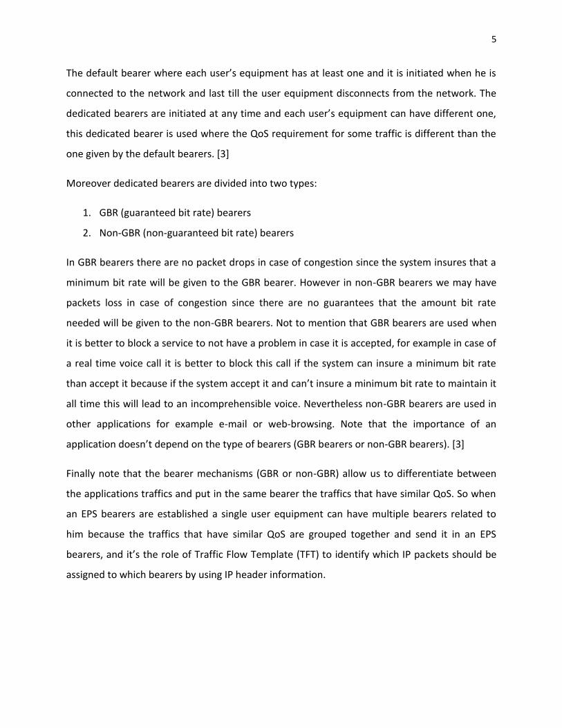
The default bearer where each user’s equipment has at least one and it is initiated when he is

connected to the network and last till the user equipment disconnects from the network. The

dedicated bearers are initiated at any time and each user’s equipment can have different one,

this dedicated bearer is used where the QoS requirement for some traffic is different than the

one given by the default bearers. [3]

Moreover dedicated bearers are divided into two types:

1. GBR (guaranteed bit rate) bearers

2. Non-GBR (non-guaranteed bit rate) bearers

In GBR bearers there are no packet drops in case of congestion since the system insures that a

minimum bit rate will be given to the GBR bearer. However in non-GBR bearers we may have

packets loss in case of congestion since there are no guarantees that the amount bit rate

needed will be given to the non-GBR bearers. Not to mention that GBR bearers are used when

it is better to block a service to not have a problem in case it is accepted, for example in case of

a real time voice call it is better to block this call if the system can insure a minimum bit rate

than accept it because if the system accept it and can’t insure a minimum bit rate to maintain it

all time this will lead to an incomprehensible voice. Nevertheless non-GBR bearers are used in

other applications for example e-mail or web-browsing. Note that the importance of an

application doesn’t depend on the type of bearers (GBR bearers or non-GBR bearers). [3]

Finally note that the bearer mechanisms (GBR or non-GBR) allow us to differentiate between

the applications traffics and put in the same bearer the traffics that have similar QoS. So when

an EPS bearers are established a single user equipment can have multiple bearers related to

him because the traffics that have similar QoS are grouped together and send it in an EPS

bearers, and it’s the role of Traffic Flow Template (TFT) to identify which IP packets should be

assigned to which bearers by using IP header information.

6

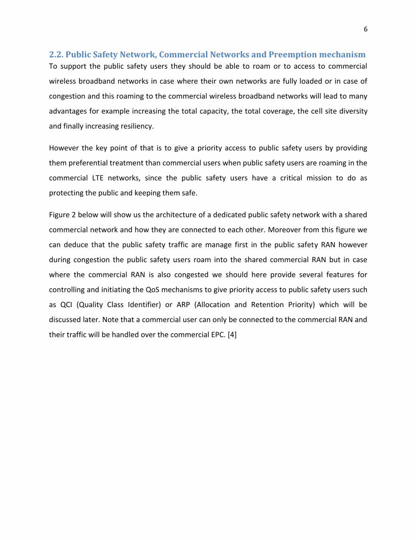
2.2. Public Safety Network, Commercial Networks and Preemption mechanism

To support the public safety users they should be able to roam or to access to commercial

wireless broadband networks in case where their own networks are fully loaded or in case of

congestion and this roaming to the commercial wireless broadband networks will lead to many

advantages for example increasing the total capacity, the total coverage, the cell site diversity

and finally increasing resiliency.

However the key point of that is to give a priority access to public safety users by providing

them preferential treatment than commercial users when public safety users are roaming in the

commercial LTE networks, since the public safety users have a critical mission to do as

protecting the public and keeping them safe.

Figure 2 below will show us the architecture of a dedicated public safety network with a shared

commercial network and how they are connected to each other. Moreover from this figure we

can deduce that the public safety traffic are manage first in the public safety RAN however

during congestion the public safety users roam into the shared commercial RAN but in case

where the commercial RAN is also congested we should here provide several features for

controlling and initiating the QoS mechanisms to give priority access to public safety users such

as QCI (Quality Class Identifier) or ARP (Allocation and Retention Priority) which will be

discussed later. Note that a commercial user can only be connected to the commercial RAN and

their traffic will be handled over the commercial EPC. [4]

7

Figure 2: Dedicated public safety network with a shared commercial network [4]

In addition when public safety users roam into a commercial network we will have four

possibilities in the shared commercial RAN shown in figure 3 below. Figure 3(a) reveal to us

where there are extra capacity not used for the both public safety users and commercial users

in the shared commercial RAN. In Figure 3(b) the commercial users is allowed to use the extra

free capacity for the public safety users since the commercial users spent all their capacity and

there are free space in the public safety users but the maximum range to which the commercial

users can enter is shown in figure 3(c) but in this case if a public safety users want to be manage

in the commercial network since his dedicated network is in congestion this public safety user

will be given a higher priority access and a commercial user will be rejected from the shared

commercial RAN and give his place to the public safety user (preemption mechanism). Finally

Figure 3(d) show the case where both the public safety and the commercial users occupy the

total capacity allocated to them. In addition in this case when a new public safety user arrives

he will be kept in the congested public safety RAN and here the priority treatment will be

applied. Moreover in case where the dedicated public safety network doesn’t suffer any more

from congestion than a chosen public safety users will be sending it back to the dedicated

public safety network to be manage their. [4]

8

Figure 3: Public safety users and commercial user in the shared commercial RAN [4]

To more clarify the preemption mechanism let us see the below figure 4 where a Matlab based

simulation is done to show the preemption mechanism when we have priority access for public

safety users in a shared commercial network. In this figure we can see that the commercial

users arrive and they use the free space dedicated for the public safety users because they

arrive faster and the public safety users are not using all their given capacity (figure 12b).

However when public safety users arrive (their dedicated public safety network is in

congestion) some commercial users are preempted and the public safety users can use their

allocated space because they are given a higher priority access (figure 4).

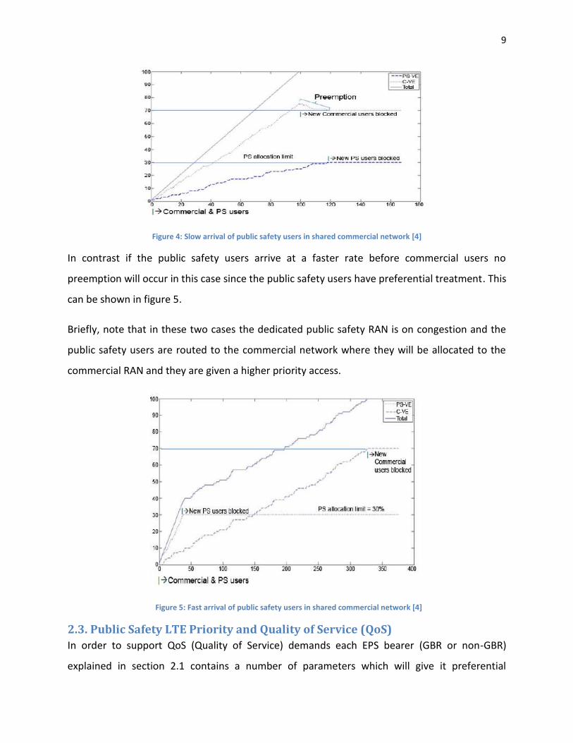
9

Figure 4: Slow arrival of public safety users in shared commercial network [4]

In contrast if the public safety users arrive at a faster rate before commercial users no

preemption will occur in this case since the public safety users have preferential treatment. This

can be shown in figure 5.

Briefly, note that in these two cases the dedicated public safety RAN is on congestion and the

public safety users are routed to the commercial network where they will be allocated to the

commercial RAN and they are given a higher priority access.

Figure 5: Fast arrival of public safety users in shared commercial network [4]

2.3. Public Safety LTE Priority and Quality of Service (QoS)

In order to support QoS (Quality of Service) demands each EPS bearer (GBR or non-GBR)

explained in section 2.1 contains a number of parameters which will give it preferential

10

treatment from other bearers. These parameters are the QoS Class Identifier (QCI) and the

Allocation and Retention Priority (ARP). Briefly to support QoS demands QCI and ARP are

needed.

2.3.1. Overview of ARP (Allocation and Retention Priority)

The ARP parameters hold three components: a single scalar and two separate flag values. The

single scalar value holds data related to the priority level of a bearer, however the two flags are

assigned to the preemption (dropping or interrupting) capability which means whether or not a

bearer is allowed to preempt other bearers which hold a lower priority level, or assigned to the

preemption vulnerability of the bearer which means whether or not a bearer is at risk to be

dropped even with a higher ARP priority level. So the ARP priority level is used to make sure

that the bearers with a higher priority level are given preferential treatment than bearers with

a lower priority level in case of congestion. Note that the ARP parameters don’t play a role in

the packet forwarding process.

Briefly ARP mechanisms allow two processes; the first process is that the lower priority level

can be preempted by a higher one and the second process where the lower priority users that

ask for request can be congested if resources are being used for higher priority users. For

example during congestion the base station (eNodeB) can discard the bearer which transport

the video component without influencing the bearer which transport the voice in a case of

video telephony application since the two components are transported into two different EPS

bearer with different ARP parameters (the voice bearer has a higher ARP priority level than the

video bearer).

Not to mention that is possible to increase the number of ARP priority levels from 16 to 64

levels by using the two spare bits in the octet which are in the present not used.

11

2.3.2. Overview of QCI (QoS Class Identifier)

Like we mention before ARP doesn’t play a role in the packet forwarding process, so the nodes

in the network use QCI to recognize how to treat the packets for each bearer. Briefly, the QCI

parameter will let the node know how to handle the packets for each bearer or to arrange the

resources between the packets following their importance, so QCI is related to the node in the

network.

QCI parameter is described by a simple scalar value. So it specifies when traffic should be sent

to or received from the mobile user equipment by considering the packet latency and the

packet loss rate in both downlink and uplink. Briefly the QCI mechanism makes sure that the

packet received at each node in the network follow to explicit QoS characteristics (packet

latency or packet delay budget and packet loss rate) and this will lead to prioritization.

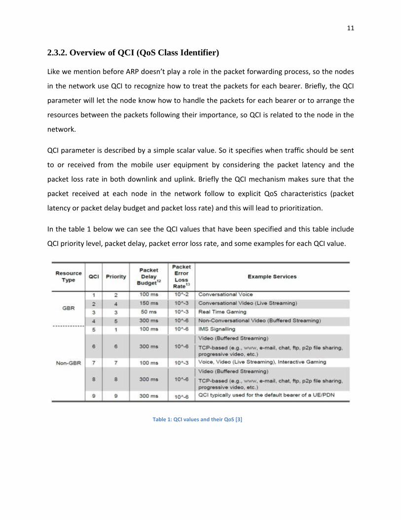
In the table 1 below we can see the QCI values that have been specified and this table include

QCI priority level, packet delay, packet error loss rate, and some examples for each QCI value.

Table 1: QCI values and their QoS [3]

12

Not to mention that nowadays only 9 out of 256 values are used for QCI so the rest value are

kept for future use which let us to say that LTE could support hundreds of QCI levels.

2.3.3. LTE Prioritization Gates

To have a better idea about the priority and QoS we can take a look at figure 6 which will

summarize the LTE prioritization gates where each user’s equipment should precede the three

gates or pass shown in the figure below before he can use wireless resources.

Figure 6: LTE prioritization gates [5]

When user equipment wants to send and receive data from an LTE network he has three gates

to use wireless resources which are given by the network. First gate as shown in figure 6 is an

access class gate, this gate decides if user equipment is authorized to interact (to be in contact)

with a specific eNodeB. The second gate is the admission (ARP) priority gate where eNodeB

decides that user equipment should be authorized to allocate system resources. Note that this

gate is the allocation and retention priority (ARP) explained before (2.3.1). The third gate is

scheduling (QCI) priority gate where the bandwidth given to specific user equipment is divided,

13

allocated and controlled or maintained the rate or speed by the system (QCI table1). Note that

this gate is the QoS Class Identifier (QCI) explained before (2.3.2).

Note that in case of congestion LTE gives a standard capability call ACB (access class barring) to

block UEs or slow down UEs from entering the system and not to mention that this happen

before admission priority gate (gate 2). So the role of ACB is to block or slow down UEs in case

of congestion and is not used in normal day to day operation so it is used for specific situations

(when a large number of responders at a given location).

Briefly, the access class value from 0 to 9 is used for commercial users so these values should

not be given to public safety users. However access class 11 is for PLMN (Public Land Mobile

Network) use, access class 12 is for security services, access class 13 is for public utilities (e.g.

Water or gas suppliers), access class 14 is used for emergency services and finally access class

15 is used for PLMN staff. In addition the access class number is registered in the users

equipment’s SIM/USIM. Note that Public Land Mobile Network (PLMN) is any wireless

communication system used by terrestrial users and it is usually connected to the fixed system

(PSTN).

2.4. Fully automated LTE system and non-fully automated LTE system

In an automated LTE system the QCI (QoS Class Identifier) and the ARP (Allocation and

Retention Priority) are given by the system following some policies and decision rules based on

the system can knows the value of a priority and can detect the value without any human

interaction, and this value are given following an agreement between the commercial

operators and public safety. However an automated LTE system in some cases can’t give the

right preferential treatment to any users so to handle these cases a non-fully automated LTE

system could be added, note that this system requires human intervention. For example an

automated LTE system can give a police officer a priority access while his making a voice call

without knowing if his pursuing a suspect or his doing a normal voice call while allowing human

intervention (non-fully automated LTE system) we can make a better decisions about

prioritization and resource allocation in the previous example this mean that we can know if

14

the police officer is doing a normal voice call or by some mechanism he can indicate if this

session is important because his pursuing a suspect. [3]

In conclusion human intervention in priority decisions can accommodate additional

functionality then an automated system provide.

2.5. Conclusion

Finally in order to supply a nationwide broadband access to public safety users during

emergencies it is essential that the public safety user can roam to a shared commercial network

and receive preferential treatment (QCI) as if they are in the home dedicated public safety

network. Not to mention that the public safety users should roam in the commercial network

without affecting the commercial users by balancing the capacity usage in the shared

commercial RAN, briefly by restricting the public safety user to a defined pre-allocated limit and

allowing the commercial user to use the free capacity if the public safety users are not using all

their allocated capacity.

15

Chapter 3

Simulation of LTE networks

3.1. Vienna LTE simulator

Vienna LTE simulators are an open-source simulation that supports the link and system level

simulations of the Universal Mobile Telecommunications System (UMTS) Long-Term Evolution

(LTE). The main role of vienna LTE simulator is to test and optimize algorithms and procedure

and this is done in both link level (LL) simulator and the system level (SL) simulator since both of

them are supported by the vienna LTE simulator. Note that the two simulators are accessible

for free for non-commercial academic use license, which helps academic research and allows a

closer teamwork between different universities and research facilities. [6]

Now let us discuss the difference between the two simulators and where each one is used and

then focusing on the system level simulator, since the LTE system level simulator the

performance of a whole network is analyzed, and the models over which this simulator is built.

3.1.1. LTE link level simulator

Link level simulations allow for the inspection of channel estimation, tracking and prediction

algorithms, synchronization algorithms, Multiple-Input Multiple-Output (MIMO) gains, Adaptive

Modulation and Coding (AMC) and feedback techniques. In addition, it can be divided into

three main blocks: Transmitter (one eNodeB), Downlink channel model, and receivers (which

are the users equipment) as we can see in figure 7.

16

Figure 7: Elements of link level simulator. [11]

Note that in the downlink channel model only the Downlink Shared Channel (DL-SCH) is transmitted where the possible modulation for this channel are 4-QAM, 16-QAM and 64-QAM.[11]

3.1.2. LTE system level simulator

System level simulations focus more on network related issues for example resource allocation

and scheduling, multi-user handling, mobility management, admission control, interference

management and network planning optimization.

Note that because of the vast amount of data processing that is needed for executing the radio

links between all terminals and base station it is impossible to perform the physical layer

simulations in this case describe before, so to perform system level simulation the physical

layer should be abstracted by reduced models without losing the main characteristics and with

high efficiency and low complication. [6]

Figure 8 below describes the schematic block diagram of the LTE system level simulator which is

divided into two parts.

First part is the link measurement model where the link quality is evaluated by using SINR

(Signal to Interface and Noise Ratio) as metric and it is required or used to give us link

adaptation and resource allocation. Note that link adaptation refers to a set of techniques

where for example modulation and coding rate parameters are changed to better match the

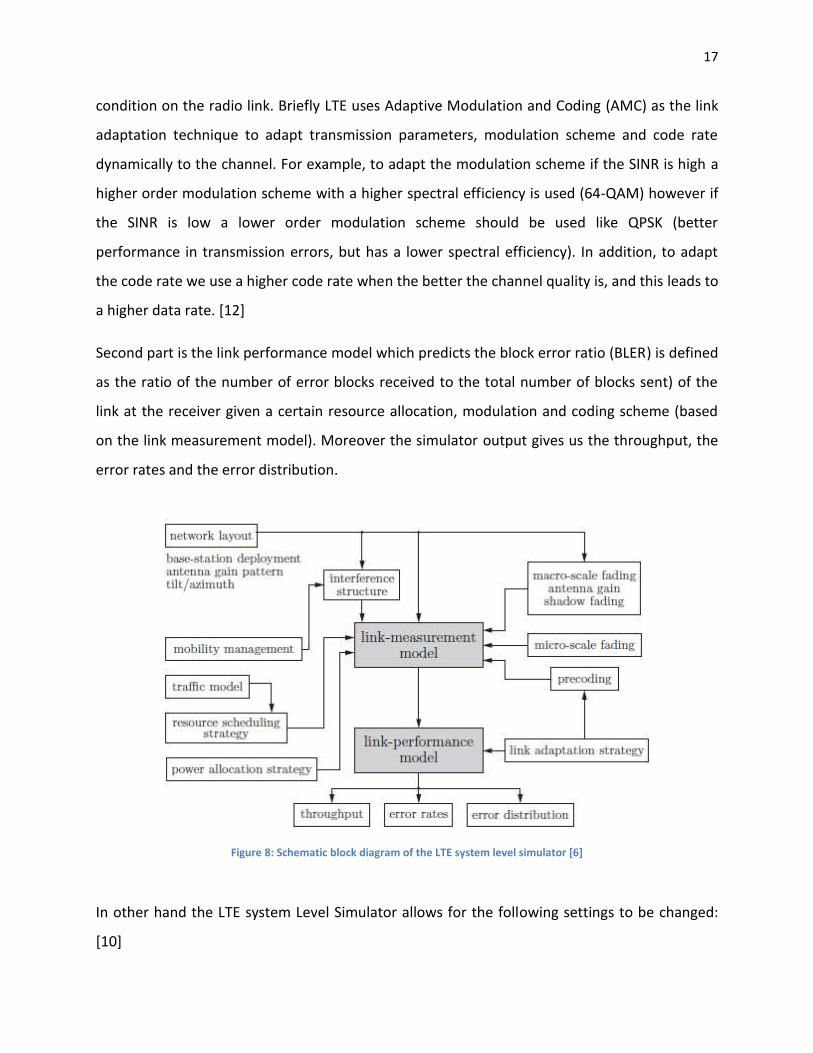
17

condition on the radio link. Briefly LTE uses Adaptive Modulation and Coding (AMC) as the link

adaptation technique to adapt transmission parameters, modulation scheme and code rate

dynamically to the channel. For example, to adapt the modulation scheme if the SINR is high a

higher order modulation scheme with a higher spectral efficiency is used (64-QAM) however if

the SINR is low a lower order modulation scheme should be used like QPSK (better

performance in transmission errors, but has a lower spectral efficiency). In addition, to adapt

the code rate we use a higher code rate when the better the channel quality is, and this leads to

a higher data rate. [12]

Second part is the link performance model which predicts the block error ratio (BLER) is defined

as the ratio of the number of error blocks received to the total number of blocks sent) of the

link at the receiver given a certain resource allocation, modulation and coding scheme (based

on the link measurement model). Moreover the simulator output gives us the throughput, the

error rates and the error distribution.

Figure 8: Schematic block diagram of the LTE system level simulator [6]

In other hand the LTE system Level Simulator allows for the following settings to be changed:

[10]

18

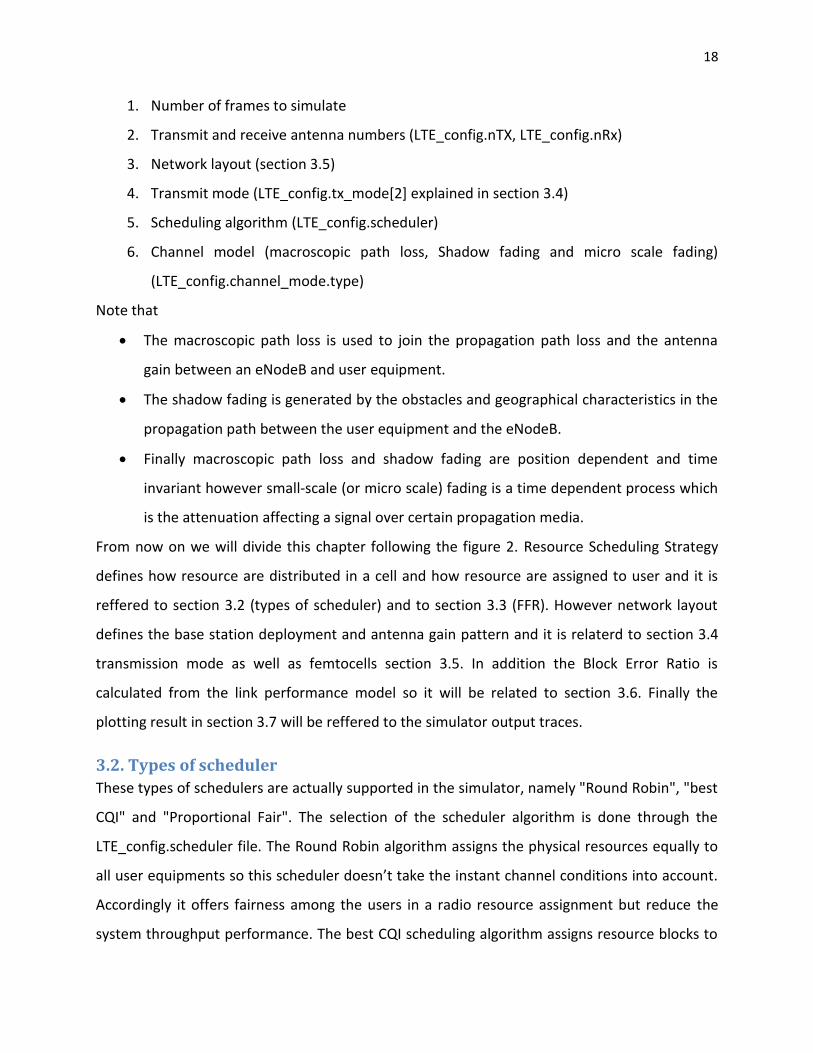
1. Number of frames to simulate

2. Transmit and receive antenna numbers (LTE_config.nTX, LTE_config.nRx)

3. Network layout (section 3.5)

4. Transmit mode (LTE_config.tx_mode[2] explained in section 3.4)

5. Scheduling algorithm (LTE_config.scheduler)

6. Channel model (macroscopic path loss, Shadow fading and micro scale fading)

(LTE_config.channel_mode.type)

Note that

The macroscopic path loss is used to join the propagation path loss and the antenna

gain between an eNodeB and user equipment.

The shadow fading is generated by the obstacles and geographical characteristics in the

propagation path between the user equipment and the eNodeB.

Finally macroscopic path loss and shadow fading are position dependent and time

invariant however small-scale (or micro scale) fading is a time dependent process which

is the attenuation affecting a signal over certain propagation media.

From now on we will divide this chapter following the figure 2. Resource Scheduling Strategy

defines how resource are distributed in a cell and how resource are assigned to user and it is

reffered to section 3.2 (types of scheduler) and to section 3.3 (FFR). However network layout

defines the base station deployment and antenna gain pattern and it is relaterd to section 3.4

transmission mode as well as femtocells section 3.5. In addition the Block Error Ratio is

calculated from the link performance model so it will be related to section 3.6. Finally the

plotting result in section 3.7 will be reffered to the simulator output traces.

3.2. Types of scheduler

These types of schedulers are actually supported in the simulator, namely "Round Robin", "best

CQI" and "Proportional Fair". The selection of the scheduler algorithm is done through the

LTE_config.scheduler file. The Round Robin algorithm assigns the physical resources equally to

all user equipments so this scheduler doesn’t take the instant channel conditions into account.

Accordingly it offers fairness among the users in a radio resource assignment but reduce the

system throughput performance. The best CQI scheduling algorithm assigns resource blocks to

19

the user with the best radio link condition. Note that a higher CQI value means better channel

condition and CQI refer to channel quality indicator which is a summary of the channel

condition under the current transmission. Moreover, the base station in the downlink transmits

reference signal to user equipment and these reference signals are used by user equipments for

the measurement of the CQI and then user equipments send channel quality indicator (CQI) to

the base station in order to perform scheduling. It is important to mention that in this

scheduling terminal located far from the base station are rare to be scheduled. Finally the

proportional fair scheduler operates between the best CQI scheduling and round robin

scheduling. Proportional fair exploits user diversity by selecting the user with the best condition

to transmit during different time slots so this scheduler show an acceptable throughput level

while providing some fairness between users. In this figure 9 below we can see the scheduler

comparison in terms of mean, edge and peak user equipment throughput the fairness is shown

in the legend.

Figure 9: Scheduler comparison [7]

Note that the mean throughput refers to cell average, edge throughput refers to users located

at the cell edge which indicate the cell borders and peak throughput stands for the maximum

20

achievable throughput in optimal condition. Like we see in the figure best CQI scheduler works

on the mean throughput and has achieved its higher throughput at the peak throughput

however on the edge throughput this scheduler turn to be zero because terminals are located

far from the base station and they are unlikely to be scheduled like we said before.

Furthermore since round robin ignores the channel quality information it usually results in

lower user and overall network throughput levels. We can notice that best CQI scheduling can

increase the cell capacity at the price of the fairness between user equipments. Finally by using

a proportional fair scheduler we can notice that we are increasing the system throughput

compared to a round robin scheduler by serving user in a fair manner.

3.3 Fractional Frequency Reuse (FFR)

It is important to mention that FFR is implemented in the LTE system level simulator as a new

kind of scheduler called FFR scheduler and allows to identify a scheduler for the FR (Full Reuse)

and PR (Partial reuse) parts independently. For example the activation of the FFR schedular is

done through the LTE_config.FFR_active and know we should identify a scheduler for the FR

and PR parts as e.g. roud robin or proportional fair scheduler, and this is done through the

LTE_config.scheduler_params.FR_scheduler.scheduler [7] for the FR parts and should be equal

to the type of the scheduler we need to assign to it as well as for the PR parts it is done through

the LTE_config.scheduler_params.FR_scheduler.scheduler [7] .

Not to mention that FFR refers to fractional frequency reuse where different parts of available

spectrum are allocated to different users depending on their location in the cell. To clarify more

we can see figure 10 where the users closer to cell center are scheduled in frequency band with

frequency reuse one however users close to cell borders (edge) are scheduled in other parts of

the available spectrum with partial reuse such that the signals are orthogonal to the neighbor

users. Briefly this technique consist of splitting the bandwidth into two parts: FR (full reuse) and

PR (partial reuse) for the cell edge users and is used to reduce ICI (inter cell interference)

caused by OFDMA system.

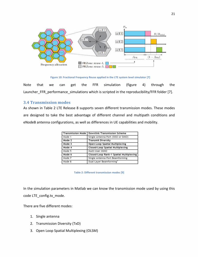
21

Figure 10: Fractional Frequency Reuse applied in the LTE system level simulator [7]

Note that we can get the FFR simulation (figure 4) through the

Launcher_FFR_performance_simulations which is scripted in the reproducibility/FFR folder [7].

3.4 Transmission modes

As shown in Table 2 LTE Release 8 supports seven different transmission modes. These modes

are designed to take the best advantage of different channel and multipath conditions and

eNodeB antenna configurations, as well as differences in UE capabilities and mobility.

Table 2: Different transmission modes [9]

In the simulation parameters in Matlab we can know the transmission mode used by using this

code LTE_config.tx_mode.

There are five different modes:

1. Single antenna

2. Transmission Diversity (TxD)

3. Open Loop Spatial Multiplexing (OLSM)

22

4. Closed Loop Spatial Multiplexing (CLSM)

5. Multiuser MIMO (this one is not yet implemented)

Where TxD is used to reduce the effects of fading, which is the attenuation affecting a signal

over certain propagation media, by transmitting the same information from two different

antennas. However spatial multiplexing is a transmission technique in MIMO (multiple inputs

and multiple outputs where we use multiple antennas at both the transmitter and receiver side

to send multiple parallel signals and by doing that we are improving communication

performance) wireless communication used in LTE downlink which transmit independent

encoded data from each of the multiple transmit antennas. Like we saw before that Spatial

Multiplexing is divided into two modes the first one is the Open Loop Spatial Multiplexing

(OLSM) where user equipments reports the rank indicator (RI) and the channel quality indicator

(CQI). The second Closed Loop Spatial Multiplexing where the user equipments reports the RI,

CQI and the precoding matrix indicator (PMI).

Note that the CQI is an indicator which let us to know how good or bad the communication

channel quality is and its depend at which value the user equipments reports the network will

transmit data with large or small transport blocks. Briefly CQI is a summary of the channel

condition under the current transmission. RI is the best number of streams a user would like to

receive for example RI equal to one UE can’t separate two transport blocks so it use

transmission diversity, for RI equal to two user equipment is able to separate two transport

blocks so eNodeB can use MIMO transmission techniques and finally PMI is used only in CLSM

where user equipments indicates to eNodeB how to map the data on the two antennas to

optimize reception with selected codebook index. Briefly PMI determines the best precoding

matrix for the current channel conditions. Finally it’s important to mention that spatial

multiplexing requires multipath to work and provide extra gain as compared to TxD.

The figure 11 below show the difference in throughput respect to signal to noise ratio (SNR) in

two different modes which are SISO where we have one transmitting and one receiving

antenna and TxD where we transmit information from two different antennas. We notice that

by using TxD transmission mode for system and link level the throughput will be higher than

23

using SISO transmission mode till SNR equal to 26 dB because when SNR will be equal to 20 dB

the throughput (using TxD transmission mode) will be stable and like that by using SISO

transmission mode it will be better than TxD above 26 dB.

Note that SNR stands for signal to noise ratio which is a measure that compares the level of a

desired signal to the level of noise. Moreover a ratio higher than 0 dB indicates more signal

than noise.

Figure 11: SISO and TxD transmission mode [7]

Figure 12 below show the difference by using CLSM 2x2, CLSM 4x2 and CLSM 4x4. By using

CLSM 2x2 we double the capacity and throughput however by using CLSM 4x4 we quadruple

the capacity and throughput. In addition NxN stand for the number of antennas used to

transmit signals from the base station and the number of antennas to receive signals from

mobile terminal or user equipments for example 2x2 configuration is two antennas to transmit

signal from the base station and two other antennas to receive signals. We can deduce from

the figure that by using CLSM 4x4 we have more throughput than using CLSM 2x2 because we

double the capacity and throughput.

24

Figure 12: Throughput comparison for CLSM NxN [7]

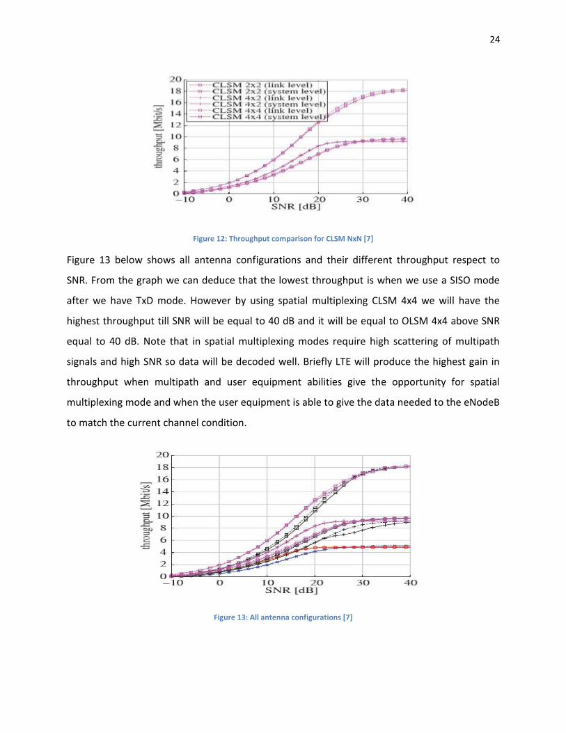
Figure 13 below shows all antenna configurations and their different throughput respect to

SNR. From the graph we can deduce that the lowest throughput is when we use a SISO mode

after we have TxD mode. However by using spatial multiplexing CLSM 4x4 we will have the

highest throughput till SNR will be equal to 40 dB and it will be equal to OLSM 4x4 above SNR

equal to 40 dB. Note that in spatial multiplexing modes require high scattering of multipath

signals and high SNR so data will be decoded well. Briefly LTE will produce the highest gain in

throughput when multipath and user equipment abilities give the opportunity for spatial

multiplexing mode and when the user equipment is able to give the data needed to the eNodeB

to match the current channel condition.

Figure 13: All antenna configurations [7]

25

3.5. Femtocells

Finally let us talk about femtocells since the LTE system level simulator permits for an additional

layer of a node to be added over the standard eNodeB grid. So in Matlab by using this function

LTE_config.femtocells function we are adding a layer called femtocells or small cells. In addition

by adding this layer we can specify the spatial distribution of femtocells for example it can be

homogeneously spread or we can know what is the transmit power of each of the femtocells in

watts and which path loss model are used.

Not to mention that due to the increasing indoor phone calls and data transfers and because of

the lack macrocell coverage so the femtocells will be a good solution in the near future. Where

femtocell is a wireless access point act as a repeater so it increases cellular reception for

example of data inside a home or office building. In addition this device communicates with the

mobile phone and changes voice calls into voice over IP packets which will be transmitted to

the operator’s servers. In contrast macrocell provide radio coverage served by a high tower

(base station) which should be installed on a ground or on a rooftop so it will be installed with a

clear view. [9]

3.6. SNR to CQI mapping

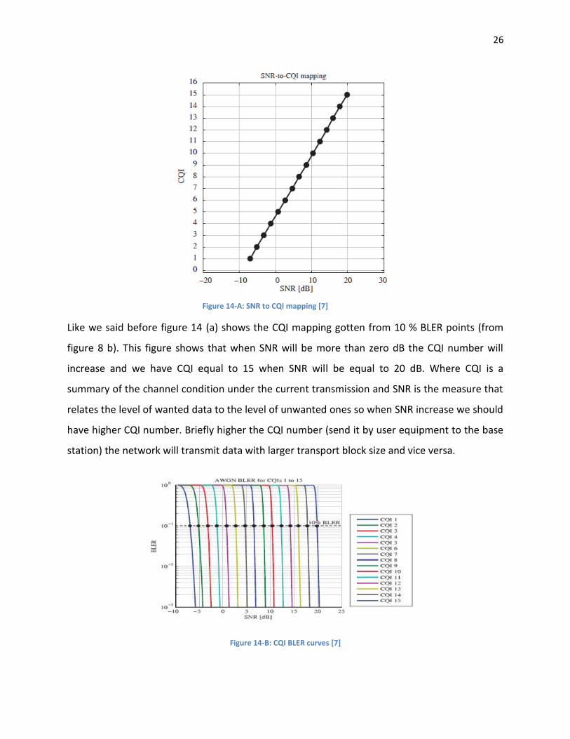
BLER which stand for Block Error Ratio curve data files can be provided to the simulator from

LTE link-level simulator.mat results file and this file contain two vectors (SNR value and BLER

value) of equal length. Moreover the CQI table are used to generate the SNR to CQI mapping

which is shown in figure 14 (a & b). The 15 CQI BLER are shown in figure 14 (b) and from their

10% BLER points we can get the CQI mapping (figure 14 a). [7]

26

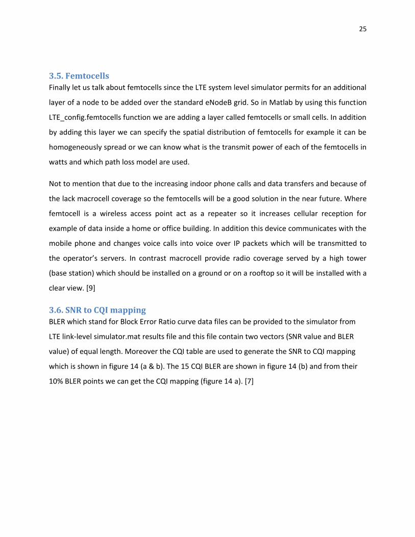
Like we said before figure 14 (a) shows the CQI mapping gotten from 10 % BLER points (from

figure 8 b). This figure shows that when SNR will be more than zero dB the CQI number will

increase and we have CQI equal to 15 when SNR will be equal to 20 dB. Where CQI is a

summary of the channel condition under the current transmission and SNR is the measure that

relates the level of wanted data to the level of unwanted ones so when SNR increase we should

have higher CQI number. Briefly higher the CQI number (send it by user equipment to the base

station) the network will transmit data with larger transport block size and vice versa.

Figure 14-B: CQI BLER curves [7]

Figure 14-A: SNR to CQI mapping [7]

27

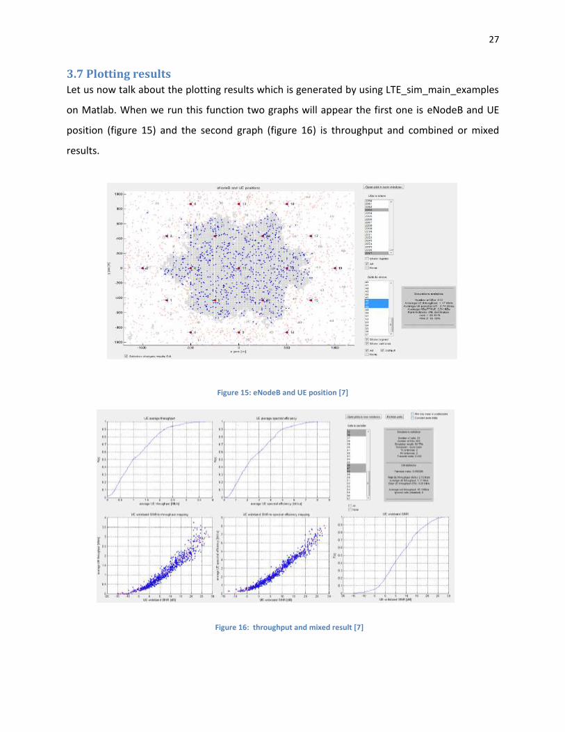
3.7 Plotting results

Let us now talk about the plotting results which is generated by using LTE_sim_main_examples

on Matlab. When we run this function two graphs will appear the first one is eNodeB and UE

position (figure 15) and the second graph (figure 16) is throughput and combined or mixed

results.

Figure 15: eNodeB and UE position [7]

Figure 16: throughput and mixed result [7]

28

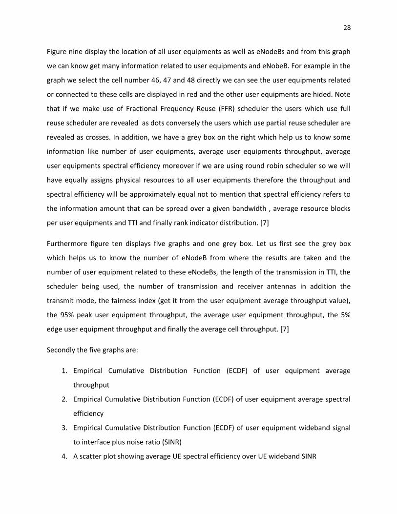
Figure nine display the location of all user equipments as well as eNodeBs and from this graph

we can know get many information related to user equipments and eNobeB. For example in the

graph we select the cell number 46, 47 and 48 directly we can see the user equipments related

or connected to these cells are displayed in red and the other user equipments are hided. Note

that if we make use of Fractional Frequency Reuse (FFR) scheduler the users which use full

reuse scheduler are revealed as dots conversely the users which use partial reuse scheduler are

revealed as crosses. In addition, we have a grey box on the right which help us to know some

information like number of user equipments, average user equipments throughput, average

user equipments spectral efficiency moreover if we are using round robin scheduler so we will

have equally assigns physical resources to all user equipments therefore the throughput and

spectral efficiency will be approximately equal not to mention that spectral efficiency refers to

the information amount that can be spread over a given bandwidth , average resource blocks

per user equipments and TTI and finally rank indicator distribution. [7]

Furthermore figure ten displays five graphs and one grey box. Let us first see the grey box

which helps us to know the number of eNodeB from where the results are taken and the

number of user equipment related to these eNodeBs, the length of the transmission in TTI, the

scheduler being used, the number of transmission and receiver antennas in addition the

transmit mode, the fairness index (get it from the user equipment average throughput value),

the 95% peak user equipment throughput, the average user equipment throughput, the 5%

edge user equipment throughput and finally the average cell throughput. [7]

Secondly the five graphs are:

1. Empirical Cumulative Distribution Function (ECDF) of user equipment average

throughput

2. Empirical Cumulative Distribution Function (ECDF) of user equipment average spectral

efficiency

3. Empirical Cumulative Distribution Function (ECDF) of user equipment wideband signal

to interface plus noise ratio (SINR)

4. A scatter plot showing average UE spectral efficiency over UE wideband SINR

29

5. A scatter plot showing the wideband SINR over the spectral efficiency.

Not to mention that SINR is a measure of the signal quality which determine the relation

between radio frequency conditions and the throughput, UE use SINR to compute the CQI and

then report this value to the network.

3.8. Conclusion

In conclusion in this part we highlighted on the models over which the simulator is built and we

evaluate the performance of LTE using system lever simulator, For example by describing the

core part of the system level simulator and the comparison of the scheduler types the user

throughput, the CQI, SNR and many others. In my opinion LTE system level simulator will play a

good role in making mobile communication better and better through analyzing the output

result and finding solutions for the problems which occur and since it is a non-commercial

academic use where every person interested in this field can develop some algorithm to fix the

problem.

30

Chapter 4

Performance assessment of prioritization capabilities

4.1. Prioritization mechanism

The prioritization mechanism is designed as an extension of the PF scheduling. In particular, the

PF algorithm has been modified to account for the priority level embedded in the QCI value.

The resulting scheduler is named QCI-aware PF scheduler. Next subsection describes both

algorithms.

4.1.1 Proportional Fair (PF) scheduling:

The proportional Fair (PF) scheduling algorithm is based on maximizing the scheduling metric.

In more details for any resource block in any TTI this scheduler schedules only the user with the

maximum performance metric (max PM).

In mathematics it can be shown as follows:

(Eq.1)

Where:

K is the selected user in the ith CC at the jth RB in time τ

R is the estimated throughput of the user k in the ith CC at the jth RB in time τ which will

be in our case later the instantaneous throughput (Rinst).

r is the average throughput in the past of the user k in the ith CC in the time τ which will

be in our case later the accumulative throughput (Raccum).

Note that τ refers to TTI, j refers to the number of RB and finally CC refers to Component

Carrier.

In the PF scheduler the metric used by the programmer is calculated as follow:

31

Metric= (Cx12x7)/Ralphatemp (in log scale) (Eq.2)

Where alphatemp=1; R represent the accumulated throughput in bit/s; however C represent

the BICS (Bit Interleaved Coded Modulation) efficiency which is here in bits/channel use,

because of that we multiply it by 12x7 ( 12 represent the subcarrier and 7 the symbols) to get

the instantaneous throughput for a specific user. Not to mention that the “obj.d” and obj.k”

used to calculate C (BICS efficiency) in “LTEScheduler” are the coefficients from the linear fit in

order to avoid nonlinearity and this linear fit has to be applied depend on the actual value of

CQI for each user[13].

In addition, in the simulator we have a total number of users divided into 57 cells where each

cell contains a fix number of users. Moreover, the simulator contains 19 eNodeBs and each

three cells are attached to one eNodeB.

From that we can understand how the simulator pass the users in each TTI, for that lets focus in

the first TTI (TTI=1) since for the others TTIs in the simulator repeat the same method for the

same users. So for the first TTI we have 57 cells, in the first cell we have the number of users

that we fixed and for each one of these users have an average throughput (Raccum) and an

instantaneous throughput (Rinst), moreover these numbers of users have 100 resource blocks

available since the bandwidth is equal to 20 MHZ in each TTI.

After finding the maximum value in the metric calculated as showed before, the users that

should be allocated resource block to them are putted in an array called RBs, which include

zero and one where one represents the user that should be allocated a resource block and

these users are putted in a list called UE_id_list to allocate to them resource block. Note that to

avoid allocating many users to one resource block because maybe they have the same value

that has been calculated following equation 2, the programmer use a function ind = randi

(length(RB_idx)) so by doing that the programmer is allocating a resource block for only one

user.

32

4.2 Validation of the simulator

To validate the simulator we will see first the relation between the instantaneous throughput

and the accumulated throughput and how is computed in section 4.1.2.1, and then we will see

how the dynamic of the simulator works in section 4.1.2.2.

4.2.1 Validation of the instantaneous throughput and the accumulated

throughput and see how there are connected.

First before starting with the validation of the instantaneous and the accumulated throughput

let us see now under which scenario the PF scheduler has been addressed:

Antenna configuration:

Number of Tx Antenna: 2

Number of Rx Antenna: 2

Transmission mode = Closed Loop Spatial Multiplexing (CLSM)

Number of eNodeBs: 19

Total number of users: 570 users only 210 users are active since the simulator computes

only users from cells numbers: 1, 13, 14, 15, 16, 17, 18, 19, 20, 21, 28, 29, 30, 31, 32, 33,

34, 35, 36, 46 and 48. Note that here in each cell we have ten users.

Spatial distribution of terminals: Each three cells are connected to one eNodeB

Traffic model: Full Buffer

Bandwidth= 20 MHz (Number of RBs= 100 each TTI)

Simulation time TSIM (TTI) = 10, 20, 30, 50 and 500

Average window size of 20 TTI for the accumulative throughput

Secondly, to simplify our calculation we run the simulator at TTI=10 for the first time where we

have cell number one active containing ten users and connected to eNodeB number one. In this

case figure 17 displays the accumulated throughput (Raccum) and the instantaneous

throughput (Rinst) for user number one in the cell number one.

33

Figure 17: Raccum and Rinst for user number one in cell number one at TTI=10

Here the X axis represents the number of TTI and Y axis represents the throughput in bits/s

conversely the blue line represents the Rinst (instantaneous throughput) of the user number

one in cell number one at each TTI and the red line represent the Raccum (accumulated

throughput) of the user number one in cell number one at each TTI.

In addition Rinst and Raccum here are related following this function:

Raccum(n)= (1 – alpha) . Raccum (n-1) + (alpha). Rinst

Where Raccum(n) represents the accumulative throughput at a specific TTI , Raccum (n-1)

represents the previous accumulative throughput at TTI-1, finally Rinst represents the

instantaneous throughput of this user at a specific TTI.

Furthermore it is important to mention that alpha from TTI = 1 till TTI = 10 is computed as 1/TTI

number, for example in TTI equal to two alpha is equal to 1/2, for TTI equal to five alpha is

equal to 1/5. However for TTI above ten always alpha will be equal to 1/10, for example for TTI

equal to sixteen alpha will be equal to 0.1.

Now let’s take some examples to know how we can compute Raccum is calculated:

For the TTI= 1, alpha is equal 1 so Raccum = (alpha)Rinst= Rinst= 208000 bits/s

1 2 3 4 5 6 7 8 9 100

0.5

1

1.5

2

2.5

3

3.5

4x 10

6

TTI

thro

ughput

of

user

num

ber

1 in c

ell

1 (

bits/s

ec)

Rinst

Raccum

34

For TTI=2, alpha is equal 0.5 so Raccum= (0.5) Raccum (of TTI=1) + (0.5) Rinst == (0.5) (208000)

+ (0.5) (208000) = 208000 bit/s

For TTI= 5, alpha is equal 0.2 so Raccum= (1-0.2) Raccum (of TTI=4) + (0.2) Rinst == (0.8)

(908000) + (0.2) (3512000) = 1428800 bit/s

Moreover if we run the simulator at TTI=20 (Figure 18) to check if the alpha is stable now, and

equal to 0.1 above TTI=10. So finally by calculating the Raccum at a different TTI above ten we

found that alpha is equal to 0.1.

Figure 18: Raccum and Rinst for user number one in cell number one at TTI=20

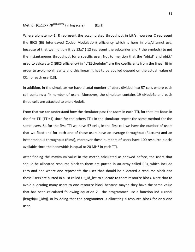
For example in the Figure 18, for TTI=15, alpha is equal 0.1 so Raccum(of this user at TTI=15)=

(1-0.1) Raccum (of TTI=14) + (0.1) Rinst == (0.9) (2682000) + (0.1) (824000) = 2496000 bit/s and

by comparing this result to the graph we will find that it’s the case. Note that these values that

we got are showed in figure 18 (a), figure 18(b) and figure 18(b).

0 2 4 6 8 10 12 14 16 18 200

0.5

1

1.5

2

2.5x 10

7

TTI

thro

ughput

of

user

num

ber

1 in c

ell

1 (

bits/s

ec)

Raccum

Rinst

35

Figure 18 a : Value of Rinst at TTI equal to 15

Figure 18 b: Value of Raccum at TTI equal to 14

10 11 12 13 14 15 16 17 18 19 200

2

4

6

8

10

12

x 106

X: 15

Y: 8.24e+05

TTI

thro

ughput

of

user

num

ber

1 in c

ell

1 (

bits/s

ec)

Raccum

Rinst

10 11 12 13 14 15 16 17 18 190

2

4

6

8

10

12

x 106

X: 14

Y: 2.682e+06

TTI

thro

ughput

of

user

num

ber

1 in c

ell

1 (

bits/s

ec)

Raccum

Rinst

36

Figure 18 c : Value of Raccum at TTI equal to 15

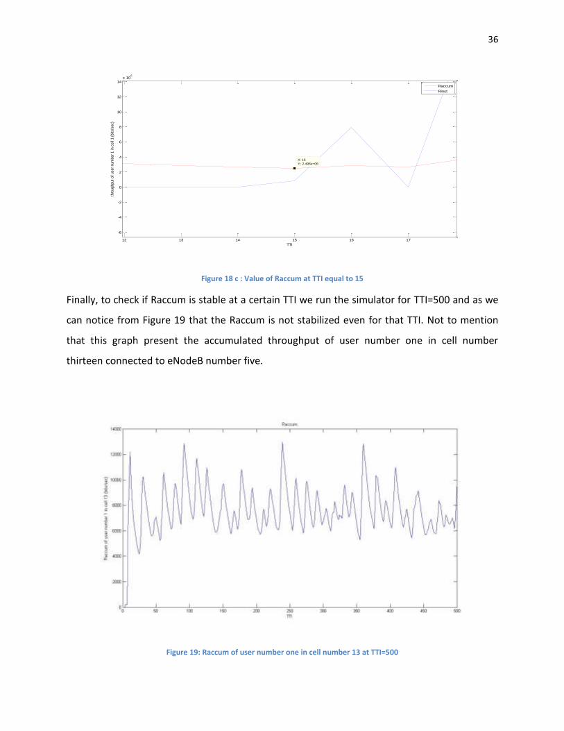
Finally, to check if Raccum is stable at a certain TTI we run the simulator for TTI=500 and as we

can notice from Figure 19 that the Raccum is not stabilized even for that TTI. Not to mention

that this graph present the accumulated throughput of user number one in cell number

thirteen connected to eNodeB number five.

Figure 19: Raccum of user number one in cell number 13 at TTI=500

12 13 14 15 16 17

-6

-4

-2

0

2

4

6

8

10

12

14x 10

6

X: 15

Y: 2.496e+06

TTI

thro

ughput

of

use

r num

ber

1 in

cell

1 (

bits

/sec)

Raccum

Rinst

37

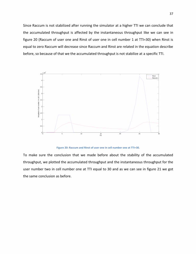
Since Raccum is not stabilized after running the simulator at a higher TTI we can conclude that

the accumulated throughput is affected by the instantaneous throughput like we can see in

figure 20 (Raccum of user one and Rinst of user one in cell number 1 at TTI=30) when Rinst is

equal to zero Raccum will decrease since Raccum and Rinst are related in the equation describe

before, so because of that we the accumulated throughput is not stabilize at a specific TTI.

Figure 20: Raccum and Rinst of user one in cell number one at TTI=30.

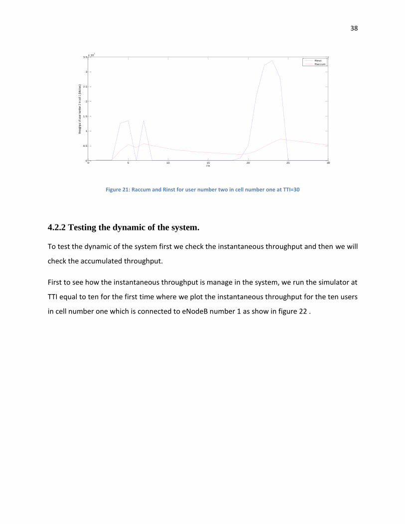
To make sure the conclusion that we made before about the stability of the accumulated

throughput, we plotted the accumulated throughput and the instantaneous throughput for the

user number two in cell number one at TTI equal to 30 and as we can see in figure 21 we got

the same conclusion as before.

0 5 10 15 20 25 300

0.5

1

1.5

2

2.5

3

3.5

4

4.5x 10

7

TTI

thro

ughput

of

user

num

ber

1 in c

ell

1 (

bits/s

ec)

Rinst

Raccum

38

Figure 21: Raccum and Rinst for user number two in cell number one at TTI=30

4.2.2 Testing the dynamic of the system.

To test the dynamic of the system first we check the instantaneous throughput and then we will

check the accumulated throughput.

First to see how the instantaneous throughput is manage in the system, we run the simulator at

TTI equal to ten for the first time where we plot the instantaneous throughput for the ten users

in cell number one which is connected to eNodeB number 1 as show in figure 22 .

0 5 10 15 20 25 300

0.5

1

1.5

2

2.5

3

3.5x 10

7

TTI

thro

ughp

ut o

f us

er n

umbe

r 2

in c

ell 1

(bi

ts/s

ec)

Rinst

Raccum

39

Figure 22: Rinst for the ten users in cell number one at TTI=10

So like we can notice from TTI equal to zero till TTI equal to ten the system is in a warning

period however like we will see later in Figure 24 that the simulator above TTTI equal to ten will

be in a steady state.


Now the Rinst for the ten users in cell number one at TTI equal to 30 is showed in figure 23.

First as we can see in the legend each line color presents the Rinst for a specific user for

1 2 3 4 5 6 7 8 9 100

1

2

3

4

5

6

7

8x 10

7

TTI

thro

ughput

in b

its/s

ec

Sum of Rinst for the 10 users in cell 1

Rinst for user 1 in cell 1










0 5 10 15 20 25 300

1

2

3

4

5

6

7

8x 10

7

TTI

thro

ughput

in b

its/s

ec












40

example the red line presents the instantaneous throughput (Rinst) for user number 5,

however the blue dashed line presents the summation of Rinst in each TTI.

As we can realize from figure 23 for TTI equal to 0 till 10 we can’t have a clear view about how

the system distribute the capacity for the 10 users, so we are sure now that the system below

TTI equal to ten the system is in a warning period. However for TTI equal to 10 and above we

can see clearly now how Rinst is distributed among the 10 users. It is between 5 and 7 TTI (5 or

7 ms) a specific user has a higher Rinst than the others users. So finally we can say that the

dynamic of this process work as following, between 5 and 7 TTI a specific user will have a higher

Rinst than the other users, then while the Rinst of this specific user will start to decrease, at this

moment Rinst of another user will start to increase till he gets a higher Rinst between all the

other users. For example as we can see in the graph user number one (present it in blue line)

when his Rinst start to increase the Rinst of user number two (present it in green line) start to

decrease. Not to mention that at 25 TTI user number one will have a higher Rinst then the

others users.

Note that when the summation of Rinst for the 10 users decrease all the Rinst at this specific

TTI will be small and this case that we are talking about is present it in TTI equal to 8 till 11.

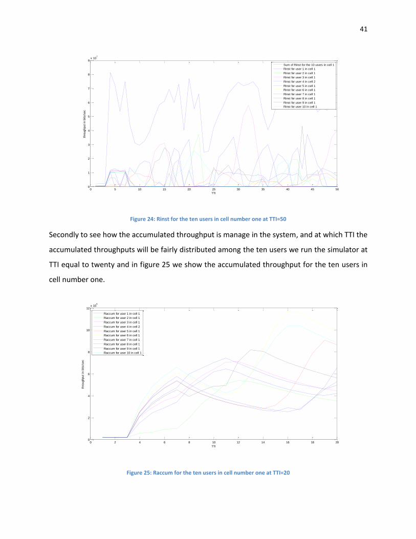
To make sure about the conclusion that we just made it about how the dynamic of this process

work, we run the simulator at TTI equal to fifty as show figure 24 and as we can see in the

following figure we got the same conclusion that we got it before.

41


Secondly to see how the accumulated throughput is manage in the system, and at which TTI the

accumulated throughputs will be fairly distributed among the ten users we run the simulator at

TTI equal to twenty and in figure 25 we show the accumulated throughput for the ten users in

cell number one.

Figure 25: Raccum for the ten users in cell number one at TTI=20

0 5 10 15 20 25 30 35 40 45 500

1

2

3

4

5

6

7

8

9x 10

7

TTI

thro

ughput

in b

its/s

ec












0 2 4 6 8 10 12 14 16 18 200

2

4

6

8

10

12x 10

6

TTI

thro

ughput

in b

its/s

ec

Raccum for user 1 in cell 1










42

Like we can see from figure 25 the accumulated throughput at TTI equal to twenty is not yet

fairly distributed among the ten users. However if we run the simulator at TTI equal to fifty as

we can get from Figure 26 the accumulated throughputs at TTI equal to fifty the are more fairly

distributed between the ten users, so we decided to fix TTI at 50.

Figure 26: Raccum for the ten users in cell number one at TTI=50

4.3 QCI-aware Proportional Fair (PF) scheduling.

So far we explained how the proportional fair scheduler is working without adding priority

access to it. By adding the QoS Class Identifier (QCI) to each user we need now to take into

consideration the QCI number of each user.

So the new mechanism that we added is to introduce in the metric calculated in the PF

scheduler (Eq.2) an alpha for the users so like that we can differentiate now between users

following their QCI numbers, so the new formula will be as following:

Metric= (C x12x7xalpha)/Ralphatemp (Eq.3)

0 5 10 15 20 25 30 35 40 45 500

1

2

3

4

5

6

7

8

9

10x 10

6

TTI

thro

ughput

in b

its/s

ec











43

4.3.1 Simulation results:

The performance analysis of QCI-aware PF scheduler has been addressed under the following

scenario settings:

Antenna configuration:

Number of Tx Antenna: 2

Number of Rx Antenna: 2

Transmission mode = Closed Loop Spatial Multiplexing (CLSM)

Number of eNodeBs: 19

Total number of users: First if we have 10 users per cell we will have 570 users in total,

only 210 users are active since the simulator computes only users from cells numbers: 1,

13, 14, 15, 16, 17, 18, 19, 20, 21, 28, 29, 30, 31, 32, 33, 34, 35, 36, 46 and 48. However if

we modify the simulator to have sixteen users per cell the total number of users will be

912 users. Finally if we decide to have twenty users per cell the total number of users

will be 1140 users. Not to mention that in the simulation results I will focus only in the

users in cell number one.

Spatial distribution of terminals: Each three cells are connected to one eNodeB.

QCI configuration: two QCI values (Being the users with QCI1 higher priority), however

we will focus in the following case where the percentage of terminals with QCI1 and QCI2

Beta=50% so like that half the users will have QCI1 and the other half users will have a

QCI2.

Traffic model: Full Buffer.

Bandwidth= 20 MHz (Number of RBs= 100 each TTI)

Simulation time TSIM = 50 TTI

Average window size of 20 TTI for the accumulative throughput

From now on we will focus our study on the accumulated throughput to understand what will

happen with the accumulated throughputs of the users when these users will receive different

QCI numbers.

44

Now to see which alpha numbers (introduced in Eq.3) we should pick for the users that have

QCI1 and for the users that have QCI2, first we gave to user number one in cell number one an

alpha equal to one and for the others nine users (in the same cell) we gave them an alpha equal

to 0.5, so like that I am giving a priority access to user number one over the nine users that we

have in cell number one. So we are assuming here that user number one has a QCI1, however

user two till ten have QCI2.

Figure 27 illustrates the accumulative throughput for each user in cell number one and as we

can deduce the accumulated throughput of user number one in cell number one has the

highest value from the other nine users but the gap between them is very high at TTI equal to

fifty. This gap between user number one and the other nine users will be equal to times nine.

Figure 27: Raccum for the ten users in cell number one with alpha equal to 1 and 0.5

Because the gap that we got in this scenario at these two values of alpha is very high, and if we

run the simulator with an alpha equal to one and 0.8, first user in cell number one has an alpha

equal to one and for the others nine users have an alpha equal to 0.8, the gap between the

accumulated throughput at TTI equal to fifty between user number one and the others nine

users will be less than before and more reasonable as we can see in Figure 28. This gap will be

0 5 10 15 20 25 30 35 40 45 500

0.5

1

1.5

2

2.5

3

3.5

4

4.5

5x 10

7

TTI

thro

ughput

in b

its/s

ec











45

equal to times three. Not that like we said before at TTI below ten the system is in a warning

period so at TTI above ten the system will be in a steady state.

Figure 28: Raccum for the ten users in cell number one with alpha equal to 1 and 0.8

However if we have twenty users per cell and if we took alpha equal to 0.8 the accumulated

throughputs of the users at TTI equal to 50 will overlap for the both kind of users (users that

have QCI1 and QCI2) as showed in figure 29. Note that the blue line presents the users that have

priority (QCI1), however the red line present the users with lowest priority (QCI2).

Figure 29: Raccum for the 20 users in cell number one with alpha equal to 1 and 0.8

0 5 10 15 20 25 30 35 40 45 500

0.5

1

1.5

2

2.5x 10

7

X: 50

Y: 1.844e+07

TTI

thro

ughp

ut in

bits

/sec











0 5 10 15 20 25 30 35 40 45 500

1

2

3

4

5

6

7

8x 10

6

TTI

thro

ughput

in b

its/s

ec

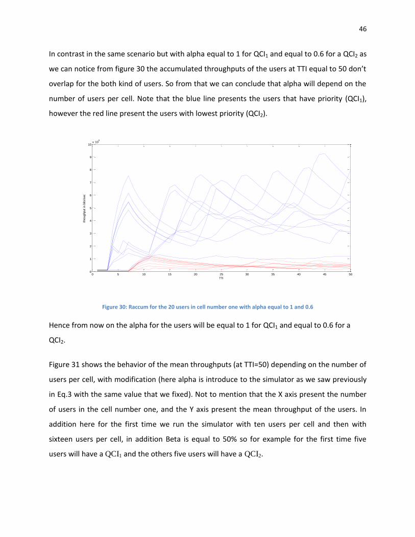
46

In contrast in the same scenario but with alpha equal to 1 for QCI1 and equal to 0.6 for a QCI2 as

we can notice from figure 30 the accumulated throughputs of the users at TTI equal to 50 don’t

overlap for the both kind of users. So from that we can conclude that alpha will depend on the

number of users per cell. Note that the blue line presents the users that have priority (QCI1),

however the red line present the users with lowest priority (QCI2).

Figure 30: Raccum for the 20 users in cell number one with alpha equal to 1 and 0.6

Hence from now on the alpha for the users will be equal to 1 for QCI1 and equal to 0.6 for a

QCI2.

Figure 31 shows the behavior of the mean throughputs (at TTI=50) depending on the number of

users per cell, with modification (here alpha is introduce to the simulator as we saw previously

in Eq.3 with the same value that we fixed). Not to mention that the X axis present the number

of users in the cell number one, and the Y axis present the mean throughput of the users. In

addition here for the first time we run the simulator with ten users per cell and then with

sixteen users per cell, in addition Beta is equal to 50% so for example for the first time five

users will have a QCI1 and the others five users will have a QCI2.

0 5 10 15 20 25 30 35 40 45 500

1

2

3

4

5

6

7

8

9

10x 10

6

TTI

thro

ughput

in b

its/s

ec

47

Figure 31: Mean throughput of the two kinds of users with alpha fix equal to 1 and 0.6

As we can notice by introducing an alpha to the simulator we just got two values for the

average user throughputs in each case, for example in case where we have ten user per cell the

five users that have QCI1 equal to one will have a mean throughput equal to 7640000 bit/s

which is highest then the mean throughput of the others five users (which has a QCI2 equal to

six) which is equal to 1002000 bit/s. The gap between the two kinds of users where we have 10

users per cell is 7.62 times, however the gap between the two kinds of users where we have 16

users per cell is 13.6, finally the gap between the two kinds of users where we have 20 users

per cell is 10.18 times.

However figure 32 shows the behavior of the mean throughputs of the users where

prioritization is not enforced (alpha equals one for both QCIs) in eq.3. Not to mention that here

also we fix the number of users per cell as follow: ten users, sixteen users per cell and finally

twenty users per cell, at TTI=50.

As we can notice there is no distinction between the average user throughputs of the users

which are in the same cell.

10 11 12 13 14 15 16 17 18 19 200

1

2

3

4

5

6

7

8x 10

6

Number of users per cell

thro

ughput

in b

its/s

ec

QCI1

QCI2

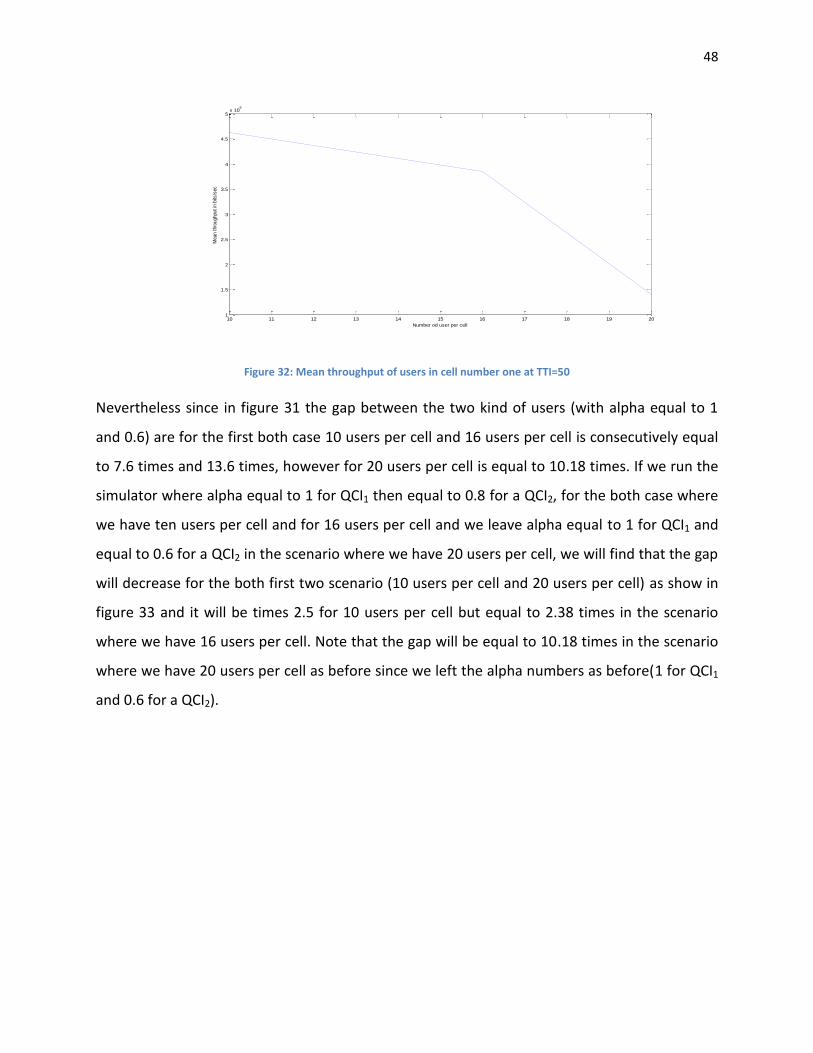
48

Figure 32: Mean throughput of users in cell number one at TTI=50

Nevertheless since in figure 31 the gap between the two kind of users (with alpha equal to 1

and 0.6) are for the first both case 10 users per cell and 16 users per cell is consecutively equal

to 7.6 times and 13.6 times, however for 20 users per cell is equal to 10.18 times. If we run the

simulator where alpha equal to 1 for QCI1 then equal to 0.8 for a QCI2, for the both case where

we have ten users per cell and for 16 users per cell and we leave alpha equal to 1 for QCI1 and

equal to 0.6 for a QCI2 in the scenario where we have 20 users per cell, we will find that the gap

will decrease for the both first two scenario (10 users per cell and 20 users per cell) as show in

figure 33 and it will be times 2.5 for 10 users per cell but equal to 2.38 times in the scenario

where we have 16 users per cell. Note that the gap will be equal to 10.18 times in the scenario

where we have 20 users per cell as before since we left the alpha numbers as before(1 for QCI1

and 0.6 for a QCI2).

10 11 12 13 14 15 16 17 18 19 201

1.5

2

2.5

3

3.5

4

4.5

5x 10

6

Number od user per cell

Mean t

hro

ughput

in b

its/s

ec

49

Figure 33: Mean throughput of the two kinds of users

4.4. Conclusion:

In conclusion, by introducing an alpha to the equation (eq.3) we just separate users following

their QCI numbers and as we saw the users with highest priority will get highest throughputs

then the other users with lower priority access. In addition we saw that value of alpha depends

on the number of users per cell.

10 11 12 13 14 15 16 17 18 19 200

1

2

3

4

5

6

7

8

9x 10

6

Number of users per cell

thro

ughput

in b

its/s

ec

QCI1

QCI2

50

Chapter 5

Conclusion and Future Work In this thesis, in order to implement the prioritization to some users following their QCI

numbers in the Vienna LTE simulator more specific in the System Level simulator since the

performance of a whole network is analyzed, first we explained the prioritization capabilities in

LTE networks and then we see the Vienna LTE simulators which is used to test and optimize

algorithms and procedure.

Since we just modify the PropSunFair scheduler it will be better to work the prioritization

capabilities in all the scheduler available in the LTE system since the scheduler allocates

resource blocks to the users and each scheduler works in different manner then the other one,

in addition it is better to work in more complex scenarios for example higher number of users,

higher number of cells and eNodeB’s, or finally to see the packet delay related to each users

when QoS is introduced.

51

References:

[1]. LTE Network Infrastructure and Elements (LTE encyclopedia); https://sites.google.com/site/lteencyclopedia/lte-network-infrastructure-and-elements

[2]. Chapter 4 Long Term Evolution (Professor Ramon Ferrus (UPC))

[3]. Policies for Public Safety Use of Commercial commercial Wireless Networks by Ryan Hallahan and Jon M.Peha, Carnegie Mellon University, October 2010; http://users.ece.cmu.edu/~peha/public_safety_priority_access.pdf

[4]. Priority access for public safety on shared commercial LTE networks, Published in Telecom World (ITU WT), 2011 Technical Symposium at ITU, 24-27 October 2011; http://ieeexplore.ieee.org/xpl/articleDetails.jsp?arnumber=6100939

[5]. Priority and QoS in the Nationwide Public Safety Broadband Network - NPSTC, April 17 2012; http://www.npstc.org/download.jsp?tableId=37&column=217&id=2304&file=PriorityAndQoSDefinition_v1_0_clean.pdf

[6]. System Level Simulation Of LTE Networks, Vienna University of Technology;

http://publik.tuwien.ac.at/files/PubDat_184908.pdf

[7]. LTE System Level simoulator documentation, Vienna University of Technology; http://www.nt.tuwien.ac.at/fileadmin/topics/simulators/LTEsystemDoc.pdf

[8]. White paper about Maximizing LTE Performance through MIMO Optimization; http://rfsolutions.pctel.com/artifacts/MIMOWhitePaperRevB-FINAL.pdf

[9]. Frequency Reuse in OFDMA Based LTE/WIMAX System, Published: April 1,2013; http://www.infoutils.com/frequency-reuse-in-ofdma-based-ltewimax-system/

[10]. LTE Downlink System Level Simulator Package Description; http://www.nt.tuwien.ac.at/research/mobile-communications/lte-downlink-system-level-simulator/

[11]. Simulation The Long Term Evolution Physical Layer, Vienna University of Technology; http://publik.tuwien.ac.at/files/PubDat_175708.pdf

[12]. Channel Codind and Link Adaptation, by Sharam Zarei, published:16 december 2009; http://www.lmk.lnt.de/fileadmin/Lehre/Seminar09/Ausarbeitungen/Ausarbeitung_Zarei.pdf

https://sites.google.com/site/lteencyclopedia/lte-network-infrastructure-and-elements

http://users.ece.cmu.edu/~peha/public_safety_priority_access.pdf

http://ieeexplore.ieee.org/xpl/articleDetails.jsp?arnumber=6100939

http://www.google.com/url?sa=t&rct=j&q=&esrc=s&source=web&cd=2&ved=0CC8QFjAB&url=http%3A%2F%2Fwww.npstc.org%2Fdownload.jsp%3FtableId%3D37%26column%3D217%26id%3D2304%26file%3DPriorityAndQoSDefinition_v1_0_clean.pdf&ei=xIp-Uo6zBqqw7AbU74CYBQ&usg=AFQjCNFXaT0z3WbngEAqg2iNzGMKfjHB4A&bvm=bv.56146854,d.d2k

http://www.npstc.org/download.jsp?tableId=37&column=217&id=2304&file=PriorityAndQoSDefinition_v1_0_clean.pdf

http://www.npstc.org/download.jsp?tableId=37&column=217&id=2304&file=PriorityAndQoSDefinition_v1_0_clean.pdf


http://www.nt.tuwien.ac.at/fileadmin/topics/simulators/LTEsystemDoc.pdf

http://rfsolutions.pctel.com/artifacts/MIMOWhitePaperRevB-FINAL.pdf

http://www.infoutils.com/frequency-reuse-in-ofdma-based-ltewimax-system/

http://www.nt.tuwien.ac.at/research/mobile-communications/lte-downlink-system-level-simulator/

http://www.nt.tuwien.ac.at/research/mobile-communications/lte-downlink-system-level-simulator/


http://www.lmk.lnt.de/fileadmin/Lehre/Seminar09/Ausarbeitungen/Ausarbeitung_Zarei.pdf

http://www.lmk.lnt.de/fileadmin/Lehre/Seminar09/Ausarbeitungen/Ausarbeitung_Zarei.pdf

52

[13]. Stefan Schwarz, Christian Mehlfuhrer and Marcus Rupp; Low Complexity Approximate

Maximum Throughput Scheduling for LTE.

performance analysis of prioritization in lte networks...

Documents