new zealand intermodal freight network and the …
TRANSCRIPT
NEW ZEALAND INTERMODAL FREIGHT NETWORK AND THE
POTENTIAL FOR MODE SHIFTING
Janice Asuncion1*, Stacy Rendall1, Dr. Rua Murray2, A/Prof. Susan Krumdieck1,
1. Department of Mechanical Engineering, University of Canterbury 2. Department of Mathematics, University of Canterbury
* Presenter
Contact: [email protected]
Office +64 3 364 2987 loc 7249
ABSTRACT
Intermodal freight transport is a system of interconnected networks involving various modes and
facilities allowing transfer of commodities from one mode to another. The system aims to provide
efficient, seamless transport of goods from the origin to its destination offering producers and
manufacturers a full range of transportation modes and routing options.
In this paper, we review the different modes of freight transportation in New Zealand as well as the
current trends of mode share. A GIS-based optimisation model is created integrating road, rail and
shipping network called the New Zealand Intermodal Freight Network (NZIFN).
The resulting model uses deterrence parameters such as operational costs and time-of-delivery as
well as energy consumption and emissions, evaluates trade-offs, and finds the most optimal route
from a given origin to a destination. The model is applied to hypothetical scenarios of distribution
from Auckland to Wellington and Auckland to Christchurch which demonstrates how freight mode
choices impact different costs associated with freight movement and the potential savings of moving
by rail or shipping.
1
I. INTRODUCTION
In New Zealand, road freight movements play an essential role in sustaining and supporting
economic growth and contribute to the quality of life of its residents. According to the New Zealand
Business Council, freight volumes would increase by 70-75% over the next 30 years if the current
growth rate continues (NZBC, 2011). An increase in road freight is tied up to gross domestic product
(GDP) growth. However, decoupling of GDP and road freight, where GDP grows at a faster rate than
road freight, is one of the holy grails in the field of the freight transportation (McKinnon, 2007).
Unfortunately for New Zealand, trends have shown that road freight volumes increase faster than
GDP growth, in particular between 1992 and 2007, decoupling was only manifested on years 2005
and 2006 (MFE, 2009). Decoupling is particularly important as it offers the prospect of economic
prosperity with reduce impact on the environment in the form of emissions. At the same time, in
light of peak oil, the sustainability of the over-reliance of New Zealand’s economy on road freight is
in question. One way to accomplish decoupling and to solve the over-reliance on fossil fuel is a shift
to less energy intensive and lower emission modes such as rail or coastal shipping (McKinnon &
Woodburn, 1996).
Modal shift requires the establishment of an intermodal freight network with transfer facilities from
one mode to another. Modelling an intermodal transport network is much more complex than a
unimodal network as each mode has its own specific characteristics with respect to infrastructure
and transport units, and operational research strategies are also needed on transfer hubs such as
finding their optimum location, allocation of capacities, and other drayage operations (Macharis &
Bontekoning 2004, Sirikijpanichkul & Ferreira, 2006).
The goal of this project is to create a visualisation tool that will look at the potential of having an
intermodal freight network with the proper infrastructures in place. A functional intermodal network
for the country requires investments to build new infrastructure and maintain existing ones, and
that the true costs of each transportation mode are factored into the model including capital
expenditures, time, maintenance, congestion and also pollution-related costs (Bolland 2010, Black
2010). However constraints on data availability will entail several assumptions concerning
infrastructures, as well as simplifying the cost-functions for modes and connectors. Through this, we
can look at the economic, environmental and energy impacts of intermodal freight transportation
and in particular assess the overall opportunities for mode-shifting of New Zealand freight.
II. REVIEW OF RELATED LITERATURE
A. Intermodal Freight Network
An intermodal network is defined as an integrated transportation system consisting of two or more
unimodal networks. Each network is composed of a set of points, called nodes, and a set of point
connectors called segments. Just in the case of unimodal systems, network optimisation models are
also utilised in intermodal freight transport logistics (Crainic & Laporte, 1997). These models are
used to find the optimal routes with cost or deterrence function given usually by distance, actual
operational costs of transport and time-of-delivery. GIS is a computer system used to analyse, store,
manage and graphically present a database with spatial components. In particular, ArcGIS, a GIS
software produced by the Environmental Systems Research Institute’s (ESRI) has a built-in Network
Analyst tool that uses shortest-path algorithms to solve the most optimal routes.
2
Several researchers have utilised the capabilities of GIS to construct intermodal freight networks
(Boile 2000, Standifer & Walton 2000, Southworth & Peterson 2000). The interdisciplinary team
from Rochester Institute of Technology developed the Geospatial Intermodal Freight Network (GIFT)
using ArcGIS 9.3 to create an intermodal network model connecting highway, rail, and shipping
networks through ports, railyards and other transfer facilities in the United States and Canada
(Winebreak et al, 2008). The main distinction of the GIFT model from other GIS-based models is the
inclusion of energy and environmental attributes on each segment of the intermodal network.
Energy costs are measured as British thermal unit per Twenty-foot-equivalent unit-mile travelled or
(BTU/TEU-mi). The emission attribute is measured in terms of different pollutants (grams/TEU-mi)
including carbon dioxide [CO2], carbon monoxide [CO], particulate matter [PM10], nitrogen oxides
[NOx], and sulphur oxides [SOx] (Winebreak 2008, Comer et al 2010).
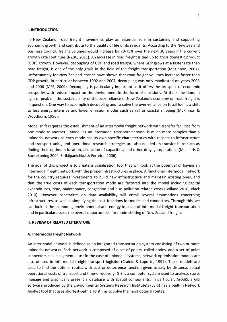
The GIFT model uses a hub-and-spoke approach in order to form a connection between the three
modal networks. Network segments refer to actual and existing network datasets in the United
States and Canada. Network spokes are artificial connections created to connect the 3 modal
networks and represent transfer facilities. The hub-and-spoke approach connects modes directly
through facilities using a Python-based ArcGIS script that builds an artificial link between appropriate
modal networks and transfer facilities. These spokes are artificial because they may not follow a
physical connection (such as a road) but instead are used as proxy for transfer paths. To make a
realistic scenario, transfer penalties are applied to all of the spokes to represent costs, energy use,
time delays, and emissions associated with intermodal transfers. These penalties are integrated into
the overall optimisation calculations so that they are incorporated in route determination.
B. Freight Flows in New Zealand:
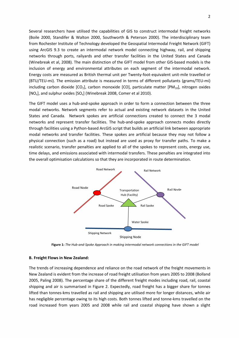
The trends of increasing dependence and reliance on the road network of the freight movements in
New Zealand is evident from the increase of road freight utilisation from years 2005 to 2008 (Bolland
2005, Paling 2008). The percentage share of the different freight modes including road, rail, coastal
shipping and air is summarised in Figure 2. Expectedly, road freight has a bigger share for tonnes
lifted than tonnes-kms travelled as rail and shipping are utilised more for longer distances, while air
has negligible percentage owing to its high costs. Both tonnes lifted and tonne-kms travelled on the
road increased from years 2005 and 2008 while rail and coastal shipping have shown a slight
Figure 1: The Hub-and-Spoke Approach in making intermodal network connections in the GIFT model
Transportation
Hub (Facility)
Road Node Rail Node
Shipping Node
Road Network
Rail Network
Shipping Network
Road Spoke Rail Spoke
Water Spoke
3
decreased. Road will remain the dominant mode for freight transport in the foreseeable future and
only up to 7% of road freight may be shifted to rail (NZBC, 2011).
Figure 2: Summary of Freight Task by Mode for years 2005 and 2008
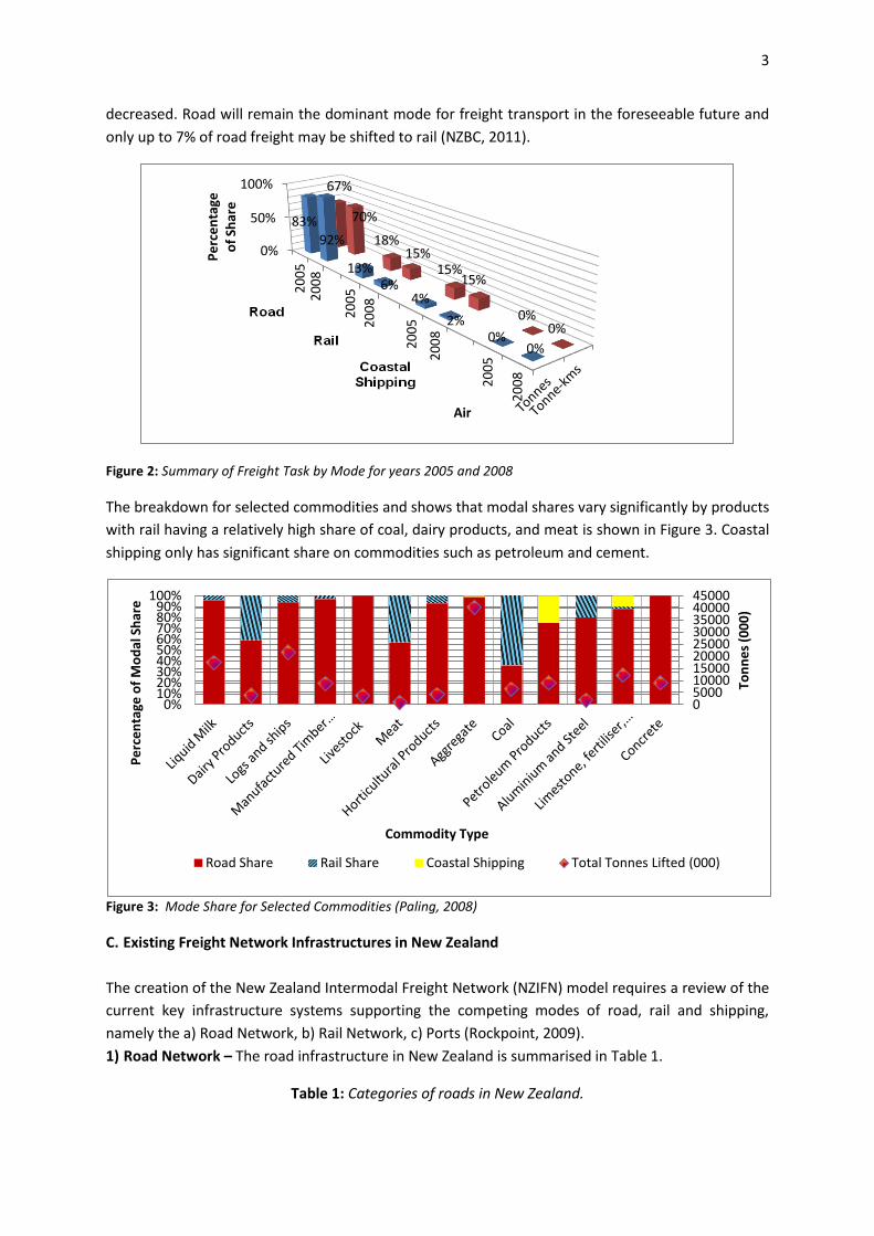
The breakdown for selected commodities and shows that modal shares vary significantly by products
with rail having a relatively high share of coal, dairy products, and meat is shown in Figure 3. Coastal
shipping only has significant share on commodities such as petroleum and cement.
Figure 3: Mode Share for Selected Commodities (Paling, 2008)
C. Existing Freight Network Infrastructures in New Zealand
The creation of the New Zealand Intermodal Freight Network (NZIFN) model requires a review of the
current key infrastructure systems supporting the competing modes of road, rail and shipping,
namely the a) Road Network, b) Rail Network, c) Ports (Rockpoint, 2009).
1) Road Network – The road infrastructure in New Zealand is summarised in Table 1.
Table 1: Categories of roads in New Zealand.
0%
50%
100%
20
05
2
00
8
20
05
20
08
20
05
20
08
20
05
20
08
83%
92%
13% 6%
4%
2% 0%
0%
67%
70%
18% 15%
15% 15%
0% 0%
Pe
rce
nta
ge
of
Shar
e
Air
0 5000 10000 15000 20000 25000 30000 35000 40000 45000
0% 10% 20% 30% 40% 50% 60% 70% 80% 90%
100%
Ton
ne
s (0
00
)
Pe
rce
nta
ge o
f M
od
al S
har
e
Commodity Type
Road Share Rail Share Coastal Shipping Total Tonnes Lifted (000)

4
Categories Total Length Percentage of Total Percentage of Vehicle-kms travelled
State Highways 11,000 km 12% 50%
Local Roads 83,000 km 88% 50%
Aside from the network itself, other road services such as drayage operations provide the essential
intermodal components for rail, international and coastal shipping movements.
2. Rail Network – The utilisation of New Zealand rail network is summarised in Table 2.
Table 2: New Zealand Rail Network Utilisation
Freight Route Freight Services Per Day
Line Capacity Utilised
Gross Tonnage
% North Bound
% South Bound
Auckland- Wellington – Christchurch
8 77% 2,870,231 43% 57%
Auckland - Tauranga
13 80% 3,588,084 61% 39%
Christchurch – Dunedin – Invercargill
9 75% 1,840,299 56% 44%
% East Bound % West Bound
West Coast – Christchurch
11 51% 2,468,958 99% 1%
Hawkes Bay Taranaki
13 60% 850,072 16% 84%
Other Lines 3,839,191
New Zealand rail infrastructure has suffered from significant underinvestment problems. In 2008
only 4,000 km of rail tracks exist to service both freight and passenger operations down from 5,689
km in 1953 (Rockpoint, 2008). Rail operations are impacted by the age, design and condition of the
country’s rail infrastructure. New Zealand’s rail system operates for the most part with an 18 tonne
maximum axle load whereas world standards are 25 tonnes per axle load. Bridges, tunnel clearances
and steep gradients in the network restrict the weight, height and speed of rail freight. While recent
investment has targeted key areas of restriction, bridges remain a major network issue and until
addressed, track upgrades elsewhere are unable to be fully utilised (Rockpoint, 2008).
3. Coastal shipping – New Zealand is currently serviced by 16 key ports and summarised in Table 3.
Table 3: New Zealand key ports (Rockpoint, 2008)
Port Location/City, Region Container Terminal
Port Type
North Port Marsden Point, Whangarei, Northland
No Bulk
Ports of Auckland Waitemata Harbour, Auckland Yes International
Ports of Auckland Onehunga (Manukau Harbour), Auckland
No Coastal
Ports of Tauranga Sulphur Point, Mt Maunganui, Bay of Plenty
Yes International
Eastland Port Gisborne, Poverty Bay No Bulk
Port Taranaki New Plymouth, Taranaki Yes Bulk
5
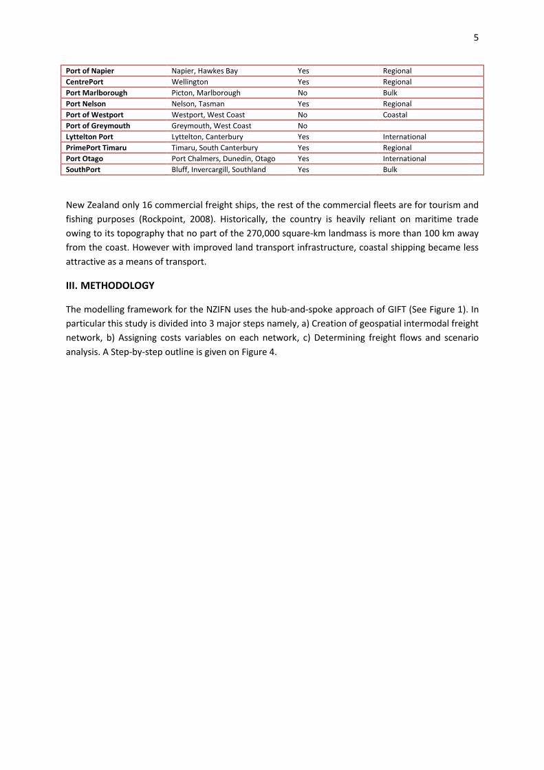
Port of Napier Napier, Hawkes Bay Yes Regional
CentrePort Wellington Yes Regional
Port Marlborough Picton, Marlborough No Bulk
Port Nelson Nelson, Tasman Yes Regional
Port of Westport Westport, West Coast No Coastal
Port of Greymouth Greymouth, West Coast No
Lyttelton Port Lyttelton, Canterbury Yes International
PrimePort Timaru Timaru, South Canterbury Yes Regional
Port Otago Port Chalmers, Dunedin, Otago Yes International
SouthPort Bluff, Invercargill, Southland Yes Bulk
New Zealand only 16 commercial freight ships, the rest of the commercial fleets are for tourism and
fishing purposes (Rockpoint, 2008). Historically, the country is heavily reliant on maritime trade
owing to its topography that no part of the 270,000 square-km landmass is more than 100 km away
from the coast. However with improved land transport infrastructure, coastal shipping became less
attractive as a means of transport.
III. METHODOLOGY
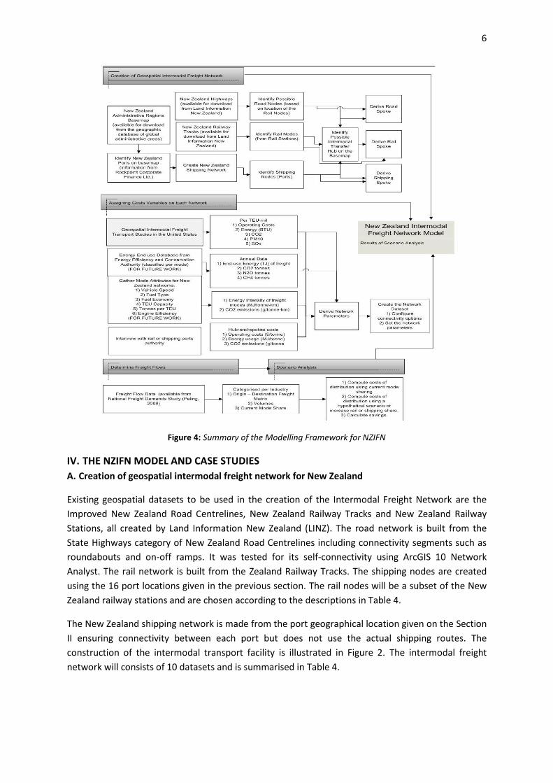
The modelling framework for the NZIFN uses the hub-and-spoke approach of GIFT (See Figure 1). In
particular this study is divided into 3 major steps namely, a) Creation of geospatial intermodal freight
network, b) Assigning costs variables on each network, c) Determining freight flows and scenario
analysis. A Step-by-step outline is given on Figure 4.
6
Figure 4: Summary of the Modelling Framework for NZIFN
IV. THE NZIFN MODEL AND CASE STUDIES
A. Creation of geospatial intermodal freight network for New Zealand
Existing geospatial datasets to be used in the creation of the Intermodal Freight Network are the
Improved New Zealand Road Centrelines, New Zealand Railway Tracks and New Zealand Railway
Stations, all created by Land Information New Zealand (LINZ). The road network is built from the
State Highways category of New Zealand Road Centrelines including connectivity segments such as
roundabouts and on-off ramps. It was tested for its self-connectivity using ArcGIS 10 Network
Analyst. The rail network is built from the Zealand Railway Tracks. The shipping nodes are created
using the 16 port locations given in the previous section. The rail nodes will be a subset of the New
Zealand railway stations and are chosen according to the descriptions in Table 4.
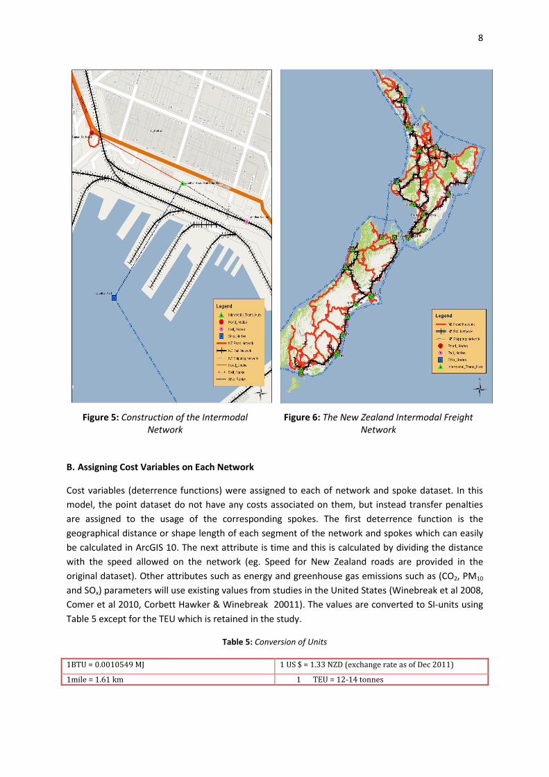
The New Zealand shipping network is made from the port geographical location given on the Section
II ensuring connectivity between each port but does not use the actual shipping routes. The
construction of the intermodal transport facility is illustrated in Figure 2. The intermodal freight
network will consists of 10 datasets and is summarised in Table 4.
7
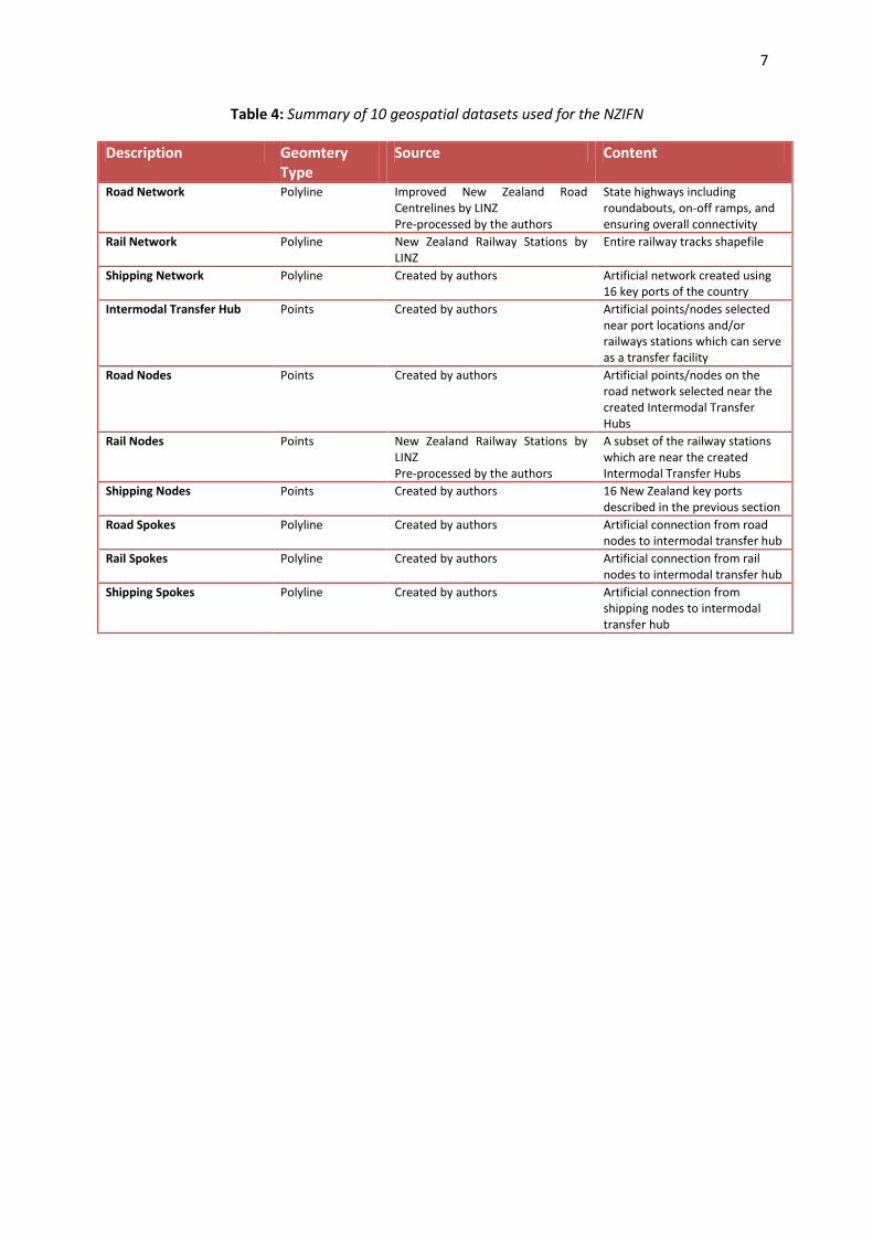
Table 4: Summary of 10 geospatial datasets used for the NZIFN
Description Geomtery Type
Source Content
Road Network Polyline Improved New Zealand Road Centrelines by LINZ Pre-processed by the authors
State highways including roundabouts, on-off ramps, and ensuring overall connectivity
Rail Network Polyline New Zealand Railway Stations by LINZ
Entire railway tracks shapefile
Shipping Network Polyline Created by authors Artificial network created using 16 key ports of the country
Intermodal Transfer Hub Points Created by authors Artificial points/nodes selected near port locations and/or railways stations which can serve as a transfer facility
Road Nodes Points Created by authors Artificial points/nodes on the road network selected near the created Intermodal Transfer Hubs
Rail Nodes Points New Zealand Railway Stations by LINZ Pre-processed by the authors
A subset of the railway stations which are near the created Intermodal Transfer Hubs
Shipping Nodes Points Created by authors 16 New Zealand key ports described in the previous section
Road Spokes Polyline Created by authors Artificial connection from road nodes to intermodal transfer hub
Rail Spokes Polyline Created by authors Artificial connection from rail nodes to intermodal transfer hub
Shipping Spokes Polyline Created by authors Artificial connection from shipping nodes to intermodal transfer hub
8
Figure 5: Construction of the Intermodal Network
Figure 6: The New Zealand Intermodal Freight Network
B. Assigning Cost Variables on Each Network
Cost variables (deterrence functions) were assigned to each of network and spoke dataset. In this
model, the point dataset do not have any costs associated on them, but instead transfer penalties
are assigned to the usage of the corresponding spokes. The first deterrence function is the
geographical distance or shape length of each segment of the network and spokes which can easily
be calculated in ArcGIS 10. The next attribute is time and this is calculated by dividing the distance
with the speed allowed on the network (eg. Speed for New Zealand roads are provided in the
original dataset). Other attributes such as energy and greenhouse gas emissions such as (CO2, PM10
and SOx) parameters will use existing values from studies in the United States (Winebreak et al 2008,
Comer et al 2010, Corbett Hawker & Winebreak 20011). The values are converted to SI-units using
Table 5 except for the TEU which is retained in the study.
Table 5: Conversion of Units
1BTU = 0.0010549 MJ 1 US $ = 1.33 NZD (exchange rate as of Dec 2011)
1mile = 1.61 km 1 TEU = 12-14 tonnes
9
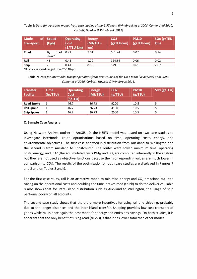
Table 6: Data for transport modes from case studies of the GIFT team (Winebreak et al 2008, Comer et al 2010,
Corbett, Hawker & Winebreak 2011)
Mode of Transport
Speed (kph)
Operating Cost ($/TEU-km)
Energy (MJ/TEU-km)
CO2 (g/TEU-km)
PM10 (g/TEU-km)
SOx (g/TEU-km)
Road By road class*
0.71 7.01 661.74 0.07 0.14
Rail 45 0.45 1.70 124.84 0.06 0.02
Ship 25 0.41 8.55 679.5 0.61 2.07 *Road class speed ranged from 20-110kph
Table 7: Data for intermodal transfer penalties from case studies of the GIFT team (Winebreak et al 2008,
Comer et al 2010, Corbett, Hawker & Winebreak 2011)
Transfer Facility
Time (hr/TEU)
Operating Cost ($/TEU)
Energy (MJ/TEU)
CO2 (g/TEU)
PM10 (g/TEU)
SOx (g/TEU)
Road Spoke 1 46.7 26.73 9200 10.5 5
Rail Spoke 1 46.7 26.73 4100 10.5 5
Ship Spoke 1 46.7 26.73 2500 10.5 5
C. Sample Case Analysis
Using Network Analyst toolset in ArcGIS 10, the NZIFN model was tested on two case studies to
investigate intermodal route optimisations based on time, operating costs, energy, and
environmental objectives. The first case analysed is distribution from Auckland to Wellington and
the second is from Auckland to Christchurch. The routes were solved minimum time, operating
costs, energy, and CO2 (the accumulated costs PM10 and SOx are computed inherently in the analysis
but they are not used as objective functions because their corresponding values are much lower in
comparison to CO2). The results of the optimisation on both case studies are displayed in Figures 7
and 8 and on Tables 8 and 9.
For the first case study, rail is an attractive mode to minimise energy and CO2 emissions but little
saving on the operational costs and doubling the time it takes road (truck) to do the deliveries. Table
8 also shows that for intra-island distribution such as Auckland to Wellington, the usage of ship
performs poorly on all accounts.
The second case study shows that there are more incentives for using rail and shipping, probably
due to the longer distances and the inter-island transfer. Shipping provides low-cost transport of
goods while rail is once again the best mode for energy and emissions-savings. On both studies, it is
apparent that the only benefit of using road (trucks) is that it has lower total than other modes.

10
Figure 7: Scenario Analysis of Distribution from
Auckland to Wellington
Figure 8: Scenario Analysis of Distribution from Auckland to Christchurch
Table 8: Results for optimisation model runs from Auckland to Wellington
Route Primary Mode
Total Time (hr)
Total Operational Costs ($)
Total Energy (MJ)
Total CO2 (g)
Total PM10 (g)
Total SOx(g)
Min Time
Road 7 462 4496 425,463 46 90
Min Operational Costs, Energy, CO2
Rail 17 419 1215 100,703 66 26
Forcing Ship Route
Ship 34 423 5812 470,972 441 1400
Table 9: Results for optimisation model runs from Auckland to Christchurch
Route Primary Mode
Total Time (hr)
Total Operational Costs ($)
Total Energy (MJ)
Total CO2 (g)
Total PM10 (g)
Total SOx(g)
Min Time
Road 21 917 8302 772,955 197 470
Min Operational
Ship 45 570 7945 648,342 593 1887
11
Costs
Min Energy, CO2
Rail 37 867 3268 271,436 231 373
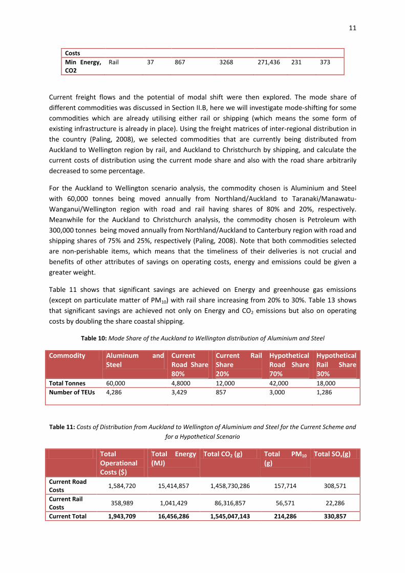
Current freight flows and the potential of modal shift were then explored. The mode share of
different commodities was discussed in Section II.B, here we will investigate mode-shifting for some
commodities which are already utilising either rail or shipping (which means the some form of
existing infrastructure is already in place). Using the freight matrices of inter-regional distribution in
the country (Paling, 2008), we selected commodities that are currently being distributed from
Auckland to Wellington region by rail, and Auckland to Christchurch by shipping, and calculate the
current costs of distribution using the current mode share and also with the road share arbitrarily
decreased to some percentage.
For the Auckland to Wellington scenario analysis, the commodity chosen is Aluminium and Steel
with 60,000 tonnes being moved annually from Northland/Auckland to Taranaki/Manawatu-
Wanganui/Wellington region with road and rail having shares of 80% and 20%, respectively.
Meanwhile for the Auckland to Christchurch analysis, the commodity chosen is Petroleum with
300,000 tonnes being moved annually from Northland/Auckland to Canterbury region with road and
shipping shares of 75% and 25%, respectively (Paling, 2008). Note that both commodities selected
are non-perishable items, which means that the timeliness of their deliveries is not crucial and
benefits of other attributes of savings on operating costs, energy and emissions could be given a
greater weight.
Table 11 shows that significant savings are achieved on Energy and greenhouse gas emissions
(except on particulate matter of PM10) with rail share increasing from 20% to 30%. Table 13 shows
that significant savings are achieved not only on Energy and CO2 emissions but also on operating
costs by doubling the share coastal shipping.
Table 10: Mode Share of the Auckland to Wellington distribution of Aluminium and Steel
Commodity Aluminum and Steel
Current Road Share 80%
Current Rail Share 20%
Hypothetical Road Share 70%
Hypothetical Rail Share 30%
Total Tonnes 60,000 4,8000 12,000 42,000 18,000
Number of TEUs 4,286
3,429
857 3,000 1,286
Table 11: Costs of Distribution from Auckland to Wellington of Aluminium and Steel for the Current Scheme and
for a Hypothetical Scenario
Total Operational Costs ($)
Total Energy (MJ)
Total CO2 (g) Total PM10 (g)
Total SOx(g)
Current Road Costs
1,584,720 15,414,857 1,458,730,286 157,714 308,571
Current Rail Costs
358,989 1,041,429 86,316,857 56,571 22,286
Current Total 1,943,709 16,456,286 1,545,047,143 214,286 330,857
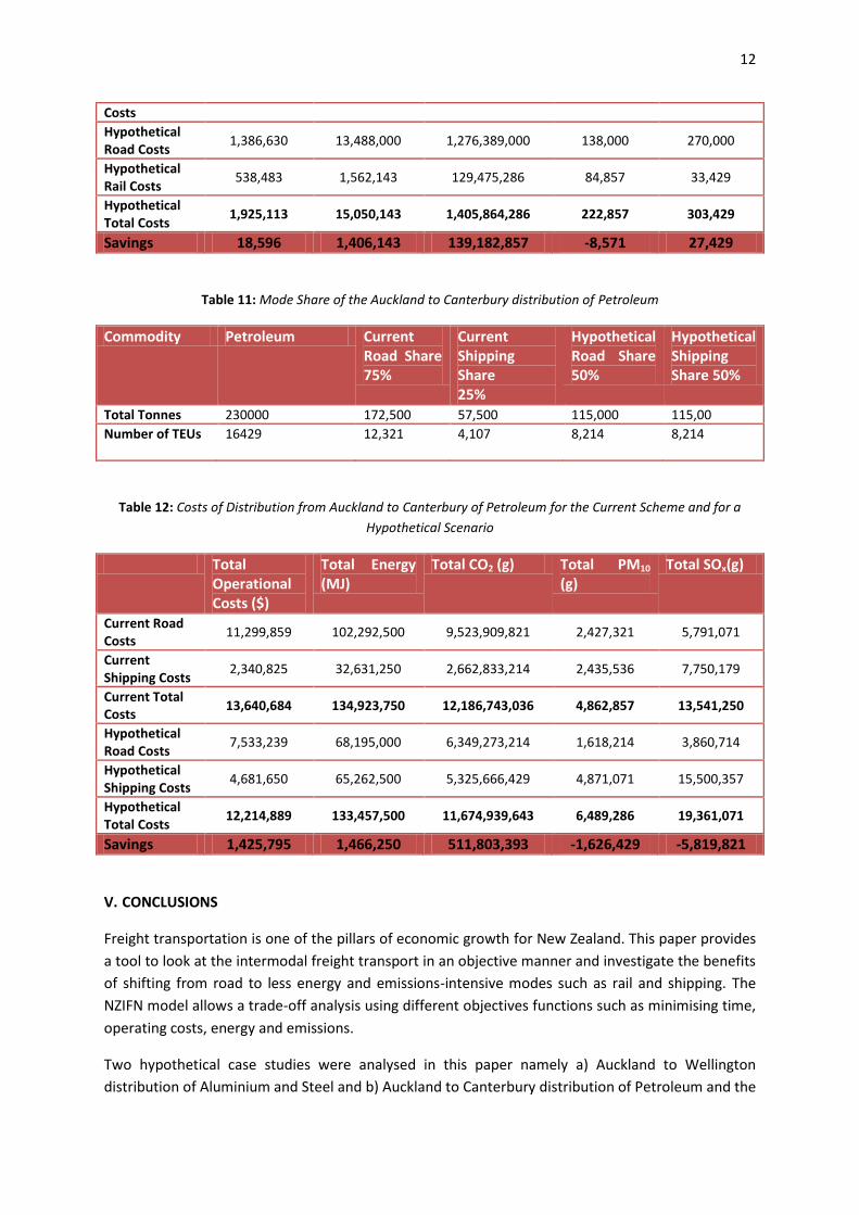
12
Costs
Hypothetical Road Costs
1,386,630 13,488,000 1,276,389,000 138,000 270,000
Hypothetical Rail Costs
538,483 1,562,143 129,475,286 84,857 33,429
Hypothetical Total Costs
1,925,113 15,050,143 1,405,864,286 222,857 303,429
Savings 18,596 1,406,143 139,182,857 -8,571 27,429
Table 11: Mode Share of the Auckland to Canterbury distribution of Petroleum
Commodity Petroleum Current Road Share 75%
Current Shipping Share 25%
Hypothetical Road Share 50%
Hypothetical Shipping Share 50%
Total Tonnes 230000 172,500 57,500 115,000 115,00
Number of TEUs 16429
12,321 4,107 8,214 8,214
Table 12: Costs of Distribution from Auckland to Canterbury of Petroleum for the Current Scheme and for a
Hypothetical Scenario
Total Operational Costs ($)
Total Energy (MJ)
Total CO2 (g) Total PM10 (g)
Total SOx(g)
Current Road Costs
11,299,859 102,292,500 9,523,909,821 2,427,321 5,791,071
Current Shipping Costs
2,340,825 32,631,250 2,662,833,214 2,435,536 7,750,179
Current Total Costs
13,640,684 134,923,750 12,186,743,036 4,862,857 13,541,250
Hypothetical Road Costs
7,533,239 68,195,000 6,349,273,214 1,618,214 3,860,714
Hypothetical Shipping Costs
4,681,650 65,262,500 5,325,666,429 4,871,071 15,500,357
Hypothetical Total Costs
12,214,889 133,457,500 11,674,939,643 6,489,286 19,361,071
Savings 1,425,795 1,466,250 511,803,393 -1,626,429 -5,819,821
V. CONCLUSIONS
Freight transportation is one of the pillars of economic growth for New Zealand. This paper provides
a tool to look at the intermodal freight transport in an objective manner and investigate the benefits
of shifting from road to less energy and emissions-intensive modes such as rail and shipping. The
NZIFN model allows a trade-off analysis using different objectives functions such as minimising time,
operating costs, energy and emissions.
Two hypothetical case studies were analysed in this paper namely a) Auckland to Wellington
distribution of Aluminium and Steel and b) Auckland to Canterbury distribution of Petroleum and the
13
computations for both studies showed the potential savings of shifting a fraction of the total
commodities moved from road to rail or shipping. The calculations showed significant Energy and
CO2 emissions-savings and even reduced operating costs. Both of the commodities chosen were non-
perishable and hence timeliness of deliveries may be traded for energy and emissions benefits
particularly as fuel supply decreases and emission reduction schemes raise the relative costs of
trucking.
The results of the hypothetical analysis could be useful for policy-makers in decision-making process
concerning proper investments for a sustainable freight system for New Zealand. By investing on
infrastructures that would aid in the creation of an intermodal freight system for New Zealand, it is
possible to build a system more resilient to rising fuel prices and reduce environment impact.
VI. RECOMMENDATIONS
The NZIFN model used in the scenario analysis is based uponcosts parameters from the United
States study (Winebreak et al 2008, Comer et al 2010, Corbett, Hawker & Winebreak 2011). As a
future work, it will be possible to utilise New Zealand-based data such as that provided by the
Energy Efficiency and Conservation Authority for the deterrence parameters on the road, rail and
shipping networks. Also, it is recommended to interview and survey port and transfer facilities to
look at the transfer penalties for existing hubs-and-spokes in New Zealand.
The next step is to investigate the risk exposure of the current distribution scheme to constraints on
the oil-supply and cap on emissions.
ACKNOWLEDGEMENTS:
This work is supported under Contract C01X0903, Towards Sustainable Urban Forms, National
Institute of Water and Atmospheric Research Ltd. (NIWA). The authors would also like to
acknowledge the help of Dr. Shannon Page for the useful suggestions in freight energy usage.
REFERENCES:
BLACK W. 2010. Sustainable Transport: Problems and Solutions. The Guilford Press, London.
BOILE M. 2000. Intermodal Transportation Network Analysis – A GIS Application. Paper presented at
the 10th Mediterranean Electrotechnical Conference.
BOLLAND J. 2005 Development of a New Zealand National Freight Matrix. Technical Report. Land
Transport New Zealand.
BOLLAND J. 2010. Independent Advice on the Economic Costs and Benefits of Rail Freight Stage 3.
Final Report from Ministry of Transport.
14
COMER B. et al. 2010. Marine Vessels as Substitutes for Heavy-Duty Trucks in Great Lakes Freight
Transportation. Journal of the Air and Waste Management Association.
CORBETT J., HAWKER J. & WINEBREAK J. 2011. Evaluating the Environmental Attributes of Freight
Traffic along the U.S. West Coast. ARB Air Pollution Seminar Series, University of Delaware.
CRAINIC T. & LAPORT G. 1997 Planning models for freight transportation. European Journal of
Operational Research (97).
MACHARIS C. & BONTEKONING Y. 2004. Opportunities for OR in Intermodal Freight Transport
Research: A review. European Journal of Operational Research, 153.
McKINNON A. & WOODBURN A. 1996. Logistical Restructuring and Road Freight Traffic Growth.
Transportation 23.
McKINNON A. 2007. Decoupling of road freight transport and economic growth trends in the UK: An
exploratory analysis, Transport Reviews (27).
MFE. 2009. Vehicle Kilometres Travelled By Road. Ministry for Environment Technical Report.
NZBC. 2011. Future Freight Solutions: An Agenda for Action. Technical Report from the New Zealand
Business Council for Sustainable Development.
PALING R. 2008. National Freight Demands Study. Technical Report. Ministry of Transport and New
Zealand Transport Agency.
ROCKPOINT. 2009. Coastal shipping and modal freight choice. Technical Report, Rockpoint Corporate
Finance Ltd. NZTA.
SIRIKIJPANICHKUL A. & FERREIRA L. 2006. Modeling Intermodal Freight Hub Location Decisions. IEEE
International Conference on Systems, Man, and Cybernetics.
SOUTHWORTH F. & PETERSON B. 2000. Intermodal and International Freight Network Modeling.
Geographic Information Systems in Transportation Research. Amsterdam, Netherlands.
STANDIFER G. & WALTON C. 2000. Development of a GIS model for Intermodal Freight. Austin
Texas: Southwest Regional University Transportation Center.
WINEBREAK J. et al. 2008. Assessing energy, environmental, and economic tradeoffs on intermodal
freight transportation. Journal of the Air and Waste Management Association.