Discu

ssionPaper

|Discu

ssionPaper

|Discu

ssionPaper

|Discu

ssionPaper

|

Manuscript prepared for Atmos. Chem. Phys. Discuss.with version 2014/09/16 7.15 Copernicus papers of the LATEX class copernicus.cls.Date: 13 October 2015

On the ability of RegCM4 regional climatemodel to simulate surface solar radiationpatterns over Europe: an assessment usingsatellite-based observationsG. Alexandri1,2, A. K. Georgoulias3,4,5, P. Zanis3, E. Katragkou3, A. Tsikerdekis3,K. Kourtidis2, and C. Meleti1

1Laboratory of Atmospheric Physics, Physics Department, Aristotle University of Thessaloniki,54124, Thessaloniki, Greece2Laboratory of Atmospheric Pollution and Pollution Control Engineering of Atmospheric Pollutants,School of Engineering, Democritus University of Thrace, 67100, Xanthi, Greece3Department of Meteorology and Climatology, School of Geology, Aristotle University ofThessaloniki, Thessaloniki, 54124, Greece4Multiphase Chemistry Department, Max Planck Institute for Chemistry, 55128,Mainz, Germany5Energy, Environment and Water Research Center, The Cyprus Institute, Nicosia, Cyprus

Correspondence to: G. Alexandri (alexang@auth.gr)

1

Discu

ssionPaper

|Discu

ssionPaper

|Discu

ssionPaper

|Discu

ssionPaper

|

Abstract

In this work, we assess the ability of RegCM4 regional climate model to simulate surfacesolar radiation (SSR) patterns over Europe. A decadal RegCM4 run (2000–2009) was im-plemented and evaluated against satellite-based observations from the Satellite ApplicationFacility on Climate Monitoring (CM SAF) showing that the model simulates adequately the5

SSR patterns over the region. The SSR bias between RegCM4 and CM SAF is +1.5 % forMFG (Meteosat First Generation) and +3.3 % for MSG (Meteosat Second Generation) ob-servations. The relative contribution of parameters that determine the transmission of solarradiation within the atmosphere to the deviation appearing between RegCM4 and CM SAFSSR is also examined. Cloud macrophysical and microphysical properties such as cloud10

fractional cover (CFC), cloud optical thickness (COT) and cloud effective radius (Re) fromRegCM4 are evaluated against data from CM SAF. The same procedure is repeated foraerosol optical properties such as aerosol optical depth (AOD), asymmetry factor (ASY)and single scattering albedo (SSA), as well as other parameters including surface broad-band albedo (ALB) and water vapor amount (WV) using data from MACv1 aerosol clima-15

tology, from CERES satellite sensors and from ERA-Interim reanalysis. It is shown herethat the good agreement between RegCM4 and satellite-based SSR observations can bepartially attributed to counteracting effects among the above mentioned parameters. Thecontribution of each parameter to the RegCM4-CM SAF SSR deviations is estimated withthe combined use of the aforementioned data and a radiative transfer model (SBDART).20

CFC, COT and AOD are the major determinants of these deviations on a monthly basis;however, the other parameters also play an important role for specific regions and seasons.Overall, for the European domain, the underestimation of CFC by RegCM4 is the mostimportant cause of the SSR overestimation on an annual basis.

2

Discu

ssionPaper

|Discu

ssionPaper

|Discu

ssionPaper

|Discu

ssionPaper

|

1 Introduction

Modeling climate on a regional scale is essential for assessing the impact of climate changeon society, economy and natural resources. Regional climate models are limited-area mod-els that simulate climate processes being often used to downscale dynamically global modelsimulations or global reanalysis data for specific regions in order to provide more detailed5

results (Laprise, 2008; Rummukainen, 2010). Several studies suggest that we can benefitfrom the use of regional climate models, especially due to the higher resolution of station-ary features like topography, coastlines and from the improved representation of small-scaleprocesses such as convective precipitation (see Flato et al., 2013, and references therein).Usually, regional climate models are evaluated and “tuned” according to their ability to sim-10

ulate temperature and precipitation (e.g. Giorgi et al., 2012; Vautard et al., 2013; Kotlarskiet al., 2014). However, as discussed in Katragkou et al. (2015), the role of other climatolog-ical parameters should be included in the evaluation procedure of regional climate models.

For example, the ability of regional climate models to assess surface solar radiation (SSR)patterns has not received so much attention despite the fact that SSR plays a core role in15

various climatic processes and parameters such as: (1) evapotranspiration (e.g. Teulinget al., 2009), (2) hydrological cycle (e.g. Allen and Ingram, 2002; Ramanathan et al., 2001;Wang et al., 2010; Wild and Liepert, 2010), (3) photosynthesis (e.g. Gu et al., 2002; Mer-cado et al., 2009), (4) oceanic heat budget (e.g. Lewis et al., 1990; Webster et al., 1996;Bodas-Salcedo et al., 2014), (5) global energy balance (e.g. Kim and Ramanathan, 2008;20

Stephens et al., 2012; Trenberth et al., 2009; Wild et al., 2013) and solar energy production(Hammer et al., 2003) and largely affects temperature and precipitation. The same standsfor the parameters that drive SSR levels, such as cloud macrophysical and microphysicalproperties (cloud fractional cover CFC, cloud optical thickness COT and cloud effective ra-dius Re), aerosol optical properties (aerosol optical depth AOD, asymmetry factor ASY and25

single scattering albedo SSA), surface broadband albedo (ALB) and atmospheric water va-por amount (WV). However, during the last years, there were a few regional climate modelstudies focusing on the SSR levels or the net surface shortwave radiation, either to examine

3

Discu

ssionPaper

|Discu

ssionPaper

|Discu

ssionPaper

|Discu

ssionPaper

|

the dimming/brightening effect (e.g. Zubler et al., 2011; Chiacchio et al., 2015) or to eval-uate the models (e.g. Jaeger et al., 2008; Markovic et al., 2008; Kothe and Ahrens, 2010;Kothe et al., 2011, 2014; Güttler et al., 2014). These studies highlight the dominating effectof cloud cover and surface albedo.

In this work, we go a step further, proceeding to a detailed evaluation of the ability of5

RegCM4 regional climate model to simulate SSR patterns over Europe taking into accountnot only CFC and ALB but also COT, Re, AOD, ASY, SSA and WV. For the scopes ofthis study, the same parameters are extracted from satellite-based observational data (CMSAF, CERES), data from an aerosol climatology (MACv1) and data from the ERA-Interimreanalysis (see Table 1). First a decadal simulation (2000–2009) is implemented with the10

model and the output is evaluated against observations from the EUMETSAT geostationarysatellites of CM SAF. SSR data from the Meteosat First Generation (MFG) satellites areavailable for the period 2000–2005 while data from the Meteosat Second Generation (MSG)satellites are available for the period 2006–2009. These data are characterized by a highspatial (∼ 3–5 km) and temporal resolution (15–30 min) and have been validated in the past,15

constituting a well-established product. In Sect. 2.1, the basic features of the model aredescribed along with the simulation setup and the way various parameters are calculatedby the model. In Sects. 2.2 and 2.3, a description of the satellite data from CM SAF andthe other data which are used for the evaluation of RegCM4 is given, while, in Sect. 2.4, wediscuss the methodology followed in this manuscript. Section 3.1 includes the evaluation20

of RegCM4 SSR against data from MFG and MSG, Sects. 3.2 and 3.3 the evaluation ofCFC, COT and Re against data from MSG, Sect. 3.4 the comparison of RegCM4 AOD,ASY and SSA with data from MACv1 aerosol climatology and Sect. 3.5 the comparison ofRegCM4 WV and ALB with data from ERA-Interim reanalysis and CERES satellite sensors,respectively. The CFC, COT, Re, AOD, ASY, SSA, ALB and WV datasets where chosen so25

as to be consistent with the CM SAF SSR dataset. The potential contribution of variousparameters to the RegCM4-CM SAF SSR differences is estimated with the combined useof the data mentioned above and a radiative transfer model for the MSG SSR period (2006–

4

Discu

ssionPaper

|Discu

ssionPaper

|Discu

ssionPaper

|Discu

ssionPaper

|

2009). The results are presented in Sect. 3.6, while the main findings of this manuscript aresummarized in Sect. 4.

2 Model description, data and methods

2.1 RegCM4 description and simulation setup

In this work, a decadal (2000–2009) simulation was implemented with RegCM4.4 (hereafter5

denoted as RegCM4 or RegCM) for the greater European region with an horizontal resolu-tion of 50 km. The model’s domain extends from 65◦ W to 65◦ E and 15 to 75◦ N includingthe largest part of the Sahara Desert and part of Middle East (see Fig. S1 in the Sup-plement of this manuscript). RegCM is a hydrostatic, sigma-p regional climate model witha dynamical core based on the hydrostatic version of NCAR-PSU’s Mesoscale Model ver-10

sion 5 (MM5) (Grell et al., 1994). Specifically, RegCM4 is a substantially improved versionof the model compared to its predecessor RegCM3 (Pal et al., 2007) by means of softwarecode and physics (e.g. radiative transfer, planetary boundary layer, convection schemesover land and ocean, land types and surface processes, ocean-air exchanges). Details onthe historical evolution of RegCM from the late 1980s until today and a full description of15

RegCM4’s basic features are given in Giorgi et al. (2012).Data from ECMWF’s ERA-Interim reanalysis were used as lateral boundary conditions.

RegCM4 through a simplified aerosol scheme accounts for anthropogenic SO2, sulfates,organic and black carbon (Solmon et al., 2006). The emissions of these anthropogenicaerosols are based on monthly, timed-dependent, historical emissions from the Coupled20

Model Intercomparison Project Phase 5 (CMIP5) (Lamarque et al., 2010) with one yearspin up time (1999). This inventory is used by a number of climate models in support of themost recent report of the Intergovernmental Panel on Climate Change (IPCC, 2013). Themodel also accounts for maritime particles through a 2-bin sea salt scheme (Zakey et al.,2008) and for dust through a 4-bin approach (Zakey et al., 2006). For our simulation, the25

MIT-Emanuel convection scheme (Emanuel, 1991; Emanuel and Zivkovic-Rothman, 1999)

5

Discu

ssionPaper

|Discu

ssionPaper

|Discu

ssionPaper

|Discu

ssionPaper

|

was used. Convection is triggered when the buoyancy level is higher than the cloud baselevel. The cloud mixing is considered episodic and inhomogenous, the convective fluxesbeing based on a model of sub-cloud-scale updrafts and downdrafts (Giorgi et al., 2012).Zanis et al. (2009) reported for RegCM3 that the low stratiform clouds are systematicallydenser and more persistent with the use of the Grell (Grell, 1993) convective scheme than5

with the Emannuel scheme, a result with major importance for the cloud- radiation feedback.The boundary layer scheme of Holtslag et al. (1990) was utilized while the Subgrid ExplicitMoisture Scheme (SUBEX) handles large-scale cloud and precipitation computations. Theocean flux scheme was taken from Zeng et al. (1998) with the Biosphere–AtmosphereTransfer Scheme (BATS) (Dickinson et al., 1993) accounting for land surface processes.10

The Community Climate Model version 3 (CCM3) (Kiehl et al., 1996) radiative packagehandles radiative transfer within RegCM4. The CCM3 scheme employs the δ-Eddingtonapproximation following its predecessor (CCM2) (Briegleb, 1992). Especially for the short-wave radiation, the radiative transfer model takes into account the effect of atmosphericwater vapor and greenhouse gasses, aerosol amount and optical properties per layer (e.g.15

aerosol optical thickness, asymmetry factor, single scattering albedo) as well as cloudmacrophysical (e.g. cloud fractional cover) and microphysical properties per layer (e.g. ef-fective droplet radius, liquid water path, cloud optical thickness) and land surface properties(surface albedo). The radiative transfer equation is solved for 18 discrete spectral intervalsfrom 0.2 to 5 µm for the 18 RegCM vertical sigma layers from 50 hPa to the surface.20

The effect of clouds on shortwave radiation is manifested by CFC, cloud droplet size andcloud water path (CWP) which is based on the prognostically calculated parameter of cloudwater amount (Giorgi et al., 2012). Within the model, the effective droplet radius for liquidclouds (Rel) is considered constant (10 µm) over the ocean while over land it is given asa function of temperature (Kiehl et al., 1998; Collins et al., 2004). On the other hand, the25

ice particle effective radius (Rei) is given as a function of normalized pressure, starting from

6

Discu

ssionPaper

|Discu

ssionPaper

|Discu

ssionPaper

|Discu

ssionPaper

|

10 µm. The equations used for the calculation of Rel and Rei are given below.

Rel =

5µm T >−10◦C

5− 5(T+1020

)µm −30◦C≤ T ≤−10◦C

Rei T <−30◦C

(1)

Rei =

Reimin p/ps > phighI

Reimin− (Reimax−Reimin)

[(p/ps)−phigh

I

phighI −plow

I

]µm p/ps ≤ phigh

I

(2)

where Reimax = 30 µm, Reimin = 10 µm, phighI = 0.4 and plow

I = 0.0. The fraction (fice) ofcloud water that consists of ice particles is given as a function of temperature (T), the5

fraction (fliq) of the liquid water droplets being calculated as fliq=1-fice.

fice =

0 T >−10◦C

−0.05(T + 10) −30◦C≤ T ≤−10◦C

1 T <−30◦C

(3)

Then, the radiative properties of liquid and ice clouds in the shortwave spectral region aregiven by the following parameterizations, originally found in Slingo (1989) and revisited byBriegleb et al. (1992).10

COTλph = CWP

[aλph +

bλph

Reph

]fph (4)

ωλph = 1− cλph− dλphReph (5)

gλph = eλph + fλphReph (6)

φλph =(gλph

)2(7)

7

Discu

ssionPaper

|Discu

ssionPaper

|Discu

ssionPaper

|Discu

ssionPaper

|

where superscript λ denotes the spectral interval and subscript ph denotes the phase (liq-uid/ice). Also, ω is the single scattering albedo, g is the asymmetry factor and φ is the phasefunction of clouds. It has to be highlighted here that all the equations presented above aregiven in Kiehl et al. (1998) and Collins et al. (2004) with a slightly different annotation. Thecoefficients a–f for liquid clouds are given in Slingo (1989), while for ice clouds in Ebert5

and Curry (1992) for the four pseudo-spectral intervals (0.25–0.69, 0.69–1.19, 1.19–2.38and 2.38–4.00 µm) employed in the radiative scheme of RegCM. Especially for COT, in thispaper we calculated it for the spectral interval 0.25–0.69 µm for both liquid and ice cloudsso as to be comparable to the CM SAF satellite retrieved COT at 0.6 µm (see Sect. 2.2).Following the approach of Cess (1985), to derive the bulk COT for the whole atmospheric10

column, the COTs calculated for each layer are simply added. The total COT for each layeris calculated by merging the COT values for liquid and ice clouds.

Within RegCM, CFC at each layer is calculated from relative humidity and cloud dropletradius. The surface radiation flux in RegCM4 is calculated separately for the clear and cloudcovered part of the sky. The total CFC for each model grid-cell is an intermediate value be-15

tween the one calculated using the random overlap approach, which leads to a maximumcloud cover, and the one found by assuming a full overlap of the clouds appearing in differ-ent layers, which minimizes cloud cover. As discussed in Giorgi et al. (2012), this approachallows for a more realistic representation of surface radiative fluxes.

2.2 CM SAF satellite data20

To evaluate the RegCM4 SSR simulations described previously, we use high resolu-tion satellite data from the SIS (Surface Incoming Shortwave radiation) product of CMSAF. The datasets were obtained from EUMETSAT’s MFG (DOI:10.5676/EUM_SAF_CM/RAD_MVIRI/V001) and MSG (DOI:10.5676/EUM_SAF_CM/CLAAS/V001) geostationarysatellites. SSR data are available from 1983 to 2005 from six Meteosat First Generation25

satellites (Meteosat 2–7) and from 2005 onwards from Meteosat Second Generation satel-lites (Meteosat 8–10). These satellites fly at an altitude of∼ 36000 km, being located at lon-gitudes around 0◦ above the equator and covering an area extending from 80◦ W to 80◦ E

8

Discu

ssionPaper

|Discu

ssionPaper

|Discu

ssionPaper

|Discu

ssionPaper

|

and from 80◦ S to 80◦ N. In the case of MFG satellites, the SSR data are retrieved frommeasurements with the Meteosat Visible and Infrared Instrument (MVIRI) sensor. MVIRI isa radiometer that takes measurements at 3 spectral bands (visible, water vapor, infrared)every 30 min. SSR is retrieved using MVIRI’s broadband visible channel (0.45–1 µm) only,at a spatial resolution of ∼ 2.5 km (at the sub-satellite point). The data are afterwards re-5

gridded at a 0.03◦× 0.03◦ regular grid.The MagicSol–Heliosat algorithm, used for the derivation of the SSR data analyzed in

this work, has been extensively described in several papers (see Posselt et al., 2011a, b,2012, 2014; Mueller et al., 2011; Sanchez-Lorenzo et al., 2013). The algorithm includesa modified version of the original Heliosat method (Beyer et al., 1996; Cano et al., 1986).10

Heliosat utilizes the digital counts obtained from the visible channel to calculate the so-called effective cloud albedo. The modified version incorporates the determination of themonthly maximum normalized digital count (for each MVIRI sensor) that serves as a self-calibration parameter. To derive the clear-sky background reflection, a 7 day running aver-age of the minimum normalized digital counts is used instead of fixed monthly mean values.15

This method minimizes changes appearing in the radiance data recorded by different MVIRIsensors due to the transition from the one Meteosat satellite to the other, ensuring an asmuch as possible homogeneous dataset. Then, the clear-sky irradiances are derived usingthe look-up-table based clear-sky model MAGIC (Mueller et al., 2009) and finally SSR isretrieved by combining them with the effective cloud albedo.20

On the other hand, MSG satellites carry the Spinning Enhanced Visible and InfraredImager (SEVIRI), a radiometer taking measurements at 12 spectral bands (from visible toinfrared) every 15 min with a spatial resolution of ∼ 3 km (at the sub-satellite point). Thedata used here are available at a 0.05◦× 0.05◦ regular grid. The SEVIRI broadband high-resolution visible channel (HRV) which is very close to MVIRI’s broadband visible channel25

cannot be used for the continuation of the SSR dataset, since, unlike MVIRI, it does notcover the full earth’s disk. On the other hand, the use of one of the SEVIRI’s narrow bandvisible channels directly in the same algorithm as MVIRI (MagicSol) is not feasible, first ofall, because of the spectral differences with MVIRI’s broadband visible channel, and second,

9

Discu

ssionPaper

|Discu

ssionPaper

|Discu

ssionPaper

|Discu

ssionPaper

|

because of the sensitivity of cloud albedo to spectral differences of the land surfaces belowthe clouds (especially for vegetated areas) (see Posselt et al., 2011a, 2014). In this case, anartificial SEVIRI broadband visible channel that corresponds to MVIRI’s broadband visiblechannel is simulated following the approach of Cros et al. (2006). SEVIRI’s two narrow bandvisible channel (0.6 and 0.8 µm) and MVIRI’s broadband channel spectral characteristics5

are used to establish a simple linear model. This model is afterwards applied to SEVIRI’s0.6 and 0.8 µm radiance measurements to calculate the broadband visible channel radiance(see Posselt et al., 2014, for more details).

The CM SAF SSR satellite-based product is characterized by a threshold accuracy of15 W m−2 for monthly mean data and 25 W m−2 for daily data (Mueller et al., 2011; Posselt10

et al., 2012, 2014; Sanchez-Lorenzo et al., 2013). Posselt et al. (2012) evaluated CM SAFSSR data on a daily and monthly basis against ground-based observations from 12 BSRN(Baseline Surface Radiation Network) stations around the world, showing that both dailyand monthly CM SAF data are below the target accuracy for ∼ 90 % of the stations. Specif-ically for Europe, Sanchez-Lorenzo et al. (2013) using monthly SSR data from 47 GEBA15

(Global Energy Balance Archive) ground stations proceeded to a detailed validation of theCM SAF SSR dataset for the period 1983–2005. They found that CM SAF slightly over-estimates SSR by 5.2 W m−2 (4.4 % in relative values). Also, the mean absolute bias wasfound to be 8.2 W m−2 which is below the accuracy threshold of 15 W m−2 (10 W m−2 forthe CM SAF retrieval accuracy and 5 W m−2 for the surface measurements uncertainties).20

Applying the Standard Normal Homogeneity Test (SNHT) Sanchez-Lorenzo et al. (2013)revealed that the MFG SSR data over Europe can be considered homogeneous for theperiod 1994–2005. Recently, Posselt et al. (2014) verified the results of the previous twostudies by using a combined MFG-MSG SSR dataset spanning from 1983 to 2010. Theyfound that the monthly mean dataset exhibits a mean absolute bias of 8.15 W m−2 com-25

pared to BSRN which is again below the accuracy threshold of CM SAF. Also, the datasetwas found to be homogeneous for the period 1994–2010 in most of the investigated regionsexcept for Africa.

10

Discu

ssionPaper

|Discu

ssionPaper

|Discu

ssionPaper

|Discu

ssionPaper

|

To investigate the differences appearing between the RegCM4 and CM SAF SSR fieldswe also use CFC, COT and Re CM SAF observations from MSG satellites for the period2004–2009. A description of this cloud optical properties product, also known as CLAAS(CLoud property dAtAset using SEVIRI), can be found in Stengel et al. (2014). The MSGNWC software package v2010 is used for the detection of cloudy pixels, the determination5

of their type (liquid/ice) and their vertical placement (Derrien and Le Gléau, 2005; NWC-SAF, 2010). The detection of cloudy pixels is based on a multispectral threshold methodincorporating parameters such us illumination (e.g. daytime, twilight, night-time, sunglint)and type of surface. According to Kniffka et al. (2014), the CM SAF Cloud Mask accuracyis ∼ 90 % (successful detection of cloudy pixels for ∼ 90 % of the cases) when evaluated10

against satellite data from CALIOP/CALIPSO and CPR/CloudSat. The bias of the CFCproduct was found to be 2 and 3 % for SEVIRI’s when compared to ground-based datafrom SYNOP (lidar-radar measurements) and satellite-based data from MODIS, respec-tively (Stengel et al., 2014). The Cloud Physical Properties (CPP) algorithm (Roebelinget al., 2006; Meirink et al., 2013) is used to retrieve COT at 0.6 µm, Re and CWP. The algo-15

rithm is based on the use of SEVIRI’s spectral measurements at the visible (0.64 µm) andnear infrared (1.63 µm) (Nakajima and King, 1990). First, COT and Re are retrieved for thecloudy pixels and then CWP is given by the following equation:

CWPph = 2/3ρphRephCOTph (8)

where ph stands for the clouds’ phase (liquid/ice) and ρ is the density of water. Accord-20

ing to Stengel et al. (2014), the CM SAF COT bias was estimated at −9.9 % compared toMODIS observations. The corresponding bias for CWP is −0.3 % for liquid phase cloudsand −6.2 % for ice phase clouds. COT and CWP data are available from CM SAF at a spa-tial resolution of 0.05◦×0.05◦ on a daily basis. In this work, Re values were calculated fromthe COT and CWP CM SAF available data using Eq. (8).25

11

Discu

ssionPaper

|Discu

ssionPaper

|Discu

ssionPaper

|Discu

ssionPaper

|

2.3 Other data

In addition to the CM SAF SSR and cloud optical properties data used for the evaluationof RegCM4, we also use ancillary data from other sources, namely, AOD, ASY and SSAat 550 nm monthly climatological values from the MACv1 climatology (Kinne et al., 2013),monthly climatological broadband surface shortwave fluxes retrieved from CERES sensors5

aboard EOS TERRA and AQUA satellites for a 14 year period starting from 3/2000 (Katoet al., 2013) and finally monthly mean total column WV data from ECMWF’s ERA-Interimreanalysis (Dee et al., 2011) for the period 2006–2009. All the data were obtained at a spa-tial resolution of 1◦×1◦. It has to be highlighted that these data are similar to the ones usedas input within the MAGIC clear sky radiative transfer code (Mueller et al., 2009) which10

is used for the calculation of CM SAF SSR. Therefore, they can be used in order to ex-amine the reasons for possible deviations appearing between RegCM4 and CM SAF SSR(see Sect. 2.4). To our knowledge, the uncertainty of the MACv1 aerosol parameters usedhere has not been reported somewhere in detail. However, due to the methodology fol-lowed for the production of the MACv1 climatology, the MACv1 data are consistent with the15

AERONET ground network. The CERES broadband surface albedo over land exhibits a rel-ative bias of -2.4 % compared to MODIS. Specifically, over deserts, the relative bias drops to-2.1 % (Rutan et al., 2009). A detailed evaluation of the ERA-Interim WV total column prod-uct does not exist. Only recently, the upper troposphere-lower stratosphere WV data wereevaluated against airborne campaign measurements showing a good agreement (30 % of20

the observations were almost perfectly represented by the model) (Kunz et al., 2014).

2.4 Methodology

In this study, first, the RegCM4 SSR fields are evaluated against SSR fields from CM SAF(MFG for 2000–2005 and MSG for 2006–2009) for the European region (box region inFig. S1). Prior to the evaluation, the model and satellite data are averaged on a monthly25

basis and brought to a common 0.5◦× 0.5◦ spatial resolution. It has to be mentioned thatthe same temporal and spatial resolution was used for all the data utilized in this study.

12

Discu

ssionPaper

|Discu

ssionPaper

|Discu

ssionPaper

|Discu

ssionPaper

|

Maps with the normalized mean bias (NMB) (hereafter denoted as bias) are produced onan annual and seasonal basis. NMB is given by the following equation:

NMB =

∑Ni=1 (RegCMi−CMSAFi)∑N

i=1CMSAFi100% =

(RegCMCMSAF

− 1

)100% (9)

where RegCMi and CMSAFi represent the RegCM4 and CM SAF mean values for eachmonth i, N is the number of months and RegCM, CMSAF are the RegCM4 and CM5

SAF mean values. The statistical significance of the results at the 95 % confidence levelis checked by means of a two independent sample t test:

t= (RegCM−CMSAF)/

√(σ2RegCM +σ2CMSAF

)/N (10)

where σRegCM and σCMSAF are the standard deviations of RegCM4 and CM SAF totalmeans. When |t| is greater than a critical value that depends on the degrees of freedom10

(here 2n− 1) the bias is considered statistically significant. In addition to the whole Euro-pean region (EU), the land covered (LA) and ocean covered (OC) part of Europe, sevenother sub-regions are defined for the generalization of our results: Northern Europe (NE),Central Europe (CE), Eastern Europe (EE), Iberian Peninsula (IP), Central Mediterranean(CM), Eastern Mediterranean (EM) and Northern Africa (NA) (see Figs. 1a and S1). The15

bias on an annual and seasonal basis is calculated per region. Apart from bias, other sta-tistical metrics (correlation coefficient R, normalized standard deviation NSD, modified nor-malized mean bias MNMB, root mean square error RMSE) are also defined, calculatedand presented in the Supplement of this manuscript. The latitudinal variability of model andsatellite-based SSR is examined by means of seasonal plots. Finally, the seasonal vari-20

ability of SSR from RegCM4 and CM SAF and their differences is investigated for each ofthe 10 regions mentioned above. The same procedure is done separately for MFG data(2000–2005) and MSG data (2006–2009) to see if the two datasets lead to similar results.Our results are mostly focused on MSG satellite-based observations, since CFC and cloudoptical properties data are only available from MSG SEVIRI.25

13

Discu

ssionPaper

|Discu

ssionPaper

|Discu

ssionPaper

|Discu

ssionPaper

|

In order to interpret the observed differences between RegCM4 and CM SAF SSR, thesame detailed procedure is repeated for CFC and COT for the period 2004–2009. CFC andCOT are the two major determinants of the transmission of shortwave radiation throughclouds (Gupta et al., 1993) and along with AOD constitute the major controllers of SSR(Kawamoto and Hayasaka, 2008). Therefore, we also proceed to a detailed comparison5

of RegCM4 AOD at 550 nm (AOD550) against MACv1 climatological data. However, othercloud (Re) and aerosol (ASY, SSA) related parameters also play a significant role. Here,RegCM4 Re is evaluated against observational data from CM SAF while RegCM4 ASYand SSA are compared against climatological data from MACv1 (see Supplement). Specif-ically, the comparison of RegCM4 data with MACv1 does not constitute an evaluation of10

the RegCM4 aerosol-related parameters, like in the case of the cloud-related parametersabove, since, MACv1 data (Kinne et al., 2013) are climatological (based on a combinationof models and observations) and not pure observational data. However, a similar clima-tology (Kinne et al., 2006) is used for the production of CM SAF SSR (Trentmann et al.,2013). In addition, Mueller et al. (2014) showed that the use of MACv1 aerosol climatol-15

ogy instead of the Kinne et al. (2006) climatology does not affect significantly the CM SAFSSR product. Hence, this comparison allows us to reach useful conclusions about the ef-fect of aerosol representation within RegCM4 on the simulated SSR fields by the model.The same stands for the comparison of RegCM4 ALB data with climatological data fromCERES satellite sensors and RegCM4 WV data with WV data from ERA-Interim reanalysis20

(see Supplement). The CERES ALB 14 year climatology is temporally constant, similar tothe CERES climatology used for the production of CM SAF SSR (Trentmann et al., 2013).Finally, the ERA-Interim WV data used here are the same with the WV data incorporatedby the radiative scheme of CM SAF. Unlike the RegCM4 evaluation results, the comparisonresults discussed in this paragraph are presented in the Supplement.25

Apart from a qualitative approach, we also proceed to a quantitative study of the reasonsthat lead to deviations between the RegCM4 and CM SAF SSR. Using data from RegCM4and CM SAF and the Santa Barbara DISORT Atmospheric Radiative Transfer (SBDART)model (Ricchiazzi et al., 1998), we estimate the potential relative contribution of the param-

14

Discu

ssionPaper

|Discu

ssionPaper

|Discu

ssionPaper

|Discu

ssionPaper

|

eters CFC, COT, Re, AOD, ASY, SSA, ALB and WV to the percent RegCM4-CM SAF SSRdifference (∆SSR), over the 7 sub-regions mentioned above. ∆SSR is given by Eq. (11),expressing the percentage of SSR deviation caused by the observed difference betweenRegCM4 and CM SAF for each parameter (p). First, a SBDART simulation is implementedwith a 3 h timestep for the 15th day of each month (Ming et al., 2005) using monthly mean5

RegCM4 data as input (control run) for each region. The average of all the timesteps permonth expresses the monthly SSR flux (SSRcontrol). The SSR fields simulated with SB-DART are almost identical to the RegCM4 SSR fields. This indicates that SBDART indeedcan be used to study the sensitivity of RegCM4’s radiative scheme to various parameters.Then, several SBDART simulations are implemented in the same way, replacing each time10

only one of the aforementioned input parameters with corresponding values from CM SAF,MACv1 or ERA-Interim (SSR(p)). SSRcontrol and SSR(p) are then used in Eq. (11) to cal-culate ∆SSR for each month (i) and parameter (p).

∆SSRi(p) = 100(SSRicontrol−SSRi(p)

)/SSRicontrol (11)

The results of this analysis are presented by means of bar plots for each sub-region. In15

addition, a method like the one introduced by Kawamoto and Hayasaka (2008, 2010, 2011),which is based on the calculation of the sensitivities of SSR on CFC, COT, AOD and WV,was also implemented with similar results (not shown here).

3 Results and discussion

3.1 Surface solar radiation20

As discussed above, first, we examine the CM SAF and RegCM4 bias patterns for the MFG(2000–2005) and MSG (2006–2009) periods, separately. This work focuses on the MSGdataset, since, cloud properties data which are used in order to investigate the reasons ofthe observed bias between CM SAF and RegCM4 at a later stage, are only available fromMSG. However, we investigate both periods to examine if the observed biases are valid for25

15

Discu

ssionPaper

|Discu

ssionPaper

|Discu

ssionPaper

|Discu

ssionPaper

|

the whole simulation period and ensure that there are no differences when using the one orthe other dataset. As shown in Fig. S2a and b, the annual bias patterns are similar for bothMFG-RegCM4 and MSG-RegCM4. The main feature is a low negative bias over land anda low positive bias over ocean. Overall, the RegCM4 simulations slightly overestimate SSRcompared to CM SAF over Europe with a bias of +1.5 % in the case of MFG and +3.3 %5

in the case of MSG, while SSR from RegCM4 is much closer to SSR from CM SAF overland (bias of −1.6 % for MFG and +0.7 % for MSG) than over ocean (bias of +7.2 % forMFG and +8.1 % for MSG). These values can be found in Table 2 for the RegCM4-MSGperiod along with the corresponding values for the 7 sub-regions of interest appearing inFig. 1a while the same values for the RegCM4-MFG period can be found in Table S1 of the10

Supplement. It has to be highlighted, that hereafter, only results for the MSG CM SAF SSRdataset are presented within the paper while the results for the MFG dataset are includedin the Supplement.

As presented in Fig. 1, some differences appear in the seasonal bias patterns. A strongpositive bias is observed during winter over Northern Europe. For the rest of the regions15

the winter patterns are very close to the spring and the annual patterns. Contrary to theannual patterns, in summer, the positive bias extends over Europe until the latitudinal zoneof 50◦ N, while in autumn the bias patterns are pretty similar with the annual ones. In winter,the RegCM4 simulations overestimate SSR compared to CM SAF for the whole Europeandomain, the bias being +3.9 %. Over land the bias is nearly zero (+0.1 %) while over ocean20

there is a significant bias of +11.3 %. As shown in Fig. 1a, NE is by far the sub-region withthe strongest bias (+52.4 %). The seasonal and annual model and satellite-derived val-ues with the corresponding biases and their statistical significance at the 95 % confidencelevel according to a two independent sample t test appear in Table 2. The latitudinal vari-ability of RegCM4 SSR, CM SAF SSR and their difference is presented in Fig. 2a. Overall,25

RegCM4 slightly overestimates SSR at latitudes lower than∼ 40◦ N, then a negligible differ-ence between RegCM4 and CM SAF is observed until the latitudinal zone of∼ 52◦ N, while,a significant difference is observed for higher latitudes. In spring, a zero bias is observedbetween the model and CM SAF for Europe. When discriminating between land and ocean

16

Discu

ssionPaper

|Discu

ssionPaper

|Discu

ssionPaper

|Discu

ssionPaper

|

covered regions a negative bias is observed over land (−2.9 %) and a positive over ocean(+5.2 %). The regions with the highest negative bias are NE (−14.2 %), EE (−13.5 %) andCE (−9.1 %), while the regions with the highest positive bias are NA (+8.4 %), CM (+7.9 %)and EM (+6.7 %) (see Table 1). This is also reflected in Fig. 2b where RegCM4 clearly over-estimates SSR for latitudes less than∼ 44◦ N, significantly underestimating SSR thereafter.5

In summer, a positive bias of +6.2 % is calculated for the whole European domain, the biasbeing +4.4 % over land and +9.4 % over ocean. As seen in Table 2, the bias is positivefor all the sub-regions ranging from +2.3 % (EE) to +10.4 % (CM) except for NE (−9.4 %).RegCM4 clearly overestimates SSR for latitudes less than ∼ 55◦ N and underestimatesSSR for higher latitudes (Fig. 2c). A positive bias of +2.4 % is found for Europe in autumn10

with the corresponding values being −0.9 % over land and +8.4 % over ocean covered re-gions. EE (−9.8 %) and CE (−7.2 %) are the regions with the strongest negative bias whilethe regions with the strongest positive bias are the ones at the south, namely, NA (+5.5 %),CM (+5.3 %) and EM (+5.0) (see also Table 2). This is also seen in Fig. 2d where RegCM4overestimates SSR for latitudes less than ∼ 42◦ N.15

The seasonal variability of RegCM4 SSR, CM SAF SSR and their difference for the wholeEuropean domain, for the land and ocean covered part of Europe as well as for the 7 sub-regions of interest are presented in Fig. 3a–j. For Europe as a whole, the largest differencebetween RegCM4 and CM SAF SSR is observed in summer, July being the month withthe highest RegCM4-CM SAF difference (20.3 W m−2). Over land, the difference between20

RegCM4 and CM SAF SSR is nearly zero for winter and autumn months. During spring,in March and April, RegCM4 underestimates SSR while in summer SSR is overestimated,especially in July. On the contrary, over ocean, SSR is overestimated by RegCM4 for thetotal of the months. The highest RegCM4-CM SAF differences are observed during thewarm period (May–September). Over NE, RegCM4 underestimates SSR for the months25

from March to September and overestimates SSR during the winter months. The seasonalvariability of the difference between RegCM4 and CM SAF is pretty similar over CE andEE. The simulations underestimate SSR in spring (especially during April) and autumn andoverestimate SSR in summer. Over IP, SSR is overestimated again in May and during the

17

Discu

ssionPaper

|Discu

ssionPaper

|Discu

ssionPaper

|Discu

ssionPaper

|

summer and underestimated in February, March, November and December. For CM andEM, the seasonal variability of the difference between RegCM4 and CM SAF is almostidentical. RegCM4 significantly overestimates SSR from April to October while for the restof the months the difference is nearly zero. Finally, over NA, the seasonal variability of thedifference is close to the one appearing over CM and EM, but here, SSR is overestimated5

by RegCM4 also in March.

3.2 Cloud fractional cover

CFC plays a determinant role for the SSR levels. Therefore, we compare the CFC patternssimulated with RegCM4 against CFC patterns from MSG CM SAF for the common period2004–2009. Overall, CFC is underestimated by RegCM4 over Europe by 24.3 % on annual10

basis (13.7 % over land and 38.4 % over ocean) despite the fact that over specific regions(e.g. within IP and NA) CFC is overestimated (see Table 3). Underestimation is observed forthe total of the four seasons, NA being the only region with a bias of +8.1 % in winter anda bias of +13.1 % in autumn (see Table S3). As shown in Fig. 4a–d, the underestimationof CFC from RegCM4 is stronger over ocean especially in summer, while strong overesti-15

mation is observed over regions in western NA in winter and spring, eastern NA in summerand the whole NA during autumn. The latitudinal variability of RegCM4 CFC, CM SAF CFCand their difference is presented in Fig. 5. A clear, strong underestimation of CFC fromRegCM4 is observed for all the latitudinal bands and seasons apart from latitudes around30◦ N where CFC is slightly overestimated in autumn. The seasonal variability of RegCM420

CFC, CM SAF CFC and their difference for the whole European domain, for the land andocean covered part of Europe and for the 7 sub-regions of interest are presented in Fig. 6a–j. CFC is underestimated steadily by RegCM4 throughout a year, the underestimation beingmuch stronger over the ocean than over land (see Fig. 6b and c). This underestimation isobserved for all the sub-regions except for NA where CFC is underestimated from April to25

September and overestimated for the rest of the months.Generally, lower CFCs would lead to higher SSR levels. However, a comparison of the

SSR bias patterns appearing in Fig. 1a–d with the CFC bias patterns appearing in Fig. 4a–d

18

Discu

ssionPaper

|Discu

ssionPaper

|Discu

ssionPaper

|Discu

ssionPaper

|

and also of the biases appearing in Tables 1 and S3 reveals that for some areas and sea-sons the RegCM4-CM SAF SSR deviations cannot be explained through the correspondingCFC deviations (e.g. land covered regions during spring and autumn). This is in line withthe findings of Katragkou et al. (2015) where the WRF-ISCCP SSR deviations could notalways be attributed to CFC deviations. As discussed there the role of microphysical cloud5

properties should also be taken into account. Following this, in the next paragraph we goa step further, taking into account the effect of COT.

3.3 Cloud microphysical properties

3.3.1 Cloud optical thickness

COT is a measure of the transparency of clouds and along with CFC determines the trans-10

mission of shortwave radiation through clouds (Gupta et al., 1993). In this paragraph, theRegCM4 COT patterns are compared against COT patterns from MSG CM SAF for thecommon period 2004–2009. Overall, COT is overestimated by RegCM4 over Europe by4.3 % on annual basis, the bias being positive over land (+7.3 %) but negative over ocean(−2.5 %) (see Table 3). In addition, COT bias varies with seasons, being positive in spring15

and autumn and negative in winter and summer (see Table S5). As shown in Fig. 7a–d, pos-itive biases are mostly observed over land covered regions of CE, EE and NE and negativebiases over NA and the regions around the Mediterranean Sea. In fact, there is a stronglatitudinal variability of the RegCM4-CM SAF COT difference for all the seasons as pre-sented in Fig. 8a–d. RegCM4 underestimates COT for latitudes below ∼ 45◦ N in winter,20

spring and autumn and for latitudes below ∼ 50◦ N in summer. The seasonal variability ofRegCM4 COT, CM SAF COT and their difference for the whole European domain, for theland and ocean covered part of Europe and for the 7 sub-regions of interest are presentedin Fig. 9a–j. In general, the RegCM4-CM SAF COT difference is not steadily positive ornegative but varies from month to month over both land and ocean. RegCM4 steadily over-25

estimates COT throughout a year only over NE and underestimates COT over CM and NA.It has to be highlighted that there are no COT retrievals over NE for December and January

19

Discu

ssionPaper

|Discu

ssionPaper

|Discu

ssionPaper

|Discu

ssionPaper

|

due to a limited illumination at that latitudes during this period of the year. This is also thereason for the missing grid cells appearing in the top-right corner of Fig. 7a–d.

A comparison of the SSR bias patterns appearing in Fig. 1a–d with the CFC (Fig. 4a–d)and the COT (Fig. 7a–d) bias patterns reveals that COT could explain part of the RegCM4-CM SAF SSR deviations that could not be explained through CFC (e.g. NE, CE, EE). The5

same conclusions can be reached by comparing the seasonal variability of SSR, CFC andCOT over the region of interest (see Figs. 3, 6 and 9). However, other parameters areexpected to be responsible for the remaining unexplained RegCM4-CM SAF SSR deviation.

3.3.2 Cloud effective radius

Re is a microphysical optical property expressing the size of cloud droplets in the case of10

liquid clouds and the size of ice crystals in the case of ice clouds. Re of liquid (Rel) andice (Rei) clouds plays a critical role in the calculation of the optical thickness of cloudsas well as their albedo (see Eqs. 4–7 in Sect. 2.1). The evaluation of RegCM4 Rel andRei against observational data from CM SAF reveals a significant underestimation overthe whole European domain (bias of −36.1 % for Rel and −28.3 % for Rei). In the case of15

ice clouds, the biases over land and ocean do not differ significantly. On the contrary, forliquid clouds, the bias over land is more than double the bias over ocean (see Table 3).This is due to the very low RegCM4 Rel values appearing over land while the CM SAFdataset does not exhibit such a land-ocean difference. A possible explanation for this couldbe the fact that for liquid clouds a different approach is used over land (constant Rel of20

10 µm) and ocean (Eq. 1) while for ice clouds the parameterization is the same for landand ocean (Eq. 2). The fact that the average Rel value over land (5.65± 1.06 µm) is veryclose to the lowest Rel boundary (5 µm) according to Eq. (1), possibly points towards anunderestimation of the liquid cloud height and vertical development. Also, this Rel land-ocean difference is in charge of the COT land-ocean difference (see Table 3) according25

to Eq. (4). In general, the underestimation of Re would result into more reflective cloudsand hence into underestimated SSR levels. It has to be mentioned here that the monthlyvariability of RegCM4 Rel and Rei, CM SAF Rel and Rei and their difference for the whole

20

Discu

ssionPaper

|Discu

ssionPaper

|Discu

ssionPaper

|Discu

ssionPaper

|

European domain, for the land and ocean covered part of Europe and for the 7 sub-regionsare presented in the Supplement of this manuscript. A constant underestimation of Rel andRei is observed for the whole Europe (see Figs. S6 and S8).

3.4 Aerosol optical properties

As discussed in Sect. 2.4, AOD along with CFC and COT constitute the major controllers of5

SSR. A comparison of the RegCM4 AOD550 seasonal patterns with climatological AOD550

values from MACv1 is presented in Fig. S10a–d. On an annual basis, RegCM4 overesti-mates AOD over the region of NA (bias of +25.0 %) (see Table 3). The overestimation isvery strong during winter being much weaker in spring and autumn (see Table S9). Thisoverestimation over regions affected by dust emission has been discussed comprehen-10

sively in Nabat et al. (2012) and has to do with the dust particle size distribution schemesutilized by RegCM4 (Alfaro and Gomes, 2001; Kok, 2011). Nabat et al. (2012) showed thatthe implementation of Kok (2011) scheme generally reduces the dust AOD overestimationin RegCM4 over the Mediterranean basin. However, a first climatological comparison ofRegCM4 dust AODs with data from CALIOP/CALIPSO (A. Tsikerdekis, personal commu-15

nication, 2015) has shown that both schemes overestimate dust AOD over Europe andtherefore the selection of a specific dust scheme is not expected to change drasticallyour results. On the contrary, AOD is significantly underestimated over the rest of the do-main. This should be expected as RegCM does not account for several types of aerosols,anthropogenic (e.g. nitrates, ammonium and secondary organic aerosols, industrial dust)20

and natural (e.g. biogenic aerosols) which potentially play an important role (Kanakidouet al., 2005; Zanis et al., 2012). This overestimation/underestimation dipole in winter, springand autumn is also reflected in Fig. S11. RegCM4 overestimates AOD for latitudes below∼ 40◦ N in winter, for latitudes below ∼ 35◦ N in spring and for a narrow latitudinal band(∼ 30–33◦ N) in autumn. In summer, RegCM4 steadily underestimates AOD compared to25

MACv1. The seasonal variability of RegCM4 AOD550, MACv1 AOD550 and their differencefor the whole European domain, for the land and ocean covered part of Europe and for the7 sub-regions of interest are presented in Fig. S12a–j. In general, RegCM4 clearly under-

21

Discu

ssionPaper

|Discu

ssionPaper

|Discu

ssionPaper

|Discu

ssionPaper

|

estimates AOD throughout a year over regions that are not affected heavily by Sahara dusttransport. This underestimation would cause an overestimation of SSR if all the other pa-rameters were kept constant. The opposite stands for the region of NA where AOD, exceptfor summer, is significantly overestimated.

As in the case of COT and Re, in order to fully assess the contribution of aerosols to5

the observed RegCM4-CM SAF SSR deviations, one has to take into account ASY andSSA apart from AOD. A comparison of RegCM4 ASY and SSA with climatological valuesfrom MACv1 reveals a small underestimation from RegCM4 over Europe (bias of −1.1 and−4.2 % respectively). While SSA is underestimated for the total of the investigated sub-regions, in some cases ASY is slightly overestimated (see Table 3). This is apparent in10

Figs. S13 and S15 where the RegCM4-CM SAF NMB maps are presented along with thelatitudinal variability of the two products.

3.5 Other parameters

Apart from the major (CFC, COT, AOD) and minor (Re, ASY, SSA) SSR determinants whichare discussed above in detail, there are also a number of other parameters that could impact15

the simulation skills of RegCM4 compared to CM SAF, since these parameters are used asinput within the radiative scheme of the model.

As it was previously discussed, WV is another parameter that affects the transmission ofsolar radiation within the atmosphere. RegCM4 is found here to overestimate WV comparedto ERA-Interim reanalysis all over Europe with a bias of ∼ 12 %. This becomes more than20

obvious when looking into the seasonal and latitudinal variability of the two datasets (seeFigs. S17 and S18).

In line with the study of Güttler et al. (2014), RegCM4 exhibits a significant underesti-mation of ALB over CE, EE and NA (see Table 3) compared to climatological data fromCERES (see Sect. 2.3). In general, there is a striking difference between land and ocean25

covered regions (Figs. S19 and S20). Over land RegCM4 underestimates ALB by 28.3 %while over ocean ALB is strongly overestimated by 131 %. As it was previously highlighted,the comparisons of RegCM4 with non-observational data presented in this paragraph do

22

Discu

ssionPaper

|Discu

ssionPaper

|Discu

ssionPaper

|Discu

ssionPaper

|

not constitute an evaluation of RegCM4. However, these comparisons give us an insightinto how several parameters affect the ability of RegCM4 to simulate SSR.

3.6 Assessing the effect of various parameters on RegCM’s SSR

As discussed in detail in Sect. 2.4, the contribution of each one of the aforementioned pa-rameters in the deviation between RegCM4 and CM SAF SSR is assessed quantitatively5

with the use of SBDART radiative transfer model. The results of this analysis are presentedin Fig. 10. The percent contribution of each parameter to the RegCM4-CM SAF SSR differ-ence is calculated on a monthly basis. Results for NE are not included in this manuscript,since COT and Re are not available from CM SAF during winter (December, January) andalso due to the low insolation levels for several months at high latitudes.10

As seen in Fig. 10a, the percent RegCM4-CM SAF SSR difference (∆SSR) over CEis mostly determined by CFC, COT and AOD. However, for specific months, Re and theother parameters also play an important role leading to an underestimation of SSR. Theeffect of CFC ranges from a significant SSR underestimation (∆SSR of −23.6 % for April)to a significant SSR overestimation (∆SSR of +10.0 % for June). Apart from July, COT15

leads to an underestimation of SSR, April being the month with the highest underestimation(∆SSR of −13.3 %). AOD on the other hand, leads to an overestimation of SSR over CEranging from +4.6 % (June) to +9.5 % (January).

In line with CE, ∆SSR over EE is mostly determined by CFC, COT and AOD (Fig. 10b).Apart from April, CFC leads to an overestimation of SSR, December being the month with20

the highest overestimation (+22.9 %). Apart from June and July, COT causes an under-estimation of SSR, March/August being the month with the highest/lowest underestimation(−15.8/−0.2 %). On the other hand, AOD leads to an overestimation of SSR the whole year,December/May being the month with the highest/lowest overestimation (+12.3/+4.2 %). Realso plays a role leading to an underestimation of SSR, that ranges from −1.06 % (July) to25

−2.5 % (February). All the other parameters play a minor role, generally leading to an un-derestimation of SSR.

23

Discu

ssionPaper

|Discu

ssionPaper

|Discu

ssionPaper

|Discu

ssionPaper

|

Over IP, despite the fact that the dominant parameters are CFC and COT, for somemonths AOD, SSA and Re contribute substantially in ∆SSR (Fig. 10c). CFC leads to anoverestimation of SSR, January/September being the month with the highest/lowest overes-timation of SSR (+9.1/+1.1 %). COT causes an important overestimation of SSR from Aprilto October (e.g. +3.7 % in June) and a significant underestimation during March (−2.8 %).5

On the other hand, Re leads to an underestimation of SSR that ranges from −1.3 % in Aprilto −0.3 % in August. The same stands for SSA with an average annual SSR underesti-mation of −1.2 %, while AOD exhibits a mixed behavior leading to either underestimation(a maximum of −6.1 % in December) or overestimation (a maximum of +4.9 % in March).

As seen in Fig. 10d, ∆SSR over CM is mostly determined by CFC, COT, AOD and SSA.10

CFC causes a significant overestimation of SSR ranging from +3.2 % (July) to +11.9 %(December). COT leads to an overestimation of SSR on an annual basis, October beingthe month with the highest overestimation (+4.6 %). AOD causes an overestimation of SSRover CM for the period from March to October (average ∆SSR of +2.2 %) and an under-estimation during winter (average ∆SSR of −2.3 %). SSA on the other hand, causes an15

underestimation of SSR on an annual basis ranging from −0.5 % (July) to −1.9 % (Decem-ber).

∆SSR over EM is dominated by the relative contribution of CFC, AOD and COT (seeFig. 10e). CFC causes an overestimation of SSR on an annual basis ranging from +1.7 %(August) to +12.2 % (December). Apart from February, AOD causes a significant overesti-20

mation ranging from +0.5 % (March) to +6.0 % (September). Apart from March, COT leadsto an overestimation of SSR, February being the month with the highest overestimation(+4.3 %). SSA also plays a role, in some cases comparable in magnitude to that of COT orAOD (e.g. January, March).

Over NA ∆SSR is largely determined by AOD, SSA and COT (Fig. 10f). AOD causes25

a significant underestimation of SSR during the period from November to April (a maximumof −15.3 % for February) and an overestimation from June to September (a maximum of+3.9 % for July). COT leads to a significant SSR overestimation on an annual basis rangingfrom +1.3 % (June) to +4.8 % (September). SSA leads to a significant underestimation of

24

Discu

ssionPaper

|Discu

ssionPaper

|Discu

ssionPaper

|Discu

ssionPaper

|

SSR, January being the month with the highest underestimation (∆SSR of −3.7 %). Impor-tant is the contribution of ALB which also causes an SSR underestimation on annual basis(average ∆SSR of −1.0 %). It has to be highlighted here, that due to the high insolationlevels over the region of NA, the ∆SSR values correspond to higher absolute RegCM4-CMSAF SSR deviations than in regions at higher latitudes. Also, the low cloud coverage in the5

region leads to an update of the role of aerosol related parameters as shown in Fig. 10f.Concluding, for the total of the six sub-regions, CFC and AOD are the most important

factors that determine the SSR overestimation by RegCM4 on an annual basis. The un-derestimation of CFC and AOD by the model causes an annual overestimation of SSR by4.8 % and 2.6 %, respectively.10

4 Conclusions

In the present study, a decadal simulation (2000-2009) with the regional climate modelRegCM4 is implemented in order to assess the model’s ability to represent the SSR patternsover Europe. The RegCM4 SSR fields are evaluated against satellite-based observationsfrom CM SAF. The annual bias patterns of RegCM4-CM SAF are similar for both MFG15

(2000-2005) and MSG (2006-2009) observations. The model slightly overestimates SSRcompared to CM SAF over Europe, the bias being +1.5 % for MFG and +3.3 % for MSGobservations. Moreover, the bias is much lower over land than over ocean while somedifferences appear locally between the seasonal and annual bias patterns.

In order to understand the RegCM4-CM SAF SSR deviations, CFC, COT and Re data20

from RegCM4 are compared against observations from CM SAF (MSG period). For thesame reason, AOD, ASY, SSA, WV and ALB from RegCM4 are compared against datafrom MACv1, ERA-Interim reanalysis and CERES since these data are similar to the onesused as input in the retrieval of CM SAF SSR.

CFC is significantly underestimated by RegCM4 compared to CM SAF over Europe by25

24.3 % on annual basis. Part of the bias between REGCM4 and CM SAF SSR can be ex-plained through CFC with the underestimation of CFC leading to a clear overestimation

25

Discu

ssionPaper

|Discu

ssionPaper

|Discu

ssionPaper

|Discu

ssionPaper

|

of SSR. It was also found that RegCM4 overestimates COT compared to CM SAF on anannual basis suggesting that COT may explain part of the RegCM4-CM SAF SSR devia-tions that could not be explained through CFC over specific regions. In addition, RegCM4underestimates significantly Rel and Rei compared to CM SAF over the whole Europeandomain on an annual basis. A comparison of the RegCM4 AOD seasonal patterns with5

AOD values from the MACv1 aerosol climatology reveals that RegCM4 overestimates AODover the region of NA and underestimates it for the rest of the European domain. ASY andSSA are slightly underestimated by the model. The comparison of RegCM4 WV againstdata from ERA-Interim reanalysis, reveals a clear overestimation over Europe. In line withprevious studies, RegCM4 underestimates ALB significantly over CE, EE and NA compared10

to climatological data from CERES with a striking difference between land and ocean.The combined use of SBDART radiative transfer model with RegCM4, CM SAF, MACv1,

CERES and ERA-Interim data for the common period 2006–2009 shows that the differencebetween RegCM4 and CM SAF SSR is mostly explained through CFC, COT and AOD de-viations. In the majority of the regions, CFC leads to an overestimation of SSR by RegCM4.15

In some cases, COT leads to an underestimation of SSR by RegCM4, while for the majorityof the regions leads to an overestimation. Apart from NA, where AOD leads to a significantunderestimation of RegCM4 SSR, AOD is generally responsible for the overestimation ofSSR. The other parameters (Re, ASY, SSA, WV and ALB) play a less significant role, ex-cept for NA where they have a significant impact on the RegCM4-CM SAF SSR deviations.20

Overall, CFC and AOD are the major determinants of the SSR overestimation by RegCM4on an annual basis. The underestimation of CFC and AOD by the model causes an annualoverestimation of SSR by 4.8 % and 2.6 %, respectively.

Overall, it is shown in this study that RegCM4 simulates adequately the SSR patternsover Europe. However, it is also shown that the model overestimates or underestimates25

significantly several parameters that determine the transmission of solar radiation in theatmosphere. The good agreement between RegCM4 and satellite-based SSR observationsfrom CM SAF is actually a result of the contradicting effect of these parameters. Our resultssuggest that there should be a reassessment of the way these parameters are represented

26

Discu

ssionPaper

|Discu

ssionPaper

|Discu

ssionPaper

|Discu

ssionPaper

|

within the model so that SSR is not only well simulated but also for the right reasons. Thiswould also allow for a safer investigation of the dimming/brightening effect since the SSRdeviations would be safely dedicated to the one or the other parameter. It is suggestedhere that a similar approach should be implemented in the future to the same or otherregional climate models with various setups also utilizing new satellite products (e.g. CM5

SAF SARAH).

The Supplement related to this article is available online atdoi:10.5194/acpd-0-1-2015-supplement.

Acknowledgements. This research received funding from the European Social Fund (ESF) and na-tional resources under the operational programme Education and Lifelong Learning (EdLL) within10

the framework of the Action “Supporting Postdoctoral Researchers” (QUADIEEMS project), fromEPAN II and PEP under the national action “Bilateral, multilateral and regional R&T cooperations”(AEROVIS Sino-Greek project) and from the European Research Council under the EuropeanUnion’s Seventh Framework Programme (FP7/2007-2013)/ERC grant agreement no. 226144 (C8project). The authors acknowledge the provision of satellite data by EUMETSAT through the Satel-15

lite Application Facility on Climate Monitoring (CM SAF) (www.cmsaf.eu) and the use of MACv1aerosol climatology data (ftp://ftp-projects.zmaw.de). Special thanks are expressed to ECMWF(www.ecmwf.int) for the provision of ERA-Interim reanalysis data and NASA Langley Research Cen-ter for making CERES data available via the CERES ordering tool (http://ceres.larc.nasa.gov).

References20

Alfaro, S. C. and Gomes, L.: Modeling mineral aerosol production by wind erosion: emission in-tensities and aerosol size distribution in source areas, J. Geophys. Res., 106, 18075–18084,doi:10.1029/2000JD900339, 2001.

Allen, M. R. and Ingram, W. G.: Constraints on future changes in climate and the hydrologic cycle,Nature, 419, 224–232, 2002.25

27

Discu

ssionPaper

|Discu

ssionPaper

|Discu

ssionPaper

|Discu

ssionPaper

|

Beyer, H. G., Costanzo, C., and Heinemann, D.: Modifications of the Heliosat procedurefor irradiance estimates from satellite images, Sol. Energy, 56, 207–212, doi:10.1016/0038-092X(95)00092-6, 1996.

Bodas-Salcedo, A., Williams, K. D., Ringer, M. A., Beau, I., Cole, J. N. S., Dufresne, J.-L., Koshiro, T.,Stevens, B., Wang, Z., and Yokohata, T.: Origins of the solar radiation biases over the Southern5

Ocean in CFMIP2 models, J. Climate, 27, 41–56, doi:10.1175/JCLI-D-13-00169.1, 2014.Briegleb, B. P.: Delta-Eddington approximation for solar radiation in the NCAR Community Climate

Model, J. Geophys. Res., 97, 7603–7612, doi:10.1029/92JD00291, 1992.Cano, D., Monget, J., Albuisson, M., Guillard, H., Regas, N., and Wald, L.: A method for the deter-

mination of the global solar radiation from meteorological satellite data, Sol. Energy, 37, 31–39,10

doi:10.1016/0038-092X(86)90104-0, 1986.Chiacchio, M., Solmon, F., Giorgi, F., Stackhouse, P., and Wild, M.: Evaluation of the radiation budget

with a regional climate model over Europe and inspection of dimming and brightening, J. Geophys.Res., 120, 1951–1971, doi:10.1002/2014JD022497, 2015.

Collins, W. D., Bitz, C. M., Blackmon, M. L., Bonan, G. B., Bretherton, C. S., Carton, J. A., Chang,15

P., Doney, S. C., Hack, J. J., Henderson, T. B., Kiehl, J. T., Large, W. G., McKenna, D. S., Santer,B. D., and Smith, R. D.: The Community Climate System Model version 3 (CCSM3), J. Climate,19, 2122–2143, doi:10.1175/JCLI3761.1, 2006.

Cros, S., Albuisson, M., and Wald, L.: Simulating Meteosat-7 broadband radiances using two visiblechannels of Meteosat-8, Sol. Energy, 80, 361–367, doi:10.1016/j.solener.2005.01.012, 2006.20

Dee, D. P., Uppala, S. M., Simmons, A. J., Berrisford, P., Poli, P., Kobayashi, S., Andrae, U., Bal-maseda, M. A., Balsamo, G., Bauer, P., Bechtold, P., Beljaars, A. C. M., van de Berg, L., Bidlot,J., Bormann, N., Delsol, C., Dragani, R., Fuentes, M., Geer, A. J., Haimberger, L., Healy, S. B.,Hersbach, H., Hólm, E. V., Isaksen, L., Kållberg, P., Köhler, M., Matricardi, M., McNally, A. P.,Monge-Sanz, B. M., Morcrette, J.-J., Park, B.-K., Peubey, C., de Rosnay, P., Tavolato, C., Thé-25

paut, J.-N., and Vitart, F.: The ERA-Interim reanalysis: configuration and performance of the dataassimilation system, Q. J. Roy. Meteor. Soc., 137, 553–597, doi:10.1002/qj.828, 2011.

Derrien, M. and Le Gléau, H.: MSG/SEVIRI cloud mask and type from SAFNWC, Int. J. RemoteSens., 26, 4707–4732, 2005.

Dickinson, R. E., Henderson-Sellers, A., and Kennedy, P. J.: Biosphere–atmosphere transfer30

scheme (bats) version 1e as coupled to the NCAR community climate model, Tech. Rep.NCAR/TN-387+STR, National Center for Atmospheric Research, Boulder, Colorado, USA, 1–72,doi:10.5065/D67W6959, 1993.

28

Discu

ssionPaper

|Discu

ssionPaper

|Discu

ssionPaper

|Discu

ssionPaper

|

Emanuel, K. A.: A scheme for representing cumulus convection in large-scale models, J. Atmos.Sci., 48, 2313–2335, 1991.

Emanuel, K. A. and Zivkovic-Rothman, M.: Development and evaluation of a convection scheme foruse in climate models, J. Atmos. Sci., 56, 1766–1782, 1999.

Flato, G., Marotzke, J., Abiodun, B., Braconnot, P., Chou, S., Collins, W., Cox, P., Driouech, F.,5

Emori, S., Eyring, V., Forest, C., Gleckler, P., Guilyardi, E., Jakob, C., Kattsov, V., Reason, C., andRummukainen, M.: Evaluation of climate models, in: Climate Change 2013: The Physical ScienceBasis. Contribution of Working Group I to the Fifth Assess- ment Report of the IntergovernmentalPanel on Climate Change, edited by: Stocker, T., Qin, D., Plattner, G.-K., Tignor, M., Allen, S.,Boschung, J., Nauels, A., Xia, Y., Bex, V., and Midgley, P., chap. 6, 741–866, Cambridge University10

Press, Cambridge, United Kingdom and New York, NY, USA, 2013.Giorgi, F., Coppola, E., Solmon, F., Mariotti, L., Sylla, M. B., Bi, X., Elguindi, N., Diro, G. T., Nair, V.,

Giuliani, G., Cozzini, S., Guettler, I., O’Brien, T. A., Tawfik, A. B., Shalaby, A., Zakey, A. S.,Steiner, A. L., Stordal, F., Sloan, L. C., and Brankovic, C.: RegCM4: model description and pre-liminary tests over multiple CORDEX domains, Clim. Res., 52, 7–29, doi:10.3354/cr01018, 2012.15

Grell, G.: Prognostic evaluation of assumptions used by cumulus parameterizations, Mon. WeatherRev., 121, 764–787, 1993.

Grell, G. A., Dudhia, J., and Stauffer, D. R.: Description of the fifth generation Penn State/NCARMesoscale Model (MM5), Tech. Rep. NCAR/TN-398+STR, National Center for Atmospheric Re-search, Boulder, Colorado, USA, 1–121, doi:10.5065/D60Z716B, 1994.20

Gu, L., Baldocchi, D., Verma, S., Black, T., Vesala, T., Falge, E., and Dowty, P.: Advantages ofdiffuse radiation for terrestrial ecosystem productivity, J. Geophys. Res., 107, ACL2.1–ACL2.23,doi:10.1029/2001JD001242, 2002.

Gupta, S. K., Staylor, W. F., Darnell, W. L., Wilber, A. C., and Ritchey, N. A.: Seasonal variationof surface and atmospheric cloud radiative forcing over the globe derived from satellite data, J.25

Geophys. Res., 98, 20761–20778, doi:10.1029/93JD01533, 1993.Güttler, I., Brankovic, C., Srnec, L., and Patarcic, M.: The impact of boundary forcing on RegCM4.2

surface energy budget, Climatic Change, 125, 67–78, doi:10.1007/s10584-013-0995-x, 2014Hammer, A., Heinemann, D., Hoyer, C. R. K., Lorenz, E., Mueller, R., and Beyer, H.: Solar En-

ergy assessment using remote sensing technologies, Remote Sens. Environ., 86, 423–432,30

doi:10.1016/S0034-4257(03)00083-X, 2003.Holtslag, A. A. M., De Bruijn, E. I. F., and Pan, H.-L.: A high resolution air mass transformation model

for short-range weather forecasting, Mon. Weather Rev., 118, 1561–1575, 1990.

29

Discu

ssionPaper

|Discu

ssionPaper

|Discu

ssionPaper

|Discu

ssionPaper

|

IPCC: Climate Change 2013: the Physical Science Basis: Summary for Policymakers, CambridgeUniversity Press, Cambridge, UK, New York, NY, USA, 2013.

Jaeger, E. B., Anders, I., Lüthi, D., Rockel, B., Schär, C., and Seneviratne, S. I.: Analysis of ERA40-driven CLM simulations for Europe, Meteorol. Z., 17, 349–367, 2008.

Kanakidou, M., Seinfeld, J. H., Pandis, S. N., Barnes, I., Dentener, F. J., Facchini, M. C., Van Din-5

genen, R., Ervens, B., Nenes, A., Nielsen, C. J., Swietlicki, E., Putaud, J. P., Balkanski, Y.,Fuzzi, S., Horth, J., Moortgat, G. K., Winterhalter, R., Myhre, C. E. L., Tsigaridis, K., Vignati, E.,Stephanou, E. G., and Wilson, J.: Organic aerosol and global climate modelling: a review, Atmos.Chem. Phys., 5, 1053–1123, doi:10.5194/acp-5-1053-2005, 2005.

Kato, S., Loeb, N. G., Rose, F. G., Doelling, D. R., Rutan, D. A., Caldwell, T. E., Yu, L., and10

Weller, R. A.: Surface irradiances consistent with CERES-derived top-of-atmosphere shortwaveand longwave irradiances, J. Climate, 26, 2719–2740, doi:10.1175/JCLI-D-12-00436.1, 2013.

Katragkou, E., García-Díez, M., Vautard, R., Sobolowski, S., Zanis, P., Alexandri, G., Cardoso, R. M.,Colette, A., Fernandez, J., Gobiet, A., Goergen, K., Karacostas, T., Knist, S., Mayer, S.,Soares, P. M. M., Pytharoulis, I., Tegoulias, I., Tsikerdekis, A., and Jacob, D.: Regional cli-15

mate hindcast simulations within EURO-CORDEX: evaluation of a WRF multi-physics ensemble,Geosci. Model Dev., 8, 603–618, doi:10.5194/gmd-8-603-2015, 2015.

Kawamoto, K. and Hayasaka, T.: Relative contributions to surface shortwave irradiance overChina: a new index of potential radiative forcing, Geophys. Res. Lett., 35, L17809,doi:10.1029/2008GL035083, 2008.20

Kawamoto, K. and Hayasaka, T.: Geographical features of changes in surface shortwave irradiancein East Asia estimated using the potential radiative forcing index, Atmos. Res., 96, 337–343,doi:10.1016/j.atmosres.2009.09.016, 2010.

Kawamoto, K. and Hayasaka, T.: Cloud and aerosol contributions to variation in shortwave surfaceirradiance over East Asia in July during 2001 and 2007, J. Quant. Spectros. Ra., 112, 329–337,25

doi:10.1016/j.jqsrt.2010.08.002, 2012.Kiehl, J. T., Hack, J. J., Bonan, G. B., Boville, B. A., Breigleb, B. P., Williamson, D., and

Rasch, P.: Description of the NCAR community climate model (CCM3), Tech. Rep. NCAR/TN-420+STR, National Center for Atmospheric Research, Boulder, Colorado, USA, 1–159,doi:10.5065/D6FF3Q99, 1996.30

Kiehl, J. T., Hack, J. J., Bonan, G. B., Boville, B. B., Williamson, D. L., and Rasch, P. J.: The NationalCenter for Atmospherical Research Community Climate Model: CM3, J. Climate, 11, 1131–1149,1998.

30

Discu

ssionPaper

|Discu

ssionPaper

|Discu

ssionPaper

|Discu

ssionPaper

|

Kim, D. and Ramanathan, V.: Solar radiation budget and radiative forcing due to aerosols andclouds, J. Geophys. Res., 113, D02203, doi:10.1029/2007JD008434, 2008.

Kinne, S., Schulz, M., Textor, C., Guibert, S., Balkanski, Y., Bauer, S. E., Berntsen, T., Berglen, T. F.,Boucher, O., Chin, M., Collins, W., Dentener, F., Diehl, T., Easter, R., Feichter, J., Fillmore, D.,Ghan, S., Ginoux, P., Gong, S., Grini, A., Hendricks, J., Herzog, M., Horowitz, L., Isaksen, I.,5

Iversen, T., Kirkevåg, A., Kloster, S., Koch, D., Kristjansson, J. E., Krol, M., Lauer, A., Lamar-que, J. F., Lesins, G., Liu, X., Lohmann, U., Montanaro, V., Myhre, G., Penner, J., Pitari, G.,Reddy, S., Seland, O., Stier, P., Takemura, T., and Tie, X.: An AeroCom initial assessment – opticalproperties in aerosol component modules of global models, Atmos. Chem. Phys., 6, 1815–1834,doi:10.5194/acp-6-1815-2006, 2006.10

Kinne, S., O’Donnel, D., Stier, P., Kloster, S., Zhang, K., Schmidt, H., Rast, S., Giorgetta, M.,Eck, T. F., and Stevens, B.: MACv1: a new global aerosol climatology for climate studies, J. Adv.Model. Earth Syst., 5, 704–740, 2013.

Kniffka, A., Stengel, M., and Hollmann, R.: Validation Report, SEVIRI cloud mask data set, SatelliteApplication Facility on Climate Monitoring, Satellite Application Facility on Climate Monitoring, 2115

pp., available at: www.cmsaf.eu, doi:10.5676/EUM_SAF_CM/CMA_SEVIRI/V001, 2014.Kok, J. F.: A scaling theory for the size distribution of emitted dust aerosols suggests climate mod-

els underestimate the size of the global dust cycle, P. Natl. Acad. Sci. USA, 108, 1016–1021,doi:10.1073/pnas.1014798108, 2011.

Kothe, S. and Ahrens, B.: On the radiation budget in regional climate simulations for West Africa, J.20

Geophys. Res., 115, D23120, doi:10.1029/2010JD014331, 2010.Kothe, S., Dobler, A., Beck, A., and Ahrens, B.: The radiation budget in a regional climate model,

Clim. Dynam., 36, 1023–1036, doi:10.1007/s00382-009-0733-2, 2011.Kothe, S., Panitz, H.-J., and Ahrens, B.: Analysis of the radiation budget in regional climate simula-

tions with COSMO-CLM for Africa, Meteorol. Z., 23, 123–141 doi:10.1127/0941-2948/2014/0527,25

2014.Kotlarski, S., Keuler, K., Christensen, O. B., Colette, A., Déqué, M., Gobiet, A., Goergen, K.,

Jacob, D., Lüthi, D., van Meijgaard, E., Nikulin, G., Schär, C., Teichmann, C., Vautard, R.,Warrach-Sagi, K., and Wulfmeyer, V.: Regional climate modeling on European scales: a jointstandard evaluation of the EURO-CORDEX RCM ensemble, Geosci. Model Dev., 7, 1297–1333,30

doi:10.5194/gmd-7-1297-2014, 2014.Kunz, A., Spelten, N., Konopka, P., Müller, R., Forbes, R. M. and Wernli, H.: Comparison of Fast In

situ Stratospheric Hygrometer (FISH) measurements of water vapor in the upper troposphere and

31

Discu

ssionPaper

|Discu

ssionPaper

|Discu

ssionPaper

|Discu

ssionPaper

|

lower stratosphere (UTLS) with ECMWF (re)analysis data, Atmos. Chem. Phys., 14(19), 10803–10822, doi:10.5194/acp-14-10803-2014, 2014.

Lamarque, J.-F., Bond, T. C., Eyring, V., Granier, C., Heil, A., Klimont, Z., Lee, D., Liousse, C.,Mieville, A., Owen, B., Schultz, M. G., Shindell, D., Smith, S. J., Stehfest, E., Van Aardenne, J.,Cooper, O. R., Kainuma, M., Mahowald, N., McConnell, J. R., Naik, V., Riahi, K., and van Vu-5

uren, D. P.: Historical (1850–2000) gridded anthropogenic and biomass burning emissions ofreactive gases and aerosols: methodology and application, Atmos. Chem. Phys., 10, 7017–7039,doi:10.5194/acp-10-7017-2010, 2010.

Laprise, R.: Regional climate modelling, J. Comput. Phys., 227, 3641–3666, 2008.Markovic, M., Jones, C. G., Vaillancourt, P. A., Paquin, D., Winger, K., and Paquin-Ricard, D.: An eval-10

uation of the surface radiation budget over North America for a suite of regional climate modelsagainst surface station observations, Clim. Dynam., 31, 779–794, doi:10.1007/s00382-008-0378-6, 2008.

Meirink, J. F., Roebeling, R. A., and Stammes, P.: Inter-calibration of polar imager solar channelsusing SEVIRI, Atmos. Meas. Tech., 6, 2495–2508, doi:10.5194/amt-6-2495-2013, 2013.15

Mercado, L. M., Bellouin, N., Sitch, S., Boucher, O., Huntingford, C., Wild, M., and Cox, P. M.: Im-pact of changes in diffuse radiation on the global land carbon sink, Nature, 458, 1014–1017,doi:10.1038/nature07949, 2009.

Ming, Y., Ramaswamy, V., Ginoux, P. A., and Horowitz, L. H.: Direct radiative forcing of anthropogenicorganic aerosol, J. Geophys. Res., 110, D20208, doi:10.1029/2004JD005573, 2005.20

Mueller, R. and Träger-Chatterjee, C.: Brief accuracy assessment of aerosol climatologies for theretrieval of solar surface radiation, Atmosphere, 5, 959–972, doi:10.3390/atmos5040959, 2014.

Mueller, R., Matsoukas, C., Gratzki, A., Hollmann, R., Behr, H.: The CM-SAF operational scheme forthe satellite based retrieval of solar surface irradiance-a LUT based eigenvector hybrid approach,Remote Sens. Environ., 113, 1012–1022, doi:10.1016/j.rse.2009.01.012, 2009.25

Mueller, R., Trentmann, J., Träger-Chatterjee, C., Posselt, R., and Stöckli, R.: The role of theeffective cloud albedo for climate monitoring and analysis, Remote Sens., 3, 2305–2320,doi:10.3390/rs3112305, 2011.

Nabat, P., Solmon, F., Mallet, M., Kok, J. F., and Somot, S.: Dust emission size distribution impacton aerosol budget and radiative forcing over the Mediterranean region: a regional climate model30

approach, Atmos. Chem. Phys., 12, 10545–10567, doi:10.5194/acp-12-10545-2012, 2012.

32

Discu

ssionPaper

|Discu

ssionPaper

|Discu

ssionPaper

|Discu

ssionPaper

|

Nakajima, T. and King, M. D.: Determination of the optical thickness and effective particle radiusof clouds from reflected solar radiation measurements, Part 1: Theory, J. Atmos. Sci., 47, 1878–1893, 1990.

NWCSAF: Algorithm Theoretical Basis Document for “Cloud Products” (CMa-PGE01 v3.0, CT-PGE02 v2.0 & CTTH-PGE03 v2.1), EUMETSAT Satellite Application Facility on Nowcasting and5

Shortrange Forecasting, SAF/NWC/CDOP/MFL/SCI/ATBD/01, Issue 3, Rev. 0, 17 May 2010,2010.

Pal, J. S., Giorgi, F., Bi, X., Elguindi, N., Solmon, F., Gao, X., Francisco, R., Zakey, A., Winter, J.,Ashfaq, M., Syed, F. S., Sloan, L. C., Bell, J. L., Diffenbaugh, N. S., Karmacharya, J., Konaré, A.,Martinez, D., da Rocha, R. P., and Steiner, A. L.: Regional climate modeling for the developing10

world: the ICTP RegCM3 and RegCNET, B. Am. Meteorol. Soc., 88, 1395–1409, 2007.Posselt, R., Mueller, R., Stöckli, R., and Trentmann, J.: Spatial and temporal homogeneity of solar

surface irradiance across satellite generations, Remote Sensing, 3, 1029–1046, 2011a.Posselt, R., Müller, R., Stöckli, R., and Trentmann, J.: CM SAF surface radiation MVIRI Data Set 1.0

– monthly means/daily means/hourly means. Satellite application facility on climate monitoring,15

available at: www.cmsaf.eu, doi:10.5676/EUM_SAF_CM/RAD_MVIRI/V001, 2011b.Posselt, R., Mueller, R., Stöckli, R., and Trentmann, J.: Remote sensing of solar surface radiation

for climate monitoring-The CM-SAF retrieval in international comparison, Remote Sens. Environ.,118, 186–198, doi:10.1016/j.rse.2011.11.016, 2012.

Posselt, R., Müller, R., Trentmann, J., Stöckli, R., Liniger, M. A.: A surface radiation clima-20

tology across two Meteosat satellite generations, Remote Sens. Environ., 142, 103–110,doi:10.1016/j.rse.2013.11.007, 2014.

Ramanathan, V., Crutzen, P. J., Kiehl, J. L., and Rosenfeld, D.: Aerosols, climate, and the hydrologi-cal cycle, Science, 294, 2119–2124, doi:10.1126/science.1064034, 2001.

Ricchiazzi, P., Yang, S., Gautier, C., and Sowle, D.: SBDART: a research and Teaching software25

tool for plane-parallel radiative transfer in the Earth’s atmosphere, B. Am. Meteorol. Soc., 79,2101–2114, 1998.

Roebeling, R., Feijt, A., and Stammes, P.: Cloud property retrievals for climate monitoring: im-plications of differences between Spinning Enhanced Visible and Infrared Imager (SEVIRI) onMETEOSAT-8 and Advanced Very High Resolution Radiometer (AVHRR) on NOAA-17, J. Geo-30

phys. Res., 111, D20210, doi:10.1029/2005JD006990, 2006.Rummukainen, M.: State-of-the-art with regional climate models, Wiley Interdiscip. Rev. Clim.

Chang., 1, 82–96, doi:10.1002/wcc.8, 2010.

33

Discu

ssionPaper

|Discu

ssionPaper

|Discu

ssionPaper

|Discu

ssionPaper

|

Rutan, D., Rose, F., Roman, M., Manalo-Smith, N., Schaaf, C. and Charlock, T.: Developmentand assessment of broadband surface albedo from Clouds and the Earth’s Radiant En-ergy System Clouds and Radiation Swath data product, J. Geophys. Res., 114(D8), D08125,doi:10.1029/2008JD010669, 2009.

Sanchez-Lorenzo, A., Wild, M., and Trentmann, J.: Validation and stability assessment of the5

monthly mean CM SAF surface solar radiation dataset over Europe against a homogenized sur-face dataset (1983–2005), Remote Sens. Environ., 134 355–366, doi:10.1016/j.rse.2013.03.012,2013.

Solmon, F., Giorgi, F., and Liousse, C.: Aerosol modelling for regional climate studies: applicationto anthropogenic particles and evaluation over a European/African domain, Tellus B, 58, 51–72,10

doi:10.3402/tellusb.v58i1.16792, 2006.Stengel, M., Kniffka, A., Meirink, J. F., Lockhoff, M., Tan, J., and Hollmann, R.: CLAAS: the CM SAF

cloud property data set using SEVIRI, Atmos. Chem. Phys., 14, 4297–4311, doi:10.5194/acp-14-4297-2014, 2014.

Stephens, G. L., Li, J., Wild, M., Clayson, C. A., Loeb, N., Kato, S., L’Ecuyer, T., Stackhouse, P. W.,15

Lebsock, M., and Andrews, T.: An update on Earth’s energy balance in light of the latest globalobservations, Nat. Geosci., 5, 691–696, doi:10.1038/ngeo1580, 2012.

Teuling, A. J., Hirschi, M., Ohmura, A., Wild, M., Reichstein, M., Ciais, P., Buchmann, N., Am-mann, C., Montagnani, L., Richardson, A. D., Wohlfahrt, G., Seneviratne, S. I., Mauder, M., andFoken, T.: A regional perspective on trends in continental evaporation, Geophys. Res. Lett., 36,20

L02404, doi:10.1029/2008GL036584, 2009.Trenberth, K. E., Fasullo, J. T., and Kiehl, J.: Earth’s global energy budget, B. Am. Meteorol. Soc.,

90, 311–323, doi:10.1175/2008bams2634.1, 2009.Trentmann, J., Müller, R., and Hollmann, R.: Algorithm Theoretical Basis Document, MSG Sur-

face Radiation, Satellite Application Facility on Climate Monitoring, available at: www.cmsaf.eu,25

doi:10.5676/EUMETSAT_SAF_CM/CLAAS/V001, 2013.Vautard, R., Gobiet, A., Jacob, D., Belda, M., Colette, A., Deque, M., Fernandez, J., Garcia-Diez,

M., Goergen, K., Guttler, I., Halenka, T., Karacostas, T., Katragkou, E., Keuler, K., Kotlarski, S.,Mayer, S., van Meijgaard, E., Nikulin, G., Patarcic, M., Scinocca, J., Sobolowski, S., Suklitsch, M.,Teichmann, C., Warrach-Sagi, K., Wulfmeyer, V., and Yiou, P.: The simulation of European heat30

waves from an ensemble of regional climate models within the EURO-CORDEX project, Clim.Dynam., 41, 2555–2575, doi:10.1007/s00382-013-1714-z, 2013.

34

Discu

ssionPaper

|Discu

ssionPaper

|Discu

ssionPaper

|Discu

ssionPaper

|

Wang, K., Dickinson, R. E., Wild, M., and Liang, S.: Evidence for decadal variation in global ter-restrial evapotranspiration between 1982 and 2002: 2. Results, J. Geophys. Res., 115, D20113,doi:10.1029/2010JD013847, 2010.

Wild, M. and Liepert, B.: The Earth radiation balance as driver of the global hydrological cycle,Environ. Res. Lett., 5, 025203, doi:10.1088/1748-9326/5/2/025203, 2010.5

Wild, M., Folini, D., Schär, C., Loeb, N., Dutton, E. G., and Koning-Langlo, G.: The global energy bal-ance from a surface perspective, Clim. Dynam., 40, 3107–3134, doi:10.1007/s00382-012-1569-8,2013.

Zakey, A. S., Solmon, F., and Giorgi, F.: Implementation and testing of a desert dust module in aregional climate model, Atmos. Chem. Phys., 6, 4687–4704, doi:10.5194/acp-6-4687-2006, 2006.10

Zakey, A. S., Giorgi, F., and Bi, X.: Modeling of sea salt in a regional climate model: fluxes andradiative forcing, J. Geophys. Res., 113, D14221, doi:10.1029/2007JD009209, 2008.

Zanis, P., Douvis, C., Kapsomenakis, I., Kioutsioukis, I., Melas, D., and Pal, J. S.: A sensitivity study ofthe Regional Climate Model (RegCM3) to the convective scheme with emphasis in central easternand southeastern Europe, Theor. Appl. Climatol., 97, 327–337, doi:10.1007/s00704-008-0075-8,15

2009.Zanis, P., Ntogras, C., Zakey, A., Pytharoulis, I., and Karacostas, T.: Regional climate feedback of an-

thropogenic aerosols over Europe using RegCM3, Clim. Res., 52, 267–278, doi:10.3354/cr01070,2012.

Zeng, X., Zhao, M., and Dickinson, R. E.: Intercomparison of bulk aerodynamic algorithms for the20

computation of sea surface fluxes using toga coare and tao data, J. Climate, 11, 2628–2644,1998.

Zubler, E. M., Folini, D., Lohmann, U., Lüthi, D., Schär, C., and Wild, M.: Simulation of dimming andbrightening in Europe from 1958 to 2001 using a regional climate model, J. Geophys. Res., 116,D18205, doi:10.1029/2010JD015396, 2011.25

35

Discu

ssionPaper

|Discu

ssionPaper

|Discu

ssionPaper

|Discu

ssionPaper

|

Table 1. List of the parameters being analyzed in this work, their sources, the original resolution atwhich the data were acquired and the corresponding time periods.

Parameter Source Resolution Period

SSR CM SAF MFG 0.03◦ x 0.03◦ 2000–2005

SSR CM SAF MSG 0.05◦ x 0.05◦ 2006–2009

CFC CM SAF MSG 0.05◦ x 0.05◦ 2004–2009

COT CM SAF MSG 0.05◦ x 0.05◦ 2004–2009

Re CM SAF MSG 0.05◦ x 0.05◦ 2004–2009

AOD MACv1 1◦ x 1◦ Climatology

ASY MACv1 1◦ x 1◦ Climatology

SSA MACv1 1◦ x 1◦ Climatology

ALB CERES 1◦ x 1◦ Climatology

WV ERA-Interim 1◦ x 1◦ 2006-2009

All above RegCM4 50km x 50 km 2000-2009

36

Discu

ssionPaper

|Discu

ssionPaper

|Discu

ssionPaper

|Discu

ssionPaper

|

Table 2. Average RegCM4 SSR and CM SAF SSR (MSG SEVIRI) with their standard deviations(±1σ) and the corresponding Normalized Mean Bias (NMB) per season and region. When the dif-ference between RegCM4 and CM SAF SSR is statistically significant at the 95 % confidence leveldue to a two independent sample t test, the NMB values are marked with bold letters while in theopposite case they are marked with an asterisk. Positive NMBs are italic while negative NMBs areunderlined. ANN corresponds to annual, DJF to winter, MAM to spring, JJA to summer and SON toautumn results.

ANN DJF MAMMOD SAT bias MOD SAT bias MOD SAT bias

EU 175.0± 106.5 169.3± 96.7 3.3 77.1± 57.1 74.2± 57.2 3.9 206.8± 83.0 206.7± 67.0 0.0∗

LA 173.1± 106.9 171.9± 97.2 0.7 78.1± 61.0 78.0± 60.8 0.1∗ 202.7± 85.7 208.7± 68.6 –2.9

OC 178.2± 105.6 164.9± 95.7 8.1 75.3± 49.7 67.7± 49.8 11.3 213.8± 77.8 203.2± 64.2 5.2

NE 104.0± 81.2 113.7± 93.4 –8.5 19.3± 12.0 12.7± 16.8 52.4 137.6± 53.4 160.4± 60.8 –14.2

CE 134.5± 89.2 136.1± 83.1 –1.2 42.3± 20.8 42.8± 24.4 −1.1∗ 158.1± 55.6 174.0± 51.3 –9.1

EE 132.3± 92.0 139.5± 89.8 –5.2 37.5± 17.5 38.8± 22.1 –3.4 155.2± 61.2 179.4± 57.7 –13.5

IP 197.9± 95.1 194.7± 84.4 1.7 91.7± 26.9 98.6± 27.5 –7.0 224.8± 56.5 224.0± 46.3 0.4∗

CM 209.8± 98.6 195.1± 85.1 7.5 97.3± 29.1 96.7± 27.1 0.6∗ 243.7± 59.2 225.9± 46.2 7.9

EM 219.3± 101.6 205.6± 90.3 6.7 105.1± 36.8 101.8± 33.7 3.3 251.4± 68.8 235.6± 54.4 6.7

NA 261.8± 82.3 243.8± 69.5 7.4 164.7± 35.2 161.8± 31.9 1.8 303.8± 41.3 280.2± 33.7 8.4

JJA SONMOD SAT bias MOD SAT bias

EU 281.6± 70.6 265.2± 55.2 6.2 126.3± 77.4 123.3± 71.3 2.4

LA 278.6± 71.7 267.0± 55.0 4.4 124.9± 79.0 126.1± 72.8 –0.9

OC 286.7± 68.2 262.1± 55.3 9.4 128.7± 74.5 118.6± 68.4 8.4

NE 198.7± 45.5 219.4± 43.3 –9.4 52.9± 38.2 53.4± 44.3 −1.0∗

CE 245.6± 47.9 228.9± 38.2 7.3 84.4± 46.8 90.9± 48.2 –7.2

EE 248.4± 44.9 242.8± 36.5 2.3 80.1± 46.0 88.8± 48.8 –9.8

IP 317.5± 29.1 296.3± 32.3 7.2 148.6± 53.9 151.8± 50.4 –2.1

CM 331.3± 27.3 299.9± 25.1 10.4 157.7± 53.5 149.8± 45.4 5.2

EM 339.3± 29.1 312.8± 28.1 8.5 171.8± 63.0 163.7± 55.9 5.0

NA 353.5± 20.5 320.5± 21.7 10.3 217.2± 49.5 205.8± 39.7 5.5

37

Discu

ssionPaper

|Discu

ssionPaper

|Discu

ssionPaper

|Discu

ssionPaper

|

Table 3. Annual Normalized Mean Bias (NMB) of RegCM4-CM SAF CFC, COT, Rel and Rei,RegCM4-MACv1 ASY and SSA, RegCM4-CERES ALB and RegCM4-ERA-Interim WV. When thedifference between RegCM4 and CM SAF or CERES or ERA-Interim is statistically significant at the95 % confidence level due to a two independent sample t test, the NMB values are marked with boldletters while in the opposite case they are marked with an asterisk. Positive NMBs are italic whilenegative NMBs are underlined. The regions are listed in alphabetical order.

CFC COT Rel Rei AOD ASY SSA ALB WV

EU –24.3 4.3 –36.1 –28.3 –35.3 –1.1 –4.2 1.6 12.0

LA –13.7 7.3 –47.7 –26.4 –32.1 –1.8 –4.3 –28.3 11.4

OC –38.4 –2.5 –18.3 –31.1 –42.0 0.1 –4.1 131.1 12.8

NE –20.3 54.3 –32.8 –31.3 –75.9 1.0 –5.6 5.2 13.1

CE –19.7 24.1 –45.1 –24.0 –63.6 0.0∗ –5.9 –22.7 14.0

EE –16.0 30.9 –44.6 –24.2 –64.6 2.1 –3.5 –40.7 10.8

IP –13.7 –13.9 –46.1 –27.3 –7.4 –1.5 –4.8 –3.8 14.4

CM –31.2 –30.7 –26.7 –27.6 –19.3 –0.7 –3.5 85.9 10.4

EM –28.8 –22.0 –29.3 –28.4 –34.2 –0.0 –2.3 35.4 10.9

NA 0.4∗ –39.8 –47.3 –30.0 25.0 –7.9 –3.5 –26.4 8.7

38

Discu

ssionPaper

|Discu

ssionPaper

|Discu

ssionPaper

|Discu

ssionPaper

|

d)

a) b)

c)

Figure 1. Seasonal NMB patterns of RegCM4-CM SAF SSR over Europe for (a) winter (DJF), (b)spring (MAM), (c) summer (JJA) and (d) autumn (SON) from MSG SEVIRI observations. The 7sub-regions used for the generalization of the results are marked in Fig. 1a: Northern Europe (NE),Central Europe (CE), Eastern Europe (EE), Iberian Peninsula (IP), Central Mediterranean (CM),Eastern Mediterranean (EM) and Northern Africa (NA).

39

Discu

ssionPaper

|Discu

ssionPaper

|Discu

ssionPaper

|Discu

ssionPaper

|

a) b)

c) d)

Figure 2. Latitudinal variability of RegCM4 SSR (red), CM SAF SSR (blue) and their difference(orange) over Europe for (a) winter (DJF), (b) spring (MAM), (c) summer (JJA) and (d) autumn(SON) from MSG SEVIRI observations.

40

Discu

ssionPaper

|Discu

ssionPaper

|Discu

ssionPaper

|Discu

ssionPaper

|

g) h) i)

j)

d) e) f)

b) c)a)

Figure 3. Seasonal variability of RegCM4 SSR (red), CM SAF SSR (blue) and their difference(orange) over (a) the whole Europe, (b) Land, (c) Ocean, (d) NE, (e) CE, (f) EE, (g) IP, (h) CM,(i) EM, (j) NA from MSG SEVIRI observations.

41

Discu

ssionPaper

|Discu

ssionPaper

|Discu

ssionPaper

|Discu

ssionPaper

|

a) b)

c) d)

Figure 4. The same as Fig. 1 but for RegCM4 and CM SAF CFC.

42

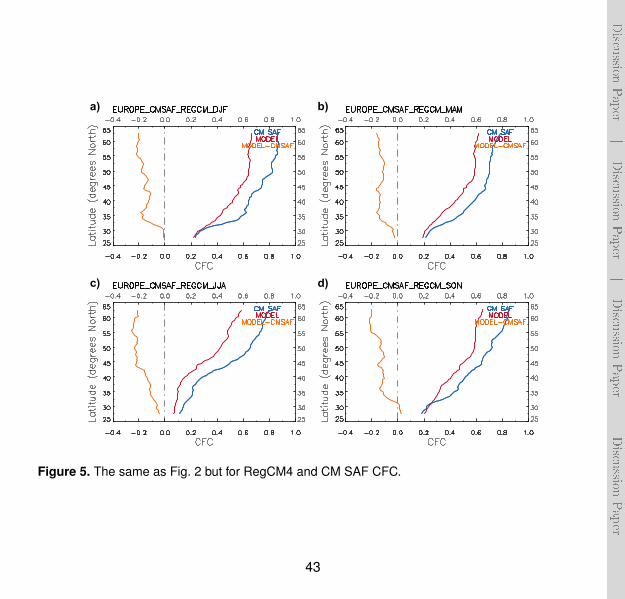
Discu

ssionPaper

|Discu

ssionPaper

|Discu

ssionPaper

|Discu

ssionPaper

|

a) b)

d)c)

Figure 5. The same as Fig. 2 but for RegCM4 and CM SAF CFC.

43

Discu

ssionPaper

|Discu

ssionPaper

|Discu

ssionPaper

|Discu

ssionPaper

|

a) b) c)

d) e) f)

g) h) i)

j)

Figure 6. The same as Fig. 3 but for RegCM4 and CM SAF CFC.

44

Discu

ssionPaper

|Discu

ssionPaper

|Discu

ssionPaper

|Discu

ssionPaper

|

a) b)

c) d)

Figure 7. The same as Fig. 1 but for RegCM4 and CM SAF COT.

45

Discu

ssionPaper

|Discu

ssionPaper

|Discu

ssionPaper

|Discu

ssionPaper

|

a) b)

c) d)

Figure 8. The same as Fig. 2 but for RegCM4 and CM SAF COT.

46

Discu

ssionPaper

|Discu

ssionPaper

|Discu

ssionPaper

|Discu

ssionPaper

|

a) c)b)

e) f)d)

g) h) i)

j)

Figure 9. The same as Fig. 3 but for RegCM4 and CM SAF COT.

47

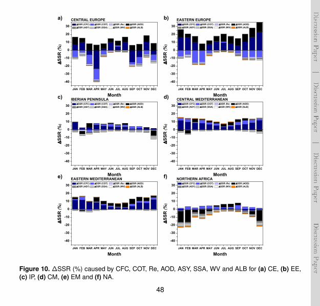
Discu

ssionPaper

|Discu

ssionPaper

|Discu

ssionPaper

|Discu

ssionPaper

|

a) b)

c) d)

e) f)

JAN FEB MAR APR MAY JUN JUL AUG SEP OCT NOV DEC

-40

-30

-20

-10

0

10

20

30

CENTRAL EUROPE SSR (CFC) SSR (COT) SSR (Re) SSR (AOD)

SSR (ASY) SSR (SSA) SSR (WV) SSR (ALB)

S

SR

(%

)

Month

JAN FEB MAR APR MAY JUN JUL AUG SEP OCT NOV DEC

-40

-30

-20

-10

0

10

20

30

EASTERN EUROPE SSR (CFC) SSR (COT) SSR (Re) SSR (AOD)

SSR (ASY) SSR (SSA) SSR (WV) SSR (ALB)

S

SR

(%

)

Month

JAN FEB MAR APR MAY JUN JUL AUG SEP OCT NOV DEC

-40

-30

-20

-10

0

10

20

30

IBERIAN PENINSULA SSR (CFC) SSR (COT) SSR (Re) SSR (AOD)

SSR (ASY) SSR (SSA) SSR (WV) SSR (ALB)

S

SR

(%

)

Month

JAN FEB MAR APR MAY JUN JUL AUG SEP OCT NOV DEC

-40

-30

-20

-10

0

10

20

30

CENTRAL MEDITERRANEAN SSR (CFC) SSR (COT) SSR (Re) SSR (AOD)

SSR (ASY) SSR (SSA) SSR (WV) SSR (ALB)

S

SR

(%

)

Month

JAN FEB MAR APR MAY JUN JUL AUG SEP OCT NOV DEC

-40

-30

-20

-10

0

10

20

30

EASTERN MEDITERRANEAN SSR (CFC) SSR (COT) SSR (Re) SSR (AOD)

SSR (ASY) SSR (SSA) SSR (WV) SSR (ALB)

S

SR

(%

)

Month

JAN FEB MAR APR MAY JUN JUL AUG SEP OCT NOV DEC

-40

-30

-20

-10

0

10

20

30

NORTHERN AFRICA SSR (CFC) SSR (COT) SSR (Re) SSR (AOD)

SSR (ASY) SSR (SSA) SSR (WV) SSR (ALB)

S

SR

(%

)

Month

Figure 10. ∆SSR (%) caused by CFC, COT, Re, AOD, ASY, SSA, WV and ALB for (a) CE, (b) EE,(c) IP, (d) CM, (e) EM and (f) NA.

48