discussion started: 28 may 2018 diurnal variation of ... · manuscript under review for journal...

1

Diurnal variation of aerosol optical depth and PM2.5 in South Korea: a synthesis from AERONET, satellite (GOCI), KORUS-AQ observation, and WRF-Chem model Elizabeth Lennartson1, Jun Wang1,2, Lorena Castro Garcia1, Cui Ge1,2, Greg Carmichael1,2, Meng Gao1,2, Jhoon Kim3, Scott Janz4 5 1Department of Chemical and Biochemical Engineering, University of Iowa, USA

2Center for Global and Regional Environmental Research, University of Iowa, USA 3Department of Atmospheric Science, Yonsei University, S. KOREA 4Lab for Atmospheric Chemistry and Dynamics, Code 614, NASA Goddard Space Flight Center, U.S. A. 10

Correspondence to: Elizabeth Lennartson ([email protected]), Jun Wang ([email protected])

Abstract. Spatial distribution of diurnal variations of aerosol properties in South Korea, both long term and short term, is

studied by using 9 AERONET sites from 1999 to 2017 and an additional 10 sites during the KORUS-AQ field campaign in

May and June of 2016. The extent to which WRF-Chem model and the GOCI satellite retrieval can describe these variations

is also analyzed. In daily average, Aerosol Optical Depth (AOD) at 550 nm is 0.386 and shows a diurnal variation of 20 to -15

30% in inland sites, respectively larger than the counterparts of 0.308 and ± 20% in coastal sites. For all the inland and

coastal sites, AERONET, GOCI, WRF-Chem, and observed PM2.5 data consistently show dual peaks for both AOD and

PM2.5, one at ~ 10 KST and another ~14 KST. In contrast, Angstrom exponent values in all sites are between 1.2 and 1.4

with the exception of the inland rural sites having smaller values near 1.0 during the early morning hours. All inland sites

experience a pronounced increase of Angström Exponent from morning to evening, reflecting overall decrease of particle 20

size in daytime. To statistically obtain the climatology of diurnal variation of AOD, a minimum of requirement of ~2 years

of observation is needed in coastal rural sites, twice more than the urban sites, which suggests that diurnal variation of AOD

in urban setting is more distinct and persistent. While Korean GOCI satellite retrievals are able to consistently capture the

diurnal variation of AOD, WRF-Chem clearly has the deficiency to describe the relatively change of peaks and variations

between the morning and afternoon, suggesting further studies for the diurnal profile of emissions. Furthermore, the ratio 25

between PM2.5 and AOD in WRF-Chem is persistently larger than the observed counterparts by 30-50% in different sites, but

no consistent diurnal variation pattern of this ratio can be found. Overall, the relative small diurnal variation of PM2.5 is in

high contrast with large AOD diurnal variation, which suggests the large diurnal variation of AOD-PM2.5 relationships, and

therefore, the need to use AOD from geostationary satellites for constrain either modeling or analysis of surface PM2.5 for air

quality application. 30

Atmos. Chem. Phys. Discuss., https://doi.org/10.5194/acp-2018-388Manuscript under review for journal Atmos. Chem. Phys.Discussion started: 28 May 2018c© Author(s) 2018. CC BY 4.0 License.

2

1 Introduction

Aerosols, both natural and anthropogenic, play an important role in air quality and the climate. Their presence leads to

pollution events, and they have a direct and indirect role in modifying the Earth’s radiation budget and properties of cloud

and precipitation, respectively (Kaufman et al. 2002). Aerosols also lead to acute and chronic health effects due to their small

size and ability to be inhaled through the respiratory track to the lungs’ alveoli (Pope et al. 2002). As the world continues to 5

industrialize and increase in population (especially in developing countries), it is imperative to understand and mitigate the

effects of pollutants on air quality, climate, and human health, in various spatial and temporal scales.

The United States’ Air Quality Index (AQI) is monitored on a daily basis to inform the population on how clean or

polluted the air in their local area is. The particulate matter (PM) AQI is calculated from “the ratio between 24-hour averages

of the measured dry particulate mass with the National Ambient Air Quality Standard (NAAQS)” (Wang and Christopher 10

2003). For clean conditions, the 24-hour average NAAQS for fine particulate (PM2.5) must be below 35 µg m-3 which is 10

µg m-3 higher than the World Health Organization’s (WHO) recommendation of 25 µg m-3 (EPA 2016; WHO 2006). Due its

health implications and crucial role in determining daily air quality levels, it is of utmost importance to effectively monitor

and predict 24-hour average PM2.5 concentrations.

PM2.5 concentrations are typically measured from surface monitors. In the United States, there are roughly 600 15

continuous (hourly) monitors spread throughout the country and managed by federal, state, local, and tribal agencies (EPA

2008). These monitors provide invaluable information regarding PM2.5 levels in 24 hours per day and are not affected by

clouds since they are fixed at the surface. However, disadvantages include the fact that they do not represent pollution over

large spatial areas. Furthermore, many populated locations in the world do not have a single monitor in their vicinity

(Christopher and Gupta 2010). 20

To gap fill between monitoring sites and provide estimates at locations around the world in emerging need of surface

monitors, recent research has focused on using satellite aerosol optical depth (AOD) to predict ground PM2.5 concentrations.

An early study by Wang and Christopher (2003) relied on a linear relationship to investigate MODIS AOD and 24-hour

average and monthly average PM2.5 concentrations. Other efforts have combined the use of satellite AOD with local scaling

factors from global chemistry transport models, columnar NO2, and factors such as the planetary boundary height, the 25

temperature inversion layer, relative humidity, season, and site location (Liu et al. 2005; Liu et al. 2004; Ma et al. 2016; van

Donkelaar et al. 2010; Zang et al. 2017; Zheng et al. 2016; Qu et al., 2016). A review by Hoff and Christopher (2009)

summarizes that “the satellite precision in measuring AOD is ± 20% and the prediction of PM2.5 concentrations from these

values is ± 30% in the most careful studies.”

Since air quality is often assessed with daily (24 hour) or annual averages of surface PM2.5, while polar-orbiting satellite 30

only provides AOD retrieval once per day for a given location (Wang et al., 2016), recent research has integrated AOD from

geostationary satellites into the surface PM2.5 analysis because a geostationary satellite can provide multiple measurements


3

of AOD per day for a given a location (Wang et al., 2003a; 2003b), thereby better constraining the diurnal variation of PM2.5

for estimating 24-hour average PM2.5 (Xu et al., 2015).

Here, we study the diurnal variation of PM2.5 and AOD and evaluate such variations for air quality applications by

focusing on a six-week long (April – June) air quality campaign in KORUS-AQ and the long-term AERONET sites in South

Korea. The campaign is one of its first kind in east Asia that, through international collaborations, integrated aircraft, surface 5

and satellite data, and air quality models to assess urban, rural, and coastal air quality and its controlling factors. In this

study, we first investigate the long-term AOD diurnal variation for various South Korean ground sites and then focus our

analysis to the KORUS-AQ AOD diurnal variation as described by chemistry transport model and satellite and surface

observations. By centering AOD diurnal variation in our analysis, this study seeks to address the following questions:

1. What is the climatology of AOD diurnal variation in South Korea, both spatially and spectrally? How long should 10

the ground measurement record be needed to derive the climatology of AOD diurnal variation?

2. To that degree can AOD diurnal variation be captured by GOCI (a geostationary satellite) and WRF-Chem (a

chemistry transport model)?

3. What is the diurnal variation of surface PM2.5? How well is the diurnal variation of PM2.5 – AOD relationship

captured by WRF-Chem? 15

The rest of the paper is organized as follows: Section 2 gives a brief overview of previous studies and the motivation for

this research. Section 3 details the datasets used in this study, and Section 4 contains the methods and analysis of the study.

Section 5 closes the paper with a summary and the main conclusions.

2 Background and motivation

2.1 AOD Diurnal Variation 20

The study of AOD diurnal variation dates back to the late 1960s but did not gain momentum until near the turn of the

century (Barteneva et al. 1967; Panchenko et al. 1999; Peterson et al. 1981; Pinker et al. 1994). Peterson et al. (1981) found

the AOD at Raleigh, North Carolina to have an early afternoon maxima at 13-14 local time during the 1969-1975 study

period. Pinker et al. (1994) showed that AOD in sub-Saharan Africa increased throughout the day in December 1987 while

the January 1989 data showed a maxima at 13 local time and minima at 10 and 16 local time. As recent as the early 2000s, 25

the science community agreed that the “diurnal effects are largely unknown and little studied due to the paucity of data…”

(Smirnov et al. 2002).

Most diurnal variation of AOD research stemmed from the analysis of aerosol radiative forcing which requires the

knowledge of the diurnal distribution of key aerosol properties such as AOD, the single scattering albedo, and the asymmetry

factor (Kassianov et al. 2013; Kuang et al. 2015; Wang et al. 2003b). Two early studies developed an algorithm to retrieve 30

AOD diurnal variation from geostationary satellites over water and showed strong AOD diurnal variation during long-range

aerosol transport events; Wang et al. (2003b) used April 2001 hourly data from the GMS5 imager and Wang et al. (2003a)


4

used half-hourly data in July 2000 from the GOES 8 satellites during the ACE-Asia and PRIDE campaigns, respectively.

Consistent with AERONET observations, the GOES 8 retrieval over Puerto Rico showed the dust AOD diurnal variation’s

noontime minimum and early morning or late afternoon maximum. Subsequent work by Wang et al. (2004) investigated the

Taklimakan and Gobi dust regions in China using 1999-2000 AOD data from a nearby airport’s sun photometer. They found

a “season invariant” diurnal change of more than ±10% for dust AOD, with larger values in the late afternoon. Their results 5

aligned with similar past studies which found the diurnal variation of dust aerosols to be ± <5-15% depending on the

AERONET site’s location and distance from a dust source region (Kaufman et al. 2000; Levin et al. 1980; Wang et al.

2003a). However, on a daily basis, the day-to-day variation of AOD can be distinct, up to 150% and both daily diurnal

variation changes and relative departures of AOD from the daily mean are of up to 20% (Kassianov et al. 2013; Kuang et al.

2015). 10

Overall, research based on limited ground-based observations has shown that on a global and annual scale, the AOD

diurnal variation exists, albeit relatively small. On a daily and local scale, AOD diurnal variation is significant which calls

upon the need of geostationary satellite measurements for both air quality and climate studies. Newer geostationary satellites

may play an important role for the future generation of studying AOD diurnal variation.

2.2 PM2.5 Diurnal Variation 15

In addition to AOD diurnal variation, studies have also investigated the diurnal variation of PM2.5. Epidemiological studies

focused on the mass, size, spatial and temporal variability, and chemical composition of PM to investigate the complex

sources and evolution of aerosols in the atmosphere (Fine et al. 2004; Sun et al. 2013; Wittig et al. 2004). In many of these

studies, tracer species of primary aerosols and possible components of secondary organic aerosols were the main focus.

(Edgerton et al. 2006; Querol et al. 2001; Sun et al. 2013; Wittig et al. 2004). 20

Regarding diurnal variation of PM2.5 mass, studies have found different results for various locations around the world.

Querol et al. (2001) used data from June 1999-June 2000 and found Barcelona, Spain’s diurnal variation of PM2.5 in all four

seasons to be characterized by an increase from the late afternoon to midnight. This trend was more pronounced in winter

and autumn since these concentrations were higher than their spring and summertime values.

In the United States, early studies have focused on the Los Angeles, Pittsburgh, and general southeast US areas. Fine et 25

al. (2004) chose two sites, an urban one located at the University of Southern California (USC) and a rural one in Riverside,

and studied the diurnal variation for one week in the summertime and one week in the wintertime. The USC site had a

summer peak in the morning and midday with a winter peak in the morning. The Riverside site experienced a summer peak

in the morning and a winter peak in the overnight hours. The winter results were attributed to the boundary-layer temperature

inversion that forms throughout the day over the area. A few years later in Pittsburgh, Wittig et al. (2004) found no clear 30

PM2.5 diurnal variability due to the combined effect of particulate matter species being transported to the area versus

generated locally. Additionally, they concluded that the daily changes in PM2.5 concentrations could be “attributed to the

major components of the [particulate] mass, namely the sulfate.” Data from the 1998-1999 Southeastern Aerosol and


5

Characterization Study (SEARCH) was used by Edgerton et al. (2006) at four pairs of urban-rural sites. They established the

following three main PM2.5 temporal variation patterns: large values of > 40-50 µgm-3 that occurred on time scales of a few

hours, buildup occurring over several days and then returning to normal levels, and peaks during the summer of similar

magnitude as the monthly or quarterly averages. Their four sites had similar diurnal variations characterized by maxima at 6-

8 a.m. local time and again from 6-9 p.m., similar to those results found by Wang and Christopher (2003) at seven sites in 5

Alabama.

PM2.5 concentrations can significantly vary on relatively short time scales, and in order to understand the potency and

effects of the individual chemical species and PM2.5 as a whole, it is emergently needed to continue to improve the means by

which these measurements are taken, increase the amount of long-term measurements available, and investigate other

methods that can be used to assist with characterizing PM2.5 concentrations and diurnal variation. 10

2.3 Diurnal Variation of AOD-PM2.5 Relationship

Recently, studies have focused on using satellite measurements of AOD in order to predict ground-level PM2.5

concentrations in addition to investigating the diurnal variations of both components. An early study examined how well

MODIS AOD correlated with 24-hour average and monthly average PM2.5 using a linear relationship and found linear

correlation coefficients of 0.7 and 0.9, respectively. Additionally, when the linear relationship used the 24-hour average 15

PM2.5 concentrations, MODIS AOD quantitatively estimated PM2.5 AQI categories with an accuracy of 90% (in terms of

capturing AQI variability) in cloud-free conditions (Wang and Christopher 2003).

Other efforts have used satellite AOD in combination with additional factors to improve the prediction of ground-level

PM2.5, such as the planetary boundary layer height, relative humidity, season, and the geographical characteristics of the

monitoring sites (Liu et al. 2005; Wang et al. 2010). Similarly, Gupta et al. (2006) found a strong dependence on aerosol 20

concentration, relative humidity, fractional cloud cover, and the mixing layer height when analyzing the relationship between

MODIS AOD and ground-level PM2.5. They concluded the importance of local wind patterns for identifying the pollutant

sources and overall, high correlations can occur for the following four conditions: cloud-free, low boundary layer heights,

AOD larger than 0.1 and low relative humidity.

Xu et al. (2015) used GOCI AOD in cloud-free days and a global chemistry transport model (GEOS-Chem) to find 25

significant agreement between the derived PM2.5 and the ground measured PM2.5 for both the annual and monthly averages

over eastern China. Incorporating AOD data from GOCI, a geostationary satellite, provided improvement for GEOS-Chem,

a global chemistry transport model, to estimate ground-level PM2.5 for a highly populated and polluted region of the world

on a fine spatial resolution. When comparing their results to MODIS AOD derived PM2.5, they found better agreement using

their model with an R2 value of 0.66. However, in their study, only daytime-averaged AOD from both GEOS-Chem and 30

GOCI AOD are used as their study concerned about monthly and annual scale.

Hence, one common theme throughout most of the past research, with the exception of Xu et al. (2015), is the use of

AOD data from low-earth orbiting (LEO) satellites to establish the AOD- PM2.5 relationship. However, all the studies have


6

relied on the model-simulated diurnal variation of AOD-PM2.5 relationship to converting satellite-based AOD (often once per

day) to surface PM2.5. An integrated analysis of diurnal variation of AOD, PM2.5, and their relationship, with unprecedented

observations from field campaigns is overdue.

3 Study Area and Data

Over the last 40 years, South Korea has experienced an extensive list of air quality advances for constituents such as lead, 5

sulfur dioxide and PM10 (Ministry_of_Environment 2016). In 2015, they introduced a standard on PM2.5, and due to its recent

implementation, the historical trends of PM2.5 are not well established. Han et al. (2011) suggests that prior to 2005, PM2.5

annual averages either increased or remained constant in rural Chuncheon, South Korea. However, there has been a gradual

decrease in the annual averages in Seoul since 2005, although the decreases have not been continuous (Ahmed et al. 2015;

Ghim et al. 2015; Lee 2014). Annual averages have ranged from 33.5 µg m-3 in 2004 to 21.9 µg m-3 in 2012, but the most 10

recent patterns have been difficult to interpret (Ahmed et al. 2015). Also, since the PM2.5 concentrations discussed above

were from research studies based only in the Seoul region, the aforementioned findings may not be fully applicable to South

Korea as a whole. For this study, we will use all the AERONET data collected over South Korea since early 1990s, as well

as rich data sets collected during KORUS-AQ including additional 10 AERONET sites, GOCI data, and WRF-Chem

modeling data. 15

3.1 AERONET

The AERONET sites provide “long-term, continuous, and readily accessible” aerosol data, with AOD and the Angström

Exponent being two of the available parameters from the direct sun measurements. Sequences are made in eight spectral

bands between 340 nm and 1020 nm while the diffuse sun measurements are made at 440 nm, 670 nm, 870 nm, and 1020 nm

(Holben et al. 1998). The Version 2, Level 2 quality level data are used for this study which implies that the data are cloud-20

screened and quality-assured following the procedures detailed in Smirnov et al. (2000). To compare the AERONET AOD

values to those commonly used by other data platforms such as satellites and models, the AOD at 550 nm is calculated by

using corresponding Angström exponent derived from AOD at 440 nm and 870 nm.

At the time of last access to the AERONET database in July 2017, the stations listed in Table 1 had Version 2, Level 2

data available. These stations were further grouped into the following four land classifications: coastal urban, coastal rural, 25

inland urban, and inland rural. Each site’s classification membership is represented in Figs. 1a and 1b by its marker. The

same marker color schemes are also used in other figures to correspondingly denote AOD diurnal variation at each

individual site.


7

3.2 WRF-Chem

The data from joint Weather Research and Forecasting with Chemistry (WRF-Chem) V3.6.1 model between the University

of Iowa and NCAR is used. WRF-Chem is a regional meteorology-chemistry model capable of simulating both the chemical

and meteorological phenomena within the atmosphere at flexible resolutions to assist with air quality forecasts. It is a fully

coupled “online” model in which both the air quality and meteorological components use the same transport scheme, 5

timestep, grid, and physics schemes for subgrid-scale transport. Additionally, aerosol-radiation-cloud interactions are

considered (Grell et al. 2005).

The University of Iowa’s WRF-Chem forecast for KORUS-AQ provides simulations of meteorology and atmospheric

composition at 20 km and 4 km resolution, respectively. A reduced hydrocarbon chemistry mechanism (REDHC) is added to

expedite computations, and a simplified secondary organic aerosol formation scheme is added to the sophisticated MOSAIC 10

aerosol module. In the vertical, there are 53 layers distributed between the surface and 50 hPa. The bottom layer closest to

the surface has a thickness of ~ 50 m.

To support the KORUS-AQ field campaigns, a Comprehensive Regional Emissions inventory for Atmospheric Transport

Experiments (CREATE) was developed based on GAINS-Asia emissions with updated national data. It has 54 fuel classes,

201 sub-sectors and 13 pollutants, including sulfur dioxide (SO2), nitrogen oxides (NOx), carbon monoxide (CO), non-15

methane volatile organic compounds (NMVOCs), ammonia (NH3), organic carbon (OC), black carbon (BC), PM10, PM2.5,

carbon dioxide (CO2), methane (CH4), nitrous oxide (N2O) and mercury (Hg). The emissions of NMVOCs from vegetation

are calculated online using the MEGAN (Model of Emissions of Gasses and Aerosols from Nature) model, which are

influenced by land use, temperature, and etc. (Guenther et al. 2006). Biomass burning emissions are taken from the GFED

dataset, which is coupled to a plume-rise model (Grell et al. 2011). Sea salt and dust are calculated using Gong et al. (1997) 20

and GOCART (Zhao et al. 2010) schemes, respectively. Chemical initial and boundary conditions are obtained from the

Monitoring atmospheric composition and climate (MACC) global tropospheric chemical composition reanalysis.

WRF-Chem data are retrieved according to the latitude and longitude of each of the 15 AERONET sites that were active

during the KORUS-AQ timeframe (Table 1). Similar to AERONET, the AOD at 550 nm is calculated. The AOD derived in

WRF-Chem is for multiple different observational wavelengths and is based on Angström Exponent relations (Gao et al. 25

2016; Schuster et al. 2006). The WRF-Chem data are available from 01 May 2016 00:00 UTC – 01 May 2016 11:00 UTC

and 02 May 2016 00:00 UTC – 15 June 2016 23:00 UTC.

3.2 GOCI

The Geostationary Ocean Color Imager (GOCI) onboard the Communication, Ocean, and Metrological Satellites (COMS) is

the world’s first geostationary ocean color observation satellite. Launched in 2010, it provides spatial coverage of 2,500 x 30

2,500 km in northeast Asia at a 500-m spatial resolution. The domain is comprised of sixteen image segments (with

resolution of 4 km x 4 km) and the Korean peninsula sits in the center of it. GOCI has six visible and two near-infrared


8

(NIR) bands at 412, 443, 490, 555, 560, and 680 nm and 745 and 865 nm, respectively (Choi et al. 2012). Observations are

taken eight times per day from 00:30 to 07:30 UTC (09:30 to 16:30 KST) (Choi et al. 2017).

To retrieve hourly aerosol data the GOCI Yonsei Aerosol Retrieval (YAER) algorithm was prototyped in 2010 by Lee et

al. (2010) and further developed into its Version 1 (V1) form in 2016 by Choi et al. (2016). The aerosol properties from the

retrieval include AOD at 550 nm, fine-mode fraction at 550 nm, single-scattering albedo at 440 nm, Angström Exponent 5

between 440 and 860 nm, and aerosol type.

Recently, the V1 algorithm has been enhanced to the Version 2 (V2) algorithm and now includes near-real-time (NRT)

processing and improved accuracy in cloud masking, determination of surface reflectance, and selection of surface-

dependent retrieval schemes. The V2 algorithm has shown similar AOD at 550 nm as Moderate Resolution Imagine

Spectroradiometer (MODIS) and Visible Infrared Imaging Radiometer Suite (VIIRS). When validating with AERONET 10

AOD from 2011 to 2016, the V2 reduced median bias and provided an accuracy range of 0.15t + 0.05 compared to V1,

where t is the AERONET AOD value (Choi et al. 2017). For this research, the GOCI YAER V2 AOD at 550 nm data are

downloaded for the KORUS-AQ campaign from 01 May 2016 to 12 June 2016.

3.2 PM2.5

PM2.5 data are downloaded from the KORUS-AQ Data Repository for the entirety of the field campaign. The 10 sites with a 15

corresponding AERONET site nearby are used for this research (Table 2). The three sites of Busan, Gwangju, and Seoul

have multiple sensors within the city limits, thus their total number of observations during the KORUS-AQ timeframe is

much larger than the other seven sites. Additionally, the HUFS site records data every minute while the others take hourly

measurements. All four land classifications are represented within the group, although there is only one inland rural site. All

data during the KORUS-AQ timeframe are downloaded and the number of days with data ranges from 35-41. Overall, there 20

are 51 monitors from Air Korea, six from the National Institute for Environmental Research (NIER), and one was from the

Research Institute on Public Health and Environment (SIHE), and the last was from the Hankuk Institute of Foreign Studies

(HUFS). It should be noted that 51 of the 59 data files had quality control techniques applied to them at the date of last

access in August 2017

4 Methods and analysis 25

4.1 Analysis of AOD Diurnal Variation

The AOD at each hour is computed by using instantaneous AERONET AOD measurements within ± 30 minutes centered

over that hour. The hourly AOD for the same hour in different days is then averaged to compute the climatological (or

baseline) AOD for that hour; the baseline AOD for each hour is then used to compute baseline daily-mean AOD, form which

the diurnal variation of AOD value for each hour can be subsequently calculated. This is completed for the hours of 0-10 30


9

UTC and 21-23 UTC due to the conversion to Korean Standard Time (KST). KST is nine hours ahead of UTC, so the diurnal

variation period extends from 7-18 KST, as the first and last hour are excluded for a lack of observations.

Furthermore, to calculate the statistics for hourly variations, the percent difference from the (baseline) daily mean is

computed. This is referred to as the percent departure from average. Our methods here are similar to the methods from Wang

et al. (2004) and Smirnov et al. (2002). Hence, expressing the departure as a percent allows for comparison to other AOD 5

studies.

The original 22 AERONET sites are split into four land classifications to further analyze and define trends amongst their

AOD diurnal variations at 550 nm. The sites of Chinhae, Korea University, and Kyungil Univsersity are excluded from the

analysis due to the short data records, leaving 19 AERONET sites. Each site’s full record of data is used in the calculation

(Table 1). Figure 1 shows a summary of this classification. Of the 19 sites, three are coastal urban, five are coastal rural, six 10

are inland urban, and five are inland rural.

Shown in Fig. 2 is the AOD diurnal variation and percent departure from daily mean using the full record of data at all 19

AERONET sites, split into land classification. The coastal rural sites show the most similarity amongst each other and are

characterized by AOD levels remaining virtually constant throughout the day as their departure from the daily mean is

generally ± 10%. This feature agrees with Smirnov et al. (2002) who also found that the Anmyon site, on the western coast 15

of the Korean peninsula, has little to no diurnal variation of AOD at 500 nm when investigating a multiyear data record.

The AOD diurnal variation of the coastal urban sites is more pronounced with a departure from the daily average at ±

20% and has fewer similarities between sites versus the coastal rural classification. The KORUS NIER site has noticeably

higher values of AOD than the Gangneung or Pusan for the majority of the day until 18 KST. These sites are urban in nature

and therefore have their own emissions characteristics, adding an additional layer of complexity to their distinctive diurnal 20

variations. This could explain why the coastal urban sites experience more variation than the coastal rural sites. When

focusing on the different diurnal variations amongst the coastal urban sites, we believe that the differences could stem from

the site location. For example, the sites on the western Korean peninsula (i.e., KORUS NIER) are closer to Chinese

emissions and may be impacted more by long-range transport than the coastal urban sites on the eastern Korean peninsula

(i.e., Pusan and Gangneung). When combined with local emissions, the external factors could lead to a different diurnal 25

variation than their counterparts on the eastern side of the country.

All six of the inland urban sites show remarkably similar diurnal variations. Their AODs slightly decrease and remain

constant until the early afternoon at approximately 14 KST when the AOD then gradually builds until 18 KST. One outlier to

this evening-build characteristic is KORUS Olympic Park whose AOD values drop between 17 and 18 KST. As a whole,

their average departure from the daily mean is ±20% with the most negative values occurring in the midday (i.e, the inland 30

urban sites experience a minima in AOD values during this time). The early morning and late evening increases could be

attributed to an increase in traffic and transportation demands. It is interesting to note that this common diurnal variation

trend is seen at sites that have as little as four months of data (i.e., KORUS Iksan) to greater than five years of data (i.e.,


10

Gwangju and Yonsei University). Below in section 4.3, we investigate this further to quantify how long of a record is needed

at each site to match the diurnal variation produced by the full record.

The five inland rural sites naturally divide into two groups. KORUS Daegwallyeong, located on the eastern part of the

peninsula, shows a much lower magnitude of AOD around 0.2-0.3 throughout the entire day. The other four locations of

Hankuk, KORUS Baeksa, KORUS Songchon, and KORUS Taehwa have higher AOD values near 0.4-0.6 in the morning 5

before decreasing throughout the day and eventually rising again in the early evening at 15-16 KST. The only two exceptions

to this trend are Hankuk and KORUS Songchon, located east-south-east of Seoul, that experience slight noontime increases.

After the early evening build-up, most of the sites’ AOD decreases at 17-18 KST, again with the exception of Hankuk and

KORUS Songchon. The inland rural sites have the most variation for their percent departure from average with some sites

such as KORUS Baeksa and KORUS Songchon approaching -30% at 12 KST and 15 KST, respectively, and KORUS 10

Daegwallyeong staying between ±10% with the except of 16 and 17 KST.

Overall, we see similar trends for the coastal sites and for the inland sites. The coastal urban and coastal rural sites have a

lower average AOD value of 0.308 compared to the inland urban and inland rural sites whose average AOD value is 0.386.

Additionally, regardless of land classification, most sites see an early morning and late afternoon maxima AOD and

noontime minima AOD. Factors influencing the diurnal variation include length of data record, number of available 15

measurements for calculating the hourly averages, and site location compared to those sharing its land classification.

4.2 Analysis of Angström Exponent Diurnal Variation

Similar to the AOD diurnal variation, each site’s full record of data is used to compute diurnal variation of the Angström

Exponent. The same analysis procedure is used, but instead of calculating AOD at 550 nm, the only variable of interest is the

Angström Exponent between 440 nm and 675 nm. The Angström Exponent is of importance since it helps determine the 20

aerosol’s source. It is inversely related to the average size of aerosol particles, so the smaller the particles, the larger the

value. Generally speaking, an Angström Exponent approaching 0 signifies coarse-mode or larger particles such as dust, and

an Angström Exponent greater than or approaching 2 signifies fine-mode or smaller particles such as smoke from biomass

burning (Wang et al. 2004). The size of the particle assists with attributing the aerosol to natural or anthropogenic sources

since the latter are typically smaller than their natural counterparts (of dust and sea salt particles). 25

All four land classifications show similar Angström Exponent values in the range of 1.2-1.6 with the exception of lower

values near 1.0 at the inland rural sites (Fig. 3). All six of the inland urban sites experience a gradual build in Angström

Exponent from 1.2 to 1.4 throughout the day. The coastal urban sites are similar, as Pusan and Gangneung also see an

increase in Angström Exponent, but the KORUS NIER site has a noticeable Angström Exponent maxima near 1.2 at 10

KST. Also, its values are lower than the other coastal urban or inland urban sites, with a range of 1.1 to 1.2. However, the 30

general trend of the coastal urban sites is that they too gradually increase in Angström Exponent as the day progresses.

Turning to the rural sites, all five of the inland rural sites experience the same gradual build throughout the day to 1.4 as

the inland urban sites, but their values start a bit lower near 1.0 versus 1.2. The coastal rural sites hover ~1.3 for the majority


11

of the day, with KORUS UNIST Ulsan experiencing values as high as 1.5 from 12-16 KST before dropping back down to

1.4 by 17 KST. The Angström Exponent diurnal variation of the coastal rural sites is not as pronounced as that in the other

three land classifications that all experience morning Angström Exponent minimums and gradually build throughout the day

before plateauing.

With the typical range of 1.2-1.6 experienced at most sites, it is concluded that the majority of aerosols over the Korean 5

peninsula are fine-mode particles with some coarser-mode particles seen overnight and in the early morning. As the day

progresses, the particle size decreases due to secondary organic aerosol formation which leads to an increase in the

Angström Exponent.

4.3 Observation Time for Climatologically-representative AOD Diurnal Variation

In this section, we define the term “climatological diurnal variation”. This is the diurnal variation pattern produced at each 10

AERONET site in long term averages such that it is relatively persistent and statically robust. The concept is similar to the

concept of climatology of diurnal variation of 2-m air temperature which, while varying with location, normally shows peak

in the afternoon and minimum before the Sun rise [Wang and Christopher, 2006]. The concept of “climatological diurnal

variation of AOD or aerosol properties”, therefore builds upon the hypothesis that there are underlying processes inherent

with respect to a specific location to produce diurnal variation of AOD. For example, in the agricultural burning seasons over 15

Central America, AOD values often peak around later afternoon and are minimal in the night before Sun rises; this is

because such burnings often started in the late morning and diminishes at night [Wang et al., 2006]. Hence, an intriguing

question is that how long our data record should be to obtain climatological diurnal variation of AOD or aerosol properties.

We address this question by data collected at the five AERONET sites which have more than five years of data in their full

record: Anmyon, Baengnyeong, Gosan, Gwangju, and Yonsei University. 20

To statistically compare how long of a data record is needed to match the climatological diurnal variation, we first

compute the statistics starting from the first month of the data record to a certain number of months, n; hereafter the subset of

the data is denoted as [1, n], with the first number being the starting of the month, and second number the last month in the

subset. We then repeat the calculation by moving the starting month (and ending month) with increment of one month each

time, e.g., for the data subset [2, n+1], [3, n+2], …, [N-n+1, N], where N is the total number of months of whole data record. 25

The average of diurnal variation statistics from each n-month data subset is then compared with statistics of diurnal variation

from the whole data record. The comparison reveals the degree to which n month data record may describe the

climatological diurnal variation derived from full data record for a specific site of interest. We then repeat the same process

by increasing the number of months for the subset (n) by one month, two months, three months, …, until the subset

eventually grows to the full record. It is expected that as n increases, the climatological diurnal variation will be better 30

characterized.


12

The actual implementation of the method above requires the removal of the gaps of missing data, e.g., months that don’t

have observation. Hence, Anmyon, Baengnyeong, Gosan, Gwangju, and Yonsei University are left with full records of 89,

53, 80, 82, and 71 months, respectively, for the analysis.

Figure 4 shows that as n, the number of months of observation increases, the diurnal variation being described by these

subset observation is in more agreement with the counterpart from the full record, in terms of linear correlation coefficient R, 5

root mean square error (RMSE), and statistical significance. The inland urban sites of Gwangju and Yonsei University have

very similar results (Figs. 4d and 4e). Gwangju requires 13 months of data to become significant (p < 0.05), or roughly

15.9% of the full (82 months) record of data. Yonsei requires 11 months of data which is slightly lower at 15.5% (of 71

months). Additionally, they both have a R-value around 0.8 at the occurrence of the first significance, and their results

become significant shortly after the RMSE and R-value graphs intersect. We conclude that the inland urban sites require 10-10

12 months of data to match the climatological diurnal variation with an R value of 0.8 and p < 0.05. Additionally, they

require 45-47 months of data for an RMSE < 0.02.

The results for coastal rural sites of Anmyon, Baengnyong, and Gosan are less c (Fig. 4 a-c). They require more data than

the urban sites before becoming significant (p < 0.05) with a range from 18% to 32%. Anmyon requires 18% of the total data

with 16/89 months and Baengnyeong and Gosan require about 30% of the total data with 17/53 and 24/80 months, 15

respectively. They have slightly lower R-values of 0.57-0.78 at the time of their first significance, and similar to the inland

urban sites, their correlations become significant after the intersection of the RMSE and R-value graphs. These three sites

require 21-25 months of data to match their climatological diurnal variations with an R value of 0.8 and p < 0.05, which is

twice of that of the inland urban sites. Overall, RMSE < 0.02 can be reached with 35-52 months of data in the subset; this is

similar to the inland urban sites, but a much greater range. The varied location of these three coastal rural sites could explain 20

the variability between them, as they extend from Baengnyeong near North Korea to Gosan off the southern coast of the

Korean peninsula.

Between the five sites that we investigated, there is no consistent pattern among the number of months of full record data

required for diurnal variation replicability and significance. Baengnyeong, the site with the least amount of full record data

(53 months), requires 16 months (32%) of the data, while Yonsei (71 months of data) requires 11 months (15.5%), Gosan 24 25

months, Gwangju 13 month, Anmyon 16 months. In average, ~18 months of observation data are needed to obtain

statistically significant results for characterizing the diurnal variation of AOD.

One findings surprising but interesting to note is that coastal rural sites would require twice longer observation than the

inland urban sites to match the climatological diurnal variation with R = 0.8 and p < 0.05. We thought that due to the

complexity of the urban sites having both their own emissions and those via background and transport, they would require 30

more data for a common trend to emerge. However, it is in fact just the opposite, suggesting that diurnal variation of AOD in

urban setting is distinct and persistent.


13

4.4 Analysis of WRF-Chem and GOCI AOD

The WRF-Chem model provided hourly chemical weather forecasts from 1 May 2016 to 15 June 2016. Thus, this is defined

as the KORUS-AQ timeframe, and spatial and temporally matched data pairs between GOCI-AEROENT and WRF-Chem

AERONET are analyzed. Because of clouds, GOCI AOD data is rarely eight time per day, while the AERONET data also

undergoes its own quality control algorithms. In contrast, the WRF-Chem data is available for every hour during the 5

timeframe of interest. Due to these factors, the intercomparision dataset is the smallest between AERONET vs GOCI (1,583

data pairs) and the largest between AERONET vs WRF-Chem (3,633 data pairs).

The scatter plots between observation (x-axis) and either model or GOCI (y-axis) is shown in Fig. 5, while the color of

each scatter plot point represents the density of observations within that data range. Although both are statistically significant

(p < 0.001), the AERONET vs GOCI R-value of 0.8 is double that of the AERONET vs WRF-Chem R-value of 0.4. 10

Additionally, the RMSE value between AERONET vs GOCI is lower as well. Overall, WRF-Chem can both over- and

under-predicted the AERONET AOD values while the GOCI satellite typically underpredicted them during the KORUS-AQ

timeframe. In reference of the AERONET AOD values, GOCI AOD is better than WRF-Chem predictions.

To analyze these results on a site basis, Taylor Diagrams are produced (Fig. 6), in which the radius represents the

normalized standard deviation while the correlation coefficient is represented as cosine of polar angle. Hence, regardless of 15

the data sources, the observation data will be represented at the one point (with normalized standard deviation of 1 and

cosine of polar angle of 1). The color of data points shows the data bias with respect to the observation.

Figure 6a shows that WRF-Chem both over- and under-predicted AOD values during the campaign, and there is no clear

indication whether the WRF-Chem performed consistently better for certain land classification (within 15 sites we analyzed).

For example, looking at the inland urban sites, WRF-Chem underpredicted two sites (KORUS Olympic Park and KORUS 20

Iksan), overpredicted two sites (Gwangju and KORUS Kyungpook), and had no bias at one site (Yonsei University). The R

values range from 0.15 to 0.7 with the majority of points between 0.15 and 0.4. Lastly, there is an even distribution of sites

where the WRF-Chem standard deviation is higher than and less than the AERONET standard deviation.

Figure 6b shows the relationship between AERONET and GOCI at the same 15 sites during the KORUS-AQ campaign.

Here, we see that only three sites (Baengnyeong, KORUS NIER, and KORUS Daegwallyeong) had a positive bias and thus 25

were over predicted by GOCI. Noticeably different from 6a is the shifted R value range, now extending from 0.35 to 0.9 but

concentrated within 0.7 to 0.9. Another interesting difference is that the GOCI standard deviation was greater than the

AERONET standard deviation at all 15 sites, suggesting COCI AOD tends to amply the temporal variation of AOD.

4.5 PM2.5 Diurnal Variation

Table 2 lists information for all PM2.5 sites, including their full record of data, the number of recorded observations within 30

that full record, the nearby AERONET station, the number of days having data recorded, and the hours of minima and

maxima PM2.5. Nine of the ten sites reported data in hourly averages. For the HUFS site whose data was reported minutely,


14

the hourly averages are created by computing the mean of data in that hour, as is done by most analysis of hourly PM2.5.

Again, only 7-18 KST is analyzed for PM2.5.

As seen in Fig. 7, the PM2.5 diurnal variations are surprisingly invariant given the short timeframe of interest. One would

expect that as the data timeframe decreases, the fluctuations would increase. However, this is not the case for PM2.5. The

coastal urban sites of Busan and Bulkwang remain near 30-35 µg m-3 throughout the day (Fig. 7a). Bulkwang does slightly 5

increase at 8 KST but then returns to the constant value of 30 µg m-3 by 11 KST. The inland urban sites (Fig. 7b) closely

resemble the coastal urban sites in diurnal pattern and value except for Olympic Park. Its values were double the other inland

and coastal urban sites at 60 µg m-3 at its 8 KST maximum. Concentrations then drop to near 45 µg m-3 for 13-18 KST.

Olympic Park shows the most fluctuations throughout the day in its PM2.5 concentrations.

The coastal rural sites (Fig. 7c) of Jeju, Baengnyeong, and KORUS UNIST Ulsan split into three diurnal variations that 10

are varied in concentration and each with its own unique pattern. The KORUS UNIST Ulsan site has the highest

concentrations near 30 µg m-3 but exhibits little to no fluctuations throughout the day. The Baengnyeong site has the second

highest concentrations near 25 µg m-3 with a 14 KST maximum. Jeju has the lowest concentrations near 15 µg m-3 and

maxima at 11 and 14 KST with a 10 and 13 KST minima. HUFS, the inland rural site (Fig. 7d), fluctuates between its 8 KST

maxima near 40 µg m-3 and drops to a concentration near 30 µg m-3 by 12 KST and remains there for the rest of the day. 15

Overall, seven of the ten sites have stagnant PM2.5 values near 30 µg m-3 throughout the entire day. The other three sites,

Bulkwang, Daejeon, and HUFS all have morning PM2.5 maxima at 8 KST before dropping to stagnant values by 13 KST.

Daejeon experiences abnormally highest PM2.5 concentrations with values peaking near 60 µg m-3. For all sites, the

correlation between hourly PM2.5 variation and daily-mean PM2.5 variation (Fig. 8) has the highest R2 value above 0.8 at

noontime, and decreases toward early morning and later afternoon, reaches the minimum at mid-night, which suggests that 20

day-time variation of emission and boundary layer process are dominant factors affecting day-to-day variability of PM2.5.

4.6 AOD-PM2.5 Diurnal Variation Relationship

Here we study which data source (from GOCI or WRF-Chem) either predicted or retrieved the AERONET AOD values

better. We also compare the AOD diurnal variation to the PM2.5 diurnal variation. In Fig. 9, the diurnal variations are shown

for AERONET, WRF-Chem, GOCI, observed PM2.5, and WRF-Chem predicted PM2.5 for the sites that have all five dataset 25

available (ie: the sites listed in Table 2). All data is temporally and spatially matched. Due to its retrieval times, GOCI’s

AOD diurnal variation only extends from 9-16 KST, thus only 9-16 KST is used for AERONET and WRF-Chem as well.

The GOCI AOD values better matched the observed AERONET AOD diurnal variation. As seen in Fig. 9a, although

hourly GOCI AOD has a systematic low bias of 0.02-0.05 with respect to the AEROENT counterparts, the GOCI AOD

diurnal variation (green line) mirrors that of AERONET (blue line) for the entire day, showing low values around noon and 30

dual peaks (one in 10-11 KST) in the morning and (another 14 KST) in the afternoon, respectively; both GOCI and

AERONET also shows that the minimum AOD is in the later afternoon at 16 KST, although GOCI shows a relatively larger


15

decrease of AOD from 14 KST to 16 KST. In contrast, while WRF-Chem AOD values are consistent with GOCI and

AOERNET to describe the dual peaks and low AOD values around noon, a much stronger peak at 16 KST (than that at 10

KST) in WRF-Chem differs that from GOCI and AEROENT (both of which show comparable dual peaks). Furthermore,

WRF-Chem shows a relatively increase of (minimum) AOD at 9 KST to 15 and 16 KST, while GOCI and AEROENT both

show the decrease with minimum AOD at 16 KST. Hence, it is hypothesized that the diurnal emission in WRF-Chem may 5

have too much skewness toward afternoon emission; indeed WRF-Chem AOD is comparable to AERONET AOD values in

the morning, but shows large positive bias up to 0.08 in the later afternoon. This hypothesis needs to be further studied.

Also plotted in Fig. 9a is the average observed and WRF-Chem predicted PM2.5 diurnal variation of the 10 PM2.5 sites.

The observed concentrations peak at 10 KST with a value approaching 33 µg m-3 but drop to less than 28 µg m-3 by 13 KST,

and then peak again to 30 µg m-3 at 14 KST. WRF-Chem predicted PM2.5 is systematically higher than observed PM2.5 by 10

10-15 µg m-3, but it has similar dual peaks at 10 and 14 KST. Similar as its AOD variables, WRF Chem showed that the

peak at 14 KST is ~3 µg m-3 higher than the peak at 10 KST, while observed PM2.5 show that the peak at 14 KST is ~5 µg m-

3 lower than the peak at 10 KST. Furthermore, WRF-Chem shows an increase of PM2.5 from 11 to 13 KST while the

observed PM2.5 showed the opposite. Overall, the observed PM2.5 concentrations decrease from morning (9-10 KST) to

evening (15-16 KST), but WRF-Chem counterparts show the opposite. Hence, the comparison and contrast analyses of both 15

AOD and PM2.5 suggest further studies for the diurnal variation of emission in WRF-Chem.

In general, the diurnal variation of AERONET AOD (averaged over all sites) fluctuates the least throughout the day with

a percent departure from the daily mean of ± 6%. WRF-Chem fluctuates ± 8% while GOCI shows the most variation at +9%

to -30% due to an outlying low value at 16 KST. Similar to AERONET and WRF-Chem, the PM2.5 percent departure from

daily mean ranges from ± 8%. 20

Figure 9b displays the diurnal variation of the PM2.5/AOD ratio derived from WRF-Chem and collocated AERONET and

PM2.5 measurement throughout the KORUS-AQ campaign. This ratio is valuable because satellite AOD often is used to

multiply this ratio to derive surface PM2.5. While the ratio from WRF-Chem overall is larger than observation-based

counterparts by 30-50% in all sites (except Daejeon for some hours and one outliner at a particular hour in Gwangju site), the

majority of the ratios range from 60-140 µg m-3 t-1 with outliers as low as 40 and as high as 160 µg m-3 t-1. Overall, there is 25

no apparent trend between PM2.5/AOD ratio and time of day. This conclusion is consistent even when analyzing based on

land classification. The three coastal rural sites of Baengnyeong, Jeju, and Ulsan have ratio maximums in both the morning

(7, 8, and 10 KST) and early evening (17 KST). Their minimums range from morning (9 KST), noontime, and late afternoon

(16 KST). The two coastal urban sites of Bulkwang and Busan show more similarities with peaks in the early morning (8 and

9 KST) but still have a minimum range from noontime to afternoon (12 and 15 KST). The inland urban sites have morning 30

(9 and 10 KST), afternoon (13 KST), and early evening (17 and 18 KST) maximums but cohesively have a 15 KST minima,

aside from Gwangju whose ratio steadily increases after 10 KST. Being the only inland rural site, the PM2.5/AOD at HUFS


16

has a maxima at 8 KST and steadily decreases afterward for the remainder of the day. This conclusion suggests that diurnal

variation is not a prominent factor in using the PM2.5/AOD ratio to derive PM2.5 values from AOD.

4 Summary and conclusions

By using all possible AEROENET data in South Korea, the surface observation of PM2.5, GOCI AOD and WRF-Chem

simulated AOD during KORUS-AQ Field Campaign in South Korea from April to June 2016, this study analyzed the 5

diurnal variation of aerosol properties and surface PM2.5 from surface observations, and assessed their counterparts from

models. In summary, the following were found.

1. Long-term AEROENT data shows that the climatological AOD diurnal variation is very similar amongst South

Korean AERONET sites. Most see an AOD maxima in the middle morning (10 am) and middle afternoon (2 pm)

and a noontime AOD minima. Additionally, the coastal sites have lower average values near 0.3 at 550 nm while the 10

inland sites have higher values near 0.4. The inland sites also experience the most AOD fluctuations during the day

on the order of +20% to -30%. Analysis of the Angström Exponent shows a gradual increase throughout the day

from 1.2 to 1.4.

2. Given there is a persistent diurnal variation of AOD and Angstrom Exponent in South Korea, we analyzed that at

minimum, there should be more than 12 months of observation, and the coastal rural sites require twice of 15

observations than the inland urban sites, to characterize the climatology of diurnal variation of AOD at statistically

significant level. This suggests the distinct and persistent diurnal variation of aerosol properties in urban areas.

3. The AERONET and GOCI AOD had a linear correlation coefficient of (R) 0.8 and RMSE = 0.16 while the

AERONET and WRF-Chem relationship had R = 0.4 and RMSE = 0.28, suggesting that AOD data retrieved from

GOCI satellite shows a closer agreement with AERONET AOD data than those from WRF-Chem model. 20

4. Analysis of 10 AERONET-surface PM2.5 paired sites show that the diurnal variation of PM2.5 was ~10% throughout

the day, with the exception of the Daejeon and HUFS sites having a maxima at 8 KST (or peaks by 20%) and values

gradually decreasing and remaining steady for the remainder of the day after 12 KST. PM2.5 daily-mean values were

around 30 µg m-3 which is still 20 µg m-3 below the 24-hour PM2.5 air quality standard in South Korea but 5 µg m-3

above the WHO recommendation. Overall, the day-to-day variation of mean PM2.5 at all sites can be best described 25

by the variation of hourly PM2.5 data at noontime for each day, and is least captured by the variation of PM2.5 in the

mid-night hours.

5. AERONET, GOCI, WRF-Chem, and observed PM2.5 data consistently show dual peaks for both AOD and PM2.5,

one at 10 KST and another that 14 KST. However, WRF-Chem show the peak in afternoon is larger than the peak in

the morning, which is opposite from what GOCI and AERONET reveal. Consequently, WRF-Chem shows increase 30

of AOD and PM2.5 from 9 KST to 16 KST, which contrasts with the deceasing counterparts in GOCI, AEROENT,


17

and observed PM2.5. The analysis suggests that the diurnal profile of emissions in WRF-Chem may have a too larger

skewness toward the afternoon.

6. PM2.5/AOD ratio ranged from 60-120 throughout the day, and no consistent pattern was seen at the 10 sites nor when

further broken down into land classification. The ratio in WRF-Chem is persistently larger than the observed

counterparts by 30-50% in different sites. This highlights the combined need to use satellite to characterize aerosol 5

2D information and use chemistry transport models to resolve the space of vertical prolife toward improved estimate

of surface PM2.5.

By using rich data sets during KORUS-AQ, this study revealed there are persistent diurnal variation of AOD and

surface PM2.5 in South Korea. It is shown that the Korean GOCI satellite is able to consistently capture the diurnal

variation of AOD, while WRF-Chem clearly has the deficiency to describe the relatively change in the morning and 10

afternoon. As a minimum of one-year observation is required to fully characterize the climatology of diurnal variation

pattern of AOD, future field campaigns are commended to have at least longer time periods of surface observations

where AEROENT and surface PM2.5 network can be collocated. Hence, future studies are needed to evaluate the

statistical significance of our analysis of diurnal variation of PM2.5/AOD ratios with a longer record of observation data.

Acknowledgement 15

This research is in part supported by NASA’s GEO-CAPE program and in part by KORUS-AQ program (grant #:

NNX16AT82G). AERONET data are downloaded from http://aeronet.gsfc. nasa.gov and we thank all AERONET PIs in

South Korea for collecting the data.

References

Aman, A. A. and Bman, B. B.: The test article, J. Sci. Res., 12, 135–147, doi:10.1234/56789, 2015. 20

Aman, A. A., Cman, C., and Bman, B. B.: More test articles, J. Adv. Res., 35, 13–28, doi:10.2345/67890, 2014.

Ahmed, E., K. H. Kim, Z. H. Shon, and S. K. Song.: Long-term trend of airborne particulate matter in Seoul, Korea from

2004 to 2013. Atmos. Environ., 101, 125-133, 2015.

Al-Saadi, J., G. Carmichael, J. Crawford, L. Emmons, and S. Kim.: White Paper: NASA Contributions to KORUS-AQ: An

International Cooperative Air Quality Field Study in Korea, 2015. 25

Barteneva, O.D., Y.N. Dovgyallo, and Y.A. Polyakova.: Investigations of the optical properties of the atmospheric surface

layer. Proc. Main Geophys. Obs. (Trudy GGO) (in Russian), 36, 119-140, 1967.

Center for Global and Environmental Research (CGRER).: KORUS-AQ. Accessed 29 August 2017,

https://cgrer.uiowa.edu/korus-aq, 2010.


18

Choi, J. K., Y. J. Park, J. H. Ahn, H. S. Lim, J. Eom, and J. H. Ryu.: GOCI, the world's first geostationary ocean color

observation satellite, for the monitoring of temporal variability in coastal water turbidity. J. Geophys. Res.-Oceans, 117, 10.

Choi, M., and Coauthors, 2016: GOCI Yonsei Aerosol Retrieval (YAER) algorithm and validation during the DRAGON-NE

Asia 2012 campaign. Atmos. Meas. Tech., 9, 1377-1398, 2012.

Choi, M., J. Kim, J. Lee, M. Kim, Y. Park, B. Holben, T. Eck, Z. Li, C. Song.: GOCI Yonsei aerosol retrieval version 2 5

aerosol products: improved algorithm description and error analysis with uncertainty estimation from 5-year validation over

East Asia. Atmos. Meas. Tech., https://doi.org/10.5194/amt_2017_251, 2017.

Christopher, S. A., and P. Gupta.: Satellite remote sensing of particulate matter air quality: the cloud-cover problem. J. Air

Waste Manage. Assoc., 60, 596-602, 2010.

Edgerton, E. S., B. E. Hartsell, R. D. Saylor, J. J. Jansen, D. A. Hansen, and G. M. Hidy.: The southeastern aerosol research 10

and characterization study, part 3: continuous measurements of fine particulate matter mass and composition. J. Air Waste

Manage. Assoc., 56, 1325-1341, 2006.

EPA.: Ambient Air Monitoring Strategy for State, Local, and Tribal Air Agencies AAMS for SLTs, 95 pp, 2008.

EPA.: NAAQS table. [Available online at https://www.epa.gov/criteria-air-pollutants/naaqs-table.], 2016

Fine, P. M., B. Chakrabarti, M. Krudysz, J. J. Schauer, and C. Sioutas.: Diurnal variations of individual organic compound 15

constituents of ultrafine and accumulation mode particulate matter in the Los Angeles basin. Environ. Sci. Technol., 38,

1296-1304, 2004.

Gao, M., and Coauthors.: Modeling study of the 2010 regional haze event in the North China Plain. Atmos. Chem. Phys., 16,

1673-1691, 2016.

Ghim, Y. S., Y. S. Chang, and K. Jung.: Temporal and spatial variations in fine and coarse particles in Seoul, Korea. Aerosol 20

Air Qual. Res., 15, 842-852, 2015.

Gong, S.L, L.A Barrie, and J.P. Blanchet: Modeling sea-salt aersols in the atmosphere .1. model development. J. Geophys.

Res.: Atmos., 102, 3805-3818, 1997.

Grell, G. A., S. E. Peckham, R. Schmitz, S. A. McKeen, G. Frost, W. C. Skamarock, and B. Eder: Fully coupled "online"

chemistry within the WRF model. Atmos. Environ., 39, 6957-6975, 2005. 25

Grell, G.A., S.R. Freitas, M. Stuefer, and J. Fast.: Inclusion of biomass burning in WRF-Chem: impact of wildfires on

weather forecasts. Atmos. Chem. Phys., 11, 5289-5303, 2011.

Guenther, A., T. Karl, P. Harley, C. Wiedinmyer, P.I. Palmer, and C. Geron.: Eastimate of global terrestiral isoprene

emissions using MEGAN (model of emissions of gases and aerosols from nature). Atmos. Chem. Phys., 6, 3181-3210, 2006.

Gupta, P., S. A. Christopher, J. Wang, R. Gehrig, Y. Lee, and N. Kumar.: Satellite remote sensing of particulate matter and 30

air quality assessment over global cities. Atmos. Environ., 40, 5880-5892, 2006.

Han, Y. J., S. R. Kim, and J. H. Jung.: Long-term measurements of atmospheric PM2.5 and its chemical composition in rural

Korea. J. Atmos. Chem., 68, 281-298, 2011.


19

Hoff, R. M., and S. A. Christopher.: Remote sensing of particulate pollution from space: have we reached the promised land?

J. Air Waste Manage. Assoc., 59, 645-675, 2009.

Holben, B. N., and Coauthors.: AERONET - A federated instrument network and data archive for aerosol characterization.

Remote Sens. Environ., 66, 1-16, 1998.

Kassianov, E., J. Barnard, M. Pekour, L. K. Berg, J. Michalsky, K. Lantz, and G. Hodges.: Do diurnal aerosol changes affect 5

daily average radiative forcing? Geophys. Res. Lett., 40, 3265-3269, 2013.

Kaufman, Y. J., D. Tanre, and O. Boucher, 2002: A satellite view of aerosols in the climate system. Nature, 419, 215-223.

Kaufman, Y. J., B. N. Holben, D. Tanre, I. Slutsker, A. Smirnov, and T. F. Eck: Will aerosol measurements from Terra and

Aqua polar orbiting satellites represent the daily aerosol abundance and properties? Geophys. Res. Lett., 27, 3861-3864,

2000. 10

Kuang, Y., C. S. Zhao, J. C. Tao, and N. Ma.: Diurnal variations of aerosol optical properties in the North China Plain and

their influences on the estimates of direct aerosol radiative effect. Atmos. Chem. Phys., 15, 5761-5772, 2015.

Lee, J., J. Kim, C. H. Song, J. H. Ryu, Y. H. Ahn, and C. K. Song.: Algorithm for retrieval of aerosol optical properties over

the ocean from the Geostationary Ocean Color Imager. Remote Sens. Environ., 114, 1077-1088, 2010.

Lee, M.: An analysis on the concentration characteristics of PM2.5 in Seoul, Korea from 2005 to 2012. Asia-Pac. J. Atmos. 15

Sci., 50, 33-42, 2014.

Levin, Z., J. H. Joseph, and Y. Mekler.: Properties of sharav (khamsin) dust – comparision of optical and direct sampling

data. J. Atmos. Sci., 37, 882-891, 1980.

Liu, Y., J. A. Sarnat, A. Kilaru, D. J. Jacob, and P. Koutrakis.: Estimating ground-level PM2.5 in the eastern united states

using satellite remote sensing. Environ. Sci. Technol., 39, 3269-3278, 2005. 20

Liu, Y., R. J. Park, D. J. Jacob, Q. B. Li, V. Kilaru, and J. A. Sarnat.: Mapping annual mean ground-level PM2.5

concentrations using Multiangle Imaging Spectroradiometer aerosol optical thickness over the contiguous United States. J.

Geophys. Res.: Atmos., 109, 10, 2004.

Ma, Z. W., Y. Liu, Q. Y. Zhao, M. M. Liu, Y. C. Zhou, and J. Bi.: Satellite-derived high resolution PM2.5 concentrations in

Yangtze River Delta Region of China using improved linear mixed effects model. Atmos. Environ., 133, 156-164, 2016. 25

Ministry of Environment: Air quality standards and air pollution level. [Available online at

http://eng.me.go.kr/eng/web/index.do?menuId=252.]

Panchenko, M.V., Yu. A. Pkhalagov, R.F. Rakhimov, S.M. Sakerin, and B.D. Belan.: Geophysical factors of the aerosol

weather formation in Western Siberia. Optica atmosphery i okeana (in Russian), 12, 922-934, 1999.

Peterson, J. T., E. C. Flowers, G. J. Berri, C. L. Reynolds, and J. H. Rudisill.: Atmospheric turbidity over central North 30

Carolina. J. Appl. Meteorol., 20, 229-241, 1981.

Pinker, R. T., G. Idemudia, and T. O. Aro.: Characteristic aerosol optical depths during the harmattan season on sub-sahara

Africa. Geophys. Res. Lett., 21, 685-688, 1994.


20

Pope, C. A., R. T. Burnett, M. J. Thun, E. E. Calle, D. Krewski, K. Ito, and G. D. Thurston.: Lung cancer, cardiopulmonary

mortality, and long-term exposure to fine particulate air pollution. JAMA-J. Am. Med. Assoc., 287, 1132-1141, 2002.

Qu, W., J. Wang, X. Zhang, L. Sheng, and W. Wang, Opposite seasonality of the aerosol optical depth and the surface

particulate matter concentration over the North China Plain, Atmos. Environ., 127, 90-99, 2016.

Querol, X., and Coauthors.: PM 10 and PM2.5 source apportionment in the Barcelona Metropolitan area, Catalonia, Spain. 5

Atmos. Environ., 35, 6407-6419, 2001.

Schuster, G. L., O. Dubovik, and B. N. Holben.: Angstrom exponent and bimodal aerosol size distributions. J. Geophys.

Res.: Atmos., 111, 14, 2006.

Smirnov, A., B. N. Holben, T. F. Eck, O. Dubovik, and I. Slutsker.: Cloud-screening and quality control algorithms for the

AERONET database. Remote Sens. Environ., 73, 337-349, 2000. 10

Smirnov, A., B. N. Holben, T. F. Eck, I. Slutsker, B. Chatenet, and R. T. Pinker.: Diurnal variability of aerosol optical depth

observed at AERONET (Aerosol Robotic Network) sites. Geophys. Res. Lett., 29, 4, 2002.

Sun, Y. L., and Coauthors.: Aerosol composition, sources and processes during wintertime in Beijing, China. Atmos. Chem.

Phys., 13, 4577-4592, 2013.

van Donkelaar, A., R. V. Martin, M. Brauer, R. Kahn, R. Levy, C. Verduzco, and P. J. Villeneuve.: Global estimates of 15

ambient fine particulate matter concentrations from satellite-based aerosol optical depth: development and application.

Environ. Health Perspect., 118, 847-855, 2010.

Wang, J., and S. A. Christopher.: Intercomparison between satellite-derived aerosol optical thickness and PM2.5 mass:

implications for air quality studies. Geophys. Res. Lett., 30, 4, 2003.

Wang, J., X. G. Xia, P. C. Wang, and S. A. Christopher: Diurnal variability of dust aerosol optical thickness and Angstrom 20

exponent over dust source regions in China. Geophys. Res. Lett., 31, 4, 2004.

Wang, J., and Coauthors.: Geostationary satellite retrievals of aerosol optical thickness during ACE-Asia. J. Geophys. Res.:

Atmos., 108, 15, 2003.

Wang, J., and Coauthors.: GOES 8 retrieval of dust aerosol optical thickness over the Atlantic Ocean during PRIDE. J.

Geophys. Res.: Atmos., 108, 15, 2003. 25

Wang, J., Clint Aegerter, Xiaoguang Xu, and J. J. Szykman, Potential application of VIIRS Day/Night Band for monitoring

nighttime surface PM2.5 air quality from space, Atmospheric Environment, 124, 55–63, 2016.

WHO.: Air quality guidelines global update 2005: particulate matter, ozone, nitrogen dioxide and sulfur dioxide. WHO

Report WHO/SDE/PHE/OEH/06.02, 20 pp, 2006.

Wittig, A. E., N. Anderson, A. Y. Khlystov, S. N. Pandis, C. Davidson, and A. L. Robinson.: Pittsburgh air quality study 30

overview. Atmos. Environ., 38, 3107-3125, 2004.

Xu, J. W., and Coauthors.: Estimating ground-level PM2.5 in eastern China using aerosol optical depth determined from the

GOCI satellite instrument. Atmos. Chem. Phys., 15, 13133-13144, 2015.


21

Zang, Z. L., W. Q. Wang, W. You, Y. Li, F. Ye, and C. M. Wang.: Estimating ground-level PM2.5 concentrations in

Beijing, China using aerosol optical depth and parameters of the temperature inversion layer. Sci. Total Environ., 575, 1219-

1227, 2017.

Zheng, Y. X., Q. Zhang, Y. Liu, G. N. Geng, and K. B. He.: Estimating ground-level PM2.5 concentrations over three

megalopolises in China using satellite-derived aerosol optical depth measurements. Atmos. Environ., 124, 232-242, 2016. 5

Zhao, C., X. Liu, L.R. Leung, B. Johnson, S.A. McFarlane, W.I. Gustafson Jr., J.D. Fast, and R. Easter.: The spatial

distribution of mineral dust and its shortwave radiation forcing over North Africa: modeling sensativites to dust emissions

and aerosol size treatments. Atmos. Chem. Phys., 10, 8821-8838, 2010.


22

Tables

Table 1. Details for all 22 AERONET sites. NFull and NKORUS denote the number of observations. NDays denotes the

number of days with observations in the full record of data. The hour(s) of AOD minimum/maximum correspond with Fig.

2.

Land Classification/Site Full Record NFull NDAYS KORUS-AQ Record

NKORUS

Hour(s) of AOD Minimum (KST)

Hours(s) of AOD Maximum (KST)

Coastal, Rural

Anmyon 10/17/99 - 12/09/15 26,147 1,351 -- -- 9 18 Baengnyeong 07/25/10 - 08/31/16 21,113 844 05/01/16 - 6/13/16 1,949 16 7, 18 Gosan 04/04/01 - 09/12/16 24,208 982 05/01/16 - 6/14/16 1,506 10 16 KORUS Mokpo 03/02/16 - 01/08/17 7,602 196 05/01/16 - 6/14/16 1,728 14 7, 17 KORUS UNIST Ulsan 03/03/16 - 02/01/17 11,441 231 05/01/16 - 6/11/16 1,989 12 7, 18

Coastal, Urban Chinhae 04/21/99 - 09/15/99 796 54 -- -- Gangneung 06/03/12 - 12/16/15 13,272 569 -- -- 11 7, 18 KORUS NIER 02/29/16 - 06/10/16 1,857 80 05/01/16 - 6/10/16 940 9, 18 8, 13 Pusan 06/16/12 - 02/11/17 16,253 536 05/01/16 - 6/11/16 2,331 9, 14 7, 18

Inland, Rural Hankuk 06/01/12 - 12/21/16 17,341 603 -- -- 14 7, 18 KORUS Baeksa 04/24/16 - 06/14/16 2,536 46 05/01/16 - 6/14/16 2,190 12 7, 17

KORUS Daegwallyeong

03/10/16 - 06/14/16 3,152 75 05/01/16 - 6/14/16 2,416 13 10, 16

KORUS Songchon 04/22/16 - 06/13/16 2,576 47 05/01/16 - 6/13/16 2,208 15 9, 18 Kyungil University 11/12/12 - 12/12/12 617 28 -- -- -- KORUS Taehwa 04/11/16 - 06/13/16 1,939 50 05/01/16 - 6/13/16 1,712 12, 14 8, 17

Inland, Urban Gwangju 01/04/07 - 05/20/16 25,531 1,368 05/03/16 - 5/20/16 3,980 14 7, 18 Korea University 06/01/12 - 07/26/12 1,407 34 -- -- -- KORUS lksan 03/03/16 - 06/10/16 2,725 83 05/01/16 - 6/10/16 1,714 12 7, 17 KORUS Kyungpook 03/02/16 - 02/14/17 10,443 238 05/01/16 - 6/14/16 2,399 13 7, 18 KORUS Olympic Park 05/01/16 - 06/14/16 2,192 39 05/01/16 - 6/14/16 2,192 14, 18 7, 17 Seoul 02/15/12 - 07/30/15 8,175 382 -- 14 7, 18 Yonsei University 03/04/11 - 01/16/17 65,277 1,542 05/01/16 - 6/13/16 2,271 10 7, 18

5


23

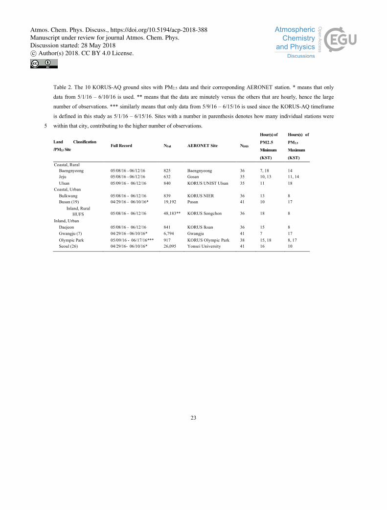
Table 2. The 10 KORUS-AQ ground sites with PM2.5 data and their corresponding AERONET station. * means that only

data from 5/1/16 – 6/10/16 is used. ** means that the data are minutely versus the others that are hourly, hence the large

number of observations. *** similarly means that only data from 5/9/16 – 6/15/16 is used since the KORUS-AQ timeframe

is defined in this study as 5/1/16 – 6/15/16. Sites with a number in parenthesis denotes how many individual stations were

within that city, contributing to the higher number of observations. 5

Land Classification

/PM2.5 Site Full Record NFull AERONET Site N DAYS

Hour(s) of

PM2.5

Minimum

(KST)

Hours(s) of

PM2.5

Maximum

(KST)

Coastal, Rural Baengnyeong 05/08/16 - 06/12/16 825 Baengnyeong 36 7, 18 14 Jeju 05/08/16 - 06/12/16 632 Gosan 35 10, 13 11, 14 Ulsan 05/09/16 - 06/12/16 840 KORUS UNIST Ulsan 35 11 18

Coastal, Urban Bulkwang 05/08/16 - 06/12/16 839 KORUS NIER 36 13 8 Busan (19) 04/29/16 - 06/10/16* 19,192 Pusan 41 10 17

Inland, Rural HUFS 05/08/16 - 06/12/16 48,183** KORUS Songchon 36 18 8

Inland, Urban Daejeon 05/08/16 - 06/12/16 841 KORUS lksan 36 15 8 Gwangju (7) 04/29/16 - 06/10/16* 6,794 Gwangju 41 7 17 Olympic Park 05/09/16 - 06/17/16*** 917 KORUS Olympic Park 38 15, 18 8, 17 Seoul (26) 04/29/16- 06/10/16* 26,095 Yonsei University 41 16 10


24

Figures

Figure 1. a) Map of AERONET sites used in this study. The site marker corresponds to its land classification and its color corresponds to Figure 2. Sites with white markers are not used in Figure 2 due to their limited data availability. Overlaid is AOD 550 nm Dark Target from MODIS Aqua. The daily mean data are used. b) Zoom in of the Seoul Region. 5


25

Figure 2. The AOD diurnal variation and percent departure from daily mean using the full record of AERONET AOD at 550 nm data for the 19 sites of interest.

5


26

Figure 3. The Angstrom Exponent 440-675 nm diurnal variation using the full record of AERONET data for the 19 sites of interest.

5


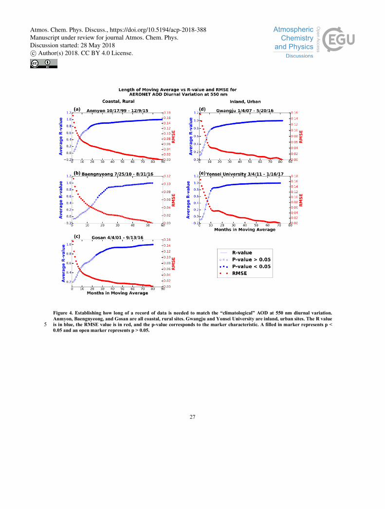
27

Figure 4. Establishing how long of a record of data is needed to match the “climatological” AOD at 550 nm diurnal variation. Anmyon, Baengnyeong, and Gosan are all coastal, rural sites. Gwangju and Yonsei University are inland, urban sites. The R value is in blue, the RMSE value is in red, and the p-value corresponds to the marker characteristic. A filled in marker represents p < 5 0.05 and an open marker represents p > 0.05.


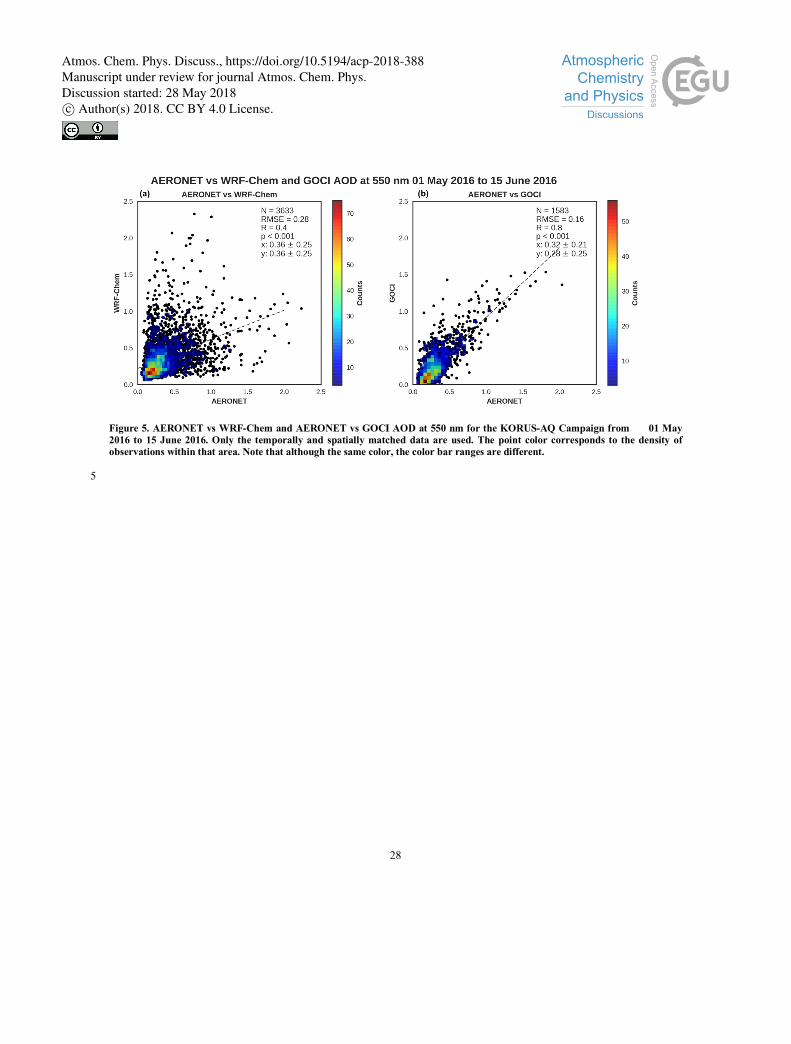
28

Figure 5. AERONET vs WRF-Chem and AERONET vs GOCI AOD at 550 nm for the KORUS-AQ Campaign from 01 May 2016 to 15 June 2016. Only the temporally and spatially matched data are used. The point color corresponds to the density of observations within that area. Note that although the same color, the color bar ranges are different.

5


29

Figure 6. Taylor Diagrams of a) AERONET vs WRF-Chem and b) AERONET vs GOCI


30

Figure 7. The PM2.5 diurnal variation using the 10 KORUS-AQ ground sites that have a corresponding AERONET station nearby. The 24 hour PM2.5 air quality standard in South Korea is 50 mg m-3 and the WHO recommendation is 25 mg m-3.

Figure 8. The diurnal variation of R2 for PM2.5 for the sites in Table 2. 5


31

Figure 9. (a) The diurnal variations for AERONET, WRF-Chem, GOCI, and PM2.5 for the sites in Table 2 using temporally and spatially matched data. (b) The diurnal variation of the observation and WRF-Chem PM2.5 /AOD ratio for the average of the sites in Table 2 using temporally and spatially matched data.


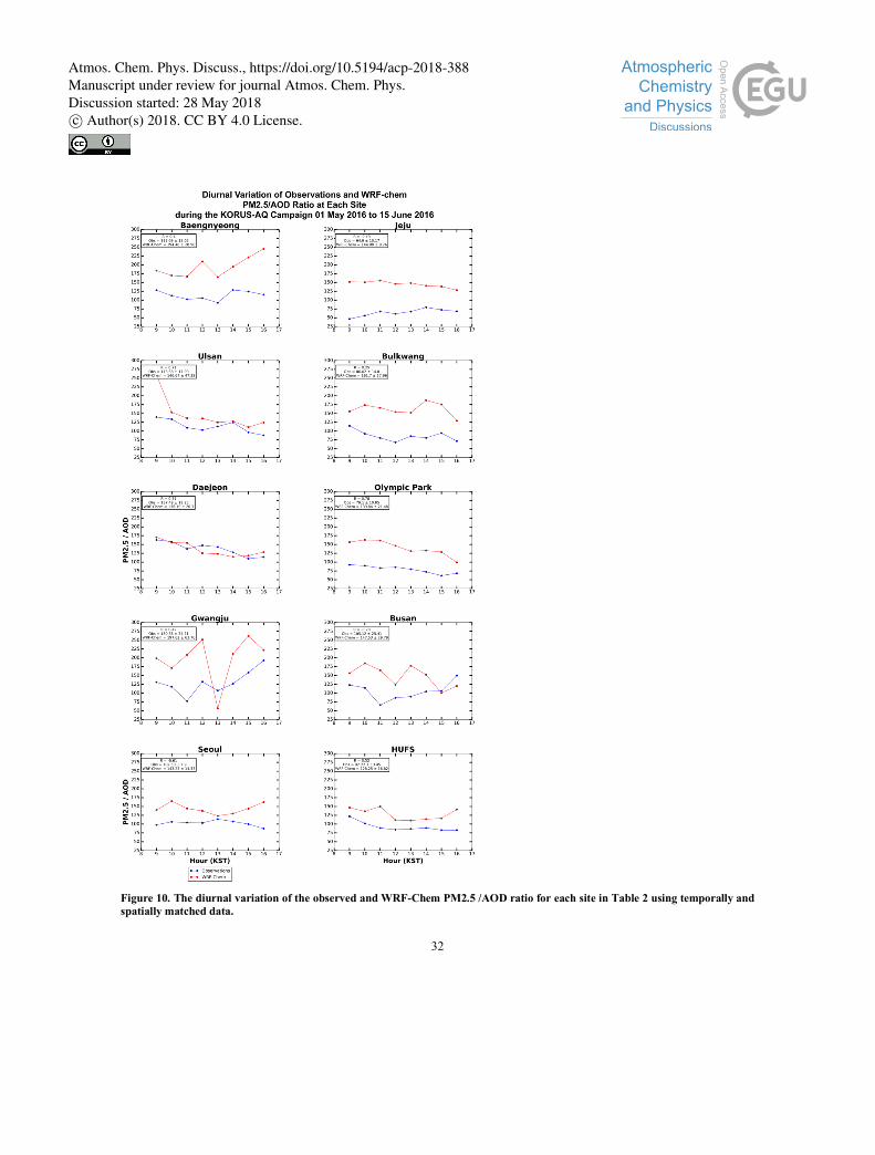
32

Figure 10. The diurnal variation of the observed and WRF-Chem PM2.5 /AOD ratio for each site in Table 2 using temporally and spatially matched data.


discussion started: 28 may 2018 diurnal variation of ... · manuscript under review for journal...

Documents