atmos. chem. phys., 14, 6159–6176

Atmos. Chem. Phys., 14, 6159–6176, 2014www.atmos-chem-phys.net/14/6159/2014/doi:10.5194/acp-14-6159-2014© Author(s) 2014. CC Attribution 3.0 License.

Organic aerosol components derived from 25 AMS data sets acrossEurope using a consistent ME-2 based source apportionmentapproach

M. Crippa 1,*, F. Canonaco1, V. A. Lanz1, M. Äijälä 2, J. D. Allan3,17, S. Carbone4, G. Capes3, D. Ceburnis13,M. Dall’Osto 5, D. A. Day6, P. F. DeCarlo1,** , M. Ehn2, A. Eriksson7, E. Freney8, L. Hildebrandt Ruiz 9,*** , R. Hillamo4,J. L. Jimenez6, H. Junninen2, A. Kiendler-Scharr10, A.-M. Kortelainen 11, M. Kulmala 2, A. Laaksonen11, A.A. Mensah10,**** , C. Mohr1,***** , E. Nemitz12, C. O’Dowd13, J. Ovadnevaite13, S. N. Pandis14, T. Petäjä2, L. Poulain15,S. Saarikoski4, K. Sellegri8, E. Swietlicki7, P. Tiitta11, D. R. Worsnop2,4,11,16, U. Baltensperger1, and A. S. H. Prévôt1

1Laboratory of Atmospheric Chemistry, Paul Scherrer Institute, 5232 PSI Villigen, Switzerland2Department of Physics, P.O. Box 64, University of Helsinki, 00014 Helsinki, Finland3School of Earth, Atmospheric & Environmental Sciences, The University of Manchester, Manchester, UK4Air Quality Research, Finnish Meteorological Institute, P.O. Box 503, 00101 Helsinki, Finland5Institute of Environmental Assessment and Water Research (IDAEA), CSIC, 08034 Barcelona, Spain6Cooperative Institute for Research in Environmental Sciences (CIRES), Boulder, CO, USA7Division of Nuclear Physics, University of Lund, 221 00 Lund, Sweden8Laboratoire de Météorologie Physique, CNRS-Université Blaise Pascal, UMR6016, 63117, Clermont Ferrand, France9Center for Atmospheric Particle Studies, Carnegie Mellon University, 5000 Forbes Ave., Pittsburgh, PA, 15213, USA10Institut für Energie- und Klimaforschung: Troposphäre (IEK 8), Forschungszentrum Jülich GmbH, Jülich, Germany11Department of Environmental Science, Univ. of Eastern Finland, P.O. Box 1627, 70211 Kuopio, Finland12Centre for Ecology and Hydrology, Bush Estate, Penicuik, Midlothian, EH26 0QB, UK13School of Physics & Centre for Climate & Air Pollution Studies, National University of Ireland Galway, Galway, Ireland14Institute of Chemical Engineering Sciences (ICE-HT), Foundation for Research and Technology Hellas (FORTH), Patras,26504, Greece15Leibniz Institute for Tropospheric Research, Permoserstr. 15, 04318 Leipzig, Germany16Aerodyne Research, Inc. Billerica, MA, USA17National Centre for Atmospheric Science, The University of Manchester, Manchester, UK* now at: European Commission, Joint Research Centre, Institute for Environment and Sustainability, Air and Climate Unit,Via Fermi, 2749, 21027 Ispra, Italy** now at: Department of Civil, Architectural, and Environmental Engineering and Department of Chemistry, DrexelUniversity, Philadelphia, PA, 19104, USA*** now at: The University of Texas at Austin, McKetta Department of Chemical Engineering, Austin, TX, 78712, USA**** now at: ETH Zurich, Institute for Atmospheric and Climate Science, Zurich, Switzerland***** now at: Department of Atmospheric Sciences, University of Washington, Seattle WA 98195, USA

Correspondence to:A. S. H. Prévôt ([email protected])

Received: 7 August 2013 – Published in Atmos. Chem. Phys. Discuss.: 5 September 2013Revised: 18 April 2014 – Accepted: 3 May 2014 – Published: 23 June 2014

Published by Copernicus Publications on behalf of the European Geosciences Union.

6160 M. Crippa et al.: Organic aerosol components derived from 25 AMS datasets

Abstract. Organic aerosols (OA) represent one of the ma-jor constituents of submicron particulate matter (PM1) andcomprise a huge variety of compounds emitted by differentsources. Three intensive measurement field campaigns to in-vestigate the aerosol chemical composition all over Europewere carried out within the framework of the European In-tegrated Project on Aerosol Cloud Climate and Air Qual-ity Interactions (EUCAARI) and the intensive campaigns ofEuropean Monitoring and Evaluation Programme (EMEP)during 2008 (May–June and September–October) and 2009(February–March). In this paper we focus on the identifi-cation of the main organic aerosol sources and we define astandardized methodology to perform source apportionmentusing positive matrix factorization (PMF) with the multilin-ear engine (ME-2) on Aerodyne aerosol mass spectrometer(AMS) data. Our source apportionment procedure is testedand applied on 25 data sets accounting for two urban, sev-eral rural and remote and two high altitude sites; thereforeit is likely suitable for the treatment of AMS-related am-bient data sets. For most of the sites, four organic compo-nents are retrieved, improving significantly previous sourceapportionment results where only a separation in primaryand secondary OA sources was possible. Generally, our solu-tions include two primary OA sources, i.e. hydrocarbon-likeOA (HOA) and biomass burning OA (BBOA) and two sec-ondary OA components, i.e. semi-volatile oxygenated OA(SV-OOA) and low-volatility oxygenated OA (LV-OOA).For specific sites cooking-related (COA) and marine-relatedsources (MSA) are also separated. Finally, our work providesa large overview of organic aerosol sources in Europe and aninteresting set of highly time resolved data for modeling pur-poses.

1 Introduction

Atmospheric aerosols negatively affect human health (Popeand Dockery, 2006), reduce visibility, and interact with cli-mate and ecosystems (IPCC, 2007). Among particulate pol-lutants, great interest is dedicated to organic aerosols (OA)since they can represent from 20 to 90 % of the total sub-micron mass (Zhang et al., 2007; Jimenez et al., 2009). Or-ganic aerosols are ubiquitous and are directly emitted by vari-ous sources, including traffic, combustion activities, biogenicemissions, and can also be produced via secondary formationpathways in the atmosphere (Hallquist et al., 2009). Con-straining OA emission sources and understanding their evo-lution and fate in the atmosphere is therefore fundamental todefine mitigation strategies for air quality.

Our work is part of the European Integrated Project onAerosol Cloud Climate and Air Quality Interactions (EU-CAARI), which aims to understand the interactions betweenair pollution and climate. An introduction about project ob-jectives and an overview on the goals reached within the EU-

CAARI project are provided by several papers (Kulmala etal., 2009, 2011; Knote et al., 2011; Fountoukis et al., 2011;Murphy et al., 2012). The coordinated EUCAARI campaignsof 2008 and 2009 provide significantly more aerosol massspectrometer (AMS) data sets to analyze in comparison toprevious efforts (Aas et al., 2012). For the investigationof the aerosol chemical composition and organic aerosol(OA) sources dedicated studies were performed. Nemitz etal. (2014) discuss the organic and inorganic components ofatmospheric aerosols, using AMS measurements performedduring three intensive field campaigns in 2008 and 2009. Ma-jor contribution to the submicron particulate matter (PM1)mass is provided by the organic compounds, which con-tribute from 20 to 63 % to the total mass depending on thesite. Our work deals with the identification and quantifica-tion of organic aerosol sources in Europe using high timeresolution data from aerosol mass spectrometer. Here we fo-cus on the investigation of OA sources applying the positivematrix factorization algorithm (PMF) running on the gener-alized multi-linear engine (ME-2) (Paatero, 1999; Canonacoet al., 2013) to the organic AMS mass spectra from all overEurope.

Currently, only a few studies concerning a broad spatialoverview of OA sources are available in the literature. Zhanget al. (2007) investigated organic aerosol sources in urbanand anthropogenically influenced remote sites in the North-ern Hemisphere, focusing on the discrimination between thetraffic-related and secondary oxygenated OA components.Jimenez et al. (2009) presented an overview of PM1 chemicalcomposition all over the world (including 8 European mea-surement sites) focusing on the identification of OA sourcesusing AMS data. Ng et al. (2010) provided an overview ofOA sources in the Northern Hemisphere, including a broaderspatial domain than Europe and a wide range of locationsaffected by different aerosol sources. Moreover, their ma-jor focus was the investigation of the secondary oxygenatedcomponents and their aging. Lanz et al. (2010) providedan overview of the aerosol chemical composition and OAsources in central Europe focusing on Switzerland, Germany,Austria, France, and Liechtenstein. In all of these studies,the major fraction of PM1 was often represented by organ-ics which consisted, for most of the locations, of oxygenatedOA; however the contribution of primary sources (like trafficand biomass burning) was not always identified especially inrural and remote places. Our work includes 17 measurementsites all over Europe, comprising 25 unit mass resolutionAMS data sets, and represents therefore an unprecedentedoverview of OA sources in Europe. Moreover, the applicationof advanced source apportionment methods allow us to over-come limitations of commonly used source apportionmenttechniques for AMS data, such as the purely unconstrainedpositive matrix factorization (Canonaco et al., 2013). Thepositive matrix factorization (PMF) model does not alwayssucceed since the co-variance of the sources might be largedue to the meteorology and the relative source contributions

Atmos. Chem. Phys., 14, 6159–6176, 2014 www.atmos-chem-phys.net/14/6159/2014/

M. Crippa et al.: Organic aerosol components derived from 25 AMS datasets 6161

which vary too little. This can often be the case at rural andremote sites but it was also shown for an urban backgroundsite in Zurich, for which Lanz et al. (2008) pioneered the useof ME-2 for AMS data. Here, for all measurement sites weare able to clearly separate primary and secondary OA com-ponents, including hydrocarbon-like OA (HOA, associatedwith traffic emissions), biomass burning OA (BBOA), cook-ing (COA) and secondary components (semi-volatile and lowvolatility oxygenated OA, SV-OOA and LV-OOA, respec-tively).

In addition, we provide a standardized source apportion-ment procedure applicable to any measurement site (urban,rural, remote, etc.) guiding source apportionment analysisfor on-line measurements. In fact, when applying multivari-ate methods to AMS data, a critical phase is the evaluationof the results which is strongly affected by subjectivity andobviously depends on the expertise of the researcher. Onegoal of this work is to facilitate the analysis of the modelerdealing with AMS data; additionally, this strategy might beuseful in particular for the analysis of the long-term monitor-ing network data retrieved with the quadrupole or time-of-flight aerosol chemical speciation monitors (ACSM) (Ng etal., 2011b; Fröhlich et al., 2013)

A final motivation of our work is to improve the predic-tion of POA (primary organic aerosol) and SOA (secondaryorganic aerosol) in regional and global models integratingour European overview of OA sources. Our source apportion-ment results are suitable for modeling purposes since under-standing sources and processes of organic aerosols can sub-stantially improve air quality and climate model predictions.Modeling POA and SOA components is challenging and stillcritical due to uncertainties in emission inventories and com-plex atmospheric processing. Including measurements of dif-ferent OA components will improve the evaluation and con-straining of modeling outputs. Our results will help in eval-uating the accuracy of emission inventories (especially con-cerning primary sources) which need better constraints to im-prove regional and global models (Kanakidou et al., 2005; DeGouw and Jimenez, 2009), while SOA sources obtained fromAMS source apportionment could be used to constrain SOAin global chemical transport models (Spracklen et al., 2011).

2 Measurement field campaigns

2.1 Overview of the EUCAARI/EMEP 2008-2009campaigns

Three intensive measurement field campaigns were per-formed during late Spring 2008 (May–June), Fall 2008(September–October) and Winter 2009 (February–March)within the European Integrated Project on Aerosol CloudClimate and Air Quality interactions (EUCAARI) to investi-gate the chemical composition of atmospheric aerosols in Eu-rope among several other objectives (Kulmala et al., 2009).

Figure 1. EUCAARI/EMEP campaigns 2008–2009: measurementperiods.

Aerosol mass spectrometer (AMS) measurements were car-ried out during 26 field campaigns at 17 different sites(see Fig. 1), which are classified as urban (UR, includ-ing Barcelona and Helsinki), rural (RU, including Cabauw,Payerne, Montseny, San Pietro Capofiume, Melpitz, Puijo,Chilbolton, Harwell, K-Puszta, and Vavihill), remote (RE,including Finokalia, Mace Head, and Hyytiälä) and high al-titude (HA, including Jungfraujoch and Puy de Dome) (Ne-mitz et al., 2014). For some of the sites, specific studies werealso published. We refer the reader to Mohr et al. (2012) forthe Barcelona 2009 campaign, to Hildebrandt et al. (2010a,b, 2011) for the Finokalia 2008 and 2009 campaigns, to Men-sah et al. (2012), Li et al. (2013), and Paglione et al. (2013)for the Cabauw 2008 campaign, to Saarikoski et al. (2012)for the San Pietro Capofiume measurements, to Carbone etal. (2014) for the case of Helsinki, to Poulain et al. (2011)for Melpitz, to Dall’Osto et al. (2010) for Mace Head, andto Freney et al. (2011) for Puy de Dome. An overview aboutPM1 aerosol chemical composition is provided in a compan-ion paper by Nemitz et al. (2014), where a detailed discus-sion about measurements setup and data processing is alsoprovided. The average concentrations of PM1 chemical com-ponents as measured by the AMS are also reported in Ta-ble S1 in the Supplement. In this paper we focus on theorganic aerosols (OA) component which represents the ma-jor fraction of submicron particulate matter for most of thesites, ranging between 20 and 63 % of PM1 (concentrationrange: 0.6–8.2 µg m−3), consistent with the values found byJimenez et al. (2009) and Ng et al. (2010). Table 1 sum-marizes the average organic concentration for each site andall the seasons and the relative OA contribution to NR-PM1as measured by the AMS. Figure 2 represents an overviewof the EUCAARI measurement field campaigns focusing onthe organic aerosol sources (an analogous plot for the PM1chemical composition is reported in Nemitz et al. (2014)).For each site the average organic mass concentration of

www.atmos-chem-phys.net/14/6159/2014/ Atmos. Chem. Phys., 14, 6159–6176, 2014


Figure 2. Measurement sites and average organic aerosol source contributions (bars). Measurement sites are classified according to theirlocation as urban (UR), rural (RU), remote (RE) and high altitude (HA). The bar graphs report the average OA source concentrations (y-axisin µg m−3) for the three measurement periods (the chronological order is from left to right: spring 2008, fall 2008 and spring 2009 campaigns,respectively). The identified OA sources are: HOA (hydrocarbon-like OA), BBOA (biomass burning OA), COA (cooking OA), SV-OOA andLV-OOA (semi-volatile and low-volatility oxygenated OA), MSA (methane sulfonic acid) and LOA (local OA).

primary and secondary sources is shown as apportioned byour standard ME-2 approach. Results from the three mea-surement periods are represented with separated bars follow-ing the chronological order from left to right (spring 2008,fall 2008 and spring 2009 campaigns, respectively). Fig-ures S2.1, S2.2, and S2.3 show the time series of the relativecontributions of each OA factor for all the measurement sitesduring the three campaigns. Details about our source appor-tionment strategy exploiting the multi-linear engine (ME-2)are discussed in Sects. 3 and 4.

2.2 Aerosol mass spectrometer measurements

The Aerodyne aerosol mass spectrometer measures size-resolved mass spectra of the non-refractory (NR) PM1aerosol species, where NR species are operationally definedas those that flash vaporize at 600◦C and 10−5 Torr. Blackcarbon, mineral dust, and metals usually cannot be detectedand quantified by the AMS, while Ovadnevaite et al. (2012)shown the possibility to measure sea salt with the AMS. Sev-eral aerosol mass spectrometers were deployed all over Eu-rope during the three intensive EUCAARI field campaigns

Table 1. Average organic concentrations (OA) and their relativecontributions to the NR-PM1 mass measured by the AMS.

Site OA (µg m−3) OA/NR-PM1

Barcelona 8.20 0.50Cabauw 2.60 0.31Finokalia 2.00 0.36Helsinki 2.90 0.38Hyytiälä 1.10 0.45Jungfraujoch 0.66 0.43K-Puszta 5.30 0.45Mace Head 0.85 0.39Melpitz 4.07 0.40Montseny 3.50 0.32Payerne 4.75 0.42Puijo 0.90 0.64Puy de Dome 1.17 0.28San Pietro Capofiume 3.80 0.39Vavihill 3.15 0.39Chilbolton 2.50 0.28Harwell 3.21 0.33



(Nemitz et al., 2014), including Q-AMS (quadrupole AMS)(Jayne et al., 2000), C-ToF-AMS (compact time of flightAMS) (Drewnick et al., 2005) and HR-ToF-AMS (high res-olution time of flight AMS) (DeCarlo et al., 2006).

The general working principle of the AMS is reportedbelow; however the reader should refer to the aforemen-tioned papers for a detailed description of the different AMStypes. Briefly, air is sampled through a critical orifice intoan aerodynamic lens, where the aerosol particles are focusedinto a narrow beam and accelerated to a velocity inverselyrelated to their aerodynamic size. Particles are transmittedinto a high vacuum detection chamber (10−5 Torr) and im-pact on a heated surface (600◦C) where the non-refractoryspecies vaporize. The resulting gas molecules are ionizedby electron impact (EI, 70 eV) and the ions are extractedinto the detection region to be classified by the mass spec-trometer. Details about our AMS measurement quantifica-tion and data treatment (e.g., ionization efficiency calibra-tions, collection efficiency estimation, air corrections, etc.)are described elsewhere (Nemitz et al., 2014). For the evalu-ation of our source apportionment results, black carbon dataobtained from aerosol light absorption measurements per-formed with an aethalometer or a multi angle absorption pho-tometer (MAAP) were also used in our work where available(see Table S3).

3 Organic aerosol source apportionment

3.1 The multilinear engine (ME-2)

Positive matrix factorization (PMF) is the most commonlyused source apportionment method for AMS data (Lanz etal., 2007; Ulbrich et al., 2009; Zhang et al., 2011) to describethe measurements with a bilinear factor model (Paatero andTapper, 1994):

xij =

p∑k=1

gik ∗ fkj + eij (1)

wherexij , gik, fkj andeij represent the matrix elements ofthe measurements (x), time series (g), factor profiles (f), andresiduals (e). The subscripti corresponds to time,j to m/z,k to a discrete factor andp to the number of factors. Themodel solution is found iteratively minimizingQ using theleast squares algorithm:

Q =

m∑i=1

n∑j=1

(eij

σij

)2

, (2)

whereσij are the measurement uncertainties.The model solution is not unique due to rotational am-

biguity (Paatero et al., 2002), in fact the product of the ro-tated matrixG andF (G =G ·T andF = T −1

·F ) is equal tothe product of the corresponding unrotated matrix which alsoprovides the same value of the object functionQ. In order to

reduce rotational ambiguity within the ME-2 algorithm, theuser can add a priori information into the model (e.g., sourceprofiles), so that it does not rotate and it provides a ratherunique solution (Paatero and Hopke, 2009).

We perform organic aerosol source apportionment usingthe multi-linear engine (ME-2) algorithm (Paatero, 1999) im-plemented within the toolkit SoFi (Source Finder) developedby Canonaco et al. (2013) at Paul Scherrer Institute. Simi-larly to the PMF solver (Paatero and Tapper, 1994), the ME-2solver (Paatero, 1999) executes the positive matrix factoriza-tion algorithm. However, the user has the advantage to sup-port the analysis by introducing a priori information in formof known factor time series and / or factor profiles, for exam-ple within the so-calleda value approach (see Eqs. (3a) and(3b)). Thea value (ranging from 0 up to values larger than1) determines how much the resolved factors (fj,solution) andgi,solution) are allowed to vary from the input ones (fj , gi), asdefined in Eq. (3a) and (3b) (Canonaco et al., 2013). In ourwork we only constrained the mass spectra represented byf .

fj,solution= fj ± α · fj (3a)

gi,solution= gi ± α · gi (3b)

For example, ifa = 0.1 when constraining a mass spectralprofile, all of them/z’s in the fit profile can vary as muchas−10 % to+10 % of the input constraining mass spectrumprofile.

In our work, a constanta value is applied to the entire con-strained mass spectra (MS); however a softer constrainingtechnique is provided by the pulling approach (Paatero andHopke, 2009; Brown et al., 2012), which is available withinthe SoFi package (Canonaco et al., 2013) and which is ex-plained in more detail in Canonaco et al. (2014b).

The ME-2 solver is here successfully applied to the timeseries of the unit mass resolution organic mass spectra mea-sured by the AMS, including for most of the sitesm/z upto 200 (for a few sites the analysis was performed only upto m/z 150 due to the low signal to noise ratio (SNR) ob-served). Data are first averaged to 15–30 minute time resolu-tion and after performing the source apportionment analysisthey are averaged to 1 hour for modeling purposes. The errormatrix preparation before running the source apportionmentalgorithm is performed following the procedure introducedby Ulbrich et al. (2009). Briefly, a minimum counting er-ror of 1 ion is applied,m/z with SNR between 2 and 0.2(weak variables) are downweighted by a factor of 2, whilebad variables (SNR<0.2) are downweighted by a factor of 10(Paatero and Hopke, 2003; Ulbrich et al., 2009). Moreover,based on the AMS fragmentation table, some organic massesare not directly measured but calculated as a fraction of theorganic signal atm/z 44 (Allan et al., 2004); therefore theerrors of thesem/z 44 dependent peaks are downweighted(Ulbrich et al., 2009).



3.2 A standardized source apportionment strategy

In this section we provide technical guidelines to performa standard source apportionment analysis on AMS data inorder to identify well known organic aerosol sources, likehydrocarbon-like (HOA), biomass burning (BBOA), cook-ing (COA) and oxygenated components (OOA), but also site-specific sources. Our approach is particularly relevant forrural locations where the temporal variability of emissionsources is less distinct and where the aging processes aredominant compared to fresh emissions. A detailed descrip-tion of the main features of these OA sources (source pro-file, diurnal patterns, etc.) is presented in Sect. 4. Here, wedefine first our source apportionment strategy and then weprovide details about the application of this methodology onthe EUCAARI-EMEP data. Finally, some technical exam-ples concerning the data treatment and interpretation are alsoreported in Sects. 3.2.2 and 3.2.3.

3.2.1 Technical guidelines

Within our work we define a standardized methodology toperform source apportionment on AMS data using the ME-2 algorithm with the aforementioned SoFi toolkit (Paatero,1999; Canonaco et al., 2013). The sequential steps of themethodology are reported below:

1. Unconstrained run (PMF).

2. Constrain the HOA mass spectrum (MS) with a lowa value (e.g.,a =0.05–0.1) and test various number offactors.

3. Look for BBOA (if not identified yet): constrain theBBOA MS if f60 (i.e., the fraction ofm/z 60 to the to-tal organic mass) is above background level and checktemporal structures like diurnal increases in the eveningduring the cold season due to domestic wood burning(suggesteda value = 0.3–0.5).

4. Look for COA (if cooking not found yet): check thef55–f57 plot for cooking evidence (wheref55 andf57are the fraction ofm/z 55 andm/z 57 to the total or-ganic mass respectively; see Mohr et al., 2012). Fix it inany case and check its diurnal pattern (the presence ofthe meal hour peaks is necessary to support it at least inurban areas).

5. Residual analysis: a structure in the residual diurnalsmight indicate possible sources not separated yet by themodel (refer to Section 3.2.3). For each step the resid-ual plots should always be consulted in order to evalu-ate whether the constrained profile(s) has(have) causedstructures in the residuals. If so, the constrained profileshould be tested with a higher scalara value.

6. In general the OOA components are not fixed, but areleft as 1 to 3 additional unconstrained factors.

Our approach starts with an unconstrained run, where noa priori information concerning the source mass spectra isadded. This first step is important because it reveals the possi-bility of separation for several OA components with PMF. Italso gives the user an idea of the number of possible sourcesfor that site, even though they might not be clearly sepa-rated yet. If the HOA mass spectrum is not identified in thefirst step (e.g., considering from 1 to 5 unconstrained fac-tors), the user should fix the HOA mass spectrum with thea value approach and, to evaluate the presence of this sourceinto the data set, investigate its diurnal pattern and correla-tion with available external tracers (e.g., black carbon, NOx,etc.). At this step several constrained runs are required vary-ing the number of unconstrained factors (e.g., from 3 to 5)in order to investigate the presence of other possible sources(e.g., BBOA, COA, secondary components and possibly spe-cific site-related factors). Moreover, the user should performa sensitivity analysis on thea value associated with the HOAMS in order to define a range of possible solutions. A de-tailed discussion about the sensitivity analysis is reported inSect. 4.5. If the user is unable to identify a biomass burningrelated source within step 2, the investigation of the diurnalpattern of a specific organic tracer for levoglucosan and pri-mary biomass combustion species (f60 = m/z 60 / OA) (Al-farra et al., 2007) can reveal the presence of BBOA at thesite (e.g., increasing contribution off60 during the eveningsuggests the use of biomass burning for domestic heatingpurposes). In addition, it is important to study the variabil-ity of f60 above background levels, which is reported to be0.3 %± 0.06 % (DeCarlo et al., 2008; Aiken et al., 2009; Cu-bison et al., 2011). Finally, a primary OA source especiallyimportant in urban areas is cooking (COA) (Slowik et al.,2010; Allan et al., 2010; Sun et al., 2011; Mohr et al., 2012;Crippa et al., 2013). The cooking contribution is not easilyresolved even for urban sites due to the similarity of its massspectrum with the one of HOA in unit mass resolution. So af-ter identifying HOA and BBOA, the user should constrain theCOA MS with a rather lowa value (e.g.,a =0.05). To inter-pret the retrieved factor as a cooking-related source, its diur-nal pattern should show two peaks corresponding to the mealhours at least in urban or semi-urban sites. As demonstratedin Fig. 6 of Mohr et al. (2012), thef55 vs.f57 plot can pro-vide further evidence of COA in urban sites strongly affectedby cooking activities. In fact, the triangular space definedby Mohr et al. (2012) allows the identification of cooking-influenced OA for points lying on the left hand side of thistriangle which are dominated byf55 (and therefore cook-ing emissions) compared to points dominated by the trafficsource (lying on the right hand side of the triangle).

For specific sites (e.g., coastal locations, etc.) differentsources from continental urban and rural locations can beexpected. Therefore any a priori knowledge about specificOA sources should be constrained when running the ME-2 engine, to drive the model in finding local sources, of-ten characterized by low contribution in mass and reduced



temporal variability. Technical examples are provided inSect. 3.2.2.

At each step of the discussed methodology, it is importantto evaluate how the residuals vary moving from one step tothe other, and within a single phase varying the number offactors. After fixing HOA and BBOA (step 3), the investi-gation of the average diurnal variation of the residuals canhighlight the presence of unresolved sources by the model(refer to Sect. 2.3.3 for further discussion).

When using the ME-2 algorithm for fixing source profiles,the user must carefully validate the obtained results since agood solution is not selected based on the possibility to re-trieve a constrained profile (which is expected as output ofthe model), but on several concurrent validation procedures.The toolkit SoFi created by Canonaco et al. (2013) greatlyhelps in performing all the suggested steps of our sourceapportionment methodology and provides several metricsto evaluate the quality of the chosen solution (e.g., cor-relation with external data time series and mass spectra,detailed residuals analysis, explained/unexplained variationplots etc.) and also an efficient comparison of different so-lutions (see SoFi manual,http://www.psi.ch/acsm-stations/me-2).

3.2.2 Application to the EUCAARI-EMEP data

The previously mentioned procedure is successfully appliedon the 25 available organic AMS data sets and thereforeit provides a consistent methodology. Deploying the ME-2solver allows the discrimination of traffic and biomass burn-ing within the primary sources and of two OOA componentsfor the secondary fraction for most of the sites. In order toperform a value runs within the ME-2 solver, it is neces-sary to select reference mass spectra to be constrained in themodel. Due to the similar features of the HOA and COA massspectra, in our work we choose the HOA and COA massspectra identified in Paris by Crippa et al. (2013) as a ref-erence, because of the significant contribution of the cook-ing source to the total OA mass and its strong diurnal pat-tern at that site. Solutions from other sites may have cook-ing and HOA mixed to some extent. For the BBOA refer-ence mass spectrum we adopt the one introduced by Ng etal. (2011a) since it is considered representative of averagedambient biomass burning conditions. A detailed sensitivityanalysis investigating the impact of the input MS on the fi-nal solution is already ongoing and will be fully addressed inCanonaco et al. (2014a).

Additionally, for the two marine measurement sites (MaceHead and Finokalia), a methane sulfonic acid (MSA) fac-tor is used too (see Sect. S5). First, a relatively clean MSAMS is obtained through an unconstrained PMF run for theMace Head 2008 late spring campaign (see Fig. S5 of thesupplementary material), during which high biological activ-ity is expected (Dall’Osto et al., 2010). As a second step,this MSA MS is used as input to the algorithm for the two

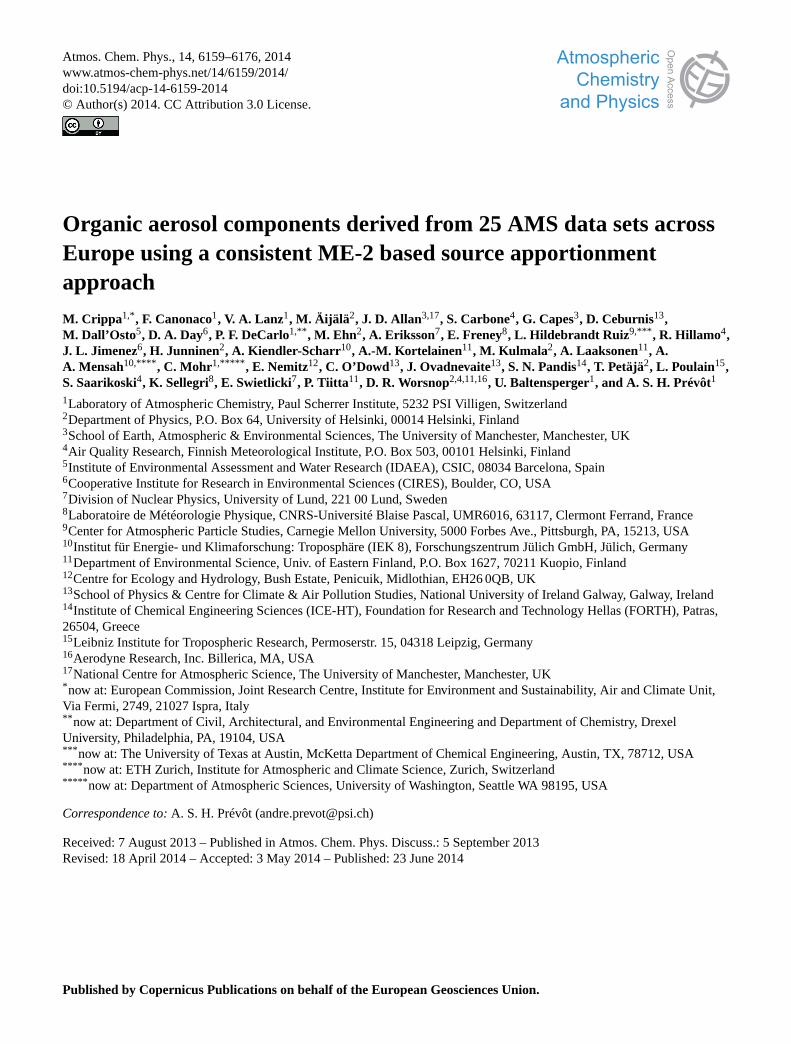
Figure 3. Comparison of the diurnal pattern of the Q-value for the5-factor solution constraining HOA-BBOA or HOA-BBOA-COA(Barcelona 2009). The structure in the scaled residuals suggests thepresence of additional sources.

other field campaigns (Finokalia 2008 and Mace Head 2009).The separation of this factor is a challenge for the uncon-strained PMF, due to reduced biological activity during earlyspring in Mace Head and weak marine influence for the sitein Crete. Finally, in order to provide a complete overview ofthe EUCAARI 2008–2009 data, the PMF solution describedin this paper for the Finokalia 2009 campaign is reported inthis work. Our standardized procedure could not be appliedto this data set due to specifics of the data pre-treatment andthe presence of unusual local sources.

3.2.3 Technical example of structure in the residuals

As discussed in Sect. 3.2.1, the analysis of the residual struc-ture is fundamental to understand how the model solutionvaries when adding more factors and which variables and/orevents get more explained. Figure 3 shows how the aver-age diurnal profile of the scaled residuals (Q) for Barcelonachanges for the 5-factor solution run when constraining HOAand BBOA and when additionally constraining COA. In thefirst case, theQ diurnal shows two prominent peaks corre-sponding to the meal hours in Barcelona (Mohr et al., 2012),which suggests the presence of a possible cooking source notresolved yet by the model. Therefore the residual analysisprovides an additional good reason to use the ME-2 algo-rithm to also constrain a cooking source. After constrainingthe COA mass spectrum in the model, the performance ofthe model improves since the structure observed in the diur-nal profile of the residuals disappears.

4 Results and discussion

4.1 Primary and secondary OA source contributions

The standardized source apportionment strategy introducedin Sect. 3.2 is systematically applied to the 25 available


http://www.psi.ch/acsm-stations/me-2

http://www.psi.ch/acsm-stations/me-2


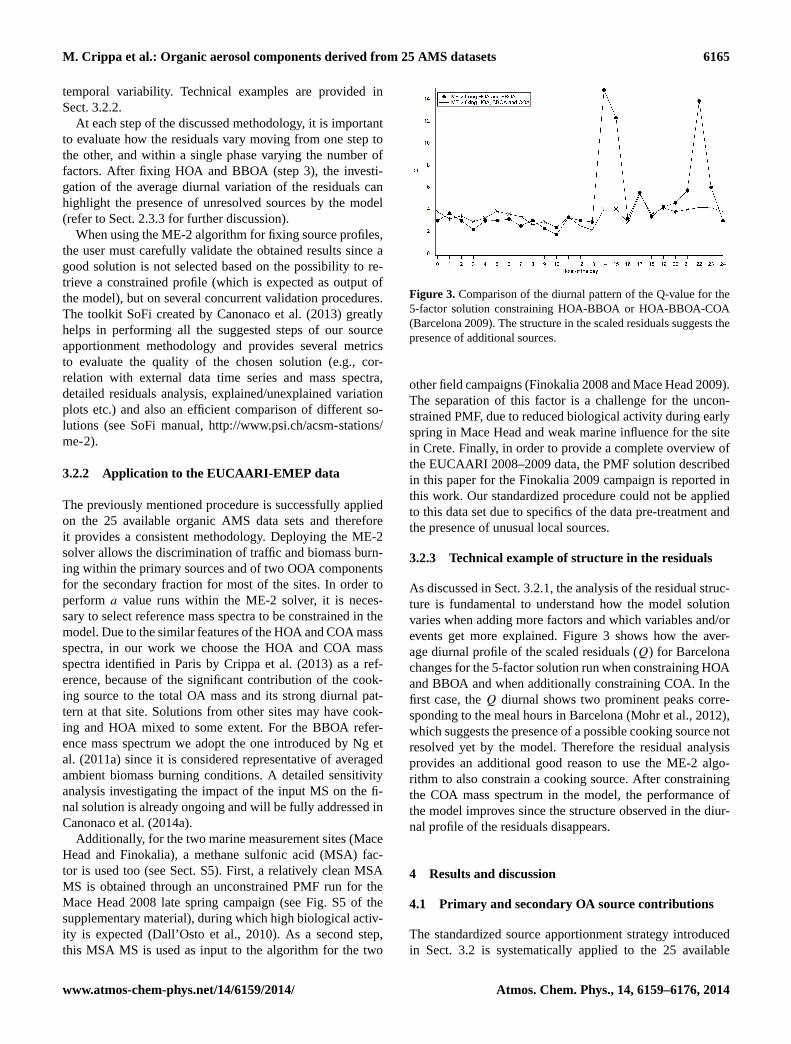
Table 2. Relative contributions of the identified organic components to the total OA. Note that only main organic sources in common formost of the sites are reported (HOA, BBOA, SV-OOA and LV-OOA).

Site Spring 2008 Fall 2008 Spring 2009HOA BBOA SV-OOA LV-OOA HOA BBOA SV-OOA LV-OOA HOA BBOA SV-OOA LV-OOA

Barcelona 0.24 0.08 0.20 0.29Cabauw 0.14 0.10 0.22 0.39 0.19 0.10 0.34 0.36Finokalia 0.04 – 0.33 0.58 0.66Helsinki 0.16 0.14 0.20 0.51Hyytiälä 0.06 0.04 0.42 0.48 0.03 0.05 0.28 0.65Jungfraujoch 0.06 0.11 – 0.83K-Puszta 0.12 0.11 0.33 0.44Mace Head 0.12 0.16 0.28 0.39 0.12 0.27 0.59Melpitz 0.05 – 0.51 0.44 0.08 0.14 0.35 0.43 0.09 0.11 0.28 0.52Montseny 0.07 0.09 – 0.83Payerne 0.06 0.12 0.28 0.53 0.07 0.09 0.27 0.57Puijo 0.22 – – 0.78Puy de Dome 0.01 0.09 0.55 0.35 0.06 0.18 0.37 0.39San Pietro Capofiume 0.10 0.12 0.28 0.50Vavihill 0.20 0.12 – 0.68 0.21 0.10 0.50 0.19Chilbolton 0.20 0.20 0.19 0.40Harwell 0.07 0.13 0.32 0.48

AMS data sets, consisting of the AMS matrices with theorganic mass spectra over time and the corresponding er-rors. Table S2 reports the comparison of the number of OAcomponents identified with thea value approach in com-parison with the unconstrained run (PMF) (Ulbrich et al.,2009), highlighting in red the constrained source mass spec-tra. The unconstrained PMF often cannot provide a clear sep-aration of OA sources in rural and remote sites (Zhang etal., 2007; Jimenez et al., 2009). This may also happen at ur-ban background sites where the effect of meteorology canstill be dominant compared to the source temporal variabil-ity (Lanz et al., 2008; Canonaco et al., 2013). In our 25 datasets, unconstrained PMF allows mainly the identification ofPOA (often including HOA and BBOA in one factor typi-cally characterized by high signal atm/z 44 and 60) and SOAsources (refer to Table S2). Even when HOA is identified,it is often not clean due to the high contribution ofm/z 44(which should be rather small for primary traffic emissions).In some cases it is only possible to separate two secondaryoxygenated components, but no primary source is retrieved,although expected.

On the contrary, with our approach, primary and sec-ondary OA sources are retrieved for all the analyzed datasets, including traffic (HOA), cooking (COA) and biomassburning (BBOA) as primary sources, and methane sulfonicacid (MSA), semi-volatile and low-volatility oxygenated OA(SV-OOA and LV-OOA) as secondary components. For theCabauw 2008 and Finokalia 2009 data sets the contributionof local (site specific) sources is also observed. The ME-2solution for the Cabauw 2008 campaign includes a site spe-cific factor (named here LOA, local organic aerosol) whichis interpreted to be hulis-related (humic-like substances), aswidely explained in Paglione et al. (2013). These results rep-resent a great improvement in the source apportionment field,since we demonstrate the possibility to identify several pri-

Figure 4. Relative organic source contributions (ME-2 results). Ontop of each bar the average organic concentration (in µg m−3) is alsoreported. Site specific sources are classified as LOA (local organicaerosols) and include HULIS-related OA (humic-like substances)for Cabauw (Paglione et al., 2013), while amines and local sourcesfor Finokalia (Hildebrandt et al., 2011).

mary and secondary OA components even at rural locationswhere the POA factors often contribute less than 10 % of theOA. Comparisons with previously published PMF solutions(mainly from HR-PMF data) for specific sites are reported inSect. S3 of the supplementary material.

Our methodology combines the advantages of the chem-ical mass balance and the positive matrix factorization ap-proach. In fact, the a priori knowledge of well-known sourceprofiles (e.g., from primary sources) drives the source ap-portionment algorithm in finding an optimal solution for the



Figure 5. Relative organic source contributions as a function of total organic concentrations. Average plot over all the seasons and rural sites(a), Barcelona only(b), and average plot for marine sites(c).

model, while less constrained components (e.g., secondaryOA) are allowed to freely vary (similarly to the unconstrainedPMF case). However, our approach should provide consistentresults with the unconstrained PMF case, where an optimalsolution could be also identified by the means of other tech-niques such as e.g., a significant number of seeds, individ-ual rotations or by reweighting specific uncertainties, etc.,although requiring often very high time efforts and a lot ofexpertise on the user side.

Figure 4 summarizes the average organic aerosol con-centration and the average relative contribution of each OAsource for each site (see also Table 2). For all sites andcampaigns it is possible to separate a hydrocarbon-like OAfactor (average equal to 11± 6 % of OA), whose contribu-tion on average ranges from 3 % to 24 % to the total OAmass. The HOA average concentration ranges between 0.1and 2.1 µg m−3 depending on the site location and campaign.Although Puijo is classified as rural site, it has nearly thelargest HOA fraction since located on a hill at 2 km from thecity center of Kuopio (population 97000) which is a sourceof HOA and few point sources (Leskinen et al., 2012; Hao etal., 2013). However, in absolute terms, HOA concentrationsin Puijo are rather low (0.2 µg m−3), while at sites with hightotal OA concentrations the absolute HOA amount is highercompared to rural sites.

Biomass burning is identified in 22 data sets and is associ-ated with a mix of domestic heating during cold periods andopen fires (e.g., agricultural, forest and gardening waste) andbarbecuing activities etc. The BBOA contribution to the total

OA mass varies on average between 5 and 27 % (correspond-ing to 0.1–0.8 µg m−3) with an average relative contributionto the total OA mass equal to 12± 5 %. At 3 sites (Melpitzspring 2008, Puijo fall 2008 and Finokalia spring 2008)f60is close to or below the background values and the BBOAis regarded as negligible. Major contribution to total OA de-rives from secondary sources, which are classified here basedon their degree of oxygenation as SV-OOA and LV-OOA andwhich contribute on average 34± 11 % and 50± 16 % to thetotal OA mass, respectively.

Cooking contributes on average∼15 % to the total OAmass in Barcelona, consistent with AMS ambient measure-ments performed in European urban areas like Zurich, Paris,London, etc. (Mohr et al., 2012; Canonaco et al., 2013;Crippa et al., 2013; Allan et al., 2010). Finally, MSA con-tributes from 2 % to 6 % to the total OA mass in the twomarine sites (Mace Head and Finokalia), similarly to the val-ues reported by Dall’Osto et al. (2010) and Ovadnevaite etal. (2014).

Figure 5 is an alternative method to summarize source ap-portionment results, in fact instead of reporting average con-centrations of the sources, it reports the relative OA sourcecontribution vs. the OA concentration for all the rural, ma-rine and urban sites, highlighting the role of specific sourceswithin different concentration ranges (average over 21, 1 and3 data sets for panel a, b and c, respectively). The numberof measurements happening for each concentration bin isreported (black line with markers) and shows a decreasing



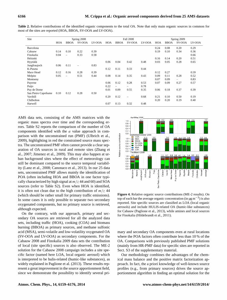
Figure 6.Diurnal profiles of organic aerosol components. Mean values (± standard deviation) for OA components are shown for the differentseasons and all sites.

trend for higher concentration. The last concentration bin in-cludes all data points above that concentration.

For rural sites (see Fig. 5a), the HOA contribution de-creases with increasing OA concentrations, while the BBOAcontribution is very small for very low concentrations(<1 µg m−3), but stable over the rest of the concentrationrange. No general pattern can be observed for the two sec-ondary components. However the LV-OOA fraction seemsto increase at higher concentration. For an urban site likeBarcelona (see Fig. 5b), traffic is a significant source bothat low and high OA concentrations, while the semi-volatileoxygenated component is rather low. However, the differen-tiation between SV- and LV-OOA is highly dependent on theoxidation processes in the atmosphere, geographical positionof the measurement site, season, meteorological conditions,etc., therefore our conclusions for the Barcelona site mightnot have general validity. Figure 5c shows the fractional con-tribution of OA sources as a function of total OA concentra-tion for marine sites. An interesting feature is the high rel-ative contribution of MSA at very low OA concentrations(below 1 µg m−3), where both the primary OA sources andthe LV-OOA fraction are small. Figure 5 highlights the im-portance of comparing models and measurements in differentconcentration ranges instead of only e.g., the average contri-butions. An obvious example is Mace Head where the contri-bution of sources at low concentrations from the Atlantic arevery different from situations when the station is downwindof European pollution.

4.2 Evaluation of results

The interpretation of the retrieved source apportionment fac-tors as organic aerosol sources is based on correlations withexternal data (see Table S3), the investigation of their diur-

nal pattern (Fig. 5) and the source mass spectra compari-son with reference ones (refer to Sect. 4.3 for further dis-cussion). However, presenting all details about the evalua-tion of the source apportionment results for each campaignis beyond the scope of this paper. HOA typically corre-lates with black carbon, which is co-emitted by the samesource; biomass burning correlates with the organic frag-ment atm/z 60 (org60) which corresponds mainly to the ionC2H4O+

2 and has been shown to be a good tracer for biomassburning (Alfarra et al., 2007; DeCarlo et al., 2008; Aikenet al., 2009). However, in marine environment,m/z 60 isusually dominated by Na37Cl (Ovadnevaite et al., 2012). Tofurther evaluate the interpretation of primary sources withinthe selected solution, source-specific ratios can be calculated(e.g., HOA / CO, HOA/BC and HOA / NOx) and comparedwith literature studies. However, in our work this approachcould not be systematically applied due to the lack of externaldata. Bilinear regression (Allan et al., 2010) can be used toestimate these ratios also in the presence of multiple sources;however, this method is more applicable to a single data setrather than an overview of 25 data sets across Europe.

The secondary OA components are compared with thesecondary inorganic species: the SV-OOA time series areexpected to correlate with nitrate (NO3) due to the highervolatility of this component and its partitioning behavior withtemperature, while the LV-OOA time series are correlatedwith sulfate (SO4) since it represents a less volatile fraction(Lanz et al., 2007). However, depending on the specific fea-tures of the SV-OOA and LV-OOA components, associatedwith their origin and processing in the atmosphere, their cor-relations with the secondary inorganic species might be notvery high (Table S3). Finally, to further validate our sourceapportionment results, we investigated the diurnal patternof the identified sources. In order to remove the effect of



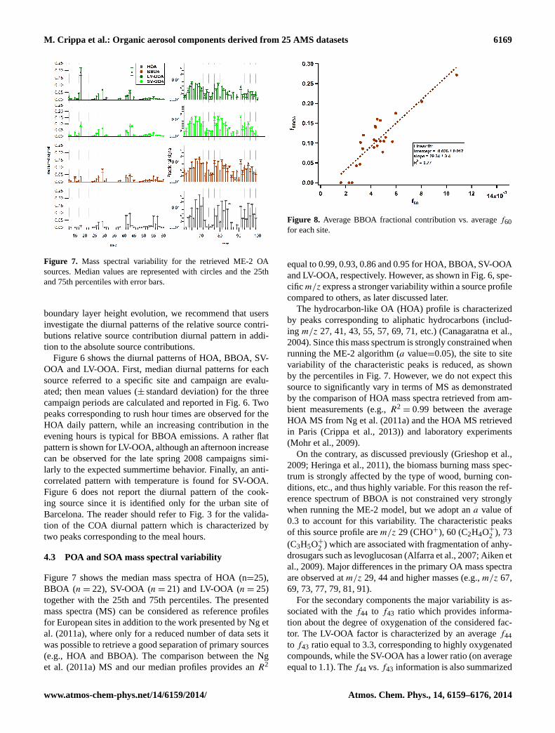
Figure 7. Mass spectral variability for the retrieved ME-2 OAsources. Median values are represented with circles and the 25thand 75th percentiles with error bars.

boundary layer height evolution, we recommend that usersinvestigate the diurnal patterns of the relative source contri-butions relative source contribution diurnal pattern in addi-tion to the absolute source contributions.

Figure 6 shows the diurnal patterns of HOA, BBOA, SV-OOA and LV-OOA. First, median diurnal patterns for eachsource referred to a specific site and campaign are evalu-ated; then mean values (± standard deviation) for the threecampaign periods are calculated and reported in Fig. 6. Twopeaks corresponding to rush hour times are observed for theHOA daily pattern, while an increasing contribution in theevening hours is typical for BBOA emissions. A rather flatpattern is shown for LV-OOA, although an afternoon increasecan be observed for the late spring 2008 campaigns simi-larly to the expected summertime behavior. Finally, an anti-correlated pattern with temperature is found for SV-OOA.Figure 6 does not report the diurnal pattern of the cook-ing source since it is identified only for the urban site ofBarcelona. The reader should refer to Fig. 3 for the valida-tion of the COA diurnal pattern which is characterized bytwo peaks corresponding to the meal hours.

4.3 POA and SOA mass spectral variability

Figure 7 shows the median mass spectra of HOA (n=25),BBOA (n = 22), SV-OOA (n = 21) and LV-OOA (n = 25)together with the 25th and 75th percentiles. The presentedmass spectra (MS) can be considered as reference profilesfor European sites in addition to the work presented by Ng etal. (2011a), where only for a reduced number of data sets itwas possible to retrieve a good separation of primary sources(e.g., HOA and BBOA). The comparison between the Nget al. (2011a) MS and our median profiles provides anR2

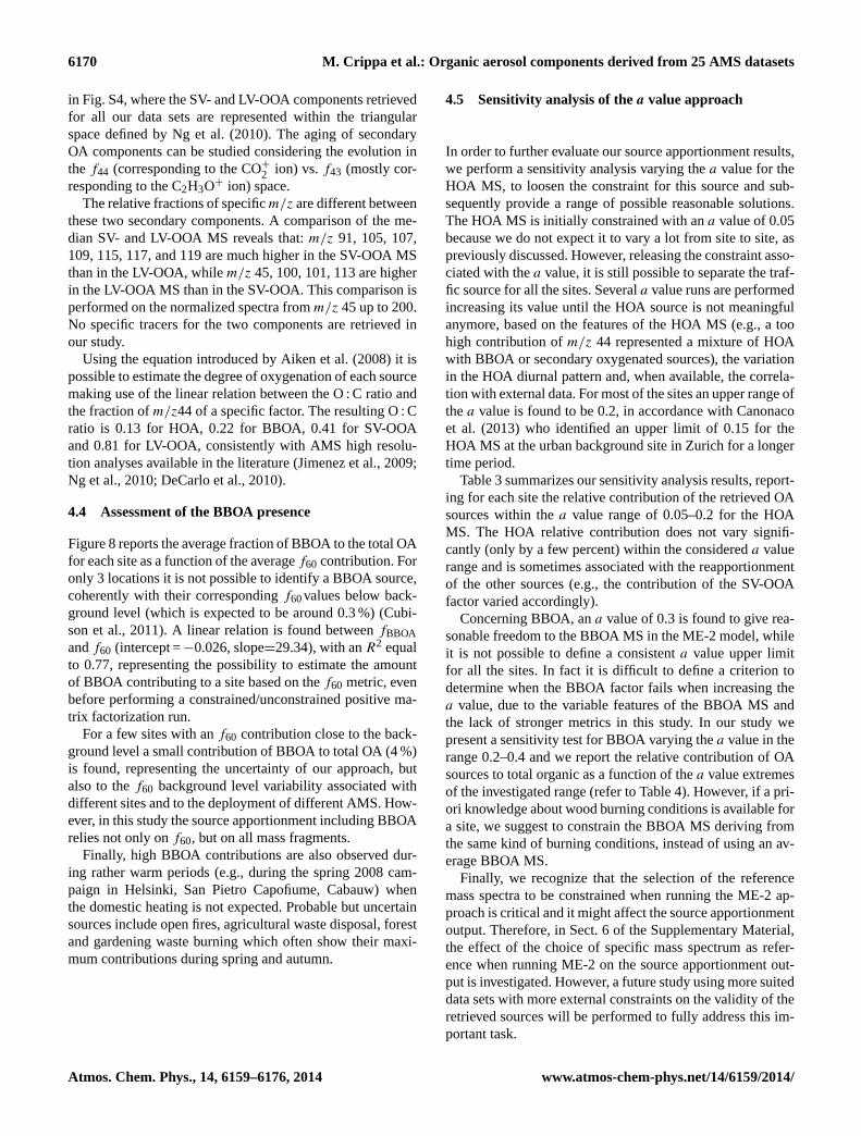
Figure 8. Average BBOA fractional contribution vs. averagef60for each site.

equal to 0.99, 0.93, 0.86 and 0.95 for HOA, BBOA, SV-OOAand LV-OOA, respectively. However, as shown in Fig. 6, spe-cific m/z express a stronger variability within a source profilecompared to others, as later discussed later.

The hydrocarbon-like OA (HOA) profile is characterizedby peaks corresponding to aliphatic hydrocarbons (includ-ing m/z 27, 41, 43, 55, 57, 69, 71, etc.) (Canagaratna et al.,2004). Since this mass spectrum is strongly constrained whenrunning the ME-2 algorithm (a value=0.05), the site to sitevariability of the characteristic peaks is reduced, as shownby the percentiles in Fig. 7. However, we do not expect thissource to significantly vary in terms of MS as demonstratedby the comparison of HOA mass spectra retrieved from am-bient measurements (e.g.,R2

= 0.99 between the averageHOA MS from Ng et al. (2011a) and the HOA MS retrievedin Paris (Crippa et al., 2013)) and laboratory experiments(Mohr et al., 2009).

On the contrary, as discussed previously (Grieshop et al.,2009; Heringa et al., 2011), the biomass burning mass spec-trum is strongly affected by the type of wood, burning con-ditions, etc., and thus highly variable. For this reason the ref-erence spectrum of BBOA is not constrained very stronglywhen running the ME-2 model, but we adopt ana value of0.3 to account for this variability. The characteristic peaksof this source profile arem/z 29 (CHO+), 60 (C2H4O+

2 ), 73(C3H5O+

2 ) which are associated with fragmentation of anhy-drosugars such as levoglucosan (Alfarra et al., 2007; Aiken etal., 2009). Major differences in the primary OA mass spectraare observed atm/z 29, 44 and higher masses (e.g.,m/z 67,69, 73, 77, 79, 81, 91).

For the secondary components the major variability is as-sociated with thef44 to f43 ratio which provides informa-tion about the degree of oxygenation of the considered fac-tor. The LV-OOA factor is characterized by an averagef44to f43 ratio equal to 3.3, corresponding to highly oxygenatedcompounds, while the SV-OOA has a lower ratio (on averageequal to 1.1). Thef44 vs.f43 information is also summarized



in Fig. S4, where the SV- and LV-OOA components retrievedfor all our data sets are represented within the triangularspace defined by Ng et al. (2010). The aging of secondaryOA components can be studied considering the evolution inthef44 (corresponding to the CO+2 ion) vs.f43 (mostly cor-responding to the C2H3O+ ion) space.

The relative fractions of specificm/z are different betweenthese two secondary components. A comparison of the me-dian SV- and LV-OOA MS reveals that:m/z 91, 105, 107,109, 115, 117, and 119 are much higher in the SV-OOA MSthan in the LV-OOA, whilem/z 45, 100, 101, 113 are higherin the LV-OOA MS than in the SV-OOA. This comparison isperformed on the normalized spectra fromm/z 45 up to 200.No specific tracers for the two components are retrieved inour study.

Using the equation introduced by Aiken et al. (2008) it ispossible to estimate the degree of oxygenation of each sourcemaking use of the linear relation between the O : C ratio andthe fraction ofm/z44 of a specific factor. The resulting O : Cratio is 0.13 for HOA, 0.22 for BBOA, 0.41 for SV-OOAand 0.81 for LV-OOA, consistently with AMS high resolu-tion analyses available in the literature (Jimenez et al., 2009;Ng et al., 2010; DeCarlo et al., 2010).

4.4 Assessment of the BBOA presence

Figure 8 reports the average fraction of BBOA to the total OAfor each site as a function of the averagef60 contribution. Foronly 3 locations it is not possible to identify a BBOA source,coherently with their correspondingf60values below back-ground level (which is expected to be around 0.3 %) (Cubi-son et al., 2011). A linear relation is found betweenfBBOAandf60 (intercept =−0.026, slope=29.34), with anR2 equalto 0.77, representing the possibility to estimate the amountof BBOA contributing to a site based on thef60 metric, evenbefore performing a constrained/unconstrained positive ma-trix factorization run.

For a few sites with anf60 contribution close to the back-ground level a small contribution of BBOA to total OA (4 %)is found, representing the uncertainty of our approach, butalso to thef60 background level variability associated withdifferent sites and to the deployment of different AMS. How-ever, in this study the source apportionment including BBOArelies not only onf60, but on all mass fragments.

Finally, high BBOA contributions are also observed dur-ing rather warm periods (e.g., during the spring 2008 cam-paign in Helsinki, San Pietro Capofiume, Cabauw) whenthe domestic heating is not expected. Probable but uncertainsources include open fires, agricultural waste disposal, forestand gardening waste burning which often show their maxi-mum contributions during spring and autumn.

4.5 Sensitivity analysis of thea value approach

In order to further evaluate our source apportionment results,we perform a sensitivity analysis varying thea value for theHOA MS, to loosen the constraint for this source and sub-sequently provide a range of possible reasonable solutions.The HOA MS is initially constrained with ana value of 0.05because we do not expect it to vary a lot from site to site, aspreviously discussed. However, releasing the constraint asso-ciated with thea value, it is still possible to separate the traf-fic source for all the sites. Severala value runs are performedincreasing its value until the HOA source is not meaningfulanymore, based on the features of the HOA MS (e.g., a toohigh contribution ofm/z 44 represented a mixture of HOAwith BBOA or secondary oxygenated sources), the variationin the HOA diurnal pattern and, when available, the correla-tion with external data. For most of the sites an upper range ofthea value is found to be 0.2, in accordance with Canonacoet al. (2013) who identified an upper limit of 0.15 for theHOA MS at the urban background site in Zurich for a longertime period.

Table 3 summarizes our sensitivity analysis results, report-ing for each site the relative contribution of the retrieved OAsources within thea value range of 0.05–0.2 for the HOAMS. The HOA relative contribution does not vary signifi-cantly (only by a few percent) within the considereda valuerange and is sometimes associated with the reapportionmentof the other sources (e.g., the contribution of the SV-OOAfactor varied accordingly).

Concerning BBOA, ana value of 0.3 is found to give rea-sonable freedom to the BBOA MS in the ME-2 model, whileit is not possible to define a consistenta value upper limitfor all the sites. In fact it is difficult to define a criterion todetermine when the BBOA factor fails when increasing thea value, due to the variable features of the BBOA MS andthe lack of stronger metrics in this study. In our study wepresent a sensitivity test for BBOA varying thea value in therange 0.2–0.4 and we report the relative contribution of OAsources to total organic as a function of thea value extremesof the investigated range (refer to Table 4). However, if a pri-ori knowledge about wood burning conditions is available fora site, we suggest to constrain the BBOA MS deriving fromthe same kind of burning conditions, instead of using an av-erage BBOA MS.

Finally, we recognize that the selection of the referencemass spectra to be constrained when running the ME-2 ap-proach is critical and it might affect the source apportionmentoutput. Therefore, in Sect. 6 of the Supplementary Material,the effect of the choice of specific mass spectrum as refer-ence when running ME-2 on the source apportionment out-put is investigated. However, a future study using more suiteddata sets with more external constraints on the validity of theretrieved sources will be performed to fully address this im-portant task.



Table 3.Sensitivity analysis for the HOA factor (a value range=0-0.2,a value for BBOA=0.3 if constrained). The relative contribution ofOA sources to the total OA is reported varying the HOAa value.

site HOA BBOA SV-OOA LV-OOA COA MSA

BCN 0.24–0.25 0.09–0.07 0.13–0.10 0.37–0.34 0.17–0.24 –CBW 0.14–0.16 0.10–0.10 0.23–0.22 0.38–0.38 – –

0.17–0.21 0.09–0.11 0.31–0.34 0.43–0.34 – –FKL 0.04–0.05 – 0.23–0.28 0.68–0.64 – 0.05–0.03HEL 0.16–0.16 0.15–0.15 0.31–0.18 0.38–0.51 – –SMR 0.06–0.07 0.04–0.05 0.37–0.34 0.53–0.54 – –

0.03–0.04 0.05–0.05 0.29–0.31 0.63–0.60 – –JFJ 0.07–0.07 0.11–0.12 – 0.82–0.81 – –KPO 0.11–0.17 0.13–0.10 0.35–0.34 0.41–0.39 – –MH 0.11–0.14 0.16–0.13 0.25–0.30 0.41–0.36 – 0.07–0.07

0.11–0.15 0.30–0.27 – 0.57–0.55 – 0.02–0.02MPZ 0.07–0.06 – 0.37–0.34 0.56–0.60 – –

0.08–0.08 0.14–0.15 0.34–0.31 0.44–0.46 – –0.10–0.10 0.17–0.10 0.30–0.28 0.43–0.52 – –

MSY 0.13–0.09 0.10–0.10 – 0.77–0.81 – –PAY 0.05–0.07 0.11–0.11 0.29–0.29 0.54–0.53 – –

0.07–0.08 0.10–0.10 0.26–0.22 0.57–0.60 – –PUI 0.21–0.27 – – 0.79–0.73 – –PDD 0.01–0.02 0.09–0.08 0.20–0.20 0.70–0.70 – –

0.05–0.05 0.17–0.17 0.37–0.37 0.41–0.41 – –SPC 0.09–0.12 0.16–0.18 0.26–0.24 0.49–0.46 – –VAV 0.20–0.22 0.13–0.13 – 0.67–0.65 – –

0.10–0.13 0.15–0.16 0.26–0.20 0.49–0.51 – –CHL 0.16–0.18 0.16–0.15 0.22–0.21 0.46–0.46 – –HAR 0.09–0.15 0.11–0.08 0.31–0.30 0.49–0.47 – –

Table 4.Sensitivity analysis for the BBOA factor (a value range=0.2-0.4,a value for HOA=0.05). The relative contribution of OA sourcesto the total OA is reported varying the BBOAa value. In the table, the first number refers to the solution obtained with ana value of 0.2 andthe second one to witha value of 0.4.

site HOA BBOA SV-OOA LV-OOA COA MSA

BCN 0.25–0.25 0.07–0.08 0.12–0.11 0.39–0.41 0.16–0.15 –CBW 0.09–0.07 0.08–0.10 0.17–0.19 0.66–0.65 – –

0.20–0.19 0.10–0.10 0.33–0.34 0.36–0.36 – –SMR 0.06–0.06 0.04–0.05 0.55–0.50 0.36–0.38 – –

0.03–0.03 0.04–0.05 0.39–0.26 0.54–0.66 – –JFJ 0.08–0.07 0.10–0.12 – 0.82–0.81 – –KPO 0.12–0.11 0.10–0.14 0.33–0.35 0.45–0.39 – –MH 0.11–0.11 0.14–0.15 0.24–0.15 0.44–0.52 – 0.07–0.07

0.13–0.13 0.27–0.32 – 0.59–0.54 – 0.01–0.02MSY 0.12–0.12 0.09–0.13 – 0.78–0.75 – –PAY 0.06–0.05 0.10–0.10 0.27–0.35 0.58–0.49 – –

0.08–0.08 0.10–0.09 0.26–0.20 0.57–0.63 – –PDD 0.01–0.01 0.08–0.09 0.45–0.466 0.45–0.44 – –

0.05–0.05 0.15–0.18 0.36–0.37 0.44–0.40 – –SPC 0.11–0.09 0.15–0.20 0.28–0.21 0.46–0.50 – –VAV 0.20–0.21 0.15–0.13 – 0.65–0.67 – –

0.12–0.11 0.14–0.18 0.20–0.22 0.54–0.50 – –HAR 0.07–0.09 0.12–0.10 0.44–0.45 0.36–0.37 – –



5 Conclusions

We developed a new standardized approach for source ap-portionment analysis applicable for aerosol mass spectrome-ter measurements. Our source apportionment procedure wastested and systematically applied to 25 organic aerosol datasets, demonstrating the possibility to separate the main pri-mary and secondary organic aerosol components also for ru-ral sites. This represents a significant advancement comparedto previous literature studies which showed limitations of theunconstrained positive matrix factorization when applied onrural/background site data sets. Our source apportionmentstrategy is significantly improved through the use of the mul-tilinear engine (Paatero, 1999) and the SoFi toolkit devel-oped by Canonaco et al. (2013). Future applications of ourstrategy are associated not only with the unit mass resolu-tion aerosol mass spectrometer, but also the high resolutioninstruments and the aerosol chemical speciation monitor. Inthe next few years the latter will provide a network of long-term online data about the aerosol chemical composition, of-ten measured at non-urban locations. The investigation of OAsources will require guidelines to overcome instrument-anddata-related limitations. This paper provides these guidelineswith a structured methodology for a consistent interpretationof OA source apportionment work.

Moreover, with our study we are able to describe organicaerosol sources all over Europe, thus improving the actualknowledge on the OA source distribution and representingan important step in the definition of mitigation strategies atthe regional scale.

On average primary sources contribute less than 30 % tothe total OA mass concentration, while the predominant frac-tion of OA is associated with secondary formation (mainlySV-OOA and LV-OOA). The traffic contribution is season in-dependent and represents 11± 6 % of total OA all over Eu-rope. Biomass burning represents 12± 5 % of the total OAmass and might be associated with domestic heating dur-ing wintertime and to open fires, agricultural waste disposal,waste burning etc., during the other seasons. Cooking is in-deed a relevant source mainly for urban locations (15 %).The control of primary organic aerosol emissions should beperformed together with the reduction of the sources of sec-ondary OA (SV- and LV-OOA) in Europe as the latter makethe dominant OA fraction, although this task is quite chal-lenging. Finally, coupling European wide measurements andsource apportionment results with regional and global mod-els will improve their prediction of POA and SOA compo-nents.

The Supplement related to this article is available onlineat doi:10.5194/acp-14-6159-2014-supplement.

Acknowledgements.This work was funded through the EuropeanEUCAARI IP, other collaborating initiatives and through nationalfunding through individual members states to the CLRTAP (Con-vention on Long-range Transboundary Air Pollution) as a contribu-tion to the EMEP monitoring program. The CEH (Centre for Ecol-ogy & Hydrology) and UK contribution, including much of the syn-thesizing analysis, was funded by the UK Department for Environ-ment, Food and Rural Affairs (Defra). Measurements were furtherfunded by the following national sources: the Spanish Ministry ofScience and Innovation, the Swiss Federal Office for Environment,Helsinki Energy, the Ministry of Transport and CommunicationsFinland, the Academy of Finland Center of Excellence Program(project no. 1118615), the German Umweltbundesamt (contracts351 01 031 & 038), the Swedish Research Council and Swedish En-vironmental Protection Agency, as well as the Nordic Council ofMinisters. Several groups were supported by the EU ACCENT NoEand several sites by the EUSAAR (European Supersites for Atmo-spheric Aerosol Research) Infrastructure Network. The Chilboltondata set was supported by the UK Natural Environment ResearchCouncil (NERC) through the Aerosol Interactions in Mixed PhaseClouds project [Grant ref: NE/E01125X/1], part of the APPRAISEdirected program.

The K-Puszta measurements were supported by the access to in-frastructures fund of the EU FP6 ACCENT network of excellence.DAD and JLJ acknowledge support from NSF AGS-1243354,NOAA NA13OAR4310063 and DOE (BER/ASR) DE-SC0006035and DE-SC0011105.

Edited by: A. Nenes

References

Aas, W., Tsyro, S., Bieber, E., Bergström, R., Ceburnis, D., Eller-mann, T., Fagerli, H., Frölich, M., Gehrig, R., Makkonen, U.,Nemitz, E., Otjes, R., Perez, N., Perrino, C., Prévôt, A. S. H.,Putaud, J.-P., Simpson, D., Spindler, G., Vana, M., and Yttri, K.E.: Lessons learnt from the first EMEP intensive measurementperiods, Atmos. Chem. Phys., 12, 8073–8094, doi:10.5194/acp-12-8073-2012, 2012.

Aiken, A. C., Decarlo, P. F., Kroll, J. H., Worsnop, D. R., Huff-man, J. A., Docherty, K. S., Ulbrich, I. M., Mohr, C., Kimmel,J. R., Sueper, D., Sun, Y., Zhang, Q., Trimborn, A., Northway,M., Ziemann, P. J., Canagaratna, M. R., Onasch, T. B., Alfarra,M. R., Prevot, A. S. H., Dommen, J., Duplissy, J., Metzger,A., Baltensperger, U., and Jimenez, J. L.: O/C and OM/OC ra-tios of primary, secondary, and ambient organic aerosols withhigh-resolution time-of-flight aerosol mass spectrometry, Envi-ron. Sci. Technol., 42, 4478–4485, 2008.

Aiken, A. C., Salcedo, D., Cubison, M. J., Huffman, J. A., DeCarlo,P. F., Ulbrich, I. M., Docherty, K. S., Sueper, D., Kimmel, J.R., Worsnop, D. R., Trimborn, A., Northway, M., Stone, E. A.,Schauer, J. J., Volkamer, R. M., Fortner, E., de Foy, B., Wang, J.,Laskin, A., Shutthanandan, V., Zheng, J., Zhang, R., Gaffney, J.,Marley, N. A., Paredes-Miranda, G., Arnott, W. P., Molina, L. T.,Sosa, G., and Jimenez, J. L.: Mexico City aerosol analysis dur-ing MILAGRO using high resolution aerosol mass spectrometryat the urban supersite (T0) - Part 1: Fine particle compositionand organic source apportionment, Atmos. Chem. and Phys., 9,6633–6653, doi:10.5194/acp-9-6633-2009, 2009.


http://dx.doi.org/10.5194/acp-14-6159-2014-supplement

http://dx.doi.org/10.5194/acp-12-8073-2012




Alfarra, M. R., Prevot, A. S. H., Szidat, S., Sandradewi, J., Weimer,S., Lanz, V. A., Schreiber, D., Mohr, M., and Baltensperger, U.:Identification of the mass spectral signature of organic aerosolsfrom wood burning emissions, Environ. Sci. Technol., 41, 5770–5777, 2007.

Allan, J. D., Delia, A. E., Coe, H., Bower, K. N., Alfarra, M. R.,Jimenez, J. L., Middlebrook, A. M., Drewnick, F., Onasch, T.B., Canagaratna, M. R., Jayne, J. T., and Worsnop, D. R.: Ageneralised method for the extraction of chemically resolvedmass spectra from Aerodyne aerosol mass spectrometer data, J.Aerosol Sci., 35, 909–922, 2004.

Allan, J. D., Williams, P. I., Morgan, W. T., Martin, C. L., Flynn, M.J., Lee, J., Nemitz, E., Phillips, G. J., Gallagher, M. W., and Coe,H.: Contributions from transport, solid fuel burning and cook-ing to primary organic aerosols in two UK cities, Atmos. Chem.Phys., 10, 647–668, doi:10.5194/acp-10-647-2010, 2010.

Brown, S. G., Lee, T., Norris, G. A., Roberts, P. T., Collett, J.L., Paatero, P., and Worsnop, D. R.: Receptor modeling ofnear-roadway aerosol mass spectrometer data in Las Vegas,Nevada, with EPA PMF, Atmos. Chem. Phys., 12, 309–325,doi:10.5194/acp-12-309-2012, 2012.

Canagaratna, M. R., Jayne, J. T., Ghertner, D. A., Herndon, S., Shi,Q., Jimenez, J. L., Silva, P. J., Williams, P., Lanni, T., Drewnick,F., Demerjian, K. L., Kolb, C. E., and Worsnop, D. R.: Chasestudies of particulate emissions from in-use New York City vehi-cles, Aerosol Sci. Technol., 38, 555–573, 2004.

Canonaco, F., Crippa, M., Slowik, J. G., Baltensperger, U., andPrévôt, A. S. H.: SoFi, an Igor based interface for the efficientuse of the generalized multilinear engine (ME-2) for source ap-portionment: application to aerosol mass spectrometer data, At-mos. Meas. Tech., 6 3649–3661, doi:10.5194/amt-6-3649-2013,2013.

Canonaco, F., Baltensperger, U., and Prévôt, A. S. H.: Sensitivityanalysis in ME-2 with the toolkit SoFi: Testing various primaryand secondary AMS literature profiles, in preparation, 2014a.

Canonaco, F., Crippa, M., Baltensperger, U., and Prévôt, A. S. H.:Development of the pulling technique within the ME-2 solverusing SoFi, in preparation, 2014b.

Carbone, S., Aurela, M., Saarnio, K., Saarikoski, S., Frey, A.,Sueper, D., Ulbrich, I. M., Jimenez, J. L., Kulmala, M., Worsnop,D. R., and Hillamo, R.: Wintertime aerosol chemistry in sub-Arctic urban air, Aerosol Sci. Technol., 48, 313–323, 2014.

Crippa, M., DeCarlo, P. F., Slowik, J. G., Mohr, C., Heringa, M.F., Chirico, R., Poulain, L., Freutel, F., Sciare, J., Cozic, J., DiMarco, C. F., Elsasser, M., José, N., Marchand, N., Abidi, E.,Wiedensohler, A., Drewnick, F., Schneider, J., Borrmann, S.,Nemitz, E., Zimmermann, R., Jaffrezo, J.-L., Prévôt, A. S. H.,and Baltensperger, U.: Wintertime aerosol chemical composi-tion and source apportionment of the organic fraction in themetropolitan area of Paris, Atmos. Chem. Phys., 13, 961–981,doi:10.5194/acp-13-961-2013, 2013.

Cubison, M. J., Ortega, A. M., Hayes, P. L., Farmer, D. K., Day,D., Lechner, M. J., Brune, W. H., Apel, E., Diskin, G. S., Fisher,J. A., Fuelberg, H. E., Hecobian, A., Knapp, D. J., Mikoviny,T., Riemer, D., Sachse, G. W., Sessions, W., Weber, R. J., Wein-heimer, A. J., Wisthaler, A., and Jimenez, J. L.: Effects of agingon organic aerosol from open biomass burning smoke in aircraftand laboratory studies, Atmos. Chem. Phys., 11, 12049–12064,doi:10.5194/acp-11-12049-2011, 2011.

Dall’Osto, M., Ceburnis, D., Martucci, G., Bialek, J., Dupuy, R.,Jennings, S. G., Berresheim, H., Wenger, J., Healy, R., Facchini,M. C., Rinaldi, M., Giulianelli, L., Finessi, E., Worsnop, D., Ehn,M., Mikkila, J., Kulmala, M., and O’Dowd, C. D.: Aerosol prop-erties associated with air masses arriving into the North East At-lantic during the 2008 Mace Head EUCAARI intensive observ-ing period: an overview, Atmos. Chem. Phys., 10, 8413–8435,doi:10.5194/acp-10-8413-2010, 2010.

De Gouw, J. and Jimenez, J. L.: Organic aerosols in the Earth’satmosphere, Environ. Sci. Technol., 43, 7614–7618, 2009.

DeCarlo, P. F., Kimmel, J. R., Trimborn, A., Northway, M. J., Jayne,J. T., Aiken, A. C., Gonin, M., Fuhrer, K., Horvath, T., Docherty,K. S., Worsnop, D. R., and Jimenez, J. L.: Field-deployable,high-resolution, time-of-flight aerosol mass spectrometer, Anal.Chem., 78, 8281–8289, 2006.

DeCarlo, P. F., Dunlea, E. J., Kimmel, J. R., Aiken, A. C., Sueper,D., Crounse, J., Wennberg, P. O., Emmons, L., Shinozuka, Y.,Clarke, A., Zhou, J., Tomlinson, J., Collins, D. R., Knapp, D.,Weinheimer, A. J., Montzka, D. D., Campos, T., and Jimenez, J.L.: Fast airborne aerosol size and chemistry measurements aboveMexico City and Central Mexico during the MILAGRO cam-paign, Atmos. Chem. Phys., 8, 4027–4048, doi:10.5194/acp-8-4027-2008, 2008.

DeCarlo, P. F., Ulbrich, I. M., Crounse, J., de Foy, B., Dunlea,E. J., Aiken, A. C., Knapp, D., Weinheimer, A. J., Campos,T., Wennberg, P. O., and Jimenez, J. L.: Investigation of thesources and processing of organic aerosol over the Central Mex-ican Plateau from aircraft measurements during MILAGRO, At-mos. Chem. Phys., 10, 5257–5280, doi:10.5194/acp-10-5257-2010, 2010.

Drewnick, F., Hings, S. S., DeCarlo, P., Jayne, J. T., Gonin, M.,Fuhrer, K., Weimer, S., Jimenez, J. L., Demerjian, K. L., Bor-rmann, S., and Worsnop, D. R.: A new time-of-flight aerosolmass spectrometer (TOF-AMS) – Instrument description andfirst field deployment, Aerosol Sci. Technol., 39, 637–658, 2005.

Fountoukis, C., Racherla, P. N., van der Gon, H. A. C. D., Poly-meneas, P., Charalampidis, P. E., Pilinis, C., Wiedensohler, A.,Dall’Osto, M., O’Dowd, C., and Pandis, S. N.: Evaluation ofa three-dimensional chemical transport model (PMCAMx) inthe European domain during the EUCAARI May 2008 cam-paign, Atmos. Chem. Phys., 11, 10331–10347, doi:10.5194/acp-11-10331-2011, 2011.

Freney, E. J., Sellegri, K., Canonaco, F., Boulon, J., Hervo, M.,Weigel, R., Pichon, J. M., Colomb, A., Prevot, A. S. H., and Laj,P.: Seasonal variations in aerosol particle composition at the puy-de-Dome research station in France, Atmos. Chem. Phys., 11,13047–13059, doi:10.5194/acp-11-13047-2011, 2011.

Fröhlich, R., Cubison, M. J., Slowik, J. G., Bukowiecki, N., Prévôt,A. S. H., Baltensperger, U., Schneider, J., Kimmel, J. R., Go-nin, M., Rohner, U., Worsnop, D. R., and and Jayne, J. T.:The ToF-ACSM: a portable aerosol chemical speciation moni-tor with TOFMS detection, Atmos. Meas. Tech., 6, 3225–3241,doi:10.5194/amt-6-3225-2013, 2013.

Grieshop, A. P., Donahue, N. M., and Robinson, A. L.: Laboratoryinvestigation of photochemical oxidation of organic aerosol fromwood fires 2: analysis of aerosol mass spectrometer data, At-mos. Chem. Phys., 9, 2227–2240, doi:10.5194/acp-9-2227-2009,2009.




http://dx.doi.org/10.5194/amt-6-3649-2013











http://dx.doi.org/10.5194/amt-6-3225-2013



Hallquist, M., Wenger, J. C., Baltensperger, U., Rudich, Y., Simp-son, D., Claeys, M., Dommen, J., Donahue, N. M., George, C.,Goldstein, A. H., Hamilton, J. F., Herrmann, H., Hoffmann, T.,Iinuma, Y., Jang, M., Jenkin, M. E., Jimenez, J. L., Kiendler-Scharr, A., Maenhaut, W., McFiggans, G., Mentel, T. F., Monod,A., Prevot, A. S. H., Seinfeld, J. H., Surratt, J. D., Szmigielski, R.,and Wildt, J.: The formation, properties and impact of secondaryorganic aerosol: current and emerging issues, Atmos. Chem.Phys., 9, 5155–5236, doi:10.5194/acp-9-5155-2009, 2009.

Hao, L., Romakkaniemi, S., Kortelainen, A., Jaatinen, A., Portin,H., Miettinen, P., Komppula, M., Leskinen, A., Virtanen, A.,Smith, J. N., Sueper, D., Worsnop, D. R., Lehtinen, K. E. J., andLaaksonen, A.: Aerosol chemical composition in cloud eventsby high resolution time-of-flight aerosol mass spectrometry, En-viron. Sci. Technol., 47, 2645–2653, doi:10.1021/es302889w,2013.

Heringa, M. F., DeCarlo, P. F., Chirico, R., Tritscher, T., Dommen,J., Weingartner, E., Richter, R., Wehrle, G., Prévôt, A. S. H.,and Baltensperger, U.: Investigations of primary and secondaryparticulate matter of different wood combustion appliances witha high-resolution time-of-flight aerosol mass spectrometer, At-mos. Chem. Phys., 11, 5945–5957, doi:10.5194/acp-11-5945-2011, 2011.

Hildebrandt, L., Engelhart, G. J., Mohr, C., Kostenidou, E., Lanz,V. A., Bougiatioti, A., DeCarlo, P. F., Prevot, A. S. H., Bal-tensperger, U., Mihalopoulos, N., Donahue, N. M., and Pandis,S. N.: Aged organic aerosol in the Eastern Mediterranean: the Fi-nokalia Aerosol Measurement Experiment-2008, Atmos. Chem.Phys., 10, 4167–4186, doi:10.5194/acp-10-4167-2010, 2010a.

Hildebrandt, L., Kostenidou, E., Mihalopoulos, N., Worsnop, D. R.,Donahue, N. M., and Pandis, S. N.: Formation of highly oxy-genated organic aerosol in the atmosphere: Insights from the Fi-nokalia Aerosol Measurement Experiments, Geophys. Res. Lett.,37, L23801, doi:10.1029/2010GL045193, 2010b.

Hildebrandt, L., Kostenidou, E., Lanz, V. A., Prevot, A. S. H., Bal-tensperger, U., Mihalopoulos, N., Laaksonen, A., Donahue, N.M., and Pandis, S. N.: Sources and atmospheric processing of or-ganic aerosol in the Mediterranean: insights from aerosol massspectrometer factor analysis, Atmos. Chem. Phys., 11, 12499–12515, doi:10.5194/acp-11-12499-2011, 2011.

IPCC: Fourth assessment report: The physical science basis, work-ing group I, Final report, Geneva, Switzerland, available at:http://www.ipcc.ch/ipccreports/ar4-wg1.htm, 2007., 2007.

Jayne, J. T., Leard, D. C., Zhang, X. F., Davidovits, P., Smith, K.A., Kolb, C. E., and Worsnop, D. R.: Development of an aerosolmass spectrometer for size and composition analysis of submi-cron particles, Aerosol Sci. Technol., 33, 49–70, 2000.

Jimenez, J. L., Canagaratna, M. R., Donahue, N. M., Prevot, A. S.H., Zhang, Q., Kroll, J. H., DeCarlo, P. F., Allan, J. D., Coe,H., Ng, N. L., Aiken, A. C., Docherty, K. S., Ulbrich, I. M.,Grieshop, A. P., Robinson, A. L., Duplissy, J., Smith, J. D., Wil-son, K. R., Lanz, V. A., Hueglin, C., Sun, Y. L., Tian, J., Laak-sonen, A., Raatikainen, T., Rautiainen, J., Vaattovaara, P., Ehn,M., Kulmala, M., Tomlinson, J. M., Collins, D. R., Cubison, M.J., Dunlea, E. J., Huffman, J. A., Onasch, T. B., Alfarra, M. R.,Williams, P. I., Bower, K., Kondo, Y., Schneider, J., Drewnick,F., Borrmann, S., Weimer, S., Demerjian, K., Salcedo, D., Cot-trell, L., Griffin, R., Takami, A., Miyoshi, T., Hatakeyama, S.,Shimono, A., Sun, J. Y., Zhang, Y. M., Dzepina, K., Kimmel, J.

R., Sueper, D., Jayne, J. T., Herndon, S. C., Trimborn, A. M.,Williams, L. R., Wood, E. C., Middlebrook, A. M., Kolb, C.E., Baltensperger, U., and Worsnop, D. R.: Evolution of organicaerosols in the atmosphere, Science, 326, 1525–1529, 2009.

Kanakidou, M., Seinfeld, J. H., Pandis, S. N., Barnes, I., Dentener,F. J., Facchini, M. C., Van Dingenen, R., Ervens, B., Nenes, A.,Nielsen, C. J., Swietlicki, E., Putaud, J. P., Balkanski, Y., Fuzzi,S., Horth, J., Moortgat, G. K., Winterhalter, R., Myhre, C. E.L., Tsigaridis, K., Vignati, E., Stephanou, E. G., and Wilson,J.: Organic aerosol and global climate modelling: a review, At-mos. Chem. Phys., 5, 1053–1123, doi:10.5194/acp-5-1053-2005,2005.

Knote, C., Brunner, D., Vogel, H., Allan, J., Asmi, A., Aijala,M., Carbone, S., van der Gon, H. D., Jimenez, J. L., Kiendler-Scharr, A., Mohr, C., Poulain, L., Prevot, A. S. H., Swietlicki,E., and Vogel, B.: Towards an online-coupled chemistry-climatemodel: evaluation of trace gases and aerosols in COSMO-ART,Geosci. Model Dev., 4, 1077–1102, doi:10.5194/gmd-4-1077-2011, 2011.

Kulmala, M., Asmi, A., Lappalainen, H. K., Carslaw, K. S., Poschl,U., Baltensperger, U., Hov, O., Brenquier, J. L., Pandis, S.N., Facchini, M. C., Hansson, H. C., Wiedensohler, A., andO’Dowd, C. D.: Introduction: European Integrated Project onAerosol Cloud Climate and Air Quality interactions (EUCAARI)– integrating aerosol research from nano to global scales, At-mos. Chem. Phys., 9, 2825–2841, doi:10.5194/acp-5-1053-2005,2009.

Kulmala, M., Asmi, A., Lappalainen, H. K., Baltensperger, U.,Brenguier, J. L., Facchini, M. C., Hansson, H. C., Hov, O.,O’Dowd, C. D., Poschl, U., Wiedensohler, A., Boers, R.,Boucher, O., de Leeuw, G., van der Gon, H. A. C. D., Feichter,J., Krejci, R., Laj, P., Lihavainen, H., Lohmann, U., McFiggans,G., Mentel, T., Pilinis, C., Riipinen, I., Schulz, M., Stohl, A.,Swietlicki, E., Vignati, E., Alves, C., Amann, M., Ammann, M.,Arabas, S., Artaxo, P., Baars, H., Beddows, D. C. S., Bergstrom,R., Beukes, J. P., Bilde, M., Burkhart, J. F., Canonaco, F., Clegg,S. L., Coe, H., Crumeyrolle, S., D’Anna, B., Decesari, S., Gilar-doni, S., Fischer, M., Fjaeraa, A. M., Fountoukis, C., George,C., Gomes, L., Halloran, P., Hamburger, T., Harrison, R. M.,Herrmann, H., Hoffmann, T., Hoose, C., Hu, M., Hyvarinen,A., Horrak, U., Iinuma, Y., Iversen, T., Josipovic, M., Kanaki-dou, M., Kiendler-Scharr, A., Kirkevåg, A., Kiss, G., Klimont,Z., Kolmonen, P., Komppula, M., Kristjansson, J. E., Laakso,L., Laaksonen, A., Labonnote, L., Lanz, V. A., Lehtinen, K.E. J., Rizzo, L. V., Makkonen, R., Manninen, H. E., McMeek-ing, G., Merikanto, J., Minikin, A., Mirme, S., Morgan, W. T.,Nemitz, E., O’Donnell, D., Panwar, T. S., Pawlowska, H., Pet-zold, A., Pienaar, J. J., Pio, C., Plass-Duelmer, C., Prévôt, A.S. H., Pryor, S., Reddington, C. L., Roberts, G., Rosenfeld, D.,Schwarz, J., Seland, O., Sellegri, K., Shen, X. J., Shiraiwa, M.,Siebert, H., Sierau, B., Simpson, D., Sun, J. Y., Topping, D.,Tunved, P., Vaattovaara, P., Vakkari, V., Veefkind, J. P., Viss-chedijk, A., Vuollekoski, H., Vuolo, R., Wehner, B., Wildt, J.,Woodward, S., Worsnop, D. R., van Zadelhoff, G. J., Zardini,A. A., Zhang, K., van Zyl, P. G., Kerminen, V. M., Carslaw, K.S., and Pandis, S. N.: General overview: European Integratedproject on Aerosol Cloud Climate and Air Quality interactions(EUCAARI) – integrating aerosol research from nano to global



http://dx.doi.org/10.1021/es302889w




http://dx.doi.org/10.1029/2010GL045193


http://www.ipcc.ch/ipccreports/ar4-wg1.htm

http://www.ipcc.ch/ipccreports/ar4-wg1.htm


http://dx.doi.org/10.5194/gmd-4-1077-2011

http://dx.doi.org/10.5194/gmd-4-1077-2011



scales, Atmos. Chem. Phys., 11, 13061–13143, doi:10.5194/acp-11-13061-2011, 2011.

Lanz, V. A., Alfarra, M. R., Baltensperger, U., Buchmann, B.,Hueglin, C., and Prevot, A. S. H.: Source apportionment of sub-micron organic aerosols at an urban site by factor analytical mod-elling of aerosol mass spectra, Atmos. Chem. Phys., 7, 1503–1522, doi:10.5194/acp-7-1503-2007, 2007.

Lanz, V. A., Alfarra, M. R., Baltensperger, U., Buchmann, B.,Hueglin, C., Szidat, S., Wehrli, M. N., Wacker, L., Weimer, S.,Caseiro, A., Puxbaum, H., and Prevot, A. S. H.: Source attribu-tion of submicron organic aerosols during wintertime inversionsby advanced factor analysis of aerosol mass spectra, Environ.Sci. Technol., 42, 214–220, 2008.

Lanz, V. A., Prevot, A. S. H., Alfarra, M. R., Weimer, S., Mohr,C., DeCarlo, P. F., Gianini, M. F. D., Hueglin, C., Schneider, J.,Favez, O., D’Anna, B., George, C., and Baltensperger, U.: Char-acterization of aerosol chemical composition with aerosol massspectrometry in Central Europe: an overview, Atmos. Chem.Phys., 10, 10453–10471, doi:10.5194/acp-10-10453-2010, 2010.

Leskinen, A., Arola, A., Komppula, M., Portin, H., Tiitta, P., Mietti-nen, P., Romakkaniemi, S., Laaksonen, A., and Lehtinen, K. E. J.:Seasonal cycle and source analyses of aerosol optical propertiesin a semi-urban environment at Puijo station in Eastern Finland,Atmos. Chem. Phys., 12, 5647–5659, doi:10.5194/acp-12-5647-2012, 2012.

Li, Y. P., Elbern, H., Lu, K. D., Friese, E., Kiendler-Scharr, A.,Mentel, T. F., Wang, X. S., Wahner, A., and and Zhang, Y.H.: Updated aerosol module and its application to simulate sec-ondary organic aerosols during IMPACT campaign May 2008,Atmos. Chem. Phys., 13, 6289–6304, doi:10.5194/acp-5-6289-2013, 2013.

Mensah, A. A., Holzinger, R., Otjes, R., Trimborn, A., Mentel, T.F., ten Brink, H., Henzing, B., and Kiendler-Scharr, A.: Aerosolchemical composition at Cabauw, The Netherlands as observedin two intensive periods in May 2008 and March 2009, Atmos.Chem. Phys., 12, 4723–4742, doi:10.5194/acp-12-4723-2012,2012.

Mohr, C., Huffman, J. A., Cubison, M. J., Aiken, A. C., Docherty,K. S., Kimmel, J. R., Ulbrich, I. M., Hannigan, M., and Jimenez,J. L.: Characterization of primary organic aerosol emissionsfrom meat cooking, trash burning, and motor vehicles with high-resolution aerosol mass spectrometry and comparison with ambi-ent and chamber observations, Environ. Sci. Technol., 43, 2443–2449, 2009.

Mohr, C., DeCarlo, P. F., Heringa, M. F., Chirico, R., Slowik, J.G., Richter, R., Reche, C., Alastuey, A., Querol, X., Seco, R.,Peñuelas, J., Jiménez, J. L., Crippa, M., Zimmermann, R., Bal-tensperger, U., and Prévôt, A. S. H.: Identification and quan-tification of organic aerosol from cooking and other sources inBarcelona using aerosol mass spectrometer data, Atmos. Chem.Phys., 12, 1649–1665, doi:10.5194/acp-12-1649-2012, 2012.

Murphy, B. N., Donahue, N. M., Fountoukis, C., Dall’Osto, M.,O’Dowd, C., Kiendler-Scharr, A., and Pandis, S. N.: Functional-ization and fragmentation during ambient organic aerosol aging:application of the 2-D volatility basis set to field studies, Atmos.Chem. Phys., 12, 10797-10816, 2012,http://www.atmos-chem-phys.net/12/10797/2012/.

Nemitz, E.: A snapshot European climatology of submicron aerosolchemical composition derived from an aerosol mass spectrome-ter network, in preparation, 2014.

Ng, N. L., Canagaratna, M. R., Zhang, Q., Jimenez, J. L., Tian,J., Ulbrich, I. M., Kroll, J. H., Docherty, K. S., Chhabra, P.S., Bahreini, R., Murphy, S. M., Seinfeld, J. H., Hildebrandt,L., Donahue, N. M., DeCarlo, P. F., Lanz, V. A., Prevot, A. S.H., Dinar, E., Rudich, Y., and Worsnop, D. R.: Organic aerosolcomponents observed in Northern Hemispheric datasets fromaerosol mass spectrometry, Atmos. Chem. Phys., 10, 4625–4641,doi:10.5194/acp-5-4625-2010, 2010.

Ng, N. L., Canagaratna, M. R., Jimenez, J. L., Zhang, Q., Ulbrich,I. M., and Worsnop, D. R.: Real-time methods for estimating or-ganic component mass concentrations from aerosol mass spec-trometer data, Environ. Sci. Technol., 45, 910–916, 2011a.

Ng, N. L., Herndon, S. C., Trimborn, A., Canagaratna, M. R.,Croteau, P. L., Onasch, T. B., Sueper, D., Worsnop, D. R., Zhang,Q., Sun, Y. L., and Jayne, J. T.: An aerosol chemical speciationmonitor (ACSM) for routine monitoring of the composition andmass concentrations of ambient aerosol, Aerosol Sci. Technol.,45, 780–794, 2011b.

Ovadnevaite, J., Ceburnis, D., Canagaratna, M., Berresheim, H.,Bialek, J., Martucci, G., Worsnop, D. R., and O’Dowd, C.: Onthe effect of wind speed on submicron sea salt mass concentra-tions and source fluxes, J. Geophys. Res., Atmos., 117, D16201,doi:10.1029/2011JD017379, 2012.

Paatero, P., and Tapper, U.: Positive matrix factorization – a non-negative factor model with optimal utilization of error-estimatesof data values, Environmetrics, 5, 111–126, 1994.

Paatero, P.: The multilinear engine – A table-driven, least squaresprogram for solving multilinear problems, including the n-wayparallel factor analysis model, J. Comp. Graph. Stat., 8, 854–888,1999.

Paatero, P., Hopke, P. K., Song, X. H., and Ramadan, Z.: Un-derstanding and controlling rotations in factor analytic models,Chemom. Intell. Lab. Syst., 60, 253–264, 2002.

Paatero, P. and Hopke, P. K.: Discarding or downweighting high-noise variables in factor analytic models, Anal. Chim. Acta, 490,277–289, 2003.

Paatero, P., and Hopke, P. K.: Rotational tools for factor analyticmodels, J. Chemom., 23, 91-100, 2009.

Paglione, M., Kiendler-Scharr, A., Mensah, A. A., Finessi, E., Giu-lianelli, L., Sandrini, S., Facchini, M. C., Fuzzi, S., Schlag, P.,Piazzalunga, A., Tagliavini, E., Henzing, J. S., and Decesari, S.:Identification of humic-like substances (HULIS) in oxygenatedorganic aerosols using NMR and AMS factor analyses and liq-uid chromatographic techniques, Atmos. Chem. Phys., 14, 25–45, doi:10.5194/acp-14-25-2014, 2014.

Pope, C. A. and Dockery, D. W.: Health effects of fine particulateair pollution: Lines that connect, J. Air Waste Manage. Assoc.,56, 709–742, 2006.

Poulain, L., Spindler, G., Birmili, W., Plass-Dulmer, C., Wieden-sohler, A., and Herrmann, H.: Seasonal and diurnal varia-tions of particulate nitrate and organic matter at the IfT re-search station Melpitz, Atmos. Chem. Phys., 11, 12579–12599,doi:10.5194/acp-11-12579-2011, 2011.

Saarikoski, S., Carbone, S., Decesari, S., Giulianelli, L., Angelini,F., Canagaratna, M., Ng, N. L., Trimborn, A., Facchini, M. C.,Fuzzi, S., Hillamo, R., and Worsnop, D.: Chemical characteri-












http://www.atmos-chem-phys.net/12/10797/2012/


http://dx.doi.org/10.1029/2011JD017379




zation of springtime submicrometer aerosol in Po Valley, Italy,Atmos. Chem. Phys., 12, 8401–8421, doi:10.5194/acp-12-8401-2012, 2012.

Slowik, J. G., Vlasenko, A., McGuire, M., Evans, G. J., and Abbatt,J. P. D.: Simultaneous factor analysis of organic particle and gasmass spectra: AMS and PTR-MS measurements at an urban site,Atmos. Chem. Phys., 10, 1969–1988, doi:10.5194/acp-10-1969-2010, 2010.

Spracklen, D. V., Jimenez, J. L., Carslaw, K. S., Worsnop, D. R.,Evans, M. J., Mann, G. W., Zhang, Q., Canagaratna, M. R.,Allan, J., Coe, H., McFiggans, G., Rap, A., and Forster, P.:Aerosol mass spectrometer constraint on the global secondaryorganic aerosol budget, Atmos. Chem. Phys., 11, 12109–12136,doi:10.5194/acp-11-12109-2011, 2011.

Sun, Y. L., Zhang, Q., Schwab, J. J., Demerjian, K. L., Chen, W.N., Bae, M. S., Hung, H. M., Hogrefe, O., Frank, B., Ratti-gan, O. V., and Lin, Y. C.: Characterization of the sources andprocesses of organic and inorganic aerosols in New York citywith a high-resolution time-of-flight aerosol mass spectrometer,Atmos. Chem. Phys., 11, 1581–1602, doi:10.5194/acp-11-1581-2011, 2011.

Ulbrich, I. M., Canagaratna, M. R., Zhang, Q., Worsnop, D. R., andJimenez, J. L.: Interpretation of organic components from posi-tive matrix factorization of aerosol mass spectrometric data, At-mos. Chem. Phys., 9, 2891–2918, doi:10.5194/acp-9-2891-2009,2009.

Zhang, Q., Jimenez, J. L., Canagaratna, M. R., Allan, J. D., Coe,H., Ulbrich, I., Alfarra, M. R., Takami, A., Middlebrook, A.M., Sun, Y. L., Dzepina, K., Dunlea, E., Docherty, K., De-Carlo, P. F., Salcedo, D., Onasch, T., Jayne, J. T., Miyoshi,T., Shimono, A., Hatakeyama, S., Takegawa, N., Kondo, Y.,Schneider, J., Drewnick, F., Borrmann, S., Weimer, S., Demer-jian, K., Williams, P., Bower, K., Bahreini, R., Cottrell, L.,Griffin, R. J., Rautiainen, J., Sun, J. Y., Zhang, Y. M., andWorsnop, D. R.: Ubiquity and dominance of oxygenated speciesin organic aerosols in anthropogenically-influenced NorthernHemisphere midlatitudes, Geophys. Res. Lett., 34, L13801,doi:10.1029/2007GL029979, 2007.

Zhang, Q., Jimenez, J., Canagaratna, M., Ulbrich, I., Ng, N.,Worsnop, D., and Sun, Y.: Understanding atmospheric organicaerosols via factor analysis of aerosol mass spectrometry: a re-view, Anal. Bioanal. Chem., 401, 3045–3067, 2011.










http://dx.doi.org/10.1029/2007GL029979

atmos. chem. phys., 14, 6159–6176

Documents