Stockholm School of Economics

Master Thesis, Spring 2013

Tutor: Henrik Andersson

Generating Excess Returns through Value Investing

– Evidence from the Nordic Equity Markets

Aleksandr Kuznecov 40336 Jonas Fredriksson 21500

Abstract

This study evaluates the performance of different value investing strategies. The strategies involve

investing in publicly listed companies at the Nordic market from 1998 to 2012. Two standard

portfolios were formed based on strategies by the widely acclaimed originator of value investing

Benjamin Graham and hedge fund manager Joel Greenblatt. The most important findings were

however not made when testing these portfolios. Instead the portfolios generating significant

excess returns throughout the time period were discovered when performing the sensitivity

analysis. The findings are in accordance with what has been referred to as “Graham’s Last

Strategy”, as well as with the basic principles of value investing. These principles include the

pursuit for large discrepancies between current price and intrinsic value during normal economic

conditions. The study is also in line with several aspects of the mean reversion phenomenon.

Keywords: Value Investing, Nordic Equities, Excess Returns

1

Contents Introduction ........................................................................................................................................... 3

The Content of this Study ................................................................................................................... 4

Research Questions ............................................................................................................................ 4

Previous Research .................................................................................................................................. 5

Portfolio Performance ........................................................................................................................ 5

Concluding Remarks on Portfolio Performance.............................................................................. 8

Benchmark Selection .......................................................................................................................... 8

Concluding Remarks on Benchmark Selection ............................................................................. 10

Theoretical Framework and Method.................................................................................................... 11

Graham’s Investment Strategy ......................................................................................................... 11

Criteria Considerations and the Choices Made ............................................................................ 12

The Sales Criterion........................................................................................................................ 12

The Current Ratio and Long-Term Debt Criteria ........................................................................... 12

The Criteria for Positive Earnings Persistence, Dividend Payments and Earnings Growth ........... 12

The Price-to-Earnings Criterion .................................................................................................... 13

Portfolio Formation ...................................................................................................................... 13

Complementary Portfolios ........................................................................................................... 13

Greenblatt’s Investment Strategy .................................................................................................... 14

The Return on Capital Criterion .................................................................................................... 15

The Earnings Yield Criterion ......................................................................................................... 15

Portfolio Formation ...................................................................................................................... 16

Complementary Portfolios ........................................................................................................... 16

The Fama French Three Factor Model .............................................................................................. 17

Return Measurements ................................................................................................................. 18

Time Period Considerations ......................................................................................................... 18

The Nordic Market ........................................................................................................................... 18

Main Industries............................................................................................................................. 18

Dominating Companies ................................................................................................................ 19

Results and Analysis ............................................................................................................................. 20

Results for the main portfolios ......................................................................................................... 20

Results for Greenblatt’s complementary portfolios ......................................................................... 21

The Greenblatt Momentum Preference Portfolio ........................................................................ 21

The Quartile Portfolios ................................................................................................................. 21

2

Performance of the Market .............................................................................................................. 23

The Top Performers.......................................................................................................................... 24

Graham’s Last Strategy..................................................................................................................... 26

Limitations ........................................................................................................................................ 26

Conclusion ............................................................................................................................................ 27

Bibliography ......................................................................................................................................... 28

Internet Sources ................................................................................................................................... 29

Appendices ........................................................................................................................................... 30

3

Introduction Benjamin Graham (1894-1976) is widely acclaimed to be the originator of value investing.1 This is

mainly because he wrote two very influential books on this topic: Security Analysis and The Intelligent

Investor. These books became of such importance in the field of fundamental analysis that they

continued to be updated several decades after his death in 1976. Graham wrote these books as part

of his academic work at Columbia Business School, but he was also one of the managers of the

mutual fund called the Graham-Newman Corporation. Graham’s basic idea was that value investors

should attempt to buy companies at prices which are significantly lower than their intrinsic value. It is

important that the discrepancy between price and value is large, because it provides a “margin of

safety” (room for errors in estimating the intrinsic value) as well as a higher probability of a large

potential upside.2

One of the most well-known disciples of Benjamin Graham, who has followed Graham’s core learning

points for value investing throughout his career, is Warren Buffett. In an article called “The

Superinvestors of Graham and Doddsville” Buffett gives several examples of investors that have

generated considerable excess returns through following the value investing rationales. These track

records also include Buffet himself and a part of his path towards becoming the richest man in the

world in 2008.3

At the end of this article, Buffett argued that value investing was largely overseen by the market on

average by stating that:

“In conclusion some of the more commercially minded among you may wonder why I am writing this

article. Adding many converts to the value approach will perforce narrow the spreads between price

and value. I can only tell you that the secret has been out for 50 years, ever since Ben Graham and

Dave Dodd wrote Security Analysis, yet I have seen no trend towards value investing in the 35 years

I’ve practiced it. … The academic world, if anything, has actually backed away from the teaching of

value investing over the last 30 years. ... There will continue to be wide discrepancies between price

and value in the market place, and those who read their Graham and Dodd will continue to prosper”.

Another follower of Benjamin Graham’s value investing principles is Joel Greenblatt. However,

Greenblatt argued that several of the requirements used by Graham in his original investment

models are too strict to follow in the contemporary world. He therefore outlined a more simplistic

model, which he invested in accordance with and which provided him with great success.

1 Chen, N. & Zhang, F. (1998). Risk and Return of Value Stocks.

2 Graham, B. (1973). The Intelligent Investor (4

th ed., 2003).

3 Forbes.com – The List of Billionaires.

4

The Content of this Study In this study the investment strategy for the Defensive Investor, which was originally outlined by

Benjamin Graham in the book The Intelligent Investor, is tested together with Greenblatt’s

investment strategy originally outlined in the book The Little Book that Beats the Market. Both of

these two main strategies are then broken down into several complementary portfolios, initially

thought of as a way of sensitivity testing the main strategies. As it later turned out, some of these

complementary portfolios actually provided the most important results of this study, results which

are in accordance with the findings of what has been referred to as “Graham’s Last Strategy”.

The study involves investing in publicly listed Nordic equities between 1998 and 2012. The results are

benchmarked towards the FTSE Nordic 30 Index and the Fama French 3 Factor Model.

Research Questions The two research questions for this study are:

Which portfolio has generated the highest return during the tested time period?

Has any portfolio generated a positive risk adjusted return which is significant at a 95%

confidence level during the tested time period?

5

Previous Research

Portfolio Performance In 1934 Benjamin Graham and David L. Dodd published the book Security Analysis. The book was

revised and a second version was published in 1940. The second version is considered to be one of

the most influential investment books of all times. It has for instance been commonly referred to as

the “bible of value investing”. The authors not only introduce the concept of value investing and

value stocks in the book; they also make a large contribution to fundamental analysis in its entirety.

For example, they adopt an early definition that separates fundamental analysis from technical

analysis. Graham made a clear distinction between speculation and long-term investing through

focusing on fundamentals. He was only interested in the latter and focused on securities trading at a

bargain price, which in his reasoning provided a “margin of safety” that would give room for error,

imprecision, bad luck or becoming a victim of an irrational behavior of the stock market. Although

the first version of Security Analysis could be seen as outdated in several aspects, its core structure

has remained relevant with a sixth version of the book being published in 2009.

The Intelligent Investor is another book written by Benjamin Graham which follows up on Security

Analysis. While Security Analysis was more concerned with valuation of different securities, the

Intelligent Investor focuses more on practical investment thinking and portfolio strategies for the

individual investor. Graham outlined strategies for stock selection both for the Enterprising Investor

and the Defensive Investor. The Enterprising Investor approach targets the individuals that are willing

to continually research, monitor and select stocks, while the Defensive Investor will be the one

without the time and interest to put enough effort into following the approach for the Enterprising

Investor.

The Intelligent Investor did not only provide several analytical tools for fundamental analysis, it was

also one of the first books in its field to outline the emotional and behavioral aspects that are

important to consider when investing at the stock market. A lot of this reasoning boils down to avoid

putting too much emphasis on market timing, especially in the short run. Instead, Graham advocates

what he refers to as pricing, which means that an investor should make his buy and sell decisions

depending on the current price vis-à-vis the fair value of the company under normal economic

conditions. Graham argued that timing is a speculative approach that would only allow very few

individuals to outperform the market over time, while a pricing approach would allow for

significantly better prospects of consistently outperforming the market.

A lot of Graham’s strategies and analytical tools were primarily used for forecasting future earnings.

Graham also had a relatively conservative approach, preferring companies with a track record of

stable previous earnings power and preferably for several consecutive years. Ou and Penman (1989)

treated future earnings power as the most important valuation notion and attempted to identify

financial descriptors and their importance in predicting future earnings power. Lev and Thiagarajan

(1993) investigated key value drivers behind earnings power and excess returns for publicly listed

companies and their research shows that several of the tested fundamentals can be used in

explaining the excess returns. Lev and Thiagarajan’s study is supported by Abarbanell and Bushee

(1997), who found that previous years fundamentals are generally very useful when predicting future

levels of profitability and excess returns.

6

Another finding by Abarbanell and Bushee (1997) is that analysts in general tend to underestimate

the importance of information presented in financial statements; therefore Abarbanell and Bushee

argued that there is a need for more efficiency in the analysts’ fundamental analysis.

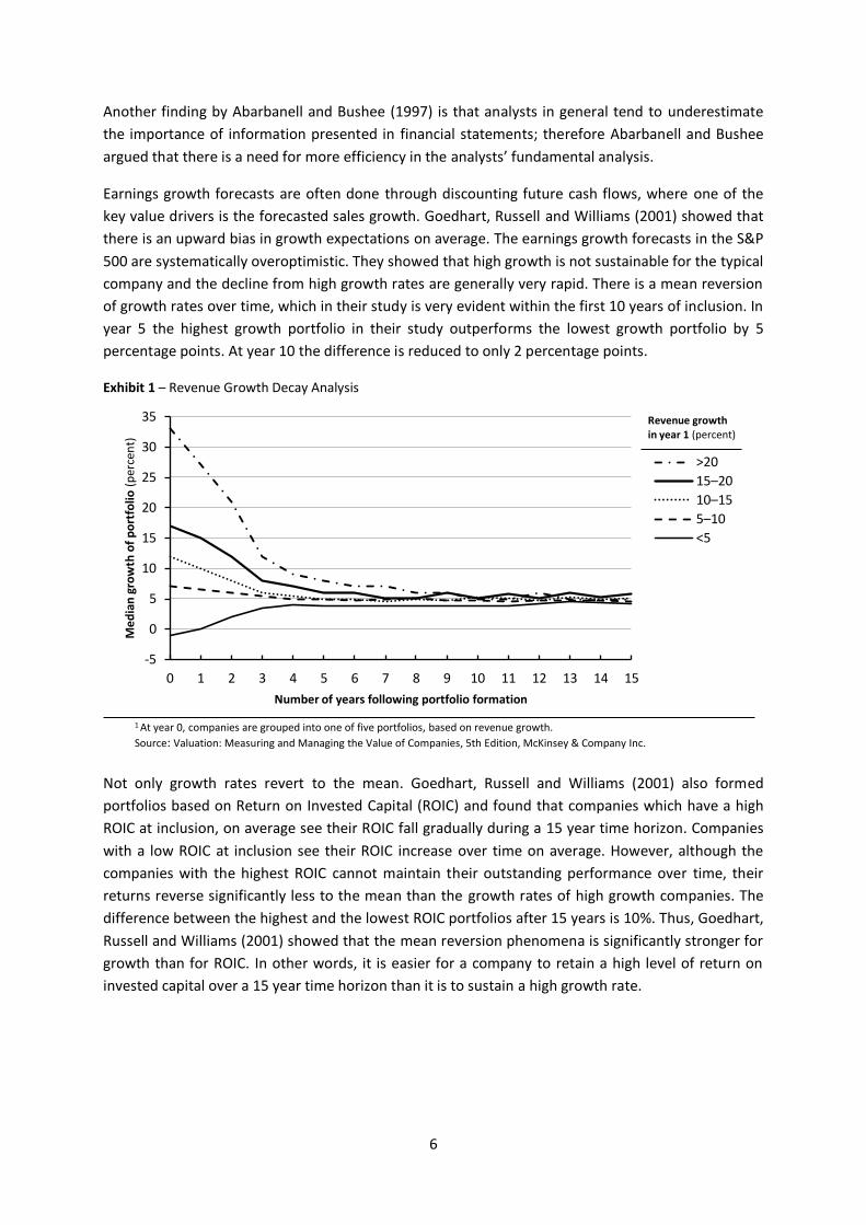
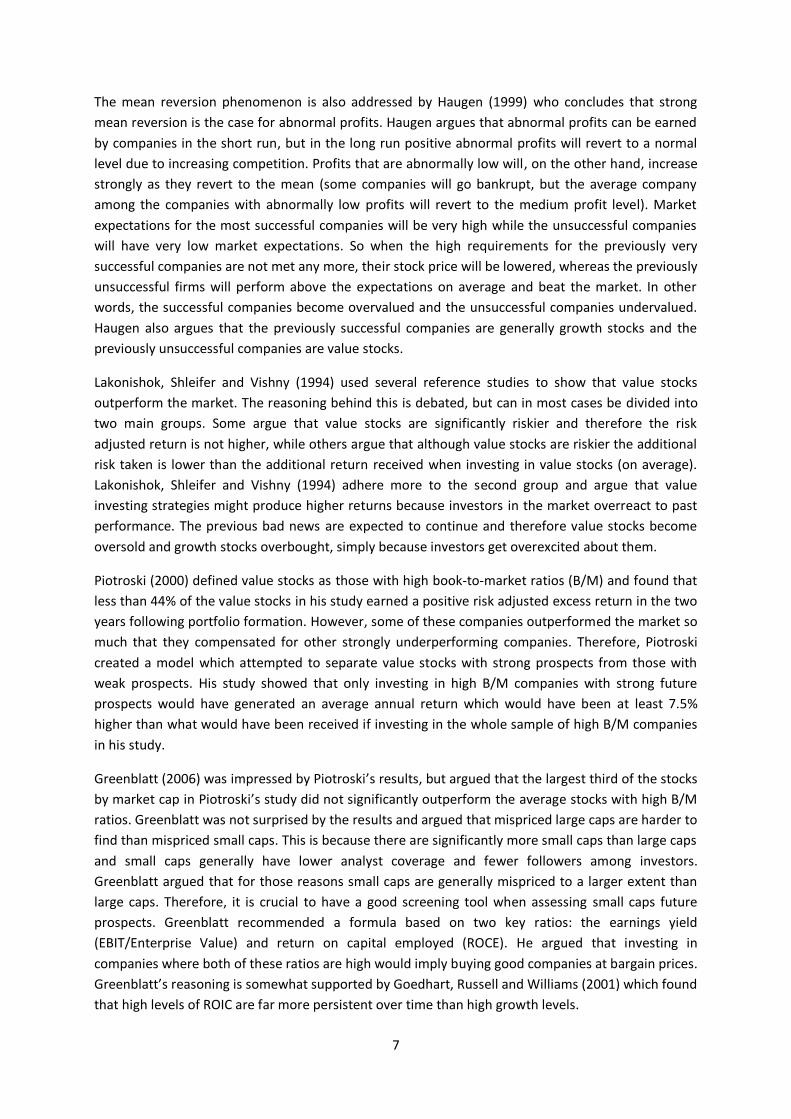
Earnings growth forecasts are often done through discounting future cash flows, where one of the

key value drivers is the forecasted sales growth. Goedhart, Russell and Williams (2001) showed that

there is an upward bias in growth expectations on average. The earnings growth forecasts in the S&P

500 are systematically overoptimistic. They showed that high growth is not sustainable for the typical

company and the decline from high growth rates are generally very rapid. There is a mean reversion

of growth rates over time, which in their study is very evident within the first 10 years of inclusion. In

year 5 the highest growth portfolio in their study outperforms the lowest growth portfolio by 5

percentage points. At year 10 the difference is reduced to only 2 percentage points.

Exhibit 1 – Revenue Growth Decay Analysis

Not only growth rates revert to the mean. Goedhart, Russell and Williams (2001) also formed

portfolios based on Return on Invested Capital (ROIC) and found that companies which have a high

ROIC at inclusion, on average see their ROIC fall gradually during a 15 year time horizon. Companies

with a low ROIC at inclusion see their ROIC increase over time on average. However, although the

companies with the highest ROIC cannot maintain their outstanding performance over time, their

returns reverse significantly less to the mean than the growth rates of high growth companies. The

difference between the highest and the lowest ROIC portfolios after 15 years is 10%. Thus, Goedhart,

Russell and Williams (2001) showed that the mean reversion phenomena is significantly stronger for

growth than for ROIC. In other words, it is easier for a company to retain a high level of return on

invested capital over a 15 year time horizon than it is to sustain a high growth rate.

-5

0

5

10

15

20

25

30

35

0 1 2 3 4 5 6 7 8 9 10 11 12 13 14 15

Me

dia

n g

row

th o

f p

ort

folio

(p

erce

nt)

Number of years following portfolio formation

>20

15–20

10–15

5–10

<5

Revenue growth in year 1 (percent)

1 At year 0, companies are grouped into one of five portfolios, based on revenue growth.

Source: Valuation: Measuring and Managing the Value of Companies, 5th Edition, McKinsey & Company Inc.

7

The mean reversion phenomenon is also addressed by Haugen (1999) who concludes that strong

mean reversion is the case for abnormal profits. Haugen argues that abnormal profits can be earned

by companies in the short run, but in the long run positive abnormal profits will revert to a normal

level due to increasing competition. Profits that are abnormally low will, on the other hand, increase

strongly as they revert to the mean (some companies will go bankrupt, but the average company

among the companies with abnormally low profits will revert to the medium profit level). Market

expectations for the most successful companies will be very high while the unsuccessful companies

will have very low market expectations. So when the high requirements for the previously very

successful companies are not met any more, their stock price will be lowered, whereas the previously

unsuccessful firms will perform above the expectations on average and beat the market. In other

words, the successful companies become overvalued and the unsuccessful companies undervalued.

Haugen also argues that the previously successful companies are generally growth stocks and the

previously unsuccessful companies are value stocks.

Lakonishok, Shleifer and Vishny (1994) used several reference studies to show that value stocks

outperform the market. The reasoning behind this is debated, but can in most cases be divided into

two main groups. Some argue that value stocks are significantly riskier and therefore the risk

adjusted return is not higher, while others argue that although value stocks are riskier the additional

risk taken is lower than the additional return received when investing in value stocks (on average).

Lakonishok, Shleifer and Vishny (1994) adhere more to the second group and argue that value

investing strategies might produce higher returns because investors in the market overreact to past

performance. The previous bad news are expected to continue and therefore value stocks become

oversold and growth stocks overbought, simply because investors get overexcited about them.

Piotroski (2000) defined value stocks as those with high book-to-market ratios (B/M) and found that

less than 44% of the value stocks in his study earned a positive risk adjusted excess return in the two

years following portfolio formation. However, some of these companies outperformed the market so

much that they compensated for other strongly underperforming companies. Therefore, Piotroski

created a model which attempted to separate value stocks with strong prospects from those with

weak prospects. His study showed that only investing in high B/M companies with strong future

prospects would have generated an average annual return which would have been at least 7.5%

higher than what would have been received if investing in the whole sample of high B/M companies

in his study.

Greenblatt (2006) was impressed by Piotroski’s results, but argued that the largest third of the stocks

by market cap in Piotroski’s study did not significantly outperform the average stocks with high B/M

ratios. Greenblatt was not surprised by the results and argued that mispriced large caps are harder to

find than mispriced small caps. This is because there are significantly more small caps than large caps

and small caps generally have lower analyst coverage and fewer followers among investors.

Greenblatt argued that for those reasons small caps are generally mispriced to a larger extent than

large caps. Therefore, it is crucial to have a good screening tool when assessing small caps future

prospects. Greenblatt recommended a formula based on two key ratios: the earnings yield

(EBIT/Enterprise Value) and return on capital employed (ROCE). He argued that investing in

companies where both of these ratios are high would imply buying good companies at bargain prices.

Greenblatt’s reasoning is somewhat supported by Goedhart, Russell and Williams (2001) which found

that high levels of ROIC are far more persistent over time than high growth levels.

8

Greenblatt wants to buy these persistently high performing companies at a low price and therefore

sets a high earnings yield criterion as well as a high return on capital criterion. His study is performed

on U.S. data between 1988 and 2004 and his fundamental investing formula averages a return of

30.8% per year while the S&P 500 averages 12.4% per year during the same time period.

Concluding Remarks on Portfolio Performance

Benjamin Graham was one of the pioneers in fundamental analysis. Many of the theories outlined by

him are still valid today and it would therefore be interesting to evaluate the performance of these

portfolio strategies during the last decades. We have therefore decided to pursue with a modified

version of the strategy for the Defensive Investor as outlined by Graham.

The portfolio performance part of the previous research section starts with Graham and ends with

Greenblatt, because of the intention to show which major contributions that have been made to this

topic in between these two. Greenblatt’s strategy is chosen as the other portfolio strategy. This is

partly because it becomes interesting to contrast one of the oldest strategies based on fundamental

analysis with one of the more recent ones, but more importantly because of the success that

Greenblatt’s strategy has had on the U.S. market. It therefore becomes interesting to test whether a

strong performance could have been obtained if the strategy had been adopted on the Nordic

market and during a partially different time period than in the original study by Greenblatt.

Benchmark Selection Treynor and Mazuy (1966) tested if the performance of 57 mutual funds could be explained by an

ability to successfully time the market. The model is often referred to as the Market Timing Model.

They used a quadratic regression to separate the fund managers’ ability to anticipate major turns in

the stock market from successfully selecting undervalued stocks. Their findings suggest that none of

these mutual funds were successful in timing the market during the studied time horizon. Instead

they argued that the alpha generated by skillful managers would primarily be due to a good ability to

identify undervalued stocks. This is also in line with Graham’s (1973) reasoning that an investor

attempting to find undervalued stocks would have significantly better prospects to consistently

outperform the market, than those investors seeking to do so only by trying to time the market.

Jensen (1968) introduced a model that is often referred to as Jensen’s Alpha, which incorporates an

alpha measure into the Capital Asset Pricing Model (CAPM). Alpha is defined as the risk-adjusted

excess return over the return predicted by CAPM. A portfolio that generates a positive alpha is seen

to provide a risk-adjusted return in excess of the market portfolio. Jensen’s Alpha became one of the

most frequently used measures in portfolio performance evaluation.

However, the Market Timing Model and Jensen’s Alpha both became criticized. Grinblatt (1992)

highlighted that it’s very important in portfolio performance evaluation that the portfolios’

performance is tested towards an efficient benchmark. The result of the performance evaluation

varies a lot depending on which benchmark is used. Grinblatt questioned the credibility of CAPM as a

benchmark model, arguing that it suffers from size and dividend yield biases. The critique against

CAPM is also a critique against Jensen’s Alpha since it is based on CAPM.

9

Grinblatt also argued that Jensen’s Alpha does not account for the excess returns generated by

managers with a timing ability. On the other hand, the previous research by Treynor and Mazuy

(1966) had shown that none of the fund managers in their study demonstrated a clear timing ability.

Even Grinblatt himself found that most funds fail to successfully time the market.

Ferson and Schadt (1996) constructed a conditional version of Treynor and Mazuy’s unconditional

regressions. They showed that a negative timing coefficient can occur in an unconditional model such

as Treynor and Mazuy’s, even if a manager follows a buy and hold strategy and consequently does

not even attempt to time the market. Therefore the model is specified incorrectly. For the

conditional model which is outlined by Ferson and Schadt, the findings suggest that the incorporation

of conditional information removes the evidence of negative timing coefficients. In other words,

Ferson and Schadt (1996) argue that Treynor and Mazuy’s Market Timing Model cannot be used as a

credible model for portfolio performance benchmarking.

Ferson and Schadt (1996) also questioned Jensen’s Alpha and argued that it is well documented that

the model faces severe problems when betas and expected returns vary a lot over time. They also

argue that it is problematic that portfolio performance studies evaluated against CAPM and Jensen’s

Alpha show that the alphas are negative to a much larger extent than they are positive. This is

unreasonable since the pursuit for alpha is a zero sum game. The average generated alpha at a given

market is zero and therefore the strong bias towards negative alphas is indicating one of many

limitations with Jensen’s Alpha as a model for portfolio performance benchmarking.

Ferson and Schadt (1996) argued that the issue of finding a reliable benchmark model for evaluating

portfolio performance remained unsolved after more than 30 years of continuous attempts to find

such a model. However, they did not address the three factor model introduced by Fama and French

in 1992. The Fama French 3 Factor Model originated from a critique against CAPM’s ability to predict

portfolio returns in an accurate manner.

Running regressions for the Fama French 3 Factor Model and CAPM, shows that CAPM has a very low

explanatory power for the distribution of risk premiums between 1970 and 2011. However, if CAPM

is extended with 2 additional factors, one for size differences and one for differences in Book-to-

Market level (B/M), then the risk premiums under this time period are significantly better explained.

Fama and French argued that firm size and differences in B/M levels are two important factors for

explaining differences in risk between different stocks.

The Fama French 3 Factor Model became a very popular model for benchmarking portfolio

performance. The critique against it is especially directed towards the theory behind it, which is the

Efficient Market Hypothesis (EMH). Therefore, many investigations have been performed both to test

whether a specific strategy or equity fund has created a risk adjusted excess return, but also as a way

of questioning the Efficient Market Hypothesis.

10

Concluding Remarks on Benchmark Selection

We argue that the Efficient Market Hypothesis has suffered from much stronger critique than the

Fama French 3 Factor Model has as a benchmark model. However, a valid point is that a model loses

credibility if the theory behind it loses credibility. We therefore argue that there is a need for a more

academically valid model for risk-adjusted performance benchmarking, but in absence of better

alternatives, we have chosen to proceed with the Fama French 3 Factor Model as our choice of

academic benchmark model. We find that the Jensen’s Alpha model and the Market Timing Model by

Treynor and Mazuy have suffered too severe critique to be adequately credible as benchmark

models for portfolio performance evaluation. In addition, we have also chosen to use a practical

index called the FTSE Nordic 30 to serve as an additional benchmark.

11

Theoretical Framework and Method

Graham’s Investment Strategy One of the core learning points that Graham wanted to communicate is to look for companies with

large discrepancies between price and value.4 Generally the starting point is to estimate the value of

a specific company under normal economic conditions. This can be done in several ways, but Graham

thought it was important to emphasize that the choice of investment approach should depend on the

characteristics of the investor. Graham separated investors in two main groups: the Enterprising

Investor and the Defensive Investor. The Enterprising Investors are defined as those “willing to

continually research, select and monitor a dynamic mix of stocks, bonds and mutual funds”. The

Defensive Investors are basically all other investors.

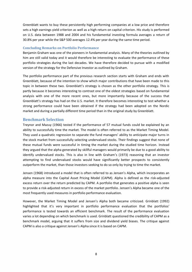
Graham outlined a strategy for stock selection, which he recommends the Defensive Investor to

pursue. The strategy includes seven criteria and the portfolio is recommended to be rebalanced

yearly. The original criteria as outlined by Graham are presented in Exhibit 2 along with the

modification of these criteria used in this study.

Exhibit 2 – The Original and Modified criteria of Graham’s investment strategy for the Defensive Investor

Graham’s Original Criteria5 Modified Criteria used in this study6

1. Sales ≥ USD 100 million 1. Sales ≥ SEK 1 billion

2. Current Ratio ≥ 2 2. Current Ratio ≥ 1.5

3. Long-Term Debt ≤ Net Working Capital 3. Long-Term Debt ≤ Net Working Capital

4. Positive Earnings for the last 10 years 4. Positive Earnings for the last 8 years

5. Uninterrupted Dividend payments for the last 20 years

5. Uninterrupted Dividend payments for the last 8 years

6. Cumulative Earnings Growth ≥ 33% over the last 10 years

6. Cumulative Earnings Growth ≥ 33% over the last 8 years

7. Current price should not exceed 15 times average earnings of the past three years

7. Select the 20 companies with the lowest P/E ratio which satisfy all other requirements

Graham wanted to provide the Defensive Investor with a model for stock selection that provided

safety but yet generated excess returns. The smallest companies are excluded in Graham’s model,

which is one way of lowering the risk. This is both done through setting a minimum sales

requirement, but also indirectly through setting a requirement for uninterrupted dividend payments

during the past 20 years, since a company that has managed to pay out dividends for 20 consecutive

years has generally grown relatively large. The model also excludes companies in a weak financial

position through setting a relatively high current ratio requirement and requiring that long-term debt

does not exceed net working capital. The earnings requirement excludes loss making companies and

prioritizes companies with stable earnings. The dividend requirement is also a criterion that indicates

a relatively stable performance of a business over time. The growth requirement is rather low, since

it implies an average annual earnings growth of approximately 3%.

4 Graham, B. (1973). The Intelligent Investor (4

th ed., 2003), Preface by Warren E. Buffett (page viii)

5 Graham also suggested an additional requirement of a maximum Price/Assets ratio of 1.5 or a combined criterion, where

the P/E ratio times the Price/Assets ratio is not higher than 22.5 6 The reasoning behind the modifications is discussed on pages 11-12

12

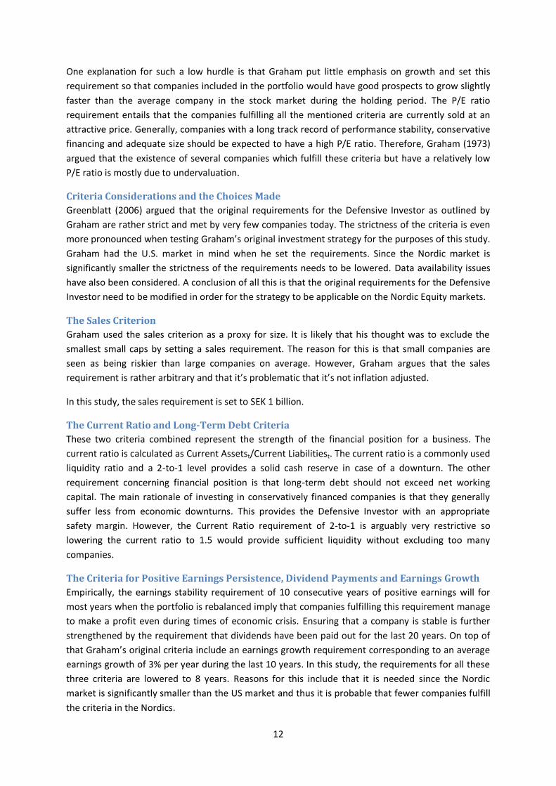
One explanation for such a low hurdle is that Graham put little emphasis on growth and set this

requirement so that companies included in the portfolio would have good prospects to grow slightly

faster than the average company in the stock market during the holding period. The P/E ratio

requirement entails that the companies fulfilling all the mentioned criteria are currently sold at an

attractive price. Generally, companies with a long track record of performance stability, conservative

financing and adequate size should be expected to have a high P/E ratio. Therefore, Graham (1973)

argued that the existence of several companies which fulfill these criteria but have a relatively low

P/E ratio is mostly due to undervaluation.

Criteria Considerations and the Choices Made

Greenblatt (2006) argued that the original requirements for the Defensive Investor as outlined by

Graham are rather strict and met by very few companies today. The strictness of the criteria is even

more pronounced when testing Graham’s original investment strategy for the purposes of this study.

Graham had the U.S. market in mind when he set the requirements. Since the Nordic market is

significantly smaller the strictness of the requirements needs to be lowered. Data availability issues

have also been considered. A conclusion of all this is that the original requirements for the Defensive

Investor need to be modified in order for the strategy to be applicable on the Nordic Equity markets.

The Sales Criterion

Graham used the sales criterion as a proxy for size. It is likely that his thought was to exclude the

smallest small caps by setting a sales requirement. The reason for this is that small companies are

seen as being riskier than large companies on average. However, Graham argues that the sales

requirement is rather arbitrary and that it’s problematic that it’s not inflation adjusted.

In this study, the sales requirement is set to SEK 1 billion.

The Current Ratio and Long-Term Debt Criteria

These two criteria combined represent the strength of the financial position for a business. The

current ratio is calculated as Current Assetst/Current Liabilitiest. The current ratio is a commonly used

liquidity ratio and a 2-to-1 level provides a solid cash reserve in case of a downturn. The other

requirement concerning financial position is that long-term debt should not exceed net working

capital. The main rationale of investing in conservatively financed companies is that they generally

suffer less from economic downturns. This provides the Defensive Investor with an appropriate

safety margin. However, the Current Ratio requirement of 2-to-1 is arguably very restrictive so

lowering the current ratio to 1.5 would provide sufficient liquidity without excluding too many

companies.

The Criteria for Positive Earnings Persistence, Dividend Payments and Earnings Growth

Empirically, the earnings stability requirement of 10 consecutive years of positive earnings will for

most years when the portfolio is rebalanced imply that companies fulfilling this requirement manage

to make a profit even during times of economic crisis. Ensuring that a company is stable is further

strengthened by the requirement that dividends have been paid out for the last 20 years. On top of

that Graham’s original criteria include an earnings growth requirement corresponding to an average

earnings growth of 3% per year during the last 10 years. In this study, the requirements for all these

three criteria are lowered to 8 years. Reasons for this include that it is needed since the Nordic

market is significantly smaller than the US market and thus it is probable that fewer companies fulfill

the criteria in the Nordics.

13

Another reason is that the original requirement that a company must have been paying out dividends

for the past 20 years, implies that several companies will be excluded simply because they have not

existed for 20 years. In addition to that, many companies do not even start to pay out dividends

regularly before the early years of the company is over. Therefore it is arguably unnecessary to

require that dividends are paid out for 20 consecutive years. Also lowering the growth horizon to 8

years but keeping the request for a cumulative growth of 33% over these years implies requesting a

higher growth rate per year, but during a shorter time period than Graham’s original requirements.

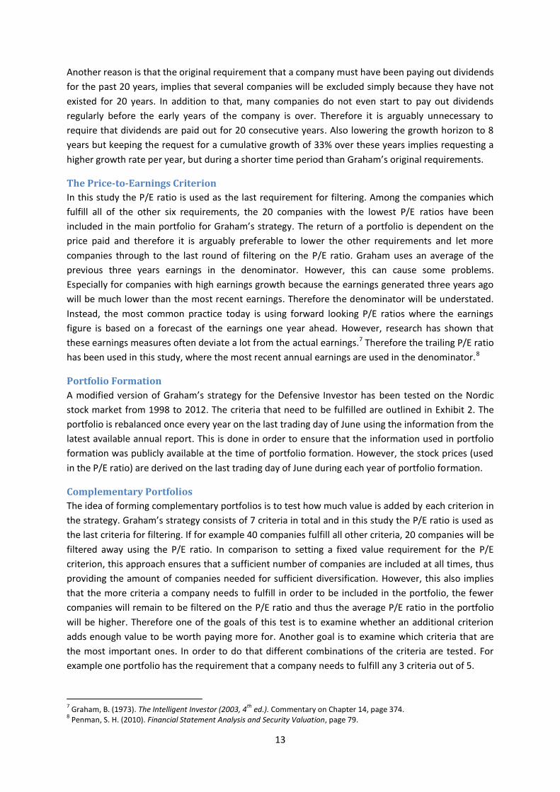
The Price-to-Earnings Criterion

In this study the P/E ratio is used as the last requirement for filtering. Among the companies which

fulfill all of the other six requirements, the 20 companies with the lowest P/E ratios have been

included in the main portfolio for Graham’s strategy. The return of a portfolio is dependent on the

price paid and therefore it is arguably preferable to lower the other requirements and let more

companies through to the last round of filtering on the P/E ratio. Graham uses an average of the

previous three years earnings in the denominator. However, this can cause some problems.

Especially for companies with high earnings growth because the earnings generated three years ago

will be much lower than the most recent earnings. Therefore the denominator will be understated.

Instead, the most common practice today is using forward looking P/E ratios where the earnings

figure is based on a forecast of the earnings one year ahead. However, research has shown that

these earnings measures often deviate a lot from the actual earnings.7 Therefore the trailing P/E ratio

has been used in this study, where the most recent annual earnings are used in the denominator.8

Portfolio Formation

A modified version of Graham’s strategy for the Defensive Investor has been tested on the Nordic

stock market from 1998 to 2012. The criteria that need to be fulfilled are outlined in Exhibit 2. The

portfolio is rebalanced once every year on the last trading day of June using the information from the

latest available annual report. This is done in order to ensure that the information used in portfolio

formation was publicly available at the time of portfolio formation. However, the stock prices (used

in the P/E ratio) are derived on the last trading day of June during each year of portfolio formation.

Complementary Portfolios

The idea of forming complementary portfolios is to test how much value is added by each criterion in

the strategy. Graham’s strategy consists of 7 criteria in total and in this study the P/E ratio is used as

the last criteria for filtering. If for example 40 companies fulfill all other criteria, 20 companies will be

filtered away using the P/E ratio. In comparison to setting a fixed value requirement for the P/E

criterion, this approach ensures that a sufficient number of companies are included at all times, thus

providing the amount of companies needed for sufficient diversification. However, this also implies

that the more criteria a company needs to fulfill in order to be included in the portfolio, the fewer

companies will remain to be filtered on the P/E ratio and thus the average P/E ratio in the portfolio

will be higher. Therefore one of the goals of this test is to examine whether an additional criterion

adds enough value to be worth paying more for. Another goal is to examine which criteria that are

the most important ones. In order to do that different combinations of the criteria are tested. For

example one portfolio has the requirement that a company needs to fulfill any 3 criteria out of 5.

7 Graham, B. (1973). The Intelligent Investor (2003, 4

th ed.). Commentary on Chapter 14, page 374.

8 Penman, S. H. (2010). Financial Statement Analysis and Security Valuation, page 79.

14

These 5 criteria are the requirements for: Current Ratio, Long-Term Debt, Positive Earnings

Persistence, Dividend Payments Persistence and Earnings Growth. The sales requirement (which is

used as a size indicator) is included in the main portfolio, but is not included in any of the

complementary portfolios. One reason for this is that the sales requirement is so low that very few

companies are filtered away because of it. Another reason is that several empirical researches have

shown that the average return for small companies is higher than for large companies and therefore

the results should not be improved by setting a size requirement.9 The sales requirement is used

instead of using market cap as the size requirement because this makes the strategy more

comparable to Graham’s original strategy.

Greenblatt’s Investment Strategy Benjamin Graham is repeatedly referred to in Greenblatt’s book: ”The Little Book that Beats the

Market”. Greenblatt adheres to Graham’s argument that an investor should strive to buy companies

which are traded at large discounts in relation to their fair values, thus providing a “margin of safety”

as well as a higher probability of obtaining excess returns. He also argues that the fair values of most

listed companies move relatively little from one year to another, while the prices of the same

companies fluctuate a lot on average.10 In the long run however, the prices will equal the fair values

and thus an investor can benefit from buying stocks at prices significantly lower than their fair value

during normal economic conditions.11 Both Greenblatt and Graham advocate patience in investing

and that it can take several years before their respective strategies pay off as intended to.

Although Greenblatt’s strategy relies on many of the core theories developed by Graham, Greenblatt

argues that the original requirements included in the strategy for the Defensive Investor, are very

strict and only met by very few listed companies in today’s markets. A large part of Graham’s success

was obtained during the Great Depression and throughout the Second World War, times when the

stock market was perceived as very risky. Because of this, many stocks were priced cheaply.12

Greenblatt argues that his strategy has less strict requirements than Graham’s; it is more flexible and

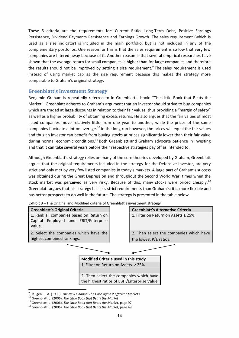
has better prospects to do well in the future. The strategy is presented in the table below.

Exhibit 3 – The Original and Modified criteria of Greenblatt’s investment strategy

Greenblatt’s Original Criteria Greenblatt’s Alternative Criteria 1. Rank all companies based on Return on Capital Employed and EBIT/Enterprise Value.

1. Filter on Return on Assets ≥ 25%.

2. Select the companies which have the highest combined rankings.

2. Then select the companies which have

the lowest P/E ratios.

ratio

Modified Criteria used in this study

1. Filter on Return on Assets ≥ 25%

2. Then select the companies which have the highest ratios of EBIT/Enterprise Value

9 Haugen, R. A. (1999). The New Finance: The Case Against Efficient Markets.

10 Greenblatt, J. (2006). The Little Book that Beats the Market

11 Greenblatt, J. (2006). The Little Book that Beats the Market, page 97

12 Greenblatt, J. (2006). The Little Book that Beats the Market, page 49

15

Greenblatt’s strategy involves investing in companies which have a high return on capital and a high

earnings yield. In short, this is described as “buying high performing companies at bargain prices”.13

In a large sample of companies this will imply “buying companies performing well above average at

prices well below average”, according to Greenblatt (2006). In his study, Greenblatt demonstrates

that the combination of the two criteria has led to an impressing average annual return of 30.8% per

year from 1988 to 2004. The average annual return for the S&P 500 during the corresponding period

was 12.4%. The entire portfolio consisted of stocks trading at the U.S. stock market. The portfolio

was rebalanced once a year and consisted of 30 stocks during the entire time period.

The Return on Capital Criterion

Generally, a high return on capital for example measured as ROCE, ROA, ROE or ROIC, is an indication

that a company has a strong competitive advantage.14 This is especially true if the high return on

capital has been persistent during several consecutive years. Greenblatt (2006) argues that

companies which generate high returns, generally also have better prospects to reinvest their profits

in projects which will generate high returns. This is also supported by Goedhart, Russell and Williams

(2001) who have shown that high levels of ROIC are rather persistent over time.15

Greenblatt favored using Return on Capital Employed (ROCE) as the capital requirement.16 As an

alternative he recommends using Return on Assets (ROA) instead of ROCE.17 The reason for using

ROA instead of ROCE in this study is because of significantly better data availability for ROA among

the publicly listed Nordic companies during the tested time period. ROA is calculated using EBIT as

the earnings measure, which benefits from being calculated before taxes and interest expenses. This

enables a comparison between companies with different debt levels and tax rates. It could also be

argued that it is more interesting to see which earnings that are generated from operating activities

rather than a mix of operating activities, financial and tax deduction activities. It is also important to

note that the different Nordic countries have different tax rates and tax policies; in addition to that

many companies generate their earnings in several different countries and are thus affected by their

tax rules. Therefore EBIT is a very appropriate earnings measure.

The Earnings Yield Criterion

Filtering companies on a high EBIT/Enterprise Value is chosen instead of filtering on low P/E ratios.18

One of the reasons for this is that the earnings measure in the P/E ratio is generally calculated after

tax and as explained earlier it is preferable to use an earnings measure which is calculated before tax

and interest expenses for comparability reasons. A reason for using Enterprise Value instead of only

the market value of equity is because the operating earnings are generated by assets financed by

both equity and debt. Another reason is that using Enterprise Value enhances comparability between

companies with different levels of debt financing.

13

Greenblatt, J. (2006). The Little Book that Beats the Market, page 45 14

Greenblatt, J. (2006). The Little Book that Beats the Market, page 85 15

Goedhart, Russell & Williams (2001). Prophets and Profits. McKinsey on Finance, No.2 16

ROCE is defined as: 17

ROA is defined as: 18

Enterprise value is defined as Market Value of Equity + Interest-bearing Net Debt.

16

A high operating earnings yield is an indication that a company earns a lot in comparison to the

purchase price of the business. It can also indicate that the company has a justified debt level and

that it is trading at a low price.

Portfolio Formation

A modified version of Greenblatt’s strategy is tested on the Nordic stock market between 1998 and

2012. The criteria that need to be fulfilled are outlined in Exhibit 3. The portfolio is rebalanced once

every year on the last trading day of June. In accordance with Greenblatt’s recommendations, the

standard ROA requirement is set to only include companies which have a ROA of at least 25%.19 This

is the first requirement that a company needs to pass in order to be considered for inclusion in the

portfolio. After meeting the ROA requirement the 20 companies which have the highest earnings

yield are selected.

Complementary Portfolios

Similarly to the complementary portfolios for Graham’s strategy, those for Greenblatt are

constructed with the purpose of testing the importance each criterion has in generating the returns.

The complementary portfolios for Greenblatt are however structured differently than those for

Graham. Each year, the publicly listed stocks on the Nordic market are separated into four different

groups based on their level of ROA. These portfolios are therefore called Quartile portfolios. The 1st

quartile includes the companies with the highest ROA level and the 4th quartile the companies with

the lowest ROA level. Since the Greenblatt strategy consists of two criteria, ROA and Earnings yield,

all 4 quartile portfolios are divided into high and low yield portfolios. Thus the 1st Quartile Portfolio is

divided into one portfolio including the companies with the highest earnings yield (and the highest

ROA level) and another portfolio with the companies with the lowest earnings yield (but with the

highest ROA level). This results in 8 complementary portfolios. The portfolio called 1st Quartile High

Earnings Yield is rather similar to the Greenblatt standard portfolio, with the difference that the

Standard Portfolio contains fewer stocks and consequently has a higher average ROA and a higher

average earnings yield.

However, there are some companies which manage to achieve a ROA level of at least 25% during

several consecutive years. Therefore it is reasonable to believe that these companies are worth

paying more for (here indicated by a lower earnings yield), since these companies have a momentum

of high performance. Therefore an additional complementary portfolio has been constructed which

primarily involves investing in companies which have had a ROA level of at least 25% during at least

two consecutive years. If less than 20 companies fulfill these criteria, then the rest of the companies

which are included have to fulfill the standard requirements only. An important distinction between

this portfolio and the other portfolios based on Greenblatt’s strategy is that in this portfolio

preference is given to the ROA criterion at the expense of high earnings yields. Therefore the

portfolio is called Greenblatt Momentum Preference.

19

Except for the portfolio formed in 2003, during which the ROA requirement was lowered to 22% because of significantly fewer companies managing to satisfy the standard threshold of 25%.

17

The Fama French Three Factor Model When evaluating the performance of an investment strategy, the return generated from the strategy

should be set in relation to an appropriate benchmark. A statistically significant alpha generated in

the regression would indicate that a strategy is capable of generating a return which cannot be easily

captured by conventional models. The benchmark model used in this study is the Fama French 3

Factor Model.

The reasons for choosing this model have been discussed in the Previous Research section.

Empirically the Fama French 3 Factor Model manages to capture the stock performance much better

than CAPM for example. For this reason the Fama French 3 Factor Model is frequently used in

contemporary academic research and has been referred to as a “cornerstone of empirical financial

research”.20 The equation for the model is:

Rp,t is the return of a tested portfolio during a specific time period. The returns and the risk free rate

Rf,t are calculated on a monthly basis. Swedish 6 month government bond rates are used as the risk

free rate. Alpha (αp) is the risk adjusted excess return generated from the tested portfolios. An

accumulated alpha which is positive and significant indicates that a tested portfolio generates an

excess return adjusted for market, size and value factors, which according to Fama and French are

associated with a higher risk. Alpha is calculated as the residual in this model. Beta (Mkt) sets the

volatility of a tested portfolio in relation to the market portfolio. The return of the market portfolio is

calculated as a value-weighted return based on all publicly listed companies in the Nordics.

SMB stands for Small minus Big and is calculated by subtracting the average return generated from

the largest stocks from that of the smallest stocks. All companies listed at the Nordic market are

sorted on market capitalization and the 25% which has the highest market cap are included among

the large companies. The average return from these companies is subtracted from the average

return of the remaining companies which correspond to 75% of the market. The SMB portfolio is

value weighted and constructed on the last trading day of June each year. The portfolio formation

procedure is in accordance with the one employed by Fama and French (1993) in their original

study.21

HML stands for High minus Low which is calculated through subtracting the monthly returns of the

companies with the lowest Book-to-Market ratios from the companies with the highest Book-to-

Market ratios. All listed companies in the Nordic market are ranked on their B/M ratios. The returns

for the 30% of stocks which have the lowest B/M ratios are subtracted from the returns for the 30%

of stocks with the highest B/M ratios. The portfolio is rebalanced each year on the last trading day in

June, although the book value is extracted from the latest annual report. The returns are value-

weighted and the procedure is in accordance with the original study by Fama and French (1993).

20

Chan, L. K. C., Dimmock, S. G., Lakonishok, J. (2006). Benchmarking Money Manager Performance: Issues and Evidence 21

The exact construction procedure is slightly different as Fama and French used U.S. data originating from 3 different stock exchanges (NYSE, AMEX and NASDAQ). Nevertheless, the resulting portfolio characteristics are closely matching those achieved by Fama and French.

18

Return Measurements

A monthly total return index is used to measure the returns of all the individual stocks and

consequently for all the portfolios and benchmarks. A total return means that the return includes

both movements in stock price and dividends paid out during the period. The dividends are

continuously reinvested in the stocks they have been generated from. This is done in order to ensure

that the results are relevant for investors.

Time Period Considerations

Thomson Reuters Datastream is a database which commenced an extensive coverage of European

markets in 1988 after opening a data processing center in Ireland. Therefore the availability of

financial accounting data for publicly listed Nordic companies significantly improves from 1988 and

onwards. This also implies that variables calculated before 1988 might be expressed in a different

format, which is the case for the Total Return Index. This index used to treat dividends differently

before 1988. For this reason, extending the research period to include data before 1988 would make

this study more prone to data errors in the results and decrease comparability. As some of Graham’s

criteria require a pre-investment horizon of 10 years, data availability considerations make 1998 the

first investment year in this study.

The Nordic Market The Nordic stock market consists of companies listed in Sweden, Norway, Denmark, Finland and

Iceland. All countries are small open economies which are rather reliant on foreign trade. The largest

part of the export is to countries in Western Europe and the U.S. This has implied that the region is

sensitive to global economic cycles, for example the region has suffered extensively from the latest

financial crisis.22

Historically the region has invested considerable amounts in public welfare including infrastructure,

education and science.23 This has facilitated the economic development which involves successfully

monetizing on both the natural resources in the region, as well as creating a strong service oriented

society. All of this has contributed to the fact that the Nordic region is one of the richest regions in

the world with numerous large international companies.24 25

Main Industries

Overall the region has been monetizing on natural resources such as forestry, mining, fishing and

food products. Norway has also been successfully monetizing on their extensive oil resources. In

addition to that, many companies are involved in businesses related to machinery and electronic

equipment. However, many of the fastest growing businesses are service oriented; this has especially

been the case for Sweden and Finland during the tested time horizon.26 Both countries have a large

exposure to the information and communications industry.27

22

Norden.org 23

Norden.org 24

Forbes.com – The World’s Biggest Public Companies 25

CIA.gov – The World Factbook 26

Indexmundi.com – Swedish GDP by Sector 27

CIA.gov – The World Factbook

19

Dominating Companies

In 2011, Statoil’s revenues accounted for 24% of Norway’s GDP and Nokia’s revenues accounted for

20% of Finland’s GDP. Therefore, the movements on the Norwegian and Finish markets have been

strongly affected by two companies during the studied time period. These companies can therefore

have a large explanatory power for short term fluctuations on these markets. However, investing in

the Nordic market implies significantly lower weights for large companies such as Statoil and Nokia

than investing in only the Norwegian or the Finish market. Their size in relation to the entire Nordic

stock market in terms of market capitalization corresponded to 8.34% for Statoil and 1.85% for Nokia

in December 2011. In this study, it has been tested to set a market cap limit, so that no company has

a larger market cap then 5% of the market. However, the impact on the results generated by setting

this market cap limit was low.

These results imply that the Nordic region as a whole provides good diversification opportunities in a

sense that none of the countries does on a standalone basis. Finding high performing companies in

accordance with Graham’s and Greenblatt’s criteria were harder during the worst years of the IT

boom, but it would have been a lot worse if investments had only been made in one of the countries’

stock markets.

20

Results and Analysis Some of the results in this study were at first rather unexpected, because the two best performing

portfolios were not among the two main portfolios. Instead the best performing portfolios were

found when sensitivity testing Graham’s strategy for the Defensive Investor. As it later turned out,

Graham also appears to have made the same findings and he suggested a new strategy based on

them. The results in this section are presented in the order they were discovered. Following this story

facilitates the understanding of the rationale behind the results and the derivation of them.

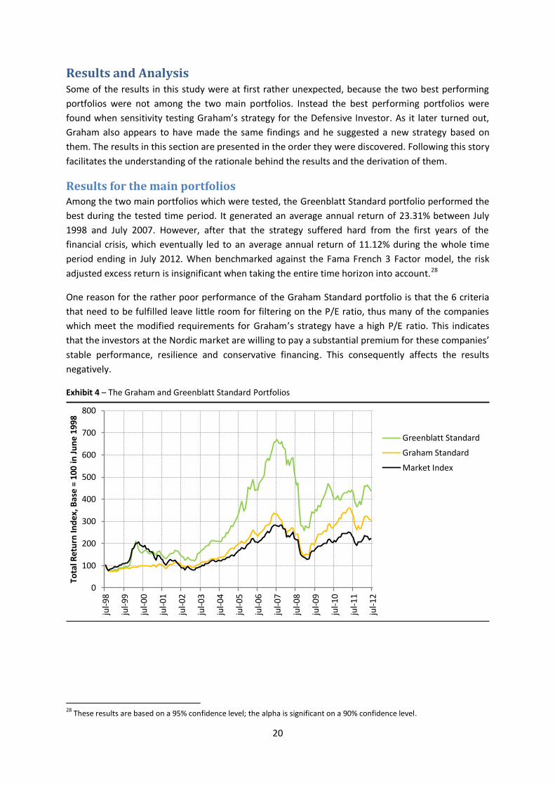
Results for the main portfolios Among the two main portfolios which were tested, the Greenblatt Standard portfolio performed the

best during the tested time period. It generated an average annual return of 23.31% between July

1998 and July 2007. However, after that the strategy suffered hard from the first years of the

financial crisis, which eventually led to an average annual return of 11.12% during the whole time

period ending in July 2012. When benchmarked against the Fama French 3 Factor model, the risk

adjusted excess return is insignificant when taking the entire time horizon into account.28

One reason for the rather poor performance of the Graham Standard portfolio is that the 6 criteria

that need to be fulfilled leave little room for filtering on the P/E ratio, thus many of the companies

which meet the modified requirements for Graham’s strategy have a high P/E ratio. This indicates

that the investors at the Nordic market are willing to pay a substantial premium for these companies’

stable performance, resilience and conservative financing. This consequently affects the results

negatively.

Exhibit 4 – The Graham and Greenblatt Standard Portfolios

28

These results are based on a 95% confidence level; the alpha is significant on a 90% confidence level.

0

100

200

300

400

500

600

700

800

jul-

98

jul-

99

jul-

00

jul-

01

jul-

02

jul-

03

jul-

04

jul-

05

jul-

06

jul-

07

jul-

08

jul-

09

jul-

10

jul-

11

jul-

12

Tota

l Ret

urn

Ind

ex, B

ase

= 1

00 in

Ju

ne

1998

Greenblatt Standard

Graham Standard

Market Index

21

Results for Greenblatt’s complementary portfolios

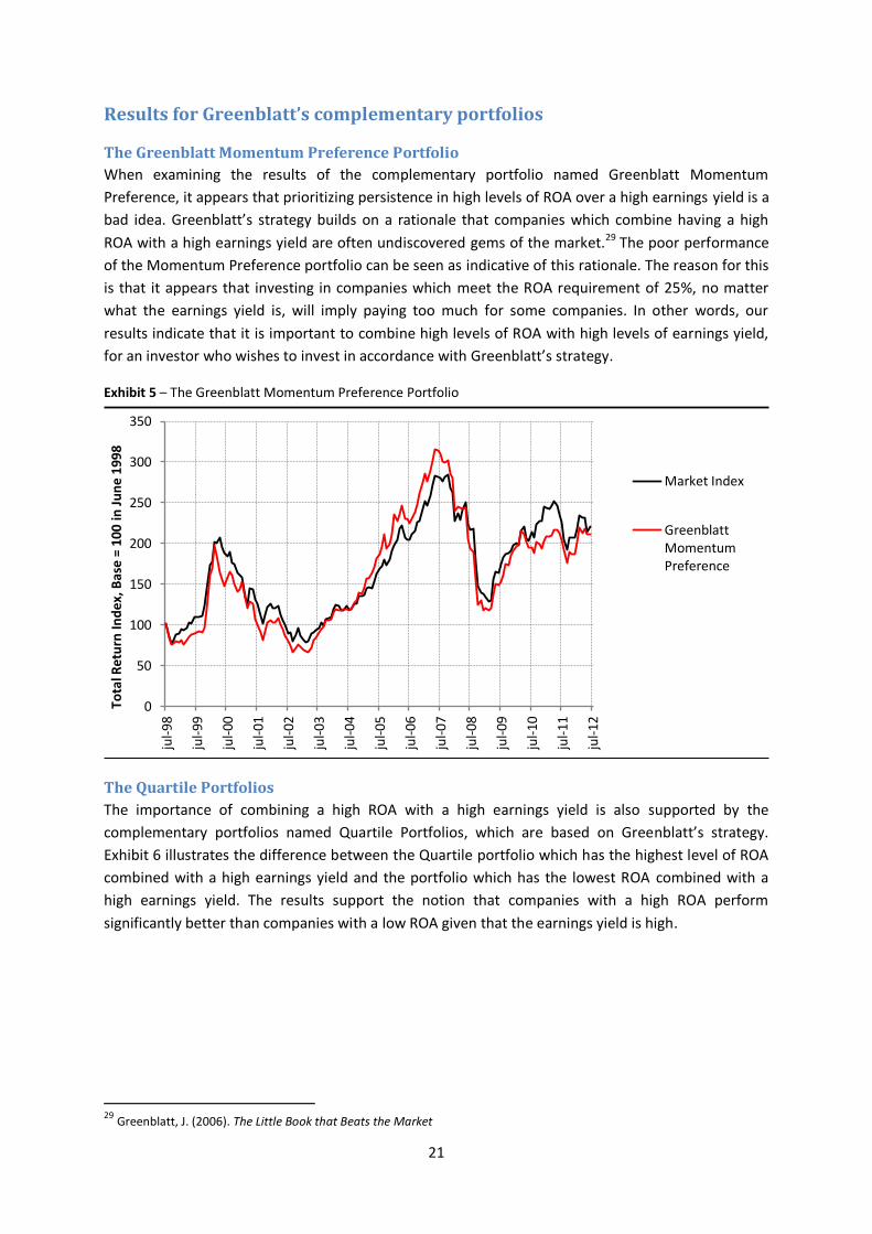
The Greenblatt Momentum Preference Portfolio

When examining the results of the complementary portfolio named Greenblatt Momentum

Preference, it appears that prioritizing persistence in high levels of ROA over a high earnings yield is a

bad idea. Greenblatt’s strategy builds on a rationale that companies which combine having a high

ROA with a high earnings yield are often undiscovered gems of the market.29 The poor performance

of the Momentum Preference portfolio can be seen as indicative of this rationale. The reason for this

is that it appears that investing in companies which meet the ROA requirement of 25%, no matter

what the earnings yield is, will imply paying too much for some companies. In other words, our

results indicate that it is important to combine high levels of ROA with high levels of earnings yield,

for an investor who wishes to invest in accordance with Greenblatt’s strategy.

Exhibit 5 – The Greenblatt Momentum Preference Portfolio

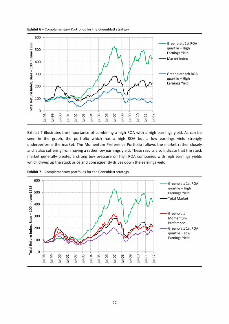
The Quartile Portfolios

The importance of combining a high ROA with a high earnings yield is also supported by the

complementary portfolios named Quartile Portfolios, which are based on Greenblatt’s strategy.

Exhibit 6 illustrates the difference between the Quartile portfolio which has the highest level of ROA

combined with a high earnings yield and the portfolio which has the lowest ROA combined with a

high earnings yield. The results support the notion that companies with a high ROA perform

significantly better than companies with a low ROA given that the earnings yield is high.

29 Greenblatt, J. (2006). The Little Book that Beats the Market

0

50

100

150

200

250

300

350

jul-

98

jul-

99

jul-

00

jul-

01

jul-

02

jul-

03

jul-

04

jul-

05

jul-

06

jul-

07

jul-

08

jul-

09

jul-

10

jul-

11

jul-

12

Tota

l Ret

urn

Ind

ex, B

ase

= 1

00 in

Ju

ne

1998

Market Index

Greenblatt Momentum Preference

22

Exhibit 6 – Complementary Portfolios for the Greenblatt strategy

Exhibit 7 illustrates the importance of combining a high ROA with a high earnings yield. As can be

seen in the graph, the portfolio which has a high ROA but a low earnings yield strongly

underperforms the market. The Momentum Preference Portfolio follows the market rather closely

and is also suffering from having a rather low earnings yield. These results also indicate that the stock

market generally creates a strong buy pressure on high ROA companies with high earnings yields

which drives up the stock price and consequently drives down the earnings yield.

Exhibit 7 – Complementary portfolios for the Greenblatt strategy

0

100

200

300

400

500

600

jul-

98

jul-

99

jul-

00

jul-

01

jul-

02

jul-

03

jul-

04

jul-

05

jul-

06

jul-

07

jul-

08

jul-

09

jul-

10

jul-

11

jul-

12 To

tal R

etu

rn In

dex

, Bas

e =

100

in J

un

e 19

98

Greenblatt 1st ROA quartile + High Earnings Yield

Market Index

Greenblatt 4th ROA quartile + High Earnings Yield

0

100

200

300

400

500

600

jul-

98

jul-

99

jul-

00

jul-

01

jul-

02

jul-

03

jul-

04

jul-

05

jul-

06

jul-

07

jul-

08

jul-

09

jul-

10

jul-

11

jul-

12 To

tal R

etu

rn In

dex

, Bas

e =

100

in J

un

e 19

98 Greenblatt 1st ROA

quartile + High Earnings Yield

Total Market

Greenblatt Momentum Preference

Greenblatt 1st ROA quartile + Low Earnings Yield

23

The cornerstone of value investing is buying companies which have a large discrepancy between

price and value.30 This reasoning is supported by the complementary portfolios connected to

Greenblatt’s strategy. The results imply that buying companies with a high ROA at high prices has not

been a good investment at the Nordic market during the time period of this study. The results are

vastly improved if an investor only buys high ROA companies at high earnings yields (indicating a low

price). Since the results show an indication of a relatively steep price increase in these companies, it

is also recommended to rebalance the portfolio at least once a year.

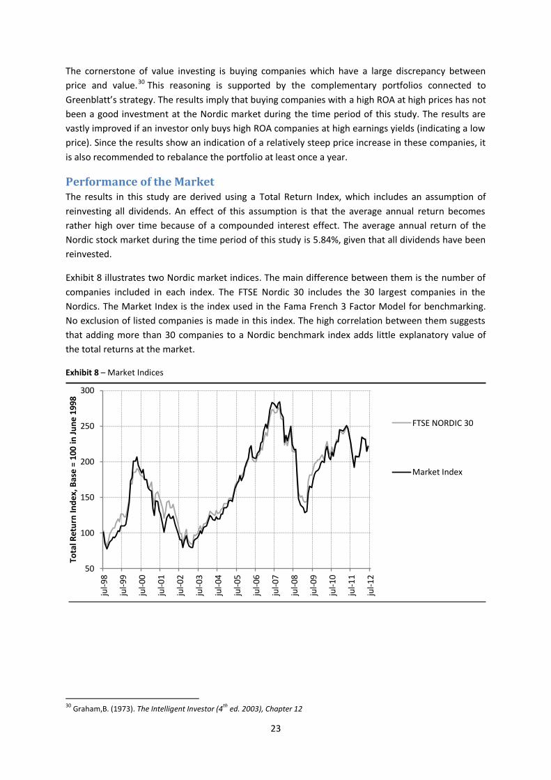
Performance of the Market The results in this study are derived using a Total Return Index, which includes an assumption of

reinvesting all dividends. An effect of this assumption is that the average annual return becomes

rather high over time because of a compounded interest effect. The average annual return of the

Nordic stock market during the time period of this study is 5.84%, given that all dividends have been

reinvested.

Exhibit 8 illustrates two Nordic market indices. The main difference between them is the number of

companies included in each index. The FTSE Nordic 30 includes the 30 largest companies in the

Nordics. The Market Index is the index used in the Fama French 3 Factor Model for benchmarking.

No exclusion of listed companies is made in this index. The high correlation between them suggests

that adding more than 30 companies to a Nordic benchmark index adds little explanatory value of

the total returns at the market.

Exhibit 8 – Market Indices

30

Graham,B. (1973). The Intelligent Investor (4th

ed. 2003), Chapter 12

50

100

150

200

250

300

jul-

98

jul-

99

jul-

00

jul-

01

jul-

02

jul-

03

jul-

04

jul-

05

jul-

06

jul-

07

jul-

08

jul-

09

jul-

10

jul-

11

jul-

12

Tota

l Ret

urn

Ind

ex, B

ase

= 1

00 in

Ju

ne

1998

FTSE NORDIC 30

Market Index

24

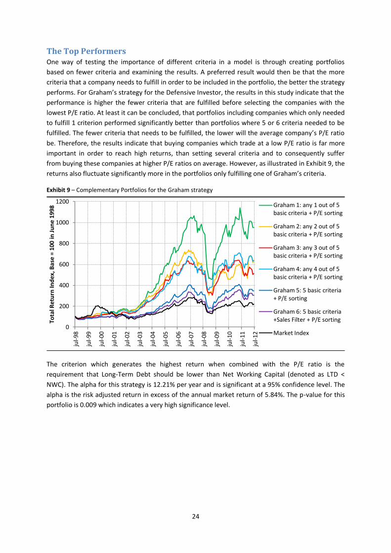
The Top Performers One way of testing the importance of different criteria in a model is through creating portfolios

based on fewer criteria and examining the results. A preferred result would then be that the more

criteria that a company needs to fulfill in order to be included in the portfolio, the better the strategy

performs. For Graham’s strategy for the Defensive Investor, the results in this study indicate that the

performance is higher the fewer criteria that are fulfilled before selecting the companies with the

lowest P/E ratio. At least it can be concluded, that portfolios including companies which only needed

to fulfill 1 criterion performed significantly better than portfolios where 5 or 6 criteria needed to be

fulfilled. The fewer criteria that needs to be fulfilled, the lower will the average company’s P/E ratio

be. Therefore, the results indicate that buying companies which trade at a low P/E ratio is far more

important in order to reach high returns, than setting several criteria and to consequently suffer

from buying these companies at higher P/E ratios on average. However, as illustrated in Exhibit 9, the

returns also fluctuate significantly more in the portfolios only fulfilling one of Graham’s criteria.

Exhibit 9 – Complementary Portfolios for the Graham strategy

The criterion which generates the highest return when combined with the P/E ratio is the

requirement that Long-Term Debt should be lower than Net Working Capital (denoted as LTD <

NWC). The alpha for this strategy is 12.21% per year and is significant at a 95% confidence level. The

alpha is the risk adjusted return in excess of the annual market return of 5.84%. The p-value for this

portfolio is 0.009 which indicates a very high significance level.

0

200

400

600

800

1000

1200

jul-

98

jul-

99

jul-

00

jul-

01

jul-

02

jul-

03

jul-

04

jul-

05

jul-

06

jul-

07

jul-

08

jul-

09

jul-

10

jul-

11

jul-

12

Tota

l Ret

urn

Ind

ex, B

ase

= 1

00 in

Ju

ne

1998

Graham 1: any 1 out of 5 basic criteria + P/E sorting

Graham 2: any 2 out of 5 basic criteria + P/E sorting

Graham 3: any 3 out of 5 basic criteria + P/E sorting

Graham 4: any 4 out of 5 basic criteria + P/E sorting

Graham 5: 5 basic criteria + P/E sorting

Graham 6: 5 basic criteria +Sales Filter + P/E sorting

Market Index

25

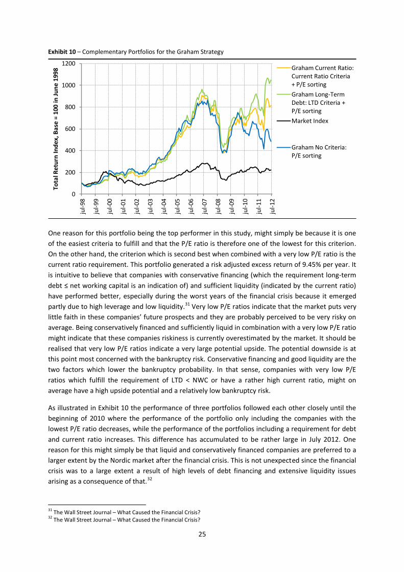
Exhibit 10 – Complementary Portfolios for the Graham Strategy

One reason for this portfolio being the top performer in this study, might simply be because it is one

of the easiest criteria to fulfill and that the P/E ratio is therefore one of the lowest for this criterion.

On the other hand, the criterion which is second best when combined with a very low P/E ratio is the

current ratio requirement. This portfolio generated a risk adjusted excess return of 9.45% per year. It

is intuitive to believe that companies with conservative financing (which the requirement long-term

debt ≤ net working capital is an indication of) and sufficient liquidity (indicated by the current ratio)

have performed better, especially during the worst years of the financial crisis because it emerged

partly due to high leverage and low liquidity.31 Very low P/E ratios indicate that the market puts very

little faith in these companies’ future prospects and they are probably perceived to be very risky on

average. Being conservatively financed and sufficiently liquid in combination with a very low P/E ratio

might indicate that these companies riskiness is currently overestimated by the market. It should be

realised that very low P/E ratios indicate a very large potential upside. The potential downside is at

this point most concerned with the bankruptcy risk. Conservative financing and good liquidity are the

two factors which lower the bankruptcy probability. In that sense, companies with very low P/E

ratios which fulfill the requirement of LTD < NWC or have a rather high current ratio, might on

average have a high upside potential and a relatively low bankruptcy risk.

As illustrated in Exhibit 10 the performance of three portfolios followed each other closely until the

beginning of 2010 where the performance of the portfolio only including the companies with the

lowest P/E ratio decreases, while the performance of the portfolios including a requirement for debt

and current ratio increases. This difference has accumulated to be rather large in July 2012. One

reason for this might simply be that liquid and conservatively financed companies are preferred to a

larger extent by the Nordic market after the financial crisis. This is not unexpected since the financial

crisis was to a large extent a result of high levels of debt financing and extensive liquidity issues

arising as a consequence of that.32

31

The Wall Street Journal – What Caused the Financial Crisis? 32

The Wall Street Journal – What Caused the Financial Crisis?

0

200

400

600

800

1000

1200

jul-

98

jul-

99

jul-

00

jul-

01

jul-

02

jul-

03

jul-

04

jul-

05

jul-

06

jul-

07

jul-

08

jul-

09

jul-

10

jul-

11

jul-

12

Tota

l Ret

urn

Ind

ex, B

ase

= 1

00 in

Ju

ne

1998

Graham Current Ratio: Current Ratio Criteria + P/E sorting

Graham Long-Term Debt: LTD Criteria + P/E sorting

Market Index

Graham No Criteria: P/E sorting

26

Graham’s Last Strategy Summarizing the top results in this study, the best performing portfolio is the complementary

portfolio which fulfills the requirement of LTD < NWC and which has a very low P/E ratio on average.

The alpha is significant and corresponds to a positive risk adjusted excess return of 12.21% per year

during the tested time period. The portfolio which has performed second best is the corresponding

complementary portfolio which has a current ratio requirement of at least 1.5 only including the 20

companies with the lowest P/E ratio among these. Although these results were not expected as the

study commenced, the results would probably not have surprised Benjamin Graham. Because the

results are actually very well aligned with what has been referred to as his last strategy.33 In one of

the latest interviews that he did, he stated this about projecting earnings, evaluating market share,

and analyzing individual companies:

“Those factors are significant in theory, but they turn out to be of little practical use in deciding what

price to pay for particular stocks or when to sell them. My investigations have convinced me you can

predetermine these logical “buy” and “sell” levels for a widely diversified portfolio without getting

involved in weighing the fundamental factors affecting the prospects of specific companies or

industries.”

Instead Graham’s last strategy involved taking the search for large discrepancies between price and

value to its extreme as he recommended an investor to build its portfolio based on the following

criteria:34

A maximum P/E ratio of 7x-10x (Based on 2x current AAA bond rates)

Equity/Asset ratio of at least 0.5

Graham further recommended that the portfolio should be well diversified and should include at

least 30 stocks. The stocks should be sold after a 50% gain or a two year holding period (given that a

50% gain has not been obtained before that).

Limitations No size limitations on the companies included in the portfolios were set except for the 6 criteria

portfolio for Graham which includes a sales requirement. All beta values for SMB are positive

indicating a bias towards small caps and mid caps. Because of this, some companies included in the

portfolios might be too small for an average Nordic portfolio manager to invest a considerable part of

the funds capital in, without having a substantial price effect. However, mutual funds with the ability

to invest in the largest small stocks or only mid caps would still have been able to have followed the

strategy successfully during the time period of this study.

The strategies in this study are tested from 1998 to 2012. Showing that the alphas for the top

performing portfolios will remain at a high level for a longer time period would have been an

additional indication that these strategies seems to be persistent over time.

33

Gurufocus.com – The Simplest Way to Select Bargain Stocks 34

Gurufocus.com – The Simplest Way to Select Bargain Stocks

27

Conclusion This study involved testing value investing strategies on the Nordic market between 1998 and 2012.

Among the two standard portfolios which were tested, the Greenblatt Standard Portfolio performed

significantly better than the Graham Standard Portfolio. However, none of these two strategies were

among the top performers. The best performing strategies instead involved investing in companies

with very low P/E ratios that were conservatively financed and liquid. The results indicate that

investors at the Nordic market became more concerned with the company’s debt levels and their

liquidity after the financial crisis had struck. This benefited companies with a very low valuation that

were conservatively financed. A low valuation is associated with a large potential upside and the

conservative financing is associated with a lower bankruptcy risk than what might have been

anticipated by the market. The cornerstone of value investing is to search for companies which have

a large discrepancy between the current price and the intrinsic value during normal economic

conditions. This rationale seems to have a high explanatory value for the results in this study. The top

performing strategy was the Long-Term Debt Portfolio which combined a debt restriction

requirement with a very low average P/E ratio. The strategy generated an average annual return of

18.24% of which 12.21% constituted a significant alpha. An important part of this finding was that

the alpha was positive and significant even though the returns were benchmarked towards the Fama

French 3 Factor Model, which incorporates size and value factors.

28

Bibliography Abarbanell, J. S. (1997). Fundamental Analysis, Future Earnings and Stock Prices. Journal of

Accounting Research, 35(1), 1-24.

Chan, L. K., Dimmock, S. G., & Lakonishok, J. (2006). Benchmarking Money Manager Performance:

Issues and Evidence. Working Paper.

Chen, N. & Zhang, F. (1998). Risk and Return of Value Stocks. The Journal of Business, Vol. 71, No. 4,

501-535.

Fama, E. F., & French, K. R. (1992). The Cross-Section of Expected Stock Returns. Journal of Finance,

47(2), 427-465.

Fama, E. F., & French, K. R. (1993). Common Risk Factors in the Returns of Stocks and Bonds. Journal

of Financial Economics, 33, 3-56.

Ferson, W. E., & Schadt, R. W. (1996). Measuring Fund Strategy and Performance in Changing

Economic Conditions. The Journal of Finance, Vol. 51, No. 2, 425-461.

Goedhart, M., Russell, B., & Williams, Z. (2001). Prophets and Profits. McKinsey on Finance, No.2, 11-

14.

Graham, B. (1973). The Intelligent Investor (4th, 2003 ed.). New York: HarperCollins.

Graham, B., & Dodd, D. (1934). Security Analysis (6th, 2009 ed.). New York: McGraw-Hill.

Greenblatt, J. (2006). The Little Book that Beats the Market. Hoboken: John Wiley & Sons.

Grinblatt, M., & Titman, S. (1992). The Persistence of Mutual Fund Performance. Journal of Finance,

47(5), 1977-1984.

Haugen, R. A. (1999). The New Finance: The Case Against Efficient Markets. New York: Prentice Hall.

Jensen, M. C. (1968). The Performance of Mutual Funds in the Period 1945-1964. Journal of Finance,

23(2), 389-416.

Lakonishok, J. A., Shleifer, A., & Vishny, R. W. (1994). Contrarian Investment, Extrapolation, and Risk.

Journal of Finance, 49, 1541-1578.

Lev, B. &. (1993). Fundamental Information Analysis. Journal of Accounting Research, 31(2), 190-215.

Markowitz, H. (1952). Portfolio Selection. Journal of Finance, 7(1), 77-91.

Ou, J. A. (1989). Financial Statement Analysis and the Prediction of Stock Returns. Journal of

Accounting and Economics, 295-329.

Penman, S. H. (2010). Financial Statement Analysis and Security Valuation. New York: McGraw-Hill

Piotroski, J. (2001). Value Investing: The Use of Historical Financial Statement Information to

Separate Winners From Losers. Journal of Accounting Research, 38, 1-41.

29

Sharpe, W. F. (1966). Mutual Fund Performance. Journal of Business, 39(1), 119-138.

Treynor, J. L., & Mazuy, K. K. (1966). Can Mutual Funds Outguess the Market. The Harvard Business

Review, 131-136.

Internet Sources CIA. CIA World Factbook. Retrieved May 1, 2013, from www.cia.gov

IndexMundi. IndexMundi.com. retrieved May 1, 2013, from www.indexmundi.com

Norden. Norden.org. Retrieved May 1, 2013, from www.norden.org

The Economist. Economist.com. Retrieved May 1, 2013, from www.economist.com

Guru Focus. Gurufocus.com. Retrieved May 10, 2013, from www.gurufocus.com

The Wall Street Journal. wsj.com. Retrieved May 15, 2013, from online.wsj.com

Appendices Appendix 1 – Portfolio Formation

Portfolio Name Description

Stan

dar

d P

ort

folio

s Graham Standard Portfolio Includes all modified criteria for Graham’s original strategy. On the last trading day of June, from 1998 to 2012, the stocks are filtered to only include companies with: A Current Ratio higher than 1.5; Long-term Debt not exceeding Net Working Capital; positive earnings for the last 8 years; Dividends paid out for the last 8 years; cumulative earnings growth of at least 33% over the last 8 years; Sales higher than SEK 1 bn. The filtered stocks are then sorted on their respective P/E ratio and the 20 stocks with the lowest P/E ratio are included in the portfolio. The portfolio is rebalanced on the last trading day of June in each year.

Greenblatt Standard Portfolio The stocks are filtered in two steps. The first requirement a company needs to fulfill is a ROA of at least 25%. Among these, the 20 companies with the lowest ROA are included in the portfolio.

Co

mp

lem

enta

ry P

ort

folio

s

Gra

ham

5 Criteria Same as the Graham Standard Portfolio, but the sales criterion is excluded.

4 Criteria The sales criterion is excluded, out of the 5 remaining criteria the stocks has to satisfy any 4. The 20 stocks which have the lowest P/E ratio and satisfy all mentioned criteria are included in the portfolio.

3 Criteria Same as above, but has to satisfy any 3 out of 5 criteria. Then selected based on the P/E ratio.

2 Criteria Same as above, but has to satisfy any 2 criteria. Then selected based on the P/E ratio.

1 Criterion Same as above, but any 1 criterion. Then selected based on the P/E ratio.

Lowest P/E ratio Includes the 20 companies which have the lowest P/E ratio

Current Ratio The stocks need to have a Current Ratio higher than 1.5, then the 20 stocks with the lowest P/E ratio are included in this portfolio.

Long-Term Debt Same as above, but needs to have Long-Term Debt lower then Net Working Capital.

Earnings Persistence Same as above, but needs to have had positive Earnings for the last 8 years.

Dividend Persistence Same as above, but needs to have had positive Dividends for the last 8 years.

Earnings Growth Same as above, but needs to have had a cumulative Earnings Growth of at least 33% over the last 8 years.

Gre

enb

latt

1st ROA Quartile High Yield All stocks are sorted based on the ROA requirement; the 25% which has the highest ROA are then sorted based on the Earnings Yield. The 50% which has the highest Earnings Yield are included in this portfolio.

1st

ROA Quartile Low Yield Same as above, but the lowest 50% by Earnings Yield are included in this portfolio.

2nd ROA Quartile High Yield After sorting on ROA, the second quartile of stocks is sorted based on the Earnings Yield. The highest 50% by Earnings Yield are included in this portfolio.

2nd ROA Quartile Low Yield Same as above, but the lowest 50% by Earnings Yield are included in this portfolio.

3rd ROA Quartile High Yield After sorting on ROA, the third quartile of stocks by ROA is sorted based on the Earnings Yield. The highest 50% by Earnings Yield are included in this portfolio.

3rd ROA Quartile Low Yield Same as above, but the lowest 50% by Earnings Yield are included in this portfolio.

4th ROA Quartile High Yield After sorting on ROA, the stocks with the lowest ROA are sorted based on the Earnings Yield. The highest 50% by Earnings Yield are included in this portfolio.

4th ROA Quartile Low Yield Same as above, but the lowest 50% by Earnings Yield are included in this portfolio.

Momentum Preference Stocks which have had a ROA of at least 25% for at least two consecutive years are included. When there are less than 20 of those, the rest is filled with companies which have a ROA of at least 25% for the corresponding year and among these, the companies which have the highest Earnings Yield are selected.

Appendix 2 – Descriptions of Data Variables collected from Datastream

Variable Comments Codes Definitions

Current Ratio ≥ 1.5

Calculated as: Current Assets(t) / Current Liabilities(t)

WC02201 WC03101

Current Assets – includes cash and other assets that are expected to be realized in cash, sold or consumed within one year or one operating cycle. Generally, it is the sum of cash and equivalents, receivables, inventories, prepaid expenses and other current assets. Current Liabilities – include debt and other obligations that the company expects to pay within one year. It includes but is not restricted to: accounts payable, short-term debt, notes payable, current portion of long-term debt, all accrued expenses, other current liabilities, income taxes payable, dividends payable, state franchise taxes, deferred credits etc.

Long-Term Debt ≤ Net Working Capital

WC03251 WC03151

Long-term debt – includes all interest bearing financial obligations, excluding amounts due within one year. It is shown net of premium or discount. It includes but is not restricted to: mortgages, bonds, debentures, convertible debt etc. Working capital – represents the difference between current assets and current liabilities.

Positive Earnings Persistence

A combination of Net Income and EPS is used.

WC01706 EPS

Net Income after Preferred Dividends – represents the net income after preferred dividends that the company uses to calculate its basic earnings per share. EPS – latest annual rate that reflects the last financial year or be derived from an aggregation of interim period earnings.

Dividends WC05101 Dividends per Share – is the total amount of dividends per share declared during the fiscal year. It includes extra dividends declared during the year.

Earnings Growth

EPS EPS – latest annual rate that reflects the last financial year or derived from an aggregation of interim period earnings.

Sales WC01001 Net Sales or Revenues – correspond to gross sales and other operating revenue less discounts, returns and allowances.

P/E PE This is the price divided by the earnings rate per share at the required date. Thus the current price divided by the latest annual earnings figure.

ROA Calculated as: EBIT /((Total Assets(t)+Total Assets (t-1))/2)

WC18191 WC02999

EBIT – earnings of a company before interest expense and income taxes. It is calculated by taking the pretax income and adding back interest expense on debt and subtracting interest capitalized. Total Assets – represent the sum of total current assets, long term receivables, investment in unconsolidated subsidiaries, other investments, net property plant and equipment and other assets.

Earnings Yield

Calculated as: EBIT/ Enterprise Value

WC18191 WC18100

EBIT – earnings of a company before interest expense and income taxes. It is calculated by taking the pretax income and adding back interest expense on debt and subtracting interest capitalized. Enterprise Value – Market Capitalization at fiscal year end + Preferred Stock + Minority Interest + Total Debt minus cash.

Market Value

MV Market value – is the share price multiplied by the number of ordinary shares outstanding. The amount in issue is updated whenever new tranches of stock are issued or after a capital change. For companies with more than one class of equity capital, the market value is expressed according to the individual issue. Market value is displayed in millions of units of local currency.

Book Value WC05491 Book Value Outstanding Shares Fiscal – represents the book value (proportioned common equity divided by outstanding shares) at the company’s fiscal year end.

Total Return Index

RI A return index is available for individual equities and unit trusts. This shows a theoretical growth in value of a share holding over a specified period, assuming that dividends are re-invested to purchase additional units of an equity or unit trust at the closing price applicable on the ex-dividend date.

Source: Thomson Reuters Datastream

Appendix 3 –Regression Results from the Fama French 3 Factor Model for Main and Complementary Portfolios

Graham Standard Portfolio Adjusted R2 0.767 Greenblatt Standard Portfolio Adjusted R2 0.707

Annual Alpha 0.22% P-value for α 0.931 Annual Alpha 6.67% P-value for α 0.077

Coefficient Standard Error P-value Coefficient Standard Error P-value

β(RMarket – Rf) 0.944 0.041 0.000 β(RMarket – Rf) 1.054 0.059 0.000

β(SMB) 0.428 0.076 0.000 β(SMB) 0.811 0.111 0.000

β(HML) 0.482 0.049 0.000 β(HML) 0.048 0.071 0.500

Graham 5 criteria Adjusted R2 0.791 Greenblatt 1st ROA Quartile High Yield

Adjusted R2 0.866

Annual Alpha 0.96% P-value for α 0.681 Annual Alpha 3.56% P-value for α 0.037

Coefficient Standard Error P-value Coefficient Standard Error P-value

β(RMarket – Rf) 0.945 0.038 0.000 β(RMarket – Rf) 0.881 0.027 0.000

β(SMB) 0.523 0.071 0.000 β(SMB) 0.622 0.051 0.000

β(HML) 0.529 0.045 0.000 β(HML) 0.389 0.032 0.000

Graham 4 criteria Adjusted R2 0.595 Greenblatt 1st ROA Quartile Low Yield

Adjusted R2 0.900

Annual Alpha 6.19% P-value for α 0.078 Annual Alpha -0.59% P-value for α 0.746

Coefficient Standard Error P-value Coefficient Standard Error P-value

β(RMarket – Rf) 0.868 0.055 0.000 β(RMarket – Rf) 0.979 0.030 0.000

β(SMB) 0.583 0.104 0.000 β(SMB) 0.646 0.056 0.000

β(HML) 0.518 0.066 0.000 β(HML) -0.043 0.036 0.234

Graham 3 Criteria Adjusted R2 0.734 Greenblatt 2

nd ROA Quartile

High Yield Adjusted R

2 0.864

Annual Alpha 4.79% P-value for α 0.036 Annual Alpha 6.08% P-value for α 0.000

Coefficient Standard Error P-value Coefficient Standard Error P-value

β(RMarket – Rf) 0.773 0.036 0.000 β(RMarket – Rf) 0.785 0.024 0.000

β(SMB) 0.581 0.067 0.000 β(SMB) 0.530 0.045 0.000

β(HML) 0.472 0.043 0.000 β(HML) 0.444 0.029 0.000

Graham 2 criteria Adjusted R2 0.602 Greenblatt 2

nd ROA Quartile

Low Yield Adjusted R

2 0.914

Annual Alpha 7.38% P-value for α 0.054 Annual Alpha -1.15% P-value for α 0.406

Coefficient Standard Error P-value Coefficient Standard Error P-value

β(RMarket – Rf) 0.939 0.060 0.000 β(RMarket – Rf) 0.919 0.022 0.000

β(SMB) 0.898 0.112 0.000 β(SMB) 0.593 0.042 0.000

β(HML) 0.428 0.072 0.000 β(HML) 0.326 0.027 0.000

Graham 1 criterion Adjusted R2 0.683 Greenblatt 3

rd ROA Quartile

High Yield Adjusted R

2 0.866

Annual Alpha 8.96% P-value for α 0.004 Annual Alpha 0.12% P-value for α 0.945

Coefficient Standard Error P-value Coefficient Standard Error P-value

β(RMarket – Rf) 0.909 0.048 0.000 β(RMarket – Rf) 0.886 0.027 0.000

β(SMB) 0.557 0.090 0.000 β(SMB) 0.692 0.051 0.000

β(HML) 0.527 0.057 0.000 β(HML) 0.486 0.032 0.000

Graham No Criteria Adjusted R2 0.495 Greenblatt 3rd ROA Quartile Low Yield

Adjusted R2 0.838

Annual Alpha 7.31% P-value for α 0.166 Annual Alpha -3.87% P-value for α 0.062

Coefficient Standard Error P-value Coefficient Standard Error P-value

β(RMarket – Rf) 1.006 0.083 0.000 β(RMarket – Rf) 0.968 0.034 0.000

β(SMB) 1.117 0.155 0.000 β(SMB) 0.860 0.064 0.000

β(HML) 0.282 0.099 0.005 β(HML) 0.306 0.041 0.000

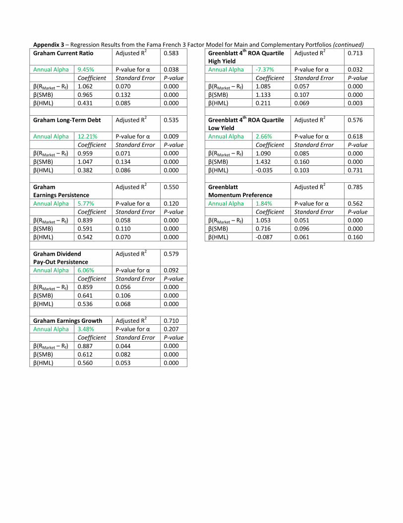
Appendix 3 – Regression Results from the Fama French 3 Factor Model for Main and Complementary Portfolios (continued)

Graham Current Ratio Adjusted R2 0.583 Greenblatt 4th ROA Quartile High Yield

Adjusted R2 0.713

Annual Alpha 9.45% P-value for α 0.038 Annual Alpha -7.37% P-value for α 0.032

Coefficient Standard Error P-value Coefficient Standard Error P-value

β(RMarket – Rf) 1.062 0.070 0.000 β(RMarket – Rf) 1.085 0.057 0.000

β(SMB) 0.965 0.132 0.000 β(SMB) 1.133 0.107 0.000

β(HML) 0.431 0.085 0.000 β(HML) 0.211 0.069 0.003

Graham Long-Term Debt Adjusted R2 0.535 Greenblatt 4th ROA Quartile Low Yield

Adjusted R2 0.576

Annual Alpha 12.21% P-value for α 0.009 Annual Alpha 2.66% P-value for α 0.618

Coefficient Standard Error P-value Coefficient Standard Error P-value

β(RMarket – Rf) 0.959 0.071 0.000 β(RMarket – Rf) 1.090 0.085 0.000

β(SMB) 1.047 0.134 0.000 β(SMB) 1.432 0.160 0.000

β(HML) 0.382 0.086 0.000 β(HML) -0.035 0.103 0.731

Graham Earnings Persistence

Adjusted R2 0.550 Greenblatt Momentum Preference

Adjusted R2 0.785

Annual Alpha 5.77% P-value for α 0.120 Annual Alpha 1.84% P-value for α 0.562

Coefficient Standard Error P-value Coefficient Standard Error P-value

β(RMarket – Rf) 0.839 0.058 0.000 β(RMarket – Rf) 1.053 0.051 0.000

β(SMB) 0.591 0.110 0.000 β(SMB) 0.716 0.096 0.000

β(HML) 0.542 0.070 0.000 β(HML) -0.087 0.061 0.160

Graham Dividend Pay-Out Persistence

Adjusted R2 0.579

Annual Alpha 6.06% P-value for α 0.092

Coefficient Standard Error P-value

β(RMarket – Rf) 0.859 0.056 0.000

β(SMB) 0.641 0.106 0.000

β(HML) 0.536 0.068 0.000

Graham Earnings Growth Adjusted R2 0.710

Annual Alpha 3.48% P-value for α 0.207

Coefficient Standard Error P-value

β(RMarket – Rf) 0.887 0.044 0.000

β(SMB) 0.612 0.082 0.000

β(HML) 0.560 0.053 0.000