Forecasting Excess Returns in the Housing Market with Local Cap

Rates

Stéphane Gregoir & Tristan-Pierre Maury∗

INSEE EDHEC Business School

Preliminary version

October 27, 2014

Abstract

We investigate the predictive power of rent-to-price ratios in an excess housing return equation. Relying on two

large geo-coded databases related on the one hand to rents and on the other hand to selling prices in the Paris

area from 1996 to 2007, we compile rent-to-prices ratios and price growth rates with individual modelings and

localized imputation methods. Different sources of risk (price, rent or vacancy risk) are taken into account. We

break down the contributions of this rent-to-price measurement on futures excess returns into different geographical

scale contributions: from broad scale (city level) to small scale one (the land register unit level corresponding to

a few building blocks). Comparing the forecasting power of rent-to-prices ratio at various spatial scales seems

relevant when working on housing markets composed of illiquid assets with a large idiosyncratic component, but

is not usually done by lack of data. The spatially-disaggregated forecasting equations are estimated with standard

techniques for different forecast horizons (3 and 6 years). The time dimension of the sample being short, we analyse

the impact of the small-sample bias on our estimates. We exhibit that rent-to-price ratios account for a substantial

part of the forecasting error at medium term horizon, the largest share of it being captured by the smallest scale

measure.∗Corresponding Author: EDHEC Business School, Paris Campus, 18 rue du Quatre Septembre, 75002, Paris, FRANCE. Tel: (+33)

(0)153327646. Fax : (+33) (0)153327631. email: tristan.maury@edhec.edu

1

A Introduction

Following a large literature in finance (see among others Fama and French, 1988), returns predictability in real estate

has been intensively studied. The predictive power of various factors (construction costs, per capita income, variables

related to demography, etc.) when forecasting real estate prices or returns has been assessed at several horizons and

spatial scales. The role of the cap rate (i.e. the rent-to-price ratio or rental return) has been singled out due to

the significant contribution generally evidenced for its stock market counterpart, the dividend-price ratio (Campbell

and Shiller (2001)). Its predictive power has been evaluated mainly using metropolitan or city-level datasets with

contrasted conclusions depending on the chosen metropolitan areas, spatial scale or asset type (housing, offi ce, retail,

etc.). Plazzi, Torous and Valkanov (2010) illustrate that cap rates performances vary greatly with the metropolitan

area (hereafter MA) under study. However, real estate prices and rents largely vary at the infra-metropolitan level

due to the existence of local markets (local housing stock characteristics, local amenities) so that trends for the whole

metropolitan may not reflect local market rigidities at smaller scales (city-level, building block level, etc.) that have

a direct impact on real estate price and rent dynamics. This neglected infra-MA heterogeneity may bias estimates

because of a spatial aggregation bias, see Smith (2004). We here evaluate the predictability of local housing returns

using properly measured cap rates at different spatial scales (from building block level to city level) as predictors. Our

localized cap rate measures are indeed an average of individual rent-to-price ratios different from the average rent to

average price ratio usually computed in the literature, measure subject to statistical bias affecting the quality and

interpretation of the estimates in this kind of regressions.

When adopting an asset price perspective, the price of a real estate asset should equal the present value of

its future expected rents. This implies that the dynamics in real estate prices mainly reflects variations in future

expected rents or in future discount rates that vary across local markets depending on land availability, existing and

planned amenities, etc. Recently, Campbell, Davis, Gallin and Martin (2009) proposed a variance decomposition of

the rent-price ratio for 23 U.S. MAs housing markets. The rent-price ratio is split into the expected rents growth

component and the expected real interest rates and housing premia components (these last two terms are part of the

total expected return). They found significant time-variability of these components (as well as a significant correlation

between these terms) which explain a substantial part of the cap rate heterogeneity.

This evidence of a large amount of heterogeneity in cap rates is in line with financial market observations that

led to question the predictive power of dividend yields to forecast stock returns. A large literature in finance has been

devoted to these problems1 . The corresponding real estate literature is much smaller partly due to a lack of individual

1See for example Fama and French, 1988, or Cochrane, 2008, for papers concluding to a significant returns predictability or Campbell

2

observations which implies the use of proxies that can affect the quality of empirical results. Mankiw and Weil (1989)

or Case and Shiller (1990), working at different (large scale) levels, fail in detecting a significant relationship between

rent-price ratios and subsequent changes in prices or excess returns. Meese and Wallace (1994) used time-series data

on housing prices, rents and the user cost of capital for two Northern California counties (Alameda and San Francisco)

and validate the housing present value model in the long run with data running from 1970 to 1988. Capozza and

Seguin (1996) studied expectations of capital gains in the U.S. housing market. Using census data disaggregated by

metropolitan areas, they show that cross-sectional cap rates have significant power in predicting 10 years capital gains.

Clark (1995) using a methodology close to Capozza and Seguin (1996) and decennial census-tract level data from 1950

to 1980 finds a significant and negative relation between rent-price ratios and next 10 years’rent growth rates. In a

VECM framework controlling for the role of direct user costs, Gallin (2008) provides evidence of a significant long-run

relationship between prices and rents for whole-US housing quarterly data from 1970 to 2005. Finally, in line with

the present value model, current cap rates appear to be significantly linked negatively to future changes in rents and

positively to future changes in prices.

Recently, Plazzi, Torous and Valkanov (2010) extended the previous studies to apartments and retail, industrial

and offi ce properties. They adopt a long horizon approach (similar to Gallin, 2008) and investigate whether the cap

rate reflect fluctuations in expected returns and/or in rent growth rates, building on a version of Campbell and Shiller

(1988)’dynamic Gordon growth model. According to this model, high cap rates should reflect either higher future

discount rates or lower expected rent growth rates. Using prices and cap rates for each property type on a quarterly

basis from 1994 to 2003 for 53 U.S. metropolitan areas in a GMM framework, they estimate long-run predictive

equations at different forecast horizons (1, 4, 8 and 12 quarters) controlling for inter-MA heterogeneity with various

local demographic or economic factors. They provide evidence that higher cap rates predict higher future returns for

the various types of real estate, offi ce properties excepted. Their results also seem to confirm previous findings in the

case of stocks (Fama and French, 1988): the predictive power of cap rates (or dividend yields) is stronger for long

forecast horizons.

The most recent contributions to the literature of predictability in real estate find a significant power of cap

rates for predicting returns. But, in most cases no individual estimation of rents is provided: some of the above

papers use individual price data, but MA (or national) average for rents. These studies (except Clark, 1995) then

evaluate the predictive power of cap rates at the MA level. However, we may reasonably expect that a large part

of the information conveyed by cap rates is relevant at an infra-MA or infra-city level: due to the possibly high

and Shiller, 2001, who did not find any significant forecasting power of the dividend-price ratio.

3

heterogeneity in the housing stock characteristics within a MA and its persistence, a large variability in buyers and

sellers’socio-demographic profiles may exist, thereby conducting to heterogeneity in expectations and then in local

cap rates. Differently said, there may be more difference between the expected average discount rates (or risk premia)

in a wealthy and low-income areas of a MA than between the wealthiest areas of two distinct MAs. Moreover, most of

the real estate market actors collect information at a local level to base their decisions. Small-scale gaps in cap rates

may then reflect diffi culty in getting reliable informations (available data are noisy and involve lenghty and costly

compiling processes) on future trends in rent (expected payoffs for a new owner) or in prices.

We give here a first micro-level account of the predictive power of cap rates on excess returns in checking if the

relationship between current cap rates and future returns is valid at the local level, i.e. the convenient scale of market

functioning and information availability, and in assessing its magnitude. A possible aggregation bias resulting from

the use of ratio of aggregate indexes as proxy for cap rates has to be studied. We empirically illustrate that this bias is

not constant and part of the dynamics in cap rates may result from it. At last, we can add that none of the preceding

contributions take the vacancy risk into account. Such measures are only available for commercial real estate (see

NCREIF or IPD indexes for example) and use appraisal-based data instead of transaction-based data. Consequently,

these measures suffer from numerous well established shortcomings: oversmoothing (the true amount of volatility is

underestimated) and lagging (time lag in detecting turning points), see Geltner (1997) for a comprehensive study on

the limitations of these appraisal based measures.

Using two very large French databases, we produce a local measure of cap rates, capital appreciations, total

returns and associated risks over the last housing boom that affected the French real estate market. We use the admin-

istrative registration by notaries of all the housing transactions between 1996 and 2007 (about 1, 000, 000 transactions)

in inner Paris and a panel of about 27, 000 rented flats or houses surveyed on a yearly basis in the same area. On

the one hand, we estimate local hedonic price equations with the first database. It is combined with a repeat-sale

type approach for a subset of about 7% of the sample in order to assess the average individual time correlation of the

unexplained part of the hedonic equations. On the other hand, we estimate hedonic rent equations as well as occupa-

tion/vacancy spell equations with the second data base. These models allow us to impute local rent and occupation

periods and measure real estate returns (cap rates and price growth rates). We provide estimates of local means of

housing returns on Paris and its first suburbs for the 1996—2004 period.

We then estimate spatially-disaggregated forecasting equations with standard techniques for different forecast

horizons (3 and 6 years). The time dimension of the sample being short, we analyze the impact of the small-sample

bias on our estimates. Moreover, we break down the contributions of this rent-to-price measurement on futures excess

4

returns into different geographical scale contributions: from broad scale one (arrondissement or precinct for example)

to smaller scale one (the land register unit level corresponding to a few building blocks). Our results suggest that cap

rates may serve as a leading indicator of future excess returns in line with Plazzi, Torous and Valkanov (2010). They

account for a substantial part of the forecasting error at medium term horizon, the largest share of it been captured by

the more local measure. Most of the local future trends is conveyed by local —instead of global —current indicators.

This paper is organized as follows. Section 2 presents the rental market and our databases. Section 3 exposes

models for rents and prices, as well as cap rates and capital price increases construction method. Section 4 presents

the forecasting equations. Section 5 analyses the dynamic relationship between cap rates and capital appreciations

(or excess returns) at different spatial scales. Section 6 concludes.

B Rental Market and Data Presentation

B.1 The rental market

The size of the rental housing stock, excluding the public sector, was almost one million dwellings2 in Paris Region on

January 1st , 2008 according to OLAP (Observatoire des Loyers de l’Agglomération Parisienne —French observatory

of rents for Paris Region) with 400, 000 dwellings in Paris itself, 380, 000 dwellings in the inner suburbs3 and 210, 000

dwellings for Paris’s outer suburbs4 . Hence, the rental estate is highly concentrated in the centre of the Paris region.

During the last ten years, the size of the rental stock has decreased in Paris and increased in the suburbs due to

growing urbanization, housing tax cuts, and subsidies for investors. For example, in the outer suburbs, almost half of

the rental housing stock was built after 1975. Such recent buildings only account for 15% of the rental housing stock

in Paris and 32% in the inner suburbs. In Paris, 66% of the dwellings were built before 1949 (especially during the

second half of the 19th century, the Haussmann period) against 17% in Paris’s outer suburbs.

2This estimation is based on INSEE (French National Statistical Institute) census data3The inner suburbs consist of three départements (administrative units): the Hauts-de-Seine, the Seine-Saint-Denis and the Val-de-

Marne.4The outer suburbs consist of four départements : the Seine-et-Marne, the Yvelines, the Essonne, and the Val d’Oise. We only consider

that part of the outer suburbs contained within Paris’s metropolitan area.

5

Table 1: Rental Housing Stock by Construction Period

Construction Period Paris Inner Suburbs Outer Suburbs

< 1949 67.3% 34.8% 17.1%

1949− 1974 18.0% 33.4% 37.9%

1975− 1989 9.0% 13.4% 19.0%

> 1989 5.7% 18.4% 26.0%

The floor area of housing is correlated to the building construction period (for example, many Haussmann

period buildings in Paris are quite small). Table 2 shows that the main part, 66.8%, of the housing stock in inner

Paris is ‘studio’or ‘one bedroom’. This part is lower in the inner suburbs (56.6%) and the outer suburbs (45.8%).

The distribution of the rental housing stock according to the dwelling floor area is quite different from the distribution

of the total housing stock: in 2006, the share of studios apartments in the total housing stock in inner Paris was

22.6% (30.8% for the rental housing stock) and the share of ‘more than 2 bedrooms’dwellings was 24.1% (14% for

the rental stock). Similarly, in Paris’s close periphery, the share of studio apartments in the total housing stock was

10.8% (22.4% for the rental sector) and the share of ‘more than 2 bedrooms’dwellings was 36.9% (16.8% for the rental

stock). Hence, small dwellings are more frequently on the rental market. This relative scarcity of large dwellings in

the private rental housing sector might be responsible for their low vacancy rate (which will be evidenced below).

Table 2: Rental Housing Stock by Number of Rooms

Bedrooms number Paris Inner Suburbs Outer Suburbs

0 (studio) 30.8% 22.4% 19.0%

1 bedroom 36.0% 34.2% 26.8%

2 bedrooms 19.2% 26.6% 27.0%

> 2 bedrooms 14.0% 16.8% 27.2%

Consequently, we choose to focus our analysis on Paris itself due to the relatively small size of the rental sector in

Paris’s suburbs (especially the outer suburbs). Moreover, since the outer suburban area is very large, the rental estate

is irregularly spatially distributed which might lead to poor hedonic estimations. We also only consider second-hand

apartments: new dwellings and houses only represent a small share of the total transactions for the Paris Region, and

their price/rents and structural attributes differ greatly from those of second-hand apartments.

In the rental market, the rent of vacant housing is the result of a free bargaining between the owner and the

tenant. However the evolution of the rent paid by the sitting tenant follows that of the national reference index

(IRL– Indice de Référence des Loyers) based on the inflation rate and the growth of construction costs. The very

6

large majority of lease contracts has a three-year duration (other types of contracts are excluded from our analysis).

Contracts are renewable and rents are revised on an annual basis (according to the one-year growth rate of the IRL).

B.2 Dataset for the rental market

Our dataset for the private rental sector in Paris Region comes from a survey carried out by OLAP of approximately

25, 000 housing units over a representative sample of the rental market in inner Paris. Each year, more than 7, 000

housing units in Paris are surveyed (the sampling rate is 1/80). This is a panel survey, each dwelling being regularly

surveyed (every two or three years on average). Information is mainly gathered from the property manager (more than

80% of the whole dataset), rather than from the tenant or owner of the dwelling. This enables precise estimates of

occupation or vacancy duration and rent evolution for each asset. The survey data includes information concerning

the following: the current occupancy status of the housing unit (vacant/occupied), the current rent when the housing

unit is occupied, the duration of residence of the current tenant (when occupied) as well as the date of the last rent

revision, the duration of vacancy (when vacant) and the duration of residence (and rent evolution) of the preceding

tenant.

Our empirical analysis is then based on a housing unit event-history sample. The frequency of the survey

enables an almost complete (for more than 96% of the sample) reconstitution of the occupancy status and rent history

for each housing units in the sample. Even if there has been more than one tenant change between the two survey’s

dates, the missing information can generally be collected from the property manager.

The panel is regularly renewed, since some units may exit the survey (either because the surveyor did not find

any respondent or because the unit is now occupied by the owner). The dataset also includes precise information on

the unit structure type (floor area, floor level, construction period, number of rooms, elevator, number of bathrooms,

number of garages, etc.). The attributes included in the duration and hedonic model final specifications will be further

set out. Many other housing attributes regarding the comfort of the unit have been discarded because no corresponding

item was available in the dataset on transaction prices. Moreover, detailed information regarding the location of the

unit is available (here ranked from the larger to the finest geographic scale):

• The postal code. It gives the district (arrondissement) where the asset is located. Fig. 1 provides a map of Paris

by district. The 9th district where some geographical refinements will be provided (Figs. 2 and 3) is in red.

• The administrative precinct (quartier). Each Parisian district is divided into four precincts (the smallest admin-

istrative units for Paris). Fig. 2 provides a map of the four precincts of the 9th district of Paris.

7

• The land register unit (section cadastrale) for each Parisian precinct. It is the lowest geographic scale available

in the survey. Each land register unit is delimited by major streets and comprises approximately ten building

blocks. Fig. 3 provides a map of the units of the 9th district of Paris. There are approximately 1388 land register

units in inner Paris.

B.3 Dataset for sales

The dataset on housing unit sales comes from the Paris Region Chamber of Notaries (CINP– Chambre Interdéparte-

mentale des Notaires de Paris). In France, all property sales have to be registered by a notary, who collects the realty

transfer fee to be paid to the Inland Revenue. The database includes information on the transaction price, along with

detailed characteristics– the main variables are: floor area, floor level (for apartments, date of construction, number

of garages, number of bathrooms, elevator/no elevator– precise location (postal code, precinct, land register unit) and

transaction date (month) for each dwelling.

The global dataset consists of exactly 1,064,528 housing unit transactions for inner Paris. The coverage rate

is approximately 90%. We restrict our sample to second-hand flat transactions. New flats and houses only represent

a very small share of the total sales in Paris, and their price and structural attributes differ greatly from those of

second-hand apartments. Moreover, transfer fees are not the same for new and second-hand properties.

C Returns construction methodology

The presentation of our model is divided into two parts: (1) the joint estimation of a model for rent and duration

of occupancy and vacancy for the rental market, (2) the estimation of a model for transaction prices for the housing

sales market. Notice that a complete model presentation is made in Gregoir et al. (2012).

C.1 Model for the rental market

The panel structure of our sample allows us to identify a set of specific effects: (i) We follow individual units for a long

period and many have multiple spells which permits identification of an unobserved heterogeneity term (see Honoré,

1993, or Abbring and Van den Berg, 2001), (ii) we are also able to estimate the impact of the previous vacancy

duration of a unit on the initial rent for the new tenant, (iii) the link between the current rent of an occupied unit

and the probability of a transition to the vacant state is also estimated.

8

We simultaneously estimate two distinct discrete-time duration models for units in the vacant state (eiτ = 0)

or in the occupied state (eiτ = 1) with i = 1, ..., N indexing the housing unit and τ the calendar date. N is the total

number of assets in the dataset.

C.1.1 Transition from vacant state

Let hvj(i),τ (.) be the exit rate from the vacant to the occupied state for unit i at the calendar date τ . t is the duration

spell (in the vacant state). The exit rate is defined as follows:

hvτ (t | xiτ , ωvi ) = Pr (T viτ = t | T viτ > t− 1, xiτ , ωvi ) (C.1)

where xiτ (including an intercept term) is a vector of physical, local and time attributes for asset i at date τ . Notice

that xiτ also includes spatial dummies q (i) (i.e., precincts). ωvi is a fixed unobserved factor. T viτ is the vacancy

duration for unit i at date τ . Let us consider a model for capturing both duration dependence and business cycle

effects:

hvτ (t | xiτ , ωvi ) = G (x′iτα+ γvτ (t) + ωvi ) (C.2)

where G (.) is the cumulative logistic distribution function. γv (t) is a term capturing duration dependence. The vector

of parameters α evaluates the impact of the components of vector xiτ on the exit rate. In vacancy equation (C.2),

the final specification for xiτ will include the following variables: construction period, number of rooms, geographic

and year dummies. Other variables (floor area, number of bathrooms, floor level, elevator) have been excluded with

preliminary tests (see Gregoir et al., 2012 for a full presentation of covariates selection procedure). The business cycle

effect is introduced via calendar dummies included in x. Some housing units can differ in non observed attributes

(i.e., not included in x). This could be responsible for spurious duration dependence effects in the model estimation.

For example, dwellings in bad repair will stay vacant for longer periods than others, which can induce a negative

duration dependence effect, i.e., γv (t) decreases as t grows. Exit rate functions are then estimated conditionally on

an unobserved factor ωvi . The distribution of ωvi is supposed to be independent of x, but potentially linked to other

heterogeneity terms (see below).

C.1.2 Transition from occupied state

Let hoτ (t) be the exit rate from the occupied to the vacant state for unit i at calendar date τ . The interpretation

of this function is similar to that of the transition rate from the vacant state and we keep the same functional form,

9

except for the introduction of a current rent term:

hoτ (t | xiτ , ωoi ) = G (x′iτβ + γoτ (t) +Riτθ + ωoi ) (C.3)

The interpretation of βj(i), γoτ (t) and ωoi is similar to that of αj(i), γ

vτ (t) and ωvi in (C.2). The impact of the current

rent (at calendar date τ) Riτ for unit i on the transition probability is measured by θ. Ceteris paribus (x is similar

to the vacancy equation and then include spatial and temporal dummies), the higher the current rent, the higher is

the vacancy risk. The probability a tenant may leave their current dwelling increases when the rent is higher than

those of neighboring flats with similar attributes (depending on local supply). We hence expect positive values for the

estimators of θ.

C.1.3 Rent determination

For the estimation of the initial rent level, we rely on a usual hedonic model– i.e., including housing attributes as

explanatory variables– and we add the past duration of vacancy. Let Riτ be the initial rent (i.e., for a new lease with

a new tenant) of unit i at date τ . This rent depends on observable physical attributes, the location of the dwelling,

the date the lease was signed (included in x), the prior vacancy duration diτ , and unobserved heterogeneity factors.

We choose a logarithmic specification:

log(Riτ)

= x′iτφ+ ηdiτ + ωri + εiτ (C.4)

φ are the usual hedonic parameters. η gives the contribution of the vacancy duration. This parameter captures two

(opposite) effects. On the one hand, the longer a dwelling has been vacant, the lower the new rent to reduce non

productive capital costs. On the other hand, if the dwelling was renovated during the vacancy period, the requested

rent will be higher. ωri is an unobserved heterogeneity term with specification similar to ωvi and ω

oi . εiτ is a potentially

heteroskedastic Gaussian error term, εiτ ∼ N(0 , σ2ε,i,τ (xi)

). The specification of the variance-covariance matrix of

innovations is detailed in Gregoir et al. (2012). Let g(Riτ | xiτ , diτ , ωri

)be the density of the initial rent conditional

on observed and non observed factors. Notice that the value of the current rent Riτ+k at calendar date (τ + k) of

a housing unit occupied for k periods is easily deduced from the value of the new rent Riτ . The ratio of these two

rents is given by the cumulative growth rate πτ,τ+k of the IRL (Indice de Référence des Loyers) between τ and τ + k,

Rijτ+k = πτ,τ+kRijτ .

10

C.1.4 Estimation

Let Li (ωvi , ωoi , ω

ri ) be the likelihood for asset i conditional on x (omitted from the argument of the function to keep

notations simple) and on unobserved factors ωi. The joint distribution of the three heterogeneity terms of vector

ωi = (ωvi , ωoi , ω

ri )′ (corresponding, respectively, to the duration model from the vacant state, from the occupied state,

and to the hedonic rent model) is assumed to be normal ωi ∼ N (0,Ω). Ω is supposed to be time homogenous. We

have to estimate the three variance terms σ2ξ (ξ = v, o and r) and three linear correlation terms ρov, ρor and ρrv. The

time period of our monthly sample is [1996(1) ; 2007(12)]. Let ni be the total number of transitions (from vacancy

to occupancy and conversely) of dwelling i during that period. ςi = τ i,1, ..., τ i,ni is the set of calendar dates of

transitions. τ i,0 is the date of the entry of dwelling i in the database (τ i,0 ≥ 1996(1)) and τ i,ni+1 is the date of exit

(τ i,ni+1 ≤ 2007(12)). We finally get the following formulation of the joint conditional likelihood Li (ωvi , ωoi , ω

ri ):

ni+1∏k=1

τ i,k−1∏

l=τ i,k−1+1

[1− hvil (l − τ i,k−1, ωvi )]hv

iτ i,k(τ i,k − τ i,k−1, ωvi ) g

(Riτ i,k | xiτ i,k , τ i,k − τ i,k−1, ωri

)1−eiτi,k−1

×

τ i,k−1∏

l=τ i,k−1+1

[1− hoil (l − τ i,k−1, ωoi )]ho

iτ i,k(τ i,k − τ i,k−1, ωoi )

eiτi,k−1

with hf

iτ (t, ω) = hfiτ (t, ω)1−ci

[1− hfiτ (t, ω)

]cif = v, o where ci is a variable indicating whether the observation is

right-censored (ci = 1) or not (ci = 0). We deduce the contribution of housing unit i to the joint non conditional

likelihood:

Li =

∫Li (ωvi , ω

oi , ω

ri ) dF (ωi)

where F (.) is the cumulative normal distribution function with variance-covariance matrix Ω. The joint likelihood for

the whole sample is L =

n∏i=1

Li. The complete model of durations (occupation and vacancy) and rents is estimated

with maximum likelihood techniques. The duration models are estimated using the occupational status history from

January 1996 to December 2007 of 26, 957 housing units located in Paris.

C.2 Sale price model

For the determination of transaction prices, we use a standard hedonic model. Let Piτ be the (potentially theoretical)

price of a housing unit i at date τ . Let xiτ be the vector of physical attributes of dwelling i. Note that this vector is

not exactly similar to the one employed in the rental model xiτ (C.4): some of these characteristics available in the

OLAP dataset are not available (or differently recorded) in the notarial dataset. The price hedonic equation is

log (Piτ ) = ψk(i,τ)xiτ + υiτ (C.5)

11

ψk(i,τ) is the vector of hedonic parameters and k (i, τ) is the spatial and temporal estimation area for the price model.

Notice that the price estimation area differs from the one employed for the rent model, j (i). Indeed, the number of

sale transactions in the Paris region is much higher than the number of new leases which enables geographical and

temporal refinements. A separate model will then be estimated for each year τ and each administrative district. υiτ

is the zero mean error term. Its variance σ2υ,i,τ depends on certain structural attributes (i.e. the number of rooms)

and on the spatial and temporal estimation area of unit i.

We choose a log-log specification (the floor area is the sole continuous explanatory variable and is specified in

logarithm ; other dummy variables are the number of rooms, the construction period, floor level, elevator, number of

bathrooms, garage, time and location dummy variables and seasonality effects). Eq. (C.5) is estimated with two-stage

least squares to control for heteroskedasticity.

C.3 Cap rates and capital appreciation

For each apartment i = 1, ...., N , with a land register unit localization and for each year of transaction since 1996, we

calculate the housing returns (cap rates and capital appreciation are separately evaluated). Our measure of housing

return is associated to the following strategy: a real estate investor buys a housing unit i at the beginning of the year

corresponding to τa (January, 1st exactly). The transaction price is Piτa . The investor puts the dwelling on the rental

market. We consider only three-year leases (the most frequent on the French market). The ratio of received rent flows

Riτ for τa ≤ τ ≤ τa + 36 (taking vacancy risk into account) over the initial price Piτa is the cap rate of the asset.

Three years later in (τa + 36), i.e., the soonest point at which the lease could end or be renewed, the lessor wants to

put the asset up for sale. The capital appreciation will be the ratio between the sale price Piτa and the purchase price

Piτa+36. However, such a sale is only possible at lease maturity. If at least one tenant’s change happened over the

[τa, τa + 36] period or if the owner did not find a tenant immediately (at date τa), the apartment will not be available

for sale on January 1st of the year corresponding to (τa + 36). In such a case, the owner has two possibilities: (i) sell

the occupied asset and transmit the lease, (ii) wait for the lease term or for an early departure of the current tenant

and then put the (free) asset up for sale. In the first case, the rebate we observe for such sales in the database is on

average large (approximately 20% cheaper) and with a large variance. The notaries dataset does not permit a detailed

evaluation of the impact of each housing attribute on this price gap. Consequently, we adopt strategy (ii) and suppose

that the owner puts the asset for sale from the moment it becomes vacant.

We now present the methods for the evaluation of individual and localized cap rates and price gains (the full

computational details are provided in Gregoir et al., 2012). For the calculation of cap rates, we propose the following

12

imputation technique: for each purchase date τa and each housing unit attribute xia , let s (i) denote the land register

unit where dwelling i is located. We use the estimated hedonic price equation and simulate 10 purchasing prices Piτa

by bootstrapping among residuals located in s (i). We then simulate 10 rental paths for housing unit i from purchase

date τa until the random selling date τv. For each path, we obtain occupation and vacancy periods with (C.2) and

(C.3) and bootstrap newly bargained rents with (C.4) for each transition form vacancy to occupation. Notice that due

to the reduced number of rent observations per land register unit, we cannot perform all drawings for unit i within the

same register unit s (i).We enlarge the imputation area with a standard Spatial AutoRegressive SAR model estimated

for each precinct q (i). With ten simulated rent paths and ten purchasing prices, we obtain 100 combinations for

the cap rate capi,τa of specific unit i. The yields are then annualized. These returns are individual (same physical

attributes for the simulated rent paths and purchasing price) and localized at the land register unit level.

For the capital appreciations of housing unit i and purchase date τa, we keep the 10 previously simulated

purchasing prices Piτa and now simulate resale prices Piτv at random selling date τv. Notice that drawings of

purchasing and resale prices should not be done independently, since they concern the same unit i: the weak explanatory

power of the hedonic price model implies that a remaining volatility could impact our measure of average returns. We

then use an imputation technique in the spirit of the repeat-sales approach. We finally obtain individual and localized

simulation of capital appreciation 4Pi,τa of specific unit i at purchase date τa. The total return Ri,τa is simply the

sum of capi,τa and 4Pi,τa .

C.4 Descriptive results

Over the considered period [1996-2007] and area (inner Paris), we show the existence of temporal and geographic

disparities in cap rates and total returns. Thus, since 1996, we see a continued decline in cap rates on all Paris

districts. For example, the average rental yield (in real terms and annualized) in Paris decreased from 5.14% in 1997

to 2.49% in 2004 (see Table 3). This is due to the sharp rise in transaction prices on the whole [1996− 2007] period:

more than 164% increase for second-hand apartments in Paris against only 40% for rents. The strong regulatory

constraints on the evolution of private leases likely contributed to limit their growth, which may explain such a

discrepancy with the trends in prices.

Meanwhile, total returns also experienced very marked movements over the period considered. In the mid-1990s,

when prices rose only very slightly or stagnated in some districts, the total returns were relatively small, close to 10%

in 1997. Following the sharp general rise in prices in the mid-2000s, capital yields rose sharply to reach levels close to

14% in 2002.

13

Table 3: Average cap rates and total returns in Paris per year (real, annualized)

1997 1998 1999 2000 2001 2002 2003 2004

capi,τ 5.14% 5.03% 4.23% 3.67% 3.22% 3.43% 2.70% 2.49%

Ri,τ 10.40% 12.14% 13.87% 12.21% 13.02% 13.83% 11.82% 9.08%

The cap rates capi,τ and total returns Ri,τ are also geographically very heterogeneous and these spatial dispar-

ities are quite persistent. Indeed, we observe significant differences between cap rates in the North East (see Figures

4a and 4c below for an example) in Paris (about 6% between 1997 and 2000) and those from central Paris (steadily

below 5% over the same period for the first seven districts). In the late 2000s, these differences in local cap rates are

still present and have not been dampened by the sharp rise in values: about 3% in the North East against only 2% in

the center of Paris. Historically, the cheapest precinct/register units of Paris are also those where the rent-prices are

higher, which stems from a great range of dispersion of transaction prices compared to rents.

[ Insert Figures 4a,4b,4c,4d ]

The spatial heterogeneity of Ri,τ is equally marked (see Figures 4b and 4d for capital gains, recall that Ri,τ is

the sum of the cap rates, capi,τ , and capital gains) : between 1997 and 2000, capital gains were high in the fourth,

sixth and seventh districts, where the recovery of real estate values had already begun, while those gains were smaller

(sometimes close to zero) in some districts of North East of the capital. Instead, over the period [2004-2007], our returns

measures showed a reversal of this trend: the highest increases in selling prices have been observed in the North East

of Paris, which resulted in capital gains well above those of the first seven districts. Inter-district differences in capital

gains increased over time.

However, it appears that a simple comparison of yields by district in Paris is not enough. The spatial het-

erogeneity of returns to Paris is much thinner: working with averages of yields by district can lead to losing a lot

of information on differences across precinct or small neighborhoods. Accordingly, we propose measures of cap rates

and total returns for three different geographic levels: (a) by district, (b) by precinct (each district comprises four

administrative precincts, (c) by land register unit (each district comprises between 25 and 150 land register units,

each involving about ten/fifteen buildings). Table 4 below provides with the average standard deviations of returns

(cap rates and total returns) across Parisian districts, then across precincts of the same district, and finally across all

land register units of the same precinct. We present these results from 1996 to 2004.

14

Table 4: Standard deviation of cap rates and total returns per year and per geographic level

1996 1997 1998 1999 2000 2001 2002 2003 2004

capi,τ - district 0.6504 0.6681 0.7833 0.7739 0.7451 0.7553 0.6948 0.5513 0.4457

capi,τ - precinct (same district) 0.3749 0.4088 0.4828 0.4810 0.4629 0.4553 0.4422 0.3419 0.2711

capi,τ - land unit (same precinct) 1.0434 1.1186 1.1508 1.1783 1.1269 1.0608 1.0154 0.8289 0.7019

Ri,τ - district 2.5432 2.8556 2.7890 2.0984 1.8899 2.5641 3.2919 3.7751 2.8193

Ri,τ - precinct (same district) 1.1574 1.2507 0.9801 0.9909 0.9654 1.0660 1.7121 1.2994 0.9080

Ri,τ - land unit (same precinct) 4.5416 4.6930 4.5102 4.0251 4.3631 4.3323 4.4712 3.9335 3.5528

These results show that much of the variability of returns is at a sub-district and even sub-precinct level. In

particular, in 2004, a large share of the total geographical variability of cap rates is due to differences across land

register units of the same administrative precinct (a somewhat smaller fraction is due to differences between the four

precincts in the same district). This variability at the land unit is even greater for total returns. These measures show

how unobserved local factors (such as the presence of utilities, retails, etc.) can influence rental values and transactions

prices and then potentially yields. Using a simple aggregate measure can lead (in addition to statistical bias that will

be shown later) to smooth out these differences and thus lose some of the critical information needed to measure and

predict changes in yields. We now turn to the illustration of the predictive power of this additional information (yields

measured at the land register unit level) on future trends in excess returns.

D Forecasting equations

D.1 Framework

In line with the literature, we consider the following endogenous variable y: the excess housing return (see Case and

Shiller, 1990, or Plazzi, Torous, Valkanov 2010). We set yl,t = log (Rl,t)− log (rt) where l stands for the land register

unit and t = 2002, ..., 2007 for calendar year of resale. Rl,t is the total housing return. rt is the real 10 years French

treasury bond rate. Let Yt = y1,t, ..., yn,t be the vector of all excess returns at date t. n is the size of the total set

of land register units. In the rest of the paper for sake of notational simplicity, we assume that the panel structure is

homogenous. There are L land register units per precinct, P precincts per district and D districts. In practice, if P

is fixed, L varies with the precinct.

The usual framework in finance to analyze the predictive power of a univariate variable xt to forecast a univariate

15

variable yt corresponds to the following set of equations

yt = α+ βxt−1 + ut

xt = γ + δxt−1 + vt

with various distributional or probabilistic assumptions on (ut, vt) but in particular the existence of a non-zero con-

temporaneous correlation between the two error terms. This correlation generates a finite-sample bias problem for the

estimation of β that has been discussed in detail in particular when (xt)t is near integrated (Nelson and Kim (1993),

Stambaugh (1999), Amihud and Hurvich (2004), Lewellen (2004), Campbell and Yogo (2006) inter alios). We want

to modify this framework to capture the influence of the different geographical scales. We thus have to complement

a predictive regression with a set of equations stating the dynamics of the cap components associated to each scale.

A direct extension of the above set of equations is under the assumption that |δl| < 1, |δp| < 1 and |δd| < 1, for

t = 1, ..., T

yl,t = α+ βl [xl,t−1 − xp,t−1] + βp [xp,t−1 − xd,t−1] + βd [xd,t−1 − xw,t−1] (eq1)

+η1,l,t + ε1,p,t + ξ1,d,t

[xl,t − xp,t] = δl [xl,t−1 − xp,t−1] + η2,l,t (eq2)

[xp,t − xd,t] = δp [xp,t−1 − xd,t−1] + ε2,p,t (eq3)

[xd,t − xw,t] = δd [xd,t−1 − xw,t−1] + ξ2,d,t (eq4)

where xz,t = log (capz,t) is the average log of cap rates at the land register unit (z = l), precinct (z = p), district

(z = d) or whole inner Paris (z = w) level.[xl,t − xp(l),t

]is the deviation of log cap rates at the land register unit level

from its own precinct average (denoted p).[xp,t − xd(p),t

]and [xd,t − xw,t] may be interpreted in a similar manner.

yl,t is the annualized excess return between purchase date t − 3 and resale date t and xz,t−1 is the log of cap rates

derived from flows of rents between t − 4 and t − 1 with z = l, p, d or w.(η1,l,t, η2,l,t, ε1,p,t, ε2,p,t, ξ1,d,t, ξ2,d,t

)is

the six dimensional error term such that the three couples(η1,l,t, η2,l,t

),(ε′1,p,t, ε2,p,t′

)and

(ξ1,d,t′′ , ξ2,d,t′′

)are not

correlated for any couple of dates (t, t′) , (t, t′′) or (t′, t′′). The key identifying assumption is that there exists a non-zero

contemporaneous correlation between the components of(ηl,1,t, ηl,2,t

), (εp,1,t, εp,2,t) and

(ξd,1,t, ξd,2,t

), but not across

spatial scales. An important point is that yl,t (which incorporates the cap rates) and (xl,t−1, xp,t−1, xd,t−1, xw,t−1) are

overlapping on the [t− 3, t− 1] period. [xl,t−1 − xp,t−1], [xp,t−1 − xd,t−1] and [xd,t−1 − xw,t−1] are then endogenous

in equation (eq1). We model this endogeneity through the correlation of(ηl,1,t, ηl,2,t

), (εp,1,t, εp,2,t) and

(ξd,1,t, ξd,2,t

).

16

A slightly different framework would have been a similar specification for the equations of yt and xt as follows

yl,t = α+ βlxl,t−1 + βpxp,t−1 + βdxd,t−1 + η1,l,t + ε1,p,t + ξ1,d,t (D.7)

xl,t = γ + δlxl,t−1 + δpxp,t−1 + δdxd,t−1 + η2,l,t + ε2,p,t + ξ2,d,t (gen_cap)

We nevertheless choose to work on the set of equations (eq1,eq2,eq3,eq4) which corresponds to the set of within

equations derived from (D.7) (notice that implicitly the contemporaneous error terms at a given scale level have a

sum equal to zero, this has to be taken into account in the derivation of small sample bias).

This modelling allows us to break down the contributions of cap rates on future excess returns at different

geographical scales, the respective impact of the land register unit, precinct and district being measured by βl, βp and

βd. If these impacts are equal, the first equation reduces to a standard one

yl,t = α+ βl [xl,t−1 − xw,t−1] + η1,l,t + ε1,p,t + ξ1,d,t

In the specification of the log cap rate dynamic equation, there is no intercept because we work with the deviations

from the average of units of the same geographical sets. We are agnostic about the possible near-integratedness of

the different log cap components. The empirical analysis will allow us to consider this question. This set of equations

(eq1,eq2,eq3,eq4) does not correspond to a multivariate dynamic panel data model, each equation is related to a

different level of observation and the associated sample size varies accordingly. The two first equations are associated

to L × P × D × T observations, the third one to P × D × T observations and the last one to D × T observations.

The error terms are nevertheless correlated. We can deal separately with each equation in introducing in equation

(eq1) the contemporaneous values of(xl,t − xp,t xp,t − xd,t xd,t − xw,t

)′which corresponds to the triangular

representation of the three bivariate time series (Cholevsky factorization of each (2× 2) variance covariance matrix of(ηl,1,t, ηl,2,t

), (εp,1,t, εp,2,t) and

(ξd,1,t, ξd,2,t

)).

D.2 Small sample bias correction

We therefore work on the following triangular autoregressive model

yl,t = α+

1∑j=0

αj,l [xl,t−j − xp,t−j ] +

1∑k=0

αk,p [xp,t−k − xd,t−k] (D.8)

+

1∑i=0

αi,d [xd,t−i − xw,t−i] + η∗1,l,t + ε∗1,,t + ξ∗1,d,t

17

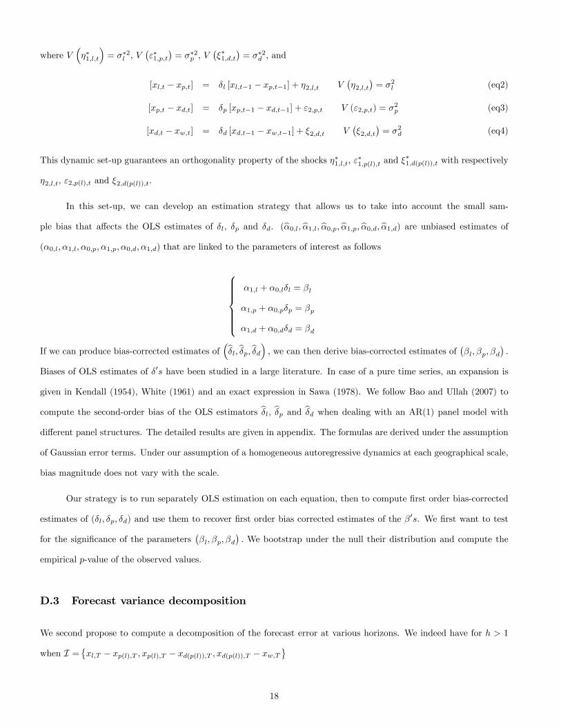
where V(η∗1,l,t

)= σ∗2l , V

(ε∗1,p,t

)= σ∗2p , V

(ξ∗1,d,t

)= σ∗2d , and

[xl,t − xp,t] = δl [xl,t−1 − xp,t−1] + η2,l,t V(η2,l,t

)= σ2l (eq2)

[xp,t − xd,t] = δp [xp,t−1 − xd,t−1] + ε2,p,t V (ε2,p,t) = σ2p (eq3)

[xd,t − xw,t] = δd [xd,t−1 − xw,t−1] + ξ2,d,t V(ξ2,d,t

)= σ2d (eq4)

This dynamic set-up guarantees an orthogonality property of the shocks η∗1,l,t, ε∗1,p(l),t and ξ

∗1,d(p(l)),t with respectively

η2,l,t, ε2,p(l),t and ξ2,d(p(l)),t.

In this set-up, we can develop an estimation strategy that allows us to take into account the small sam-

ple bias that affects the OLS estimates of δl, δp and δd. (α0,l, α1,l, α0,p, α1,p, α0,d, α1,d) are unbiased estimates of

(α0,l, α1,l, α0,p, α1,p, α0,d, α1,d) that are linked to the parameters of interest as follows

α1,l + α0,lδl = βl

α1,p + α0,pδp = βp

α1,d + α0,dδd = βd

If we can produce bias-corrected estimates of(δl, δp, δd

), we can then derive bias-corrected estimates of

(βl, βp, βd

).

Biases of OLS estimates of δ′s have been studied in a large literature. In case of a pure time series, an expansion is

given in Kendall (1954), White (1961) and an exact expression in Sawa (1978). We follow Bao and Ullah (2007) to

compute the second-order bias of the OLS estimators δl, δp and δd when dealing with an AR(1) panel model with

different panel structures. The detailed results are given in appendix. The formulas are derived under the assumption

of Gaussian error terms. Under our assumption of a homogeneous autoregressive dynamics at each geographical scale,

bias magnitude does not vary with the scale.

Our strategy is to run separately OLS estimation on each equation, then to compute first order bias-corrected

estimates of (δl, δp, δd) and use them to recover first order bias corrected estimates of the β′s. We first want to test

for the significance of the parameters(βl, βp, βd

). We bootstrap under the null their distribution and compute the

empirical p-value of the observed values.

D.3 Forecast variance decomposition

We second propose to compute a decomposition of the forecast error at various horizons. We indeed have for h > 1

when I =xl,T − xp(l),T , xp(l),T − xd(p(l)),T , xd(p(l)),T − xw,T

18

ELyl,T+h |I = α+ βl

[δh−1l

(xl,T − xp(l),T

)]+ βp

[δh−1p

(xp(l),T − xd(p(l)),T

)](D.9)

+βd

[δh−1p

(xd(p(l)),T − xw,T

)]yj,T+h − ELyl,T+h |I = βl

h−2∑j=0

δjl η2,l,T+h−j

+ βp

h−2∑j=0

δjpε2,p(l),T+h−j

(D.10)

+βd

h−2∑j=0

δjpξ2,d(p(l)),T+h−j

+ η∗1,l,T+h + α0,lη2,l,T+h (D.11)

+ε∗1,p(l),T+h + α0,pε2,p(l),T+h + ξ∗1,d(p(l)),T+h + α0,dξ2,d(p(l)),T+h (D.12)

where we have decompose the error terms at date T +h into the contemporaneous shocks in the log cap equations and

the orthogonal component. The variance of the forecast error can then be decomposed into the component associated

to the local log cap dynamics, the log cap dynamics at the precinct level and the log cap dynamics at the district level.

For k ∈ l, p, d , we can compute the share of variance associated to each geographic level πk,h:

πk,h =

(α20,k + 2βkα0,k1h>1 + β2k

1−δ2(h−1)k

1−δ2k

)σ2k∑

j∈l,p,d

[(α20,j + 2βjα0,j1h>1 + β2j

1−δ2(h−1)j

1−δ2j

)σ2j + σ∗2j

]

E Results

In the following subsection, we present the results of the estimation of the forecasting model (eq1,eq2,eq3,eq4) with

the excess return as endogenous variable. Then, we proceed to the simulation study of our approach to illustrate its

performances.

E.1 Estimates

The whole set of estimates of the complete pooled forecasting model are summarized in Table 5.

Table 5: Parameter Estimates

α α0,l α0,p α0,d α1,l α1,p α1,d δd δp δl

0.0935

(0.0017)

0.0265

(0.0006)

0.0263

(0.0026)

0.0173

(0.0065)

0.0173

(0.0065)

−0.0056

(0.0024)

0.0047

(0.0058)

0.8105

(0.0377)

0.7526

(0.0217)

0.5044

(0.0102)

First let us comments the results of the dynamics of cap rates: [xd,t − xw,t], [xp,t − xd,t] and [xl,t − xp,t] with

respectively 120, 480 and 5, 152 observations. All autoregressive parameters estimates are significantly above zero,

19

suggesting a large amount of persistence in cap rates. This was to be expected, since as detailed in the data section,

information available to buyers and sellers is sticky and noisy even at the district level. Housing price dynamics are

essentially present at low frequencies and part of the new rent dynamics is impacted by the regulated evolution on

ongoing rents. Both effects contribute to persistent movements in cap rates.

Second, let us detail the estimates of equation (D.8). Almost all the parameters estimates concerning the

impact of cap rates are significantly positive (α0,l > 0, α0,p > 0, α0,d > 0 ; α1,p and α1,d are negative but small). This

confirms the positive impact of the cap rates on future excess returns already exemplified in other property markets,

particularly the U.S. market. High rent-price ratios are precursory of excess returns above their historical average.

The theoretical mechanisms presented in introduction seem to play a significant role. Notice also that each surge

in local tightness (a precinct cap rate above its district average or a land register unit cap rate above its precinct

average) positively contributes to future price growth rates. Each geographic scale plays a significant role and then

provides valuable information. The respective magnitudes of these contributions will be compared in the variance

decomposition subsection.

E.2 Simulation

We can illustrate a possible reason why the results we get are significantly above the usual order of magnitude found

in the literature. The first is the specificity of the Paris market and the second is based on the geographical division

of our methodology which allows a more complete integration of the information contained in the cap rates. Indeed,

we construct an individualized measure of returns and then perform geographic averages. In other words, instead

of calculating the ratios of average rents on average prices as is the case in the literature, we calculate averages of

individual ratios rents on individual prices as explained in the methodology presentation. This technique, in front of

taking into account vacancy spells of the property, produced significantly different results (see Gregoir et al., 2012).

Second, we highlight the crucial role played by the local accuracy of our forecast indicator (see Table 6). At a

three years horizon, the cap rates dynamics at the lowest spatial scale (land register unit) explains over 27% of future

returns, and more than 33% at 6 years forecast horizon. In comparison, the contributions of cap rates dynamics by

administrative precinct and by district are smaller (around 4% and 2% respectively), but not negligible. The magnitude

of the effect of cap rates on the future excess returns is rather huge: if we compare two neighboring and structurally

similar (in terms of housing stock characteristics) land register unit, but suppose a difference of one percentage point

in cap rates between the two units, then the difference in expected excess returns will be about 2.15% three years later.

For comparison, the same difference between two administrative precincts (two districts respectively) contributes to

20

an average difference of 0.82% (0.86%, respectively) on the local excess returns.

Table 6: Variance decomposition of yl,t by horizon (h)

Share explained by: h = 3 years h = 6 years

[xd,t − xw,t] 2.21% 4.25%

[xp,t − xd,t] 2.28% 2.60%

[xl,t − xp,t] 27.19% 33.81%

Consequently, while disparities in rental yields in a relatively aggregated level (between precincts or between

districts) provide relevant information on future trends in excess returns at a local scale, it nevertheless appears that

these are the local tensions (gaps between neighborhoods in the same precinct) that explain the bulk of future trends

in housing markets. In this sense, it does not seem sensible to try to predict local housing returns without having

local indicators.

F Conclusion

Predicting property prices and returns is a diffi cult exercise: traded assets are unique and indivisible, transaction is

costly, information on market conditions by location and structure of goods available to buyers and sellers is often noisy

and asymmetric. Various factors affect the price. Some are macroeconomic: borrowing rates, income expectations,

demographic pressures. Others are specific to the local markets. We able to evidence working at a small geographic

scale that yields are in Paris as already shown in the U.S. a constituent factor of housing returns. At a 6 years horizon,

they contribute for about half their variation.

References

[1] Abbring J.H. and G.J. Van den Berg, 2001, "The Unobserved Heterogeneity Distribution in Duration Analysis",

Tinbergen Institute Discussion Paper, 59-3.

[2] Amihud Y. and C.M. Hurvich, 2004, "Predictive Regressions: A Reduced-Bias Estimation Method", The Journal

of Financial and Quantitative Analysis, 39(4) 813-841

[3] Bover O., Arellano M. and G. Bentolila, 2002, "Unemployment Duration, Benefit Duration and the Business

Cycle", mimeo, Banco de Espana.

21

[4] Campbell S.D., M. Davis, J. Gallin and R.F. Martin, 2006, "A Trend and Variance Decomposition of the Rent-

Price Ratio in Housing Markets". Federal Reserve Board. FEDS Paper 2006-29.

[5] Campbell J.Y. and R.J. Shiller, 2001, "Valuation Ratios and the Long-Run Stock Market Outlook: An Update",

NBER Working Paper W8221.

[6] Capozza D.R. and P.J. Seguin, 1996, "Expectations, Effi ciency, and Euphoria in the Housing Market", Regional

Science and Urban Economics, 25, 369-385.

[7] Case K. and R. Shiller, 1989, "The Effi ciency of the Market for Single Family Homes", American Economic

Review, 79(1), 125-137.

[8] Case K. and R. Shiller, 1990, "Forecasting Prices and Excess Returns in the Housing Market", AREUEA Journal,

18(3).

[9] Clark T.E., 1995, "Rents and Prices of Housing Across Areas of the United States: A Cross-Section Examination

of the Present Value Model", Regional Science and Urban Economics, 25, 237-247.

[10] Cochrane J., 2008, "The Dog That Did Not Bark: A Defense of Return Predictability", The Review of Financial

Studies, 21, 1533-1575.

[11] Englund P., Gordon T.M. and J. M. Quigley, 1999, "The Valuation of Real Capital: a Random Walk Down

Kungsgaten", Journal of Housing Economics, 8(3), 205-216.

[12] Fama E.F. and K.R. French, 1988, "Dividend Yields and Expected Stock Returns", Journal of Financial Eco-

nomics, 22, 3-25.

[13] Flavin M. and T. Yamashita, 2002, "Owner-Occupied Housing and the Composition of the Household Portfolio",

American Economic Review, 92(1), 345-362.

[14] Gallin J., 2008, "The Long-Run Relationship Between House Prices and Rents", Real Estate Economics, 36(4),

635-658.

[15] Geltner D., 1997, "Bias and Precision of Estimates of Housing Investment Risk Based on Repeat-Sales Indices:

A Simulation Analysis", Journal of Real Estate Finance and Economics, 14, 155-171.

[16] Gregoir S., M. Hutin, T. Maury, and G. Prandi, 2012, Measuring local individual housing returns from a large

transaction database, Annals of Economics and Statistics, 107-108, 93-131

22

[17] Hill R., Sirmans C.F. and J.R. Knight, 1999, "A Random Walk Down Main Street", Regional Science and Urban

Studies, 29(1), 89-103.

[18] Honoré B., 1993, "Identification Results for Duration Models with Multiple Spells", Review of Economic Studies,

60, 241-246.

[19] Lewellen J., 2004, "Predicting returns with financial ratios", Journal of Financial Economics 74, 209-235

[20] Mankiw N.G. and D.N. Weil, 1989, "The Baby Boom, the Baby Bust, and the Housing Market", Regional Science

and Urban Economics, 19, 235-258.

[21] Meese R. and N.E. Wallace, 1994, "Testing the Present Value Relation for Housing Prices: Should I Leave My

House in San Francisco?", Journal of Urban Economics, 35, 245-266.

[22] Meyer B.D., 1990, "Unemployment Insurance and Unemployment Spells", Econometrica, 58(4), 757-782.

[23] Nelson C.R. and M.J. Kim, 1993, "Predictable Stock Returns: The Role of Small Sample Bias", Journal of

Finance, 48 (2), 641-661

[24] Plazzi A., Torous W. and R. Valkanov, 2008, "The Cross-Sectional Dispersion of Commercial Real Estate Returns

and Rent Growth: Time Variation and Economic Fluctuations", Real Estate Economics, 36(3), 403-439.

[25] Plazzi A., Torous W. and R. Valkanov, 2010, "Expected Returns and Expected Growth in Rents of Commercial

Real Estate", forthcoming Review of Financial Studies.

[26] Poterba J.M., 1991, "House Price Dynamics: The Role of Tax Policy and Demography", Brookings Papers on

Economic Activity, 2, 143-183.

[27] Smith T.E., 2004, "Aggregation Bias in Maximum-Likelihood Estimation of Spatial Autoregressive Processes",

Spatial Econometrics and Spatial Statistics, edited by A.Getis, J. Mur and H. Zoller, MacMillan: New York, pp.

53-88.

23

[28] Stambaugh R.F., 1999, "Predictive Regressions", Journal of Financial Economics, 54, 375-421

G Appendix

Bias of the OLS estimates.

We now turn to the OLS expression of the estimates in the log cap equation. We present the general arguments

of our results with the precinct level equation, but the same arguments can be used for the local level. We introduce

some notations. IT+1 is the identity matrix of dimension T + 1, D1 =

(0T×1 IT

), D2 =

(IT 0T×1

), BT+1

is the T + 1× T + 1 matrix whose only non-zero coeffi cients are the Bi,i−1 ’s for i = 2, ...T + 1 that are equal to 1, eK

is a K × 1 vector whose components are equal to 1 and JK = eKe′K . For one unit p ⊂ d (p) , let

(xp − xd(p)

)be the

(T + 1)-dimensional vector whose components are xp,t − xd(p),t for t = 0, ..., T. We have

D1

(xp − xd(p)

)= δpD2

(xp − xd(p)

)+ ε2,p

where V ε2,p = σ2pIT .For the P units in the district d, we pile up the equations, we denote (x (d)) the (T + 1)P -

dimensional vector obtained in piling up the vectors (xp) for all p ⊂ d , notice that

x(d) =1

Pe′P ⊗ IT+1x (d)

and get (IP −

1

PJP

)⊗D1x (d) = δp

(IP −

1

PJP

)⊗D2x (d) + ε2 (d)

with similar notations for ε (d). We then pile up the data associated to all the districts and get with implicit notations

ID ⊗(IP −

1

PJP

)⊗D1x = δpID ⊗

(IP −

1

PJP

)⊗D2x+ ε2

The OLS estimates of δp is equal to

δp =

∑Dd=1

∑p⊂d

∑Tt=1

(xp,t − xd(p),t

) (xp,t−1 − xd(p),t−1

)∑Dd=1

∑p⊂d

∑Tt=1

(xp,t−1 − xd(p),t−1

)2=

∑Dd=1 x (d)

′ (IP − 1

P JP)⊗D′2D1x (d)∑D

d=1 x (d)′ (IP − 1

P JP)⊗D′2D2x (d)

which can be rewritten as

δp =

∑Dd=1 x (d)

′ (IP − 1

P JP)⊗ 1

2 (D′1D2 +D′2D1)x (d)∑Dd=1 x (d)

′ (IP − 1

P JP)⊗D′2D2x (d)

=x′ID ⊗

(IP − 1

P JP)⊗ 1

2 (D′1D2 +D′2D1)x

x′ID ⊗(IP − 1

P JP)⊗D′2D2x (d)

24

and appear as a ratio of quadratic form. Bias of this OLS estimate has been analyzed in a large literature in relying

on the properties of ratio of quadratic forms of random variables. Let us consider the stationary case for the AR(1)

under study. This means that the first observation(xp,0 − xd(p),0

)is drawn in the stationary distribution whose

mean is 0 and varianceσ2p

1−δ2p. Under the assumption that the error term is Gaussian, we can use the approximation

introduced by Kendall (1954) and use the properties of the expectations of the products of quadratic forms due to

Magnus (1978,1979), to state that if we denote B (ρ, T, P,D) the bias of the above OLS estimates, we have

B (ρ, T, P,D) = 2

(TrHTrG2

(TrG)3 − TrHG

(TrG)2

)+O

(1

TPD

)with

H = ID⊗(IP −

1

PJP

)⊗

1√1−ρ2

0

0 IT

(IT+1 − ρB′T+1)−1(BT+1 +B′T+12

)(IT+1 − ρBT+1)−1

1√1−ρ2

0

0 IT

and

G = ID ⊗(IP −

1

PJP

)⊗

1√1−ρ2

0

0 IT

(IT+1 − ρB′T+1)−1B′T+1BT+1 (IT+1 − ρBT+1)−1

1√1−ρ2

0

0 IT

At last, we notice that as Tr (A⊗B) = TrATrB, the result we get is similar for the different geographical levels.

H Figures and Tables

25

Figure 1: Paris by district. The 9th district where some geographical refinements will be provided (Figures 2 and 3)

is in red.

26

Figure 2: Map of the 9th district of Paris by precinct. Precinct "Saint-Georges" is in yellow, precinct "Chaussée

d’Antin" is in green, precinct "Faubourg-Montmartre" is in blue and precinct "Rochechouart" is in red.

Figure 3: Map of the 9th district of Paris by land register unit (delimited with red lines).

27

24

747271706968

677366

75657633 37

4036

32

3063 78

64

3834 353931 77

29 416 75

7984 9

3 1042

12

6280

12

2628 431113

25 14

61

21

5916 441527 20

48222317

60 4658

451819

494757

53

5652

505554 51

Figure 4a: Cap rates in 1997 in Paris (with legends)

28

24

747271706968

677366

75657633 37

4036

32

3063 78

64

3834 353931 77

29 416 75

7984 9

3 1042

12

6280

12

2628 431113

25 14

61

21

5916 441527 20

48222317

60 4658

451819

494757

53

5652

505554 51

Figure 4b : Capital Gains in 1997 for Paris (with legends)

29

24

747271706968

677366

75657633 37

4036

32

3063 78

64

3834 353931 77

29 416 75

7984 9

3 1042

12

6280

12

2628 431113

25 14

61

21

5916 441527 20

48222317

60 4658

451819

494757

53

5652

505554 51

Figure 4c: Cap Rates in 2004 for Paris (same legends as figure 4a)

24

747271706968

677366

75657633 37

4036

32

3063 78

64

3834 353931 77

29 416 75

7984 9

3 1042

12

6280

12

2628 431113

25 14

61

21

5916 441527 20

48222317

60 4658

451819

494757

53

5652

505554 51

Figure 4d: Capital Gains in 2004 for Paris (same legends as figure 4b)

30