University of RichmondUR Scholarship Repository

Honors Theses Student Research

2019

TMI : an examination of excess returnssurrounding phase III FDA approvalsLuke Chiotelis

Follow this and additional works at: https://scholarship.richmond.edu/honors-theses

Part of the Business Commons, and the Economics Commons

This Thesis is brought to you for free and open access by the Student Research at UR Scholarship Repository. It has been accepted for inclusion inHonors Theses by an authorized administrator of UR Scholarship Repository. For more information, please contactscholarshiprepository@richmond.edu.

Recommended CitationChiotelis, Luke, "TMI : an examination of excess returns surrounding phase III FDA approvals" (2019). Honors Theses. 1386.https://scholarship.richmond.edu/honors-theses/1386

TMI: An Examination of Excess Returns Surrounding Phase III FDA Approvals

by

Luke Chiotelis

Honors Thesis

Submitted to:

Economics Department

University of Richmond

Richmond, VA

May 1, 2019

Advisor: Dr. Cassandra Marshall

1

1. Introduction

Over the past three decades, the Biotechnology and Pharmaceutical industry has had

the largest growth rate of any sector in the U.S. economy. Currently, the largest 10 companies

have a market cap of over 700 billion dollars. In the past 20 years, Biotech has outperformed

the Standard and Poor’s 500 index earning superior returns for those willing to invest in this

risky, high growth industry (Bloomberg L.P.). This upward trend is expected to continue as both

institutional and private investment in biotech continues to soar.

The Pharmaceutical and Biotechnology industries function uniquely due to their high

level of regulation. The government, more specifically the Food and Drug Administration (FDA),

has a direct impact on the success of a pharmaceutical company. Before a drug can be taken to

market it must first pass the three phases of FDA approval: Phase I, Phase II, and Phase III.

Phase I consists of a sample of 20 to 200 patients and is used to determine whether or

not the drug is safe for human consumption (Office of the Commissioner). It uses ascending

nonclinical doses administered by a clinical researcher on primarily healthy patients (Office of

the Commissioner). Approximately 70% of applications make it through this stage (Office of the

Commissioner). Phase II has a larger sample of 100 to 300 patients who are administered a

therapeutic level dose of the drug, again by a clinical researcher (Office of the Commissioner).

In this phase, the researcher is testing for the drug’s efficacy and side effects, by testing on

patients with specific health conditions (Office of the Commissioner). Only 33% of drugs make

it through Phase II testing (Office of the Commissioner). In Phase III it is assumed that the drug

is effective and must be tested on a wider scale of 300 to 3000 patients. Approximately only

2

25% of drugs that enter Phase III are ultimately approved and can be taken to market (Office of

the Commissioner).

Getting a drug approved is extremely expensive, often costing up to 2.6 billion dollars

(Dimasi 2006). According to the FDA’s own estimate only about six out of 100 drugs that enter

Phase I will ultimately be approved. Given the high upfront capital expenditure and the

uncertainty of future cash flows it is difficult to understand why a company would undertake

such a herculean effort. Simply put, the prospect of bringing a new drug to market is exciting.

A successful drug is a potentially massive source of income for its creator. A new banner drug

like Humira, Viagra, or Crestor could have a lifetime revenue in the hundreds of billions.

Pharma and Biotech are big business and Wall Street knows this; however, due to this

high degree of uncertainty, the market has a difficult time effectively pricing this class of stock.

A successful Phase III approval can double a company’s market cap. Spark Therapeutics stock

price more than doubled from $50 to $113 in February of 2019 with the approval of its banner

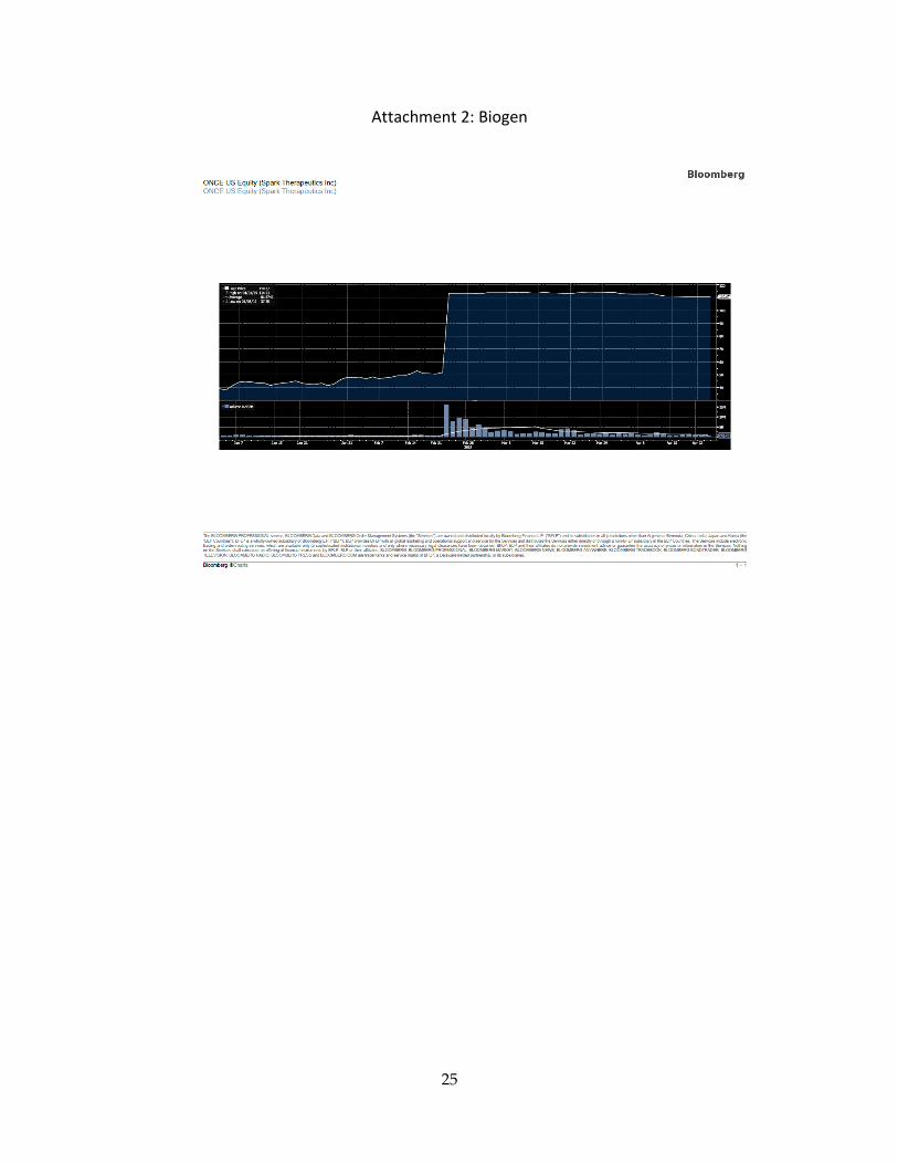
drug (see Attachment 1). A failure, however, can be catastrophic. Biogen, a large

pharmaceutical company saw its market capitalization1 fall by over a third (see Attachment 2) in

the March of 2019. Across both approval and rejection events, those who trade equities saw

the potential for massive gains.

The largest insider trading scandal in the history of the stock market surrounded a

biotechnology approval. Steven Cohen and his firm SAC Capital were long2 700 million dollars

on Elan, an Irish biotechnology company (Keefe 2017). Elan had submitted the most exciting

1 Market Capitalization- Value in totality of a company’s ownership shares outstanding 2 Long- to be long means to own and thus bet on the value of a company’s stock to rise.

3

Alzheimer’s drug of all time. Alzheimer’s has no cure and is famously difficult to treat. Bringing

a viable Alzheimer’s drug to market would be a veritable gold mine. When the firm

underhandedly learned of the drugs upcoming disappointing results, they not only liquidated,

but also reversed their position. They shorted3 the company’s stock, and made an illegal profit

of 275 million dollars (Keefe 2017).

A better understanding of the FDA approval process and the way a company’s stock

price fluctuates in the time surrounding approvals can yield practitioners a unique advantage in

their pursuit of profits. I hypothesize that biotechnology and pharmaceutical companies return

data surrounding Phase III FDA approvals will mimic the announcement effects traditionally

surrounding quarterly earnings. I also predict that less transparent firms will experience

greater cumulative abnormal returns, yielding negative and significant coefficients on all three

transparency measures: press releases one year prior to approval, analyst coverage, and the

cumulative abnormal return associated with the firm’s regular quarterly earnings

announcements.

The rest of the paper proceeds as follows: Section 2 provides a summary of the theory

and literature review, Section 3 describes the data, Section 4 analyzes the data and explains the

results, and Section 5 concludes.

2. Theory and Literature Review

The efficient market hypothesis states that markets are “efficient”, meaning that market

prices fully reflect all available information (Fama 1970). The price of a stock should reflect the

expected future value of the firm’s cash flows. In this framework, there are two types of risk:

3 Short- to short means to bet against, and thus yield profit when a company’s share price falls

4

unsystematic risk and systematic risk. Unsystematic risk, also known as specific risk, is the risk

associated with owning a specific security or investing in a specific industry. Imagine a

hypothetical individual whose entire portfolio consisted of one security, say Boeing. Given its

recent aircraft failures, Boeing saw a massive drop in stock price. Holding any one security

exposes the owner to that securities unsystematic risk. Imagine if rather than investing solely

in Boeing the hypothetical individual owned the stock of many companies in his portfolio. The

individual would be less exposed to the drop in Boeing’s stock price. The more stocks an

individual’s portfolio the lower the unsystematic risk of the portfolio. In an efficient market, all

unsystematic risk can be effectively eliminated via diversification. Systematic risk, also known

as market risk, is the uncertainty inherent in putting one’s money in the market. All stocks that

are traded are subject to changes in price when there are broad market movements. The

measure of a stock’s responsiveness to the market is called its beta. The risk of a portfolio can

be lowered to solely its systematic risk through diversification4.

This idea gave birth to capital asset pricing. Capital asset pricing theory aims to model

the expected returns of given securities. According to this theory because unsystematic risk

4

5

can be eliminated via portfolio construction, the only risk a shareholder must be compensated

for is systematic risk. By controlling for the factor of the market and adjusting for the current

risk-free rate of return5, it is possible to measure expected returns (Sharpe 1964). The first and

least restrictive model is the Market Model:

ri = rf + β1 (rm - rf)

ri : Expected Return on a given security rf : Risk-free rate rm : Return on the market

This model is able to predict the return on a specific security. This was the prevailing theory for

many years and by its virtue practitioners were able to create the security market line6 and

determine return for any given stock given its beta. The model had an issue, stocks were

earning return in excess of risk. Return in excess of predicted risk is called alpha6 and in an

efficient market this should not exist. Efficient market theorists believe that it is impossible to

beat the market and that any excess return must be due to some unseen risk.

5 The primary metric for estimating the risk free rate is the yield on 10 year treasury strips. Currently it is

approximately 2.5%. 6

6

In 1993 Eugene Fama and Kenneth French pioneered the Fama French Three Factor

Model:

ri = rf + β1 (rm - rf) + β2 (SMB) + β3 (HML) + ε

ri : Expected Return on a given security rf : Risk-free rate rm : Return on the market SMB: Size Premium, returns small cap minus large cap companies HML: book to market premium, High book to market minus low book to market

This model adds two new risk factors small minus big and high book to market minus low book

to market. This model assumes that smaller cap companies are inherently riskier than larger

cap companies and that companies with higher book to market are intrinsically less risky than

low book to market companies. This model controls for size and book to market value.

Proponents of the efficient market hypothesis argue that those factors represent risk factors

that must be accounted for when estimating the price of a stock (Fama 1993). Theoretically,

this variation of the CAPM should, with higher accuracy, predict the price of any given stock.

This model was the standard until it was updated to include a fourth factor for momentum:

ri = rf + β1 (rm - rf) + β2 (SMB) + β3 (HML) + β4 (Momentum) +ε

ri : Expected Return on a given security rf : Risk free rate rm : Return on the market SMB: Size Premium, returns small cap minus large cap companies HML: book to market premium, High book to market minus low book to market Momentum: Current trend upward or downward

7

Momentum describes the propensity of a company’s stock price to continue rising if it is going

up and to continue declining if it is going down. This is the final and most restrictive model.

Examining the difference between expected returns as predicted by these models and actual

daily returns yields a value for cumulative abnormal returns (CAR) (Brown 1985). The time

leading up to and surrounding an event yields robust data for the effect of that event on the

price of a security.

The efficient market hypothesis is widely accepted; however, some of its key

assumptions are not met when applied to Pharmaceutical and Biotechnology companies. In

order for efficiency to hold, not only must all knowledge be widely disseminated, but it also

must be scrutable to those who receive it. While much Pharmaceutical and Biotechnology data

is publicly available, it requires expert knowledge to understand, such that it is useless to the

general public due to information complexity (Janney 2003). This creates systematic

inefficiencies in the market due to the complexity of the information.

Not only private individuals fall victim to this knowledge gap; it is estimated that

anywhere from 35% to 40% of all publicly traded companies have no analysts assigned to cover

them. This dearth of coverage means that these innovative, high growth potential companies

are often not understood, even by institutional investors (Canviet 2010). This misalignment of

value is further driven by the ambiguity as to the effectiveness of the drug being developed and

the uncertainty of the FDA approval process. Many of these companies do not expect to have

cash flows of any kind for, in some cases, many years. Investments in this class of companies

are speculative and thus riddled with predictable irrational market behaviors. With a better

8

understanding of these market concepts, it is possible to net high abnormal returns in excess of

risk.

Examinations of announcement effects have long been examined in both finance and

economics literature. Early studies focused primarily on the impact of major financial

announcements like the establishment of a dividend or a firm’s regular quarterly earnings

announcements. One of the earliest papers that measured announcement effects associated

with earnings was published by William H. Beaver (1968). In his paper, he challenges Miller

and Modigliani’s (1963) assertions that firm announcements about earnings lack informational

value because there are often major measurement errors and other indicators convey firm

performance in a timelier manner. At the time, the prevailing wisdom was that the market

would have already processed that information and reflected it in its share price.

This assertion implies that earnings reports convey little the market does not already

know, and thus should not affect the price of a company’s securities. His data set included 143

firms traded on the New York Stock Exchange with a total of 506 earnings announcements. He

measured the stocks over a 17 week period surrounding the announcement with week t=0

being the week of the announcement and weeks t= -8 and t= +8 the eighth week directly

preceding and following, respectively. Beaver found that in week t=0 the volume of trading

increased, as did price volatility. This effect was coupled with decreased activity in weeks -8

through -1 and increased activity in week +1 through week +8. During week zero and the weeks

immediately following, the market violated “semi-strong efficiency” and abnormal returns were

realized. These types of abnormal returns surrounding earnings announcements have been

corroborated in both the United States and abroad and have remained congruent over time

9

(Landsman and Maydew 2002, Oopong 1995, Syed 2017). Similar results are also exhibited

surrounding announcements regarding dividends and special dividends across firms both

domestic and abroad (Dewentner 1998).

Financial disclosures are not the only important announcements for Pharmaceutical and

Biotechnology companies. FDA approval is an important step in the life cycle of these firms.

Rothenstien et. al (2011) examined the effect of Phase 3 FDA approval on the stock prices.

They examined 109 FDA trials and regulatory decisions. They found that the average price of a

stock in the 4-month period rose 13.7% prior to a positive release. Announcement effects are

seemingly present even before the announcement is made. Similar findings show that the

market largely overreacts post-release. Salil Sarkar and Pieter Jong (2006) find in an analysis of

189 firms that markets respond positively when the FDA approves a drug and negatively when

the FDA signals negatively. This effect has a greater magnitude for negative information. This

aligns with research on investor psychology (Wilcox 1998).

Similar results were noted by Thomas Hwang (2013) in a smaller data set of 24

regulatory decisions across all phases. His sample was primarily large U.S. Biotechnology

companies with drugs in the Oncology and Neurology space. Hwang found positive and

significant abnormal returns surrounding positives decisions and negative significant abnormal

within a two-day window of the event. His paper differed in that he found that abnormal

returns did not differ significantly by triall phase. Congruent with previous research, it was

determined that negative overreactions were of greater magnitude than positive overreactions.

Hwang’s assertions were corroborated by Anurag Sharma (2014), with a larger sample and a

longer event window of 21 days.

10

Transparency should lower cumulative abnormal returns. The efficient market

hypothesis states that market prices reflect all available information (Fama 1970). The more

information that is publicly available the more able the market should be to appropriately price

the stock. The more information put out by firm the more likely it is that the trading price will

reflect the true value. This decreases the likelihood of cumulative abnormal returns.

3. Data

The data for this study was collected from many sources. The sample consisted of 260

Phase III approvals from 150 companies from 2009 to 2018. To collect this data I gathered

approval dates and company names and stock tickers from the FDA Orange Book and

Biopharmcatalyst.com. With the dates and tickers, I was able to use the Wharton Data

Research services to pull the cumulative abnormal returns surrounding each approval. For this

estimation, the online research tool tracked the trading history of each company’s stock for 100

days to “estimate the expected return and residual return variance” (Wharton Research Data

Services). The sample consisted of companies with 70 valid trading days within this 100-day

window. The program uses a 50 trading day gap between the tracking period and the

estimation period. This limits the “likelihood that the risk model estimation is affected by the

event-induced return variance” (Wharton Research Data Services). For this study two

estimation windows were used, a three day window (one day prior to and one day after the

approval, which will be referred to as -1, +1) and a seven day window (three days prior to and

three days after the approval, which will be referred to as -3, +3). The data service then

automatically calculates the expected return using various asset pricing models. This paper will

focus on the least restrictive, the Market Model, and the most restrictive, the Fama French Plus

11

Momentum Model. Then the data service subtracts then subtracts the expected return from

the actual return experienced in the estimation window. This value is the cumulative abnormal

returns. I then took the absolute value of the Cumulative abnormal return to measure the

absolute degree of the change independent of direction and winsorized7 the highest five

percent of the sample

I used three variables as a proxy for transparency: company press release made within

the year to The Phase III announcement, number of analysts covering8 the stock at the time of

approval, and the absolute value of the average cumulative abnormal return surrounding the

four quarterly earnings announcements made prior to the Phase III announcement. The

Security and Exchange Commission mandates all publicly traded companies report both

quarterly (using a 10-K form) and yearly (using a 10-Q form) to report the status of the

business. Firms can opt to use a press release (using an 8-K) form to report additional

information. The more transparent the firm the greater number of 8-Ks it will file. I predicted

that the beta associated with press releases would be negative and significant.

I used the number of analyst covering a firm at the time of announcement. Coverage

Studies in the past have used this metric as a measure of information asymmetry9 (Chang

2006). There is strong evidence supporting the notion that the number of analysts covering a

firm is negatively correlated with the information asymmetry of a given firm (Chang 2006). The

7 Winsorize- to eliminate outliers and replace them with the observations closest to them (Hargrave 2018).

This is done to limit the effect of abnormal extreme values, or outliers, on the calculation (Hargrave 2018). 8 Analyst Coverage- A stock is covered when sell-side analyst publishes research reports and investment

recommendations for clients. 9 Information Asymmetry- information relating to a transaction in which one party has relevant

information that is not known by or available to the other party

12

more analyst covering a firm, the more information there should be available on that firm,

increasing transparency. This was collected using the Analyst recommendation function on

Bloomberg. This page displays research analysis from each analyst covering a firm. For each

company in the data set I counted the number of analysts that covered the stock on the

approval date. I predicted that the beta associated with analyst coverage would be negative

and significant.

The final metric used for transparency was the cumulative abnormal returns

surrounding a firms quarterly earnings announcements. These quarterly announcements often

contain major business updates. Large price reactions surrounding quarterly earning imply

reports that are highly informative. I hypothesized that the more information that exists about

a firm the more effectively it can be priced and thus the less likely you are to pick up cumulative

abnormal returns in the future surrounding the Phase III announcement. To collect this data I

used the COMPUSTAT data set and the previously gathered company tickers and found the

quarterly earnings announcement dates. Next, I ran 4 WRDS event studies for each earnings

announcement one year prior to approval. It was necessary to match the window of the

dependent variable to the window of the independent variable; as such, it was necessary to

have estimates for both window lengths across both models (Market and Fama French Plus

Momentum Model). Then, I averaged the absolute value of the four for a single cumulative

abnormal return value. All three transparency measures were winsorized.

From COMPUSTAT I also collected values for each company’s total assets, capital

expenditures, earnings per share, net income, operating income after depreciation, in-process

research and development, and sales, all of which were winsorized (see Table One for variable

13

names and descriptions). The average firm in the sample has $29.34 million in assets, $7.25

million in sales annually, and earns a net income of $1.29 million per year (See Table Two for

descriptive statistics on all key variables).

4. Results

Table Three is a correlation matrix for all key variables. The correlation matrix revealed

interesting significant correlations between the return variables and the transparency variables:

analyst coverage, press releases, and the cumulative abnormal returns surrounding earnings

announcements. I hypothesize that there would be significant and negative coefficients on all

transparency variables.

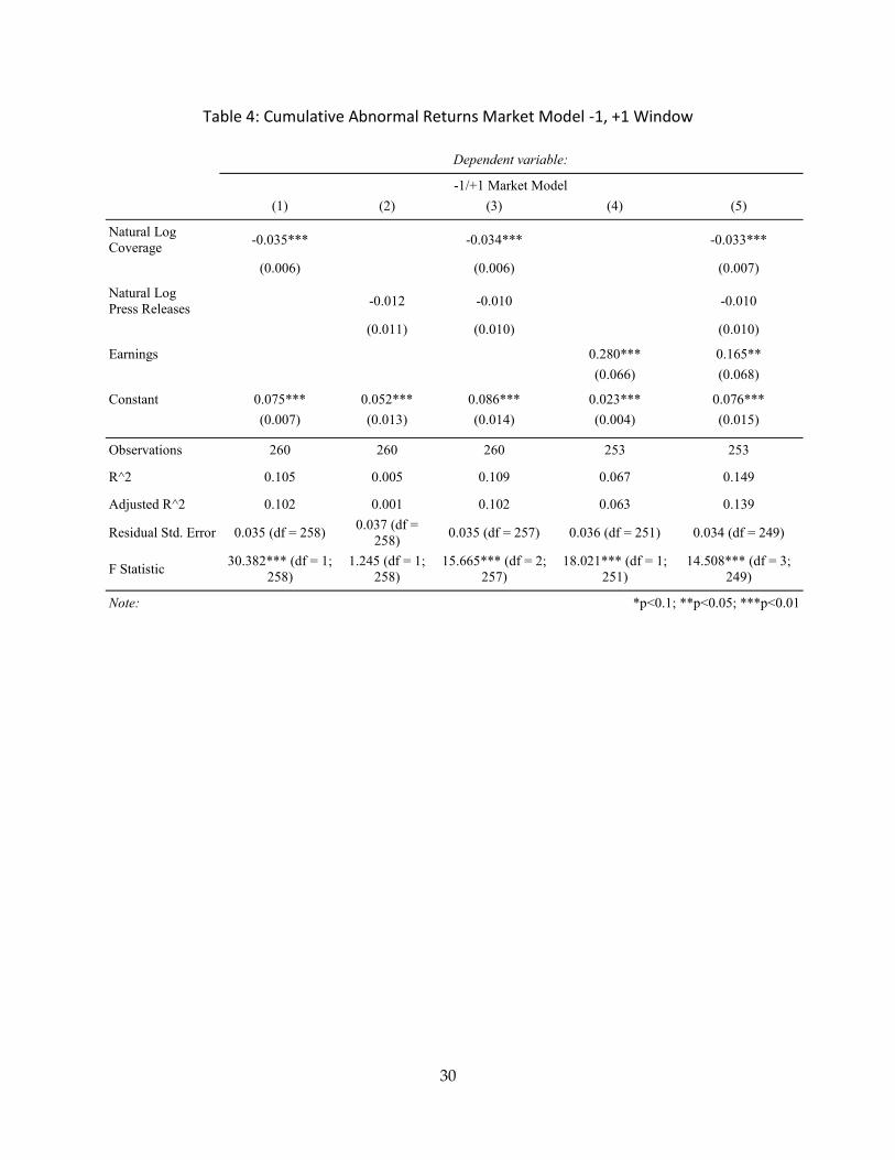
Table Four shows results of all OLS regressions using -1, +1 Market Model cumulative

abnormal returns. The first condition regressed Market Model cumulative abnormal returns

against the natural log of analyst coverage:

1) MM +1,-1 CAR = α+ β1 ( Ln Coverage ) + μ

This yielded a negative and significant beta value of -0.035 (p<0.01). This means that as analyst

coverage increases by one percent the cumulative abnormal returns should be lowered by

0.035%. While this may seem small in magnitude given the potentially large size of investments

an increased return of 0.035% can yield large monetary rewards in excess of risk. Then, I

regressed the same dependent variable against the natural log of press releases:

2) MM -1, +1 CAR = α+ β1 ( Ln 8-Ks ) + μ

This yielded a non-significant negative coefficient of -0.012 which is consistent with its

predicted direction. Next, I used both regressors in a combined test:

3) MM -1, +1 CAR = α+ β1 ( Ln Coverage ) + β2 ( Ln 8-Ks ) + μ

14

This yielded a -0.034 (p<0.01) beta for coverage and a negative non-significant beta of -0.010

for the number of press releases.

For robustness and to see if the effect diminished I extended the estimation window to -

3, +3 (see Table Five). Not only did the effect persist but it became more pronounced (Table

Four shows results of all OLS regressions using -3, +3 Market Model cumulative abnormal

returns). I first regressed the wider window Market Model cumulative abnormal returns

against the natural log of analyst coverage:

6) MM -3, +3 CAR = α+ β1 ( Ln Coverage ) + μ

The magnitude of the coefficient on coverage increased -0.056 (p<0.01). In this larger window,

a one percent increase in analyst coverage decreased cumulative abnormal returns by 0.056%.

Then, I regressed the same dependent variable against the natural log of press releases:

7) MM -3, +3 CAR = α+ β1 ( Ln 8-Ks ) + μ

Again this yielded a non-significant beta, -0.017, in the direction I predicted. Next, I ran a joint

test with both regressors:

8) MM -3, +3 CAR = α+ β1 ( Ln Coverage ) + β2 ( Ln 8-Ks ) + μ

This yielded a -0.055 (p<0.01) coefficient for coverage and a negative non-significant coefficient

of -0.014.

The Market Model is the least restrictive model. It is possible that the magnitude of the

cumulative abnormal return is lesser than is being predicted in my dependent variable and as

such all of my coefficients are inherently flawed. The Market Model does not control for known

risk factors such as company size, book to market ratio, or trends in stock prices. Companies

that are smaller are inherently riskier as are companies with high book to market ratios and

15

stock prices tend to demonstrate momentum in the short run. In an effort to assuage this

concern I ran the same analysis with the most restrictive model, the Fama French Plus

Momentum Model. Table Six shows results of all OLS regressions using -1, + Fama French Plus

Model cumulative abnormal returns.

In my first regression I regressed Fama French Plus Momentum Model cumulative

abnormal returns against the natural log of analyst coverage:

11) FFPM +1,-1 CAR = α+ β1 ( Ln Coverage ) + μ

This yielded a negative and significant beta value of -0.036 (p<0.01) greater in magnitude than

the Market Model. This means that a one percent change in analyst coverage lowers

cumulative abnormal returns by .036% Then, I regressed the same dependent variable against

the natural log of press releases:

12) FFPM -1, +1 CAR = α+ β1 ( Ln 8-Ks ) + μ

This yielded a non-significant negative coefficient of -0.012 the direction I predicted.

Next, I tested both regressors:

13) FFPM -1, +1 CAR = α+ β1 ( Ln Coverage ) + β2 ( Ln 8-Ks ) + μ

This yielded a -0.036 (p<0.01) beta for coverage and a negative non-significant beta of -0.010

for the number of press releases.

For robustness and again to see if the effect diminished I extended the estimation

window to -3, +3. Table Seven shows results of all OLS regressions using -3, +3 Fama French

Plus Momentum Model cumulative abnormal returns). In this condition I first regressed Fama

French Plus Momentum Model cumulative abnormal returns against the natural log of analyst

coverage:

16

16) FFPM -3, +3 CAR = α+ β1 ( Ln Coverage ) + μ

The magnitude of the coefficient on coverage again increased to -0.054 (p<0.01). In this larger

window, a one percent increase in analyst coverage decreased cumulative abnormal returns by

0.054%. Then, I regressed the same dependent variable against the natural log of press

releases:

17) FFPM -3, +3 CAR = α+ β1 ( Ln 8-Ks ) + μ

Again this yielded a non-significant beta, -0.021, in the direction I predicted. Next, I ran a

joint test with both regressors:

18) FFPM -3, +3 CAR = α+ β1 ( Ln Coverage ) + β2 ( Ln 8-Ks ) + μ

This yielded a -0.054 (p<.01) beta for coverage and a negative non-significant beta of -0.018 for

the number of press releases.

Next, I aimed to quantify the effect of cumulative abnormal returns surrounding

earnings announcements. I hypothesized that the beta would be significant and negative. It

was my expectation that more informative quarterly earnings would cause broad movements in

stock price, yielding cumulative abnormal returns surrounding these announcements. The

more information available in the market prior to the Phase III approval the more informative

the firm is and thus the lower cumulative abnormal surrounding the approval.

First, I used the least restrictive model, the Market Model, regressing Market Model

cumulative abnormal returns surrounding earnings announcement during the prior year against

cumulative abnormal returns surrounding Phase III approval (see Table Four):

4) MM -1, +1 CAR = α+ β1 ( CAR Earnings -1,+1 ) + μ

17

This yielded a positive significant beta of 0.280 (p<.01). This means that a one unit change in

cumulative abnormal returns surrounding earnings increased cumulative abnormal returns

surrounding approval by 0.280. For robustness increased the window to -3, +3 (see Table Five):

9) MM -3, +3 CAR = α+ β1 ( CAR Earnings -3, +3) + μ

This yielded a positive and significant coefficient of .379 (p<0.01).

Next, I moved to the Fama French Plus Momentum Model. I began by regressing the

Fama French Plus Momentum Model cumulative abnormal returns with a -1, +1 window against

cumulative abnormal returns surrounding Phase III approval (see Table Six):

14) FFPM -1, +1 CAR = α+ β1 ( CAR Earnings -1,+1 ) + μ

This yielded a positive significant beta of 0.283 (p<0.01). For robustness increased the window

to -3, +3 (see Table Seven):

19) FFPM -3, +3 CAR = α+ β1 ( CAR Earnings -3, +3) + μ

This yielded a positive and significant beta of 0.365 (p<0.01).

In all models across all windows the variable for cumulative abnormal returns

surrounding quarterly earnings announcements is added to the other transparency variables

the coefficient for coverage remains negative and significant (p<0.01) and the coefficient on

cumulative abnormal return surrounding earnings announcements remains positive and

significant (p<0.01), while both decrease in magnitude. The beta on Press Releases was always

negative and non-significant (see Tables Four, Five, Six, and Seven).

I next aimed to examine if there was a difference between firms that were highly

transparent and firms that were exceptionally tight-lipped. For the rest of my analysis, I used

only the -1, +1 day window cumulative abnormal returns from the Fama French Plus

Momentum Model. I broke down each of my key transparency variables into above and below

18

median (see Table Eight). Firms above median in press releases did not see significantly

different cumulative abnormal returns surrounding Phase III approval. Analyst coverage,

however, bore more interesting results. In both models there were significantly higher

cumulative abnormal returns for firms that were above median. In the Market Model, below

median analyst coverage firms averaged cumulative abnormal returns of 0.04892 and above

median firms returned only 0.02684 making the difference 0.02207. To test this difference, in

this condition and in all following conditions I used an independent sample T-test. This

difference was statistically significant with a p-value less than 0.01 (see table 8). The same

principle holds true in the more restrictive Fama French Plus Momentum Model, albeit with a

lower magnitude. Below median covered firms averaged cumulative abnormal of 0.04841 and

above median firms returned only 0.02690, making the difference .02151. This difference was

statistically significant with a p-value less than .01. The effect of cumulative abnormal returns

surrounding earnings produced opposite results. Above median firm in this category, using the

Market Model saw returns averaging at 0.04753, 0.01930 greater than below median firms

which saw returns of only 0.02824. The difference between the two groups was statistically

significant (p<.05). The same was true for the Fama French Plus Momentum Model (see Table

Eight).

Based on these results I created two new variables: the high transparency firm and the

low transparency firm (see Table Nine). In order to qualify as low transparency the firm had to

have below the median values for all three transparency measures, press releases, analyst

coverage, and cumulative abnormal returns surrounding earnings (see Table Nine). Conversely,

19

the high transparency firm was required to be above the median in all three categories. In my

sample there were 12 low transparency firms and 23 high transparency firms.

Both high and low transparency firms experienced cumulative abnormal returns

surrounding their Phase III announcement. The low transparency firms, on average, saw

Market Model cumulative abnormal returns of 0.08418 while the high transparency firms saw

cumulative abnormal returns of only 0.04868 a statistically significant difference (p<0.05). The

returns when the Fama French Plus Momentum Model was applied also had a statistically

significant difference (p<0.05). Low transparency firms had cumulative abnormal returns

0.07778 while high transparency firms saw returns of only 0.04759. When I added a dummy

variable for least transparent firm to the full Fama French Plus Momentum Model regression it

generated a positive and significant beta of 0.022 (p<0.05) (see Table Ten). This means that the

less transparent firms typically experience greater cumulative abnormal returns.

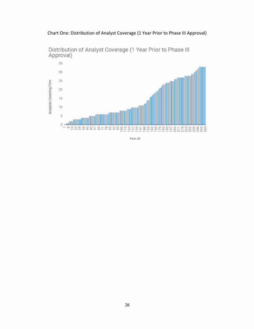
This led me to wonder if there was a nonlinear relationship between any of the

transparency measures and my cumulative abnormal return variables. First I ran a regression of

Fama French Plus Momentum Model -1, +1 cumulative abnormal returns against analyst

coverage and analyst coverage squared (see Table Eleven):

23) FFPM -1, +1 CAR = α+ β1 ( Ln Coverage ) + β2 ( Ln Coverage2 ) + μ

This yielded interesting results. The sign on the beta associated with coverage switched from

-0.036 (p<0.01) to 0.057 (p<0.05) and the beta on squared coverage was -0.047 (p<0.01). This

seemingly implies a non-linear relationship. After examining the relationship further the

maximum of the model peaks at firms with two covering analysts. Given that my sample has so

20

few examples of this I feel the relationship, while interesting and plausible, may be spurious

(see Chart One).

The final test I ran was an interaction between my analyst coverage variable and my

quarterly earnings cumulative abnormal returns with Fama French Plus Momentum Model -1,

+1 cumulative returns as the dependent variable:

24) FFPM -1, +1 CAR = α+ β1 ( Ln Coverage ) + β2 ( CAR Earnings -1,+1)

25) FFPM -1, +1 CAR = α+ β1 ( Ln Coverage ) + β2 ( CAR Earnings -1,+1) + β3 ( Ln Coverage* CAR

Earnings -1,+1) + μ

The first regression (without the interaction) bore coefficients of -0.035 on coverage (p<0.01)

and 0.0145 on earnings (p<0.05) (see Table Twelve). The regression with interaction term

yielded different results. The coverage beta increased in magnitude to -0.043 (p<0.01). The

beta on quarterly earnings cumulative abnormal returns flipped signs to -0.016 and lost its

significance. The interaction term had a non-significant beta of 0.155

5. Conclusions

Cumulative abnormal returns on company stocks exist from the least restrictive pricing

model (the Market Model) to the most restrictive generally accepted pricing model (the Fama

French Plus Momentum Model). The markets respond so positively that the returns subsist

from the -1, +1 window to the -3, +3 window.

My hypothesis surrounding analyst coverage rang true. Across all models and time

windows the beta associate with coverage remained significant and negative. Analyst coverage

acts as an effective proxy for transparency as both retail and institutional investors follow the

guidance of informed analysts. This effect is likely exacerbated, as analyst coverage is also a

21

proxy for general institutional awareness of the firm’s existence. When I examined my findings

surrounding a potential nonlinear relationship between coverage and cumulative abnormal

returns while potential spurious the data suggested that firms with two or less analyst covering

them at the time of approval saw positive returns to an increase in analyst coverage. My

sample, unfortunately, had too few examples of this class of company to derive meaningful

conclusions from this enhanced model. While my sample was limited in this way it did capture

the majority of Phase III approvals from 2009- 2018. Given this comprehensive makeup, I posit

that the dearth of firms with 0-2 analyst covering them was a function of the rarity of the

situation rather than a limitation of my sample. A firm that makes it through Phase I, and II and

into Phase III without gathering the attention of analyst, many of whom specialize by industry,

seems like a major oddity. An examination of these extremely under covered firms deserves

more attention. It may be necessary to extend the timeframe of the sample to gather sufficient

data.

While I was correct regarding the directionality of the beta associated with press

releases one year prior to approval across all models and windows this metric never yielded

significant data. It is possible that press releases are not an effective measure for transparency

because they can cover many different corporate events and announcements. A large number

of press releases released in a given year means that the firm is extremely communicative but

does not necessarily guarantee that the information released is substantive. A firm is required

to release an 8-K whenever it communicates material information10 to the public. The

definition of material is vague and as such can mean many different things. A firm may release

10 Any information about a company that may cause a change in the price of a share of its stock

22

an 8-K for anything a minor change in company bylaws, to a major change like the hiring or

firing of a key executive. Using the sheer number that a company releases may not be a viable

measure for transparency. Ideally, if there was a way to quantify the information content of

each individual press release on a scale from uninformative to highly informative that would

much improve the validity of the measure. I predict this may yield similar results to my findings

regarding analyst coverage.

My hypothesis surrounding cumulative abnormal returns surrounding earnings

announcements was incorrect. The beta with which it was associated was consistently positive

and significant (barring the interaction), the opposite of what I expected. Rather than

decreasing cumulative abnormal returns surrounding Phase III approval, firms with larger

cumulative abnormal returns surrounding earnings actually saw larger returns. I expected that

firms with greater quarterly cumulative abnormal returns had earnings reports that were

inherently more informative. The more information in the quarterly earnings report the

greater expected cumulative abnormal return surrounding the report should be. More

informative reports mean more information about the firm exists and the more effectively the

stock should be priced. These assumptions did not hold true. This area deserves more

attention.

This research helps illuminate a potential risk factor for which stock pricing methods

could be adjusted to increase their accuracy: transparency. While it is difficult to quantify firms

that have positive fundamentals but are less transparent have potential for excess returns. This

paper affirms that analyst coverage is an appropriate proxy for transparency and as such

absolute return managers may benefit from seeking out under covered companies.

23

There are also implications from a policy perspective. If efficiency and price discovery is

the goal of markets then pharmaceutical and biotechnology company’s deserve special

attention. Efficiency could through improved by the enforcement of a mechanism to either

mandate or encourage increased transparency from these types of firms. Increased

transparency would eliminate a good deal of randomness from stock selection and allow

institutions and retail investors to more effectively allocate their capital. Uncertainty decreases

the amount a person is willing to pay for something regardless of its inherent worth. The

market can more effectively price a good the more they understand about the good, whether it

be a real good or a financial one. Given the large potential cash inflows and high degree of

uncertainty from a Phase III drug approval announcements, all parties benefit from decreasing

this information asymmetry. Periodic data releases and potentially mandated incremental

reports to company shareholders should increase overall market efficiency. A more informed

market is a more efficient market, and this is especially true for the pharmaceutical and

biotechnology industry.

24

Attachment 1: Spark Therapeutics

25

Attachment 2: Biogen

26

Attachment 3: Visual Representation of Likelihood of Approval

Phase I:

Phase II:

Phase III:

= Denied

= Approved

27

Table 1: Variable Names and Descriptions

Variable Name Description

8Ks Press Releases (8Ks) 1 year prior to approval

Coverage # of Analyst Covering company at the announcement +1

Phase 3 Approval Anncmt.

Return: MM [-3,+3]

Absolute Value of Market Model Cumulative Abnormal Returns

Surrounding Phase 3 approvals [-3,+3]

Phase 3 Approval Anncmt.

Return: MM [-1,+1]

Absolute Value of Market Model Cumulative Abnormal Returns

Surrounding Phase 3 approvals [-1,+1]

Phase 3 Approval Anncmt.

Return: FFPM [-3,+3]

Absolute Value of Fama French Plus Mometum Cumulative

Abnormal Returns Surrounding Phase 3 approvals [-3,+3]

Phase 3 Approval Anncmt.

Return:FFPM [-1,+1]

Absolute Value of Fama French Plus Mometum Cumulative

Abnormal Returns Surrounding Phase 3 approvals [-1,+1]

Ln8ks Natural Log of Press Releases (8Ks) 1 year prior to approval + 1

LnCoverageNatural Log of # of Analyst Covering company at the

announcement +1

Total Assets Total Assets

CAPEX Capital Expenditures

EPS EPS Diluted Including Extraordinary Items

Net Income Net Income

Operating Income Operating Income After Depreciation

R+D In Process R+D

Sales Sales

Earnings Anncmt. Return:

MM [-1,+1]

Average Absolute Value of Market Model Cumulative Abnormal

Returns Surrounding Quarterly Earnings Announcement [-1,+1]

Earnings Anncmt. Return:

MM [-3,+3]

Average Absolute Value of Market Model Cumulative Abnormal

Returns Surrounding Quarterly Earnings Announcement [-3,+3]

Earnings Anncmt. Return:

FFPM [-1,+1]

Average Absolute Value of Fama French Plus Mometum

Cumulative Abnormal Returns Surrounding Quarterly Earnings

Announcement [-1,+1]

Earnings Anncmt. Return:

FFPM [-3,+3]

Average Absolute Value of Fama French Plus Mometum

Cumulative Abnormal Returns Surrounding Quarterly Earnings

Announcement [-3,+3]

Table One: Variable Names and Descriptions

28

Table 2: Descriptive Statistics

Transparency: N Mean Median StandardDeviation 25% 75% Min MaxPressReleases(8Ks)1yearpriortoapproval 260 16.5769 14 10.5156 10.25 18 2 52

#ofAnalystCoveringcompanyattheapproval+1 260 14.2115 10 10.2172 6 25 0 33

NaturalLogofPressReleases(8Ks)1yearpriortoapproval+1

260 1.1887 1.1761 0.2111 1.0508 1.2788 0.4771 1.7243

NaturalLogof#ofAnalystCoveringcompanyatthe

approval+1260 1.0636 1.0414 0.3454 0.8451 1.4150 0.0000 1.5315

ReturnsSurroundingPhaseIIIApproval: N Mean Median StandardDeviation 25% 75% Min Max

AbsoluteValueofMarketModelCumulativeAbnormalReturnsSurroundingPhase3approvals[-

3,+3]

260 0.0559 0.0390 0.0530 0.0145 0.0786 0.0001 0.1824

AbsoluteValueofMarketModelCumulative

AbnormalReturnsSurroundingPhase3approvals[-

1,+1]

260 0.0379 0.0250 0.0367 0.0097 0.0549 0.0000 0.1298

AbsoluteValueofFamaFrenchPlusMomentum

CumulativeAbnormalReturnsSurroundingPhase3approvals[-3,+3]

260 0.0574 0.0381 0.0552 0.0136 0.0832 0.0002 0.1822

AbsoluteValueofFamaFrenchPlusMomentumCumulativeAbnormalReturnsSurroundingPhase3

approvals[-1,+1]

260 0.0377 0.0249 0.0359 0.0091 0.0572 0.0000 0.1225

ReturnsSurroundingQuarterlyEarnings

Announcements:N Mean Median StandardDeviation 25% 75% Min Max

AverageAbsoluteValueofMarketModelCumulative

AbnormalReturnsSurroundingQuarterlyEarnings

Announcement[-1,+1]

253 0.0556 0.0490 0.0342 0.0302 0.0735 0.0038 0.1409

AverageAbsoluteValueofMarketModelCumulativeAbnormalReturnsSurroundingQuarterlyEarnings

Announcement[-3,+3]

253 0.0748 0.0602 0.0453 0.0405 0.1006 0.0119 0.1822

AverageAbsoluteValueofFamaFrenchPlus

MomentumCumulativeAbnormalReturns

SurroundingQuarterlyEarningsAnnouncement[-

1,+1]

253 0.0548 0.0447 0.0333 0.0282 0.0734 0.0024 0.1340

AverageAbsoluteValueofFamaFrenchPlus

MomentumCumulativeAbnormalReturns

SurroundingQuarterlyEarningsAnnouncement[-

3,+3]

253 0.0745 0.0611 0.0481 0.0366 0.1014 0.0110 0.1909

FinancialControlVariables(inmillions): N Mean Median StandardDeviation 25% 75% Min Max

TotalAssets 254 29,336.10$ 390.88$ 47,771.68$ 102.16$ 51,536.00$ 3.64$ 152,807.00$

CapitalExpenditures 254 264.91$ 3.31$ 446.35$ 0.17$ 398.18$ -$ 1,533.00$

EPSDilutedIncludingExtraordinaryItems 256 0.08-$ 0.31-$ 2.16$ 1.07-$ 1.14$ 8.51-$ 4.37$

NetIncome 256 1,292.68$ 12.98-$ 2,643.72$ 48.33-$ 1,416.18$ 5,325.00-$ 8,719.00$OperaingIncomeAfterDepreciation 255 1,927.95$ 10.12-$ 3,381.97$ 42.47-$ 3,133.00$ 445.74-$ 11,041.00$

InProcesssR+D 256 27.73$ -$ 82.74$ -$ -$ -$ 343.00$

Sales 256 7,245.57$ 37.15$ 11,842.35$ 0.80$ 12,757.75$ -$ 38,843.00$

Table2:Descriptives

29

Table 3: Correlation Matrix

eightkcoverag

e

abs_thre

e_mm_c

ar

abs_one

_mm_ca

r

abs_thre

e_ffpm_c

ar

abs_one

_ffpm_ca

r

leightklcoverag

eATQ CAPXY EPSFIY NIY OIADPY RDIPY SALEY

Earnings

Anncmt.

Return: MM

[-1,+1]

Earnings

Anncmt.

Return: MM

[-3,+3]

Earnings

Anncmt.

Return:

FFPM [-1,+1]

Earnings

Anncmt.

Return: FFPM

[-3,+3]

1 -0.01231 0.00313 -0.00133 0.02241 -0.00106 1 -0.01231 0.08461 0.03228 -0.12479 -0.12537 -0.13495 -0.22107 0.06363 -0.00254 -0.00446 -0.01468 0.0058

0.8434 0.9599 0.983 0.7191 0.9864 <.0001 0.8434 0.1789 0.6086 0.0461 0.0451 0.0312 0.0004 0.3105 0.968 0.9437 0.8162 0.9269

-0.01231 1 -0.38974 -0.40156 -0.37631 -0.39229 -0.01231 1 0.81944 0.76478 0.44881 0.33085 0.42035 0.4567 0.74989 -0.43079 -0.50372 -0.4602 -0.50507

0.8434 <.0001 <.0001 <.0001 <.0001 0.8434 <.0001 <.0001 <.0001 <.0001 <.0001 <.0001 <.0001 <.0001 <.0001 <.0001 <.0001 <.0001

0.00313 -0.38974 1 0.61073 0.81598 0.56741 0.00313 -0.38974 -0.51769 -0.48517 -0.40019 -0.38575 -0.43473 -0.30346 -0.50257 0.3643 0.4171 0.36348 0.43353

0.9599 <.0001 <.0001 <.0001 <.0001 0.9599 <.0001 <.0001 <.0001 <.0001 <.0001 <.0001 <.0001 <.0001 <.0001 <.0001 <.0001 <.0001

-0.00133 -0.40156 0.61073 1 0.56706 0.79619 -0.00133 -0.40156 -0.52042 -0.51124 -0.37632 -0.39109 -0.4366 -0.27216 -0.48262 0.39297 0.39661 0.39775 0.41504

0.983 <.0001 <.0001 <.0001 <.0001 0.983 <.0001 <.0001 <.0001 <.0001 <.0001 <.0001 <.0001 <.0001 <.0001 <.0001 <.0001 <.0001

0.02241 -0.37631 0.81598 0.56706 1 0.58626 0.02241 -0.37631 -0.50161 -0.47939 -0.42886 -0.43432 -0.49047 -0.28017 -0.50324 0.3773 0.38717 0.36695 0.39457

0.7191 <.0001 <.0001 <.0001 <.0001 0.7191 <.0001 <.0001 <.0001 <.0001 <.0001 <.0001 <.0001 <.0001 <.0001 <.0001 <.0001 <.0001

-0.00106 -0.39229 0.56741 0.79619 0.58626 1 -0.00106 -0.39229 -0.52674 -0.50897 -0.37104 -0.37464 -0.43664 -0.27366 -0.48905 0.32763 0.35509 0.35433 0.3998

0.9864 <.0001 <.0001 <.0001 <.0001 0.9864 <.0001 <.0001 <.0001 <.0001 <.0001 <.0001 <.0001 <.0001 <.0001 <.0001 <.0001 <.0001

1 -0.01231 0.00313 -0.00133 0.02241 -0.00106 1 -0.01231 0.08461 0.03228 -0.12479 -0.12537 -0.13495 -0.22107 0.06363 -0.00254 -0.00446 -0.01468 0.0058

<.0001 0.8434 0.9599 0.983 0.7191 0.9864 0.8434 0.1789 0.6086 0.0461 0.0451 0.0312 0.0004 0.3105 0.968 0.9437 0.8162 0.9269

-0.01231 1 -0.38974 -0.40156 -0.37631 -0.39229 -0.01231 1 0.81944 0.76478 0.44881 0.33085 0.42035 0.4567 0.74989 -0.43079 -0.50372 -0.4602 -0.50507

0.8434 <.0001 <.0001 <.0001 <.0001 <.0001 0.8434 <.0001 <.0001 <.0001 <.0001 <.0001 <.0001 <.0001 <.0001 <.0001 <.0001 <.0001

0.08461 0.81944 -0.51769 -0.52042 -0.50161 -0.52674 0.08461 0.81944 1 0.92699 0.5736 0.49571 0.56468 0.42023 0.91393 -0.54001 -0.6372 -0.57328 -0.64676

0.1789 <.0001 <.0001 <.0001 <.0001 <.0001 0.1789 <.0001 <.0001 <.0001 <.0001 <.0001 <.0001 <.0001 <.0001 <.0001 <.0001 <.0001

0.03228 0.76478 -0.48517 -0.51124 -0.47939 -0.50897 0.03228 0.76478 0.92699 1 0.58628 0.49948 0.57998 0.42605 0.90807 -0.51219 -0.6281 -0.54639 -0.62993

0.6086 <.0001 <.0001 <.0001 <.0001 <.0001 0.6086 <.0001 <.0001 <.0001 <.0001 <.0001 <.0001 <.0001 <.0001 <.0001 <.0001 <.0001

-0.12479 0.44881 -0.40019 -0.37632 -0.42886 -0.37104 -0.12479 0.44881 0.5736 0.58628 1 0.88714 0.84867 0.2996 0.67172 -0.49542 -0.51946 -0.50468 -0.50658

0.0461 <.0001 <.0001 <.0001 <.0001 <.0001 0.0461 <.0001 <.0001 <.0001 <.0001 <.0001 <.0001 <.0001 <.0001 <.0001 <.0001 <.0001

-0.12537 0.33085 -0.38575 -0.39109 -0.43432 -0.37464 -0.12537 0.33085 0.49571 0.49948 0.88714 1 0.9091 0.2049 0.56557 -0.53749 -0.50632 -0.50517 -0.47271

0.0451 <.0001 <.0001 <.0001 <.0001 <.0001 0.0451 <.0001 <.0001 <.0001 <.0001 <.0001 0.001 <.0001 <.0001 <.0001 <.0001 <.0001

-0.13495 0.42035 -0.43473 -0.4366 -0.49047 -0.43664 -0.13495 0.42035 0.56468 0.57998 0.84867 0.9091 1 0.36361 0.64609 -0.55066 -0.52816 -0.51227 -0.49278

0.0312 <.0001 <.0001 <.0001 <.0001 <.0001 0.0312 <.0001 <.0001 <.0001 <.0001 <.0001 <.0001 <.0001 <.0001 <.0001 <.0001 <.0001

-0.22107 0.4567 -0.30346 -0.27216 -0.28017 -0.27366 -0.22107 0.4567 0.42023 0.42605 0.2996 0.2049 0.36361 1 0.44566 -0.27738 -0.35163 -0.28684 -0.35212

0.0004 <.0001 <.0001 <.0001 <.0001 <.0001 0.0004 <.0001 <.0001 <.0001 <.0001 0.001 <.0001 <.0001 <.0001 <.0001 <.0001 <.0001

0.06363 0.74989 -0.50257 -0.48262 -0.50324 -0.48905 0.06363 0.74989 0.91393 0.90807 0.67172 0.56557 0.64609 0.44566 1 -0.5156 -0.64784 -0.55089 -0.65671

0.3105 <.0001 <.0001 <.0001 <.0001 <.0001 0.3105 <.0001 <.0001 <.0001 <.0001 <.0001 <.0001 <.0001 <.0001 <.0001 <.0001 <.0001

-0.00254 -0.43079 0.3643 0.39297 0.3773 0.32763 -0.00254 -0.43079 -0.54001 -0.51219 -0.49542 -0.53749 -0.55066 -0.27738 -0.5156 1 0.77651 0.94756 0.74031

0.968 <.0001 <.0001 <.0001 <.0001 <.0001 0.968 <.0001 <.0001 <.0001 <.0001 <.0001 <.0001 <.0001 <.0001 <.0001 <.0001 <.0001

-0.00446 -0.50372 0.4171 0.39661 0.38717 0.35509 -0.00446 -0.50372 -0.6372 -0.6281 -0.51946 -0.50632 -0.52816 -0.35163 -0.64784 0.77651 1 0.77057 0.94374

0.9437 <.0001 <.0001 <.0001 <.0001 <.0001 0.9437 <.0001 <.0001 <.0001 <.0001 <.0001 <.0001 <.0001 <.0001 <.0001 <.0001 <.0001

-0.01468 -0.4602 0.36348 0.39775 0.36695 0.35433 -0.01468 -0.4602 -0.57328 -0.54639 -0.50468 -0.50517 -0.51227 -0.28684 -0.55089 0.94756 0.77057 1 0.78019

0.8162 <.0001 <.0001 <.0001 <.0001 <.0001 0.8162 <.0001 <.0001 <.0001 <.0001 <.0001 <.0001 <.0001 <.0001 <.0001 <.0001 <.0001

0.0058 -0.50507 0.43353 0.41504 0.39457 0.3998 0.0058 -0.50507 -0.64676 -0.62993 -0.50658 -0.47271 -0.49278 -0.35212 -0.65671 0.74031 0.94374 0.78019 1

0.9269 <.0001 <.0001 <.0001 <.0001 <.0001 0.9269 <.0001 <.0001 <.0001 <.0001 <.0001 <.0001 <.0001 <.0001 <.0001 <.0001 <.0001

ATQ

eightk

coverage

abs_three_mm_ca

r

Spearman Correlation Coefficients

Prob > |r| under H0: Rho=0

abs_one_mm_car

abs_three_ffpm_ca

r

abs_one_ffpm_car

leightk

lcoverage

Earnings Anncmt.

Return: MM [-

1,+1]

Earnings Anncmt.

Return: MM [-

3,+3]

Earnings Anncmt.

Return: FFPM [-

1,+1

Earnings Anncmt.

Return: FFPM [-

3,+3]

CAPXY

EPSFIY

NIY

OIADPY

RDIPY

SALEY

30

Table 4: Cumulative Abnormal Returns Market Model -1, +1 Window

Dependent variable:

-1/+1 Market Model

(1) (2) (3) (4) (5)

Natural Log

Coverage -0.035*** -0.034*** -0.033***

(0.006) (0.006) (0.007)

Natural Log

Press Releases -0.012 -0.010 -0.010

(0.011) (0.010) (0.010)

Earnings 0.280*** 0.165** (0.066) (0.068)

Constant 0.075*** 0.052*** 0.086*** 0.023*** 0.076*** (0.007) (0.013) (0.014) (0.004) (0.015)

Observations 260 260 260 253 253

R^2 0.105 0.005 0.109 0.067 0.149

Adjusted R^2 0.102 0.001 0.102 0.063 0.139

Residual Std. Error 0.035 (df = 258) 0.037 (df =

258) 0.035 (df = 257) 0.036 (df = 251) 0.034 (df = 249)

F Statistic 30.382*** (df = 1;

258)

1.245 (df = 1;

258)

15.665*** (df = 2;

257)

18.021*** (df = 1;

251)

14.508*** (df = 3;

249)

Note: *p<0.1; **p<0.05; ***p<0.01

31

Table 5: Cumulative Abnormal Returns Market Model -3, +3 Window

Dependent variable:

-3/+3 Market Model

(6) (7) (8) (9) (10)

Natural Log

Coverage -0.056*** -0.055*** -0.050***

(0.009) (0.009) (0.010)

Natural Log

Press Releases -0.017 -0.014 -0.013

(0.016) (0.015) (0.014)

Earnings 0.379*** 0.209***

(0.070) (0.076)

Constant 0.115*** 0.077*** 0.132*** 0.028*** 0.109*** (0.010) (0.019) (0.020) (0.006) (0.023)

Observations 260 260 260 253 253

R^2 0.132 0.005 0.135 0.104 0.185

Adjusted R^2 0.129 0.001 0.129 0.100 0.175

Residual Std. Error 0.049 (df = 258) 0.053 (df =

258) 0.049 (df = 257) 0.051 (df = 251) 0.048 (df = 249)

F Statistic 39.348*** (df = 1;

258)

1.240 (df = 1;

258)

20.134*** (df = 2;

257)

28.985*** (df = 1;

251)

18.809*** (df = 3;

249)

Note: *p<0.1; **p<0.05; ***p<0.01

32

Table 6: Cumulative Abnormal Returns Fama French Plus Momentum Model -1, +1 Window

Dependent variable:

-1/+1 Fama French Plus Momentum (11) (12) (13) (14) (15)

Natural Log

Coverage -0.036*** -0.036*** -0.035***

(0.006) (0.006) (0.007)

Natural Log

Press Releases -0.012 -0.010 -0.010

(0.011) (0.010) (0.010)

Earnings 0.283*** 0.142** (0.066) (0.069)

Constant 0.076*** 0.052*** 0.088*** 0.023*** 0.079*** (0.007) (0.013) (0.013) (0.004) (0.015)

Observations 260 260 260 253 253

R^2 0.123 0.005 0.126 0.068 0.160

Adjusted R^2 0.119 0.001 0.119 0.064 0.150

Residual Std.

Error 0.034 (df = 258) 0.036 (df = 258) 0.034 (df = 257) 0.035 (df = 251) 0.033 (df = 249)

F Statistic 36.030*** (df =

1; 258) 1.278 (df = 1; 258) 18.499*** (df = 2; 257)

18.251*** (df =

1; 251)

15.776*** (df =

3; 249)

Note: *p<0.1; **p<0.05; ***p<0.01

33

Table 7: Cumulative Abnormal Returns Fama French Plus Momentum Model -3, +3 Window

Dependent variable:

-3/+3 Fama French Plus Momentum

(16) (17) (18) (19) (20)

Natural Log

Coverage -0.054 *** -0.054 *** -0.046 ***

(0.009) (0.009) (0.011)

Natural Log

Press Releases -0.021 -0.018 -0.017

(0.016) (0.015) (0.015)

Earnings 0.365 *** 0.212 ***

(0.069) (0.076)

Constant 0.115 *** 0.082 *** 0.136 *** 0.031 *** 0.112 ***

(0.010) (0.020) (0.021) (0.006) (0.024)

Observations 260 260 260 253 253

R^2 0.115 0.006 0.119 0.099 0.166

Adjusted R^2 0.111 0.003 0.113 0.096 0.156

Residual Std.

Error 0.052 (df = 258)

0.055 (df =

258) 0.052 (df = 257) 0.053 (df = 251) 0.051 (df = 249)

F Statistic 33.482 *** (df = 1;

258)

1.671 (df = 1;

258)

17.436 *** (df = 2;

257)

27.629 *** (df = 1;

251)

16.530 *** (df = 3;

249)

Note: *p <0.1; **p <0.05; ***p <0.01

34

Table 8: Above and Below Median Transparency

Press Releases (8Ks) 1 year prior to approval Below Median Above Median Difference P Value

Phase 3 Approval Anncmt.

Return: MM [-1,+1]0.03698 0.03879 0.00180 0.69290

Phase 3 Approval Anncmt.

Return:FFPM [-1,+1]0.03650 0.03881 0.00232 0.60397

# of Analyst Covering company at the annoucement Below Median Above Median Difference P Value

Phase 3 Approval Anncmt.

Return: MM [-1,+1]0.04892 0.02685 -0.02207 7.60094E-07

Phase 3 Approval Anncmt.

Return:FFPM [-1,+1]0.04841 0.02690 -0.02151 8.27861E-07

Earnings Anncmt. Return: MM [-1,+1] Below Median Above Median Difference P Value

Phase 3 Approval Anncmt.

Return: MM [-1,+1]0.02824 0.04753 0.01930 1.71553E-05

Earnings Anncmt. Return: FFPM [-1,+1] Below Median Above Median Difference P Value

Phase 3 Approval Anncmt.

Return:FFPM [-1,+1]0.02869 0.04662 0.01793 4.54536E-05

Table 8 Breakdown Above and Below Median

35

Table 9: Most Versus Least Transparent Firms

Most Vs. Least Transparent

Model High Transparency Low Transparency Difference P-Value

Phase 3 Approval Anncmt. Return: MM [-1,+1]

0.04868 0.08418 -0.03550 0.03869

Phase 3 Approval Anncmt. Return:FFPM [-1,+1]

0.04759 0.07778 -0.03019 0.04306

36

Table 10: Cumulative Abnormal Returns Fama French Plus Momentum Model -1, +1 Window

with Dummy Variable for Least Transparent:

Dependent variable:

-1/+1 Fama French Plus Momentum

(21)

Natural Log Coverage -0.003 (0.010)

Natural Log

Press Releases -0.029***

(0.007)

Earnings 0.179** (0.070)

Least Transparent 0.022** (0.011)

Constant 0.063*** (0.017)

Observations 252

R^2 0.171

Adjusted R^2 0.158

Residual Std. Error 0.033 (df = 247)

F Statistic 12.745*** (df = 4; 247)

Note: *p<0.1; **p<0.05; ***p<0.01

37

Table 11: Fama French Plus Momentum Model Nonlinear Coverage

Dependent variable:

-1/+1 Fama French Plus Momentum (22) (23)

Natural Log

Coverage -0.036*** 0.057**

(0.006) (0.029)

Natural Log

Coverage Squared -0.047***

(0.014)

Constant 0.076*** 0.036*** (0.007) (0.014)

Observations 260 260

R2 0.123 0.158

Adjusted R2 0.119 0.152

Residual Std. Error 0.034 (df = 258) 0.033 (df = 257)

F Statistic 36.030*** (df = 1; 258) 24.177*** (df = 2; 257)

Note: *p<0.1; **p<0.05; ***p<0.01

38

Chart One: Distribution of Analyst Coverage (1 Year Prior to Phase III Approval)

39

Table 12: Fama French Plus Momentum Model Coverage and Earnings Interaction

Dependent variable:

-1/+1 Fama French Plus Momentum (24) (25)

Natural Log

Coverage -0.035*** -0.043***

(0.007) (0.012)

Earnings 0.145** -0.016 (0.069) (0.222)

Interaction 0.155 (0.202)

Constant 0.067*** 0.076*** (0.010) (0.015)

Observations 253 253

R^2 0.156 0.158

Adjusted R^2 0.150 0.148

Residual Std. Error 0.033 (df = 250) 0.033 (df = 249)

F Statistic 23.150*** (df = 2; 250) 15.602*** (df = 3; 249)

Note: *p<0.1; **p<0.05; ***p<0.01

40

Works Cited

Brown, Stephen J., and Jerold B. Warner. “Using Daily Stock Returns.” Journal of Financial

Economics, vol. 14, no. 1, 1985, pp. 3–31., doi:10.1016/0304-405x(85)90042.

Bloomberg L.P. Stock Price graph for Biogen. 12/1/19 to 04/24/19. Bloomberg terminal, 24 April

2019.

Bloomberg L.P. Stock Price graph for Spark Therapeutics. 12/1/19 to 04/24/19. Bloomberg

terminal, 24 April 2019.

Chang, Xin, et al. “Analyst Coverage and Financing Decisions.” The Journal of Finance, vol. 61,

no. 6, Dec. 2006, doi:10.2139/ssrn.571065.

Compustat Industrial [Annual Data]. 2009 to 2018. Available: Standard & Poor's/Compustat

04/24/19. Retrieved from Wharton Research Data Service.

CRSP Stocks. 2009 to 2018. Available: Center For Research in Security Prices. Graduate School

of Business. University of Chicago 04/24/19. Retrieved from Wharton Research Data

Service.

Dewenter, Kathryn L., and Vincent A. Warther. “Dividends, Asymmetric Information, and

Agency Conflicts: Evidence from a Comparison of the Dividend Policies of Japanese

and U.S. Firms.” The Journal of Finance, vol. 53, no. 3, 1998, pp. 879–904.,

doi:10.1111/0022-1082.00038.

Dimasi, Joseph A., et al. “Innovation in the Pharmaceutical Industry: New Estimates of R&D

Costs.” Journal of Health Economics, vol. 47, 2016, pp. 20–33.,

doi:10.1016/j.jhealeco.2016.01.012.

41

Fama, Eugene F. “Efficient Capital Markets: A Review of Theory and Empirical Work.” The

Journal of Finance, vol. 25, no. 2, 1970, p. 383., doi:10.2307/2325486.

Fama, Eugene F., and Kenneth R. French. “Common Risk Factors in the Returns on Stocks

and Bonds.” Journal of Financial Economics, vol. 33, no. 1, 1993, pp. 3–56.,

doi:10.1016/0304-405x(93)90023-5.

Hargrave, Marshall. “How to Use the Winsorized Mean.” Investopedia, Investopedia, 17 Apr.

2019, www.investopedia.com/terms/w/winsorized_mean.asp.

Hwang, Thomas J. “Stock Market Returns and Clinical Trial Results of Investigational

Compounds: An Event Study Analysis of Large Biopharmaceutical Companies.” PLoS

ONE, vol. 8, no. 8, July 2013, doi:10.1371/journal.pone.0071966.

Keefe, Patrick Radden. “Inside the Biggest-Ever Hedge-Fund Scandal.” The New Yorker, The New

Yorker, 19 June 2017, www.newyorker.com/magazine/2014/10/13/empire-edge.

Landsman, Wayne R., and Edward L. Maydew. “Beaver (1968) Revisited: Has the

Information Content of Annual Earnings Announcements Declined in the Past Three

Decades?” SSRN Electronic Journal, 2000, doi:10.2139/ssrn.204068.

Office of the Commissioner. “The Drug Development Process - Step 3: Clinical Research.” U S

Food and Drug Administration Home Page, Office of the Commissioner,

www.fda.gov/forpatients/approvals/drugs/ucm405622.htm.

Opong, Kwaku K. “The Information Content Of Interim Financial Reports: Uk Evidence.” Journal

of Business Finance & Accounting, vol. 22, no. 2, 1995, pp. 269–279.,

doi:10.1111/j.1468-5957.1995.tb00683.x.

42

Picardo, Elvis. “Phase 3.” Investopedia, Investopedia, 1 June 2018,

www.investopedia.com/terms/p/phase-3.asp.

Rothenstein, Jeffrey M., et al. “Company Stock Prices Before and After Public

Announcements Related to Oncology Drugs.” JNCI: Journal of the National Cancer

Institute, vol. 103, no. 20, 2011, pp. 1507–1512., doi:10.1093/jnci/djr338.

Sarkar, Salil K., and Pieter J. De Jong. “Market Response to FDA Announcements.” The

Quarterly Review of Economics and Finance, vol. 46, no. 4, 2006, pp. 586–597.,

doi:10.1016/j.qref.2005.01.003.

Sharma, Anurag, and Nelson Lacey. “Linking Product Development Outcomes to Market

Valuation of the Firm: The Case of the U.S. Pharmaceutical Industry*.” Journal of

Product Innovation Management, vol. 21, no. 5, 2004, pp. 297–308.,

doi:10.1111/j.0737-6782.2004.00084.x.

Sharpe, William F. “Capital Asset Prices: A Theory of Market Equilibrium under Conditions

of Risk.” The Journal of Finance, vol. 19, no. 3, 1964, p. 425., doi:10.2307/2977928.

Small Cap Analyst Coverage: An ‘Under-the-Radar’ Dilemma” World Federation of

Exchanges, 2010.

Syed, Ali Murad, and Ishtiaq Ahmad Bajwa. “Earnings Announcements, Stock Price Reaction

and Market Efficiency – the Case of Saudi Arabia.” International Journal of Islamic

and Middle Eastern Finance and Management, vol. 11, no. 3, 2018, pp. 416–431.,

doi:10.1108/imefm-02-2017-0044.

Wharton Research Data Services. , 1993. Internet resource.

43

Wilcox, Stephen E. “Investor Psychology and Security Market Under- and Overreactions.”

CFA Digest, vol. 29, no. 2, 1999, pp. 69–71., doi:10.2469/dig.v29.n2.480.