Office of Tax Analysis

Working Paper 111

November 2016

Have Excess Returns To Corporations Been Increasing

Over Time?

Laura Power & Austin Frerick

The OTA Working Papers Series presents original research by the staff of the Office of Tax

Analysis. These papers are intended to generate discussion and critical comment while

informing and improving the quality of the analysis conducted by the Office. The papers are

works in progress and subject to revision. Views and opinions expressed are those of the authors

and do not necessarily represent official Treasury positions or policy. Comments are welcome,

as are suggestions for improvements, and should be directed to the authors. OTA Working

Papers may be quoted without additional permission.

2

HAVE EXCESS RETURNS TO CORPORATIONS BEEN INCREASING OVER

TIME?

November 2016

Laura Power1 & Austin Frerick

2

This paper examines the difference between a corporate income tax base and a corporate

consumption tax base over time. Using a micro-data panel of tax returns of C corporations from

1992 to 2013, we estimate the fraction of the tax base attributable to the risk-free return in each

year, and show that it has gradually declined over time, averaging 40 percent from 1992–2002 and

25 percent from 2003–2013. This decrease means that the difference between an income tax base

and a consumption tax base has also declined, and suggests that “excess” returns are becoming

more important to the tax base.

Keywords: Excess Returns, Risk-free Returns, Cash Flow Tax

JEL Codes: H25 and H22

1 Laura Power: Office of Tax Analysis, U.S. Department of the Treasury, Laura.Power@treasury.gov.

2 Austin Frerick: Office of Tax Analysis, U.S. Department of the Treasury, Austin.Frerick@treasury.gov.

3

I. INTRODUCTION

Have excess returns to corporations been increasing over time? Our evidence suggests that

they have. The distinction among types of returns to capital (e.g.; risk-free, risk adjusted, windfalls

attributable to good luck, etc.) frequently arises in economic theory and policy, and several

researches have attempted to measure these different types of returns (Auerbach (1993), Gentry and

Hubbard (1997), and Toder and Reuben (2005)). The risk-free return is particularly relevant for tax

policy formulation, because the risk-free return is treated differently under an income tax than under

a consumption tax. Specifically, an income tax includes the risk-free return to capital in the tax

base, thereby distorting taxpayers’ decisions, whereas a consumption tax does not.3 If the majority

of the current tax base is attributable to returns in excess of the risk-free rate, then the difference

between a consumption tax base and the current income tax base is relatively small. This small

difference means that most of the current tax base would still be taxed under a consumption tax.

Further, if returns in excess of the risk-free rate have been increasing as a fraction of corporate

income, then the difference between the current income tax base and a consumption tax base has

been declining over time.

We begin with a brief literature review and then discuss our methodology for measuring the

risk-free return. Next, we present the results from applying that methodology separately for all C

corporations and multinational corporations (MNCs). Then, we present estimates of the risk-free

return by industry and explain the separate cases for the financial and real estate sectors. We also

discuss an alternative to the basic methodology for comparison. Finally, we conclude with the

implications of the results.

3 The U.S. income tax, which has incentives such as accelerated depreciation, is actually a hybrid between a pure

income tax and a consumption tax. Therefore, it already exempts part of the risk-free return from tax.

4

II. LITERATURE REVIEW

A variety of papers discuss and estimate the composition of an income tax base versus a

consumption tax base, as well as describe the distributional and revenue implications of these

different bases. Using 1989 stock market data, Gentry and Hubbard (1997) estimate that the risk-

free return is approximately 40 percent of the return to corporate capital. They categorize the

components of the corporate return into four categories: the marginal (risk-free) return, infra-

marginal returns (economic profits), the risk premium, and ex-post luck. They argue convincingly

that an income tax captures the marginal (risk-free) return, while a consumption tax does not, but

that both taxes treat all other types of returns the same. Therefore, in order to determine how the

relationship between a consumption tax base and an income tax base has been changing over time,

we focus on measuring the risk-free return to capital. We refer to all returns in excess of this risk-

free rate (including returns to risk, entrepreneurial labor, decreasing returns to scale, market power,

luck, etc.) as excess returns.

Gordon and Slemrod (1988), Gentry and Hubbard (1997), and Toder and Rueben (2005), all

estimate the change in the tax base that results from changing the current tax system, which taxes

the risk-free return to capital, to a consumption tax system, which exempts the risk-free return to

capital. Because of the unique properties of the financial sector, they confine their analysis to the

nonfinancial sector. For 2004, Toder and Rueben (2005) estimate the ratio of this change to the

taxable income base is 32 percent. They attribute that fraction of the tax base to the normal return to

capital.4 Cronin et al. (2012) use a similar methodology and perform the estimates for five separate

years to obtain an average fraction of 37 percent.5

4 Cronin et al. (2012) provide a detailed literature review.

5 Cronin et al. (2012) include additional details regarding the distinction between the Toder and Reuben (2005)

methodology and their methodology.

5

III. METHODOLOGY

We refine the Cronin et al. (2012) methodology and extend the time horizon back 21 years in

order to determine how the fraction of the return attributable to the risk-free return changes over

time. We present an overview of the methodology here, while we report the details in Appendix A.

For our analysis, we use the Internal Revenue Service (IRS) Statistics of Income division's (SOI)

Corporation tax files from 1992-2013. We make several changes to this dataset. We remove all

financial income from the tax base to create a real tax base, or R base. We also convert the

corporate tax base from one that includes depreciation and capitalization of assets and inventories to

one that expenses these assets.6 The total change in the R base from the move to expensing divided

by the R base itself provides an estimate of the fraction of the R base attributable to the risk-free

return. Thus, we eliminate taxes on tangible capital, intangible capital, and inventories. These

adjustments serve as a proxy for eliminating the tax on the risk-free return to capital.

We estimate the change from tangible capital depreciation to expensing in each year by

differencing each year’s reported value of current law depreciation deductions (after adjusting the

deductions to remove the impact of bonus depreciation) from the current year value of investment.

Then, to compute the difference between inventory capitalization and expensing, we compute the

difference between the file value for the cost of goods sold (COGS) deduction and the file value for

COGS investment. Next, to estimate the difference between expensing and amortization of Section

197 intangibles (which are acquired intangibles that include goodwill, workforce in place, patents,

copyrights, licenses, permits, franchises, trademarks, customer-based intangibles, and supplier-

based intangibles), we create a conservative estimate of investment in Section 197 intangibles by

6 Cronin et al. (2012) provide a detailed description of the conversion to a real base (R base).

6

grossing up the amortization amount by 15.7 Finally, we add these three changes together and

compare them to the R base to compute the fraction of the tax base attributable to the risk-free

return (Appendix A contains additional details).

IV. AGGREGATE RESULTS

We present the results of this analysis for all C corporations, as well as separately for MNCs

and domestic corporations, in Figure 1.8 MNCs are a subset of C corporations that in recent years

comprise about 80 percent of total corporate taxable income. MNCs tend to be much larger, more

profitable, and more intangible intensive than domestic corporations. Therefore, we report their

results separately in order to observe if the composition of MNC versus domestic returns differs

noticeably from the overall average.9

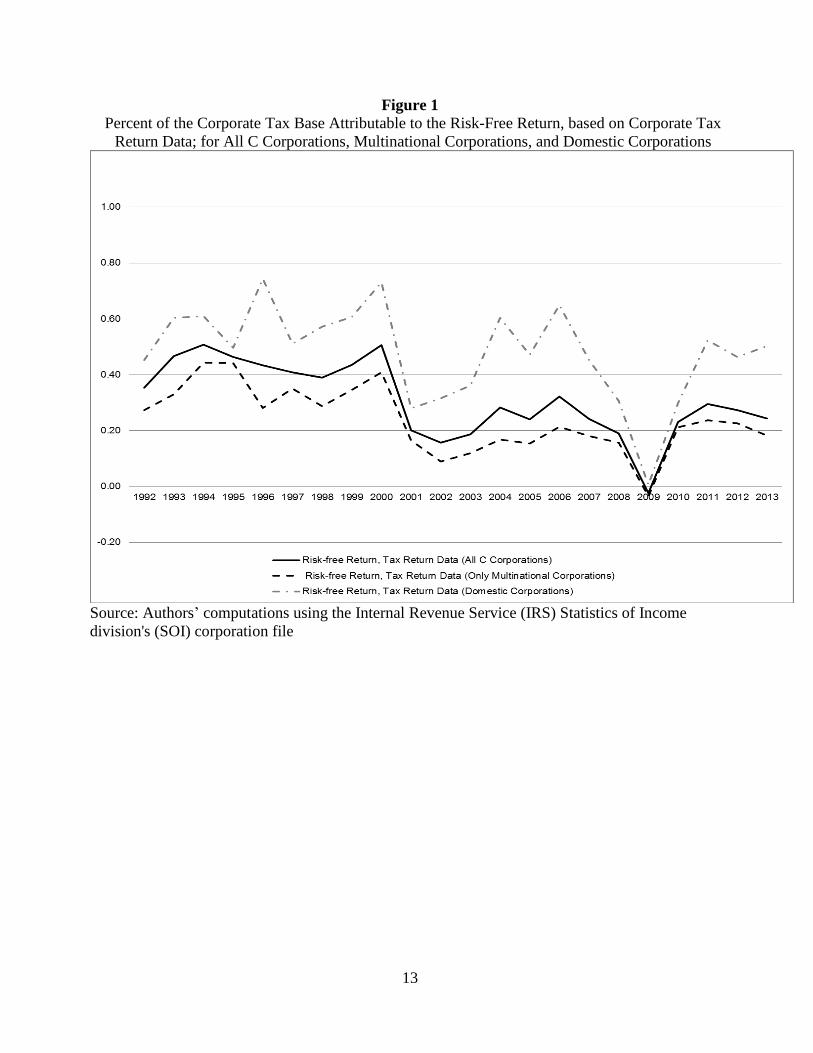
Over time, the pattern of the risk-free return of all C corporations and MNCs is similar,

which is not totally unexpected, since MNC’s comprise a large fraction of total corporate income.

Domestic corporations have a higher and somewhat more volatile risk-free return pattern over time.

All three groups exhibit some cyclical fluctuation, which results in part from the countercyclical

nature of COGS inventory accounting vis a vis inventory expensing. This fluctuation is particularly

7 The estimate is conservative because some taxpayers use a half year convention when taking the first year deduction,

which would imply that the appropriate gross up would actually be 30. Because Section 197 intangibles constitute a

small fraction of capital assets, the impact of this portion of the estimate on the risk-free return to capital is small. 8 Note that MNCs are defined as corporations which a.) file Form 5471 (indicating foreign subsidiary ownership) or b.)

have foreign dividends (from an 80 percent or 100 percent owned foreign corporation) greater than a million dollars.

Domestic corporations are all remaining C corporations that are not MNCs. This is only one of various possible

definitions of multinational versus domestic corporations. 9 Note that MNCs, by definition, have affiliates overseas, which provide them with a variety of opportunities to shift

U.S. profits out of the U.S. tax base. This is particularly problematic with intangible returns because the true return to

intangible assets can be difficult to determine. This valuation difficulty allows intangibles to be mispriced in order to

shift income out of the United States and avoid the statutory U.S. rate. Our estimates do not take such shifted U.S.

income into account. If the shifted profits were actually reported as part of the U.S. tax base, the fraction of the tax base

attributable to the risk-free return would have been even smaller. We perform rough estimates of the change to the risk-

free return that occurs if this shifted income is included in the tax base. We assume that a small fraction of the overseas

income of U.S. MNCs actually is generated in the United States. The fraction is based on the Heckemeyer and

Oversech (2012) elasticity (.8) and an average difference between U.S. and overseas tax rates. The income assumed to

belong to the US tax base is then added to the taxable income denominator to generate a new risk-free return fraction

that accounts for this shifted income. Based on this very rough estimate, the risk-free return fraction is lower over this

period by roughly 5 to 10 percent.

7

evident in 2009, when the ratio became negative due to the large negative affect of inventory

expensing.10

For all three groups, the risk-free return fraction is higher in the first half of the

analysis than in the second half. The tax base of all C corporations averages close to 40 percent

risk-free in the first half and around 25 percent in the second half. MNCs have a somewhat lower

fraction of their tax base attributable to risk-free returns, and exhibit a slightly more dramatic

declining pattern (around 30 percent in the first half and 15 percent in the second half). Domestic

corporations have the highest risk-free return fraction, averaging about 55 percent in the first half

and 40 percent in the second half.

Therefore, for all C corporations, for MNCs, and even for domestic corporations, a

significant portion of the tax base is attributable to excess returns, and the fraction attributable to

excess returns increases over time. This suggests that the difference between an income tax base

and a consumption tax base has declined, and that much of the current tax base would continue to

be taxed under a consumption tax. This trend is somewhat more evident for MNCs. Although we

cannot conclusively establish why excess returns have become more prominent, we can hypothesize

that intangible assets might play an increasingly important role in generating corporate profits.

Intangible assets such as patents and brand names can provide temporary monopoly power that

creates excess returns. If these types of assets are becoming an increasingly important source of

overall profitability, then the fraction of the tax base attributable to the risk-free return could decline

over time. Certain industries are known for having significant intangibles, so the industry analysis

could shed some light on this issue.

10

In particular, the depletion of inventories during the recession implies that expensing of inventory investment is

smaller than the COGS deduction, causing a negative numerator for the normal return fraction. This issue is examined

further in the PDV analysis below and in Appendix A.

8

V. INDUSTRY ANALYSIS

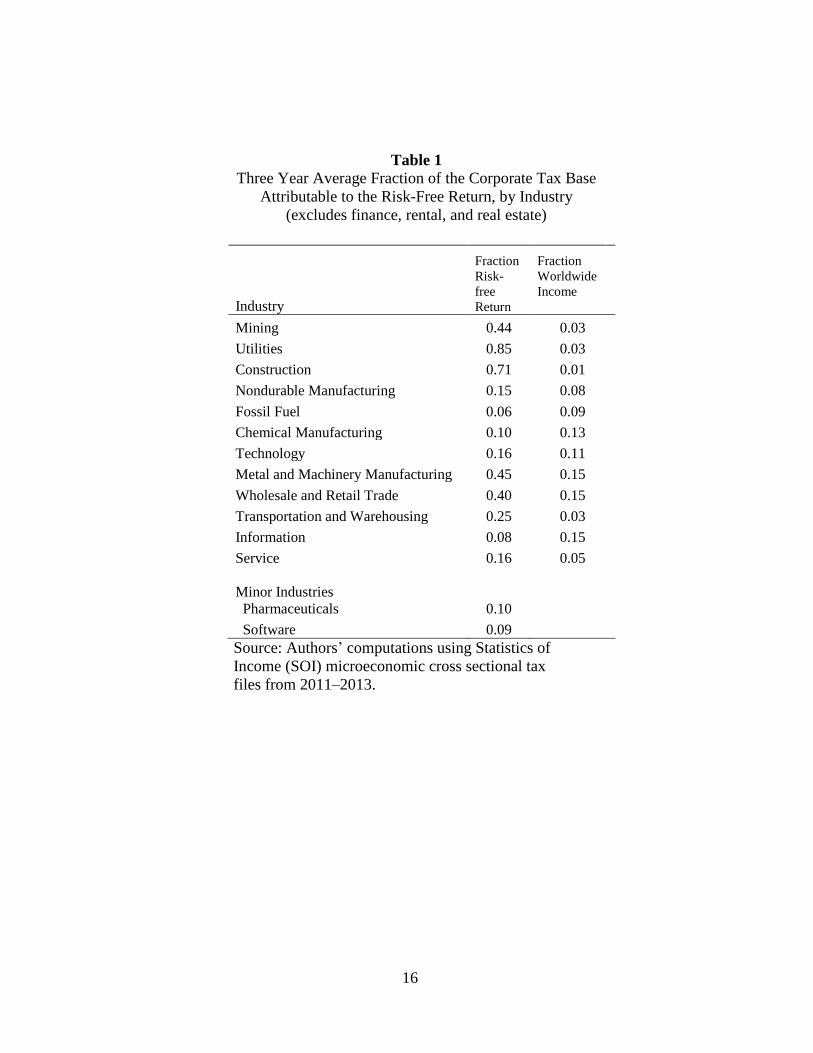
In order to get a sense of how the fraction of the tax base attributable to the risk-free return

varies by industry, we calculate three-year averages (2011-2013) of the risk-free return. To provide

quantitative context, we also report the 2013 fraction of Schedule M-3 reported worldwide book

income by industry. These figures are reported in Table 1.

The risk-free fraction varies substantially by industry. Utilities, construction, and mining all

have very high risk-free return fractions (60+/- percent). Several industries such as transportation,

wholesale and retail trade, and metal manufacturing have risk-free fractions which are about

average (roughly 30 percent to 40 percent). But a few industries, including information,

technology/software, nondurable manufacturing, and chemical manufacturing (including

pharmaceuticals) all exhibit very low risk-free fractions (roughly 10 percent to 20 percent).

Interestingly, most of these industries are also known to hold significant intangible assets. The

calculations therefore suggest that industries that hold intangible assets seem to earn higher than

average excess returns. The fossil fuel industry also has an unusually low risk-free return fraction.

While this industry is not known for holding intangibles, it arguably holds some degree of

monopoly power.

The financial sector is an unusual case, so we exclude it from the aggregate and industry

analysis. Net interest income and other financial items, which are removed in the computation of

the R base, heavily influence the taxable income base of the financial sector. Unlike other

industries, interest income is arguably active income for the finance industry. Therefore, an

alternative definition of the risk-free return potentially needs to be devised for this industry.

Although beyond the scope of this paper, this definition could perhaps be modelled somewhat after

9

the Gentry and Hubbard (1997) definition, by comparing the financial industry’s rate of return with

the risk-free rate of return.

The real estate and rental industries are also excluded from the industry analysis. These

industries hold large amounts of physical structures, so the expensing of tangible capital produces

huge changes in the tax base. This change leads to difficult to interpret risk-free return ratios greater

than one. While again beyond the scope of this paper, further examination of this industry, and a

possible alternative definition of the risk-free return for rental and real estate, is warranted. These

new definitions would be especially useful for an analysis of partnerships, since finance and real

estate are both very important industries in the partnership sector.

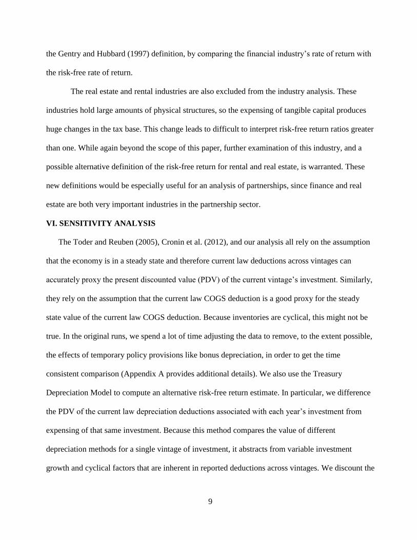
VI. SENSITIVITY ANALYSIS

The Toder and Reuben (2005), Cronin et al. (2012), and our analysis all rely on the assumption

that the economy is in a steady state and therefore current law deductions across vintages can

accurately proxy the present discounted value (PDV) of the current vintage’s investment. Similarly,

they rely on the assumption that the current law COGS deduction is a good proxy for the steady

state value of the current law COGS deduction. Because inventories are cyclical, this might not be

true. In the original runs, we spend a lot of time adjusting the data to remove, to the extent possible,

the effects of temporary policy provisions like bonus depreciation, in order to get the time

consistent comparison (Appendix A provides additional details). We also use the Treasury

Depreciation Model to compute an alternative risk-free return estimate. In particular, we difference

the PDV of the current law depreciation deductions associated with each year’s investment from

expensing of that same investment. Because this method compares the value of different

depreciation methods for a single vintage of investment, it abstracts from variable investment

growth and cyclical factors that are inherent in reported deductions across vintages. We discount the

10

figures using the nominal 10-year Treasury bond rate, which is often equated with a pure risk-free

rate. We compute an alternative estimate of the change in COGS by building a simple model to

compute the PDV of the current law COGS deduction. We then subtract this PDV from each year’s

COGS investment (Appendix A provides additional detail). We again use the nominal Treasury 10-

year bond rate to proxy a risk-free discount rate. We add these PDV estimates to the amortization

estimate and compare the total to the R base to get a PDV estimate of the fraction of the tax base

attributable to the risk-free return.11

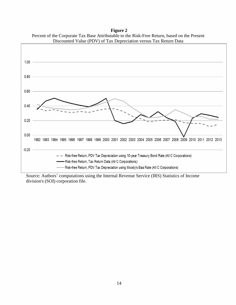
The results of this PDV exercise for C corporations are in

Figure 2.

The PDV comparison smooths some of the volatility over the business cycle, so the estimates of

the risk-free return fraction are smaller than they are using the Toder and Rueben (2005)

methodology. Overall, though, the results are similar to the original estimates. The fraction of the

tax base attributable to the risk-free return declines slowly over time, with the average for the first

half of the period around 35 percent and the average for the second half around 20 percent (both

slightly lower). The difference in pattern over the business cycle between the PDV estimates and

the Toder and Rueben (2005) estimates results from the cyclicality of the reported COGS

deduction. The PDV calculations lessen the impact of cyclicality and hence result in a slightly

different pattern.12

11

For uniformity, we should also have computed the PDV of amortization of Section 197 intangibles, but because of

data limitations and the small magnitude of the investment, we left this field as computed in the Toder and Reuben

(2005) methodology. 12

During economic downturns, the COGS deduction across vintages is often more generous than expensing of COGS

investment, seemingly because inventories are sold down. This results in a negative adjustment in the risk-free return

fraction, and hence reduces the fraction during downturns. The PDV calculations compare COGS depreciation versus

expensing of COGS investment for each vintage of investment. The COGS deduction for a single vintage can never

exceed 100 percent of COGS investment, hence when considering a single vintage, the deduction always represents

slower (or equal) cost recovery relative to expensing. A more sophisticated PDV model than ours might assume time

variant differences in the inventory sales pattern. This would smooth the PDV pattern further. Appendix A provides

additional details.

11

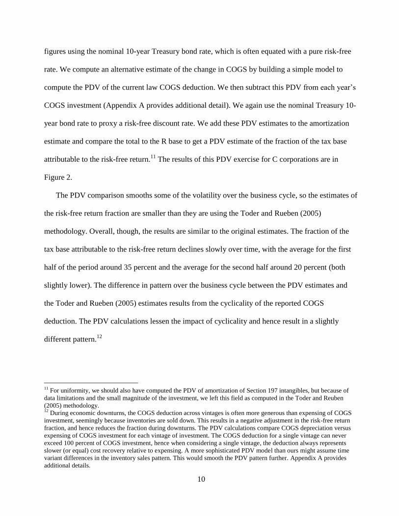
Taxpayers are not completely certain that they will recover all depreciation deductions; for

example, a taxpayer could go bankrupt and not be able to use the deductions. Therefore, as an

alternative to the Treasury 10-year bond rate, we discount deductions using a slightly higher rate

that reflects the possibility that deductions will never be used.13

The higher rate chosen was the

nominal Moody’s Baa corporate bond yield.14

These estimates are also presented in Figure 2, and,

as expected, the estimates are higher using the corporate bond rate as the discount rate, but

otherwise look quite similar.

Both nominal and real interest rates fall substantially over this period, and this decrease

contributes to the decline in the PDV estimate over time. To the extent the interest rate decrease is

due to falling inflation, some of the decline in the measured risk-free return is associated with the

decline in inflation. The decrease in real interest rates, potentially resulting from factors such as

weak global demand and excess savings, suggests that the return to waiting has declined over time.

Overall, falling interest rates potentially explain about half of the decrease in our PDV estimate of

the risk-free return.15

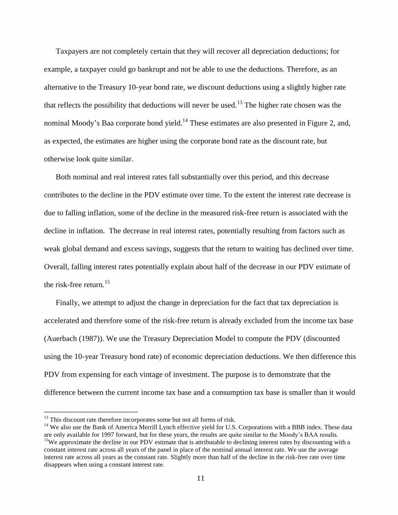
Finally, we attempt to adjust the change in depreciation for the fact that tax depreciation is

accelerated and therefore some of the risk-free return is already excluded from the income tax base

(Auerbach (1987)). We use the Treasury Depreciation Model to compute the PDV (discounted

using the 10-year Treasury bond rate) of economic depreciation deductions. We then difference this

PDV from expensing for each vintage of investment. The purpose is to demonstrate that the

difference between the current income tax base and a consumption tax base is smaller than it would

13

This discount rate therefore incorporates some but not all forms of risk. 14

We also use the Bank of America Merrill Lynch effective yield for U.S. Corporations with a BBB index. These data

are only available for 1997 forward, but for these years, the results are quite similar to the Moody’s BAA results. 15

We approximate the decline in our PDV estimate that is attributable to declining interest rates by discounting with a

constant interest rate across all years of the panel in place of the nominal annual interest rate. We use the average

interest rate across all years as the constant rate. Slightly more than half of the decline in the risk-free rate over time

disappears when using a constant interest rate.

12

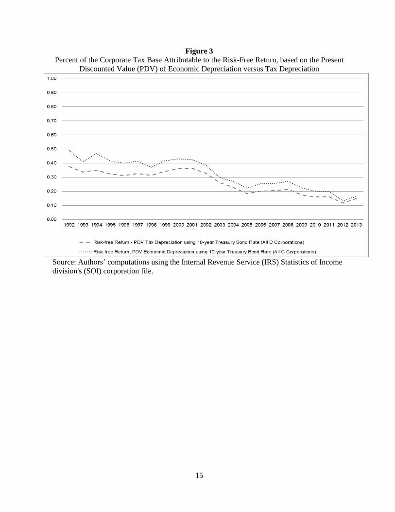
be if the current tax base incorporated economic depreciation rather than accelerated depreciation.

The results of this exercise are presented in Figure 3.

As expected, the estimated risk-free return is somewhat larger based on economic depreciation

than it is based on tax depreciation. This demonstrates that the current income tax system, with its

accelerated tax depreciation, is really a hybrid between a pure income tax and a pure consumption

tax. Overall, the risk-free return fraction based on economic depreciation averages 40 percent

during the first half of the analysis and around 25 percent in the second half.16

Therefore, the

estimated risk-free return based on economic depreciation is roughly 5 percentage points, or 20

percent, higher than estimated risk-free return based on tax depreciation, but it still exhibits a

similar downward trend over time.

VII. CONCLUSION:

In this analysis, we study the time series pattern of the fraction of the C corporation tax base

attributable to the risk-free return. Our computations suggest that the fraction declined over time for

all C corporations, for multinational corporations, and for domestic corporations. This suggests that

the difference between an income tax base and a cash flow tax base has decreased, and it also

suggests that excess returns have become relatively more important to the tax base. The weak

global demand and excess savings associated with declining interest rates potentially contribute to

the decline in the estimated risk-free return over time, and therefore to the increased relative

importance of excess returns. The industry calculations demonstrate that the fraction of the tax base

attributable to excess returns is higher in industries known to hold large amounts of intangible

assets. This suggests that excess returns attributable to intangible assets could also explain some of

the increased importance of excess returns.

16

Coincidentally, these percentages are the same as those estimated using the tax return data; however, the tax return

data is obviously based on tax depreciation rather than economic depreciation.

13

Figure 1

Percent of the Corporate Tax Base Attributable to the Risk-Free Return, based on Corporate Tax

Return Data; for All C Corporations, Multinational Corporations, and Domestic Corporations

Source: Authors’ computations using the Internal Revenue Service (IRS) Statistics of Income

division's (SOI) corporation file

14

Figure 2

Percent of the Corporate Tax Base Attributable to the Risk-Free Return, based on the Present

Discounted Value (PDV) of Tax Depreciation versus Tax Return Data

Source: Authors’ computations using the Internal Revenue Service (IRS) Statistics of Income

division's (SOI) corporation file.

15

Figure 3

Percent of the Corporate Tax Base Attributable to the Risk-Free Return, based on the Present

Discounted Value (PDV) of Economic Depreciation versus Tax Depreciation

Source: Authors’ computations using the Internal Revenue Service (IRS) Statistics of Income

division's (SOI) corporation file.

16

Table 1

Three Year Average Fraction of the Corporate Tax Base

Attributable to the Risk-Free Return, by Industry

(excludes finance, rental, and real estate)

Industry

Fraction

Risk-

free

Return

Fraction

Worldwide

Income

Mining 0.44 0.03

Utilities 0.85 0.03

Construction 0.71 0.01

Nondurable Manufacturing 0.15 0.08

Fossil Fuel 0.06 0.09

Chemical Manufacturing 0.10 0.13

Technology 0.16 0.11

Metal and Machinery Manufacturing 0.45 0.15

Wholesale and Retail Trade 0.40 0.15

Transportation and Warehousing 0.25 0.03

Information 0.08 0.15

Service 0.16 0.05

Minor Industries

Pharmaceuticals 0.10

Software 0.09

Source: Authors’ computations using Statistics of

Income (SOI) microeconomic cross sectional tax

files from 2011–2013.

17

ACKNOWLEDGEMENTS

We are grateful to William Gentry, L. Adam Looney, John Mcclelland, James Mackie III, and

Michael Cooper for helpful comments, suggestions, and assistance, as well as to the discussants and

participants at the National Tax Association’s Spring Syposium. The views in this paper do not

necessarily reflect those of the U.S. Department of the Treasury.

DISCLOSURES

The authors have no financial arrangements that might give rise to conflicts of interest with respect

to the research reported in this paper.

REFERENCES

Auerbach, Alan J., 1993. “Public Finance in Theory and Practice.” National Tax Journal 66 (4),

519–526.

Auerbach, Alan J., and James Poterba, 1987. “Why Have Corporate Tax Revenues Declined.”

NBER Working Paper No. 2118, National Bureau of Economic Research, Cambridge MA.

Cronin, Julie-Anne, Lin, Emily Y., Power, Laura, and Michael Cooper, 2012. “Distributing the

Corporate Income Tax: Revised U.S. Treasury Methodology.” OTA Technical Paper No. 5, U.S.

Department of the Treasury, Office of Tax Analysis, Washington, DC.

Daniel, P., Keen, M., and Charles McPherson (eds), 2010. The Taxation of Petroleum and

Minerals: Principles, Problems and Practice. Routledge, Oxon, United Kingdom.

Gentry, William M. and R. Glene Hubbard, 1997. “Distributional Implications of Introducing a

Broad-Based Consumption Tax” In James M. Poterba (ed.) Tax Policy and the Economy: Volume

11. MIT Press, Cambridge, MA

Gordin, Roger H. and Joel Slemrod, 1988. “Do We Collect Any Revenue from Taxing Capital

Income?” In Lawrence H. Summers (ed.) Tax Policy and the Economy: Volume 2, 89–130. MIT

Press, Cambridge, MA.

Griffith, R., Hines, J. & P. B Sorenson, 2010. “International Capital Taxation,” In Adam, S., T.

Besley & R Blundell (eds.) Dimensions of Tax Design: The Mirrlees Review, 914–996. Oxford

University Press, Oxford, United Kingdom.

Grubert, Harry, 2003. “Intangible Income, Intercompany Transactions, Income Shifting, and the

Choice of Location.” National Tax Journal 56 (2), 221–242.

Heckemeyer, J. and Michael Overesch, 2012. “Multinationals’ Profit Response to Tax Differentials:

Effect Size and Shifting Channels.” Centre for European Economic Research ZEW Discussion

Paper No. 13–045, Mannheim, Germany.

18

Hulten, C. and Frank C. Wykoff, 1981. “The Measurement of Economic Depreciation.” In Charles

R. Hulten (eds) Inflation & the Taxation of Income from Capital, 81–125. Urban Institute Press,

Washington, DC.

Mirrlees, J., Adam, S., Besley, T., Blundell, R., Bond, B., Chote, R., Gammie, M., Johnson, P.,

Myles, G., and James Poterna, 2012. “The Mirrlees Review: A Proposal for Systematic Tax

Reform.” National Tax Journal 65 (3), 655–684.

Organisation for Economic Co-operation and Development (OECD), 2007. “Fundamental Reform

of Corporate Income Tax.” OECD Tax Policy Studies, No. 16, OECD Publishing, Paris, France.

Toder, Eric and Kim Rueben, 2005. “Should We Eliminate Taxation of Capital income?” Paper

prepared for “Conference on Taxation of Capital Income,” September 2005, sponsored by The

Urban Institute, Washington, DC.

19

APPENDIX A

This appendix provides details of the methodologies we use in this paper to compute risk-

free and excess returns. As described above, we use the Statistics of Income (SOI) micro-data tax

files from 1992-2013. We first limit the data to nonfinancial C corporations, although ultimately we

hope to devise a methodology that would allow us to compute the risk-free return for financial

corporations as well. Following Cronin et al. (2012), we convert the tax base into a real income

base (R base) by eliminating capital gains, dividends, and net interest (i.e., subtracting interest

income from the tax base and adding interest deductions back into the tax base).

Our estimates of the change in the tax base attributable to the risk-free return are comprised

of three elements. The first element is the change in the tax base that would result from replacing

the current law cost of goods sold (COGS) deduction with expensing of inventory costs. We

compute this change by summing the cost of labor, purchases, Section 263a costs (which are

uniform capitalization costs), and other costs from Schedule A of the corporate tax return, and

subtracting this sum from reported COGS.

For the second element, we replace the current law (modified accelerated cost recovery

system (MACRS)) depreciation deductions with expensing of tangible investment. During this

time, Congress periodically enacted an important temporary bonus depreciation provision. This

bonus depreciation allowed either 30 percent, 50 percent, or 100 percent (depending on the year) of

tangible capital expensing for equipment. This change significantly affects the value of the

depreciation deductions reported in affected years. Therefore, to get a time consistent comparison,

we recalculate the reported current law depreciation deductions so that bonus depreciation does not

apply. We calculate these figures by substituting the value of MACRS depreciation on bonus

investment for the reported bonus depreciation deduction in the current law depreciation

20

deductions. Therefore, we take the value of equipment investment expensed under bonus, compute

the stream of depreciation deductions associated with that investment, and then add those

deductions back into the year in which they would have been taken in the absence of bonus

depreciation.17

This calculation reduces current law depreciation deductions in years in which the

temporary bonus depreciation provisions are in effect. However, it increases current law

depreciation deductions in years following the expiration of the provision, because deductions

associated with expensed investment are added to the year in which they would have taken place in

the absence of bonus depreciation. The difference between this adjusted current law depreciation

and 100 percent expensing of tangible capital then comprises the second element of the fraction of

the tax base attributable to a risk-free return.

This bonus adjustment differs from the bonus adjustment Cronin et al. (2012) use. They

approximate the value of such deductions with a single estimated aggregate gross up factor. The

methodology we use is more accurate, because it actually computes what depreciation would have

been taken in the absence of bonus depreciation and adds it back to the appropriate year. For this

reason, the total depreciation deductions estimates using the current methodology are somewhat

lower than the ones in Cronin et al. (2012).18

17

Mechanically we add the depreciation deductions in by adjusting each year’s prior year deductions by an appropriate

amount. 18

There are two additional differences between this methodology and the Cronin et al. (2012) methodology. First, they

add software expensing to total expensing. They approximate it by estimating the fraction of the depreciation

deductions reported in the catchall category “Accelerated Cost Recovery System (ACRS) and other depreciation” which

are attributable to software deductions, and then approximate software investment from software deductions. In order to

estimate the fraction of ACRS depreciation attributable to software, they had to estimate how much of it (pre-1986

depreciation) might remain. Attempting to do this estimate in a time consistent time series way is beyond the scope of

this analysis; hence, we do not include expensing of software in our expensing estimate. This exclusion results in a

somewhat lower expensing estimate than Cronin et al. (2012). However, any software investment included in Section

179 (which provides for small business expensing) will be included in our expensing estimates and our PDV estimates

fully account for software in all years because they include all types of investment. The PDV estimates also account for

depreciation versus expensing of Section 179 investment, though we also test undoing Section 179 expensing in a

manner similar to bonus depreciation. The results are nearly identical. However, these differences, as well as the use of

the micro-data files versus the micro-simulation model Cronin et al (2012) use, cause our estimated risk-free return

fractions in 2004 and 2007 to differ somewhat from those reported in Cronin et al (2012).

21

The third element is the change in the tax base that would result from replacing amortization

of Section 197 intangibles (which are acquired intangibles that include goodwill, workforce in

place, patents, copyrights, licenses, permits, franchises, trademarks, customer-based intangibles,

and supplier-based intangibles) with expensing of these intangibles. Section 197 intangibles are

only a small subset of all intangibles. Most self-created intangibles, however, are already expensed

in the computation of taxable income and therefore they are not part of the tax base. We create a

proxy for the amortization of Section 197 intangibles to expensing by first estimating the value of

current year investment in Section 197 intangibles. We do this calculation by grossing up the

amortization deduction for each year’s investment by 15 (since Section 197 intangibles are

amortized over 15 years). We then take the difference between current year amortization and the

current year expensing of this proxy amount.

Finally, we add all three of these components together and compare them to the R based real

taxable income (computed as described in Cronin et al. (2012)). This ratio represents the fraction of

the tax base that is attributable to the risk-free return to capital in each year.

As mentioned above, the accuracy of the Toder and Reuben (2005) methodology relies on

file values of COGS depreciation and tangible capital depreciation being good proxies of steady

state values. Therefore, we try an alternative methodology to test the robustness of their results. In

particular, we substitute the present discounted value (PDV) of the depreciation deduction

associated with each year’s tangible capital investment and the PDV of the COGS depreciation

deduction associated with each year’s COGS investment. For the tangible capital estimates, we use

the Treasury Depreciation Model, which has detailed BEA investment data by industry, asset, tax

depreciation class, and vintage, from 1900 to present. Using this model, we compute the PDV of tax

depreciation deductions for each year’s investment (not including investment in the financial

22

industry). We verify that total nonfinancial investment from the Treasury Depreciation Model is

consistent with total nonfinancial investment from the tax return data. We also try two alternative

discount rates. We first use the nominal 10-year Treasury bond rate in each year (as a proxy for a

risk-free return) and we then use the nominal Baa Moody’s corporate bond rating (to account for

some types of risk). We subtract the PDV from each year’s investment to obtain an estimate of the

change in the tax base from moving to expensing.

For the COGS estimates, we also create a proxy for the PDV of COGS inventory

accounting.19

Based on a comparison of the rate of sales to current year inventories, we estimate

that on average about 90 percent of goods are sold in the year in which they are created. We assume

the rest are sold the following year. We then estimate the PDV of each year’s COGS investment

over two years using the same discount rates as for discounting of tangible capital. In actuality,

however, it appears that the fraction of inventories sold in a given year varies over time. This

suggests that our 90 percent-10 percent split perhaps ought to change depending on whether the

economy is growing or shrinking. If we assume a higher fraction of inventories are sold during

recession years (e.g.; 95 percent-5 percent), this reduces the fraction of the tax base attributable to

the risk-free return in these years and further smooths the PDV estimates. However, we do not have

accurate information on how the sales of a fraction of a given vintage’s inventory changed over

time. For this reason, we use the 90 percent-10 percent fraction and hold it constant over time in our

baseline. We do test the sensitivity of the results to different assumed fractions and the results

generally look similar, with less fluctuation around recessions.

Because MACRS depreciation is actually accelerated relative to economic depreciation, part

of the risk-free return to capital is already excluded from the tax base. We test to see how the

19

In order to better proxy a steady state, this methodology focuses on the current versus proposed law treatment of

current year cost of goods purchases and ignores the treatment of existing inventory as a transition issue.

23

estimate of the risk-free return would differ if the tax system was based on economic depreciation

rather than accelerated depreciation. To do this test, we again use the Treasury Depreciation Model.

We compute, for each year’s investment, the PDV of the stream of economic depreciation

deductions, alternatively using both of the discount rates described above. The Treasury model uses

Hulten and Wykoff (1981) economic depreciation rates and uses historical inflation rates for the

computation of economic depreciation. We then add the PDV of economic depreciation deductions

to the PDV of the COGS deduction to the difference between expensing and amortization of

Section 197 intangibles in order to derive the numerator of the fraction. Next, we adjust reported R

based taxable income to reflect the increase that would result from (lower) economic depreciation

deductions (relative to MACRS tax depreciation deductions). The ratio of the two estimates tells

what the risk-free return fraction would be if the tax system used economic depreciation instead of

tax depreciation.