returns, risk, and financial due diligence* - rmcs incrmcsinc.com/articles/riskreturn.pdf ·...
TRANSCRIPT
CHAPTERS
Returns Risk and Financial Due Diligence CHRISTOPHER L CULP Senior Advisor at Compass Lexecon and Adjunct Professor of Finance Booth School of Business The University of Chicago
JBHEATON Partner Bartlit Beck Herman Palenchar amp Scott LLP and Lecturer The University of Chicago Law School
Returns are the prospective financial rewards from investment Risk is the potential for fluctuations in returns to engender losses If investors are risk averse-as most appear to be-then they should demand higher expected
returns from riskier investments In the wake of the credit crisis and the Bernard Madoff scandal investors and
regulators are clamoring for more rigorous financial due diligence by fund managers institutional investors and other market participants Financial due diligence is the process by which investors try to ascertain among other things the potential risks and returns of a contemplated investment
Both qualitative and quantitative methods are used to determine whether a given investment offers a fair riskreturn trade-off (and what that tradeshyoff is) Due diligence analysts use qualitative methods to examine hard-toshyquantify variables-for example portfolio manager reputation internal control quality reporting adequacy and regulatory compliance Investors employ quanshytitative methods to examine matters that more naturally lend themselves to emshypirical analyses-especially the risk and return characteristics of contemplated investments1
Some potential investments can appear undesirable until the due diligence analyst properly measures their risks and returns at which point the investment may seem more attractive Alternatively other potential investments can look
We are grateful to John Cochrane and Dan Fischel for their comments on earlier drafts The usual disclaimer applies however the opinions expressed herein are the authors alone and do not necessarily reflect those of any organization with which the authors are affiliated or their customers and clients
85
86 Finance Theory
appealing until the due diligence analyst appropriately analyzes risks and returns and determines that the investment is unpalatable
Part of the process of identifying investments with fair riskreturn trade-offs includes spotting investments that seem too good to be true As Judge Richard Posner observed in a Ponzi scheme case Only a very foolish very naive very greedy or very Machiavellian investor would jump at a chance to obtain a return on his passive investment of 10 to 20 percent a month (the Machiavellian being the one who plans to get out early pocketing his winnings before the Ponzi scheme collapses) It should be obvious that such returns are not available to passive investors in any known market save from the operation of luck 2 Financial due diligence helps investors avoid becoming one of those very foolish very naive very greedy or very Machiavellian investor[s 1 that Judge Posner and other actors in the courts look for in such situations
In this chapter we first explain basic concepts of risk and return in financial economics with an eye toward the task of financial due diligence We then illustrate the applications of these concepts in financial due diligence using the example of Bernard Madoff Investment Securities
BASIC CONCEPTS OF RISK AND RETURN IN FINANCIAL ECONOMICS The return on an asset over some period of time (returns are always relative to some time period whether an instant day month year etc) is its payoff over that time period relative to its initial value (ie the value of the asset at the beginning of the period) We summarize some of the most popular ways of measuring returns in Appendix A Most generally the net return on a financial asset from time t to t + 1 is
dl + + PI+ - PI (51)
PI
where PI is the price of the asset at time t XI+ is the payoff to investors at time t + 1 dt+l reflects distributions to investors (eg dividends or interest) at time
t+1 PH is the price of the asset or portfolio at the end of the holding period
The risk of an asset is the potential for returns to fluctuate unexpectedly Returns vary for a number of reasons including but not limited to changes in prices and interest rates (market risk) the nonperformance of counterparties or obligors (credit risk) cash flow shortfalls (funding risk) and forced liquidations of losing positions at unreasonable prices or spreads (liquidity risk)
A key premise of modem financial economics is that return and risk are related-in particular investors expect a higher return for bearing higher risk When an asset pays off a known amount with certainty that asset is called risk-free Competition in the market for risk-free assets will force the rate payable on riskless assets to the risk-free rate3
87 RETURNS RISK AND FINANCIAL DUE DILIGENCE
Excess Returns and Alpha
Risk-averse investors will demand a return in excess of the risk-free rate to compensate them for bearing risks they prefer to avoid Risks to which investors are averse are risks that lead to losses-so-called downside risks Some investors are content with low returns as long as they face limited downside risk Others are willing to bear more downside risk in the pursuit of higher returns
In theory only downside risks that investors cannot eliminate by diversificashytion should earn higher expected returns Such risks are called systematic risks Because no investor can eliminate systematic risk simply by adding other assets with systematic risk to a diversified portfolio the asset must offer a return comshymensurate with its systematic risk to persuade the investor to hold the asset
Risks that the investor can eliminate by holding the asset in a diversified portfolio by contrast are called idiosyncratic risks Tn equilibrium investors should not earn a return for bearing idiosyncratic risk which is diversifiable by most investors4 Otherwise all investors would have an incentive to add any asset offering a return for idiosyncratic risk to their already diversified portfolio The idiosyncratic risk would disappear in the portfolio leaving only the return Such free lunches cannot survive in competitive capital markets
Much research in financial economics aims at understanding the risks for which investors demand compensation in capital markets That is financial economists seek to understand the sources of systematic risk and the returns that investors demand for bearing those risks If we could measure systematic risk perfectly we then could estimate the expected return actually being offered by the asset E(r) and compare it to the expected return E(r) that compensates for the assets systematic risk The difference if any between the two is known as alpha
IX = E(r) E(r)
A zero or negative alpha indicates that the investment is just compensating or undercompensating investors for the risks that affect the underlying payout on the security or portfolio But if alpha is positive the investment is overperforming relative to its measured risks That is the reason many investors claim to seek alpha-investments with positive alpha are offering expected returns that more than compensate for their risk
How much return an asset should pay to compensate for its systematic risk depends on the sources of systematic risk the exposure of the asset to those sources and the premiums that investors demand for bearing that risk Answering those questions requires a model of market equilibrium for capital assets often referred to as asset pricing models Different asset pricing models will in general assume the existence of different sources of systematic risk and thus typically give rise to different estimates of E(r)5
The Capital Asset Pricing Model
The capital asset pricing model (CAPM) is the simplest and best-known theoretical asset pricing modeL In the CAPM the only source of systematic risk is the extent to which an assets return moves together (covaries) with the return of the weighted
88 Finance Theory
average of all other assets where the weights are the market values of all of the other assets in the world
The idea is fairly simple Suppose that you could buy a little bit of every asset in the world and that your own personal portfolio had the same rate of return as the weighted average of all assets in the world-that is your own portfolio of risky assets is just a tiny version of the whole portfolio of world wealth Suppose further that you prefer more money to less but that at your current wealth the pain of losing a dollar hurts more than the pleasure of gaining a dollar feels good
Now consider anyone asset in the world If the asset performs well (earns good returns) when all of your other assets are doing well that is doubtless a good thing But the problem is that you are earning money from that asset when you are already earning money on everything else And it works the other way If that asset is moving with the rest of your wealth then it is going to perform poorly when the rest of your assets also are doing poorly Thats not good So the more an assets return covaries with the rest of the wealth in the world the more you are going to want to get paid to hold that asset-that is the higher the expected return you will demand
In the CAPM the systematic risk is the strength of the covariance between the returns on a given asset and the returns to the rest of the wealth in the world That is the CAPM return that investors can expect on some asset or portfolio j E(rj) is related to its systematic risk as follows
(52)
where rj is the return on asset or portfolio j r m is the return on the market portfolio of world-invested wealth rf is the risk-free rate ~j is a measure of the extent to which the returns rj and rm move
together-namely the coefficient in a regression of asset js excess reshyturns on the markets excess returns
or
Cov(rj rm) ~ - ----shy
- Var(rm)
The only source of systematic risk in the CAPM-and the only thing driving differences in expected returns given rm and rris the assets~
To determine whether there is any alpha we take a sample of N historical returns on a portfolio j and run the following regression
(53)
for t = 1 N
89 RETURNS RISK AND FINANCIAL DUE DILIGENCE
If the asset earned returns that compensated for its CAPM risk and the CAPM correctly models asset returns (this is an important assumption) then the estimated intercept u in regression (3) should be zero A positive estimated alpha is evidence that the asset earned more on average than the CAPM predicted
Interpretations of positive estimated alphas can be challenging If the CAPM is true the estimated alpha is good evidence of positive abnormal returns-in other words an investment that beat the market But it is much more difficult to interpret the positive alpha if the CAPM is not a good description of asset pricing In that case the positive alpha may be due entirely to the omission of some other risks for which the investors holding the asset were compensated but which is not reflected in the CAPM The asset will have earned higher average returns than the CAPM predicted not because of any mispricing that reflected the opportunity for returns above those necessary to compensate for risk but instead because those returns compensated for sources of risk omitted from the CAPM
Other Asset Pricing Models
Much empirical evidence suggests that the CAPM does not adequately capture all sources of systematic risk in asset returns The co-movement of returns with other variables helps explain these deviations from the CAPM Asset pricing models that include these variables often characterize expected excess returns as
E(rj) - rf = ~ljOt + fujlgt + + ~kj~ (54)
where ~kj is the kth regression coefficient of asset js excess return on the kth risk factor
Bk is the risk premium of the kth risk factor
The risk factors are proxies for economic variables with which investors are concerned in defining good and bad times In the CAPM the only such risk factor was co-movement with the market
A currently popular version of the general model shown in equation (54) is the Fama and French (1993) three-factor model which describes expected excess returns on an asset or portfolio j in terms of three systematic risk factors
(55)
where 3 is the excess return on the market (the same factor used in the CAPM) 85MB is a variable formed from the difference in returns to big versus small
market capitalization stocks (designed to capture the observed factor of firm size in explaining differences in average returns across stocks)
8HML is a variable formed from the difference in returns on stock with high versus low book -to-market ratios (designed to capture the observed explanatory factor of such measures in explaining differences in average returns across stocks)
90 Finance Theory
The various Ws are the respective regression coefficients A four-factor version of the model also includes a variable designed to capture the tendency of recent good and bad performance to continue known as the momentum effect
Like the CAPM running a regression of the form in equation (55) generates an estimated intercept that should be zero if the Fama-French model is a true representation of the relation between expected excess returns and systematic risk A positive estimated intercept indicates that the average return of the asset or portfolio exceeds the risk-free rate by more than the systematic risk premium Also like the CAPM the positive intercept may reflect abnormal performance unexplained by risk or alternatively misspecification of the asset pricing model that has omitted proxies for the true sources of systematic risk
Measures of Total Risk
To augment or obviate the search for an appropriate asset pricing model to estimate alpha many analysts also employ measures of returns relative to some measure of total risk that does not attempt to decompose return fluctuations into systematic and idiosyncratic components One such measure is the Sharpe ratio6
where SRi is the Sharpe ratio on asset or portfolio j f i is the average return on asset or portfolio j j is the volatility of returns on that asset or portfolio
Volatility is often estimated as the standard deviation of returns over an historical period perhaps using rolling moving averages or more structured models of the evolution of volatility over time
A problem with using the Sharpe ratio for financial due diligence however is its measurement of risk using only the volatility of excess returns Volatility is a symmetric measure of risk that reflects deviations both above and below average returns But if the true return distribution is negatively skewed or fatshytailed volatility is an incomplete description of return dispersion And as noted earlier it is the downside risk with which most investors are more concerned
Consider for example a portfolio that consists of short positions in out-of-theshymoney equity put options The portfolio earns a premium as long as stock prices do not decline significantly But if stock prices collapse the options move into-theshymoney and the value of the portfolio crashes Yet the volatility of the payoff on the short option portfolio is lower than the volatility of a similar portfolio invested in the stocks underlying the puts In both portfolios investors lose when share prices decline But in the stock portfolio investors make money when prices rise unlike the option portfolio in which the maximum payoff is the premium collected The distribution of payoffs on the option portfolio thus is truncated which reduces the estimated volatility of returns That lower volatility however results from chopping off the potential upside of the strategy Volatility thus has been reduced at the expense of negative skewness and fat tails in the payoff distribution As such
91 RETURNS RISK AND FINANCIAL DUE DIUGENCE
it is by no means clear that the option portfolio is less risky than the stock portfolio even though the returns on the former are less volatile than on the latter
To measure the riskreturn ratio for an asset or portfolio with skewed andor fat-tailed returns an analyst may instead evaluate average excess return relative to an estimate of downside risk (DSR) Unlike volatility DSR measures the risk of only those returns below the average or some target The analogue of the Sharpe ratio for measuring average excess returns per unit of DSR is the Sortino ratio
Sortino Ratio = FD~R
Quite a few different ways of measuring DSR can be used to calculate the Sortino ratio One such measure the downside semi-standard deviation (DSSD) is defined as
1 DSSD= L
M
(F -rtFM
1 strltFj
where M is the number of returns in the sample below the average return DSSD thus measures the so-called bad part of the standard deviation If the underlying return distribution has a fat left-hand tail the DSSD provides a better measure of risk than volatility
Another popular measure of DSR is value at risk (VaR) For an estimated disshytribution of potential returns VaR measures the return threshold that the investor expects to exceed (1 - X) percent of the time where X is usually set at 1 pershycent or 5 percent A 99 percent monthly VaR of -15 percent for example means that the portfolio is expected to generate monthly returns below -15 percent only 1 percent of the time The underlying return distribution used to compute VaR can be generated parametrically nonparametrically by simulation analysis or with some mixture of those methods8
A significant drawback of VaR is that it does not tell us the magnitude of potential losses below the critical level A 99 percent monthly VaR of -15 percent suggests that returns should not be below -15 percent more than 1 percent of the time but it does not tell us whether the 1 percent of violations consist of- say -16 percent returns or -1600 percent returns To address this market participants sometimes define VaR in terms of conditional expected loss otherwise known as tail VaR or t-VaR
Analysts typically compare a calculated riskreturn ratio with the risk return profile of similar assets For example Exhibit 51 shows historical return risk and returnrisk ratios for the CRSPValue-Weighted Portfolio ofNYSE NASDAQ and AMEX stocks from 1947 to 2008 All of the measures of return relative to risk are below 050 The definition of risk moreover changes the results noticeably The Sortino ratio using 95th percentile VaR as a measure of DSR for example is appreciably lower than the Sharpe ratio
92 Finance Theory
Exhibit 51 Risk and Return Statistics on the CRSP Value-Weighted Portfolio of NYSE NASDAQ and AMEX Stocks 1947 to 2008
Monthly Annual
Returns Average Marker Return 0924 11981 Average 3D-day T-Bill Return 0377 4659 Average Excess Returnb 0546 7323
Risk Volatility of Excess Returns 4251 18149 DSSD of Excess Returns 4723 20897 95th Percentile VaR of Excess Returns C 6513 22293
ReturnRisk Ratios Sharpe Ratio 01286 04035 Sortino Ratio (DSSD) 01157 03504 Sortino Ratio (VaR) 00839 03285
acRSP Value-Weighted Portfolio (including distributions) bAverage market return minus average 3O-day T-bill return CAbsolute value of fifth percentile excess return Source Center for Research in Security Prices
PUTTING THEORY INTO PRACTICE-THE MADOFF EXAMPLE We now illustrate the application of riskreturn analysis to financial due diligence by examining the detection of a Ponzi scheme In a Ponzi scheme the promoter solicits funds from customers for investment in some portfolio or strategy but little orno investing actually occurs Redemption requests and distributions are financed by cash received from new participants in the scheme-robbing Peter to pay Paul as it were-and the remaining cash is distributed to the participants in the fraud
Because almost aU investment managers who appear to have abnormally high average returns will attribute their results to skill the self-reported performance explanations of investment managers are likely to hold little weight in the due diligence analysis Investment managers do not after all self-proclaim their fraudulent investments
The problem is especially difficult when Ponzi schemes do not promise supershyhigh returns When long-run average returns are just high enough to be enticing but not so high as to be obviously unrealistic then the tools we have discussed thus far can be valuable components of the due diligence process We illustrate using the case of Bernard L Madoff Investment Securities (Madoff in the pages that follow)
Madoffs Ponzi Scheme In the largest investor fraud by an individual in history Madoff primarily marshyketed a single investment strategy-known as a split strike conversion-in which he claimed to be purchasing blue-chip stocks in the SampPIOO Index and simultaneously selling out-of-the-money calls and buying out-of-the-money puts on the SampP 100
93
r RETURNS RISK AND FINANCIAL DUE DILIGENCE
r
Index Normal enough in its own right a split strike conversion strategy is essenshytially just a stock index arbitrage program and as such should have relatively low risk and generate modest returns
Yet Madoff boasted average returns of nearly 105 percent per annum for the 17 years during which the Ponzi scheme went undetected Even when the market fell nearly 40 percent through November 2008 Madoff was still reporting a positive 56 percent year-to-date return (Applebaum et a1 2008)
Ponzi schemes generally fall apart when larger-than-expected redemptions ocshycur But that never happened with Madoff Ifnot for the collapse of equities during the credit crisis Madoffs fraud might have remained undiscovered for many more years Madoffs scheme apparently went undetected for so long part because it was an affinity fraud aimed at the wealthy Jewish community in New York and Palm Beach Within that community Madoff was a well-known figure with impeccable references his investors trusted him Indeed some within Madoffs target affinity group report having tried to invest with him but having been turned away-no doubt adding to his appea19 In addition Madoffs returns were generally not so high as to be completely ridiculous on their face
A RiskReturn Analysis of a Madoff Feeder Fund
Most of Madoffs money came from feeder funds that secured investments from customers and then used Madoff as either the investment manager or broker To analyze the risk and return of Madoffs scam we obtained returns from July 1989 through December 2000 on one of Madoffs largest feeder funds1O Although some of Madoffs feeder funds had other investments we understand that the fund we examined was invested almost exclusively with Madoff
Alpha Exhibit 52 shows Madoffs estimated alpha from the CAPM and the Fama-French model regressions-equations (2) and (5) respectively If we run a CAPM regresshysion of the feeder funds excess returns on the market portfolios excess returns we get a statistically significant estimated a of 07251 percent per month In the naIve CAPM world it looks like Madoff was earning about 75 basis points per month above the return commensurate with the systematic risk of the market The Fama-French regression yields a similar estimate of 07209 percent per month adding the two additional proxies for systematic risk only reduces average returns by about half a basis point per month
Using both the CAPM and Fama-French models it appears as though Madoffs feeder fund was adding significant value in excess of the systematic risk of the fund As noted earlier these positive alpha estimates could be the result of model misspecification But part of the due diligence process is identifying red flags like this one and following up with additional qualitative and quantitative analysis
Returns Relative to Total Risk Measures Exhibit 53 shows monthly returns from July 1989 through December 2000 on the CRSP Value-Weighted Portfolio compared to Madoffs monthly returns The average monthly return on Madoff was 118 percent as compared to an average monthly return on the market of 124 percent over this period As Exhibit 53 also
94 Finance Theory
Exhibit 52 Alpha Regressions of Madoff Feeder Fund Returns
CAPM Fama-French
0007251 0053397
nla nla 138
00727
0007209 0053783
-004799 -001809
138 01147
plt 5 p lt 1
shows however Madoffs returns exhibited very low volatility--)83 percent per month as compared to 408 percent per month for the market
Despite average returns slightly below the market the Sharpe and Sortino ratios for Madoff are well above the market as shown in Exhibit 54 The Sharpe ratio over this period was 09516 for Madoff as compared to 02028 for the market And Madoffs Sortino ratios (measured with DSSD and VaR respectively) were 10730 and 29515 compared to the market Sortino ratios of 01741 and 01465
Moving down the rows in Exhibit 54 average returns are divided by increasshyingly conservative measures of risk As expected the riskreturn ratios for the market decline as the measure of risk in the denominator increases But the
~m~~~m~~~~~~~~~~~~~~~~~~~~~~~m~~888 3~~3~~3~~3~i3~3~~3~~s~is~~3~~3~~3~JZ~Jz~Jz~Jz~Jz~Jz~Jz~Jz~Jz~Jz~Jz~Jz
-CRSP Value-Weighted Portfolio - Madoff Feeder Fund
Exhibit 53 Monthly Returns on the Market versus Madoff Feeder Funds July 1989 through December 2000 Source Center for Research in Security Prices
E I ii II ~ s C 0 il
15
10
5
0
-5
-10
-15
-20
95 RETURNS RISK AND FINANCIAL DUE DILIGENCE
Exhibit 54 Sharpe and Sortino Rations Madoff versus CRSP Value-Weighted Portfolio July 1989 through December 2000
Madoff Market
Sharpe Ratio 09516 02028 Sortino Ratio (DSSD) 10730 01741 Sortino Ratio (VaR) 29515 01465
Madoff portfolio shows the opposite pattern-increasing riskreturn ratios for progressively more conservative measures of risk That indicates extremely thin tails in Madoffs return distribution vis-a-vis the market In other words not only do Madoffs returns exhibit little variation around the average they also include few bad months
Both the levels of the riskreturn ratios and the thin-tailed distributions they indicate represent additional red flags Although fraud is not the only possible exshyplanation for the patterns in Exhibit 54 the data indicate that further due diligence is likely warranted
Persistence and Serial Correlation Another indicator of potentially too-good-to-be-true investments is excessive pershysistence in returns Efficient capital markets are generally thought to follow close to random walks especially over holding periods of a month or longer As such significant persistence in returns is a red flag to ask additional questions about why the performance of an asset or portfolio is seemingly so stable over time
Return persistence is measured statistically by looking at serial correlation (aka autocorrelation) Specifically we can run the following regression
q
rt+ = Po +L Pkrt-k + lOt+
k=l
where q is the number of lagged returns that we want to examine The regression coefficient Pk is the partial autocorrelation of returns at the kth lag If returns fluctuate randomly Pk should be zero at all lags Positive estimated autocorrelations indicate persistence in returns-that is an unusual high return in one period is likely to be followed by an unusually higher return in the next period
The number of autocorrelation lags that an investor should examine depends on the frequency of available mark-to-market returns and the quality of that data In annual returns statistically significant positive autocorrelations at the one-year lag should be enough to raise an eyebrow With monthly returns looking at two or three lags is probably adequate
Positive autocorrelation also reduces estimated volatility Returns that exhibit persistence thus will tend to be less volatile and to have higher Sharpe ratios than returns following a random walk The greater the persistence of returns the lower is the estimated volatility of returns and the higher the Sharpe ratio So even if positive autocorrelations show up for good reasons further due diligence still may well be indicatedll
96 Finance Theory
The first three partial autocorrelation coefficients on market portfolio returns are all statistically indistinguishable from zero just as we would expect But for Madoff the partial autocorrelations are -019 024 and 019 for the first three lags all of which are statistically significant
The positive autocorrelation on the second and third lags show persistence in returns that might be expected from a Ponzi scheme Although returns persistence can be generated by infrequent marking to market of the underlying securities Madoffs supposed focus on highly liquid SampP 100 stocks and options suggests that those autocorrelations cannot be explained by nonsynchronous trading or illiquidity alone
The estimated autocorrelation at the first lag however is negative That is more traditionally associated with phenomena such as market overreactions or prices that bounce between bids and offers The same thing would also be consistent with a fictional pricing scheme that took average prices and then marked them up one month and down the next But the explanation is not immediately obvious from the data
So once again we have a potential red flag-but only a potential one Although the autocorrelations in the Madoff fund are consistent with a fictional-price Ponzi scheme there are other explanations for these estimates The autocorrelations thus are not conclusive on their own but should be the catalyst for asking additional questions
CONCLUSION In theory identifying opportunities that are seemingly too good to be true can be accomplished by looking for abnormally high alphas The problem of course is that the appearance of uncharacteristically high average excess returns may arise for different reasons (1) the investment manager or trader is engaged in willful deception or fraud (2) the investment manager or trader is pursuing authorized and legitimate investments but the measurement does not provide a true picture of risk and return due to errors in data or methodology (3) the investment manager has been lucky or (4) the investment manager has genuine skill But in practice the seemingly insurmountable empirical difficulties in testing asset pricing models makes it virtually impossible to distinguish between alphas that are actually posshyitive and positive alpha estimates that are positive because of a misspecified asset pricing modeL
In the Madoff example warning signs were present in the data as of late 2000 But even with the benefit of hindsight those warning signs were not unshyambiguously indicative of fraud in and of themselves Nevertheless the warning signs were sufficient to indicate that additional analysis-both quantitative and qualitative-may well have been warranted
APPENDIX A COMMON DEFINITIONS OF RETURN A return is the payoff on a financial asset or portfolio relative to the initial value of that investment Returns generally can be measured in one of three ways discrete holding period returns continuously compounded returns or investment accounting returns
97 RETURNS RISK AND FINANCIAL DUE DILIGENCE
Discrete Holding Period Returns
A holding period return is the return on an investment over some period of time during which the investor is presumed to hold the asset The two most basic measures of holding period returns are gross and net per-period returns
dt+1 + Pt+l
PI
dl+1 + PI+ - PI R TII+1 = = 11+1 1
PI
where PI is the time t price of the asset and dt+1 reflects any distributions to the investor such as dividends or interest payments12
We also often want to know the effective N -period return on an asset assuming the payoff on the asset is reinvested at the end of each holding period successively for N periods An investment of $1 at time t that is rolled over for N periods yields a time t + N value of
N
VI+N = n(1 + Tl+j-lt+j)
j=1
The effective return over N periods is then calculated as
1
Ttt+N = V~N - 1
1
TU+N = [(1 + TU+1)(1 + TII+1) (1 + TI+N-lI+N)]N -1
1 rU+N = [RII+1RI+11+2 (RI+N-1t+NrN 1
Careful attention must be paid to the presumed compounding frequency in multiperiod return calculations In general an asset whose return is compounded q times per year over N years has an N-year effective holding period return of
where
VI fi (1 + rl+j-1t+j )
j=l q
Continuously Compounded Returns A continuously compounded return is the instantaneous return on an investshyment assuming that all distributions are continuously reinvested In general the
98 Finance Theory
continuously compounded return (aka geometric return) can be calculated from the corresponding holding period return r as follows
r CC = In(l + r)
In practice continuously compounded returns are often computed as the log difference in prices between two periods An N-period geometric return for exshyample is
Investment Accounting Returns
Investment managers must calculate returns to conform to regulations or guidelines promulgated by supervisors and accounting organizations Such investment accounting measures of return are often more difficult to calculate than holding period returns because they must take into account any contributions or withdrawals
The ideal investment accounting measure is a true time-weighted returnshyessentially a holding period return in which individual holding periods are defined as trading days At the end of any day t the value of the portfolio is defined as
ve = PI + dt
where PI is the mark-ta-market value of the portfolio at the end of day t and dt
reflects any income or distributions on day t The value of the portfolio at the beginning of day t is
where Ct reflects any cash withdrawals or contributions at the end of prior holding period t - 1 The time-weighted gross return over day t then is just
_ veRTWR
t - litb
and the N-period net holding period return is
rr~~ (0 Ri+7R) - 1
The principal reason that a true time-weighted return requires daily holding periods is that cash contributions and withdrawals may occur at any time A manager thus needs to know values and returns on each day in order to account for cash distributions properly
99 RETURNS RISK AND FINANCIAL DUE DILIGENCE
r Many portfolio managers however do not have access to dail y mark-to-market
prices or are concerned about the quality of daily prices on illiquid positions As an alternative investors often compute approximate time-weighted returns (often misleadingly referred to as dollar-weighted returns) using the Modified Dietz method in which the N-period return is approximated as
rMDielz II+N
where Cj is any cash withdrawal or contribution on date j and
TIt+N - Ttt+i TI+j = (56)
Ttt+N
where Ttt+j is the total number of days in the holding period from t to t + j Finally some investment managers compute a naIve dollar-weighted return
on a portfolio as follows
DWR Vi+N rtt+N = --V-I-shy
where K
Vi+N L Ck(l + vkrk
k=l
where K is the total number of days on which a contribution or withdrawal occurred in the holding period from t to t + N
k is an index variable indicating each of those withdrawal dates Tk is as defined in equation (56) lJ k is the internal rate of return on the portfolio at k
NOTES 1 Not all market participants and due diligence analysts are created equaL Most of our
comments here are intended to apply to relatively sophisticated institutional investors
2 Scholes v Lehman 56 F3d 750 760 (7th Cir 1995)
3 The risk-free rate will differ depending on the timing of the certain payoff of course The risk-free rate for an investment that pays off in a year will in general be different from the risk-free rate for an investment that pays off in two years and so on
4 There are some exceptions most of which owe to capital market frictions For a discusshysion see Cochrane and Culp (2003)
5 For a review of the main asset pricing models see Cochrane (2005)
6 See Sharpe (1966 and 1994)
7 Because we are really interested in knowing what the risk of an asset or portfolio will be and not what it was measures of risk in the Sharpe ratio can be even more useful
100 Finance Theory
when based on estimates of expected future volatility reflected in market prices Optionshyimplied volatility for example is a forward-looking estimate of volatility
8 One popular method of measuring VaR known as the parametric normal method uses volatility to compute VaR As a scaled measure of standard deviation this does not add much to risk estimates that on volatility directly But this is just one possible way to measure VaR In general VaR can also be measured in ways that do not rely exclusively on volatility and that allow for skewed and fat-tailed return distributions See for example Culp (2001)
9 See Biggs (2009)
10 Subsequent references to Madoffs performance refer to this single feeder fund We are grateful to Andy Lo for prOViding us with the feeder fund return data
11 Various methods are available to adjust Sharpe ratios and other performance measures for autocorrelation that arises when hedge funds and private equity funds engage in return smoothing (for either legitimate or questionable purposes) For a good discussion see Getmansky Lo and Makarov (2004) and Lo (2001 and 2008)
12 If distributions are paid before the end of the holding period they can easily be restated to time t + 1 values
REFERENCES Applebaum B D S Hilzenrath and A R Paley 2008 All just one big lie Washington Post
(December 13) Biggs B 2009 The affinity Ponzi scheme Newsweek Ganuary 12) Cochrane J H 2005 Asset pricing Rev ed Princeton NJ Princeton University Press Cochrane J H and C 1 Culp 2003 Equilibrium asset pricing and discount factors
Overview and implications for derivatives valuation and risk management In Modern risk management A history ed Peter Field London Risk Books
Culp C 1 2001 The risk management process New York John Wiley amp Sons Fama E E and K R French 1993 Common risk factors in the returns on stocks and bonds
Journal ofFinancial Economics 333-56 Getmansky M A W 10 and I Makarov 2004 An econometric model of serial correlation
and illiquidity in hedge fund returns Journal ofFinancial Economics 74529-609 Lo A W 2001 Risk management for hedge funds Introduction and overview Financial
Analysts Journal 5716-33 2008 Hedge funds An analytic perspective Princeton Nl Princeton University Press
Sharpe W 1966 Mutual fund performance Journal of Business 39119-138 -- 1994 The Sharpe ratio Journal of Portfolio Management 2149-58
ABOUT THE AUTHORS Christopher L Culp is a senior advisor with Compass Lexecon adjunct professor of finance at The University of Chicagos Booth School of Business Honorarprofesshysor at UniversWit Bern in the Institut fUr Finanzmanagement managing director of Risk Management Consulting Services Inc and an adjunct fellow at the Comshypetitive Enterprise Institute He teaches graduate courses on structured finance insurance and derivatives and provides consulting services and testimonial exshypertise in those areas He is the author of four books the co-editor of two books and has published numerous articles He holds a PhD from The University of Chicagos Booth School of Business
101 RETURNS RISK AND FINANCIAL DUE DILIGENCE
J B Heaton is a litigation partner with BartHt Beck Herman Palenchar amp Scott LLP He received his MBA JD and PhD (financial economics) from the University of Chicago in 1999 He regularly lectures and publishes on topics in law and finance Dr Heatons law practice focuses on litigation for hedge funds and private equity funds Dr Heaton teaches as a lecturer at the University of Chicago Law School and previously has taught as an adjunct professor at Northwestern University Law School and as an adjunct professor of finance at Duke University
FINANCE ETHICS
Critical Issues in Theory and Practice
John R Boatright
The Robert W Kolb Series in Finance
~ WILEY
John Wiley amp Sons Inc
Copyright copy 2010 by John Wiley amp Sons Inc All rights reserved
Published by John Wiley amp Sons Inc Hoboken New Jersey Published simultaneously in Canada
No part of this publication may be reproduced stored in a retrieval system or transmitted in any form or by any means electronic mechanical photocopying recording scanning or otherwise except as permitted under Section 107 or 108 of the 1976 United States Copyright Act without either the prior written permission of the Publisher or authorization through payment of the appropriate per-copy fee to the Copyright Clearance Center Inc 222 Rosewood Drive Danvers MA 01923 (978) 750-8400 fax (978) 646-8600 or on the Web at oWWcopyrightcom Requests to the Publisher for permission should be addressed to the Permissions Department John Wiley amp Sons Inc 111 River Street Hoboken NJ 07030 (201) 748-6011 fax (201) 748-6008 or online at http wwwwileycomgopermissions
Limit of LiabilityDisclaimer of Warranty While the publisher and author have used their best efforts in preparing this book they make no representations or warranties with respect to the accuracy or completeness of the contents of this book and specifically disclaim any implied warranties of merchantability or fitness for a particular purpose No warranty may be created or extended by sales representatives or written sales materials The advice and strategies contained herein may not be suitable for your situation You should consult with a professional where appropriate Neither the publisher nor author shall be liable for any loss of profit or any other commercial damages including but not limited to special incidental consequential or other damages
For general information on our other products and services or for technical support please contact our Customer Care Department within the United States at (800) 762-2974 outside the United States at (317) 572-3993 or fax (317) 572-4002
Designations used by companies to distinguish their products are often claimed by trademarks In all instances where the author or publisher is aware of a claim the product names appear in Initial Capital letters Readers however should contact the appropriate companies for more complete information regarding trademarks and registration
Wiley also publishes its books in a variety of electronic formats Some content that appears in print may not be available in electronic formats For more information about Wiley products visit our Web site at wwwwileycom
Library of Congress Cataloging-in-Publication Data
Boatright John Raymond 1941shyFinance ethics critical issues in theory and practice John R Boatright
p cm (The Robert W Kolb series in finance) Includes bibliographical references and index ISBN 978-0-470-49916-0 (hardback) ISBN 978-0470-76809-9 (ebk)
ISBN 978-0470-76810-5 (ebk) ISBN 978-0470-76811-2 (ebk) 1 Business ethics 2 Finance-Moral and ethical aspects 1 Title
HF5387B64 2010 1744-dc22 2010010867
Printed in the United States of America
10 9 8 7 6 5 4 3 2 1
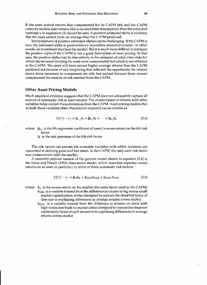
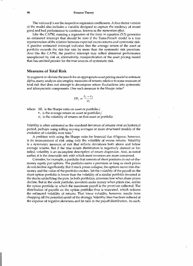
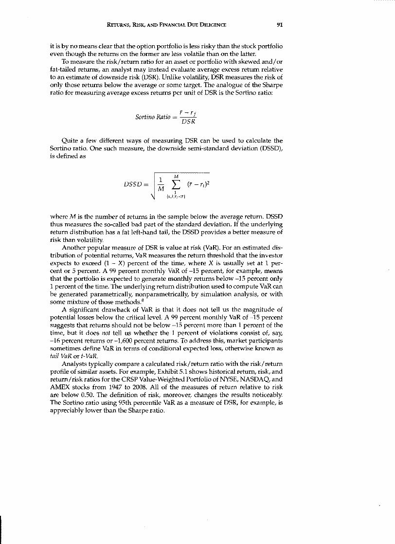
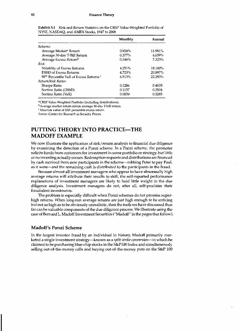
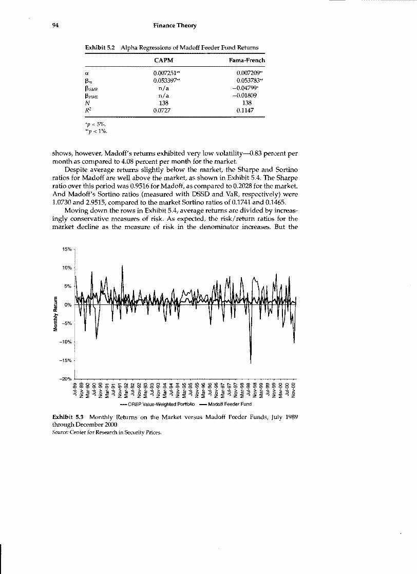
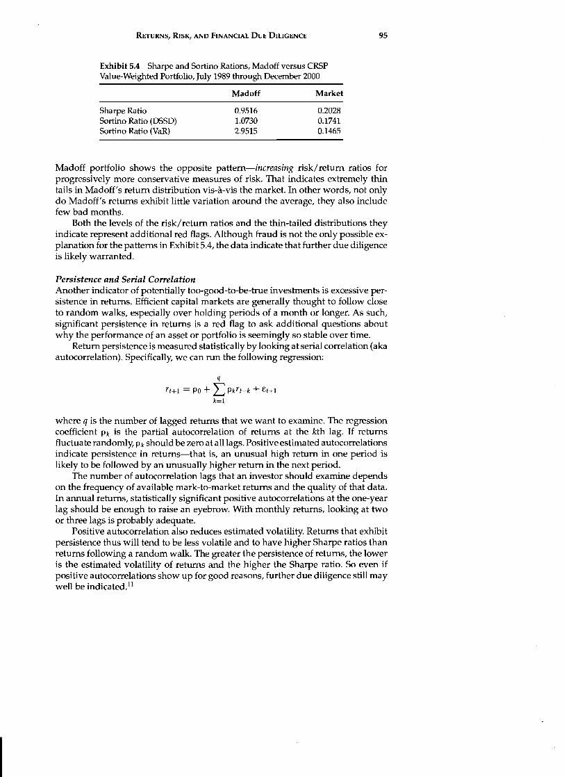
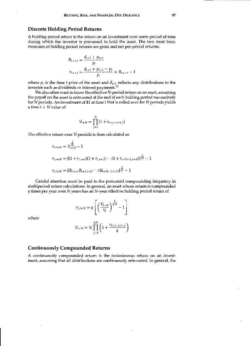
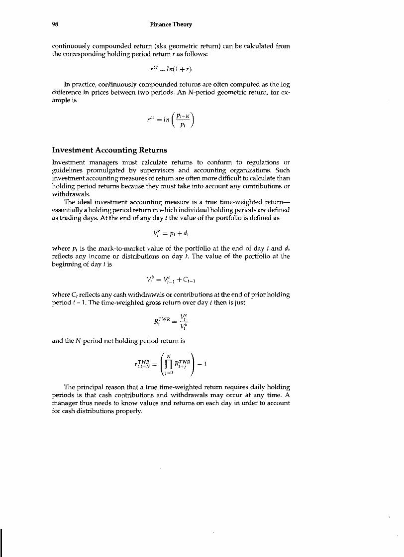