ISSN 2042-2695

CEP Discussion Paper No 1190

February 2013

Moving Up and Sliding Down:

An Empirical Assessment of the Effect of

Social Mobility on Subjective Wellbeing

Paul Dolan and Grace Lordan

Abstract Many people remain in the same income group as their parents and this is a cause of much discussion

and some concern. In this work, we examine how intergenerational mobility affects subjective

wellbeing (SWB) using the British Cohort Study. Our SWB measures encapsulate life satisfaction and

mental health. We find that relative income mobility is a significant predictor of life satisfaction and

mental health whether people move upward or downward. For absolute income, mobility is only a

predictor of SWB and mental health outcomes if the person moves downward. We also explore

pathways through which income mobility can impact on these outcomes. In particular, we present

evidence that suggests much of the effect of income mobility on SWB is due to changes in the

perception of financial security. But those who slide down are still less satisfied with their lives over

and above any effect of financial insecurity. Overall, there is an asymmetric effect of income

mobility: the losses of sliding on down are larger than the gains of moving up.

Keywords: income mobility, social mobility, inter-generational, life satisfaction, SWB, subjective

wellbeing, mental health

JEL Classifications: D31; D63; I1; I14; J60;

This paper was produced as part of the Centre’s Wellbeing Programme. The Centre for Economic

Performance is financed by the Economic and Social Research Council.

Acknowledgements We are grateful for the comments received from the wellbeing group at the CEP in the LSE, the

Social Policy seminar series at the LSE, the ESRI seminar series, the HEDG group at York and the

Health Methodology Research Group at Manchester. We are particularly grateful (in no particular

order) to comments received from Robert Havemann, David Johnston, Paul Frijters, Andrew Clarke,

Richard Layard, Stephen Jenkins, Nick Powdthavee, Anne Nolan, Andrew Jones, Nigel Rice, Julian

Le Grand, Mike Murphy, Ernestina Coast, Robert Metcalfe, George Kavetsos, Laura Kudrna,

Francesca Cornaglia, Alex Thompson and Tessa Peasgood. Financial support from the UK

Department for Work and Pensions and US National Institute on Aging (Grant R01AG040640) is

gratefully acknowledged.

Paul Dolan is an Associate of the Centre for Economic Performance and Professor of

Behavioural Science in the Department of Social Policy at the London School of Economics and

Political Science. Grace Lordan is an Associate of the Centre for Economic Performance and Lecturer

in Health Economics in the Department of Social Policy, London School of Economics and Political

Science.

Published by

Centre for Economic Performance

London School of Economics and Political Science

Houghton Street

London WC2A 2AE

All rights reserved. No part of this publication may be reproduced, stored in a retrieval system or

transmitted in any form or by any means without the prior permission in writing of the publisher nor

be issued to the public or circulated in any form other than that in which it is published.

Requests for permission to reproduce any article or part of the Working Paper should be sent to the

editor at the above address.

P. Dolan and G. Lordan, submitted 2013

  2  

Inter-generational income mobility affects life satisfaction and mental health- doing worse than your parents hurts more than doing better

1. Introduction

Social mobility is severely limited in the UK and elsewhere (Ermisch, Francesconi,

and Siedler 2006; Jo Blanden, Gregg, and Macmillan 2007) and this raises concerns

about inequalities of opportunity. Most recently, the Milburn (2012) report suggests

that opening the doors to a university education is the only way to advance social

mobility. Many papers have considered the effects of mobility on objective outcomes,

such as employment, but fewer have considered the effects on reports of subjective

wellbeing (SWB) and health. SWB is gaining prominence in academic and policy

circles (Dolan and Metcalfe 2012) and so the time is right to consider

intergenerational mobility and SWB. In this paper, we consider how social mobility

affects SWB, with SWB being measured as either changes in life satisfaction or

mental health. We consider three different measures of income mobility.

There is a large literature that looks at how relative income affects SWB (Dolan,

Peasgood, and White 2008; Bechtel, Lordan, and Rao 2012). The main message is

that SWB is adversely affected if you are surrounded by people who are richer than

you. Relative income has been measured in a host of ways but usually the comparison

group is people of a similar age and gender at a given point in time (Knight and Song

2006; Luttmer 2005; Card et al. 2010; Li et al. 2011; Senik 2004). That is, people

‘like me’. This may reflect a theoretical suggestion that relative position enters the

utility function directly (see Clark and Oswald (1998), for example) or it may simply

reflect data availability.

Alternatively, the comparison group could be the income that the individual

experienced in the past. This accommodates the notion that people feel changes in

income more intensely than absolute levels of income (Rabin 2004). Where

comparisons with past income have been considered, it has been usual to consider the

income that the individual themselves has earned in the recent past. To our

knowledge, the impact of inter-generational income mobility has yet to be considered

with respect to SWB or health.

  3  

Two papers have considered different measures of inter-generational mobility. First,

Clark and D’Angelo (2009) look at how upward class mobility affects SWB by using

15 waves of the BHPS. They find that individuals with greater mobility have higher

levels of life satisfaction. Their scope is more limited than our work as they only

consider upward mobility, defined as a binary indicator. Second, McBride (2001)

utilises the answer to the following question to create an inter-generational measure of

mobility: “compared to your parents when they were the age you are now, do you

think your own standard of living now is: much better, somewhat better, about the

same, somewhat worse, or much worse?” The author finds that respondents who

perceive their parents as having a higher standard of living in comparison to their own

report lower levels of well-being. This study is limited, however, in its cross sectional

nature and by the fact that the respondent is asked to recall their parents’ standard of

living.

In this work, we explore both upward (positive) and downward (negative) income

mobility. We use the British Cohort Study (BCS) to show how income mobility

affects life satisfaction and mental health. In what follows, the next section outlines

the conceptual framework for our analysis. Section 3 details the data used in this

work, our definitions of income mobility and our methodology. Section 4 presents our

results. The paper concludes with a discussion in section 5.

Overall, we find that relative income mobility is a significant predictor of life

satisfaction and mental health. Only downward absolute income mobility is a

predictor of these outcomes. We present analysis to highlight that variation in

consumption patterns and perception of financial situation may be viable pathways

through which our mobility effect operates. Crucially, our results are robust to a

number of specifications, including those that utilise a lagged dependent variable.

2. Conceptual Framework

2.1 Income mobility and SWB

  4  

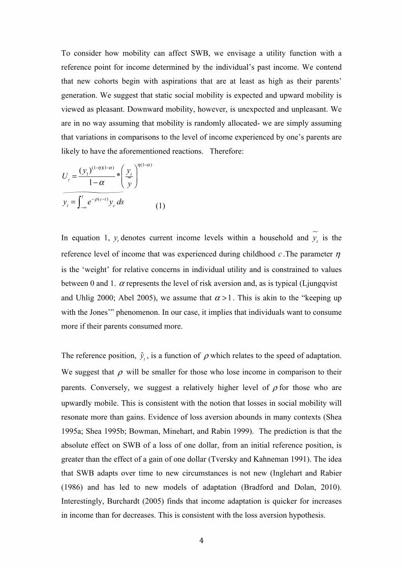
To consider how mobility can affect SWB, we envisage a utility function with a

reference point for income determined by the individual’s past income. We contend

that new cohorts begin with aspirations that are at least as high as their parents’

generation. We suggest that static social mobility is expected and upward mobility is

viewed as pleasant. Downward mobility, however, is unexpected and unpleasant. We

are in no way assuming that mobility is randomly allocated- we are simply assuming

that variations in comparisons to the level of income experienced by one’s parents are

likely to have the aforementioned reactions. Therefore:

Ut =(y1)

(1!! )(1!! )

1!!*yty!

"

#$%

&'

! (1!! )

yt = e!! (c!t ) yc ds!(

t

)!

(1)

In equation 1, ty denotes current income levels within a household and yt!

is the

reference level of income that was experienced during childhood c .The parameter η is the ‘weight’ for relative concerns in individual utility and is constrained to values

between 0 and 1. α represents the level of risk aversion and, as is typical (Ljungqvist

and Uhlig 2000; Abel 2005), we assume that 1α > . This is akin to the “keeping up

with the Jones’” phenomenon. In our case, it implies that individuals want to consume

more if their parents consumed more.

The reference position, !yt , is a function of ρ which relates to the speed of adaptation.

We suggest that ρ will be smaller for those who lose income in comparison to their

parents. Conversely, we suggest a relatively higher level of ρ for those who are

upwardly mobile. This is consistent with the notion that losses in social mobility will

resonate more than gains. Evidence of loss aversion abounds in many contexts (Shea

1995a; Shea 1995b; Bowman, Minehart, and Rabin 1999). The prediction is that the

absolute effect on SWB of a loss of one dollar, from an initial reference position, is

greater than the effect of a gain of one dollar (Tversky and Kahneman 1991). The idea

that SWB adapts over time to new circumstances is not new (Inglehart and Rabier

(1986) and has led to new models of adaptation (Bradford and Dolan, 2010).

Interestingly, Burchardt (2005) finds that income adaptation is quicker for increases

in income than for decreases. This is consistent with the loss aversion hypothesis.

  5  

In this work, we explore inter-generational upward and downward mobility. We see

four pathways that are not mutually exclusive through which mobility can affect SWB

and health. These are: i) stress ii) prosperity concerns iii) identity and iv) consumption

changes.

For our first pathway, we envisage individuals fully internalizing their new status and

gaining a ‘feeling of pride’ when they are mobile and a ‘feeling of ‘dispair’ when they

are dis-mobile.

Our second pathway is similar but the positive and negative effects on SWB are

attributed solely to the gains and losses in prosperity. This hypothesis is consistent

with a literature that highlights that poorer perceptions of one’s current financial

situation are associated with lower SWB and that perceptions of change in financial

circumstances affect well-being (Wildman and Jones 2002; Brown, Taylor, and

Wheatley Price 2005; Johnson and Krueger 2006). For both pathways, SWB and

mental health will be affected mainly through increased or decreased stress levels.

Johnston and Lordan 2012 document the mechanisms by which stress can affect SWB

and overall health. These stress effects can be subsequently augmented, as individuals

who report low SWB are also less likely to commit to the future and be optimistic. As

a consequence, they may be less likely to pursue healthy lifestyle activities such as

regular exercise and managing a nutritious diet. They may also choose to engage in

risky health-behaviours such as excessive drinking and smoking (Macinko et al.

2003). This is also akin to status anxiety (Wilkinson and Pickett 2009; Botton 2005).

For individuals who are mobile, there is likely to be an alleviation of stress as they

move from a situation with less disposable income (and vice versa for the

downwardly mobile). This change therefore has the potential to augment (worsen)

their SWB.

Our third pathway is the identity hypothesis which stems from evidence that changing

comparison groups, such as when there is mobility, can affect an individual’s sense of

identity (Akerlof and Kranton 2010). All animals, including human ones, need to feel

that they belong to a group, and changing social classes, even in a supposedly good

way, can result in an individual neither feeling part of their former group nor part of

  6  

their new group. This process is used to explain why children from poor backgrounds

who win scholarships are not as happy as their equally high achieving peers from

more affluent backgrounds (Aries and Seider 2005). In our case, an identity loss can

potentially affect both the upwardly and downwardly mobile if the person no longer

socializes with old friends and family members regularly.

Our fourth pathway, consumption changes, suggests that individuals may not fully

realise the utility (disutility) of their new income status. If true, individuals who are

upwardly income mobile consume less. This may occur because these individuals do

not feel secure in their newfound status and want to ensure they can smooth future

consumption. Additionally, they are likely to have less permanent income in the sense

that they may have a lower likelihood of having an inheritance. Finally, having grown

up in a lower income environment, they may not view themselves as needing the

same level of consumption as those who have grown used to it. This actually suggests

that individuals who are mobile are slow to adapt. Conversely, downward mobility

may impact SWB and health if individuals still spend in accordance with the

reference group of their childhood. It follows that they worry about their financial

situation (our first pathway) and also consume more.

3. Data and methods

This work utilises the 1970 British Cohort Study (BCS70). The BCS70 began by

including more than 17,000 births between April 5-11 in 1970. It is estimated that

these births represent more than 95% of births over these days in England, Scotland,

Wales and Northern Ireland. Currently data are available for eight major follow-up

surveys: 1975, 1980, 1986, 1991, 1996, 2000, 2004 and 2008. Added to the three

major childhood surveys (age 5, 10 and 16) are any children who were born outside of

the country during the week of April 5-11 and could be identified from school

registers at later ages. We are using this data as it is one of the few data sets that have

the information required to consider inter-generational mobility.

3.1 Income Mobility Measures

This work focuses on the impact of income mobility as defined by changes in

  7  

household income from ages 10 (1980) through age 30 (2000) and age 34. Age 10 is

chosen, as it is the earliest year that income information was gathered from the BCS

families. The response rate in 1986 is also lower. In 1980, income represents the gross

income of the child’s mother and father and is reported in bands  (please see Appendix

A, A.1).

Ages 30 and 34 are chosen as they are deemed ages when a person is likely to be

settling into their income level. They are also the years when the most questions were

asked regarding health and life satisfaction. Considering two different time points is

important for two reasons. First, for some careers (for example, an academic who is

tenure tracked) a person may not have settled into a particular income by age 30.

Second, a person who finds they are doing better/worse than their parents at age 30

may have SWB and health gains/losses at that time but adapt as they realize their

gains/losses are permanent. That is, they find satisfaction in some other life

dimension. As in the case of the 1980 questionnaire, our measure of income for 2000

and 2004 represents household income. Here it is defined as the net weekly combined

income of the BCS child and their partner (if applicable). As in 1980 it excludes any

income of household members and child benefits.

Using multiple years of income in adulthood helps abate concerns that income

gathered in a ‘one snapshot’ fashion is not a good measure of permanent income. It is,

however, worth noting that for surveys like these the correlation between current

income and permanent income is quite strong (0.74) (Blanden, Gregg, and Macmillan

2011). The first difficulty in defining income mobility surrounds how it should be

calculated. An obvious way to proceed would be to take the difference of adult

income minus child income but the mobility measure would then be perfectly multi-

collinear with the adult income and child income variables that we include in our

equation. That is, we would need to assume that either adult income or childhood

income have no effect on SWB. This is an unrealistic assumption. Our work defines

income mobility in different ways. While it seems obvious that if you do worse than

your parents financially, your SWB will suffer owing to dips in standard of living but

it could be that relative and/or absolute changes in income matter.

We therefore consider three measures of mobility that circumvent this problem. These

  8  

are two measures of relative mobility and one measure of absolute mobility. Our first

relative measure of mobility is defined as the intergenerational movement between

income quintiles. This allows us to overcome the problem of income being reported

as bands at age 10. A person is defined as upwardly mobile if they moved upward at

least one quintile from their parents’ household income in 1980 to their own income

quintile in 2000. Conversely, a person is defined as downwardly mobile if they moved

downward at least one income quintile from their own parent’s income in 1980. We

rely on the Family Expenditure Survey to define our income quintiles given that

attrition in 1980 is likely to be non-random in the BCS. We do this given the criticism

that cohort studies tend to underestimate income for most of the income distribution

in the BCS (Blanden, Gregg, and Macmillan 2011). This is in comparison to the

Family Expenditure Surveys (FES) of the same year, which contain more detailed

information. For 1980, the relevant income quintiles were drawn from the same year’s

data sets based on the variable representing gross normal household income. For 2000

and 2004, the relevant income quintiles were defined based on the disposable income

deciles reported in the Office of National Statistics reports of the same surveys. Along

with circumventing an attrition problem, we view that this also overcomes the

limitations of income being reported in gross form in childhood surveys but as net in

recent years. Full details of how the quintiles were derived can be found in Appendix

A, A.2.

Our second measure of relative income mobility is based on percentile change in

income inter-generationally and is defined internally based on incomes reported at

ages 10, 30 and 34 within the BCS data. In this respect, it has the limitations on being

based on a sample that may be biased by attrition; however, it has the advantage of

retaining more information. That is, our first measure may also be biased by dubbing

an individual as ‘mobile’ if they are sitting on the edge of a quintile between two time

periods. This measure is derived by first calculating the difference between the BCS

child’s income in percentiles minus their parent’s income in percentiles.

Subsequently we create two variables to capture upward mobility and downward

mobility. Upward mobility is defined as equal to this difference if it is positive and

zero otherwise, and vice versa for downward mobility. Further details of these

calculations are provided in Appendix A.3.

  9  

Our final measure is concerned with absolute movements in income inter-

generationally. It is defined as the difference between adult and childhood income

divided by childhood income. Because the income bands reported in 1980 relate to

gross income, it is necessary to calculate an approximation of what the take home pay

would have been. To do this, we convert the mid-points of the 1980 income bands

into 2004 GBP. Next, we calculate what the weekly take home pay would have been

given the average tax rules of the 2004/2005 tax year. For the 2000 differences we use

the same values and therefore convert weekly income at age 30 into 2004 values.

Further details of these calculations are provided in Appendix A.4. For values that are

greater than zero, we create a variable defined ‘upwardly’ mobile, that is zero

otherwise. For values that are less than zero, we create a variable defined

‘downwardly’ mobile that is zero otherwise.

3.2 SWB Outcomes

Our main analysis considers how inter-generational income mobility between 1980

and 2000/2004 affects SWB. The measure of SWB is based on a life satisfaction

question that takes a value from 0 to 10 where 10 is the highest level of satisfaction. It

is available at ages 30 and 34. Specifically, it is the response to the following

question: “Here is a scale from 0-10 where '0' means that you are completely

dissatisfied and '10' means that you are completely satisfied. Please enter the number,

which corresponds with how satisfied or dissatisfied you are about the way you life

has turned out so far”.

Our first measure of mental health is the Rutter Malaise Inventory (Rutter, Tizard, and

Whitmore 1970), which is a set of questions that combine to measure levels of

psychological distress or depression. At age 30, its scores range from 0 to 24, with

each question scoring a value of 1. Specifically, the index is derived through the

number of yes scores to: having backaches, feeling tired, feeling miserable and

depressed, having headaches, worrying, having difficulty in falling asleep or staying

asleep, waking unnecessarily early in the morning, worrying about health, getting into

a violent rage, getting annoyed by people, having twitches, becoming scared for no

reason, being scared to be alone, being easily upset, being frightened of going out

alone, being jittery, suffering from indigestion, suffering from upset stomach, having

  10  

poor appetite, being worn out by little things, experiencing racing heart, having bad

pains in your eyes, being troubled by rheumatism, and having had a nervous

breakdown. For age 34, only nine of the questions usually asked in the Rutter Malaise

Inventory were included. Specifically, we derive a sub-malaise index by aggregating

the number of yes responses to: feeling tired, feeling miserable and depressed,

worrying, getting into a violent rage, becoming scared for no reason, being scared to

be alone, being easily upset, being jittery, suffering from indigestion, suffering from

upset stomach, having poor appetite, being worn out by little things, experiencing

racing heart.

We also measure mental health using the 12-item version of the General Health

Questionnaire (GHQ) at age 30. The GHQ is a commonly used self-reported measure

of mental health and consists of questions regarding the respondent’s emotional and

behavioural health over the past few weeks. The 12 items in the GHQ are: ability to

concentrate, sleep loss due to worry, perception of role, capability in decision making,

whether constantly under strain, problems in overcoming difficulties, enjoyment of

day-to-day activities, ability to face problems, whether unhappy or depressed, loss of

confidence, self-worth, and general happiness. For each of the 12 items, the

respondent indicates on a four-point scale the extent to which they have been

experiencing a particular symptom. For example, the respondent is asked ‘have you

recently felt constantly under strain’, to which they can respond: not at all (a score of

0), no more than usual (1), rather more than usual (2), much more than usual (3). We

use the respondents’ total response as our mental health measure.

The GHQ is not available at age 34 but this survey did include four questions usually

included in the Kessler scale. The Kessler scale is usually featured as a 6 item or more

normally as a 10-item questionnaire (Kessler et al. 2002). We follow the same method

here used to aggregate the 10-item index but flag that this is not the usual Kessler

index that is seen in the literature. The specific questions asked are during the last 30

days, about how often did you feel i) so depressed that nothing could cheer you up? ii)

hopeless? iii) restless or fidgety? iv) that everything was an effort? The possible

responses are: all of the time (a score of 1), most of the time (2), some of the time (3),

a little of the time (4) and none of the time (5). This results in an index that has a

range between 4 and 20, with 4 being the best outcome with respect to mental health.

  11  

We estimate the effect of social mobility on SWB in the first instance by ordinary

least squares (OLS) using the three definitions of income mobility described above.

Estimating this effect is complicated by the need to control for current adult income

and childhood income, whereby the latter captures some aspects of childhood

variables. Specifying upward and downward mobility as dummy variables allows us

to control for both of these income types. Therefore, we estimate:

1 1980 1 1980 1980' 'it t t adult iOutcome UP DOWN x yβ α γ χ ε− −= + + + + (2)

 Here i indexes the BCS child and t indicates either age 30 or aged 34. UPt!1980

denotes upward social mobility and DOWNt!1980 denotes downward social mobility.

As discussed we consider three definitions of income mobility. x is a vector of

childhood variables. These are: household weekly income, birth weight, gender,

maternal education (indicators as to whether she has a degree, a vocational

qualification, ‘A’ levels, ‘O’ levels, a trade qualification or ‘other’ qualification),

mother’s age, maternal employment, fraternal education (consistent with the

definition of maternal education), father’s age, father’s employment, household size,

household size squared, tenure (lives in a rural area, lives in an urban area, lives in a

council estate, lives in a suburb, lives in ‘other’ area), number of younger siblings,

number of older siblings, region of birth, and a dummy indicating whether the child

had no father figure. For cases where mother education, father education, mother

employment, father employment, mother’s age, father’s age or household income are

missing dummies are created in order to not lose the data.

y denotes a vector of adult variables that can affect SWB and health which are taken

at age 30 or age 34 depending on the timing of the outcome of interest. These are

weekly household income at age 30, social class (a set of fixed effects that denote one

of the six registrar general social classes), marital status (disaggregated into fixed

effects representing married, cohabiting, single and separated/divorced/widowed),

whether or not the BCS child has a degree, household size and household size

squared.

  12  

4. Results

The OLS results pertaining to equation 2 are documented in Table 1 for relative

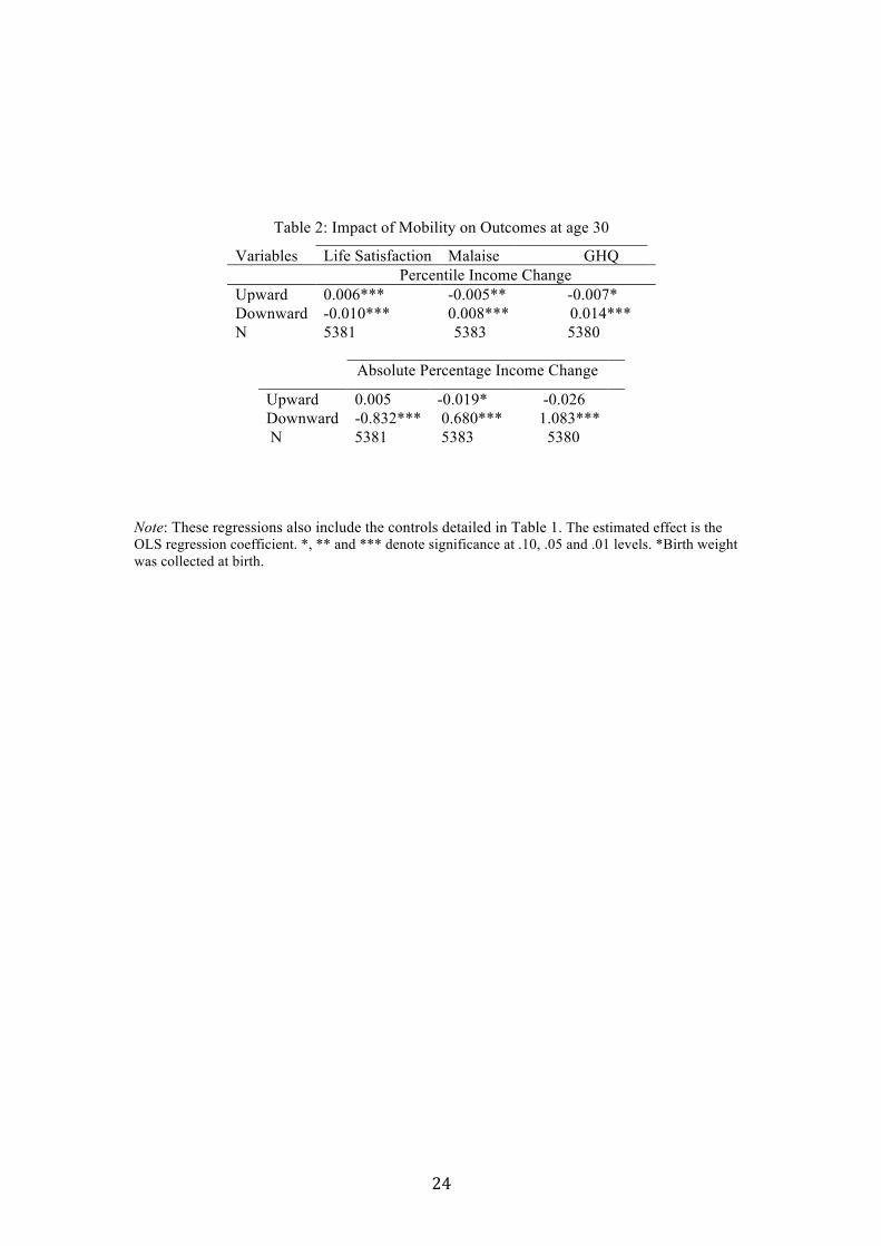
income mobility at age 30, where we also document our control variables. Table 2

documents the results for our second measure of relative income mobility (percentile

based) at age 30. We choose to focus on OLS as the coefficients are readily

interpretable but using ordered probits for the life satisfaction equations does not

change our overall conclusions. All our standard errors are robust and *, **, ***

denote significance at the 10%, 5% and 1% levels respectively. Overall the main

results of our work can be found in Tables 1 through 4, with an overall summary in

Table 5.

From Table 1, we can see that very few of our childhood variables affect our SWB

outcomes. For all outcomes, childhood income at age 10 is highly important, perhaps

representing early childhood investments rather than income per se. Tenure type is

also associated with varying levels in life satisfaction. Adult variables matter more.

Social class is associated with variation in life satisfaction and mental health in the

direction we would expect. Household weekly income is also a predictor of higher

SWB and better mental health. Relationships are also associated with better SWB and

mental health, with those who are married or co-habiting being better off than others.

Considering relative income mobility measured as quintile changes, upward mobility

positively predicts life satisfaction and mental health. The magnitude of the

coefficients are large and consistent with the loss aversion hypothesis, downward

mobility hurts more. Turning to Table 2, for relative income mobility based on

changes in the income percentile distribution, income mobility yields gains to SWB

and mental health whilst downward mobility deteriorates these outcomes. This is

consistent with the conclusions from Table 1 emanating from our quintile-based

measure of relative mobility. The results for absolute mobility highlight a different

story. That is, inter-generational movements in absolute income only affect SWB and

mental health if they are downward.

Table 3 is in the same format as Table 1 and shows the outcomes at age 34. We again

  13  

document our full set of controls, which follow a similar pattern to that described for

Table 1. For relative income mobility based on quintile changes, the results that are

directly comparable with Table 1 are those pertaining to life satisfaction. For life

satisfaction, the associations in Table 3 are lower, implying that inter-generational

mobility is less predictive of life satisfaction at age 34 than at age 30. It is therefore

possible that we are seeing an adaptation process that is incomplete. The malaise

index at age 34 is lower for those who are upwardly mobile. The results for the

Kessler scale suggest that those who are upwardly mobile are significantly better off,

whereas those who are downwardly mobile do worse.

Turning to Table 4, considering relative income mobility based on percentile income

change, the conclusion is similar to that found at age 30: both upward and downward-

mobility predict SWB and mental health. The exception here is that the coefficient on

upward mobility for the malaise score is no longer significant. Comparing the

coefficients for life satisfaction, the results for both upward and downward mobility at

ages 30 (Table 2) and 34 (Table 4) are relatively stable. Therefore, we do not have

evidence of adaptation to mobility over the four years we observe.

Table 4 shows the results for our absolute mobility measure. As was the case for

SWB outcomes at age 30, the only associations are for downward absolute income

mobility. For life satisfaction the size of the coefficient is larger at age 34 in

comparison to age 30, suggesting that individuals do not adapt to absolute income

mobility if it is downward. The deterioration to the malaise index and the Kessler

scale is also large for those age 34 implying that being downwardly mobile in

absolute terms is a predictor of SWB overall.

Table 6 presents results that allow us to explore some pathways through which

mobility affects SWB. Firstly, we explore whether our identity hypothesis may help

explain this phenomenon utilising data from the 2000 (aged 30) surveys on the BCS

child’s level of contact with their mother. Specifically, the BCS child is asked how

often they see their mother with the following options for response: i) more than once

a week ii) more than once a month and iii) less than once a month iv) never v) lives

with mother. The results under the heading ‘maternal contact regressions’ detail

results from regressions that add these five fixed effects to the model described in

  14  

equation 2. Two things are worth noting. Firstly, maternal contact does not seem to be

an important predictor of SWB outcomes. Secondly, while in most cases the impact of

mobility – both relative and absolute – is reduced, this reduction is small and does not

over-ride the overall conclusions evident from Tables 1 through 4.

The section of Table 6 labelled ‘prosperity regressions’ considers prosperity concerns

as a pathway through which inter-generational income mobility affects SWB and

mental health. To do this, we add to equation 2 a measure of perceived financial

prosperity at aged 30, taking values one through five, representing the response to the

question: ‘how well are you managing financially these days’. The options for the

respondent are: 1) living comfortably 2) doing alright 3) just about getting by 4)

finding it quite difficult or 5) finding it very difficult. We include this variable in

equation 2 as a set of fixed effects. From Table 5, we see that prosperity concerns are

a viable pathway through which income mobility is operating. In particular, upward

mobility is no longer a significant predictor of SWB and mental health. For all three

of our mobility measures, downward mobility is no longer a significant predictor of

mental health. Interestingly, for life satisfaction, downward mobility is still a

significant predictor of worse outcomes in all three cases. The size of the coefficients

is reduced, however, indicating that prosperity concerns were indeed a partial

pathway for the effect of downward mobility.

Realised and unrealized consumption changes may be an alternative pathway through

which mobility affects SWB. We can explore this by using the fact that, if individuals

are consuming less, they are likely to be saving more. Using information on savings

habits gathered at age 34, we add two variables to equation 2 when considering

outcomes at this age. That is, we add: i) an indicator (yes/no) for if the child saved

monthly; and ii) how much the child saves monthly. The results from these

regressions are shown in Table 6 under the heading ‘savings regressions’. For relative

income mobility based on quintile changes, adding these variables renders the

predictive power of upward mobility not significant. For downward mobility based on

the same measure, the coefficients associated with all outcomes are reduced, however,

for life satisfaction and our Kessler sub index the effects remain significant. The

impact of upward and downward mobility based on relative changes in percentiles is

still a predictor of SWB in all cases with the exception of the sub malaise indictor. For

  15  

absolute income mobility, the significant impact of downward mobility remains for

all outcomes at the 1% level.

Our work has documented a persistent and strong relationship between income

mobility- both relative and absolute- and a variety of health outcomes. The pertinent

question now is whether or not this is a causal relationship. That is, it is feasible that

some of this relationship is determined by characteristics of the individual that makes

them more likely to be mobile (for example, being the proverbial black sheep) and

also report a certain level of SWB or health. Additionally, it is likely that there may

be personality factors correlated with the reporting a certain level of health or SWB

and the likelihood of being mobile. In order to consider this we include some

measures that are likely to capture personality. That is, we include an index of

emotional and behavioral problems at age 10 and age 16. These indexes are often

labeled as non-cognitive skills (Heckman 2008) and are based on the Rutter

behavioral problems index. Additionally, for two of the outcomes we consider it is

possible to add a lagged dependent variable. These are life satisfaction and health

which we observe with a lag of four years (that is, at age 26 for the age 30 outcomes

and at age 30 for the age 34 outcomes). We argue that including a lagged dependent

variable should over control for negative ‘feelings’ associated with being mobile as its

information was gathered at a time when the BCS child would have had some

knowledge of their income attainment in comparison to their parents. Additionally,

assuming that the tendency to report a certain level of health or life satisfaction does

not change in a four-year period than this approach also handles this concern. The

results for life satisfaction and health are documented in Table 7.

From Table 7, considering the results that control for behavior at age 10 (under

heading ‘behaviour results’), the overall conclusions of Tables 1 through 4 still hold-

that is, relative income mobility-either based on quantile or percentile change- both

upward and downward significantly predicts health and SWB, whereas for absolute

mobility only downward mobility matters. Adding a lagged dependent variable in the

health equation, when considering upward mobility, relative mobility is still a

predictor of health status at age 30 when measured using changes in percentiles. It is

only at age 34 that downward mobility, measured using absolute income changes, is a

predictor of health. The results for life satisfaction are more consistent across

16  

definitions of mobility once we include the lagged dependent variable. For upward

mobility, consistent with Tables 3 and 4, upward relative mobility, however

measured, significantly predicts life satisfaction at 30. This effect is not significant at

age 34 when relative mobility is measured based on changes in quantiles, but remains

significant when it is measured based on percentiles. Regardless of how we measure

downward mobility it is always a negative predictor of life satisfaction at ages 30 and

34.

This work has considered two ways to measure income mobility, however the data at

our disposal does have a measure of social class- the Registrar Generals division of

individuals into six social classes. Utilising this information we re-create Table 1 and

3 with respect to social class mobility. The results for upward and downward mobility

are documented in Table 8. We do however present these results with caution. Unlike

our income mobility estimates, which control for both child income and adult income,

we cannot control for child and adult social class. This problem arises owing to multi-

collinearity. Therefore, the results in Table 8 only contain adult social class (which we

document). Overall, this Table suggests that social class mobility of this definition

worsens health, regardless of whether it is upward or downward.

5. Discussion

Many people remain in the same social class as their parents and this is a cause of

much discussion and some concern. In this work, we examine how intergenerational

mobility affects life satisfaction and mental health using the British Cohort Study. We

define mobility as income movements inter-generationally both relatively and

absolutely. We define relative mobility based on changes in quintiles and percentiles.

The advantage of the former is that the quintiles are derived based on external data

that arguably better represents the income distribution in the UK of that time, whereas

the latter allows for greater numbers of individuals to be ‘winners’ and ‘losers’ We

find that relative income mobility is a significant predictor of life satisfaction and

mental health. We also find that its effects are consistent with the loss aversion

hypothesis – going down matters more. This is reflected in the fact that the

coefficients attached to downward mobility are always larger than those for upward

mobility. Our measure of absolute income mobility is only a predictor of SWB if the

  17  

person moves down. Again, this suggests that a negative life event is felt more than a

positive life event. These conclusions are consistent whether we look at outcomes at

age 30 or 34. Taken together, our results suggest an asymmetric effect of inter-

generational income mobility on SWB.

We proposed four pathways through which mobility can affect life satisfaction and

mental health: i) stress/alleviation of stress; ii) prosperity concerns; iii) changes in the

sense of identity; and iv) realised or unrealised consumption changes. We do not have

data to explore whether i) is a viable pathway. For the prosperity pathway, using data

on financial concerns, we find it a viable pathway for our mobility affects. In

particular, after adding these regressors mobility is no longer a significant predictor of

mental health but its association with life satisfaction remains and it is large. Taken at

face value, this seems to imply that only financial stress really matters for mental

health when it comes to mobility. Interestingly, the effect of upward mobility on life

satisfaction is also not significant. This suggests that it is the feeling of financial

security that drives life satisfaction gains for the upwardly mobile and that the feeling

of ‘pride’ associated with moving up in the world does not give long term life

satisfaction gains.

Overall, we find that the identity hypothesis is not an important pathway. We do

acknowledge, however, that maternal contact is a crude measure of identity and

ideally we would have information on changes to social networks. Finally, for

realised and unrealised consumption, we find that savings is a probable pathway for

our mobility affects. This finding echoes the importance of research considering

consumption data rather than income when exploring the effects of windfalls on

SWB.

Clearly, individuals are not randomly assigned to a mobility status and these values

describe an association rather than a cause and effect. We have tested the sensitivity

of our results to controlling for non-cognitive skills at age 10 and a lagged dependent

variable in our life satisfaction models. The conclusions documented here are stable to

the addition of these variables. That is, relative income mobility (both upward and

downward measured using either quintile or percentile changes) significantly predicts

life satisfaction, whereas for absolute mobility only downward mobility matters.

  18  

Given that the life satisfaction lagged measure we incorporate was likely to have been

taken amidst a downward income spiral, we view these estimates as a lower bound of

the effect of downward mobility on life satisfaction. Clearly, unambiguous proof of a

casual effect of social mobility requires data does not exist.

We also consider how social mobility measured using the Registrar Generals

framework affects our health outcomes. We do not find any significant associations

between class mobility and SWB. This is in contrast with the results found by Clark

and D’Angelo (2009); however, we do note that they identify effects of upward class

mobility from a comparison with all others. In this case, ‘others’ includes those who

are downwardly mobile. Additionally, the authors use the Hope and Goldthorpe

framework for social class. This is a far more detailed measure of mobility and is

currently beyond the data that is available to us.

A natural question arising from our work is how income mobility should be measured

to best capture how a person decides if they are doing better or worse than their

parents. The answer is that we do not know. We do however, believe that children do

compare themselves to their parents. Additionally, the results we present should

convince our audience that children make these comparisons based on income and

some notion of changes in standard of living.

We are more circumspect in saying anything about the policy recommendations of

this research because it raises many normative issues about how to appropriately

weigh the many factors that go into the conceptualisation and derivation of the social

welfare function. Firstly, it should be noted that income at ages 30 and 34 is also a

significant predictor of SWB. Therefore, to the extent that you would like the world to

remain equitable with respect to who gets this income effect, there is an argument to

promote mobility. Secondly, as it has been noted many times, mobility in the UK is

limited. This in itself affects the likelihood of finding significant mobility effects.

Lastly, much of the deterioration of SWB can be explained by prosperity concerns

and a lack of saving for the downwardly mobile that are larger than others

experiencing the same level of income. This suggests that there might be a role for

policy in helping people to stop living beyond their means that can mitigate some of

the effects found here.

  19  

References:

Abel,  A.  B.  2005.  “Optimal  Taxation  When  Consumers  Have  Endogenous  Benchmark  Levels  of  Consumption.”  The  Review  of  Economic  Studies  72  (1):  21–42.  

Akerlof,  George  A.,  and  Rachel  E.  Kranton.  2010.  Identity  Economics:  How  Our  Identities  Shape  Our  Work,  Wages,  and  Well-­‐Being.  Princeton  University  Press.  

Aries,  E.,  and  M.  Seider.  2005.  “The  Interactive  Relationship  Between  Class  Identity  and  the  College  Experience:  The  Case  of  Lower  Income  Students.”  Qualitative  Sociology  28  (4):  419–443.  

Bechtel,  L.,  G.  Lordan,  and  D.  S.  Rao.  2012.  “Income  Inequality  And  Mental  Health—Empirical  Evidence  From  Australia.”  Health  Economics  21:  4–17.  

Blanden,  J.,  P.  Gregg,  and  L.  Macmillan.  2011.  “Intergenerational  Persistence  in  Income  and  Social  Class:  The  Impact  of  Within-­‐group  Inequality.”  http://papers.ssrn.com/sol3/papers.cfm?abstract_id=1976533.  

Blanden,  Jo,  Paul  Gregg,  and  Lindsey  Macmillan.  2007.  Accounting  for  Intergenerational  Income  Persistence:  Noncognitive  Skills,  Ability  and  Education.  Forschungsinstitut  zur  Zukunft  der  Arbeit.  

Botton,  Alain  de.  2005.  Status  Anxiety.  Penguin  UK.  Bowles,  Samuel,  Herbert  Gintis,  and  Melissa  Osborne  Groves.  2005.  Unequal  

Chances:  Family  Background  and  Economic  Success.  Princeton  University  Press.  

Bowman,  D.,  D.  Minehart,  and  M.  Rabin.  1999.  “Loss  Aversion  in  a  Consumption–savings  Model.”  Journal  of  Economic  Behavior  &  Organization  38  (2):  155–178.  

Bradford,  W.  D.,  and  P.  Dolan.  2010.  “Getting  Used  to  It:  The  Adaptive  Global  Utility  Model.”  Journal  of  Health  Economics  29  (6):  811–820.  

Brown,  S.,  K.  Taylor,  and  S.  Wheatley  Price.  2005.  “Debt  and  Distress:  Evaluating  the  Psychological  Cost  of  Credit.”  Journal  of  Economic  Psychology  26  (5):  642–663.  

Burchardt,  T.  2005.  “Are  One  Man’s  Rags  Another  Man’s  Riches?  Identifying  Adaptive  Expectations  Using  Panel  Data.”  Social  Indicators  Research  74  (1):  57–102.  

Card,  David,  Alexandre  Mas,  Enrico  Moretti,  and  Emmanuel  Saez.  2010.  Inequality  at  Work:  The  Effect  of  Peer  Salaries  on  Job  Satisfaction.  Working  Paper.  National  Bureau  of  Economic  Research.  http://www.nber.org/papers/w16396.  

Carroll,  C.  D.,  J.  Overland,  and  D.  N.  Weil.  1997.  “Comparison  Utility  in  a  Growth  Model.”  Journal  of  Economic  Growth  2  (4):  339–367.  

———.  2000.  “Saving  and  Growth  with  Habit  Formation.”  American  Economic  Review:  341–355.  

Clark,  A.,  and  E.  D’Angelo.  2009.  Upward  Social  Mobility,  Wellbeing  and  Political  Preferences:  Evidence  from  the  BHPS.  working  paper,  Paris  School  of  

  20  

Economics,  17  October.  http://jma2012.fr/fichiers2009/C5/clark_dangelo.pdf.  

Clark,  A.  E.,  P.  Frijters,  and  M.  A.  Shields.  2008.  “Relative  Income,  Happiness,  and  Utility:  An  Explanation  for  the  Easterlin  Paradox  and  Other  Puzzles.”  Journal  of  Economic  Literature  46  (1):  95–144.  

Clark,  A.  E.,  and  A.  J.  Oswald.  1994.  “Unhappiness  and  Unemployment.”  The  Economic  Journal:  648–659.  

———.  1998.  “Comparison-­‐concave  Utility  and  Following  Behaviour  in  Social  and  Economic  Settings.”  Journal  of  Public  Economics  70  (1):  133–155.  

Davey-­‐Smith,  G.  1996.  “Income  Inequality  and  Mortality:  Why  Are  They  Related?”  BMJ:  British  Medical  Journal  312  (7037):  987.  

Deaton,  Angus.  1992.  Understanding  Consumption.  Oxford  University  Press,  USA.  ———.  2003.  “Health,  Inequality,  and  Economic  Development.”  Journal  of  

Economic  Literature  41  (1)  (March):  113–158.  Dolan,  P.,  T.  Peasgood,  and  M.  White.  2008.  “Do  We  Really  Know  What  Makes  Us  

Happy?  A  Review  of  the  Economic  Literature  on  the  Factors  Associated  with  Subjective  Well-­‐being.”  Journal  of  Economic  Psychology  29  (1):  94–122.  

Dolan,  Paul,  and  Robert  Metcalfe.  2012.  “The  Relationship  Between  Innovation  and  Subjective  Wellbeing.”  Research  Policy  41  (8)  (October):  1489–1498.  doi:10.1016/j.respol.2012.04.001.  

Easterlin,  R.  A.  2004.  “The  Economics  of  Happiness.”  Daedalus  133  (2):  26–33.  Ermisch,  J.,  M.  Francesconi,  and  T.  Siedler.  2006.  “Intergenerational  Mobility  and  

Marital  Sorting*.”  The  Economic  Journal  116  (513):  659–679.  Graham,  C.,  and  S.  Pettinato.  2002.  “Frustrated  Achievers:  Winners,  Losers  and  

Subjective  Well-­‐being  in  New  Market  Economies.”  Journal  of  Development  Studies  38  (4):  100–140.  

Hayo,  Bernd,  and  Wolfgang  Seifert.  2003.  “Subjective  Economic  Well-­‐being  in  Eastern  Europe.”  Journal  of  Economic  Psychology  24  (3)  (June):  329–348.  doi:10.1016/S0167-­‐4870(02)00173-­‐3.  

Heckman,  James  J.  2008.  “Schools,  Skills,  and  Synapses.”  Economic  Inquiry  46  (3)  (June):  289.  

Huberman,  B.  A.,  C.  H.  Loch,  and  A.  Ön\ccüler.  2004.  “Status  as  a  Valued  Resource.”  Social  Psychology  Quarterly  67  (1):  103–114.  

Inglehart,  R.,  and  J.  R.  Rabier.  1986.  “Aspirations  Adapt  to  Situations—but  Why  Are  the  Belgians  so  Much  Happier  Than  the  French?  A  Cross-­‐cultural  Analysis  of  the  Subjective  Quality  of  Life.”  Research  on  the  Quality  of  Life.  Ann  Arbor:  Institute  for  Social  Research  University  of  Michigan.  

Johnson,  W.,  and  R.  F.  Krueger.  2006.  “How  Money  Buys  Happiness:  Genetic  and  Environmental  Processes  Linking  Finances  and  Life  Satisfaction.”  Journal  of  Personality  and  Social  Psychology  90  (4):  680.  

Johnston,  David  W.,  and  Grace  Lordan.  2012.  “Discrimination  Makes  Me  Sick!  An  Examination  of  the  Discrimination–health  Relationship.”  Journal  of  Health  Economics  31  (1)  (January):  99–111.  doi:10.1016/j.jhealeco.2011.12.002.  

Kessler,  R.  C.,  G.  Andrews,  L.  J.  Colpe,  E.  Hiripi,  D.  K.  Mroczek,  S.-­‐L.  T.  Normand,  E.  E.  Walters,  and  A.  M.  Zaslavsky.  2002.  “Short  Screening  Scales  to  Monitor  Population  Prevalences  and  Trends  in  Non-­‐specific  Psychological  Distress.”  Psychological  Medicine  32  (06):  959–976.  doi:10.1017/S0033291702006074.  

  21  

Knight,  J.,  and  L.  Song.  2006.  “Subjective  Well-­‐being  and  Its  Determinants  in  Rural  China.”  University  of  Nottingham.  http://www.csae.ox.ac.uk/conferences/2006-­‐eoi-­‐rpi/papers/gprg/knight-­‐song.pdf.  

Li,  H.,  P.  W.  Liu,  M.  Ye,  and  J.  Zhang.  2011.  Does  Money  Buy  Happiness?  Evidence  from  Twins  in  Urban  China.  Working  Paper,  Tsinghua  University  (April).  http://www.people.fas.harvard.edu/~mye/papers/Ye_Aug2011_DoesMoneyBuyHappiness.pdf.  

Ljungqvist,  L.,  and  H.  Uhlig.  2000.  “Tax  Policy  and  Aggregate  Demand  Management  Under  Catching  up  with  the  Joneses.”  American  Economic  Review:  356–366.  

Louis,  Vincent  V.,  and  Shanyang  Zhao.  2002.  “Effects  of  Family  Structure,  Family  SES,  and  Adulthood  Experiences  on  Life  Satisfaction.”  Journal  of  Family  Issues  23  (8)  (November  1):  986–1005.  doi:10.1177/019251302237300.  

Lucas,  Richard  E.,  Andrew  E.  Clark,  Yannis  Georgellis,  and  Ed  Diener.  2004.  “Unemployment  Alters  the  Set  Point  for  Life  Satisfaction.”  Psychological  Science  15  (1)  (January  1):  8–13.  doi:10.1111/j.0963-­‐7214.2004.01501002.x.  

Luttmer,  E.  F.  P.  2005.  “Neighbors  as  Negatives:  Relative  Earnings  and  Well-­‐being.”  Quarterly  Journal  of  Economics  120  (3):  963–1002.  

Macinko,  J.  A.,  L.  Shi,  B.  Starfield,  and  J.  T.  Wulu.  2003.  “Income  Inequality  and  Health:  a  Critical  Review  of  the  Literature.”  Medical  Care  Research  and  Review  60  (4):  407–452.  

McBride,  M.  2001.  “Relative-­‐income  Effects  on  Subjective  Well-­‐being  in  the  Cross-­‐section.”  Journal  of  Economic  Behavior  &  Organization  45  (3):  251–278.  

McEwen,  Bruce  S.  1998.  “Stress,  Adaptation,  and  Disease:  Allostasis  and  Allostatic  Load.”  Annals  of  the  New  York  Academy  of  Sciences  840  (1):  33–44.  doi:10.1111/j.1749-­‐6632.1998.tb09546.x.  

Oswald,  Andrew  J.,  and  Nattavudh  Powdthavee.  2008.  “Does  Happiness  Adapt?  A  Longitudinal  Study  of  Disability  with  Implications  for  Economists  and  Judges.”  Journal  of  Public  Economics  92  (5–6)  (June):  1061–1077.  doi:10.1016/j.jpubeco.2008.01.002.  

Rabin,  M.  2004.  “Behavioural  Economics.”  In  New  Frontiers  in  Economics,  ed.  Michael  Szenberg  and  Lall  Ramrattan.  Cambridge  University  Press.  

Ritterman,  M.  L.  2007.  “Perceived  Social  Status  and  Adolescent  Health  and  Risk  Behaviors:  A  Systematic  Review.”  http://escholarship.org/uc/item/01s0w5m9.pdf.  

Robson,  A.  J.  1992.  “Status,  the  Distribution  of  Wealth,  Private  and  Social  Attitudes  to  Risk.”  Econometrica:  Journal  of  the  Econometric  Society:  837–857.  

Rutter,  Michael,  Jack  Tizard,  and  Kingsley  Whitmore.  1970.  Education,  Health  and  Behaviour.  Longman.  

Selye,  H.  1936.  “A  Syndrome  Produced  by  Diverse  Nocuous  Agents.”  Nature;  Nature.  http://psycnet.apa.org/psycinfo/1937-­‐02716-­‐001.  

Senik,  C.  2004.  “Relativizing  Relative  Income.”  http://citeseerx.ist.psu.edu/viewdoc/download?doi=10.1.1.195.816&rep=rep1&type=pdf.  

  22  

Shea,  J.  1995a.  “Union  Contracts  and  the  Life-­‐cycle/permanent-­‐income  Hypothesis.”  The  American  Economic  Review:  186–200.  

———.  1995b.  “Myopia,  Liquidity  Constraints,  and  Aggregate  Consumption:  a  Simple  Test.”  Journal  of  Money,  Credit  and  Banking:  798–805.  

Smith,  D.  M.,  K.  M.  Langa,  M.  U.  Kabeto,  and  P.  A.  Ubel.  2005.  “Health,  Wealth,  and  Happiness  Financial  Resources  Buffer  Subjective  Well-­‐being  After  the  Onset  of  a  Disability.”  Psychological  Science  16  (9):  663–666.  

Subramanyam,  M.,  I.  Kawachi,  L.  Berkman,  and  S.  V.  Subramanian.  2009.  “Relative  Deprivation  in  Income  and  Self-­‐rated  Health  in  the  United  States.”  Social  Science  &  Medicine  69  (3):  327–334.  

Di  Tella,  Rafael,  John  Haisken-­‐De  New,  and  Robert  MacCulloch.  2010.  “Happiness  Adaptation  to  Income  and  to  Status  in  an  Individual  Panel.”  Journal  of  Economic  Behavior  &  Organization  76  (3)  (December):  834–852.  doi:10.1016/j.jebo.2010.09.016.  

Tversky,  A.,  and  D.  Kahneman.  1991.  “Loss  Aversion  in  Riskless  Choice:  A  Reference-­‐dependent  Model.”  The  Quarterly  Journal  of  Economics  106  (4):  1039–1061.  

Whembolua,  G.  L.,  J.  T.  Davis,  L.  R.  Reitzel,  H.  Guo,  J.  L.  Thomas,  K.  R.  Goldade,  K.  S.  Okuyemi,  and  J.  S.  Ahluwalia.  2012.  “Subjective  Social  Status  Predicts  Smoking  Abstinence  Among  Light  Smokers.”  American  Journal  of  Health  Behavior  36  (5):  639–646.  

Wildman,  J.,  and  A.  Jones.  2002.  “Is  It  Absolute  Income  or  Relative  Deprivation  That  Leads  to  Poor  Psychological  Well  Being.”  A  Test  Based  on  Individual-­‐level  Longitudinal  Data.  University  of  York:  YSHE.  

Wilkinson,  Richard  G.,  and  Kate  Pickett.  2009.  The  Spirit  Level:  Why  More  Equal  Societies  Almost  Always  Do  Better.  Allen  Lane.  

Winkelmann,  Liliana,  and  Rainer  Winkelmann.  1998.  “Why  Are  the  Unemployed  So  Unhappy?Evidence  from  Panel  Data.”  Economica  65  (257):  1–15.  doi:10.1111/1468-­‐0335.00111.  

 

 

 

 

 

 

 

 

 

   

  23  

     

Table 1: Impact of Relative Income Mobility-Quintile Based- on Outcomes at age 30

Variables Life Satisfaction Malaise GHQ Upward Mobility 0.161*** -0.217** -0.311** Downward Mobility -0.319*** 0.256** 0.300* Control Variables (aged 30)

Household Weekly Income (000) 0.030*** -0.073*** -0.076** Social class 1 Reference Reference Reference Social class 2 -0.161* 0.365** 0.084 Social class 3.1 -0.407*** 0.272 0.303 Social class 3.2 -0.302*** 0.313* -0.155 Social class 4 -0.457*** 0.472** 0.231

Social class 5 -0.326* 0.457 -0.049 Married 0.650*** -0.402*** -0.740*** Cohabiting 0.318*** -0.056 -0.453*** Single Reference Reference Reference Separated/divorced/widow -0.830 -0.187 -0.105

Household Size 0.050 -0.177 -0.099 Household Size Squared -0.016 0.039 0.021

Child Variables (age 10) Household weekly income 0.028*** -0.003*** -0.004*** Male -0.148*** -0.642*** -0.934*** Birthweight* -0.000 -0.000 0.000 Household Size 0.050 -0.165 -0.099 Household size squared -0.016 0.016 0.021 No father figure 0.106 0.020 -0.228 Number of older siblings 0.058 -0.142 -0.191 Number of younger siblings -0.032 -0.014 -0.053 Mothers age 0.004 -0.006 -0.019 Mother has a degree 0.067 0.119 0.522 Mother has a vocational qualification -0.190* -0.248 0.068 Mother has a levels 0.037 0.027 0.052 Mother has O levels 0.076 -0.161 -0.082 Mother has a trade qualification -0.048 -0.119 0.018 Mother has other qualification -0.249** 0.153 0.085 Mother is employed -0.074 0.097 0.165 Fathers age -0.008 -0.004 0.023 Father has a degree -0.128 0.044 0.214 Father has a vocational qualification 0.104 0.018 -0.077 Father has a levels 0.017 -0.078 -0.010 Father has O levels -0.033 0.129 0.225 Father has a trade qualification 0.033 -0.146 -0.073 Father has other qualification 0.038 0.117 0.404* Father is employed -0.114 0.126 0.071 Resides in a rural area -0.011 0.010 0.026 Resides in an urban area -0.241** 0.007 0.014 Resides in a council estate -0.172*** 0.194* 0.106 Resides in ‘other’ area 0.042 -0.043 -0.082

Sample size 5381 5383 5380 Note: These regressions also include controls for 11 possible regions of residence at age 10. When data at age 10 are missing for mothers or fathers education, age, income or employment a dummy is added to the regressions. The estimated effect is the OLS regression coefficient. *, ** and *** denote significance at .10, .05 and .01 levels. *Birth weight was collected at birth.

  24  

 

 

Table 2: Impact of Mobility on Outcomes at age 30

Variables Life Satisfaction Malaise GHQ Percentile Income Change Upward 0.006*** -0.005** -0.007* Downward -0.010*** 0.008*** 0.014*** N 5381 5383 5380

Absolute Percentage Income Change

Upward 0.005 -0.019* -0.026 Downward -0.832*** 0.680*** 1.083***

5380

N 5381 5383 Note: These regressions also include the controls detailed in Table 1. The estimated effect is the OLS regression coefficient. *, ** and *** denote significance at .10, .05 and .01 levels. *Birth weight was collected at birth.

  25  

Table 3: Impact of Relative Income Mobility (Quintile Based) on Outcomes at age 34

Variables Life Satisfaction

Malaise Kessler

Upward Mobility 0.127** -0.116* 0.167* Downward Mobility -0.167*** 0.095 -0.195** Control Variables (aged 30)

Household Weekly Income (000) 0.018 -0.014 0.011 Social class 1 Reference Reference Reference Social class 2 -0.063 0.059 -0.002 Social class 3.1 -0.304**** 0.161 -0.207 Social class 3.2 -0.084 0.007 -0.006 Social class 4 -0.288*** 0.115 -0.325*

Social class 5 -0.249 0.116 -0.139 Married 1.101*** -0.360*** 0.766*** Cohabiting 0.631*** -0.111 0.413*** Single Reference Reference Reference Separated/divorced/widow -0.075 0.078 -0.015

Household Size -0.009 0.106*** -0.127*** Household Size Squared -0.000 -0.006 0.013**

Child Variables (age 10) Household weekly income 0.002*** -0.002*** 0.002*** Male -0.225*** -0.424*** 0.277*** Birthweight* 0.000 0.000 -0.000 Household Size -0.089 0.076 -0.154 Household size squared 0.006 -0.008 0.011 No father figure -0.198 0.032 0.127 Number of older siblings 0.052 -0.064 0.007 Number of younger siblings 0.076 -0.106* 0.132* Mothers age 0.012** -0.006 0.006 Mother has a degree -0.069 0.245* -0.306 Mother has a vocational qualification -0.285*** 0.041 -0.185 Mother has a levels 0.020 0.017 0.048 Mother has O levels 0.068 -0.055 0.045 Mother has a trade qualification -0.086 0.075 -0.097 Mother has other qualification 0.029 -0.138 -0.032 Mother is Employed 0.082 -0.009 0.091 Fathers Age -0.012** 0.003 -0.004 Father has a degree -0.002 -0.110 0.052 Father has a vocational qualification 0.228* -0.218 0.136 Father has a levels -0.007 0.111 -0.188* Father has O levels 0.082 -0.026 0.055 Father has a trade qualification -0.018 -0.011* 0.237*** Father has other qualification -0.245** 0.113 -0.211 Father is employed 0.088 -0.096 0.013 Resides in a rural area 0.126** -0.048 -0.052 Resides in an urban area -0.046 0.103 -0.068 Resides in a council estate 0.035 0.022 -0.084 Resides in ‘other’ area -0.187 0.251

Sample size 4845 4844 4845 Note: These regressions also include the controls detailed in Table 1. The estimated effect is the OLS regression coefficient. *, ** and *** denote significance at .10, .05 and .01 levels. *Birth weight was collected at birth.  

  26  

Table 4: Impact of Income Mobility on Outcomes at age 34

Variables Life Satisfaction (0….10)

Malaise (1..9)

Kessler

Absolute Mobility Measure Percentage Income Change Upward 0.002 0.020 -0.036 Downward -0.452*** 0.411*** -0.612*** N 4845 4844 4845 Relative Mobility Measure Percentile Income Change Upward 0.006** -0.002 0.005** Downward -0.009*** 0.005** -0.007*** N 4834 4833 4834

 

Note: These regressions also include the controls detailed in Table 1. The estimated effect is the OLS regression coefficient. *, ** and *** denote significance at .10, .05 and .01 levels. *Birth weight was collected at birth.  

Table 5: Summary of Impact of Income Mobility on Outcomes at Ages 30 and 34

Variables Life

Satisfaction Malaise Kessler GHQ

Age 30

Age 34

Age 30

Age 34 Age 34

Age 30

Mobility Relative - quintile up Y (+) Y (+) Y (-) Y(-) Y(+) Y (-)

Relative - quintile down Y (-) Y (-) Y (+) N(+) Y(-) Y(+) Relative - percentile up Y (+) Y (+) Y (-) N(+) Y (+) Y(-)

Relative - percentile down Y (-) Y (-) Y (+) Y (+) Y (-) Y(+) Absolute - up N(+) N(+) Y(-) N(-) N(+) Y(-) Absolute - down Y (-) Y (-) Y (+) Y (+) Y (-) Y(+) Note: Y/N = Yes/No the coefficient is/is not significant at the 10% level or less, (+) positive coefficient, (-) negative coefficient  

 

 

 

 

 

 

 

  27  

Table 6: Exploring Pathways for the mobility effects

Variables Life Satisfaction Malaise GHQ

Maternal Contact Regressions Quintile Mobility Upward Mobility 0.166*** -0.206* -0.275* Downward Mobility -0.292*** 0.295*** 0.302* Maternal Contact once a week 0.053 -0.131 0.092

more than once a month 0.038 -0.031 0.197 less often than monthly 0.026 -0.040 0.252 never -0.425 1.085* 0.953 lives with mother Reference Reference Reference

Percentile Mobility

Upward Mobility 0.006*** -0.006** -0.006

Downward Mobility -0.009*** 0.009*** 0.014*** Absolute Mobility

Upward Mobility 0.005 -0.015 -0.017 Downward Mobility -0.798*** 0.769*** 1.069***

Prosperity Regressions Quintile Mobility Upward Mobility 0.046 -0.097 -0.038 Downward Mobility -0.193*** 0.118 0.033 Prosperity

Living comfortably 1.717*** -3.449*** -

6.273***

Doing alright 1.395*** -3.281*** -

6.015***

Just about getting by 0.876*** -2.457*** -

4.725*** Finding it quite difficult 0.343*** -1.362*** -2.157** Finding it very difficult Reference Reference Reference

Percentile Mobility Upward Mobility 0.002 -0.001 0.002 Downward Mobility -0.006*** 0.003 0.006

Absolute Mobility Upward Mobility -0.000 -0.012 -0.014 Downward Mobility -0.503*** 0.282 0.315

Savings Regressions Quintile Mobility Upward Mobility 0.081 -0.102 0.135 Downward Mobility -0.113* 0.065 -0.159* Savings Saves Monthly (yes/no) 0.367*** -0.258*** 0.385***

Total Monthly Savings 0.182*** -0.000 0.094 Percentile Mobility Upward Mobility 0.004*** -0.002 0.004* Downward Mobility -0.007*** 0.004* -0.006** Absolute Mobility Upward Mobility -0.005 0.023 -0.042*

Downward Mobility -0.332*** 0.347*** -0.519***

  28  

Note: These regressions also include the controls detailed in Table 1. The estimated effect is the OLS regression coefficient. *, ** and *** denote significance at .10, .05 and .01 levels. *Birth weight was collected at birth. Table 7: Controlling for childhood non cognitive skills and lagged models

Variables Life Satisfaction Aged 30

Life Satisfaction Aged 34

Adding Non Cognitive Skills at age 10

Quintile Mobility Upward Mobility 0.206*** 0.128** Downward Mobility -0.395*** -0.156*** Behaviour Maternal reported -0.006*** -0.006*** Percentile Mobility Upward Mobility 0.006*** 0.004*** Downward Mobility -0.009*** -0.007*** Absolute Mobility Upward Mobility 0.001 0.006 Downward Mobility -0.825*** -0.314***

Adding Lagged Life Satisfaction Relative Mobility

Upward Mobility 0.335 0.009 Downward Mobility -0.693*** -0.362***

Lagged Dependant Variable 4 years prior 0.335*** 0.362*** Percentile Mobility Upward Mobility 0.006*** 0.004*** Downward Mobility -0.006*** -0.006*** Absolute Mobility Upward Mobility 0.010 0.002 Downward Mobility -0.659*** -0.267**

Note: These regressions also include the controls detailed in Table 1. The estimated effect is the OLS regression coefficient. *, ** and *** denote significance at .10, .05 and .01 levels. *Birth weight was collected at birth.

  29  

Table 8: Social Class Mobility Variables Life

Satisfaction Aged 30

Malaise Aged 30

Health Aged 30

GHQ Aged 30

Mobility Upward Mobility -0.085 0.069 0.058** 0.279 Downward Mobility -0.098 0.123 0.048* -0.068 Social class Class 1 REFERENCE REFERENCE REFERENCE REFERENCE

Class2 -0.166* 0.362** 0.065 0.029 Class 3.1 -0.384*** 0.285 0.077* 0.243 Class 3.2 -0.397*** 0.415** 0.140*** -0.300 Class 4 -0.495*** 0.521** 0.180*** -0.097 Class 5 -0.453*** 0.528 0.042 -0.229

Life

Satisfaction Aged 34

Sub malaise aged 34

Health Aged 34

Sub Kessler Aged 34

Upward Mobility -0.018 0.035 0.007 -0.066 Downward Mobility -0.073 0.049 0.002 -0.098 Social class Class 1 Reference Reference Reference Reference Class2 -0.067 0.056 0.035 -0.049 Class 3.1 -0.332*** 0.147 0.068 -0.200 Class 3.2 -0.184 0.035 0.052 -0.131 Class 4 -0.326** 0.132 0.157** -0.411* Class 5 -0.341* 0.012 0.039 -0.162      Note: These regressions also include the controls detailed in Table 1. The estimated effect is the OLS regression coefficient. *, ** and *** denote significance at .10, .05 and .01 levels. *Birth weight was collected at birth.

  30  

Appendix A:

A.1 Income Measures

A.1.1. Gross Income Bands 1980:

The BCS child’s parents in 1980 were asked the following question: “Please show the

following income ranges and ask for the range in which the family’s total gross

weekly income falls (before deductions). An estimate will be acceptable.”

Include all earned and unearned income of both mother and father before deductions

for tax, national insurance etc.

Exclude any income of other household members and child benefit

Total gross weekly income of parents:

Under £35 per week

£35-£49 per week

£50-£99 per week

£100-£149 per week

£150-£199 per week

£200-£249 per week

£250 or more per week

A.1.2. Income at ages 30 and 34

At ages 30 and 34 the BCS child was asked to state in £s both their own and their

partners usual take home pay. That is, they were asked for the monetary amount that

they take home after ‘all deductions for tax, National Insurance, union dues, pension

and so on, but including overtime, bonuses, commission and tips’.

We combine these to get a measure of household income. Specifically, if both are

employed we take the simple sum of these incomes. For those households in which

only one person works, household income is assigned equal to the value of his/her

wages alone.

  31  

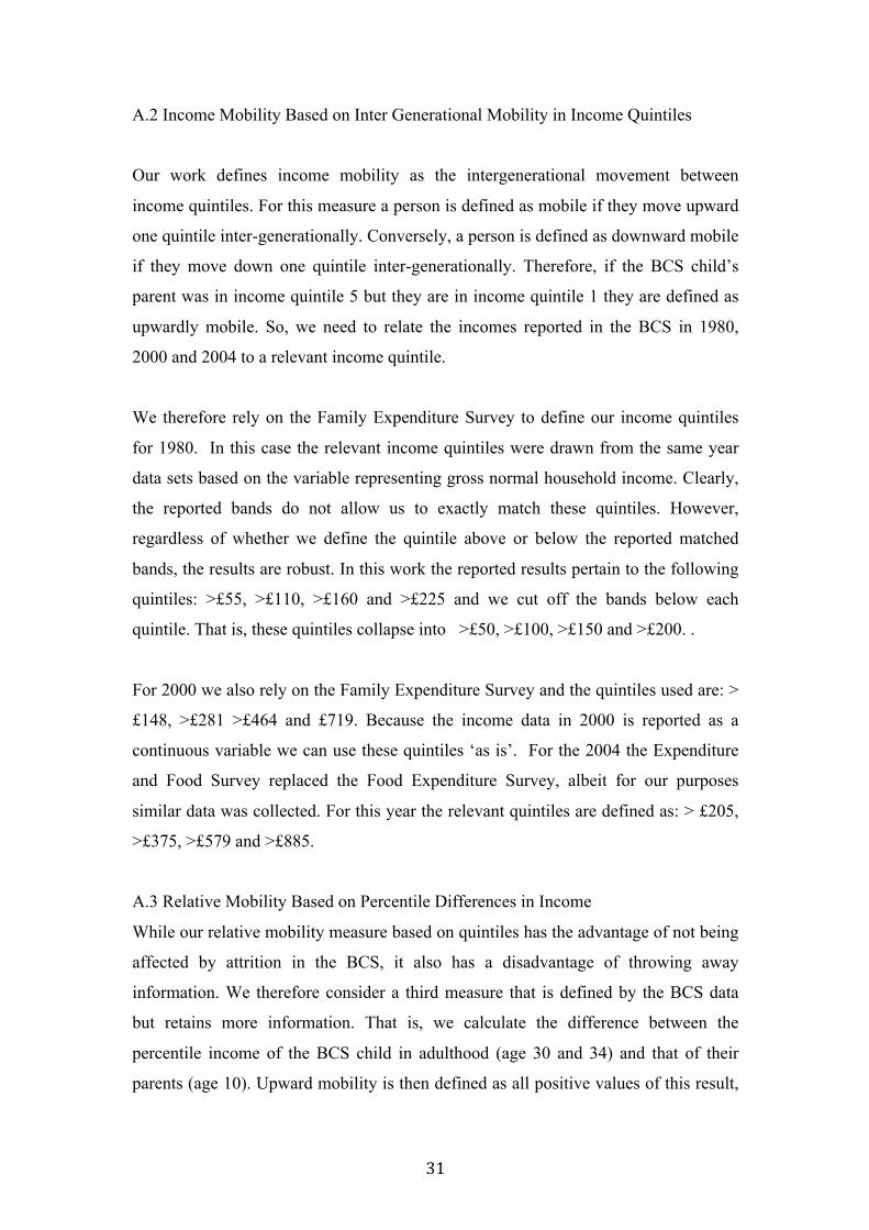
A.2 Income Mobility Based on Inter Generational Mobility in Income Quintiles

Our work defines income mobility as the intergenerational movement between

income quintiles. For this measure a person is defined as mobile if they move upward

one quintile inter-generationally. Conversely, a person is defined as downward mobile

if they move down one quintile inter-generationally. Therefore, if the BCS child’s

parent was in income quintile 5 but they are in income quintile 1 they are defined as

upwardly mobile. So, we need to relate the incomes reported in the BCS in 1980,

2000 and 2004 to a relevant income quintile.

We therefore rely on the Family Expenditure Survey to define our income quintiles

for 1980. In this case the relevant income quintiles were drawn from the same year

data sets based on the variable representing gross normal household income. Clearly,

the reported bands do not allow us to exactly match these quintiles. However,

regardless of whether we define the quintile above or below the reported matched

bands, the results are robust. In this work the reported results pertain to the following

quintiles: >£55, >£110, >£160 and >£225 and we cut off the bands below each

quintile. That is, these quintiles collapse into >£50, >£100, >£150 and >£200. .

For 2000 we also rely on the Family Expenditure Survey and the quintiles used are: >

£148, >£281 >£464 and £719. Because the income data in 2000 is reported as a

continuous variable we can use these quintiles ‘as is’. For the 2004 the Expenditure

and Food Survey replaced the Food Expenditure Survey, albeit for our purposes

similar data was collected. For this year the relevant quintiles are defined as: > £205,

>£375, >£579 and >£885.      

A.3 Relative Mobility Based on Percentile Differences in Income

While our relative mobility measure based on quintiles has the advantage of not being

affected by attrition in the BCS, it also has a disadvantage of throwing away

information. We therefore consider a third measure that is defined by the BCS data

but retains more information. That is, we calculate the difference between the

percentile income of the BCS child in adulthood (age 30 and 34) and that of their

parents (age 10). Upward mobility is then defined as all positive values of this result,

  32  

with negative values recoded to zero. Conversely, downward mobility is then defined

as all negative values of this result, with negative values recoded to zero.

A.4 Absolute Mobility Based on Monetary Differences in Income

In order to create the absolute mobility measure we first transform weekly income

from 1980 and 2000 into 2004 prices. Next, we use 2004 tax rules to form an estimate

of what net take home pay would have been in 1980, based on the weekly gross

earning bands that were collected. Specifically, this translates to

Under £35 per week in 1980 = £56.53 in 2004

£35-£49 per week in 1980 = £127.34 in 2004

£50-£99 per week in 1980 = £199.20 in 2004

£100-£149 per week = £403.81 in 2004

£150-£199 per week =£414.62 in 2004

£200-£249 per week =£530.78 in 2004

£250 or more per week = £626.07 in 2004

We define mobility as weekly net income from adulthood (age 30 or 34 in 2004

prices) minus weekly net income from childhood (age 10 in 2004 prices). As in the

percentile measure, upward mobility is defined as the positive values of this result,

with negative values recoded to zero. Similarly, downward mobility is defined as

negative values of this result, with negative values recoded to zero.

 

CENTRE FOR ECONOMIC PERFORMANCE

Recent Discussion Papers

1189 Nicholas Bloom

Paul Romer

Stephen Terry

John Van Reenen

A Trapped Factors Model of Innovation

1188 Luis Garicano

Claudia Steinwender

Survive Another Day: Does Uncertain

Financing Affect the Composition of

Investment?

1187 Alex Bryson

George MacKerron

Are You Happy While You Work?

1186 Guy Michaels

Ferdinand Rauch

Stephen J. Redding

Task Specialization in U.S. Cities from 1880-

2000

1185 Nicholas Oulton

María Sebastiá-Barriel

Long and Short-Term Effects of the Financial

Crisis on Labour Productivity, Capital and

Output

1184 Xuepeng Liu

Emanuel Ornelas

Free Trade Aggreements and the

Consolidation of Democracy

1183 Marc J. Melitz

Stephen J. Redding

Heterogeneous Firms and Trade

1182 Fabrice Defever

Alejandro Riaño

China’s Pure Exporter Subsidies

1181 Wenya Cheng

John Morrow

Kitjawat Tacharoen

Productivity As If Space Mattered: An

Application to Factor Markets Across China

1180 Yona Rubinstein

Dror Brenner

Pride and Prejudice: Using Ethnic-Sounding

Names and Inter-Ethnic Marriages to Identify

Labor Market Discrimination

1179 Martin Gaynor

Carol Propper

Stephan Seiler

Free to Choose? Reform and Demand

Response in the English National Health

Service

1178 Philippe Aghion

Antoine

Dechezleprêtre

David Hemous

Ralf Martin

John Van Reenen

Carbon Taxes, Path Dependency and Directed

Technical Change: Evidence from the Auto

Industry

1177 Tim Butcher

Richard Dickens

Alan Manning

Minimum Wages and Wage Inequality: Some

Theory and an Application to the UK

1176 Jan-Emmanuel De Neve

Andrew J. Oswald

Estimating the Influence of Life Satisfaction

and Positive Affect on Later Income Using

Sibling Fixed-Effects

1175 Rachel Berner Shalem

Francesca Cornaglia

Jan-Emmanuel De Neve

The Enduring Impact of Childhood on Mental

Health: Evidence Using Instrumented Co-

Twin Data

1174 Monika Mrázová

J. Peter Neary

Selection Effects with Heterogeneous Firms

1173 Nattavudh Powdthavee Resilience to Economic Shocks and the Long

Reach of Childhood Bullying

1172 Gianluca Benigno Huigang

Chen Christopher Otrok

Alessandro Rebucci

Eric R. Young

Optimal Policy for Macro-Financial Stability

1171 Ana Damas de Matos The Careers of Immigrants

1170 Bianca De Paoli

Pawel Zabczyk

Policy Design in a Model with Swings in

Risk Appetite

1169 Mirabelle Muûls Exporters, Importers and Credit Constraints

1168 Thomas Sampson Brain Drain or Brain Gain? Technology

Diffusion and Learning On-the-job

1167 Jérôme Adda Taxes, Cigarette Consumption, and Smoking

Intensity: Reply

1166 Jonathan Wadsworth Musn't Grumble. Immigration, Health and

Health Service Use in the UK and Germany

1165 Nattavudh Powdthavee

James Vernoit

The Transferable Scars: A Longitudinal

Evidence of Psychological Impact of Past

Parental Unemployment on Adolescents in

the United Kingdom

1164 Natalie Chen

Dennis Novy

On the Measurement of Trade Costs: Direct

vs. Indirect Approaches to Quantifying

Standards and Technical Regulations

1163 Jörn-Stephan Pischke

Hannes Schwandt

A Cautionary Note on Using Industry

Affiliation to Predict Income

The Centre for Economic Performance Publications Unit

Tel 020 7955 7673 Fax 020 7404 0612

Email info@cep.lse.ac.uk Web site http://cep.lse.ac.uk