ISSN 2042-2695

CEP Discussion Paper No 1412

March 2016

Relational Knowledge Transfers

Luis Garicano Luis Rayo

Abstract An expert with general knowledge trains a cash-constrained novice. Faster training increases the novice’s productivity and his ability to compensate the expert; it also shrinks the stock of knowledge yet to be transferred, reducing the expert’s ability to retain the novice. The profit-maximizing agreement is a multi-period apprenticeship in which knowledge is transferred gradually over time. The expert adopts a "1/e rule" whereby, at the beginning of the relationship, the novice is trained just enough to produce a fraction 1/e of the efficient output. This rule causes inefficiently lengthy relationships that grow longer the more patient the players. We discuss policy interventions. Keywords: general human capital, international joint ventures, relational contracts JEL codes: IO; LE This paper was produced as part of the Centre’s Growth Programme. The Centre for Economic Performance is financed by the Economic and Social Research Council. We thank Ricardo Alonso, Thomas Bruss, Bob Gibbons, Richard Holden, Hugo Hopenhayn, Larry Samuelson, our discussants Jacques Crémer and Steve Tadelis, seminar participants at the 2013 NBER Working Group in Organizational Economics, the 2015 European Summer Symposium in Economic Theory, and the 2015 CEPR IMO Workshop, and workshop participants at Amsterdam, CEMFI, Chicago, Kellogg, LBS, Milan, and USC for valuable suggestions. Luis Garicano, Department of Management and Department of Economics, London School of Economics and Associate at Centre for Economic Performance, London School of Economics. Luis Rayo, University of Utah and CEPR.

Published by Centre for Economic Performance London School of Economics and Political Science Houghton Street London WC2A 2AE All rights reserved. No part of this publication may be reproduced, stored in a retrieval system or transmitted in any form or by any means without the prior permission in writing of the publisher nor be issued to the public or circulated in any form other than that in which it is published. Requests for permission to reproduce any article or part of the Working Paper should be sent to the editor at the above address. L. Garicano and L. Rayo, submitted 2016.

1 Introduction

As noted by Becker (1994[1964]), training involves a transfer of human capital; thus, un-

like other market transactions, it does not create an asset that can be used as collateral.

Moreover, the novice (apprentice) often does not have the means to pay the expert (mas-

ter), up front, for the knowledge he wishes to acquire. In this case, the rate of knowledge

transfer is constrained by the need to ensure that, over time, the novice has both the

means and the incentives to compensate the expert for his training. Unlike in the first-

best allocation, where knowledge is transferred as fast as technologically feasible, the rate

of knowledge transfer is the result of a trade-off: the faster it is, the sooner output can

be generated; but if it is too fast, the novice will leave without fully compensating the

expert. For example, in professional partnerships, novices, usually called “associates,”

are rewarded for their work not only through their current salary, but also through the

promise of future learning. Such an arrangement allows partners to profit while asso-

ciates are being trained. Similarly, in international joint ventures involving technological

transfers between a “northern”firm (the expert) and a “southern”firm (the novice), the

latter can potentially ignore formal agreements and establish its own operations. As a

result, the rate of knowledge transfer is constrained by the need to ensure a high enough

continuation value for both partners.

The object of this paper is to study, in an environment with limited contractability,

the form and duration of the optimal dynamic relationship between expert and novice.

The goal, in particular, is to explore the speed at which knowledge is transferred, together

with its distributional and effi ciency implications.

We set up a simple model in which an expert and a novice, both of whom are risk-

neutral, interact repeatedly over time. The expert (she) has a stock of general-purpose,

perfectly-divisible knowledge. The novice (he), in contrast, has no knowledge, and there-

fore no ability to produce output; he also has no cash, and therefore no ability to purchase

knowledge from the expert. By transferring knowledge, the expert can raise the novice’s

productivity and, with it, his ability to transfer capital back to the expert. The compli-

cation, however, is that at any time the novice may choose to leave the relationship with

the knowledge already acquired and enjoy the output he is able to produce, on his own,

with this knowledge. Since knowledge is non-contractable and general purpose, the only

repercussion is an end to the players’interactions.

To build a productive relationship in the face of both the novice’s cash constraint and

2

his temptation to walk away from the expert, players rely on a self-enforcing agreement

in which knowledge is transferred gradually over time. Such an agreement is capable

of sustaining knowledge transfers from the expert by providing an expectation of future

payments from the novice; these payments are sustained, in turn, via the expectation of

further knowledge transfers from the expert.

As a benchmark, we first consider relational contracts in which, by assumption, all

knowledge transfers must end after two periods. The optimal arrangement is forward-

looking: the initial knowledge transfer is used as a knowledge “gift”(rather than a loan)

that allows the novice to produce output before the overall knowledge transfer is over;

and the final knowledge transfer is used as an incentive for the novice to surrender such

output. In this two-period arrangement, the expert’s only source of revenue is the output

produced in the first period, using the knowledge gift, which means that the expert is

under pressure to make this gift as large as possible. Because of this pressure, for realistic

values of the players’discount factor, the arrangement is close to first best (and converges

to first best when the discount factor converges to one).

We next turn to the general case in which the expert selects a multi-period arrangement

of any desired length. The optimal contract is an “apprenticeship”arrangement in which,

until the knowledge transfer is complete, players trade labor for training. The structure

of this contract generalizes the two-period arrangement: after an initial knowledge gift,

the novice is asked to work for the expert in exchange for additional knowledge that has a

(discounted) value just high enough to compensate the novice for this work. Equivalently,

this arrangement can be structured as an initial knowledge gift followed by a series of

sales contracts in which, until all knowledge has been sold, the novice devotes 100% of his

output to gradually purchase new knowledge. By delaying consumption until training is

complete, the expert more quickly extract rents from the novice.

The overall length of this apprenticeship is controlled by the size of the initial knowl-

edge gift, with a smaller gift leading to a more distant graduation. When selecting the

optimal gift, the expert faces the following trade-off: a larger gift raises the novice’s

productivity, allowing the expert to extract higher revenues during each period of the ap-

prenticeship; but a larger gift also reduces the amount of knowledge yet to be transferred,

reducing the number of apprenticeship periods that the novice is willing to withstand.

Because of the multi-period nature of the agreement, the expert is in much less of a

rush, relative to the two-period setting, to raise the novice’s productivity early in the

3

relationship.

We find that, no matter how patient players are, and regardless of the details of

the output technology, the optimal knowledge gift allows the novice to produce, at the

beginning of the relationship, a fraction 1eof the effi cient output level (where e is the

mathematical constant). This “1erule”leads to long apprenticeships in which significant

output is wasted. For example, when the annual interest rate is 10% (resp. 5%), training

takes 9.5 years (resp. 19.5 years) to complete. This rule also implies that, in the absence

of other factors affecting the relationship, novices with different skill levels, and novices

working in different professions, take equally long to train.

The optimal apprenticeship is longer, and knowledge is transferred more slowly, the

more patient the players (thus, unlike in the two-period contract, more surplus is wasted

when players are more patient). The reason is that, when patience increases, knowledge

becomes more valuable in the margin (as the novice can use the acquired knowledge during

every subsequent period of his life). Consequently, in any given period the novice is willing

to work for the expert in exchange for a smaller amount of new knowledge; a fact that the

expert exploits by (ineffi ciently) slowing down the training speed and keeping the novice

in her employment for longer.

Motivated by the expert’s preference for artificially lengthy apprenticeships, as well as

by general commentary on real-world masters “exploiting”their apprentices via contracts

with slow training and low consumption (as discussed in Section 2), we consider two policy

experiments. First, we force the expert to pay the novice a minimum wage during training.

We show that while this policy leaves the contract length unaffected (an implication of the

expert’s 1erule), it raises surplus by uniformly accelerating the novice’s’training and, with

it, his output. The reason for this effi ciency gain is that raising the novice’s productivity

allows the expert to partially offset the expense caused by the minimum wage. Second, we

force the expert to contain his interactions with the novice within a shorter horizon. The

result is also an effi ciency gain: the policy alters the expert’s optimal balance between

knowledge gifted and knowledge sold in favor of a larger gift and a faster sale. We end our

policy discussion by illustrating how both of these policies may backfire when the expert

does not enjoy rents to begin with.

Finally, we consider several extensions of the model. First, the case in which the

novice has concave utility, giving him a preference for smooth consumption. In this case,

the expert grants the novice an increasing consumption path that is initially close to

4

zero; representing a compromise between delaying consumption (which allows the expert

to more quickly extract output from the novice) and smoothing consumption (which

helps the novice endure the apprenticeship). Second, we consider brief straightforward

extensions of practical interest: the expert facing training costs, the novice arriving with

capital, and the case in which training causes externalities on the expert (such as an

expert partner in a law firm benefitting when a novice associate becomes a more effective

problem solver, e.g. Garicano 2000, or an expert firm losing profits when training a novice

firm who then becomes a more effective competitor). All of these modifications alter the

optimal contract exclusively via the ratio of knowledge gifted to sold. Finally, we show

that the set of Pareto-effi cient contracts is a family of apprenticeships in which training is

accelerated as the novice’s Pareto weight grows. Taken together, these extensions suggest

that the model’s core results are robust.

The human capital acquisition literature, since Becker’s (1994[1964]) classic analysis,

shows that firms will in principle not pay for general human capital acquisition of their

workers —if they were to do so, they would not recoup their investment, as workers can

always move to another firm. A large literature has aimed to explain, under these circum-

stances, firms’incentives to train their workers by relying on market imperfections. These

imperfections include: imperfect competition for workers (e.g. Stevens, 1994, Acemoglu,

1997, and Acemoglu and Pischke, 1999a,b); asymmetric information about a worker’s

training (e.g. Katz and Ziderman, 1990, Chang and Wang, 1996, and Acemoglu and

Pischke, 1998); and matching frictions (Burdett and Smith, 1996, and Loewenstein and

Spletzer, 1998). In our analysis, in contrast, it is the timing of training, with gradual

training combined with promises of further training down the road, that supports the

knowledge transfer.1

A different literature studies the complementary problem of a firm that, to reward the

investments of its workers in specific human capital, attempts to build credible promises.

Prendergast (1993) argues that, when firms can commit to pay different wages across

tasks, the promise of promotions provides a solution. Relatedly, Kahn and Huberman

(1988) and Waldman (1990) argue that an up-or-out rule leads to credible promises, even

if the promoted worker has similar productivity in all jobs.

1Alternatively, in the learning-by-doing models (following, e.g., Heckman, 1971, Weiss, 1972, Rosen,1972, Killingsworth, 1982, and Shaw, 1989) skill accumulation is a by-product of work. Unlike in thesemodels, our principal has the flexibility to determine the rate at which learning takes place independentlyof the amount of time the agent spends working.

5

Malcomson et al. (2003) study the training of workers using long-term apprenticeship

contracts with an initial period of low wages during which the training firm earns rents,

allowing it to recover its training costs. They study how asymmetric information, con-

cerning both the worker’s intrinsic ability and the firm’s training costs, which are absent

in our model, impact the worker’s training. In their model, all training occurs at the start

of the relationship, before the period of low wages is over.2 (In this setting, workers do not

leave before the low-wage period is over because their ability is not observed by competing

firms.) In our model, in contrast, the timing of training is endogenous, allowing us to

study how knowledge transfers are optimally spread out over time.

Our work is also related to the literature on principal-agent models with relational

contracts, in which, akin to our model, self-enforcing rewards motivate the agent (a few

examples of this growing literature are Bull, 1987, MacLeod and Malcomson, 1989, 1998,

Baker, Gibbons, and Murphy, 1994, Levin, 2003, Rayo, 2007, Halac, 2012, Li and Ma-

touschek, 2013, Barron et al. 2015).3 This literature focuses on eliciting a costly, produc-

tive effort from the agent while treating the agent’s skill level as stationary and exogenous.

In contrast, we treat the agent’s skill as persistent and endogenous while assuming away

effort costs.4

Hörner and Skrzypacz (2010) study a separate challenge underlying knowledge trans-

fers: asymmetric information regarding the value of the knowledge to be sold. They show

that in an environment with limited enforceability, a privately-informed seller benefits

from gradual revelation as a way to provide evidence regarding the quality of her infor-

mation, and therefore raise the price of the information yet to be sold.5 In our model, in

2In this setting, apprenticeships involve a commitment to future wages (which is not possible in ourmodel). The authors show that a regulator can promote training by subsidizing firms and simultaneouslyforcing them to offer contracts with longer periods of low wages after training is over (which is possiblein their setting because of information asymmetries). In our setting, in contrast, a regulator can increasesurplus by forcing firms to limit their knowledge transfers to a shorter training horizon, a considerationabsent in Malcomson et al. (2003). In our setting, since training is gradual, a second policy —a minimumwage during training —may also be beneficial.

3In an alternative setting, Bar-Isaac and Ganuza (2008) study the effect of training on effort in thepresence of career concerns.

4Owing to the liquidity constraint faced by our novice, the “dynamic enforcement” constraint thatgoverns the provision of self-enforcing incentives takes a different form across the two settings: in thecostly-effort setting, this constraint typically indicates that self-enforcing money bonuses cannot exceedthe (stationary) future surplus created by the relationship; in the knowledge-transfer setting, it indicatesthat the money transfers that can be extracted from the novice cannot exceed the (shrinking) value ofthe knowledge yet to be gained by the novice (which represents only a fraction of future surplus).

5Anton and Yao (2002) also consider the sale of information of unknown quality. In their model,to signal quality, the seller reveals part of her information up front. After that, two firms compete to

6

contrast, the value of information is known to all and gradual transmission is instead a

consequence of the buyer being liquidity-constrained —i.e. requiring knowledge to produce

output and compensate the seller with it.

Finally, a related literature studies lender/borrower contracting under limited enforce-

ability (e.g. Thomas and Worrall, 1994, Albuquerque and Hopenhayn, 2004, DeMarzo

and Sannikov, 2006, Biais et al., 2007, and DeMarzo and Fishman, 2007). Limited en-

forceability means that the borrower’s access to capital is restricted; therefore, his output

can grow at most gradually over time. In this lender/borrower setting, transactions in-

volve a single good (capital), whereas in our setting players trade knowledge for capital

(or, equivalently, for labor). As a result, the equilibrium contracts take a different form.

In the lender/borrower setting, absent uncertainty, players write debt contracts in which

debt payments are enforced via the threat of direct punishments on the borrower (i.e.

legal penalties and/or a reduction in the borrower’s access to the productive technology).

In our setting, in contrast, after an initial knowledge gift —rather than a loan —players

engage in a sequence of spot sales contracts, and the reason they remain in the relation-

ship is to benefit from future sales, rather than to avoid punishments.6 As Bulow and

Rogoff (1989) show, in the lender/borrower setting, self-enforcing debt contracts are only

possible when direct punishments are available (otherwise, the agent eventually prefers

to unilaterally reinvest his output rather than using it to honor his debt). In our setting,

with knowledge being noncontractable and general-purpose, such direct punishments are

absent and, yet, are not needed to sustain a productive relationship. Also novel to our

setting is the economic trade-off at the heart of the model: the fraction of knowledge that

the expert sells, rather than gifts, to the novice.

The rest of the paper is organized as follows. Section 2 describes stylized facts in

expert-novice relationships. Sections 3 and 4 present the baseline model and derive the

optimal contracts. Section 5 considers policy experiments and Section 6 considers various

extensions of the baseline model. Section 7 concludes. All proofs are in the Appendix.

purchase the remaining knowledge in a one-shot transaction.6In both cases, provided he is risk-neutral, the agent postpones all consumption until after output has

reached its effi cient level. In the lender-borrower setting, foregoing consumption helps the agent morequickly honor his debt; in our setting, it helps the agent more quickly purchase additional knowledge.

7

2 Some stylized facts

Here we present some empirical observations, concerning knowledge transfers within and

between firms, that serve to motivate our analysis. These observations illustrate the

diffi culties caused by a weak contracting environment and suggest that, often, the resulting

knowledge transfers are ineffi ciently slow.

2.1 Apprenticeships, professional partnerships, and slow knowl-

edge transfers

It has long been observed that apprenticeships may be ineffi ciently lengthy, and training

ineffi ciently slow. According to Adam Smith, “long apprenticeships are altogether un-

necessary... [If they were shorter, the] master, indeed, would be a loser. He would lose

all the wages of the apprentice, which he now saves, for seven years together” (Smith,

1863:56). During the industrial revolution, in extreme cases, training would slow to a

crawl: “[S]ome masters exploited these apprentices’helpless situations, demanding vir-

tual slave labour, providing little in the way of food and clothing, and failing to teach the

novices the trade” (Goloboy, 2008:3). Regarding musical trainees, McVeigh (2006:184)

notes: “Since the master received any earnings from concert appearances, apprentices were

inevitably subject to exploitation [. . . ] Other apprentices he set to menial tasks. Burney

[the apprentice] recorded with irritation the drudgery he undertook for Arne [the master]

in the mid 1740s: Music copying, coaching singers and so on.”

Similar observations are often made of present-day training relationships. According

to a UK government inquiry: “Several apprentices reported that they were being used as

cheap labour [...] Typical responses from apprentices were that [...] they were used to

do menial tasks around the workplace”(Department for Business, Innovation and Skills,

2013).7

An important instance of knowledge transfers occurs in professional service firms.

These firms provide a wide range of general skills to junior consultants, usually called

associates (see, for example, Maister, 1993, and Richter et al., 2008). Once again, training

appears to be slowed down, artificially, while associates “pay their dues.”In the process,

7“Apprentices’ Pay, Training and Working Hours.” BIS, UK Government, 2013.(https://www.gov.uk/government/uploads/system/uploads/attachment_data/file/49987/bis-13-532-follow-up-research-apprentices-pay-training-and-working-hours.pdf.)

8

rents are extracted from their work in exchange for the promise of further training and

eventual promotion.8

At law firms, for example, the training of associates seems, anecdotally, to proceed at

a glacial pace; as a result, associates are forced into menial tasks. Numerous blog posts

and articles are dedicated to describing this feature. For instance, according to a former

litigator, “this recession may be the thing that delivers them from more 3,000-hour years

of such drudgery as changing the dates on securitization documents and shuffl ing them

from one side of the desk to the other”... “it often takes a forced exit to break the leash

of inertia that collars so many smart law graduates to mind-numbing work”(New York

Times, 2009).9 Similarly, as an Australian Justice observes, “young solicitors are being

exploited and overworked by law firms that have lost sight of their traditional duty to

nurture the next generation of lawyers.”10 Perhaps not surprisingly, the response of the

American Bar Association (ABA) is to tough it out. The ABA admonishes, in its advice

to young lawyers: “No task is too menial that you can’t learn from it.”11

2.2 International joint ventures and limited contractability

International joint ventures between a “northern”firm in a developed country (the ex-

pert) and a “southern” firm in a developing country (the novice) frequently involve a

technology transfer in exchange for a cash flow. Often, owing to weak institutions in the

developing country, the partners cannot rely on legally-enforced contracts; as a result,

their relationship becomes analogous to one in which knowledge is transferred between

two individuals. In this case, the relationship only lasts for as long as the parties consider

it in their common interest to continue their “knowledge-for-cash”exchange.

A notable example is the failed partnership of Danone and Wahaha. Their relation-

ship began in 1996 when Danone, a French drink and yogurt producer, established a joint

venture with the Hangzhou Wahaha group, a Chinese producer of milk drinks for chil-

dren. (See, for example, Financial Times, April 2007.)12 For Danone, the venture was

a way to profit from the growing Chinese market; for Wahaha, it was a means to learn

8Levin and Tadelis (2005) provide an alternative view of partnerships. There, partnerships serve as acommitment device to provide high-quality service in a context of imperfect observability.

9“Another View: In Praise of Law Firm Layoffs.”NYT. Dealbook. July 1, 2009. By Dan Slater.10http://www.theaustralian.com.au/business/legal-affairs/firms-exploiting-young-lawyers-says-chief-

justice-marilyn-warren/story-e6frg97x-1226717910085.11http://apps.americanbar.org/litigation/committees/trialpractice/younglawyers.html.12“How Danone’s China venture turned sour.”FT. April 11, 2007. By Geoff Dyer.

9

Danone’s technology. Initially, the joint venture was highly successful, contributing 5-

6% of Danone’s entire operating profits. However, in 2007, after Wahaha learned what it

needed, it set up a parallel organization that served its clients outside of the joint venture.

Danone appeared, legally, to have the upper hand, as it owned 51% of the joint

venture. However, its power was not real. As noted by the press, “the joint venture

depends on Mr. Zong’s [Wahaha’s boss] continuing cooperation. Not only is he chairman

and general manager of the joint venture, but he is the driving force behind the entire

Wahaha organization. Furthermore, in China, employees in private enterprises often feel a

stronger loyalty to the boss than the organization itself. Winning in the courts or pushing

out Mr. Zong, therefore, are not solutions to Danone’s problems.”(Financial Times, April

2007). Workers were strongly behind Zong: “We formally warn Danone and the traitors

they hire, we will punish your sins. We only want Chairman Zong. Please get out of

Wahaha!”(Financial Times, June 2007).13 In the end, Danone lost all its court battles

in China, and with them its trademarks.

The Danone-Wahaha case is far from unique; indeed, anecdotal evidence suggests

that these types of disputes are quite common. For example, in a case involving two

industrial machinery manufacturers, Ingersoll-Rand claimed that Liyang Zhengchang had

breached their joint-venture agreement by manufacturing and selling imitation processing

equipment based on Ingersoll-Rand’s patents.14 Once again, the Chinese authorities sided

with the Chinese partner.

In the previous examples, the northern partner appears to have underestimated the

weakness of the legal institutions in question; as a result, it failed to appreciate the

dynamic inconsistency of the exchange. A case in which the northern partner seems fully

aware of such challenges is the auto-manufacturing alliance between General Motors (GM)

and the Chinese manufacturer SAIC. As GM’s chairman points out: “We have a good

and viable relationship and partnership. But to make it work, you have to have needs

on both sides of the table” (Wall Street Journal, 2012).15 GM was careful to provide

enough knowledge to make the relationship valuable for SAIC: “SAIC [...] went into the

partnership with big dreams but little know-how. Today the companies operate much

more like equals.”At the same time, presumably mindful of the self-enforcing nature of

13“Still waters run deep in dispute at Wahaha.”FT. June 12, 2007. By Geoff Dyer.142000 U.S. Dist. LEXIS 18449.15“Balancing the Give and Take in GM’s Chinese Partnership.”WSJ. August 19, 2012. By Sharon

Terlep.

10

the relationship, GM has not yet transferred some of its most valuable knowledge: “GM

is holding tight to its more valuable technology. Beijing is eager to tap into foreign auto

companies’clean-energy technologies. But GM doesn’t want to share all its research with

its Chinese partner”. Indeed, “SAIC could use GM expertise and technology to transform

itself into a global auto powerhouse that challenges the American car maker down the

road.”

3 Baseline model

There are two risk-neutral players: an expert E (she) and a noviceN (he). Players interact

over infinite periods t = 1, 2, ... and discount future payoffs using a common interest rate

r > 0. Let δ = 11+r

denote the players’discount factor. The expert possesses one unit

of general-purpose knowledge. This knowledge is perfectly divisible, does not depreciate,

and can be transferred from the expert to the novice at any speed desired by the expert.

Let xt ∈ [0, 1] denote the fraction of knowledge transferred during period t and let Xt

denote the novice’s total knowledge, inclusive of xt, during period t:

Xt = xt +Xt−1,

with X0 = 0.

During period t, the novice produces output f(Xt) ∈ R+, with f continuous and

increasing, and f(0) = 0. One interpretation is that the novice’s output originates from

a variety of tasks, with less valuable tasks requiring less knowledge. In this case, as the

novice acquires knowledge, he effi ciently spends less time on menial tasks and more on

advanced ones.16 For the time being, to highlight the expert’s desire for an artificially slow

knowledge transfer, we assume that the expert faces no costs when training the novice.17

Let P (X ′, X) = 11−δ [f(X ′)− f(X)] denote the marginal value of a package of knowledge

containing X ′ −X units, in present discounted terms, starting from an initial knowledge

stock X.16For example, a cook may either engage in the menial task of chopping vegetables or in the advanced

task of making sauces (e.g. Gergaud et al., 2014). Similarly, a consultant may either perform lengthyspreadsheet calculations or simply advise others on what objects to calculate (e.g. Garicano, 2000). Ineither case, only after appropriate training is the worker successful at the advanced task.17This assumption rules out both direct training costs and externalities experienced by the expert as

the novice becomes more knowledgeable. In Section 6.2, we extend the model to illustrate the impact ofsuch costs.

11

The novice has a bank account that pays interest r between periods. Let (1 + r)Bt−1

and Bt denote, respectively, the balance of this account at the beginning and end of period

t. The novice cannot borrow from his bank (Bt ≥ 0) and, for now, has no initial capital

(B0 = 0). The expert, in contrast, has deep pockets.

Each period t has three stages. First, there is a knowledge-transfer stage in which

players swap knowledge for cash: the expert makes a knowledge transfer xt and the novice

makes a money transfer mt ∈ R in return. Players rely on a spot contract for this swap.Each player i = E,N simultaneously proposes a pair (xit,m

it) subject to two feasibility

constraints: (1) xit is no larger than the expert’s remaining knowledge stock 1−Xt−1; (2)

mit is no larger than the novice’s current savings (1 + r)Bt−1. If (xEt ,m

Et ) = (xNt ,m

Nt ) an

agreement is reached and the corresponding transfers take place: xt = xEt and mt = mEt .

Otherwise, no agreement is reached and xt = mt = 0.

Second, there is a production stage in which the novice either works on her own (dt = 0)

or works for the expert (dt = 1), and the expert pays a wage wt ∈ R to the novice.

Players rely on a spot employment contract. Each player simultaneously proposes a pair

(dit, wit) (with d

it ∈ 0, 1) subject to −wit not exceeding the novice’s current bank balance

(−wit ≤ (1 + r)Bt−1 − mt). If (dEt , wEt ) = (dNt , w

Nt ) an agreement is reached: dt = dEt

and wt = wEt . Otherwise, dt = wt = 0. Since knowledge is general, output f(Xt) is

independent of the employment decision.

Third, there is a consumption stage in which the novice splits his stage-2 earnings

wt+(1− dt) f(Xt) and remaining balance (1+r)Bt−1−mt between consumption ct ∈ R+

and savings. His resulting end-of-period balance is

Bt = wt + (1− dt) f(Xt) + (1 + r)Bt−1 −mt − ct.

All variables are observed by both players. In addition, the only formal (court-

enforced) contracts that can be written are the one-period spot contracts described above.

All other agreements must be self-enforced.18

From the standpoint of the beginning of period t, the continuation payoffs for expert

18If the expert had commitment power (e.g. owing to external reputation concerns), the assumptionthat spot contracts are court-enforced would not be required.

12

and novice are, respectively,

Πt =∞∑τ=t

δτ−t [mτ + dτf(Xτ )− wτ ] and

Vt =

∞∑τ=t

δτ−tcτ = (1 + r)Bt−1 +

∞∑τ=t

δτ−t [−mτ + (1− dτ ) f(Xτ ) + wτ ] .

Since the players’combined surplus is Π1 +V1 =∑∞

t=1 δt−1f(Xt), the first-best allocation

calls for a full knowledge transfer in the first period.

A self-enforcing relational contract (or more briefly, a contract) prescribes, on the path

of play, a vector 〈Xt,mt, dt, wt, ct〉 for every period t; and, upon any deviation from that

prescription, it prescribes a suspension of all further transactions between the players.19

For notational simplicity we denote a contract by its prescribed actions on the path of

play: C = 〈Xt,mt, dt, wt, ct〉∞t=1. Let Πt(C), Vt(C), and Bt(C) denote, respectively, theequilibrium values of Πt, Vt, and Bt. Also let Ω denote the set of contracts C that satisfythe basic requirements that xt ≤ 1−Xt−1, Bt(C) ≤ 0, and ct ≥ 0 for all t. We say that a

contract C is feasible if it belongs to Ω and, in addition, it constitutes a subgame-perfect

equilibrium of the dynamic game.

Feasibility of C requires that six constraints are met for every period t—three con-straints for each of the first two stages.20 As we show momentarily, however, all stage-2

constraints are redundant.

Stage-1 constraints

From the standpoint of the beginning of stage 1, both players must weakly prefer to

follow their prescribed actions over reneging on the agreement:

Πt(C) ≥ 0 for all t, (1)

Vt(C) ≥1

1− δ f(Xt−1)︸ ︷︷ ︸value of knowledge

+ (1 + r)Bt−1(C)︸ ︷︷ ︸current balance

for all t. (2)

19These trigger punishments are in principle not immune to renegotiation. As we shall see, however,the optimal relational contract is itself immune to renegotiation.20In principle we may also require a constraint for stage 3, in which the novice makes his consump-

tion/savings decision. This constraint, however, is redundant because, because being risk-neutral andearning interest r, the novice can always replicate an “over-consumption”deviation in this stage with adeviation in stage 1 of the following period in which he walks away with his savings.

13

The novice’s constraints require that he weakly prefers his continuation payoff over walk-

ing away with his current stock of knowledge Xt−1 (worth 11−δf(Xt−1) in present value)

together with his current cash balance. We call these two constraints the players’incentive

constraints.

In addition, the novice must have suffi cient liquidity to afford the transfers mt:

mt ≤ (1 + r)Bt−1(C) for all t. (3)

Stage-2 constraints

From the standpoint of the beginning of stage 2, both players must again be deterred

from reneging on the agreement:

dtf(Xt)− wt︸ ︷︷ ︸stage-2 revenues

+ δΠt+1(C) ≥ 0 for all t, (4)

Vt(C) ≥1

1− δf(Xt−1)︸ ︷︷ ︸value of knowledge

+ (1 + r)Bt−1(C)−mt︸ ︷︷ ︸current balance

for all t. (5)

The novice must also be able to afford the transfers −wt:

−wt ≤ (1 + r)Bt−1(C)−mt for all t. (6)

Lemma 1 tells us that, without loss, the residual claim of output can be granted to the

novice and wages can be set to zero. As a result, all stage-2 constraints are redundant:

Lemma 1 Let C = 〈Xt,mt, dt, wt, ct〉∞t=1 be a feasible contract. There exists a feasible

contract C ′ = 〈Xt,m′t, d′t, w

′t, ct〉

∞t=1 that prescribes the same knowledge transfers and equi-

librium payoffs Π1, V1 as contract C and under which, in every period, the novice is theresidual claimant of output (d′t = 0) and receives zero wages (w′t = 0). Moreover, under

contract C ′ all stage-2 constraints ((4), (5), and (6)) are redundant.

Intuitively, since knowledge is general, it is immaterial whether the residual claimant

of output is the novice or the expert. In the former case, the novice’s most tempting

deviation consists in walking away from the relationship during the knowledge-transfer

phase of a given period t, before making any money transfer to the expert. In the latter

14

case, the novice’s most tempting deviation is identical except for the fact that it is initiated

during the production phase of period t−1, with the novice producing output f(Xt−1) on

his own rather than for the expert. In present-discounted terms, both deviations deliver

the same payoff.

In what follows, we set dt = wt = 0 for all t and refer to a relational contract simply

as C = 〈Xt,mt, ct〉∞t=1 . We define a “training period”of C as a period in which the novicereceives knowledge (xt > 0) and the “training phase”of C as the set of all its trainingperiods. We also let Xsup(C) = limt→∞Xt denote the total knowledge transferred under

C.

4 Optimal contracts

An optimal contract solves the expert’s profit-maximization problem:

maxC∈Ω

Π1(C) (I)

s.t. (1), (2), and (3).

To build intuition, we begin with a simple benchmark in which, by assumption, all

transactions end after two periods. We then turn to contracts of optimal length. Through-

out, to avoid knife-edge cases in which there is more than one solution, we assume δ is

“generic”in the sense that 11−δ 6= n for all n ∈ N.

4.1 Benchmark: two-period contracts

Here we consider contracts in which, by assumption, knowledge and money transfers are

restricted to occur in the first two periods of the game (i.e. xt = mt = 0 for all t > 2).

The expert’s problem is

maxC∈Ω

m1 + δm2

s.t. m1 ≤ 0,

m2 ≤ min

P (X2, X1)︸ ︷︷ ︸Value of X2−X1

, (1 + r)B1(C)︸ ︷︷ ︸Available cash

, (IC + L)

15

Constraint (IC+L) tells us that m2 must be weakly below both the marginal value of the

knowledge transferred in the second period and the novice’s cash balance at beginning of

that period. A higher initial knowledge level X1 increases the novice’s subsequent liquidly,

but also reduces his willingness to pay for the remaining knowledge X2 −X1, as there is

less of it. (In this two-period benchmark, the expert’s own incentive constraints (1) are

redundant.) The optimal contract belongs to a simple class:21

Remark 1 Any optimal two-period contract C = (Xt,mt, ct)t=1,2 consists of a knowledge

gift X1 > 0 and a money loan m1 ≤ 0 in period 1 followed by a spot contract in period

2 in which the novice devotes the full balance of his bank account to purchase additional

knowledge X2 −X1 > 0 at a price equal to marginal value P (X2, X1). Namely,

m2 = (1 + r)B1(C) = P (X2, X1).

When selecting the total knowledge transferX2 and the first-period consumption level,

the expert’s only goal is to maximize the magnitude of the second-period knowledge sale.

For this reason, she opts for a full knowledge transfer (which maximizes the amount of

knowledge that is sold) and zero first-period consumption (which maximizes the novice’s

purchasing power).

The initial knowledge gift and money loan must now solve:

maxX1>0,m1≤0

m1 + δP (1, X1)

s.t. P (1, X1) = (1 + r) [f(X1)−m1] .

We learn that offering a loan is counterproductive: while it increases the novice’s purchas-

ing power during the subsequent knowledge sale, it can only be recovered if the expert

simultaneously increases the price P (1, X1) by shrinking X1, which in turn hurts the

expert as the first-period output is her only net source of revenues.

Finally, the optimal knowledge gift, obtained by setting P (1, X1) = (1 + r)f(X1),

satisfiesf(X1)

f(1)= δ.

21An equivalent interpretation is that the principal sells X1 at an arbitrary price p > 0 to be paid inperiod 2. Then, in period 2, the principal collects p and simultaneously sells X2 − X1 at a discountedprice P (X2, X1)−p. Such arrangement, however, is economically identical to that described in the remark(in which p = 0).

16

This gift is increasing in δ and approaches 100% of knowledge as δ approaches 1. The

reason is that as players become more patient, the present value of any incremental knowl-

edge grows without bound, which in turn allows the expert to extract all of the novice’s

first-period output in exchange for an ever smaller second-period knowledge transfer. Note

also that the arrangement creates a deadweight loss equal to f(1)− f(X1) = (1− δ)f(1).

As δ approaches 1, this loss vanishes.

As we shall see next, once the expert is free to select the overall length of the contract,

allowing her to capture output produced over multiple periods, she is in much less of a

rush to increase the novice’s productivity. As a result, she opts for lengthy contracts in

which the above comparative statics are overturned.

4.2 Optimal contracts of unrestricted length

Here we return to the general setting in which contracts are allowed to have an arbitrary

length. This setting allows for a rich set of contracts in which the expert may spread

knowledge gifts and sales over arbitrarily many periods and may also use monetary rewards

to keep the novice in the relationship. We begin by focusing on the relaxed problem in

which the expert’s incentive constraints are ignored:

maxC∈Ω

Π1(C) = maxC∈Ω

∞∑t=1

δt−1mt (II)

s.t. (2) and (3).

Lemma 2 rules out contracts of infinite length in which training is carried out over

infinitely many periods:

Lemma 2 Every contract C that solves the expert’s relaxed problem (II) has a finite

training phase, namely, Xt = Xsup(C) for some t.

Intuition is as follows. Consider a contract of infinite length. From the standpoint of

any given date, the total (discounted) transfer that the expert can hope to extract from

the novice is no greater than the value of the knowledge yet to be transferred. Moreover,

since knowledge is finite, this value must necessarily approach zero as time goes by. As a

result, the expert can instead end the contract early by selling all remaining knowledge

at once, which the novice can eventually afford, and benefit from earlier revenues.

17

We now define a class of contracts, which we call “delayed-reward”contracts, and note

that the expert can restrict attention to this class.22

Definition 1 A finite contract C is a delayed-reward contract if it requires that 100%of output produced before a given period T is transferred to the expert and, in return,

the expert grants the novice a one-time cash bonus M during period T , after which all

transactions end and the novice keeps 100% of output. The net money transfers under

such contract satisfy:

m1 = 0, mt = (1 + r) f (Xt−1) for t ∈ 2, ..., T − 1 , and mT = (1 + r) f (XT−1)−M.

In such arrangements, the novice is willing to endure the training phase, during which

he receives zero output, in exchange for both additional training and the eventual cash

bonus M. Since in the present baseline model the novice cares only about his total (dis-

counted) consumption and not its timing, these arrangements are effi cient and also max-

imize the novice’s incentives to remain in the relationship.

Remark 2 Let C ∈ Ω be a finite contract that satisfies constraints (2) and (3). There

exists a delayed-reward contract C ′ ∈ Ω that satisfies both constraints and delivers the

same equilibrium payoffs Π1, V1 as contract C.

In a delayed-reward contract, the novice’s incentive constraint for period t < T takes

the following form:

(1 + r)T−1∑τ=t

δτ−tf(Xτ )︸ ︷︷ ︸Output surrendered to the expert

≤T−1∑τ=t

δτ−tP (Xτ+1, Xτ ) + δT−tM︸ ︷︷ ︸Future knowledge and bonus rewards

, (7)

which captures the fact that, knowledge being general, the novice is only willing to work

for the expert in exchange for future knowledge and money transfers, not for past ones.

In present discounted terms, the L.H.S. is the output the novice is asked to surrender

during the remaining periods of training and the R.H.S. is the benefit the novice receives

22An economically equivalent arrangement is one in which the bonus M is paid over multiple periodst ≥ T (while keeping its present discounted value constant) rather than being concentrated on period Talone. We also refer to such an arrangement as a delayed reward contract.

18

in return, namely, the value of the knowledge XT − Xt he is yet to acquire, plus the

bonus.23

This constraint places an upper bound on the knowledge that the novice can be trusted

with at any point during training: a higher Xt means that the novice is asked to surrender

more output during training and, simultaneously, it lowers the value of the additional

knowledge he is offered as compensation. It also shows that the expert can increase Xt,

and therefore the novice’s productivity, in three ways: a larger total knowledge transfer

XT , a larger bonus, and an earlier graduation date.

Lemma 3 shows that every optimal delayed-reward contract prescribes a suffi ciently

fast knowledge transfer so that, in any given period, the novice is able to produce no less

than the incremental value of the knowledge he acquires (in other words, the expert keeps

only the minimal amount of knowledge needed to prevent the novice from leaving):

Lemma 3 Suppose a delayed-reward contract C (prescribing a one-time bonus M during

period T ) solves problem (II). Then, C has the property that, in every period t > 1, the

novice pays a gross price no lower than the marginal value of the knowledge he acquires:

mt +M · 1t=T ≥ P (Xt, Xt−1). (8)

This result tells us that the novice gains surplus, at most, at the very beginning of

the relationship (through a knowledge gift) and at the very end (through the bonus). In

every other period, the novice surrenders all his output in exchange for knowledge that

he values in no more than this output. Intuitively, if the expert is to gift any amount of

knowledge (for instance, by selling a fraction of knowledge at a price lower than marginal

value), it is most effi cient to concentrate this gift at the beginning of the relationship as

it allows the novice to raise his productivity sooner; and if the expert is to offer a money

bonus, for incentive reasons it is best to defer this bonus until all other transactions are

over. Note also that, when the novice is expecting a bonus, he may be willing to pay a

price larger than P (Xt, Xt−1) for the right to remain in the relationship.

23In the parlance of relational contracts, this incentive constraint represents a “dynamic enforcement”constraint that indicates the extent to which future surplus can be recruited to enforce current moneytransfers from the novice. In the present setting, only a fraction of future surplus (the fraction pocketedby the novice) can be used for this purpose. In contrast, in the standard principal-agent setting, inwhich both players have deep pockets and therefore surplus can be freely redistributed across them (e.g.Levin, 2003), the players’entire continuation surplus can be recruited to enforce money transfers in anydirection.

19

We now return to the expert’s original problem. Proposition 1 shows that the bonus

can be dispensed with and describes the overall structure of an optimal contract:

Proposition 1 In the baseline model, every optimal contract — solving problem (I) —

consists of a knowledge gift in period 1 followed by a sequence of spot sales contracts in

which the novice devotes all period t output (plus interest) to purchase knowledge Xt+1−Xt

in period t+1 at a price equal to marginal value P (Xt+1, Xt). This process continues until

100% of knowledge has been transferred, after which all transactions end.

An optimal contract is equivalent to an “apprenticeship”(work-for-training) arrange-

ment in which, until the knowledge transfer is complete, the novice works for the expert

and is compensated exclusively through additional knowledge. Specifically, during each

period before the knowledge transfer is complete, the novice is asked to produce output

f(Xt) for the expert, rather than for himself; in return, at the beginning of the following

period, the novice is granted a package of knowledge [Xt, Xt+1] that has a (discounted)

value δ1−δP (Xt+1, Xt) just high enough to offset this output loss. The overall length of

this apprenticeship is controlled by the size of the initial knowledge gift, with a smaller

gift leading to a more distant graduation.

Intuition for Proposition 1 is as follows. First, recall that for a given total knowledge

transfer, the expert has two instruments for raising the novice’s productivity during train-

ing: a bonus and an earlier graduation date. Of the two, the bonus is a finer instrument

as, unlike an earlier graduation date, it allows the expert to raise output continuously.

However, since the incentive constraints (7) are linear in both output and the bonus,

whenever a bonus is used the expert adopts a “corner” solution in which the bonus is

raised to the point that output hits its upper bound f(1) during some period before the

contract is over. This large bonus can then be replaced, without loss, by a shorter con-

tract with the same output path but that allows the novice to graduate as soon as output

reaches f(1).24 Second, the price of knowledge is derived from Lemma 3: on the one hand,

any knowledge sold at a price lower than marginal value amounts to a fraction of knowl-

edge being gifted, but the novice’s productivity can be raised by speeding up all such

24The optimal output path can also be implemented with bonuses of varying size. Every such imple-mentation calls for a bonus that is a multiple of the effi cient output f(1) (plus appropriate interest),which results in the expert retaining the novice for a number of periods after the knowledge transferis complete. All such implementations, however, call for a net transfer of cash from the expert in thelast period of interaction, which is not feasible once the expert’s participation constraints are imposed.Uniqueness of the optimal arrangement follows from this fact.

20

gifts and concentrating them in the first period of the relationship, before the knowledge

sale begins; on the other hand, once the bonus is set to zero, and given that the price

of knowledge never falls below marginal value, in no period is the novice willing to pay

more than marginal value. Finally, given that the expert captures all surplus during the

knowledge sale, she finds it optimal to sell all of her knowledge.

Before we further characterize the optimal contract, some remarks are in order:

• When selecting the optimal length of the apprenticeship, the expert faces the fol-lowing trade-off: by raising the novice’s productivity, a larger knowledge gift allows

the expert to extract higher revenues during each training period; but since it also

reduces the amount of knowledge left for sale, it reduces the number of training

periods that the novice is willing to withstand. As we shall see, this trade-off,

which is central to the remainder of the paper, results in lengthy contracts in which

significant output is wasted.

• The above apprenticeship calls for an extreme form of training in which the novice

is forced to consume zero until training is complete, at which point he graduates and

his consumption experiences a sudden increase. Below, we also consider less extreme

arrangements in which, owing to either government intervention or the novice being

risk averse, consumption is positive (though still low) during training.

• We have assumed that any deviation from a contract’s prescriptions is punished

through permanent separation. Since separation typically results in a destruction

of output, it need not be immune to renegotiation. Fortunately, because of its

forward-looking nature, the above apprenticeship can be recast to avoid this pitfall,

as follows. After receiving the knowledge gift, the novice is invited, every period,

to purchase any amount of knowledge he desires at a price equal to the marginal

value P of the knowledge he wishes to acquire. Even if, in a given period, the

expert deviates by not selling knowledge under these terms, or the novice deviates

by failing to make such a purchase (or by devoting only part of his output to the

purchase), the players remain invited to meet again the following period, under the

same terms as before.

21

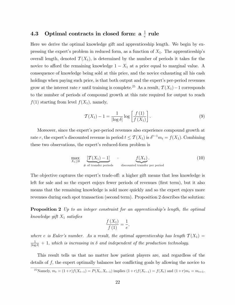
4.3 Optimal contracts in closed form: a 1e rule

Here we derive the optimal knowledge gift and apprenticeship length. We begin by ex-

pressing the expert’s problem in reduced form, as a function of X1. The apprenticeship’s

overall length, denoted T (X1), is determined by the number of periods it takes for the

novice to afford the remaining knowledge 1 − X1 at a price equal to marginal value. A

consequence of knowledge being sold at this price, and the novice exhausting all his cash

holdings when paying such price, is that both output and the expert’s per-period revenues

grow at the interest rate r until training is complete.25 As a result, T (X1)−1 corresponds

to the number of periods of compound growth at this rate required for output to reach

f(1) starting from level f(X1), namely,

T (X1)− 1 =1

|log δ| log

[f (1)

f (X1)

]. (9)

Moreover, since the expert’s per-period revenues also experience compound growth at

rate r, the expert’s discounted revenue in period t ≤ T (X1) is δt−1mt = f(X1). Combining

these two observations, the expert’s reduced-form problem is

maxX1≥0

[T (X1)− 1]︸ ︷︷ ︸# of transfer periods

· f(X1)︸ ︷︷ ︸ .discounted transfer per period

(10)

The objective captures the expert’s trade-off: a higher gift means that less knowledge is

left for sale and so the expert enjoys fewer periods of revenues (first term), but it also

means that the remaining knowledge is sold more quickly and so the expert enjoys more

revenues during each spot transaction (second term). Proposition 2 describes the solution:

Proposition 2 Up to an integer constraint for an apprenticeship’s length, the optimal

knowledge gift X1 satisfiesf (X1)

f (1)=

1

e,

where e is Euler’s number. As a result, the optimal apprenticeship has length T (X1) =1|log δ| + 1, which is increasing in δ and independent of the production technology.

This result tells us that no matter how patient players are, and regardless of the

details of f, the expert optimally balances her conflicting goals by allowing the novice to

25Namely, mt = (1 + r)f(Xt−1) = P (Xt, Xt−1) implies (1 + r)f(Xt−1) = f(Xt) and (1 + r)mt = mt+1.

22

produce, at the start of the apprenticeship, a share 1eof the effi cient output level. Indeed,

upon combining (9) and (10), the expert’s problem is equivalent to that of maximizing

the average logarithm log[f(1)f(X1)

]·[f(1)f(X1)

]−1

of the output ratio f(1)f(X1)

. The maximum is

achieved when this ratio is e.When each period consumes an arbitrarily small amount of

time (as formalized in Section 4.3.B below), this solution also has the property of equating

the present value of knowledge gifted (1eP (1, 0)) to the present value of knowledge sold

(∑T (X1)

t=2 δt−1P (Xt, Xt−1)). As a result, surplus is split 50-50 between the two players.

The present solution coincides with the solution to the “secretary problem”in which

a recruiter who faces a queue of job applicants of unknown quality must decide what

fraction of applicants to sample before making any hiring decision (e.g. Bruss, 1984).

As the total number of applicants tends to infinity, the optimal sample converges to a

fraction 1eof all applicants (a result sometimes called a “1

elaw”). While the two problems

have the same solution, they do not appear to have any direct economic link. In addition,

unlike in the secretary problem, we obtain a 1erule for transactions of finite duration.26

Notice that the optimal apprenticeship is longer, and knowledge is transferred more

slowly, the more patient the players. Intuitively, when the interest rate r falls, knowledge

becomes more valuable, in the margin, to the novice (as he can use this knowledge during

every subsequent period of his life). As a result, a lower interest rate means that, each

period, the novice is willing to work for the expert in exchange for a smaller amount of new

knowledge. The expert takes advantage of this fact by stretching out the training phase

and keeping the novice with her longer. (Notice also the contrast with the two-period

contract derived in Section 4.1. There, the knowledge gift grows as r falls, and converges

to 100% of knowledge as r converges to 0.)

Consistent with real-world practices noted in Section 2, the expert’s 1erule causes

lengthy apprenticeships. For instance, training takes approximately 9.5 years when the

annual interest rate is 10% and approximately 19.5 years when the interest rate is 5%.

This rule also means that the details of f do not affect the length of the apprenticeship.

The implication is that, in the absence of other factors affecting the relationship, novices

of different skill levels, and novices working on different tasks, take equally long to train.

Before turning to policy implications, we discuss the ineffi ciencies caused by these long

training phases and well as the impact of increasing the players’frequency of interaction

(while holding constant their underlying discount rate):

26We are grateful to Thomas Bruss for providing insights on the secretary problem.

23

A. Effi ciency and the role of δ

Here we consider the deadweight loss associated to the optimal contract. Recall that

the contract is socially ineffi cient as it artificially spreads the knowledge transfer over

multiple periods. The resulting loss in surplus (namely, the present value of the loss in

output relative to first best) is

|log δ|−1∑t=1

[δt−1 − 1

e

]f(1).

This loss increases with δ for two reasons. First, a higher δ leads to a longer training phase

and, with it, a slower knowledge transfer. Second, a higher δ implies that the ineffi ciencies

caused by the slower transfer loom larger from the perspective of period 1.

When measured as a fraction of first-best surplus, P (1, 0), the loss is 1 − 1e− 1−δ|ln δ|

1e. In

contrast to the absolute loss, this relative loss falls with δ because first-best surplus grows

with δ faster than the deadweight loss. However, as δ converges to 1 this loss remains

bounded away from zero: it is no smaller than e−2e' 25% of first-best surplus.

B. Frequency of interaction

Here we ask whether allowing players to interact with higher frequency (multiple times

during each date t) alters the length of the optimal apprenticeship, measured in calendar

time. One may wonder, for instance, if the apprenticeship consumes an arbitrary short

amount of time when players are allowed to interact arbitrarily often.27 We show that,

modulo the time it takes to exchange the initial knowledge gift (which is the length of time

consumed by stage 1 in a given period), the overall time consumed by the apprenticeship

is invariant in the frequency of interaction.

We assume that date t consumes one year and consists of n ≥ 1 periods. Accordingly,

δ is the annual discount factor and δ1/n the per-period factor. Denote a period by τ and

let per-period output be f(Xτ , n), with f1 > 0, f2 < 0, and limn→∞ n · f(1, n) < ∞.28 Agiven period τ within date t consumes 1

nyears. Note that this setting is equivalent to the

baseline model with δ1/n taking the place of δ and f(Xτ , n) taking the place of f(Xt).

27We are grateful to Larry Samuelson for suggesting this problem.28A special case of interest, with slight abuse of notation, is f(Xτ , n) ≡ 1

nf(Xτ ).

24

From Proposition 2, the optimal knowledge gift X1 satisfies

f (X1, n)

f (1, n)=

1

e,

which in turn leads the apprenticeship to last N = 1

|log δ1/n| + 1 periods. Accordingly, the

actual time T consumed by the apprenticeship, measured from the beginning of the first

period to the end of stage 1 of the last period, is obtained by adding the time consumed

by the knowledge gift and the time consumed by the subsequent N−1 periods over which

the remaining knowledge is sold:

T =1

n[λ+N − 1] =

λ

n︸︷︷︸knowledge gift

+1

|log δ|︸ ︷︷ ︸,knowledge sale

where λ ∈ [0, 1] is the fraction of time consumed by stage 1 alone in any given date.

Therefore, excluding the initial gift stage, the contract’s duration is invariant in n.

Intuitively, the overall value of the knowledge 1−X1 sold, measured as a fraction of the

effi cient output f (1, n) , depends only on the underlying discount factor δ and not on the

frequency of interaction. As a result, the novice must spend an invariant amount of time

in training, working for expert, in order to afford this knowledge.

5 Policy experiments

Governments are interested in encouraging firms to offer apprenticeships that grant sig-

nificant benefits to apprentices. For instance, in a recent meeting in Guadalajara, Mex-

ico, the G20 ministers declared themselves committed to “promote, and when necessary,

strengthen quality apprenticeship systems that ensure high level of instruction [...] and

avoid taking advantage of lower salaries”(OECD, 2012).29 Given the diffi culties we dis-

cussed in Section 2, good policy is crucial in this area. As the OECD put it, “Quality

apprenticeships require good governance to prevent misuse as a form of cheap labour.”30

29OECD note on “quality apprenticeships”for the G20 task force on employment.”September, 2012.(http://www.oecd.org/els/emp/OECD%20Apprenticeship%20Note%2026%20Sept.pdf.)30Governments have long been interested in regulating apprenticeships. See, for example, Malcomson

et al. (2003) for a discussion and Elbaum (1989) for a historical perspective. As noted in the introduction,Malcomson et al. consider an example of regulation. There, rather than being forced to shorten theirtraining (which is one of the experiments we study here), firms are forced to pay low wages over aminimum time period after training is over. The authors show that this seemingly counter-intuitive

25

Motivated by such concerns, we consider two policy experiments: a minimum wage (or

minimum consumption level) during training and a limit on the contract’s duration. The

discussion that follows presumes that the expert earns suffi cient rents from the relationship

that she remains interested in training the novice even after the loss in profits caused by

these policies. If instead the expert earns no rents, the policies may easily backfire, as

illustrated below.

Minimum wage. Suppose a planner requires that the expert pay the novice a wage of

at least wmin > 0 during each period of the relationship. In the present formulation of the

model, with the novice acting as the residual claimant of output, this policy is captured

by setting all wages to zero and instead requiring that the novice keeps at least wmin each

period for consumption —namely, ct ≥ wmin for all t ≤ T .31 So that the expert is willing

to contract with the novice, we assume wmin < f(1).

Corollary 1 tells us that the optimal contract retains the basic properties of the ap-

prenticeship characterized in Proposition 1:

Corollary 1 Under a minimum wage policy, every optimal contract consists of a knowl-

edge gift in period 1 followed by a sequence of spot contracts in which the novice devotes

all period t output, minus the minimum wage, to purchase knowledge Xt+1−Xt in period

t+ 1 at a price equal to marginal value P (Xt+1, Xt). This process continues until 100% of

knowledge has been transferred.

As in the baseline model, the expert concentrates the knowledge gift in the first period,

after which she extracts all of the novice’s surplus via prices equal to marginal value. The

difference is that the novice must now split his output between consuming wmin and

purchasing new knowledge. Consequently, for any fixed knowledge gift, the policy has

the effect of reducing the magnitude of each spot transaction, which in turn slows down

the speed at which knowledge is transferred. As we shall see, this fact biases the expert’s

trade-off (between the amount of knowledge sold and the speed of this sale) in favor of

a smaller overall sale: only by lowering the amount of knowledge sold can the expert

counteract the lower speed of sale caused by the minimum wage.

regulation may be beneficial when information asymmetries prevent workers from leaving the firm, andthe firm is capable of committing to future wages.31Since the novice is risk neutral, he is indifferent between literally consuming wmin in a given period

and saving this money for future consumption. We assume that the regulation forbids any such savingsfrom being transferred back to the expert.

26

The corollary allows us to express the expert’s problem in reduced form, with X1

serving as her choice variable. Recall that in the baseline contract, after the initial gift,

output grows at rate r until training is complete. Under the present policy, it is net

output f(Xt) − wmin that grows at rate r.32 The length of the apprenticeship, which we

now denote T (X1, wmin), is in turn pinned down by the number of periods of compound

growth required for net output to reach its final value f(1)− wmin.

Moreover, since the novice’s net output during training is transformed into revenues

for the expert, such revenues also grow at rate r. As a result, the expert’s discounted

revenues remain constant throughout the sales process: δt−1mt = f(X1) − wmin. The

expert’s reduced problem becomes

maxX1≥0

[T (X1, wmin)− 1]︸ ︷︷ ︸# of sales periods

· [f(X1)− wmin]︸ ︷︷ ︸ .discounted transfer per period

(11)

Proposition 3 describes the solution:

Proposition 3 Consider a minimum wage policy with wage wmin > 0. Up to an integer

constraint for an apprenticeship’s length, the optimal knowledge gift X1 satisfies

f (X1)− wmin

f (1)− wmin

=1

e.

Consequently, the optimal apprenticeship has a length that is independent of wmin and,

during training, it prescribes an output path that is uniformly increasing in wmin.

This result tells us that the expert confronts the policy by transferring additional

knowledge to the novice while holding constant the length of the relationship. Specifically,

up to the moment of graduation, the policy shifts the entire output path upward and, at

the same time, reduces its slope.33 The implication is that the policy is surplus enhancing.

Intuitively, transferring additional knowledge helps the expert partially offset the expense

caused by the minimum wage, which is attractive to the expert because it allows her to

32To see why, notice that the spot transaction in period t+ 1 satisfies,

(1 + r) [f(Xt)− wmin]︸ ︷︷ ︸cash devoted to purchase

= P (Xt+1, Xt)︸ ︷︷ ︸price of purchase

,

which upon rearranging terms delivers (1 + r) [f(Xt)− wmin] = f(Xt+1)− wmin.33In addition, f (X1) converges to f(1), and the deadweight loss converges to zero, as wmin converges

to f(1).

27

counteract the fact that the minimum wage, before the output path is adjusted, forces

the knowledge sale to slow down. The policy also increases the novice’s payoff: it does

not affect his graduation date (or the prize received upon graduation) and yet provides

him with positive consumption before that date.

That the length of the apprenticeship is invariant in wmin can be understood as follows.

Recall, from the baseline model, that the optimal balance between the expert’s conflicting

goals (selling more knowledge vs. selling it faster) is achieved by selling knowledge over1|log δ| periods, regardless of the details of f. Given that the minimum wage affects the

expert’s per period revenues in an analogous way as constant drop in f, it also leaves the

contract’s length unaffected.

Limit on contract duration. An alternative intervention is a requirement that the

expert’s interactions with the novice end after some number Tmax of periods. When

binding, this requirement forces the expert to sell her knowledge faster and therefore to

sell less of it. The result is a higher knowledge gift and a uniformly higher level of output.

It is worth noting that the above policies might backfire when the expert does not enjoy

rents to begin with. For a simple example, suppose two identical experts compete face to

face by simultaneously offering contracts to a single novice, and suppose each expert must

pay a fixed cost F > 0 whenever contracting for the first time with the novice (regardless

of the novice’s level of knowledge).34 The equilibrium contract is an apprenticeship with

the properties in Proposition 1 and a duration that is just long enough for the expert in

question to recover F . If experts are required to pay a minimum wage, they must increase

the fraction of knowledge sold in order to recover this cost. The result is a loss of surplus

in the form of a lower knowledge gift and a uniformly lower level of output after that.

Even worse, if experts are required to reduce the contract’s duration below its original

equilibrium level, it is impossible for them to recover the cost. As a result, they exit the

market.

6 Extensions

Here we extend the baseline model in several ways. First, we consider the case in which

the novice has concave utility. Second, we return to the baseline case and consider a few

34In a richer model, which we do not presently attempt, experts would face varying degrees of compe-tition as well as other types of costs.

28

simple modifications of practical interest —training costs, the novice arriving with capital,

and externalities on the expert —all of which alter the length of the apprenticeship via the

ratio of knowledge gifted to sold. Finally, we describe the set of Pareto-effi cient contracts.

6.1 Consumption smoothing

Consider the case in which the novice derives instantaneous utility u(ct) from consumption.

The novice’s period-t continuation payoff is now

Vt(C) =∑τ≥t

δτ−tu (cτ ) ,

with associated budget constraint∑

τ≥t δτ−tcτ = (1 + r)Bt−1 +

∑τ≥t δ

τ−t [f(Xτ )−mτ ] .

We assume a constant intertemporal elasticity of substitution (CIES), namely, u (c) =c1−σ

1−σ for some σ > 0. This restriction makes it possible to derive a partial analytical

characterization of the optimal contract, which we then supplement with a numerical

solution. (A degree of consumption smoothing also arises if the novice requires a minimum

“subsistence”level of consumption cmin > 0 each period. In this case, the optimal contract

is the same as under a minimum wage policy —see Section 5 for the case in which, beyond

the subsistence level, utility is linear and see below for the case in which, beyond this

level, utility is CIES.) To simplify notation, denote period-t output by yt = f(Xt) and let

y = f(1).

The only constraints that differ relative to the baseline model are the novice’s incentive

constraints. These constraints are derived as follows. Since the novice has a preference for

smooth consumption, her most tempting deviations arise after output yt is produced but

before consumption takes place (namely, at the beginning of stage 3 of the model). In such

a deviation, the novice walks away from the expert and perfectly smooths consumption

by setting cτ = yt + bt for all τ ≥ t, where bt is the interest on the novice’s current cash

balance. As a result, the new incentive constraints are 11−δu (yt + bt) ≤ Vt(C) for all t.

As in the baseline model, the expert may restrict attention to contracts in which, at

the beginning of each period, the novice transfers all his available cash to the expert in

exchange for additional knowledge. In addition, the expert promises the novice a con-

sumption profile during training c1, ..., cT (C)−1, where T (C) is the contract’s final trainingperiod, together with the graduation “prize” ct = f(1) for all t ≥ T (C).35 The expert’s35The expert may in principle also promise the novice a bonus M after training is complete. As in the

29

problem is therefore

maxC∈Ω

T (C)−1∑t=1

δt−1 [yt − ct]

s.t.1

1− δu (yt) ≤ Vt(C) for all t < T (C) and VT (C)(C) =1

1− δu(y).

Proposition 4 links the novice’s optimal consumption and output profiles:

Proposition 4 When the novice has concave utility u (c) = c1−σ

1−σ (σ > 0), an optimal

contract C prescribes, during training, the increasing consumption path

ct = (1− δ) 1σYt for all t < T (C),

where Yt =(∑

τ≤t yστ

) 1σ .

During each training period before the knowledge transfer is complete, the novice is

asked to sacrifice utility u(yt)−u(ct). As compensation, at the beginning of the following

period, the novice is granted a package of knowledge [Xt, Xt+1] with a (discounted) valueδ

1−δ [u(yt+1)− u(yt)] just high enough to offset this utility loss. An increasing consumption

path represents a compromise between delaying consumption (which has the benefit of

increasing the fraction of output that the novice devotes to buying further knowledge)

and smoothing consumption (which helps the novice endure the training phase). Since

knowledge purchases are most critical early on (as they expand output in every subsequent

period), the consumption path is skewed toward the future. As an example, in the case of

log utility (σ = 1), Yt is the cumulative output produced up to period t and the resulting

output path is both increasing and convex.

We derive the remaining details of the arrangement numerically.36 The results, which

we illustrate in Figure 1 (at the end of this document), are as follows:

1. As the novice’s elasticity of intertemporal substitution 1σfalls, he consumes a higher

fraction of output during training. Consequently, the overall knowledge sale slows

baseline model, however, this bonus can be dispensed with by instead promising the novice an earliergraduation date.36For any given contract length T, the profile (ct, yt)

T−1t=1 solves 2(T −1) equations: ct = (1− δ) 1

σ Yt andu(yt)− u(ct) = δ

1−δ [u(yt+1)− u(yt)] for all t < T. The optimal contract is then obtained by optimizingover T.

30

down and the apprenticeship becomes lengthier —and is always lengthier than in

the baseline model (Figure 1.A).

2. As in the baseline model, when players become more patient training is slowed down

and output is uniformly reduced. The reason is that, when δ grows, knowledge

becomes more valuable, leading the expert to take longer to sell it (Figure 1.B).

3. Also as in the baseline model, imposing a minimum wage increases surplus by uni-

formly increasing output. The reason is that the expert partially counteracts the

expense caused by the minimum wage by transferring additional knowledge —espe-

cially early in the relationship, when the minimum wage binds (Figure 1.C).37

6.2 Other motives for altering the apprenticeship length

The baseline model can be readily extended in several other ways. Here we describe some

examples. In all of them, the optimal contracts are apprenticeships with the properties

in Proposition 1.38 As a result, the modifications that follow alter only the length of the

apprenticeship via the fraction of knowledge that is gifted rather than sold.

Training costs. Up to now, in order to emphasize the expert’s desire for slow training,

we have assumed that knowledge transfers are free. When training costs are introduced,

training may further slow down. As an example, suppose that raising the novice’s knowl-

edge fromX to X ′ costs the expert βP (X ′, X) (namely, a fraction of the marginal value of

X ′−X) for some constant β ∈ (0, 1). (Equivalently, the cost could be a constant fraction

of the incremental output f(X ′) − f(X).)39 Once this cost is considered, the optimal

knowledge gift satisfiesf(X1)

f(1)=

1

e1+A,

where A = β1−β

|ln δ|1−δ (this constant is approximately equal to

β1−β when δ is close to 1). As

one might expect, a higher cost results in a smaller gift and a longer training phase.

37In contrast to an increase in σ, the policy has a pronounced impact on output early in the relationship.Consequently, the overall training phase is (slightly) reduced despite the fact that the policy uniformlyraises consumption.38The proof of this claim is a straightforward extension of the proof of Proposition 1. From brevity, we

leave this proof to the reader. (It is also available upon request.)39As a function of X1, the expert’s payoff is [T (X1)− 1] (1− β)f(X1) − βP (X1, 0), which shows that

the transmission cost reduces the net per-period revenues from the second period onwards (first term)and also makes the gift itself costly (second term).

31

Novice’s liquidity. In the baseline model, the novice has no capital to begin with.

Suppose instead that the novice arrives with capital L > 0. Suppose also that L does not

exceed the value of all knowledge P (1, 0) —otherwise, the expert would simply sell all

knowledge in the first period and keep all surplus to herself. In an optimal arrangement,

the expert asks the novice to surrender all capital up front and, in return, offers the novice

an apprenticeship that is worth, in present discounted terms, no less than L.40 Since an

apprenticeship with knowledge gift X1 is worth P (X1, 0) to the novice, the expert faces

the new participation constraint L ≤ P (X1, 0). The optimal value of X1 is obtained

by maximizing the expert’s revenues during training, above and beyond L, subject to

this new constraint. The result is that the novice’s access to capital weakly accelerates

training while also weakly decreasing the novice’s rents. In fact, when L is insuffi cient to

cover the value of the baseline knowledge gift (L < 1eP (1, 0)) the expert merely extracts

the novice’s capital without altering any other feature of the apprenticeship. Otherwise,

X1 satisfies L = P (X1, 0), which tells us that a more liquid novice is trained faster, but

obtains zero rents.

Externalities. In practice, the expert may experience externalities as the novice gains

knowledge. For example, a partner in a law firm benefits when an associate becomes a

more effective helper (e.g. Garicano, 2000). Alternatively, a northern firm loses prof-

its when a southern firm learns from it and becomes a stronger competitor (as might

potentially occur in the GM-SAIC case discussed in Section 2). For a simple formaliza-

tion, suppose that, in addition to collecting revenues from the novice, the expert herself

produces γf(Xt) each period, with γ > −1 capturing the magnitude and sign of the

externality.41 In this case, the optimal knowledge gift satisfies

f(X1)

f(1)=

1

e· δ−

γ(1+γ)(1−δ) ,

which, as expected, is increasing in γ: a larger externality accelerates training. When γ is

suffi ciently large, training ends in one period; when γ approaches −1, training is stretched

to infinity.

40As shown in Section 6.3, using an apprenticeship with the properties in Proposition 1 guarantees thatthe knowledge transfer is structured effi ciently.41As a function of X1, the expert’s payoff is [T (X1)− 1] (1 + γ)f(X1) + γδ[T (X1)−1]P (1, 0), which

captures the impact of the externality during training (embedded in the first term) and during everyperiod after that (second term).

32

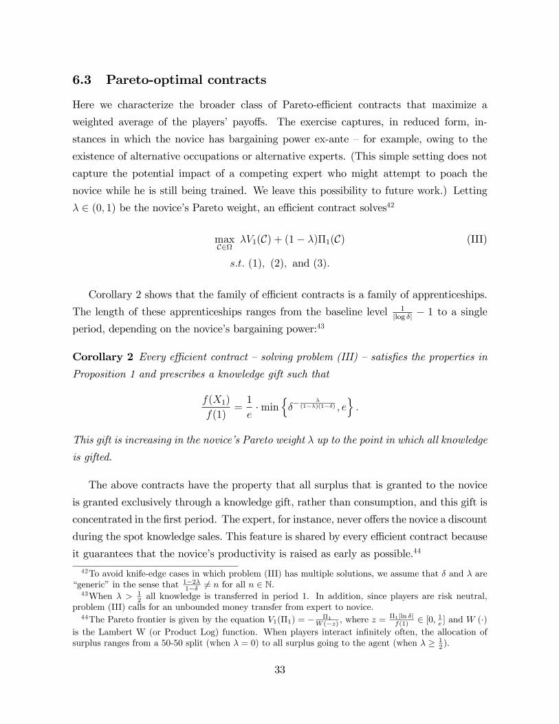
6.3 Pareto-optimal contracts

Here we characterize the broader class of Pareto-effi cient contracts that maximize a

weighted average of the players’ payoffs. The exercise captures, in reduced form, in-

stances in which the novice has bargaining power ex-ante — for example, owing to the

existence of alternative occupations or alternative experts. (This simple setting does not

capture the potential impact of a competing expert who might attempt to poach the

novice while he is still being trained. We leave this possibility to future work.) Letting

λ ∈ (0, 1) be the novice’s Pareto weight, an effi cient contract solves42

maxC∈Ω

λV1(C) + (1− λ)Π1(C) (III)

s.t. (1), (2), and (3).

Corollary 2 shows that the family of effi cient contracts is a family of apprenticeships.

The length of these apprenticeships ranges from the baseline level 1|log δ| − 1 to a single

period, depending on the novice’s bargaining power:43

Corollary 2 Every effi cient contract —solving problem (III) —satisfies the properties in

Proposition 1 and prescribes a knowledge gift such that

f(X1)

f(1)=

1

e·min

δ−

λ(1−λ)(1−δ) , e

.

This gift is increasing in the novice’s Pareto weight λ up to the point in which all knowledge

is gifted.

The above contracts have the property that all surplus that is granted to the novice

is granted exclusively through a knowledge gift, rather than consumption, and this gift is

concentrated in the first period. The expert, for instance, never offers the novice a discount

during the spot knowledge sales. This feature is shared by every effi cient contract because

it guarantees that the novice’s productivity is raised as early as possible.44

42To avoid knife-edge cases in which problem (III) has multiple solutions, we assume that δ and λ are“generic”in the sense that 1−2λ

1−δ 6= n for all n ∈ N.43When λ > 1

2 all knowledge is transferred in period 1. In addition, since players are risk neutral,problem (III) calls for an unbounded money transfer from expert to novice.44The Pareto frontier is given by the equation V1(Π1) = − Π1

W (−z) , where z = Π1|ln δ|f(1) ∈ [0, 1

e ] and W (·)is the Lambert W (or Product Log) function. When players interact infinitely often, the allocation ofsurplus ranges from a 50-50 split (when λ = 0) to all surplus going to the agent (when λ ≥ 1

2 ).

33

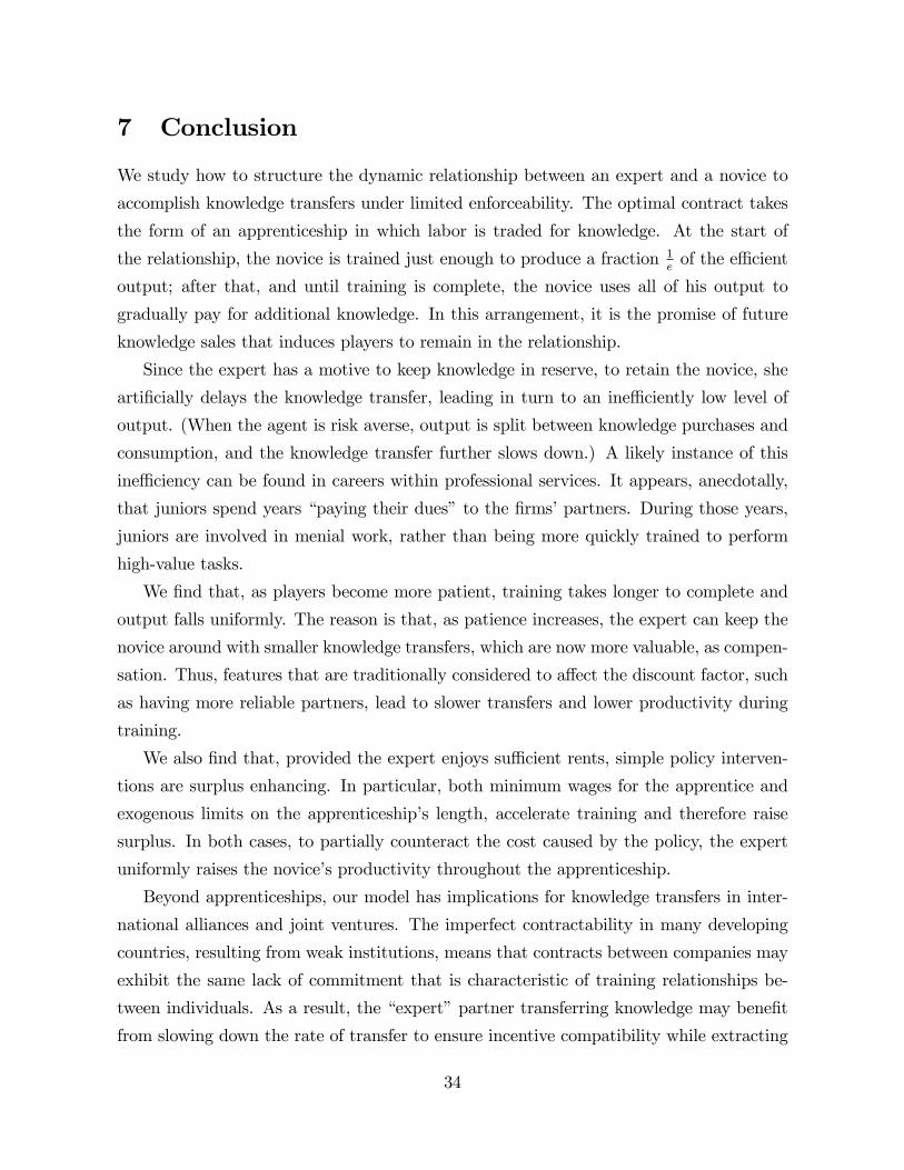
7 Conclusion

We study how to structure the dynamic relationship between an expert and a novice to

accomplish knowledge transfers under limited enforceability. The optimal contract takes

the form of an apprenticeship in which labor is traded for knowledge. At the start of

the relationship, the novice is trained just enough to produce a fraction 1eof the effi cient

output; after that, and until training is complete, the novice uses all of his output to

gradually pay for additional knowledge. In this arrangement, it is the promise of future

knowledge sales that induces players to remain in the relationship.

Since the expert has a motive to keep knowledge in reserve, to retain the novice, she

artificially delays the knowledge transfer, leading in turn to an ineffi ciently low level of

output. (When the agent is risk averse, output is split between knowledge purchases and

consumption, and the knowledge transfer further slows down.) A likely instance of this

ineffi ciency can be found in careers within professional services. It appears, anecdotally,

that juniors spend years “paying their dues”to the firms’partners. During those years,

juniors are involved in menial work, rather than being more quickly trained to perform

high-value tasks.

We find that, as players become more patient, training takes longer to complete and

output falls uniformly. The reason is that, as patience increases, the expert can keep the

novice around with smaller knowledge transfers, which are now more valuable, as compen-

sation. Thus, features that are traditionally considered to affect the discount factor, such

as having more reliable partners, lead to slower transfers and lower productivity during

training.

We also find that, provided the expert enjoys suffi cient rents, simple policy interven-

tions are surplus enhancing. In particular, both minimum wages for the apprentice and

exogenous limits on the apprenticeship’s length, accelerate training and therefore raise

surplus. In both cases, to partially counteract the cost caused by the policy, the expert

uniformly raises the novice’s productivity throughout the apprenticeship.

Beyond apprenticeships, our model has implications for knowledge transfers in inter-

national alliances and joint ventures. The imperfect contractability in many developing

countries, resulting from weak institutions, means that contracts between companies may

exhibit the same lack of commitment that is characteristic of training relationships be-

tween individuals. As a result, the “expert”partner transferring knowledge may benefit

from slowing down the rate of transfer to ensure incentive compatibility while extracting

34

maximum rents.

The model is highly tractable and can be used as a building block for other models in

which human capital acquisition is relevant. In future work, we expect to study training

hierarchies, where an expert can train a number of other agents who in turn can train

others. Also of interest would be to study, in the context of knowledge transfers between

firms, how other dimensions of the firms’interaction can be used to strengthen their rela-

tionship, and therefore accelerate training. An example is the use of cross-share holdings,

typical, for instance, of Japanese Keiretsus.

Finally, the empirical evidence we have mentioned is, by necessity, anecdotal. Future

empirical work is needed to study the extent to which training is ineffi ciently lengthy and

whether, as we suggest, patience slows down the rate at which knowledge is transferred.

35

Consu

mptio

n

Consu

mptio

n

Fig

ure 1

. Appren

ticeship

s with

concav

e utility

A. σ ∈

0.5

, 1, 1

.5; δ = 0

.9Lig

hter cu

rves co

rrespond to

hig

her σ

B. δ ∈

0.8

75, 0

.9, 0

.925; σ =

1Lig

hter cu

rves co

rrespond to

hig

her δ

C.

min /

(1) ∈

0.05, 0

.15, 0

.25; σ =

1; δ =

0.9

Lig

hter cu

rves co

rrespond to

low

er m

in

(δ is annual d

iscount fa

ctor; p

layers m

eet month

ly)

(years)

$ $

$

Outp

ut

Outp

ut

Consu

mptio

n

Outp

ut

ABC

11.6

13 14.2

(1)

(1)

(1)

0.3

(1)

0.2

6(1)

0.4

8(1)

0.2

5(1)

10.3

13

17.6

12.3

REFERENCES

1. Acemoglu, D. (1997). “Training and Innovation in an Imperfect Labour Market.”

Review of Economic Studies 64(3): 445-464.

2. Acemoglu, D., and J.-S. Pischke (1998). “Why Do Firms Train? Theory and Evi-

dence.”Quarterly Journal of Economics 113(1): 79-119.

3. Acemoglu, D., and J.-S. Pischke (1999a). “Beyond Becker: Training in Imperfect

Labour Markets.”Economic Journal 109(453): 112-142.

4. Acemoglu, D., and J.-S. Pischke (1999b). “The structure of wages and investment

in general training.”Journal of Political Economy 107(3): 539-572.

5. Albuquerque, R., and H. A. Hopenhayn (2004). “Optimal lending contracts and

firm dynamics.”Review of Economic Studies 71(2): 285-315.

6. Anton, J. J., and D. A. Yao (2002). “The sale of ideas: Strategic disclosure, property

rights, and contracting.”Review of Economic Studies 69(3): 513-531.

7. Baker, G., R. Gibbons, and K. Murphy (1994). “Subjective Performance Measures

in Optimal Incentive Contracts.”Quarterly Journal of Economics 109(4): 1125-

1156.

8. Bar-Isaac, H., and J.-J. Ganuza (2008). “Recruitment, training, and career con-

cerns.”Journal of Economics & Management Strategy 17(4): 839-864.

9. Barron, D., R. Gibbons, R. Gil, and K. J. Murphy (2015). “Reel Authority: Rela-

tional Adaptation in the Movie Industry.”Northwestern University, mimeo.

10. Becker, G. S. (1994[1964]). Human capital: A theoretical and empirical analysis

with special reference to education. University of Chicago Press.

11. Biais, B., T. Mariotti, G. Plantin, and J.-C. Rochet (2007). “Dynamic Security

Design: Convergence to Continuous Time and Asset Pricing Implications.”Review

of Economic Studies 74(2): 345-90.

12. Bruss, F. Thomas (1984). “A Unified Approach to a Class of Best Choice Problems

with an Unknown Number of Options.”Annals of Probability 12(3): 882-889.

37

13. Bull, C. (1987). “The Existence of Self-Enforcing Implicit Contracts.”Quarterly

Journal of Economics 102(1): 147-160.

14. Bulow, J., and K. Rogoff (1989). “Sovereign Debt: Is to Forgive to Forget?”Amer-

ican Economic Review 79(1): 43-50.

15. Burdett, K., and E. Smith (1996). “Education and Matching Externalities.” In

Acquiring Skills. Booth, A. L., and D. J. Snower, eds. Cambridge: Cambridge

University Press: 65-80.

16. Chang, C., and Y. Wang (1996). “Human Capital Investment under Asymmet-

ric Information: The Pigovian Conjecture Revisited.”Journal of Labor Economics

14(3): 505-519.

17. DeMarzo, P. M., and Y. Sannikov (2006). “Optimal Security Design and Dynamic

Capital Structure in a Continuous-Time Agency Model.”Journal of Finance 61(6):

2681-724.

18. DeMarzo, P. M., and M. J. Fishman (2007). “Optimal Long-Term Financial Con-

tracting.”Review of Financial Studies 20(6): 2079-2128.

19. Elbaum, Bernard (1989). “Why Apprenticeship Persisted in Britain But Not in the

United States.”Journal of Economic History 49(2): 337-349.

20. Garicano, L. (2000). “Hierarchies and the Organization of Knowledge in Produc-

tion.”Journal of Political Economy 108(5): 874-904.

21. Gergaud, O., V. Smeets, and F. Warzynski (2014). “Learning by Cooking and

Reputation Building: A French Recipe to Become a Top Chef.”KEDGE- Bordeaux

Business School, mimeo.

22. Goloboy, J. L. (2008). Industrial Revolution: People and Perspectives. ABC-CLIO.

23. Halac, M. (2012). “Relational contracts and the value of relationships.”American

Economic Review 102(2): 750-779.

24. Heckman, James (1971). “Three Essays on Household Labor Supply and the De-

mand For Market Goods.”Chapter 1, Ph.D. Dissertation. Princeton University.

38

25. Hörner, J., and A. Skrzypacz (2010). “Selling Information.” Cowles Foundation

Discussion Paper No. 1743.

26. Kahn, C., and G. Huberman (1988). “Two-Sided Uncertainty and “Up-or-Out”

Contracts.”Journal of Labor Economics 6(4): 423-444.

27. Katz, E., and A. Ziderman (1990). “Investment in General Training: The Role of

Information and Labour Mobility.”Economic Journal 100(403): 1147-1158.

28. Killingsworth, M. (1982) “Learning By Doing and Investment in Training: A Syn-

thesis of Two Rival Models of the Life Cycle.”Review of Economic Studies 49(2):

263-272.

29. Levin, J. (2003). “Relational Incentive Contracts.” American Economic Review

93(3): 835-857.

30. Levin, J., and S. Tadelis (2005). “Profit sharing and the role of professional part-

nerships.”Quarterly Journal of Economics 120(1): 131-171.

31. Li, J., and N. Matouschek (2013). “Managing conflicts in relational contracts.”

American Economic Review 103(6): 2328-2351.

32. Loewenstein, M. A., and J. R. Spletzer (1998). “Dividing the Costs and Returns to

General Training.”Journal of Labor Economics 16(1): 142-171.

33. MacLeod, W. B., and J. Malcomson (1989). “Implicit Contracts, Incentive Com-

patibility, and Involuntary Unemployment.”Econometrica 57(2): 447-480.

34. MacLeod, W. B., and J. Malcomson (1998). “Motivation and Markets.”American

Economic Review 88(3): 388-411.

35. Maister, D. H. (1993). Managing the Professional Service Firm. Free Press, New

York, NY.

36. Malcomson, J. M., J. W. Maw, B. McCormick (2003).“General training by firms,

apprentice contracts, and public policy.”European Economic Review 47(2): 197-

227.

37. McVeigh, S. (2006). Concert Life in London from Mozart to Haydn. Cambridge

University Press.

39

38. Prendergast, C. (1993), “The Role of Promotion in Inducing Specific Human Capital

Acquisition,”Quarterly Journal of Economics 108(2): 523-534.

39. Rayo, L. (2007). “Relational incentives and moral hazard in teams.” Review of

Economic Studies 74(3): 937-963.

40. Richter, A., M. Dickmann, and M. Graubner (2008). “Patterns of human resource

management in consulting firms.”Personnel Review 37(2): 184-202.

41. Rosen, S. (1972). “Learning and Experience in the Labor Market.” Journal of

Human Resources 7(3): 326-342.

42. Shaw, K. (1989). “Lifecycle Labor Supply with Human Capital Accumulation.”

International Economic Review 30(2): 431-456.

43. Smith, A. (1863). An Inquiry into the nature and causes of the Wealth of Nations.

J. R. M’Culloch., Ad. and Ch. Black.

44. Stevens, M. (1994). “Labour Contracts and Effi ciency in On-the-Job Training.”

Economic Journal 104(423): 408-419.

45. Thomas, J., and T. Worrall (1994). “Foreign direct investment and the risk of

expropriation.”Review of Economic Studies 61(1): 81-108.

46. Waldman, M. (1990). “Up-or-Out”Contracts: A Signaling Perspective.” Journal

of Labor Economics 8(2): 230-250.

47. Weiss, Y. (1972). “On the Optimal Lifetime Pattern of Labour Supply.”Economic

Journal 82(328): 1293-1315.

40

8 Appendix

Proof of Lemma 1. Let C ′ = 〈xt,m′t, d′t, w′t, ct〉∞t=1 be such that, for all t, d

′t = w′t = 0

and

m′t = mt + (1 + r) max dt−1f(Xt−1)− wt−1, 0+ min dtf(Xt)− wt, 0 ,

where d0 = w0 = X0 = 0.45 By construction, C ′ and C prescribe the same knowledgetransfers and overall payoffs Π1 and V1. Moreover, for all t,

Πt(C ′) = Πt(C) + (1 + r) max dt−1f(Xt−1)− wt−1, 0 ≥ Πt(C),

Vt(C ′) =

∞∑τ=t

δτ−tct = Vt(C), and Bt(C ′) = Bt(C) + max dtf(Xt)− wt, 0 .

We now show that C ′ satisfies the stage-1 constraints (1), (2), and (3). Constraint(1) is met because Πt(C ′) ≥ Πt(C) for all t. Constraint (3) is met because, for all t,mt ≤ (1 + r)Bt−1(C) implies

m′t ≤ (1 + r)Bt−1(C) + (1 + r) max dt−1f(Xt−1)− wt−1, 0+ min dtf(Xt)− wt, 0 ,

which in no greater than (1 + r)Bt−1(C ′). Constraint (2) is met because, for all t, eitherdt−1f(Xt−1)− wt−1 ≤ 0 and therefore the fact that C satisfies (2) in period t implies

Vt(C) ≥1

1− δf(Xt−1) +1

δBt−1(C) =

1

1− δ f(Xt−1) +1

δBt−1(C ′),

or dt−1f(Xt−1)−wt−1 > 0 and therefore the fact that C satisfies (5) in period t−1 implies

ct−1 + δVt(C)︸ ︷︷ ︸Vt−1(C)

≥ 1

1− δ f(Xt−1) + (1 + r)Bt−2(C)−mt−1

which is equivalent to Vt(C) ≥ 11−δf(Xt−1) + (1 + r)Bt−1(C ′).

Finally, we show that the stage-2 constraints (4), (5), and (6) are redundant. Con-

straint (4) is redundant because, given that d′t = w′t = 0 for all t, it is implied by constraint

45Namely, if in stage 2 the principal receives positive revenues (dtf(Xt)−wt > 0), add these revenues,with interest, to m′t+1; if in stage 2 the principal receives negative revenues (dtf(Xt)−wt < 0), subtractthese revenues from m′t. As a result, both contracts give the expert the same total revenues in presentdiscounted terms.

41

(1). Constraint (6) is redundant because, given that w′t = 0 for all t, it is implied by con-

straint (3). Constraint (5) is redundant because constraint (2) for period t+ 1 implies

δVt+1(C ′) = Vt(C ′)− ct ≥δ

1− δ f(Xt) +Bt(C ′),

which in turn implies Vt(C ′) ≥ 11−δf(Xt) + (1 + r)Bt−1(C ′)−mt, as desired.

Proof of Remark 1. That X1 > 0 and X2 − X1 > 0 follows from the fact that

both inequalities are necessary for the expert to make positive profits. We now show that

(1 + r)B1(C) = P (X2, X1). If (1 + r)B1(C) > P (X2, X1), the expert can relax (IC+L) by

reducingX1 by a small amount such that (1+r)B1(C) remains above P (X2, X1); if instead

(1 + r)B1(C) < P (X2, X1), the expert can relax (IC + L) by increasing X1 by a small

amount such that (1 + r)B1(C) remains below P (X2, X1). Finally, that X1 is transferred

for free follows noting that the only positive money transfer from expert to novice, m2, is

fully devoted to purchasing knowledge X2 −X1 rather than being used to pay for X1.

Proof of Lemma 2. Suppose toward a contradiction that contract C = 〈Xt,mt, ct〉∞t=1

solves problem (II) and yet has an infinite training phase —i.e. Xt < Xsup(C) for all t.The novice’s incentive constraints (2) require that, for all t,

1

1− δ f (Xt−1) + (1 + r)Bt−1(C) ≤ Vt(C) = (1 + r)Bt−1(C) +∞∑τ=t

δτ−t [f(Xτ )−mτ ]

and therefore∞∑τ=t

δτ−tmτ ≤∞∑τ=t

δτ−t [f(Xτ )− f (Xt−1)] . (12)

Now select a distant enough period k such that (1 + r)f (Xk−1) ≥ P (Xsup(C), Xk−1)

(which exists because Xk−1 must converge to Xsup(C) as k grows) and consider a newcontract C ′ = 〈X ′t,m′t, c′t〉

∞t=1 that is identical to C except for the following variables (in

words, C ′ asks the novice to save all period k−1 output and use these savings to purchase

at once, in period k, all knowledge Xsup(C)−Xk−1 that was eventually to be transferred):

1. X ′t = Xsup(C) for all t ≥ k.

2. c′k = 0 and c′t = f (Xsup(C)) + (1− δ) [(1 + r) f (Xk−1)−m′k] for all t > k (i.e. C ′

fully smooths consumption from period k onward).

3. m′k =∑∞

τ=k δτ−kmτ +

∑∞τ=k δ

τ−k [f (Xsup(C))− f(Xτ )] (i.e. in period k, the novice

42

is asked to pay a sum equal to all future discounted transfers in the original contract,

plus the present discounted value of the additional knowledge he receives in the new

contract) and m′t = 0 for all t > k.

We now show that C ′ meets all constraints. On the one hand, inequality (12) impliesthat

m′k ≤∞∑τ=k

δτ−k [f(Xτ )− f (Xt−1)] +∞∑τ=k

δτ−k [f (Xsup(C))− f(Xτ )] = P (Xsup(C), Xk−1) ,

which in turn implies that m′k ≤ (1+ r)f (Xk−1) and therefore all liquidity constraints (3)

are met.

On the other hand, from the definition ofm′k we obtain −m′k+∑∞

τ=k δτ−kf (Xsup(C)) =∑∞

τ=k δτ−k [−mτ + f(Xτ )], which implies that

Vk(C ′) = (1+r)[Bk−2(C) + f (Xk−1)]︸ ︷︷ ︸Bk−1(C′)

−m′k+∞∑τ=k

δτ−kf (Xsup(C)) = Vk(C)+(1+r)ck−1 ≥ Vk(C),

and that, for all t < k,

Vt(C ′) = (1+r)Bt−1(C)+k−1∑τ=t

δτ−t [f(Xτ )−mτ ]+δk−t

[ ∞∑τ=k

δτ−kf (Xsup(C))−m′k

]= Vt(C),

Consequently, the incentive constraints (2) are met for all t ≤ k. Moreover, since there

are no transactions after period k, all remaining incentive constraints are met as well.

Note, finally, that C ′ delivers a strictly higher payoffthan C (i.e. Π1(C ′) =∑k−1

τ=1 δτ−1mτ

+ m′k <∑k−1

τ=1 δτ−1mτ +

∑∞τ=t δ

τ−tmτ = Π1(C ′)), a contradiction.Proof of Remark 2. Let C = 〈Xt,mt, ct〉∞t=1 ∈ Ω be an arbitrary finite contract, with

final training period T, satisfying constraints (2) and (3). Select a bonus M , to be paid

in period T, such that

M =

T−1∑t=1

(1 + r)T−t [f(Xt)−mt]−∞∑t=T

δt−Tmt

(where the R.H.S. equals all output produced before period T net of all original money

transfers, expressed in period T dollars) and let contract C ′ = 〈Xt,m′t, c′t〉∞t=1 satisfy:

43

1. c′t = 0 for all t < T and c′t = f(XT ) + (1− δ)M for all t ≥ T (i.e. C ′ fully smoothsconsumption from period k onward).

2. m′t = (1 + r) f (Xt−1) for all t = 2, ..., T − 1, m′t = (1 + r) f (Xt−1) −M for t = T,

and m′t = 0 for all other t.

Notice that C ′ is a delayed-reward contract (and C ′ ∈ Ω). Moreover, from the defini-

tions of m′t and M ,

∞∑t=1

δt−1m′t =T−1∑t=1

δt−1f (Xt)− δT−1M =

∞∑t=1

δt−1mt,

and so both contracts prescribe the same total money transfers in present value.

That C and C ′ deliver the same payoffs Π1, V1 follows from the above observation

combined with the fact that both contracts prescribe the same output levels. That C ′

satisfies the liquidity constraints (3) follows directly from the definitions of c′t and m′t.

Finally, that C ′ satisfies the incentive constraints (2) follows from the fact that Vt(C ′) ≥Vt(C) for all t ≤ T (which in turn follows from the fact that c′t = 0 for all t < T ) and the

fact that all incentive constraints after period T are trivially met.

Proof of Lemma 3. Being a delayed-reward contract, C has the property that, for allt ≤ T,

Vt(C) = δT−tVT (C) = δT−t[

1

1− δf (XT ) +M

]. (13)

We now argue that, being a solution to (II), C has the property that in every periodt > 1 in which knowledge is transferred (Xt−1 < Xt), the novice’s incentive constraint

holds with equality:

1

1− δf (Xt−1) + (1 + r)f (Xt−1)︸ ︷︷ ︸Bt−1(C)

= δT−tVT (C). (14)

If instead the period-t constraint was met with strict inequality, the expert could raise

Xt−1 by a small amount while still satisfying the constraint (together with the requirement

that Xt−1 ≤ Xt), allowing the novice to produce additional output in period t− 1. Since

mt = (1 + r)f (Xt−1), this additional output would raise the expert’s revenue during t,

contradicting the optimality of C. (Notice that this change leaves all remaining incentiveconstraints unaffected because the novice’s continuation values Vt(C) depend only on XT

44

and M .)

We are now ready to show that, for any given t > 1, inequality (8) holds:

First, assume that Xt−1 = Xt. It follows that the R.H.S. of (8) is P (Xt, Xt−1) = 0 and

the L.H.S. is either mt + M · 1 t = T = (1 + r)f(Xt−1) ≥ 0 (if t ≤ T ) or mt = 0 (if

t > T ), as desired.

Second, assume that Xt−1 < Xt and further assume, toward a contradiction, that

inequality (8) fails. Suppose initially that t < T . Combining the incentive constraint for

period t with eq. (13) we obtain 11−δf (Xt) ≤ δT−tVT (C). In addition, since (8) fails we

must have (1 + r)f (Xt−1) < f (Xt) . From these two inequalities we obtain

1

δ(1− δ)f (Xt−1) <1

(1− δ)f (Xt) ≤ δT−tVT (C),

which contradicts eq. (14). Suppose finally that t = T. Since mT = (1 + r) f (XT−1)−M,

inequality mT +M < P (XT , XT−1) is equivalent to

1

δ(1− δ)f (XT−1) <1

1− δ f (XT ) ≤ VT (C),

which again contradicts eq. (14).

Proof of Proposition 1. Let D be the set of delayed-reward contracts. We proceedin two steps. First, we show that every optimal contract in D has the features in the

proposition. Second, we show that no contract outside D is optimal.Step 1. Consider an arbitrary contract C ∈ D (with bonusM and final period T ) that

solves the relaxed problem (II). From the proof of Lemma 3, eq. (14), in every period

t+ 1 such that Xt < Xt+1 we have

f (Xt) = (1− δ)δT−tVT (C). (15)

We now claim that

f(Xt) = min

(1− δ)δT−tVT (C), f(XT )for all t < T. (16)

We prove this claim by induction. That the claim is true for t = T − 1 follows from

noting that the novice’s incentive constraint for period T − 1 requires that f(XT−1) ≤(1 − δ)δVT (C), and whenever f(XT−1) < f(XT ) this constraint holds with equality (eq.

45

(15)). Now suppose the claim holds for t = T − n (n ∈ N). That the claim holds for

t = T − (n + 1) follows from noting that the novice’s incentive constraint for period

t requires that f(Xt) ≤ (1 − δ)δT−tVT (C), and whenever f(Xt) < f(XT ) we also have

f(Xt) < f(Xt+1) (since, by hypothesis, f(Xt+1) = min

(1− δ)δT−(t+1)VT (C), f(XT ))

and therefore the constraint must again hold with equality (eq. (15)).

From (16), and the fact that C ∈ D, we obtain

Π1(C) =

T−1∑t=1

δt−1 min

(1− δ)δT−tVT (C), f(XT )︸ ︷︷ ︸

δt−1f(Xt)

− δT−1M, (17)

where VT (C) = 11−δf (XT ) + M . The optimality of C requires that the above payoff is

maximized w.r.t. XT and M , subject to XT ≤ 1 and M ≥ 0. It follows that XT = 1.

We now observe that if M > (1 + r)f(1) there exists an alternative contract C ′ =

〈Xt,m′t, ct〉

∞t=1 in D that also solves problem (II) and that prescribes, in period T − 1, a

bonus M ′ = δ [M − (1 + r)f(1)] . Contract C ′ is identical to C except for the lower bonusand the fact that it ends one period sooner: m′T = 0 and m′T−1 = (1 + r)f(Xt−1) −M ′.

Notice also that δT−tVT (C) = δT−1−tVT−1(C ′) and thatM > (1+r)f(1) implies f(XT−1) =

f(1). Therefore, after manipulation of (17), we obtain:

Π1(C) =T−1∑t=1

δt−1 min

(1− δ)δT−tVT (C), f(1)− δT−1M

=T−2∑t=1

δt−1 min

(1− δ)δT−1−tVT−1, f(1)− δT−2M ′ = Π1(C ′).

In addition, we observe that M ≤ (1 + r)f(1) if and only if mT ≥ 0, which follows from

combining the definition of mT (namely, mT = (1 + r)f(XT−1) −M) with the fact thatf(XT−1) = min (1− δ)δVT (C), f(1).Consider now the expert’s original problem (I) in which the expert’s incentive con-

straints (1) are included. For contracts in D this constraint imposes the single additionalrestriction that mT ≥ 0 (otherwise the expert would walk away before paying −mT ),

which, as noted, is equivalentM ≤ (1 + r)f(1). It follows from the first observation in the

previous paragraph that problems (I) and (II) have the same value (asM can be repeatedly

reduced without lowering the expert’s payoff). In addition, from eq. (17), any contract

C ∈ D that solves problem (I) (for whichM ≤ (1+r)f(1) and so (1−δ)δT−tVT (C) ≤ f(1)

46

for all t < T ) delivers payoff

Π1(C) = (T − 1)δT−1 [f(1) + (1− δ)M ]− δT−1M.

Since this payoff is linear in M, and δ takes a generic value (namely, (1− δ)(T − 1) 6= 1),

it follows that M is either equal to zero (its lowest possible value) or equal to (1 + r)f(1)

(its highest possible one).

Finally, suppose contract C ∈ D solves problem (I). If M = 0, the prices stated in the

proposition are obtained by noting, from eq. (16), that f(Xt) = δf(Xt+1), and therefore

mt+1 = (1 + r)f(Xt) = P (Xt+1, Xt), for all t < T . If instead M = (1 + r)f(1), in the

last period of C no training takes place (as f(XT−1) = (1 − δ)δVT (C) = f(1)) and the

net money transfer is zero (as mT = (1 + r)f(1) −M = 0). As a result, this contract is

identical to a contract with M = 0, the same output and money transfers for t < T , and

that ends in period T − 1.

Step 2. Consider a contract C /∈ D and assume toward a contradiction that C solves theoriginal problem (I). From the proof of Remark 2, there is a contract C ′ ∈ D that solves therelaxed problem (II) (as problems (I) and (II) have the same value) and that prescribes the

same output levels as C. Given the output levels prescribed by these two contracts, duringthe training phase C ′ simultaneously maximizes each of the novice’s continuation payoffsVt (because consumption is delayed) and minimizes each of the novice’s cash balances

(1 + r)Bt−1 (because no savings beyond a single period are allowed). Moreover, since

C does not share this feature, it follows that under C ′ the novice’s incentive constraintis slack during at least one period t ≤ T . Consequently, C ′ fails to satisfy eq. (16), acontradiction.

Proof of Proposition 2. By substituting for the value of T (X1) in the objective of

problem (10), and multiplying this objective by the constant |log δ|f(1)

, problem (10) simplfies

to

maxX1≥0

log

[f (1)

f (X1)

]· f(X1)

f (1).

Since the average logarithm log(z)z

is uniquely maximized at z = e, the optimal gift X1

uniquely satisfies f(X1)f(1)

= 1e.

Proof of Corollary 1. Remark 2 and Lemma 3 remain valid under a minimum wage af-

ter two modifications.46 First, a delayed-reward contract C with length T is now defined as46It is also straightforward to verify that every optimal contract is finite.

47

one that, until graduation, grants the novice the smallest allowable consumption wmin each

period. As a result, the expert obtains gross revenues equal to (1 + r) [f(Xt−1)− wmin],

rather than (1 + r)f(Xt−1), during each period t = 2, ..., T. Second, in such a delayed-

reward contract, the novice’s incentive constraint for period t = 2, ..., T is 11−δf(Xt−1) +

(1 + r) [f(Xt−1)− wmin] ≤ Vt(C), where VT (C) = 11−δf(XT ) + M and Vt(C) is obtained

recursively from

Vt(C) = wmin + Vt+1(C) for t < T.

As a result, equation (14) in the proof of Lemma 3 is replaced by f(Xt) − wmin =

(1− δ)δT−tVT (C) − δT−twmin.

Other than these modifications, the proof of the present Corollary is identical to the

proof of Proposition 1, with equation (16) replaced by

f(Xt)− wmin = min

(1− δ)δT−tVT (C)− δT−twmin, f(XT )− wmin

for all t < T.

Proof of Proposition 3. After substituting for T (X1, wmin) and multiplying the

objective by ln(1+r)f(1)−wmin , problem (11) simplifies to

maxX1≥0

ln

[f (1)− wmin

f (X1)− wmin

]· f(X1)− wmin

f (1)− wmin

,

which is uniquely solved when f(X1)−wminf(1)−wmin = 1

e. Consequently, the length of the appren-

ticeship satisfies

T (X1, wmin)− 1 = ln

[f (1)− wmin

f (X1)− wmin

]· [ln (1 + r)]−1 =

1

|log δ| .

Finally, since net output f (Xt)− wmin grows at rate r during training, we obtain

f (Xt)− wmin

f (1)− wmin

=(1 + r)t−1

efor all t < T (X1, wmin),

which implies that f (Xt) is increasing in wmin for all t < T (X1, wmin).

Proof of Proposition 4. For a fixed contract duration T, the expert’s problem consists

in finding consumption and output paths (ct, yt)T−1t=1 (from period T onward the novice

48

produces and consumes f(1)). These paths solve:47

max(ct,yt)

T−1t=1

T−1∑t=1

δt−1 [yt − ct] +T−1∑t=1

λt

[Vt −

1

1− δu (yt)

],

where λt is the Lagrange multiplier for the period t incentive constraint, Vt =∑

τ≥t δτ−tu (cτ ),

and the output path is constrained to be nondecreasing and weakly below f(1).We begin

by ignoring these latter two constraints. In the resulting relaxed problem, all incentive

constraints bind (otherwise profits can be raised by raising yt) and the first-order order

conditions for ct and yt deliver, respectively:∑t

τ=1 λτδt−τu′ (ct) = δt−1 and λt = (1−δ)δt−1

u′(yt).48

After combining these two equalities, and rearranging terms, we obtain ct = (1 − δ) 1σYt.Moreover, since the Inada condition u′(0) = ∞ implies that yt > 0 for all t < T, the

resulting consumption path is increasing.

It remains to show that focusing on the above relaxed problem is appropriate. On

the one hand, that (yt)T−1t=1 is nondecreasing follows from the fact that

11−δu (yt) = Vt and,

since (ct)T−1t=1 is increasing, so is (Vt)

T−1t=1 . On the other hand, that (yt)

T−1t=1 is weakly below

f(1) follows from the fact that setting yt = f(1) for some t < T is equivalent to reducing

the contract’s duration T from the outset.

Proof of Corollary 2. Define a relaxed problem (IV) identical to (III) except that the

expert’s incentive constraints (1) are ignored. We begin by observing that the claims in

Lemmas 2, 3 and Proposition 1 remain valid for every effi cient contract (with problem (III)

replacing problem (I) and problem (IV) replacing problem (II)). To see why, notice that

the proof of each of these results is constructed by showing that any contract lacking the

desired properties is Pareto-dominated by a contract (delivering a strictly higher payoff

for the expert and a weakly higher payoff for the novice) that does satisfy them.

Once we restrict to contracts satisfying Proposition 1, the objective in (III), as a

function of X1, becomes

λP (X1, 0)︸ ︷︷ ︸V1

+ (1− λ)[T (X1)− 1] f(X1)︸ ︷︷ ︸,Π1

where T (X1)−1 satisfies eq. (9). Ignoring the integer constraint for T (X1), this objective

47We have assumed that the expert does not use a bonus (M = 0). The proof that doing so is optimalis omitted for brevity and is available upon request.48It also follows from the strict concavity of u that the first-order conditions are suffi cient for optimality

of the two paths.

49

is uniquely maximized when f(X1)f(1)

= 1e·min

δ−

λ(1−λ)(1−δ) , e

.

50

CENTRE FOR ECONOMIC PERFORMANCE Recent Discussion Papers

1411 João Paulo Pessoa International Competition and Labor Market Adjustment

1410 Claudia Olivetti Barbara Petrongolo

The Evolution of Gender Gaps in Industrialized Countries

1409 Quoc-Anh Do Kieu-Trang Nguyen Anh N. Tran

One Mandarin Benefits the Whole Clan: Hometown Favoritism in an Authoritarian Regime

1408 Caroline J. Charpentier Jan-Emmanuel De Neve Jonathan P. Roiser Tali Sharot

Models of Affective Decision-making: How do Feelings Predict Choice?

1407 Johannes Boehm Swati Dhingra John Morrow

Swimming Upstream: Input-output Linkages and the Direction of Product Adoption

1406 Felix Koenig Alan Manning Barbara Petrongolo

Reservation Wages and the Wage Flexibility Puzzle

1405 Gianluca Benigno Luca Fornaro

Stagnation Traps

1404 Brian Bell Stephen Machin

Minimum Wages and Firm Value

1403 Gene M. Grossman Elhanan Helpman Ezra Oberfield Thomas Sampson

Balanced Growth Despite Uzawa

1402 Emanuele Forlani Ralf Martin Giordano Mion Mirabelle Muûls

Unraveling Firms: Demand, Productivity and Markups Heterogeneity

1401 Holger Breinlich The Effect of Trade Liberalization on Firm-Level Profits: An Event-Study Approach

1400 Richard V. Burkhauser Jan-Emmanuel De Neve Nattavudh Powdthavee

Top Incomes and Human Well-Being Around the World

1399 Rabah Arezki Thiemo Fetzer

On the Comparative Advantage of U.S. Manufacturing: Evidence from the Shale Gas Revolution

1398 Adriana Kocornik-Mina Thomas K.J. McDermott Guy Michaels Ferdinand Rauch

Flooded Cities

1397 Lorenzo Caliendo Giordano Mion Luca David Opromolla Esteban Rossi-Hansberg

Productivity and Organization in Portuguese Firms

1396 Richard Murphy Gill Wyness

Testing Means-Tested Aid

1395 Zack Cooper Stuart Craig Martin Gaynor John Van Reenen

The Price Ain’t Right? Hospital Prices and Health Spending on the Privately Insured

1394 Hannes Schwandt Amelie Wuppermann

The Youngest Get the Pill: Misdiagnosis and the Production of Education in Germany

1393 Yatang Lin Yu Qin Zhuan Xie

International Technology Transfer and Domestic Innovation: Evidence from the High-Speed Rail Sector in China

1392 Robin Naylor Jeremy Smith Shqiponja Telhaj

Graduate Returns, Degree Class Premia and Higher Education Expansion in the UK

1391 Marc Fleurbaey Hannes Schwandt

Do People Seek To Maximize Their Subjective Well-Being?

The Centre for Economic Performance Publications Unit Tel 020 7955 7673 Fax 020 7404 0612

Email info@cep.lse.ac.uk Web site http://cep.lse.ac.uk