ISSN 2042-2695

CEP Discussion Paper No 1692

May 2020

All These Worlds are Yours, Except India:

The Effectiveness of Cash Subsidies to Export in Nepal

Fabrice Defever

José-Daniel Reyes

Alejandro Riaño

Gonzalo Varela

Abstract This paper studies the impact of a `textbook' ad-valorem export subsidy on firm-level export performance.

The Cash Incentive Scheme for Exports (CISE) program offered by the government of Nepal offers a cash

subsidy to firms exporting a select group of products to countries other than India. Using customs

transactions data combined with subsidy disbursements at the firm level from 2011 to 2014, we estimate

the impact of the subsidy on exports of targeted and non-target product-destination combinations and their

extensive and intensive margins. We employ a range of doubly-robust matching estimators to control for

the non-random selection of exporters into the scheme. We find that subsidized firms increased their

exports of targeted product-destinations relative to firms in the control group and that this rise is fully

accounted for by the extensive margin: a higher number of targeted products exported and foreign markets

served. We do not find any significant changes along the intensive margin nor among non-targeted

product-destination combinations. While our results show that the CISE scheme fomented export

diversification, its limited impact on total exports and high fiscal cost call into question its effectiveness.

Key words: export subsidies, export diversification, export margins, least developed countries, special and

differential treatment for developing countries, Nepal

JEL Codes: F13; F14; F61; O24

This paper was produced as part of the Centre’s Trade Programme. The Centre for Economic Performance

is financed by the Economic and Social Research Council.

This paper is a product of our discussion with Swarnim Wagle (Member of the National Planning

Commission of Nepal), whose guidance and support is gratefully acknowledged. We would also like to

thank Purushottam Ojha and Chandan Sapkota for clarifying our understanding about specific details of

the CISE export subsidy scheme. All remaining errors are ours. Aldo Pazzini provided excellent research

assistance. We would like to thank Isabelle Mejean (the Editor) an anonymous Associate Editor and one

referee for their valuable comments. We would also like to thank Emek Basker, Ana Fernandes, Sourafel

Girma, Caio Piza, Irani Arraiz, Camilo Umana-Dajud and participants at the 6th InsTED workshop and the

Ljubljana Empirical Trade Conference for their comments and suggestions, which have greatly improved

the paper. The findings, interpretations, and conclusions expressed in this paper are entirely those of the

authors. They do not represent the view of the World Bank, its Executive Directors, or the countries they

represent.

Fabrice Defever, City, University of London, CESifo and Centre for Economic Performance,

London School of Economics. José-Daniel Reyes, The World Bank. Alejandro Riaño, City, University of

London, GEP, CFCM and CESifo. Gonzalo Varela, The World Bank.

Published by

Centre for Economic Performance

London School of Economics and Political Science

Houghton Street

London WC2A 2AE

All rights reserved. No part of this publication may be reproduced, stored in a retrieval system or

transmitted in any form or by any means without the prior permission in writing of the publisher nor be

issued to the public or circulated in any form other than that in which it is published.

Requests for permission to reproduce any article or part of the Working Paper should be sent to the editor

at the above address.

F. Defever, J-D. Reyes, A. Riaño and G. Varela, submitted 2020.

1 Introduction

While export subsidies are ubiquitous across the world, according to the World Trade Organization,

there are fewer empirical studies investigating them than almost any other instrument of commercial

policy (WTO, 2006). As a case in point, the chapter by Bown and Crowley (2016) in the Handbook

of Commercial Policy edited by Bagwell and Staiger entitled “The Empirical Landscape of Trade

Policy” does not consider export subsidies at all (see footnote e, page 7) and the chapter on

“Subsidies and Countervailing Duties” by Lee (2016) in the same handbook only reviews theoretical

research on this topic.

We contribute to bridge this gap in the literature by evaluating how a ‘textbook’ ad-valorem

export subsidy affects firm-level export performance. To the best of our knowledge, we are the

first to ever do so.1 We take advantage of the Cash Incentive Scheme for Exports (CISE)—a

program introduced by the government of Nepal in 2012 to increase exports and foster export

diversification—to achieve our goal. CISE offers firms ad-valorem cash payments on the basis of

their sales of a select group of products exported to countries other than India.

There are two main reasons behind the dearth of empirical work on export subsidies that we

overcome effectively in this paper. First, export subsidies take a wide variety of forms, such as con-

cessions and exemptions on a variety of tax levies; access to public utilities at below-market prices

and soft loans granted to firms in special economic zones; export credit guarantees; co-financing

grants for training, investment in physical capital, R&D, and business development conditioned

on export performance, among others.2 This remarkable degree of heterogeneity combined with

the imposition of different eligibility requirements often makes it difficult to systematically identify

which firms are subsidized and to what extent.

In contrast, the CISE scheme is a simple, well defined, ad-valorem cash subsidy granted on

the basis of exports of a list of products sold anywhere but India. Our data provides information

on which firms are subsidized, how much cash they receive and which products they export and

1Earlier work on export subsidies relied on country- or industry-level data; see e.g. Balassa (1978) and the papersreviewed in Rodrik (1995). The fact that there are large difference across firms—even within narrowly-definedindustries—is well established. As we discuss in more detail below, the variation afforded by the firm-level dataallows us to identify the impact of export subsidies in a way that would not be feasible with more aggregate data atthe sector or product levels.

2Farole and Akinci (2011), Wang (2013), Defever and Riano (2017), and Defever et al. (2019) study a broad rangeof incentives—primarily tax exemptions—offered in special economic zones; Felbermayr and Yalcin (2013) investigateexport credit guarantees; Gorg et al. (2008) and Cadot et al. (2015) study co-financing grants provided to exporters.

1

where. This is a crucial advantage relative to existing papers in the literature. Defever and Riano

(2017) and Defever et al. (2019) identify firms that are eligible to receive a broad range of subsidies

conditioned on their export intensity being above a given threshold or their location in special

economic zones, but do not observe which firms enjoy the different incentives available. Kalouptsidi

(2018) does not observe which firms are subsidized either, and therefore infers the presence and

magnitude of subsidies received by shipbuilders in China by means of a structural model. Some

manufacturing surveys provide information on subsidies received by individual firms, but bundle

together disbursements from several programs with different objectives and eligibility requirements

(Girma et al., 2009; Helmers and Trofimenko, 2013).

The second reason for the paucity of data and empirical work on export subsidies is that they

are prohibited by the WTO Agreement on Subsidies and Countervailing Measures (ASCM). This

gives governments the incentive to not report export subsidies in order to avoid being challenged

by other WTO members and potentially face countervailing duties; see e.g. WTO (2006) and

Haley and Haley (2013). Since Nepal is a WTO member and one of 47 countries classified by the

United Nations (UN) as a Least Developed Country (LDC), it is not subject to the disciplines

of the ASCM due to the principle of Special and Differential Treatment for Developing Countries

(SDT).3 This exemption allows it to offer an export subsidy like the CISE scheme without risking

retaliation. There is very limited research on the SDT principle, and most of the empirical work in

this area focuses on the role of non-reciprocal preferences granted by developed countries (Ornelas,

2016); instead we examine whether the use of otherwise prohibited export subsidies can help poorer

countries to export more. Similarly, we see our paper as complementary to the theoretical work

investigating the normative properties of the WTO’s subsidy rules (Bagwell and Staiger, 2006; Lee,

2016).

In addition to being the first paper to evaluate the impact of an ad-valorem export subsidy

on firm-level export performance, our paper makes two important contributions to the flourishing

literature that evaluates the effect of export promotion policies on export outcomes (Alvarez and

3See Article 27.2.(a) of the ASCM. The SDT principle also allows LDCs to, among other things, offer subsidiesto agricultural products, investment and to encourage diversification away from illegal crops which are exemptfrom domestic support reduction commitments; have a higher de minimis percentage of Aggregate Measurement ofSupport (AMS); use restrictive import measures for balance-of-payment purposes and have longer transition periodsto implement WTO commitments. Additional examples can be found here: https://www.wto.org/english/tratop_e/devel_e/teccop_e/s_and_d_eg_e.htm.

2

Crespi, 2000; Bernard and Jensen, 2004; Volpe Martincus and Carballo, 2008; Gorg et al., 2008;

Volpe Martincus and Carballo, 2010a; Cadot et al., 2015; Van Biesebroeck et al., 2015, 2016; Munch

and Schaur, 2018). While the existing literature studying the work of export promotion agencies

(EPA) has focused exclusively on middle-income and developed countries (see Table 1 of Van

Biesebroeck et al., 2016), we conduct the first impact evaluation of export promotion policies in a

least developed country. This is an important contribution because due to the limited integration

of LDCs in global trade, one of the UN’s Sustainable Development Goals is to double LDCs’ share

of global trade by 2020.

The second contribution pertains to the specific policy instrument we evaluate. The objective

of EPAs is to lessen informational frictions that affect international transactions more severely than

domestic ones by offering a wide range of services to exporters such as logistic help to meet foreign

buyers; provision of market research; information on customs clearance, shipping and insurance; co-

financing of export business plans, and many more. These interventions could affect the fixed and

variable costs of trade faced by exporters in different ways. The CISE subsidy, on the other hand,

simply increases the marginal revenue of firms exporting a well defined set product-destination

pairs. This allows us to establish theoretical predictions that we then corroborate in our empirical

work.

Nepal has a GDP per capita close to the median among LDCs and shares two key traits

that characterize export performance among these countries—a large trade deficit and a highly

concentrated export basket (Nicita and Seiermann, 2016; Papageorgiou and Spatafora, 2012). The

trade policy instrument we investigate—cash subsidies granted to exports of specific products sold in

certain destinations—is also commonly used by developing countries, particularly Nepal’s neighbors.

Bangladesh, for instance, offers these subsidies (with ad-valorem rates as high as 30%) to a wide

range of products such as frozen shrimp, jute and straw products, leather goods and garments

among others. India also provides cash incentives ranging from 2 to 5% of exports to more than

100 products under its Merchandise Exports Incentive Scheme with subsidy rates varying according

to the country to which the goods are sold to.4 Both of these features lend credibility to the external

validity of our results.

4See http://www.bangladeshcustoms.gov.bd/trade_info/export_incentives and http://dgft.gov.in/

sites/default/files/pn0617.pdf.

3

In order to guide our empirical analysis, we make use of the model of multi-product, multi-

destination exporters of Bernard et al. (2011). We derive predictions about how an ad-valorem

subsidy granted to firms exporting a subset of products to countries other than India (which we

refer to as ‘the rest of the world’ hereafter) affects firms’ exports and their extensive (number of

product-destinations exported) and intensive (average exports per product-destination) margins.

We add a fixed administrative cost that firms incur in order to receive the subsidy to the model in

order to accommodate the low participation of eligible firms in the scheme that we observe in the

data.

Our theoretical framework delivers the following predictions. Since the marginal cost of pro-

duction and market access are independent across all product-destination pairs exported by any

given firm, it follows that the subsidy only affects exports of eligible products sold in the rest of the

world. The existence of an administrative cost, in turn, implies that only firms for which sales of

targeted product-destinations are sufficiently important find it profitable to apply to the scheme.

Conditional on participating in the program, the model predicts that subsidized firms increase their

exports of targeted products sold in the rest of the world because the marginal revenue firms from

selling these varieties increases.

Turning to the effect of the subsidy on export margins, the assumption that both productivity

and product attributes are drawn from Pareto distributions means that the expansion of exports

is fully accounted for by the extensive margin—i.e. by an increase in the number of targeted

product-destination pairs that firms export. Firms’ average exports per product-destination are

unaffected by the subsidy because the higher sales of existing varieties are exactly balanced by the

lower sales of less profitable ones that firms only begin to export after they receive the incentive.

Since cost linkages across products within the same firm feature prominently in the theoretical

literature on multi-product exporters (Eckel and Neary, 2010; Mayer et al., 2014; Nocke and Yeaple,

2014; Arkolakis et al., 2016), we also investigate empirically whether the CISE subsidy affects

subsidized firms’ exports of non-targeted product-destinations: i.e. sales of any product to India

and of products not included in CISE to the rest of the world.

To carry out our empirical analysis we combine customs transaction data for the period 2011-

2014 with information on subsidy payments to individual firms. There are 24 industrial and 7

agricultural products included in the CISE scheme which are of crucial importance for Nepal’s

4

exports. In 2011, the year before the subsidy was introduced, the products included in the scheme

accounted for 41% of aggregate exports, two-thirds of which was sold outside India; in the same

year, 70% of all Nepalese exporters carried out at least one export transaction eligible to receive

the subsidy.

The main obstacle we face to estimate the causal impact of the CISE subsidy on export perfor-

mance is the non-random selection of firms into the treatment. We tackle this problem by combining

the doubly-robust matching estimator proposed by Wooldridge (2007) with a linear panel model

with firm and year fixed effects. The identification assumption underlying our matching estima-

tors is that observable pre-treatment characteristics control for firms’ decision to participate in the

subsidy program while firm and year fixed effects control for time-invariant factors and aggregate

shocks affecting export performance respectively. Evidence from field interviews with exporters

conducted by Pazzini et al. (2016) reveal that the low participation of eligible firms in the scheme

is mainly due to lack of awareness about the program among exporters, red tape and coordination

problems among the different government bodies involved in the administration of the program.

Our theoretical framework, in turn, predicts that exporters who stand to gain the most to over-

come the administrative barriers—i.e. larger firms for which sales of targeted product-destinations

account for a higher share of their sales—are more likely to receive the subsidy. This is exactly

what we find when we estimate the propensity score. Crucially, the high uncertainty involved in the

allocation of the subsidy ensures that even after controlling for the observable characteristics driv-

ing firms’ participation, there are still several eligible exporters that did not receive the subsidy but

which are otherwise very similar to treated firms in terms of their pre-treatment characteristics—to

proxy for the latter’s counterfactual outcomes.

Our results lend support to the predictions derived from our theoretical framework and show

that the CISE scheme has been most effective in encouraging firms’ export diversification—particularly

along the geographic dimension. More specifically, we find that, relative to the control group, firms

that received the subsidy increase the number of destinations (other than India) they sell to by

10-12%, and the number of products included in the CISE scheme they export by 6-7%. The impact

on the extensive margin of exports we estimate is very similar to what the literature evaluating

the effect of support services provided by export promotion agencies finds in developing countries

(Alvarez and Crespi, 2000; Volpe Martincus and Carballo, 2008, 2010a; Cadot et al., 2015). Consis-

5

tent with our theory, we do not find any significant impact of the subsidy on the intensive margin

of exports—i.e. on average exports per product, destination and product-destination. Furthermore,

and consistent with the assumption that the cost of production and market access are independent

across the product-destination pairs exported by a given firm, we do not find any evidence of the

subsidy affecting firms’ exports to India (regardless of whether the products are included in the

CISE scheme or not) nor on sales of non-eligible products sold in the rest of the world.

We find a positive, yet not precisely estimated, impact of the subsidy on total export sales

of treated firms. Digging deeper into this reveals two key features that have weaken the impact

of the scheme: firms’ low participation rates and its broad scope in terms of the products being

incentivized. While the CISE scheme could potentially be available to three out of four Nepalese

exporters, only few of them obtained it and even fewer receive it more than once. Our results show,

however, that the subsidy only produces significantly positive effects on export sales when firms

receive the incentive repeatedly. The second problem is that the broad product coverage of the

scheme tends to attenuate its impact. For instance, we find that the positive results we estimate

are mainly driven by the exporters of textiles and clothing, while among we do not find significant

results for firms exporting other products included in the scheme.

While the scheme has succeeded in redirecting Nepalese exports towards the rest of the world,

the lack of a significant effect on firms’ total exports suggests the CISE scheme has not been

effective in achieving its objectives. This is all the more salient when we consider that the annual

expenditure on the scheme exceeds the entire budget of EPA in countries that are substantially

richer than Nepal (see Section 5 for more detail) and the tight constraints that Nepal faces on its

public finances after the disastrous earthquake that hit it in 2015, generating economic losses in

the order of 10 billion US dollars.5

The rest of the paper is organized as follows: Section 2 describes the CISE export subsidy, its

eligibility requirements and institutional characteristics. Section 3 introduces our data and provides

summary statistics on export patterns in Nepal and the usage of the CISE export subsidy. Section

4 establishes a set of predictions about the effects of the CISE subsidy on firms’ exports and their

extensive and intensive margins grounded on a workhorse model of trade with multi-product and

multi-destination exporters; Section 4 also lays out our empirical strategy to estimate the causal

5This is also the reason why we only have data until 2014 to conduct our empirical analysis.

6

effect of the CISE subsidy on firm-level export performance. Section 5 presents our results and

Section 6 concludes.

2 The Cash Incentive Scheme for Exports

The Cash Incentive Scheme for Exports (CISE) is an ad-valorem cash subsidy offered to firms by the

government of Nepal with the objective of increasing exports and fostering export diversification.

It is hard to find a country for which both of these goals are more pressing than Nepal (WTO,

2012). Fuelled by large inflows of remittances from abroad, Nepal’s chronically high trade deficit

has continued to worsen since 2000, reaching 24% of GDP in 2011.6 In the same year, only 5

HS 6-digit products accounted for one-third of its exports and 85% of its exports were sold to 5

countries, 80% of which were destined to India alone.

The subsidy is provided to firms on the basis of their exports of 24 industrial and 7 agricultural

products sold in countries other than India.7 Subsidy payments are disbursed by the Nepalese

Central Bank (Nepal Rastra Bank) on a ‘first come, first served’ basis upon receiving evidence that

payment for an export transaction in foreign exchange has been deposited in a Nepalese bank. The

initial budget allotted to the scheme in 2012 was 240 million Nepalese rupees (approximately 3.2

million US dollars), and was further increased to 300 million rupees in 2013. Across the three

years for which we have data (2012-2014), yearly disbursements have always been lower than the

scheme’s annual budget. This suggests that the low participation rate of firms in the scheme, which

we document in more detail in the next section, is not due to larger exporters claiming the subsidy

earlier in the year and crowding out smaller exporters once the scheme’s funding has ran out.8 The

subsidy is available both to direct exporters and “Export Trading Houses” (i.e. wholesalers), which

are required to transfer 50% of the cash payment to the producer of the good in question.9

The list of products included in CISE and their respective subsidy rates is presented in Table

1. The products included in the scheme were selected on the basis of the recommendations made

6This is a very high trade deficit, even among least developed countries. In 2011, only 9 out of 48 LDCs had atrade deficit higher than Nepal.

7What the Nepalese Customs Act Rules and Regulations refers to as “third countries”.8We do not find systematic differences in the seasonal export patterns of the products included in the CISE

scheme that would suggest that, everything else equal, exporters of certain products would be more likely to receivethe subsidy because they are more likely to apply for it earlier in the year before funding runs out.

9Our data, however, does not allow to distinguish direct exporters and wholesalers.

7

in the 2010 Nepal Trade Integration Strategy. The report, produced by the Ministry of Commerce

and Supply in consultation with Nepalese business leaders, used three key criteria to identify

products for which the government should prioritize export support: (i) current and potential

export performance; (ii) high domestic value added and (iii) socioeconomic impact.10

Table 1: Products Included in the Cash Incentive Scheme of Exports and Subsidy Rates

Industrial Products Agricultural Products2% subsidy rate 1% subsidy rate 1% subsidy rate

Processed coffee Ready-to-eat chow chow SeedsSemi-processed hides & skins Bran Cut flowersHandicraft & wooden craft Wheat flour FruitsCrust skin Polyester or viscous yarn VegetablesHandmade paper & rel. products Ready-made garments GingerProcessed honey Polyester textile yarn CardamomTea Vegetable fat/oil HerbsCarpet & woolen products TransferPashmina & silk products Ball pensProcessed herbs & essential oils Lentils

Precious & semi-precious jewelryGold & silver ornamentsTurmericDried ginger

Source: CISE 2070, Government of Nepal Ministry of Commerce and Ojha (2015).

There are two reasons that justify the exclusion of exports to India from the CISE scheme.

The first is that one of program’s goals is to promote the diversification of Nepalese exports—

particularly away from India. The second is the free movement of people and goods between India

and Nepal, which has been in place since 1950 following the signature of the India-Nepal Treaty of

Peace and Friendship (Sharma, 2015). The Ministry of Finance’s concern was that extending the

subsidy to exports to India would encourage firms to ship their products there, claim the subsidy

and then bring the goods back to be sold in Nepal—thereby subsidizing domestic sales instead of

actual exports.11

10The first criteria was assessed by means of products’ export values and growth rates in 2008, the size of importmarkets and import tariffs faced by Nepalese exporters. The third considers a sector’s total employment, femaleparticipation and overall importance in poorer regions.

11To further ensure that no subsidies are granted to exports to India, the CISE regulations stipulate that exporttransactions have to be denominated in convertible currencies. Doing so effectively excludes sales invoiced in Indian

8

The CISE subsidy was first introduced by the Ministry of Finance in the Public Statement

on Income and Expenditure for the 2010-11 fiscal year in November 2010, but the scheme only

began to operate in 2012 due to delays in the preparation of guidelines and regulations (Sapkota,

2011). In its inception, the CISE scheme required export shipments to incorporate at least 30%

of domestic value-added and subsidy rates were increasing in the share of local content. This

aspect of the program was quickly reformed in 2013 following complaints from exporters about

the administrative burden involved in the calculation of domestic value-added.12 Exporters, for

instance, were required to fill new value-added assessments for every export transaction for which

they claimed the subsidy. This procedure was made even more cumbersome due to the fact that

different government agencies involved in the administration of the scheme, such as the Department

of Customs and the Ministry of Industry, use different methodologies to calculate domestic value

added (Sapkota, 2011).

Field interviews with Nepalese exporters conducted by Pazzini et al. (2016) reveal that the

main barriers that exporters face to take advantage of the incentive are a widespread lack of

awareness about the scheme as well as lengthy and complex administrative procedures involved in

claiming the subsidy. One of the interviewees vividly likened the process involved in obtaining the

subsidy to “being invited for dinner and then asked to climb through the roof after knocking on

the door.” Interviewees, however, do not mention political connections nor the need to pay bribes

to government officials as being significant factors precluding their participation in the scheme. It

follows that only eligible exporters for which subsidy payments are sufficiently large would find it

profitable to face the red-tape associated with receiving the incentive. Even then, many eligible firms

did not received subsidies either because they did not apply for them or because their application

was not approved by the government authorities in charge of the scheme.

rupees, which are deemed to be non-convertible by the Nepalese Central Bank.12It is important to note that the products selected for the scheme in 2013 are characterized by a high share of

domestic value added. All beneficiaries of the subsidy in 2012 exported products included in the list in Table 1. Whilethe Ministry of Industry reviews the list of products to be included in the scheme and their subsidy rates every year,no changes have been made to the program since 2013.

9

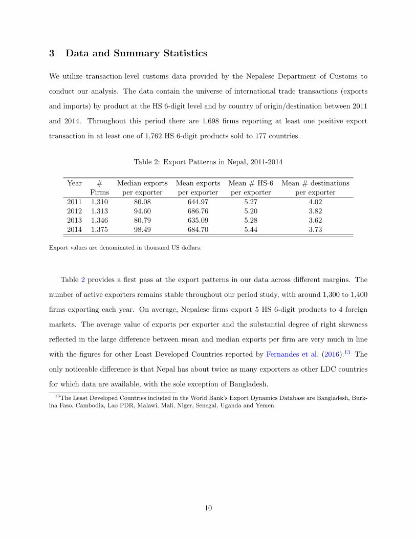
3 Data and Summary Statistics

We utilize transaction-level customs data provided by the Nepalese Department of Customs to

conduct our analysis. The data contain the universe of international trade transactions (exports

and imports) by product at the HS 6-digit level and by country of origin/destination between 2011

and 2014. Throughout this period there are 1,698 firms reporting at least one positive export

transaction in at least one of 1,762 HS 6-digit products sold to 177 countries.

Table 2: Export Patterns in Nepal, 2011-2014

Year # Median exports Mean exports Mean # HS-6 Mean # destinationsFirms per exporter per exporter per exporter per exporter

2011 1,310 80.08 644.97 5.27 4.022012 1,313 94.60 686.76 5.20 3.822013 1,346 80.79 635.09 5.28 3.622014 1,375 98.49 684.70 5.44 3.73

Export values are denominated in thousand US dollars.

Table 2 provides a first pass at the export patterns in our data across different margins. The

number of active exporters remains stable throughout our period study, with around 1,300 to 1,400

firms exporting each year. On average, Nepalese firms export 5 HS 6-digit products to 4 foreign

markets. The average value of exports per exporter and the substantial degree of right skewness

reflected in the large difference between mean and median exports per firm are very much in line

with the figures for other Least Developed Countries reported by Fernandes et al. (2016).13 The

only noticeable difference is that Nepal has about twice as many exporters as other LDC countries

for which data are available, with the sole exception of Bangladesh.

13The Least Developed Countries included in the World Bank’s Export Dynamics Database are Bangladesh, Burk-ina Faso, Cambodia, Lao PDR, Malawi, Mali, Niger, Senegal, Uganda and Yemen.

10

Table 3: Composition of Export Value by Product Type and Destination in 2011 (%)

Destination { Product Included Not included Totalin CISE in CISE

India 15.4 51.3 66.7Rest of the World 25.6 7.7 33.3

Total 41.0 59.0 100

Table 3 decomposes Nepal’s exports in 2011—the year before the CISE export subsidy started

to operate—according to the scheme’s product and destination eligibility requirements. Two key

insights emerge from Table 3. As we have noted before, India accounts for two-thirds of aggregate

exports, and most of these are of products that are not included in the CISE scheme. Products

listed in CISE are very important in Nepal’s export basket and are sold primarily outside India.

Thus, there is substantial overlap between the product and destination eligibility criteria of the

CISE scheme.

Table 4: Eligibility, Usage, and CISE Subsidy Disbursements

Year # # Eligible # Exporters # First time Total subsidyExporters exporters receiving subsidy disbursements

subsidy recipient (mill. US dollars)

2011 1,310 917 - - -2012 1,313 878 28 28 1.5702013 1,346 912 57 42 1.8052014 1,375 921 151 103 3.813

Eligible exporters are those that have conducted at least one export transaction of a product listed in CISE to acountry other than India in a given year. The CISE subsidy is not in place in 2011.

We next examine the amount of subsidies disbursed throughout our period of analysis using

data provided by the Central Bank of Nepal, the entity in charge of paying out the subsidies to

firms. These data inform us of the total amount of cash that exporters receive in a given fiscal

year, and therefore, do not allow us to identify the individual export transactions for which a firm

receives the subsidy. Table 4 shows that approximately two-thirds of Nepalese exporters in 2011

would have been eligible to receive the CISE subsidy—i.e. they carried out at least one export

transaction of a product listed in CISE to a country other than India. In 2012, however, only half

11

of the allotted budget for the subsidy was distributed among 28 firms. While subsidy outlays more

than doubled and the number of subsidized exporters increased fivefold between 2012 and 2014,

only 16.4% of eligible exporters participated in the scheme. Average subsidy payments per firm in

2014 are 31 thousand US dollars, a substantial amount considering that median exports per firm

in the same year are 98 thousand US dollars.

Table 5 examines the importance of listed products, exports to the rest of the world, and the

allocation of subsidy monies across Nepal’s largest export sectors (in terms of value). Column

1 shows that Nepalese exports are significantly less concentrated across sectors than in terms of

destinations served—no single HS 2-digit sector accounts for more than 10% of total exports over

the 2012-2014 period. We can also see—consistent with the message provided by Table 3—that the

sectors in which products listed in CISE account for the largest share of export value are also the

ones in which exports are mostly sold in the rest of the world.

Table 5: Sectoral Export Patterns and Subsidy Disbursements, Top-10 Export Sectors 2012-2014

Sector Export Exports to Exports Eligible firms SubsidyHS 2-digit value the Rest of of CISE receiving outlays

(%) the World (%) products (%) subsidies (%) (%)

Iron and steel 10.2 0.01 0.0 0.0 0.0Coffee, tea, mate & spices 8.2 4.2 99.3 0.5 0.3Carpets & textile floor coverings 8.1 99.2 100.0 12.1 45.3Man-made staple fibres 7.8 18.0 75.3 75.0 12.2Man-made filaments 7.2 0.9 6.7 14.3 0.3Apparel & clothing accessories 6.3 94.0 100.0 0.6 2.2Preparations of vegetables, fruit, nuts 4.7 0.2 0.0 0.0 0.0Articles of iron or steel 4.2 6.4 6.7 14.3 0.5Other made up textile articles 4.1 23.5 0.9 0.0 0.0Edible vegetables, roots & tubers 3.2 94.4 99.8 29.7 31.4

Figures are averages over the period 2012-2014. Eligible exporters are those that have conducted at least one exporttransaction of a product listed in CISE to a country other than India in a given year.

The last two columns of Table 5 examine the usage of the CISE subsidy and the allocation

of expenditure across sectors. While the overall share of exporters eligible to receive the CISE

subsidy receive it, there is substantial heterogeneity across sectors: close to half eligible exporters

of carpets and one third of those exporting edible vegetables benefit from CISE, but less than

12

1% of those eligible exporters in the coffee and tea and apparel sectors receive any monies. This

heterogeneity is also reflected in the allocation of subsidy outlays across sectors; disbursements

are highly concentrated among exporters of carpets, man-made fibers and edible vegetables, which

account for 89% of all monies granted between 2012 and 2014.

4 Empirical Strategy

Our objective is to estimate the causal effect of the CISE export subsidy on export outcomes

for the firms that received the subsidy—i.e. the average treatment effect on the treated. To be

more precise, we estimate the impact of the subsidy on export sales and across both the extensive

(number of products exported, number of foreign destinations served and the number of product-

destination combinations exported) and intensive (average exports per product, average exports per

country and average exports per product-destination) margins of exports. Based on the theoretical

framework described below, we estimate the impact of the subsidy program on the four possible

combinations of product-destination firm-level exports defined by the CISE scheme: exports of

products listed in CISE sold in the rest of the world—the set of varieties targeted by the scheme—

as well as non-listed products sold in the rest of the world and both listed and non-listed products

sold in India.

Theoretical Effects

We analyze how the CISE subsidy affects firm-level exports and their extensive and intensive mar-

gins through the lens of the model of Bernard et al. (2011). This is a generalization of the Melitz

(2003) model that features firms producing multiple products which can be sold in multiple coun-

tries. In what follows, we briefly describe the assumptions of the model and establish predictions

about the effects of the subsidy; formal proofs are provided in Appendix A.

Firms can sell their products in C � 1 foreign markets—India and the ‘rest of the world’.

The representative consumer in each country has CES preferences defined over a continuum of

symmetric products. After paying a sunk entry cost to establish their ‘brand’, firms can produce

one horizontally-differentiated variety of each of the continuum of products. All product varieties

are produced with a linear technology that uses labor as the sole input. Firms are heterogeneous

13

in terms of their productivity, which determines the marginal cost for all varieties produced by a

firm, and in terms of how consumers in different countries value these varieties; firms draw both of

these random variables from independent Pareto distributions. These two sources of heterogeneity

generate variation in firms’ sales across products and destinations. In order to sell a product in a

foreign market, a firm incurs a fixed cost and a variable iceberg transport cost.

The CISE scheme provides an ad-valorem subsidy granted on the basis of firms’ export sales of

a given set of products (what we have called listed products in the empirical analysis) to countries

other than India. Following the discussion in Section 2, we assume that firms need to incur a fixed

administrative cost to participate in the CISE scheme and receive the subsidy when they export

eligible products to the rest of the world. This cost allows us to rationalize the low participation

of eligible exporters in the scheme—a salient feature of the data documented in Section 3. Having

discussed the main assumptions of the model we can now establish the first prediction it delivers:

Prediction 1 Conditional on participating in the CISE scheme, the subsidy only affects a firm’s

exports of targeted products to the rest of the world.

This result follows directly from the assumption of CES preferences and constant marginal costs,

which imply that firms maximize the profits they derive from each product-destination variety

independently. Thus, a firm would choose to export a product to a given destination if and only

if the variable profit it derives from doing so exceeds the fixed cost of market access. The CISE

subsidy, therefore, does not affect the decision to export nor the sales of non-targeted product-

destination combinations. Following Prediction 1, we now focus our attention on firms’ decision

to opt into the scheme and, conditionally on participation, on the effect that the subsidy has on

exports of listed products to the rest of the world.

The subsidy has the same effect on a targeted export transaction as a reduction in the marginal

cost of production or the variable cost of trade. That is, it induces firms to lower the price they

charge for these products, thereby increasing the sales (and operational profits) of targeted product-

destination combinations. It follows that only firms for which the increase in operational profits

brought about by the subsidy is higher than the fixed administrative cost would find it profitable to

participate in the CISE scheme. Solving for the level of subsidy that would make a firm indifferent

between taking part in CISE or not provides a useful result that we use in our empirical specification

14

to control for the non-random selection of firms into the program; namely,

Prediction 2 An exporter is more likely to participate in the CISE scheme the higher its exports

of listed products to the rest of the world are before the subsidy is in place.

In an environment in which the subsidy is not disbursed automatically to all those eligible to

receive it, only large firms and those for which exports of listed products or sales to the rest of the

world are sufficiently large will incur the necessary costs to join the CISE scheme. It also follows

naturally that,

Prediction 3 Conditional on participating in the CISE scheme, the subsidy increases firms’ ex-

ports of listed products to the rest of the world.

The positive impact of the CISE subsidy on the incentivized firms’ exports of targeted product-

destination pairs can be decomposed along the extensive and intensive margins: i.e. the effect

on the number of product-destination pairs that a firm exports and on the average exports per

product-country respectively. The subsidy increases the sales and variable profits that a firm

obtains from exporting targeted products to the rest of the world. This, in turn, implies that the

productivity and product attribute thresholds that characterize the decision to export subsidized

product-destination pairs fall.14 Therefore, we can establish that:

Prediction 4 Conditional on participating in the CISE scheme, the subsidy has a positive effect

on the extensive margin of exports of subsidized product-destination pairs. That is, a subsidized

firm increases the number of listed products it sells to the rest of the world.

The response of the intensive margin involves two effects that operate in opposite directions.

On the one hand, the subsidy increases the sales of product-destinations that firms were already

exporting, as we established in Prediction 3, and this naturally increases average exports per

product-country. On the other hand, once the subsidy is available, firms start to export product-

destination combinations that generate lower revenues and this has a negative effect on average

14Because of the CES demand function that firms face, both productivity and product attributes that shift con-sumers’ demand enter firms’ sales of a given product in a given market in the same way. To establish the resultsin Appendix A we assume that firms are heterogeneous in terms of the demand they face across products and des-tinations. These two formulations are equivalent for the purposes of establishing the effect of the CISE subsidy onfirm-level exports and their margins.

15

exports per product-country. As it is well known, these two effects cancel each other out when

firms’ sales follow a Pareto distribution (Chaney, 2008). This yields our last prediction:

Prediction 5 Conditional on participating in the CISE scheme, the subsidy does not affect average

exports per product-destination—the intensive margin of exports—of listed products sold in the rest

of the world.

As we noted above, the prediction that the CISE subsidy does not affect exports of non-targeted

product-destination combinations rests on the assumption that there are no cost linkages—either

in terms of production or market access—across a firm’s portfolio of export products and the

destinations it sells them to. Several models of multi-product firms such as Eckel and Neary (2010),

Mayer et al. (2014), Nocke and Yeaple (2014) and Arkolakis et al. (2016) relax this assumption and

instead incorporate the notion of core competence—i.e. that firms are most efficient in producing

a specific product variety and become less so as they expand the scope of products they produce.

This class of models, therefore, raises the possibility that the CISE subsidy could affect firms’

export performance in non-targeted products as well as sales to India. For instance, if the subsidy

induces firms to export more products to the rest of the world, this could overstretch the organi-

zational capital that a firm utilizes to manage different product lines, as in the model of Nocke

and Yeaple (2014). Higher marginal costs across the whole product range of a firm can therefore

have a negative impact on exports of non-targeted product-destinations. Expanding the range of

subsidized products that a firm exports can also have a positive effect on non-targeted products if

firm-destination-specific market access costs are decreasing in the number of products that a firm

sells in a given market, as Arkolakis et al. (2016) find for Brazilian exporters. Since several firms

that receive the subsidy export multiple products to multiple markets, we investigate empirically

whether there is any evidence of indirect effects of the subsidy on firms’ export performance among

non-targeted product-destination pairs.

Empirical Implementation

Guided by Prediction 1 from our theoretical framework, we first set out to estimate the effect of the

CISE subsidy on firm-level exports of listed products sold to the rest of the world. Letting i index

firms, k products, c export destinations and t years, we define firm i’s total exports of CISE-listed

16

products sold to the rest of the world in year t as REit �°Cc�1

°kk�1 rikct, where c P t1, . . . , Cu

denote export destinations other than India (which is indexed by c � 0) and k P t1, . . . , ku index

products included in CISE. The number of eligible product-destinations exported by firm i in year

t is given by NE,kcit �

°Cc�1

°kk�1 1prikct ¡ 0q, where 1p�q is the indicator function, and average

exports per product-destination are given by RE,kcit � REit{N

E,kcit . With these definitions at hand,

we estimate the following outcome regression using firm-year data over the period 2011-2014:

ln yEit � βSit � fi � ft � εit. (1)

In the regression above, yEit denotes a given export outcome—total exports, number of products,

destinations, product-destinations exported or average exports per product, destination or product-

destination—of products included in CISE sold in the rest of the world for firm i in year t.15 Our

variable of interest is Sit, an indicator that turns on when firm i receives the subsidy in year t, and

fi and ft are firm and year fixed effects respectively. Standard errors are clustered at the firm level.

The main challenge we face in estimating the effect of the CISE subsidy on export performance

is the so-called fundamental problem of causal inference—we cannot observe what the exports of

treated firms would have been had they not received the subsidy—and therefore need to estimate

the expectation of this potential outcome. Since the allocation of subsidies is not random, export

outcomes of firms that did not receive the subsidy are unlikely to be appropriate proxies for the

expected counterfactual performance of treated firms. Therefore, to control for selection into the

treatment based on observables we use the doubly-robust matching estimator method proposed

by Wooldridge (2007).16 This method involves estimating regression (1) using different weighting

schemes, which we describe in detail below, to construct an appropriate counterfactual for subsi-

dized firms on the basis of their observable characteristics before receiving the treatment—i.e. in

2011, the year before the CISE scheme came into place. This estimator has the advantage that it

15The number of products and destinations exported as well as the average exports per product and average exportsper destination are defined in an analogous way to the extensive and intensive margins at the product-destinationlevel above. Let RE,k

it �°C

c�1 rikct denote firm i’s total exports of product k in year t and RE,cit �

°kk�1 rikct,

indicate total exports of firm i to country c in year t. Then, the number of eligible products that firm i exports inyear t is NE,k

it �°k

k�1 1pRE,kit ¡ 0q and the number of rest-of-the-world countries that firm i exports to in year t is

NE,cit �

°Cc�1 1pR

E,cit ¡ 0q. Average exports per product and per country for firm i in year t are R

E,kit � RE,k

it {NE,kit

and RE,cit � RE,c

it {NE,cit respectively.

16This estimator has also used by Van Biesebroeck et al. (2015) to evaluate the effect of the Trade CommissionerService, an export promotion program in Canada.

17

is consistent as long as either the conditional mean regression (1) or the treatment selection model

are correctly specified (Imbens and Wooldridge, 2009). The key identifying assumption is that the

pre-treatment observable covariates contain all relevant characteristics determining whether a firm

receives the export subsidy or not, while the firm and time fixed effects in the outcome regression

control for time-invariant factors and aggregate shocks affecting export performance. This means

that we identify the effect of the subsidy by exploiting within-firm variation in export performance

of treated firms relative to the firms in the control group determined by our weighting scheme.

We now specify our model for the probability of receiving the export subsidy among firms that

carried out at least one export transaction satisfying the scheme’s eligibility criteria (i.e. exporting

one of the products listed in Table 1 to a country other than India) in 2011. We estimate a probit

model in which the dependent variable takes the value 1 if a firm received the export subsidy at

any point after 2012 and 0 otherwise. The set of covariates we use, Xi, are informed by Prediction

2: the log value of total exports, the share of exports sold in the rest of the world, and the share

of exports accounted for by products listed in CISE; we also include a dummy variable taking

the value 1 when the difference between a firm’s exports and imports exceeds 30% (a proxy for

firms’ domestic value addition, one of the eligibility criteria of the CISE scheme in its first year),

an indicator for the firm’s importer status, the Herfindahl index of exports calculated at the HS

6-digit product level, and sectoral measures of physical and human capital intensity.17

We implement three weighting schemes based in our specification of the treatment selection

model: (i) inverse probability (IPW), (ii) propensity score matching (PSM) and (iii) Mahalanobis

or nearest neighbor matching (NNM). To estimate the average treatment effect on the treated using

IPW we assign a weight of 1 to subsidized firms and pρpXiq{p1�pρpXiqq to control firms, where pρpXiq

denotes the estimated propensity score. PSM matching assigns a weight of 1 to each treated firm

and its respective control—i.e. the unsubsidized firm that is closest in terms of its propensity score—

and 0 otherwise. NNM works in the same way as PSM, but treated and control firms are matched

according to the Mahalanobis distance between covariates instead of the propensity score.18

Several papers in the literature evaluating the effects of export promotion agencies, e.g. Volpe Mar-

tincus and Carballo (2008) and Gorg et al. (2008), use a propensity score matching coupled with

17The latter two variables are constructed from U.S. data from Bartelsman and Gray (1996).18Our results are robust to changing the number of control firms used to match each treated firm with the PSM

and NNM methods.

18

difference-in-differences method to estimate the impact of policy interventions. Doing so would

involve matching treated and untreated firms using the propensity score and then comparing the

difference in export outcomes pre- and post-treatment between the two groups. This estimation

strategy is very close to the one we employ. The main difference is that matching difference-

in-differences requires us to identify different pre- and post-treatment periods for different firms

depending on when they receive the subsidy for the first time. Our panel estimator relies instead

on variation over time on export performance when the treatment status of a firm changes. For

this reason we prefer to use the weighted panel regression method.

Another alternative could have been to estimate a triple differences model in which we compare

within-firm exports of listed and non-listed products between firms that are subsidized and those

that are not over time. The identifying assumption in this case is that non-listed products are an

appropriate control group for products included in CISE. However, the data strongly suggests the

contrary. CISE products integrate a higher share of domestic value-added and are more important

among exports to the rest of the world. Additionally, it is also plausible that exports of non-listed

products and to foreign destinations not covered by the CISE scheme could be affected by the

subsidy through cost linkages within firms, as we discussed in our theoretical framework. Under

these circumstances, products not included in CISE and non-targeted destinations should not be

used as control groups either. We investigate the presence of such indirect effects of the CISE

subsidy in a separate set of regressions instead.

5 Results

In this section we first discuss the estimates of our model predicting the probability that a firm

exporting products included in the CISE to the rest of the world before the scheme began to operate

received the subsidy after 2012, and evaluate the quality of our matching procedure. We then move

to discuss our estimates of the average treatment effect of the subsidy on firm-level export outcomes,

both for listed products sold in the rest of the world and the other product-destination combinations

that are not directly targeted by the CISE scheme.

Table 6 presents the estimates of the probit model used to calculate the propensity score.

Column (1) shows that exporter size (in terms of export sales) is a strong predictor of treat-

19

ment. Similarly, the coefficients reported in columns (2)-(4)—all of which are positive and strongly

significant—indicate that the firms that received subsidies after 2012 were already engaged in the

activities that the CISE scheme sought to incentivize in 2011: i.e. exporting a high share of prod-

ucts listed in CISE incorporating a high proportion of local content to countries other than India.

These results are consistent with Prediction 2 obtained from our theoretical framework. Column

(5) includes all the variables discussed before; interestingly, once that size and the share of exports

of listed products to the rest of the world are controlled for, high domestic value added loses its

significance in predicting a firm’s treatment status. This is likely the case because CISE products

sold outside India incorporate a high share of local inputs already, as we noted in Section 2. Column

(6) presents the full specification used to estimate the propensity score. In addition to the covari-

ates included in column (5), we add an indicator for a firm’s importer status, the product-level

Herfindahl index of export sales—which accounts for the possibility that higher sales concentration

facilitates firms’ coordination to lobby for subsidies (Caves, 1976; Grossman and Helpman, 1994)—

and sector-level human and physical capital intensities, which intend to capture the potential for

domestic value addition. While the first-stage probit model does a good job in predicting firms

receiving the CISE subsidy, there still is substantial variation left unexplained. This allows us to

find unsubsidized firms (exporting eligible products to the rest of the world) that closely resemble

treated firms in terms of their observable characteristics, and therefore provide a suitable control

group to estimate the effects of the subsidy on export outcomes.

20

Table 6: First Stage Probit for the Probability of Receiving the Export Subsidy

(1) (2) (3) (4) (5) (6)

Log export value 0.365*** 0.506*** 0.488***(0.034) (0.052) (0.054)

Shr. exports to ROW 0.542*** 1.385*** 1.322***(0.172) (0.260) (0.284)

Shr. exports eligible products 0.828*** 1.031*** 0.944***(0.183) (0.214) (0.230)

Domestic VA ¥ 30% dummy 0.707*** -0.001 -0.003(0.112) (0.138) (0.146)

Importer dummy 0.526(0.593)

Product-level Herfindahl -0.213(0.334)

Physical capital intensity -0.516(0.581)

Human capital intensity 2.555***(0.695)

Observations 917 917 917 917 917 912Pseudo R-squared 0.194 0.012 0.032 0.050 0.309 0.329χ2 joint significance test (p-value) 0.000 0.002 0.000 0.000 0.000 0.000

The table reports the coefficients of a probit model estimated among the set of firms that conducted at least oneexport transaction of a CISE-listed product sold to a country other than India in 2011 (the pre-treatment year).The dependent variable takes the value 1 if a firm received the CISE export subsidy at any point between 2012 and2014 and 0 otherwise. All covariates, with the exception of physical and human capital intensities, which come fromBartelsman and Gray (1996), are measured for the year 2011. The propensity score used to weight the regressionspresented in the main body of the paper corresponds to the specification in column (6). Standard errors in parenthesis.*, **, *** indicate significance at the 10%, 5% and 1% levels, respectively.

The identification of the treatment effect requires that the procedure used to match treated and

control firms achieves balancing of the covariates used to predict treatment status. Indicators of

the quality of our matching procedure are reported in Appendix B. Table B.1 presents standard-

ized differences and variance ratios for each of the three weighting schemes we utilize. The large

pre-treatment differences between subsidized and control firms—particularly in terms of size, the

allocation of exports across products and destinations and domestic value-added—are largely elimi-

nated by weighting. The standardized differences of all covariates with one exception fall well below

20%, the informal criterion employed in the literature (Girma and Gorg, 2007; Volpe Martincus

and Carballo, 2008). Similarly, the variance ratios move closer towards unity after weighting and

the overidentification test proposed by Imai and Ratkovic (2014) does not reject the null hypothesis

21

that covariates are balanced. Table B.2 presents the pseudo R-squared and joint significance tests

obtained after running the treatment status probit model using only the treated firms and their

respective controls (Caliendo and Kopeinig, 2008). The results of this exercise show that the pseudo

R-squared measures are very close to zero and that we do not reject the null hypothesis of the joint

significance test, and therefore indicate that once we control for observable covariates, assignment

into the treatment is as good as random.

Effect on Exports of CISE-listed Products Sold in the Rest of the World

We now discuss the magnitude of the effect of the export subsidy on export outcomes of product-

destination combinations targeted by the CISE scheme. The sample we use in our estimation

consists of 912 firms which conducted at least one export transaction involving a CISE-listed product

sold in the rest of the world in 2011; out of these, 141 received the subsidy at least once between

2012 and 2014. It is also worth noting that since the distributions of propensity scores of treated

and control firms exhibit full overlap, we use all treated firms for our analysis.

Table 7 presents our estimates of the average treatment effect of the export subsidy on treated

firms’ exports of CISE products sold to the rest of the world. First, note that the OLS estimates

understate the impact of the subsidy relative to our matching estimates for the extensive margin

and indicate a negative effect of the subsidy both on the intensive margin of exports and on total

export sales. As we discussed before, these estimates compare firms that received the subsidy

with those that did not, only controlling for time-invariant firm-level characteristics that determine

export performance and aggregate shocks; unsubsidized firms, however, are systematically different

from firms that actually received the treatment in terms of observable characteristics that determine

their likelihood to obtain the subsidy.

22

Table 7: Average Effect of Export Subsidy—CISE Products sold in the Rest of the World

Extensive Margin Intensive Margin Total

Number of export average sales per exportprod.- dest. prod. prod.- dest. prod. valuedest. dest.(1) (2) (3) (4) (5) (6) (7)

OLS 0.079** 0.086** 0.061** -0.205** -0.203** -0.136 -0.088(0.037) (0.033) (0.030) (0.081) (0.103) (0.095) (0.090)

Inverse probability 0.101*** 0.108*** 0.061** 0.026 -0.051 0.027 0.152*(IPW) (0.036) (0.032) (0.030) (0.083) (0.106) (0.095) (0.091)Propensity score 0.112*** 0.119*** 0.077** 0.038 -0.040 0.043 0.181*(PSM) (0.041) (0.037) (0.033) (0.095) (0.118) (0.106) (0.104)Mahalanobis matching 0.102*** 0.093*** 0.058* -0.036 -0.070 0.001 0.100(NNM) (0.038) (0.035) (0.033) (0.086) (0.112) (0.101) (0.095)

Entries in the table are the average effect of the CISE export subsidy on the log export outcome in the correspondingcolumn among firms that received the subsidy. All regressions include firm and year fixed effects. Products are definedat the HS 6-digit level. Standard errors clustered at the firm level in parenthesis. *, **, *** indicate significance atthe 10%, 5% and 1% levels, respectively.

Our matching-based estimates control for selection-into-treatment based on observable charac-

teristics. The use of different weights when we estimate (1) ensures that our results are robust with

respect to the choice of counterfactuals. All these estimates paint a similar picture which supports

the predictions we derive from our theoretical framework. We find a robust, positive and significant

effect of the subsidy on the extensive margin of exports, as Prediction 4 establishes. More pre-

cisely, our estimates indicate that receiving the subsidy led firms to increase the number of product

(defined at the HS 6-digit level)-destination combinations they export by 11-12% in the year they

received the incentive relative to the control group. The two dimensions of the extensive margin—

the number of destinations reached and the number of products exported—increase significantly

when firms receive the subsidy, but the impact on the former margin is stronger: the number of

destinations served by a subsidized firm increases by 10-12%, while the number of eligible products

exported rises by 6-7% relative to the control group.

Consistent with Prediction 5, we do not find a statistically significant effect of the subsidy on

firms’ average exports per product, destination or product-destination—i.e. the intensive margin of

exports. While our estimates of the average treatment effect of the subsidy on total export sales

are all positive—as Prediction 3 states—they are not very robust. The range of the effect is quite

23

broad and the estimates are only marginally significant at the 10% level in two out of three of our

specifications.19

To put our benchmark results in context, we compare our estimates with those from the liter-

ature evaluating the impact of export promotion agencies (EPA). Our findings are consistent with

the work that focuses on export promotion in developing countries, e.g. Volpe Martincus and Car-

ballo (2008) (Peru), Alvarez and Crespi (2000), Volpe Martincus and Carballo (2010a) (Chile), and

Cadot et al. (2015) (Tunisia). These studies have consistently found a positive and significant effect

of promotion efforts on the extensive margin of exports (number of products exported and destina-

tions served) in the range of 5 to 16%. Our estimates for the effect of the CISE export subsidy fall

right in the middle of this interval. This result is interesting in light of the fact that the specific

instruments that EPA rely upon to foster exports vary tremendously in scope (e.g. co-financing of

export business plans, logistic help in meeting foreign buyers, advertising and promotion) and are

very different from the ad-valorem cash subsidy we study. Our finding of a lack of response of the

intensive margin of exports to the CISE subsidy also echoes the overwhelming majority of evidence

gathered from the literature evaluating the impact of EPAs in developing countries.20

Mechanisms

Our model predicts that conditional on participating in the CISE scheme, the marginal revenue

that subsidized firms accrue on listed products sold in the rest of the world increases. Subsidized

firms start to export new products, reach new markets or both, when the additional profit from

doing so exceeds the fixed cost of exporting. We now move to investigate if there are any systematic

patterns in the way in which subsidized firms increase the number of products they export and the

markets they sell to.

Let us examine first the product dimension (these results are reported in columns (1)-(3) of

Table C.1 in Appendix C.1). Our benchmark specification shows a robust and significant increase

in the number of HS 6-digit products sold outside India among treated firms. However, if instead

19The results reported in Table 7 remain unchanged when we add a measure of the intensity of treatment (thelog of subsidy payments) to regression (1) following Van Biesebroeck et al. (2015). In most specifications the pointestimate of the treatment intensity variable is not statistically significant.

20Almost all instances in which export promotion instruments have been found to have a significant impact onthe intensive margin of exports take place in developed countries like Ireland and Canada (Gorg et al., 2008; VanBiesebroeck et al., 2015).

24

we define products at a more aggregate level (namely, at the HS 2-digit), we do not find any

significant effect of the CISE scheme on the product extensive margin. Aggregating our data at the

firm-HS 2 digit-year level, we next estimate the outcome regression using the number of HS 6-digit

products exported by a firm within an HS 2-digit sector as the dependent variable (including HS

2-digit fixed effects in addition to the firm and year fixed effects in our benchmark specification).21

These results show that most of the increase in the number of products exported by treated firms

is accounted for by products that are similar to the ones these firms exported before they received

the subsidy. This finding is consistent with the literature on multi-product exporters showing that

firms add or drop products close to their core competence in response to changes in accessability

to foreign markets.

We follow a similar approach to investigate the impact of the CISE scheme with respect to

geographic diversification. We first examine whether subsidized firms increase the number of conti-

nents they export. Next, we aggregate the data at the firm-continent-year level and use the number

of countries a firm exports to within a given continent as the dependent variable, controlling for

firm, continent and year fixed effects. These results are reported in columns (5) and (6) of Table

C.1. This exercise reveals that the CISE scheme has been relatively more effective in fostering

export diversification along the geographic dimension than by expanding the range of products

that subsidized firms export.22

The positive effect we find for the subsidy on the extensive margin of exports could arise from

either treated firms adding new products and/or destinations to their export portfolios, from a

lower exit rate of existing export transactions or a combination of both effects. To investigate

which one of these dominates, we examine the impact of the subsidy on within-firm exit rates of

products, destinations, product-destination combinations as well as on firms’ decision of stopping

exporting altogether. These results are reported in columns (1)-(4) of Table C.2 of Appendix C.2.

While we find a negative impact of the subsidy on exit rates across the board, these effects are

not precisely estimated. This results suggests that the positive impact of the subsidy on the net

number of products, destinations and product-destinations exported by treated firms is driven more

21Note that we apply the same weighting schemes we used in our benchmark outcome regressions to implementthe matching estimators.

22In Table C.2 of Appendix C.2 we show that the subsidy has led to an increase in the within-firm dispersion ofsales across destinations, which also supports this conclusion.

25

by higher entry than lower exit in the export transactions of treated firms.

Informational frictions are pervasive in international trade—and are particularly severe for

exporters from developing countries (Allen, 2014; Chaney, 2014). Having shown that the CISE

scheme encouraged firms to export to new countries, we ask whether this expansion was more

likely to occur in places where exporters are more likely to already know foreign buyers. More

specifically, we examine whether the subsidy had a stronger impact on firms’ export performance

in destinations where they imported from in 2011—before receiving the treatment. These results

are reported in Table C.3 in Appendix C.3. Our results, however, do not indicate that previous

experience importing from a given destination is a key factor mediating the effectiveness of the

subsidy; if anything, the extensive margin estimates are more precisely estimated for markets from

which treated firms had not imported before receiving the subsidy.

Our benchmark specification identifies the impact of the subsidy by relying on the within-

firm time variation in export performance when a firm’s treatment status changes. Thus, it does

not address the fact that some exporters receive the CISE subsidy each year, others receive it

intermittingly, and the vast majority only obtains it once throughout our period of analysis (see

column (5) of Table 4). To investigate the potential for heterogeneous effects in terms of the number

of times an exporter receives the subsidy, we re-estimate our benchmark model separately for two

subsamples of exporters: those that received the subsidy only once and a second group that received

the subsidy every year between 2012 and 2014.23 These results are presented in Appendix C.4 in

Table C.4.

Since most firms that receive the CISE subsidy obtain it only once throughout our period of

analysis, it is not surprising that the results for this subsample are very similar to our benchmark

results reported in Table 7, although the effect of the subsidy on total export sales is now statistically

insignificant across all the specifications. When we look at firms who received the subsidy every

year between 2012 and 2014, the impact of the subsidy on all dimensions of the extensive margin

is approximately three times as large than in our benchmark. Most notably, however, the effect of

the subsidy on total export sales also trebles in magnitude and is consistently significant regardless

of the weighting scheme.

Our findings suggest that firms that receive the subsidy repeatedly experience a substantial

23There are only a handful of of firms that receive the subsidy in two out of the three years in our sample.

26

improvement in their export performance over and above that of firms which only receive the

subsidy once. Volpe Martincus and Carballo (2010b) and Van Biesebroeck et al. (2015) find similar

results for Colombian and Canadian exporters utilizing the services of export promotion agencies.

It is important, nevertheless, to interpret the results in Table C.4 with caution for two reasons: first,

these are based on a small number of treated firms. Second, as pointed out by Van Biesebroeck et al.

(2015), instances of multiple treatment cannot be considered as independent events. The decision

of firms to continue to apply for the subsidy is strongly driven by their previous experience with the

scheme. Given the very short time span of our data and the few instances of multiple treatment it

is not possible to apply multiple treatment matching techniques, as for instance Volpe Martincus

and Carballo (2010b) do.

Sectoral Heterogeneity

One potential concern is that the CISE scheme groups very different products (rugs, pashminas,

foodstuffs, metalwork ornaments and even ballpoint pens), and therefore that our benchmark results

might mask substantial heterogeneity in the response of exporters to the subsidy. We carry out

two robustness checks to address this issue.

First, we re-estimate the outcome regressions aggregating the data at the firm-HS 2-digit

product-year level (instead than at the firm-year level as in the benchmark specification) and

include firm, HS 2-digit product and year fixed effects. Besides controlling for more sources of

heterogeneity in estimating the impact of the subsidy on export performance, doing this allows us

to cluster standard errors at the firm and HS 2-digit level, accommodating the potential correlation

in standard errors not only within firms across time, but also across firms within HS 2-digit sectors.

The results of this exercise are reported in Table D.1 and are both qualitatively and quantitatively

very similar to our benchmark results. Interestingly, the positive effects on firms’ total export value

become significant at the 5% level in all the different weighting schemes.

While the inclusion of sectoral fixed effects reduces heterogeneity in the outcome regressions, we

also re-estimate both the probability of receiving the subsidy and the export performance regressions

at the sectoral level. Doing so strengthens our identification strategy by ensuring that treated and

control firms belong to the same industry and allows us to investigate whether there is a differential

impact of the subsidy depending on the sector in which subsidized firms operate.

27

In order to operationalize this approach we group exporters in two broad sectors: textiles and

clothing (i.e. products belonging to HS 2-digit sectors 50 to 63) and agricultural products (products

in HS 2-digit sectors 00 to 24).24 The inclusion of year fixed effects in the outcome regression allows

us to control for the potential confounding effect of changes in the European Union’s ‘Everything but

Arms’ (EbA) initiative that took place in 2011 which affected primarily the exports of textiles.2526

The estimates of the subsidy’s impact on textiles and clothing and agricultural products are

reported in Tables D.2 and D.2 in Appendix D respectively. The findings for textiles and clothing

are very similar to the ones we obtain from our benchmark—this is not surprising given that more

than half of subsidized firms belong to this sector. On the other hand, we do not find any significant

impact of the subsidy on export performance for agricultural products. One possible explanation

for the lack of response of agricultural exports to the subsidy is that the CISE scheme is not

effective in dealing with the main bottleneck faced by Nepalese agricultural exporters—namely,

a high incidence of rejections due to products not meeting international standards and technical

requirements (WTO, 2012).

Effect on Exports of Non-Targeted Product-Destinations

Previously we have shown that the lack of a robust positive effect of the subsidy on total export

sales can be explained in part, by the high administrative barriers that firms face to obtain the

subsidy, the limited magnitude of the incentive and the broad scope of the scheme in terms of the

products it covers. An alternative possibility is that a significant number of exporters face capacity

constraints that prevent them from expanding their sales in response to the subsidy.

24Ideally we would have liked to carry out this analysis at more disaggregated level. The binding constraint is thatwe only observe a few subsidized firms for most of the products included in CISE. There are only 141 subsidizedexporters, which we also observe in 2011 (the pre-treatment period used to carry out the matching) across the 31products included in CISE. This is further compounded by the fact that subsidized exporters are highly concentratedin a handful of sectors (recall Table 5). Relatedly, note that there are a few products such as jewelry, ornaments andballpoint pens that do not belong to neither the textiles and clothing nor the agricultural sectors. Unfortunately,there are very few subsidized firms in the residual group of products, which prevent us from estimating the impactof the subsidy for these exporters separately.

25The EbA grants duty- and quota-free access for all LDC exports with the exceptions of arms and armaments tothe EU. In 2011 the rules of origin made it easier to classify a product as originating from an LDC. For textiles andclothing products the policy change lowered the number of processing steps needed to be carried out in an LDC fromtwo (yarn to fabric to cloth) to just one. On the other hand, it is unlikely that the reform would affect the exportsof agricultural products incorporating little or no foreign value added.

26Also in 2011, Afghanistan joined the South Asia Free Trade Agreement, of which Nepal is also member. Ourresults are virtually unchanged if we exclude exports to Afghanistan from our data. We would like to thank ananonymous referee for bringing this policy change to our attention.

28

In our theoretical framework we have assumed that the cost of production and market access is

independent across all product-destination combinations that a firm exports. This, in turn, gives

us the prediction that the subsidy should only impact the exports of CISE products sold outside

India. If, however, exporters face capacity constraints, or if the marginal cost for different product

varieties is affected by the product scope that a firm chooses, then the subsidy could affect the

exports of non-targeted product-destinations.

Since most firms in our sample are multi-product exporters operating in several different mar-

kets, we explore the possibility that the export subsidy had any within-firm effects on exports of

products and destinations not directly targeted by the scheme. To do so, we estimate a regression

analogous to (1) where we aggregate firm i’s exports of: (i) non-CISE products sold in the rest of

the world, (ii) CISE products sold in India and (iii) products not included in CISE sold in India in

a given year t. We estimate the effect of the subsidy on total export sales and the extensive and

intensive margin in the same way as in our benchmark regressions. Naturally, for firms’ exports

of both CISE and non-CISE products to India, we only assess whether the subsidy led firms to

increase the number of products they export.

Table 8 reports the estimates of the average treatment effect for export outcomes related to sales

of non-eligible products in the rest of the world, eligible products shipped to India and non-eligible

products sold in India. We do not find any significant effects of the subsidy on the export margins

of non-targeted product-destination combinations.

29

Table 8: Average Effect of Export Subsidy—Non-Targeted Product-Destinations

Extensive Margin Intensive Margin Total

Number of export average sales per exportprod.- dest. prod. prod.- dest. prod. valuedest. dest.(1) (2) (3) (4) (5) (6) (7)

OLSNon-eligible in ROW 0.028 0.015 0.068 -0.072 -0.040 -0.098 -0.046

(0.063) (0.045) (0.063) (0.119) (0.131) (0.135) (0.141)Eligible in India 0.040 0.049 0.049 -0.061 0.148

(0.056) (0.184) (0.184) (0.197) (0.206)Non-eligible in India 0.021 0.194 0.194 0.079 0.162

(0.080) (0.250) (0.250) (0.264) (0.298)Inverse probability(IPW)Non-eligible in ROW 0.089 0.061 0.094 0.125 0.121 0.079 0.223

(0.066) (0.044) (0.066) (0.119) (0.132) (0.134) (0.140)Eligible in India 0.041 0.109 0.109 -0.092 0.235

(0.056) (0.209) (0.209) (0.230) (0.236)Non-eligible in India 0.069 0.156 0.156 -0.032 0.189

(0.083) (0.277) (0.277) (0.265) (0.322)Propensity score(PSM)Non-eligible in ROW 0.083 0.044 0.091 0.068 0.064 0.033 0.156

(0.072) (0.050) (0.068) (0.144) (0.148) (0.148) (0.170)Eligible in India 0.089 0.365 0.365 0.179 0.549*

(0.064) (0.270) (0.270) (0.282) (0.306)Non-eligible in India 0.003 0.186 0.186 0.067 0.134

(0.085) (0.308) (0.308) (0.320) (0.339)Mahalanobis matching(NNM)Non-eligible in ROW 0.071 0.058 0.078 0.061 0.045 0.056 0.146

(0.074) (0.052) (0.071) (0.147) (0.161) (0.159) (0.161)Eligible in India 0.019 0.213 0.213 0.111 0.278

(0.058) (0.230) (0.230) (0.230) (0.252)Non-eligible in India 0.021 -0.004 -0.004 -0.162 0.003

(0.079) (0.353) (0.353) (0.339) (0.398)

Entries in the table are the average effect of the CISE export subsidy on the log export outcome in the correspondingcolumn among firms that received the subsidy. All regressions include firm and year fixed effects. Products are definedat the HS 6-digit level. Standard errors clustered at the firm level in parenthesis. *, **, *** indicate significance atthe 10%, 5% and 1% levels, respectively.

30

Has CISE Encouraged Export ‘Round Tripping’?

In Section 2 we noted that one of the reasons why the CISE scheme excludes exports to India is to

curtail the incentive for exporters to engage in ‘round-tripping’ to receive the subsidy for domestic

sales. However, this outcome can still occur if the costs of exporting and re-importing from the

rest of the world are lower than the subsidy a firm obtains. A straightforward way to verify that

this phenomenon has taken place during our period of analysis is to determine whether imports of

CISE products originating from the rest of the world also increased among subsidized firms.

To do so, we estimate the impact of the subsidy on import outcomes, namely, the number

of import transactions of CISE products originating from the rest of the world; the number of

CISE products imported; the number of countries from which a firm imports; average imports per

transaction, product and country of origin and the total value of imports. In the same way to

our benchmark specification, we use different weighting schemes to implement a matching strategy

based on the probability that a firm receives the CISE subsidy between 2012 and 2014 given its pre-

treatment characteristics and include both firm and year fixed effects. These estimates are reported

in Table C.5 of Appendix C.5. We do not find any evidence that firms receiving the subsidy have

increased their imports of CISE products. Thus, it does not appear that round-tripping intended

to take advantage of the subsidy is a major problem in the implementation of the CISE scheme.

6 Conclusion and Policy Implications

In this paper we estimate the impact of Nepal’s Cash Incentive Scheme for Exports export subsidy

on firm-level export performance. The scheme offers firms an ad-valorem subsidy of 1 or 2% of the

value of their exports of a select group of 31 products, as long as these are sold in countries other

than India. This is the first paper that evaluates the effect of a ‘textbook’ ad-valorem cash subsidy

to export on firm-level export performance, and is also the first to assess the effect of an export

promotion policy in a Least-Developed Country.

We find that the CISE scheme has had a positive impact on the extensive margin of exports

of firms receiving the subsidy—particularly encouraging firms to export CISE products to new

markets. The impact of the subsidy on the total value of exports, while positive appears less

robust. We have explored several potential explanations for this finding in this paper. To begin

31

with, even three years after its implementation, participation of eligible exporters in the scheme is

quite low. Our results show that the subsidy only has a discernable effect on firms’ export sales

when they receive it for several years. The scheme’s scope is also quite broad—for several products

included in CISE only very few firms receive the subsidy. We find that spreading the subsidy budget

across so many products hinders the scheme’s effectiveness. Our results show that the subsidy is

primarily effective in improving the performance of textiles and clothing exporters—a relatively

more homogeneous group of firms that are more successful in accessing the scheme.

We have also shown that the firms that received the subsidy were predominantly large exporters

that were already engaged in the activity the CISE scheme sought to encourage—exporting CISE

products to the rest of the world. This outcome might have been facilitated by the allocation

of the subsidy on a first-come, first-served basis rather than through a more targeted way. It

appears that the CISE scheme in its current version does not provide a strong enough incentive for

firms to increase substantially the value of their exports and has instead rewarded firms for doing

something that they would have done even if they were not subsidized. Perhaps cash subsidies could

be more effective in increasing exports if they were supplemented with other interventions—e.g.

providing training to reduce export rejections or improving the connectivity with Indian customs

to avoid delays in the their ports—that would help Nepalese exporters to increase the scale of their

operations.

A crucial aspect in the evaluation of the CISE scheme is how expensive it is. The program’s

annual outlay—approximately 3.2 million US dollars in 2014 (see Table 4)—is larger than the

entire budget of export promotion agencies in countries such as Bolivia, El Salvador, Guatemala,

Honduras, Paraguay, and the Philippines (see Table 2.5 in Volpe Martincus, 2010)—all of which

are at least three times as rich as Nepal in terms of their GDP per capita.

Thus, while we find that the CISE scheme has induced treated firms to diversify their exports,

the lack of a robust effect on export sales combined with the high fiscal cost of the program raises

questions about how effective the scheme has been in achieving its stated objectives.

32

References

Allen, T. (2014): “Information Frictions in Trade,” Econometrica, 82, 2041–2083.

Alvarez, R. E. and G. T. Crespi (2000): “Exporter performance and promotion instruments:Chilean empirical evidence,” Estudios de Economıa, 27, 225–241.

Arkolakis, C., S. Ganapati, and M.-A. Muendler (2016): “The Extensive Margin of Ex-porting Products: A Firm-level Analysis,” Cowles Foundation Discussion Papers 2028, CowlesFoundation for Research in Economics, Yale University.

Bagwell, K. and R. W. Staiger (2006): “Will International Rules on Subsidies Disrupt theWorld Trading System?” American Economic Review, 96, 877–895.

Bagwell, K. and R. W. Staiger, eds. (2016): Handbook of Commercial Policy, Amsterdam:North-Holland.

Balassa, B. (1978): “Export Incentives and Export Performance in Developing Countries: AComparative Analysis,” Weltwirtschaftliches Archiv, 114, 24–61.

Bartelsman, E. J. and W. Gray (1996): “The NBER Manufacturing Productivity Database,”NBER Technical Working Papers 0205, National Bureau of Economic Research.

Bernard, A. B. and J. B. Jensen (2004): “Why Some Firms Export,” The Review of Economicsand Statistics, 86, 561–569.

Bernard, A. B., S. J. Redding, and P. K. Schott (2011): “Multiproduct Firms and TradeLiberalization,” The Quarterly Journal of Economics, 126, 1271–1318.

Bown, C. P. and M. A. Crowley (2016): “The Empirical Landscape of Trade Policy,” Ams-terdam: North-Holland, vol. 1 of Handbook of Commercial Policy, 3 – 108.

Cadot, O., A. M. Fernandes, J. Gourdon, and A. Mattoo (2015): “Are the benefitsof export support durable? Evidence from Tunisia,” Journal of International Economics, 97,310–324.

Caliendo, M. and S. Kopeinig (2008): “Some Practical Guidance for the Implementation ofPropensity Score Matching,” Journal of Economic Surveys, 22, 31–72.

Caves, R. E. (1976): “Economic Models of Political Choice: Canada’s Tariff Structure,” CanadianJournal of Economics, 9, 278–300.

Chaney, T. (2008): “Distorted Gravity: The Intensive and Extensive Margins of InternationalTrade,” American Economic Review, 98, 1707–1721.

——— (2014): “The Network Structure of International Trade,” American Economic Review, 104,3600–3634.

Defever, F., J.-D. Reyes, A. Riano, and M. E. Sanchez-Martın (2019): “Special EconomicZones and WTO Compliance: Evidence from the Dominican Republic,” Economica, 86, 532–568.

Defever, F. and A. Riano (2017): “Subsidies with export share requirements in China,” Journalof Development Economics, 126, 33–51.

33

Eckel, C. and J. P. Neary (2010): “Multi-Product Firms and Flexible Manufacturing in theGlobal Economy,” Review of Economic Studies, 77, 188–217.

Farole, T. and G. Akinci (2011): Special Economic Zones: Progress, Emerging Challenges andFuture Directions, Washington DC: The World Bank.

Felbermayr, G. J. and E. Yalcin (2013): “Export Credit Guarantees and Export Performance:An Empirical Analysis for Germany,” The World Economy, 36, 967–999.

Fernandes, A. M., C. Freund, and M. D. Pierola (2016): “Exporter behavior, countrysize and stage of development: Evidence from the Exporter Dynamics Database,” Journal ofDevelopment Economics, 119, 121–137.

Girma, S., Y. Gong, H. Gorg, and Z. Yu (2009): “Can Production Subsidies Explain China’sExport Performance? Evidence from Firm-level Data,” Scandinavian Journal of Economics, 111,863–891.

Girma, S. and H. Gorg (2007): “Evaluating the foreign ownership wage premium using adifference-in-differences matching approach,” Journal of International Economics, 72, 97–112.

Gorg, H., M. Henry, and E. Strobl (2008): “Grant Support and Exporting Activity,” TheReview of Economics and Statistics, 90, 168–174.

Grossman, G. M. and E. Helpman (1994): “Protection for Sale,” American Economic Review,84, 833–850.

Haley, U. C. V. and G. T. Haley (2013): Subsidies to Chinese Industry: State Capitalism,Business Strategy and Trade Policy, Oxford: Oxford University Press.

Helmers, C. and N. Trofimenko (2013): “The Use and Abuse of Export Subsidies: Evidencefrom Colombia,” The World Economy, 36, 465–486.

Imai, K. and M. Ratkovic (2014): “Covariate balancing propensity score,” Journal of the RoyalStatistical Society Series B, 76, 243–263.

Imbens, G. W. and J. M. Wooldridge (2009): “Recent Developments in the Econometrics ofProgram Evaluation,” Journal of Economic Literature, 47, 5–86.

Kalouptsidi, M. (2018): “Detection and Impact of Industrial Subsidies: The Case of ChineseShipbuilding,” Review of Economic Studies, 85, 1111–1158.

Lee, G. M. (2016): “Subsidies and Countervailing Duties,” in Handbook of Commercial Policy,ed. by R. W. Staiger and K. Bagwell, Amsterdam: North-Holland, vol. 1B, 161 – 210.

Mayer, T., M. J. Melitz, and G. I. P. Ottaviano (2014): “Market Size, Competition, andthe Product Mix of Exporters,” American Economic Review, 104, 495–536.

Melitz, M. J. (2003): “The Impact of Trade on Intra-Industry Reallocations and AggregateProductivity,” Econometrica, 71, 1695–1725.

Munch, J. and G. Schaur (2018): “The Effect of Export Promotion on Firm-Level Perfor-mance,” American Economic Journal: Economic Policy, 10, 357–87.

34

Nicita, A. and J. Seiermann (2016): “G20 Policies and Export Performance of Least DevelopedCountries,” Policy Issues in International Trade and Commodities 75, UNCTAD.

Nocke, V. and S. Yeaple (2014): “Globalization And Multiproduct Firms,” International Eco-nomic Review, 55, 993–1018.

Ojha, P. (2015): “Translation of Cash Incentives Scheme on Export (CISE) Procedure-2070,”Manuscript.

Ornelas, E. (2016): “Special and Differential Treatment for Developing Countries,” in Handbookof Commercial Policy, ed. by R. W. Staiger and K. Bagwell, Amsterdam: North-Holland, vol. 1B,369 – 342.

Papageorgiou, C. and N. Spatafora (2012): “Economic Diversification in LICs; Stylized Factsand Macroeconomic Implications,” IMF Staff Discussion Notes 12/13, International MonetaryFund.

Pazzini, A., J.-D. Reyes, and G. Varela (2016): “From Evidence to Policy: SupportingNepal’s Trade integration Strategy,” Trade and Competitiveness Practice Policy Note 4, WorldBank.

Rodrik, D. (1995): “Taking Trade Policy Seriously: Export Subsidization as a Case Study inPolicy Effectiveness,” Ann Arbor, MI: University of Michigan Press, New Directions in TradeTheory.

Sapkota, C. (2011): “Cash Incentives for Export Promotion in Nepal,” Manuscript, South AsiaWatch on Trade, Economics and Environment (SAWTEE).

Sharma, K. (2015): “Trade Policymaking in a Land-locked Developing Country: The WTOReview of Nepal,” The World Economy, 38, 1335–1349.

Van Biesebroeck, J., J. Konings, and C. Volpe Martincus (2016): “Did export promotionhelp firms weather the crisis?” Economic Policy, 31, 653–702.

Van Biesebroeck, J., E. Yu, and S. Chen (2015): “The impact of trade promotion serviceson Canadian exporter performance,” Canadian Journal of Economics, 48, 1481–1512.

Volpe Martincus, C. (2010): Odyssey in International Markets: An Assessment of the Effective-ness of Export Promotion in Latin America and the Caribbean, Washington, DC: Inter-AmericanDevelopment Bank.

Volpe Martincus, C. and J. Carballo (2008): “Is export promotion effective in developingcountries? Firm-level evidence on the intensive and the extensive margins of exports,” Journalof International Economics, 76, 89–106.

——— (2010a): “Beyond the average effects: The distributional impacts of export promotionprograms in developing countries,” Journal of Development Economics, 92, 201–214.

——— (2010b): “Export Promotion: Bundled Services Work Better,” The World Economy, 33,1718–1756.

Wang, J. (2013): “The economic impact of special economic zones: Evidence from Chinese mu-nicipalities,” Journal of Development Economics, 101, 133–147.

35

Wooldridge, J. M. (2007): “Inverse probability weighted estimation for general missing dataproblems,” Journal of Econometrics, 141, 1281–1301.

World Trade Organization (2006): World Trade Report 2006: Exploring the Links BetweenSubsidies, Trade and the WTO, Geneva: World Trade Organization.

——— (2012): Trade Policy Review of Nepal, Geneva: World Trade Organization.

36

Appendix

A Proofs

In this section we present the problem of an individual firm which produces multiple products tobe exported to different foreign markets, following closely the model of Bernard et al. (2011). Wederive predictions about how a subsidy targeting a subset of products and destinations—like theCISE scheme—affects the firm’s exports along the intensive and extensive margins.

There are three differences between our formulation and the original model of Bernard et al.(2011). First, their model features a continuum of products while ours has a discrete number ofproducts. This distinction is immaterial in the context of the problem an individual firm; the con-tinuum of products assumption matters to calculate price indices and other aggregate variables ingeneral equilibrium. Second, the model in Bernard et al. (2011) has two sources of firm heterogene-ity: productivity, which is firm specific, and what they call “product attributes” which vary at theproduct-destination level; our model only features the latter. Since the demand function we assumeis isoelastic (as would be the case when consumers have CES preferences), both productivity andproduct attributes enter the firm’s revenue in the same way. Thus, a revenue shifter that variesacross products and destinations encompasses both sources of heterogeneity. Third, with the viewof being of emulating the practical implementation of the CISE scheme, as described in Section 2,we assume that firms face a fixed administrative cost F a (denominated in units of labor) in orderto obtain the subsidy. This fixed cost corresponds to the cost of filing an application to the CISEscheme.

Consider the problem of a firm based in Nepal, which can export its products to C � 1 foreigndestinations: India (c � 0) and the rest of the world, c P t1, . . . , Cu. In each country, individualsconsume K products indexed by k P t1, . . . ,Ku. Nepalese firms have the option to produce aunique, horizontally-differentiated variety of each product. The demand faced by a firm selling avariety of product k in country c is:

qkc � Aczkcp�σkc , (A.1)

where Ac denotes country i’s size, zkc is a product-destination-specific revenue shifter, pkc is theprice that the firm charges for product k in country c and σ ¡ 1 is the elasticity of demand. Thefirm draws the revenue shifter it faces in a given product-country pair from a Pareto distributionwith probability density function gpzq � az�pa�1q and cumulative density function Gpzq � 1� z�a,with a ¡ 1 and z ¥ 1. We assume that the distributions from which the firm draws revenue shiftersare independent across products and countries.

The firm produces all varieties using a linear technology that requires one unit of labor toproduce one unit of output. Given the isoelastic demand function (A.1), being more productiveis equivalent, from the point of view of the firm’s revenue, to face a higher demand across allproduct-destination pairs. The firm incurs two costs if it chooses to export to country c: a fixedcost of fc ¡ 0 units of labor per product (this means that the fixed cost is the same for the productsthat a firm exports to a given destination c) and an iceberg transportation cost τc ¥ 1. Thus, themarginal cost of producing a product variety to be sold in country c is wτc, where w denotes thewage the firm pays its employees.

The CISE scheme offers a (gross) ad-valorem subsidy S ¡ 1 to the firm based on its sales oftargeted products to the rest of the world. Without loss of generality, we assume that only productsk � 1, 2, . . . , k   K receive the subsidy. As we discussed above, a firm that is eligible to participate

37

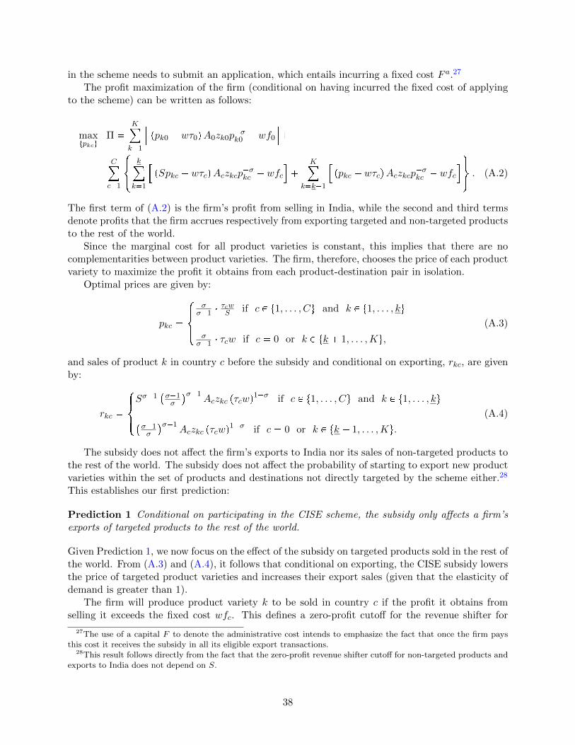
in the scheme needs to submit an application, which entails incurring a fixed cost F a.27

The profit maximization of the firm (conditional on having incurred the fixed cost of applyingto the scheme) can be written as follows:

maxtpkcu

Π �K

k�1

�ppk0 � wτ0qA0zk0p

�σk0 � wf0

��

C

c�1

$&%k

k�1

�pSpkc � wτcqAczkcp

�σkc � wfc

��

K

k�k�1

�ppkc � wτcqAczkcp

�σkc � wfc

�,.- . (A.2)

The first term of (A.2) is the firm’s profit from selling in India, while the second and third termsdenote profits that the firm accrues respectively from exporting targeted and non-targeted productsto the rest of the world.

Since the marginal cost for all product varieties is constant, this implies that there are nocomplementarities between product varieties. The firm, therefore, chooses the price of each productvariety to maximize the profit it obtains from each product-destination pair in isolation.

Optimal prices are given by:

pkc �

$'&'%σσ�1 �

τcwS if c P t1, . . . , Cu and k P t1, . . . , ku

σσ�1 � τcw if c � 0 or k P tk � 1, . . . ,Ku,

(A.3)

and sales of product k in country c before the subsidy and conditional on exporting, rkc, are givenby:

rkc �

$'&'%Sσ�1

�σ�1σ

�σ�1Aczkc pτcwq

1�σ if c P t1, . . . , Cu and k P t1, . . . , ku

�σ�1σ

�σ�1Aczkc pτcwq

1�σ if c � 0 or k P tk � 1, . . . ,Ku.

(A.4)

The subsidy does not affect the firm’s exports to India nor its sales of non-targeted products tothe rest of the world. The subsidy does not affect the probability of starting to export new productvarieties within the set of products and destinations not directly targeted by the scheme either.28

This establishes our first prediction:

Prediction 1 Conditional on participating in the CISE scheme, the subsidy only affects a firm’sexports of targeted products to the rest of the world.

Given Prediction 1, we now focus on the effect of the subsidy on targeted products sold in the rest ofthe world. From (A.3) and (A.4), it follows that conditional on exporting, the CISE subsidy lowersthe price of targeted product varieties and increases their export sales (given that the elasticity ofdemand is greater than 1).

The firm will produce product variety k to be sold in country c if the profit it obtains fromselling it exceeds the fixed cost wfc. This defines a zero-profit cutoff for the revenue shifter for

27The use of a capital F to denote the administrative cost intends to emphasize the fact that once the firm paysthis cost it receives the subsidy in all its eligible export transactions.

28This result follows directly from the fact that the zero-profit revenue shifter cutoff for non-targeted products andexports to India does not depend on S.

38

targeted product-destination combinations given by:

z�kc �pσwqσ

pσ � 1qσ�1�fcAc

��τcS

σ�1. (A.5)

Total exports of eligible product-destination combinations for the firm (conditional on filing forthe subsidy), RE,S , are given by:

RE,S �C

c�1

k

k�1

�» 8z�kc

rkcpzkcqgpzkcqdzkc

�. (A.6)

Firm sales for a given product-destination pair can in turn be decomposed as the product ofthe probability that a firm exports a given product variety, φSkc—the extensive margin—and theaverage export sales per product-destination pair, rSkc—the intensive margin:

RE,S �C

c�1

k

k�1

φSkc � rSkc. (A.7)

The probability that the firm exports targeted product k to country c, φkc, is given by:

φSkc � 1 �G pz�kcq � pz�kcq�a �

pσ � 1qapσ�1q

pσwqσa�

�Acfc

a�

�S

τc

apσ�1q, (A.8)

which is increasing in the subsidy S. Average exports per product-destination, rkc, are given by:

rSkc �1

1 �Gpz�kcq

» 8z�kc

rkcpzkcqgpzkcqdzkc �aσw

a� 1�

�fcAc

, (A.9)

which are independent of the subsidy.Plugging back (A.8) and (A.9) into (A.7) yields:

RE,S � Sapσ�1q �ak

a� 1�pσ � 1qapσ�1q

pσwqσa�1�C

c�1

��fcAc

τσ�1c

�1�a. (A.10)

The expected number of targeted product-destination combinations sold by a firm, NE,Sck , is in

turn given by:

NE,Sck �

1

kC

C

c�1

k

k�1

φkc �1

C�pσ � 1qapσ�1q

pσwqσa� Sapσ�1q

C

c�1

�Ac

fcτ1�σc

a. (A.11)

We now investigate the firm’s decision to participate in the CISE scheme or not. From Prediction1 it follows that a firm would find it profitable to apply to CISE if the increase in operationalprofits of targeted products sold in the rest of the world brought about by the subsidy exceeds theadministrative cost of applying to the scheme, i.e. if

πE,S � πE, S �SRE,S

σ�RE, S

σ¥ wF a, (A.12)

where the first term after the equality denotes after-subsidy operational profits from exporting

39

eligible product-destination combinations, and the second term is the profit that the firm wouldearn if it did not participate in CISE (the term RE, S is identical to equation (A.10) without thesubsidy term in the front).

Using (A.12) we define a cutoff for the gross subsidy, S, such that a firm would choose toparticipate in CISE if the gross subsidy it obtains exceeds this lower bound:

Sapσ�1q�1 � 1 �

�σσa

pσ � 1qapσ�1q

��

�a� 1

ak

��wσaF a

AE, (A.13)

where AE �°Cc�1

�pfc{Acqτ

σ�1c

�1�ais a measure of the effective demand that the firm faces for

eligible products in the rest of the world. It follows directly from (A.13) that the subsidy cutoff islower when AE or k are higher. That is, a firm is more likely to participate in CISE the higher itsbefore-subsidy sales of eligible product-destination combinations are.

Using Equations (A.13), (A.8), (A.9), (A.10) and (A.11), we establish the following predictions:

Prediction 2 An exporter is more likely to participate in the CISE scheme the higher its exportsof targeted products to the rest of the world are before the subsidy is in place.

Prediction 3 Conditional on participating in the CISE scheme, the subsidy increases firms’ ex-ports of targeted products to the rest of the world.

Prediction 4 Conditional on participating in the CISE scheme, the subsidy has a positive effecton the extensive margin of exports of subsidized product-destination pairs. That is, a subsidizedfirm increases the number of targeted products it sells in the rest of the world.

Prediction 5 Conditional on participating in the CISE scheme, the subsidy does not affect averageexports per product-destination—the intensive margin of exports—of targeted products sold in therest of the world.

40

B Matching Diagnostics

Table B.1: Indicators of Matching Quality

Variable Standardized differences Variance ratioRaw Weighted Raw Weighted

IPW PSM NNM IPW PSM NNM

Log export value 1.242 -0.056 -0.009 0.255 0.449 0.852 1.083 1.171Shr. exports to ROW 0.288 0.070 0.006 -0.010 0.441 0.633 0.721 0.789Shr. exports eligible products 0.473 0.050 -0.026 -0.010 0.608 1.155 1.242 0.962Domestic VA ¥ 30% dummy 0.563 -0.032 0.057 0.000 1.692 0.992 1.021 1.000Importer dummy 0.133 0.007 0.000 0.000 0.311 0.928 1.000 1.000Product-level Herfindahl -0.168 -0.01 0.1621 0.063 0.862 1.011 1.947 1.182Physical capital intensity -0.134 0.112 -0.154 0.011 0.425 0.947 0.533 1.001Human capital intensity 0.565 0.001 0.055 0.009 0.958 1.041 1.576 1.024

Imai-Ratkovic overidentification test p-value (H0: covariates are balanced): 0.258

IPW stands for inverse probability weighting, PSM stands for propensity score matching weighting and NNM forMahalanobis matching weighting.

Table B.2: Joint Significance and Pseudo R-squared of Treatment Status Model

Raw data Weighted data

IPW PSM NNM

Pseudo R-squared 0.329 0.004 0.015 0.017χ2 test (p-value) 0.000 0.983 0.745 0.763

The table reports the pseudo R-squared and p-value of the χ2 joint significance test from running the probit modelof the probability of receiving the CISE export subsidy (column (6) of Table 6) and the same statistics when themodel is estimated using only the treated and matched control firms. IPW stands for inverse probability weighting,PSM stands for propensity score matching weighting and NNM for Mahalanobis matching weighting.

41

C Mechanisms

C.1 Effects on Product and Geographic Diversification

Our benchmark specification (estimated at the firm-year level and reproduced in column (1) ofTable C.1 for convenience) shows that subsidized firms significantly increase the number of HS6-digit products they export. Next we aggregate the data at the firm-HS 2-digit product-year leveland estimate an outcome regression similar to (1) in which the dependent variable is the numberof HS 6-digit products that a firm exports within a given HS 2-digit sector. While we still use thesame weighting schemes as in our benchmark regressions, we now include firm, year and HS 2-digitfixed effects.

We follow a similar approach to investigate the extent of geographic diversification engenderedby the CISE subsidy. Column (4) of Table C.1 reproduces our benchmark results (column (2) ofTable 7). Column (5) uses data aggregated at the firm-level and uses the number of continents thata firm exports to—instead of the number of countries as in column (4)—to measure diversification.Column (6) aggregates the data at the firm-continent-year level and uses the number of countriesa firm exports to within a given continent as the dependent variable. This specification includesfirm, year and continent fixed effects.

Table C.1: Extent of Product and Geographic Diversification Effects of the CISE Subsidy

# of Products # of Markets

HS6 HS2 HS6 Countries Continents Countries withinwithin HS2 a continent

(1) (2) (3) (4) (5) (6)

OLS 0.061** 0.025 0.048* 0.086** 0.055** 0.090**(0.030) (0.022) (0.026) (0.033) (0.023) (0.028)

Inverse probability 0.061** 0.024 0.053** 0.108*** 0.065*** 0.109**(IPW) (0.030) (0.024) (0.027) (0.032) (0.024) (0.029)Propensity score 0.077** 0.033 0.061*** 0.119*** 0.069*** 0.117**(PSM) (0.033) (0.025) (0.021) (0.037) (0.025) (0.034)Mahalanobis matching 0.058* 0.013 0.057** 0.093*** 0.058** 0.074*(NNM) (0.033) (0.024) (0.026) (0.035) (0.026) (0.032)

Firm FE Y Y Y Y Y YYear FE Y Y Y Y Y YHS 2-digit FE N N Y N N NContinent FE N N N N N Y

Entries in the table are the average effect of the CISE export subsidy on the log export outcome in the correspondingcolumn among firms that received the subsidy. Standard errors are clustered at the firm-level in parenthesis, exceptin column (2) where two-way clustering is used at the firm and HS 2-digit level and in column (5) where two-wayclustering is used at the firm and continent level. *, **, *** indicate significance at the 10%, 5% and 1% levels,respectively.

42

C.2 Impact on Within-Firm Exit Rate and Sales Dispersion

In the first set of regressions reported in Table C.2 we investigate how the subsidy affects exit at theproduct, destination, product-destination and firm levels. The outcome variable in this analysis isis a dummy that equals one if a firm exported a given product or destination or product-destinationin year t but does not export the same in year t � 1. The outcome variable in the regression incolumn (4) is firm exit—i.e. the dependent variable equals 1 if the firm exports anything in yeart but does not export at all in year t � 1. The data is aggregated at the firm-year level andthe estimating equations are analogous to our benchmark specification: we use different weightingschemes to conduct the matching and both firm and year fixed effects are included.

The dependent variables in the regressions reported in columns (5)-(7) of Table C.2 are respec-tively the standard deviation of the logarithm of firms’ export sales across product-destinations,destinations and products respectively. The estimating equations are analogous to our benchmarkspecification: we use different weighting schemes to conduct the matching and both firm and yearfixed effects are included.

Table C.2: Average Effect of Export Subsidy on CISE Products Sold in the Rest of the World:Impact on Exit and Sales Dispersion

Within-Firm Exit Firm Exit Within-Firm Sales Dispersion

prod.- dest. prod. prod.- dest. prod.dest. dest.(1) (2) (3) (4) (5) (6) (7)

OLS -0.022 -0.025 -0.029 -0.076 -0.056 0.082 -0.140(0.042) (0.045) (0.047) (0.064) (0.068) (0.066) (0.105)

Inverse probability -0.024 -0.040 -0.035 -0.055 0.007 0.128* -0.072(IPW) (0.042) (0.045) (0.048) (0.069) (0.073) (0.071) (0.110)Propensity score -0.028 -0.039 -0.039 -0.080 0.018 0.167** -0.075(PSM) (0.044) (0.046) (0.050) (0.071) (0.077) (0.073) (0.115)Mahalanobis matching -0.037 -0.065 -0.030 -0.057 -0.085 0.040 -0.115(NNM) (0.044) (0.047) (0.052) (0.073) (0.083) (0.078) (0.114)

Entries in the table are the average effect of the CISE export subsidy on the log export outcome at the firm level inthe corresponding column among firms that received the subsidy. All regressions include firm and year fixed effects.Number of products are defined at the number of HS 6-digit level. Standard errors clustered at the firm level inparenthesis. *, **, *** indicate significance at the 10%, 5% and 1% levels, respectively.

43

C.3 Does the Subsidy Encourages More Exports to Countries where TreatedFirms Have Imported From Before?

To answer this question, we identify the countries from which the firms in our data import from in2011. We then run the same weighted outcome regressions as in our benchmark specification for twosub-samples: (i) countries from which firms imported in 2011, and (ii) countries from which theydid not. The objective is to investigate whether the CISE subsidy is more effective in improvingfirms’ export performance in markets in which they had an existing import relationship.

Table C.3: Average Effect of Export Subsidy on CISE Products

Panel A: Sold in Countries (Other than India) from Which Firms have Imported From in 2011

Extensive Margin Intensive Margin Total

Number of import average import sales per importprod.- origin. prod. prod.- origin. prod. valueorigin. origin.

(1) (2) (3) (4) (5) (6) (7)

OLS 0.104** 0.083*** 0.076 -0.058 -0.185 -0.019 0.085(0.050) (0.032) (0.048) (0.139) (0.162) (0.170) (0.145)

Inverse probability 0.125** 0.084** 0.086 0.088 -0.029 0.104 0.253*(IPW) (0.055) (0.033) (0.054) (0.142) (0.164) (0.173) (0.149)Propensity score 0.089 0.063 0.073 0.108 -0.001 0.138 0.216(PSM) (0.061) (0.039) (0.057) (0.173) (0.192) (0.211) (0.184)Mahalanobis matching 0.100 0.056 0.086 0.001 -0.085 0.022 0.130(NNM) (0.061) (0.035) (0.060) (0.137) (0.175) (0.166) (0.150)

Panel B: Sold in Countries (Other than India) From Which Firms have Not Imported From in 2011

Extensive Margin Intensive Margin Total

Number of import average import sales per importprod.- origin. prod. prod.- origin. prod. valueorigin. origin.

(1) (2) (3) (4) (5) (6) (7)

OLS 0.062 0.047 0.062** -0.149* -0.095 -0.100 -0.057(0.039) (0.035) (0.028) (0.090) (0.111) (0.097) (0.097)

Inverse probability 0.077** 0.067* 0.059** 0.027 0.014 0.023 0.122(IPW) (0.039) (0.035) (0.029) (0.097) (0.120) (0.105) (0.102)Propensity score 0.097** 0.088** 0.083*** 0.116 0.068 0.092 0.238*(PSM) (0.043) (0.040) (0.032) (0.131) (0.133) (0.120) (0.139)Mahalanobis matching 0.078* 0.057 0.054* 0.004 0.029 0.033 0.107(NNM) (0.040) (0.037) (0.030) (0.098) (0.122) (0.107) (0.106)

Entries in the tables are the average effect of the CISE export subsidy on the log export outcome at the firm level inthe corresponding column among firms that received the subsidy. All regressions include firm and year fixed effects.Number of products are defined at the number of HS 6-digit level. Standard errors clustered at the firm level inparenthesis. *, **, *** indicate significance at the 10%, 5% and 1% levels, respectively.

44

C.4 Number of Times a Firm Receives the Subsidy

In this section we investigate whether the average treatment effect of the CISE scheme variesaccording to the number of years a firm has received the subsidy over our period of analysis. To doso, we re-estimate our benchmark specification for two sub-samples of exporters: those that receivethe subsidy only once and those that receive it for the three years we observe in our data.

Table C.4: Average Effect of the Export Subsidy —CISE Products Sold in the Rest of the World

Panel A: For Firms Receiving the Subsidy in Only One Year

Extensive Margin Intensive Margin Total

Number of export average sales per exportprod.- dest. prod. prod.- dest. prod. valuedest. dest.(1) (2) (3) (4) (5) (6) (7)

OLS 0.104** 0.117*** 0.084** -0.226** -0.300** -0.244** -0.096(0.046) (0.039) (0.038) (0.109) (0.124) (0.121) (0.115)

Inverse probability 0.133*** 0.145*** 0.085** -0.013 -0.162 -0.094 0.142(IPW) (0.044) (0.038) (0.040) (0.110) (0.126) (0.121) (0.118)Propensity score 0.140*** 0.155*** 0.090** -0.008 -0.155 -0.071 0.162(PSM) (0.050) (0.043) (0.044) (0.121) (0.136) (0.129) (0.129)Mahalanobis matching 0.135*** 0.126*** 0.086** -0.079 -0.173 -0.120 0.089(NNM) (0.046) (0.040) (0.043) (0.117) (0.134) (0.128) (0.125)

Panel B: For Firms Receiving the Subsidy for Three Years

Extensive Margin Intensive Margin Total

Number of export average sales per exportprod.- dest. prod. prod.- dest. prod. valuedest. dest.(1) (2) (3) (4) (5) (6) (7)

OLS 0.270** 0.240** 0.142*** -0.408* -0.581 -0.189 0.049(0.133) (0.112) (0.050) (0.234) (0.548) (0.314) (0.182)

Inverse probability 0.336** 0.287** 0.191*** -0.028 -0.362 0.010 0.499**(IPW) (0.135) (0.114) (0.054) (0.248) (0.553) (0.321) (0.201)Propensity score 0.392*** 0.302** 0.228*** 0.027 -0.341 0.006 0.634**(PSM) (0.143) (0.121) (0.064) (0.292) (0.582) (0.365) (0.251)Mahalanobis matching 0.360** 0.264** 0.177*** -0.141 -0.434 -0.050 0.435**(NNM) (0.145) (0.123) (0.064) (0.250) (0.567) (0.332) (0.205)

Entries in the tables are the average effect of the CISE export subsidy on the log export outcome in the correspondingcolumn among firms that received the subsidy. All regressions include firm and year fixed effects. Products are definedat the HS 6-digit level. Standard errors clustered at the firm level in parenthesis. *, **, *** indicate significance atthe 10%, 5% and 1% levels, respectively.

45

C.5 Has CISE Encouraged Export Round Tripping?

In this set of regressions we investigate whether subsidized exporters also increase their imports ofproducts included in the CISE scheme. The idea is that if the cost of exporting and re-importinga product to the rest of the world is lower than the additional profit that a firm accrues from thesubsidy, the CISE scheme could in fact be subsidizing domestic sales.

Table C.5: Average Effect of Export Subsidy on Imports of CISE products from the Rest of theWorld

Extensive Margin Intensive Margin Total

Number of import average import sales per importprod.- origin. prod. prod.- origin. prod. valueorigin. origin.

(1) (2) (3) (4) (5) (6) (7)

OLS 0.073 0.026 0.125 0.415 0.280 0.175 0.488(0.102) (0.058) (0.104) (0.256) (0.235) (0.229) (0.299)

Inverse probability 0.072 0.071 0.123 0.400 0.308 0.235 0.473(IPW) (0.111) (0.063) (0.112) (0.287) (0.262) (0.255) (0.330)Propensity score 0.065 0.083 0.106 0.262 0.196 0.168 0.329(PSM) (0.119) (0.068) (0.119) (0.304) (0.275) (0.269) (0.344)Mahalanobis matching 0.188 0.083 0.224 0.168 0.074 -0.032 0.361(NNM) (0.176) (0.063) (0.177) (0.323) (0.302) (0.306) (0.375)

Entries in the table are the average effect of the CISE export subsidy on the log import outcome at the firm level inthe corresponding column among firms that received the subsidy. All regressions include firm and year fixed effects.Number of products are defined at the number of HS 6-digit level. Standard errors clustered at the firm level inparenthesis. *, **, *** indicate significance at the 10%, 5% and 1% levels, respectively.

46

D Sectoral Heterogeneity

D.1 HS 2-digit Product Fixed-Effects and Two-way Clustering of StandardErrors

We aggregate the data at the firm-HS 2-digit product-year level and estimate our outcome re-gressions using the same weighting schemes as in our benchmark to implement the matching. Weinclude firm, HS 2-digit and year fixed effects and cluster standard errors at the firm and HS 2-digitproduct level.

Table D.1: Average Effect of Export Subsidy at the firm-HS 2-digit product level—CISE Productssold in the Rest of the World

Extensive Margin Intensive Margin Total

Number of export average sales per exportprod.- dest. prod. prod.- dest. prod. valuedest. dest.(1) (2) (3) (4) (5) (6) (7)

OLS 0.092*** 0.082*** 0.048* -0.130** -0.107* 0.000 0.143*(0.025) (0.017) (0.026) (0.058) (0.054) (0.076) (0.078)

Inverse probability 0.100*** 0.093*** 0.053** 0.061 -0.041 0.073 0.230***(IPW) (0.025) (0.016) (0.027) (0.064) (0.073) (0.091) (0.084)Propensity score 0.108*** 0.093*** 0.061*** 0.058 -0.005 0.049 0.213***(PSM) (0.017) (0.010) (0.021) (0.065) (0.082) (0.074) (0.071)Mahalanobis matching 0.107*** 0.087*** 0.057** -0.053 -0.070 0.025 0.182**(NNM) (0.020) (0.008) (0.026) (0.070) (0.069) (0.090) (0.073)

Firm FE Y Y Y Y Y Y YYear FE Y Y Y Y Y Y YHS 2-digit FE Y Y Y Y Y Y Y

Entries in the table are the average effect of the CISE export subsidy on the log export outcome at the firm-HS2-digit product level in the corresponding column among firms that received the subsidy. All regressions include firm,HS-2 digit product and year fixed effects. Number of products exported are defined at the HS 6-digit level. Standarderrors clustered at the firm and HS 2-digit product levels in parenthesis. *, **, *** indicate significance at the 10%,5% and 1% levels, respectively.

47

D.2 Textiles and Clothing Products and Agricultural Products

We split our data across two very broad sectors: clothing and textiles (HS 2-digit sectors 50 to63) and agricultural products (HS 2-digit sectors 00 to 24). Agricultural products encompass thegoods classified as ‘agricultural’ in the policy (see column 3 of Table 1) in addition to other productssuch as coffee, tea, honey, flour, etc. that fall under the ‘industrial products’ of CISE (columns1 and 2 of Table 1). For each broad sector we separately estimate a probit model like the onereported in column (6) of Table 6 and outcome regressions using the same weighting schemes as inour benchmark specification. Thus the counterfactuals for subsidized firms are now restricted tobelong to the same sector.

Table D.2: Average Effect of the Export Subsidy— CISE Products Sold in the Rest of the World

Panel A: Textiles and Clothing Products

Extensive Margin Intensive Margin Total

Number of export average sales per exportprod.- dest. prod. prod.- dest. prod. valuedest. dest.(1) (2) (3) (4) (5) (6) (7)

OLS 0.081* 0.071** 0.085** -0.118 -0.143 -0.119 -0.011(0.042) (0.032) (0.038) (0.093) (0.105) (0.102) (0.110)

Inverse probability 0.107*** 0.073** 0.109*** 0.042 -0.020 0.018 0.169(IPW) (0.040) (0.032) (0.037) (0.093) (0.107) (0.101) (0.108)Propensity score 0.110** 0.078** 0.101** 0.032 -0.037 -0.019 0.159(PSM) (0.045) (0.034) (0.042) (0.100) (0.118) (0.107) (0.116)Mahalanobis matching 0.112** 0.080** 0.100** 0.075 0.018 0.034 0.217*(NNM) (0.044) (0.035) (0.039) (0.101) (0.117) (0.113) (0.119)

Panel B: Agricultural Products

Extensive Margin Intensive Margin Total

Number of export average sales per exportprod.- dest. prod. prod.- dest. prod. valuedest. dest.(1) (2) (3) (4) (5) (6) (7)

OLS 0.024 -0.003 0.076 -0.362 -0.394 -0.405 -0.194(0.062) (0.050) (0.055) (0.227) (0.240) (0.301) (0.254)

Inverse probability 0.071 0.047 0.074 0.107 0.083 0.065 0.308(IPW) (0.063) (0.054) (0.060) (0.388) (0.394) (0.424) (0.388)Propensity score 0.076 0.05 0.043 0.075 0.069 -0.144 0.308(PSM) (0.067) (0.059) (0.057) (0.525) (0.528) (0.642) (0.494)Mahalanobis matching 0.019 -0.013 0.047 0.505 0.488 0.462 0.625(NNM) (0.062) (0.046) (0.058) (0.470) (0.480) (0.507) (0.471)

Entries in the tables are the average effect of the CISE export subsidy on the log export outcome in the correspondingcolumn among firms that received the subsidy. All regressions include firm and year fixed effects. Products are definedat the HS 6-digit level. Standard errors clustered at the firm level in parenthesis. *, **, *** indicate significance atthe 10%, 5% and 1% levels, respectively.

48

CENTRE FOR ECONOMIC PERFORMANCE

Recent Discussion Papers

1691 Adam Altmejd

Andrés Barrios-Fernández

Marin Drlje

Joshua Goodman

Michael Hurwitz

Dejan Kovac

Christine Mulhern

Christopher Neilson

Jonathan Smith

O Brother, Where Start Thou? Sibling

Spillovers on College and Major Choice in

Four Countries

1690 Michael Amior

Alan Manning

Monopsony and the Wage Effects of

Migration

1689 Frank Pisch Managing Global Production: Theory and

Evidence from Just-in-Time Supply Chains

1688 Barbara Petrongolo

Maddalena Ronchi

A Survey of Gender Gaps through the Lens of

the Industry Structure and Local Labor

Markets

1687 Nick Jacob

Giordano Mion

On the Productivity Advantage of Cities

1686 Andrew E. Clark

Anthony Lepinteur

A Natural Experiment on Job Insecurity and

Fertility in France

1685 Richard Disney

John Gathergood

Stephen Machin

Matteo Sandi

Does Homeownership Reduce Crime? A

Radical Housing Reform in Britain

1684 Philippe Aghion

Roland Bénabou

Ralf Martin

Alexandra Roulet

Environmental Preferences and Technological

Choices: Is Market Competition Clean or

Dirty?

1683 Georg Graetz Labor Demand in the Past, Present and Future

1682 Rita Cappariello

Sebastian Franco-Bedoya

Vanessa Gunnella

Gianmarco Ottaviano

Rising Protectionism and Global Value

Chains: Quantifying the General Equilibrium

Effects

1681 Felipe Carozzi

Christian Hilber

Xiaolun Yu

On the Economic Impacts of Mortgage Credit

Expansion Policies: Evidence from Help to

Buy

1680 Paul Frijters

Christian Krekel

Aydogan Ulker

Machiavelli Versus Concave Utility

Functions: Should Bads Be Spread Out Or

Concentrated?

1679 Antoine Dechezleprêtre

David Hémous

Morten Olsen

Carlo Zanella

Automating Labor: Evidence from Firm-Level

Patent Data

1678 Michael Amiior The Contribution of Immigration to Local

Labor Market Adjustment

1677 Swati Dhingra

Silvana Tenreyro

The Rise of Agribusiness and the

Distributional Consequences of Policies on

Intermediated Trade

1676 Jeffrey Grogger

Ria Ivandic

Tom Kirchmaier

Comparing Conventional and Machine-

Learning Approaches to Risk Assessment in

Domestic Abuse Cases

1675 Mary Amiti

Stephen J. Redding

David E. Weinstein

Who’s Paying for the U.S. Tariffs? A Longer-

Term Perspective

1674 Cheng Chen

Claudia Steinwender

Import Competition, Heterogeneous

Preferences of Managers and Productivity

The Centre for Economic Performance Publications Unit

Tel: +44 (0)20 7955 7673 Email info@cep.lse.ac.uk

Website: http://cep.lse.ac.uk Twitter: @CEP_LSE