ISSN 2042-2695

CEP Discussion Paper No 1609

March 2019

Childhood Circumstances and Young Adult Outcomes: The Role of Mothers’ Financial Problems

Andrew E. Clark Conchita D’Ambrosio

Marta Barazzetta

Abstract We here consider the cognitive and non-cognitive consequences on young adults of growing up with a mother who reported experiencing major financial problems. We use UK data from the Avon Longitudinal Study of Parents and Children to show that early childhood financial problems are associated with worse adolescent cognitive and non-cognitive outcomes, controlling for both income and a set of standard variables, and in value-added models controlling for children’s earlier age-5 outcomes. The estimated effect of financial problems is almost always larger in size than that of income. Around one-quarter to one-half of the effect of financial problems on the non-cognitive outcomes seems to transit through mother’s mental health. Key words: income, financial problems, child outcomes, subjective well-being, behaviour, education, ALSPAC JEL Codes: I31; I32; D60 This paper was produced as part of the Centre’s Wellbeing Programme. The Centre for Economic Performance is financed by the Economic and Social Research Council. We are grateful to Liyousew Borga, Martin Evans, Maya Gold, Paul Gregg, Anthony Heyes, David Johnson, Ariel Kalil, Richard Layard, Federico Perali, Mark Stabile, Michael Wolfson, Frances Woolley and all of the members of the well-being group at the LSE for useful comments and valuable suggestions. We also thank seminar participants at Aachen, Basel, the CEP Away Day, CERGE Prague, Duisburg-Essen, the EALE Conference (Ghent), East London, the ECINEQ Conference (Luxembourg), the HEIRS Conference (Lugano), the IARIW Conference (Dresden), the Inequality and Inclusive Growth conference (Chengdu), ISER, Kent Business School, Kings College London, Kingston, Korea Labor Institute, the LABEX OSE Rencontres d’Aussois, Leeds, LSE, LUMSA, the Luxembourg-Singapore Well-Being Workshop, Maastricht, National University of Singapore, Orléans, Ottawa, Örebro, the Paris Seminar in Demographic Economics, the PEARL Workshop (Luxembourg), PSE, Regensburg, Salerno, the 23rd SIEP Conference (Lecce), Stockholm (SOFI), Trier, UCL, University of East Anglia, the World Bank and Xi'an Jiaotong University. We are extremely grateful to all the families who took part in this study, the midwives for their help in recruiting them, and the whole ALSPAC team, which includes interviewers, computer and laboratory technicians, clerical workers, research scientists, volunteers, managers, receptionists and nurses. The UK Medical Research Council and the Wellcome Trust (Grant ref: 102215/2/13/2) and the University of Bristol provide core support for ALSPAC. This work was also supported by the French National Research Agency, through the program Investissements d'Avenir, ANR-10-LABX-93-01. Andrew Clark is grateful for support from CEPREMAP, the US National Institute on Aging (Grant R01AG040640), the John Templeton Foundation and the What Works Centre for Wellbeing. Marta Barazzetta and Conchita D'Ambrosio also thank the Fonds National de la Recherche Luxembourg for financial support. Andrew E. Clark, Paris School of Economics and Centre for Economic Performance, London School of Economics. Conchita D’Ambrosio, Université du Luxembourg. Marta Barazzetta, Université du Luxembourg. Published by Centre for Economic Performance London School of Economics and Political Science Houghton Street London WC2A 2AE All rights reserved. No part of this publication may be reproduced, stored in a retrieval system or transmitted in any form or by any means without the prior permission in writing of the publisher nor be issued to the public or circulated in any form other than that in which it is published. Requests for permission to reproduce any article or part of the Working Paper should be sent to the editor at the above address. A.E Clark, C. D’Ambrosio and M. Barazzetta, submitted 2019.

2

1. Introduction

The Great Recession of 2008-2009 and EU sovereign-debt crisis of 2011-2013 put many

European families at risk of poverty, material deprivation and social exclusion, worsening their

material conditions and overall standard of living. One particular feature of this double-dip

downturn is that it affected not only the poorest but rather a broad swathe of the population that

has not fully recovered. The Quarterly Review on the employment and social situation published

by the European Commission in February 2018 shows that the number of families who experienced

financial distress, there defined as the need to draw on savings or run into debt to cover current

expenditure, remains high. The European financial-distress figure is currently about 14% of the

population, a figure far above that of a decade earlier, and has receded only gradually from 17%,

its highest value at the end of 2013 (the last year of the sovereign-debt crisis). This rise in financial

distress came about not only in the bottom quartile of the income distribution, but also in the 2nd

and 3rd quartiles, namely the wider middle-class. As such, it is commonly-believed that economic

instability affects a great many people’s lives.

There is a very large literature on the relationship between income and financial resources,

on the one hand, and adult outcomes on the other. This has considered the impact of job loss, health

shocks, inheritances, lottery wins and tax refunds, amongst other events. A smaller but still

considerable set of contributions has focussed on potential effects on the children of the adults

concerned. These have considered the intergenerational effect of parental job loss (Hilger, 2016,

Oreopoulos et al., 2008, Rege et al., 2011, and Stevens and Schaller, 2011), parental income (Akee

et al., 2010, Bastian and Michelmore, 2018, Dahl and Lochner, 2012, and Hoynes et al., 2016;

Duncan et al., 2017, provide a meta-analysis) and parental health shocks (Persson and Rossin-

Slater, 2018, and Matsumoto, 2018).

Our contribution is also in the realm of intergenerational correlations. The broad question we

ask is whether income is a sufficient statistic to reflect parental financial difficulties and, if not,

how we can improve the analysis to better study intergenerational transmissions. In general, we

need to know both financial resources and the demands that are made upon them in order to say

whether individuals are in financial distress. As such, indicators of difficulty paying bills or having

had financial problems may provide information over and above the income that individuals or

households receive. We here ask whether the trace of parental financial problems, conditional on

3

parental income, can be found in the adolescent cognitive and non-cognitive outcomes of their

children. This kind of transmission has been suggested in work on the Great Depression of the

1930s (Elder, 1999). For the Commission on the Measurement of Economic Performance and

Social Progress (see Stiglitz et al., 2009, p.198) “This insecurity may generate stress and anxiety

in the people concerned, and make it harder for families to invest in education and housing.” We

are interested in children’s adolescent cognitive and non-cognitive outcomes both in their own right

as measures of how well young people are doing, and because they predict outcomes throughout

adult life.1

One well-known contribution underlining the importance of financial distress is the executive

summary of the Shriver Report: A Woman’s Nation Pushes Back from the Brink (2014), written by

Maria Shriver and the Center for American Progress. This report includes contributions from

Beyoncé, Hillary Clinton and Eva Longoria, among others, and aims to convey the national crisis

from women’s point of view, in an era in which women constitute half of the American labour

force and two-thirds of the primary or co-breadwinners in families.2 This summary opens with a

statement claiming that the most common shared story in today’s America is family financial

insecurity caused by financial problems. One in three women face financial difficulties: “Forty-

two million women, and the 28 million children who depend on them, are living one single

incident—a doctor’s bill, a late paycheck, or a broken-down car—away from economic ruin.

Women make up nearly two-thirds of minimum-wage workers, the vast majority of whom receive

no paid sick days. This is at a time when women earn most of the college and advanced degrees in

this country, make most of the consumer spending decisions by far, and are more than half of the

nation’s voters.” The report describes these women facing financial insecurity, and proposes

policies to improve their quality of life.

We here use data from the Avon Longitudinal Study of Parents and Children (ALSPAC) in

the UK and take a wider view of economic resources to include both income (as in much of the

existing work) and financial distress. This large-scale birth-cohort data follows children over a

period of more than two decades. For each of the child’s first 11 years we know whether the mother

1 Childhood emotional health is the most important predictor of life satisfaction at all adult ages in both the British

Cohort Study (BCS) and the National Child Development Study (NCDS): see Clark et al. (2018), Layard et al. (2014)

and Flèche et al. (2019). 2 The US is no exception in this respect: 46.1 percent of those in work in the EU in 2018 were women, nearly 60

percent of EU university graduates are women and a majority of women with children (61 percent) are also

breadwinners or co-breadwinners.

4

had a major financial problem the previous year. This self-reported variable may be a better

indicator of financial insecurity, and thus parental stress, than income on its own: this is the

conclusion of a number of contributions in the developmental psychology literature (see Kalil,

2013, among many others, for an excellent survey).

The addition of financial distress will not advance our knowledge much if it this almost

entirely determined by income. But if the former reflects both economic resources and the demands

that are made on them, income on its own may tell only half of the story. Financial insecurity does

not necessarily imply low or lower income (and we indeed only find a quite small correlation

between financial problems and income in the ALSPAC data), but includes “a doctor’s bill, a late

paycheck, or a broken-down car”, housing problems, the job loss of a family member, divorce,

falling housing equity, and so on. During the recent Great Recession, these financial problems have

arguably become more widespread than low income, and have hit the middle-class as well (as

highlighted, for example, by Gauthier and Furstenberg, 2010, in relation to families with children).

Some supportive evidence on this point comes from Waves 1 to 18 (1991-2008) of the British

Household Panel Survey (BHPS) data, the dataset often used to analyse income dynamics in the

UK. In the BHPS individuals are asked “Would you say that you yourself are better off or worse

off financially than you were a year ago?”. Around one quarter say better-off, one quarter worse-

off and almost exactly one half about the same. Starting in Wave 3 of the BHPS, respondents who

reported being better or worse off were asked “Why is that?”, with the answers to this open-ended

question being reported verbatim.3 Three response categories dominate for those whose financial

position has worsened: a rise in expenses for almost exactly 50% of respondents, followed by a fall

in income (28%) and “Other” (11%). None of the 18 other reasons that are coded are cited by more

than 4% of respondents whose financial situation worsened. These figures are very similar for those

who have children in the household, and for those who have children under age 12 in the household

(at 47%, 33% and 12% respectively). Financial problems are thus more often caused by increased

expenses than by lower income.

Our analysis of mother’s major financial problems shows that these are associated with worse

cognitive and non-cognitive outcomes of their children up to 18 years later. This correlation persists

when controlling for average family income during childhood, home-ownership, the number of

3 See the BHPS questionnaire. For example, this is question F6 in Wave 18:

https://www.iser.essex.ac.uk/bhps/documentation/pdf_versions/survey_docs/wave18/index.html.

5

years of falls in income that the mother reports and a set of standard variables (and is larger than

the correlation between the child outcomes and income). Major financial problems in early (ages

0 to 5) and later (ages 6 to 11) childhood have broadly similar correlations with most of the

adolescent outcomes. Last, the size of the correlation between financial problems and later

adolescent outcomes continues when we control for child outcomes at around age 5, and only

consider financial problems that appear between the ages of 6 and 11 in a value-added analysis.

These findings suggest that economic downturns, such as the recent Great Recession, and the

financial distress they engender not only affect the adults concerned, but also cast a long shadow

over their children’s outcomes for many decades.

The remainder of the paper is organised as follows. Section 2 contains a short review of the

relevant literature; the dataset, variables and empirical methods are then described in Section 3.

The main results and a series of extensions appear in Section 4. Last, Section 5 concludes.

2. Existing Literature

Research across a variety of disciplines has considered the relationship between the

sufficiency of financial resources and family background on the one hand and later-life child

outcomes on the other. Two broad channels have been examined. In the first resource or investment

channel, income directly acts on the family’s ability to obtain the resources and services required

for child development; in the second family-process channel, the effect of economic resources

works via family relationships and parents’ behaviour towards their children by reducing parental

stress. Haveman and Wolfe (1995) provide an excellent summary of the research across the

disciplines in this context.

In the (direct) resource channel the family is an economic unit deciding how best to allocate

its resources (Becker, 1981, Becker and Tomes, 1986 and 1994). The amount, type and timing of

the resources allocated to children directly influence their future achievements. This is a choice-

based view of children’s attainments, depending on the choices made by society (policy

instruments), parents (the resource channel), and the children themselves (for example in terms of

their own behaviour and effort).

Other disciplines, in particular developmental psychology, have emphasised the relevance of

the indirect effect via the family-process channel (Conger et al., 2010, Voydanoff, 1990): economic

problems may produce worse marital and parent-child relationships, increase household conflict,

and reduce the time and quality of time spent in activities with the child. In addition, parents are

6

role models for their children, and parental behaviour, attitudes and well-being affect the child’s

cognitive and behavioural development. As such, stressful events during childhood can create

emotional distress that undermines child development (McLoyd, 1990 and 1998).

The empirical literature can also be split into that regarding the direct effect of income on

children’s achievements (see, for example, Blau, 1999, Shea, 2000, Maurin, 2002, Hardy, 2014,,

Akee et al., 2018), and that on the indirect effect (Guo and Harris, 2000, Yeung et al., 2002, Conger

et al., 2010,Washbrook et al., 2014). The overall conclusion here is that income does matter for

child outcomes. There is more evidence for cognitive outcomes than for non-cognitive outcomes,

as the latter have rarely if at all been explored using large-scale cohort data (for reviews see Mayer,

1997, Duncan and Brooks-Gunn, 1997, Haveman and Wolfe, 1995, Conger et al., 2010). We

discuss some of this relevant literature below.

2.1 Cognitive Outcomes

Blanden and Gregg (2004) analyse three British datasets, and conclude that a one-third

reduction in family income leads to an average 3-4 percentage-point fall in the probability of

achieving GSCE A-C grades or obtaining a degree. Ermisch and Francesconi (2001) consider

various family characteristics in the first seven waves of the BHPS, and conclude that income is a

strong predictor of educational attainment. Gregg and Machin (2000) estimate the effects of family

background on children’s educational attainment and labour-market outcomes at ages 16, 23 and

33 using British NCDS data. The strongest negative family-related predictor of school attendance

and staying on at school at age 16 is financial hardship (defined as whether the family experienced

financial difficulties in the year prior to the survey date). Children in families experiencing

financial difficulties were also more likely to have contact with the police and experience

unemployment at age 23, and earn lower wages at age 33. Maurin (2002) uses French INSEE data

to show that ten percent higher family income is associated with a 6.5 percentage-point lower

probability of being held back a year in elementary school. In Acemoglu and Pischke (2001), 10

percent higher family income leads to about 1.4 percentage point rise in the probability of child

college attendance.

Other work, mainly on US data, has uncovered smaller income effects. Blau (1999), for

example, finds a small, and in some cases insignificant, effect of current income on children’s

outcomes in National Longitudinal Survey of Youth (NLSY) data. The effect of permanent income

is larger than that of transitory income, but still smaller than that of other family characteristics

7

such as mother’s ability or ethnicity. Hardy (2014) presents evidence from the Panel Study of

Income Dynamics (PSID) that family-income volatility has a negative effect on post-secondary

education but no effect on adult income.

Some work has used non-income measures of economic resources: wealth or financial assets

reflect financial security that can reduce family stress and financial anxiety and promote child

development. Yeung and Conley (2008) look at family wealth and Black-White test-score gaps in

children aged 3 and 12 in PSID data. Wealth plays no role for the test-score gaps of pre-school

children but does so for in-school children; wealth is also shown to be significantly correlated with

mediating factors such as parental warmth, parental activities with the child, and the learning

resources available at home. Kim and Sherraden (2011) analyse the effect of financial assets, non-

financial assets, and home ownership on high-school completion and college-degree attainment.

Assets significantly predict children’s educational outcomes, reduce the size of the income effect

and, in some cases, even render it insignificant.

The indirect effect of family income on child development includes parental behaviour

toward the child, family relationships, the home environment, stimulating material at home, and

activities. Washbrook et al. (2014) use the same ALSPAC data as we do here and find both direct

and indirect effects of family income on the cognitive outcomes of children aged between 7 and 9,

but not on their non-cognitive outcomes. Yeung et al. (2002) uncover both direct and indirect

income effects on child cognitive outcomes at ages 3 through 5 in PSID data, with the direct effect

being reduced by the introduction of the indirect effects. Yeung et al. also look at economic

instability, measured by a year-on-year fall in income of at least 30 percent. This has a direct effect

on some test scores, a small effect on behavioural problems, but a larger effect on mediating factors

such as mother’s mental well-being and parental behaviour, which in turn significantly affect child

development. We will address the question of income falls in Section 4 below.

2.2 Non-cognitive Outcomes

Duncan and Brooks-Gunn (1997) suggest that non-cognitive outcomes are in general less

sensitive to family income than are cognitive outcomes. Some work has found a positive correlation

between income and children’s physical health (see, among others, Case and Paxson, 2002, for the

US, and Currie and Stabile, 2003, for Canada). However, there is no link between low-income and

health in ALSPAC data in Propper et al. (2007) once mother’s health, including mental health, has

been controlled for.

8

Children from low-income families appear to have more psychological and behavioural

problems (McLeod and Shanahan, 1993, and Bolger et al., 1995), with the effect working only

indirectly via family stress and parental attitudes towards the child (see, among others, Yeung et

al., 2002, for the US, and Washbrook et al., 2014, for the UK), with no direct income effect.

Analogously, child emotional well-being and mental health seem to be affected by family income

only indirectly via its effect on family stress (see, for example, Mistry et al., 2002). Income and

child self-esteem do not seem to be correlated (Axinn et al., 1997, and Washbrook et al., 2014),

although the importance of timing in children’s non-cognitive outcomes, and in particular

children’s mental health in adulthood, remains to be established. Sobolewski and Amato (2005)

report that economic hardship, such as family income, the value of equity in the family home and

the value of other financial assets, has long-term consequences for adult psychological well-being,

such as self-esteem, distress symptoms, and satisfaction in various life domains. Their findings are

based on a small US sample of 589 observations from the Martial Instability Over the Life Course

Study. As above, the effect runs indirectly via parents’ financial stress. Similarly, Wickrama et al.

(2005) use data on 451 Iowa families to show that family income directly influences adolescent

mental disorder and physical illness, and Evans and Cassells (2014) find that greater poverty

exposure in the first nine years is associated with worse mental health outcomes in the later teens,

using a sample of 196 families in upstate New York. However, there is no relationship between

family income and child psychiatric disorder in the British Child and Adolescent Mental Health

Survey (Ford et al., 2004).

We will here add to this existing literature by providing systematic evidence from a large-

scale long-run birth cohort survey. We consider not only cognitive, but also health, behaviour and

subjective well-being outcomes. These latter are reported not only by the carer, but also by the

children themselves and sometimes by the child’s teacher (the cognitive outcomes are matched in

from the national exam results database). We relate these outcomes to family income, as in most

of the existing literature, and, more originally, to household financial problems as reported by the

child’s mother over an eleven-year period. Our broad conclusion is that income on its own is an

insufficient statistic for family economic resources and the demands that are made on them:

conditional on income and home ownership, the incidence of financial problems is a significant

predictor of almost all of our adolescent-outcome measures, and with an effect size that is typically

much larger than that of income.

9

3. Data and Methods

The ALSPAC survey, also known as “The Children of the 90s”, is a long-term health research

project that recruited over 14,000 pregnant women who were due to give birth between April 1991

and December 1992 in Bristol and its surrounding areas, including some of Somerset and

Gloucestershire. These women and their families have been followed ever since, even if they move

out of the original catchment area (See http:// www.bristol.ac.uk/alspac/).

The initial sample was composed of 14,541 pregnant women who enrolled in the ALSPAC

study, resulting in a total of 14,062 live births of whom 13,988 were alive at the age of one year.

Although the ALSPAC sample in Avon is richer and Whiter than the UK on average, the children

are very similar to the UK average in terms of height and weight at birth, and at ages one and two

years (see http://ije.oxfordjournals.org/content/early/2012/04/14/ije.dys064.full.pdf for a full

description of the cohort profile). The study website contains a fully searchable data dictionary of

all of the data that is available (http://www.bris.ac.uk/alspac/researchers/data-access/data-

dictionary/). Ethical approval for the study was obtained from the ALSPAC Ethics and Law

Committee and the Local Research Ethics Committee.

3.1 Dependent Variables

We consider five types of child outcome during adolescence/early adulthood: subjective

well-being (henceforth SWB), behaviour, emotional health, physical health and education.

Child SWB is measured via the Short Moods and Feelings Questionnaire (SMFQ), which is

composed of a number of items reflecting how the child felt over the past two weeks, such as being

miserable or unhappy, crying a lot, and feeling lonely: see Appendix B2 for the questionnaire. Each

item is answered on a three-point scale (true (0), sometimes true (1), and not true (2)).The SMFQ

is child-reported at ages 16 and 18, and carer-reported (most often the mother) at age 16. It consists

of 17 items for the child-reported version at age 16 and 13 items for the other two versions. To

make the results comparable over time, we use the 13 items that are common to both ages. The

total SMFQ score, the sum of the answers to these 13 questions, ranges between 0 and 26, with

higher numbers indicating better SWB.

Child antisocial behaviour at ages 11 and 16 is measured by the Troublesome Behaviours

Score from the Development and Well-Being Assessment (DAWBA) questionnaire. The DAWBA

is a long questionnaire assessing common emotional, behavioural and hyperactivity disorders

among children aged 5 to 17 (it is not designed to assess severe disorders), and can be administrated

10

to children, teachers or the carer. It consists of several sections, each assessing a different type of

child disorder (e.g. depression, hyperactivity, phobias, and self-harm). The troublesome behaviours

section asks the carer and the teacher if over the last 12 months (over the past school year in the

teacher’s version) the child had exhibited a number of different behaviours. The carer-and teacher-

reported versions of the questionnaire are slightly different, with the carer-reported questionnaire

consisting of a list of 15 behaviours,4 with possible answers of “No”, “Perhaps” and “Definitely”

(coded 0, 1 and 2) for seven minor troublesome behaviours, and “Yes” or “No” (coded 1 or 0) for

eight more serious behaviours), and the teacher-reported version of 12 behaviours, with possible

answers of “Not true”, “Somewhat true”, “Certainly true” (coded 0, 1 and 2). These behaviours

include bullying people, fighting with other siblings, stealing from shops, and hurting or being

physically cruel with someone. Despite the different number of questions, the total antisocial

behaviour score in both versions ranges from 0 to 22, with higher scores indicating worse behaviour

(see Appendices B3 and B4). In ALSPAC the DAWBA questionnaire is administered to teachers

when the child is aged 11 and to carers when the child is aged 16.

Both child emotional health and a second measure of behaviour come from the Strengths and

Difficulties Questionnaire (henceforth SDQ). The SDQ is a behavioural-screening questionnaire

for children about 3 to 16 years old and consists of 25 questions that are answered by an adult

regarding the child’s concentration span, temper tantrums, happiness, worries and fears, whether

the child is obedient, often lies or cheats, and so on: see Appendix B5. The answers to these

questions can be used to produce five well-being sub-scales (each consisting of five items) referring

to emotional health, behavioural problems, hyperactivity/inattention, peer-relationship problems,

and pro-social behaviour. Following Goodman et al. (2010), we use two broader sub-scales, as in

low-risk samples such as the ALSPAC respondents the five finer sub-scales may not be able to

detect distinct aspects of child well-being. The “internalising behaviour” score is the sum of the

emotional and peer subscales, and can be argued to measure emotional health, while “externalising

behaviour” is made up of the behavioural problems and hyperactivity subscales and refers to

behaviour. Both internalising and externalising SDQ are scored on a 0-20 scale; we reverse this

scale so that higher values indicate better outcomes. We have both carer- and teacher-reported SDQ

at age 11.

4 The original list includes also “forcing someone into sexual activity against their will” among the possible antisocial

behaviours: as this item resulted in zero affirmative cases we exclude it from the list.

11

Children’s physical health is measured by their BMI at ages 11, 13 and 16, compared to the

distribution of BMI in other children of the same age by sex (calculated from within the ALSPAC

survey). This measure is based on clinically-assessed height and weight. We construct a dummy

variable for having “normal” BMI between the 5th and 85th percentiles. We will below consider

some alternative child-health measures.

Last, our cognitive outcomes refer to the results of the GCSE qualifications or equivalent

exams (Key Stage 4, or KS4), taken in the UK at the end of compulsory schooling (at age 16),

matched in from the National Pupil Database.5 The lowest GCSE exam grade of G is assigned 16

points, and the points for successive grades rise in steps of 6 up to the top grade of A* with 58

points.6 At the pupil-level, KS4 outcomes are given in five mutually-exclusive groups: level 2 (five

or more A*-C GCSEs or equivalent); level 1 (five or more A*-G GCSEs or equivalent); one or

more level-1 standard qualifications (1 or more A*-G GCSEs or equivalent, but not five or more);

only entry-level qualifications (GCSEs with grades below G); and no passes. We consider a dummy

for achieving the highest level (level 2), and average GCSE points (total exam points divided by

the total number of entries).

The summary statistics for all of the different child-outcome variables are presented in

Appendix Table A1.

3.2 Explanatory Variables

We wish to relate the above dependent variables to the financial resources that were available

to the household when the child was growing up. Household income is measured in ALSPAC when

the child is aged 3, 4, 7, 8, and 11. The question “On average, about how much is the take home

family income each week (include social benefits etc.)?”is answered using a scale of five income

bands at ages 3, 4, 7 and 8, and ten income bands at age 11. We convert these ALSPAC band values

at each wave to income figures using data from the Family Resources Survey (FRS) on the

distribution of net household income in the South West region, deflated to 2008 prices. We are

careful to match this distribution by year of birth (for 1991 births at age 3, we use the 1994 income

5 The National Pupil Database (NPD) contains information on pupils’ educational attainments in England, including

test and exam results at different key stages. To date, information on key-stage results is available for each ALSPAC

study child at ages 7, 11, 14 and 16. The definition of the different key stages can be found at

https://www.gov.uk/national-curriculum/overview. 6https://www.gov.uk/government/uploads/system/uploads/attachment_data/file/517106/Key_stage_4_average_grade

_per_qualification_2015.pdf.

12

distribution, but the 1995 income distribution for 1992 births, and so on). The original income

bands and the resulting FRS net household income figures appear in Appendix Table A2.

As in most survey data, we are confronted with missing values. When the dependent variable

is missing, the case is dropped. For missing values on control variables we appeal to the missing

indicator approach (as used in Layard et al., 2014). Family income is calculated as the household-

level mean over all of the childhood waves in which income information is reported. When all

income observations are missing for a given child, we replace the value with the overall sample

mean and insert a missing-value flag. About 30% of mothers reported income information in all

five waves, while 23% have missing information in all waves. Our final weekly take-home income

figure has a mean of £424 and a standard deviation of £150. Family income will be entered in logs

in the empirical analyses.

Our second (and more novel) financial variable relates to the major financial problems

(MFPs) reported by the child’s mother. The MFP variable may capture financial insecurity over

and above traditional income indicators, in the sense that experiencing financial problems is not

limited to the poor. Almost every year parents are asked: “Listed below are a number of events

which may have brought changes in your life. Have any of these occurred since your study child’s

XXX birthday?”. One of these events is “You had a major financial problem”: see Appendix B1

for further details. We count the number of years from birth to age 11 in which the mother reported

a MFP; this question was not asked when the child was aged seven, so that the maximum number

of MFPs is ten.

About 37% of mothers answer the MFP question in all ten waves. Another 30% have missing

values for one to five waves, 21% have missing values for six to nine waves, while 12% of mothers

never replied to this question. When information in some waves is missing, we replace it by the

mother’s MFP count in the available waves, multiplied by the ratio of the total number of waves to

the observed number of waves.7 When the information is not available in any wave, we replace the

missing value with the total sample mean and introduce a missing-value flag as a right-hand side

variable.8

7 With ten potential waves of MFP information, someone who reports eight values (of 0 or 1), will then have their

count over these eight years multiplied by 10/8. 8 We use the same missing-value strategy for the other control variables that are measured similarly (i.e. counting the

number of times during childhood the events occurred), namely number of house moves and the number of years the

mother worked.

13

The distribution of MFP after imputation appears in Figure 1. Overall, just under one half of

children grew up in households with at least one MFP over the child’s first 11 years, 17% at least

two, and 12% at least three, up to a maximum figure of ten.9 The annual incidence of MFP is

correlated with the South-West regional unemployment rate (with a correlation coefficient of 0.16).

However, at the household level the correlation between number of MFPs and income is, as

expected, negative but not particularly large at -0.16. In particular, financial problems seem to

spread up into the middle class. While those in the bottom income quartile (from the average figure

over the child’s first 11 years) report an average of 1.7 financial problems, the figures in the second

and third income quartile are 1.0 and 0.9 (dropping to 0.5 for the top quartile).

The correlation matrix between all of the dependent and explanatory variables appears in

Appendix C. The first column of this matrix reveals the expected correlations with MFPs: these

fall with parental education, but rise with job loss, illness, parental separation and income drops.

All of these bivariate correlations survive in a multivariate probit regression of the correlates of

MFP.

3.3 Specifications

We have three specifications for each child outcome: the first with household income, the

second with the number of MFP years, and the third with both together. All regressions include

controls for gender, a first-born dummy, mother’s age at the child’s birth, the number of children

in the household, single-adult household, parents divorced/separated, parents’ education, child

ethnicity, mother born in a non-European country, private school, number of years in which the

mother worked, number of house moves, home ownership, and parental time investments (divided

into the early, pre-school and in-school periods).10 For all of these other control variables, we

replace missing values by the overall sample mean for that variable, and add a missing indicator

flag to the regression. The summary statistics of the control variables after imputation, as they

appear in the regression analysis, are presented in Appendix Table A3.

Cohort data suffers from attrition, which increases with child age to reach about 40 percent

after child age 16. Attrition is more concentrated in lower-income and less-educated families,

9 We have checked that all of our results also apply when using a dummy for having had at least one MFP during the

first eleven years of childhood. 10 These investments are measured as the sum of the frequency with which each parent carries out a certain list of

activities with the child, such as bathing her, making things with her, singing to her, reading, playing and active play

and preparing food for her. We calculate the average score for the father and the mother.

14

producing an over-representation of the middle and upper class. This is taken into account in our

estimations via inverse probability weighting. We use observable pre-birth information (child’s

gender, and mother’s education, age at birth, ethnicity, marital status, employment status, financial

problems and mental health) to predict the attrition probability at each child outcome wave, and

correct our final estimates using the inverse of the predicted probabilities (1/p) as weights.

To make the results easier to compare across equations, all variables, both dependent and

explanatory, are standardised. We also balance the sample within each child-outcome table, so that

the estimated coefficients in each column refer to the same children. All of the equations are

estimated linearly. We estimate the following baseline model:

𝐶𝑂𝑖 = 𝛼 + 𝛽𝑀𝐹𝑃𝑖0−11 + 𝛾𝑙𝑛𝑌𝑖

0−11 + 𝛿𝑋𝑖 + 휀𝑖 (1)

where 𝐶𝑂𝑖 is the outcome of child i, 𝑀𝐹𝑃𝑖 is the number of years the mother reported a major

financial problem, 𝑙𝑛𝑌𝑖 is the log of net household income and 𝑋𝑖 are the control variables as

described above.

4. Results

This section presents our main results: we broadly show that the correlation between child non-

cognitive outcomes and financial problems is larger than that with income (which is mostly

insignificant), while for cognitive outcomes the correlations with financial problems and income

are of equal size. The full tables of regression coefficients appear in Appendix A (Tables A4 to

A7).

4.1 Baseline Results

4.1.1 Child Outcomes, Financial Problems and Family Income

Our main results regarding MFP and income in the specifications that include both at the

same time are summarised in Figure 2.

The number of mother’s MFP years is significantly correlated with child-reported SWB at

both ages 16 and 18 (Appendix Table A4). The estimated coefficient is remarkably similar for the

well-being reported by the child at ages 16 and 18 (columns 1 through 6) and by the carer at age

16 (columns 7 through 9). This similarity helps alleviate any common-method variance concerns

15

regarding MFP and child well-being that are reported by the same person, the carer (although up

to fifteen years apart), and thus might be subject to some common reporting style. A one standard-

deviation rise in MFP is associated with SWB that is lower by about 0.15 standard deviations. On

the contrary, household real income is only significantly correlated with adolescent SWB in the

specification without MFP. Mothers’ financial problems during childhood are then persistently

correlated with the well-being of their children during adolescence and early adulthood, both as

reported by carers and by the adolescents themselves. We care about the latter both as a measure

of adolescent well-being in itself, and because this well-being is the most important predictor of

life satisfaction throughout adult life.

MFP also significantly predicts child antisocial behaviour (reported by the mother in the

DAWBA questionnaire at child age 16) in Appendix Table A5.1, columns 1 to 3, with a

standardised coefficient of 0.13 that does not change when we include income. The conclusions

from the analysis of age-11 externalising SDQ child behaviour in the middle panel are almost

identical. Family income is then never significantly correlated with child behaviour once we control

for MFP. The right-hand panel of Appendix Table A5.1 turns to child emotional health at age 11

(internalising SDQ): here both MFP and income have separate significant effects.

Appendix Table A5.2 is the teacher-reported version of the child-behaviour analysis in

Appendix Table A5.1 (with all outcome variables now being measured at child age 11). The results

are qualitatively similar to those for the carer-reported outcomes, but with estimated coefficients

on MFP and income that are now insignificant for DAWBA antisocial behaviour at age 11.

The results for our physical-health measure, BMI, appear in Appendix Table A6. Only few

variables are correlated with child BMI, one of which is mother’s MFP. The correlation is negative

and significant for BMI at all ages, reducing the probability of normal child BMI by about 0.05

standard deviations. Family income is not significantly correlated with child BMI except at age 11,

when it is significant at the 10 percent level.

Last, Appendix Table A7 contains our education results. As in existing UK evidence, family

income is positively correlated with child cognitive outcomes. A one standard-deviation rise in

income is associated with 0.04 standard-deviation higher average GCSE points at age 16. This

effect size is somewhat higher than that of MFP, which is however correlated in its own right to

child GCSE points. At the upper tail of the GCSE distribution (the probability of achieving Level

2), MFP and income attract similar significant estimated coefficients. The MFP coefficients for

16

education are in general smaller in size than those for the non-cognitive outcomes discussed above.

One reason why family income is less significant for achieving Level 2 is that one of our controls,

home ownership, is the strongest predictor of both of the educational outcomes. Section 4.2.6

describes how all of our estimation results are affected by dropping home ownership as a control

variable. Here excluding home ownership produces an estimated family-income coefficient of 0.04

for achieving Level 2, with the MFP coefficient being unaffected.

The principal conclusion from these regression tables, as summarised in Figure 2, is that

children growing up in families where the mother reports having financial problems have

significantly worse cognitive and non-cognitive outcomes during adolescence, controlling for

family income. MFP is a stronger predictor of children’s non-cognitive outcomes than is family

income (the average standardised absolute-value MFP coefficient for the non-cognitive outcomes

being 0.10), with family income not being significant most of the time. On the contrary, both family

income and MFP are significantly correlated with the child’s cognitive outcomes at age 16.

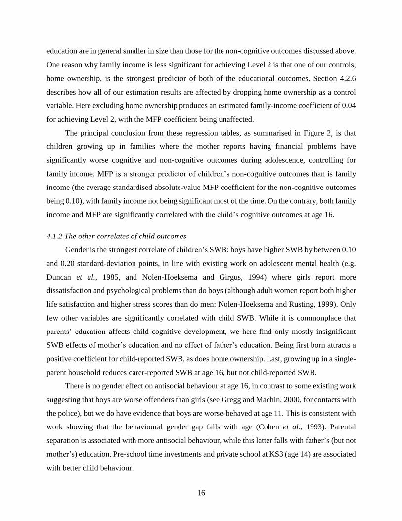
4.1.2 The other correlates of child outcomes

Gender is the strongest correlate of children’s SWB: boys have higher SWB by between 0.10

and 0.20 standard-deviation points, in line with existing work on adolescent mental health (e.g.

Duncan et al., 1985, and Nolen-Hoeksema and Girgus, 1994) where girls report more

dissatisfaction and psychological problems than do boys (although adult women report both higher

life satisfaction and higher stress scores than do men: Nolen-Hoeksema and Rusting, 1999). Only

few other variables are significantly correlated with child SWB. While it is commonplace that

parents’ education affects child cognitive development, we here find only mostly insignificant

SWB effects of mother’s education and no effect of father’s education. Being first born attracts a

positive coefficient for child-reported SWB, as does home ownership. Last, growing up in a single-

parent household reduces carer-reported SWB at age 16, but not child-reported SWB.

There is no gender effect on antisocial behaviour at age 16, in contrast to some existing work

suggesting that boys are worse offenders than girls (see Gregg and Machin, 2000, for contacts with

the police), but we do have evidence that boys are worse-behaved at age 11. This is consistent with

work showing that the behavioural gender gap falls with age (Cohen et al., 1993). Parental

separation is associated with more antisocial behaviour, while this latter falls with father’s (but not

mother’s) education. Pre-school time investments and private school at KS3 (age 14) are associated

with better child behaviour.

17

We find no gender effect on emotional health at age 11. Mother’s education has a positive

effect on child emotional health at age 11. The presence of other children in the household improves

both emotional health and behaviour, as do time investments and mother’s years of work.

More variables are significant in the teacher-reported version of the behaviour and emotional-

health table (Table A5.2). Boys again behave worse and (to a lesser extent) have worse emotional

health. White children also have lower emotional health. The first-born have better behaviour but

worse emotional health. Home ownership and parental education are associated with better teacher-

reported outcomes for almost all measures, while parental separation produces worse outcomes.

As for the carer-reported outcomes, mother’s employment is positively related to child emotional

health but not behaviour.

Apart from MFP, only few variables are correlated with BMI and we in particular find no

gender effect. We will consider some alternative physical health measures in Section 4.2.5 below.

Home ownership is amongst the strongest predictors of cognitive outcomes, with an effect

size of about 0.12 standard deviations. Girls, the first-born, and those with older mothers and better-

educated parents record better educational performance; the number of siblings and parental

separation are associated with lower test scores.

4.2 Extensions to the Baseline Results

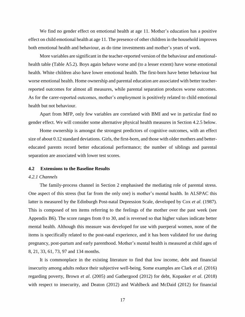
4.2.1 Channels

The family-process channel in Section 2 emphasised the mediating role of parental stress.

One aspect of this stress (but far from the only one) is mother’s mental health. In ALSPAC this

latter is measured by the Edinburgh Post-natal Depression Scale, developed by Cox et al. (1987).

This is composed of ten items referring to the feelings of the mother over the past week (see

Appendix B6). The score ranges from 0 to 30, and is reversed so that higher values indicate better

mental health. Although this measure was developed for use with puerperal women, none of the

items is specifically related to the post-natal experience, and it has been validated for use during

pregnancy, post-partum and early parenthood. Mother’s mental health is measured at child ages of

8, 21, 33, 61, 73, 97 and 134 months.

It is commonplace in the existing literature to find that low income, debt and financial

insecurity among adults reduce their subjective well-being. Some examples are Clark et al. (2016)

regarding poverty, Brown et al. (2005) and Gathergood (2012) for debt, Kopasker et al. (2018)

with respect to insecurity, and Deaton (2012) and Wahlbeck and McDaid (2012) for financial

18

crises. We do indeed find a correlation in ALSPAC data between mother’s mental health and both

MFP and income.

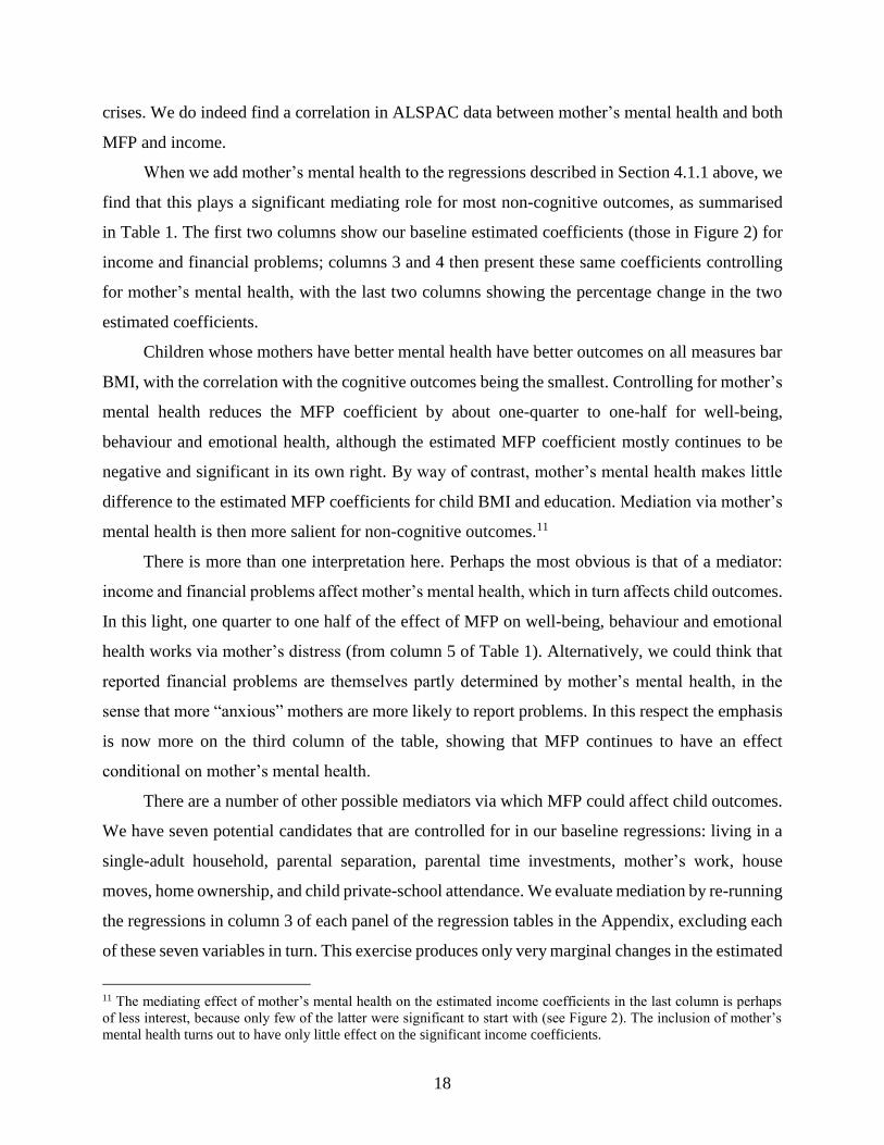
When we add mother’s mental health to the regressions described in Section 4.1.1 above, we

find that this plays a significant mediating role for most non-cognitive outcomes, as summarised

in Table 1. The first two columns show our baseline estimated coefficients (those in Figure 2) for

income and financial problems; columns 3 and 4 then present these same coefficients controlling

for mother’s mental health, with the last two columns showing the percentage change in the two

estimated coefficients.

Children whose mothers have better mental health have better outcomes on all measures bar

BMI, with the correlation with the cognitive outcomes being the smallest. Controlling for mother’s

mental health reduces the MFP coefficient by about one-quarter to one-half for well-being,

behaviour and emotional health, although the estimated MFP coefficient mostly continues to be

negative and significant in its own right. By way of contrast, mother’s mental health makes little

difference to the estimated MFP coefficients for child BMI and education. Mediation via mother’s

mental health is then more salient for non-cognitive outcomes.11

There is more than one interpretation here. Perhaps the most obvious is that of a mediator:

income and financial problems affect mother’s mental health, which in turn affects child outcomes.

In this light, one quarter to one half of the effect of MFP on well-being, behaviour and emotional

health works via mother’s distress (from column 5 of Table 1). Alternatively, we could think that

reported financial problems are themselves partly determined by mother’s mental health, in the

sense that more “anxious” mothers are more likely to report problems. In this respect the emphasis

is now more on the third column of the table, showing that MFP continues to have an effect

conditional on mother’s mental health.

There are a number of other possible mediators via which MFP could affect child outcomes.

We have seven potential candidates that are controlled for in our baseline regressions: living in a

single-adult household, parental separation, parental time investments, mother’s work, house

moves, home ownership, and child private-school attendance. We evaluate mediation by re-running

the regressions in column 3 of each panel of the regression tables in the Appendix, excluding each

of these seven variables in turn. This exercise produces only very marginal changes in the estimated

11 The mediating effect of mother’s mental health on the estimated income coefficients in the last column is perhaps

of less interest, because only few of the latter were significant to start with (see Figure 2). The inclusion of mother’s

mental health turns out to have only little effect on the significant income coefficients.

19

MFP coefficients: these variables are not behind the effect of MFP on child and adolescent

outcomes.

Last, we can tackle this issue in the opposite direction, and add more control variables that

may be behind MFP to the baseline regression. Following the significant bivariate correlations in

Appendix C, we thus add controls for the experience of mother’s illness, mother’s job loss and

partner’s job loss over the child’s first eleven years (calculated in the same way as our variable of

experience of MFP). The addition of these three new variables reduced the coefficient on MFP as

expected, but only by around 10% for most non-cognitive outcomes. The reduction in the estimated

MFP coefficient for cognitive outcomes was somewhat larger: parental job loss and illness may

play a more important role for adolescent exam results than they do for non-cognitive outcomes.

In general, there is much more behind MFP (in terms of its consequences on adolescent outcomes)

than is picked up by this array of early-life events.

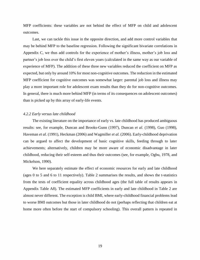
4.2.2 Early versus late childhood

The existing literature on the importance of early vs. late childhood has produced ambiguous

results: see, for example, Duncan and Brooks-Gunn (1997), Duncan et al. (1998), Guo (1998),

Haveman et al. (1991), Heckman (2006) and Wagmiller et al. (2006). Early-childhood deprivation

can be argued to affect the development of basic cognitive skills, feeding through to later

achievements; alternatively, children may be more aware of economic disadvantage in later

childhood, reducing their self-esteem and thus their outcomes (see, for example, Ogbu, 1978, and

Mickelson, 1990).

We here separately estimate the effect of economic resources for early and late childhood

(ages 0 to 5 and 6 to 11 respectively). Table 2 summarises the results, and shows the t-statistics

from the tests of coefficient equality across childhood ages (the full table of results appears in

Appendix Table A8). The estimated MFP coefficients in early and late childhood in Table 2 are

almost never different. The exception is child BMI, where early-childhood financial problems lead

to worse BMI outcomes but those in later childhood do not (perhaps reflecting that children eat at

home more often before the start of compulsory schooling). This overall pattern is repeated in

20

regressions that condition on mother’s mental health (results available on request). The effect of

income in the two childhood periods does not differ statistically for any outcome.12

4.2.3 Sub-group analyses

The pattern of our results is remarkably similar when we estimate boys’ and girls’ outcomes

separately: the differences refer to income and cognitive outcomes, and MFPs and teacher-reported

behaviour at age 11, both of which are only correlated for boys. This pattern of results chimes with

the gender difference in cognitive outcomes and behaviour following family disadvantage in Autor

et al. (2019) and the finding of no sex differences in the way in which negative cognitive style,

depression and rumination are correlated with an index of negative or stressful life events that

typically occur during adolescence in Hamilton et al. (2015). There are also no striking differences

for children in above- and below-median income households (where income refers to the average

household figure over the child’s first eleven years).13

4.2.4 Non-linearities

To see whether low values of MFP are unimportant, we cut the non-zero MFP distribution at

its median and created two dummy variables. From Figure 1, this median is at a value of around

1.7. We would in general expect the estimated coefficient for below-median MFPs to be smaller

than that on above-median MFPs. For a number of outcomes we find that the former is

insignificant. This is in particular the case for child-reported well-being, and both cognitive

outcomes. For these variables, a small number of MFPs does not matter: the overall negative MFP

coefficient listed in Table 1 rather comes from those children whose mothers experienced repeated

financial problems.

4.2.5 Alternative physical health measures

Physical health above was measured a dummy variable for child BMI being between the 5th

and 85th percentiles by age and sex. We also ran all of our analyses considering only the upper tail

12 We also experimented with decay functions, weighting MFPs at the different child ages by the ratio of child age at

MFP report to child age at outcome, which gives more weight to more recent MFPs, or by the complement of this

expression, giving more weight to earlier MFPs. The fit of the regressions (as measured by the R-squared) barely

changed. 13 Four out of 28 estimated MFP and income coefficients are significantly different between above- and below-median

households.

21

of the BMI distribution, i.e. a dummy for being above the 85th percentile of the specific gender-

age distribution. This made no difference to the results.

We also have information on a number of child physical health symptoms at age 11 (such as

stomach ache, arms/legs ache, cough at night, infection and asthma). We construct a dummy

variable for the total number of symptoms being in the top 40% of the distribution (as in Propper

et al., 2007) and also look at the total number of symptoms. Last, we have information on the

general health of the child as assessed by the mother, and create a dummy for the child being

anything other than very healthy. The results for both of the symptoms variables mirror those for

BMI: the number of major financial problems attracts a positive estimated coefficient that is

significant at the one per cent level while that on income is insignificant.14 Regarding child overall

health at age 11, both MFP and income attract significant estimated coefficients of roughly equal

size.

4.2.6 Income and Wealth

All of our results above concerning income and MFP come from regressions which condition

on a range of control variables, including home ownership. This latter is often considered as a

measure of wealth. To check whether any correlation between wealth and income (or indeed

between wealth and MFP) is affecting our conclusions, we have re-run our regressions dropping

home ownership. This makes almost no difference to the estimated MFP coefficients that are

summarised in Table 1. It also does not affect our conclusions regarding the correlation between

income and child non-cognitive outcomes. Where it does make a difference is for income and

cognitive outcomes. Home ownership is one of the strongest predictors of both of our educational

outcomes (see Table 7A), and its exclusion from the child-education regressions leads to estimated

income coefficients that are almost double the size of those in Table 1.

4.2.7 Issues in Imputation

Both the income and financial-problems variables in the regressions contain some imputed

values. The distribution of financial problems including imputed values in Figure 1 shows a slight

uptick at the maximum value of 10. This almost never reflects a respondent reporting problems ten

14 Janssen and Sandner (2016) exploit information on a German welfare reform and also find no effect of household

income on young child health.

22

times, but rather someone who is interviewed four times (say), reports a financial problem each

time, and then has an imputed value of 10 (as 4 x 10/4). All of our results are robust to dropping

this maximum category in our adolescent-outcome regressions.

Along the same lines, it might be thought that imputing missing values produces an over-

estimation of the incidence of financial problems. As an experiment, we instead replace all missing

values by zero, including the financial-problems score of those who are missing at every wave with

respect to this variable: this undoubtedly produces an under-estimate of incidence. The “missing

as zero” estimation results reveal smaller estimated coefficients on financial problems, all of which

remain significant and mostly larger than those on income (which hardly change).

Our approach to missing income information was to calculate the average of the five reported

values over childhood. If fewer than five were reported, we took the average over the reported

figures only (which amounts to replacing the missing information by the individual-level mean). If

all five were missing, we replaced by the sample mean and created a missing income flag. Around

23% of observations were missing income at all waves. We first check that our results remain

unchanged when we simply drop this 23% group. This produces estimated coefficients on income

that are sometimes larger than those in our main results, but broadly does not change their pattern.

Notably the income coefficients for cognitive outcomes are now considerably larger than those on

financial problems (although all estimated coefficients remain significant at the five per cent level

or better).

We have also changed the imputation approach for all variables from missing indicator to

multiple imputation.15 The estimated results again remain similar (although, as above, the estimated

income coefficients in the cognitive-outcome regressions are notably larger).

4.2.8 Falls in income and major financial problems

Our main results refer to financial problems and the level of household income, and we in

general underline the importance of the former over the latter (at least for the non-cognitive

outcomes). Although the level of income and MFP are only correlated at 0.16, we might imagine

that falls in income are a key cause of MFP. Due to the banded (and infrequent) nature of the

15 Multiple imputation was performed using chained equations with ten imputations, assuming that missing

observations are missing at random (MAR) given the known characteristics of the individuals for which observations

are missing. Estimates from the ten imputed datasets are then combined using Rubin’s rule. This approach has already

been used in other papers based on ALSPAC (see e.g. Washbroook et al., 2014).

23

ALSPAC income variable, we cannot observe these income drops directly. However, we do have

annual information on whether the mother reported a fall in income over the past year. We count

the number of years with an income drop. This count is correlated with the MFP variable at 0.5.

Regressions with income, MFP and income drops produce estimated coefficients on the first

two variables that are very similar to those summarised in Figure 2. For the non-cognitive

outcomes, income remains significant only for the two internalising SDQ variables at age 11, while

MFP remains significant for almost all non-cognitive outcomes with estimated coefficients that are

attenuated by only 10-20%. The results for the cognitive outcomes are not at all affected. The

income-drop variable itself is significantly correlated with all three well-being variables, the carer

and teacher-reported anti-social behaviour variables, and carer-reported child behaviour and

emotional health. The estimated coefficient on the (standardised) income-drop variable is always

smaller than that on standardised MFP.

4.3 Endogeneity Concerns

Our main results above related child outcomes at ages 16 or 18 to the financial problems

reported by their mothers between child ages 0 and 11. We here consider the evidence for this

relationship being causal. It will not be so if there is an omitted variable that predicts both MFP at

earlier ages and later child outcomes: this could perhaps be local socio-economic conditions or

parenting style.

A first point is that our regressions do control for a wide range of background characteristics.

In itself, this does not of course prove that there are no other omitted variables. Unfortunately, we

do not have any particularly good candidate variables with which to instrument MFP, especially as

we would need to do so over an eleven-year period. We cannot appeal to geographical variation as

the data come from relatively small area. Given the nature of the birth-cohort data we use here, we

also cannot sensibly use a family/sibling difference model, in which family fixed effects pick up

time-invariant family characteristics that are common to siblings (e.g. Ermisch et al., 2004;

Björklund and Sundström, 2006).16 We do have a few twins, but they are not helpful in this context

as they are of course exposed to the same MFP when growing up. There are in addition a very few

families with two births over the 18-month initial data-collection period, but not enough for any

16 The intuition here is that we can compare the test scores of siblings who experience different levels of MFP while

growing up.

24

sensible analysis (and these siblings, being born so close together, will have “almost” the same

MFP exposure over childhood).

We do however believe that we can make progress here by splitting childhood up into

separate time periods (0-5 years old and 5-11 years old), and estimating a value-added

specification. The worry is that all childhood outcomes are predicted by an unobserved variable,

Z, which is also correlated with MFP. In order to help turn this channel off, we will add earlier

child outcomes to our main estimation equation: we estimate child adolescent outcomes controlling

now for child outcomes at ages 4-5 and the MFPs that the child experienced between the ages of 6

and 11.

If there is an omitted variable of this kind, or if indeed there is reverse causality, whereby a

shock to earlier child outcomes (that are serially correlated over time) produces later major

financial problems, then we will be able to predict MFP between ages 6 and 11 from young child

outcomes.

The regression results show that both internalizing and externalizing SDQ at age 4 are

significant predictors of MFP between the ages of 6 and 11: worse scores in both dimensions are

associated with more MFP’s later in childhood. The same conclusion is found for the child’s Key

Stage One scores (at age 6), but neither for their poor health at age 5 (carer-reported) nor for the

number of health symptoms at the same age.

To evaluate whether our correlations in Figure 2 entirely reflect reverse causality or an

omitted variable, we re-estimate our child outcomes (that are mostly at age 16/18), as a function of

MFPs aged 6-11 and Child outcomes at ages 4 or 5 in a value-added model. The intuitive argument

is that any omitted variables, Z, that predict both child outcomes and parental MFP will be picked

up by the earlier child outcomes. The equation we estimate here is as follows:

𝐶𝑂𝑖 = 𝛼 + 𝛽𝑀𝐹𝑃𝑖6−11 + 𝛾𝑙𝑛𝑌𝑖

6−11 + 𝜃𝐶𝑂𝑖4−5 + 𝛿𝑋𝑖 + 휀𝑖 (2)

The results appear in Table 3. There were 14 original estimated MFP coefficients, as

summarised in Figure 2 (and which re-appear in column 1 of Table 3). Of these, 13 were significant

and of the “correct” sign. Column 3 of Table 3 shows the analogous estimates from the estimation

of equation (2) above. Of these 14 new estimated coefficients, 10 are of the correct sign and

significant (even though we lose statistical power, as there is less variation in MFP between ages

25

6-11 than in MFP ages 0-11). In particular, the results for the three well-being variables and carer-

reported behaviour and emotional health all continue to hold. The results for the two teacher-

reported behaviours are even a little stronger in this new specification. We lose significance for

teacher-reported emotional health at age 11 and one of the two education outcomes (that which

was the least significant in Figure 2). In addition, only one of the three BMI outcomes remains

significant.

As in Section 4.2.5 above, we can replace BMI as a health outcome by either carer-reported

poor child health at ages 11 and 13, or the number of physical health symptoms at age 11. For the

first two of these, the child-outcome regression controls for poor child health at age 5, while for

the latter it is the number of health problems at age 5. The results at the bottom of the non-cognitive

panel of Table 3 show that MFP between 6 and 11 continue to predict later child health outcomes

even controlling for child health at age 5.

In the estimation of equation (2) we treat income analogously to MFP, and replace its value

over the whole of childhood with its value from ages 6 through 11 only. The estimated coefficients

on income in later childhood appear in column 4 of Table 3: these are to be compared to those in

the initial analysis in column 2 of Table 1. There is no effect on the significance of the first six

outcome variables (for which only one estimated coefficient is significant). For the teacher-

reported behavioural and emotional outcomes, again only one of the three estimated coefficients is

significant (although not the same one), while for BMI none of the three income coefficients is

significant.

The biggest change relative to Table 1 regards the correlation between childhood income and

adolescent cognitive outcomes. The correlations in Table 1 were both positive and significant, and

especially so for average GCSE points. Once we control for Key Stage 1 outcomes at age 6, there

is no additional effect of income between ages 6 and 11 on the child’s age-16 exam outcomes.

The finding that income plays little role in the determination of cognitive outcomes is worthy

of comment. One interpretation is that income (as opposed to MFP) only matters in early childhood,

although this was not evident at the bottom of Table 2. Another is that income does continue to

affect child cognitive outcomes, but only for certain groups. To investigate, we interacted income

between child ages 6 and 11 with a dummy variable for having below median income at ages 0-5.

There is almost no evidence of a moderated effect of income at ages 6-11 on any of the non-

cognitive outcomes. The results for the two cognitive outcomes at age 16 however reveal a

26

significant effect for income at ages 6-11 on the cognitive outcomes of children whose household

income at ages 0-5 was below the median. As in Akee et al. (2018), the effect of income on child

outcomes may be much more striking in relatively-deprived households.

The overall picture here then is similar to that from our initial analysis: controlling for

income, childhood financial problems are significantly correlated with adolescent outcomes (and

these adolescent outcomes are major predictors of well-being throughout the life course: see Clark

et al., 2018).

5. Conclusion

Financial insecurity and stress are central determinants of well-being. We here use large-scale long-

run birth-cohort data to make two central contributions in this context. We first extend the typical

contemporaneous analysis by relating parental financial insecurity experienced during childhood

to a range of cognitive and non-cognitive outcomes experienced by the children during the

intermediate period of adolescence. Second, we do not limit ourselves to income as the sole

measure of financial stress, but also consider the incidence of financial problems as reported by the

mother. Our broad premise is that income alone may be an insufficient indicator of the sufficiency

of economic resources.

This premise is borne out in the empirical results. All of our adolescent non-cognitive

outcomes are significantly correlated with childhood financial problems, but few are correlated

with childhood income. On the contrary, adolescent cognitive outcomes are correlated with both

financial problems and income. While we then agree with Duncan and Brooks-Gunn (1997) that

non-cognitive outcomes are less sensitive to family income than are cognitive outcomes, we

notably find exactly the opposite ordering with respect to family financial problems.

Our results underline that childhood financial problems are significantly correlated with most

adolescent outcomes, even after controlling for family income. This correlation does not seem to

be subject to contamination by mood, as the reports of financial problems and child outcomes are

separated by a period of up to 17 years. In addition, we find correlations not only with mother’s

reports of adolescent outcomes but also with those reported by the adolescent him/herself and by

teachers. Last, our results continue to hold in value-added regressions controlling for children’s

initial outcomes at around age 5.

27

In the recent Great Recession, the types of financial problems that we analyse here have

arguably become more widespread than low income, and have spilled over to the middle-class as

well (as highlighted, for example, by Gauthier and Furstenberg, 2010, in relation to families with

children). The Federal Reserve’s Report on the Economic Well-Being of U.S. Households in 2014

highlighted that 24% of individuals had experienced some form of financial hardship over the past

year, and 47% could not cover an unexpected expense of $400. A December 2015 survey by

Bankrate17 found that 63% of Americans have no emergency savings for a $1000 emergency-room

visit or a $500 car repair, and a July 2016 UK survey by the housing charity Shelter18 that 37% of

working families would be unable to cover their housing expenses were one of the partners to lose

their jobs. This widespread financial insecurity undoubtedly has sharp effects on the well-being of

the individuals concerned; our work here also suggests that it may cast a long shadow over the

outcomes of their children many years in the future.

17 Bankrate: http://www.bankrate.com/finance/consumer-index/money-pulse-1215.aspx. 18 Shelter: http://www.bbc.com/news/uk-england-37017254.

28

References

Acemoglu, D., Pischke, J.-S., 2001. Changes in the wage structure, family income, and children's

education. European Economic Review 45, 890-904.

Akee, R., Copeland, W., Costello, E., Simeonova, E., 2018. How Does Household Income Affect

Child Personality Traits and Behaviors? American Economic Review 108, 775–827.

Akee, R., Copeland, W., Keeler, G., Angold, A., Costello, E., 2010. Parents' Incomes and

Children's Outcomes: A Quasi-experiment Using Transfer Payments from Casino Profits.

American Economic Journal: Applied Economics 2, 86-115.

Autor, D., Figlio, D., Karbownik, K., Roth, J., Wasserman, M., 2019. Family Disadvantage and

the Gender Gap in Behavioral and Educational Outcome. American Economic Journal:

Applied Economics, forthcoming.

Axinn, W., Duncan, G.J., Thornton, A., 1997. The effects of parents’ income, wealth, and attitudes

on children’s completed schooling and self-esteem.In G.J.Duncan, J.Brooks-Gunn (Eds.),

Consequences of growing up poor. New York: Russell Sage Foundation.

Bastian, J., Michelmore, K., 2018. The long-term impact of the earned income tax credit on

children’s education and employment outcomes. Journal of Labor Economics 36, 1127-

1163.

Becker, G.S., 1981. A Treatise on the Family. Cambridge MA: Harvard University Press.

Becker, G.S., Tomes, N., 1986. Human capital and the rise and fall of families. Journal of Labor

Economics 4, S1-S39.

Becker, G.S., Tomes, N., 1994. Human Capital: A Theoretical and Empirical Analysis with Special

Reference to Education (3rd Edition). Chicago: University of Chicago Press, 257-298.

Black, S.E., Devereux, P.J., Salvanes, K.G., 2005. The more the merrier? The effect of family size

and birth order on children's education. Quarterly Journal of Economics 120, 669-700.

Blanden, J., Gregg, P., 2004. Family income and educational attainment: a review of approaches

and evidence for Britain. Oxford Review of Economic Policy 20, 245-263.

Blau, D.M., 1999. The effect of income on child development. Review of Economics and Statistics

81, 261-276.

Bolger, K.E., Patterson, C.J., Thompson, W.W., Kupersmidt, J.B., 1995. Psychosocial adjustment

among children experiencing persistent and intermittent family economic hardship. Child

Development 66, 1107-1129.

Bossert, W., D'Ambrosio, C., 2013. Measuring Economic Insecurity. International Economic

Review 54, 1017-1030.

Brown, S., Taylor, K., Wheatley-Price, S., 2005. Debt and distress: Evaluating the psychological

cost of credit. Journal of Economic Psychology 26, 642-663.

Case, A., Paxson, C., 2002. Parental behavior and child health. Health Affairs 21, 164-178.

Clark, A.E., D'Ambrosio, C., Ghislandi, S., 2016. Adaptation to Poverty in Long-Run Panel Data.

Review of Economics and Statistics 98, 591-600.

29

Clark, A.E., Flèche, S., Layard, R., Powdthavee, N., Ward, G., 2018. The Origins of Happiness:

The Science of Well-Being over the Life-Course. Princeton NJ: Princeton University Press.

Conger, R.D., Conger, K.J., Martin, M.J., 2010. Socioeconomic Status, Family Processes,and

Individual Development. Journal of Marriage and the Family 72, 685-704.

Cohen, P., Cohen, J., Kasen, S., Velez, C.N., Hartmark, C., Johnson, J., Rojas, M., Brook, J.,

Streuning, E., 1993. An Epidemiological Study of Disorders in Late Childhood and

Adolescence I. Age- and Gender- Specific Prevalence. Journal of Child Psychology and

Psychiatry 34, 851-867.

Cox, J.L., Holden, J.M., Sagovsky, R., 1987. Detection of postnatal depression. Development of

the 10-item Edinburgh Postnatal Depression Scale. British Journal of Psychiatry 150, 782-

786.

Currie, J., Stabile, M., 2003. Socioeconomic status and health: why is the relationship stronger for

older children?. American Economic Review, 93, 1813-1823.

Dahl, G., Lochner, L., 2012. The impact of family income on child achievement: evidence from

the earned income tax credit. American Economic Review 102, 1972-56.

Deaton, A., 2012. The financial crisis and the well-being of Americans. Oxford Economic Papers

64, 1-26.

Duncan, G.J., Brooks-Gunn, J., 1997. Consequences of growing up poor. New York: Russell Sage

Foundation.

Duncan, G., Magnuson, K., Votruba-Drzal, E., 2017. Moving Beyond Correlations in Assessing

the Consequences of Poverty. Annual Review of Psychology 68, 413-434.

Duncan, P.D., Ritter, P.L., Dornbusch, S.M., Gross, R.T., Carlsmith, J.M., 1985. The effects of

pubertal timing on body image, school behavior, and deviance. Journal of Youth and

Adolescence 14, 227-235.

Duncan, G.J., Yeung, W.J., Brooks-Gunn, J., Smith, J.R., 1998. How much does childhood poverty

affect the life chances of children? American Sociological Review 63, 406-423.

Elder, J., 1997. Children of the Great Depression. 25th Anniversary Edition. Boulder, CO:

Westview Press.

Ermisch, J., Francesconi, M., 2001. Family matters: Impacts of family background on educational

attainments. Economica 68, 137-156.

Evans, G., Cassells, R., 2014. Childhood Poverty, Cumulative Risk Exposure, and Mental Health

in Emerging Adults. Clinical Psychological Science, 2, 287-296.

Feinstein, L., 2000. The relative economic importance of academic, psychological and behavioural

attributes developed on childhood. Centre for Economic Performance, London School of

Economics and Political Science.

Flèche, S., Lekfuangfu, W., Clark, A.E., 2019. The long-lasting effects of childhood on adult

wellbeing: Evidence from British cohort data. Journal of Economic Behavior and

Organization, forthcoming.

30

Ford, T., Goodman, R., Meltzer, H., 2004. The relative importance of child, family, school and

neighbourhood correlates of childhood psychiatric disorder. Social Psychiatry and Psychiatric

Epidemiology, 39, 487-496.

Gathergood, J., 2012. Debt and Depression: Causal Links and Social Norm Effects. Economic

Journal 122, 1094-1114.

Gauthier, A.H., Furstenberg, F.F., 2010. The experience of financial strain among families with

children in the United States. National Center for Family & Marriage Research, Working Paper

WP-10-17.

Goodman, R., Lamping, D. L., Ploubidis, G. B., 2010. When to use broader internalising and

externalising subscales instead of the hypothesised five subscales on the Strengths and

Difficulties Questionnaire (SDQ): data from British parents, teachers and children. Journal of

Abnormal Child Psychology 38, 1179-1191.

Gregg, P., Machin, S., 2000. Child development and success or failure in the youth labor market.

NBER Comparative Labour Market Series. Chicago: University of Chicago Press, 247-288.

Guo, G., 1998. The timing of the influences of cumulative poverty on children's cognitive ability

and achievement. Social Forces 77, 257-287.

Guo, G., Harris, K.M., 2000. The mechanisms mediating the effects of poverty on children’s

intellectual development. Demography 37, 431-447.

Hamilton, J., Stange, J., Abramson, L., Alloy, L., 2015. Stress and the Development of Cognitive

Vulnerabilities to Depression Explain Sex Differences in Depressive Symptoms During

Adolescence. Clinical Psychological Science 3, 702-714.

Hardy, B.L., 2014. Childhood income volatility and adult outcomes. Demography 51, 1641-1665.

Haveman, R., Wolfe, B., 1995. The determinants of children's attainments: A review of methods

and findings. Journal of Economic Literature 33, 1829-1878.

Haveman, R., Wolfe, B., Spaulding, J., 1991. Childhood events and circumstances influencing high

school completion. Demography 28, 133-157.

Heckman, J.J., 2006. Skill formation and the economics of investing in disadvantaged children.

Science 312, 1900-1902.

Heckman, J.J., Stixrud, J., Urzua, S., 2006. The effects of cognitive and noncognitive abilities on

labor market outcomes and social behavior. Journal of Labor Economics 24, 411-82.

Hilger, N., 2016. Parental job loss and children’s long-term outcomes: evidence from 7 million

fathers’ layoffs. American Economic Journal: Applied Economics 8, 247-283.

Hoynes, H., Whitmore Schanzenbach, D., Almond, D., 2016. Long-run impacts of childhood

access to the safety net. American Economic Review 106, 903-34.

Janssen, S., Sandner, M., 2016. Household Income and Infant Health. Evidence from a Welfare

Benefits Reform. IAB Nuremberg, mimeo.

Kalil, A., 2013. Effects of the Great Recession on Child Development. Annals AAPSS 650, 232-

249.

31

Kim, Y., Sherraden, M., 2011. Do parental assets matter for children's educational attainment?:

Evidence from mediation tests. Children and Youth Services Review 33, 969-979.

Kopasker, D., Montagna, C., Bender, K., 2018. Economic Insecurity as a Socioeconomic

Determinant of Mental Health. SSM - Population Health 6, 184-194.

Layard, R., Clark, A.E., Cornaglia, F., Powdthavee, N., Vernoit, J., 2014. What Predicts a

Successful Life? A Life-Course Model of Wellbeing. Economic Journal 124, F720- F738.

Matsumoto, B., 2018. Family Ruptures, Stress, and the Mental Health of the Next Generation:

Comment. American Economic Review 108, 1253-55.

Maurin, E., 2002. The impact of parental income on early schooling transitions: A re-examination

using data over three generations. Journal of Public Economics 85, 301-332.

Mayer, S.E., 1997. What money can't buy: Family income and children's life chances. Cambridge,

MA: Harvard University Press.

McLeod, J.D., Shanahan, M.J., 1993. Poverty, parenting, and children's mental health. American

Sociological Review 58, 351-366.

McLoyd, V.C., 1990. The impact of economic hardship on black families and children:

Psychological distress, parenting, and socioemotional development. Child Development 61,

311-346.

McLoyd, V.C., 1998. Socioeconomic disadvantage and child development. American Psychologist

53, 185-204.

Mickelson, R.A., 1990. The attitude-achievement paradox among Black adolescents. Sociology of

Education 63, 44-61.

Mistry, R.S., Vandewater, E.A., Huston, A.C., McLoyd, V.C., 2002. Economic Well-Being and

Children's Social Adjustment: The Role of Family Process in an Ethnically Diverse Low-

Income Sample. Child Development 73, 935-951.

Nolen-Hoeksema, S., Girgus, J.S., 1994. The emergence of gender differences in depression during

adolescence. Psychological Bulletin 115, 424-443.

Nolen-Hoeksema, S., Rusting, C.L., 1999. Gender differences in well-being. In D. Kahneman, E.

Diener, and N. Schwartz (Eds.), Well-being: The foundations of hedonic psychology. New

York: Russell Sage Foundation.

Ogbu, J.U., 1978. Minority education and caste: The American system in cross-cultural

perspective. New York: Academic Press.

Oreopoulos, P., Page, M., Stevens, A., 2008. The Intergenerational Effects of Worker

Displacement. Journal of Labor Economics 26, 455-483.

Persson, P., Rossin-Slater, M., 2018. Family Ruptures, Stress, and the Mental Health of the Next

Generation. American Economic Review 108, 1214-52.

Propper, C., Rigg, J., Burgess, S., 2007. Child health: evidence on the roles of family income and

maternal mental health from a UK birth cohort. Health Economics, 16, 1245-1269.

Rege, M., Telle, K., Votruba, M., 2011. Parental job loss and children’s school performance.

Review of Economic Studies 78, 1462-89.

32

Shriver, M., 2014. The Shriver Report: A Woman's Nation Pushes Back from the Brink. Free Press.

Available at http://shriverreport.org/a-womans-nation-pushes-back-from-the-brink-executive-

summary-maria-shriver/.

Shea, J., 2000. Does parents’ money matter? Journal of Public Economics 77, 155-184.

Sobolewski, J.M., Amato, P.R., 2005. Economic Hardship in the Family of Origin and Children’s

Psychological Well-Being in Adulthood. Journal of Marriage and Family 67, 141-156.

Stevens, A., Schaller, J., 2011. Short-run effects of parental job loss on children's academic

achievement. Economics of Education Review 30, 289-299.

Stiglitz, J. E., Sen, A., Fitoussi, J.-P. (2009). Report by the Commission on the Measurement of

Economic Performance and Social Progress. Available at: http://www.stiglitz-sen-

fitoussi.fr/documents/rapport_anglais.pdf

Voydanoff, P., 1990. Economic Distress and Family Relations: A Review of the Eighties. Journal

of Marriage and Family 52, 1099-1115.

Wagmiller, R.L., Lennon, M.C., Kuang, L., Alberti, P.M., Aber, J.L., 2006. The dynamics of

economic disadvantage and children's life chances. American Sociological Review 71, 847-

866.

Wahlbeck, K., McDaid, D., 2012. Actions to alleviate the mental health impact of the economic

crisis. World Psychiatry, 11, 139-145.

Washbrook, E., Gregg, P., Propper, C., 2014. A decomposition analysis of the relationship between

parental income and multiple child outcomes. Journal of the Royal Statistical Society: Series

A (Statistics in Society) 177, 757-782.

Wickrama, K.A.S., Conger, R.D., Abraham, W.T., 2005. Early Adversity and Later Health: The

Intergenerational Transmission of Adversity Through Mental Disorder and Physical Illness.

Journals of Gerontology: Series B 60B, 125-129.

Yeung, W.J., Conley, D., 2008. Black–white achievement gap and family wealth. Child

Development 79, 303-324.

Yeung, W.J., Linver, M.R., Brooks-Gunn, J., 2002. How money matters for young children's

development: Parental investment and family processes. Child Development 73, 1861-1879.

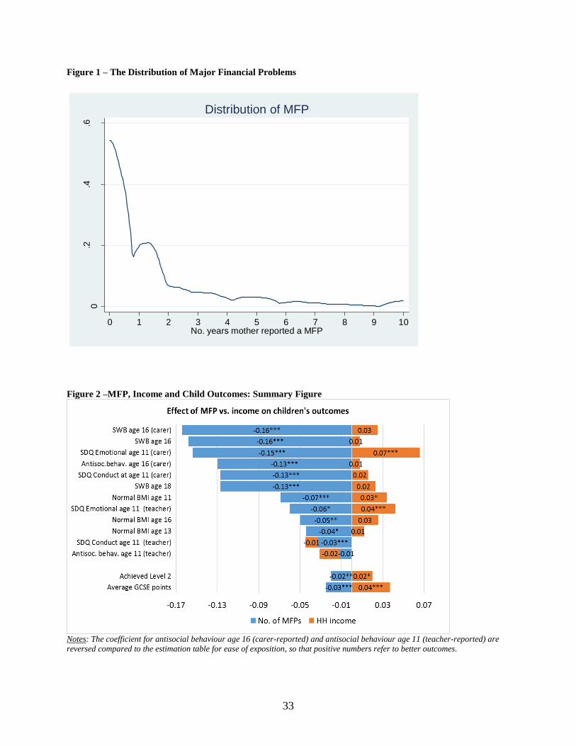
33

Figure 1 – The Distribution of Major Financial Problems

Figure 2 –MFP, Income and Child Outcomes: Summary Figure

Notes: The coefficient for antisocial behaviour age 16 (carer-reported) and antisocial behaviour age 11 (teacher-reported) are

reversed compared to the estimation table for ease of exposition, so that positive numbers refer to better outcomes.

0.2

.4.6

De

nsity

0 1 2 3 4 5 6 7 8 9 10No. years mother reported a MFP

Distribution of MFP

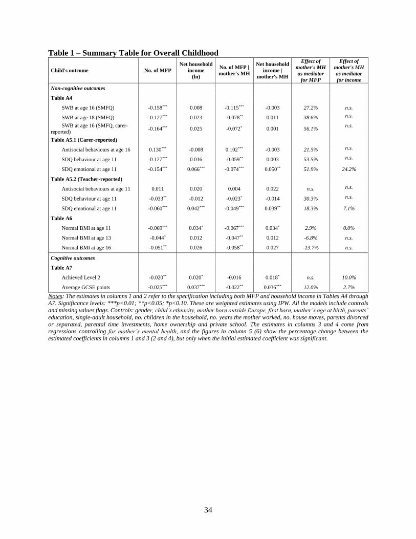
34

Table 1 – Summary Table for Overall Childhood

Child's outcome No. of MFP

Net household

income

(ln)

No. of MFP |

mother's MH

Net household

income |

mother's MH

Effect of

mother's MH

as mediator

for MFP

Effect of

mother's MH

as mediator

for income

Non-cognitive outcomes

Table A4

SWB at age 16 (SMFQ) -0.158*** 0.008 -0.115*** -0.003 27.2% n.s.

SWB at age 18 (SMFQ) -0.127*** 0.023 -0.078** 0.011 38.6% n.s.

SWB at age 16 (SMFQ, carer-

reported) -0.164*** 0.025 -0.072* 0.001 56.1%

n.s.

Table A5.1 (Carer-reported)

Antisocial behaviours at age 16 0.130*** -0.008 0.102*** -0.003 21.5% n.s.

SDQ behaviour at age 11 -0.127*** 0.016 -0.059** 0.003 53.5% n.s.

SDQ emotional at age 11 -0.154*** 0.066*** -0.074*** 0.050** 51.9% 24.2%

Table A5.2 (Teacher-reported)

Antisocial behaviours at age 11 0.011 0.020 0.004 0.022 n.s. n.s.

SDQ behaviour at age 11 -0.033** -0.012 -0.023* -0.014 30.3% n.s.

SDQ emotional at age 11 -0.060*** 0.042*** -0.049*** 0.039** 18.3% 7.1%

Table A6

Normal BMI at age 11 -0.069*** 0.034* -0.067*** 0.034* 2.9% 0.0%

Normal BMI at age 13 -0.044* 0.012 -0.047** 0.012 -6.8% n.s.

Normal BMI at age 16 -0.051** 0.026 -0.058** 0.027 -13.7% n.s.

Cognitive outcomes

Table A7

Achieved Level 2 -0.020** 0.020* -0.016 0.018* n.s. 10.0%

Average GCSE points -0.025*** 0.037*** -0.022** 0.036*** 12.0% 2.7%

Notes: The estimates in columns 1 and 2 refer to the specification including both MFP and household income in Tables A4 through

A7. Significance levels: ***p<0.01; **p<0.05; *p<0.10. These are weighted estimates using IPW. All the models include controls

and missing values flags. Controls: gender, child’s ethnicity, mother born outside Europe, first born, mother’s age at birth, parents’

education, single-adult household, no. children in the household, no. years the mother worked, no. house moves, parents divorced

or separated, parental time investments, home ownership and private school. The estimates in columns 3 and 4 come from

regressions controlling for mother’s mental health, and the figures in column 5 (6) show the percentage change between the

estimated coefficients in columns 1 and 3 (2 and 4), but only when the initial estimated coefficient was significant.

35

Table 2 – Summary Table Distinguishing Between Early and Late Childhood

Child's outcome No. of MFP T-test

(p-value)

Net household income (ln) T-test

(p-value)

Age 0-5 Age 6-11 Age 0-5 Age 6-11

Non-cognitive outcomes

SWB at age 16 (SMFQ) -0.104*** -0.041 0.253 -0.024 0.032 0.323

SWB at age 18 (SMFQ) -0.088*** -0.029 0.228 0.045 -0.003 0.408

SWB at age 16 (SMFQ, carer) -0.053* -0.128*** 0.176 0.032 -0.004 0.507

Antisoc. behav. age 16 (Carer) 0.059*** 0.075** 0.686 -0.013 -0.005 0.833

SDQ behaviour age 11 (Carer) -0.078*** -0.044** 0.228 0.021 0.005 0.408

SDQ emotional age 11 (Carer) -0.082*** -0.062*** 0.575 0.038 0.003 0.821

Antisoc. behav. age 11 (Teacher) -0.003 0.036** 0.081 0.003 0.018 0.627

SDQ behaviour age 11 (Teacher) -0.018 -0.026** 0.675 0.003 -0.011 0.581

SDQ emotional age 11 (Teacher) -0.035** -0.023 0.600 0.040** 0.022 0.548

Normal BMI age 11 -0.038* -0.026 0.728 0.035 0.019 0.681

Normal BMI age 13 -0.038* 0.002 0.225 0.009 0.005 0.910

Normal BMI age 16 -0.062*** 0.021 0.009 0.043* -0.007 0.217

Cognitive outcomes

Achieved Level 2 -0.008 -0.024** 0.325 0.007 0.014 0.750

Average GCSE points -0.013 -0.006 0.643 0.041*** 0.035*** 0.736

Notes: The dependent variable appears in the first column. Significance levels: ***p<0.01; **p<0.05; *p<0.10. Weighted estimates

using IPW. All of the models include controls and missing values flag. Controls: gender, child’s ethnicity, mother born outside

Europe, first born, mother’s age at birth, parents’ education, single-adult household, no. children in the household, no. years the

mother worked, no. house moves, parents divorced or separated, parental time investments, private school, and home ownership.

In columns 3 and 6, significant differences at the ten per cent level are indicated in bold.

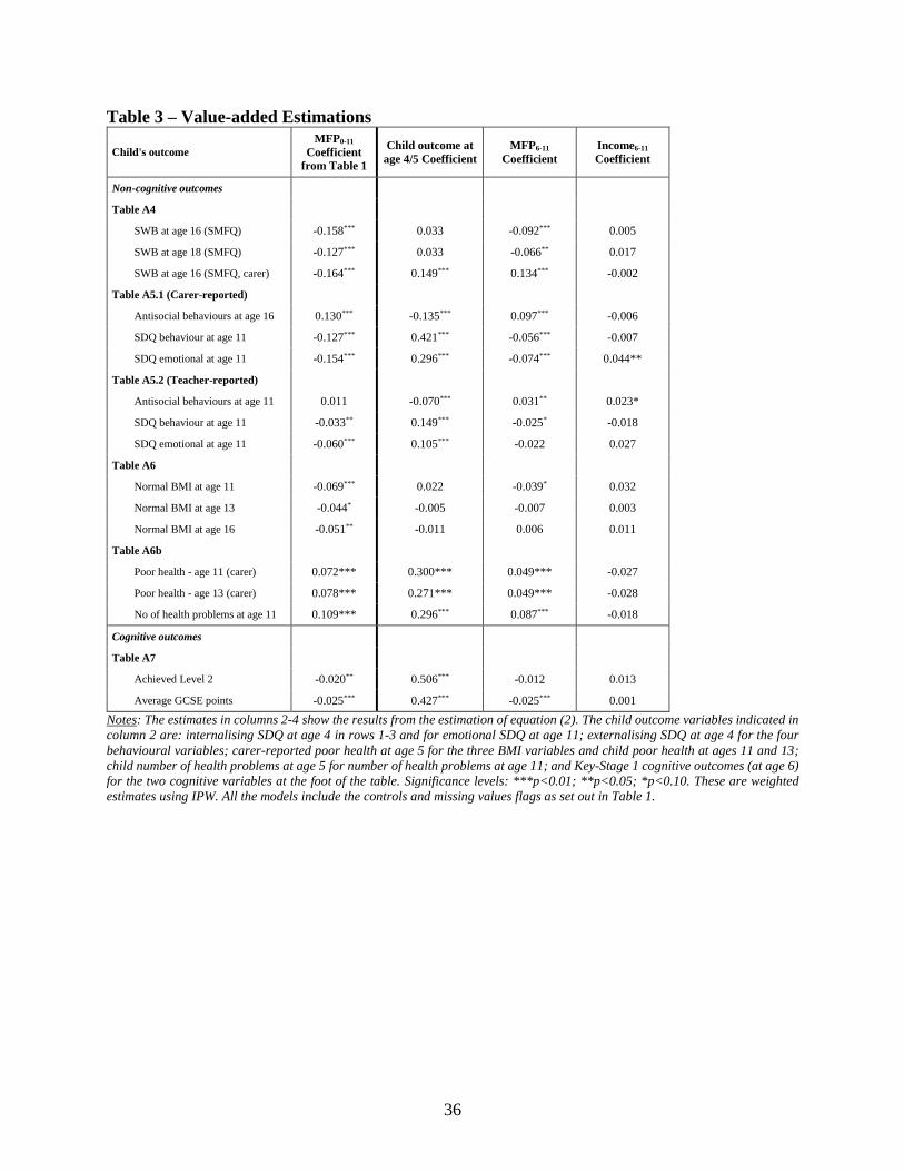
36

Table 3 – Value-added Estimations

Child's outcome

MFP0-11

Coefficient

from Table 1

Child outcome at

age 4/5 Coefficient

MFP6-11

Coefficient

Income6-11

Coefficient

Non-cognitive outcomes

Table A4

SWB at age 16 (SMFQ) -0.158*** 0.033 -0.092*** 0.005

SWB at age 18 (SMFQ) -0.127*** 0.033 -0.066** 0.017

SWB at age 16 (SMFQ, carer) -0.164*** 0.149*** 0.134*** -0.002

Table A5.1 (Carer-reported)

Antisocial behaviours at age 16 0.130*** -0.135*** 0.097*** -0.006

SDQ behaviour at age 11 -0.127*** 0.421*** -0.056*** -0.007

SDQ emotional at age 11 -0.154*** 0.296*** -0.074*** 0.044**

Table A5.2 (Teacher-reported)

Antisocial behaviours at age 11 0.011 -0.070*** 0.031** 0.023*

SDQ behaviour at age 11 -0.033** 0.149*** -0.025* -0.018

SDQ emotional at age 11 -0.060*** 0.105*** -0.022 0.027

Table A6

Normal BMI at age 11 -0.069*** 0.022 -0.039* 0.032

Normal BMI at age 13 -0.044* -0.005 -0.007 0.003

Normal BMI at age 16 -0.051** -0.011 0.006 0.011

Table A6b

Poor health - age 11 (carer) 0.072*** 0.300*** 0.049*** -0.027

Poor health - age 13 (carer) 0.078*** 0.271*** 0.049*** -0.028

No of health problems at age 11 0.109*** 0.296*** 0.087*** -0.018

Cognitive outcomes

Table A7

Achieved Level 2 -0.020** 0.506*** -0.012 0.013

Average GCSE points -0.025*** 0.427*** -0.025*** 0.001

Notes: The estimates in columns 2-4 show the results from the estimation of equation (2). The child outcome variables indicated in

column 2 are: internalising SDQ at age 4 in rows 1-3 and for emotional SDQ at age 11; externalising SDQ at age 4 for the four

behavioural variables; carer-reported poor health at age 5 for the three BMI variables and child poor health at ages 11 and 13;

child number of health problems at age 5 for number of health problems at age 11; and Key-Stage 1 cognitive outcomes (at age 6)

for the two cognitive variables at the foot of the table. Significance levels: ***p<0.01; **p<0.05; *p<0.10. These are weighted

estimates using IPW. All the models include the controls and missing values flags as set out in Table 1.

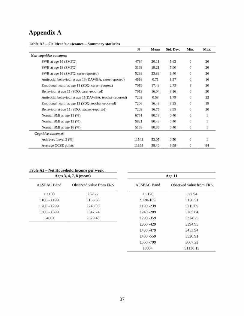
37

Appendix A Table A2 – Children’s outcomes – Summary statistics

N Mean Std. Dev. Min. Max.

Non-cognitive outcomes

SWB at age 16 (SMFQ) 4784 20.11 5.62 0 26

SWB at age 18 (SMFQ) 3193 19.21 5.90 0 26

SWB at age 16 (SMFQ, carer-reported) 5238 23.88 3.40 0 26

Antisocial behaviour at age 16 (DAWBA, carer-reported) 4516 0.71 1.57 0 16

Emotional health at age 11 (SDQ, carer-reported) 7019 17.43 2.73 3 20

Behaviour at age 11 (SDQ, carer-reported) 7013 16.04 3.16 0 20

Antisocial behaviour at age 11(DAWBA, teacher-reported) 7202 0.58 1.79 0 22

Emotional health at age 11 (SDQ, teacher-reported) 7206 16.43 3.25 0 19

Behaviour at age 11 (SDQ, teacher-reported) 7202 16.75 3.95 0 20

Normal BMI at age 11 (%) 6751 80.18 0.40 0 1

Normal BMI at age 13 (%) 5821 80.43 0.40 0 1

Normal BMI at age 16 (%) 5159 80.36 0.40 0 1

Cognitive outcomes

Achieved Level 2 (%) 11543 53.05 0.50 0 1

Average GCSE points 11393 38.40 9.98 0 64

Table A2 – Net Household Income per week

Ages 3, 4, 7, 8 (mean) Age 11

ALSPAC Band Observed value from FRS

ALSPAC Band Observed value from FRS

< £100 £62.77 < £120 £72.94

£100 - £199 £153.38 £120-189 £156.51

£200 - £299 £248.03 £190 -239 £215.69

£300 - £399 £347.74 £240 -289 £265.64

£400+ £679.48 £290 -359 £324.25

£360 -429 £394.95

£430 -479 £453.94

£480 -559 £520.91

£560 -799 £667.22

£800+ £1130.13

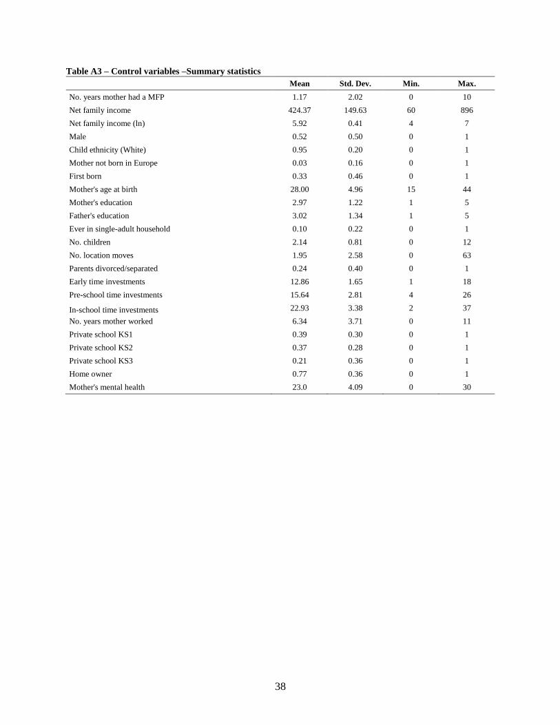
38

Table A3 – Control variables –Summary statistics

Mean Std. Dev. Min. Max.

No. years mother had a MFP 1.17 2.02 0 10

Net family income 424.37 149.63 60 896

Net family income (ln) 5.92 0.41 4 7

Male 0.52 0.50 0 1

Child ethnicity (White) 0.95 0.20 0 1

Mother not born in Europe 0.03 0.16 0 1

First born 0.33 0.46 0 1

Mother's age at birth 28.00 4.96 15 44

Mother's education 2.97 1.22 1 5

Father's education 3.02 1.34 1 5

Ever in single-adult household 0.10 0.22 0 1

No. children 2.14 0.81 0 12

No. location moves 1.95 2.58 0 63

Parents divorced/separated 0.24 0.40 0 1

Early time investments 12.86 1.65 1 18

Pre-school time investments 15.64 2.81 4 26

In-school time investments 22.93 3.38 2 37

No. years mother worked 6.34 3.71 0 11

Private school KS1 0.39 0.30 0 1

Private school KS2 0.37 0.28 0 1

Private school KS3 0.21 0.36 0 1

Home owner 0.77 0.36 0 1

Mother's mental health 23.0 4.09 0 30

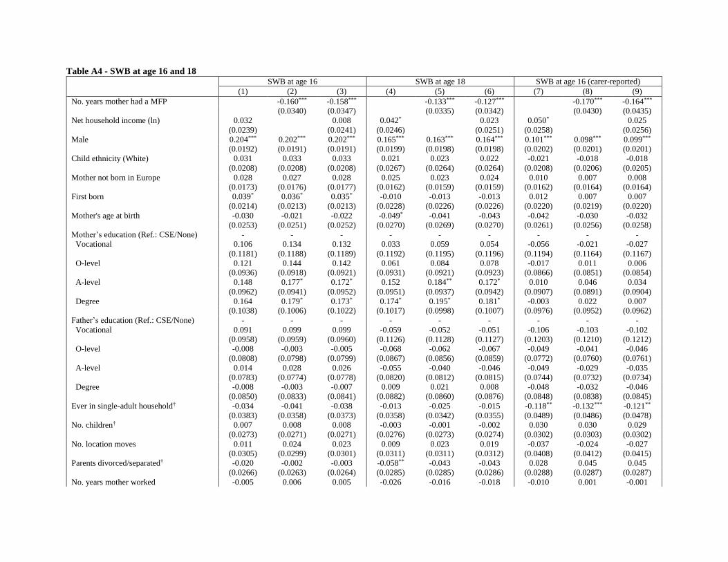
Table A4 - SWB at age 16 and 18 SWB at age 16 SWB at age 18 SWB at age 16 (carer-reported)

(1) (2) (3) (4) (5) (6) (7) (8) (9)

No. years mother had a MFP -0.160*** -0.158*** -0.133*** -0.127*** -0.170*** -0.164***

(0.0340) (0.0347) (0.0335) (0.0342) (0.0430) (0.0435)

Net household income (ln) 0.032 0.008 0.042* 0.023 0.050* 0.025

(0.0239) (0.0241) (0.0246) (0.0251) (0.0258) (0.0256)

Male 0.204*** 0.202*** 0.202*** 0.165*** 0.163*** 0.164*** 0.101*** 0.098*** 0.099***

(0.0192) (0.0191) (0.0191) (0.0199) (0.0198) (0.0198) (0.0202) (0.0201) (0.0201)

Child ethnicity (White) 0.031 0.033 0.033 0.021 0.023 0.022 -0.021 -0.018 -0.018

(0.0208) (0.0208) (0.0208) (0.0267) (0.0264) (0.0264) (0.0208) (0.0206) (0.0205)

Mother not born in Europe 0.028 0.027 0.028 0.025 0.023 0.024 0.010 0.007 0.008

(0.0173) (0.0176) (0.0177) (0.0162) (0.0159) (0.0159) (0.0162) (0.0164) (0.0164)

First born 0.039* 0.036* 0.035* -0.010 -0.013 -0.013 0.012 0.007 0.007

(0.0214) (0.0213) (0.0213) (0.0228) (0.0226) (0.0226) (0.0220) (0.0219) (0.0220)

Mother's age at birth -0.030 -0.021 -0.022 -0.049* -0.041 -0.043 -0.042 -0.030 -0.032

(0.0253) (0.0251) (0.0252) (0.0270) (0.0269) (0.0270) (0.0261) (0.0256) (0.0258)

Mother’s education (Ref.: CSE/None) - - - - - - - - -

Vocational 0.106 0.134 0.132 0.033 0.059 0.054 -0.056 -0.021 -0.027

(0.1181) (0.1188) (0.1189) (0.1192) (0.1195) (0.1196) (0.1194) (0.1164) (0.1167)

O-level 0.121 0.144 0.142 0.061 0.084 0.078 -0.017 0.011 0.006

(0.0936) (0.0918) (0.0921) (0.0931) (0.0921) (0.0923) (0.0866) (0.0851) (0.0854)

A-level 0.148 0.177* 0.172* 0.152 0.184** 0.172* 0.010 0.046 0.034

(0.0962) (0.0941) (0.0952) (0.0951) (0.0937) (0.0942) (0.0907) (0.0891) (0.0904)

Degree 0.164 0.179* 0.173* 0.174* 0.195* 0.181* -0.003 0.022 0.007

(0.1038) (0.1006) (0.1022) (0.1017) (0.0998) (0.1007) (0.0976) (0.0952) (0.0962)

Father’s education (Ref.: CSE/None) - - - - - - - - -

Vocational 0.091 0.099 0.099 -0.059 -0.052 -0.051 -0.106 -0.103 -0.102

(0.0958) (0.0959) (0.0960) (0.1126) (0.1128) (0.1127) (0.1203) (0.1210) (0.1212)

O-level -0.008 -0.003 -0.005 -0.068 -0.062 -0.067 -0.049 -0.041 -0.046

(0.0808) (0.0798) (0.0799) (0.0867) (0.0856) (0.0859) (0.0772) (0.0760) (0.0761)

A-level 0.014 0.028 0.026 -0.055 -0.040 -0.046 -0.049 -0.029 -0.035

(0.0783) (0.0774) (0.0778) (0.0820) (0.0812) (0.0815) (0.0744) (0.0732) (0.0734)

Degree -0.008 -0.003 -0.007 0.009 0.021 0.008 -0.048 -0.032 -0.046

(0.0850) (0.0833) (0.0841) (0.0882) (0.0860) (0.0876) (0.0848) (0.0838) (0.0845)

Ever in single-adult household† -0.034 -0.041 -0.038 -0.013 -0.025 -0.015 -0.118** -0.132*** -0.121**

(0.0383) (0.0358) (0.0373) (0.0358) (0.0342) (0.0355) (0.0489) (0.0486) (0.0478)

No. children† 0.007 0.008 0.008 -0.003 -0.001 -0.002 0.030 0.030 0.029

(0.0273) (0.0271) (0.0271) (0.0276) (0.0273) (0.0274) (0.0302) (0.0303) (0.0302)

No. location moves 0.011 0.024 0.023 0.009 0.023 0.019 -0.037 -0.024 -0.027

(0.0305) (0.0299) (0.0301) (0.0311) (0.0311) (0.0312) (0.0408) (0.0412) (0.0415)

Parents divorced/separated† -0.020 -0.002 -0.003 -0.058** -0.043 -0.043 0.028 0.045 0.045

(0.0266) (0.0263) (0.0264) (0.0285) (0.0285) (0.0286) (0.0288) (0.0287) (0.0287)

No. years mother worked -0.005 0.006 0.005 -0.026 -0.016 -0.018 -0.010 0.001 -0.001

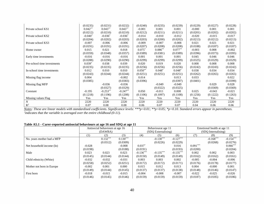
40

(0.0235) (0.0231) (0.0232) (0.0240) (0.0235) (0.0239) (0.0229) (0.0227) (0.0228)

Private school KS1 0.042** 0.043** 0.043** -0.001 0.001 0.001 -0.000 0.001 0.001

(0.0212) (0.0210) (0.0210) (0.0212) (0.0211) (0.0211) (0.0201) (0.0202) (0.0202)

Private school KS2 -0.040* -0.036* -0.036* -0.014 -0.010 -0.012 -0.020 -0.015 -0.017

(0.0204) (0.0202) (0.0203) (0.0203) (0.0200) (0.0202) (0.0213) (0.0212) (0.0213)

Private school KS3 -0.007 -0.006 -0.006 -0.009 -0.007 -0.008 0.021 0.021 0.021

(0.0191) (0.0191) (0.0191) (0.0207) (0.0208) (0.0208) (0.0188) (0.0187) (0.0187)

Home owner 0.015 0.021 0.018 0.075* 0.086** 0.077** -0.003 0.008 -0.002

(0.0359) (0.0348) (0.0357) (0.0389) (0.0381) (0.0389) (0.0396) (0.0373) (0.0395)

Early time investments -0.016 -0.016 -0.016 0.001 0.001 0.001 0.045 0.046 0.046

(0.0288) (0.0290) (0.0290) (0.0299) (0.0299) (0.0299) (0.0325) (0.0329) (0.0329)

Pre-school time investments 0.039* 0.038 0.039 0.020 0.019 0.020 0.008 0.008 0.008

(0.0235) (0.0235) (0.0235) (0.0256) (0.0256) (0.0256) (0.0242) (0.0243) (0.0242)

In-school time investments 0.012 0.010 0.010 0.050** 0.048* 0.048* 0.038 0.034 0.034

(0.0243) (0.0244) (0.0244) (0.0251) (0.0251) (0.0251) (0.0262) (0.0265) (0.0265)

Missing flag income 0.004 -0.002 0.014 0.013 0.033 0.022

(0.0385) (0.0383) (0.0396) (0.0397) (0.0401) (0.0399)

Missing flag MFP -0.036 -0.036 -0.049 -0.049 0.029 0.028

(0.0327) (0.0329) (0.0322) (0.0325) (0.0369) (0.0369)

Constant -0.195 -0.253** -0.247** 0.050 -0.011 0.008 0.025 -0.043 -0.021

(0.1218) (0.1196) (0.1208) (0.1106) (0.1097) (0.1108) (0.1256) (0.1222) (0.1263)

Missing values Flag Yes Yes Yes Yes Yes Yes Yes Yes Yes

N 2220 2220 2220 2220 2220 2220 2220 2220 2220

R2 0.07 0.08 0.08 0.06 0.07 0.07 0.04 0.06 0.06

Notes: These are linear models with standardised coefficients. Significance levels: ***p<0.01; **p<0.05; *p<0.10. Standard errors appear in parentheses. †indicates that the variable is averaged over the entire childhood (0-11).

Table A5.1 - Carer-reported antisocial behaviours at age 16 and SDQ at age 11 Antisocial behaviours at age 16

(DAWBA)

Behaviourat age 11

(SDQ Externalising)

Emotional health at age 11

(SDQ Internalising)

(1) (2) (3) (4) (5) (6) (7) (8) (9)

No. years mother had a MFP 0.132*** 0.130*** -0.130*** -0.127*** -0.168*** -0.154***

(0.0312) (0.0309) (0.0226) (0.0229) (0.0268) (0.0276)

Net household income (ln) -0.028 -0.008 0.037* 0.016 0.091*** 0.066***

(0.0198) (0.0188) (0.0191) (0.0193) (0.0200) (0.0204)

Male 0.023 0.023 0.023 -0.136*** -0.135*** -0.135*** 0.002 0.002 0.003

(0.0145) (0.0144) (0.0144) (0.0150) (0.0149) (0.0149) (0.0162) (0.0162) (0.0161)

Child ethnicity (White) -0.032 -0.032 -0.031 0.003 0.003 0.002 -0.005 -0.004 -0.006

(0.0258) (0.0252) (0.0251) (0.0172) (0.0172) (0.0171) (0.0176) (0.0178) (0.0177)

Mother not born in Europe -0.002 0.001 0.000 0.015 0.012 0.013 0.004 -0.000 0.001

(0.0149) (0.0144) (0.0145) (0.0137) (0.0137) (0.0138) (0.0148) (0.0146) (0.0147)

First born -0.018 -0.015 -0.015 -0.004 -0.008 -0.007 -0.022 -0.025 -0.026

(0.0146) (0.0145) (0.0146) (0.0159) (0.0159) (0.0159) (0.0187) (0.0185) (0.0186)

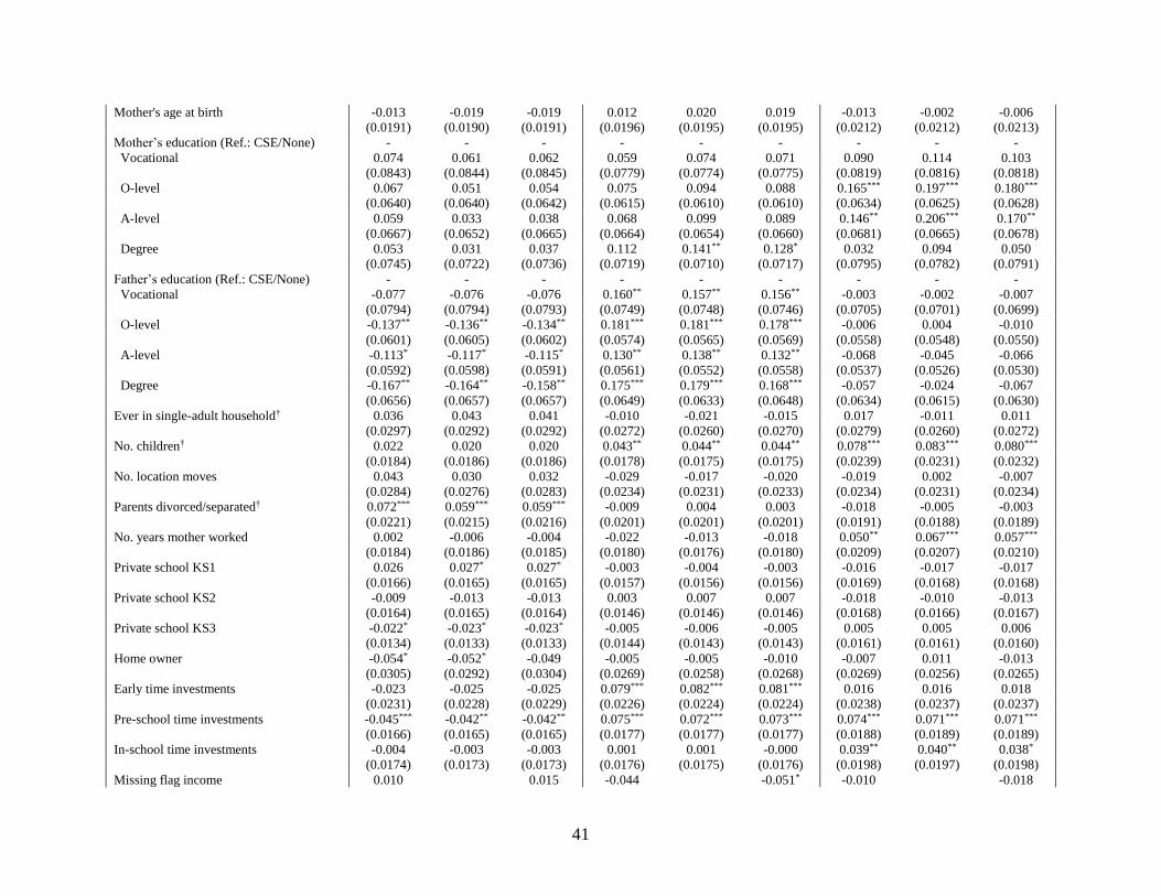
41

Mother's age at birth -0.013 -0.019 -0.019 0.012 0.020 0.019 -0.013 -0.002 -0.006

(0.0191) (0.0190) (0.0191) (0.0196) (0.0195) (0.0195) (0.0212) (0.0212) (0.0213)

Mother’s education (Ref.: CSE/None) - - - - - - - - -

Vocational 0.074 0.061 0.062 0.059 0.074 0.071 0.090 0.114 0.103

(0.0843) (0.0844) (0.0845) (0.0779) (0.0774) (0.0775) (0.0819) (0.0816) (0.0818)

O-level 0.067 0.051 0.054 0.075 0.094 0.088 0.165*** 0.197*** 0.180***

(0.0640) (0.0640) (0.0642) (0.0615) (0.0610) (0.0610) (0.0634) (0.0625) (0.0628)

A-level 0.059 0.033 0.038 0.068 0.099 0.089 0.146** 0.206*** 0.170**

(0.0667) (0.0652) (0.0665) (0.0664) (0.0654) (0.0660) (0.0681) (0.0665) (0.0678)

Degree 0.053 0.031 0.037 0.112 0.141** 0.128* 0.032 0.094 0.050

(0.0745) (0.0722) (0.0736) (0.0719) (0.0710) (0.0717) (0.0795) (0.0782) (0.0791)

Father’s education (Ref.: CSE/None) - - - - - - - - -

Vocational -0.077 -0.076 -0.076 0.160** 0.157** 0.156** -0.003 -0.002 -0.007

(0.0794) (0.0794) (0.0793) (0.0749) (0.0748) (0.0746) (0.0705) (0.0701) (0.0699)

O-level -0.137** -0.136** -0.134** 0.181*** 0.181*** 0.178*** -0.006 0.004 -0.010

(0.0601) (0.0605) (0.0602) (0.0574) (0.0565) (0.0569) (0.0558) (0.0548) (0.0550)

A-level -0.113* -0.117* -0.115* 0.130** 0.138** 0.132** -0.068 -0.045 -0.066

(0.0592) (0.0598) (0.0591) (0.0561) (0.0552) (0.0558) (0.0537) (0.0526) (0.0530)

Degree -0.167** -0.164** -0.158** 0.175*** 0.179*** 0.168*** -0.057 -0.024 -0.067

(0.0656) (0.0657) (0.0657) (0.0649) (0.0633) (0.0648) (0.0634) (0.0615) (0.0630)

Ever in single-adult household† 0.036 0.043 0.041 -0.010 -0.021 -0.015 0.017 -0.011 0.011

(0.0297) (0.0292) (0.0292) (0.0272) (0.0260) (0.0270) (0.0279) (0.0260) (0.0272)

No. children† 0.022 0.020 0.020 0.043** 0.044** 0.044** 0.078*** 0.083*** 0.080***

(0.0184) (0.0186) (0.0186) (0.0178) (0.0175) (0.0175) (0.0239) (0.0231) (0.0232)

No. location moves 0.043 0.030 0.032 -0.029 -0.017 -0.020 -0.019 0.002 -0.007

(0.0284) (0.0276) (0.0283) (0.0234) (0.0231) (0.0233) (0.0234) (0.0231) (0.0234)

Parents divorced/separated† 0.072*** 0.059*** 0.059*** -0.009 0.004 0.003 -0.018 -0.005 -0.003

(0.0221) (0.0215) (0.0216) (0.0201) (0.0201) (0.0201) (0.0191) (0.0188) (0.0189)

No. years mother worked 0.002 -0.006 -0.004 -0.022 -0.013 -0.018 0.050** 0.067*** 0.057***

(0.0184) (0.0186) (0.0185) (0.0180) (0.0176) (0.0180) (0.0209) (0.0207) (0.0210)

Private school KS1 0.026 0.027* 0.027* -0.003 -0.004 -0.003 -0.016 -0.017 -0.017

(0.0166) (0.0165) (0.0165) (0.0157) (0.0156) (0.0156) (0.0169) (0.0168) (0.0168)

Private school KS2 -0.009 -0.013 -0.013 0.003 0.007 0.007 -0.018 -0.010 -0.013

(0.0164) (0.0165) (0.0164) (0.0146) (0.0146) (0.0146) (0.0168) (0.0166) (0.0167)

Private school KS3 -0.022* -0.023* -0.023* -0.005 -0.006 -0.005 0.005 0.005 0.006

(0.0134) (0.0133) (0.0133) (0.0144) (0.0143) (0.0143) (0.0161) (0.0161) (0.0160)

Home owner -0.054* -0.052* -0.049 -0.005 -0.005 -0.010 -0.007 0.011 -0.013

(0.0305) (0.0292) (0.0304) (0.0269) (0.0258) (0.0268) (0.0269) (0.0256) (0.0265)

Early time investments -0.023 -0.025 -0.025 0.079*** 0.082*** 0.081*** 0.016 0.016 0.018

(0.0231) (0.0228) (0.0229) (0.0226) (0.0224) (0.0224) (0.0238) (0.0237) (0.0237)

Pre-school time investments -0.045*** -0.042** -0.042** 0.075*** 0.072*** 0.073*** 0.074*** 0.071*** 0.071***

(0.0166) (0.0165) (0.0165) (0.0177) (0.0177) (0.0177) (0.0188) (0.0189) (0.0189)

In-school time investments -0.004 -0.003 -0.003 0.001 0.001 -0.000 0.039** 0.040** 0.038*

(0.0174) (0.0173) (0.0173) (0.0176) (0.0175) (0.0176) (0.0198) (0.0197) (0.0198)

Missing flag income 0.010 0.015 -0.044 -0.051* -0.010 -0.018

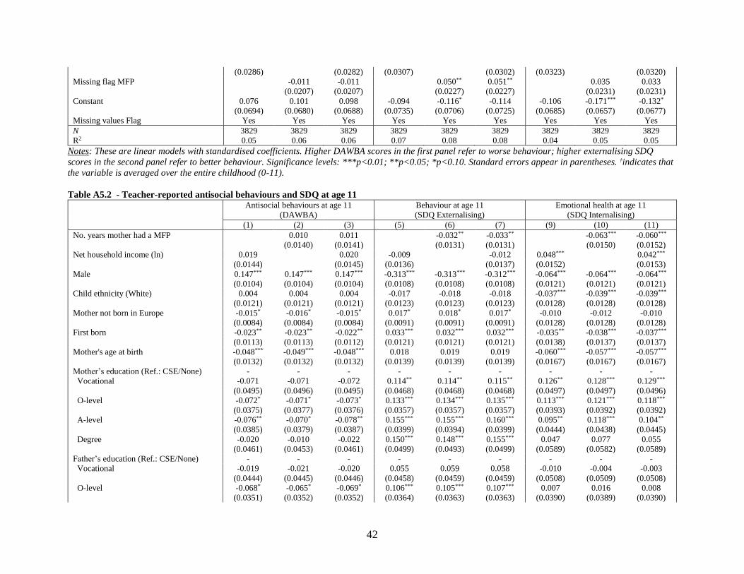
42

(0.0286) (0.0282) (0.0307) (0.0302) (0.0323) (0.0320)

Missing flag MFP -0.011 -0.011 0.050** 0.051** 0.035 0.033

(0.0207) (0.0207) (0.0227) (0.0227) (0.0231) (0.0231)

Constant 0.076 0.101 0.098 -0.094 -0.116* -0.114 -0.106 -0.171*** -0.132*

(0.0694) (0.0680) (0.0688) (0.0735) (0.0706) (0.0725) (0.0685) (0.0657) (0.0677)

Missing values Flag Yes Yes Yes Yes Yes Yes Yes Yes Yes

N 3829 3829 3829 3829 3829 3829 3829 3829 3829

R2 0.05 0.06 0.06 0.07 0.08 0.08 0.04 0.05 0.05

Notes: These are linear models with standardised coefficients. Higher DAWBA scores in the first panel refer to worse behaviour; higher externalising SDQ

scores in the second panel refer to better behaviour. Significance levels: ***p<0.01; **p<0.05; *p<0.10. Standard errors appear in parentheses. †indicates that

the variable is averaged over the entire childhood (0-11).

Table A5.2 - Teacher-reported antisocial behaviours and SDQ at age 11 Antisocial behaviours at age 11

(DAWBA)

Behaviour at age 11

(SDQ Externalising)

Emotional health at age 11

(SDQ Internalising)

(1) (2) (3) (5) (6) (7) (9) (10) (11)

No. years mother had a MFP 0.010 0.011 -0.032** -0.033** -0.063*** -0.060***

(0.0140) (0.0141) (0.0131) (0.0131) (0.0150) (0.0152)

Net household income (ln) 0.019 0.020 -0.009 -0.012 0.048*** 0.042***

(0.0144) (0.0145) (0.0136) (0.0137) (0.0152) (0.0153)

Male 0.147*** 0.147*** 0.147*** -0.313*** -0.313*** -0.312*** -0.064*** -0.064*** -0.064***

(0.0104) (0.0104) (0.0104) (0.0108) (0.0108) (0.0108) (0.0121) (0.0121) (0.0121)

Child ethnicity (White) 0.004 0.004 0.004 -0.017 -0.018 -0.018 -0.037*** -0.039*** -0.039***

(0.0121) (0.0121) (0.0121) (0.0123) (0.0123) (0.0123) (0.0128) (0.0128) (0.0128)

Mother not born in Europe -0.015* -0.016* -0.015* 0.017* 0.018* 0.017* -0.010 -0.012 -0.010

(0.0084) (0.0084) (0.0084) (0.0091) (0.0091) (0.0091) (0.0128) (0.0128) (0.0128)

First born -0.023** -0.023** -0.022** 0.033*** 0.032*** 0.032*** -0.035** -0.038*** -0.037***

(0.0113) (0.0113) (0.0112) (0.0121) (0.0121) (0.0121) (0.0138) (0.0137) (0.0137)

Mother's age at birth -0.048*** -0.049*** -0.048*** 0.018 0.019 0.019 -0.060*** -0.057*** -0.057***

(0.0132) (0.0132) (0.0132) (0.0139) (0.0139) (0.0139) (0.0167) (0.0167) (0.0167)

Mother’s education (Ref.: CSE/None) - - - - - - - - -

Vocational -0.071 -0.071 -0.072 0.114** 0.114** 0.115** 0.126** 0.128*** 0.129***

(0.0495) (0.0496) (0.0495) (0.0468) (0.0468) (0.0468) (0.0497) (0.0497) (0.0496)

O-level -0.072* -0.071* -0.073* 0.133*** 0.134*** 0.135*** 0.113*** 0.121*** 0.118***

(0.0375) (0.0377) (0.0376) (0.0357) (0.0357) (0.0357) (0.0393) (0.0392) (0.0392)

A-level -0.076** -0.070* -0.078** 0.155*** 0.155*** 0.160*** 0.095** 0.118*** 0.104**

(0.0385) (0.0379) (0.0387) (0.0399) (0.0394) (0.0399) (0.0444) (0.0438) (0.0445)

Degree -0.020 -0.010 -0.022 0.150*** 0.148*** 0.155*** 0.047 0.077 0.055

(0.0461) (0.0453) (0.0461) (0.0499) (0.0493) (0.0499) (0.0589) (0.0582) (0.0589)

Father’s education (Ref.: CSE/None) - - - - - - - - -

Vocational -0.019 -0.021 -0.020 0.055 0.059 0.058 -0.010 -0.004 -0.003

(0.0444) (0.0445) (0.0446) (0.0458) (0.0459) (0.0459) (0.0508) (0.0509) (0.0508)

O-level -0.068* -0.065* -0.069* 0.106*** 0.105*** 0.107*** 0.007 0.016 0.008

(0.0351) (0.0352) (0.0352) (0.0364) (0.0363) (0.0363) (0.0390) (0.0389) (0.0390)

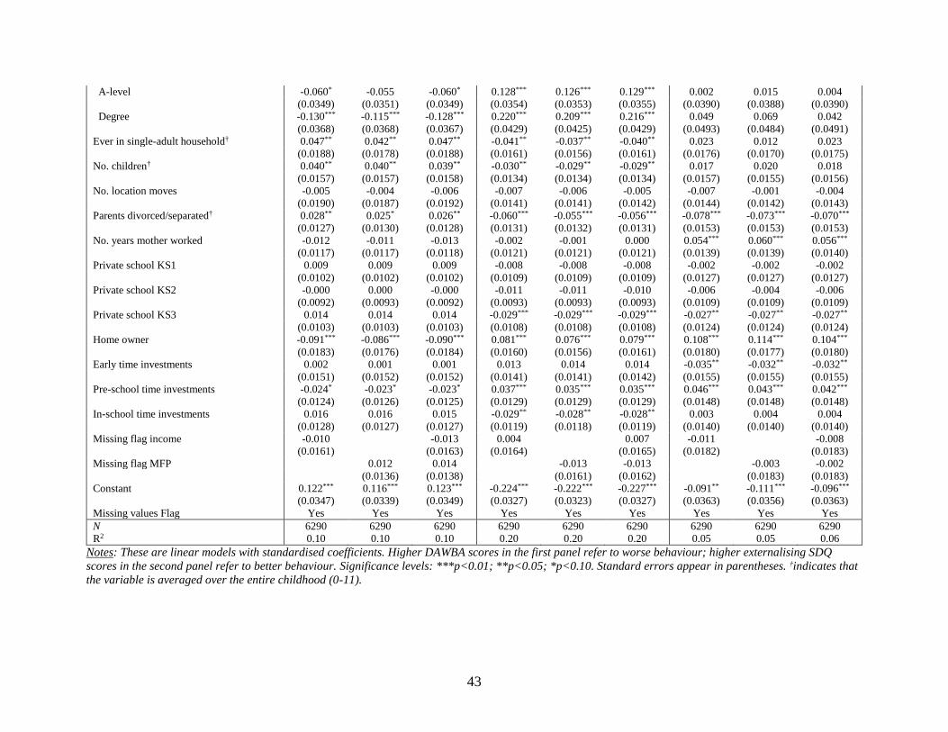
43

A-level -0.060* -0.055 -0.060* 0.128*** 0.126*** 0.129*** 0.002 0.015 0.004

(0.0349) (0.0351) (0.0349) (0.0354) (0.0353) (0.0355) (0.0390) (0.0388) (0.0390)

Degree -0.130*** -0.115*** -0.128*** 0.220*** 0.209*** 0.216*** 0.049 0.069 0.042

(0.0368) (0.0368) (0.0367) (0.0429) (0.0425) (0.0429) (0.0493) (0.0484) (0.0491)

Ever in single-adult household† 0.047** 0.042** 0.047** -0.041** -0.037** -0.040** 0.023 0.012 0.023

(0.0188) (0.0178) (0.0188) (0.0161) (0.0156) (0.0161) (0.0176) (0.0170) (0.0175)

No. children† 0.040** 0.040** 0.039** -0.030** -0.029** -0.029** 0.017 0.020 0.018

(0.0157) (0.0157) (0.0158) (0.0134) (0.0134) (0.0134) (0.0157) (0.0155) (0.0156)

No. location moves -0.005 -0.004 -0.006 -0.007 -0.006 -0.005 -0.007 -0.001 -0.004

(0.0190) (0.0187) (0.0192) (0.0141) (0.0141) (0.0142) (0.0144) (0.0142) (0.0143)

Parents divorced/separated† 0.028** 0.025* 0.026** -0.060*** -0.055*** -0.056*** -0.078*** -0.073*** -0.070***

(0.0127) (0.0130) (0.0128) (0.0131) (0.0132) (0.0131) (0.0153) (0.0153) (0.0153)

No. years mother worked -0.012 -0.011 -0.013 -0.002 -0.001 0.000 0.054*** 0.060*** 0.056***

(0.0117) (0.0117) (0.0118) (0.0121) (0.0121) (0.0121) (0.0139) (0.0139) (0.0140)

Private school KS1 0.009 0.009 0.009 -0.008 -0.008 -0.008 -0.002 -0.002 -0.002

(0.0102) (0.0102) (0.0102) (0.0109) (0.0109) (0.0109) (0.0127) (0.0127) (0.0127)

Private school KS2 -0.000 0.000 -0.000 -0.011 -0.011 -0.010 -0.006 -0.004 -0.006

(0.0092) (0.0093) (0.0092) (0.0093) (0.0093) (0.0093) (0.0109) (0.0109) (0.0109)

Private school KS3 0.014 0.014 0.014 -0.029*** -0.029*** -0.029*** -0.027** -0.027** -0.027**

(0.0103) (0.0103) (0.0103) (0.0108) (0.0108) (0.0108) (0.0124) (0.0124) (0.0124)

Home owner -0.091*** -0.086*** -0.090*** 0.081*** 0.076*** 0.079*** 0.108*** 0.114*** 0.104***

(0.0183) (0.0176) (0.0184) (0.0160) (0.0156) (0.0161) (0.0180) (0.0177) (0.0180)

Early time investments 0.002 0.001 0.001 0.013 0.014 0.014 -0.035** -0.032** -0.032**

(0.0151) (0.0152) (0.0152) (0.0141) (0.0141) (0.0142) (0.0155) (0.0155) (0.0155)

Pre-school time investments -0.024* -0.023* -0.023* 0.037*** 0.035*** 0.035*** 0.046*** 0.043*** 0.042***

(0.0124) (0.0126) (0.0125) (0.0129) (0.0129) (0.0129) (0.0148) (0.0148) (0.0148)

In-school time investments 0.016 0.016 0.015 -0.029** -0.028** -0.028** 0.003 0.004 0.004

(0.0128) (0.0127) (0.0127) (0.0119) (0.0118) (0.0119) (0.0140) (0.0140) (0.0140)

Missing flag income -0.010 -0.013 0.004 0.007 -0.011 -0.008

(0.0161) (0.0163) (0.0164) (0.0165) (0.0182) (0.0183)

Missing flag MFP 0.012 0.014 -0.013 -0.013 -0.003 -0.002

(0.0136) (0.0138) (0.0161) (0.0162) (0.0183) (0.0183)

Constant 0.122*** 0.116*** 0.123*** -0.224*** -0.222*** -0.227*** -0.091** -0.111*** -0.096***

(0.0347) (0.0339) (0.0349) (0.0327) (0.0323) (0.0327) (0.0363) (0.0356) (0.0363)

Missing values Flag Yes Yes Yes Yes Yes Yes Yes Yes Yes

N 6290 6290 6290 6290 6290 6290 6290 6290 6290

R2 0.10 0.10 0.10 0.20 0.20 0.20 0.05 0.05 0.06

Notes: These are linear models with standardised coefficients. Higher DAWBA scores in the first panel refer to worse behaviour; higher externalising SDQ

scores in the second panel refer to better behaviour. Significance levels: ***p<0.01; **p<0.05; *p<0.10. Standard errors appear in parentheses. †indicates that

the variable is averaged over the entire childhood (0-11).

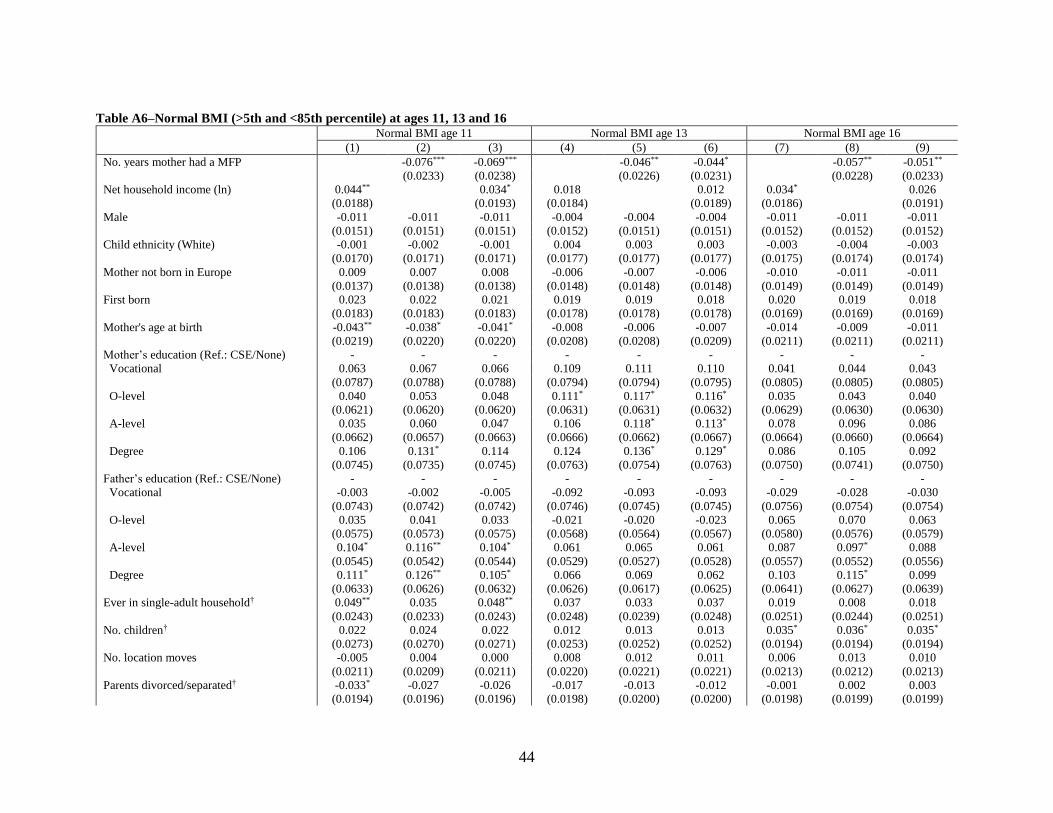
44

Table A6–Normal BMI (>5th and <85th percentile) at ages 11, 13 and 16 Normal BMI age 11 Normal BMI age 13 Normal BMI age 16

(1) (2) (3) (4) (5) (6) (7) (8) (9)

No. years mother had a MFP -0.076*** -0.069*** -0.046** -0.044* -0.057** -0.051**

(0.0233) (0.0238) (0.0226) (0.0231) (0.0228) (0.0233)

Net household income (ln) 0.044** 0.034* 0.018 0.012 0.034* 0.026

(0.0188) (0.0193) (0.0184) (0.0189) (0.0186) (0.0191)

Male -0.011 -0.011 -0.011 -0.004 -0.004 -0.004 -0.011 -0.011 -0.011

(0.0151) (0.0151) (0.0151) (0.0152) (0.0151) (0.0151) (0.0152) (0.0152) (0.0152)

Child ethnicity (White) -0.001 -0.002 -0.001 0.004 0.003 0.003 -0.003 -0.004 -0.003

(0.0170) (0.0171) (0.0171) (0.0177) (0.0177) (0.0177) (0.0175) (0.0174) (0.0174)

Mother not born in Europe 0.009 0.007 0.008 -0.006 -0.007 -0.006 -0.010 -0.011 -0.011

(0.0137) (0.0138) (0.0138) (0.0148) (0.0148) (0.0148) (0.0149) (0.0149) (0.0149)

First born 0.023 0.022 0.021 0.019 0.019 0.018 0.020 0.019 0.018

(0.0183) (0.0183) (0.0183) (0.0178) (0.0178) (0.0178) (0.0169) (0.0169) (0.0169)

Mother's age at birth -0.043** -0.038* -0.041* -0.008 -0.006 -0.007 -0.014 -0.009 -0.011

(0.0219) (0.0220) (0.0220) (0.0208) (0.0208) (0.0209) (0.0211) (0.0211) (0.0211)

Mother’s education (Ref.: CSE/None) - - - - - - - - -

Vocational 0.063 0.067 0.066 0.109 0.111 0.110 0.041 0.044 0.043

(0.0787) (0.0788) (0.0788) (0.0794) (0.0794) (0.0795) (0.0805) (0.0805) (0.0805)

O-level 0.040 0.053 0.048 0.111* 0.117* 0.116* 0.035 0.043 0.040

(0.0621) (0.0620) (0.0620) (0.0631) (0.0631) (0.0632) (0.0629) (0.0630) (0.0630)

A-level 0.035 0.060 0.047 0.106 0.118* 0.113* 0.078 0.096 0.086

(0.0662) (0.0657) (0.0663) (0.0666) (0.0662) (0.0667) (0.0664) (0.0660) (0.0664)

Degree 0.106 0.131* 0.114 0.124 0.136* 0.129* 0.086 0.105 0.092

(0.0745) (0.0735) (0.0745) (0.0763) (0.0754) (0.0763) (0.0750) (0.0741) (0.0750)

Father’s education (Ref.: CSE/None) - - - - - - - - -

Vocational -0.003 -0.002 -0.005 -0.092 -0.093 -0.093 -0.029 -0.028 -0.030

(0.0743) (0.0742) (0.0742) (0.0746) (0.0745) (0.0745) (0.0756) (0.0754) (0.0754)

O-level 0.035 0.041 0.033 -0.021 -0.020 -0.023 0.065 0.070 0.063

(0.0575) (0.0573) (0.0575) (0.0568) (0.0564) (0.0567) (0.0580) (0.0576) (0.0579)

A-level 0.104* 0.116** 0.104* 0.061 0.065 0.061 0.087 0.097* 0.088

(0.0545) (0.0542) (0.0544) (0.0529) (0.0527) (0.0528) (0.0557) (0.0552) (0.0556)

Degree 0.111* 0.126** 0.105* 0.066 0.069 0.062 0.103 0.115* 0.099

(0.0633) (0.0626) (0.0632) (0.0626) (0.0617) (0.0625) (0.0641) (0.0627) (0.0639)

Ever in single-adult household† 0.049** 0.035 0.048** 0.037 0.033 0.037 0.019 0.008 0.018

(0.0243) (0.0233) (0.0243) (0.0248) (0.0239) (0.0248) (0.0251) (0.0244) (0.0251)

No. children† 0.022 0.024 0.022 0.012 0.013 0.013 0.035* 0.036* 0.035*

(0.0273) (0.0270) (0.0271) (0.0253) (0.0252) (0.0252) (0.0194) (0.0194) (0.0194)

No. location moves -0.005 0.004 0.000 0.008 0.012 0.011 0.006 0.013 0.010

(0.0211) (0.0209) (0.0211) (0.0220) (0.0221) (0.0221) (0.0213) (0.0212) (0.0213)

Parents divorced/separated† -0.033* -0.027 -0.026 -0.017 -0.013 -0.012 -0.001 0.002 0.003

(0.0194) (0.0196) (0.0196) (0.0198) (0.0200) (0.0200) (0.0198) (0.0199) (0.0199)

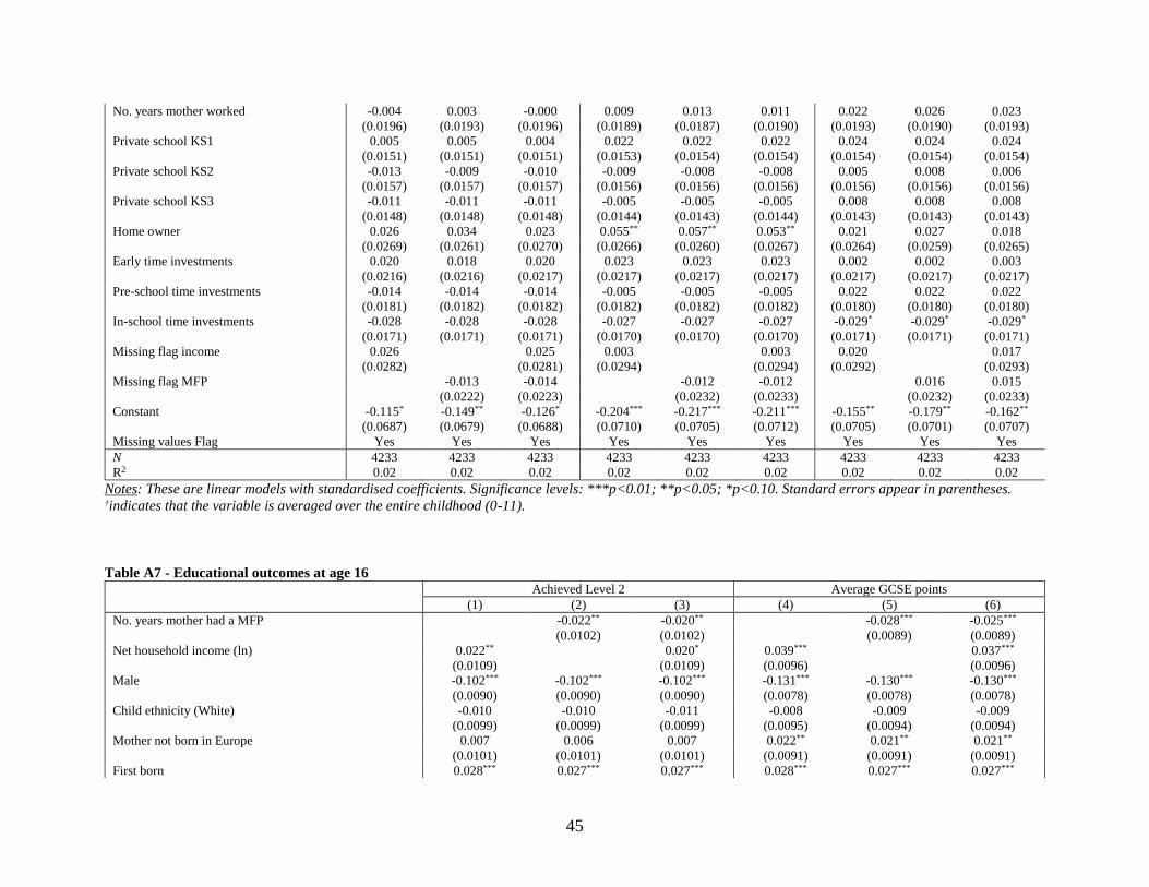
45

No. years mother worked -0.004 0.003 -0.000 0.009 0.013 0.011 0.022 0.026 0.023

(0.0196) (0.0193) (0.0196) (0.0189) (0.0187) (0.0190) (0.0193) (0.0190) (0.0193)

Private school KS1 0.005 0.005 0.004 0.022 0.022 0.022 0.024 0.024 0.024

(0.0151) (0.0151) (0.0151) (0.0153) (0.0154) (0.0154) (0.0154) (0.0154) (0.0154)

Private school KS2 -0.013 -0.009 -0.010 -0.009 -0.008 -0.008 0.005 0.008 0.006

(0.0157) (0.0157) (0.0157) (0.0156) (0.0156) (0.0156) (0.0156) (0.0156) (0.0156)

Private school KS3 -0.011 -0.011 -0.011 -0.005 -0.005 -0.005 0.008 0.008 0.008

(0.0148) (0.0148) (0.0148) (0.0144) (0.0143) (0.0144) (0.0143) (0.0143) (0.0143)

Home owner 0.026 0.034 0.023 0.055** 0.057** 0.053** 0.021 0.027 0.018

(0.0269) (0.0261) (0.0270) (0.0266) (0.0260) (0.0267) (0.0264) (0.0259) (0.0265)

Early time investments 0.020 0.018 0.020 0.023 0.023 0.023 0.002 0.002 0.003

(0.0216) (0.0216) (0.0217) (0.0217) (0.0217) (0.0217) (0.0217) (0.0217) (0.0217)

Pre-school time investments -0.014 -0.014 -0.014 -0.005 -0.005 -0.005 0.022 0.022 0.022

(0.0181) (0.0182) (0.0182) (0.0182) (0.0182) (0.0182) (0.0180) (0.0180) (0.0180)

In-school time investments -0.028 -0.028 -0.028 -0.027 -0.027 -0.027 -0.029* -0.029* -0.029*

(0.0171) (0.0171) (0.0171) (0.0170) (0.0170) (0.0170) (0.0171) (0.0171) (0.0171)

Missing flag income 0.026 0.025 0.003 0.003 0.020 0.017

(0.0282) (0.0281) (0.0294) (0.0294) (0.0292) (0.0293)

Missing flag MFP -0.013 -0.014 -0.012 -0.012 0.016 0.015

(0.0222) (0.0223) (0.0232) (0.0233) (0.0232) (0.0233)

Constant -0.115* -0.149** -0.126* -0.204*** -0.217*** -0.211*** -0.155** -0.179** -0.162**

(0.0687) (0.0679) (0.0688) (0.0710) (0.0705) (0.0712) (0.0705) (0.0701) (0.0707)

Missing values Flag Yes Yes Yes Yes Yes Yes Yes Yes Yes

N 4233 4233 4233 4233 4233 4233 4233 4233 4233

R2 0.02 0.02 0.02 0.02 0.02 0.02 0.02 0.02 0.02

Notes: These are linear models with standardised coefficients. Significance levels: ***p<0.01; **p<0.05; *p<0.10. Standard errors appear in parentheses. †indicates that the variable is averaged over the entire childhood (0-11).

Table A7 - Educational outcomes at age 16 Achieved Level 2 Average GCSE points

(1) (2) (3) (4) (5) (6)

No. years mother had a MFP -0.022** -0.020** -0.028*** -0.025***

(0.0102) (0.0102) (0.0089) (0.0089)

Net household income (ln) 0.022** 0.020* 0.039*** 0.037***

(0.0109) (0.0109) (0.0096) (0.0096)

Male -0.102*** -0.102*** -0.102*** -0.131*** -0.130*** -0.130***

(0.0090) (0.0090) (0.0090) (0.0078) (0.0078) (0.0078)

Child ethnicity (White) -0.010 -0.010 -0.011 -0.008 -0.009 -0.009

(0.0099) (0.0099) (0.0099) (0.0095) (0.0094) (0.0094)

Mother not born in Europe 0.007 0.006 0.007 0.022** 0.021** 0.021**

(0.0101) (0.0101) (0.0101) (0.0091) (0.0091) (0.0091)

First born 0.028*** 0.027*** 0.027*** 0.028*** 0.027*** 0.027***

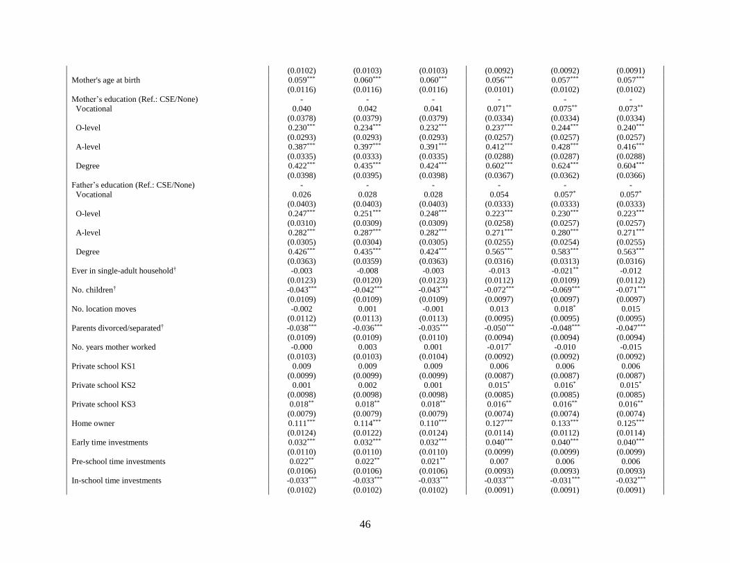
46

(0.0102) (0.0103) (0.0103) (0.0092) (0.0092) (0.0091)

Mother's age at birth 0.059*** 0.060*** 0.060*** 0.056*** 0.057*** 0.057***

(0.0116) (0.0116) (0.0116) (0.0101) (0.0102) (0.0102)

Mother’s education (Ref.: CSE/None) - - - - - -

Vocational 0.040 0.042 0.041 0.071** 0.075** 0.073**

(0.0378) (0.0379) (0.0379) (0.0334) (0.0334) (0.0334)

O-level 0.230*** 0.234*** 0.232*** 0.237*** 0.244*** 0.240***

(0.0293) (0.0293) (0.0293) (0.0257) (0.0257) (0.0257)

A-level 0.387*** 0.397*** 0.391*** 0.412*** 0.428*** 0.416***

(0.0335) (0.0333) (0.0335) (0.0288) (0.0287) (0.0288)

Degree 0.422*** 0.435*** 0.424*** 0.602*** 0.624*** 0.604***

(0.0398) (0.0395) (0.0398) (0.0367) (0.0362) (0.0366)

Father’s education (Ref.: CSE/None) - - - - - -

Vocational 0.026 0.028 0.028 0.054 0.057* 0.057*

(0.0403) (0.0403) (0.0403) (0.0333) (0.0333) (0.0333)

O-level 0.247*** 0.251*** 0.248*** 0.223*** 0.230*** 0.223***

(0.0310) (0.0309) (0.0309) (0.0258) (0.0257) (0.0257)

A-level 0.282*** 0.287*** 0.282*** 0.271*** 0.280*** 0.271***

(0.0305) (0.0304) (0.0305) (0.0255) (0.0254) (0.0255)

Degree 0.426*** 0.435*** 0.424*** 0.565*** 0.583*** 0.563***

(0.0363) (0.0359) (0.0363) (0.0316) (0.0313) (0.0316)

Ever in single-adult household† -0.003 -0.008 -0.003 -0.013 -0.021** -0.012

(0.0123) (0.0120) (0.0123) (0.0112) (0.0109) (0.0112)

No. children† -0.043*** -0.042*** -0.043*** -0.072*** -0.069*** -0.071***

(0.0109) (0.0109) (0.0109) (0.0097) (0.0097) (0.0097)

No. location moves -0.002 0.001 -0.001 0.013 0.018* 0.015

(0.0112) (0.0113) (0.0113) (0.0095) (0.0095) (0.0095)

Parents divorced/separated† -0.038*** -0.036*** -0.035*** -0.050*** -0.048*** -0.047***

(0.0109) (0.0109) (0.0110) (0.0094) (0.0094) (0.0094)

No. years mother worked -0.000 0.003 0.001 -0.017* -0.010 -0.015

(0.0103) (0.0103) (0.0104) (0.0092) (0.0092) (0.0092)

Private school KS1 0.009 0.009 0.009 0.006 0.006 0.006

(0.0099) (0.0099) (0.0099) (0.0087) (0.0087) (0.0087)

Private school KS2 0.001 0.002 0.001 0.015* 0.016* 0.015*

(0.0098) (0.0098) (0.0098) (0.0085) (0.0085) (0.0085)

Private school KS3 0.018** 0.018** 0.018** 0.016** 0.016** 0.016**

(0.0079) (0.0079) (0.0079) (0.0074) (0.0074) (0.0074)

Home owner 0.111*** 0.114*** 0.110*** 0.127*** 0.133*** 0.125***

(0.0124) (0.0122) (0.0124) (0.0114) (0.0112) (0.0114)

Early time investments 0.032*** 0.032*** 0.032*** 0.040*** 0.040*** 0.040***

(0.0110) (0.0110) (0.0110) (0.0099) (0.0099) (0.0099)

Pre-school time investments 0.022** 0.022** 0.021** 0.007 0.006 0.006

(0.0106) (0.0106) (0.0106) (0.0093) (0.0093) (0.0093)

In-school time investments -0.033*** -0.033*** -0.033*** -0.033*** -0.031*** -0.032***

(0.0102) (0.0102) (0.0102) (0.0091) (0.0091) (0.0091)

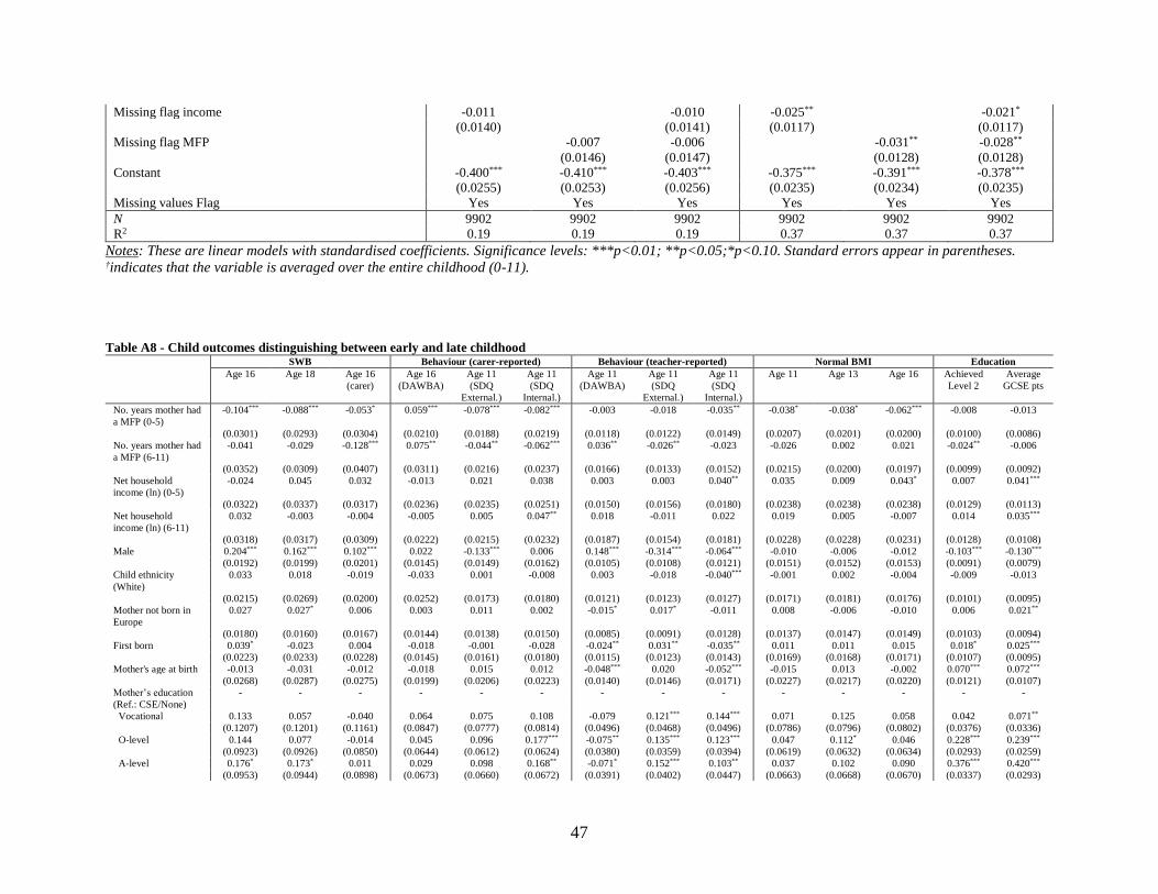
47

Missing flag income -0.011 -0.010 -0.025** -0.021*

(0.0140) (0.0141) (0.0117) (0.0117)

Missing flag MFP -0.007 -0.006 -0.031** -0.028**

(0.0146) (0.0147) (0.0128) (0.0128)

Constant -0.400*** -0.410*** -0.403*** -0.375*** -0.391*** -0.378***

(0.0255) (0.0253) (0.0256) (0.0235) (0.0234) (0.0235)

Missing values Flag Yes Yes Yes Yes Yes Yes

N 9902 9902 9902 9902 9902 9902

R2 0.19 0.19 0.19 0.37 0.37 0.37

Notes: These are linear models with standardised coefficients. Significance levels: ***p<0.01; **p<0.05;*p<0.10. Standard errors appear in parentheses. †indicates that the variable is averaged over the entire childhood (0-11).

Table A8 - Child outcomes distinguishing between early and late childhood

SWB Behaviour (carer-reported) Behaviour (teacher-reported) Normal BMI Education

Age 16 Age 18 Age 16

(carer)

Age 16

(DAWBA)

Age 11

(SDQ

External.)

Age 11

(SDQ

Internal.)

Age 11

(DAWBA)

Age 11

(SDQ

External.)

Age 11

(SDQ

Internal.)

Age 11 Age 13 Age 16 Achieved

Level 2

Average

GCSE pts

No. years mother had

a MFP (0-5)

-0.104*** -0.088*** -0.053* 0.059*** -0.078*** -0.082*** -0.003 -0.018 -0.035** -0.038* -0.038* -0.062*** -0.008 -0.013

(0.0301) (0.0293) (0.0304) (0.0210) (0.0188) (0.0219) (0.0118) (0.0122) (0.0149) (0.0207) (0.0201) (0.0200) (0.0100) (0.0086)

No. years mother had

a MFP (6-11)

-0.041 -0.029 -0.128*** 0.075** -0.044** -0.062*** 0.036** -0.026** -0.023 -0.026 0.002 0.021 -0.024** -0.006

(0.0352) (0.0309) (0.0407) (0.0311) (0.0216) (0.0237) (0.0166) (0.0133) (0.0152) (0.0215) (0.0200) (0.0197) (0.0099) (0.0092)

Net household

income (ln) (0-5)

-0.024 0.045 0.032 -0.013 0.021 0.038 0.003 0.003 0.040** 0.035 0.009 0.043* 0.007 0.041***

(0.0322) (0.0337) (0.0317) (0.0236) (0.0235) (0.0251) (0.0150) (0.0156) (0.0180) (0.0238) (0.0238) (0.0238) (0.0129) (0.0113)

Net household

income (ln) (6-11)

0.032 -0.003 -0.004 -0.005 0.005 0.047** 0.018 -0.011 0.022 0.019 0.005 -0.007 0.014 0.035***

(0.0318) (0.0317) (0.0309) (0.0222) (0.0215) (0.0232) (0.0187) (0.0154) (0.0181) (0.0228) (0.0228) (0.0231) (0.0128) (0.0108)

Male 0.204*** 0.162*** 0.102*** 0.022 -0.133*** 0.006 0.148*** -0.314*** -0.064*** -0.010 -0.006 -0.012 -0.103*** -0.130***

(0.0192) (0.0199) (0.0201) (0.0145) (0.0149) (0.0162) (0.0105) (0.0108) (0.0121) (0.0151) (0.0152) (0.0153) (0.0091) (0.0079)

Child ethnicity

(White)

0.033 0.018 -0.019 -0.033 0.001 -0.008 0.003 -0.018 -0.040*** -0.001 0.002 -0.004 -0.009 -0.013

(0.0215) (0.0269) (0.0200) (0.0252) (0.0173) (0.0180) (0.0121) (0.0123) (0.0127) (0.0171) (0.0181) (0.0176) (0.0101) (0.0095)

Mother not born in

Europe

0.027 0.027* 0.006 0.003 0.011 0.002 -0.015* 0.017* -0.011 0.008 -0.006 -0.010 0.006 0.021**

(0.0180) (0.0160) (0.0167) (0.0144) (0.0138) (0.0150) (0.0085) (0.0091) (0.0128) (0.0137) (0.0147) (0.0149) (0.0103) (0.0094)

First born 0.039* -0.023 0.004 -0.018 -0.001 -0.028 -0.024** 0.031** -0.035** 0.011 0.011 0.015 0.018* 0.025***

(0.0223) (0.0233) (0.0228) (0.0145) (0.0161) (0.0180) (0.0115) (0.0123) (0.0143) (0.0169) (0.0168) (0.0171) (0.0107) (0.0095)

Mother's age at birth -0.013 -0.031 -0.012 -0.018 0.015 0.012 -0.048*** 0.020 -0.052*** -0.015 0.013 -0.002 0.070*** 0.072***

(0.0268) (0.0287) (0.0275) (0.0199) (0.0206) (0.0223) (0.0140) (0.0146) (0.0171) (0.0227) (0.0217) (0.0220) (0.0121) (0.0107)

Mother’s education

(Ref.: CSE/None)

- - - - - - - - - - - - - -

Vocational 0.133 0.057 -0.040 0.064 0.075 0.108 -0.079 0.121*** 0.144*** 0.071 0.125 0.058 0.042 0.071**

(0.1207) (0.1201) (0.1161) (0.0847) (0.0777) (0.0814) (0.0496) (0.0468) (0.0496) (0.0786) (0.0796) (0.0802) (0.0376) (0.0336)

O-level 0.144 0.077 -0.014 0.045 0.096 0.177*** -0.075** 0.135*** 0.123*** 0.047 0.112* 0.046 0.228*** 0.239***

(0.0923) (0.0926) (0.0850) (0.0644) (0.0612) (0.0624) (0.0380) (0.0359) (0.0394) (0.0619) (0.0632) (0.0634) (0.0293) (0.0259)

A-level 0.176* 0.173* 0.011 0.029 0.098 0.168** -0.071* 0.152*** 0.103** 0.037 0.102 0.090 0.376*** 0.420***

(0.0953) (0.0944) (0.0898) (0.0673) (0.0660) (0.0672) (0.0391) (0.0402) (0.0447) (0.0663) (0.0668) (0.0670) (0.0337) (0.0293)

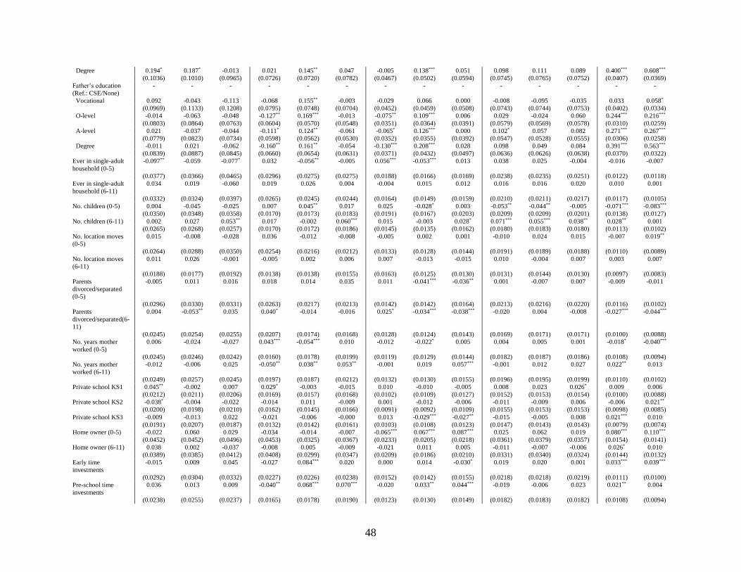
48

Degree 0.194* 0.187* -0.013 0.021 0.145** 0.047 -0.005 0.138*** 0.051 0.098 0.111 0.089 0.400*** 0.608***

(0.1036) (0.1010) (0.0965) (0.0726) (0.0720) (0.0782) (0.0467) (0.0502) (0.0594) (0.0745) (0.0765) (0.0752) (0.0407) (0.0369)

Father’s education

(Ref.: CSE/None)

- - - - - - - - - - - - - -

Vocational 0.092 -0.043 -0.113 -0.068 0.155** -0.003 -0.029 0.066 0.000 -0.008 -0.095 -0.035 0.033 0.058*

(0.0969) (0.1133) (0.1208) (0.0795) (0.0748) (0.0704) (0.0452) (0.0459) (0.0508) (0.0743) (0.0744) (0.0753) (0.0402) (0.0334)

O-level -0.014 -0.063 -0.048 -0.127** 0.169*** -0.013 -0.075** 0.109*** 0.006 0.029 -0.024 0.060 0.244*** 0.216***

(0.0803) (0.0864) (0.0763) (0.0604) (0.0570) (0.0548) (0.0351) (0.0364) (0.0391) (0.0579) (0.0569) (0.0578) (0.0310) (0.0259)

A-level 0.021 -0.037 -0.044 -0.111* 0.124** -0.061 -0.065* 0.126*** 0.000 0.102* 0.057 0.082 0.271*** 0.267***

(0.0779) (0.0823) (0.0734) (0.0598) (0.0562) (0.0530) (0.0352) (0.0355) (0.0392) (0.0547) (0.0528) (0.0555) (0.0306) (0.0258)

Degree -0.011 0.021 -0.062 -0.160** 0.161** -0.054 -0.130*** 0.208*** 0.028 0.098 0.049 0.084 0.391*** 0.563***

(0.0839) (0.0887) (0.0845) (0.0660) (0.0654) (0.0631) (0.0371) (0.0432) (0.0497) (0.0636) (0.0626) (0.0638) (0.0370) (0.0322)

Ever in single-adult

household (0-5)

-0.097** -0.059 -0.077* 0.032 -0.056** -0.005 0.056*** -0.053*** 0.013 0.038 0.025 -0.004 -0.016 -0.007

(0.0377) (0.0366) (0.0465) (0.0296) (0.0275) (0.0275) (0.0188) (0.0166) (0.0169) (0.0238) (0.0235) (0.0251) (0.0122) (0.0118)

Ever in single-adult

household (6-11)

0.034 0.019 -0.060 0.019 0.026 0.004 -0.004 0.015 0.012 0.016 0.016 0.020 0.010 0.001

(0.0332) (0.0324) (0.0397) (0.0265) (0.0245) (0.0244) (0.0164) (0.0149) (0.0159) (0.0210) (0.0211) (0.0217) (0.0117) (0.0105)

No. children (0-5) 0.004 -0.045 -0.025 0.007 0.045** 0.017 0.025 -0.028* 0.003 -0.053** -0.044** -0.005 -0.071*** -0.083***

(0.0350) (0.0348) (0.0358) (0.0170) (0.0173) (0.0183) (0.0191) (0.0167) (0.0203) (0.0209) (0.0209) (0.0201) (0.0138) (0.0127)

No. children (6-11) 0.002 0.027 0.053** 0.017 -0.002 0.060*** 0.015 -0.003 0.028* 0.071*** 0.055*** 0.038** 0.028** 0.001

(0.0265) (0.0268) (0.0257) (0.0170) (0.0172) (0.0186) (0.0145) (0.0135) (0.0162) (0.0180) (0.0183) (0.0180) (0.0113) (0.0102)

No. location moves

(0-5)

0.015 -0.008 -0.028 0.036 -0.012 -0.008 -0.005 0.002 0.001 -0.010 0.024 0.015 -0.007 0.019**

(0.0264) (0.0288) (0.0350) (0.0254) (0.0216) (0.0212) (0.0133) (0.0128) (0.0144) (0.0191) (0.0189) (0.0188) (0.0110) (0.0089)

No. location moves

(6-11)

0.011 0.026 -0.001 -0.005 0.002 0.006 0.007 -0.013 -0.015 0.010 -0.004 0.007 0.003 0.007

(0.0188) (0.0177) (0.0192) (0.0138) (0.0138) (0.0155) (0.0163) (0.0125) (0.0130) (0.0131) (0.0144) (0.0130) (0.0097) (0.0083)

Parents

divorced/separated

(0-5)

-0.005 0.011 0.016 0.018 0.014 0.035 0.011 -0.041*** -0.036** 0.001 -0.007 0.007 -0.009 -0.011

(0.0296) (0.0330) (0.0331) (0.0263) (0.0217) (0.0213) (0.0142) (0.0142) (0.0164) (0.0213) (0.0216) (0.0220) (0.0116) (0.0102)

Parents

divorced/separated(6-

11)

0.004 -0.053** 0.035 0.040* -0.014 -0.016 0.025* -0.034*** -0.038*** -0.020 0.004 -0.008 -0.027*** -0.044***

(0.0245) (0.0254) (0.0255) (0.0207) (0.0174) (0.0168) (0.0128) (0.0124) (0.0143) (0.0169) (0.0171) (0.0171) (0.0100) (0.0088)

No. years mother

worked (0-5)

0.006 -0.024 -0.027 0.043*** -0.054*** 0.010 -0.012 -0.022* 0.005 0.004 0.005 0.001 -0.018* -0.040***

(0.0245) (0.0246) (0.0242) (0.0160) (0.0178) (0.0199) (0.0119) (0.0129) (0.0144) (0.0182) (0.0187) (0.0186) (0.0108) (0.0094)

No. years mother

worked (6-11)

-0.012 -0.006 0.025 -0.050** 0.038** 0.053** -0.001 0.019 0.057*** -0.001 0.012 0.027 0.022** 0.013

(0.0249) (0.0257) (0.0245) (0.0197) (0.0187) (0.0212) (0.0132) (0.0130) (0.0155) (0.0196) (0.0195) (0.0199) (0.0110) (0.0102)

Private school KS1 0.045** -0.002 0.007 0.029* -0.003 -0.015 0.010 -0.010 -0.005 0.008 0.023 0.026* 0.009 0.006

(0.0212) (0.0211) (0.0206) (0.0169) (0.0157) (0.0168) (0.0102) (0.0109) (0.0127) (0.0152) (0.0153) (0.0154) (0.0100) (0.0088)

Private school KS2 -0.038* -0.004 -0.022 -0.014 0.011 -0.009 0.001 -0.012 -0.006 -0.011 -0.009 0.006 -0.006 0.021**

(0.0200) (0.0198) (0.0210) (0.0162) (0.0145) (0.0166) (0.0091) (0.0092) (0.0109) (0.0155) (0.0153) (0.0153) (0.0098) (0.0085)

Private school KS3 -0.009 -0.013 0.022 -0.021 -0.006 -0.000 0.013 -0.029*** -0.027** -0.015 -0.005 0.008 0.021*** 0.010

(0.0191) (0.0207) (0.0187) (0.0132) (0.0142) (0.0161) (0.0103) (0.0108) (0.0123) (0.0147) (0.0143) (0.0143) (0.0079) (0.0074)

Home owner (0-5) -0.022 0.060 0.029 -0.034 -0.014 -0.007 -0.065*** 0.067*** 0.087*** 0.025 0.062 0.019 0.080*** 0.110***

(0.0452) (0.0452) (0.0496) (0.0453) (0.0325) (0.0367) (0.0233) (0.0205) (0.0218) (0.0361) (0.0379) (0.0357) (0.0154) (0.0141)

Home owner (6-11) 0.038 0.002 -0.037 -0.008 0.005 -0.009 -0.021 0.011 0.005 -0.011 -0.007 -0.006 0.026* 0.010

(0.0389) (0.0385) (0.0412) (0.0408) (0.0299) (0.0347) (0.0209) (0.0186) (0.0210) (0.0331) (0.0340) (0.0324) (0.0144) (0.0132)

Early time

investments

-0.015 0.009 0.045 -0.027 0.084*** 0.020 0.000 0.014 -0.030* 0.019 0.020 0.001 0.033*** 0.039***

(0.0292) (0.0304) (0.0332) (0.0227) (0.0226) (0.0238) (0.0152) (0.0142) (0.0155) (0.0218) (0.0218) (0.0219) (0.0111) (0.0100)

Pre-school time

investments

0.036 0.013 0.009 -0.040** 0.068*** 0.070*** -0.020 0.033** 0.044*** -0.019 -0.006 0.023 0.021** 0.004

(0.0238) (0.0255) (0.0237) (0.0165) (0.0178) (0.0190) (0.0123) (0.0130) (0.0149) (0.0182) (0.0183) (0.0182) (0.0108) (0.0094)

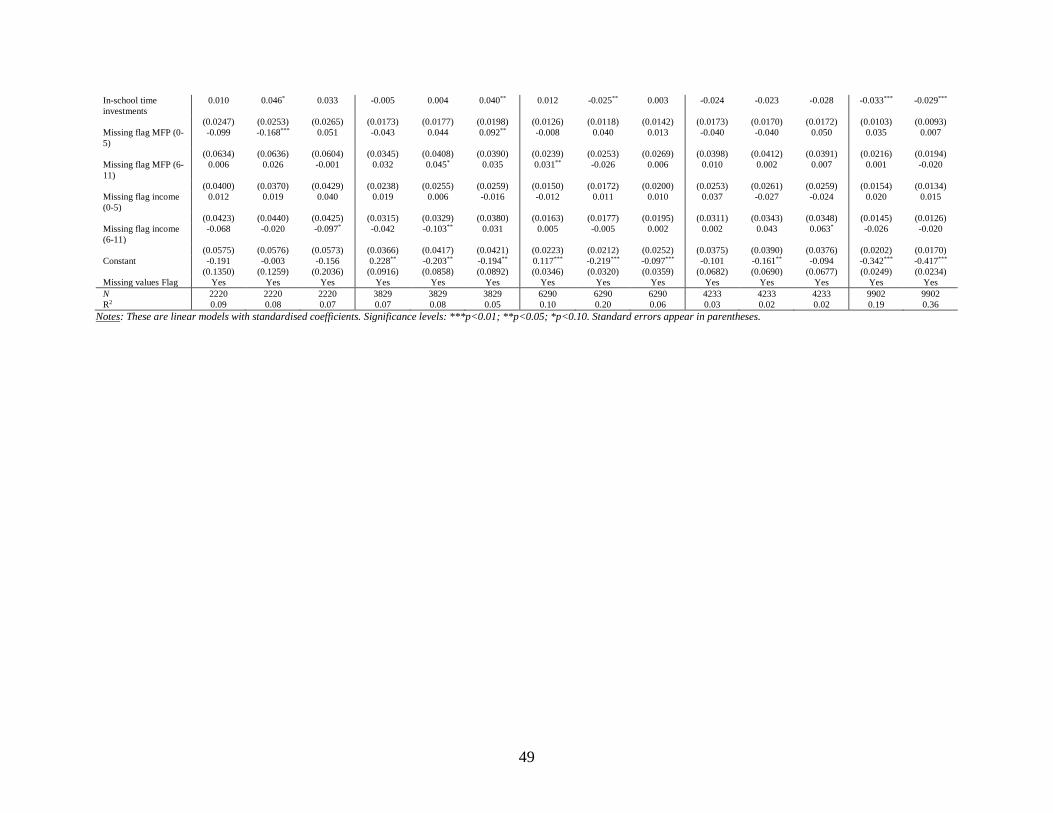
49

In-school time

investments

0.010 0.046* 0.033 -0.005 0.004 0.040** 0.012 -0.025** 0.003 -0.024 -0.023 -0.028 -0.033*** -0.029***

(0.0247) (0.0253) (0.0265) (0.0173) (0.0177) (0.0198) (0.0126) (0.0118) (0.0142) (0.0173) (0.0170) (0.0172) (0.0103) (0.0093)

Missing flag MFP (0-

5)

-0.099 -0.168*** 0.051 -0.043 0.044 0.092** -0.008 0.040 0.013 -0.040 -0.040 0.050 0.035 0.007

(0.0634) (0.0636) (0.0604) (0.0345) (0.0408) (0.0390) (0.0239) (0.0253) (0.0269) (0.0398) (0.0412) (0.0391) (0.0216) (0.0194)

Missing flag MFP (6-

11)

0.006 0.026 -0.001 0.032 0.045* 0.035 0.031** -0.026 0.006 0.010 0.002 0.007 0.001 -0.020

(0.0400) (0.0370) (0.0429) (0.0238) (0.0255) (0.0259) (0.0150) (0.0172) (0.0200) (0.0253) (0.0261) (0.0259) (0.0154) (0.0134)

Missing flag income

(0-5)

0.012 0.019 0.040 0.019 0.006 -0.016 -0.012 0.011 0.010 0.037 -0.027 -0.024 0.020 0.015

(0.0423) (0.0440) (0.0425) (0.0315) (0.0329) (0.0380) (0.0163) (0.0177) (0.0195) (0.0311) (0.0343) (0.0348) (0.0145) (0.0126)

Missing flag income

(6-11)

-0.068 -0.020 -0.097* -0.042 -0.103** 0.031 0.005 -0.005 0.002 0.002 0.043 0.063* -0.026 -0.020

(0.0575) (0.0576) (0.0573) (0.0366) (0.0417) (0.0421) (0.0223) (0.0212) (0.0252) (0.0375) (0.0390) (0.0376) (0.0202) (0.0170)

Constant -0.191 -0.003 -0.156 0.228** -0.203** -0.194** 0.117*** -0.219*** -0.097*** -0.101 -0.161** -0.094 -0.342*** -0.417***

(0.1350) (0.1259) (0.2036) (0.0916) (0.0858) (0.0892) (0.0346) (0.0320) (0.0359) (0.0682) (0.0690) (0.0677) (0.0249) (0.0234)

Missing values Flag Yes Yes Yes Yes Yes Yes Yes Yes Yes Yes Yes Yes Yes Yes

N 2220 2220 2220 3829 3829 3829 6290 6290 6290 4233 4233 4233 9902 9902

R2 0.09 0.08 0.07 0.07 0.08 0.05 0.10 0.20 0.06 0.03 0.02 0.02 0.19 0.36

Notes: These are linear models with standardised coefficients. Significance levels: ***p<0.01; **p<0.05; *p<0.10. Standard errors appear in parentheses.

Appendix B – Questionnaires

B1. Major Financial Problems (MFP)

The question on major financial problem is part of a list of life events that could happen to the mother

since a certain age of the child. The question is: “Listed below are a number of events which may have

brought changes in your life. Have any of these occurred since your study child’s XXX birthday?” One of

these events is our variable of interest: “You had a major financial problem”. The question is asked at the

following child ages: 8 months, 1y9m, 2y9m, 3y11m, 5y1m, 6y1m, 9y2m, 11y2m.

In the first six waves (from 8m to 6y1m) the question asks whether the mother had a MFP and how

much she was affected by it. The possible answers are “Yes, and affected me a lot”, “Yes, moderately

affected”, “Yes, mildly affected”, “Yes, but didn’t affect me” and “No”. In the results reported in the main

text, we created a dummy variable for each wave taking value 1 if the mother reported to have had a MFP

(from Yes, affected a lot to Yes, but didn’t affect me). When possible (in the first six waves of ALSPAC

data), we have checked that the results are almost unchanged when recoding “Yes, but didn’t affect me” to

a value of 0 for the MFP dummy.

In the waves corresponding to child’s age 9y2m and 11y2m, the questions asks only whether a MFP

occurred, but it refers not only to the previous year but also to the last two years. Specifically the answers

to the question at age 9y2m are: “Yes, when the study child was 6 or 7”,“Yes, since the child’s 8th birthday”,

“Yes, both when the study child was 6/7 and 8+”, “No, didn’t happen in the past 3 years”. And similarly

at age 11y2m: “Yes, when the study child was 9 or 10”, “Yes, since the child’s 11th birthday”, “Yes, both

when the study child was 9/10 and 11+”, “No, didn’t happen in this period”. From the answer at age 9y2m

and 11y2m we can derive information on whether the mother had a MFP when the child was 6/7 and 9.

For each child’s age from 8 months to age 11 we have a dummy taking value 1 if the mother had a

MFP in the previous year (from child’s birth in the case of the questionnaire at 8 months). The final measure

of financial insecurity is the number of year from child’s birth to age 11 in which the mother reported a

MFP.

51

B2. Short Moods and Feeling Questionnaire (SMFQ)

These questions are about how you may have been feeling or acting recently. For each question, please say how

much you have felt or acted this way in the past two weeks.

In the past two weeks: NOT TRUE SOMETIMES TRUE

1. I felt miserable or unhappy. 2 1 0

2. I didn't enjoy anything at all. 2 1 0

3. I felt so tired I just sat around and did nothing. 2 1 0

4. I was very restless. 2 1 0

5. I felt I was no good anymore. 2 1 0

6. I cried a lot. 2 1 0

7. I found it hard to think properly or concentrate. 2 1 0

8. I hated myself. 2 1 0

9. I was a bad person. 2 1 0

10. I felt lonely. 2 1 0

11. I thought nobody really loved me. 2 1 0

12. I thought I could never be as good as other kids. 2 1 0

13. I felt I did everything wrong. 2 1 0

Total Subjective well-being score: 0-26

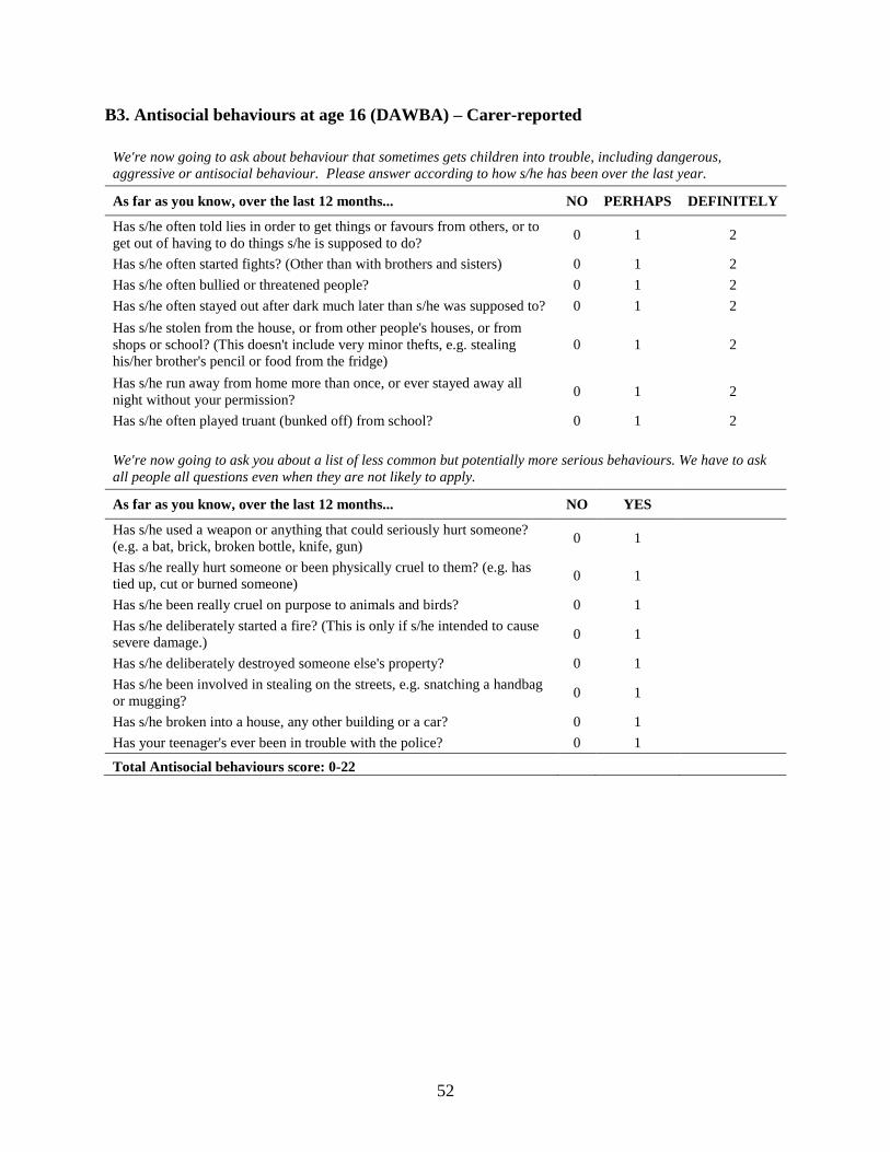
52

B3. Antisocial behaviours at age 16 (DAWBA) – Carer-reported

We're now going to ask about behaviour that sometimes gets children into trouble, including dangerous,

aggressive or antisocial behaviour. Please answer according to how s/he has been over the last year.

As far as you know, over the last 12 months... NO PERHAPS DEFINITELY

Has s/he often told lies in order to get things or favours from others, or to

get out of having to do things s/he is supposed to do? 0 1 2

Has s/he often started fights? (Other than with brothers and sisters) 0 1 2

Has s/he often bullied or threatened people? 0 1 2

Has s/he often stayed out after dark much later than s/he was supposed to? 0 1 2

Has s/he stolen from the house, or from other people's houses, or from

shops or school? (This doesn't include very minor thefts, e.g. stealing

his/her brother's pencil or food from the fridge)

0 1 2

Has s/he run away from home more than once, or ever stayed away all

night without your permission? 0 1 2

Has s/he often played truant (bunked off) from school? 0 1 2

We're now going to ask you about a list of less common but potentially more serious behaviours. We have to ask

all people all questions even when they are not likely to apply.

As far as you know, over the last 12 months... NO YES

Has s/he used a weapon or anything that could seriously hurt someone?

(e.g. a bat, brick, broken bottle, knife, gun) 0 1

Has s/he really hurt someone or been physically cruel to them? (e.g. has

tied up, cut or burned someone) 0 1

Has s/he been really cruel on purpose to animals and birds? 0 1

Has s/he deliberately started a fire? (This is only if s/he intended to cause

severe damage.) 0 1

Has s/he deliberately destroyed someone else's property? 0 1

Has s/he been involved in stealing on the streets, e.g. snatching a handbag

or mugging? 0 1

Has s/he broken into a house, any other building or a car? 0 1

Has your teenager's ever been in trouble with the police? 0 1

Total Antisocial behaviours score: 0-22

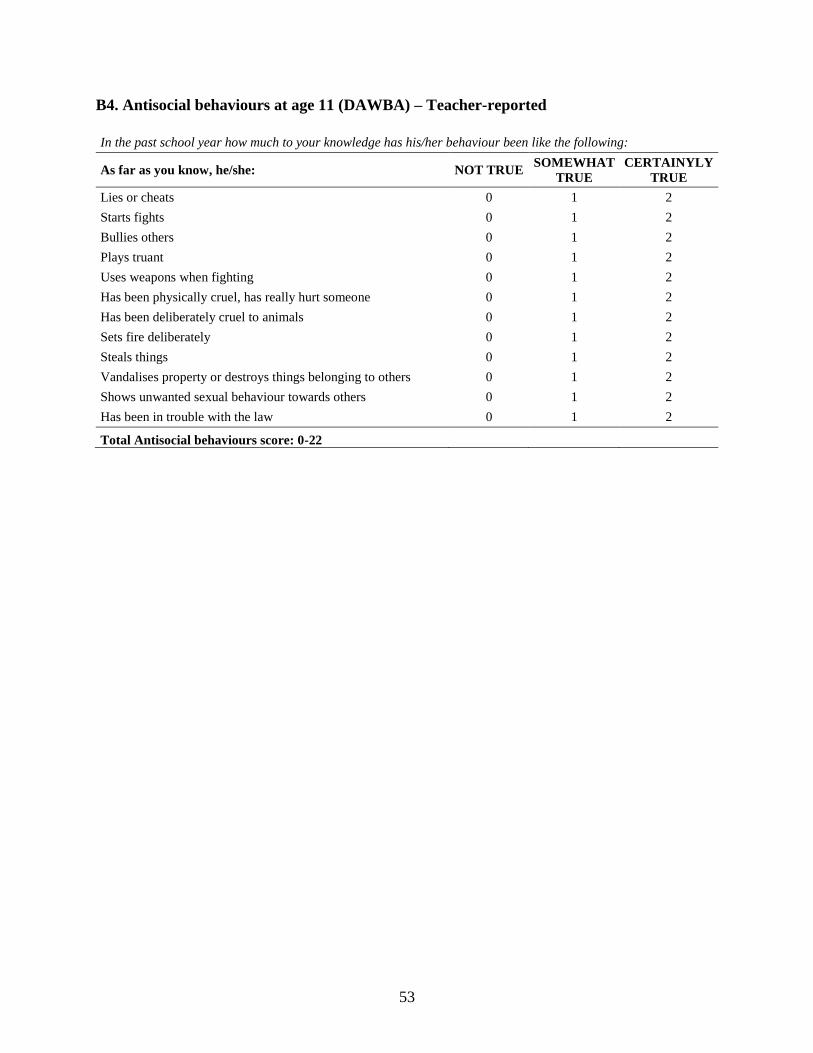
53

B4. Antisocial behaviours at age 11 (DAWBA) – Teacher-reported

In the past school year how much to your knowledge has his/her behaviour been like the following:

As far as you know, he/she: NOT TRUE SOMEWHAT

TRUE

CERTAINYLY

TRUE

Lies or cheats 0 1 2

Starts fights 0 1 2

Bullies others 0 1 2

Plays truant 0 1 2

Uses weapons when fighting 0 1 2

Has been physically cruel, has really hurt someone 0 1 2

Has been deliberately cruel to animals 0 1 2

Sets fire deliberately 0 1 2

Steals things 0 1 2

Vandalises property or destroys things belonging to others 0 1 2

Shows unwanted sexual behaviour towards others 0 1 2

Has been in trouble with the law 0 1 2

Total Antisocial behaviours score: 0-22

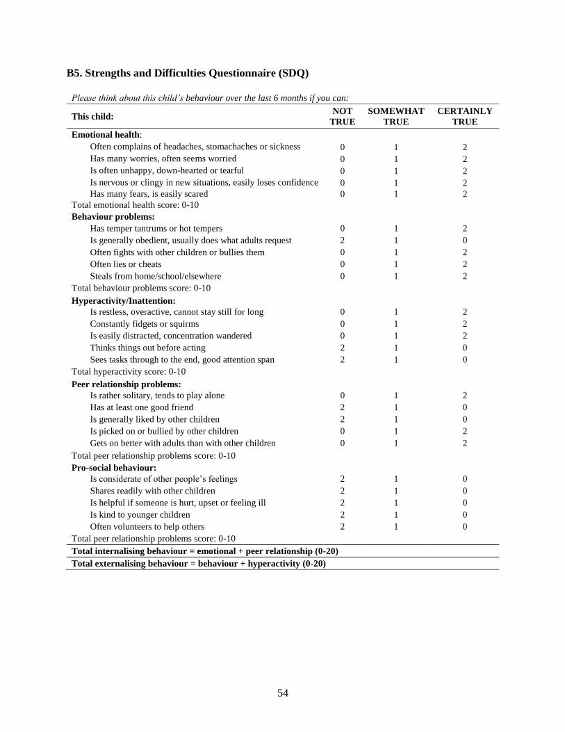
54

B5. Strengths and Difficulties Questionnaire (SDQ)

Please think about this child’s behaviour over the last 6 months if you can:

This child: NOT

TRUE

SOMEWHAT

TRUE

CERTAINLY

TRUE

Emotional health:

Often complains of headaches, stomachaches or sickness 0 1 2

Has many worries, often seems worried 0 1 2

Is often unhappy, down-hearted or tearful 0 1 2

Is nervous or clingy in new situations, easily loses confidence 0 1 2

Has many fears, is easily scared 0 1 2

Total emotional health score: 0-10

Behaviour problems:

Has temper tantrums or hot tempers 0 1 2

Is generally obedient, usually does what adults request 2 1 0

Often fights with other children or bullies them 0 1 2

Often lies or cheats 0 1 2

Steals from home/school/elsewhere 0 1 2

Total behaviour problems score: 0-10

Hyperactivity/Inattention:

Is restless, overactive, cannot stay still for long 0 1 2

Constantly fidgets or squirms 0 1 2

Is easily distracted, concentration wandered 0 1 2

Thinks things out before acting 2 1 0

Sees tasks through to the end, good attention span 2 1 0

Total hyperactivity score: 0-10

Peer relationship problems:

Is rather solitary, tends to play alone 0 1 2

Has at least one good friend 2 1 0

Is generally liked by other children 2 1 0

Is picked on or bullied by other children 0 1 2

Gets on better with adults than with other children 0 1 2

Total peer relationship problems score: 0-10

Pro-social behaviour:

Is considerate of other people’s feelings 2 1 0

Shares readily with other children 2 1 0

Is helpful if someone is hurt, upset or feeling ill 2 1 0

Is kind to younger children 2 1 0

Often volunteers to help others 2 1 0

Total peer relationship problems score: 0-10

Total internalising behaviour = emotional + peer relationship (0-20)

Total externalising behaviour = behaviour + hyperactivity (0-20)

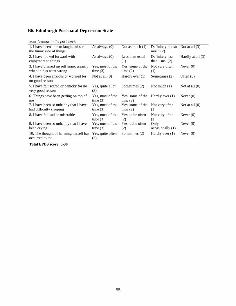
55

B6. Edinburgh Post-natal Depression Scale

Your feelings in the past week.

1. I have been able to laugh and see

the funny side of things

As always (0) Not as much (1) Definitely not so

much (2)

Not at all (3)

2. I have looked forward with

enjoyment to things

As always (0) Less than usual

(1)

Definitely less

than usual (2)

Hardly at all (3)

3. I have blamed myself unnecessarily

when things went wrong

Yes, most of the

time (3)

Yes, some of the

time (2)

Not very often

(1)

Never (0)

4. I have been anxious or worried for

no good reason

Not at all (0) Hardly ever (1) Sometimes (2) Often (3)

5. I have felt scared or panicky for no

very good reason

Yes, quite a lot

(3)

Sometimes (2) Not much (1) Not at all (0)

6. Things have been getting on top of

me

Yes, most of the

time (3)

Yes, some of the

time (2)

Hardly ever (1) Never (0)

7. I have been so unhappy that I have

had difficulty sleeping

Yes, most of the

time (3)

Yes, some of the

time (2)

Not very often

(1)

Not at all (0)

8. I have felt sad or miserable Yes, most of the

time (3)

Yes, quite often

(2)

Not very often

(1)

Never (0)

9. I have been so unhappy that I have

been crying

Yes, most of the

time (3)

Yes, quite often

(2)

Only

occasionally (1)

Never (0)

10. The thought of harming myself has

occurred to me

Yes, quite often

(3)

Sometimes (2) Hardly ever (1) Never (0)

Total EPDS score: 0-30

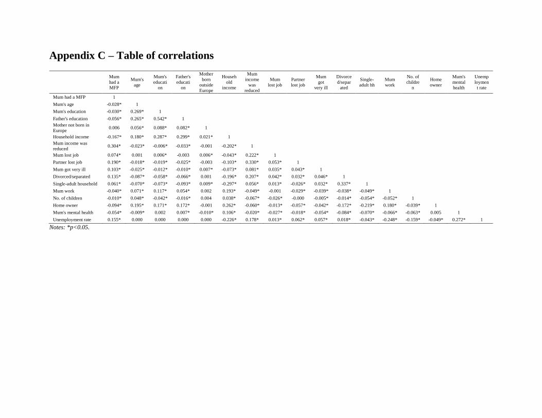
Appendix C – Table of correlations

Mum

had a

MFP

Mum's

age

Mum's

educati

on

Father's

educati

on

Mother

born

outside

Europe

Househ

old

income

Mum

income

was

reduced

Mum

lost job

Partner

lost job

Mum

got

very ill

Divorce

d/separ

ated

Single-

adult hh

Mum

work

No. of

childre

n

Home

owner

Mum's

mental

health

Unemp

loymen

t rate

Mum had a MFP 1

Mum's age -0.028* 1

Mum's education -0.030* 0.269* 1

Father's education -0.056* 0.265* 0.542* 1

Mother not born in

Europe 0.006 0.056* 0.088* 0.082* 1

Household income -0.167* 0.180* 0.287* 0.299* 0.021* 1

Mum income was

reduced 0.304* -0.023* -0.006* -0.033* -0.001 -0.202* 1

Mum lost job 0.074* 0.001 0.006* -0.003 0.006* -0.043* 0.222* 1

Partner lost job 0.190* -0.018* -0.019* -0.025* -0.003 -0.103* 0.330* 0.053* 1

Mum got very ill 0.103* -0.025* -0.012* -0.010* 0.007* -0.073* 0.081* 0.035* 0.043* 1

Divorced/separated 0.135* -0.087* -0.058* -0.066* 0.001 -0.196* 0.207* 0.042* 0.032* 0.046* 1

Single-adult household 0.061* -0.070* -0.073* -0.093* 0.009* -0.297* 0.056* 0.013* -0.026* 0.032* 0.337* 1

Mum work -0.040* 0.071* 0.117* 0.054* 0.002 0.193* -0.049* -0.001 -0.029* -0.039* -0.038* -0.049* 1

No. of children -0.010* 0.048* -0.042* -0.016* 0.004 0.038* -0.067* -0.026* -0.000 -0.005* -0.014* -0.054* -0.052* 1

Home owner -0.094* 0.195* 0.171* 0.172* -0.001 0.262* -0.060* -0.013* -0.057* -0.042* -0.172* -0.219* 0.180* -0.039* 1

Mum's mental health -0.054* -0.009* 0.002 0.007* -0.010* 0.106* -0.020* -0.027* -0.018* -0.054* -0.084* -0.070* -0.066* -0.063* 0.005 1

Unemployment rate 0.155* 0.000 0.000 0.000 0.000 -0.226* 0.178* 0.013* 0.062* 0.057* 0.018* -0.043* -0.248* -0.159* -0.049* 0.272* 1

Notes: *p<0.05.

CENTRE FOR ECONOMIC PERFORMANCE Recent Discussion Papers

1608 Boris Hirsch Elke J. Jahn Alan Manning Michael Oberfichtner

The Urban Wage Premium in Imperfect Labour Markets

1607 Max Nathan Anna Rosso

Innovative Events

1606 Christopher T. Stanton Catherine Thomas

Missing Trade in Tasks: Employer Outsourcing in the Gig Economy

1605 Jan-Emmanuel De Neve Christian Krekel George Ward

Employee Wellbeing, Productivity and Firm Performance

1604 Stephen Gibbons Cong Peng Cheng Keat Tang

Valuing the Environmental Benefits of Canals Using House Prices

1603 Mary Amiti Stephen J. Redding David Weinstein

The Impact of the 2018 Trade War on U.S. Prices and Welfare

1602 Greer Gosnell Ralf Martin Mirabelle Muûls Quentin Coutellier Goran Strbac Mingyang Sun Simon Tindermans

Making Smart Meters Smarter the Smart Way

1601 Antoine Dechezleprêtre Caterina Gennaioli Ralf Martin Mirabelle Muûls Thomas Stoerk

Searching for Carbon Leaks in Multinational Companies

1600 Jeremiah Dittmar Skipper Seabold

New Media and Competition: Printing and Europe's Transformation after Gutenberg

1599 Kilian Huber Volker Lindenthal Fabian Waldinger

Discrimination, Managers, and Firm Performance: Evidence from “Aryanizations” in Nazi Germany

1598 Julia Cajal-Grossi Rocco Macchiavello Guillermo Noguera

International Buyers’ Sourcing and Suppliers’ Markups in Bangladeshi Garments

1597 Alex Bell Raj Chetty Xavier Jaravel Neviana Petkova John Van Reenen

Do Tax Cuts Produce More Einsteins? The Impact of Financial Incentives vs. Exposure to Innovation on the Supply of Inventors

1596 Matthew Baird A.V. Chari Shanthi Nataraj Alexander Rothenberg Shqiponja Telhaj L. Alan Winters

The Public Sector and the Misallocation of Labor: Evidence from a Policy Experiment in India

1595 Stephen J. Redding David E. Weinstein

Aggregation and the Gravity Equation

1594 Andy Feng Anna Valero

Skill Based Management: Evidence from Manufacturing Firms

1593 Leonardo Baccini Giammario Impullitti Edmund J. Malesky

Globalization and State Capitalism: Assessing Vietnam's Accession to the WTO

The Centre for Economic Performance Publications Unit Tel: +44 (0)20 7955 7673 Email info@cep.lse.ac.uk Website: http://cep.lse.ac.uk Twitter: @CEP_LSE