ISSN 2042-2695

CEP Discussion Paper No 1520

December 2017

The Productivity Puzzle and Misallocation: An Italian Perspective

Sara Calligaris Massimo Del Gatto

Fadi Hassan Gianmarco I.P. Ottaviano

Fabiano Schivardi

Abstract Productivity has recently slowed down in many economies around the world. A crucial challenge in understanding what lies behind this “productivity puzzle” is the still short time span for which data can be analysed. An exception is Italy where productivity growth started to stagnate 25 years ago. Italy therefore offers an interesting case to investigate in search of broader lessons that may hold beyond local specific cities. We find that resource misallocation has played a sizeable role in slowing down Italian productivity growth. If misallocation had remained at its 1995 level, in 2013 Italy's aggregate productivity would have been 18% higher than its actual level. Misallocation has mainly risen within sectors than between them, increasing more in sectors where the world technological frontier has expanded faster. Relative specialization in those sectors explains the patterns of misallocation across geographical areas and firm size classes. The broader message is that an important part of the explanation of the productivity puzzle may lie in the rising difficulty of reallocating resources between firms in sectors where technology is changing faster rather than between sectors with different speeds of technological change.

Keywords: misallocation, TFP, productivity puzzle, Italy JEL: D22; D24; O11; O47

This paper was produced as part of the Centre’s Trade Programme. The Centre for Economic Performance is financed by the Economic and Social Research Council.

We thank Andrea Brandolini, Matteo Bugamelli, Sergio De Nardis, Lazaros Dimitriadis, Luigi Guiso, Silvia Fabiani, Francesca Lotti, Dino Pinelli, and Roberta Torre for useful comments and discussions. We thank the Directorate General for Economic and Financial Affairs (DG ECFIN) of the European Commission for financial support. The opinions expressed and arguments employed herein are those of the authors and do not necessarily reflect the official views of the OECD or of the governments of its member countries.

Sara Calligaris, OECD and EIEF. Massimo Del Gatto, G.d Annunzio University and CRENoS. Fadi Hassan, Trinity College Dublin, Centre for Economic Performance, London School of Economics and Bank of Italy. Gianmarco I.P. Ottaviano, London School of Economics, University Bocconi, Centre for Economic Performance, London School of Economics and CEPR. Fabiano Schivardi, LUISS, EIEF and CEPR.

Published by Centre for Economic Performance London School of Economics and Political Science Houghton Street London WC2A 2AE

All rights reserved. No part of this publication may be reproduced, stored in a retrieval system or transmitted in any form or by any means without the prior permission in writing of the publisher nor be issued to the public or circulated in any form other than that in which it is published.

Requests for permission to reproduce any article or part of the Working Paper should be sent to the editor at the above address.

S. Calligaris, M. Del Gatto, F. Hassan, G.I.P. Ottaviano and F. Schivardi, submitted 2017.

1 Introduction

In recent years, many advanced economies have experienced a serious productiv-

ity slowdown. As Figure 1 shows, in the US, the Eurozone and the UK total factor

productivity is still below the pre-global financial crisis level. In 2016, US labor pro-

ductivity growth fell into negative territory for the first time in the last three decades

(Conference Board, 2016) and productivity has reached the headlines of global me-

dia, which have started focusing on “The productivity puzzle that baffles the world’s

economies”.1 These trends are particularly worrisome because productivity lies at the

heart of long-term growth.

A crucial challenge in understanding what lies behind this productivity puzzle is

the still short time span for which data can be analysed. As Fernald (2014) and Cette

et al. (2016) point out, in some countries like the US, the productivity slowdown dates

back a few years before the crisis. However, in Italy this is a much longer standing

issue. Figure 2 shows a growth accounting decomposition for Italy over the past four

decades and the results are quite emblematic. TFP growth shrank throughout the

decades, becoming negative in the 2000s. Italy turned from being among the fastest

growing EU economies into the “sleeping beauty of Europe”, a country rich in talent

and history but suffering from a long-lasting stagnation (Hassan and Ottaviano, 2013).

TFP dynamics in the manufacturing sector, where measurement issues are less binding

than in services, captures well the timing of the Italian decline. Figure 3 shows a

dramatic slowdown in TFP growth since the mid-Nineties for Italy compared to France

and Germany, where TFP continued to grow up to the global financial crisis.2

The relatively long time-series dimension that characterises the Italian productiv-

ity slowdown makes Italy a relevant case-study for analysing the key features of the

productivity decline (and draw policy recommendations) that can be of general inter-

est to other countries. We analyse the firm-level dimension of aggregate productivity

and focus on the concept of resource “misalocation” and its impact on productivity.

The “productivity” we refer to is Total Factor Productivity (henceforth, simply TFP),

1The Financial Times, 29th May, 2016.2In the paper we focus on firms in the manufacturing sector, because firm-level TFP measurement

is less controversial than in services due to better accounting of the capital stock. We have run thesame analysis also for firms in the service sector and comparable results are quite similar.

2

which measures how effectively given amounts of productive factors (capital and labor)

are used. Clearly the economy’s aggregate TFP depends on its firms’ TFP. This hap-

pens along two dimensions. On the one hand, for given amounts of factors used by each

firm, aggregate TFP grows when individual firm TFP grows, for example thanks to

the adoption of better technologies and management practices. If market imperfections

prevent firms from seizing these opportunities, the economy’s productive apparatus is

exposed to obsolescence and senescence with adverse effects on aggregate TFP.

On the other hand, for given individual firm-level TFP, aggregate TFP depends

on how factors are allocated across firms. As long as market frictions “distort” the

allocation of product demand and factor supply away from high TFP firms towards low

TFP rivals, they lead to lower aggregate TFP than in an ideal situation of frictionless

markets. Building on the distinction, introduced by Foster et al. (2008), between

physical TFP (TFPQ or simply TFP, i.e., measured as the ability to generate physical

output from given inputs) and revenue TFP (TFPR, i.e., measured as the ability to

generate revenue from given inputs), Hsieh and Klenow (2009) construct a model of

monopolistic competition in which, although firms can differ in their physical TFP, in

the absence of frictions TFPR is the same for all firms. The idea behind this result is

simple: with no frictions, the marginal revenue product of inputs should be equalized

across firms as factors move from low to high marginal revenue product firms. As

marginal revenue product equalization implies TFPR equalization, Hsieh and Klenow

(2009) call deviations from a situation in which TFPR is equalized “misallocation”,

and propose a simple way to measure its consequences on aggregate TFP. This is also

the definition of “misallocation” we adopt. It implies that the dispersion of TFPR

across firms can be used to measure the extent of misallocation. It also implies that

firms with a TFPR higher than the sectoral average are inefficiently small, while those

with a TFPR below the sectoral average are inefficiently large. These are the two key

implications of the misallocation literature that we use in this paper.

With these definitions in mind, we study the universe of Italian incorporated com-

panies over the period 1993-2013 and find strong evidence of increased misallocation

since 1995. If misallocation had remained at its 1995 level, in 2013 aggregate TFP

would have been 18% higher than its current level. This would have translated into

1% higher GDP growth per-year, which would have helped to close the growth gap with

3

France and Germany. The main source of misallocation comes from the within industry

component rather than the between component: misallocation has mainly risen within

sectors than between them, increasing more in sectors where the world technological

frontier has expanded faster. Relative specialization in those sectors explains the pat-

terns of misallocation across geographical areas and firm size classes with misallocation

increasing particularly in the Northern regions and among big firms, which tradition-

ally are the driving forces of the Italian economy. The broader message is that an

important part of the explanation of the recent productivity puzzle may lie in a gener-

ally rising difficulty of reallocating resources between firms in sectors where technology

is changing faster rather than between sectors with different speeds of technological

change. This implies that moving factors of production from e.g. textile into IT would

increase aggregate productivity less than ensuring that the most efficient firms within

textile are the ones that absorb more resources.

In the wake of Griffith, Redding and Van Reenen (2004) we measure the speed

of technological change in a sector by the average change of R&D intensity between

1987-1993 and 1994-2007 in advanced countries.3 We find a positive and significant

correlation between the increase in R&D intensity in advanced countries and the in-

crease in misallocation in Italian sectors. Once we account for the sectoral composition

of Italian regions and firm size classes, the implied “frontier shocks” are the strongest

for Northern regions and big firms, thus matching the relative increase in misallocation

across geographical areas and firm sizes.

The analysis of firm characteristics associated with firms being inefficiently sized

sheds additional light on the relation between exposure to frontier shocks and misalloca-

tion within industries. In particular, we look at corporate ownership and management,

finance, workforce composition, internationalization and innovation. We find that firms

more likely to be keeping up with the technological frontier are inefficiently small and

thus under-resourced. These are the firms that employ a larger share of graduates and

invest more in intangible assets. On the contrary, firms less likely to be keeping up are

inefficiently large and thus over-resourced. These are the firms that have a large share

3R&D intensity is measured as the share of R&D expenditure over value added at the sectoral level.Data are from the ANBERD database of the OECD. We exclude Italy from the sample and, followingGriffith, Redding and Van Reenen (2004), the countries that we consider are Canada, Denmark,Finland, France, Germany, Japan, Netherlands, Norway, Sweden, United Kingdom, and United States.Results hold also when we take R&D intensity in the US only.

4

of workers under a wage supplementation scheme, that are family managed, and that

are financially constrained. We interpret this as evidence that rising within-industry

misallocation is consistent with an increase in the volatility of idiosyncratic shocks to

firms due to their heterogeneous ability to respond to sectoral “frontier shocks” in the

presence of sluggish reallocation of resources.

A concern with our quantification exercise relates to measurement error in firms’

revenues and inputs. As Bils et al. (2017) point out, mismeasurement is likely to distort

the misallocation analysis as a firm’s TFPR is higher when revenues are overstated

and/or inputs are understated: if, for example, the extent of revenue overstatement

(input understatement) systematically grows (falls) with firms’ true revenues (inputs),

the dispersion of measured TFPR is unequivocally biased upward. Bils et al. (2017)

suggest to tackle this issue by exploiting the fact that measurement error introduces

spurious correlation between firms’ TFPR and input growth. When we implement

their suggested correction for this possible bias, we find that the fraction of observed

misallocation reflecting sheer mismeasurement amounts to around 45% on average

This fraction is, however, relatively constant over our sample period, implying that,

although the level of misallocation is affected by measurement error, its change through

time is mostly unaffected.

Another potential sticking point concerns our reading of what we find in the data.

The very idea of Hsieh and Klenow (2009) of interpreting the entire observed dispersion

of TFPR across firms as evidence of inefficiency is contentious. Asker, Collard-Wexler

and De Loecker (2014) argue that, in the presence of adjustment costs in investment

(“time-to-build”), idiosyncratic TFP shocks across firms naturally generate dispersion

of the marginal revenue product of capital (MRPK). In this case, as long as adjustment

costs are determined by technological factors, the dispersion of MRPK is an efficient

outcome and thus the observed gaps (“wedges”) in MRPK should not be taken as ev-

idence of any misallocation. In this respect, Hsieh and Klenow (2009) neglect the dis-

tinction between technology-driven adjustment costs, such as the natural time needed

to build a new plant, and wasteful frictions, such as the bureaucratic procedures of

authorisation that may delay the construction and activation of a new plant.

To explore whether time to build hides behind our findings, we explore the station-

5

arity of firm TFPR relative to industry average, which should converge towards one

over time if the adjustment process after a TFP shock is the main driver of TFPR

dispersion. We first check the variance ratio statistics (Cochrane, 1988; Engel, 2000)

finding that the variation in relative TFPR across firms tends to stabilise in a time

horizon of around fifteen years, which is too long to be consistent with a dominant

adjustment cost story. We then run a series of unit root tests (Choi, 2001; Im, Pesaran

and Shin, 2003). We find relative TFPR to be stationary and not mean reverting. This

also lends support to the conclusion that increasing time-to-build cannot be the key

driver of what we see in the data.

From a different angle, De Loecker and Goldberg (2014) and Haltiwanger (2016)

argue that a reduction in the observed wedges does not necessarily imply more market

efficiency. For example, if firms had the same TFP but different initial market power

due to demand characteristics, convergence of market power to the top would reduce

TFPR dispersion but could be hardly considered an improvement in efficiency. While

we adopt the Hsieh and Klenow (2009) interpretation for ease of comparison with the

bulk of the literature on misallocation, it should nonetheless be remembered that the

changing wedges in marginal revenue products and TFPR we observe in the data could

also be partially due to changing market power across firms.

Our work relates to a number of studies that have used the framework of Hsieh

and Klenow (2009) to measure the extent of misallocation in various countries, such

as Bellone and Mallen-Pisano (2013), Bollard et al. (2013), Ziebarth (2013), Chen

and Irarrazabal (2014), Crespo and Segura-Cayuela (2014), Dias et al. (2014), Garcia-

Santana et al. (2016), and Gopinath et al. (2017). Our paper is also related to studies

that have analysed more specifically the issue of the Italian productivity slowdown since

the 1990s, such as Faini and Sapir (2005), Barba-Navaretti et al. (2010), Bugamelli et

al. (2010), Bugamelli et al. (2012), Lusinyan e Muir (2013), Michelacci and Schivardi

(2013), De Nardis (2014), Lippi and Schivardi (2014), Pellegrino and Zingales (2014),

Bandiera et al. (2015), Calligaris (2015), Daveri and Parisi (2015), Linarello and

Petrella (2016) and Calligaris et al. (2016).

The rest of the paper is organized as follows. Section 2 introduces the methodolog-

ical approach. Section 3 presents the main features of the database. Section 4 reports

6

our aggregate findings on productivity and misallocation. Section 5 estimates the im-

pact of misallocation on aggregate TFP. Section 6 discusses the markers of misallocated

firms. Section 7 concludes.

2 Measuring misallocation

We follow Hsieh and Klenow (2009; henceforth HK) in defining ‘misallocation’ as an

inefficient allocation of productive factors (labor and capital) across firms with different

TFP.4 Inefficiency is defined with respect to the ideal allocation of factors that would

result in a world of frictionless product and factor markets where consumers are free

to spend their income on the firms quoting the lowest prices and owners of productive

factors are free to supply the firms offering the highest remunerations. In this ideal

allocation the value of the marginal product (‘marginal revenue product’; henceforth

MRP) of each factor is equalized across firms so that the factor’s remuneration is the

same for all firms. This is an equilibrium as consumers have no incentive to change

their spending decision, firms have no incentive to change their production decisions

and factor owners have no incentive to change the provision of their services. It is also

a stable equilibrium as any exogenous shock creating gaps in a factor’s MRP across

firms would trigger a reallocation of that factor from low to high MRP firms until its

remuneration is again equalized across all firms.

Shocks that can create such gaps are idiosyncratic shocks that increase the TFP of

some firms relative to others. As firms with higher MRPs after the shocks are able to

offer higher factor remunerations at the pre-shocks equilibrium allocation, they have the

opportunity to expand their operations by attracting additional factor services away

from less productive firms until convergence in factors’ MRPs restores the equalisation

of factor remuneration across firms in the new post-shocks equilibrium. In this respect,

observed gaps in factors’ MRPs across firms reveal ‘distorted’ factor allocation across

them as factors are inefficiently used. This inefficient allocation of resources is what

4The only quantitative results from Hsieh and Klenow (2009) we will use are those on the computa-tion of TFPR and factors’ marginal revenue products. As these follow standard textbook definitions,we provide here only a qualitative discussion of the logic of the HK approach, referring interestedreaders to the original paper for additional details.

7

HK call ‘misallocation’ and its extent can be measured by the width of the observed

gaps (‘wedges’) in factors’ MRPs between firms. It implies that, though offering higher

remunerations, more productive firms are not able to attract the factors they would

need to grow and thus remain inefficiently small. Vice versa, though offering lower

remunerations, less productive firms are inefficiently large.

The dispersions of marginal revenue products map into the dispersion of ‘revenue

TFP’ (TFPR). Under the HK assumptions more dispersion of TFPR is, in turn, asso-

ciated with more inefficient allocation and lower welfare (‘misallocation’).5 If we use

TFPRsi to denote the TFPR of firm i in sector s and TFPRs to denote the sectoral

average, then TFPRsi/TFPRs > 1 implies that the firm is inefficiently small and

should be allocated more inputs in order to be able to increase its output and decrease

its price until TFPRsi/TFPRs = 1. Conversely, TFPRsi/TFPRs < 1 implies that

the firm is inefficiently large and should be allocated less inputs in order to be able to

decrease its output and increase its price until TFPRsi/TFPRs = 1. The dispersion

of TFPRsi around TFPRs has a direct impact on sectoral TFP as the latter can be

expressed in terms of the ideal level of sectoral TFP that would be achieved under the

efficient allocation of resources minus the observed variance of firm TFPR in the actual

allocation.6

Accordingly, sectoral misallocation can be measured in terms of sectoral TFPR

dispersion as

V ar(TFPRs) =Ns∑i=1

V Asi

V As

(TFPRsi − TFPRs

)2

where V A is value added and Ns is the number of firms in sector s . Analogously,

overall misallocation in the economy can be measured in terms of aggregate TFPR

dispersion as

V ar(TFPR) =S∑

s=1

V As

V A

(TFPRs − TFPR

)2.

5As discussed in the Introduction, this is not necessarily the case when markups vary across firms(Asker, Collard-Wexler, De Loecker, 2014), or firms incur adjustment costs in reacting to idiosyncraticshocks (De Loecker and Goldberg, 2014; Haltiwanger, 2016).

6 For our purposes it is conceptually crucial to measure TFPR based on cost shares as in HK ratherfrom the residual of a firm-level production function estimation as in the productivity literature in IO(Foster et al., 2017).

8

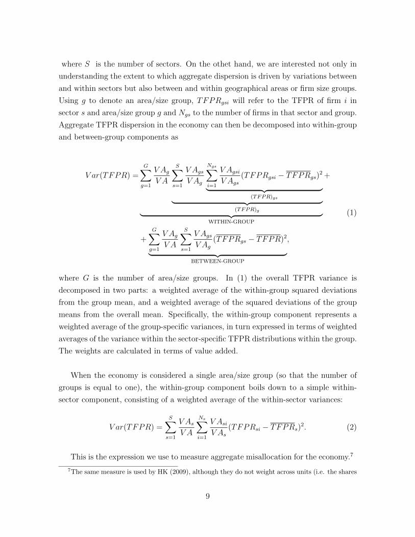
where S is the number of sectors. On the othet hand, we are interested not only in

understanding the extent to which aggregate dispersion is driven by variations between

and within sectors but also between and within geographical areas or firm size groups.

Using g to denote an area/size group, TFPRgsi will refer to the TFPR of firm i in

sector s and area/size group g and Ngs to the number of firms in that sector and group.

Aggregate TFPR dispersion in the economy can then be decomposed into within-group

and between-group components as

V ar(TFPR) =G∑

g=1

V Ag

V A

S∑s=1

V Ags

V Ag

Ngs∑i=1

V Agsi

V Ags

(TFPRgsi − TFPRgs)2

︸ ︷︷ ︸(TFPR)gs︸ ︷︷ ︸

(TFPR)g︸ ︷︷ ︸WITHIN-GROUP

+

+G∑

g=1

V Ag

V A

S∑s=1

V Ags

V Ag

(TFPRgs − TFPR)2

︸ ︷︷ ︸BETWEEN-GROUP

,

(1)

where G is the number of area/size groups. In (1) the overall TFPR variance is

decomposed in two parts: a weighted average of the within-group squared deviations

from the group mean, and a weighted average of the squared deviations of the group

means from the overall mean. Specifically, the within-group component represents a

weighted average of the group-specific variances, in turn expressed in terms of weighted

averages of the variance within the sector-specific TFPR distributions within the group.

The weights are calculated in terms of value added.

When the economy is considered a single area/size group (so that the number of

groups is equal to one), the within-group component boils down to a simple within-

sector component, consisting of a weighted average of the within-sector variances:

V ar(TFPR) =S∑

s=1

V As

V A

Ns∑i=1

V Asi

V As

(TFPRsi − TFPRs)2. (2)

This is the expression we use to measure aggregate misallocation for the economy.7

7The same measure is used by HK (2009), although they do not weight across units (i.e. the shares

9

3 Data description

We use two main databases. The first covers the universe of incorporated companies

(CERVED) with information from firms’ balance sheets that we use to compute ag-

gregate misallocation.8 This database accounts for 70% of manufacturing value added

from national accounts and the growth rate follows very closely the national one. Then,

in order to analyse the firm-level features of misallocation, we rely on a representative

sample of firms with more detailed information on firms’ characteristics that we use to

analyse firm-level misallocation (INVIND). We group manufacturing firms into 3-digit

sectors using the ATECO 2002 classification, which allows us to distinguish detailed

categories such as ‘machines for producing mechanic energy’, ‘machines for agriculture’,

‘tooling machines’, ‘machines for general use’, etc.9

In order to compute firm-level measures of TFPR as in HK, we need measures of

output as well as of labor and capital inputs. We measure the labor input using the cost

of labor and the capital stock using the book value of fixed capital net of depreciation,

while we take firms’ value added as a measure of the total revenue of the model as this

does not consider intermediate inputs. All variables are deflated through sector-specific

deflators (with base year 2007). We clean the database from outliers by dropping all

observations with negative values for real value added, cost of labor or capital stock.

We are left with a pooled sample of 1,740,000 firm-year observations for manufacturing

over the period 1993–2013. The average number of observations per firm is 12. To

compute firm-level TFPR we also need capital and labor shares at industry level. We

compute the labor share by taking the industry mean of labor expenditure on value

added measured at the firm level. We then set the capital share as one minus the

computed labor share.

V Asi/V As). Thus, compared to HK, our measure assigns more importance to misallocation in largerfirms.

8This database includes also micro enterprises with less than 10 employees.9The total number of 3-digit sectors is 91. We also use a more aggregate classification at 2-digit

and results hold. We exclude ‘coke and petroleum products’ and ‘other manufacturing n.e.c.’ frommanufacturing. These sectors have peculiar behaviors, whose study lies outside the scope of thispaper.

10

The second dataset is the main one we use for the analysis of firm-level misallocation

is the Bank of Italy’s annual “Survey of Industrial and Service Firms” (INVIND). We

focus on the open panel of representative Italian manufacturing firms with at least

50 employees. The survey contains detailed information on firm revenues, ownership,

production factors, year of creation and number of employees since 1984. Additional

information is drawn from “Centrale dei Bilanci” (CB), which contains balance sheet

data on around 30,000 Italian firms. INVIND data are matched with those from CB

using the tax identification number of each firm. We drop observations pre–1987, in

order to have a proper sample coverage, as well as those not matched with CB data.

We are left with a pooled sample of 19,924 firm-year observations over the 25-year

period 1987–2011, with an average of 11 observations per firm. We divide the INVIND

panel in low-tech and high-tech sectors using the OECD classification of manufacturing

industries according to their global technological intensity, based on R&D expenditures

respect to value added and production.10

Table 1 presents sectoral descriptive statistics from CERVED at 2-digits for average

real value added, capital stock and cost of labor over the period of observation, both in

absolute terms and in percentages with respect to the total.11 The sectors ‘machinery’,

‘metals’ and ‘textile and leather’ are the sectors with the largest numbers of firms and

represent 62% of the total number of manufacturing firms. Real value added ranges

from a mean of around 0.8m Euro in ‘wood’ to around 4.4m Euro in ‘vehicles’. Variation

in the average capital stock is sizable, ranging from around 1m Euro in ‘textile and

leather’ to around 4.9m Euro in ‘vehicles’. The cost of labor varies notably too, ranging

between 0.5m Euro in ‘wood’ and 3.2m Euro in ‘vehicles’.

In order to better understand the pattern of misallocation, we divide the dataset

10High-tech industries include firms that produce office, accounting and computing machines; ra-dio, TV and communication equipment; aircraft and spacecraft; medical, precision and optical instru-ments; electrical machinery and apparatus n.e.c.; motor vehicles, trailers and semi trailers; chemicalsexcluding pharmaceuticals; rail-road equipment and transport equipment n.e.c.; and machinery andequipment n.e.c. Low-tech industries account for firms that work in building and repairing of shipsand boats; rubber and plastic products; other non-metallic mineral products; basic metals and fab-ricated metal products; wood, pulp, paper; paper products; printing and publishing; food products;beverage and tobacco; textiles; and leather and footwear.

11We present the descriptive statistics for 2-digit sectors for ease of exposition, but the quantitativeanalysis is at 3-digit level.

11

into geographic and firm size cells. In particular, we group firms within each industry

into four main Italian macro-areas: Northwest, Northeast, Center, South and Islands.12

We also divide the firms in the dataset into four groups according to firm size: ‘micro’,

‘small’, ‘medium’ and ‘big’.13 We report the summary statistics of the main variables

divided by geographic area and size, both in absolute terms and percentages, in Table

2. Around two thirds of manufacturing firms are located in the Northern areas of the

country. In these areas, manufacturing firms’ value added, capital stock and cost of

labor are higher than the average. Looking at firm size, more than 88% of manufactur-

ing firms are ‘micro’ or ‘small’, while only 2.2% are ‘big’. However, ‘micro’ and ‘small’

firms account for only around 30% of total value added and input costs, whereas big

firms account for around 45%.

In Table 3 we present the summary statistics of firms clustered by sector-area and

by sector-size. For most of the industries the majority of firms are located in the

North. Moreover, practically all sectors are composed mainly by ‘micro’ and ‘small’

firms, with the majority of bigger manufacturing firms concentrated in ‘chemicals’,

‘food and tobacco’ and ‘vehicles industries’. Table 4 shows the relevance of firm size by

geographic area. In the Northwest more than half of the value added in manufacturing

comes from ‘big’ firms. Finally, Table 5 looks at the distribution of value added by

firm size across geographical areas. About 56% of value added produced by big firms

in the manufacturing sector comes from the Northwest, this confirms a strong overlap

between the Northwest region and big firms.

12We use the ISTAT (National institute of Statistics) classification of macro-areas. “Northwest”includes the regions Liguria, Lombardy, Piedmont and Aosta Valley; “Northeast” includes Emilia-Romagna, Friuli-Venezia Giulia, Trentino-South Tyrol and Veneto; “Center” includes Lazio, Marche,Tuscany and Umbria; “South and Islands” includes Abruzzi, Basilicata, Calabria, Campania, Molise,Apulia, Sicily and Sardinia.

13We use the European Commission classification of firms according to their turnover. “Mi-cro” are firms with a turnover < 2m Euros, “small” < 10m Euros, “medium” < 50m Euros,“big” > 50m Euros. See http://ec.europa.eu/growth/smes/business-friendly-environment/

sme-definition/index_en.htm.

12

We first investigate the misallocation pattern in the manufacturing sector by com-

puting the TFPR variance as described in Equation (2). The output of this exercise

(in logs) is depicted in Figure 4, where we also report the average TFPR based on the

same weighting scheme used for the variance. The figure shows that a large decline

in average TFPR occurred in the mid-nineties, followed by a temporary recovery from

2005 to 2007 and a new fall associated with the economic crisis with a drop of about

-10.5%. Moreover, aggregate misallocation (as measured by the variance of TFPR)

steadily and steeply increased between 1995 and 2009 and slightly decreased after its

peak in 2009. However, aggregate misallocation increased by almost 69% between 1995

and 2013 with most of the increase taking place in the first decade.14

To better understand the firm-level dynamics behind the aggregate patterns dis-

played in Figure 4, we compare the firm-level distributions of TFPR in 1995 with that

in 2013. This comparison, reported in Figure 5, shows quite clearly that the evolution

of TFPR highlighted above (i.e. decreasing average and increasing variance) mainly

occurred through a rising share of low productivity firms. When the comparison is

made, instead, between 2007 and 2013 (see Figure 6), the difference in the share of

low productivity firms is much less pronounced. In fact, recalling what we have seen

in Figure 4, 2007 represents a critical year for average TFPR but not for its variance

as this grows until 2009. Figure 7 shows the evolution of aggregate misallocation, cap-

tured by the variance of TFPR over the full sample of firms per-year. We can see that

misallocation raised sharply from 1995 to 2009, when it started a process of slow re-

version. This suggests that the aggregate decrease in TFPR occurred in the last years

compounds a long-run increase in misallocation with a crisis-related fall in average firm

productivity.

In principle, the increasing misallocation pattern documented in the aggregate

might hide substantial differences across sectors, areas and firm size categories. How-

ever, before going into the details of each dimension, we implement the decomposition

in Equation (1) in order to understand to what extent aggregate misallocation can be

14In order to have some insight about the trend of misallocation before 1993, we also use theINVIND database which starts in 1987–2011, but accounts for a more limited sample of firms above50 employees. This longer database confirms that the rise of misallocation is a phenomenon thatstarted in the mid-’90s and it was not a previously undergoing trend. In INVIND misallocation has asimilar trend with respect to CERVED, although the raise starts a couple of years later in 1997 andis quantitatively stronger.

13

4 The patterns of aggregate misallocation

traced back to differences in terms of TFPR dispersion across the categories. In Figure

8 we report the computed within and between components of aggregate TFPR vari-

ance for the three dimensions, along the whole period under consideration (1993–2013).

The message is clear-cut as the between component is always small compared with the

within component with only slight differences emerging across the three dimensions

(see Figures 9 and 10). Moreover, since the between components start growing only

after 2000, the increase in aggregate variance occurred between 1995 and 2000 is al-

most entirely driven by the within components. We wonder whether this pattern is

driven by firms’ entry and exit, so in Figure 11 we disentangle the pattern of within

misallocation for firms that are always in our data set (balanced panel) and for the full

sample that accounts also for entry and exit. Even if the level of misallocation is lower

for the balanced panel, the trend of misallocation is qualitatively very similar in both

samples. However, from a quantitative point of view, after 1995 misallocation increases

more significantly for the balanced panel than for the full sample; this implies that if

anything, the process of entry and exit is dampening the raise of misallocation, which

is consistent with the findings of Linarello and Petrella (2016).

As shown by Hsieh and Klenow (2009), TFPR can be expressed as a geometric

average of the marginal product of capital (MRPK) and labor (MRPL). Hence the

dispersion of TFPR and our measure of misallocation are going to be proportional to

MRPK and MRPL. Figure 12 looks at the patterns of MRPK and MRPL dispersion and

it shows that capital is the factor of production that experiences the sharpest increase

in its marginal product’s dispersion since the mid-1990s, although this pattern has

flattened out since the global financial crisis. To some extent the dispersion of MRPL

increased too, but it does not show a striking trend.15 This seems to suggest that the

capital market is a very important source of misallocation in Italy.

A first source of concern is that capital may be subject to adjustment costs (“time-

to-build”) that can lead to a higher dispersion simply due to a technology-driven ad-

justment process, which would be an efficient outcome. In order to explore whether

time to build can be a driver of our findings, we explore the stationarity of our firm-

15If we look at the change of the distribution of MRPK and MRPL between 1995 and 2013, wesee that MRPK experienced a fattening of both tails and it kept a very similar mean; whereas,the distribution of MRPL experienced a clear leftward shift with a significant decrease of the mean.Results are available upon request.

14

level misallocation measure ln(TFPRis/TFPRs

). The idea is that this ratio should

converge towards one over time if the adjustment process after a TFP shock is the main

driver of TFPR dispersion. Firstly, we consider the variance ratio statistics (Cochrane,

1988; Engel, 2000), defined as V ar(Xt+k −Xt)/V ar(Xt+1 −Xt), where X denotes the

relative log-TFPR averaged across sectors. For stationary series, the variance ratio

approaches a limit. The output of this exercise is reported in Figure 13. The pat-

tern suggests that the variation in firm-level misallocation tends to stabilise in a time

horizon of around fifteen years, which is a too long period for being consistent with

an adjustment cost story. We also run a series of unit root tests to investigate the

mean reversion property of this ratio. Table 6 reports the the Im-Pesaran-Shin (Im

et al., 2003) and the Fisher-type (Choi, 2001) tests for the presence of unit root. The

null hypothesis is rejected in all cases, entailing the series to be stationary and firms’

relative TFPR not being mean reverting.16

Another source of concern is related to measurement error in firms’ revenues and

inputs. As Bils et al. (2017) point out, this is likely to distort the misallocation anal-

ysis. In fact, a firm’s TFPR is higher when revenues are overstated and/or inputs are

understated: if, for example, the extent of revenue overstatement (input understate-

ment) systematically grows (shrinks) with firms’ true revenues (inputs), the dispersion

of measured TFPR is unequivocally biased upward. Bils et al. (2017) suggest to tackle

this issue by exploiting the intuition that, while without measurement error revenue

growth solely depends on TFPR and input growth, the presence of measurement error

introduces spurious correlation between firms’ TFPR and input growth. Their sug-

gested methodology allows us to evaluate the fraction of observed TFPR dispersion

reflecting the actual presence of distortions. In our estimation based on Bils et al.

(2017), this fraction amounts to 0.54, suggesting that more than fifty per cent of our

measured misallocation is not driven by measurement error and can thus be regarded

as true misallocation.17 More interesting for us, this fraction is relatively constant over

time (if anything slightly increasing) over our sample period, suggesting that, although

the level of misallocation has to be taken with caution, our discussion about the trend

in misallocation is mostly unaffected by measurement error issues.

16Analogous conclusions can be reached by carrying out the tests on the log-TFPR series.17 Bils et al. (2017) find that this ratio is 0.23 for the US,

15

5 Insights from regional and size patterns

To better understand the geographical distribution of the aggregate pattern, we

report the evolution of misallocation within macro-regions – i.e. the term V ar(TFPR)g

– in Figure 14.18 We note that i) TFPR in the South is on average always lower

than in the rest of Italy; ii) misallocation in the Northwest and the Center grew at

a considerably higher rate compared to the other areas; and iii) misallocation in the

South was higher than in the rest of Italy at the beginning of the period but, being quite

stable over time, ends up being lower than in the North at the end of the period.19.

The same analysis can be carried out in terms of firm size categories (see Figure 15)

and an important highlight is that misallocation grew in all groups but it affected more

heavily the bigger firms.

These results are puzzling because firms in the Northwest region and bigger firms

are traditionally more advanced and closer to the technological frontier. However,

this reveals important insights on the overall dynamics of misallocation. A possible

explanation for the raise of misallocation is that, for given level of frictions, the shocks

hitting firms have become more dispersed; this might be the result of a fast changing

technological frontier (due for instance to the IT revolution). To explore this possibility

we build on Griffith, Redding and Van Reenen (2004) and look at the average change

of R&D intensity between 1987-1993 and 1994-2007 in advanced countries as a proxy of

shocks to the technology frontier by sector. We measure R&D intensity as the share of

R&D expenditure over value added at the sectoral level. The countries we consider are

Canada, Denmark, Finland, France, Germany, Japan, Netherlands, Norway, Sweden,

United Kingdom, and United States. Results hold also if we take R&D intensity in

the United States only. Data are from the ANBERD database of the OECD.20 Figure

16 shows that there is a positive and significant correlation between the increase in

the R&D ratio in advanced countries and the increase in misallocation, such that an

increase in R&D intensity by one standard deviation is associated with an increase

18The underlying is assumption is that within sector misallocation should be less problematic withinmacro regions than at the national level, as moving factors should have lower adjustments costs. Thisexercise allows us to understand the geographical distribution of misallocation.

19For ease of exposition we do not show the graphs of group-specific distributions, but they supportthis finding.

20This is measured as the share of R&D expenditure over value added at the sectoral level. Dataare from the ANBERD database of the OECD.

16

in misallocation of 0.14 standard deviations (statistically significant at the 1% level).

Moreover, once we account for the sectoral composition of regions (or firm size), it

turns out that the implied “frontier shock” is higher in the Northwest (4.6%) and the

Center (5.1%) and lower in the Northeast (3.1%) and the South (2.2%). This follows

the ranking of the increase in misallocation by region highlighted above. The same

result applies if we look at the implied shock by firm size.

An implication of this result is that firms in the upper part of the productivity

distribution should be those that contribute more to the overall increase in misalloca-

tion. This is indeed the case, as shown by the contribution of each firm quartile to

the overall increase of misallocation in our sample.21 As we can see the top quartile

is the one that contributes the most the rise of aggregate misallocation. The produc-

tivity thresholds of firms entry and exit do not exhibit a particular trend, but they

are subject to standard year-to-year oscillation. On average, firms that enter a market

are 20% more productive than the average firm in that sector, whereas firms that exit

the market are 40% less productive than the average firm (Figure 17). This suggests

that movements of the cut-off for firms entry and exit are unlikely to drive the rise of

misallocation, which is actually the result of increased dispersion in the top quartile of

the distribution.

6 The impact of misallocation on aggregate TFP

The overarching message sent by the battery of figures and tables presented in the

previous section is that overall the stagnation of Italian productivity since the 1990’s

has been accompanied by a steady increase in misallocation. We now quantify the

impact that the increase in misallocation had on aggregate TFP during our period of

observation. In particular, we want to understand how much aggregate TFP in 2013

would have changed if misallocation had remained constant at the 1995 level.

21The standard deviation of log-TFPR is about 0.4 for firms in the top quartile and it is increasingover time. For firms in the 2nd and 3rd quartile it is slightly increasing after the crisis, but its level islow (0.1). Finally for firms in the bottom quartile, the dispersion if higher (0.6), but it is stable up tothe crisis and then decreases. The top and the bottom 1% of the distribution are trimmed from oursample

17

In the wake of HK, we proceed as follows. First, in each year t from 1995 to 2013

we evaluate the increase in aggregate output that could be achieved by completely

eliminating misallocation (i.e. by reallocating productive factors so as to equalize their

remunerations across all firms). In any given year, within the HK framework that

increase is dictated by the ratio between the observed aggregate output level Y and

the efficient aggregate output level Y ∗ in the absence of gaps in factor remunerations.

We can, therefore, evaluate the percentage increase in aggregate productivity that

could have been achieved in any year t by completely eliminating misallocation as:

% Gaint/within =

(YtY ∗t

)−1

− 1 (3)

Second, to understand how much aggregate TFP in year t would have changed if

misallocation had remained constant at the 1995 level, we can look at the percentage

relative change in the efficient-to-observed output ratios in the two years:

% Gaint/95 =

(Yt/Y

∗t

Y95/Y ∗95

)−1

− 1 (4)

When applied to our data, equation (4) implies that, if misallocation had remained

at its 1995 level, in 2013 aggregate TFP would have been 18% higher than its ac-

tual level. Moreover, the effect of misallocation on TFP peaked in the aftermath of

the global financial crisis leading to a 23% foregone productivity gain, but weak-

ened slightly after the Euro-debt crisis. So, even after netting out the spike in the

productivity penalty of misallocation associated with the crisis, the adverse effects of

misallocation on Italian productivity remain sizeable.22

From a size class and geographical perspective, the observed patterns are mainly

driven by misallocation across big firms and by firms in the Northwest. In fact, in the

22The quantitative results of this exercise are sensitive to the values chosen for the elasticity ofsubstitution σ between products sold by firms. In the baseline we set σ equal to 3 as in Hsieh andKlenow (2009). This is a conservative value also in light of Broda and Weinstein (2006) who find thatfor SITC-3 digits the average value of the elasticity of substitution after 1990 is about 4. Higher valueof the elasticity deliver stronger gains. The gain would be to 12% with σ equal to 2, and 19% with σequal to 4.

18

cases of big firms and the Northwest, TFP would have been 18% and 25% higher if

misallocation in 2013 had stayed at its 1995 level.

7 Productivity, misallocation, and firm character-

istics

In the previous section we have documented the important role played by rising

misallocation across Italian firms in the dismal evolution of Italian productivity since

the 1990’s. We have highlighted that the main source of misallocation comes from a

within industry component, especially in sectors where the world technological frontier

has expanded faster. Relative specialization in those sectors explains the patterns of

misallocation across geographical areas and firm size classes: accounting for the sectoral

composition of Italian regions and firm size classes implies that “frontier shocks” are

the strongest for Northern regions and big firms. This matches the relative increase in

misallocation across geographical areas and firm sizes.

To shed additional light on the relation between exposure to frontier shocks and mis-

allocation within industries, we now investigate which firm characteristics (“markers”)

are associated with firms being inefficiently sized. We look in particular at corporate

ownership and management, finance, workforce composition, internationalization and

innovation. In doing so, we rely on reduced form regressions at the firm level. The

econometric specifications that we implement allow us to identify correlations, but

not causation, of key firm characteristics with a firm’s TFPR relative to its sectoral

average. In particular, we run the following regression:

lnTFPRist

TFPRst

= β0 + β1Xist + δt + γs + εist, (5)

where i, s and t refer to firm, sector and year respectively; Xist is the marker (or vector

of markers) we want to analyze23; δt is a year dummy that captures common shocks to

all firms in a given year; γs is a sector fixed effects controlling for time-invariant sector

characteristics that can influence the effect of the marker on misallocation; εist is the

error term. This regression relates the log-ratio of a firm’s TFPR to the average TFPR

23For robustness, we also enter the markers with a squared term in order to allow for non-linearity.

19

of its sector with the chosen marker (or vector of markers). Thus, if our estimates

point to β1 > (<)0, we can conclude that firms with larger Xist are characterized by

higher (lower) relative TFPR.

In equation (5) the main variable of interest is marker Xist. Its coefficient β1 could

be zero in two different scenarios. First, it would be zero if the aggregate allocation of

resources were efficient, as TFPRis/TFPRs = 1 would hold for all firms. As we have

already seen, this is not the case in our data. Second, even if the allocation of resources

were not efficient, β1 would be zero if Xist did not directly affect relative TFPR. As in

the end only the second scenario is relevant, we can conclude that a non-zero estimate

for β1 reveals that the marker increases misallocation.24 In particular, larger (smaller)

values of the marker lead to more misallocation for positive (negative) estimated β1.

In other words, if the estimated β1 is positive, firms with relatively large Xist are

inefficiently small; vice versa, if the estimated β1 is negative, firms with relatively large

Xsit are inefficiently large.

Our benchmark specification is based on standard pooled OLS regression, always

including sector and year dummies.25 We have also run a number of different speci-

fications, including additional controls, lagged regressors, and firm effects. Moreover,

we have run these regressions by geographic area, firm size, and low- vs. high-tech

sectors.26 While the corresponding results are available upon request, for parsimony

we provide here a synthetic description of the most robust and policy relevant findings

based on the benchmark case with our aggregate sample.

For each marker, we run regression (5). Moreover, following HK, we infer the

firm-level output and capital distortions (“wedges”) and we use them as alternative

24In Calligaris et al. (2016) we show that a marker could still be linked to misallocation even if β1were zero, if it is related to the dispersion of the residuals of equation (5). We have checked whetherthis is the case and found no evidence, which implies that β1 6= 0 is the necessary and sufficientcondition for a marker to induce misallocation. We omit these results for parsimony but they areavailable from the authors on request.

25With respect to our aim of investigating the markers of misallocation, the most appropriatespecification does not include firm fixed effects. In fact, we are mainly interested in how cross-firmdifferences in relative TFPR are related to given firm characteristics. We are less concerned with theeffects of the within-firm variation in those characteristics across time.

26We use the OECD classification of manufacturing industries according to their global technologicalintensity, based on R&D expenditures with respect to value added.

20

dependent variables in (5).27 There is a higher capital distortion when the ratio of

labor compensation to the capital stock is high with respect to the one we would expect

from the industry output elasticities relative to capital and labor. In order to interpret

the regressions, it is important to keep in mind that capital and labor distortions are

each other’s mirror image, as a high labor distortion would show up as a low capital

distortion. This implies that a positive and significant coefficient of the capital wedge

on marker Xist, reveals that X is associated to higher capital distortion relative to

labor (without implying that labor distortion is zero) so that capital compensation

is too low relative to labor compensation, given the output elasticities of these two

factors. A negative and significant coefficient means instead that firms characterised

by marker X tend to suffer from high labor distortion relative to capital, so that labor

compensations are too low relative to capital. Similarly, the output wedge is large

when the labor share is small given the industry elasticity of output with respect to

labor.

Therefore, we run regression (5) using as dependent variable not only relative

TFPR, but also the output wedge and the capital wedge. The independent variables

(“markers”) we use refer to a series of usual suspects that include various proxies

for ownership, finance, labor force, innovation, foreign exposure, and cronysm. The

variables are listed in Table 7 and we discuss them in the corresponding subsections.28

7.1 Corporate ownership/control and governance

We construct an indicator of ownership type, distinguishing between firms con-

trolled by an individual or a family, a conglomerate, a financial institution, the public

sector or a foreign entity. As Michelacci and Schivardi (2013) already found that fam-

ily firms tend to choose activities with a lower risk/return profile compared to firms

27Hsieh and Klenow (2009) show that for firm i in sector s the capital and output distor-tions (‘wedges’) can be computed as τKis = αswLis/ [(1− αs) RKis] − 1 and τY is = 1 −σwLis / [(1− σ)(1− αs)PisYis].respectively, where w is the wage, R is the rental rate of capital,Pis is price of output and αs is the capital share of firm expenditures.

28In order to check if our results are driven by the financial crisis, we run all regressions also up to2008 only. Results are very similar qualitatively, quantitatively, and in terms of statistical significance.The only difference is for the regression on delocalisation, whose coefficient turns to be statisticallysignificant, but very similar in magnitude.

21

controlled by other entities, we expect family firms to have lower relative productivity

and thus to be inefficiently over-resourced with respect to other firms. This is exactly

what we find by regressing the relative TFPR on dummies for each ownership type,

using family controlled firms as the reference group (Table 8).

Specifically, we find that firms controlled by either a financial institution, a group,

or a foreign company have between 3% and 8% higher relative TFPR than family

controlled firms (column 1). Differently, we do not find any statistical difference of rel-

ative TFPR between public and family controlled firms. This implies that for instance

foreign controlled firms are too small and should be allocated more resources than

family owned firms. Column 2 of Table 8 confirms this finding by showing that these

types of firms suffer from higher output distortion with respect to family owned firms.

Moreover, column 3 highlights that these firms specifically suffer from an additional

distortion in terms of capital-labor ratio. In particular the negative coefficient implies

that they suffer more strongly of labor distortions and they should increase the labor

compensation with respect to capital, i.e. absorb a higher share of workers.

Reading these fundings through the lenses of the HK framework, they imply that

aggregate productivity would likely increase if family firms and government controlled

firms were acquired by private groups or foreign entities. On the other hand, keeping

corporate ownership unchanged, aggregate productivity would increase if misallocation

were reduced within all corporate ownership categories with the largest productivity

gains coming from firms controlled by groups and foreign entities.29

7.2 Finance

In the case of finance, we investigate the relevance of credit constraints, equity

emissions and relational banking. We also explore the impact of the introduction of

29Although the database is not representative in terms of young firms, we looked at the relationshipbetween age and relative TFPR. We did not find any significant relationship when only linear termsare considered. Things seem to change substantially when we allow for a squared term. In thatcase, our regression results suggest that the relation between relative TFPR and age are U-shaped.Unfortunately, the nature of our database prevents us from performing a robust analysis of otheraspects of governance.

22

the Euro on firms’ financial characteristics.

a. Credit constraint

We define credit constrained firms as those that declared that they would have

liked a higher level of debt (Table 9 ). We also use an alternative measure of credit

constraint based on the willingness of having more credit even at higher interest rates,

which delivers the same results.30 Both measures enter the regression with a lag in

order to mitigate endogeneity. In this way we capture how being credit constrained at

time t− 1 is correlated to TFPR and misallocation at time t.

In particular, we find that firms that are credit constrained at time t − 1 tend to

have lower relative TFPR at time t.31 This implies that credit constrained firms are

absorbing too many resources and should downsize, so in this sense the “right” firms

seem to be financially constrained. Moreover, Column 2 shows that credit constrained

firms are characterized by a negative and significant output distortion; this is equivalent

to saying that these firms are actually receiving an implicit subsidy, so it would be more

efficient if they exited the market. Finally, in credit-constrained firms the capital-labor

ratio is not significantly distorted.

b. Equity

We look at the relation of firms’ relative TFPR and distortions with the timing of

their equity emissions. In particular, we look at the correlation between relative TFPR

at time t and equity emissions at time t− 1, t, and t+ 1. In Table 10 we report results

for time t only, but there is virtually no difference with the other timings. We find

that firms that have lower relative TFPR in a given year tend to issue more equity

(either in the same year, the year after or the one before). This may suggest that

equity issuance may be a relevant source of funding when firms are hit by a negative

productivity shock, but at the same time it may also mean that equity buyers are not

allocating capital efficiently as these firms are too large given the productivity they

have and should absorb fewer resources.

30Results available upon request31This effect is particularly pervasive in low-tech industries.

23

An important issue about the effect of the Euro on productivity and misallocation

relates to the interest rate convergence that characterised peripheral countries thanks

to the common currency. The traditional argument, as in Gopinath et al. (2015)

and Benigno and Fornaro (2014), is that the availability of cheaper funds led to a

misallocation of capital towards low productive firms that rather than exiting the

market increased their leverage. We do not provide a formal test of this hypothesis,

but we look for observationally consistent facts. For instance, if this were the case,

we should observe a significant increase in leverage for firms with lower relative TFPR

after the introduction of the Euro.32

In Table 11 we can see that high leverage indeed characterizes lower TPFR firms.

This relation becomes significantly stronger after national exchange rate parities were

fixed to the Euro in 1999. This is consistent with the fact that the interest rate con-

vergence that followed the introduction of the Euro led to a misallocation of credit to

less productive firms that are disproportionately large given their productivity. Not

surprisingly, we also observe that more leveraged firms are characterised by a misallo-

cation of the capital-labor ratio as the share of capital is too large. However, this effect

did not increase significantly after the Euro.

d. Relational banking

We consider a firm as being involved in ‘relational banking’ if it declares that the

principal reason for dealing with its main bank is “personal relationship and assistance”.

In Table 12 we observe that relational banking is associate with lower relative TFPR,

so that the firms that engage in relational banking are larger than what they should

optimally be. This suggests that relational banking might be a key motivation for low

productive firms to choose a specific bank, perhaps because it grants more support

in time of need. Hence, relational banking may be a drag on aggregate productivity

because it diverts resources from more productive firms with weak banking connections

to less productive firms with strong banking connections.

32Leverage is defined as debt over total assets. By looking at this variable we check if firms’ debtincreased disproportionately with respect to total assets during the period of cheap credit that followedthe introduction of the Euro.

24

c. Euro effect

7.3 Workforce composition

The functioning of the labor market is one of the structural features of the Italian

economy that has been more extensively reformed since the 1990s.33 Misallocation is

less likely to emerge when less productive firms are free to reduce (and more productive

firms are free to increase) the amount of labor. In this perspective, by introducing more

flexibility in the labor market, the reforms that the Italian economy underwent in the

1990s should have induced a better allocation of labor. In this section we analyse

the relation between firms’ workforce and misallocation from different perspectives. In

particular we look at the Italian Wage Supplementation Scheme, which is the main

instrument of labor hoarding that firms use. We also look at the shares of temporary

and foreign workers that firms hire; and we analyse the role of skill intensity among

both blue- and white-collars.

a. Wage Supplementation Scheme (Cassa Integrazione Guadagni - CIG)

Firstly, we look at how intensively firms resorted to the Wage Supplementation

Scheme (“Cassa Integrazione Guadagni” - CIG) (variable “CIG share” - hours of CIG

over total hours worked). When firms are in distress, they can use this scheme to hoard

labor, so that workers suspend temporarily their job and receive a public benefit. The

key characteristic of this scheme is that it protects not only the worker, but also the

specific job match between worker and firm. This scheme can have either a positive or

negative effect on misallocation, because it facilitates labor hoarding guaranteeing to

firms and workers a useful buffer in downturns, but at the same time it might end up

protecting a job match that would be more efficient to break. Our methodology allows

us to understand in which direction productivity and misallocation are affected by this

specific policy tool.

33Two major reforms of the labor market took place: the Treu Law and the Biagi Law. Theformer was introduced in 1997 (law 196/97) with the aim of making the Italian labor market moreflexible. The main novelty of the Treu Law consisted in the introduction of temporary contracts andin the creation of Temporary Work Agencies (jobcenters were privatized and decentralized). TheTreu Package also modified the discipline of fixed-term contracts, modified the regulation related toemployment in the research sector and rose from 22 to 24 the age limit for apprenticeship contracts.The Biagi Law, introduced in 2003 (law 30/03), created new contractual forms and renovated someexisting ones, mainly affecting the subordinated workers.

25

Table 13 shows that the firms that use the CIG more intensively are largely over-

resourced and their size should be smaller than what it currently is. There is also a

positive and significant correlation with output distortion implying that these firms

are receiving an implicit subsidy, which is indeed the case. Finally, our results show

that, as it might be expected, firms using the CIG suffer from a larger labor distortion

relative to capital.

These findings support the idea that less productive firms are more likely to take

advantage of the CIG and that, through the associated (temporary) reduction in la-

bor costs, the CIG works against the reduction of the amount of labor used by low

productivity firms, thereby fostering misallocation especially on the labor side.34

b. Temporary workers

Table 14 and 15 analyze the association of temporary and foreign workers with

our measures of misallocation. We construct the two variables “term empl share” and

“foreign empl share”. The former is expressed in terms of the ratio of the number of

temporary employees to the total number of employees at the end of the year. The

latter is, instead, measured as the ratio of the average number of foreign workers to the

average number of workers in a given year. Our sample begins from 1999 for temporary

workers and from 2003 for foreign workers.

We find that firms that use a higher share of temporary workers have higher relative

TFPR, so they are inefficiently under-resourced and their size should be larger than

what it actually is.35 At the same time, these firms suffer from a significantly stronger

distortion on capital inputs relative to labor (while we do not find a significant associ-

ation with output distortions). A possible explanation could be that more productive

34To go more into the details of these relationships, we build the variable “YearSwitch CI”, takingvalue one in the year in which the firm starts resorting to CIG, and run contemporaneous and one-yearlagged fixed effects regressions, finding that the decision to start using CIG is associated with lowerrelative TFPR.

35These findings support the idea that higher TFPR firms are more likely to take the opportunity ofresorting to temporary work. This result is in sharp contrast with Daveri and Parisi (2015), who finda negative correlation between a firm’s share of workers in a temporary contract and its productivity.However, the different productivity measure and the different time period (2001–2003 in their case)may explain the difference.

26

firms find stronger distortions in the capital market and, given the complementarity

between capital and labor, they tend to respond favoring a higher share of temporary

and more flexible workers.

As for foreign workers, we do not find that this marker is significantly associated

with misallocation. The coefficient on relative productivity in Table 15 is not statis-

tically different from zero. However, we find some positive and significant correlation

with the capital distortion, which signals that firms relying more on foreign workers

tend to suffer from stronger capital distortions relative to labor. Nevertheless, this

does not result into broader misallocation.

c. Skill intensity

We look at two measures of skill-intensity: the share of white collars holding a

degree (Table 16) and the share of blue collars holding a degree (Table 17). We are

able to observe these two variables only in 2010 and 2011, thereby we run a cross-section

regression for the two years together.36

Firms with a higher share of high skilled workers among white collars have higher

TFPR on average, hence they should be allocated more inputs to increase their size.37

These firms suffer also from a large output distortion and from a relatively larger

distortion for labor relative to capital, where the labor distortion could be related to

both skilled and unskilled labor. However, if we look at the share of skilled workers

among blue collars, we do not find any significant association with misallocation or

output distortion, but only a marginally significant association with stronger distortions

in labor input relative to capital.

7.4 Internationalization

We focus on two main dimensions of firms’ internationalisation, delocalisation and

foreign direct investment. In Table 18 we look at the correlation between misallocation

36We also run the regressions for the two years separately and the results are similar.37This result is particularly strong for big firms and for low-tech firms.

27

and wether firms delocalized part of their production process, whereas in Table 19 we

look at the correlation between FDI and misallocation. In both cases we do not find

evidence of resource misallocation for firms engaging with these types of international

activities with respect to those that do not. This does not imply, however, that within

those groups there is nomisallocation, but given the low number of observations, we

do not have enough power to analyse this aspect.

Another stylized fact about productivity and internationalisation is the well-known

higher productivity of the exporting firms, as compared to non-exporters. Given the

nature of our sample, in which more than 80% of the firms export, we have to some-

how take this evidence for granted. We have nonetheless considered the intensity of

the export activity, measured in terms of the export share of revenues, finding some

evidence of a positive relationship with relative TFPR.38

7.5 Innovation

Innovation is a fairly reasonable marker of both productivity and misallocation.

The relationship can in principle go both ways. On the one hand, innovation can be

thought to foster productivity; on the other hand, more productive firms (e.g. Melitz,

2003) and/or firms with higher revenues (e.g. Bustos, 2011) can display a higher

propensity to innovate. If the innovation choice is made in a dynamic context with

adjustment costs for capital, a positive relationship with misallocation can be expected

(Asker, Collard-Wexler and De Loecker, 2014). To investigate the role of innovation,

we consider the share of intangible assets (associated, essentially, with R&D, marketing

and branding) on firms’ total assets.

Table 20 shows that a higher share of intangible assets is associated with higher

relative TFPR.39 This implies that firms that invest more in innovation tend to be

under-resourced and should have larger size. Moreover, these firms tend to suffer from

a larger distortion in the allocation of capital relative to labor. This is consistent with

38The variability in the data does not allow for a proper analysis of this issue. Given the lowvariability in the data, the relationship emerges only when controls are introduced for the exportshare in t− 1 and t+ 1, or the nonlinearity in the relationship is taken into account.

39We also enter the regressor with a lag and the results are very similar.

28

the view that credit provision to firms that innovate may play a key role in reducing

misallocation.

While our database does not allow us to address innovation using alternative and

more focused measures, this evidence is in line with recent studies on the productivity

effects of intangible assets, such as Battisti, Belloc and Del Gatto (2015), who find

that these assets are positively associated with both TFP and technology adoption,

and suggest a key role of firms’ innovation choices as markers of misallocation.

7.6 Combining markers: a short horse-race

We complete our investigation of the firm markers associated with relative produc-

tivity and misallocation by running the regressions on different subsets of indepen-

dent variables entered simultaneously. This should give some guidance on the relative

importance of these variables. More specifically, we look at the share of graduates

among white collars, innovation, family ownership, reliance on the wage supplementa-

tion scheme (CIG), and the share of temporary employment. We focus on variables

that are available over subsequent years and are consistently part of our panel and not

just of some year-specific cross-section. There might be some concern of collinearity be-

tween the variables we consider. Hence, Table 21 looks at the cross-correlations among

these variables showing that correlations are never above 0.27 (in absolute value), which

reveals a low degree of collinearity.

Table 22 summarises the main results. As some of the variables are dummies

(i.e. “family ownership”), whereas the others are continuous variables, comparing

the magnitude of the coefficients is difficult. Hence, we focus more on their relative

statistical significance. The results show that the share of graduates among white

collars and the use of the wage supplementation scheme (CIG) are the statistically most

significant markers of misallocation, although of opposite sign (firms with a high share

of graduates are too small and those using the CIG are too large). Family ownership

and, to some extent, innovation are also two significant markers with opposite signs.

However, the share of temporary workers loses significance with respect to the results

presented in Table 14. In terms of output distortion, the most significant markers are

29

again the share of graduates among white collars, which has a positive and significant

coefficient (implying an implicit tax), and the use of CIG, which has a negative and

significant coefficient (implying an implicit subsidy). Finally, in terms of the capital-

labor ratio, innovative and family-owned firms are the ones with the strongest distortion

in terms of capital, whereas firms with a higher share of white-collar graduates confirm

to suffer from a significant distortion in terms of labor.

These findings, in particular the strong significance of the share of graduates among

white collars and the CIG, can be interpreted as two sides of the same coin. The share of

high-skill employees among white collars drives firm technological and organizational

innovation, which in turn increases firm productivity relative to competitors. In an

efficient process of creative destruction labor should seamlessly flow from firms with

falling relative productivity to firms with rising relative productivity thereby enhancing

aggregate productivity. This process of efficient reallocation is impaired if firms with

falling relative productivity can use the wage supplementation scheme to keep them

afloat when faced not only with contingent problems (as in the original spirit of the

CIG) but also with structural problems (as in the consolidated practice of the CIG).

More generally, our findings on the importance of the different markers suggest

that firms more likely to keep up with the technological frontier are inefficiently small

and thus under-resourced. These are the firms that employ a larger share of graduates

and invest more in intangible assets. On the contrary, firms less likely to keep up are

inefficiently large and thus over-resourced. These are the firms that have a large share

of workers under a wage supplementation scheme, that are family managed, and that

are financially constrained. We interpret this pattern as evidence that rising within-

industry misallocation is consistent with an increase in the volatility of idiosyncratic

shocks to firms due to their heterogeneous ability to respond to sectoral “frontier

shocks” in the presence of sluggish reallocation of resources.

8 Conclusions and policy implications

We have provided a detailed analysis of the patterns of misallocation in Italy since

the early 1990s. In particular, we have shown that the extent of misallocation has

30

substantially increased since 1995, and that this increase can account for a large fraction

of the Italian productivity slowdown since then. We have shown that the increase in

misallocation has mainly risen within than between sectors, increasing more witihin

those in which the world technological frontier has expanded faster.

We have highlighted that rising misallocation has hit firm categories that tradition-

ally are the spearhead of the Italian economy, in particular firms in the Northwest and

big firms. We have argued that relative specialization in sectors where the world tech-

nological frontier has expanded faster helps explaining the patterns of misallocation

across geographical areas and firm size classes. The broader lesson is that part of the

explanation of the recent productivity puzzle in other advanced economies may lie in a

generalised growing difficulty of reallocating resources between firms in sectors where

technology has been changing faster rather than between sectors with different speeds

of technological change.

We have shed additional light on the relation between exposure to “frontier shocks”

and misallocation within industries by investigating which firm characteristics are as-

sociated with firms being inefficiently sized. We found evidence that inefficiently small

under-resourced firms are those that, by employing a larger share of graduates and

investing more in intangible assets, are more likely to be keeping up with the tech-

nological frontier. Vice versa, inefficiently over-resourced firms are those that, being

featuring larger shares of workers under wage supplementation, more family managers

and stricter financial constraints, are more likely to be falling behind the technological

frontier. We have interpreted this pattern as evidence consistent with rising within-

industry misallocation being associated with increasing volatility of idiosyncratic shocks

to firms due to their heterogeneous ability to respond to sectoral “frontier shocks” in

the presence of sluggish reallocation of resources.

Our findings provide the ground for a policy-oriented discussion, to which we now

turn.

The main policy implications we highlight are the following:

• “Within-misallocation” matters more than “between-misallocation”:

This implies that, in order to raise productivity, rather than trying to switch

31

resources between sectors, geographical areas and firm size classes, policy inter-

vention should aim at allocating capital and labor to the best performing firms

within these categories. Policy intervention should therefore focus less on moving

capital and labor from, e.g., textile to electronics, than on facilitating the mobil-

ity of workers and capital towards the most productive firms within the textile

sector. Similarly, higher benefits would be reaped by moving the factors of pro-

duction to the most productive firms within depressed geographical areas rather

than moving them to more vibrant areas. This represents both an opportunity

and a challenge. An opportunity, because moving factors within sector or area is

less costly than across them; but also a challenge, because it is harder to deter-

mine what prevents high-productivity firms from expanding and low-productivity

firms from shrinking within the same sector or geographical area. More generally,

setting the framework conditions for the proper functioning of market-driven re-

allocations could be more effective than pursuing traditional industrial policies

aimed at ‘picking the winning sectors/regions’.

• There are a “North issue” as well as a “Large firm issue”: The rise of mis-

allocation and the subsequent decline of productivity in the traditional ‘engines’

of the Italian economy should be a source of major concern. The regional di-

mension indicates that misallocation has increased particularly in the Northwest,

traditionally the core of the Italian productive system. And the size dimension

suggests that the increase has been particularly strong among large firms. The

two events are not unrelated, as the Northwest is where larger firms tend to be

headquartered. These trends indicate that a lot of attention should be devoted

to policies targeted at improving the efficiency of the allocative process within

the category of large firms, such as labor market regulation, antitrust rules and

the system of public subsidies.

• A larger share of firms survives despite low productivity levels: The

increase in misallocation is to a large extent due to the increase in the share of

firms that are inefficiently over-resourced. This fact points to the inefficiency of

the institutions and regulations that govern the process of firm restructuring. We

see as particularly relevant: a) the regulation of firm bankruptcy procedures and

the efficiency of the judicial system in reallocating the assets of distressed firms

- these aspects have been subject to various reforms in the recent past, whose

32

results should hopefully become apparent over the next years. Developments

in this area should be closely monitored; b) the process of credit allocation by

banks that might lead to “zombie lending”, whereby credit is extended to low

productivity firms to keep them from going bankrupt; c) the diffusion of financial

operators specialized in firm restructuring and turnaround, such a private equity

firms - the market of private equity funds is still underdeveloped in Italy, possibly

due to their regulation and to the constraints on firm restructuring.

• The system of unemployment benefits needs to be reformed with more

focus on the “worker” than on the “job”: Our results show that the Italian

wage supplementation scheme (“Cassa Integrazione Guadagni”) is disproportion-

ately used by low productivity firms and is associated with higher misallocation.

The problem with this type of scheme is that it protects the job match between

workers and firms even if it is no longer productive. This hinders the process

of creative destruction that would lead to workers’ reallocation towards more

productive firms. This is especially the case whenever the scheme, rather than

being used as a temporary safeguard as in its original spirit, is used on a more

prolonged basis. In this respect, a universal unemployment benefit where unem-

ployed workers receive a subsidy, without preserving the job, could lead to less

misallocation of workers and higher productivity. This is the direction in which

recent reforms included in the Italian “Jobs Act” seem to be going.

• Investments in intangible assets are important: Our results show that

firms with a higher investment share in intangible fixed assets (such as R&D,

branding, and marketing) are more likely to be inefficiently under-resourced.

Public support to firms engaging this type of investments can provide impor-

tant incentives towards such productivity-enhancing activities; the recent Italian

public program called “Industry 4.0” goes in that direction. Another example of

reforms that could help along this dimension is the development of a non-banking

component of the financial markets. In fact, venture capital and private equity

could promote the access to credit by highly innovative, risky firms that would

be otherwise credit constrained.

• Graduates play a crucial role among white collars: Our results show that

firms with a higher number of graduates among their white-collars are inefficiently

under-resourced. Italy has a lower share of graduates than other European coun-

33

tries. Pro-active policies that encourage more tertiary education are warranted.

Skill mismatches might be more likely among highly educated workers, because

firms find it hard to fill positions requiring a high level of specific skills with the

appropriate candidates. This calls into question both the “production” of human

capital through the school system and its “deployment” to firms through formal

placement networks.

Beyond Italian specificities, several of these implications may apply more broadly

to other advanced economies facing their own “productivity puzzles”.

34

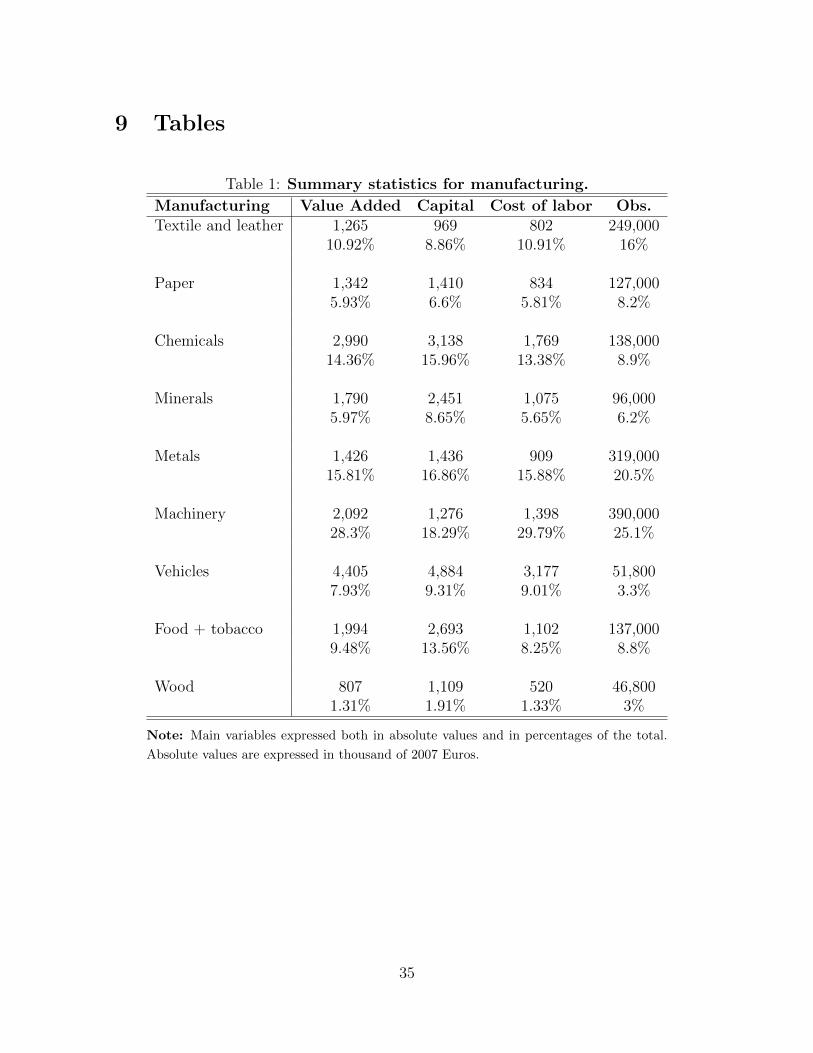
9 Tables

Table 1: Summary statistics for manufacturing.

Manufacturing Value Added Capital Cost of labor Obs.Textile and leather 1,265 969 802 249,000

10.92% 8.86% 10.91% 16%

Paper 1,342 1,410 834 127,0005.93% 6.6% 5.81% 8.2%

Chemicals 2,990 3,138 1,769 138,00014.36% 15.96% 13.38% 8.9%

Minerals 1,790 2,451 1,075 96,0005.97% 8.65% 5.65% 6.2%

Metals 1,426 1,436 909 319,00015.81% 16.86% 15.88% 20.5%

Machinery 2,092 1,276 1,398 390,00028.3% 18.29% 29.79% 25.1%

Vehicles 4,405 4,884 3,177 51,8007.93% 9.31% 9.01% 3.3%

Food + tobacco 1,994 2,693 1,102 137,0009.48% 13.56% 8.25% 8.8%

Wood 807 1,109 520 46,8001.31% 1.91% 1.33% 3%

Note: Main variables expressed both in absolute values and in percentages of the total.

Absolute values are expressed in thousand of 2007 Euros.

35

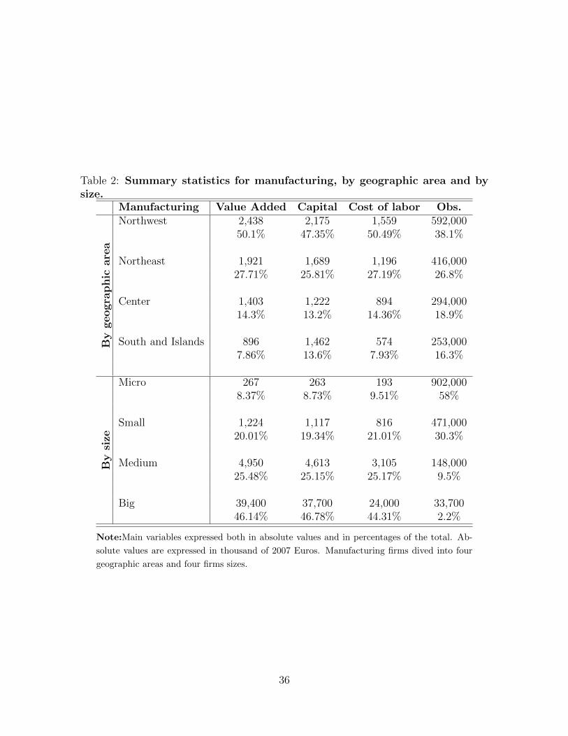
Table 2: Summary statistics for manufacturing, by geographic area and bysize.

Manufacturing Value Added Capital Cost of labor Obs.

By

geogra

ph

icare

a

Northwest 2,438 2,175 1,559 592,00050.1% 47.35% 50.49% 38.1%

Northeast 1,921 1,689 1,196 416,00027.71% 25.81% 27.19% 26.8%

Center 1,403 1,222 894 294,00014.3% 13.2% 14.36% 18.9%

South and Islands 896 1,462 574 253,0007.86% 13.6% 7.93% 16.3%

By

size

Micro 267 263 193 902,0008.37% 8.73% 9.51% 58%

Small 1,224 1,117 816 471,00020.01% 19.34% 21.01% 30.3%

Medium 4,950 4,613 3,105 148,00025.48% 25.15% 25.17% 9.5%

Big 39,400 37,700 24,000 33,70046.14% 46.78% 44.31% 2.2%

Note:Main variables expressed both in absolute values and in percentages of the total. Ab-

solute values are expressed in thousand of 2007 Euros. Manufacturing firms dived into four

geographic areas and four firms sizes.

36

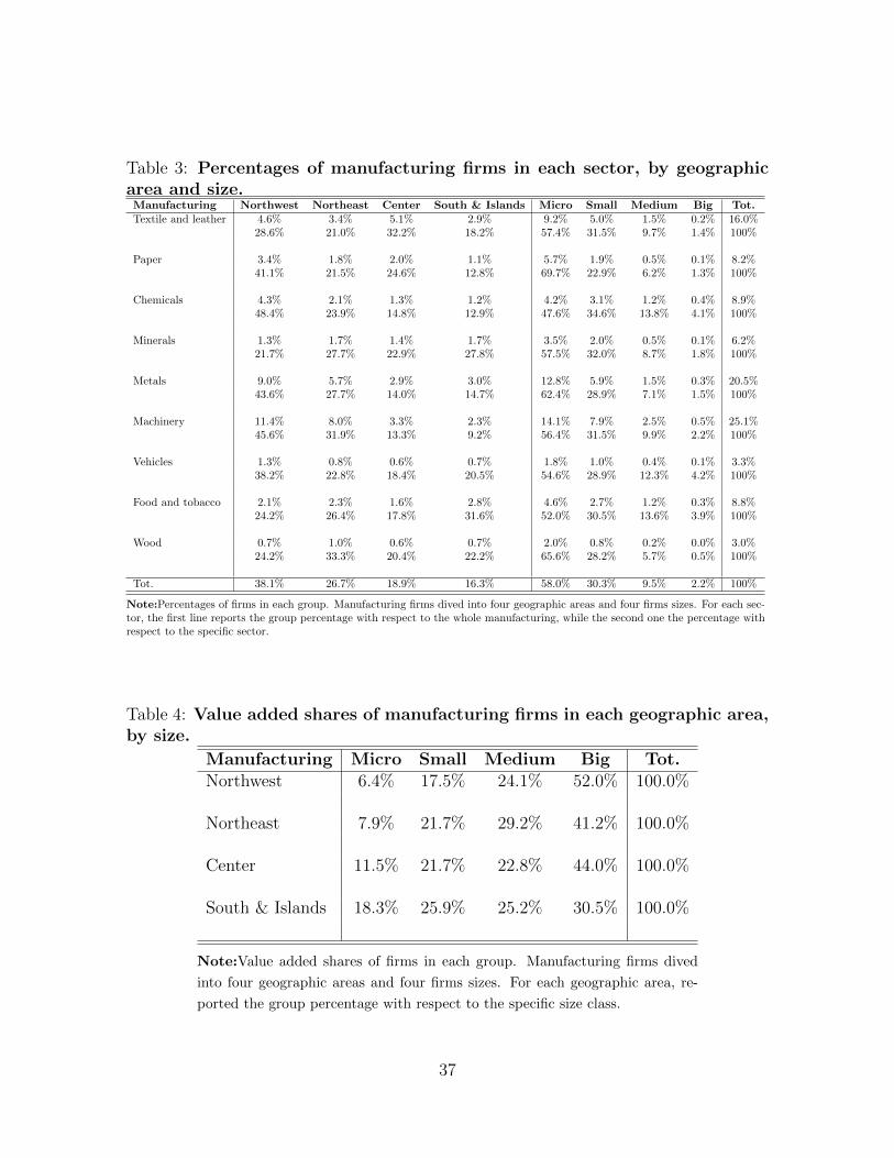
Table 3: Percentages of manufacturing firms in each sector, by geographicarea and size.Manufacturing Northwest Northeast Center South & Islands Micro Small Medium Big Tot.Textile and leather 4.6% 3.4% 5.1% 2.9% 9.2% 5.0% 1.5% 0.2% 16.0%

28.6% 21.0% 32.2% 18.2% 57.4% 31.5% 9.7% 1.4% 100%

Paper 3.4% 1.8% 2.0% 1.1% 5.7% 1.9% 0.5% 0.1% 8.2%41.1% 21.5% 24.6% 12.8% 69.7% 22.9% 6.2% 1.3% 100%

Chemicals 4.3% 2.1% 1.3% 1.2% 4.2% 3.1% 1.2% 0.4% 8.9%48.4% 23.9% 14.8% 12.9% 47.6% 34.6% 13.8% 4.1% 100%

Minerals 1.3% 1.7% 1.4% 1.7% 3.5% 2.0% 0.5% 0.1% 6.2%21.7% 27.7% 22.9% 27.8% 57.5% 32.0% 8.7% 1.8% 100%

Metals 9.0% 5.7% 2.9% 3.0% 12.8% 5.9% 1.5% 0.3% 20.5%43.6% 27.7% 14.0% 14.7% 62.4% 28.9% 7.1% 1.5% 100%

Machinery 11.4% 8.0% 3.3% 2.3% 14.1% 7.9% 2.5% 0.5% 25.1%45.6% 31.9% 13.3% 9.2% 56.4% 31.5% 9.9% 2.2% 100%

Vehicles 1.3% 0.8% 0.6% 0.7% 1.8% 1.0% 0.4% 0.1% 3.3%38.2% 22.8% 18.4% 20.5% 54.6% 28.9% 12.3% 4.2% 100%

Food and tobacco 2.1% 2.3% 1.6% 2.8% 4.6% 2.7% 1.2% 0.3% 8.8%24.2% 26.4% 17.8% 31.6% 52.0% 30.5% 13.6% 3.9% 100%

Wood 0.7% 1.0% 0.6% 0.7% 2.0% 0.8% 0.2% 0.0% 3.0%24.2% 33.3% 20.4% 22.2% 65.6% 28.2% 5.7% 0.5% 100%

Tot. 38.1% 26.7% 18.9% 16.3% 58.0% 30.3% 9.5% 2.2% 100%

Note:Percentages of firms in each group. Manufacturing firms dived into four geographic areas and four firms sizes. For each sec-tor, the first line reports the group percentage with respect to the whole manufacturing, while the second one the percentage withrespect to the specific sector.

Table 4: Value added shares of manufacturing firms in each geographic area,by size.

Manufacturing Micro Small Medium Big Tot.Northwest 6.4% 17.5% 24.1% 52.0% 100.0%

Northeast 7.9% 21.7% 29.2% 41.2% 100.0%

Center 11.5% 21.7% 22.8% 44.0% 100.0%

South & Islands 18.3% 25.9% 25.2% 30.5% 100.0%

Note:Value added shares of firms in each group. Manufacturing firms dived

into four geographic areas and four firms sizes. For each geographic area, re-

ported the group percentage with respect to the specific size class.

37

Table 5: Value added shares of manufacturing firms in size class, by geo-graphic area.

Manufacturing Northwest Northeast Center South & Islands Tot.Micro 37.6% 26.0% 19.4% 17.0% 100.0%

Small 43.6% 30.5% 15.6% 10.3% 100.0%

Medium 47.2% 32.1% 12.8% 7.8% 100.0%

Big 56.1% 25.0% 13.7% 5.2% 100.0%

Note:Value added shares of firms in each group. Manufacturing firms dived into four geographic areas

and four firms sizes. For each size class, reported the group percentage with respect to each geographic

area.

38

Table 6: Unit root tests on relative TFPR

Test Statistic p-value

Im-Pesaran-Shin Statistic p-valueW-t-bar (a) -17.2958 0.0000W-t-bar (b) * -63.9714 0.0000

Fisher-type, Augmented DickeyFuller (c)Inverse chi-squared(degrees of fr. 3476) 5901.691 0.0000Inverse normal -8.8742 0.0000Inverse logit t(degrees of fr. 8669) -13.9079 0.0000Modified inv. chi-squared 29.0925 0.0000

Fisher-type, Augmented DickeyFuller (c) *Inverse chi-squared(degrees of fr. 3476) 6539.15 0.0000Inverse normal -12.8297 0.0000Inverse logit t(degrees of fr. 8599) -19.645 0.0000Modified inv. chi-squared 36.7378 0.0000

Fisher-type, PhillipsPerron (d)Inverse chi-squared(degrees of fr. 3476) 7465.222 0.0000Inverse normal -21.5148 0.0000Inverse logit t(degrees of fr. 8639) -29.4953 0.0000Modified inv. chi-squared 47.8446 0.0000

Fisher-type, PhillipsPerron (d) *Inverse chi-squared(degrees of fr. 3476) 8073.704 0.0000Inverse normal -26.0377 0.0000Inverse logit t(degrees of fr. 8614) -35.8587 0.0000Modified inv. chi-squared 55.1425 0.0000

*Trend included

Serially correlated errors:(a) 1.03 lags - chosen by AIC;(b) 1.72 lags - chosen by AIC;(c) 1 lag Augmented Dickey-Fuller;(d) 1 lag Newey-West.

39

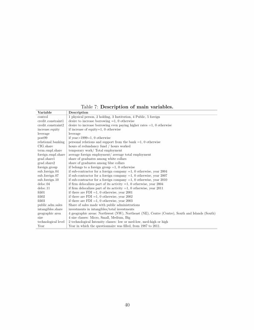
Table 7: Description of main variables.Variable Descriptioncontrol 1 physical person, 2 holding, 3 Institution, 4 Public, 5 foreigncredit constraint1 desire to increase borrowing =1, 0 otherwisecredit constraint2 desire to increase borrowing even paying higher rates =1, 0 otherwiseincrease equity if increase of equity=1, 0 otherwiseleverage leveragepost99 if year>1999=1, 0 otherwiserelational banking personal relations and support from the bank =1, 0 otherwiseCIG share hours of redundancy fund / hours workedterm empl share temporary work/ Total employmentforeign empl share average foreign employment/ average total employmentgrad share1 share of graduates among white collarsgrad share2 share of graduates among blue collarsforeign group if belongs to a foreign group =1, 0 otherwisesub foreign 04 if sub-contractor for a foreign company =1, 0 otherwise, year 2004sub foreign 07 if sub-contractor for a foreign company =1, 0 otherwise, year 2007sub foreign 10 if sub-contractor for a foreign company =1, 0 otherwise, year 2010deloc 04 if firm delocalizes part of its activity =1, 0 otherwise, year 2004deloc 11 if firm delocalizes part of its activity =1, 0 otherwise, year 2011fdi01 if there are FDI =1, 0 otherwise, year 2001fdi02 if there are FDI =1, 0 otherwise, year 2002fdi03 if there are FDI =1, 0 otherwise, year 2003public adm sales Share of sales made with public administrationsintangibles share investments in intangibles/total investmentsgeographic area 4 geographic areas: Northwest (NW), Northeast (NE), Centre (Centre), South and Islands (South)size 4 size classes: Micro, Small, Medium, Bigtechnological level 2 technological Intensity classes: low or med-low, med-high or highYear Year in which the questionnaire was filled, from 1987 to 2011.

40

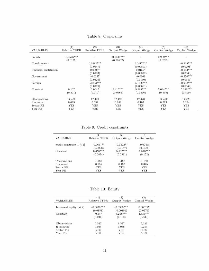
Table 8: Ownership

(1) (2) (3) (4) (5) (6)VARIABLES Relative TFPR Relative TFPR Output Wedge Output Wedge Capital Wedge Capital Wedge

Family -0.0526*** - -0.0346*** - 0.209*** -(0.0125) (0.00532) (0.0262)

Conglomerate 0.0582*** 0.0417*** -0.219***(0.0147) (0.00593) (0.0291)

Financial Institution 0.0308* 0.0159* -0.133***(0.0183) (0.00812) (0.0368)

Government -0.0237 -0.0169 -0.250***(0.0326) (0.0160) (0.0547)

Foreign 0.0803*** 0.0498*** -0.238***(0.0176) (0.00681) (0.0369)

Constant 0.107 0.0647 5.415*** 5.388*** 5.094*** 5.299***(0.221) (0.219) (0.0464) (0.0456) (0.465) (0.469)

Observations 17,420 17,420 17,420 17,420 17,420 17,420R-squared 0.029 0.032 0.098 0.102 0.293 0.294Sector FE YES YES YES YES YES YESYear FE YES YES YES YES YES YES

Table 9: Credit constraints

(1) (2) (3)VARIABLES Relative TFPR Output Wedge Capital Wedge

credit constraint 1 [t-1] -0.0657** -0.0322** -0.00445(0.0298) (0.0157) (0.0485)

Constant 0.658*** 5.537*** 6.516***(0.0824) (0.0381) (0.152)

Observations 1,188 1,188 1,188R-squared 0.155 0.132 0.375Sector FE YES YES YESYear FE YES YES YES

Table 10: Equity

(1) (2) (3)VARIABLES Relative TFPR Output Wedge Capital Wedge

Increased equity (at t) -0.0629*** -0.0305*** 0.000297(0.0151) (0.00801) (0.0276)

Constant -0.147 5.258*** 4.635***(0.240) (0.163) (0.439)

Observations 9,527 9,527 9,527R-squared 0.035 0.076 0.255Sector FE YES YES YESYear FE YES YES YES

41

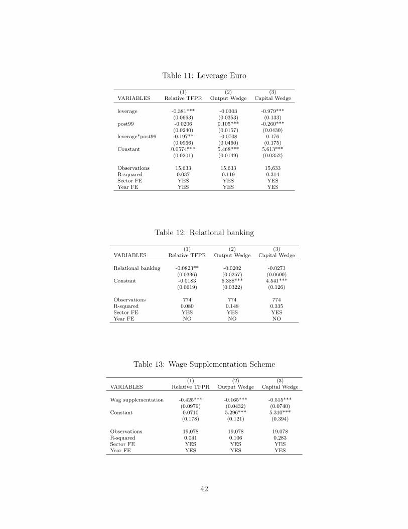
Table 11: Leverage Euro

(1) (2) (3)VARIABLES Relative TFPR Output Wedge Capital Wedge

leverage -0.381*** -0.0303 -0.979***(0.0663) (0.0353) (0.133)

post99 -0.0206 0.105*** -0.260***(0.0240) (0.0157) (0.0430)

leverage*post99 -0.197** -0.0708 0.176(0.0966) (0.0460) (0.175)

Constant 0.0574*** 5.468*** 5.613***(0.0201) (0.0149) (0.0352)

Observations 15,633 15,633 15,633R-squared 0.037 0.119 0.314Sector FE YES YES YESYear FE YES YES YES

Table 12: Relational banking

(1) (2) (3)VARIABLES Relative TFPR Output Wedge Capital Wedge

Relational banking -0.0823** -0.0202 -0.0273(0.0336) (0.0257) (0.0600)

Constant -0.0183 5.388*** 4.541***(0.0619) (0.0322) (0.126)

Observations 774 774 774R-squared 0.080 0.148 0.335Sector FE YES YES YESYear FE NO NO NO

Table 13: Wage Supplementation Scheme

(1) (2) (3)VARIABLES Relative TFPR Output Wedge Capital Wedge

Wag supplementation -0.425*** -0.165*** -0.515***(0.0979) (0.0432) (0.0740)

Constant 0.0710 5.296*** 5.310***(0.178) (0.121) (0.394)

Observations 19,078 19,078 19,078R-squared 0.041 0.106 0.283Sector FE YES YES YESYear FE YES YES YES

42

Table 14: Temporary employment, share of total workforce

(1) (2) (3)VARIABLES Relative TFPR Output Wedge Capital Wedge

Temporary employment share 0.116** -0.0398 0.597***(0.0565) (0.0280) (0.120)

Constant -0.0687 5.384*** 4.832***(0.173) (0.111) (0.375)

Observations 11,825 11,825 11,825R-squared 0.028 0.072 0.246Sector FE YES YES YESYear FE YES YES YES

Table 15: Foreign employment, share of total workforce

(1) (2) (3)VARIABLES Relative TFPR Output Wedge Capital Wedge

Foreign empoloyment share 0.127 -0.00505 0.705*(0.140) (0.0513) (0.366)

Constant -0.116 5.352*** 4.997***(0.219) (0.173) (0.469)

Observations 6,331 6,331 6,331R-squared 0.037 0.073 0.238Sector FE YES YES YESYear FE YES YES YES

Table 16: Share of graduates, white collars

(1) (2) (3)VARIABLES Relative TFPR Output Wedge Capital Wedge

Graduate share, white collars 0.359*** 0.105*** -0.241*(0.0765) (0.0308) (0.133)

Constant -0.308 5.514*** 5.039***(0.332) (0.0286) (0.630)

Observations 1,412 1,412 1,412R-squared 0.080 0.152 0.279Sector FE YES YES YESCross section Year 2000 and 2010 2000 and 2010 2000 and 2010

43

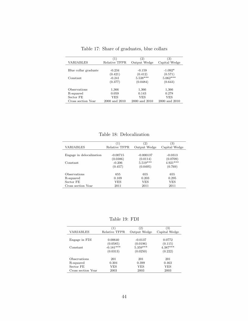
Table 17: Share of graduates, blue collars

(1) (2) (3)VARIABLES Relative TFPR Output Wedge Capital Wedge

Blue collar graduate -0.234 -0.159 -1.092*(0.421) (0.412) (0.571)

Constant -0.241 5.538*** 5.062***(0.377) (0.0484) (0.643)

Observations 1,366 1,366 1,366R-squared 0.059 0.143 0.278Sector FE YES YES YESCross section Year 2000 and 2010 2000 and 2010 2000 and 2010

Table 18: Delocalization

(1) (2) (3)VARIABLES Relative TFPR Output Wedge Capital Wedge

Engage in delocalization -0.00715 -0.000137 -0.0313(0.0386) (0.0114) (0.0709)

Constant -0.206 5.519*** 4.921***(0.457) (0.0495) (0.769)

Observations 655 655 655R-squared 0.109 0.203 0.295Sector FE YES YES YESCross section Year 2011 2011 2011

Table 19: FDI

(1) (2) (3)VARIABLES Relative TFPR Output Wedge Capital Wedge

Engage in FDI 0.00640 -0.0137 0.0772(0.0585) (0.0196) (0.115)

Constant -0.181*** 5.359*** 4.387***(0.0313) (0.0250) (0.222)

Observations 201 201 201R-squared 0.304 0.399 0.463Sector FE YES YES YESCross section Year 2003 2003 2003

44

Table 20: Innovation

(1) (2) (3)VARIABLES Relative TFPR Output Wedge Capital Wedge

Intangible assets, share 0.144*** -0.00188 0.377***(0.0381) (0.0160) (0.0688)

Constant -0.0796 5.377*** 4.849***(0.176) (0.110) (0.398)

Observations 11,689 11,689 11,689R-squared 0.030 0.071 0.247Sector FE YES YES YESYear FE YES YES YES

45

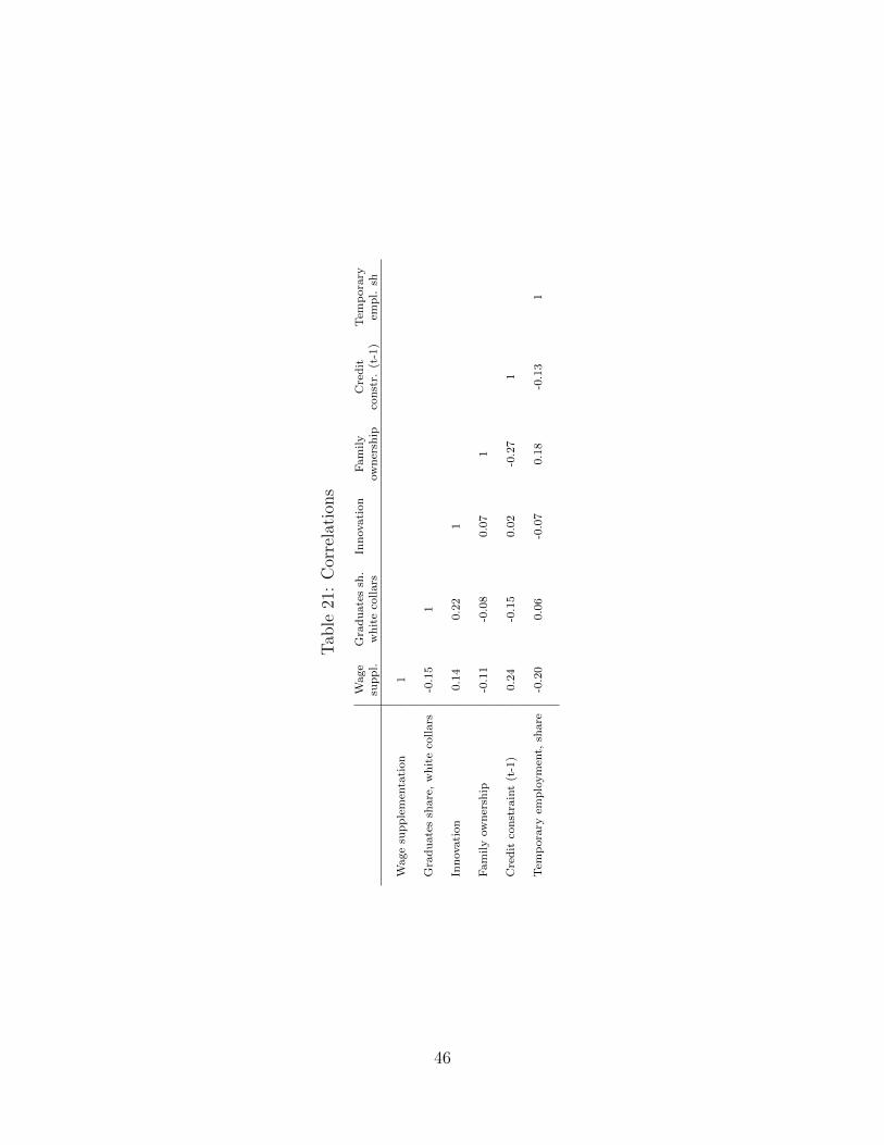
Tab

le21

:C

orre

lati

ons

Wage

Gra

du

ate

ssh

.In

novati

on

Fam

ily

Cre

dit

Tem

pora

rysu

pp

l.w

hit

eco

llars

ow

ner

ship

con

str.

(t-1

)em

pl.

sh

Wage

sup

ple

men

tati

on

1

Gra

du

ate

ssh

are

,w

hit

eco

llars

-0.1

51

Inn

ovati

on

0.1

40.2

21

Fam

ily

ow

ner

ship

-0.1

1-0

.08

0.0

71

Cre

dit

con

stra

int

(t-1

)0.2

4-0

.15

0.0

2-0

.27

1

Tem

pora

ryem

plo

ym

ent,

share

-0.2

00.0

6-0

.07

0.1

8-0

.13

1

46

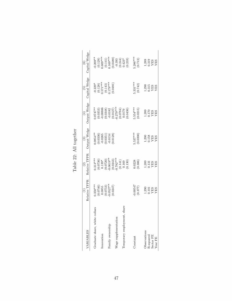
Tab

le22

:A

llto

geth

er

(1)

(2)

(3)

(4)

(5)

(6)

VA

RIA

BL

ES

Rel

ati

ve

TF

PR

Rel

ati

ve

TF

PR

Ou

tpu

tW

edge

Ou

tpu

tW

edge

Cap

ital

Wed

ge

Cap

ital

Wed

ge

Gra

du

ate

share

,w

hit

eco

llars

0.3

50***

0.3

13***

0.0

854**

0.0

747**

-0.2

29*

-0.2

69**

(0.0

746)

(0.0

736)

(0.0

336)

(0.0

353)

(0.1

28)

(0.1

29)

Inn

ovati

on

0.0

855

0.1

39*

-0.0

265

-0.0

0886

0.5

71***

0.6

09***

(0.0

753)

(0.0

720)

(0.0

351)

(0.0

348)

(0.1

43)

(0.1

41)

Fam

ily

ow

ner

ship

-0.0

527**

-0.0

619**

-0.0

154

-0.0

182

0.1

79***

0.1

69***

(0.0

247)

(0.0

243)

(0.0

128)

(0.0

127)

(0.0

491)

(0.0

488)

Wage

sup

ple

men

tati

on

-0.7

82***

-0.2

79***

-0.3

93

(0.1

41)

(0.0

784)

(0.2

44)

Tem

pora

ryem

plo

ym

ent,

share

0.1

69

0.0

179

0.4

23*

(0.1

30)

(0.0

436)

(0.2

33)

Con

stant

-0.0

0547

0.0

228

5.5

37***

5.5

54***

5.3

31***

5.2

86***

(0.3

77)

(0.3

06)

(0.0

390)

(0.0

215)

(0.7

42)

(0.7

12)

Ob

serv

ati

on

s1,2

90

1,2

89

1,2

90

1,2

89

1,2

90

1,2

89

R-s

qu

are

d0.1

01

0.1

31

0.1

58

0.1

70

0.3

15

0.3

19

Sec

tor

FE

YE

SY

ES

YE

SY

ES

YE

SY

ES

Yea

rF

EY

ES

YE

SY

ES

YE

SY

ES

YE

S

47

10 Figures

Figure 1: TFP pattern since the global financial crisis (2007=100)

90

92

94

96

98

100

102

2007 2008 2009 2010 2011 2012 2013 2014 2015

Eurozone12 UnitedKingdom UnitedStates

Data: Conference Board

Figure 2: Contribution to value added growth, Italy

Data: EU-Klems

48

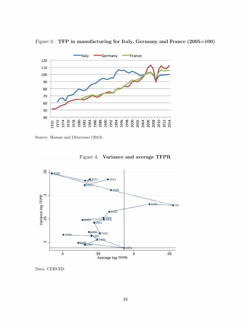
Figure 3: TFP in manufacturing for Italy, Germany and France (2005=100)

Source: Hassan and Ottaviano (2013)

Figure 4: Variance and average TFPR

1993 1994

1995

19961997

1998

1999 2000

2001200220032004

2005

2006 2007

2008

2009

20102011

2012

2013

.2.2

5.3

.35

Var

ianc

e lo

g-T

FP

R

.5 .55 .6 .65Average log-TFPR

Data: CERVED

49

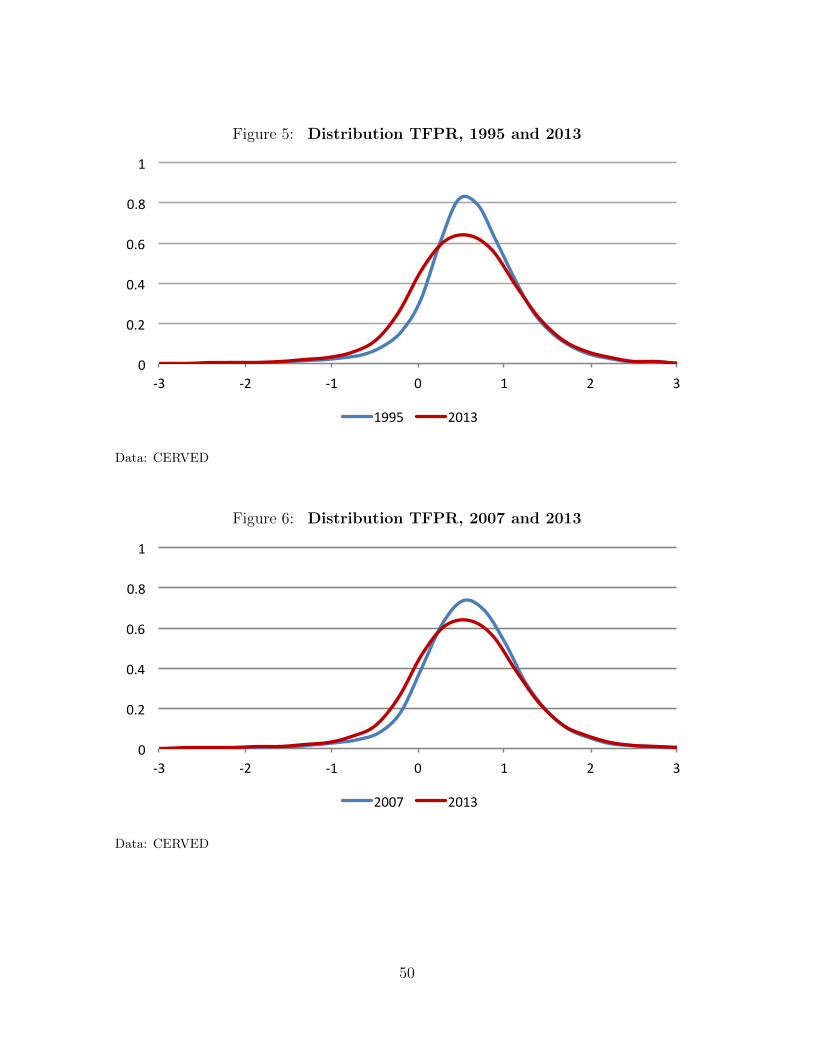
Figure 5: Distribution TFPR, 1995 and 2013

0

0.2

0.4

0.6

0.8

1

-3 -2 -1 0 1 2 3

1995 2013

Data: CERVED

Figure 6: Distribution TFPR, 2007 and 2013

0

0.2

0.4

0.6

0.8

1

-3 -2 -1 0 1 2 3

2007 2013

Data: CERVED

50

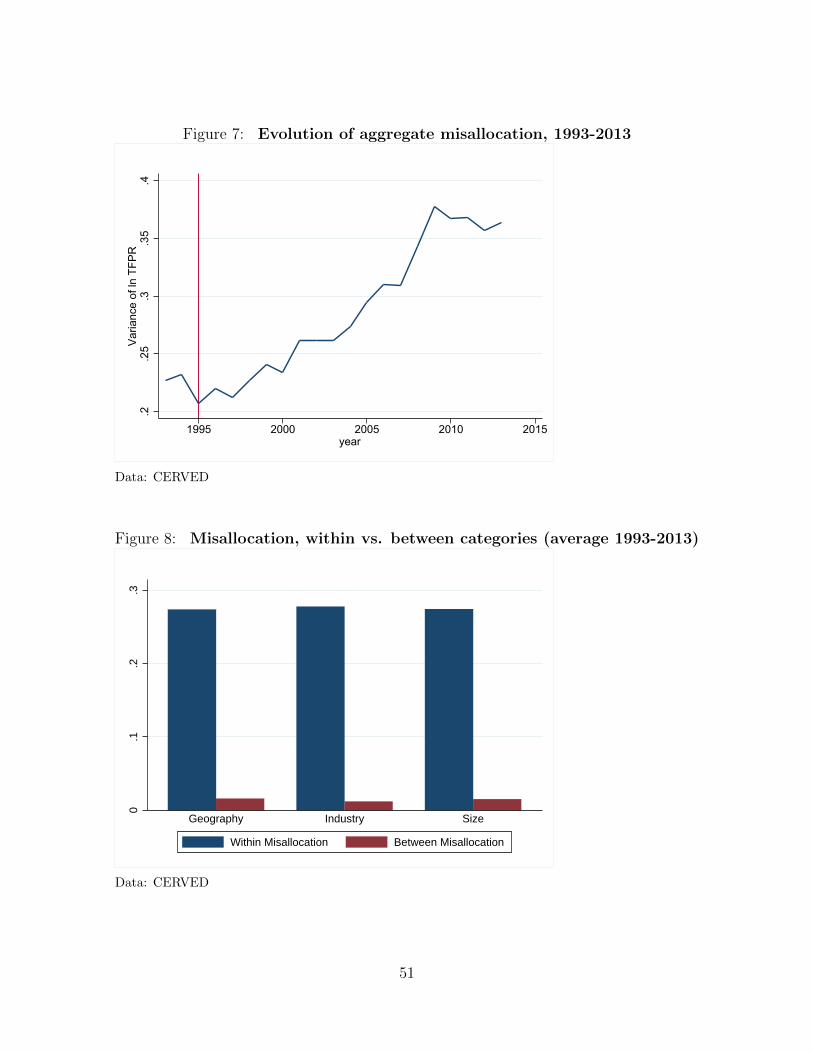
Figure 7: Evolution of aggregate misallocation, 1993-2013.2

.25

.3.3

5.4

Var

ianc

e of

ln T

FPR

1995 2000 2005 2010 2015year

Data: CERVED

Figure 8: Misallocation, within vs. between categories (average 1993-2013)

0.1

.2.3

Geography Industry Size

Within Misallocation Between Misallocation

Data: CERVED

51

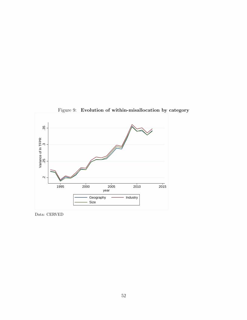
Figure 9: Evolution of within-misallocation by category

.2.2

5.3

.35

Var

ianc

e of

ln T

FP

R

1995 2000 2005 2010 2015year

Geography IndustrySize

Data: CERVED

52

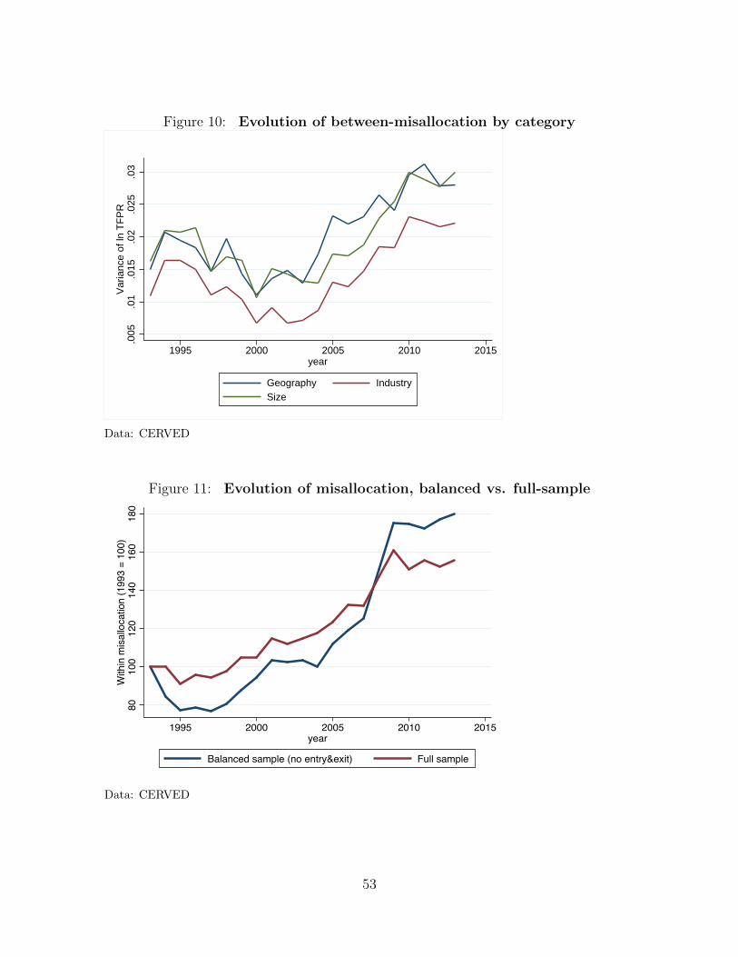
Figure 10: Evolution of between-misallocation by category.0

05.0

1.0

15.0

2.0

25.0

3V

aria

nce

of ln

TF

PR

1995 2000 2005 2010 2015year

Geography IndustrySize

Data: CERVED

Figure 11: Evolution of misallocation, balanced vs. full-sample

8010

012

014

016

018

0W

ithin

misa

lloca

tion

(199

3 =

100)

1995 2000 2005 2010 2015year

Balanced sample (no entry&exit) Full sample

Data: CERVED

53

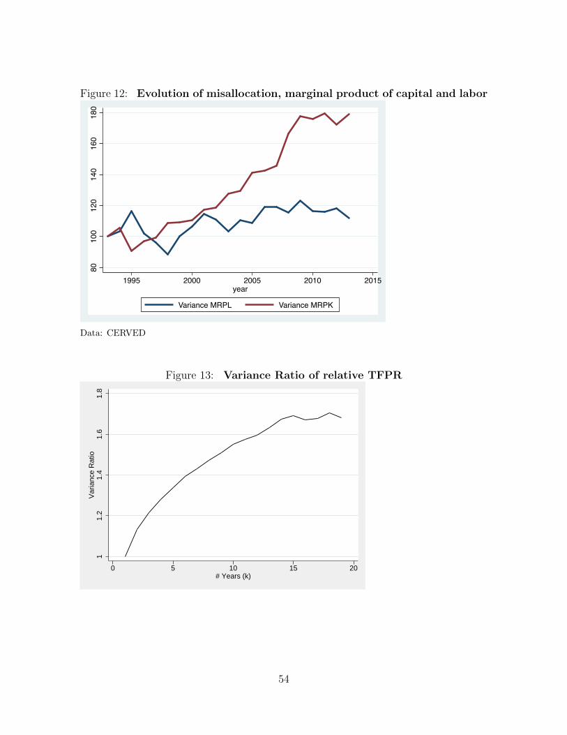
Figure 12: Evolution of misallocation, marginal product of capital and labor80

100

120

140

160

180

1995 2000 2005 2010 2015year

Variance MRPL Variance MRPK

Data: CERVED

Figure 13: Variance Ratio of relative TFPR

11.

21.

41.

61.

8V

aria

nce

Rat

io

0 5 10 15 20# Years (k)

54

Figure 14: Evolution of misallocation by geographic area.1

5.2

.25

.3.3

5.4

Var

ianc

e of

ln T

FP

R

1995 2000 2005 2010 2015year

Northwest NortheastCenter South

Data: CERVED

Figure 15: Evolution of misallocation by firm size

.15

.2.2

5.3

.35

Var

ianc

e of

ln T

FP

R

1995 2000 2005 2010 2015year

Small MediumBig

Data: CERVED

55

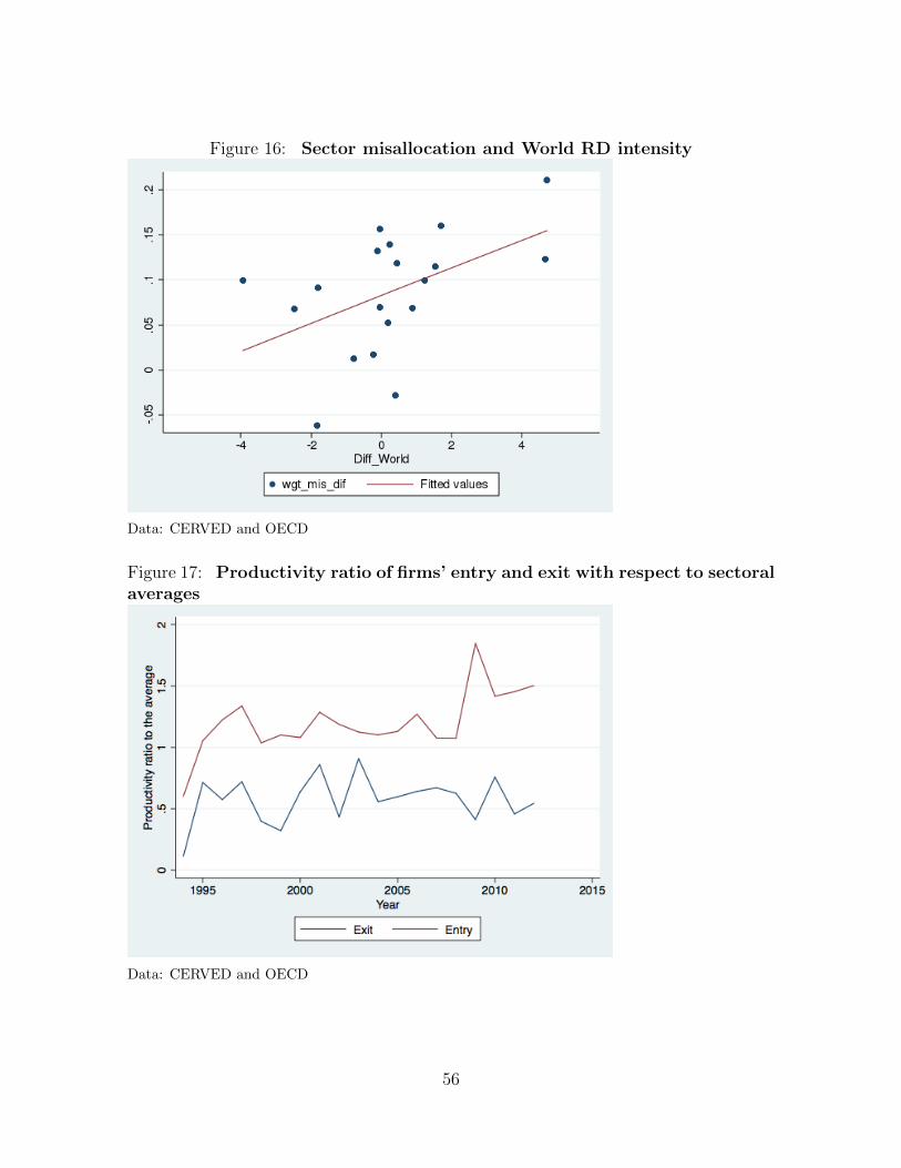
Figure 16: Sector misallocation and World RD intensity

Data: CERVED and OECD

Figure 17: Productivity ratio of firms’ entry and exit with respect to sectoralaverages

Data: CERVED and OECD

56

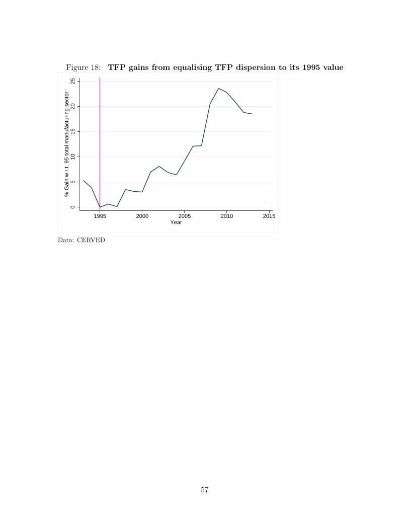
Figure 18: TFP gains from equalising TFP dispersion to its 1995 value0

510

1520

25%

Gai

n w

.r.t.

95

tota

l man

ufac

turin

g se

ctor

1995 2000 2005 2010 2015Year

Data: CERVED

57

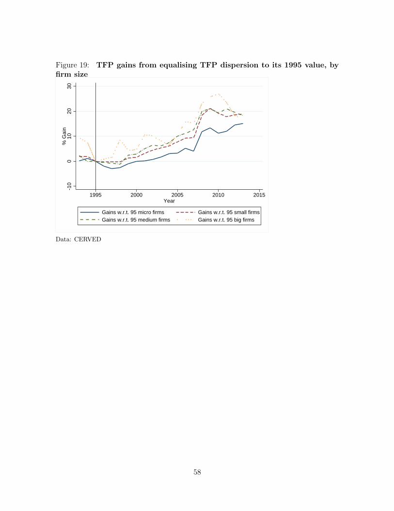
Figure 19: TFP gains from equalising TFP dispersion to its 1995 value, byfirm size

-10

010

2030

% G

ain

1995 2000 2005 2010 2015Year

Gains w.r.t. 95 micro firms Gains w.r.t. 95 small firmsGains w.r.t. 95 medium firms Gains w.r.t. 95 big firms

Data: CERVED

58

Figure 20: TFP gains from equalising TFP dispersion to its 1995 value, bygeographic area

-10

010

2030

% G

ain

1995 2000 2005 2010 2015Year

Gains w.r.t. 95 Northwest Gains w.r.t. 95 NortheastGains w.r.t. 95 Center Gains w.r.t. 95 South & Island

Data: CERVED

References

[1] Altomonte, C., Aquilante, T. (2012). The EU-EFIGE/Bruegel-

unicredit dataset (No. 753). http://bruegel.org/2012/10/

the-eu-efigebruegel-unicredit-dataset/

[2] Asker, J., Collard-Wexler, A., De Loecker, J. (2014), Dynamic Inputs and Re-

source (Mis)Allocation, Journal of Political Economy, 122(5): 1013-1063.

[3] Bandiera, O., Prat, A., and R. Sadun, (2015), Managing the Family Firm: Evi-

dence from CEOs at Work, CEPR Discussion Paper 10379.

[4] Barba-Navaretti, G., Bugamelli, M., Schivardi, F., Altomonte, C., Horgos, D.,

Maggioni, D. (2010), The global operations of European firms, Second EFIGE

Policy Report.

[5] Bellone, F., Mallen-Pisano, J. (2013): Is misallocation higher in France than in

the United States?, GREDEG Working Paper, N. 38.

59

[6] Bils, M., Klenow, P., and C. Ruane ( 2017), Misallocation or Mismeasurement?,

Stanford University, mimeo.

[7] Bloom, N., Sadun, R., Van Reenen, J. (2012). Americans Do IT Better: US

Multinationals and the Productivity Miracle, The American Economic Review ,

102(1): 167-201.

[8] Bollard, A., Klenow, P., Sharma, G. (2013), India’s Mysterious Manufacturing

Miracle , Review of Economic Dynamics, 16(1): 59-85.

[9] Broda, C., Weinstein, D.E. (2006), Globalization and the gains from variety, Quar-

terly Journal of Economics, 121(2): 541-585.

[10] Bugamelli, M., Schivardi, F., Zizza, R. (2010), The euro and firm restructuring, in

Europe and the euro, A. Alesina and F. Giavazzi (editors), University of Chicago

Press.

[11] Bugamelli, M., Cannari, L., Lotti, F., Magri, S. (2012), The innovation gap of

Italy’s production system: roots and possible solutions, Bank of Italy Occasional

Paper, n.121.

[12] Calligaris, S. (2015), Misallocation and Total Factor Productivity in Italy: Evi-

dence from Firm?Level Data, Labour, 29(4): 367-393.

[13] Calligaris, S., Del Gatto, M., Hassan, F., Ottaviano, G.I.P., Schivardi, F. (2016).

”Italy’s Productivty Conundrum”, European Commission Discussion Paper n.

030.

[14] Cette, G., Fernald, J.G.., and B. Mojon. (2016). The pre-Great Recession slow-

down in productivity, European Economic Review,vol. 88, issue C, 3-20

[15] Chen, K., Irarrazabal A. (2014): The role of allocative efficiency in a decade of

recovery, Review of Economic Dynamics, 18: 523-550

[16] Choi, I., (2001), Unit root tests for panel data, Journal of International Money

and Finance, vol. 20, issue 2, 249-272

[17] Cochrane, J.H., (1988). How big is the random walk in GNP?, Journal of Political

Economy, vol. 96, 893920.

60

[18] Crespo, A., Segura-Cayela, R. (2014), Understanding competitiveness, EUI Work-

ing Papers, 2.

[19] Daveri, F., Parisi, M. L. (2015) Experience, Innovation, and Productivity Empir-

ical Evidence from Italy’s SlowdownILR Review, 68 (4): 889-915.

[20] De Loecker, J., and P. Goldberg (2014). Firm performance in a global market,

Annual Review of Economics 6, 201-227.

[21] De Nardis, S. (2014), Efficienza e specializzazione, Nomisma 9 October 2014.

[22] Dias, D., Marques, C. R., Richmond, C. (2014), Misallocation and productivity

in the lead up to the Eurozone crisis, Banco de Portugal Working Paper, No.

w201411.

[23] Engel, C., (2000). Long-run PPP may not hold after all, Journal of International

Economics, vol. 51, issue 2, 243-273.

[24] Faini, R., Sapir, A. (2005) Un modello obsoleto? Crescita e specializzazione

dell’economia italiana, Oltre il declino, Bologna: il Mulino, 19-77.

[25] Fernald, J.G. (2014) Productivity and Potential Output Before, During, and After

the Great Recession, Federal Reserve Bank of San Francisco, Working Paper 2014-

15.

[26] Foster, L., Haltiwanger, J. and Syverson C. (2008) Reallocation, firm turnover,

and efficiency: Selection on productivity or profitability?. The American Economic

Review 98(1), 394-425.

[27] Foster, L., Grim, C., Haltiwanger, J. and Wolf, Z. (2017) Macro and Micro Dy-

namics of Productivity: From Devilish Details to Insights. CES Working Paper

17-41R

[28] Garcoa-Santana, M., Moral-Benito, E., Pijoan-Mas, J., Ramos, R. (2016), Grow-

ing like Spain: 1995-2000, Banco de Espana Working Paper No. 1609.

[29] Gopinath, G., Kalemli-Ozcan, S., Karabarbounis, L., Villegas-Sanchez, C. (2017),

Capital Allocation and Productivity in South Europe, Quarterly Journal of Eco-

nomics, forthcoming.

61

Griffith, R., Redding, S., and J. Van Reenen. (2004) Mapping the Two Faces of

RD: Productivity Growth in a Panel of OECD Industries, Review of Economics

and Statistics, vol. 86, issue 4, 883-895.

[30] Haltiwanger, D. (2016), Firm Dynamics and Productivity: TFPQ, TFPR, and

Demand-Side Factors, Economıa 17, 3-26.

[31] Hassan, F., Ottaviano, G.I.P. (2013). Productivity in Italy: the Great Unlearning,

VoxEu, 14 December 2013

[32] Head, K. and Mayer, T. (2014), Gravity Equations: Workhorse, Toolkit, and

Cookbook. In Helpman, E., Rogoff, K., and Gopinath, G., editors, Handbook of

International Economics, volume 4, pages 131-195. Elsevier.

[33] Hsieh, C., Klenow, P. (2009), Misallocation and manufacturing TFP in China and

India, Quarterly Journal of Economics, 124(4): 1403-1448.

[34] Im, K.S., Pesaran, M., and Y. Shon, (2003), Testing for unit roots in heterogeneous

panels, Journal of Econometrics, vol. 115, issue 1, 53-74

[35] Linarello, A., Petrella, A. (2016), Productivity and Reallocation: evidence from

the universe of Italian firms, Bank of Italy, Occasional Paper, n.353.

[36] Lippi, F., Schivardi, F. (2014), Corporate Control and Executive Selection, Quan-

titative Economics, 5(2), 417-456.

[37] Lusinyan, L. and Muir, D. (2013). Assessing the Macroeconomic Impact of Struc-

tural Reforms: The Case of taly. IMF, Working Paper No. 13/22.

[38] Michelacci, C., Schivardi, F. (2013), Does Idiosyncratic Business Risk Matter for

Growth?, Journal of the European Economic Association, 11(2): 343-368.

[39] Pellegrino, B., Zingales, L. (2014) Diagnosing the Italian disease, Unpublished

manuscript.

[40] Ziebarth, N. (2013), Are China and India Backwards? Evidence from the 19th

Century U.S. Census of Manufactures , Review of Economic Dynamics, 16(1):

86-99.

62

CENTRE FOR ECONOMIC PERFORMANCE Recent Discussion Papers

1519 Alex Bell Raj Chetty Xavier Jaravel Neviana Petkova John Van Reenen

Who Becomes an Inventor in America? The Importance of Exposure to Innovation

1518 Randolph Bruno Nauro Campos Saul Estrin Meng Tian

Economic Integration, Foreign Investment and International Trade: The Effects of Membership of the European Union

1517 Fabrice Defever José-Daniel Reyes Alejandro Riaño Miguel Eduardo Sánchez-Martín

Special Economic Zones and WTO Compliance: Evidence from the Dominican Republic

1516 Philippe Aghion Ufuk Akcigit Matthieu Lequien Stefanie Stantcheva

Tax Simplicity and Heterogeneous Learning

1515 Fabrice Defever Christian Fischer Jens Suedekum

Supplier Search and Re-Matching in Global Sourcing: Theory and Evidence from China

1514 Philippe Aghion Antonin Bergeaud Timo Boppart Peter J. Klenow Huiyu Li

Missing Growth from Creative Destruction

1513 Stephen J. Redding David E. Weinstein

Aggregating from Micro to Macro Patterns of Trade

1512 Andrew E. Clark Tom Lee

Early-Life Correlates of Later-Life Well-Being: Evidence from the Wisconsin Longitudinal Study

1511 Clément Bosquet Pierre-Philippe Combes Cecilia García-Peñalosa

Gender and Promotions: Evidence from Academic Economists in France

1510 Andrea Ariu Holger Breinlich Gregory Corcos Giordano Mion

The Interconnections between Services and Goods Trade at the Firm-Level

1509 Johannes Boehm Swati Dhingra John Morrow

Product Diversification in Indian Manufacturing

1508 Hanwei Huang Jiandong Ju Vivian Z. Yue

Structural Adjustments and International Trade: Theory and Evidence from China

1507 Laura Alfaro Pol Antràs Davin Chor Paolo Conconi

Internalizing Global Value Chains: A Firm-Level Analysis

1506 Alessandro Iaria Carlo Schwarz Fabian Waldinger

Frontier Knowledge and Scientific Production: Evidence from the Collapse of International Science

1505 Fabrice Defever Alejandro Riaño

Twin Peaks

1504 Gene M. Grossman Elhanan Helpman Ezra Oberfield Thomas Sampson

The Productivity Slowdown and the Declining Labor Share: A Neoclassical Exploration

1503 Camille Landais Arash Nekoei Peter Nilsson David Seim Johannes Spinnewijn

Risk-Based Selection in Unemployment Insurance: Evidence and Implications

1502 Swati Dhingra John Morrow

Efficiency in Large Markets with Firm Heterogeneity

The Centre for Economic Performance Publications Unit Tel: +44 (0)20 7955 7673 Email info@cep.lse.ac.uk Website: http://cep.lse.ac.uk Twitter: @CEP_LSE