ISSN 2042-2695

CEP Discussion Paper No 1704

July 2020

The Economics of Skyscrapers: A Synthesis

Gabriel M. Ahlfeldt Jason Barr

Abstract This paper provides a synthesis of the state of knowledge on the economics of skyscrapers. First, we document how vertical urban growth has gained pace over the course of the 20th century. Second, we lay out a simple theoretical model of optimal building heights in a competitive market to rationalize this trend. Third, we provide estimates of a range of parameters that shape the urban height profile along with a summary of the related theoretical and empirical literature. Fourth, we discuss factors outside the competitive market framework that explain the rich variation in building height over short distances, such as durability of the structures, height competition, and building regulations. Fifth, we suggest priority areas for future research into the vertical dimension of cities. Key words: Density, economics, history, skyscraper, urban. JEL Codes: R3; N9 This paper was produced as part of the Centre’s Urban and Spatial Programme. The Centre for Economic Performance is financed by the Economic and Social Research Council.

Gabriel M. Ahlfeldt, London School of Economics and Political Sciences (LSE), CEPR, CESifo and Centre for Economic Performance, London School of Economics. Jason Barr, Rutgers University-Newark. Published by Centre for Economic Performance London School of Economics and Political Science Houghton Street London WC2A 2AE All rights reserved. No part of this publication may be reproduced, stored in a retrieval system or transmitted in any form or by any means without the prior permission in writing of the publisher nor be issued to the public or circulated in any form other than that in which it is published. Requests for permission to reproduce any article or part of the Working Paper should be sent to the editor at the above address. G.M. Ahlfeldt and J. Barr, submitted 2020.

1 Introduction

Land markets have been subject to economics research since the birth of economics

as a modern discipline (Smith, 1776; Malthus, 1798; Ricardo, 1817). Since von

Thuenen (1826), the study of the horizontal structure of urban space has been one

of the main research areas in urban economics. While iconic skylines have long

become distinctive features of cities over the course of the 20th century, it is not

until recently that urban economics research into the vertical structure of cities

has gained momentum. In this paper, we document the vertical growth of cities

and summarize the theoretical and empirical advances in understanding the urban

height profile. We argue that a deeper understanding of the causes and effects of

building heights remains a priority research area in urban economics.

From a positive economics perspective, it is noteworthy that at high densities,

the convex cost of height is the main force that produces an economic equilibrium in

the presence of strong agglomeration economies. Hence, the cost of height critically

determines the economically feasible density and, ultimately, a battery of external

benefits and costs associated with density (Ahlfeldt and Pietrostefani, 2019). Verti-

cal spillovers and sorting can make tall buildings a further source of agglomeration

economies (Liu et al., 2018, 2020). From a normative economics perspective, it

is critical to understand the positive productivity spillovers generated within and

around tall buildings and the potential negative effects that may arise due to con-

gestion, shadows, and other disamenities.

Importantly, the horizontal structure of cities is not independent of the vertical

dimension. Use-specific costs and returns to height give residential or commercial

users an edge in the competition for urban land. The price of this inelastically-

supplied factor depends as much on the net returns to height as it does on location-

specific demand. Understanding the causes and effects of tall buildings is critical

to rationalize long-run changes in density and height gradients that are at the very

core of urban economics (Alonso, 1964; Mills, 1967; Muth, 1969).

To frame our synthesis of the economics of skyscrapers, in Section 2, we begin by

reviewing the history of technological innovations that have dramatically decreased

the construction cost of tall buildings since the last decades of the 19th century.

The main insight is that progress has been steady and incremental, rather than

punctuated; as a result, the notion of their being a first skyscraper is incorrect.

In Section 3, we present a series of stylized facts on the spatio-temporal spread

of skyscrapers and the pace at which cities have expanded into the third dimension.

Over the past 120 years, the height of the tallest completed buildings in the world

1

each year has increased by 1.3% per year, on average. The number of completions

per year has increased at a remarkable rate of 5% per year. There has been a strong

urban bias in this vertical growth. We estimate a city-size elasticity of the number

of skyscraper per capita of 0.27 for a global sample of cities exceeding a population

of one million.

While skyscrapers first appeared in U.S. cities, the centre of gravity has shifted

to Asia since the 1990s. Consistent with this shift, economic growth has become a

more significant determinant of vertical growth in absolute and relative terms. We

estimate that the cross-country elasticity of skyscraper completions with respect to

10-year GDP growth has increased from about 0.5 in the 1970s to about five in

the 2010s, conditional on the effects of population and GDP per capita, which have

remained about constant. Although skyscrapers are among the most durable forms

of capital, the growth effect is also visible along the time dimension within a country.

Since 1910, vertical growth in the U.S. has been highly cyclical, with completions

responding to recessions and periods of growth with a lag of about three to five

years.

These stylized facts motivate much of our analyses and the discussion of the

literature in the subsequent sections. Throughout Sections 4 to 6, we explore the

determinants of the urban height profile within a canonical competitive equilibrium

framework. In Section 4, we connect horizontal land use patterns to the vertical

dimensions of cities. To this end, we lay out a simple model in which developers fac-

ing costs and returns to height make profit-maximizing decisions regarding building

height. Nesting this model of optimal building height into a conventional bid-rent

framework delivers theoretical predictions consistent with the stereotype skyline of

“global” cities. Intuitively, construction costs that are convex in height imply that

tall buildings are only profitable in central locations where the floor space rent is

higher and in large cities, which tend to be denser and more expensive, owing to

inelastically supplied land.

Comparative statics deliver stylized predictions that are informative with respect

to the expected long-run changes in the urban height gradient. Reductions in the cost

of height due to innovations in construction technology should lead to taller buildings

and a steeper height gradient, ceteris paribus. The same applies to the rise of

interactive knowledge-based urban economies, where spatial productivity spillovers

are likely becoming stronger, and more localized (Moretti, 2012). However, improved

transportation has led to the decentralization of population and employment since

the mid-20th century and to flatter rent gradients, which, ceteris paribus, lead flatter

height gradients.

2

Empirically, we estimate an elasticity of building height with respect to distance

from the CBD of slightly below 0.3 for large cities in 1900 and 2015. It appears

that demand-side forces pushing for a flatter height gradient and supply-side forces

pushing for a steeper height gradient have largely offset each other in their effect on

the urban height gradient over the 20th century.

In Section 5, we turn to the cost of height. We estimate values of the height

elasticity of per-unit construction cost that range from 0.1 for smaller structures

to 0.25 for tall commercial and 0.56 for tall residential structures. For super-tall

buildings, the literature has found that the elasticity can increase to beyond unity.

In part, the cost of height emerges from a reduction in the share of usable floor area,

which, for a given gross floor area, we estimate to decrease in building height at an

elasticity of 0.05. Since historical construction cost records are difficult to access, we

rely on an indirect approach to quantify the effects of innovations in construction

technology on the cost of height. We estimate the land price elasticity of height

for New York City and Chicago for various points in time from 1870 to 2010. Our

estimates increase from less than 0.25 before 1900 to close to 0.5 after 2000. We

use the theoretical framework from Ahlfeldt and McMillen (2018) to translate these

estimates into estimates of the cost of height, which we find to have declined by

about 2% per year in the long-run, on average.

In Section 6, we focus on returns to height. Exploiting within-building variation,

we estimate an elasticity of residential apartment prices with respect to floor height

of about 0.07 for New York City as well as for Chicago. For New York City, we

estimate a value of 0.033 for commercial rents. For buildings up to 40 stories, these

estimates translate into estimates of the building height elasticity of average rent of

0.056 (residential) and 0.026 (commercial). A sizable literature supports the notion

of a height premium, although previous studies may confound height and location

effects as they mostly do not condition on building fixed effects. Liu et al. (2018)

stand out in that they estimate the commercial within-building vertical rent gradient

across a large set of U.S. cities, finding values of the floor elasticity of rent of 0.086

and 0.189 in two different data set. In terms of variation over time, our estimates

suggest that the floor elasticity of residential apartment prices in New York City

decreased by about 50% since the 1990s following a rapid expansion in the supply

of tall residential structures. One interpretation is that the marginal buyer today

occupies a lower rank in the distribution of height preferences.

Sections 5 and 6 jointly confirm that the marginal cost of increasing the height

of a building exceeds the marginal returns at the margin, which is a requirement for

a positive and finite solution for the optimal building height. Another takeaway is

3

that both costs of and returns to height vary by use, with implications for horizontal

land use pattern that are ignored in standard models with an emphasis on two-

dimensional space.

While spatial trends in heights tend to conform to the stylized predictions derived

from the canonical framework laid out in Section 4, there is a remarkable degree of

micro-geographic heterogeneity in building heights that deserves attention. Within

one kilometer of the CBD in New York City or Chicago, respectively, the standard

deviation in heights is as large as the average height, suggesting additional forces at

work that shape the height gradient.

In Section 7, we discuss why the very nature of skyscrapers implies “stickiness”

in height adjustments, leading to skylines that are less smooth than predicted by

stylized urban models. Extensions of the standard land-use model rationalize irregu-

lar floor area ratios through the durability of housing stock (Brueckner, 2000), which

is relevant given that skyscrapers are among the most durable forms of capital. The

size of skyscrapers implies that the assembly of suitable parcels takes time and can

be subject to strategic holdout by sellers (Strange, 1995). Option values that build

up over time can lead to periodical overbuilding by developers seeking to preempt

each other (Grenadier, 1995, 1996).

In Section 8, we turn to geology as a determinant of skyscraper development.

Because tall buildings are heavy and exert strong downward forces, foundations must

be constructed to stabilize the structures, so they don’t lean, deferentially settle, or

fall over. Intuitively, bedrock depths are an (exogenous) determinant of skyscraper

heights and locations, since many (but probably not most) skyscrapers are anchored

directly to bedrock. However, foundation costs tend to have high fixed costs and

low marginal costs with respect to height, so the effect on the cost of height is

moderate from an engineering perspective. Research on New York City (Barr et al.,

2011; Barr, 2016) suggests bedrock has an effect on the micro-geographic location

of skyscrapers within economic clusters such as Downtown but has a limited impact

on the location of the clusters.

In Section 9, we engage with the common perception that developers add extra

height to project their out-sized egos onto their respective cities. Clark and Kingston

(1930), Al-Kodmany and Ali (2013), and Helsley and Strange (2008) make the the-

oretical case that in a sequential game where developers compete for the prize of

being the tallest (because they gain personal utility from winning a height competi-

tion), developers will strategically build beyond a fundamentally-justified height to

preempt rivals. Empirical research in this area, however, has yet to achieve a con-

sensus. While some buildings have been estimated to be economically “too tall,” the

4

reasons for the added height is not fully understood. Second-order economic benefits

(e.g., tourism, foreign direct investment, advertising, or productivity signaling) may

be at work as much as developers’ desire to create monuments to themselves or win

ego-based competitions. As well, local leaders can use skyscrapers to enhance their

political careers, line their pockets, or provide income to their supporters.

Cities, over time, have aimed to curb building heights to varying degrees in the

name of limiting externalities, such as shadows, or traffic congestion, or because they

feel tall buildings are aesthetically displeasing or reduce the quality of life. Yet, our

review of the research on skyscrapers and regulation in Section 10 reveals limited

evidence on the causes and effects of skyscraper regulations. To date, most of the

related research has focused on the negative collateral effects of height regulations,

such as sprawl or affordability problems (Bertaud and Brueckner, 2005; Jedwab et

al., 2020), but there is virtually no work in economics on the size and scope of

negative externalities or on the impacts on the well-being of residents (Barr and

Johnson, 2020).

Overall, it seems reasonable to conclude that research into the vertical dimension

of cities is at an early stage. We discuss the potential for future research throughout

in Sections 4 to 10 and collect our thoughts on priority areas in Section 11.

2 A brief history of the skyscraper

In this section, we briefly review the technological history of skyscrapers and the

innovations that have paved the way for cities to increasingly fill the third dimension.

2.1 The First skyscrapers

Among architectural historians, there has been a vigorous debate about what con-

stitutes the first true skyscraper. This is because a skyscraper is inherently a mul-

tifaceted object, and there is no single definition of what makes a skyscraper a

skyscraper. Some point to the first tall commercial structures built after the U.S.

Civil War. Others point to the first buildings to use all-steel framing, while others

point to the first structures to use their height to convey information about the

builders.

The common usage of the word “skyscraper” in the press pre-dated steel-framing

by several years when it was used to describe the class of relatively tall (8-10 floors)

commercial buildings going up in New York and Chicago in the early 1880s (Larson

and Geraniotis, 1987). Reviewing the suite of technological elements needed to

build tall office buildings, engineering historian, Carl Condit, concludes, “If we are

5

tracking down the origins the skyscraper we have certainly reached the seminal stage

in New York and Chicago around the year 1870” (Condit, 1988, p. 22).

Nonetheless, the popular belief is that the Home Insurance Building in Chicago,

designed by William Le Baron Jenney, and completed in 1885, was the first skyscraper

in the world (Shultz and Simmons, 1959; Douglas, 2004), Douglas (2004). This belief

is now widely considered among architectural and engineering historians to be false.

The reason is that there does not exist any structure, let alone the Home Insurance

Building, that by itself was fundamentally different from the buildings that preceded

it and which generated a radical transformation after it.

The widespread thinking is that Jenney invented the steel frame. But this is not

true. Rather, his innovation was to use an iron cage to hold up the floors. But the

iron beams were attached to the masonry walls, which bore the load of the building

(Larson and Geraniotis, 1987). In this sense, Jenny’s building represented one of

several that were transitional from the traditional wall-load-bearing building to a

steel-framed one.

When Jenney’s building was completed in 1885, there was no mention in the

public or academic press about his structure being a new building type. To the

engineering community, it seemed one of many that added some innovation to make

buildings lighter, allow for more windows, or improve fire safety. His structure was

innovative, to be sure, but, at the same time, there is nothing so special about it as

to make it qualify as the first clear and true skyscraper.

The idea that Jenny’s building was the first began to emerge in 1896, based on

a flurry of letters written by Jenney’s colleagues to the Engineering Record. They

essentially “voted” him the winner by popularity contest and not by any rigorous

engineering, economic, or aesthetic standards. When Jenney died in 1909, virtually

all his obituaries declared him the skyscraper’s inventor. In short, Jenney’s “victory”

was due more to the structure of his social networks rather than his building’s

structure.

But one thing is for certain, by the early 1890s, the key innovations—the steel-

framed skeletal structure and the electric elevator—were in place to remove the

technological barriers to height. So that from that time forward, skyscraper height

decisions were based on balancing the costs with the revenues and were not so much

determined by engineering barriers per se.

2.2 The 20th Century

For most of the 20th century, technological innovations were incremental. While

engineers learned much more about the physics of stabilizing their buildings from

6

wind above and from the geology below, even as late as the 1950s, skyscrapers were

still steel-framed boxes. However, improvements in glass technology, fluorescent

lighting, and air conditioning allowed for a higher fraction of facades to be covered

with glass.

In the 1960s, engineers devised new structural techniques that allowed buildings

to go taller without requiring as much steel per cubic meter. The theories behind

these ideas were well-known in the engineering profession, but it wasn’t until main-

frame computing came along and allowed for simulating and testing these ideas to

validate them for practical use (Baker, 2001).

As buildings rise higher, the wind forces—the so-called lateral loads—rise expo-

nentially with height. After about 15 stories, stabilizing the lateral loads becomes

arguably the dominant element driving increasing marginal costs from adding floors.

The most notable innovation of the 1960s was the framed-tube structure. That

is, the outer part of the structure is comprised of many closely-spaced columns,

which are then attached with horizontal beams. In this way, the building is like a

square tube and is sufficiently rigid to prevent significant sway from wind forces.1

The Twin Towers in New York City used this design. The Sears (Willis) Tower

employed a version of this design by utilizing a tube-within-tube structure.

2.3 Innovations in the 21st Century

Though other structural designs were first used in the 1970s, they have been much

more widely employed in the 21st century, especially in Asia (Ali and Moon, 2007).

For example, the Burj Khalifa uses a buttressed core, which was first implemented in

the 1970s. The building is constructed like a type of pyramid. It has a main central

core and three additional wings or cores which buttress the main one. Together, these

building cores help to create a much stabler building that can rise 0.83 kilometers

with reduced impacts from the wind.

Another innovation is to subject various models to wind-tunnel testing, and the

one that most efficiently counters the wind forces is used. For example, Gensler,

the architectural firm that designed the Shanghai Tower, subjected different designs

to wind-tunnel tests. Based on this, they concluded, “Results yielded a structure

and shape that reduced the lateral loads to the tower by 24 percent - with each

five percent reduction saving about US$12 million in construction costs”(Xia et al.,

2010, p. 13).

1Note that engineers and developers do not aim to make their buildings perfectly rigid, asthis would significantly add to the cost of construction. Instead, the goal is to make tall buildingssufficiently rigid so that the rate of sway is undetectable by the human nervous system under nearlyall wind conditions.

7

Further, many supertall buildings today incorporate mass-tuned dampers. These

are large weights hung like a pendulum toward the top of the tower. When the wind

forces press against the structure, the damper begins to sway in the opposite diction

of the wind, thus dampening the wind’s impact (Lago et al., 2018).

Technological innovations in elevators have included ways to use each shaft more

efficiently, such as running doubledeckers (one cab on top of another), and elimi-

nating separate machine rooms for raising and lowering the cab cables. Machine-

learning algorithms allow cars to more quickly move passengers between floors and

reduce waiting times. These innovations not only lowers the marginal costs of go-

ing taller, but also improve the occupants’ quality of life and lower the building’s

operating expenses (Al-Kodmany, 2015).

2.4 The Future

Given the rapid economic growth and urbanization around the world, the demand

for supertalls continues to be brisk. Competition in the skyscraper construction

industry pushes firms to innovate in order to produce taller buildings at lower costs.

One of the key remaining problems is that as buildings become taller, the elevator

rope needs to be proportionally longer and heavier. However, at some point, the rope

becomes so heavy it can no longer carry itself (Al-Kodmany, 2015). ThyssenKrupp,

for example, is developing a rope-less elevator that will move via magnetic levitation.

Presumably, once the elevator rope is made obsolete, it will remove a bottleneck to

constructing the first mile-high skyscraper.

3 Stylized facts

In this section, we present stylized evidence on the spatio-temporal diffusion of

skyscrapers.

3.1 Evidence

We begin by illustrating the tallest skyscraper completions by year over the 20th

and 21st centuries in Figure 1. The pattern is cyclical, and there are several peaks

throughout history. From 1908 to 1913, three buildings held the title of the tallest

building in the world, all exceeding 200 meters and all located in New York City.

World War I induced a period of less ambitious construction before the next wave

of skyscraper development culminated in the famous skyscraper race in which the

Chrysler Building was defeated by the iconic 380-meter-tall Empire State Building.

8

Following the Great Depression and World War II, it took until the 1950s before

the tallest buildings started to reach the levels of the late 1920s. A new level was

reached in the 1970s when the World Trade Centre took the crown from the Empire

State Building after nearly four decades. It was rapidly overtaken by the 440-meter-

tall Willis (Sears) Tower in Chicago, the first record-breaking skyscraper outside of

New York City.

Following the oil crisis, there was a dip in tallest constructions until the 1990s

when skyscraper development gained new momentum, this time in a much more in-

ternational context. The Petronas Towers (1998) and the Taipei 101 (2004) pushed

the limits to 452 and 508 meters, respectively, before the Burj Khalifa set the record

of 828 meters in 2009. Since then, it has become the norm that the tallest comple-

tions within a year exceed 500 meters (about 100 floors).

Figure 1: Tallest completions

Sources: Data from https://www.emporis.com/ and https://www.skyscrapercenter.com/

The same cyclically is visible in the volume of skyscraper completions depicted

in Figure 2. If anything, the pace of vertical growth since the 1990s is even more

impressive in this chart. Since the 1990s, construction activity has shifted to Asia. In

2002, Asia took over from North America as the region with the largest cumulative

number of skyscrapers. Today, 43% of the world’s 150-meter or taller towers are in

China alone (including Hong Kong).

To quantify the positive long-run trends in heights and volumes, we regressed

the log of heights and completions against a yearly time trend in Table 1. Over 120

years, the heights of tallest completions have increased at an average rate of 1.3%.

9

Figure 2: Skyscraper completions by year

Note: A skyscraper is a building that is at least 150 m tall. Source: https://www.skyscrapercenter.com/

The volume of completions exceeding 150 meters has increased at an even larger

percentage of 4.9%. Given that simple log-linear trends explain 63% and 82% of

the variation in tallest heights and skyscraper volumes over time, it seems fair to

conclude that pronounced vertical growth, historically, has been the norm rather

than the exception.

In Figure 3, we take a closer look at the spatial diffusion of skyscrapers. The first

skyscraper outside the U.S. was completed in Brazil (the Altino Arantes Building) in

the 1940s. Skyscrapers reached many of the larger and economically more developed

countries during the second half of the 20th century. However, many countries,

including developed countries, have remained resistant to adopting the technology.

It took until the 2010s for skyscrapers to reach Italy and Switzerland. Ireland and

Portugal do not have any skyscrapers (150 m or taller) to date.

Only 59 out of 193 nations (30%) have at least one skyscraper. And 80% of

all skyscrapers are in eight countries. In per-capita terms, skyscraper penetration

today is generally largest in North America, South-East Asia, and Australia. Small

10

Table 1: Long-run trends in skyscraperization

(1) (2) (3) (4)Ln(height tallest

construction)Ln(height

record-holder)Ln(#

completions)Ln(# cumulative

completions)Year 0.013∗∗∗ 0.011∗∗∗ 0.049∗∗∗ 0.064∗∗∗

(0.00) (0.00) (0.00) (0.00)

Observations 120 120 120 120R2 .627 .787 .819 .906

Notes: Unit of observation is years. * p < 0.1, ** p < 0.05, *** p < 0.01

states in which the largest city dominates the city system, such as Panama or the

United Arab Emirates reach the highest penetration, in line with skyscrapers being

a distinctively urban phenomenon.

The degree of urban bias in the distribution of skyscrapers is striking as 50%

of the world’s skyscrapers are located in just 17 cities, though a total of 315 cities

worldwide have at least one. Hong Kong leads the list with 1453 buildings of at

least 100 meters, with New York City coming in second at 823. Of the top twenty

cities around the world, eight are in China (including Hong Kong). 15 out of 20 are

in east Asia. Only three cities in North America (New York, Chicago, and Toronto)

make the list (https://www.emporis.com/, Accessed May 1, 2020).

Figure 4 sheds additional light on the urban bias in the distribution of skyscrap-

ers. There appears to be a size-threshold beyond which the skyscraper technology

becomes increasingly viable. For cities that exceed a population of one million, the

number of skyscrapers increases more than proportionately in city size. Our esti-

mates from a global sample of cities imply a city size elasticity of the per capita

number of skyscrapers of 1.27− 1 = 0.27. We find somewhat larger estimates when

restricting the sample to cities in the U.S. (0.34) or China (0.45). In contrast, if we

consider cities with a population of less than one million, the relationship between

city size and the number of skyscrapers is much weaker.

Figure 3 is broadly consistent with the spread of skyscrapers from economically

developed countries to countries that are developing. This impression is substan-

tiated by Figure 5. Since the 1970s, economic growth has become a much more

powerful predictor of a country’s skyscraper completions, whereas the effect of GDP

per capita (and population) has remained about the same.

The relationship between economic growth and skyscraper construction is also

visible in the time-series of U.S. skyscraper completions depicted in Figure 6. Vol-

umes of skyscraper completions along with tallest heights tend to increase during

boom periods. Once the economy contracts, completions and heights plummet.

There is a lag of about three to five years in the economic growth effect, which

11

Figure 3: Skyscraperisation by country

(a) Year of first skyscraper

(b) Skyscrapers per capita

Note: A skyscraper is a building that is at least 150 m tall. Source: https://www.skyscrapercenter.com/, as of2018. Population data from https://data.worldbank.org/.

is intuitive since planning and building a skyscraper takes time (panel b). In this

context, it is worth noting that there is no evidence for the common belief that

skyscraper heights can be used to forecast economic downturns (Barr et al., 2015).

In any case, the sensitivity of vertical growth to the short-run economic cycle is

quite striking, given that skyscrapers are among the most durable forms of capital.

Emporis, who maintains one of the most comprehensive databases on tall buildings,

record only a hand full of teardowns out of nearly 4,000 skyscrapers. The only

recorded demoliton or destruction in the class of tall buildings exceeding 250 meters

are are New York’s Twin Towers in the World Trade Centre.

12

Figure 4: Skyscrapers and city size

Note: Skyscrapers and population for cities around with world, with at least one 150m+ skyscraper. ln(#skyscrapers) is residualised in regressions against country fixed effects. Black solid line are from locally weightedregressions using a Gaussian kernel and a bandwidth of 0.25. Confidence bands are at the 95% level. Vertical linemarks the log of 1 M. Skyscraper data is from https://www.skyscrapercenter.com/; accessed Feb. 2020.Population data are from several sources (available upon request) and are the most currently available counts forthe metropolitan regions, which includes the central city and surrounding population agglomerations.

Figure 5: Determinants of skyscraper completions

Note: Markers illustrate estimates from country-level regressions of log # completions against the log of 10-yearGDP growth, log of GDP per capita and log of population (not reported for clarity of the graph; the estimatedelasticity is close to 0.5 throughout) by decade. Confidence bands are at the 95% level. Sources: Skyscraper datais from https://www.skyscrapercenter.com/. Country level population and GDP is fromhttps://data.worldbank.org/. GDP is constant 2010 US$.

13

Figure 6: Skyscraper completions in the U.S.

(a) Time trend

(b) Lag in growth effect on completions

Note: In panel (a), completions and tallest building heights are residualised in regressions against semi-log-lineartrends. The residuals are then smoothed using exponential three-year moving averages. Recessions are defined asyears with negative real GDP per capita growth. In panel (b), point estimates and 95% confidence intervals arefrom Poisson regressions of the number of completions against indicators for recessions (left) or abnormal growth(right) lagged by the indicated number of years, controlling for a time trend. Recessions are defined as years withnegative real GDP per capita growth. Abnormal growth periods are periods with the real GDP per capita growthexceeds the long-run median (about 2%). Skyscrapers: https://www.skyscrapercenter.com/. Real GDP percapita: https://www.measuringworth.com/

3.2 Summary

Countries adopt the skyscraper technology if GDP per capita is sufficiently high,

and there is at least one large city. Besides wealth and urbanization, economic

14

growth as become an increasingly important determinant. However, these demand-

side conditions are not sufficient, as many wealthy countries, especially in Europe,

tend to avoid building skyscrapers.

Skyscrapers have shown a secular increase in their heights over the long run, sug-

gesting steady, if not predictable, improvements in building technology. Skyscraper

construction also demonstrates clear building cycles, which are tied, in part, to the

business cycle (Glaeser, 2013).

4 Vertical and horizontal city structure

In this section, we explore how the urban height profile is shaped by demand and

supply in competitive land markets. To this end, we introduce a simple partial equi-

librium framework in which building heights are set by profit-maximizing developers

who face height-related costs and returns. We use this framework to explore how

the internal structure of cities endogenously responds to exogenous changes such as

innovations in construction technology. We provide evidence that empirically sub-

stantiates the stylized predictions and review the related theoretical and empirical

literature.

4.1 An illustrative partial equilibrium framework

We start from a simplistic demand side of urban real estate markets, which we

assume to be fully described by indifferent users that trade a ground-floor bid rent

pU against the value of an amenity AU that depends on distance D from an arbitrary

central point.

pU = pU(AU(D)) (1)

We assume that ∂pU

∂AU> 0 and ∂AU

∂D< 0, consistent with the standard monocentric

city model (Brueckner, 1987). U ∈ C,R indexes commercial (C) and residential (R)

use. Turning to the supply side, we follow Ahlfeldt and McMillen (2018) and assume

that homogeneous developers face the following profit function in per unit of building

footprint L terms:

π(SU) = pU(SU)SU − cU(SU)SU − 1

dUrU , (2)

where SU = FU

LUis a measure of building height that multiplies building footprint

to homogeneous floor space FU . rU is the land bid-rent offered by the developer, with

0 < dU ≤ 1 giving the fraction of a parcel that is developable. Per-unit construction

15

costs cU(cU , SU) depend on the baseline construction cost cU for a one-storey building

and are a convex function of height since taller buildings require more sophisticated

structural engineering, facilities such as elevators, and more building materials, so∂cU

∂SU> 0 and ∂2cU

∂SU> 0. The average per-unit rent pU(pU(D), SU) depends on the

ground floor rent pU(D) and on height SU since being at a higher floor is an amenity

(Liu et al., 2018). Profit-maximisation delivers the optimal building height:

SU∗

= SU∗(pU(D)), (3)

with a unique positive solution as long as pU > cU and ∂2cU

∂SU> ∂2pU

∂SU. Furthermore,

assuming perfect competition, free entry and exit, and zero profits, the equilibrium

land price rU∗

is pinned down as the residual in the profit function. Since SU∗

depends on pU , which depends on D, rU∗

is also a function of D.

rU∗

= rU∗(pU(D)) (4)

Intuitively, a more central location leads to a higher ground-floor rent, leading to

a greater optimal building height and higher profits per land unit, which capitalise

into the land rent.

For a graphical illustration of the urban gradients and some simple comparative

statics we impose convenient parametrizations. We assume homogenous firms and

households, Cobb-Douglas production (with firms using floor space and freely traded

capital as inputs), Cobb-Douglas consumption (with households consuming a basket

of tradable goods and non-tradable floor space under an income constraint), profit

maximisation and utility maximisation, and perfect spatial competition leading to

spatially invariant profits and utility. We can then derive the ground floor bid rent

as pU = aU(AU)1

1−αU , where 0 < 1−αC < 1 is the share of floor space at firm inputs,

0 < 1 − αR < 0 is the consumption expenditure share on housing, aC is constant

determined by αC , and aR is a constant that depends on αR and household income.

We further assume AU = bue−τUD where bu > 0 is a constant that determines the

amenity level at the central point, p = pUSUωU

, and c = cUSUθU

, where ωU > 0 and

θU > 0 are the height elasticities of average per-floor space rent and construction

cost. For more detail on the chosen functional forms, we refer to Section A1.1 in the

appendix.

We list the parameter values we use in 2. These values are not directly taken

from the literature and do not necessarily conform to the estimates we provide later

in the paper. However, they are roughly consistent with values in the literature and

suitable for the stylized representation of an abstract city. Based on these values,

16

we derive the parametric equivalents to (1), (3) and (4) in Figure 9.

Table 2: Parameters

Parameter Value Further readingαC Share of floor space at inputs 0.15 (Lucas and Rossi-Hansberg, 2002)αR Share of floor space at consumption 0.33 (Combes et al., 2018)θC Commercial height elasticity of construction cost 0.5 (Ahlfeldt and McMillen, 2018)θR Residential height elasticity of construction cost 0.5 (Ahlfeldt and McMillen, 2018)ωC Commercial height elasticity of rent 0.1 (Liu et al., 2018)ωR Residential height elasticity of rent 0.1 (Liu et al., 2018)τC Productivity decay 0.01 (Ahlfeldt et al., 2020)a

τR Utility decay 0.01 (Ahlfeldt et al., 2015)

Notes: These parameter values are chosen in an ad-hoc fashion for a stylized representation. They are not taken fromindividual papers and do not confirm to the estimates we provide later in the paper. The last columns provides a referencesfor the interested reader for further reading, but not necessarily the source of a point estimate. a The parameter value isconsistent with the commercial rent gradient estimated by Ahlfeldt et al. (2020) for a large set of global cities, assuming

αC = 0.15. We set the amenity scale parameter arbitrarily to bC = bR3

and bR = 10000 to generate the conventional landuse pattern. We set the share of developable land to dC = dR = 1 for simplicity.

Figure 7: Urban gradients

Note: Parameter choices: αC = 0.15, αR = 0.66, bC = bR3, bR = 10000, τC = τR = 0.01, dC = dR = 1, cC = cR =

1, ωC = ωR = 0.1, θC = θR = 0.5. These parameter values are chosen in an ad-hoc fashion for a stylizedrepresentation. While they are broadly consistent with values in the literature (see Table 2), they do notnecessarily conform to the empirical estimates we contribute to the literature.

The ground floor bid rent curves for commercial and residential users naturally

decrease in distance from the central point to compensate users for the associated

17

amenity loss. Note that we assume the same spatial decay τU in the amenity spillover

for firms and residents. In our parametrization, the commercial bid rent curve is

steeper because αC > αR, which implies that firms can adjust their use of space

more easily to changes in prices. In central areas, firms, therefore, have a relative

advantage over residents when competing for space. The height gradient mirrors

the ground floor rent gradient in that it decreases faster for commercial than for

residential buildings. In keeping with the stereotype of global cities, tall commercial

buildings in a central business district (CBD) are surrounded by smaller residential

buildings. Because the height elasticity of net costs θU − ωU = 0.4 is smaller than

unity, changes in ground floor bid rents trigger more than proportionate changes in

building height, resulting in a height gradient that is steeper than the ground floor

bid rent gradient. The developer’s ability to multiply land to floor space via height

results in land bid rents that increase more than proportionately in floor space rents.

Hence, Figure 9 illustrates how tall buildings rationalize extreme differentials in land

prices across small areas such as documented by Ahlfeldt and McMillen (2014a).

From the perspective of an individual developer, a high land price may be ex-

ogenously given, seemingly creating an incentive to build taller to use an expensive

input factor more intensely. Within the canonical framework developed here, how-

ever, it is a higher floor space rent (left panel in Figure 9) that makes a taller building

more profitable (middle panel), resulting in greater profits, which eventually capital-

ize into the price of the inelastically supplied factor land (right panel). Profits can

become negative if the ground floor rent falls below the minimum construction cost,

leading to a negative land bid rent. In Figure 9 the city ends where both commercial

and residential land bid rents turn negative. Competition from a non-urban user

with a positive bid rent will naturally result in a smaller urban area.

While the purpose of of the theoretical framework is to provide a stylized repre-

sentation of an abstract city, we note that the chosen parametrization generates

a pattern that is roughly consistent with real-world settings in which D corre-

sponds to distance from the CBD in kilometers. It is reassuring that the chosen

parametrization implies the following semi-elasticities that are within the range

of extant estimates: ∂ln pC

∂D= − τC

1−αC = −0.067 and ∂ln pR

∂D= − τR

1−αR = −0.03, in

line with in line with Ahlfeldt et al. (2020); ∂ lnSC

∂D= τC

(1−αC)(ωC−θC)= −0.17 and

∂ lnSR

∂D= τR

(1−αC)(ωR−θR)= −0.13, in line with Ahlfeldt and McMillen (2018). The

analytical solution for the land rent semi-elasticity is complex and not constant in

D, so we derive the following average semi-elasticity estimates in ancillary regres-

sions: ∂ln rC

∂D= −0.32; ∂ln rC

∂D= −0.15, both well within the range of extant estimates

summarized by Ahlfeldt and Wendland (2011).

18

Figure 8: Comparative statics

Note: Baseline choices for baseline: αC = 0.15, αR = 0.66, bC = bR3, bR = 10000, τC = τR = 0.01, dC = dR =

1, cC = cR = 1, ωC = ωR = 0.1, θC = θR = 0.5. These parameter values are chosen in an ad-hoc fashion for astylized representation. While they are broadly consistent with values in the literature (see Table 2), they do notnecessarily conform to the empirical estimates we contribute to the literature.

In Figure 8, we use the same framework to conduct some simple comparative

statics analyses. In the upper-left panel, we decrease θU to simulate the effects of

seminal improvements in construction technology discussed in Section 3. A lower

cost of height results in taller buildings, which is intuitive. Perhaps more inter-

estingly, a 10-percent reduction in the cost elasticity of height from θU = 0.5 to

θU = 0.45 leads to an increase in height at the central point by more than 50%.

This strong sensitivity of efficient building heights to changes in construction tech-

nology may play a critical role in explaining the rapid vertical growth global cities

have been experiencing.

In the upper-right panel, we increase the cost of height for residential buildings

by increasing θC = 0.6. Tall residential buildings typically have a smaller floor

plate size (due to the need for more exterior walls), use different materials (e.g., all

concrete due to acoustic reasons), and have more complex facades (with balconies

and sun rooms), none of which are advantageous for the construction of very tall

buildings (Smith et al., 2014). In keeping with intuition, the optimal building height

of residential buildings decreases. The area over which commercial developments

19

are relatively more profitable increases (indicated by the dark-shaded area). This

counterfactual illustrates how vertical costs can shape horizontal land use pattern.

In our framework, an increase in height is isomorphic to a reduction in the returns

to height. Hence, an increase in the residential height elasticity of floor space rent

has the opposite effects on the residential height gradient and the size of the central

business district as illustrated in the bottom-left panel.

In the last counterfactual in the bottom-right panel, we consider the effect of an

increase in the degree of interactiveness in urban economic activity that has been

documented by Michaels et al. (2018). More interactive occupations are typically

in more knowledge intense industries which face highly localized external returns to

scale (Rosenthal and Strange, 2001). Hence, we increase the value of the commercial

amenity aC and the decay of commercial spillovers τC at the same time. The intuitive

result is that commercial building heights increase near the central point, owing to

increasing bid rents, but decrease more steeply in distance.

There is a strong intuition that the cost of height must have decreased since

the late 19th century due to seminal innovations such as the elevator and the steel

frame and incremental improvements in structural engineering and material science

ever since. The urban bias in knowledge-based tradable services that have fueled

economic growth since the mid 20th century has led to increasing rents in grow-

ing cities, further promoting vertical growth. Given that the willingness-to-pay for

amenities generally seems to be increasing over time, it is also likely that returns

height increased over time. The rather unambiguous prediction is that building

heights should have increased over time, which is in line with the stylized facts

provided in Section 3.

For the height gradient, predictions are more ambiguous. Ceteris paribus, in-

novations in construction technology imply a steeper height gradient. Increasingly

important localized spillovers likely work in the same direction. However, decentral-

ization of employment and population has been a major urban trend (Baum-Snow,

2007; Baum-Snow et al., 2017), going hand in glove with flattening price gradients

(McMillen, 1996; Ahlfeldt and Wendland, 2011), which in turn lead to flatter height

gradients in theory. Height gradients per se, are therefore not directly informative

about the effects that technological innovations on the housing supply side have on

urban economies.

4.2 Estimating the height gradient

To contrast the comparative statics with data, we begin by illustrating the spatial

distribution of average building heights at different points in time in the two most

20

vertical U.S. cities in Figure 9. Over the course of the 19th century, building heights

increased in absolute and relative terms in the centre of New York city. The elasticity

of building heights with respect to distance from the CBD almost doubled. In

contrast, the height gradient is more stable in Chicago, suggesting that relative

increase in building heights in New York may be caused by city-specific factors.

Figure 9: Height gradients in New York City and Chicago

Note: CBD in New York City is the Empire State Building. CBD in Chicago is .... Data are from...

Indeed, pooling 55 North American cities sampled by Ahlfeldt et al. (2020),

shown in Figure 10, reveals that the urban height profile, in relative terms, re-

mained rather stable over more than one hundred years. While, of course, absolute

heights increased significantly, our estimates of the elasticity of height with respect

to distance from the CBD, at 0.28, are almost identical for buildings that existed in

2015 and in 1900.

In Table 3, we further zoom out to cover all 125 global cities for which Ahlfeldt et

al. (2020) identify “global” prime locations (our CBD proxy). We focus on the tallest

building within a one-kilometer distance ring from the CBD since we presumably

measure the height of the tallest building with less error than the height of the av-

erage building. We estimate a semi-elasticity of height with respect to distance that

is smaller in the contemporary cross-section than in the historic sample (columns

1 and 2). The implied contemporary elasticity estimate is somewhat larger since

the sample mean distance is greater. Regarding the counterfactual in the upper-left

panel of Figure 8, we may tentatively conclude that over the 20th century, reductions

in the cost of height (θ) and the cost of CBD access (τ) have about offset each other

21

Figure 10: Tallest buildings by North American city, and distance from the CBD

Note: Each bar illustrates the height of the tallest building within a one-km bin to the west or the east of the CBDin one of 55 North American cities. Height data from Emporis. CBDs are the ”global prime locations” identifiedby Ahlfeldt et al. (2020). Negative (positive) distance values indicate a location in the west (east) where thex-coordinate in the World Mercator projection is smaller (larger) than the x-coordinate of the CBD. Averageheight elasticities estimated conditional on city fixed effects. Data from https://www.emporis.com/ (see Ahlfeldtand McMillen (2018) for details).

in their impact on the (relative) height gradient.

In columns (3) and (4) of Table 3, we find that the commercial height gradient

is steeper than the residential height gradient. A convenient way of rationalizing

such differences in a bid-rent framework is to assume that the cost of distance from

the CBD is larger for commercial users sine agglomeration spillovers decay faster

in distance than does residential utility owing to commuting costs. However, as we

have illustrated in Figure 9, relatively steep commercial rent and height gradients

can also be rationalized at a uniform cost of distance (τC = τR) if the cost share

of floor space in production is smaller than the expenditure share of floor space in

consumption (αC < αR). As illustrated by the counterfactual in the upper-right

panel of Figure 8, a relatively flatter residential height gradient may also originate

from the supply side if the cost of height is relatively larger for tall residential

buildings (θR > θC). We will return to this scenario in Section 5. The remaining

columns of Table 3 illustrate how the height gradient is steeper in North American

cities than in European or Asian cities. This suggests a role for land use regulation,

which we discuss in Section 10.

22

Table 3: Height gradient estimates

(1) (2) (3) (4) (5) (6) (7)Ln(height) Ln(height) Ln(height) Ln(height) Ln(height) Ln(height) Ln(height)

Distance from -0.069∗∗∗ -0.042∗∗∗ -0.052∗∗∗ -0.036∗∗∗ -0.024∗∗∗ -0.023∗∗∗ -0.048∗∗∗

(0.01) (0.00) (0.00) (0.00) (0.00) (0.00) (0.00)

City fixed effects Yes Yes Yes Yes Yes Yes Yesd ln(y)/d ln(x) -.23 -.27 -.33 -.26 -.12 -.12 -.35Building Sample ta ≤ 1900 All Comm.b Residential Asia Europe North A.b

Observations 344 3469 1294 1185 2081 662 419R2 .494 .559 .679 .647 .427 .331 .376

Notes: a: Completion year. b Commercial. c: North America. Unit of observation is city-distance bin (1 km). Heightis the heigh of the talles building within a one-km distance bin. Building data from Emporis. CBD definitions for 125global cities from Ahlfeldt et al. (2020). Elasticities computed at the sample means. Data from Empiris (see Ahlfeldtet al. (2020) for details). * p < 0.1, ** p < 0.05, *** p < 0.01

4.3 Related theoretical research

Height is typically not modeled explicitly in urban economics models. Yet, urban

economics models of the housing supply side typically feature some notion of struc-

tural density, broadly defined as housing services per land unit (Epple et al., 2010).

Housing developers optimally adjust the use of capital and land to produce hous-

ing, leading to higher structural densities. While structural density is technically

closer to the floor-area-ratio (FAR) than height, the two measures are mechanically

correlated since there are natural bounds for the site occupancy index.

A range of models has linked the supply side to the demand side to rationalize

the internal structure of cities. To this end, the monocentric city model has been

a workhorse tool in urban economics for at least half a century. As in the above

toy model, spatial competition leads to bid rents that decline with distance from

the CBD to offset for transport cost. The canonical Brueckner (1987) version of the

model, which draws from Alonso (1964), Mills (1967), and Muth (1969), features a

supply side in which profit-maximizing developers respond to changes in bid rents by

providing structural densities that decline with tne distance from the CBD. Unlike

in the quantitative framework outlined in Section 4.1, there is aggregate demand and

supply. The market-clearing condition can be used to determine either the utility of

residents in a city or the population size of a city, depending on whether the open

or closed-city model is employed. However, land use segregation is not a feature of

this class of models that focus on the housing sector.

More recent models of internal city structure such as Fujita and Ogawa (1982)

and Lucas and Rossi-Hansberg (2002) account for the spatial distribution of land

uses but exclude from their model the housing and office supply side. Grimaud

(1989) shows how to incorporate a housing supply side into a framework akin to Fu-

23

jita and Ogawa (1982). In the quantitative spatial model of internal city structure

developed by Ahlfeldt et al. (2015), land use is endogenously determined with devel-

opers producing structural density. Still, since the cost of height is not use-specific,

the horizontal land use pattern is independent of the supply side and the vertical

dimension of cities. Most extant models of internal city structure also do not differ-

entiate between within- and between- and building transport cost (Sullivan, 1991)

and do not take into within-building spillovers that may arise if skyscrapers promote

interactions (Helsley and Strange, 2007).

A notable exception in the theoretical urban economics literature is the model by

Henderson et al. (2016), which not only incorporates height but also distinguishes

between a building technology for the formal (tall and durable) and the informal

(flat and malleable) sector. Their model predicts that in developing cities, land

will be developed informally first, and then formally, with periodical adjustments to

changing economic circumstances. Curci (2017) is an example of how to model the

housing supply side through convex cost of height in a monocentric city model that

is nested in a Rosen-Roback type spatial equilibrium framework.

4.4 Related empirical research

The literature on the evolution of height gradients is still nascent and largely confined

to particular cities. For New York City, a few studies have looked at the evolution of

building heights and densities across space and time, and how they may be influenced

by geology, agglomeration benefits, and other factors. (Barr and Tassier, 2016; Barr

et al., 2011; Barr, 2012). Barr and Cohen (2014) study the evolution of the floor area

ratio (FAR) gradient for commercial buildings in New York City across both time

and space. They find that the FAR gradient for the city as a whole flattened over the

first half of the 20th century, then remained relatively steady between the late-1940s

and mid-1980s, and then flattened to a new “plateau” over the last quarter-century.

For Chicago, Ahlfeldt and McMillen (2018) evaluate the evolution of height and

land price gradients over time, providing estimates similar to the ones reported here.

Henderson et al. (2016) provide a unique analysis of the urban height profile in the

context of a developing city. They document that in Nairobi, the built volume

in the core city increased by more than 50% over 12 years. They also show that

the height gradient is flatter in the informal than in the formal housing sector in

Nairobi. This finding is consistent with the lack of capital access among those who

build in the informal sectors (Bertaud, 2018). More loosely related, there is an

older literature that has estimated the rate at which population density decreases in

distance from the CBD summarized in McDonald (1989). Thus, there is an intimate,

24

which is consistent with the standard monocentric model (Brueckner, 1987). But

as discussed in Bertaud (2018), the negative density gradients can reverse in non-

market economies, such as China or the former Soviet Republics, where planning

often places high-rise social housing projects far from the city center.

Since skyscrapers accommodate density at the extreme, they are a relevant phe-

nomenon for the study of agglomeration economies. Moretti (2012) argues that the

increase in the returns to agglomeration has increased the demand for central city

locations and hence increased the steepness of the height gradient in these locations,

a reasoning that we echo in the bottom-right panel of Figure 8. Solid bedrock has

been proposed as an instrumental variable for agglomeration since it presumably

reduces the cost of tall buildings (Combes et al., 2010). Building on this idea, Curci

(2020) shows that skyscrapers add to the productivity of locations above and beyond

a generic density effect. This finding is consistent with Liu et al. (2020) who, focus-

ing on vertical density gradients, provide evidence that is suggestive of productivity

spillovers from nearby employment within a building.

4.5 Potential for future research

One avenue for future theoretical research is to incorporate height-related agglomer-

ation and dispersion forces into models of internal city structure. One step towards

accounting for implications of the vertical dimension of cities for horizontal land use

pattern would be to allow for use-specific costs of height.

While natural amenities, endogenous agglomeration, and transport networks

have been explored as sources of persistence in the internal structure of cities (Lee

and Lin, 2017; Brooks and Lutz, 2019; Ahlfeldt et al., 2020), the durability of build-

ing stock has been overlooked. Skyscrapers typically occupy the most productive

urban areas and potentially represent an additional source of path-dependency. At

the same time, vintage effects may encourage shifts in the spatial structure of cities

as building capital depreciates (Brueckner and Rosenthal, 2009). Hence, aging tall

building stock could theoretically promote the emergence of edge cities (Henderson

and Mitra, 1996). Since skyscrapers are extremely durable, they may play a signifi-

cant role in moderating how urban economies shift between multiple steady states.

In this context, it may be worth revisiting the current workhorse models with a view

to incorporating durable building stock.

On the empirical front, there is further need for additional studies that analyse

the evolution of height gradients overtime beyond a case study context. The analysis

of within-skyscraper productivity spillovers and transport costs also is a priority area

for empirical research into the vertical dimension of cities. In the longer run, evidence

25

may motivate theoretical research to incorporate skyscraper-related agglomeration

and congestion forces into models of the internal structure of cities.

5 The costs of height

To avoid hyper-concentration of economic activity into a singular point, urban eco-

nomics models require a dispersion force. Inelastically provided land represents a

natural source of such a dispersion force. In models that incorporate a housing sup-

ply side, the amount of usable housing services is not per-se limited. The dispersion

force then emerges from marginal costs of housing services that increase in structural

density.

Building height is an important factor in this context since beyond a certain

density level, increases in density can only be achieved through increases in height.

In the theoretical framework laid out in Section 4.1, the cost of height is monitored

by θU , the height elasticity of per-unit construction cost. In this section, we provide

estimates of θU and explore how innovations in construction technology may have

affected the cost of height. In doing so, we also review the related literature.

5.1 Estimating the cost of height

Figure 11 illustrates how the per-unit construction cost of commercial and residential

buildings change in height within a global cross-section of buildings. Evidently,

there is an increasing marginal cost from height as the height elasticity of per-

unit construction cost is positive. Moreover, the elasticity increases in height. For

buildings up to a height of nine floors, we estimate a height elasticity of 0.1. Beyond

that point, the cost of height increases significantly.

From an engineering perspective, several factors rationalize the cost of height.

First, there is the cost of wind bracing because the wind loads increase as buildings

get taller. Second, taller buildings need longer and thicker elevator cables. Third,

high-rises also have greater downward pressure and therefore need stronger founda-

tions. Fourth, the size of plant and equipment increases with height (Picken and

Ilozor, 2015; Barr, 2016).

There is also an important implicit cost that rises with height. As buildings

get taller, on average, there is a reduction in the ratio of usable or rental area to

gross building area. Taller buildings require more space for elevator shafts, and

plant and equipment. Therefore, one of the key trade-offs that developers face when

going taller is whether the revenue or benefits from adding floors offsets the lost

income from the lower floors when an additional elevator shaft is installed (Barr,

26

Figure 11: Cost of height

Note: We first regress the log of the ratio of building construction cost over building floor space against decadefixed effects and country fixed effects and number-of-floor fixed effects. The displayed non-linear functions are theoutcome of locally weighted regressions of the estimated number-of-floor fixed effects against the number of floors,using a Gaussian kernel and a bandwidth of 10. Confidence bands are at the 95% level. The vertical line marks thenatural log of 10. Data are from from https://www.emporis.com/ (see Ahlfeldt and McMillen (2018) for details).

2016). Figure 12 illustrates this mechanism based on a hand-collected data set. We

estimate that for a given gross floor area, the usable floor area decreases in the height

of the building at an elasticity of 0.05.

Figure 11 not only suggests that the cost of height increases in height, but also

suggests there is significant heterogeneity across uses. For taller buildings, we esti-

mate a height elasticity of 0.26 for commercial buildings and about twice as large

elasticity for residential buildings of 0.56. There are several reasons that may ac-

count for this remarkable difference. Residential units require more rooms with

windows and, therefore, typically have smaller floor plates. Moreover, they need

more sophisticated plumbing since residential units are equipped with bathrooms.

Often, they have more complex facades with balconies and sunrooms (Smith et al.,

2014).

The upper-right panel of Figure 8 exemplifies how use-specific differences in the

27

Figure 12: Usable floor area vs. height

Note: Each marker is an individual building. The dependent variable is residualied in regressions against countryfixed effects and a time trend. The vertical line marks the natural log of 10. Data was created from severalsources; data and sources are available upon request.

cost of height should affect the height gradient, theoretically. Indeed, we estimate a

height gradient that is about 1.5 times as steep for commercial than for residential

buildings in Table 3, columns (3 and (4). The use-specific cost of height that comes

out of Figure 11 may explain some of the differences in the height gradient to the

extent that there is a sizable fraction of tall buildings. Since the sampled cities used

in Table 3 are global cities that are generally large and have many tall buildings,

this seems plausible.

5.2 Quantifying the effects of innovation on the cost of height

As summarised in Section 2, the history of skyscrapers is marked by technological

innovations. Quantifying the effect of technological innovations on the cost of height

is empirically challenging since historical records of construction costs are not easily

accessible. The height gradient is not directly informative of the cost of height

since it also reflects demand-side factors that shape the spatial structure of a city

(see Section 4 for a detailed discussion). In the absence of feasible alternatives, we

exploit that within a canonical urban model, the relationship between heights and

rents (which collect all demand-side factors) is shaped by the supply side.

In Figure 13, we use our theoretical framework introduced in Section 4.1 to illus-

trates how changes in the functional form of the relationship between bid rents and

building heights are informative of reductions in the cost of height. The implication

28

is that we expect reductions in the cost of height over time to lead to an increase in

the elasticity of height with respect to land rent, a prediction that we can test since

(unlike with historical construction cost records) we have access to historic height

and land value data.

Figure 13: The role of the cost of height for the height-rent relationship

Note: Baseline choices for baseline: αC = 0.15, αR = 0.66, bC = bR3, bR = 10000, τC = τR = 0.01, dC = dR =

1, cC = cR = 1, ωC = ωR = 0.1, θC = θR = 0.5. These parameter values are chosen in an ad-hoc fashion for astylized representation. While they are broadly consistent with values in the literature (see Table 2), they do notnecessarily confirm to the empirical estimates we contribute to the literature.

Figure 14 summarises our estimates of the elasticity of heights with respect to

land prices for New York City and Chicago at different points in time from 1870 to

2010. In line with our theoretical expectation, we find that the elasticity estimates

increase over time. It is noteworthy that there were major reforms in the zoning

regime in Chicago in 1920, 1923 and 1957, which likely affected the land price

elasticity of height. Unlike for Chicago, the trend for New York is quite smooth

across those dates.

Under the parametrisation chosen in Section 4.1, we can use equation (2) along

with the first-order condition of profit-maximisation to obtain the following straight-

forward mapping from the land price elasticity of height to the height elasticity of

cost: ∂lnSU

∂ln rU= 1

1+θU. To simplify the toy model, we have abstracted from any role of

regulation and imposed a Cobb-Douglas housing production function. Allowing for

29

Figure 14: Elasticity of height with respect to land price in New York and Chicago

Note: Each point estimate is from a separate regression of the log of height of buildings constructed over a decadeagainst the log of land value at the beginning of the decade, using the following instrumental variables. Logdistance from Empire State Building and log distance from Wall Street for New York; Log distance from CBD andlog distance from Lake Michigan for Chicago. 1940 missing in both data sets due to lack of completions. 1880 and1900 missing for Chicago due to missing land value data. 1970 effect for New York is an imprecisely estimatedoutlier which is dropped to improve readability. Chicago data are from Ahlfeldt and McMillen (2018) and NewYork city land values data from Barr (2016) and Spengler (1930). Building height data from the 2018 NYCPLUTO file from the NYC Dept. of City Planning

a CES production function and a height-dependent share of the lot that is devel-

opable, we obtain the more general formulation of the land price elasticity of height

derived by Ahlfeldt and McMillen (2018):

∂lnSU

∂ln rU=

σU

1 + θU − λU, (5)

where σU is the elasticity of subsstitution between land and capital and λU is

the height elasticity of extra space which determines how the developable fraction

of a parcel depends on height, so that dU = lS−λU

, with l being a constant. Since

we prefer this more general formulation for a quantification of the changes in the

cost of height, we relax the constraints σU = 0, λU = 0. Borrowing the parameter

values σC = 0.66, σR = 0.61, λC = 0.15, λR = 0.1 values from Ahlfeldt and McMillen

(2018), we compute decade-specific θU values using equation (5) and the elastic-

ity estimate reported in Figure 14. We then regress the log of θU against a trend

variable, weighting observations by the inverse of the standard errors of the param-

eter estimates reported in Figure 13 and controlling for period effects in the case of

Chicago. Our tentative interpretation of the results reported in Table 4 is that the

cost of height decreased by about 2% per year over the course of the 20th century,

30

although we stress that this interpretation hinges on assuming constant values for

the elasticity of substitution between land and capital and the height elasticity of

extra space.

Table 4: Cost of height over time

(1) (2) (3)Log of height

elasticity of cost:ln(θ(C,R))

Log of heightelasticity of cost:

ln(θC)

Log of heightelasticity of cost:

ln(θR)Decade -0.017∗∗∗ -0.023∗ -0.018∗

(0.01) (0.01) (0.01)

Period effect - Yes Yescity New York City Chicago ChicagoUse All Commercial Residential

Observations 12 11 11R2 0.355 .826 .595

Notes: Unit of observation is decade. Height elasticity of cost inferred from the landprice elasticity of height estimates reported in Figure 13 using equation (5) and parametervalues from Ahlfeldt and McMillen (2018). Observations are weighted by the inverse ofthe standard errors in 13. Period effects control for level shifts in 1920 and 1957 owing tochanges in zoning regime in Chicago. + p < 0.15, * p < 0.1, ** p < 0.05, *** p < 0.01

5.3 Related research

There is a strand in economics research concerned with the supply of housing ser-

vices, which in per-land-unit terms corresponds to structural density. It is conven-

tional in this literature to assume a Cobb-Douglas housing production function in

which developers produce housing services H rented out at price p using capital and

land L as inputs at the factor shares δ and 1−δ. The first-order conditions of profit-

maximization along with perfect competition and zero profits deliver an intensive-

margin services supply elasticity of d lnH/Ld ln p

= δ1−δ (Epple et al., 2010; Ahlfeldt and

McMillen, 2014b; Combes et al., 2016; Baum-Snow and Han, 2019). Since under

the assumptions, there is a one-to-one mapping from marginal costs c to rents, the

implied cost elasticity of structural density is simply the inverse of the housing sup-

ply elasticity, i.e. d ln cd lnH/L

= 1−δδ

. While structural density is not the same as height,

they are correlated, especially for taller buildings where the site occupancy index

varies less. For typical land shares in the range of 10% to one third, the implied cost

elasticity of structural density is in line with our estimates of the height elasticity

of construction cost reported in Figure 11. There is a debate, however, whether

the Cobb-Douglas formulation which implies an elasticity of substitution between

land and capital of σ = 1 is an appropriate approximation for the housing produc-

tion function. While the literature has not achieved consensus on this question it

31

appears that σ is closer to one for smaller structures (Epple et al., 2010; Ahlfeldt

and McMillen, 2014b; Combes et al., 2016; Baum-Snow and Han, 2019) than for tall

buildings (Ahlfeldt and McMillen, 2018).

There is less economics research that explicitly focuses on the cost of height.

Arguably, the first detailed research on the economics of skyscraper height was that

from Clark and Kingston (1930). In their work, the authors play the role of a hypo-

thetical developer in Manhattan to investigate the skyscraper height that produces

the highest return on investment. They cost out buildings of different heights on

the same lot to see how the costs change with height. With this approach, they find

that for a large lot in midtown Manhattan, using land values and prices from 1929,

the profit-maximising building height was 63 stories. Average total construction

costs (total cost divided by gross building area) are minimized at 22 stories, after

which they increase at an increasing rate. Based on their costings, we estimate an

elasticity of average cost for gross floor space with respect to height of 0.17.

More recent work on the shape of skyscraper cost functions has mostly focused on

data from Hong Kong and other Asian cities. This work is summarized in Picken and

Ilozor (2015). They discuss the various studies which aim to find the height where

average costs are minimized. Interestingly, different studies find different turning

points, which range from 30 meters to 100 meters. However, all studies show that

after a minimum point, costs rise with height.

Most closely related to our estimates of the cost of height are Ahlfeldt and

McMillen (2018) who also exploit the Emporis data set. Employing a more restrictive

parametric estimation approach and extending the sample to very tall buildings they

estimate somewhat larger height elasticities of construction cost.

Outside economics, there is a literature that provides engineering cost estimates.

The rule of thumb is that construction costs tend to increase by 2% per floor (De-

partment of the Environment, 1971), which is in line with more recent estimates

(Tan, 1999; Lee et al., 2011).

There have been few works in economics exploring the rate of technological im-

provements in skyscrapers over time. This may be in part due to the difficulty

of getting detailed data to estimate total factor productivity (TFP), for example.

Skyscraper developers tend to keep their cost data private. For that matter, they

do not tend to itemize costs in a way that readily lend themselves to estimating pro-

duction functions, which require estimates of the quantities used of labor, natural

resources, and capital.

Gort et al. (1999) measure the rate of technological change in building structures

by using a vintage capital model, where technological progress is embodied in the

32

form of new capital goods, namely, equipment and structures. Using estimates from

a panel data set of 200 office buildings in the United States, they find technological

progress increased the TFP of the U.S. construction sector at a rate of 1% per

year, and a contribution of 15% of GDP growth over the 1988-1996 period. Chau

and Walker (1988) infer TFP growth in the Hong Kong construction industry using

various construction cost and price indexes. Their TFP index fell in the 1970s but

rose to be about 30% higher by 1984. Other studies confirm that there has been

significant TFP growth in building construction (Zhi et al., 2003; Abdel-Wahab and

Vogl, 2011; Chau et al., 2005; Wang et al., 2013).

5.4 Potential for future research

The economics literature on the cost of height is still at an early stage. There are

few empirical estimates of how construction costs depend on building heights. In

the Emporis data used here and in Ahlfeldt and McMillen (2018) is arguably the

most comprehensive database on tall buildings used in economics research so far.

However, construction costs are missing for about 85% of the buildings, so there

is a natural concern about sample selection. More estimates of the cost of height

are needed, ideally from more comprehensive samples and for different classes of

buildings. It is likely that the cost of height is larger for smaller lot sizes, and there

are likely threshold effects in marginal costs at certain heights, but these are difficult

to evaluate with the relatively sparse data that have been used so far.

A better understanding of how costs change with respect to building height may

inform a broader literature in urban economics concerned with the supply side of

housing. This literature is far from reaching a consensus on how substitutable land

and capital are in the production of housing. One line of potential research could

investigate more systematically how the elasticity of substitution between land and

capital changes as places get denser and buildings get taller.

There is a severe lack of evidence on how the cost of height has changed over

time. Technological progress in the construction of tall buildings is obvious, and

our indirect estimates suggest a sizable reduction in the cost of height over time.

To the extent that historical records on construction costs may become accessible,

estimating the change in the cost of height over time is a priority area for research

into the vertical dimension of cities. We require reliable estimates of the change in

construction cost to distinguish between demand-side and supply-side forces that

have shaped many skylines over the 20th century.

33

6 The returns to height

Traditional urban economics models focus on how accessibility leads to variation in

firm profits and household utility that capitalizes in horizontal rent gradients. How-

ever, productivity and amenity may also vary within buildings, leading to vertical

rent and density gradients. In the theoretical framework laid out in Section 4.1,

returns to height are monitored by ωU , the rent elasticity of per-unit construction

cost. In this section, we provide estimates of ωU and explore whether there is a time

trend. In doing so, we also review the related literature.

6.1 Estimating returns to height

Figure 15 illustrates how the per-unit rent changes across floors within tall buildings

in New York City and Chicago. Evidently, there is a positive height gradient. For

commercial units, the positive height gradient can originate from increased revenues

due to a signaling of quality to customers, or a lower wage bill if height is a workplace

amenity for which workers are willing to accept a compensating wage differential (Liu

et al., 2018). For residential units, the rent increase likely reflects an amenity effect,

e.g., due to better views. Note that we use an implied residential rent measure based

on observed purchase prices and a constant discount rate to mitigate effects of rent

regulation.

Reassuringly, we estimate an almost identical floor elasticity of residential rent

of about 0.07 for both cities. For New York City, where we also have access to

commercial rent data, we estimate a slightly lower height elasticity of commercial

rent of 0.03. Note that this elasticity is not quite the same as ωU introduced in

Section 4.1, which gives the elasticity of average rent with respect to the height (the

number of floors) of a building.

To relate the two elasticities, let’s denote the floor at which we observe a rent by

x, so that the elasticity we have estimated is ∂ ln pU (x)∂ ln(x)

= βU . The aggregate rental

revenue per unit of land a building generates is given by RU =∫ SU

0pU(x)dx =

11+βU

SU(1+βU )

. The average rent is RU

SU= 1

1+βUSU

βU. So, for marginal changes, the

floor elasticity of rent is identical to the height elasticity of average rent ln(RU/SU )lnSU

=

βU = ωU . In practice, changes in height are typically non-marginal due to the

integer floor constraint so that the two elasticities are only asymptotically identical

for infinitely tall buildings. Therefore, to convert the estimated floor elasticity of

rent βU in Figure 15 into a height elasticity of average rent ωU , we generate a series

of artificial buildings with SU ∈ 1, 2, ..., SMAX and compute the aggregate rental

revenue per land unit as RUSU =

∑SU

s=1 pUsβ

U. To obtain an estimate of ωU , we

34

regress the log of RUSU against the log of SU . With this approach, we obtain an

estimate of the height elasticity of average rent of ωR = 0.056 given a residential

floor elasticity of rent βR = 0.07 for buildings up to a height of SMAX = 40 stories.

For buildings up to SMAX = 10, ωR drops to 0.047. For commercial properties, we

find ωC = 0.026 for SMAX = 40 and ωC = 0.022 for SMAX = 10.

The somewhat lower floor elasticity for commercial than for residential buildings

is consistent with luxurious condominiums occupying the upper floors in mixed-used

skyscrapers such as the Woolworth Tower in New York or the Shard in London.

However, we wish to highlight that the commercial data we use are office rents,

while the residential data are condominium purchasing prices. The conclusion that

returns to height are greater within residential than commercial buildings rests on

the assumption that the capitalization rate of rents is independent of the floor.

Figure 15: Returns to height

Note: Log rent and log floor are residualised in regressions against unit characteristics and building fixed effectsand time effects. The displayed non-linear functions are the outcome of locally weighted regressions using aGaussian kernel and a bandwidth of 0.2. Confidence bands are at the 95% level. We trim the data set to excludeoutliers that fall into the bottom or top percentile in terms of residualised ln rent or residualised ln floor beforeestimating the non-parametric gradient to improve the presentation. The parametric elasticity estimates are fromthe full sample. Residential rents are implied rents based on apartment prices data from StreetEasy, assuming aconstant discount rate. Commercial asking rents are from Cushman Wakefield

6.2 Returns to height over time

Figure 16 summarizes year-specific estimates of the residential floor elasticity of rent

over 22 years in New York City. Since the early 2000s, there has been a remarkable

decline in the returns to height that is seemingly at odds with the notion that skilled

workers increasingly demand amenities (Glaeser et al., 2001). However, it is quite

35

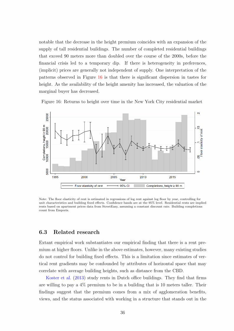
notable that the decrease in the height premium coincides with an expansion of the

supply of tall residential buildings. The number of completed residential buildings

that exceed 90 meters more than doubled over the course of the 2000s, before the

financial crisis led to a temporary dip. If there is heterogeneity in preferences,

(implicit) prices are generally not independent of supply. One interpretation of the

patterns observed in Figure 16 is that there is significant dispersion in tastes for

height. As the availability of the height amenity has increased, the valuation of the

marginal buyer has decreased.

Figure 16: Returns to height over time in the New York City residential market

Note: The floor elasticity of rent is estimated in regressions of log rent against log floor by year, controlling forunit characteristics and building fixed effects. Confidence bands are at the 95% level. Residential rents are impliedrents based on apartment prices data from StreetEasy, assuming a constant discount rate. Building completionscount from Emporis.

6.3 Related research

Extant empirical work substantiates our empirical finding that there is a rent pre-

mium at higher floors. Unlike in the above estimates, however, many existing studies

do not control for building fixed effects. This is a limitation since estimates of ver-

tical rent gradients may be confounded by attributes of horizontal space that may

correlate with average building heights, such as distance from the CBD.

Koster et al. (2013) study rents in Dutch office buildings. They find that firms

are willing to pay a 4% premium to be in a building that is 10 meters taller. Their

findings suggest that the premium comes from a mix of agglomeration benefits,

views, and the status associated with working in a structure that stands out in the

36

skyline (i.e., a ”landmark” effect). Shilton and Zaccaria (1994) and Colwell et al.

(1998) similarly find higher office rents in taller buildings. An exception in this

literature is Eichholtz et al. (2010), who find mixed results. Compared to previous

work, Liu et al. (2018) improve on the identification in that they control for building

fixed effects when estimating commercial vertical rent gradients across multiple U.S.

cities. They estimate significantly larger values of the floor elasticity of rent βC

of 0.086 within the CompStat data set and even 0.189 within the Offering memo

data set. Using the same procedure as above, we can translate these estimates into

estimates of the height elasticity of average rent ωC of 0.07 and 0.15 for buildings

up to SMAX = 40 floors.

As for residential height premiums, Wong et al. (2011) find a vertical price gra-

dient in Hong Kong apartments while Chau et al. (2007) find a price premium in

Hong Kong for those units that have a sea view. Danton and Himbert (2018) es-

timate that within buildings in Switzerland, residential rents increase by 1.5% per

floor. Their sample mostly consists of smaller structures. For the average floor of

two within their sample, the implied floor elasticity of rent βR is 0.03, somewhat less

than what we find of taller residential structures in New York City and Chicago.

Some of the more recent studies on vertical rent gradients have attempted to

identify the underlying mechanisms. In perhaps the first paper to include a measure

that controls for views, Nase et al. (2019) find that for the Amsterdam office market,

27% of the height premium is related to the view, while 70% is due to firm-level

signaling and other firm-specific factors. Liu et al. (2018) find evidence that firms in

the U.S. pay premiums not only for better amenities (views and sunlight) but also

to signal their productivity. They also document vertical sorting, with businesses

that generate higher revenues per worker, such as law firms, being located on higher

floors.

In contrast, businesses that value accessibility, such as retail, located on lower

floors, even paying a significant ground floor premium. Related to the “signaling

effect”, Dorfman et al. (2017) perform a novel behavioral study in which they explore

the perceptions of status and building height. In particular, they investigate how

people view the concept of power in regards to floor height. From their survey

analysis, they find that people perceive those residing on higher floors as being

more powerful. Ben-Shahar et al. (2007) apply a cooperative game theory model

to allocate the land and construction costs among the stories of the building. They

show how the desire for status can generate a height premium in the cost allocation

game.

Liu et al. (2020) show that the vertical employment density gradient follows the

37

vertical rent gradient, just like the horizontal density gradient follows the horizontal

rent gradient. Hence, there is a u-shaped relationship between worker density and

height, consistent with firms optimally adjusting factor inputs to factor prices.

6.4 Potential for future research

Despite recent progress, there are still relatively few studies that explore vertical rent

gradients controlling for location via building effects. In particular, the evidence is

thin for commercial buildings outside the U.S. and tall residential buildings more

generally.

There is no substantial evidence on how returns to height have changed in the

long run. In determining optimal building heights, returns to height are isomorphic

to the costs of height (see Section 4.1). Hence, in terms of rationalizing the evolution

of the urban height gradient over time, understanding changes in returns to height

is as important as understanding changes in the cost of height.

The origins of the residential vertical rent gradient have remained understudied.

Disentangling the effect of a view amenity from other height effects such as prestige

is a fairly obvious research question. Similarly, little is known about heterogeneity in

the valuation of the height amenity. Estimates of the income elasticity of the height

amenity would be informative with respect to vertical and horizontal sorting. If

richer households were willing to pay a greater height premium, tall buildings could

contribute to spatial income segregation through a preference channel, in addition

to an affordability channel.

Despite the notion that certain agglomeration effects such as knowledge spillovers

are highly localized (Rosenthal and Strange, 2001), productivity spillovers within

buildings have remained under-researched. Decades of research into horizontal ag-

glomeration effects naturally suggest that priority areas for research into vertical

spillovers should include causal estimates of the vertical within-building spillovers

after controlling for selection; the attenuation of spillovers over vertical distances;

the relative importance of information and input sharing, matching, and learning

within buildings; and the co-location benefits across industries (see Combes and

Gobillon (2015) for a recent review of the empirics of agglomeration).

7 Sticky Adjustment

So far, our analysis has been guided by a competitive equilibrium framework in

which, for given costs and returns to height, there is a direct mapping from location-

specific rents to optimal location-specific building heights. We have assumed that

38

the distribution of fundamental productivity and amenity is continuous, and the city

is perfectly malleable; hence, all gradients are “smooth”. In this section, we discuss

why, in reality, short buildings survive in central cities.

7.1 Anecdotal evidence

Recent research into the fractal dimensions of cities reveals that the shape of skylines

is more irregular than the already pretty irregular shape of city boundaries (Anas

et al., 1998; Qin et al., 2015). Economically, an irregular building height profile can

be rationalized with differences in the amenity and productivity of locations that

translate into variations in rents. Since short and tall buildings often stand side-

by-side, this explanation is not fully satisfactory. A walk down a typical block in

Lower Manhattan will reveal 19th-century low-rise buildings wedged next to 50-story

skyscrapers. At this scale, it is difficult to think of differences in fundamentals that

give rise to correspondingly large variation in rents.

To document micro-geographic variation in height more systematically, we illus-

trate the average height within one-kilometer distance-from-the-CBD bin along side

the standard deviation in heights within these bins for New York City and Chicago

in Figure 17. Even within just one kilometer from the the CBDs in New York City

and Chicago, the standard deviation in building heights is about as large as the

average height. Even with highly localized agglomeration spillovers in knowledge-

based tradable services (Arzaghi and Henderson, 2008), it is difficult to rationalize

this degree of variation in heights within such a small area. The degree of variation

in heights within bins near the CBD is all the more striking as the coefficient of

variation drops sharply after about five kilometers. Although more remote bins are

much larger, the relative variation in heights is much lower.

There are several institutional explanations for this remarkable degree of micro-

geographic variation in in downtown building heights. Land use regulations and

historic preservation are obvious candidates. New York City zoning rules, for exam-

ple, limit the amount of floor area on each block. Owners of smaller buildings with

“extra” floor area can sell it to owners of neighboring properties. They then forego

any future densification of their properties, and the result is a persistent difference

in the height of neighboring buildings.

Property rights also matter. Public ownership may deter teardowns since evicting

residents can be politically costly. As an example, municipal governments in China

typically sign 70-year land leases with residential developers. When these leases run

out in the coming decades, governments may face pressure to renew them to avoid

redevelopment and mass displacement. Large cities in the U.S. that own public

39

housing projects face similar pressures.

The protection of sitting tenants, such as under the U.S. rent control and stabi-

lization laws, implies that landlords cannot redevelop their properties if some tenants

exercise their right of lease renewals. If ownership is private but fragmented, such

as in a coop, condominium, or homeowner association, selected owners can veto the

redevelopment of a property, even if there is a clear economic case.

In addition to these institutional origins, there are some more sources of stickiness

that have received more attention in economics research and which we review below.

.

Figure 17: Variation in height

Note: Point zero n New York City is the Empire State Building. CBD in Chicago is W. Jackson Blvd. and S.Dearborn Sts. Data from the NYC PLUTO File and the Chicago Building Footprints Shapefile

7.2 Related literature

The economics literature has brought forth at least three not mutually exclusive

explanations for why the sheer scale of skyscrapers may lead to “stickiness” in ad-

justments to changing economic circumstances.

Holdouts Skyscrapers generally require large lots to make the economics work.

In dense older cities like New York, lots on a block can be owned by several owners.

A developer of a tall building then needs to assemble lots. During this process,

owners of one or two strategically-located lots may refuse to sell in an effort to extra

monopoly rents (Cunningham, 2013; Strange, 1995). This is the holdout problem.

40

To avoid this problem, developers typically buy lots in secret. Still, if a block has

many small lots with different owners, it may take years or decades even to assemble

a sufficiently large parcel for the development of a skyscraper.

Durability Tall buildings by their very nature are frequently expected to last

decades if not centuries. Beyond marginal changes, it is not economically feasible to

adjust the height of existing tall structures as this would require additional elevator

shafts and reinforcements of structural components and foundations. Brueckner

(2000) provides a summary of the standard land-use models that incorporate the

durable nature of structures. Some models assume that structures are infinitely-

lived, and new ones get added on the urban core as the city expands. Other models

assume redevelopment based on depreciation and changing prices. Henderson et al.

(2016) nicely illustrate how adding a dynamic element to the land use model can

produce “jagged” or fractal spatial structure in regard to its structural density.

Options Value An owner of a central-city vacant or under-utilized lot must decide

on the timing of construction (Williams, 1991). Because of the inherent uncertainty

and the long lag between ground breaking and opening, developers cannot always

correctly predict the revenue they will obtain upon opening. Consistent with op-

tions theory, Barr (2010) shows empirically that price uncertainty delays skyscraper

construction in Manhattan. Due to strategic interaction, option values that build up

over time are capitalized periodically, leading to waves of local development under

different fundamentals with correspondingly differing economic heights (Grenadier,

1995, 1996; Schwartz and Torous, 2007).

7.3 Potential for future research

Except for Barr (2010), there is no work that empirically explores the timing of

skyscraper construction, or how tall building durability might affect future con-

struction. In most larger, older cities, like New York and London, the vast majority

of structures were built before World War II. This suggests a tremendous lock-in

force at work once the decision to build is made. Skyscrapers rarely get torn down,

and the implications for spatial structure, agglomeration effects, and the quality

of urban life are worth exploring. Closely related, there is also scope for research

linking the increasing option value of vacant land (Barr et al., 2018) to the timing

of development, the malleability of urban spatial structure, and the cost of housing

and office space.

41

8 Geology

Intuitively, skyscrapers are so tall and heavy that they need to be stabilized in some

way so that they do not lean or deferentially settle (or fall over). This intuition

underpins the use of geological conditions as relevant instruments for density in the

identification of agglomeration spillovers (Rosenthal and Strange, 2008; Combes et

al., 2011). In this section, we review the research into geology as a determinant of

the cost of construction of tall buildings.

8.1 Related research

Deeply embedded in New York’s historiography is that skyscrapers are “missing”

between Downtown and Midtown because the bedrock in that area (which includes

Greenwich Village and the Lower East Side) is far below the surface. From a de-

tailed inspection of building heights and bedrock depths, however, Barr et al. (2011)

conclude that subsoil supply-related conditions play a much less important role for

skyscraper formation than demand for space in the two economic centers. Where

engineers encountered difficulties regarding the geological conditions, they were able

to devise innovative methods to make skyscrapers cost effective. That said, there

is some evidence that, conditional on the decision to develop a skyscraper within

Downtown, developers may have “moved” their skyscrapers to locations with more

favorable geological conditions. So, bedrock appears to be a relevant determinant

of building heights in New York at a micro-geographic level primarily.

Closely related, Barr and Tassier (2016) show that the rise of Midtown as a sepa-

rate skyscraper district was due to the agglomerative forces related to shopping and

commercial activity north of 14th Street. This commercial district emerged after

the U.S. Civil War, following the northward expansion of Manhattan’s residential

districts. Having become the natural focal point on a long and narrow island, Mid-

town was the second location after Downtown where demand drove rents above the

threshold that made skyscrapers economically viable. Taken together, Barr et al.

(2011) and Barr and Tassier (2016) demonstrate that Manhattan’s skyline shape

was driven by the demand side and not the supply side.

The evidence does not substantiate that bedrock depths are a major determi-

nant of building heights in New York. To rationalize this result, it is worth consid-

ering that Chicago, another early adopter of the skyscraper technology, was built

on “swampy soil” (Bentley and Masengarb, 2015). Thus, bedrock is not a binding

requirement for the construction of skyscrapers. Although skyscrapers are anchored

directly to the bedrock where it is easily accessible, there are relatively cost-effective

42

alternatives. Typically, if there is no bedrock near the surface, foundations are cre-

ated by boring long piles into the subsoil and then placing a concrete mat on top

of them, with the structure built on top of the mat. It is not clear that anchoring a

skyscraper to bedrock is necessarily always the cheaper alternative. As an example,

accessing bedrock in downtown Manhattan is quite difficult because on top of the

rock floor is viscous, wet quicksand with boulders scattered throughout. Engineers

had to devise expensive caisson technology in order to build foundations in lower

Manhattan (Barr, 2016). And even if establishing the foundations for a tall building

on bedrock is cheaper, the cost of stabilizing a building may not vary greatly in

height. In fact, in 1929 Manhattan foundation costs were found to be essentially

independent of height (Clark and Kingston, 1930).

8.2 Potential for future research

The role of environmental factors of the location and heights of skyscrapers remains

understudied. Recent work has looked at the role of geology on housing prices (Saiz,

2010; Burchfield et al., 2006), but there are no studies have analysed how geology

effects foundation costs since the late 19th century. Further evidence on the impact

of below-ground conditions on the cost of tall buildings from a larger sample of

cities would be useful to substantiate the case for using geology as an instrument

for agglomeration.

9 “Too Tall” Height

A profit-maximizing developer will build a structure such that at the last floor, the

marginal cost of adding that floor equals the marginal revenues. In this section, we

review the literature that has conjectured that skyscrapers, measured against this

benchmark, may be “too tall”.

9.1 Anecdotal evidence

As discussed in Sections 5 and 6, average construction costs are positively convex

in height and exceeding returns to height at the margin. Thus, at a given time and

location, there exists an optimal economic height of the building that maximizes

the profits. However, if tall buildings serve non-economic objectives, some buildings

may be too tall, in the sense that the chosen height had a marginal cost exceeds the

marginal revenue, at the time of completion.2 The debate about whether skyscrap-

2Bercea et al. (2005) argue that in the 16th century, the Roman Catholic church used cathedralsto signal their power when faced with competition from Protestantism.

43

ers, as a class of structures, or particular buildings, are too tall has a long and

contentious history, which began in New York City at the end of the 19th-century.3

In 1930, Clark and Kingston (1930) wrote their book, The Skyscraper: Study

in the Economic Height of Modern Office Buildings, to argue that those who called

skyscrapers “freak buildings,” misunderstood the economics of building tall. They

argued that tall buildings were inherently a function of high land values, and they

aimed to silence critics who felt that tall buildings were an inefficient use of land.

Nonetheless, they published their book during a famous “height race” in New

York City, at the end of the Roaring Twenties (Tauranac, 1997). In 1930, the Bank

of Manhattan (283 meters) topped out its world-record-breaking building, only to

soon be beaten by the Chrysler Building (318 meters), which within a year was

beaten by the Empire State Building (381 meters) in 1931. This race to dominate

the skyline has only fueled the perception that ego-driven developers are imposing

their will on the skyline, and the economics be damned (Barr, 2016).

There is also the perception that developers of the world’s tallest building add

extra-height to preempt would-be entrants, thus allowing the record holders to keep

their records for extra time. Supporters of this theory can point to the Empire State

Building, which held its record for 40 years. Based on the data in Figure 1, 40% of

record holders held their title for more than ten years. However, there are also cases

of rapid-fire succession. 40 Wall Street held its record for a matter of months. The

Twin Towers lost their record within a year. And the Petronas Towers (1999) (only

a record due to its spires, not its floor count) lost its record to the Taipei 101 within

five years.

More broadly, the ability to use case studies to generalize about the motivations

of record-breaking developers is limited. The reasons for building “too tall” are

multifaceted. Cities in Asia have more complex land markets and greater government

involvement in supertall projects. Skyscrapers may have additional second-order

economic benefits that can be confused for or correlated with “ego-based” height.

This can include various types of advertising or signaling, and which may come

from the builder, the occupants, the city, or the nation (Watts et al. (2007), Garza

(2017), Garza (2017)). Developers may also use their structures as “loss leaders”

to increase land values of surrounding properties and to draw income from tourism.

Observation decks in the clouds are profitable ventures.3Note that in 1893, Chicago began a half-century of capping its building heights, thus

disquali-fying itself from the debate about whether its buildings were too tall or not.

44

9.2 The Literature on Height Competition

Helsley and Strange (2008) offer a game-theoretic model of height competition. They

observe that across the world, a city’s tallest building is often much higher than the

second tallest building. They argue that if two developers are vying to claim the

prize of the “tallest building” for bragging rights or personal satisfaction (i.e., ego),

then a pure-strategy equilibrium will have one builder constructing a building so tall

it will have zero economic profit. In a mixed-strategy equilibrium, each builder will

assign a positive probability to building too tall. In a sequential game, developers

deliberately build extra tall to deter competitors. In short, they demonstrate that

“too tall” construction can be rationalized theoretically.

Prompted by this theoretical contribution, there has been some work on em-

pirically measuring the effects of height competition. However, it has remained a

challenge to separate competition effects from the effects of unobserved fundamen-

tals, so the evidence is best interpreted as suggestive.

Barr (2010) studies the economics of skyscraper construction in Manhattan using

time series data from 1895 to 2004. He estimates the economic heights and number

of completions with a regression that includes economic fundamentals. While he

cannot rule out height competition from time to time and for particular buildings,

skyscraper heights, on average, are consistent with economic fundamentals.

Barr (2012) analyses the effects of height competition by regressing the heights

of a newly-completed buildings on a weighted average of the heightsof surrounding

structures (completed before or contemporaneously). The estimate for the spatial

autoregressive parameter turns out to be positive and statistically significant, but

is economically small. Extra height is mostly added during boom times when the

forgone profits are relatively more affordable.

Barr (2013) investigates height competition between two rivaling skyscraper

cities, namely New York and Chicago. He uses time-series measures of each other

city’s skyscraper construction (average heights and completions) to estimate skyscraper

reaction functions. He finds that each city adds heights in response to the (lag of)

building activity in the other city, but, again, the interaction coefficients are eco-

nomically small.

Barr and Luo (2020) analyze skyscraper construction across Chinese cities. They

find that local GDP and population are strong predictors of skyscraper height and

completions, which suggests that China’s rapid urbanization is driving the rise of

its skylines. They also find that cities with younger officials build taller skyscrapers,

suggesting the desire to use icons for career promotion in a system where municipal

officials control land use through land leases (Brueckner et al., 2017). From spatial

45

autoregressions, they infer that same-tier cities are competing against each other in

the height market, in order to advertise their cities and its officials.

Using a different approach that draws from the spatial point-pattern literature

(Duranton and Overman, 2005), Ahlfeldt and McMillen (2015) document that the

completion of a very tall building is followed by a period of less ambitious construc-

tions in the immediate neighbourhood. While this finding is consistent with the

sequential-game predictions of the Helsley and Strange (2008) model, an existing

tall building may also lead to a lower economic height for subsequent buildings due

to a lower view amenity.

Taken together, the evidence suggests that there may be a strategic element in

height decisions, but that the effects of fundamentals dominate.

9.3 Other related research

White Elephants Gjerløw and Knutsen (2019) test the hypothesis that auto-

cratic leaders build “white elephants” as symbols of their reigns, or to demonstrate

their power to muster significant resources, or to provide work or provide incomes

to their supporters. They show that going from maximum democracy to maximum

autocracy is associated with about one extra skyscraper, ceteris paribus. They also

find that autocracies are more likely to add more “vanity height” to their structures,

where vanity height is the difference between the roof-line and the height of the top-

most part of the building. They interpret this extra height as the desire to signal

the power of autocratic leaders.

Urban Planning and Growth Anecdotally, cities world-over appear to be using

supertall buildings as catalysts of urban development and renewal. For example,

the so-called Three Brothers of Shanghai (the Jin Mao Tower, the Shanghai World

Financial Center, and the Shanghai Tower) were part of the master plan for Lujiazui

financial district. The Burj Kalifa and the Jeddah Tower (under-construction) are

central features of new neighborhoods being developed. The original Twin Towers in

New York were part of a strategy to modernize and re-invigorate lower Manhattan,

which had fallen on hard times after World War II. Unlike for sports stadia (Coates,

2007; Ahlfeldt and Kavetsos, 2014), there is no work in economics that explores how

skyscrapers induce land values, house prices, or foreign direct investment.

The skyscraper curse The so-called Skyscraper Curse alleges that supertall

building completions are a herald of economic doom (Lawrence, 1999). Support-

ers point to the Empire State Building, completed in 1931, and the Burj Khalifa,

46

completed in 2010, to show that these towers were finished during severe downturns.

Since there are about twice as many record-breaking builds than economic crises

over the past 100 years, it is relatively easy to “manually” pair record-breaking

buildings with business cycle peaks. Barr et al. (2015) are the first to rigorously test

the skyscraper curse hypothesis using Granger-causality analysis. The result is that

height cannot be used to predict the business cycles, but economic growth can be

used to forecast building heights.

9.4 Potential or future research

Each generation redefines its own “normal” building height. In the late 19th century,

15 stories was considered excessive. By the 1920s, 40 stories was not uncommon.

Today 100-story structures are regularly built. As the barriers to building height

continue to fall away, the debate about whether skyscrapers are too tall keeps re-

newing itself.

Empirical research into whether the tallest structures in the world are, in fact,

economically too tall remains challenging due to data limitations. Thus far, com-

prehensive data that are readily accessible are confined to completed heights of

buildings and the general economic climate in which they are built. Building-level

data on revenues and the costs of land acquisition and construction cost will be key

to evaluating the economic case for building super-tall.

Since skyscrapers are durable and there are significant construction lags, expec-

tations matter for building height decisions. Seemingly excessive structures may

be result of perfectly foreseen economic growth or a myopically extrapolated real

estate boom. Understanding the extent to which cyclical vertical growth can be

rationalized under perfect foresight may be informative with respect to the role of

expectations on real estate markets more generally.

10 Regulation and externalities

In this section, we review the literature on causes and effects of regulation that seeks

to address external effects skyscraper may have on their cities and neighbourhoods.

10.1 Anecdotal evidence

When tall buildings started to rise in U.S. cities at the end of the 19th century,

planners and officials were concerned about shadows, increased traffic congestion,

increased risk of conflagrations, and correspondingly reduced property values of

surrounding buildings (Heights of Buildings Commission, 1913; Hoxie, 1915).

47

While some cities, like Chicago and Boston, placed direct height caps on their

buildings, New York never did. In 1916, it implemented the first comprehensive

zoning regulations in the nation. Rather than capping heights, it mandated setback

rules that required tall buildings to set back from the street line as they rose taller.

This gave rise to the so-called “wedding-cake style” architecture. The purpose of

this regulation was to increase sunlight on the streets and reduce total building area

and congestion. New York’s codes were widely copied throughout the country in the

1920s (Weiss, 1992). These policies were not based on rigorous social cost-benefit

analyses. Instead, planners followed their own normative judgements under the

constraint that the imposed regulation should not be overturned by courts (Weiss,

1992; Bertaud, 2018).

Today, cities around the world generally attempt to control building height and

density by capping the maximum allowable floor area ratios (FARs). The FAR is

the total building area divided by the lot area. For example, the maximum allowable

FAR for Manhattan office buildings is 15 (or 18 if open space is provided). Similarly,

for Chicago, the maximum FAR is 12. To put these numbers in perspective, the

maximum FAR for Paris, a “flat” city, is 3 (Brueckner and Sridhar, 2012).

In keeping with intuition, Figure 18 shows a positive correlation between max-

imum allowable central-city FARs on the one hand, and the number and height

of skyscrapers on the other, for cities around the world. The relationship, how-

ever, is quite noisy, suggesting that the causes and effects of regulation of vertical

growth are highly context-dependent. As an example, the most vertical cities of the

world, Hong Kong and New York have many and tall skyscrapers despite the FAR

regulation being more restrictive than in Tokyo or Singapore.

10.2 Related research

Gyourko and Molloy (2015) provide a review of a sizable literature on the causes and

effects of effects of building regulation. The literature specifically concerned with

height regulation is somewhat thinner but growing.

In general, it appears that FAR regulation tends to be binding. In several anal-

yses, Barr (2010, 2012, 2013) concludes that zoning regulations in New York and

Chicago reduce building heights. Ahlfeldt and McMillen (2018) find that in Chicago,

the building footprints of taller buildings cover a smaller fraction of the land par-

cel. This relationship reflects that for developers to go tall, they must reduce the

floor plate sizes in order to maintain the maximum allowable FAR. Sometimes, ex-

tra height is allowed in return for publicly accessible open space, further reducing

the floor plate. Theoretically, the partial equilibrium effect of a forced reduction in

48

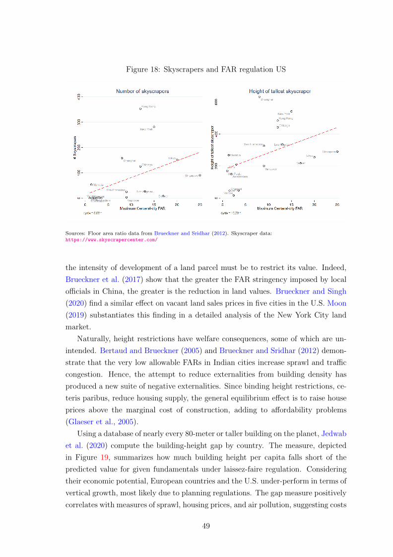
Figure 18: Skyscrapers and FAR regulation US

Sources: Floor area ratio data from Brueckner and Sridhar (2012). Skyscraper data:https://www.skyscrapercenter.com/

the intensity of development of a land parcel must be to restrict its value. Indeed,

Brueckner et al. (2017) show that the greater the FAR stringency imposed by local

officials in China, the greater is the reduction in land values. Brueckner and Singh

(2020) find a similar effect on vacant land sales prices in five cities in the U.S. Moon

(2019) substantiates this finding in a detailed analysis of the New York City land

market.

Naturally, height restrictions have welfare consequences, some of which are un-

intended. Bertaud and Brueckner (2005) and Brueckner and Sridhar (2012) demon-

strate that the very low allowable FARs in Indian cities increase sprawl and traffic

congestion. Hence, the attempt to reduce externalities from building density has

produced a new suite of negative externalities. Since binding height restrictions, ce-

teris paribus, reduce housing supply, the general equilibrium effect is to raise house

prices above the marginal cost of construction, adding to affordability problems

(Glaeser et al., 2005).

Using a database of nearly every 80-meter or taller building on the planet, Jedwab

et al. (2020) compute the building-height gap by country. The measure, depicted

in Figure 19, summarizes how much building height per capita falls short of the

predicted value for given fundamentals under laissez-faire regulation. Considering

their economic potential, European countries and the U.S. under-perform in terms of

vertical growth, most likely due to planning regulations. The gap measure positively

correlates with measures of sprawl, housing prices, and air pollution, suggesting costs

49

of regulation.

Figure 19: Per-capita height gaps by country

Note: The height gap measures by how much total height of tall buildings in per-capita terms falls short of thepredicted value under laissez-fair regulation (for given fundamentals). The measure is constructed for 149 countriesin 2020. Positive values (red shades) indicate more stringent regulation. Source: Jedwab et al. (2020).

In some cities, planners seek to mitigate negative externalities by ensuring that

tall buildings are aesthetically appealing. Cheshire and Dericks (2020) study the

impact of tight building height regulations in London, where skyscrapers have to go

through an approval process since there is no “as-of-right“ development as in New

York or Chicago. The authors document that developers employing so-called Tro-

phy Architects—those that won one of three prestigious architectural awards—are

allowed to build 14-floors taller than otherwise, a sizable magnitude in a reasonably

flat city. They interpret the one-and-a-half-fold increase in site value due to the

extra permitted height as the compensation of the cost of rent-seeking and, thus, an

indirect measure of dead-weight loss.

Ironically, some of the unintended negative effects of height restrictions may

have socially desirable second-order effects. Borck (2016) shows theoretically how

building height regulation leads to lower housing consumption due to a supply-driven

increase in house prices, which leads to a reduction in greenhouse gas emissions. In

his model with a global emissions externality, the welfare effect is non-monotonic

and, depending on the value of the externality, either the absence of height regulation

or a very stringent regulation can be socially desirable.

50

10.3 Potential for future research

Much of the literature on height regulation is concerned with the negative collateral

effects. One naturally wonders how these costs compare to potential benefits that

motivate height regulations in the first instance. There is some evidence pointing to

amenity values of sunshine (Fleming et al., 2018) and distinctive design (Ahlfeldt and

Holman, 2018), suggesting that a regulation that reducse shadowing and improves

the design of tall buildings may have positive effects. Also, while very tall buildings

likely reduce sprawl and encourage mass transit, they tend to produce more CO2 on

per square meter, so that their environmental impact is theoretically ambiguous.

There is an evident polarization between opponents and proponents of tall build-

ings. The former argue that skyscrapers are, aesthetically speaking, “too big” for

the “human scale” (Gehl, 2013) and an anathema to the vibrant city that Jason

Jacobs (1961) argued for. The latter focus on the cost of height restrictions that

materialize in sprawl and affordability problems. Yet, only a quantitative evalua-

tion of the positive and negative external effects of tall buildings enables setting

the appropriate Pigovian tax for a transition into a first-best optimum of building

heights.

Likely, the degree of stringency of height regulation varies significantly across

cities around the world because the external costs and benefits vary, too. Develop-

ing an understanding of external costs and benefits of skyscrapers that account of

heterogeneity across institutional context is an ambitious research agenda that will

likely remain topical for quite some time.

11 Conclusion

The high-level conclusion of our synthesis is that the literature engaging with the

economics of tall buildings is still at an early stage. We have discussed the potential

for future research throughout Sections 4 to 10. Below, we offer an admittedly

subjective selection of three priority areas for research into the vertical dimension of

cities.

First, there is a long way to go in understanding how the positive and negative

externalities associated with tall buildings play out on balance. Skyscrapers may

not just accommodate productive workers in productive locations but also facilitate

gains in productivity, ceteris paribus, if the vertical cost of interaction is sufficiently

low. If well-designed skyscrapers put neighbourhoods or cities on the map, they

may attract businesses and tourism. At this same time, skyscrapers may generate

external costs in the form of shadowing, congestion, or the loss of a coherent historic

51

fabric.

Second, there is scope for exploring the costs of and returns to height more

fully. Costs of and returns to height appear to be non-linear, and there are likely

threshold effects that could be explored with richer data sets. Heterogeneity in the

cost of height across uses and the value of the height amenities across users is not

only interesting in its own right but also has implications for the horizontal pattern

of land use and sorting. The net cost of height is one of the main congestive forces

and a better understanding of how it evolves over time is helpful with respect to

rationalizing changes in the spatial structure in the past as well as anticipating the

evolution of cities in the future.

Third, there are forces outside the canonical competitive equilibrium framework

that shape the urban height profile and deserve more attention. As an example,

disentangling the effects of height competition from fundamentals that would jus-

tify extreme building heights remains an empirical challenge. Progress on this front

will be essential for economically rationalizing skyscrapers such as the Empire State

Building or the Burj Khalifa, which dominate height rankings for decades and ex-

emplify the frontier of technological innovation and human ambition.

52

References

Abdel-Wahab, Mohamed and Bernard Vogl, “Trends of productivity growthin the construction industry across Europe, US and Japan,” Construction man-agement and economics, 2011, 29 (6), 635–644.

Ahlfeldt, Gabriel M. and Daniel P. McMillen, “Land Values in Chicago,1913–2010: A Cityas Spatial History Revealed,” Land Lines, 2014, (April).

and , “New estimates of the elasticity of substitution between land and capi-tal,” Working paper, 2014.

and , “The vertical city: the price of land and the height of buildings inChicago 1870-2010,” SERC discussion paper, 2015, 180.

and , “Tall buildings and land values: Height and construction cost elasticitiesin Chicago, 1870-2010,” Review of Economics and Statistics, 2018, 100 (5), 861–875.

and Elisabetta Pietrostefani, “The economic effects of density: A synthesis,”Journal of Urban Economics, 5 2019, 111, 93–107.

and Georgios Kavetsos, “Form or function? The effect of new sports stadiaon property prices in London,” Journal of the Royal Statistical Society. Series A:Statistics in Society, 2014, 177 (1).

and Nancy Holman, “Distinctively Different: A New Approach to ValuingArchitectural Amenities,” The Economic Journal, 9 2018, 128 (608), 1–33.

and Nicolai Wendland, “Fifty years of urban accessibility: The impact of theurban railway network on the land gradient in Berlin 1890-1936,” Regional Scienceand Urban Economics, 2011, 41 (2).

, Stephen J. Redding, Daniel M. Sturm, and Nikolaus. Wolf, “The Eco-nomics of Density : Evidence from the Berlin Wall,” Econometrica, 2015, 83 (4).

, Thilo Albers, and Kristian Behrens, “Prime locations,” Working paper,2020.

Al-Kodmany, Kheir, “Tall buildings and elevators: A review of recent technolog-ical advances,” Buildings, 2015, 5 (3), 1070–1104.

and Mir M Ali, The future of the city: Tall buildings and urban design, WITpress, 2013.

Ali, Mir M and Kyoung Sun Moon, “Structural developments in tall buildings:current trends and future prospects,” Architectural science review, 2007, 50 (3),205–223.

Alonso, William, Location and Land Use, Cambridge, MA: Harvard Univ. Press,1964.

53

Anas, Alex, Richard Arnott, and Kenneth A Small, “Urban spatial struc-ture,” Journal of economic literature, 1998, 36 (3), 1426–1464.

Arzaghi, Mohammad and J Vernon Henderson, “Networking off MadisonAvenue,” The Review of Economic Studies, 10 2008, 75 (4), 1011–1038.

Baker, William, “Building Systems and Concepts - Structural Innovation,” in“Conference Proceedings of the 6th World Congress of the CTBUH,” Council onTall Buildings and the Urban Habitat, 2001, pp. 481–493.

Barr, Jason, “Skyscrapers and the Skyline: Manhattan, 1895–2004,” Real EstateEconomics, 2010, 38 (3), 567–597.

, “Skyscraper Height,” Journal of Real Estate Finance and Economics, 2012, 45(3).

, “Skyscrapers and Skylines: New York and Chicago, 1885-2007,” Journal ofRegional Science, 2013, 53 (3).

, Building the Skyline: The Birth and Growth of Manhattan’s Skyscrapers, OxfordUniversity Press, 2016.

and Jeffrey P Cohen, “The Floor Area Ratio Gradient: New York City, 1890-2009,” Regional Science and Urban Economics, 2014, 48, 110–119.

and Jennifer Johnson, “Skyscrapers and the happiness of cities,” EasternEconomic Journal, 2020, 46 (2).

and Jingshu Luo, “Growing Skylines: The Economic Determinants of Skyscrap-ers in China,” The Journal of Real Estate Finance and Economics, 2020.

and Troy Tassier, “The Dynamics of Subcenter Formation: Midtown Manhat-tan, 1861–1906,” Journal of Regional Science, 2016, 56 (5), 754–791.

, Bruce Mizrach, and Kusum Mundra, “Skyscraper height and the businesscycle: separating myth from reality,” Applied Economics, 2015, 47 (2).

, Fred Smith, and Sayali Kulkarni, “What’s Manhattan worth? A land valuesindex from 1950 to 2014,” Regional Science and Urban Economics, 2018, 70.

, Troy Tassier, and Rossen Trendafilov, “Depth to Bedrock and the Forma-tion of the Manhattan Skyline, 1890–1915,” The Journal of Economic History,2011, 71 (4), 1060–1077.

Baum-Snow, Nathaniel, “Did Highways Cause Suburbanization?,” The QuarterlyJournal of Economics, 2007, 122 (2), 775–805.

and Lu Han, “The Microgeography of Housing Supply,” Working paper, 2019.

, Loren Brandt, J Vernon Henderson, Matthew A Turner, and QinghuaZhang, “Roads, Railroads, and Decentralization of Chinese Cities,” The Reviewof Economics and Statistics, 1 2017, 99 (3), 435–448.

54

Ben-Shahar, Danny, Yonghen Deng, and Eyal Sulganik, “Shapley cost allo-cation coincides with relative status: The case of skyscrapers,” 2007.

Bentley, Chris and Jennifer Masengarb, “Building Skyscrapers on ChicagoasSwampy Soil,” 2015.

Bercea, Brighita, Robert B Ekelund Jr., and Robert D Tollison, “Cathedralbuilding as an entry-deterring device,” Kyklos, 11 2005, 58 (4), 453–465.

Bertaud, Alain, Order without design: How markets shape cities, Mit Press, 2018.

and Jan Brueckner, “Analyzing building-height restrictions: predicted impactsand welfare costs,” Regional Science and Urban Economics, 2005, 35 (2), 109–125.

Borck, Rainald, “Will skyscrapers save the planet? Building height limits andurban greenhouse gas emissions,” Regional Science and Urban Economics, 2016,58, 13–25.

Brooks, Leah and Byron Lutz, “Vestiges of Transit: Urban Persistence at aMicroscale,” The Review of Economics and Statistics, 3 2019, 101 (3), 385–399.

Brueckner, Jan, “The structure of urban equilibria: A unified treatment of themuth-mills model,” Handbook of Regional and Urban Economics, 1 1987, 2, 821–845.

, “Urban growth models with durable housing: An overview,” in Jean-Marie Hu-riot Huriot and Thisse Jacques-FranA§ois, eds., Economics of Cities: TheoreticalPerspectives, Cambridge University Press Cambridge, 2000, chapter 7, pp. 263–289.

and Kala Seetharam Sridhar, “Measuring welfare gains from relaxation ofland-use restrictions: The case of India’s building-height limits,” Regional Scienceand Urban Economics, 2012, 42 (6), 1061–1067.

and Ruchi Singh, “Stringency of land-use regulation: Building heights in UScities,” Journal of Urban Economics, 2020, 116.

and Stuart S. Rosenthal, “Gentrification and Neighborhood Housing Cy-cles: Will America’s Future Downtowns Be Rich?,” The Review of Economicsand Statistics, 10 2009, 91 (4), 725–743.

, Shihe Fu, Yizhen Gu, and Junfu Zhang, “Measuring the stringency of landuse regulation: The case of China’s building height limits,” Review of Economicsand Statistics, 2017, 99 (4), 663–677.

Burchfield, Marcy, Henry G Overman, Diego Puga, and Matthew ATurner, “Causes of sprawl: A portrait from space,” The Quarterly Journal ofEconomics, 2006, 121 (2), 587–633.

55

Chau, K W and A Walker, “The measurement of total factor productivity ofthe Hong Kong construction industry,” Construction management and economics,1988, 6 (3), 209–224.

, S K Wong, Y Yau, and AKC Yeung, “Determining optimal building height,”Urban Studies, 2007, 44 (3), 591–607.

, S W Poon, Y S Wang, and L L Lu, “Technological progress and theproductive efficiency of construction firms in Hong Kong, 1981–2001,” Journal ofConstruction Research, 2005, 6 (02), 195–207.

Cheshire, Paul C and Gerard H Dericks, “aTrophy Architectsa and Designas Rent-seeking: Quantifying Deadweight Losses in a Tightly Regulated OfficeMarket,” Economica, 2020.

Clark, William Clifford and John Lyndhurst Kingston, The Skyscraper:Study in the Economic Height of Modern Office Buildings, American Instituteof Steel, 1930.

Coates, Dennis, “Stadiums and arenas: Economic development or economic re-distribution?,” Contemporary Economic Policy, 2007, 25 (4), 565–577.

Colwell, Peter F, Henry J Munneke, and Joseph W Trefzger, “Chicago’sOffice Market: Price Indices, Location and Time,” Real Estate Economics, 3 1998,26 (1), 83–106.

Combes, Pierre-Philippe and Laurent Gobillon, “Chapter 5 - The Empiricsof Agglomeration Economies,” in Gilles Duranton, J Vernon Henderson, WilliamC B T Handbook of Regional Strange, and Urban Economics, eds., Handbook ofRegional and Urban Economics, Vol. 5, Elsevier, 2015, pp. 247–348.

, Gilles Duranton, and Laurent Gobillon, “The identification of agglomera-tion economies,” Journal of economic geography, 2011, 11 (2), 253–266.

, , and , “The Production Function for Housing: Evidence from France,”Working paper, 2016.

, , and , “The Costs of Agglomeration: House and Land Prices in FrenchCities,” The Review of Economic Studies, 10 2018, 86 (4), 1556–1589.

, , , and Sebastien Roux, “Estimating Agglomeration Economies WithHistory, Geology, and Worker Effects,” in “Agglomeration Economics,” Chicago:University of Chicago Press, 2010, pp. 15–66.

Condit, Carl W, “The two centuries of technical evolution underlying theSkyscraper,” in “Second Century of the Skyscraper,” 11–24, 1988, pp. 11–24.

Cunningham, Chris, “Estimating the holdout problem in land assembly,” 2013.

Curci, Federico, “Vertical and horizontal cities: in which direction should citiesgrow?,” Working paper, 2017.

56

, “The taller the better? Agglomeration determinants and urban structure,”Working paper, 2020.

Danton, Jayson and Alexander Himbert, “Residential vertical rent curves,”Journal of Urban Economics, 2018, 107, 89–100.

Department of the Environment, Local Authority Offices: Areas and Costs,London: DOE, 1971.

Dorfman, Anna, Danny Ben-Shahar, and Daniel Heller, “Power and highstories,” 2017.

Douglas, George H, Skyscrapers: A social history of the very tall building inAmerica, McFarland, 2004.

Duranton, Gilles and Henry G Overman, “Testing for localization using micro-geographic data,” Review of economic studies, 2005, 72 (4), 1077–1106.

Eichholtz, Piet, Nils Kok, and John M Quigley, “Doing well by doing good?Green office buildings,” The American Economic Review, 2010, 100 (5), 2492–2509.

Epple, Dennis, Brett Gordon, and Holger Sieg, “A New Approach to Esti-mating the Production Function for Housing,” American Economic Review, 2010,100 (3), 905–924.

Fleming, David, Arthur Grimes, Laurent Lebreton, David Mare, andPeter Nunns, “Valuing sunshine,” Regional Science and Urban Economics, 2018,68, 268–276.

Fujita, Masahisa and Hideaki Ogawa, “Multiple equilibria and structural tran-sition of non-monocentric urban configurations,” Regional Science and Urban Eco-nomics, 1982, 12 (2), 161–196.

Garza, Nestor, “Skyscrapers in Santiago: 300 meters of globalization agenda,”Journal of Property Investment & Finance, 2017, 35 (5), 439–454.

Gehl, Jan, Cities for people, Island press, 2013.

Gjerløw, Haakon and Carl Henrik Knutsen, “TRENDS: Leaders, Private In-terests, and Socially Wasteful Projects: Skyscrapers in Democracies and Autoc-racies,” Political Research Quarterly, 2019, 72 (2), 504–520.

Glaeser, Edward, “A nation of gamblers: Real estate speculation and Americanhistory,” American Economic Review, 2013, 103 (3), 1–42.

, Jed Kolko, and Albert Saiz, “Consumer city,” Journal of Economic Geog-raphy, 1 2001, 1 (1), 27–50.

, Joseph Gyourko, and Raven Saks, “Why Is Manhattan So Expensive?Regulation and the Rise in Housing Prices,” The Journal of Law and Economics,10 2005, 48 (2), 331–369.

57

Gort, Michael, Jeremy Greenwood, and Peter Rupert, “Measuring the rateof technological progress in structures,” Review of Economic Dynamics, 1999, 2(1), 207–230.

Grenadier, Steven R, “The persistence of real estate cycles,” The Journal of RealEstate Finance and Economics, 1995, 10 (2), 95–119.

, “The strategic exercise of options: Development cascades and overbuilding inreal estate markets,” The Journal of Finance, 1996, 51 (5), 1653–1679.

Grimaud, A, “Agglomeration economies and building height,” Journal of UrbanEconomics, 1989, 25 (1), 17–31.

Gyourko, Joseph and Raven Molloy, “Regulation and housing supply,” in“Handbook of regional and urban economics,” Vol. 5, Elsevier, 2015, pp. 1289–1337.

Heights of Buildings Commission, “Report of the Heights of Buildings Com-mission to the Committee on the Height, Size and Arrangement of Buildings ofthe Board of Estimate and Apportionment of the City of New York,” TechnicalReport, Heights of Buildings Commission, New York 1913.

Helsley, Robert W. and William C. Strange, “Urban interactions and spatialstructure,” Journal of Economic Geography, 1 2007, 7 (2), 119–138.

and , “A game-theoretic analysis of skyscrapers,” Journal of Urban Economics,7 2008, 64 (1), 49–64.

Henderson, J Vernon and Arindam Mitra, “The new urban landscape: Devel-opers and edge cities,” Regional Science and Urban Economics, 1996, 26 (6 SPEC.ISS.), 613–643.

, Tanner Regan, and Anthony Venables, “Building the city: urban transitionand institutional frictions,” CEPR Discussion Paper, 2016, 11211.

Hoxie, George L, “City taxation and skyscraper control,” Journal of PoliticalEconomy, 1915, 23 (2), 166–176.

Jacobs, Jane, The death and life of great American cities, Random House, 1961.

Jedwab, Remi, Jason Barr, and Jan Brueckner, “Cities without Skylines:Worldwide Building-height Gaps and their Implications,” 2020.

Koster, Hans R A, Jos van Ommeren, and Piet Rietveld, “Is the sky thelimit? High-rise buildings and office rents,” Journal of Economic Geography, 52013, 14 (1), 125–153.

Lago, Alberto, Hadi Moghadasi Faridani, and Dario Trabucco, “DampingTechnologies for Tall Buildings.,” CTBUH Journal, 2018, (3).

58

Larson, Gerald R and Roula Mouroudellis Geraniotis, “Toward a betterunderstanding of the evolution of the iron skeleton frame in Chicago,” The Journalof the Society of Architectural Historians, 1987, 46 (1), 39–48.

Lawrence, Andrew, “The Curse Bites: Skyscraper Index Strikes,” Technical Re-port 1999.

Lee, Jong-San, Hyun-Soo Lee, and Moon-Seo Park, “Schematic cost esti-mating model for super tall buildings using a high-rise premium ratio TA - ı´ı¢ı°TA - ı´ıı TA - e°e¬¸ı,′′ 52011.

Lee, Sanghoon and Jeffrey Lin, “Natural Amenities, Neighbourhood Dynamics,and Persistence in the Spatial Distribution of Income,” The Review of EconomicStudies, 3 2017, 85 (1), 663–694.

Liu, Crocker, Stuart S. Rosenthal, and William C. Strange, “The VerticalCity: Rent Gradients and Spatial Structure,” Journal of Urban Economics, 2018,106, 101–122.

, , and , “Employment Density and Agglomeration Economies in Tall Build-ings,” Regional Science and Urban Economics, 2020, forthcomin.

Lucas, Robert E Jr. and Esteban Rossi-Hansberg, “On the Internal Structureof Cities Author,” Econometrica, 2002, 70 (4), 1445–1476.

Malthus, Thomas Robert, An Essay on the Principle of Population, London: J.Johnson, 1798.

McDonald, John F, “Econometric studies of urban population density: A survey,”Journal of Urban Economics, 1989, 26 (3), 361–385.

McMillen, Daniel P., “One Hundred Fifty Years of Land Values in Chicago: ANonparametric Approach,” Journal of Urban Economics, 7 1996, 40 (1), 100–124.

Michaels, Guy, Ferdinand Rauch, and Stephen J. Redding, “Task spe-cialization in US cities from 1880 to 2000,” Journal of the European EconomicAssocation, 2018, forthcomin (August), 1–45.

Mills, Edwin S, “An Aggregative Model of Resource Allocation in a MetropolitanArea,” The American Economic Review, 1967, 57 (2), 197–210.

Moon, Byunggeor, “The effect of FAR (floor area ratio) regulations on land values:The case of New York,” Papers in Regional Science, 2019, 98 (6), 2343–2354.

Moretti, Enrico, The new geography of jobs, Houghton Mifflin Harcourt, 2012.

Muth, R., Cities and Housing, Chicago: Chicago University Press, 1969.

Nase, Ilir, Nick van Assendelft, and Hilde Remøy, “Rent Premiums andVertical Sorting in Amsterdamas Multi-Tenant Office Buildings,” The Journal ofReal Estate Finance and Economics, 2019, 59 (3), 419–460.

59

Picken, David and Benedict Ilozor, “The Relationship between Building Heightand Construction Costs,” 3 2015.

Qin, Jing, Chuanglin Fang, Yang Wang, Guangdong Li, and ShaojianWang, “Evaluation of three-dimensional urban expansion: A case study ofYangzhou City, Jiangsu Province, China,” Chinese geographical science, 2015,25 (2), 224–236.

Ricardo, David, On the Principles of Political Economy and Taxation, London:John Murray, 1817.

Rosenthal, Stuart S. and William C. Strange, “The Determinants of Agglom-eration,” Journal of Urban Economics, 2001, 50 (2), 191–229.

and , “The attenuation of human capital spillovers,” Journal of Urban Eco-nomics, 2008, 64 (2), 373–389.

Saiz, Albert, “The geographic determinants of housing supply,” The QuarterlyJournal of Economics, 2010, 125 (3), 1253–1296.

Schwartz, Eduardo S. and Walter N. Torous, “Commercial office space: testingthe implications of real options models with competitive interactions,” Real EstateEconomics, 2007, 35 (1), 1–20.

Shilton, Leon and Anthony Zaccaria, “The avenue effect, landmark externali-ties, and cubic transformation: Manhattan office valuation,” The Journal of RealEstate Finance and Economics, 1994, 8 (2), 151–165.

Shultz, Earl and Walter Simmons, Offices in the Sky, Bobbs-Merrill, 1959.

Smith, Adam, The wealth of nations, London: W. Strahan and T. Cadell, 1776.

Smith, Brian, Mital Dholakia, and Richard Heseltine, “Cost Model: TallBuildings,” Building, 2014, April 15.

Spengler, Edwin H, Land values in New York in relation to transit facilities,Columbia University Press, 1930.

Strange, William C., “Information, holdouts, and land assembly,” Journal ofurban Economics, 1995, 38 (3), 317–332.

Sullivan, Arthur M, “Tall buildings on cheap land: Building heights and intra-building travel costs,” Journal of Urban Economics, 1991, 29 (3), 310–328.

Tan, Willie, “Construction cost and building height,” Construction Managementand Economics, 3 1999, 17 (2), 129–132.

Tauranac, John, Empire State Building: The Making of a Landmark, Macmillan,1997.

60

von Thuenen, Johann Heinrich, Der isoli[e]rte Staat in Beziehung auf Land-wirtschaft und Nationalokonomie, oder Untersuchungen uber den Einfluß, dendie Getreidepreise, der Reichthum des Bodens und die Abgaben auf den Ackerbauausuben., Hamburg: Verlag von Wiegandt,, 1826.

Wang, Xueqing, Yuan Chen, Bingsheng Liu, Yinghua Shen, and Hui Sun,“A total factor productivity measure for the construction industry and analysisof its spatial difference: A case study in China,” Construction management andeconomics, 2013, 31 (10), 1059–1071.

Watts, Steve, Neal Kalita, and Michael Maclean, “The economics of super-tall towers,” The Structural Design of Tall and Special Buildings, 2007, 16 (4),457–470.

Weiss, Marc A, “Skyscraper zoning: New York’s pioneering role,” Journal of theAmerican Planning Association, 1992, 58 (2), 201–212.

Williams, Joseph T, “Real estate development as an option,” The Journal of RealEstate Finance and Economics, 1991, 4 (2), 191–208.

Wong, S K, K W Chau, Y Yau, and A K C Cheung, “Property pricegradients: the vertical dimension,” Journal of Housing and the Built Environment,2011, 26 (1), 33–45.

Xia, Jun, Dennis Poon, and Douglas C Mass, “Case Study: Shanghai Tower,”CTBUH Journal, 2010, (2), 12–18.

Zhi, Mao, Goh Bee Hua, Shou Qing Wang, and George Ofori, “Totalfactor productivity growth accounting in the construction industry of Singapore,”Construction management and economics, 2003, 21 (7), 707–718.

61

A1 Online appendix

This online appendix contain supplementary material not intended for publication.

A1.1 Parametrization

In this section, we provide additional detail on the parametrization of the theoretical

model introduced in 4.1.

Residential use Consider homogeneous residents that maximize the Cobb-Douglas

utility

U = ARXαRF 1−αR

subject to the budget constraint

y = pRF + C,

where AR is a location-specific residential utility shifter, C is a tradable good

with a price normalized to unity, F is floor space, pR is the residential floor space

price, and αR is the expenditure share on floor space. Using the Marshallian demand

functions C = αRy, F = (1−αR)ypR

and imposing that the spatial equilibrium anchors

indirect utility to an exogenous reservation level U = 1, the residential bid rent is

defined as:

pR = aR(AR)1

1−αR ,

where aR = (1 − αR)(αR)αR

1−αR y1

1−αR is a scale parameter that collects some

constants.

Commercial use Consider homogeneous firms that produce according to the fol-

lowing production function

X = ACKαCF 1−αC

and maximize profits

π = X − pCF −K,

where AC is a location-specific commercial productivity shifter, X is a tradable

62

good with a price normalized to unity, K is tradable capital with a price normalized

to unity, and pC is the commercial floor space price. Using the marginal rate of sub-

stitution KF

= αC

1−αC pC and assuming zero economic profits in a perfectly competitive

market, the commercial bid rent is defined as

pC = aC(AC)1

1−αC ,

where aC = (1− αC)(αC)αC

1−αC is a scale parameter that collects some constants.

Bid rent In the below we index use by U ∈ R,C for convenience and assume that

productivity and amenity decrease in distance from the CBD D:

AU = bue−τUD

so that

pU = aU(bu)1

1−αU e− τU

1−αUD,

where bu > 0 is a constant that determines the amenity level at the central point.

Developers We define height SU = FU

Las the ratio of floor space FU over the

land L occupied by a building at any location. Homogeneous developers choose SU

to maximize profits

πU(SU) = pUSU − cUSU − 1

dUrU ,

where the average rent pU = pUSUωU

and the average cost cU = cUSUθU

increase

in height at the elasticities ωU > 0 and θU > 0. dU = 1 is the fraction of a parcel

that is developable, which along with the land rent rU determines the land cost.

Profit maximization delivers the economic height

SU∗

= fU(cU)1

ωU−θU eτU

(1−αU )(ωU−θU ) ,

where fU = (aU)− 1

ωU−θU (bU)− 1

(1−αU )(ωU−θU )(

1+θU

1+ωU

) 1

ωU−θU collects various constants.

63

Land rent Using SU∗

in the developer profit function and assuming zero profits

due to perfect competition delivers the residential land rent.

rU = dU[aU(bU)

11−α (fU)1+ωU (cU)

1+ωU

ωU−θU d(1+ωU )−(ωU−θU )

(1−αU )(ωU−θU )τUD

− cU(fU)1+θU (cU)1+θU

ωU−θU e(1+θU )

(1−αU )(ωU−θU )τUD]

64

CENTRE FOR ECONOMIC PERFORMANCE Recent Discussion Papers

1703 Luke Milsom Vladimír Pažitka Isabelle Roland Dariusz Wójcik

Gravity in International Finance: Evidence from Fees on Equity Transactions

1702 Jonathan Colmer Dajun Lin Siying Liu Jay Shimshack

Why are Pollution Damages Lower in Developed Countries? Insights from High Income, High-Pollution Hong Kong

1701 Paul Cheshire Katerina Kaimakamis

Offices Scarce but Housing Scarcer: Estimating the Premium for London Office Conversions

1700 Francesco Campo Mariapia Mendola Andrea Morrison Gianmarco Ottaviano

Immigrant Inventors and Diversity in the Age of Mass Migration

1699 Mariana Spatareanu Vlad Manole Ali Kabiri Isabelle Roland

Bank Default Risk Propagation along Supply Chains: Evidence from the U.K.

1698 Georg Graetz Björn Öckert Oskar Nordström Skans

Family Background and the Responses to Higher SAT Scores

1697 Federico Cingano Fadi Hassan

International Financial Flows and Misallocation

1696 Piero Montebruno Disrupted Schooling: Impacts on Achievement from the Chilean School Occupations

1695 Ester Faia Sébastien Laffitte Maximilian Mayer Gianmarco Ottaviano

Automation, Globalization and Vanishing Jobs: A Labor Market Sorting View

1694 Ulrich J. Eberle Damned by Dams? Infrastructure and Conflict

1693 Abel Brodeur Andrew E. Clark Sarah Flèche Nattavudh Powdthavee

COVID-19, Lockdowns and Well-Being: Evidence from Google Trends

1692 Fabrice Defever José-Daniel Reyes Alejandro Riaño Gonzalo Varela

All These Worlds are Yours, Except India: The Effectiveness of Cash Subsidies to Export in Nepal

1691 Adam Altmejd Andrés Barrios-Fernández Marin Drlje Joshua Goodman Michael Hurwitz Dejan Kovac Christine Mulhern Christopher Neilson Jonathan Smith

O Brother, Where Start Thou? Sibling Spillovers on College and Major Choice in Four Countries

1690 Michael Amior Alan Manning

Monopsony and the Wage Effects of Migration

1689 Frank Pisch Managing Global Production: Theory and Evidence from Just-in-Time Supply Chains

1688 Barbara Petrongolo Maddalena Ronchi

A Survey of Gender Gaps through the Lens of the Industry Structure and Local Labor Markets

1687 Nick Jacob Giordano Mion

On the Productivity Advantage of Cities

1686 Andrew E. Clark Anthony Lepinteur

A Natural Experiment on Job Insecurity and Fertility in France

The Centre for Economic Performance Publications Unit Tel: +44 (0)20 7955 7673 Email info@cep.lse.ac.uk Website: http://cep.lse.ac.uk Twitter: @CEP_LSE