ISSN 2042-2695

CEP Discussion Paper No 1635

July 2019

Dirty Density: Air Quality and the Density of

American Cities

Felipe Carozzi

Sefi Roth

Abstract We study whether urban density affects the exposure of city dwellers to ambient air pollution using

satellite-derived measures of air quality for the contiguous United States. For identification, we rely on an instrumental variable strategy, which induces exogenous variation in density without affecting pollution directly. For this purpose, we use three variables measuring geological characteristics as instruments for density: earthquake risks, soil drainage capacity and the presence of aquifers. We find a positive and statistically significant pollution-density elasticity of 0.13. We also assess the health implications of our findings and find that doubling density in an average city increases annual mortality costs by as much as

$630 per capita. Our results suggest that, despite the common claim that denser cities tend to be more environmentally friendly, air pollution exposure is higher in denser cities. This in turn highlights the possible trade-off between reducing global greenhouse gas emissions and preserving environmental quality within cities.

Key words: Air pollution, urban congestion, density, health JEL Codes: Q53; R11; I10

This paper was produced as part of the Centre’s Urban & Spatial Programme. The Centre for Economic

Performance is financed by the Economic and Social Research Council.

Excellent research assistance was provided by Floris Leijten, Jozef Masseroli, and Marguerite Obolensky.

We thank Gabriel Ahlfeldt, Tatyana Deryugina, Vernon Henderson, Henry Overman, Ignacio Sarmiento

Barbieri and Olmo Silva, as well as seminar participants at IEB - Universidad de Barcelona, the 2018

Annual SERC-CEP conference, the LSE-NHH Annual Workshop, the 13th Meeting of the Urban

Economics Association and the 2019 AERE Summer Conference for helpful comments and suggestions.

The research was supported by LSE Cities’ seed fund.

Felipe Carozzi, Department of Geography & Environment, London School of Economics and

Centre for Economic Performance, London School of Economics. Sefi Roth, Department of Geography &

Environment, London School of Economics.

Published by

Centre for Economic Performance

London School of Economics and Political Science

Houghton Street

London WC2A 2AE

All rights reserved. No part of this publication may be reproduced, stored in a retrieval system or

transmitted in any form or by any means without the prior permission in writing of the publisher nor be

issued to the public or circulated in any form other than that in which it is published.

Requests for permission to reproduce any article or part of the Working Paper should be sent to the editor

at the above address.

F. Carozzi and S. Roth, submitted 2019.

1

I. Introduction

As of 2014, 54% of the world’s population lived in urban areas, with this figure projected to reach

66% by 2050 (United Nations, 2015). A large body of literature has examined the consequences of

urbanization and provides strong evidence that an increase in density is associated with welfare

enhancing agglomeration effects (see Combes and Gobillon 2015, and Ahlfeldt and Pietrostefani, 2017

for a survey). Previous research also shows that denser areas are associated with lower greenhouse gas

emissions suggesting that more compact cities could be “greener” (see Glaeser and Kahn, 2010).1

However, an increase in density is potentially also associated with strong congestion forces, such as

crime, higher rental prices and more intense ambient air pollution.

Studying the relationship between urban density and ambient air pollution is of particular

importance given the substantial adverse effects of air pollution on human health and wellbeing. The

epidemiological and economic literature have documented a strong link between air pollution and

various health outcomes such as life expectancy, infant mortality and emergency room visits (Dockery

et al., 1993; Pope et al. 1995; Chay and Greenstone, 2003; Schlenker and Walker, 2015). According

to a recent report, the estimated annual cost of air pollution in terms of mortality and ill health for all

OECD countries combined with China and India, is $3.5 trillion (OECD, 2014).2 A growing body of

literature has shown that air pollution also affects other aspects of human life such as labor

productivity, educational outcomes and crime (Graff Zivin and Neidell, 2012; Ebenstein et al., 2016;

Bondy et al., 2018) suggesting that the total cost of air pollution is likely to be even higher. As such,

ambient air pollution has been a key policy issue in many countries worldwide. Given that more than

80 percent of people living in urban areas are exposed to air pollution levels that exceed the World

Health Organization (WHO) guidlines, air quality is expected to remain high on the public health

agenda.3

In this paper we study how urban density affects the exposure of city dwellers to ambient air

pollution. In theory, the direction of this relationship is ambiguous. If residents of denser cities drive

less due to shorter distances or increased road congestion, emissions per person may be lower.

1 Other empirical work emphasizing the relationship between greenhouse gas emissions and urban form can

be found in Norman et al. (2006), VandeWeghe and Kennedy (2007), Fragkias et al. (2013), or Lee and Lee

(2014). Holian and Kahn (2015) show density can also affect electoral support for low carbon policies. See

Kahn and Walsh (2015) for a review. 2 Recent World Bank estimates for the global costs of air pollution climb to USD 5 trillion (World Bank (2016)).

While the specific figures may of course be at best rough estimates, they do point to large and economically

significant global costs of air pollution. 3 See http://www.who.int/news-room/detail/12-05-2016-air-pollution-levels-rising-in-many-of-the-world-s-

poorest-cities.

2

Conversely, a higher spatial concentration within a city may lead to greater overall pollution exposure,

despite lower emissions per person. Productivity-enhancing agglomeration effects from increased

density could also lead to increased air pollution in denser cities, given the strong positive link between

economic activity and pollution. Studies by Gaigné et al. (2012) and Borck (2016) makes this case

formally, emphasizing that different mechanisms lead to ambiguous theoretical predictions. In this

context, we aim to estimate the relationship between density and air pollution empirically by

constructing and analyzing a novel data set that combines satellite-derived measures of Particulate

Matter (PM2.5) concentration with administrative data on population density for the contiguous United

States.

Assessing the causal link between density and air pollution is empirically challenging for

several reasons, including the presence of unobserved correlated factors and reverse causality. More

specifically, population densities are not randomly assigned as residents sort themselves into areas

based on various characteristics including local amenities and employment opportunities. Therefore,

given that many productive activities (e.g. factories) generate pollution; if residents sort themselves

into areas close to these activities, a naïve OLS estimation may overstate the true effect of densities on

pollution. An additional identification concern in most of the empirical literature on ambient air

pollution is the potential endogenous location of measuring stations. The concern here is that, if the

location of monitoring stations is positively or negatively correlated with air pollution concentrations,

average concentrations will be affected by measurement error.

We overcome these empirical challenges by using an instrumental variable (IV) strategy, with

instruments inducing exogenous variation in density without affecting pollution directly. For this

purpose we use three variables capturing geological features of US urban areas: earthquake risks, the

presence of aquifers in and around urban areas and soil drainage capacity.4 We complement our main

empirical approach with estimates obtained using a traditional long-lag instrument, which measures

urban population density in the 1880 US Census (similar to Ciccone and Hall (1996) and subsequent

work) and a fixed-effect specification based on a two-period panel covering the years 2000 and 2010.

Finally, our satellite data, which covers the entire contiguous United States, in conjunction with

instrumentation, helps to deal with concerns regarding measurement error.

We find a positive and statistically significant relationship between city-level population

density and exposure to ambient air pollution. Our preferred instrumental variable estimates suggest

that a doubling of density – which is equivalent to changing population density in Houston to that of

4 Geological instruments for density were initially proposed in Rosenthal and Strange (2008) and have often

been used in subsequent work in the agglomeration literature (see for example Combes et al. (2010)).

3

Chicago – increases PM2.5 exposure by 0.73 (μg/m3). This effect, roughly equal to two-fifths of a

standard deviation, is large given the substantial variation in densities between urban areas in the

United States. We also estimate an exposure-density elasticity of 0.13, indicating that a 1% increase

in density increases average residential PM2.5 exposure by 0.13%. To put this in perspective, according

to a recent survey of the quantitative literature (Ahlfeldt and Pietrostefani, 2017), the density elasticity

of wages and energy use reduction are 0.04 and 0.07, respectively. Estimation using our alternative

instrumentation strategy based on historical population density yields slightly larger elasticities but

confirms the qualitative findings. Moreover, using a fixed-effect panel specification, we find

statistically similar results to our instrumental variable estimates despite the limited longitudinal

variation in density over a decade in the US. Finally, we use an analogous research design to provide

within-city estimates showing that denser locations within urban areas are associated with higher

pollution levels.

The effect of density on local air pollution concentrations is only relevant if it translates into

economically significant health and well-being effects on the cities’ inhabitants. We evaluate this by

computing the pollution-induced mortality impacts of density following a similar analytical strategy

to the one taken by the US Environmental Protection Agency (EPA) in their Regulatory Impact

Analysis.5 Using concentration-response functions from the literature and the EPA official figure for

the Value of Statistical Life (VSL), combined with our main between-city IV estimates, we find that a

doubling of population density is associated with an increase in annual mortality costs of as much as

$630 per capita. This is a large cost that highlights the importance of incorporating air quality when

considering the consequences of suburbanization. Moreover, back-of-the-envelope calculations

suggest that these costs far outweigh the environmental benefits of density in terms of reduced CO2

emissions.

Our study provides several important contributions to the existing literature and policy-making

more broadly. First, to the best of our knowledge we are the first to credibly estimate the causal

relationship between population density and air pollution at the city and within-city levels. The paper

closest to our work is Borck and Schrauth (2019), which studies the effect of district-level density on

urban air pollution in Germany using data from monitoring stations.6 A few other previous studies

5 Regulatory Impact Analysis (RIA) is used by the EPA to support the development of national air pollution

regulations as required under the 12866 and 13563 Executive Orders. 6 Our paper differs from theirs in that we use satellite-level measures of air quality which enable us to deal

with endogenous selection in the location of measuring stations and to conduct both within and between city

analyses. We also measure density at the city, rather than the district, level. Finally, we explicitly analyze the

costs of densification in terms of mortality and its associated monetary cost. We see our papers as

4

have tried to estimate this relationship using partial correlations so they can only provide a causal

interpretation of their results under strong assumptions.7 Second, in terms of policy implications, our

results indicate that despite the usual claim that denser cities tend to be more environmentally friendly,

air pollution exposure is actually higher in denser cities. We argue that there could be a trade-off

between reducing global greenhouse gas emissions and preserving the environmental quality within

the city and highlight the need to incorporate the effect on air quality when estimating the impact of

densification policies. Third, we use our empirical findings to derive a cost estimate, which can be

used for future scholarly work on urban density and policy making more broadly. Finally, most of the

air quality literature in economics focuses on the impact of air pollution exposure on human health and

wellbeing. In contrast, our paper examines the determinants of air pollution by studying how the

consequences of human actions – in this case, urban form – affect air quality.

II. Data and Descriptives

Our data combines information on air pollution concentrations, population density,

demographics and geological features from several sources. We construct our dataset as a 0.01x 0.01

degrees grid over the conterminous United States territory. This grid is based on a raster of average

PM2.5 concentration measurements obtained by combining the Aerosol Optical Depth retrieval from

the NASA MODIS instrument adjusted using ground-level monitoring station level data as detailed in

van Donkelaar et al. (2015). We convert the raster into a polygon grid and use this as the skeleton of

our dataset. Because the grid cell size is defined in fixed units of coordinate degrees, they vary slightly

in surface depending on latitude. The average cell size is approximately 1 square kilometer and the

inter-quartile range in cell size is only 0.1 sq. km.8 Throughout most of our analysis our dependent

variable is PM2.5 average yearly concentration, measured in 2010.9

We add census population data from the US census for 2010 by spatially matching our grid

cells with census-blocks. Imputation of population data to our grid cells is performed by assuming a

complementary, although the comparability of results is limited by the relatively small number of measuring

stations recording data on PM2.5 in Borck and Schrauth (2019). 7 Sarzynski (2012) uses a cross-section of world cities to estimate the partial correlation of demographics on

pollutant emissions. They find a negative effect of density on air pollutant emissions, in line with some of the

results obtained in Glaeser and Kahn (2010) for US cities. Ahlfeldt and Pietrostefani (2019) review the

literature and provide cross-sectional elasticities between density and pollution using a sample of OECD

urban areas. Finally, Hilber and Palmer (2014) use a panel of world cities to determine that density is

negatively associated with urban air pollution concentration, with the negative estimates arising mainly from

developing country cities. 8 We incorporate heterogeneity in cell size in our computations were appropriate. 9 Most of the analysis reported below corresponds to estimates for 2010 but we also use 2000 measurements

when indicated.

5

uniform spatial distribution of populations within the census block, overlaying our polygon grid on

census block-group shapefiles distributed by the US Census Bureau, and aggregating data back to our

grid cells using spatial weights computed using surface areas. We use this information to compute the

grid cell level and city level density measures. We additionally incorporate data on demographic

characteristics including income and education proxies, population age, housing tenure, etc.

In our main instrumental variable estimates we consider three different instruments that may

affect population density but not air pollution directly. We use variables measuring earthquake risks

and the presence of aquifers from the United States Geological Survey (USGS) (also used in Turner

and Duranton, 2018), and data on soil drainage quality from NRCS State Soil Geographic Data Base.

We match our grid cells to the geological data using grid cell centroids to spatially impute data on

aquifers, earthquake risks and soil drainage quality. An alternative instrument, used in our robustness

checks, is population density data at the county level obtained from the 1880 United States census. We

impute this data on our grid cells using spatial matching based on the assumption of uniform population

distribution within 1880 counties. Note that, while the assumption of uniform distribution is clearly a

simplification that could lead to measurement error, this should not have a substantial impact on our

main estimates. This is because measurement error in the instruments could affect the relevance of the

instruments but should not generate bias in the coefficients of interest unless the measurement error

itself is correlated with pollution concentration.

In our city-level analyses we use the Core Bases Statistical Areas (CBSAs) as defined by the

Office of Management and Budget. We include both Metropolitan and Micropolitan statistical areas

in most of our city-level analysis. These areas are defined as aggregation of counties based on

commuting patterns around an urban core. In using these areas, we attempt to approximate a working

definition of functional urban area. The definition of CBSAs used in this paper is based on the 2010

Census, with the associated shapefiles obtained from the US Census Bureau.

We complement our dataset with gridded data on PM2.5 concentrations from ground-level

monitoring stations (obtained from EPA AirData) and industrial composition at the county level from

the County Business Patterns (CBP) dataset. We use the ground-level monitoring station data to

validate our satellite-derived pollution measures. The scatter plot in figure A1 shows the correlation

between monitoring station measures of PM2.5 concentration and concentration measures obtained

using our satellite-derived data. In both cases local measures are aggregated to the city level. The

correlation is high, as expected, standing at roughly 80%.

The dataset assembly process is illustrated using the metropolitan area (MSA) of Minneapolis-

St. Paul-Bloomington in Figure 1. Top panel A shows a satellite photograph of the twin cities, with

the Mississippi crossing the urbanized area from north-west to south-east. Panel B presents our

6

pollution raster, with darker shades indicating higher PM2.5 concentration levels. Points in panel B

indicate the location of AirData measuring stations in the area, which we will use in our robustness

checks. Finally, bottom panel C indicates the resolution of our population data, with polygons

indicating census block groups. We spatially impute data to our grid cells and then aggregate to CBSAs

to obtain our city-level dataset.

Before turning to the core of our empirical analysis, we first provide a series of descriptives at

our two spatial scales. Table 1 provides descriptive statistics for the main variables of interest across

our 4,356,408 spatial cells and 933 cities. As expected, the table shows that there is substantial

variation in both density and air pollution levels across the US and that population densities of US

cities have increased almost fivefold since the 19th century. Interestingly, annual mean PM2.5 is lower

for the satellite measure suggesting that ground measuring stations are located in more polluted areas

(e.g. endogenous location of measuring station). To further explore the distribution of population and

pollution, we present two complementary figures. Figure A2 in the Appendix provides two 3D maps

for spatially smoothed population density and PM2.5 concentration around the twin cities of

Minneapolis and St. Paul. The left-panel shows population density has two clear peaks in the area,

corresponding to the core of both agglomerations. Note that we also observe similar peaks in the right-

panel, which display PM2.5 concentration. This indicates a high spatial correlation between pollution

and density at the level of our fine grid. To illustrate this further, we provide distance gradients for

both population density and PM2.5 concentration in Figure 2 using data for all cities. The horizontal

axis represents the distance to the CBSA population centroid and the solid line represents population

density.10 We observe the usual downward sloping density gradient that characterizes most cities (see

for example McDonald, 1989 or Bertaud and Malpezzi, 2003). Interestingly, we observe a similar

downward sloping pattern in the dashed line representing particulate-matter pollution concentration.

The fact that this line has a gentler slope is likely to be the result of the slow spatial decay of PM2.5

concentrations. Similar patterns can be observed in Appendix figure A3, which is obtained using

ground-based monitor measures of pollutants.

III. Empirical Strategy

We study whether air quality is affected by urban density, from both a within-city and a

between-city perspective. In the first case, the question is whether denser areas inside a city have higher

pollution levels. In the second, whether inhabitants of denser cities are exposed to higher levels of air

10 The CBSA population centroid is computed by calculating the weighted average of latitude and longitude

for grid-cells within a city, where weights are given by the fraction of total CBSA population in a grid-cell.

7

pollution on average. In both cases, our analysis focuses on estimating a regression of pollution levels

on density.

When looking within cities the baseline estimating equation takes the form:

(1) 𝐿𝑛(𝑃𝑀2.5𝑖) = 𝜔𝐿𝑛(𝐷𝑒𝑛𝑠𝑖𝑡𝑦𝑖) + 𝛾′𝑋𝑖 + 𝛼𝑐 + 휀𝑐

Where 𝑖 indexes grid cells, 𝐿𝑛(𝑃𝑀2.5𝑖) is the natural logarithm of satellite-derived PM2.5

concentration, 𝐿𝑛(𝐷𝑒𝑛𝑠𝑖𝑡𝑦𝑖) is the log of grid-cell level population density, 𝛼𝑐 is a CBSA level fixed

effect, and 𝑋𝑖 is a vector of controls. All specifications include controls for latitude, longitude, and

yearly averages for minimum and maximum daily temperatures. In some specifications we include

additional sets of controls encompassing CBSA population, distance to water bodies, average

precipitation, average soil slope, a dummy taking value 1 for coastal cities (population-weighted

centroid less than 50km of a major coastline), distance to a major coastline (ocean or great lakes) and

number of power stations in the city. The CBSA level effects ensure we only exploit within-city

variation. In this exercise, our parameter of interest is 𝜔, which can be interpreted as an elasticity. For

completeness, in our tables we will also report estimates when PM2.5 concentration is kept in levels.

The core of our analysis focuses on obtaining between-city estimates. These may be more

relevant for city-wide planning policies, are less likely to be driven by scale effects in population and

have been the focus of the limited literature on this topic. Our main dependent variable of interest for

the between-city exercise is average population-weighted PM2.5 concentration at the city (CBSA) level,

as obtained from the satellite-derived PM2.5 data described in Donkelaar et al. (2015). This is built by

aggregating data from our spatial cells into city-level observations, combining satellite measures of

pollution concentration with residential population counts from the census. Formally, city 𝑐

population-weighted particulate concentration is given by a weighted average of grid-cell level

exposures11:

𝑃𝑀2.5𝑐𝑒𝑥𝑝 = ∑ 𝑃𝑀2.5𝑐,𝑖

𝑁𝑐

𝑖=1

×𝑃𝑜𝑝𝑐,𝑖

∑ 𝑃𝑜𝑝𝑐,𝑗𝑁𝑐

𝑗=1

where 𝑃𝑀2.5𝑐𝑒𝑥𝑝

is the dependent variable of interest, 𝑖 indexes grid cells within a city 𝑐, 𝑁𝑐 is the

number of cells within 𝑐, 𝑃𝑜𝑝𝑐,𝑖 is the population on grid cell 𝑖 and 𝑃𝑀2.5𝑐,𝑖 is average yearly PM2.5

concentration on grid cell 𝑖.12 Note that this measure of urban air pollution is much more precise than

11 The pollution exposure of individuals depends on a verity of factors including their geographical location

across time and their time spent indoors/outdoors. Since we only observe the residential location, we use the

above definition to measure exposure. 12 Interestingly, our results are only slightly affected by taking this weighted average. Using a simple mean of

PM2.5 concentration within our cities has only a marginal impact on estimated coefficients.

8

alternative measures based on a handful of measuring stations located in selected parts of urban areas.

Indeed, figure 2 shows that there is a substantial variation in both population and pollution

concentration within cities, highlighting the need for the use of an appropriate concentration measure.

Our main estimating equation is straightforward and regresses the natural logarithm of average

residential PM2.5 exposure (𝐿𝑛(𝑃𝑀2.5𝑐𝑒𝑥𝑝)) on the logarithm of average urban density

(𝐿𝑛(𝐷𝑒𝑛𝑠𝑖𝑡𝑦𝑐)), computed by aggregating grid cell populations and areas to the CBSA level:

(2) 𝐿𝑛(𝑃𝑀2.5𝑐𝑒𝑥𝑝) = 𝛽𝐿𝑛(𝐷𝑒𝑛𝑠𝑖𝑡𝑦𝑐) + 𝛾′𝑋𝑐 + 𝛼𝑠 + 휀𝑐

Vector 𝑋𝑐 corresponds to our vector of controls, as outlined above, and 𝛾 is a conformable

vector of coefficients. State fixed-effects, included in our preferred specifications, are represented

by 𝛼𝑠. Our coefficient of interest 𝛽 indicates how PM2.5 exposure increases as a result of an increase

in urban density. The estimate is interpreted here as an elasticity. We also provide estimates with the

dependent variable in levels, since these are necessary to obtain a monetary measure of health costs as

calculated by the EPA. The combination of controls and state effects used in each specification is

reported in our tables.

Causal interpretation of the coefficient of interest in both cases requires variation in density to

be exogenous to other determinants of air pollution. Urban density is shaped by a host of factors

ranging from sectoral specialization, locational amenities, access to employment opportunities and,

potentially, air quality itself. This is problematic because some of these factors could very well affect

pollution directly, therefore becoming confounders in the regression equations above. While

controlling for other determinants of pollution or state effects may help, there is no guarantee that all

confounders have been accounted for.

We overcome this problem by using an instrumental variable strategy that employs three

different instruments to induce credibly exogenous variation in density. For this purpose we use

geological variables from the USGS measuring earthquake risks and the presence of aquifers in and

around urban areas, and data on soil drainage quality as instruments for density. We think of these

instruments as modifying the cost of density in a given urban area, or even within the urban area itself.

This is similar to the effect of planning restrictions shaping local densities, and therefore would help

identify 𝛽 as the policy parameter of interest in the between-city analysis.

Before we discuss our instruments in detail, it is useful to go through the randomization thought

experiment, focusing specifically on the between city case. Ideally one would want to randomize urban

density across cities, for example by randomizing maximum height restrictions or zoning regulations.

9

Even if this were possible – it is not – the result is likely to affect a multitude of different urban

outcomes, through static effects on the city and migration within the urban system. These factors will,

in turn, collectively influence urban air pollution. We argue that despite the reduced-form nature of

this type of exercise (where a multitude of potential mechanisms could be in operation simultaneously),

this is the policy parameter of interest. Densification policies by city governments are likely to have a

large set of impacts on urban structure and, more broadly, across the city system. The goal of our

empirical analysis is to estimate the average effect of density on air pollution exposure. The variation

in density we use for estimation is not induced by planning policy decisions but rather by other density

shifters relating to the physical and historical environment of cities. However, we expect estimates

obtained from these induced variations to remain relevant for planning policy.

A final note is due regarding measurement error. We work with some degree of spatial

aggregation in our cell level population and air pollution variables, which could lead to errors in our

measures of concentration. However, it is worth noting again that our method arguably provides a

considerable improvement over most previous work which uses monitoring station averages or spatial

imputation based on these stations. Moreover, we expect our IV strategy to overcome potential biases

arising from measurement error of the density variable.

Instrumental Variables

Our main empirical analysis uses three geological features as instruments for population

density.13 More specifically, we use the fraction of the urban footprint with aquifer presence, a measure

of average earthquake risks and an estimate of soil drainage quality. The rationale for the aquifer

variable is that new dwellings in the periphery of urban areas need either to connect with the municipal

network or to directly connect with an underwater source. As the cost of connecting to the municipal

network is increasing in the distance to other connected dwellings and the fact that the option of the

underwater source is only available if there is an aquifer where the dwelling is located, implies that

cities with more land over aquifers can sprawl out further and contain more sparse development and

lower densities. Importantly, it is unlikely that the presence of underground aquifers affects air

pollution directly, hence we expect the orthogonality condition to be satisfied. The instrument is

motivated by the work in Burchfield et al. (2006) on the causes of urban sprawl.

The earthquake risk instrument is also expected to satisfy the exogeneity condition, once we

condition for distance to sea, latitude and longitude. Earthquakes are expected to affect density by

13 A similar strategy is followed in Rosenthal and Strange (2008), Combes et al (2010) and Duranton and

Turner (2018).

10

influencing building regulations, construction practices and the space between buildings, thus also

affecting urban density.

Finally, the soil drainage quality variable is expected to affect land suitability for building at

different densities. In fully urbanized land, a significant fraction of rainfall is drained through sewer

systems. However, at lower densities, soil drainage capacity is important to avoid stagnant water and,

possibly, floods. In addition, because high drainage soils are composed of relatively large particles,

which leave substantial empty spaces between them, it is not ideal for the laying down of heavy

infrastructure, thus penalizing high-density development.

As a complement to the empirical strategy above, we introduce an alternative instrumental

variable based on historical population as recorded in the 1880 US census. This period took place

before much of the technological revolutions in transportation that affect air pollution this day and

would also precede current patterns of industrial location. Moreover, because the persistence of

buildings from late XIX century could affect urban density today, we expect the relevance condition

to be satisfied. The use of historical population instruments for density was initially proposed by

Ciccone and Hall (1996) and has often been used in the literature on agglomeration economies since

(see for example Combes et al. (2008)). 14

Formally, our IV estimates for the between-city analysis are obtained following the standard

two-stage least squares procedure (2SLS) as follows:

(3) 𝐿𝑛(𝐷𝑒𝑛𝑠𝑖𝑡𝑦𝑐) = 𝛿′𝑍𝑐 + 𝛾𝑧′𝑋𝑐 + 𝛼𝑠+휀𝑐

(4) 𝐿𝑛(𝑃𝑀2.5𝑐𝑒𝑥𝑝) = 𝛽𝐿𝑛(𝐷𝑒𝑛𝑠𝑖𝑡𝑦𝑐)̂ + 𝛾′𝑋𝑐 + 𝛼𝑠 + 휀𝑐

Vector 𝑍𝑐 is our vector of instruments and 𝛿 represents a conformable vector of first-stage

coefficients. All other variables defined as above. Throughout our analysis we provide results for

different specifications, including or excluding controls and state fixed effects. In all specifications,

standard errors are clustered at the city level. We follow the same strategy to obtain our within-city

estimates, replacing grid cells as the unit of observation and controlling for CBSA effects.

IV. Results

a. Within-City Estimates

14 A description of the intuition behind both the population lag and geological instruments and their

limitations can be found in Combes and Gobillon (2015).

11

We first focus on the results of our within-city analysis. Baseline estimates of equation 1

obtained using OLS are reported in Appendix table A1. The coefficient is positive and significant

across specifications, indicating an elasticity of 3.6% when including both CBSA fixed effects and the

full set of controls. This implies that doubling population density in a grid cell leads to a 3.6% increase

in PM2.5 concentration.

Turning to our instrumental variable results, we first provide estimates for the first-stage

coefficients in table A2 in the Appendix. The F-statistics for a joint significance test of the three

coefficients indicates our instruments are not weak, which has two important implications. First, it

indicates that the relevance condition is satisfied. Second, it motivates the empirical strategy used in

the between-city analysis below. The logic behind the use of these instruments is based on their impact

at the micro-level. For instance, when we say aquifers affect density by reducing the need to connect

to municipal water networks and allowing for sprawl, we are using a within-city rationale, even if the

instrument is later used in a between-city analysis. The relevance of our instruments within-city is

reassuring because it clarifies why they may be relevant across cities.

The IV estimates for our within-city analysis are reported in table 2. The elasticity estimates,

reported in the first row, are somewhat larger than those obtained under OLS, indicating a bias towards

zero in our baseline estimates. This is consistent with reverse causality, with pollution levels affecting

the distribution of population within cities.15 In our preferred specification in column 4, we find an

elasticity of roughly 0.2, indicating that a 1% increase in population density in a grid cell increases

PM2.5 concentration by 0.2%. The results above provide robust evidence for the relevance of our

instruments, but our core interest and the policy-relevant investigation is in the relationship between

population density and pollution exposure in the context of our between-city analysis which is

presented in the next section.

b. Between-City Estimates

As a preview to our baseline results, Figure 3 provides graphical evidence on the cross-

sectional relationship between particulate concentration and urban density where the vertical axis

measures 𝑃𝑀2.5𝑐𝑒𝑥𝑝

and the horizontal axis measures the logarithm of density at the city level.16

Clearly, there is a strong positive relationship between both, as indicated by the regression line overlaid

on the figure. One potential concern when interpreting this figure is that denser cities may have higher

levels of air pollution exposure, not because they are dense, but rather because they are populous. To

15 Recent evidence on population sorting within cities in response to pollution can be found in Heblich and

Zylberberg (2018). 16 Each point in this figure corresponds to a CBSA.

12

illustrate that urban scale is not driving the correlation observed in figure 3, we regress 𝑃𝑀2.5𝑐𝑒𝑥𝑝

on

a fourth-degree polynomial of population. We then obtain the residuals of this regression and plot them

against log density. The corresponding scatter plot is provided in Figure A4. We observe the

relationship between 𝑃𝑀2.5𝑐𝑒𝑥𝑝

and density is largely preserved after this procedure, indicating that

the observed correlation is not driven mechanically by city size.

Table 3 provides baseline estimates of equation 2, obtained using ordinary least squares. The

top panel of the table provides estimates of the elasticity of pollution with respect to population density.

The bottom panel reports coefficients of a specification in which the PM2.5 concentration variable is

kept in levels. Different specifications, displayed in columns, add fixed effects and additional controls

as indicated. In all cases, our unit of observation is the CBSA. Our preferred estimates are those for

which the full set of controls and state fixed effects are included in the estimating equation. Focusing

on the top panel, our baseline results indicate an elasticity of 0.073, significant at the one percent level.

This suggests that a 1% increase in density would result in a 0.07% increase in average residential

PM2.5 exposure. As discussed above, these estimates can be biased by confounders or reverse causality.

Before proceeding to the IV results, we first provide estimates of our first-stage regression in

table A3. These result from estimating equation 3, using our geological variables as instruments. We

observe that across specifications our instruments are jointly significant, as indicated by the F-statistics

reported in the table foot, which lies consistently above 20. Both the aquifer and soil drainage

instruments have the expected signs, given that both aquifer presence and high-quality soil drainage

predict low-density development. The coefficient on earthquake risk is harder to interpret. The effect

of earthquakes on the risk of collapse may not be increasing in building heights, as different buildings

will have different resonances and therefore be affected differently by different types of earthquakes.

As an additional check on the suitability of our instruments, we modify equation 2 and estimate

the effect of our instruments on variables measuring the presence of fossil fuel power stations, and on

the Wharton index of land use regulation (Gyourko et al. 2008). In the case of power plants, the concern

is that geological characteristics (e.g. earthquake risks) could affect the location of power plants across

cities and these could, in turn, affect PM2.5 pollution directly. Estimates for this balancing tests are

provided in Table A4. In columns 1 and 2 we use, respectively, the number of oil and power plants in

each city as outcome variables. Columns 3 and 4 use dummies indicating the presence of at least one

plant of each type instead. Reassuringly, the coefficients on our estimates are always insignificant at

the 5% level, with only one coefficient being weakly significant in one specification. The joint

significance test statistics for the instruments never reject the null of joint insignificance, with F-

statistics between 0 and 2 in all columns. When considering land use regulation, the concern is that it

13

could simultaneously be affected by air pollution and correlated with our instruments. The results for

this balancing tests are reported in table A5.17 We can see that once we include state effects or the full

set of controls (columns 2 to 4), we cannot reject the null of all instrument coefficients being jointly

not significant (see F-statistic provided in the table foot). Only the earthquake risk variable remains

marginally significant and this is not wholly surprising, as we would expect certain building

regulations to be more stringent in areas with high earthquake risk. Having provided further evidence

on the validity of our instruments in the context, we now turn to our main results.

Table 4 presents the results of our main IV estimation. The first row reports estimated

elasticities, and the second reports estimates obtained with PM2.5 exposure measured in levels. We

provide results using different specifications, with our preferred specification including both state

dummies and a full set of controls (third column). Our estimated elasticity is now 13% and is

statistically significant at all conventional levels. This indicates that a 1% increase in density will

increase average residential PM2.5 exposure by 0.13%.18 This is slightly larger than our baseline

estimate, indicating a positive bias under ordinary least squares. This can be rationalized by reverse

causality, as air pollution may lead to lower equilibrium densities if households sort spatially in

response to it. Estimates when using the PM2.5 exposure variable in levels indicate that a doubling of

population density will increase particulate matter concentration by 0.73 μg/m3 (1.047 × ln(2)). This

is a substantial effect as the cross sectional standard deviation in density in our sample is 2.2 (μg/m3).19

Overall, our results show that denser cities are, at least in terms of PM2.5 exposure, worse environments

than more sprawled out cities.

c. Robustness

We now provide a series of additional estimates to highlight the robustness of our between-city

results to i) the sets of selected geological instruments, ii) first difference estimation based on a two-

period panel covering the years 2000 and 2010, iii) using an alternative IV strategy based on a historical

density instrument, and iv) selecting our sample to focus only on MSAs.

Appendix Table A6 provides alternative estimates obtained by sequentially excluding one of

our geological instruments for density. All reported estimates are pollution-density elasticities and our

17 Results provided only for the set of CBSAs that could be matched to the WLUR city definitions. 18 It is worth noting that this elasticity is close to the elasticity of 12.4% reported in Ahlfeldt and Pietrostefani

(2017) using a different sample of cities. In Borck and Schrauth (2019) the estimated elasticity for PM2.5 in

German districts is in the 0.03-0.07 range, although imprecisely estimated. The authors argue this is a

consequence of the fact that the network of measuring stations for this pollutant in German cities is recent and

incomplete. 19 This is a key parameter for our mortality estimates (see section VI).

14

preferred specification continues to include state effects and the full set of controls (column 3). For the

first row of estimates only aquifer presence and soil drainage capacity are included as instruments. In

the second row, only earthquake risk and aquifer presence are used as instruments. Finally, in the third

row only drainage capacity and earthquake risk are used as instruments. Estimates for all instrument

pairs are positive and significant, as expected. Moreover, estimates in the first and third row of table

A6 are very close to those reported in table 4.

Our results appear to be robust to the definition of the city used. In A7, we reproduce our main

results focusing on 2010 commuting zones as characterized in Fowler et al. (2016). While the sample

is different, estimated elasticities lie comfortably within the 95% C.I.s of our initial estimates.

Next, we turn to a complementary research strategy using a two-period panel for years 2000

and 2010. The CBSA definitions used in the cross-sectional analysis above were created in 2008. We

therefore need an alternative definition of urban area. For this purpose, we use the definition of

commuting zones (CZ) described in Fowler et al. (2016), which draws on commuting data from the

census and the American Community Survey (ACS) to delineate these zones. We use this source

because it provides methodological consistent delineations for 2000 and 2010. Using our CZ panel,

we estimate the following:

(5) 𝐿𝑛(𝑃𝑀2.5𝑐𝑡𝑒𝑥𝑝) = 𝛽𝐿𝑛(𝐷𝑒𝑛𝑠𝑖𝑡𝑦𝑐𝑡) + 𝛾𝑋𝑐 + 𝜂𝑠 × 𝛿𝑡 + 𝛼𝑐 + 휀𝑐𝑡

where 𝑐 is now an index for commuting zones, and 𝛼𝑐 is a CZ fixed effect. In our preferred

specification, we include term 𝜂𝑠 × 𝛿𝑡 capturing state specific trends in density and pollution

concentration. Panel A of Table 5 reports our elasticity estimates which are positive and significant,

taking a value of 0.1, roughly 4/5 of our IV estimates above. We interpret these results as providing

further evidence of the positive link between particulate concentration and urban density, perhaps

pointing at slightly smaller effects than those reported in table 4. That being said, we continue to put

our emphasis on our IV estimates as it is unlikely that longitudinal changes in density are exogenous

in equation 5.

We also obtain estimates of the effect of density on PM2.5 concentration using the historical

density IV instead of our geologic variables.20 Panel B1 in Table 5 reports the 2SLS estimates. We

continue to observe positive and significant elasticities throughout. When using the historical

instrument, however, the elasticity is larger than before, reaching 24% in our preferred specification.

20 Because some of the current US counties were not covered in the 1880 census, the number of observations is

restricted to 920 out of our original 933 CBSAs.

15

This is almost twice the size of the estimate obtained using our geological variables. We interpret this

coefficient with care, given that we expect older cities to have other urban features that could be

correlated with 1880 population and with current air pollution such as a different urban layout, older

infrastructure and older central heating systems. Importantly, they also tend to be associated with larger

populations. With that caveat in mind, it is still reassuring that the qualitative findings are the same

using this alternative instrumentation strategy. In Panel B2 we use all of four instruments together and

our estimates continue to be positive and significant at all conventional levels. The elasticity estimate

is now 0.2 which is still larger than our preferred estimates from table 4 but lower than the ones

presented in Panel B1.

Finally, we restrict our sample to MSAs (i.e. we exclude all micropolitan areas). Because there

were only 361 MSAs in 2010, this restriction makes our geological instruments weak. To address this,

we provide estimates using both the historical density and geological IVs, which improves the

associated F-statistics substantially. Estimated elasticities after the sample is restricted to these cities

are reported in table A8. Again, coefficients are similar than those in our main estimation, with point

estimates being slightly larger in the sample of MSAs.

V. Discussion

We have shown denser cities tend to have worse air quality. We interpret this as arising from

the spatial concentration of emissions in denser areas, something which is consistent with our within-

city results. But other potential mechanisms are mediating this reduced-form relationship. Emissions

from transport, in particular from commuter flows, can have an impact on local pollutant concentration.

That being said, a large body of previous research indicates there is less driving in denser areas (see

for example Duranton and Turner 2018 and Stevens 2017). While some of the effects reported in this

literature are rather small, the main message of these studies is that denser cities are associated with

lower emissions from transport. As a result, changes in driving cannot account for our findings.

We now turn to test empirically for the presence of two other potential mechanisms. In the first

place, denser cities may simply be larger. If city-wide effects lead larger cities to have higher pollutant

concentrations, then this could operate as a mechanism linking density to air quality. Secondly, the

composition of economic activity may be different in cities of different density. If denser cities tend to

attract highly polluting industries, this could lead to a more polluting industry mix and worse air

quality. We explore these channels in the following.

Denser cities may simply be more populous as a result of agglomeration forces attracting more

residents. Population scale-effects, rather than the spatial concentration of polluters, could be the key

16

mechanism explaining our findings. Yet we can show that this is not the case. Note that our full set of

controls includes CBSA population throughout the paper. This should, to some degree, capture part of

the scale effects, although we can see the inclusion of these controls does not have a substantial effect

on estimated coefficients.21 We now consider two additional specifications to control more flexibly for

total CBSA population. In this way we hope to purge any density-induced changes in total population,

as well as any remaining confounders related to city size.

We start by including a fourth-degree polynomial in population in our specification and re-

estimate the density – concentration elasticity. Results are provided in the top panel of table 6. We

observe that the elasticity of interest is approximately 20 percent larger after controlling flexibly for

population, and not statistically different from the point estimate reported in table 4. These results

suggest nonlinear scale-effects are not driving our results.

To explore this further, we include the logarithm of population as an instrumented variable in

a specification using both, geological and historical instruments. The resulting elasticities are reported

in the bottom panel of table 6. Again, we find the coefficient of interest is larger than the one obtained

when using all instruments but excluding the logarithm of population (see Panel B2 of table 5). From

this exercise we conclude that our results are not driven by differences in population induced by

density.

As highlighted above, we hypothesize that the concentration of polluters in space is what drives

the density-exposure correlation. Yet one remaining possibility is that the sectoral composition of

different cities varies with density. A substantial amount of PM2.5 pollutant emissions is produced by

manufacturing and other industrial activities. If agglomeration forces for these industries are relatively

more pronounced than in other sectors, then this could induce a relationship between density and PM2.5

concentration. To explore this possibility, we test whether observed differences in sectoral composition

can be explained by density. We conduct three different exercises for this purpose. First, we compute

the fraction of total employment devoted to manufacturing in each CBSA, by aggregating data from

the County Business Patterns dataset for 2010. We substitute this variable as the outcome variable in

equation 4, and estimate the effect of density on this measure of industrial composition by using our

geological IVs. Results are provided in panel A of Table 7. In columns 1 and 2, we vary the set of

included controls. In column 3, we include the logarithm of CBSA population as an instrumented

variable, and add the log of 1880 population density as an instrument. In all three columns we observe

small, insignificant effects of population density on the fraction of manufacturing employment.

21 For example, compare columns 1 and 2 of table 4.

17

Clearly, not all manufacturing activities are the same, and it is still possible that changes in

composition within the manufacturing sector would lead to differences in PM2.5 concentration across

cities. To explore this possibility, we use data on industrial composition from CBP, combined with

data on PM2.5 emission intensities by the International Standard Industrial Classification (ISIC) sector

obtained from Shapiro and Walker (2018). We then compute, for every city, the variable

𝐿𝑛(𝐶𝑜𝑚𝑝𝑃𝑀2.5𝑐) = 𝐿𝑛 (∑𝑒𝑚𝑝𝑖𝑐

∑ 𝑒𝑚𝑝𝑖𝑐𝑁𝐼𝑖=1

𝑁𝐼𝑖=1 𝐼𝑛𝑡𝑃𝑀2.5𝑖),

where 𝐼𝑛𝑡𝑃𝑀2.5𝑖 is the intensity measure obtained from Shapiro and Walker (2018) and 𝑒𝑚𝑝𝑖𝑐

∑ 𝑒𝑚𝑝𝑖𝑐𝑁𝐼𝑖=1

is

the fraction of employment from city 𝑐 dedicated to industry 𝑖. The variable will take relatively high

values in cities that specialize in industries producing large quantities of PM2.5 pollutant emissions.

We replace 𝐿𝑛(𝐶𝑜𝑚𝑝𝑃𝑀2.5𝑐) as the outcome in equation 4 and estimate the effect of density on this

variable. The resulting elasticities are reported in panel B of table 7 and are positive but small, between

2 and 7 percent, and mostly not significant at conventional levels. We conclude that, while there may

be a small positive effect of density on the local intensity of PM2.5 polluting industries, this is unlikely

to explain our results.22

Finally, To test the robustness of our findings for sectoral composition, we construct an

alternative measure of industrial-composition emission intensity based on the PM10 intensities reported

in Levinson (2009).23 Using these intensity measures we compute 𝐿𝑛(𝐶𝑜𝑚𝑝𝑃𝑀10𝑐) calculated as

above, and study how this variable is affected by density. Results are provided in Panel C of table 7.

In this case, the elasticity of interest is insignificant across specifications, and negative after we control

for log population. To sum up, the coefficients in column 6 indicate that potential differences in

industrial composition resulting from differences in densities across cities cannot explain the reported

effect of density on PM2.5 pollutant exposure.

22 An alternative specification of our main estimating equation which includes 𝐿𝑛(𝐶𝑜𝑚𝑝𝑃𝑀2.5𝑐) as a control

leads to essentially the same density-concentration elasticities as those reported in table 4 (available upon

request). 23 These are based on the World Bank’s Industrial Pollution Projection System (IPPS) which reports emission

intensities for 4 level 1987 SIC codes. We convert these into 2-digit NAICS 2007 intensities using the crosswalk

between 1987 SIC codes and 2002 NAICS codes, combined with the crosswalk between the 2002 and 2007

NAICS codes.

18

In this section we assess the mortality impacts and economic costs of air pollution induced by

density, based on our estimates.24 Our analytical strategy is very similar to the approach taken by the

US EPA in their Regulatory Impact Analysis (US Environmental Protection Agency, 2012) and

consists of the following two steps. First, we relate changes in pollution concentrations – due to

changes in population density – with mortality Concentration-Response functions (C-R functions).

Second, we estimate the associated economic costs by multiplying the mortality effect by the

Value of Statistical Life (VSL).

C-R functions link pollution exposure (PM2.5) to mortality incidence rate (y) and are most

commonly estimated using a log-linear form as follow:

𝑦 = 𝐵 × 𝑒𝛽∗𝑃𝑀2.5 ⇒ ln(𝑦) = 𝛼 + 𝛽 ∗ 𝑃𝑀2.5

Where ln(y) is the natural logarithm of y, α = ln(B), β is the coefficient of interest which measures the

estimated average effect of PM2.5, and B is the incidence rate of y when PM2.5=0.25 Defining y0 as the

baseline mortality incidence rate, we can write the relationship between changes in PM (ΔPM) and

mortality incidence rate (Δy) as:

∆𝑦 = 𝑦0−𝑦1 = 𝐵(𝑒𝛽𝑃𝑀2.50 − 𝑒𝛽𝑃𝑀2.5𝑐)

∆𝑦 = 𝐵 × 𝑒𝛽𝑃𝑀2.50(1-𝑒−𝛽(𝑃𝑀2.50−𝑃𝑀2.5𝑐)) = 𝑦0(1 −1

exp(𝛽×∆𝑃𝑀2.5))

Multiplying the mortality incident rate by the relevant population yields the change in incidence of

mortality which is our prime objective.26

We follow Fowlie et al. (2019) and rely upon two influential studies that estimated mortality

Relative Risks (RR) in the US. The first paper is a follow-up examination of the Harvard Six Cities

study by Lepeule et al. (2012) which documents a significant statistical association between PM2.5 and

mortality. Using a Cox proportional hazards model the authors found an RR of 1.14 (CI 95%

[1.07,1.22]), implying that a 10-μg/m3 annual increase in PM2.5 is associated with a 14% increased

risk of all-cause mortality. The second paper by Krewski et al. (2009) is a large cohort study which

used a random effects Cox model to estimate the C-R function among the US population. The authors

24 It is important to highlight that the mortality costs of density that we present here represent only a fraction

of the total cost to human health and wellbeing. Air pollution is also adversely linked with other health and

economic outcomes (such as hospital admission and worker productivity) which are very costly. 25 B can also be interpreted as a vector of covariates which may affect mortality and defined as: 𝐵 =

𝐵0 × 𝑒𝛽1𝑥1+⋯+𝛽𝑛𝑥𝑛 where Bo is the incidence of y when all covariates in the model are zero, and x1, ... , xn are

other covariates. 26 Importantly, since most epidemiological studies report the relative risk (RR) for a given ΔPM and not 𝛽, we

convert RR into 𝛽 by using the fact that RR is simply the ratio of the two risks which yield the following

relationship: 𝛽 = ln(𝑅𝑅) /∆𝑃𝑀

VI. Health Implications and Costs

19

found a mortality RR of 1.06 (CI 95% [1.04,1.08]) which is smaller than in Lepeule et al. (2012) but

still highly significant.

Using the above C-R functions and our estimates from table 4, we analyze what would be the

impact of doubling density in an average US county. To put this in perspective, this is the equivalent

of changing population density in Houston to that of Chicago and as a result increasing annual PM2.5

concentration by 0.73 μg/m3. Our analysis suggests that the annual per capita mortality costs of

doubling density, using the high and low C-R functions from Lepeule et al. (2012) and Krewski et al.

(2009) in conjunction with the EPA VSL recommended estimate of $7.4 million ($2006), are $630

and $281, respectively. The former estimate is large and equivalent to between 17 and 39 percent of

the estimated agglomeration effect on productivity for a worker earning the average wage in 2010.27

We also compare our cost estimates with expected benefits resulting from reduced CO2

emission in denser cities using a back-of-the-envelope calculation. For this purpose, we build on the

carbon cost-saving calculations in Ahlfeldt and Pietrostefani (2019). Using the elasticity of energy

consumption with respect to density, applying a conversion factor of 25 tons of CO2 per kilowatt-hour

and a social cost of carbon of $43, we find that doubling density leads to a cost reduction of $52.1 per

capita.28 If we restrict the costs of carbon to mortality effects only, then the benefits from doubling

density amount to only $47.3, based on the upper bound estimate from Carleton et al. (2018). While

these figures are only suggestive, it is worth noting that they are both substantially smaller than our

estimates of the mortality costs of doubling density attributed to PM2.5. Therefore, comparing the

environmental global benefits and local costs of density, our calculations indicate that the costs far

outweigh the benefits.

Finally, we estimate the annual mortality costs of doubling density for each CBSA in the US

separately. To do that, we use the Benefits Mapping and Analysis Program (BenMAP) which is

typically used by the US EPA in its Regulatory Impact Analysis. The program is based on the same

methodology explained above (including the C-R function from Lepeule et al. 2012) but also accounts

27 According to Combes and Gobillon (2015), studies on the static benefits of agglomeration economies on

productivity yield an estimate range between 0.04 and 0.05 when using an empirical strategy similar to the

one used in our analysis. Taking the mid-point of that range – and allowing for some extrapolation – doubling

density would result in an increase of 0.045 × 𝑙𝑛(2) for average wages. Individual average wages in the US in

2010 were 52,384 USD, which yields an approximate figure of $1633 difference resulting from a doubling in

population. Reported ratios result from estimating our mortality effects and dividing by this figure. 28 To obtain this cost per capita estimate, we multiply the elasticity of 0.07 times ln(2) (doubling density), times

the CO2 emissions per Kilowatt hour, times the social cost of carbon.

20

for the variation in the age structures and pollution levels across cities. The results are displayed in

Appendix Figure A5. As we can see from the map, the largest costs of increasing density in terms of

pollution-induced mortality occur in the largest US cities.

VII. Conclusions

A usual claim by planners, policy makers and economists, states that denser cities tend to be

more environmentally friendly and produce lower emission levels. Even if this is indeed the case, it

does not necessarily follow that dense cities have a better environment for their inhabitants. We have

shown that air pollution exposure is actually higher in denser cities, indicating that there could be a

trade-off between reducing a city’s environmental footprint and preserving the environmental quality

within the city.

Our empirical approach employs satellite data on yearly air pollution at a fine spatial scale to

compute urban measures of air pollution exposure that are more precisely measured than those in the

literature. To obtain exogenous variation in density we borrow a set of instruments from the

agglomeration literature including geological factors and historical population patterns from the XIX

century. Our instrumental variable estimates indicate that a doubling of density increases PM2.5

concentration in roughly half of a standard deviation. It is worth highlighting that densities vary widely

between urban areas in the United States. For example, the Washington DC and Atlanta metro areas

both have a population of roughly 4.5 million inhabitants, yet the density in Atlanta is half that in the

federal capital. The CBSA corresponding to San Francisco has a density almost three times larger than

Atlanta.

Our results highlight the need to incorporate the effect on air quality when discussing

suburbanization, densification policies and the environmental aspects of urban planning. They also

highlight the important distinction between local and global pollutants, their externalities and the trade-

offs involved in policies trying to address these issues. Importantly, we provide estimates of pollution-

induced costs of density which can be used in the context of cost-benefit calculations when evaluating

the desirability of these policies.

Finally, a large and growing literature has provided overwhelming evidence on the adverse

effects of air pollution on human health and wellbeing. In contrast, this paper studies the determinants

of air pollution itself. While the former literature is necessary to understand the magnitude of the

problem, studies such as ours are crucial to evaluate suitable solutions.

Tables

Table 1: Descriptive statistics

Mean Std. dev.A. Spatial CellsPM2.5 average (satellite data) 5.90 2.54Population Density 63.35 334.48Earthquake risk (3 cat.) 0.69 0.47Aquifers (2 cat.) 0.28 0.45Population density in 1880 8.95 66.55Minimum dist. to water (km) 55.62 49.42Latitude 38.5 5.11Longitude -98.7 14.82Gridcell Area 1.0 0.07

Observations 4,356,408

Mean Std. dev.B. CitiesPM2.5 spatial average (satellite) 6.98 2.21PM2.5 residential-weighted (satellite) 7.84 1.94PM2.5 (monitoring stations)* 9.11 2.75Population Density 55.08 78.47Earthquake risk (3 cat.) 0.61 0.48Aquifers (2 cat.) 0.28 0.39Population Density in 1880 11.54 12.96Minimum dist. to water (km) 53.40 42.43Latitude 38.0 4.92Longitude -91.8 13.00Gridcell Area 1.0 0.07

Observations 933

Notes: Descriptive statistics for our within and between city samples. Panel A presents mean and standarddeviation for a set of key variables of interest. Panel B presents statistics for these variables after aggregatingat the city (CBSA) level. * only 546 cities have PM2.5 monitoring station data.

21

Table 2: Within-City – 2SLS Estimates

Log(PM2.5) – Elasticities

Log(Pop. Dens.) 0.147*** 0.083*** 0.317*** 0.213***(0.055) (0.022) (0.047) (0.042)

Observations 4306842 4306842 4306842 4306842PM2.5

Log(Pop. Dens.) 0.694*** 0.520*** 1.089*** 0.671***(0.210) (0.115) (0.152) (0.126)

Add. Controls No Yes No YesState-FE Yes Yes No NoCity-FE No No Yes YesF-Stat 12 25 15 10Obs. 4325515 4325515 4325515 4325515

Notes: Estimates from grid-cell level 2SLS specifications. Dependent variable in the first row of es-timates is the natural logarithm of PM2.5 concentration. Dependent variable in the second row ofestimates is PM2.5 concentration. All specifications include latitude, longitude and average maxi-mum and minimum temperatures as controls. Columns 2 and 3 include state fixed effects. Columns3 and 4 include CBSA fixed effects. The specifications in columns 2 and 4 add a set of addi-tional controls as detailed in the text. Standard errors clustered at the city level in parenthesis.***p< 0.01, **p < 0.05, *p < 0.1.

22

Table 3: Between-City Baseline Estimates

Log(PM2.5) - Elasticities

Log(Pop. Dens.) 0.085*** 0.079*** 0.073***(0.008) (0.007) (0.007)

Observations 933 933 933PM2.5

Log(Pop. Dens.) 0.577*** 0.544*** 0.482***(0.054) (0.046) (0.049)

Add. Controls No No YesState-FE No Yes YesObs. 933 933 933

Notes: Baseline OLS Estimates. City-level regressions. For the first row of estimates, the dependent variableis the natural logarithm of PM2.5 exposure as defined in the text. The dependent variable for the second rowof estimates is this variable in levels. All specifications include latitude, longitude and average maximum andminimum temperatures as controls. The specifications in columns 2 and 3 add state effects. The specifica-tions in column 3 add a set of additional controls as detailed in the text. Robust standard errors in parentheses.***p< 0.01, **p < 0.05, *p < 0.1.

23

Table 4: Between-City – 2SLS Estimates

Log(PM2.5) – Elasticities

Log(Pop. Dens.) 0.149*** 0.160*** 0.133***(0.034) (0.019) (0.026)

Observations 933 933 933PM2.5 (Exposure)

Log(Pop. Dens.) 1.240*** 1.242*** 1.047***(0.250) (0.141) (0.185)

Add. Controls Yes Yes YesState-FE No Yes YesF-Stat 21 24 20Obs. 933 933 933

Notes: Reports IV estimates of the effects of log density on PM2.5 exposure. The unit of analysis is thecity (CBSA). For the first row of estimates, the dependent variable is the natural logarithm of PM2.5 ex-posure as defined in the text. The dependent variable for the second row of estimates is this variablein levels. All specifications include latitude, longitude and average maximum and minimum tempera-tures as controls. The specifications in columns 2 and 3 add state effects. The specification in column3 adds a set of additional controls as detailed in the text. F-statistics for joint significance of the ge-ological instruments in the first-stage reported in the table foot. Robust standard errors in parentheses.***p< 0.01, **p < 0.05, *p < 0.1

24

Table 5: Robustness - Panel and Historical IV

Log(PM2.5) - Elasticities

A. Panel EstimatesLog(Pop. Dens.) 0.105*** 0.119*** 0.100***

(0.008) (0.033) (0.022)

Comm. Zone FE No Yes YesYear Yes Yes YesState-Year FE No No YesObs. 1048 1048 1026

B1. Historical InstrumentLog(Pop. Dens.) 0.383*** 0.250*** 0.239***

(0.045) (0.031) (0.029)

F-stat (Historical) 12 25 15

B2. All InstrumentsLog(Pop. Dens.) 0.312*** 0.215*** 0.201***

(0.035) (0.022) (0.021)

Controls Yes Yes YesState-FE No Yes YesF-stat (All instruments) 24 25 26Obs. 920 920 920

Notes: Dependent variable is the natural logarithm of PM2.5 exposure as defined in the text in all speci-fications. In Panel A, we report panel estimates of the density-pollution elasticity. Sample is based on atwo-period panel using the time-varying definition of commuting zones in Fowler et al. (2016) for 2000 and2010. All columns include year effects. Columns 2 and 3 include CZ effects and column 3 includes state-yearinteractions. In Panels B1 and B2 we provide cross-sectional IV estimates of the density-pollution elasticity.In panel B1 the density variable is instrumented using historical density from the 1880 census. In panel B2this variable is added to the three geological variables to instrument for density. All specifications in panelsB1 and B2 include latitude, longitude and average maximum and minimum temperatures as controls. Thespecifications in columns 2 and 3 add state effects. The specifications in column 3 add a set of additionalcontrols, as detailed in the text. Robust standard errors in parentheses. ***p< 0.01, **p < 0.05, *p < 0.1***p< 0.01, **p < 0.05, *p < 0.1.

25

Table 6: Controlling Flexibly for Population

Ln(PM2.5) - Elasticity

Control for Polynomial in Population 0.257*** 0.211*** 0.154***(0.063) (0.038) (0.040)

F-Stat 14 12 12Obs. 933 933 933

Ln(PM2.5) - Elasticity

Instrument for Ln(Population) 0.747*** 0.373*** 0.311***(0.130) (0.120) (0.098)

Add. Controls No No YesState-FE No Yes YesF-Stat 1 19 20 20F-Stat 2 51 43 14Obs. 920 920 920

Notes: 2SLS estimates obtained by modifying our main between-city specification. The dependent vari-able is the natural logarithm of population-weighted PM2.5 concentration as defined in the text. In thespecifications reported in the top panel, we control for a 4th degree polynomial in CBSA population. Toobtain estimates in the bottom panel, we include the logarithm of CBSA population as an instrumented vari-able and add in the log of 1880 population density as an instrument. All specifications include latitude,longitude and average maximum and minimum temperatures as controls. The specifications in columns2 and 3 add state effects. The specification in column 3 adds a set of additional controls, as detailed inthe text. F-statistics from first-stage(s), reported in the table foot. Robust standard errors in parentheses.***p< 0.01, **p < 0.05, *p < 0.1

26

Table 7: Density and the Composition of Polluting Economic Activities

Fraction of Manufacturing Employment

(1) (2) (3)A. Employment CompositionLog(Pop. Dens.) -0.014 0.002 0.031

(0.012) (0.014) (0.036)Log(PM2.5 Intensity)

B. Composition of Polluters (PM2.5)Log(Pop. Dens.) 0.052 0.070* 0.026

(0.032) (0.037) (0.103)Log(PM10 Intensity)

C. Composition of Polluters (PM10)Log(Pop. Dens.) 0.032 0.047 -0.478

(0.121) (0.145) (0.456)

Add. Controls No Yes YesState-FE Yes Yes YesIV for Log(Pop) No No YesObs. 933 933 920

Notes: Panel A reports 2SLS estimates of the effect of density on the fraction of CBSA employment workingin manufacturing. Panel B reports 2SLS estimates of the effect of density on the PM2.5 pollution intensitycomposition at the city level as derived from Shapiro and Walker (2018). Panel C reports estimates of the ef-fect of density on PM10 pollution intensity composition as derived from Levinson (2009). All specificationsinclude state effects. Columns 2 and 3 include the full set of controls, as detailed in the text. Column 3 addsthe logarithm of CBSA population as an additional instrumented variable and the 1880 average populationdensity as an additional instrument. Robust standard errors in parentheses. ***p< 0.01, **p < 0.05, *p <

0.1

27

Figures

FIGURE 1DATASET ASSEMBLY

(A) SATELLITE VIEW OF MINNEAPOLIS & ST. PAUL

(B) SATELLITE-DERIVED PM2.5 RASTER & MONITORING-STATION LOCATIONS

(C) CENSUS BLOCK POPULATION DATA RESOLUTION

Notes: The panels illustrate the dataset assembly process with the city of Minneapolis. Top-panel A displays asatellite image of the urban core at the MSA of Minneapolis-St. Paul. Centre-panel B displays our pollution raster(shades of gray), ground-based monitors (points) and rivers (lines). Bottom-panel C overlays the census blockgroup spatial units, at which we observe population and other demographics.

28

FIGURE 2POLLUTION AND DENSITY GRADIENTS INSIDE CITIES

Notes: Horizontal axis represents to distance to the CBSA population-weighted centroid. Vertical axes correspondto population density (left axis) and satellite-derived PM2.5 concentration (right axis). Lines obtained by estimating5th degree polynomials over grid-level data. Blue line corresponds to population density and red line to PM2.5concentration.

FIGURE 3PM2.5 EXPOSURE V. DENSITY SCATTER

Notes: Vertical axis represents PM2.5 average residential exposure (in µg /m3), as obtained from the satellite-derived measures. Horizontal axis represents the natural logarithm of population density. The points represent 933CBSAs (metro and micropolitan areas). The black line is estimated as a local linear regression with Epanechnikovkernel using the underlying data.

29

AppendixFigures

Figure A1: Satellite-derived vs. Ground-based PM2.5 Concentration

Notes: Horizontal axis represents population-weighted PM2.5 concentration (in µg /m3) from satellite-derived measures. Vertical axis represents average PM2.5 concentration from ground-based monitoring sta-tions. Correlation between both variables is 0.8. The points represent 546 CBSAs (metro and micropolitanareas), having at least one ground-monitor within their boundaries. The black line is estimated as a locallinear regression with Epanechnikov kernel.

Figure A2: Pollution and Density Inside Cities: Minneapolis

Notes: Smoothed population density and PM2.5 pollution concentrations in and around the city ofMinneapolis-St. Paul. Left-panel corresponds to population density and right-panel to PM2.5 concentra-tion. Graphs drawn using the surface command by Adrian Mander.

30

Figure A3: Pollution and Density Gradients Inside Cities: Monitoring Stations

Notes: Horizontal axis represents to distance to the CBSA population-weighted centroid. Vertical axes corre-spond to population density (left axis) and average ground-monitor PM2.5 concentration (right axis). Linesobtained by estimating 5th degree polynomials over grid-level data. Blue line corresponds to populationdensity and red line to PM2.5 concentration.

31

Figure A4: Population-Adjusted PM2.5 Exposure v. Density Scatter

Notes: Vertical axis represents population-adjusted PM2.5 average residential exposure (in µg /m3), asobtained from the satellite-derived measures. Horizontal axis represents the population-adjusted naturallogarithm of population density. Population-adjustment amounts to regressing the variable in question on afourth degree polynomial of population, obtaining residuals and adding the variable mean to re-centre theresulting variable at the original average. The points represent 933 CBSAs (metro and micropolitan areas).

Figure A5: Mortality Cost Estimates by CBSA

32

Tables

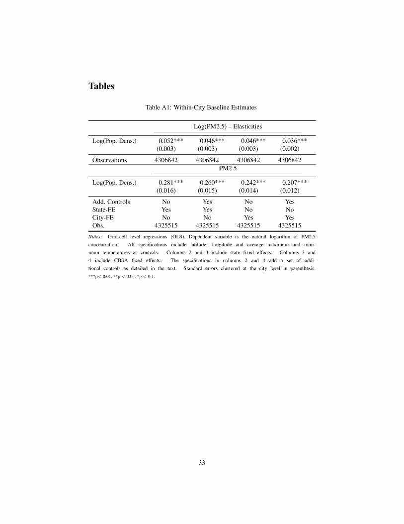
Table A1: Within-City Baseline Estimates

Log(PM2.5) – Elasticities

Log(Pop. Dens.) 0.052*** 0.046*** 0.046*** 0.036***(0.003) (0.003) (0.003) (0.002)

Observations 4306842 4306842 4306842 4306842PM2.5

Log(Pop. Dens.) 0.281*** 0.260*** 0.242*** 0.207***(0.016) (0.015) (0.014) (0.012)

Add. Controls No Yes No YesState-FE Yes Yes No NoCity-FE No No Yes YesObs. 4325515 4325515 4325515 4325515

Notes: Grid-cell level regressions (OLS). Dependent variable is the natural logarithm of PM2.5concentration. All specifications include latitude, longitude and average maximum and mini-mum temperatures as controls. Columns 2 and 3 include state fixed effects. Columns 3 and4 include CBSA fixed effects. The specifications in columns 2 and 4 add a set of addi-tional controls as detailed in the text. Standard errors clustered at the city level in parenthesis.***p< 0.01, **p < 0.05, *p < 0.1.

33

Table A2: Within-City First-Stage Coefficients

Log-Density

Soil Drainage -0.097*** -0.175*** -0.024 -0.072***(0.034) (0.030) (0.022) (0.021)

Earthquake Risk 0.420*** 0.526*** 0.297** 0.341**(0.083) (0.088) (0.133) (0.140)

Aquifer 0.310*** 0.041 0.656*** 0.341***(0.109) (0.105) (0.109) (0.097)

Add. Controls No No No YesState-FE Yes Yes No NoCity-FE No No Yes YesF-Stat 12 25 15 10Obs. 4325515 4325515 4325515 4325515

Notes: Grid-cell level regressions (OLS). Dependent variable is the natural logarithm of PM2.5concentration. All specifications include latitude, longitude and average maximum and mini-mum temperatures as controls. Columns 2 and 3 include state fixed effects. Columns 3 and4 include CBSA fixed effects. The specifications in columns 2 and 4 add a set of addi-tional controls as detailed in the text. Standard errors clustered at the city level in parenthesis.***p< 0.01, **p < 0.05, *p < 0.1.

Table A3: First-Stage (Geological Instruments) - City Level

Log(Density)

Earthquake Risk 0.210*** 0.289*** 0.258***(0.057) (0.080) (0.074)

Aquifer -0.220** -0.154 -0.155(0.091) (0.109) (0.102)

Soil Drainage -0.187*** -0.309*** -0.333***(0.040) (0.049) (0.052)

Add. Controls No No YesState-FE No Yes YesF-Stat 21 24 20Obs. 933 933 933

Notes: City-level regressions. The dependent variable in all columns is the log of population densityat the city (CBSA) level. F-statistics for joint significance of the geological instruments reported in thetable foot. All specifications include latitude, longitude and average maximum and minimum tempera-tures as controls. The specifications in columns 2 and 3 add state effects. The specifications in col-umn 3 add a set of additional controls as detailed in the text. Robust standard errors in parentheses.***p< 0.01, **p < 0.05, *p < 0.1.

34

Table A4: Balancing - Power Stations

N. Oil Plants N. Coal Plants Dummy Oil Dummy Coal

Soil Drainage -0.009 0.262 -0.008 0.029*(0.064) (0.183) (0.017) (0.016)

Earthq. Risk 0.008 -0.040 0.002 -0.041(0.046) (0.503) (0.026) (0.029)

Aquifer 0.034 0.304 0.033 -0.031(0.103) (0.275) (0.039) (0.040)

Add. Controls Yes Yes Yes YesState-FE Yes Yes Yes YesF-Stat 0 2 0 2Obs. 933 933 933 933

Notes: City-level regressions of instruments on variables measuring the presence ofoil and coal power stations. All specifications include the full set of controls and stateeffects. The dependent variables are the number of stations of each type in columns1 and 2, and dummies taking value 1 if any station is present on columns 3 and 4.F-statistics for joint significance of the geological instruments included in table footer.

Table A5: Balancing - Wharton Index

LUR Index LUR Index LUR Index LUR Index

Soil Drainage -0.134** -0.053 -0.025 -0.073(0.053) (0.058) (0.050) (0.055)

Earthquake Risk 0.223*** -0.027 0.169* 0.178*(0.070) (0.073) (0.092) (0.093)

Aquifer 0.587*** -0.013 0.176 0.090(0.126) (0.116) (0.118) (0.128)

Add. Controls No Yes No YesState-FE No No Yes YesF-Stat 9 0 2 2Obs. 485 485 485 485

Notes: City-level regressions of instruments on Wharton Land Use Regulation Index (Gyourko et al. 2008).All specifications include latitude, longitude and average maximum and minimum temperatures as controls.Columns 2 and 5 include additional controls as outlined in the text. Columns 3 and 4 include state effects.F-statistics for joint significance of the geological instruments included in table footer.

35

Table A6: Robustness: Instrument Pairs

Log(PM2.5)

Log(Pop. Dens.) 0.094** 0.160*** 0.126***(0.038) (0.022) (0.023)

Log(Pop. Dens.) 0.303*** 0.216*** 0.195***(0.048) (0.040) (0.039)

Log(Pop. Dens.) 0.100*** 0.150*** 0.113***(0.038) (0.019) (0.022)

Add.Controls No No YesState-FE No Yes YesObs. 933 933 933

Notes: 2SLS Estimates in each row obtained by excluding one of the geological variables when instrument-ing for density: First row excludes earthquake risk, the second excludes soil drainage capacity, and the thirdaquifer presence. Dependent variable is the log of population-weighted PM2.5 concentration. All specifica-tions include latitude, longitude and average maximum and minimum temperatures as controls. State effectsadded in columns 2 and 3. The specifications in column 3 add additional controls, as detailed in the text.Robust standard errors in parentheses. ***p< 0.01, **p < 0.05, *p < 0.1

Table A7: Robustness: Commuting Zones (IV Estimates)

Log(PM2.5) - Elasticities

Log(Pop. Dens.) 0.209*** 0.133*** 0.110***(0.030) (0.022) (0.023)

Observations 524 522 522PM2.5 (Exposure)

Log(Pop. Dens.) 1.573*** 0.979*** 0.866***(0.215) (0.154) (0.156)

Add. Controls Yes Yes YesState-FE No Yes YesF-Stat 21 13 16Obs. 524 522 522

Notes: Sample of 2010 commuting zones, obtained from Fowler et al. (2016). 2SLS estimates obtainedusing our geological instruments. For the first row of estimates, the dependent variable is the natural log-arithm of PM2.5 exposure as defined in the text. The dependent variable for the second row of estimatesis this variable in levels. All specifications include latitude, longitude and average maximum and minimumtemperatures as controls. The specifications in columns 2 and 3 add state effects. The specifications incolumn 3 add a set of additional controls as detailed in the text. F-statistics for joint significance of thegeological instruments in the first-stage, reported in the table foot. Robust standard errors in parentheses.***p< 0.01, **p < 0.05, *p < 0.1

36

Table A8: Robustness: MSAs - IV Elasticity Estimates

Log(PM2.5) - Elasticities

Log(Pop. Dens.) 0.367*** 0.215*** 0.206***(0.063) (0.041) (0.047)

Controls No No YesState-FE No Yes YesF-stat 15 13 12Obs. 361 361 361

Notes: Sample restricted to Metropolitan Areas (MSAs). Instrumental variable 2SLS estimates obtained us-ing our geological instruments (earthquake risk and soil drainage) and log population density from the 1880census. The unit of analysis is the city (CBSA). The dependent variable is the natural logarithm of residen-tial average PM2.5 exposure in all specifications. All specifications include latitude, longitude and averagemaximum and minimum temperatures as controls. The specifications in column 2 add state effects. The spec-ifications in column 3 add a set of additional controls, as detailed in the text. F-statistics for joint significanceof the three instruments in the first-stage, reported in the table foot. Robust standard errors in parentheses.***p< 0.01, **p < 0.05, *p < 0.1

37

38

References

Ahlfeldt, G. M., & Pietrostefani, E. (2019). The economic effects of density: A synthesis. Journal of

Urban Economics, 111, 93-107.

Bertaud, A., & Malpezzi, S. (2003). The spatial distribution of population in 48 world cities:

Implications for economies in transition. Center for urban land economics research, University of

Wisconsin, 22.

Bondy, M., Roth, S., & Sager, S. (2018). Crime Is In The Air: The Contemporaneous Relationship

between Air Pollution and Crime. LSE mimeo

Borck, R. (2016). Will skyscrapers save the planet? Building height limits and urban greenhouse gas

emissions. Regional Science and Urban Economics, 58, 13-25.

Borck, R., & Schrauth, P. (2019). Population density and urban air quality.

Burchfield, M., Overman, H. G., Puga, D., & Turner, M. A. (2006). Causes of sprawl: A portrait from

space. The Quarterly Journal of Economics, 121(2), 587-633.

Carleton, T., Delgado, M., Greenstone, M., Houser, T., Hsiang, S., Hultgren, A., ... & Rising, J. (2018).

Valuing the Global Mortality Consequences of Climate Change Accounting for Adaptation Costs and

Benefits.

Chay, K. Y., & Greenstone, M. (2003). The impact of air pollution on infant mortality: evidence from

geographic variation in pollution shocks induced by a recession. The Quarterly Journal of

Economics, 118(3), 1121-1167.

Ciccone, A., & Hall, R. E. (1996). Productivity and the density of economic activity. The American

Economic Review, 86(1), 54.

Combes, P. P., Duranton, G., & Gobillon, L. (2008). Spatial wage disparities: Sorting matters! Journal

of Urban Economics, 63(2), 723-742.

Combes, P. P., Duranton, G., Gobillon, L., & Roux, S. (2010). Estimating Agglomeration Economies

with History, Geology, and Worker Effects. Agglomeration Economics, 15.

Combes, P. P., & Gobillon, L. (2015). The empirics of agglomeration economies. In Handbook of

regional and urban economics (Vol. 5, pp. 247-348). Elsevier.

Dockery, D. W., Pope, C. A., Xu, X., Spengler, J. D., Ware, J. H., Fay, M. E., ... & Speizer, F. E.

(1993). An association between air pollution and mortality in six US cities. New England journal of

medicine, 329(24), 1753-1759.

Duranton, G., & Turner, M. A. (2018). Urban form and driving: Evidence from US cities. Journal of

Urban Economics, 108, 170-191.

Ebenstein, A., Lavy, V., & Roth, S. (2016). The long-run economic consequences of high-stakes

examinations: evidence from transitory variation in pollution. American Economic Journal: Applied

Economics, 8(4), 36-65.

Fowler, Christopher S., Danielle C. Rhubart, and Leif Jensen. "Reassessing and revising commuting

zones for 2010: History, assessment, and updates for US ‘labor-sheds’ 1990–2010." Population

Research and Policy Review 35.2 (2016): 263-286.

Fowlie, M., Rubin, E. A., & Walker, R. (2019). Bringing Satellite-Based Air Quality Estimates Down

to Earth (No. w25560). National Bureau of Economic Research.

39

Fragkias, M., Lobo, J., Strumsky, D., & Seto, K. C. (2013). Does size matter? Scaling of CO2

emissions and US urban areas. PLoS One, 8(6), e64727.

Gaigné, Carl, Stéphane Riou, and Jacques-François Thisse. 2012. Are compact cities environmentally

friendly? Journal of Urban Economics, 72(2-3): 123–136

Glaeser, E. L., & Kahn, M. E. (2010). The greenness of cities: carbon dioxide emissions and urban

development. Journal of Urban Economics, 67(3), 404-418.

Graff Zivin, J., & Neidell, M. (2012). The impact of pollution on worker productivity. American

Economic Review, 102(7), 3652-73.

Gyourko, J., Saiz, A., & Summers, A. (2008). A new measure of the local regulatory environment for

housing markets: The Wharton Residential Land Use Regulatory Index. Urban Studies, 45(3), 693-

729.

Hettige, H., Martin, P., Singh, M., & Wheeler, D. (1995). The industrial pollution projection

system. World Bank policy research working paper, (1431).

Hilber, Christian, and Charles Palmer (2014). Urban development and air pollution: Evidence from a

global panel of cities. Mimeo

Holian, M. J., & Kahn, M. E. (2015). Household demand for low carbon policies: Evidence from

California. Journal of the Association of Environmental and Resource Economists, 2(2), 205-234.

Kahn, M. E., & Walsh, R. (2015). Cities and the Environment. In Handbook of regional and urban

economics (Vol. 5, pp. 405-465). Elsevier.

Lee, S., & Lee, B. (2014). The influence of urban form on GHG emissions in the US household

sector. Energy Policy, 68, 534-549.

McDonald, John F. "Econometric studies of urban population density: a survey." Journal of urban

economics 26 (1989): 361-85.

Norman, J., MacLean, H. L., & Kennedy, C. A. (2006). Comparing high and low residential density:

life-cycle analysis of energy use and greenhouse gas emissions. Journal of urban planning and

development, 132(1), 10-21.

OECD (2014). The Cost of Air Pollution. Health Impacts and Road Transport.

Pope 3rd, C. A., Bates, D. V., & Raizenne, M. E. (1995). Health effects of particulate air pollution:

time for reassessment?. Environmental health perspectives, 103(5), 472.

Rosenthal, Stuart S, and William C Strange. 2008. “The attenuation of human capital spillovers.”

Journal of Urban Economics, 64(2): 373–389.

Schlenker, W., & Walker, W. R. (2015). Airports, air pollution, and contemporaneous health. The

Review of Economic Studies, 83(2), 768-809.

Sarzynski, Andrea. (2012). “Bigger is not always better: a comparative analysis of cities and their air

pollution impact.” Urban Studies, 49(14): 3121–3138

Stevens, M. R. (2017). Does compact development make people drive less? Journal of the American

Planning Association, 83(1), 7-18.

United Nations (2015). World urbanization prospects: The 2014 revision. United Nations Department

of Economics and Social Affairs, Population Division: New York, NY, USA. #

US Environmental Protection Agency. (2012). Regulatory Impact Analysis for the Final Revisions to

the National Ambient Air Quality Standards for Particulate Matter.

40

Van Donkelaar, A., R. V. Martin, R. J. D. Spurr and R. T. Burnett (2015). High-resolution satellite-

derived PM2.5 from optimal estimation and geographically weighted regression over North America,

Environ. Sci. and Tech..

VandeWeghe, J. R., & Kennedy, C. (2007). A spatial analysis of residential greenhouse gas emissions

in the Toronto census metropolitan area. Journal of industrial ecology, 11(2), 133-144.

World Bank; Institute for Health Metrics and Evaluation. (2016). The Cost of Air Pollution:

Strengthening the Economic Case for Action. World Bank, Washington, DC. © World Bank

World Health Organization (2019). Air pollution and Health: Summary. Retrieved from

http://www.who.int/airpollution/ambient/about/en/

CENTRE FOR ECONOMIC PERFORMANCE

Recent Discussion Papers

1634 Nicholas Bloom

John Van Reenen

Heidi Williams

A Toolkit of Policies to Promote Innovation

1633 Stephan E. Maurer

Ferdinand Rauch

Economic Geography Aspects of the Panama

Canal

1632 Nikhil Datta Willing to Pay for Security: A Discrete

Choice Experiment to Analyse Labour Supply

Preferences

1631 Gabriel M. Ahlfeldt

Volker Nitsch

Nicolai Wendland

Ease Versus Noise: Long-Run Changes in the

Value of Transport (Dis)amenities

1630 Grace Lordan

Alistair McGuire

Widening the High School Curriculum to

Include Soft Skill Training: Impacts on

Health, Behaviour, Emotional Wellbeing and

Occupational Aspirations

1629 Per-Anders Edin

Tiernan Evans

Georg Graetz

Sofia Hernnäs

Guy Michaels

Individual Consequences of Occupational

Decline

1628 Pawel Bukowski

Filip Novokmet

Between Communism and Capitalism: Long-

Term Inequality in Poland, 1892-2015

1627 Thomas Sampson Technology Gaps, Trade and Income

1626 Andrea Ichino

Martin Olsson

Barbara Petrongolo

Peter Skogman Thoursie

Economic Incentives, Home Production and

Gender Identity Norms

1625 Richard Murphy Why Unions Survive: Understanding How

Unions Overcome the Free-Rider Problem

1624 Natalie Chen

Wanyu Chung

Dennis Novy

Vehicle Currency Pricing and Exchange Rate

Pass-Through

1623 Michael Amior

Alan Manning

Commuting, Migration and Local Joblessness

1622 Rui Costa

Swati Dhingra

Stephen Machin

Trade and Worker Deskilling

1621 Jan-Emmanuel De Neve

Clement Imbert

Johannes Spinnewijn

Teodora Tsankova,

Maarten Luts

How to Improve Tax Compliance? Evidence

from Population-wide Experiments in

Belgium

1620 David S. Jacks

Dennis Novy

Trade Blocs and Trade Wars during the

Interwar Period

1619 Giulia Faggio

Olmo Silva

William C. Strange

Tales of the City: What Do Agglomeration

Cases Tell Us About Agglomeration in

General?

1618 Andrew Mountford

Jonathan Wadsworth

Trainspotting: ‘Good Jobs’, Training and

Skilled Immigration

1617 Marta De Philippis

Federico Rossi

Parents, Schools and Human Capital

Differences across Countries

1616 Michael Amior Education and Geographical Mobility: The

Role of Wage Rents

The Centre for Economic Performance Publications Unit

Tel: +44 (0)20 7955 7673 Email info@cep.lse.ac.uk

Website: http://cep.lse.ac.uk Twitter: @CEP_LSE