and physics inﬂuence of future ... - atmos-chem-phys.net · atmos. chem. phys., 14, 1011–1024,...

Atmos. Chem. Phys., 14, 1011–1024, 2014www.atmos-chem-phys.net/14/1011/2014/doi:10.5194/acp-14-1011-2014© Author(s) 2014. CC Attribution 3.0 License.

Atmospheric Chemistry

and PhysicsO

pen Access

Influence of future climate and cropland expansion on isopreneemissions and tropospheric ozone

O. J. Squire1, A. T. Archibald 1,2, N. L. Abraham1,2, D. J. Beerling3, C. N. Hewitt4, J. Lathière3,4,*, R. C. Pike1,** ,P. J. Telford1,2, and J. A. Pyle1,2

1Centre for Atmospheric Science, Department of Chemistry, University of Cambridge, Cambridge, CB2 1EW, UK2National Centre for Atmospheric Science, Department of Chemistry, University of Cambridge, Cambridge, CB2 1EW, UK3Department of Animal and Plant Sciences, University of Sheffield, Sheffield, S10 2TN, UK4Lancaster Environment Centre, Lancaster University, Lancaster, LA1 4YQ, UK* now at: Laboratoire des Sciences du Climat et de l’Environnement, IPSL, UVSQ, CEA, CNRS, Gif-sur-Yvette, France** now at: Draper Fisher Jurvetson, 2882 Sand Hill Road, Suite 150 Menlo Park, CA 94025, USA

Correspondence to:O. J. Squire ([email protected])

Received: 29 May 2013 – Published in Atmos. Chem. Phys. Discuss.: 9 July 2013Revised: 19 December 2013 – Accepted: 19 December 2013 – Published: 28 January 2014

Abstract. Over the 21st century, changes in CO2 levels, cli-mate and land use are expected to alter the global distributionof vegetation, leading to changes in trace gas emissions fromplants, including, importantly, the emissions of isoprene.This, combined with changes in anthropogenic emissions,has the potential to impact tropospheric ozone levels, whichabove a certain level are harmful to animals and vegetation.In this study we use a biogenic emissions model followingthe empirical parameterisation of the MEGAN model, withvegetation distributions calculated by the Sheffield DynamicGlobal Vegetation Model (SDGVM) to explore a range ofpotential future (2095) changes in isoprene emissions causedby changes in climate (including natural land use changes),land use, and the inhibition of isoprene emissions by CO2.From the present-day (2000) value of 467 Tg C yr−1, we findthat the combined impact of these factors could cause a netdecrease in isoprene emissions of 259 Tg C yr−1 (55 %) withindividual contributions of +78 Tg C yr−1 (climate change),−190 Tg C yr−1 (land use) and−147 Tg C yr−1 (CO2 inhibi-tion). Using these isoprene emissions and changes in anthro-pogenic emissions, a series of integrations is conducted withthe UM-UKCA chemistry-climate model with the aim of ex-amining changes in ozone over the 21st century. Globally, allcombined future changes cause a decrease in the troposphericozone burden of 27 Tg (7 %) from 379 Tg in the present-day.At the surface, decreases in ozone of 6–10 ppb are calcu-lated over the oceans and developed northern hemisphericregions, due to reduced NOx transport by PAN and reduc-

tions in NOx emissions in these areas respectively. Increasesof 4–6 ppb are calculated in the continental tropics due tocropland expansion in these regions, increased CO2 inhibi-tion of isoprene emissions, and higher temperatures due toclimate change. These effects outweigh the decreases in trop-ical ozone caused by increased tropical isoprene emissionswith climate change. Our land use change scenario consistsof cropland expansion, which is most pronounced in the trop-ics. The tropics are also where land use change causes thegreatest increases in ozone. As such there is potential for in-creased crop exposure to harmful levels of ozone. However,we find that these ozone increases are still not large enoughto raise ozone to such damaging levels.

1 Introduction

Plants emit biogenic volatile organic compounds (BVOCs)into the Earth’s atmosphere, with the largest fluxes being forisoprene (2-methyl-1,3-butadiene), with annual emissions of∼ 500 TgC (Guenther et al., 2006). This value is greaterthan the total amount of non-methane hydrocarbons releasedannually due to anthropogenic activities. However, not allplants emit isoprene, and those that do, emit it in very differ-ent amounts. For example, broad-leaved rainforest has beenmeasured to emit∼ 2.5 mgm−2h−1 (Rinne et al., 2002; Mis-ztal et al., 2011), whilst crops such as maize and sugarcaneare thought to emit much less isoprene (∼ 0.09 mgm−2h−1,

Published by Copernicus Publications on behalf of the European Geosciences Union.

1012 O. J. Squire et al.: Influence of future cropland expansion on tropospheric ozone

Guenther et al., 2006). On the other hand, much greater iso-prene fluxes of up to 13.0 mgm−2h−1 have been measuredfrom fast-growing plants such as oil palm (Misztal et al.,2011). Isoprene is a very reactive VOC that is readily ox-idised in the atmosphere, and in the presence of oxides ofnitrogen (NOx = NO+ NO2), it can lead to the formationof ozone (O3) (e.g. Chameides et al., 1988). However thechemical relationship between VOCs, NOx and O3 is non-linear; the response of O3 to changes in either precursor gasdepends on their ratio (see the Empirical Kinetics ModelingApproach diagrams in, e.g.Dodge, 1977; Sillman and He,2002). In sufficient quantities, O3 is recognised to be damag-ing to both humans and plants (WHO, 2000), and has beenshown to lead to substantial losses in global crop yields (Avn-ery et al., 2011a). As isoprene is a precursor to O3 formation,changes to factors that influence isoprene emissions have thepotential to alter the degree of O3 damage to the biosphere.

There are several factors that can affect isoprene emis-sions. From a fixed vegetation distribution, isoprene emis-sions are directly stimulated by increases in temperature fol-lowing an Arrhenius-like relationship (Tingey et al., 1979),and are directly inhibited under elevated concentrations ofCO2 (Rosenstiel et al., 2003). However, increased CO2 lev-els may also lead indirectly to greater isoprene emissionsby extended fertilisation of the biosphere (e.g. Tao and Jain,2005; Arneth et al., 2007). Similarly, increases in tempera-ture may indirectly decrease isoprene emissions by decreas-ing soil moisture, thus leading to “die-back” of isoprene-emitting vegetation (Cox et al., 2000, 2004; Sanderson et al.,2003). Changes in land use that affect the extent and distri-bution of vegetation also have the potential to alter isopreneemissions. Anthropogenic land use change, on the globalscale, contributes a net decrease to isoprene emissions asgenerally this involves replacement of high isoprene emit-ters with lower ones (e.g. Tao and Jain, 2005; Lathière et al.,2005; Wu et al., 2012). However, this is not always the case,especially on the regional scale where some land use sce-narios show increased isoprene emissions. Examples are thereplacement of broad-leaved rainforest with oil palm (Hewittet al., 2009; Ashworth et al., 2012; Warwick et al., 2013)or agricultural cropland withArundo donaxfor biofuel pro-duction (Porter et al., 2012). In the current study we do notinclude such land use changes.

There is a fine balance between those factors that increaseisoprene emissions (direct effects of temperature, CO2 fertil-isation), and those that decrease them (die-back, CO2 inhi-bition, land use change). This balance may well change overthe next century. Rising CO2 levels are expected to causerises in temperature and CO2 fertilisation, which would leadto isoprene emission increases. Some studies calculate thatthese increases would be more than compensated for by in-creases in CO2 inhibition (Heald et al., 2009; Young et al.,2009; Pacifico et al., 2012) and anthropogenic land usechange (Ganzeveld et al., 2010; Wu et al., 2012). Howeverthe magnitude of these terms and the degree to which they

compensate each other is scenario dependent and still re-mains highly uncertain.

Due to the non-linearity of VOC-NOx-O3 chemistry, theO3 response to these isoprene emission changes dependson whether the environment is NOx-limited or VOC-limited(Wiedinmyer et al., 2006; Zeng et al., 2008; Young et al.,2009; Wu et al., 2012; Pacifico et al., 2012). When sufficientNOx is available, isoprene reacts with OH and molecularoxygen to produce hydroxyperoxy radicals, which convertNO to NO2, leading to O3 formation. In low NOx, VOC-rich environments, the rate of this NOx-dependent pathwaydecreases, and it becomes more favourable for isoprene tobe oxidised directly by O3, leading to O3 removal. O3 pro-duction is further limited by the removal of NOx as isoprenehydroxyperoxy radicals react with NO to form isoprene ni-trates. The degree to which NOx is regenerated from isoprenenitrate degradation remains uncertain (Fiore et al., 2012), andhas a significant effect on the O3 response to isoprene emis-sion changes (von Kuhlmann et al., 2004; Wu et al., 2007;Horowitz et al., 2007).

The first aim of this current study is to explore how con-tributions from the main factors that affect tropospheric O3could change over the 21st century. This is achieved by useof a global chemistry-climate model (the UK MetOffice Uni-fied Model coupled to the UK Chemistry and Aerosol model(UM-UKCA)) as detailed in Sect.2. One of the factors in-vestigated is changes in isoprene emissions, and in this sec-tion we also outline the method used for calculating theseisoprene emission changes. In Sect. 3 the generated isopreneemissions are analysed to show how they could change overthe 21st century due to changes in climate, land use and CO2inhibition. In Sect.4 we use the results of the UM-UKCAintegrations to attribute future O3 changes to changes in cli-mate, isoprene emissions with climate, anthropogenic emis-sions, land use and CO2 inhibition of isoprene emissions.

The second aim of this study is to determine whetherchanges in isoprene emissions due to anthropogenic landuse (simulated here as cropland expansion) could cause in-creased exposure of those crops to harmful levels of O3.This is addressed in Sect.5 by calculating the effect of crop-land expansion on the “Accumulated exposure (to O3) Overa Threshold of 40 ppb” (AOT40) diagnostic. The AOT40is recommended by the World Health Organization (WHO,2000) as a diagnostic for quantifying harmful O3 exposureto vegetation. The effects of changes in O3 on crop damagehave been examined in several previous studies (e.g.Ash-more, 2005; Van Dingenen et al., 2009; Fuhrer, 2009; Avneryet al., 2011b), however very few studies consider specificallythe contribution from isoprene emission changes (Ashworthet al., 2012, 2013), which is the focus here.

Isoprene oxidation chemistry is too complex to include ex-plicitly in a global model, so the chemistry must be parame-terised. This introduces uncertainties, which we investigatein a companion paper (Squire et al., 2014) by comparingfour different isoprene chemical schemes, all of which are

Atmos. Chem. Phys., 14, 1011–1024, 2014 www.atmos-chem-phys.net/14/1011/2014/

O. J. Squire et al.: Influence of future cropland expansion on tropospheric ozone 1013

currently used in Earth System Models. One notable sourceof uncertainty is the degree to which HOx is regeneratedfrom isoprene degradation under low NOx conditions. Re-cent studies have demonstrated biases between measured andmodelled HO2 (Fuchs et al., 2011) and OH (Mao et al., 2012)under high VOC (low NOx) conditions. Proposals have beenput forward for missing mechanistic pathways (e.g.Paulotet al., 2009; Peeters et al., 2009) that to some extent recon-cile these discrepancies (Archibald et al., 2010). In the com-panion paper we investigate the sensitivity of our results toincluding these new pathways.

2 Model and Experiment

In order to establish how contributions from the main fac-tors that affect tropospheric O3 could change over the 21stcentury, a present-day (2000) integration and a range of fu-ture (2095) integrations were conducted with UM-UKCA asdetailed in Sect.2.3. For all integrations isoprene emissionswere first calculated offline using a dynamic global vegeta-tion model and a biogenic emissions model as described inSect. 2.1. Additionally, to investigate the effect of changes inland use the distribution of land surface types in UM-UKCAhad to be altered, and this process is described in Sect. 2.2.

2.1 Isoprene emission calculations

Isoprene emissions were calculated under present-day (2000)conditions and for a series of future (2095) conditions. InSect.3 differences in these emissions are analysed to as-certain individual contributions to future isoprene emissionchanges from future changes in climate, land use, CO2 inhi-bition of isoprene emissions and the combined effect of all ofthese factors. In all cases first the vegetation distribution wasdetermined using the Sheffield Dynamic Global VegetationModel (SDGVM) (Beerling et al., 1997; Beerling and Wood-ward, 2001). The model was run in time slices, for present-day (2000) and future (2095) conditions, each time being runto vegetative equilibrium. The SDGVM calculates the po-tential distribution and leaf area index of six plant functionaltypes (PFTs): C3 and C4 grasses, evergreen broad-leaved andneedle-leaved trees, and deciduous broad-leaved and needle-leaved trees (Lathière et al., 2010). The SDGVM was drivenby climate conditions generated with the HadGEM1 model(Johns et al., 1997). For calculation of the future isopreneemissions the SRES B2 climate scenario was used (Riahiet al., 2007). The vegetation distribution from the SDGVMwas then used as input for a biogenic emissions model basedon MEGAN (Guenther et al., 2006), as described inLathièreet al.(2010), which produced the isoprene emissions. Addi-tionally, when future CO2 inhibition of isoprene emissionswas included, the parameterisation ofPossell et al.(2005)was used in the biogenic emissions model, as inLathièreet al.(2010).

Discussion

Paper

|D

iscussionP

aper|

Discussion

Paper

|D

iscussionP

aper|

Discu

ssionPaper

|Discu

ssionPaper

|Discu

ssionPaper

|Discu

ssionPaper

|

Latit

ude

Longitude

−180° −90° 0° 90° 180°

−40°

−20°

0°

20°

40°

60°(a) C3 grasses (b) Broad−leaved trees

−40°

−20°

0°

20°

40°

60°(c) Bare soil

−180° −90° 0° 90° 180°

(d) Other

−1.0 −0.8 −0.6 −0.4 −0.2 0.0 0.2 0.4 0.6 0.8 1.0

Fig. 2. Change in gridcell fraction of UM-UKCA land surface types between present day (2000)and the land use scenario for 2095 (2095 - 2000). Changes in the crop fraction (assigned to C3grasses) were calculated using the IMAGE 2.1 model (Alcamo, 1999).

31

Fig. 1. Change in gridcell fraction of UM-UKCA land surface types between present day (2000)and the anthropogenic land use scenario (cropland expansion) for 2095 (2095–2000). Changesin the crop fraction (assigned to C3 grasses) were calculated using the IMAGE 2.1 model (Al-camo, 1999).

34

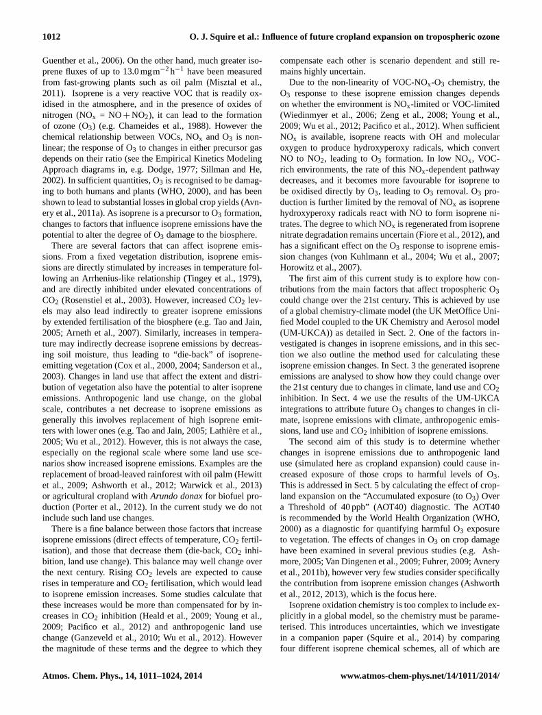
Fig. 1.Change in grid cell fraction of UM-UKCA land surface typesbetween present-day (2000) and the anthropogenic land use sce-nario (cropland expansion) for 2095 (2095–2000). Changes in thecrop fraction (assigned to C3 grasses) were calculated using the IM-AGE 2.1 model (Alcamo, 1999).

2.2 Land surface changes

As the SDGVM does not explicitly calculate the distribu-tion of crops, for the inclusion of future cropland expansionthe IMAGE 2.1 model (Alcamo, 1999) was used to generatea crop map in line with the A1B SRES scenario (Nakicen-ovic et al., 2000). This crop map was then combined withthe natural vegetation distribution from the SDGVM to cre-ate a new distribution of PFTs and leaf area index, and thiswas used as input for the biogenic emissions model that gavethe altered isoprene emissions. The new PFT distribution andleaf area index was also used in those UM-UKCA integra-tions that included future cropland expansion, as the PFT af-fects a number of model surface properties such as the chemi-cal deposition velocity and surface roughness. In UM-UKCAthere are nine land surface types (LSTs): broad-leaved trees,needle-leaved trees, C3 grasses, C4 grasses, shrubs, baresoil, urban, ice and inland water. These LSTs do not corre-spond exactly to the PFTs calculated by the SDGVM, and assuch in the land use change integrations the SDGVM PFTshad to be mapped onto the UM-UKCA LSTs. As C3 andC4 grasses exist in both models their distributions in UM-UKCA followed that of the SDGVM, with the addition thatall crops were also assigned to C3 grasses. This simplificationcould be made as in UM-UKCA the deposition properties ofboth grass types are identical and there are only small dif-ferences in other surface properties including aerodynamicresistance. Both broad-leaved and needle-leaved categoriesin the SDGVM were mapped to broad-leaved and needle-leaved trees respectively in UM-UKCA. Figure1 shows thedifference in the grid cell fraction of UM-UKCA LSTs be-tween 2000 and 2095 for the land use change scenario. The

www.atmos-chem-phys.net/14/1011/2014/ Atmos. Chem. Phys., 14, 1011–1024, 2014


Table 1. Model integrations conducted with UM-UKCA (BASE and Runs 1–6). PD = present-day (2000), Fut = Future (2095). The lowersection of the table indicates how changes due to each perturbation are calculated.

UM-UKCA Climate Isoprene Anthrop- Land use CO2integration emissions ogenic inhibition

with climate emissions

BASE PD PD PD PD PDRun1 Fut PD PD PD PDRun2 Fut Fut PD PD PDRun3 Fut Fut Fut PD PDRun4 Fut Fut Fut Fut PDRun5 Fut Fut Fut PD FutRun6 Fut Fut Fut Fut Fut

1 Climate 1 Isoprene 1 Anthrop- 1 Land use 1 CO2 1 Allemissions ogenic inhibition factors

with climate emissions

Run1 – BASE Run2 – Run1 Run3 – Run2 Run4 – Run3 Run5 – Run3 Run6 – Run1

IMAGE model calculated an increase in croplands by 2095of 6.34×1012m2 (135 %), which corresponds to an increasein the fraction of C3 grasses in UM-UKCA as shown inFig. 1a. This expansion of crops was largely at the expenseof broad-leaved trees, which show large decreases (Fig.1b).As broad-leaved trees have a higher isoprene emission fac-tor than crops, 12.6 and 0.09 mg isoprene m−2h−1 respec-tively (Guenther et al., 2006; Lathière et al., 2010), croplandexpansion resulted in a decrease in isoprene emissions. Thefraction of needle-leaved trees and C4 grasses also decreased(lumped into “Other”; Fig.1d), as did those LSTs not in-cluded in the SDGVM. These LSTs were adapted from theirpresent-day UM-UKCA values to account for cropland ex-pansion such that in a grid cell where crops increased bya given percentagex, each LST was decreased byx %.

2.3 Chemistry-climate integrations

Table 1 summarises the integrations conducted with UM-UKCA. The configuration of UM-UKCA used for all inte-grations was the Hadley Centre Global Environment Modelversion 3 – Atmosphere only (HadGEM3-A r2.0) at UM ver-sion 7.3, which includes UKCA (O’Connor et al., 2013).UM-UKCA was run at a horizontal resolution of 3.75◦ lon-gitude× 2.5◦ latitude on 60 hybrid height levels that stretchfrom the surface to∼ 84 km. The model setup is similar tothat described inTelford et al.(2010), with the Chemistry ofthe Troposphere (CheT) chemical mechanism that consistsof 56 chemical tracers, 165 photochemical reactions, dry de-position of 32 species and wet deposition of 23 species. Iso-prene chemistry in CheT follows that of the Mainz IsopreneMechanism (MIM) (Pöschl et al., 2000). The Fast-JX pho-tolysis scheme (Neu et al., 2007) is used as implementedin Telford et al.(2013). This tropospheric version of UM-UKCA employs a simplified stratospheric chemistry and, to

provide a realistic upper boundary condition for the tracers,concentrations of O3 and NOy are overwritten above 30 hPafrom zonal mean values from the Cambridge 2-D model(Law and Pyle, 1993a,b) as inTelford et al.(2010). All inte-grations lasted five model years plus a “spin-up” period of 16months. The present-day integration (BASE) was a year 2000time slice and the future integrations were 2095 time slices,in which perpetual 2000 (BASE) and 2095 (future) sea sur-face temperatures (SSTs), sea ice concentrations (SICs) andgreenhouse gases (GHGs) were used. Minimising year-to-year variability in this way ensured that differences betweenmodel integrations would be due only to the deliberate per-turbation that was made (e.g. changing isoprene emissions).

In the BASE integration, mixing ratios of GHGs were370 ppm (CO2) and 1765 ppb (CH4). SSTs and SICs weretaken from a 1998–2002 climatology following the HadISSTdata set (Rayner et al., 2003). For those integrations witha 2095 climate (see Table1), GHGs were changed to621 ppm (CO2) and 2975 ppb (CH4) following the SRES B2scenario (Riahi et al., 2007), and SSTs and SICs were takenfrom integrations generated by the HadGEM1 model (Stottet al., 2006) in line with the A1B SRES scenario (Nakicen-ovic et al., 2000).

In the present-day, anthropogenic emissions of NOx, car-bon monoxide, formaldehyde, ethane, propane, acetone andacetaldehyde were taken from the Edgar3.2 data set (Olivierand Berdowski, 2001). In those 2095 integrations with fu-ture anthropogenic emissions, these emissions followed theB2+ CLE scenario (Fowler et al., 2008). This scenario isan updated version of the IPCC B2 scenario (Riahi et al.,2007) to account for Current LEgislation passed in 2002 to2006 (Dentener et al., 2005). This scenario has only smallincreases in emissions from emerging economies, and largeemission reductions across developed countries (USA, Eu-rope, Japan).



We acknowledge that more than one future scenario hasbeen followed in our experiments. However, our aim is notto produce a realistic “prediction” of future conditions, ratherto investigate how O3 responds to changes in a range of pa-rameters. As such, our aim is to explain the sensitivity ofO3, and O3 feedbacks, to plausible future changes in natu-ral and anthropogenic forcing mechanisms. The climate sce-nario (essentially B2) gives a climate change signal in themid-range of the SRES scenarios. As such, we expect thisto result in a moderate O3 signal. For land use change, theprimary variable of interest to this work, the A1B scenariowas used, which is characterised by extensive cropland ex-pansion. The aim was to calculate a clear signal in the O3response from land use change that involved a large changein isoprene emissions. This was paired with the B2+CLEanthropogenic emission scenario of stringent emission cutswhich could be representative of a future which relies heav-ily on low isoprene-emitting bio-energy crops such as sugar-cane or maize, as biofuel usage and emission cuts are oftenco-legislated.

We show later (see section 4.2 and Fig. 5) that, althoughthe magnitude of changes in tropospheric O3 could vary withthe factors investigated here, the effect of the different factors(climate, isoprene emissions, etc.) on O3 is approximatelylinear. So, an integration containing future climate, isopreneemissions and anthropogenic emissions produces a very sim-ilar O3 change to the sum of three separate integrations whereeach parameter is changed in turn. For this reason, althoughthe use of different scenarios would likely lead to a somewhatdifferent magnitude of future calculated O3, it is unlikely thatthe choice of scenario could move the model into an entirelydifferent regime of O3 production, and with a substantiallyaltered O3 response.

3 Future isoprene emissions

As discussed above, the main factors that affect isopreneemissions are changes in temperature, CO2 fertilisation, landuse, and CO2 inhibition of the emissions. In this section weinvestigate the relative contribution of these factors to 21stcentury isoprene emission changes (Fig.2). This is done byexamining the differences between isoprene emissions calcu-lated with the biogenic emissions model.

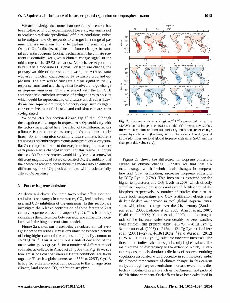
Figure2a shows our present-day calculated annual aver-age isoprene emissions. Emissions show the expected patternof being highest around the tropics, and globally amount to467 TgCyr−1. This is within one standard deviation of themean value (515 TgCyr−1) for a number of different modelestimates as collated inArneth et al.(2008). In Fig.2b we seehow emissions change when all future conditions are takentogether. There is a global decrease of 55 % to 208 TgCyr−1.In Fig. 2c–e the individual contributions to this change fromclimate, land use and CO2 inhibition are given.

Discussion

Paper

|D

iscussionP

aper|

Discussion

Paper

|D

iscussionP

aper|

Discu

ssionPaper

|Discu

ssionPaper

|Discu

ssionPaper

|Discu

ssionPaper

|

Latit

ude

Longitude

−90° 0° 90° 180°

−40°

−20°

0°

20°

40°

(a) Present Day (467 Tg C yr−1) (b) 2095 (All factors) (208 Tg C yr−1)

0 0.5 1 1.5 2 >2.5

Latit

ude

−40°

−20°

0°

20°

40°

(c) ∆ Climate (+78.2 Tg C yr−1) (d) ∆ Land use (−190 Tg C yr−1)

−40°

−20°

0°

20°

40°

(e) ∆ CO2 inhibition (−225 Tg C yr−1)

−90° 0° 90° 180°

(f) ∆ All factors (−259 Tg C yr−1)

<−2.5 −2 −1.5 −1 −0.5 0 0.5 1 1.5 2 >2.5

Fig. 1. Isoprene emissions (mg C m-2 hr-1) generated using the SDGVM and a biogenic emis-sions model. (a) Present day (2000), (b) with 2095 climate, land use and CO2 inhibition, (c-e)change caused by each factor, (f) change with all factors combined. Quoted are total globalisoprene emissions (a-b) and the change in this value (c-e).

30

Fig. 2. Isoprene emissions (mgCm−2 hr−1) generated using the SDGVM and a biogenic emis-sions model. (a) Present day (2000), (b) with 2095 climate, land use and CO2 inhibition, (c–e)change caused by each factor, (f) change with all factors combined. Quoted in the plot titles aretotal global isoprene emissions (a–b) and the change in this value (c–e).

35

Fig. 2. Isoprene emissions (mgCm−2h−1) generated using theSDGVM and a biogenic emissions model.(a) Present-day (2000),(b) with 2095 climate, land use and CO2 inhibition, (c–e)changecaused by each factor,(f) change with all factors combined. Quotedin the plot titles are total global isoprene emissions(a–b) and thechange in this value(c–e).

Figure 2c shows the difference in isoprene emissionscaused by climate change. Globally we find that cli-mate change, which includes both changes in tempera-ture and CO2 fertilisation, increases isoprene emissionsby 78 TgCyr−1 (17 %). This increase is expected for thehigher temperatures and CO2 levels in 2095, which directlystimulate isoprene emissions and extend fertilisation of thebiosphere respectively. A number of studies that also in-clude both temperature and CO2 fertilisation effects sim-ilarly calculate an increase in total global isoprene emis-sions with climate change over the 21st century (Sander-son et al., 2003; Lathière et al., 2005; Arneth et al., 2007;Heald et al., 2009; Young et al., 2009), but the magni-tude of the increase varies considerably between studies.Four studies (this present study (+17 %, +78 TgCyr−1),Sanderson et al.(2003) (+21 %,+131 TgCyr−1), Lathièreet al.(2005) (+27 %,+136 TgCyr−1) andWu et al.(2012)(+25 %,+103 TgCyr−1)) calculate moderate increases. Thethree other studies calculate significantly higher values. Themain source of discrepancy is the extent to which, in cer-tain regions, models simulate a die-back of isoprene emittingvegetation associated with a decrease in soil moisture underthe elevated temperatures of climate change. In this currentstudy, although isoprene emissions increase overall, this die-back is calculated in areas such as the Amazon and parts ofthe Maritime continent. Such effects have been calculated in



previous studies (Cox et al., 2000; Sanderson et al., 2003;Lathière et al., 2005). In some other studies 2100 soil mois-ture is high enough to avoid large-scale die-back, and subse-quently their calculated increases in isoprene emissions aremuch higher (e.g.Heald et al., 2009, calculate increases of1344 TgCyr−1 (265 %)).

Figure2d shows the effect of future land use change onisoprene emissions. In those areas most affected by land usechange, a decrease in isoprene emissions is calculated. Thisis a result of the cropland expansion scenario we employ inwhich broad-leaved trees are replaced with lower isopreneemitting crops. The spatial distribution of these vegetationchanges is shown in Fig.1.

Figure1a shows the change in C3 grasses (to which cropswere assigned) calculated using the IMAGE model for 2095.The main areas of cropland expansion are the Amazon,central Africa, Southeast Asia, USA, and northern Eura-sia. However only the tropical regions and southeast USAshow decreases in isoprene emissions. In these regions crop-land expansion occurs at the expense of broad-leaved trees(Fig. 1b). Little change in isoprene emissions is calculatedover the rest of the USA and northern Eurasia, as here onelow isoprene emitting LST (crops) is replaced by another(largely bare soil – Fig.1c). Wu et al.(2012) also calculatethat future land use following the A1B scenario causes a de-crease in end of 21st century isoprene emissions comparedto the future case with present-day land use. However theycalculate a smaller decrease of only−67 TgCyr−1 globally.The use of a different vegetation model (LPJ-DGVM) is a po-tential source of discrepancy.

The inhibition of isoprene emissions by CO2 (Fig. 2e) in-creases by 2095 due to the greater CO2 levels in the atmo-sphere in the B2 scenario (+251 ppm,+60 %). Decreases inisoprene emissions occur wherever isoprene is emitted, andare largest where emissions are highest. Globally this leadsto greater decreases in isoprene emissions (−225 TgCyr−1,48 %) than for land use change (−190 Tgyr−1). It should benoted though that the value of−225 TgCyr−1 is calculatedfor the case with future climate change but not land use, i.e.under a scenario where isoprene emissions and CO2 are high.It is for this reason that the values quoted in Fig.2c–e do notadd up to the value for the combined impact in Fig.2f. Whenland use change is also taken into account, the effect of CO2inhibition is reduced to−147 TgCyr−1 and the values do addup to the combined impact.

The combined effect of changes in climate, land use, andCO2 inhibition of isoprene emissions is shown in Fig.2f.Overall there is a decrease in global isoprene emissions(−259 TgCyr−1). Land use change (−190 TgCyr−1) andCO2 inhibition (−147 TgCyr−1) both contribute signifi-cantly to the net change in isoprene emissions. These con-tributions outweigh those of increased temperatures andCO2 fertilisation (+78 TgCyr−1). Other studies have foundthat land use change (e.g. Wu et al., 2012) or CO2 inhibi-tion (e.g. Heald et al., 2009; Young et al., 2009; Arneth et al.,

2007b) can separately compensate for the isoprene emissionincrease caused by temperature and CO2 fertilisation over the21st century, leaving little overall change in global isopreneemissions since present-day. Assuming, as in our study, thatthe land use scenario projects an overall decrease in isopreneemitters, it follows that the combined effect of both landuse change and CO2 inhibition should lead to a decrease inglobal isoprene emissions as found here. It is important tonote though that as calculating future global isoprene emis-sion changes involves a number of terms, each of which isuncertain, the overall balance between these terms has a highdegree of uncertainty.

4 Attribution of changes in future ozone

In this section the results of the UM-UKCA integrations areanalysed in order to attribute changes in O3 over the 21st cen-tury to changes in climate, isoprene emissions with climate,anthropogenic emissions, land use and CO2 inhibition of iso-prene emissions. Prior to the analysis we briefly evaluate thetropospheric O3 calculated by UM-UKCA by comparison tomeasurements.

4.1 Model evaluation

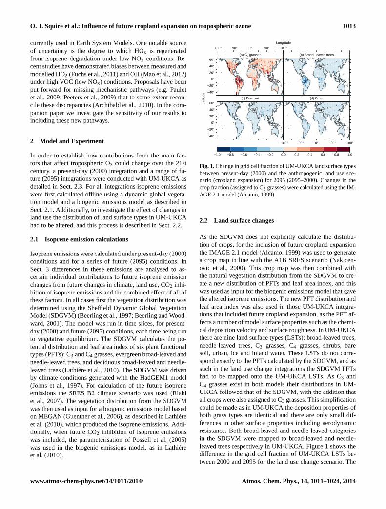
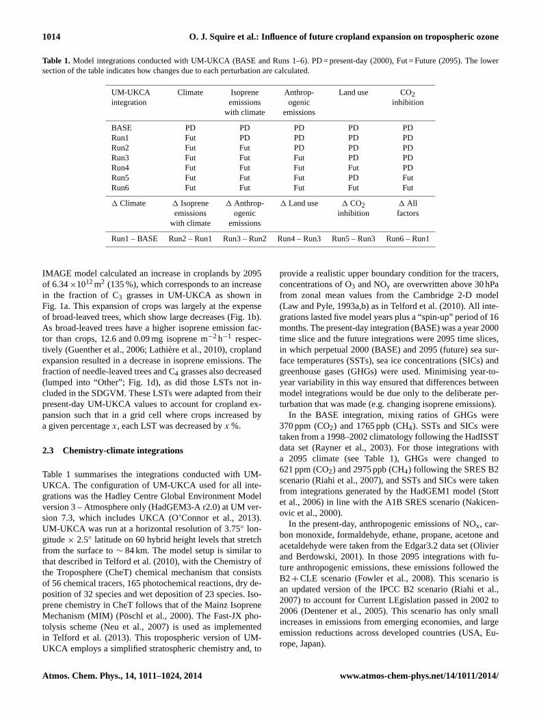
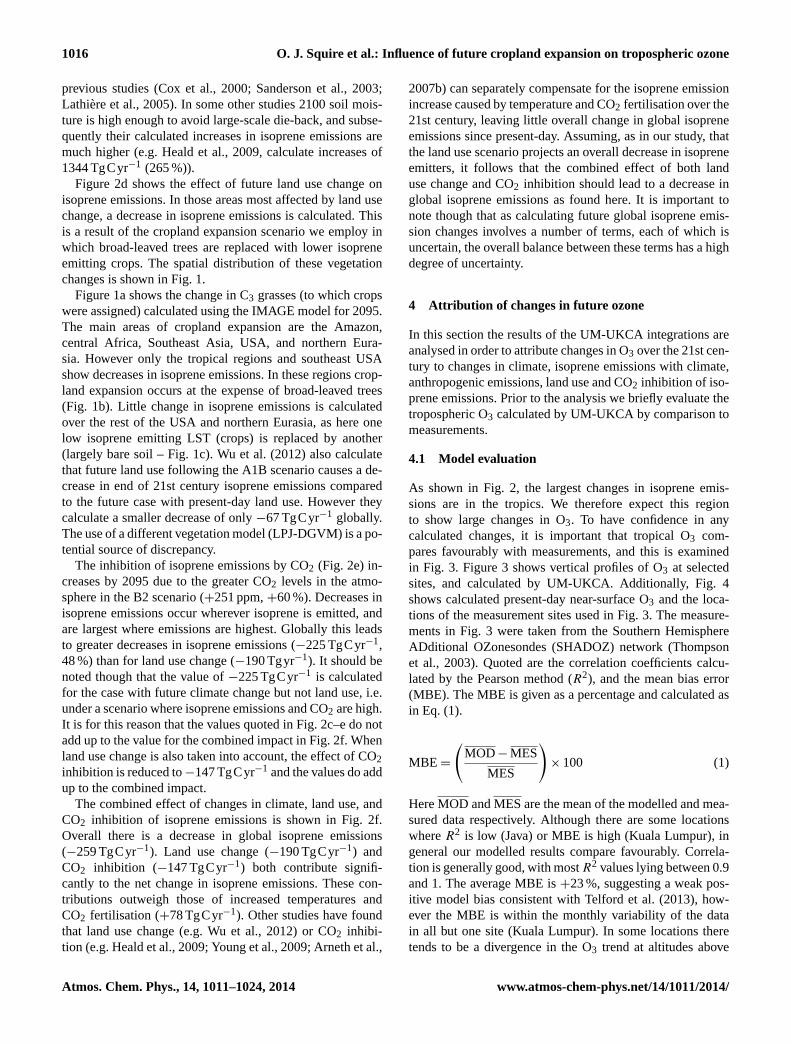
As shown in Fig.2, the largest changes in isoprene emis-sions are in the tropics. We therefore expect this regionto show large changes in O3. To have confidence in anycalculated changes, it is important that tropical O3 com-pares favourably with measurements, and this is examinedin Fig. 3. Figure3 shows vertical profiles of O3 at selectedsites, and calculated by UM-UKCA. Additionally, Fig.4shows calculated present-day near-surface O3 and the loca-tions of the measurement sites used in Fig.3. The measure-ments in Fig.3 were taken from the Southern HemisphereADditional OZonesondes (SHADOZ) network (Thompsonet al., 2003). Quoted are the correlation coefficients calcu-lated by the Pearson method (R2), and the mean bias error(MBE). The MBE is given as a percentage and calculated asin Eq. (1).

MBE =

(MOD − MES

MES

)× 100 (1)

HereMOD andMES are the mean of the modelled and mea-sured data respectively. Although there are some locationswhereR2 is low (Java) or MBE is high (Kuala Lumpur), ingeneral our modelled results compare favourably. Correla-tion is generally good, with mostR2 values lying between 0.9and 1. The average MBE is+23 %, suggesting a weak pos-itive model bias consistent withTelford et al.(2013), how-ever the MBE is within the monthly variability of the datain all but one site (Kuala Lumpur). In some locations theretends to be a divergence in the O3 trend at altitudes above


O. J. Squire et al.: Influence of future cropland expansion on tropospheric ozone 1017Discussion

Pa

per|

Discussion

Paper

|D

iscussionP

aper|

Discussion

Paper

|

Ozone (ppb)

Alti

tude

(hPa

)

900

700

500

250R2=0.878, MBE= 9.9

Samoa

0 20 40 60 80 100

R2=0.952, MBE=25.9Hilo

R2=0.867, MBE=31.2San Cristobal

0 20 40 60 80 100

R2=0.919, MBE=20.3Heredia

R2=0.945, MBE=21.2Natal

R2=0.942, MBE=10.6Ascension

R2=0.791, MBE= 5.5Cotonou

900

700

500

250R2=0.987, MBE=−2.1

Irene

900

700

500

250

0 20 40 60 80 100

R2=0.991, MBE=−5.5Malindi

R2=0.992, MBE=−1.0Reunion

0 20 40 60 80 100

R2=0.898, MBE=40.8Kuala Lumpar

R2=0.099, MBE=22.6Java

Fig. 3. Five year mean O3 (ppb) from the BASE run (red) compared to O3 sonde data from theSHADOZ Network (Thompson et˜al., 2003) (black). Polygons show extent of monthly variability.Correlation coefficients (R2) are calculated using the Pearson method. Mean bias errors (MBE)are in %; positive values indicate the model is biased high with respect to the measurementdata.

32

Fig. 3. Five year mean O3 (ppb) from the BASE run (red) compared to O3 sonde data from theSHADOZ Network (Thompson et al., 2003) (black). Polygons show extent of monthly variability.Correlation coefficients (R2) are calculated using the Pearson method. Mean bias errors (MBE)are in %; positive values indicate the model is biased high with respect to the measurementdata.

36

Fig. 3. Five-year mean O3 (ppb) from the BASE run (red) compared to O3 sonde data from the SHADOZ Network (Thompson et al., 2003)(black). Polygons show extent of monthly variability. Correlation coefficients (R2) are calculated using the Pearson method. Mean bias errors(MBE) are in %; positive values indicate the model is biased high with respect to the measurement data.

Table 2. Changes in the Ox budget (Tgyr−1) from the present-day BASE integration caused by the change in various factors betweenpresent-day and 2095. Also quoted are changes in the O3 burden (Tg). Percentage changes are in brackets.

Tgyr−1 Prod Loss Net Chem Influx Dry Dep Burden (Tg)

BASE 6188 5602 586 673 1259 379

1 Climate +393 (+6) +546 (+10) −153 (−26) +144 (+21) −8 (−1) +7 (+2)1 Isoprene Ems +56 (+1) +64 (+1) −8 (−1) +15 (+2) +6 (0) +3 (+1)(with 1 climate)1 Anthrop Ems −199 (−3) −118 (−2) −81 (−14) +33 (+5) −48 (−4) −4 (−1)1 Land Use −286 (−5) −296 (−5) +10 (+2) −45 (−7) −35 (−3) −19 (−5)1 CO2 Inhibition −270 (−4) −284 (−5) +14 (+2) −46 (−7) −32 (−3) −16 (−4)1 All factors −263 (−4) −33 (−1) −230 (−39) +116 (+17) −115 (−9) −27 (−7)

∼ 500 hPa, however this is not generally the case at loweraltitudes, which are more pertinent to this study.

The near-surface O3 modelled by UM-UKCA in Fig.4generally shows higher O3 in the Northern Hemisphere withpeaks over the Mediterranean and Middle East, coastal USA,Tibetan Plateau and the region of the East China Sea. Lowsare over remote oceanic regions, most pronounced over theWestern Pacific, and the rainforests (most notably the Ama-zon). This spatial pattern and the magnitude of troposphericO3 compares favourably to the ACCMIP ensemble mean in

Young et al.(2013). For a more extensive evaluation of UM-UKCA seeTelford et al.(2010) andO’Connor et al.(2013).

4.2 Ozone changes

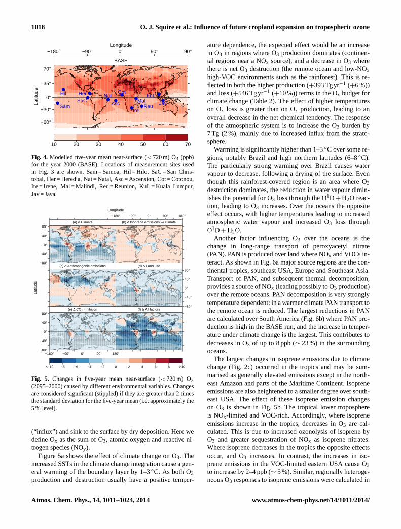
Figure5 shows how the near-surface tropospheric O3 mixingratio changes between 2000 and 2095 in the UM-UKCA in-tegrations as caused by the different environmental variablesmentioned previously. In Table2 we report Ox budgets forthe integrations, which compare tropospheric chemical pro-duction and loss of Ox with its source from the stratosphere



Discussion

Paper

|D

iscussionP

aper|

Discussion

Paper

|D

iscussionP

aper|

Discu

ssionPaper

|Discu

ssionPaper

|Discu

ssionPaper

|Discu

ssionPaper

|

Latit

ude

Longitude−180° −90° 0° 90° 90°

−60°

−30°

0°

35°

70°

●Sam

●Hil

●SaC

●Her●

Nat●

Asc

●Cot

●Mal●Ire

●Reu

●KuL●

Jav

BASE

10 20 30 40 50 60 70

Fig. 4. Modelled five year mean near surface (<720 m) O3 (ppb) for the year 2000 (BASE).Locations of measurement sites used in Figure 3 are shown. Sam = Samoa, Hil = Hilo, SaC =San Christobal, Her = Heredia, Nat = Natal, Asc = Ascension, Cot = Cotonou, Ire = Irene, Mal= Malindi, Reu = Reunion, KuL = Kuala Lumpar, Jav = Java.

33

Fig. 4. Modelled five year mean near surface (< 720 m) O3 (ppb) for the year 2000(BASE). Locations of measurement sites used in Fig. 3 are shown. Sam=Samoa, Hil=Hilo,SaC=San Christobal, Her=Heredia, Nat=Natal, Asc=Ascension, Cot=Cotonou, Ire= Irene,Mal=Malindi, Reu=Reunion, KuL=Kuala Lumpar, Jav= Java.

37

Fig. 4. Modelled five-year mean near-surface (< 720 m) O3 (ppb)for the year 2000 (BASE). Locations of measurement sites usedin Fig. 3 are shown. Sam = Samoa, Hil = Hilo, SaC = San Chris-tobal, Her = Heredia, Nat = Natal, Asc = Ascension, Cot = Cotonou,Ire = Irene, Mal = Malindi, Reu = Reunion, KuL = Kuala Lumpur,Jav = Java.

Discussion

Paper

|D

iscussionP

aper|

Discussion

Paper

|D

iscussionP

aper|

Latit

ude

Longitude

−80°

−40°

0°

40°

80°(a) ∆ Climate

−180° −90° 0° 90° 180°

(b) ∆ Isoprene emissions w/ climate

(c) ∆ Anthropogenic emissions

−80°

−40°

0°

40°

80°(d) ∆ Land use

−80°

−40°

0°

40°

80°

−180° −90° 0° 90° 180°

(e) ∆ CO2 Inhibition (f) ∆ All factors

<−10 −8 −6 −4 −2 0 2 4 6 8 >10

Fig. 5. Changes in five year mean near surface (< 720 m) O3 (2095 – 2000) caused by differentenvironmental variables. Changes are considered significant (stippled) if they are greater than2 times the standard deviation for the five year mean (i.e. approximately the 5 % level).

38

Fig. 5. Changes in five-year mean near-surface (< 720 m) O3(2095–2000) caused by different environmental variables. Changesare considered significant (stippled) if they are greater than 2 timesthe standard deviation for the five-year mean (i.e. approximately the5 % level).

(“influx”) and sink to the surface by dry deposition. Here wedefine Ox as the sum of O3, atomic oxygen and reactive ni-trogen species (NOy).

Figure5a shows the effect of climate change on O3. Theincreased SSTs in the climate change integration cause a gen-eral warming of the boundary layer by 1–3◦C. As both O3production and destruction usually have a positive temper-

ature dependence, the expected effect would be an increasein O3 in regions where O3 production dominates (continen-tal regions near a NOx source), and a decrease in O3 wherethere is net O3 destruction (the remote ocean and low-NOxhigh-VOC environments such as the rainforest). This is re-flected in both the higher production (+393 Tgyr−1 (+6 %))and loss (+546 Tgyr−1 (+10 %)) terms in the Ox budget forclimate change (Table2). The effect of higher temperatureson Ox loss is greater than on Ox production, leading to anoverall decrease in the net chemical tendency. The responseof the atmospheric system is to increase the O3 burden by7 Tg (2 %), mainly due to increased influx from the strato-sphere.

Warming is significantly higher than 1–3◦C over some re-gions, notably Brazil and high northern latitudes (6–8◦C).The particularly strong warming over Brazil causes watervapour to decrease, following a drying of the surface. Eventhough this rainforest-covered region is an area where O3destruction dominates, the reduction in water vapour dimin-ishes the potential for O3 loss through the O1D + H2O reac-tion, leading to O3 increases. Over the oceans the oppositeeffect occurs, with higher temperatures leading to increasedatmospheric water vapour and increased O3 loss throughO1D + H2O.

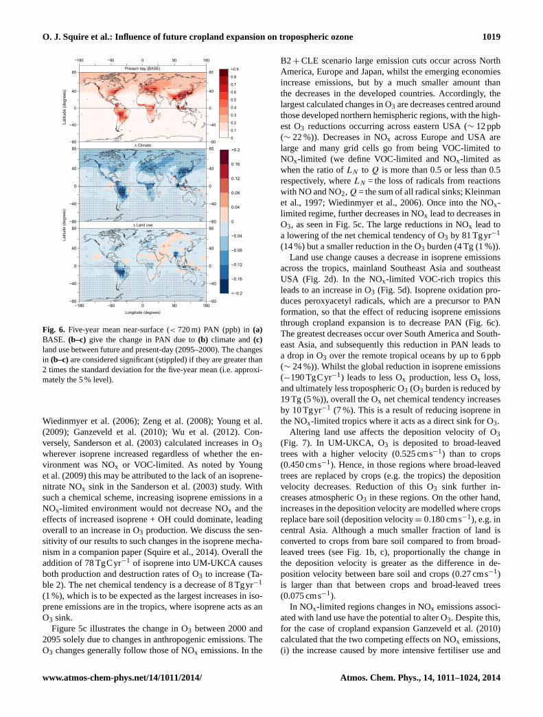
Another factor influencing O3 over the oceans is thechange in long-range transport of peroxyacetyl nitrate(PAN). PAN is produced over land where NOx and VOCs in-teract. As shown in Fig.6a major source regions are the con-tinental tropics, southeast USA, Europe and Southeast Asia.Transport of PAN, and subsequent thermal decomposition,provides a source of NOx (leading possibly to O3 production)over the remote oceans. PAN decomposition is very stronglytemperature dependent; in a warmer climate PAN transport tothe remote ocean is reduced. The largest reductions in PANare calculated over South America (Fig.6b) where PAN pro-duction is high in the BASE run, and the increase in temper-ature under climate change is the largest. This contributes todecreases in O3 of up to 8 ppb (∼ 23 %) in the surroundingoceans.

The largest changes in isoprene emissions due to climatechange (Fig.2c) occurred in the tropics and may be sum-marised as generally elevated emissions except in the north-east Amazon and parts of the Maritime Continent. Isopreneemissions are also heightened to a smaller degree over south-east USA. The effect of these isoprene emission changeson O3 is shown in Fig.5b. The tropical lower troposphereis NOx-limited and VOC-rich. Accordingly, where isopreneemissions increase in the tropics, decreases in O3 are cal-culated. This is due to increased ozonolysis of isoprene byO3 and greater sequestration of NOx as isoprene nitrates.Where isoprene decreases in the tropics the opposite effectsoccur, and O3 increases. In contrast, the increases in iso-prene emissions in the VOC-limited eastern USA cause O3to increase by 2–4 ppb (∼ 5 %). Similar, regionally heteroge-neous O3 responses to isoprene emissions were calculated in



Discussion

Paper

|D

iscussionP

aper|

Discussion

Paper

|D

iscussionP

aper|

Latit

ude

(deg

rees

)−180 −90 0 90 180

−80

−40

0

40

85

−80

−40

0

40

85Present day (BASE)

0

0.1

0.2

0.3

0.4

0.5

0.6

0.7

0.8

>0.9

Longitude (degrees)

Latit

ude

(deg

rees

)

−80

−40

0

40

85

−80

−40

0

40

85∆ Climate

−80

−40

0

40

85

−180 −90 0 90 180−80

−40

0

40

85∆ Land use

<−0.2

−0.16

−0.12

−0.08

−0.04

0

0.04

0.08

0.12

0.16

>0.2

Fig. 6. Five year mean near surface (<720 m) PAN (ppb) in (a) BASE. (b-c) give the changein PAN due to (b) climate and (c) land use between future and present day (2095 - 2000).The changes in (b-c) are considered significant (stippled) if they are greater than 2 times thestandard deviation for the five year mean (i.e. approximately the 5 % level).

35

Fig. 6. Five year mean near surface (< 720 m) PAN (ppb) in (a) BASE. (b–c) give the changein PAN due to (b) climate and (c) land use between future and present day (2095–2000).The changes in (b–c) are considered significant (stippled) if they are greater than 2 times thestandard deviation for the five year mean (i.e. approximately the 5 % level).

39

Fig. 6. Five-year mean near-surface (< 720 m) PAN (ppb) in(a)BASE. (b–c) give the change in PAN due to(b) climate and(c)land use between future and present-day (2095–2000). The changesin (b–c)are considered significant (stippled) if they are greater than2 times the standard deviation for the five-year mean (i.e. approxi-mately the 5 % level).

Wiedinmyer et al.(2006); Zeng et al.(2008); Young et al.(2009); Ganzeveld et al.(2010); Wu et al. (2012). Con-versely,Sanderson et al.(2003) calculated increases in O3wherever isoprene increased regardless of whether the en-vironment was NOx or VOC-limited. As noted byYounget al.(2009) this may be attributed to the lack of an isoprene-nitrate NOx sink in theSanderson et al.(2003) study. Withsuch a chemical scheme, increasing isoprene emissions in aNOx-limited environment would not decrease NOx and theeffects of increased isoprene + OH could dominate, leadingoverall to an increase in O3 production. We discuss the sen-sitivity of our results to such changes in the isoprene mecha-nism in a companion paper (Squire et al., 2014). Overall theaddition of 78 TgCyr−1 of isoprene into UM-UKCA causesboth production and destruction rates of O3 to increase (Ta-ble 2). The net chemical tendency is a decrease of 8 Tgyr−1

(1 %), which is to be expected as the largest increases in iso-prene emissions are in the tropics, where isoprene acts as anO3 sink.

Figure5c illustrates the change in O3 between 2000 and2095 solely due to changes in anthropogenic emissions. TheO3 changes generally follow those of NOx emissions. In the

B2+ CLE scenario large emission cuts occur across NorthAmerica, Europe and Japan, whilst the emerging economiesincrease emissions, but by a much smaller amount thanthe decreases in the developed countries. Accordingly, thelargest calculated changes in O3 are decreases centred aroundthose developed northern hemispheric regions, with the high-est O3 reductions occurring across eastern USA (∼ 12 ppb(∼ 22 %)). Decreases in NOx across Europe and USA arelarge and many grid cells go from being VOC-limited toNOx-limited (we define VOC-limited and NOx-limited aswhen the ratio ofLN to Q is more than 0.5 or less than 0.5respectively, whereLN = the loss of radicals from reactionswith NO and NO2, Q = the sum of all radical sinks;Kleinmanet al., 1997; Wiedinmyer et al., 2006). Once into the NOx-limited regime, further decreases in NOx lead to decreases inO3, as seen in Fig.5c. The large reductions in NOx lead toa lowering of the net chemical tendency of O3 by 81 Tgyr−1

(14 %) but a smaller reduction in the O3 burden (4 Tg (1 %)).Land use change causes a decrease in isoprene emissions

across the tropics, mainland Southeast Asia and southeastUSA (Fig. 2d). In the NOx-limited VOC-rich tropics thisleads to an increase in O3 (Fig. 5d). Isoprene oxidation pro-duces peroxyacetyl radicals, which are a precursor to PANformation, so that the effect of reducing isoprene emissionsthrough cropland expansion is to decrease PAN (Fig.6c).The greatest decreases occur over South America and South-east Asia, and subsequently this reduction in PAN leads toa drop in O3 over the remote tropical oceans by up to 6 ppb(∼ 24 %)). Whilst the global reduction in isoprene emissions(−190 TgCyr−1) leads to less Ox production, less Ox loss,and ultimately less tropospheric O3 (O3 burden is reduced by19 Tg (5 %)), overall the Ox net chemical tendency increasesby 10 Tgyr−1 (7 %). This is a result of reducing isoprene inthe NOx-limited tropics where it acts as a direct sink for O3.

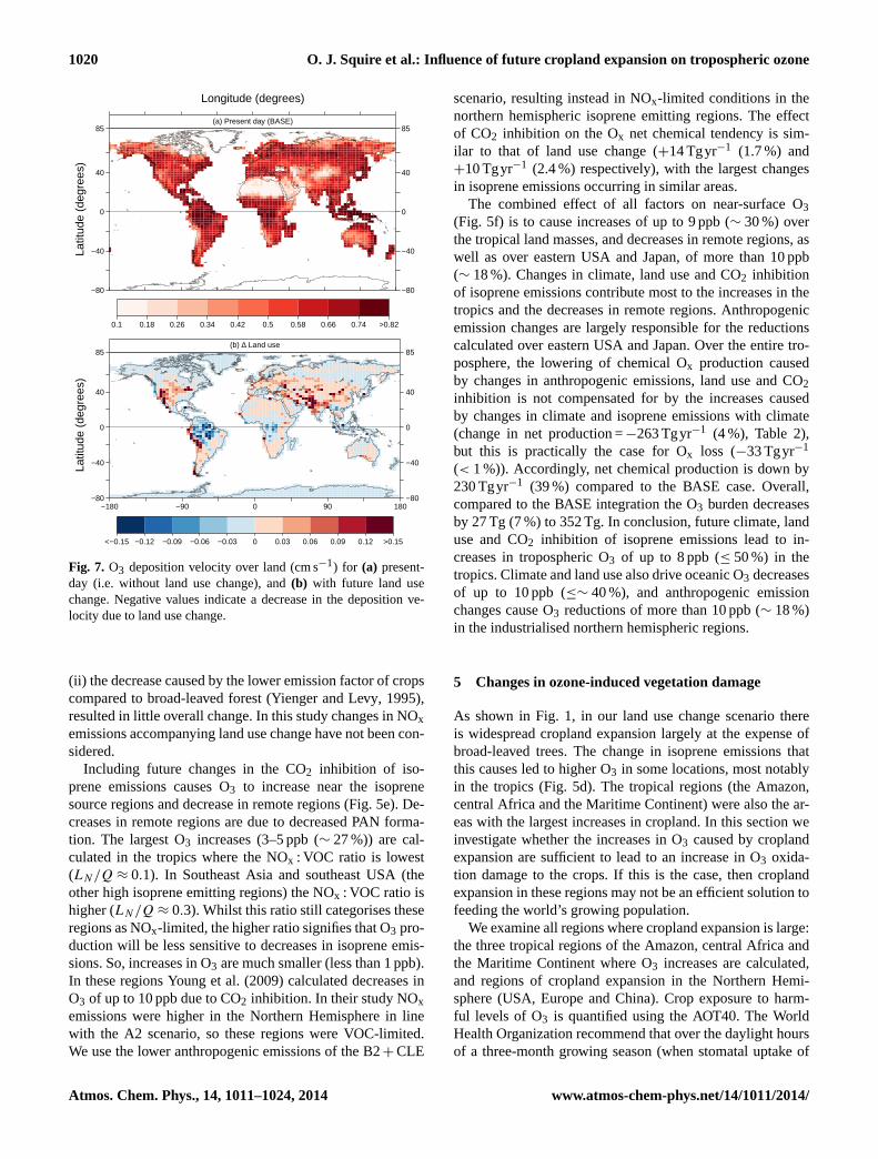
Altering land use affects the deposition velocity of O3(Fig. 7). In UM-UKCA, O3 is deposited to broad-leavedtrees with a higher velocity (0.525 cms−1) than to crops(0.450 cms−1). Hence, in those regions where broad-leavedtrees are replaced by crops (e.g. the tropics) the depositionvelocity decreases. Reduction of this O3 sink further in-creases atmospheric O3 in these regions. On the other hand,increases in the deposition velocity are modelled where cropsreplace bare soil (deposition velocity= 0.180 cms−1), e.g. incentral Asia. Although a much smaller fraction of land isconverted to crops from bare soil compared to from broad-leaved trees (see Fig.1b, c), proportionally the change inthe deposition velocity is greater as the difference in de-position velocity between bare soil and crops (0.27 cms−1)is larger than that between crops and broad-leaved trees(0.075 cms−1).

In NOx-limited regions changes in NOx emissions associ-ated with land use have the potential to alter O3. Despite this,for the case of cropland expansionGanzeveld et al.(2010)calculated that the two competing effects on NOx emissions,(i) the increase caused by more intensive fertiliser use and



Discussion

Paper

|D

iscussionP

aper|

Discussion

Paper

|D

iscussionP

aper|

Discu

ssionPaper

|Discu

ssionPaper

|Discu

ssionPaper

|Discu

ssionPaper

|

Latit

ude

(deg

rees

)

Longitude (degrees)

−80

−40

0

40

85

−80

−40

0

40

85(a) Present day (BASE)

0.1 0.18 0.26 0.34 0.42 0.5 0.58 0.66 0.74 >0.82

Latit

ude

(deg

rees

)

−80

−40

0

40

85

−180 −90 0 90 180−80

−40

0

40

85(b) ∆ Land use

<−0.15 −0.12 −0.09 −0.06 −0.03 0 0.03 0.06 0.09 0.12 >0.15

Fig. 7. O3 deposition velocity (cm s-1) for (a) present day (i.e. without land use change), and(b) with future land use change. Negative values indicate a decrease in the deposition velocitydue to land use change.

36

Fig. 7. O3 deposition velocity over land (cm s−1) for (a) present day (i.e. without land usechange), and (b) with future land use change. Negative values indicate a decrease in the de-position velocity due to land use change.

40

Fig. 7. O3 deposition velocity over land (cm s−1) for (a) present-day (i.e. without land use change), and(b) with future land usechange. Negative values indicate a decrease in the deposition ve-locity due to land use change.

(ii) the decrease caused by the lower emission factor of cropscompared to broad-leaved forest (Yienger and Levy, 1995),resulted in little overall change. In this study changes in NOxemissions accompanying land use change have not been con-sidered.

Including future changes in the CO2 inhibition of iso-prene emissions causes O3 to increase near the isoprenesource regions and decrease in remote regions (Fig.5e). De-creases in remote regions are due to decreased PAN forma-tion. The largest O3 increases (3–5 ppb (∼ 27 %)) are cal-culated in the tropics where the NOx : VOC ratio is lowest(LN/Q ≈ 0.1). In Southeast Asia and southeast USA (theother high isoprene emitting regions) the NOx : VOC ratio ishigher (LN/Q ≈ 0.3). Whilst this ratio still categorises theseregions as NOx-limited, the higher ratio signifies that O3 pro-duction will be less sensitive to decreases in isoprene emis-sions. So, increases in O3 are much smaller (less than 1 ppb).In these regionsYoung et al.(2009) calculated decreases inO3 of up to 10 ppb due to CO2 inhibition. In their study NOxemissions were higher in the Northern Hemisphere in linewith the A2 scenario, so these regions were VOC-limited.We use the lower anthropogenic emissions of the B2+ CLE

scenario, resulting instead in NOx-limited conditions in thenorthern hemispheric isoprene emitting regions. The effectof CO2 inhibition on the Ox net chemical tendency is sim-ilar to that of land use change (+14 Tgyr−1 (1.7 %) and+10 Tgyr−1 (2.4 %) respectively), with the largest changesin isoprene emissions occurring in similar areas.

The combined effect of all factors on near-surface O3(Fig. 5f) is to cause increases of up to 9 ppb (∼ 30 %) overthe tropical land masses, and decreases in remote regions, aswell as over eastern USA and Japan, of more than 10 ppb(∼ 18 %). Changes in climate, land use and CO2 inhibitionof isoprene emissions contribute most to the increases in thetropics and the decreases in remote regions. Anthropogenicemission changes are largely responsible for the reductionscalculated over eastern USA and Japan. Over the entire tro-posphere, the lowering of chemical Ox production causedby changes in anthropogenic emissions, land use and CO2inhibition is not compensated for by the increases causedby changes in climate and isoprene emissions with climate(change in net production =−263 Tgyr−1 (4 %), Table2),but this is practically the case for Ox loss (−33 Tgyr−1

(< 1 %)). Accordingly, net chemical production is down by230 Tgyr−1 (39 %) compared to the BASE case. Overall,compared to the BASE integration the O3 burden decreasesby 27 Tg (7 %) to 352 Tg. In conclusion, future climate, landuse and CO2 inhibition of isoprene emissions lead to in-creases in tropospheric O3 of up to 8 ppb (≤ 50 %) in thetropics. Climate and land use also drive oceanic O3 decreasesof up to 10 ppb (≤∼ 40 %), and anthropogenic emissionchanges cause O3 reductions of more than 10 ppb (∼ 18 %)in the industrialised northern hemispheric regions.

5 Changes in ozone-induced vegetation damage

As shown in Fig.1, in our land use change scenario thereis widespread cropland expansion largely at the expense ofbroad-leaved trees. The change in isoprene emissions thatthis causes led to higher O3 in some locations, most notablyin the tropics (Fig.5d). The tropical regions (the Amazon,central Africa and the Maritime Continent) were also the ar-eas with the largest increases in cropland. In this section weinvestigate whether the increases in O3 caused by croplandexpansion are sufficient to lead to an increase in O3 oxida-tion damage to the crops. If this is the case, then croplandexpansion in these regions may not be an efficient solution tofeeding the world’s growing population.

We examine all regions where cropland expansion is large:the three tropical regions of the Amazon, central Africa andthe Maritime Continent where O3 increases are calculated,and regions of cropland expansion in the Northern Hemi-sphere (USA, Europe and China). Crop exposure to harm-ful levels of O3 is quantified using the AOT40. The WorldHealth Organization recommend that over the daylight hoursof a three-month growing season (when stomatal uptake of



Discussion

Pa

per|

Discussion

Paper

|D

iscussionP

aper|

Discussion

Paper

|

Discu

ssionPaper

|Discu

ssionPaper

|Discu

ssionPaper

|Discu

ssionPaper

|

Longitude (°)

Latit

ude

(°) 20

3040

50

−120 −100 −80

●

●

●

●

●● ● ●● ● ● ●

● ● ● ●● ● ● ● ● ●

●●

●

●

● ●

●●

●

●

●

●●

●● ●

● ● ●● ● ●

● ●

(a) USA (MJJ)

3040

5060

70

0 20 40●

●

●

●

●● ● ●● ● ● ●

● ● ● ●● ● ● ● ● ●

●●

●

●

●● ● ●

●●

●

●

●

●●

●● ●

● ● ●● ● ●

● ● ● ●● ● ●

(b) Europe (AMJ)

2530

3540

45

80 100 120 140●

●

●

●

●

●

●

●

●

● ● ●

●

●

●

●

●

●

● ●

● ● ●

● ● ●

● ● ● ●

● ● ●

(c) China (JJA)

−30

−20

−10

010

−80 −70 −60 −50 −40

●

●

●

●● ● ●● ● ● ●

● ● ● ●● ● ● ● ● ●

●●

●

●

● ●

●●

●

●

●

●●

●● ●

● ● ●● ● ●

● ●(d) Brazil (DJF)

−20

−10

010

10 20 30 40

●

●

●● ● ●● ● ● ●

● ● ● ●● ● ● ● ● ●

●

●●

●

●● ●

● ●●(e) Africa (JFM)

−10

010

20

100 120 140 160

●

●

●

●● ● ●● ● ● ●

● ● ● ●● ● ● ● ● ●

●●

●

●

●● ● ●

●●

●

●

●

●●

●● ●

● ● ●● ● ●

● ● ● ●● ● ●

(f) Maritime Cont. (NDJ)

<−5

−4

−3

−2

−1

0

1

2

3

4

>5

Fig. 8. Change in AOT40 >3 ppm hr during the daylights hours of the regional 3 month growingseason caused by cropland expansion. Growing seasons are quoted e.g. MJJ = May, June,July. White areas are where both without and with cropland expansion the AOT40 is belowthe threshold. Green circles indicate crossing to below the threshold. Gold triangles indicatecrossing to above the threshold.

37

Fig. 8. Change in AOT40> 3 ppm h during the daylights hours of the regional 3 month growingseason caused by cropland expansion. Growing seasons are quoted e.g. MJJ=May, June,July. White areas are where both without and with cropland expansion the AOT40 is belowthe threshold. Green circles indicate crossing to below the threshold. Gold triangles indicatecrossing to above the threshold.

41

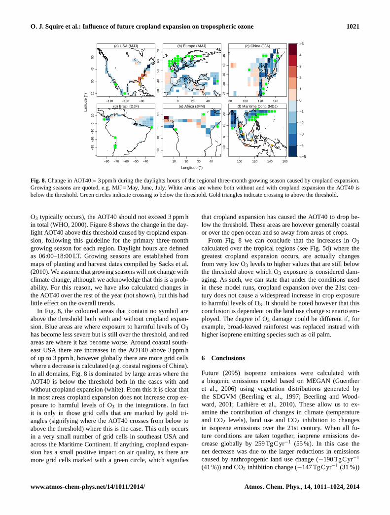
Fig. 8. Change in AOT40> 3 ppm h during the daylights hours of the regional three-month growing season caused by cropland expansion.Growing seasons are quoted, e.g. MJJ = May, June, July. White areas are where both without and with cropland expansion the AOT40 isbelow the threshold. Green circles indicate crossing to below the threshold. Gold triangles indicate crossing to above the threshold.

O3 typically occurs), the AOT40 should not exceed 3 ppm hin total (WHO, 2000). Figure8 shows the change in the day-light AOT40 above this threshold caused by cropland expan-sion, following this guideline for the primary three-monthgrowing season for each region. Daylight hours are definedas 06:00–18:00 LT. Growing seasons are established frommaps of planting and harvest dates compiled bySacks et al.(2010). We assume that growing seasons will not change withclimate change, although we acknowledge that this is a prob-ability. For this reason, we have also calculated changes inthe AOT40 over the rest of the year (not shown), but this hadlittle effect on the overall trends.

In Fig. 8, the coloured areas that contain no symbol areabove the threshold both with and without cropland expan-sion. Blue areas are where exposure to harmful levels of O3has become less severe but is still over the threshold, and redareas are where it has become worse. Around coastal south-east USA there are increases in the AOT40 above 3 ppm hof up to 3 ppm h, however globally there are more grid cellswhere a decrease is calculated (e.g. coastal regions of China).In all domains, Fig.8 is dominated by large areas where theAOT40 is below the threshold both in the cases with andwithout cropland expansion (white). From this it is clear thatin most areas cropland expansion does not increase crop ex-posure to harmful levels of O3 in the integrations. In factit is only in those grid cells that are marked by gold tri-angles (signifying where the AOT40 crosses from below toabove the threshold) where this is the case. This only occursin a very small number of grid cells in southeast USA andacross the Maritime Continent. If anything, cropland expan-sion has a small positive impact on air quality, as there aremore grid cells marked with a green circle, which signifies

that cropland expansion has caused the AOT40 to drop be-low the threshold. These areas are however generally coastalor over the open ocean and so away from areas of crops.

From Fig. 8 we can conclude that the increases in O3calculated over the tropical regions (see Fig.5d) where thegreatest cropland expansion occurs, are actually changesfrom very low O3 levels to higher values that are still belowthe threshold above which O3 exposure is considered dam-aging. As such, we can state that under the conditions usedin these model runs, cropland expansion over the 21st cen-tury does not cause a widespread increase in crop exposureto harmful levels of O3. It should be noted however that thisconclusion is dependent on the land use change scenario em-ployed. The degree of O3 damage could be different if, forexample, broad-leaved rainforest was replaced instead withhigher isoprene emitting species such as oil palm.

6 Conclusions

Future (2095) isoprene emissions were calculated witha biogenic emissions model based on MEGAN (Guentheret al., 2006) using vegetation distributions generated bythe SDGVM (Beerling et al., 1997; Beerling and Wood-ward, 2001; Lathière et al., 2010). These allow us to ex-amine the contribution of changes in climate (temperatureand CO2 levels), land use and CO2 inhibition to changesin isoprene emissions over the 21st century. When all fu-ture conditions are taken together, isoprene emissions de-crease globally by 259 TgCyr−1 (55 %). In this case thenet decrease was due to the larger reductions in emissionscaused by anthropogenic land use change (−190 TgCyr−1

(41 %)) and CO2 inhibition change (−147 TgCyr−1 (31 %))



compared to the amplification of emissions due to climatechange (+78 TgCyr−1 (17 %)). We note that the climatechange impact is particularly sensitive to changes in tropicalsoil moisture (the “die-back” effect) and that this differs sig-nificantly between models (e.g. Heald et al., 2009 vs. Sander-son et al., 2003). Resolving this uncertainty is a critical issuefor chemistry-climate modelling.

Using these isoprene emissions, a series of chemistry-climate integrations were conducted with UM-UKCA in or-der to attribute changes in O3 over the 21st century tochanges in climate, isoprene emissions with climate, anthro-pogenic emissions, cropland expansion, and CO2 inhibitionof isoprene emissions. Globally we calculate a decrease inthe tropospheric O3 burden of 27 Tg (7 %) from 379 Tg inthe present-day to 352 Tg in 2095 when all future changesare combined. At the surface, decreases in O3 are calculatedover the oceans and are greatest in the tropical oceans (6to> 10 ppb (maximum∼ 41 %)). The oceanic O3 reductionwas caused by decreases in NOx transport to the oceans byPAN as a result of (i) higher temperatures due to climatechange and (ii) a reduction in tropical isoprene emissionsdue to changes in land use and CO2 inhibition. There arealso decreases calculated in O3 over the USA, southern Eu-rope and Japan of 6–10 ppb (∼ 18 %) which are driven bydecreases in future anthropogenic NOx emissions in these re-gions in the B2+ CLE scenario. Increases in O3 of 4–8 ppb(maximum∼ 50 %) are calculated over the tropical regionsof the Amazon, central Africa and the Maritime Continent.Isoprene acts as an O3 sink in the tropics, so these increasesare attributable to the reduction in isoprene emissions causedby cropland expansion and increased CO2 inhibition. Highertemperatures and lower water vapour due to climate change,as well as die-back of isoprene-emitting vegetation in sometropical regions, also contributes to increased O3. Our landuse change scenario consists of cropland expansion, which islargest in the tropics, and this is also where land use causesthe greatest increases in O3. As such, there is potential for in-creased crop exposure to harmful levels of O3. However, wefind that these O3 changes are generally small and not largeenough to raise O3 levels over the threshold above which O3is considered harmful, though we acknowledge that this con-clusion depends on the land use change scenario employed.In a companion paper (Squire et al., 2014) we will examinethe sensitivity of these conclusions to the choice of isoprenechemical mechanism used.

Acknowledgements.This work was supported by NERC andERC, under project no 267760 – ACCI. O. J. Squire would liketo acknowledge NERC for a PhD studentship. The work done byJ. Lathiere and R. C. Pike was supported by QUEST. R. C. Pikewould like to acknowledge the Gates Trust for funding.

Edited by: J. West

References

Alcamo, K. E.: Global Chan Scenarios of the 21st Century: Re-sults from the IMAGE 2.1 Model, Pergamon/Elsevier Science,Oxford, UK, 1999.

Archibald, A. T., Cooke, M. C., Utembe, S. R., Shallcross, D. E.,Derwent, R. G., and Jenkin, M. E.: Impacts of mechanisticchanges on HOx formation and recycling in the oxidation of iso-prene, Atmos. Chem. Phys., 10, 8097–8118, doi:10.5194/acp-10-8097-2010, 2010.

Arneth, A., Miller, P., Scholze, M., Hickler, T., Schurg-ers, G., Smith, B., and Prentice, I.: CO2 inhibition ofglobal terrestrial isoprene emissions: Potential implicationsfor atmospheric chemistry, Geophys. Res. Lett., 34, L18813,doi:10.1029/2007GL030615, 2007.

Arneth, A., Monson, R. K., Schurgers, G., Niinemets, Ü., andPalmer, P. I.: Why are estimates of global terrestrial isopreneemissions so similar (and why is this not so for monoterpenes)?,Atmos. Chem. Phys., 8, 4605–4620, doi:10.5194/acp-8-4605-2008, 2008.

Ashmore, M.: Assessing the future global impacts of ozone on veg-etation, Plant Cell Environ., 28, 949–964, 2005.

Ashworth, K., Folberth, G., Hewitt, C. N., and Wild, O.: Impactsof near-future cultivation of biofuel feedstocks on atmosphericcomposition and local air quality, Atmos. Chem. Phys., 12, 919–939, doi:10.5194/acp-12-919-2012, 2012.

Ashworth, K., Wild, O., and Hewitt, C.: Impacts of biofuel cultiva-tion on mortality and crop yields, Nature Clim. Change, 3, 492–496, 2013.

Avnery, S., Mauzerall, D., Liu, J., and Horowitz, L.: Global cropyield reductions due to surface ozone exposure: 2. Year 2030potential crop production losses and economic damage undertwo scenarios of O3 pollution, Atmos. Environ., 45, 2297–2309,2011a.

Avnery, S., Mauzerall, D., Liu, J., and Horowitz, L.: Global cropyield reductions due to surface ozone exposure: 1. Year 2000crop production losses and economic damage, Atmos. Environ.,45, 2284–2296, 2011b.

Beerling, D. and Woodward, F.: Vegetation and the Terrestrial Car-bon Cycle: The First 400 Million Years, Cambridge UniversityPress, Cambridge, UK, p. 405, 2001.

Beerling, D., Woodward, F., Lomas, M., and Jenkins, A.: Testing theresponses of a dynamic global vegetation model to environmen-tal change: a comparison of observations and predictions, GlobalEcol. Biogeogr., 6, 439–450, 1997.

Cox, P., Betts, R., Jones, C., Spall, S., and Totterdell, I.: Accelera-tion of global warming due to carbon-cycle feedbacks in a cou-pled climate model, Nature, 408, 184–187, 2000.

Cox, P., Betts, R., Collins, M., Harris, P., Huntingford, C., andJones, C.: Amazonian forest dieback under climate-carbon cy-cle projections for the 21st century, Theor. Appl. Climatol., 78,137–156, 2004.

Dentener, F., Stevenson, D., Cofala, J., Mechler, R., Amann, M.,Bergamaschi, P., Raes, F., and Derwent, R.: The impact of airpollutant and methane emission controls on tropospheric ozoneand radiative forcing: CTM calculations for the period 1990–2030, Atmos. Chem. Phys., 5, 1731–1755, doi:10.5194/acp-5-1731-2005, 2005.

Dodge, M.: Combined use of modeling techniques and smog cham-ber data to derive ozone-precursor relationships, in: Proceedings


http://dx.doi.org/10.5194/acp-10-8097-2010


http://dx.doi.org/10.1029/2007GL030615







of the international conference on photochemical oxidant pollu-tion and its control, US Environmental Protection Agency, Re-search Triangle Park, NC, USA, 881–889, 1977.

Fiore, A. M., Naik, V., Spracklen, D. V., Steiner, A., Unger, N.,Prather, M., Bergmann, D., Cameron-Smith, P. J., Cionni, I.,Collins, W. J., Dalsoren, S., Eyring, V., Folberth, G. A., Gi-noux, P., Horowitz, L. W., Josse, B., Lamarque, J.-F., MacKen-zie, I. A., Nagashima, T., O’Connor, F. M., Righi, M., Rum-bold, S. T., Shindell, D. T., Skeie, R. B., Sudo, K., Szopa, S.,Takemura, T., and Zeng, G.: Global air quality and climate,Chem. Soc. Rev., 41, 6663–6683, 2012.

Fowler, D., Amann, M., Anderson, R., Ashmore, M., Cox, P.,Depledge, M., Derwent, D., Peringe, Hewitt, N., Hov, O.,Jenkin, M., Kelly, F., Liss, P., Pilling, M., Pyle, J., Slingo, J.,and Stevenson, D.: Ground-Level Ozone in the 21st Century: Fu-ture Trends, Impacts and Policy Implications, The Royal Society,London, UK, 2008.

Fuchs, H., Bohn, B., Hofzumahaus, A., Holland, F., Lu, K. D.,Nehr, S., Rohrer, F., and Wahner, A.: Detection of HO2 by laser-induced fluorescence: calibration and interferences from RO2radicals, Atmos. Meas. Tech., 4, 1209–1225, doi:10.5194/amt-4-1209-2011, 2011.

Fuhrer, J.: Ozone risk for crops and pastures in present and futureclimates, Naturwissenschaften, 96, 173–194, 2009.

Ganzeveld, L., Bouwman, L., Stehfest, E., van Vuuren, D. P., Eick-hout, B., and Lelieveld, J.: Impact of future land use and landcover changes on atmospheric chemistry-climate interactions, J.Geophys. Res., 115, D23301, doi:10.1029/2010JD014041, 2010.

Guenther, A., Karl, T., Harley, P., Wiedinmyer, C., Palmer, P. I.,and Geron, C.: Estimates of global terrestrial isoprene emissionsusing MEGAN (Model of Emissions of Gases and Aerosols fromNature), Atmos. Chem. Phys., 6, 3181–3210, doi:10.5194/acp-6-3181-2006, 2006.

Heald, C. L., Wilkinson, M. J., Monson, R. K., Alo, C. A.,Wang, G., and Guenther, A.: Response of isoprene emission toambient CO2 changes and implications for global budgets, Glob.Change Biol., 15, 1127–1140, 2009.

Hewitt, C. N., MacKenzie, A. R., Di Carlo, P., Di Marco, C. F.,Dorsey, J. R., Evans, M., Fowler, D., Gallagher, M. W., Hop-kins, J. R., Jones, C. E., Langford, B., Lee, J. D., Lewis, A. C.,Lim, S. F., McQuaid, J., Misztal, P., Moller, S. J., Monks, P. S.,Nemitz, E., Oram, D. E., Owen, S. M., Phillips, G. J.,Pugh, T. A. M., Pyle, J. A., Reeves, C. E., Ryder, J., Siong, J.,Skiba, U., and Stewart, D. J.: Nitrogen management is essen-tial to prevent tropical oil palm plantations from causing ground-level ozone pollution, Prog. Natl. Acad. Sci. USA, 106, 18447–18451, 2009.

Horowitz, L. W., Fiore, A. M., Milly, G. P., Cohen, R. C., Per-ring, A., Wooldridge, P. J., Hess, P. G., Emmons, L. K., andLamarque, J.-F.: Observational constraints on the chemistry ofisoprene nitrates over the eastern United States, J. Geophys. Res.,112, D12S08, doi:10.1029/2006JD007747, 2007.

Johns, T., Carnell, R., Crossley, J., Gregory, J., Mitchell, J., Se-nior, C., Tett, S., and Wood, R.: The second Hadley Centre cou-pled ocean-atmosphere GCM: Model description, spinup andvalidation, Clim. Dynam., 13, 103–134, 1997.

Kleinman, L., Daum, P., Lee, J., Lee, Y., Nunnermacker, L.,Springston, S., Newman, L., WeinsteinLloyd, J., and Sillman, S.:

Dependence of ozone production on NO and hydrocarbons in thetroposphere, Geophys. Res. Lett., 24, 2299–2302, 1997.

Lathière, J., Hauglustaine, D., De Noblet-Ducoudre, N., Krin-ner, G., and Folberth, G.: Past and future changes in biogenicvolatile organic compound emissions simulated with a globaldynamic vegetation model, Geophys. Res. Lett., 32, L20818,doi:10.1029/2005GL024164, 2005.

Lathière, J., Hewitt, C. N., and Beerling, D. J.: Sensitiv-ity of isoprene emissions from the terrestrial biosphere to20th century changes in atmospheric CO2 concentration, cli-mate, and land use, Global Change Biol., 24, GB1004,doi:10.1029/2009GB003548, 2010.

Law, K., and Pyle, J.: Modeling trace gas budgets in the troposphere,1. Ozone and odd nitrogen, J. Geophys. Res., 98, 18377–18400,1993a.

Law, K., and Pyle, J.: Modeling trace gas budgets in the troposphere.2. CH4 and CO, J. Geophys. Res., 98, 18401–18412, 1993b.

Mao, J., Ren, X., Zhang, L., Van Duin, D. M., Cohen, R. C., Park, J.-H., Goldstein, A. H., Paulot, F., Beaver, M. R., Crounse, J. D.,Wennberg, P. O., DiGangi, J. P., Henry, S. B., Keutsch, F. N.,Park, C., Schade, G. W., Wolfe, G. M., Thornton, J. A., andBrune, W. H.: Insights into hydroxyl measurements and atmo-spheric oxidation in a California forest, Atmos. Chem. Phys., 12,8009–8020, doi:10.5194/acp-12-8009-2012, 2012.

Misztal, P. K., Nemitz, E., Langford, B., Di Marco, C. F.,Phillips, G. J., Hewitt, C. N., MacKenzie, A. R., Owen, S. M.,Fowler, D., Heal, M. R., and Cape, J. N.: Direct ecosystem fluxesof volatile organic compounds from oil palms in South-East Asia,Atmos. Chem. Phys., 11, 8995–9017, doi:10.5194/acp-11-8995-2011, 2011.

Nakicenovic, N., Alcamo, J., Davis, G., de Vries, B., Fenhann, J.,Gaffin, S., Gregory, K., Grübler, A., Jung, T., Kram, T., La Ro-vere, E., Michaelis, L., Mori, S., Morita, T., Pepper, W.,Pitcher, H., Price, L., Riahi, K., Roehrl, A., Rogner, H.,Sankovski, A., Schlesinger, M., Shukla, P., Smith, S., Swart, R.,van Rooijen, S., Victor, N., and Dadi, Z.: IPCC Special Report onEmissions Scenarios, Cambridge University Press, Cambridge,UK, 2000.

Neu, J. L., Prather, M. J., and Penner, J. E.: Global atmosphericchemistry: Integrating over fractional cloud cover, J. Geophys.Res., 112, D11306, doi:10.1029/2006JD008007, 2007.

O’Connor, F. M., Johnson, C. E., Morgenstern, O., Abraham, N. L.,Braesicke, P., Dalvi, M., Folberth, G. A., Sanderson, M. G.,Telford, P. J., Young, P. J., Zeng, G., Collins, W. J., andPyle, J. A.: Evaluation of the new UKCA climate-compositionmodel – Part 2: The Troposphere, Geosci. Model Dev. Discuss.,6, 1743–1857, doi:10.5194/gmdd-6-1743-2013, 2013.

Olivier, J. and Berdowski, J.: Global emissions sources and sinks,in: The Climate System, edited by: Balkema, A. A., Swets andZeitlinger, Leiden, the Netherlands, 33–78, 2001.

Pacifico, F., Folberth, G. A., Jones, C. D., Harrison, S. P., andCollins, W. J.: Sensitivity of biogenic isoprene emissions topast, present, and future environmental conditions and implica-tions for atmospheric chemistry, J. Geophys. Res., 117, D22302,doi:10.1029/2012JD018276, 2012.

Paulot, F., Crounse, J. D., Kjaergaard, H. G., Kuerten, A.,St Clair, J. M., Seinfeld, J. H., and Wennberg, P. O.: UnexpectedEpoxide Formation in the Gas-Phase Photooxidation of Isoprene,Science, 325, 730–733, 2009.


http://dx.doi.org/10.5194/amt-4-1209-2011

http://dx.doi.org/10.5194/amt-4-1209-2011

http://dx.doi.org/10.1029/2010JD014041



http://dx.doi.org/10.1029/2006JD007747

http://dx.doi.org/10.1029/2005GL024164

http://dx.doi.org/10.1029/2009GB003548




http://dx.doi.org/10.1029/2006JD008007

http://dx.doi.org/10.5194/gmdd-6-1743-2013

http://dx.doi.org/10.1029/2012JD018276


Peeters, J., Nguyen, T. L., and Vereecken, L.: HOx radical regener-ation in the oxidation of isoprene, Phys. Chem. Chem. Phys., 11,5935–5939, 2009.

Porter, W., Barsanti, K., Baughman, E., and Rosenstiel, T.: Con-sidering the air quality impacts of bioenergy crop production: acase study involvingArundo donax, Environ. Sci. Technol., 46,9777–9784, 2012.

Pöschl, U., von Kuhlmann, R., Poisson, N., and Crutzen, P.: De-velopment and intercomparison of condensed isoprene oxidationmechanisms for global atmospheric modeling, J. Atmos. Chem.,37, 29–52, 2000.

Possell, M., Hewitt, C., and Beerling, D.: The effects of glacialatmospheric CO2 concentrations and climate on isoprene emis-sions by vascular plants, Global Change Biol., 11, 60–69, 2005.

Rayner, N., Parker, D., Horton, E., Folland, C., Alexander, L.,Rowell, D., Kent, E., and Kaplan, A.: Global analyses of seasurface temperature, sea ice, and night marine air temperaturesince the late nineteenth century, J. Geophys. Res., 108, 4407,doi:10.1029/2002JD002670, 2003.

Riahi, K., Grubler, A., and Nakicenovic, N.: Scenarios of long-termsocio-economic and environmental development under climatestabilization, Technol. Forecast. Soc., 74, 887–935, 2007.

Rinne, H., Guenther, A., Greenberg, J., and Harley, P.: Isoprene andmonoterpene fluxes measured above Amazonian rainforest andtheir dependence on light and temperature, Atmos. Environ., 36,2421–2426, 2002.

Rosenstiel, T., Potosnak, M., Griffin, K., Fall, R., and Monson, R.:Increased CO2 uncouples growth from isoprene emission in anagriforest ecosystem, Nature, 421, 256–259, 2003.

Sacks, W. J., Deryng, D., Foley, J. A., and Ramankutty, N.: Cropplanting dates: an analysis of global patterns, Global Ecol. Bio-geogr., 19, 607–620, 2010.

Sanderson, M., Jones, C., Collins, W., Johnson, C., and Der-went, R.: Effect of climate change on isoprene emissionsand surface ozone levels, Geophys. Res. Lett., 30, 1936,doi:10.1029/2003GL017642, 2003.

Sillman, S. and He, D. Y.: Some theoretical results concerningO3-NOx-VOC chemistry and NOx-VOC indicators, J. Geophys.Res., 107, 4659, doi:10.1029/2001JD001123, 2002.

Squire, O. J., Archibald, A. T., and Pyle, J. A.: Influence of isoprenechemical mechanism on changes in tropospheric ozone due toclimate and cropland expansion over the 21st century, in prepa-ration, 2014.

Stott, P. A., Jones, G. S., Lowe, J. A., Thorne, P., Durman, C.,Johns, T. C., and Thelen, J.-C.: Transient climate simulationswith the HadGEM1 climate model: Causes of past warming andfuture climate change, J. Climate, 19, 2763–2782, 2006.

Telford, P. J., Lathière, J., Abraham, N. L., Archibald, A. T.,Braesicke, P., Johnson, C. E., Morgenstern, O., O’Connor, F. M.,Pike, R. C., Wild, O., Young, P. J., Beerling, D. J., Hewitt, C. N.,and Pyle, J.: Effects of climate-induced changes in isopreneemissions after the eruption of Mount Pinatubo, Atmos. Chem.Phys., 10, 7117–7125, doi:10.5194/acp-10-7117-2010, 2010.

Telford, P. J., Abraham, N. L., Archibald, A. T., Braesicke, P.,Dalvi, M., Morgenstern, O., O’Connor, F. M., Richards, N. A. D.,and Pyle, J. A.: Implementation of the Fast-JX Photolysisscheme (v6.4) into the UKCA component of the MetUMchemistry-climate model (v7.3), Geosci. Model Dev., 6, 161–177, doi:10.5194/gmd-6-161-2013, 2013.

Thompson, A., Witte, J., McPeters, R., Oltmans, S., Schmidlin, F.,Logan, J., Fujiwara, M., Kirchhoff, V., Posny, F., Coetzee, G.,Hoegger, B., Kawakami, S., Ogawa, T., Johnson, B., Vomel, H.,and Labow, G.: Southern Hemisphere Additional Ozoneson-des (SHADOZ) 1998–2000 tropical ozone climatology – 1.Comparison with Total Ozone Mapping Spectrometer (TOMS)and ground-based measurements, J. Geophys. Res., 108, 8238,doi:10.1029/2001JD000967, 2003.

Tingey, D., Manning, M., Grothaus, L., and Burns, W.: Influence oflight and temperature on isoprene emission rates from live oak,Physiol. Plantarum, 47, 112–118, 1979.

Van Dingenen, R., Dentener, F., Raes, F., Krol, M., Emberson, L.,and Cofala, J.: The global impact of ozone on agricultural cropyields under current and future air quality legislation, Atmos. En-viron., 43, 604–618, 2009.

von Kuhlmann, R., Lawrence, M. G., Pöschl, U., and Crutzen, P. J.:Sensitivities in global scale modeling of isoprene, Atmos. Chem.Phys., 4, 1–17, doi:10.5194/acp-4-1-2004, 2004.

Warwick, N. J., Archibald, A. T., Ashworth, K., Dorsey, J., Ed-wards, P. M., Heard, D. E., Langford, B., Lee, J., Misztal, P. K.,Whalley, L. K., and Pyle, J. A.: A global model study of the im-pact of land-use change in Borneo on atmospheric composition,Atmos. Chem. Phys., 13, 9183–9194, doi:10.5194/acp-13-9183-2013, 2013.

WHO: Air Quality Guidelines for Europe, Tech. rep., World HealthOrganization, Copenhagen, Denmark, 2000.

Wiedinmyer, C., Tie, X., Guenther, A., Neilson, R., and Granier, C.:Future changes in biogenic isoprene emissions: how might theyaffect regional and global atmospheric chemistry?, Earth Inter-act., 10, 1–19, 2006.

Wu, S., Mickley, L. J., Jacob, D. J., Logan, J. A., Yantosca, R. M.,and Rind, D.: Why are there large differences between modelsin global budgets of tropospheric ozone?, J. Geophys. Res., 112,D05302, doi:10.1029/2006JD007801, 2007.

Wu, S., Mickley, L. J., Kaplan, J. O., and Jacob, D. J.: Impacts ofchanges in land use and land cover on atmospheric chemistry andair quality over the 21st century, Atmos. Chem. Phys., 12, 1597–1609, doi:10.5194/acp-12-1597-2012, 2012.

Yienger, J. and Levy, H.: Empirical-model of global soil-biogenicNOx emissions, J. Geophys. Res., 100, 11447–11464, 1995.

Young, P. J., Arneth, A., Schurgers, G., Zeng, G., and Pyle, J. A.:The CO2 inhibition of terrestrial isoprene emission significantlyaffects future ozone projections, Atmos. Chem. Phys., 9, 2793–2803, doi:10.5194/acp-9-2793-2009, 2009.

Young, P. J., Archibald, A. T., Bowman, K. W., Lamarque, J.-F.,Naik, V., Stevenson, D. S., Tilmes, S., Voulgarakis, A., Wild, O.,Bergmann, D., Cameron-Smith, P., Cionni, I., Collins, W. J.,Dalsøren, S. B., Doherty, R. M., Eyring, V., Faluvegi, G.,Horowitz, L. W., Josse, B., Lee, Y. H., MacKenzie, I. A.,Nagashima, T., Plummer, D. A., Righi, M., Rumbold, S. T.,Skeie, R. B., Shindell, D. T., Strode, S. A., Sudo, K., Szopa, S.,and Zeng, G.: Pre-industrial to end 21st century projections oftropospheric ozone from the Atmospheric Chemistry and Cli-mate Model Intercomparison Project (ACCMIP), Atmos. Chem.Phys., 13, 2063–2090, doi:10.5194/acp-13-2063-2013, 2013.

Zeng, G., Pyle, J. A., and Young, P. J.: Impact of climate change ontropospheric ozone and its global budgets, Atmos. Chem. Phys.,8, 369–387, doi:10.5194/acp-8-369-2008, 2008.


http://dx.doi.org/10.1029/2002JD002670

http://dx.doi.org/10.1029/2003GL017642

http://dx.doi.org/10.1029/2001JD001123


http://dx.doi.org/10.5194/gmd-6-161-2013

http://dx.doi.org/10.1029/2001JD000967




http://dx.doi.org/10.1029/2006JD007801





and physics inﬂuence of future ... - atmos-chem-phys.net · atmos. chem. phys., 14, 1011–1024,...

Documents