Supplement of Atmos. Chem. Phys., 14, 4661–4678, 2014http://www.atmos-chem-phys.net/acp-14-4661-2014/doi:10.5194/acp-14-4661-2014-supplement© Author(s) 2014. CC Attribution 3.0 License.

Atmospheric Chemistry

and PhysicsO

pen Access

Supplement of

Secondary organic aerosol formation exceeds primary particulate matteremissions for light-duty gasoline vehicles

T. D. Gordon et al.

Correspondence to:A. Robinson (alr@andrew.cmu.edu)

Supplementary Information Table S.1 Specifications of all 15 different vehicles tested in the chamber are found in the left half of the table. Gas- and particle-phase concentrations in the chamber (CO measured in CVS) at t=0 h and other key experimental conditions for all 29 chamber experiments are found in the right half. Most vehicles were tested more than once. Primary emission factors and SOA production are shown in Table S.6.

Table S.2 Fuel analysis of gasoline used in all LDGV experiments.

ethanol (wt%)

oxygen (mass%)

benzene (vol%)

aromatics (vol%)

olefins (vol%)

olefins/ naphthalenes

(mass%)

poly-naphthalenes

(mass%)

RVP (psi)

T10 (°F) T50 (°F) T90 (°F)sulfur (ppm)

density (g/ml)

ASTM 6550 SFC

ASTM D5191

ASTM 5453

ANTEK

ASTM D4052

6.08 2.11 0.56 23.8 5.20 12.38 0.08 6.8 135 212 313 8.80 0.7410

ASTM 4815, GC/FID

ASTM D5580, GC/FID

ASTM D86

Table S.3 Chemical analysis of gasoline used in all LDGV experiments, listed as mass percentages per carbon number.

C4 C5 C6 C7 C8 C9 C10 C11+

paraffins 0.69 9.12 11.45 11.62 12.8 3.05 1.27 2.29

aromatics -- -- 0.66 6.12 10.17 8.32 2.14 0.9

cyclic olefins -- 0.08 0.26 0.19 0.06 0.01 -- --

olefins/naph-thalenes

polynaph-thalenes

MTBE

TOTAL (mass%) 100% = 84.97% C + 13.91% H + 1.12% O

12.38

0.22

6.2

Figure S.1 All vehicles were operated on a chassis dynamometer according to the Unified Cycle (UC), which consists of three phases, simulating urban stop-and-go driving conditions. Table S.4 Comparison of the unified cycle (UC) and FTP-75 cycle. The UC, used in this study, is a more aggressive cycle than the FTP.

driving cycle

duration (s)

distance (mi)

avg speed (mph)

max speed (mph)

max accel

(mph/s)stops/

mile % idle

http://www.dieselnet.com/standards/cycles/hhddt.phphttp://www.arb.ca.gov/msei/onroad/briefs/Publication3.pdf

notes600 s hot soak not included in avg speed or % idle valuesUC 2035 9.8 24.6 67 6.15

for comparison only; not used in this study

1.52 16.4

FTP-75 1377 7.5 19.6 56.7 3.31 2.41 19

Quantifying SOA Production To quantify SOA production in the smog chamber we corrected the measured

concentrations of suspended particles for (a) the loss of organic particles and vapors to the chamber walls, (b) the increase in the particle loss rate for experiments in which nucleation occurs, and (c) the lower particle detection efficiency by the aerosol mass spectrometer (AMS) for particles smaller than about 60 nm. Wall-loss corrections (1) are important in every experiment, whereas corrections for (b) and (c) are significant only for experiments when photo-oxidation induced nucleation, causing chamber concentrations to be dominated by smaller particles. Correction (a) is described below; corrections (b) and (c) are described in the SI.

Organic particles and vapors are lost to the chamber walls as a function of time, and total OA is the sum of the measured (via the AMS) suspended mass plus the mass of organics on the chamber walls 𝑂𝐴𝑡𝑜𝑡𝑎𝑙,𝑡 = 𝑂𝐴𝑠𝑢𝑠,𝑡 + 𝑂𝐴𝑤𝑎𝑙𝑙,𝑡 ( 1 )

Organics may be lost to the chamber walls as particles or vapors. Loss of organic particles is treated as a first-order process [31] with a rate constant determined from the decay of BC measured by the aethalometer

𝐶(𝑡) = 𝐶0𝑒𝑘𝑡 where C is the BC concentration at time t, Co is the initial BC concentration and k is the wall-loss rate constant. The wall-loss rate constant depends on the size and composition of the particles, turbulence in the chamber, the size and shape of the chamber, and particle charge [32]. Therefore, it was determined for each experiment by fitting each time series of BC data. The average particle wall-loss rate for all the experiments was -0.400±0.095 hr-1 (i.e., after approximately 2.5 hr the BC concentration decreased to 37% of its initial value). For experiments without enough BC to calculate a rate constant the decay of (1) sulfate from the seed particles, (2) nitrate, (3) organics after photo-oxidation or (4) total PM after photo-oxidation was used.

Using BC (or any of the other species) as a tracer for wall-loss assumes that it is internally mixed with the OA. This assumption was valid for most experiments because the size resolved data (SMPS and AMS) only showed growth of the primary mode aerosol. However, in a few experiments significant particle mass was formed from nucleation. Therefore, in these experiments it was necessary to adjust the wall-loss rate to account for the more rapid loss of smaller nucleation mode particles.

It is possible that SOA production during our experiments could cause interference with the BC measured with the aethalometer at 880 nm, thereby complicating our reliance on this instrument for determining wall-loss rates. To investigate this possibility we performed similar experiments in 2011, using a single particle soot photometer (SP2, DMT, Inc.) operating in parallel with the aethalometer. The results from the two instruments showed excellent agreement: average difference between the wall-loss rates calculated from the aethalometer and the SP2 was 4% (n=8). The two instruments operate according to entirely different principles: the aethalometer measures light adsorption caused by BC collected on a filter, whereas the SP2 measures the laser-induced incandescence of individual BC particles. The close agreement between them strongly indicates the robustness of the BC values we used to calculate wall-loss rates.

The loss of condensable organic vapors to wall-bound particles is constrained by considering two limiting cases: the first (Method #1) assumes that no organic vapors condense to wall-bound particles, and the second (Method #2) assumes that organic vapors remain in equilibrium with both wall-bound and suspended particles. The loss of organic vapors directly to the chamber walls (in distinction to their loss to wall-bound particles) is highly uncertain, and in keeping with virtually every other chamber study in the literature, we do not account for it here. If it were included, it would increase our estimate of SOA production.

Method #1 provides a lower bound estimate of the SOA mass production; it is equivalent to the “ω = 0” correction utilized in previous studies [14, 17]. Method #1 assumes that mass transfer resistance to the walls is much greater than to the suspended particles. This is a reasonable assumption since condensable vapors are in continuous, intimate contact with suspended particles, whereas their interaction with wall-bound particles is likely to be far less frequent. A consequence of this wall-loss assumption is that suspended and wall-bound particles may have different compositions.

Assuming no loss of vapors to the walls in Method #1, the rate at which OA mass is lost to the chamber walls is

where OAsus is the AMS-measured (i.e., suspended) OA mass at time t and k is the negative wall-loss rate constant of black carbon [14]. The total OA in the chamber is calculated by numerically integrating equation (2) and adding the calculated OA lost to the wall to the measured OA concentration (equation (1)).

Method #2 assumes that particles lost to the walls during an experiment remain in equilibrium with the vapor phase. This case corresponds to the “ω = 1” correction [14]. The total OA mass at time t is equal to the suspended particle mass scaled by the ratio of the initial black carbon concentration to the black carbon concentration at time t

where Co is the initial black carbon concentration and Ct is the measured black carbon concentration at time t. As only suspended OA is referenced in equation ( 3 ) the PM on the wall and in suspension has the same composition.

In experiments with low BC concentrations, the total OA estimates from Method #2 can be noisy due to their inverse dependence on BC in equation ( 3 ). For such experiments, we implemented Method #2 using the previously described exponential fit to the BC data rather than the actual BC data themselves,

where k is the negative wall-loss rate constant of black carbon. Experiments of Weitkamp et al. [14] indicate that the rate of vapor uptake to particles on

the walls is the same as the rate for suspended particles (Method #2), suggesting that the mass transfer resistance of organic vapors to wall-bound particles is comparable with that to suspended particles. Equation ( 3 ) and Equation ( 4 ) indicate that in Method #2 the loss of organic vapors to particles on the walls scales with the mass fraction of particles on the walls to particles in suspension. Initially (before any particle loss) there is no loss of vapors to wall but it increases as an experiment progresses. Therefore, estimates based on Method #1 and #2 diverge as more particles are lost to the wall, and the uncertainty in the observed SOA production increases as an experiment progress [33]. Given this increasing uncertainty, we imposed a 5:1 upper bound on the ratio of OA on the wall to suspended OA. This condition was binding in less than half the experiments, and when it was binding, it was typically only later in the experiment after 1.5-2.5 hours of photo-oxidation. The average and range of OA from Methods #1 and #2 is reported in the results.

Stringent regulations for new gasoline vehicles has lead to organic gas-phase emissions that approach ambient levels; thus, it is important to distinguish between SOA produced from vehicle emissions and SOA production from organic gases desorbing from the CVS, transfer line and chamber wall or from ambient organics in the dilution air. The correction for the blank SOA production and supporting experimental data are presented in detail in the section of the main text under the heading Primary Emissions and Secondary Production from Chamber Vehicles.

Wall-loss Rate Correction for Nucleation Particle loss to chamber walls is a size-dependent process (smaller particles are lost

faster); therefore, in experiments where a major fraction of the particle mass is created during a

𝑑𝑑𝑡

(𝑂𝐴𝑤𝑎𝑙𝑙) = 𝑂𝐴𝑠𝑢𝑠(−𝑘) ( 2 )

𝑂𝐴𝑡𝑜𝑡𝑎𝑙,𝑡 = 𝑂𝐴𝑠𝑢𝑠,𝑡 ∙ 𝐶0𝐶𝑡

( 3 )

𝑂𝐴𝑡𝑜𝑡𝑎𝑙,𝑡 = 𝑂𝐴𝑠𝑢𝑠,𝑡𝑒𝑘𝑡

( 4 )

nucleation event, we must modify the wall-loss rate to account for the more rapid loss of nucleation mode particles compared to BC (which is in the accumulation mode). In these cases a large fraction of the OA mass is not internally mixed with BC. Nucleation was an important factor in four of the chamber experiments. In the LEV1-1.5, LEV1-5.2, LEV2-1.2 and LEV2-2.1 experiments between 40% and 99% of the total OA mass in the chamber was in the nucleation mode within minutes of turning on the UV lights.

To illustrate the contribution of nucleation to the particle mass in the chamber, Figure S.2 and Figure S.3 present particle size distributions for experiments in which nucleation contributes negligibly and significantly to the total OA mass, respectively. Particle number and mass distributions for the LEV1-6.2 experiment at four different time points are shown in Figure S.2. This was a high emitting vehicle; the primary PM concentration in the chamber after the vehicle driving cycle (from SMPS measurements, assuming unit density) was approximately 13 µg m-3. While nucleation does occur in this experiment—as evidenced by the large peak at about 20 nm in the number size distribution—only 3% of the particle mass is in the nucleation mode ten minutes after nucleation. Most of the secondary mass condenses onto accumulation mode particles. Nevertheless, the growth of the nucleation mode particles toward the primary mode still results in a shift in the mass distribution to smaller sizes than before nucleation, but it is slight and should not impact wall-loss estimate from the BC data significantly.

In contrast, Figure S.3 presents the size distributions for the LEV1-5 vehicle, a low-emitting vehicle. The primary PM concentration in the chamber after the vehicle driving cycle (from SMPS measurements, assuming unit density) was approximately 2 µg m-3. In Figure S.3, the nucleation peak at 20 nm, formed -0.19 hr after the UV lights were turned on, completely dominates both the two primary particle number concentrations (the pre-nucleation number concentrations lie very close to the x-axis and can’t be readily discerned in the figure because of the size of the nucleation peak) and the two primary particle mass concentrations. In this experiment, the nucleation mode contributed 63% of the total particle mass within 0.19 hr after lights on. The mass distribution for the LEV1-5 vehicle on the right side of Figure S.3 shows a major shift in the mass median diameter from about 190 nm for the primary PM emissions at t=0 h to about 32 nm at t=0.19 h occurs. Because of the dominant nucleation mode in this experiment, the wall-loss rate of BC in the 190 nm primary mode is not a good model for the nucleated particles; if the BC wall-loss rate were used to estimate the loss of the nucleated organics, we would substantially underpredict the actual SOA production.

Figure S.2 Particle number (left) and mass (right) distributions for the LEV1-6.2 experiment (a) immediately after injection of emissions into the chamber ceased, (b) just before lights on, (c) at the beginning of a small nucleation event about 15 minutes after lights were turned on, and (d) 3 hours after lights were turned on.

Figure S.3 Particle number (left) and mass (right) distributions for the LEV1-5 vehicle (a) immediately after injection of emissions into the chamber ceased, (b) just before lights on, (c) at the beginning of a very large nucleation event about 15 minutes after lights were turned on, and (d) 3 hours after lights were turned on.

In the four experiments where the nucleation mode contributes more than 25% of the suspended aerosol mass, we corrected the wall-loss rate, k, for particle size. Our approach assumes that wall-loss of nucleation mode particles is governed by Brownian diffusion. Crump and Seinfeld derived an expression for the size-dependent wall-loss rate for particles in a spherical chamber of radius R

( 1 )

where D is the Brownian diffusivity for particles of diameter Dp, ke (units of time-1) is a function of the turbulent kinetic energy in the chamber, νs is the gravitational settling velocity of the particle (negligible for nucleation mode particles) and D1(…) is the Debye function [48].

Equation ( 1 ) indicates that the wall-loss rate scales with the square root of diffusivity, which in turn, is inversely proportional to particle diameter [32]. We therefore scale the wall-loss rate of the nucleation mode, knuc, using the wall-loss rate of the primary mode, k, and the diameters of the nucleation mode, dnuc, and the primary mode, d

𝑘𝑛𝑢𝑐 = 𝑘 ∙ �𝑑

𝑑𝑛𝑢𝑐 ( 2 )

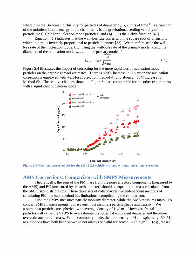
Figure S.4 illustrates the impact of correcting for the more rapid loss of nucleation mode particles on the organic aerosol estimates. There is ≈20% increase in OA when the nucleation correction is employed with wall-loss correction method #1 and about a ≈50% increase for Method #2. The relative changes shown in Figure S.4 are comparable for the other experiments with a significant nucleation mode.

Figure S.4 Wall-loss-corrected OA for the LEV2-2.1 vehicle with and without nucleation correction.

AMS Corrections: Comparison with SMPS Measurements Theoretically, the sum of the PM mass from the non-refractory components (measured by

the AMS) and BC (measured by the aethalometer) should be equal to the mass calculated from the SMPS size distributions. These three sets of data provide two independent methods of calculating PM, but each method has limitations, complicating the comparison.

First, the SMPS measures particle mobility diameter, while the AMS measures mass. To convert SMPS measurements to mass one must assume a particle shape and density. We assume that particles are spherical with average density of 1 g/cm3. However, fractal-like particles will cause the SMPS to overestimate the spherical equivalent diameter and therefore overestimate particle mass. While commonly made, the unit density [49] and sphericity [50, 51] assumptions have both been shown to not always be valid for aerosol with high EC (e.g., diesel

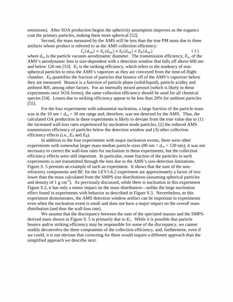
emissions). After SOA production begins the sphericity assumption improves as the organics coat the primary particles, making them more spherical [52].

Second, the mass measured by the AMS will be less than the true PM mass due to three artifacts whose product is referred to as the AMS collection efficiency: 𝐶𝑒(𝑑𝑣𝑎) = 𝐸𝐿(𝑑𝑣𝑎) × 𝐸𝑆(𝑑𝑣𝑎) × 𝐸𝐵(𝑑𝑣𝑎) ( 3 ) where dva is the particle vacuum aerodynamic diameter. The transmission efficiency, EL, of the AMS’s aerodynamic lens is size-dependent with a detection window that falls off above 600 nm and below 120 nm [53]. ES is the striking efficiency, which refers to the tendency of non-spherical particles to miss the AMS’s vaporizer as they are conveyed from the time-of-flight chamber. EB quantifies the fraction of particles that bounce off of the AMS’s vaporizer before they are measured. Bounce is a function of particle phase (solid/liquid), particle acidity and ambient RH, among other factors. For an internally mixed aerosol (which is likely in these experiments once SOA forms), the same collection efficiency should be used for all chemical species [54]. Losses due to striking efficiency appear to be less than 20% for ambient particles [55].

For the four experiments with substantial nucleation, a large fraction of the particle mass was in the 10 nm < dva < 30 nm range and, therefore, was not detected by the AMS. Thus, the calculated OA production in these experiments is likely to deviate from the true value due to (1) the increased wall-loss rates experienced by nucleation mode particles, (2) the reduced AMS transmission efficiency of particles below the detection window and (3) other collection efficiency effects (i.e., ES and EB).

In addition to the four experiments with major nucleation events, there were other experiments with somewhat larger mass median particle sizes (80 nm < dva < 120 nm); it was not necessary to correct the wall-loss rates for nucleation in these experiments, but the collection efficiency effects were still important. In particular, some fraction of the particles in such experiments is not transmitted through the lens due to the AMS’s size-detection limitations. Figure S. 5 presents an example of such an experiment. It shows that the sum of the non-refractory components and BC for the LEV1-6.2 experiment are approximately a factor of two lower than the mass calculated from the SMPS size distributions (assuming spherical particles and density of 1 g cm-3). As previously discussed, while there is nucleation in this experiment Figure S.2, it has only a minor impact on the mass distribution—unlike the large nucleation effect found in experiments with behavior as described in Figure S.3. Nevertheless, as this experiment demonstrates, the AMS detection window artifact can be important in experiments even when the nucleation event is small and does not have a major impact on the overall mass distribution (and thus the wall-loss rate).

We assume that the discrepancy between the sum of the speciated masses and the SMPS-derived mass shown in Figure S. 5 is primarily due to EL. While it is possible that particle bounce and/or striking efficiency may be responsible for some of the discrepancy, we cannot readily deconvolve the three components of the collection efficiency, and, furthermore, even if we could, it is not obvious that correcting for them would require a different approach than the simplified approach we describe next.

Figure S.5 Comparison of the sum of BC (measured by the aethalometer), organics, sulfate, nitrate and ammonium (measured by the AMS) against the total particle mass measured by the SMPS for the LEV1-6.2 experiment. Data are not wall-loss corrected.

For those experiments with the AMS+BC vs. SMPS discrepancy, we assume that the difference in mass has the same chemical composition as the speciated components. We then calculate a scaling factor, 𝐴𝑀𝑆𝑠.𝑓., that increases the sizes of the four colored wedges in Figure S. 5 proportionally such that their sum closes the gap with the SMPS measurement (dashed line). The scaling factor is

𝐴𝑀𝑆𝑠.𝑓. =𝐶𝑆𝑀𝑃𝑆 − 𝐶𝐵𝐶

𝐶𝑜𝑟𝑔 + 𝐶𝑆𝑂4 + 𝐶𝑁𝑂3 + 𝐶𝑁𝐻4 ( 4 )

where CSMPS is the total particle concentration measured by the SMPS, CBC is the black carbon concentration measured by the aethalometer, 𝐶𝑜𝑟𝑔, 𝐶𝑆𝑂4, 𝐶𝑁𝑂3, and 𝐶𝑁𝐻4 are the concentrations of organics, sulfate, nitrate and ammonium measured by the AMS. The values for AMSs.f. were calculated for each time step after nucleation, excluding the times when the aerosol passed through the thermodenuder, and then these values were averaged over the three hour UV exposure period. The AMSs.f. was used to scale the AMS data for the LEV1-5.2, LEV1-6.1, LEV1-6.2, LEV2-1.6, LEV2-2.1 and LEV2-4.2 experiments. In these experiments the average AMSs.f. ranged between 1.13 and 2.01, and the coefficient of variation within each experiment was between 7% and 18%. The AMSs.f. was not used to scale the data from other experiments either because the larger median particle size didn’t warrant it or because the AMSs.f. was too uncertain (i.e., the COV was greater than 20%).

0 0.5 1 1.5 2 2.50.0

2.0

4.0

6.0

8.0

10.0

12.0

14.0

16.0

18.0

time since lights on (h)

conc

entr

atio

n (µ

g/m

3 )

BCorgSO4NO3

NH4

SMPS

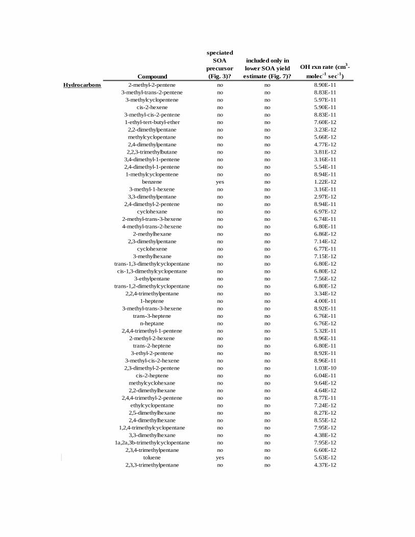
Table S.5 NMOGs as discussed in Figure 3, their OH reaction rates and the SOA yield cases in which they are included (Figure 7).

Compound

speciated SOA

precursor (Fig. 3)?

included only in lower SOA yield estimate (Fig. 7)?

OH rxn rate (cm3-molec-1 sec-1)

Hydrocarbons ethane no no 2.48E-13ethene no no 8.52E-12

propane no no 1.09E-12propene no no 2.63E-11

methylpropane no no 2.12E-12ethyne no no 8.15E-13

n-butane no no 2.36E-121,2-propadiene no no 9.82E-12trans-2-butene no no 6.40E-11

1-butene no no 3.14E-112-methyl-2-butene no no 8.69E-11

cis-2-butene no no 5.64E-112,2-dimethylpropane no no 6.69E-13

2-methylbutane no no 3.60E-121-propyne no no 7.14E-12

1,2-butadiene no no 2.60E-111,3-butadiene no no 6.66E-11

trans-2-pentene no no 6.70E-112-methylpropene no no 5.14E-11

1-pentene no no 3.14E-112-methyl-1-butene no no 6.10E-11

cis-2-pentene no no 6.50E-111-buten-3-yne no no 4.01E-11

2-butyne no no 2.73E-111-butyne no no 8.10E-12

1,3-butadiyne no no 1.82E-113-methyl-1-butene no no 2.86E-11

n-pentane no no 3.80E-122-methyl-1,3-butadiene no no 1.00E-103,3-dimethyl-1-butene no no 2.80E-11trans-1,3-pentadiene no no 1.60E-122,2-dimethylbutane no no 2.23E-12

cyclopentene no no 6.70E-114-methyl-1-pentene no no 3.02E-113-methyl-1-pentene no no 3.02E-11

cyclopentane no no 4.97E-122,3-dimethylbutane no no 5.78E-12

2,3-dimethyl-1-butene no no 5.38E-11methyl-tert-butyl-ether no no 2.26E-124-methyl-cis-2-pentene no no 5.88E-11

2-methylpentane no no 5.45E-124-methyl-trans-2-pentene no no 6.64E-11

3-methylpentane no no 5.73E-121-hexene no no 3.70E-11

2-methyl-1-pentene no no 5.40E-11n-hexane no no 6.97E+12

trans-3-hexene no no 6.62E-11cis-3-hexene no no 5.86E-11

trans-2-hexene no no 6.66E-11

Compound

speciated SOA

precursor (Fig. 3)?

included only in lower SOA yield estimate (Fig. 7)?

OH rxn rate (cm3-molec-1 sec-1)

Hydrocarbons 2-methyl-2-pentene no no 8.90E-113-methyl-trans-2-pentene no no 8.83E-11

3-methylcyclopentene no no 5.97E-11cis-2-hexene no no 5.90E-11

3-methyl-cis-2-pentene no no 8.83E-111-ethyl-tert-butyl-ether no no 7.60E-12

2,2-dimethylpentane no no 3.23E-12methylcyclopentane no no 5.66E-122,4-dimethylpentane no no 4.77E-122,2,3-trimethylbutane no no 3.81E-12

3,4-dimethyl-1-pentene no no 3.16E-112,4-dimethyl-1-pentene no no 5.54E-111-methylcyclopentene no no 8.94E-11

benzene yes no 1.22E-123-methyl-1-hexene no no 3.16E-113,3-dimethylpentane no no 2.97E-12

2,4-dimethyl-2-pentene no no 8.94E-11cyclohexane no no 6.97E-12

2-methyl-trans-3-hexene no no 6.74E-114-methyl-trans-2-hexene no no 6.80E-11

2-methylhexane no no 6.86E-122,3-dimethylpentane no no 7.14E-12

cyclohexene no no 6.77E-113-methylhexane no no 7.15E-12

trans-1,3-dimethylcyclopentane no no 6.80E-12cis-1,3-dimethylcyclopentane no no 6.80E-12

3-ethylpentane no no 7.56E-12trans-1,2-dimethylcyclopentane no no 6.80E-12

2,2,4-trimethylpentane no no 3.34E-121-heptene no no 4.00E-11

3-methyl-trans-3-hexene no no 8.92E-11trans-3-heptene no no 6.76E-11

n-heptane no no 6.76E-122,4,4-trimethyl-1-pentene no no 5.32E-11

2-methyl-2-hexene no no 8.96E-11trans-2-heptene no no 6.80E-11

3-ethyl-2-pentene no no 8.92E-113-methyl-cis-2-hexene no no 8.96E-112,3-dimethyl-2-pentene no no 1.03E-10

cis-2-heptene no no 6.04E-11methylcyclohexane no no 9.64E-122,2-dimethylhexane no no 4.64E-12

2,4,4-trimethyl-2-pentene no no 8.77E-11ethylcyclopentane no no 7.24E-12

2,5-dimethylhexane no no 8.27E-122,4-dimethylhexane no no 8.55E-12

1,2,4-trimethylcyclopentane no no 7.95E-123,3-dimethylhexane no no 4.38E-12

1a,2a,3b-trimethylcyclopentane no no 7.95E-122,3,4-trimethylpentane no no 6.60E-12

toluene yes no 5.63E-122,3,3-trimethylpentane no no 4.37E-12

Compound

speciated SOA

precursor (Fig. 3)?

included only in lower SOA yield estimate (Fig. 7)?

OH rxn rate (cm3-molec-1 sec-1)

Hydrocarbons 2,3-dimethylhexane no no 8.55E-122-methylheptane no no 4.77E-124-methylheptane no no 8.56E-12

3,4-dimethylhexane no no 8.84E-123-methylheptane no no 8.56E-12

cis-1,2-dimethylcyclohexane no no 1.19E-11trans-1,4-dimethylcyclohexane no no 1.19E-11

2,2,5-trimethylhexane yes no 6.05E-12trans-1-methyl-3-ethylcyclopentane no no 8.39E-12cis-1-methyl-3-ethylcyclopentane no no 8.39E-12

1-octene no no 3.30E-112,2,4-trimethylhexane yes no 6.33E-12

trans-4-octene no no 6.90E-11n-octane no no 8.11E-12

trans-2-octene no no 6.94E-11trans-1,3-dimethylcyclohexane no no 1.19E-11

2,4,4-trimethylhexane yes no 5.78E-12cis-2-octene no no 6.18E-11

2,3,5-trimethylhexane yes no 9.96E-122,4-dimethylheptane yes no 9.97E-12

cis-1,3-dimethylcyclohexane no no 1.19E-112,6-dimethylheptane yes no 9.68E-12

ethylcyclohexane no no 1.20E-113,5-dimethylheptane yes no 1.02E-11

ethylbenzene yes no 7.00E-121,3,5-trimethylcyclohexane yes no 1.35E-11

2,3-dimethylheptane yes no 9.97E-12m-xylene yes no 2.31E-11p-xylene yes no 1.43E-11

4-methyloctane yes no 9.97E-122-methyloctane yes no 9.69E-123-methyloctane yes no 9.97E-12

styrene yes no 5.80E-11o-xylene yes no 1.36E-11

2,2,4-trimethylheptane yes no 7.75E-121-methyl-4-ethylcyclohexane yes no 1.37E-11

2,2,5-trimethylheptane yes no 7.75E-121-nonene yes no 3.44E-11n-nonane yes no 9.70E-12

3,3-dimethyloctane yes no 7.21E-12(1-methylethyl)benzene yes no 6.90E-12

2,3-dimethyloctane yes no 1.14E-112,2-dimethyloctane yes no 7.47E-122,5-dimethyloctane yes no 1.14E-112,4-dimethyloctane yes no 1.14E-122,6-dimethyloctane yes no 1.14E-13n-propylbenzene yes no 5.80E-12

1-methyl-3-ethylbenzene yes no 1.39E-111-methyl-4-ethylbenzene yes no 7.44E-121,3,5-trimethylbenzene yes no 5.67E-11

2-methylnonane yes no 1.11E-111-methyl-2-ethylbenzene yes no 7.44E-12

Compound

speciated SOA

precursor (Fig. 3)?

included only in lower SOA yield estimate (Fig. 7)?

OH rxn rate (cm3-molec-1 sec-1)

Hydrocarbons 1,2,4-trimethylbenzene yes no 3.25E-11(2-methylpropyl)benzene yes no 8.71E-12(1-methylpropyl)benzene yes no 8.50E-12

n-decane yes no 1.10E-111-methyl-3-(1-methylethyl)benzene yes no 1.45E-11

1,2,3-trimethylbenzene yes no 3.27E-111-methyl-4-(1-methylethyl)benzene yes no 8.54E-12

indan yes no 8.28E-121-methyl-2-(1-methylethyl)benzene yes no 8.54E-12

1,3-diethylbenzene yes no 3.25E-111-methyl-3-n-propylbenzene yes no 1.52E-11

1,4-diethylbenzene yes no 3.25E-111-methyl-4-n-propylbenzene yes no 8.80E-121,3-dimethyl-5-ethylbenzene yes no 3.44E-11

1,2-diethylbenzene yes no 5.80E-121-methyl-2-n-propylbenzene yes no 8.80E-121,4-dimethyl-2-ethylbenzene yes no 1.69E-111,3-dimethyl-4-ethylbenzene yes no 1.76E-111,2-dimethyl-4-ethylbenzene yes no 1.69E-111,3-dimethyl-2-ethylbenzene yes no 1.76E-11

n-undecane yes no 1.25E-111,2-dimethyl-3-ethylbenzene yes no 1.69E-111,2,4,5-tetramethylbenzene yes no 3.25E-111,2,3,5-tetramethylbenzene yes no 4.31E-11

1-(dimethylethyl)-2-methylbenzene yes no 6.74E-125-methylindan yes no 1.79E-114-methylindan yes no 1.79E-11

1-ethyl-2-n-propylbenzene yes no 9.47E-122-methylindan yes no 9.42E-12

1,2,3,4-tetramethylbenzene yes no 2.05E-11n-pentylbenzene yes no 1.01E-11

1-methyl-2-n-butylbenzene yes no 1.02E-11naphthalene yes no 2.30E-11

1-(dimethylethyl)-3,5-dimethylbenzene yes no 3.01E-111,3-di-n-propylbenzene yes no 1.08E-11

n-dodecane yes no 1.32E-11

Carbonyls formaldehyde no no 9.37E-12acetaldehyde no no 1.50E-11

acrolein no no 2.58E-11acetone no no 1.70E-13

propionaldehyde no no 2.20E-11crotonaldehyde no no 3.62E-11methacrolein no no 2.90E-11

MEK no no 1.33E-12butyraldehyde no no 2.40E-11benzaldehyde yes no 1.20E-11valeraldehyde no no 2.74E-11

m-tolualdehyde yes no 1.70E-11hexanal no no 3.00E-11

Other unspeciated NMOG no yes 2.00E-11SVOC/IVOC yes yes 3.00E-11

Table S.6. Emission factors measured in the CVS and SOA production factors for all chamber experiments.

test dateCARB test

ID expt ID

model year

UC driving cycle

NMOG (g/kg)

CO (g/kg)NOx

(g/kg)CVS POA (mg/kg)

EC (mg/kg)

SOA, OH=5x106

(mg/kg)2/14/12 1032442 PreLEV-1.1 1987 Cold 8.82 209.46 8.79 54.1 35.9 26.92/10/12 1032440 PreLEV-2.1 Cold 34.98 332.34 19.64 136.3 44.4 108.42/13/12 1032444 PreLEV-2.2 Cold 31.41 328.25 19.48 102.4 29.2 89.61/31/12 1032303 PreLEV-3.2 Cold 5.62 72.07 8.16 57.8 2.4 46.72/1/12 1032389 PreLEV-3.3 Cold 5.36 73.14 8.34 48.7 3.1 70.22/8/12 1032426 PreLEV-3.4 Hot 2.68 49.56 5.44 0.5 2.4 n/a

5/26/10 1027859 LEV1-1.5 1996 Cold 2.35 19.83 4.44 3.4 0.8 10.11/17/12 1032302 LEV1-2.1 Cold 1.28 17.90 2.34 0.1 1.9 n/a1/18/12 1032304 LEV1-2.2 Cold 1.49 22.57 2.39 0.8 3.0 43.72/15/12 1032473 LEV1-2.3 Hot 0.23 9.97 1.25 4.1 4.0 22.31/25/12 1032346 LEV1-3.2 Cold 1.13 24.63 2.07 0.4 3.3 39.81/26/12 1032362 LEV1-3.4 Cold 1.20 28.36 2.30 0.2 1.4 56.12/6/12 1032393 LEV1-4.1 1999 Cold 0.95 45.32 3.63 2.3 4.0 35.26/3/10 1027904 LEV1-5.2 2000 Cold 1.61 14.77 2.05 26.1 3.5 35.6

5/28/10 1027881 LEV1-6.1 Cold 17.82 162.62 21.16 101.9 86.7 30.36/1/10 1027917 LEV1-6.2 Cold 15.02 157.54 20.16 106.2 122.2 131.46/2/10 1027918 LEV1-6.3 Cold 15.47 155.48 21.97 88.8 51.6 n/a

5/27/10 1027865 LEV2-1.2 Cold 0.60 17.94 0.40 4.6 12.0 35.86/9/10 1027967 LEV2-1.6 Cold 0.53 21.16 0.45 2.2 12.5 26.3

6/15/10 1028022 LEV2-2.1 2008 Cold 0.67 7.78 0.57 4.8 21.1 10.41/12/12 1032268 LEV2-3.1 Cold 0.42 7.12 0.30 0.0 0.0 8.81/13/12 1032283 LEV2-3.2 Cold 0.50 9.13 0.34 0.3 12.8 31.81/27/12 1032360 LEV2-3.3 Hot 0.08 2.10 0.16 -0.5 10.7 6.31/30/12 1032359 LEV2-3.4 Hot 0.20 1.24 0.23 0.0 13.6 1.66/10/10 1027971 LEV2-4.2 2010 Cold 0.40 6.33 0.08 2.4 33.2 17.41/23/12 1032342 LEV2-5.1 Cold 0.41 21.44 0.56 4.1 32.1 54.61/24/12 1032351 LEV2-5.2 Cold 0.51 14.97 0.63 1.3 35.2 24.91/19/12 1032309 LEV2-6.2 Cold 0.59 11.99 0.21 -0.4 2.4 4.31/20/12 1032321 LEV2-6.3 Cold 0.74 9.20 0.15 0.3 1.1 2.0

1998

LEV

I

1997

2003

1990Pre-

LEV 1988

2011

2011

LEV

II

2007

2008

Figure S.6. Log-log plots of individual NMOG species detected by the GC. Points above (below) the trendlines indicate species that were reduced less (more) than the majority of the other species. The lack of significant outliers suggests that the relatively small reduction in SOA production for newer LEV2 vehicles is due to unspeciated SOA precursors rather than those identified by the GC.