validation of high strain rate, multiaxial loads by
TRANSCRIPT

VALIDATION OF HIGH STRAIN RATE, MULTIAXIAL LOADS
USING AN IN-PLANE LOADER, DIGITAL IMAGE CORRELATION, AND FEA
by
Christopher Stroili
A thesis submitted in partial fulfillment
of the requirements for the degree
of
Master of Science
in
Mechanical Engineering
MONTANA STATE UNIVERSITY
Bozeman, Montana
November 2018

©COPYRIGHT
by
Christopher Stroili
2018
All Rights Reserved

ii
TABLE OF CONTENTS
1. INTRODUCTION ............................................................................................... 1
Motivation ............................................................................................................ 1
Elastic and Plastic Deformations ......................................................................... 2
Strain Rate Sensitive Constitutive Models .......................................................... 3
Materials Tested ............................................................................................. 3
Strain Rate Sensitive Plasticity (Viscoplastics) ............................................. 4
Work of Johnson-Cook .................................................................................. 6
Work of Zerilli and Armstrong..................................................................... 10
Mechanical Threshold Stress- Follansbee and Kocks ................................. 16
Multiaxial Loading at MSU ............................................................................... 24
Description and History of the Montana State In Plane Loader ........................ 24
Montana State University IPL ..................................................................... 26
Digital Image Correlation ............................................................................ 27
2. TESTING PROCEDURE .................................................................................. 29
Tensile Testing for Verification .......................................................................... 29
IPL Testing Procedure ........................................................................................ 37
3. ANALYSIS PROCEDURE ............................................................................... 43
Abaqus ............................................................................................................... 43
Background .................................................................................................. 43
Abaqus Model .............................................................................................. 43
4. POST PROCESSING DATA ............................................................................. 53
5. RESULTS AND DISCUSSION ........................................................................ 59
Strain Rate Sensitive Characterization of Materials .......................................... 59
Comparison of Results ....................................................................................... 60
IPL Sample 4 -304 Stainless Steel ............................................................... 67
Coupon 3- Multiaxial Case .......................................................................... 84
6. CONCLUSIONS ............................................................................................. 100
Future Work and Recommendations ................................................................ 101
7. REFERENCES ................................................................................................ 104

iii
TABLE OF CONTENTS CONTINUED
8. APPENDICES ................................................................................................. 108
APPENDIX A: MATLAB CURVE FITTING OF TENSILE DATA ........ 109
APPENDIX B: COMPARISON OF STRAIN DATA, FEA VS. DIC ....... 120

iv
LIST OF TABLES
Table Page
1. Comparison of various material testing rates.................................................... 6
2. Johnson-Cook constants for a variety of metals, as determined
by the researchers in 1983................................................................................. 9
3. Comparison of Zerilli Armstrong model ((Eq. (22)), Johnson
Cook Model ((Eq(1)), and Johnson Cook experimental. ................................ 13
4. State variables for MTS UHARD subroutine as defined by Van
Rensburg and Koks. ....................................................................................... 22
5. Elastic Modulus for 304 Stainless Steel, determined by tensile
testing. ............................................................................................................. 30
6. Values used to validate Johnson-Cook coefficients. ....................................... 31
7. Results from elastic and plastic region curve fits. .......................................... 35
8. Steel coupon test matrix for the IPL. D1 is notch width, D2 is
the reduced thickness at the coupons midgage. Dimensions in
inches IAW IPL input parameters. .................................................................. 42
9. Johnson Cook constants used by A. Maurel-Pantel et al. for
304L stainless steel, showing similar properties to 304
stainless. .......................................................................................................... 42
10. Percent differences between the maximum principal strain in
the FEA and DIC results along the center of the gage section.
t=2s .................................................................................................................. 70
11. Percent differences between the maximum principal strain in
the FEA and DIC results along the center of the gage section. t
=3.4s ................................................................................................................ 74
12. Percent differences between the maximum principal strain in
the FEA and DIC results along the center of the gage section. t
=4s. .................................................................................................................. 77
13. Percent differences between the maximum principal strain in
the FEA and DIC results along the center of the gage section. t
=4.8s. ............................................................................................................... 81

v
LIST OF TABLES CONTINUED
Table Page
14. Percent differences between the maximum principal strain in
the FEA and DIC results along the center of the gage section. t
=4.8s. ............................................................................................................... 88
15. Percent differences between the maximum principal strain in
the FEA and DIC results along the center of the gage section. t
=5.0s. ............................................................................................................... 92
16. Percent differences between the maximum principal strain in
the FEA and DIC results along the center of the gage section. t
=15.8s. ............................................................................................................. 96

vi
LIST OF FIGURES
Figure Page
1. Stress/Strain curve with linear elastic region highlighted in red
box..................................................................................................................... 2
2. Studying the effects of ballistic impacts on tank armor during
World War II. .................................................................................................... 4
3. Plot created by U.F. Kocks illustrating temperature and strain
rate dependence in aluminum. .......................................................................... 5
4. Johnson and Cook's comparison of their computational model
to cylinder impact tests. .................................................................................... 8
5. G.I. Taylor developed the Taylor test to explore strain
hardening in his 1947 paper. ............................................................................11
6. Abaqus flow chart used by Bonorchis to illustrate VUMAT
solver. .............................................................................................................. 14
7. An example of results comparing the Abaqus prepackaged
Johnson Cook Model (a), a custom Johnson-Cook VUMAT (b),
and a custom Zerilli-Armstrong VUMAT (c). ................................................ 15
8. Strain hardening curves for OFHC copper using MTS equation. ................... 16
9. Skeleton code for Abaqus UHARD model. .................................................... 20
10. Flowchart for Van Rensburg and Koks UHARD subroutine for
MTS constitutive model. ................................................................................. 22
11. Van Rensberg and Kok's results comparing Johnson-Cook
model with their MTS UHARD code. Material simulated was
OFHC copper. ................................................................................................ 23
12. Van Rensberg and Kok's results with their MTS UHARD code.
Material simulated was OFHC copper. ........................................................... 23
13. Original In-Plane Loader designed by the Navy Research Labs. ................... 25
14. Combined loading conditions that can be applied by the NRL
IPL................................................................................................................... 26

vii
LIST OF FIGURES CONTINUED
Figure Page
15. Schematic of DIC camera set-up as used with the In-Plane
Loader. ............................................................................................................ 27
16. Plot of Abaqus simuluations illustrating the Johnson Cook
strain rate sensitive plastic deformation in 304L stainless steel.
An IPL test falls between 0.07s-1 and 0.3s-1. ................................................... 29
17. Plot of the elastic modulus curve fit and test data for a 304
stainless steel coupon. ..................................................................................... 31
18. Plot comparing test data with elastic modulus slope, used to
determine proportional limit. .......................................................................... 33
19. Plot of calculated Stress = (E x Strain) - test data stress value,
plotted against stress. This is used to determine when the
material has yielded. ....................................................................................... 34
20. MATLAB Curve fitting app, A is filled with each tests
respective value, B and n are solved for. ........................................................ 35
21. Plot of the MATLAB generated curve fit overlaid onto data
from tensile tests. ............................................................................................ 36
22. IPL coupon geometry for stainless steel. Drawing dimensions
in inches. ......................................................................................................... 36
23. GOM designed camera set up used for IPL testing; cameras are
mounted at a set distance from one another. Lighting elements
can be adjusted for optimum position. ............................................................ 39
24. Desirable stochastic spray pattern on 304 stainless steel. ............................... 40
25. IPL Coupon geometry as modeled in Abaqus/CAE 2017
(dimensions in millimeters) ............................................................................ 44
26. Initial Johnson-Cook material parameters as input into
Abaqus/CAE ................................................................................................... 45
27. Meshed IPL sample geometry in Abaqus. ...................................................... 45

viii
LIST OF FIGURES CONTINUED
Figure Page
28. Abaqus dialog box showing parameters used in the implicit
dynamic step. .................................................................................................. 47
29. Boundary conditions applied to the bottom surface of the
coupon. ............................................................................................................ 48
30. Depiction of reference point (in red circle) location on the 3D
solid model. ..................................................................................................... 49
31. A Coupling Constraint is used to couple displacements of a
control point (RP) to a surface (top surface of coupon).
Displacement of the surface is dictated by the reference point
in all directions. ............................................................................................... 50
32. Table of time and displacements, in millimeters (displacement)
or radians (rotation) as exported from Aramis and imported
into Abaqus. .................................................................................................... 51
33. Boundary condition dialogue box showing the X displacement
applied to the reference point. This is repeated for Y and
rotation displacements (U2, UR3). ................................................................. 52
34. Aramis contour surface showing ε22 for a stainless steel
coupon, facet grid is shown. Note the hole in the bottom left
corner............................................................................................................... 55
35. Abaqus contour surface showing ε22 for a stainless st .................................... 56
36. Aramis cross sectional path on an IPL coupon. .............................................. 57
37. Highlighted Abaqus cross sectional path. ....................................................... 57
38. Deformed shape of a center section in Aramis. ε22. ........................................ 58
39. Deformed shape of a center section in Abaqus. ε22......................................... 58
40. Samples showing striations on the right half of the coupons
indicating severe grip slip. Rotation (top) and Vertical (bottom) ................... 60
41. Plot of Abaqus simulations illustrating the Johnson Cook strain
rate sensitive plastic deformation in 304L stainless steel. An
IPL test falls between 0.07 s-1 and 0.3 s-1. ....................................................... 61

ix
LIST OF FIGURES CONTINUED
Figure Page
42. Plot comparing the J-C model determined in Table 4 with
experimental tensile data................................................................................. 62
43. Plot of ε11 along center of an IPL coupon 4.4 seconds into a
test. .................................................................................................................. 63
44. Plot of ε22 along center of an IPL coupon, 4.4 seconds into a
test. .................................................................................................................. 64
45. of εP1 (maximum principal strain) along center of an IPL
coupon, 4.4 seconds into a test........................................................................ 65
46. 2mm into coupons gage section. (x = 2mm, y = 0mm). ................................. 65
47. Plot of maximum principal strain for FEA and DIC strain
results, appx. 2 mm into a coupon .................................................................. 66
48. Plot of maximum principal strain for FEA and DIC strain
results, appx. 2 mm into a coupon. ................................................................. 67
49. Plot of maximum principal strain for FEA and DIC strain
results, appx. 2 mm into a coupon. ................................................................. 68
50. Comparison of strain fields at 2 seconds, coupon 4, ε22.................................. 69
51. Cross sectional strain at the center of sample 5 at 2.6s, εP1 ............................ 71
52. Comparison of strain fields at 3.4 seconds, coupon 4, εP1 (L:
FEA, R: DIC) .................................................................................................. 72
53. Cross sectional strain at the center of sample 4 at t=3.4s, εp1 ......................... 73
54. Plot relating εP1 from the FEA model and experimental to the
Johnson Cook curve fit. At 3.4 seconds, 1.94 mm into the gage
section. Plot illustrates expected stress value at measured
strain. ............................................................................................................... 75
55. Comparison of strain fields at 4.0 seconds, coupon 4, εP1 (L:
FEA, R:DIC) ................................................................................................. 76
56. Cross sectional strain at the center of Coupon 4 at t =4s, εP1 ......................... 76

x
LIST OF FIGURES CONTINUED
Figure Page
57. Plot relating εP1 from the FEA model and experimental to the
Johnson Cook curve fit. At 4 seconds, 2mm into the gage
section. ............................................................................................................ 78
58. Comparison of strain fields at 4.8 seconds, coupon 4, εP1 (L:
FEA, R:DIC) .................................................................................................. 79
59. Cross sectional strain at the center of Coupon 4 at t =4.8s, εP1. ...................... 80
60. Plot relating εP1 from the FEA model and experimental to the
Johnson Cook curve fit. At 4.8 seconds, appx. 2mm into the
gage section. .................................................................................................... 82
61. Plot comparing strain in the ε22 direction against -2*(ε11). t =
2s. .................................................................................................................... 83
62. Plot comparing strain in the ε22 direction against -2*(ε11). t =
3.4s. ................................................................................................................. 83
63. Plot comparing strain in the ε22 direction against -2*(ε11). t =
4.0s. ................................................................................................................. 84
64. Plot comparing strain in the ε22 direction against -2*(ε11). t =
4.8s. ................................................................................................................. 85
65. Comparison of strain fields at 2.4 seconds, coupon 3, εP1 (L:
FEA, R: DIC) .................................................................................................. 86
66. Cross sectional strain at the center of coupon 3, at t = 2.6s, εP1 ..................... 87
67. Plot relating εP1 from the FEA model and experimental to the
Johnson Cook curve fit. At 2.4 seconds, in the center of the
gage section. .................................................................................................... 89
68. Comparison of strain fields at 5 seconds, coupon 3, εP1 (L:
FEA, R: DIC) .................................................................................................. 90
69. Cross sectional strain at the center of sample 3 at t =5.0 s, εP1 ....................... 91
70. Plot relating εP1 from the FEA model and experimental to the
Johnson Cook curve fit. At 5 seconds, 2 mm into the gage
section. ............................................................................................................ 93

xi
LIST OF FIGURES CONTINUED
Figure Page
71. Comparison of strain fields at 4.8 seconds, coupon 7, ε12 (L:
FEA, R: DIC) .................................................................................................. 94
72. Plot relating εP1 from the FEA model and experimental to the
Johnson Cook curve fit. At 5 seconds, 2 mm into the gage
section ............................................................................................................. 95
73. Plot comparing strain in the ε22 direction against -2*(ε11). t =
2.4s. ................................................................................................................. 97
74. Plot comparing strain in the ε22 direction against -2*(ε11). t =
5s. .................................................................................................................... 98
75. Plot comparing strain in the ε22 direction against -2*(ε11). t =
15.8s. ............................................................................................................... 98
76. IPL stage report generated by Aramis for sample 5, 5s into the
test. Note moment ZZ. .................................................................................. 102

xii
ABSTRACT
Montana State University’s In-Plane Loader (IPL) is a machine designed to test
for mechanical properties at multi-axial states of stress and strain by in-plane translation
and rotation. Historically the machine has been used to characterize composite lay-ups,
where applying multi-axial loads can better describe anisotropic materials. The IPL
testing machine uses Digital Image Correlation (DIC) software and a stereoscopic camera
system to measure strains on the surface of the test coupon by tracking a stochastic
pattern applied to the gage section.
The focus of this work was to test the capabilities beyond quasi-static composites
testing, specifically looking to explore the feasibility of testing plastics and metals at
strain rates from 100 to 103 s-1. This work explored the speed and loading capabilities of
the IPL and determined a suitable coupon geometry which balances gage section area
with material strength. 304 Stainless Steel was tested both on the IPL and in uniaxial
tension. Experimental tensile test data was fit to a Johnson Cook strain rate sensitive
constitutive model. This constitutive equation was then used with an implicit dynamic
finite element analysis (FEA) model. To study the validity of high rate testing of steel in
the IPL, strain from the DIC experimental data was compared with the FEA results.
While the strains predicted by the FEA model varied from experimental results, a better
understanding of the IPL capabilities has been achieved. Moving forward, a series of
recommendations have been made so that high strain rate multi-axial testing of metals
can be implemented with more robust constitutive models.

1
INTRODUCTION
Motivation
In order to classify a materials behavior their material properties must be
determined. Tests for intrinsic material properties such as elastic modulus (E), shear
modulus (G), and Poisson’s ratio (𝜈) are carried out in pure tension or shear as to eliminate
off axis loading. However, when parts are designed for use, rarely do loads act in pure
tension or shear on the component. Multiaxial systems are utilized to experientially study
non-ideal load cases. The In-Plane Loader (IPL), combined with Aramis Digital Image
Correlation software (DIC) allows for a user to study the effects of a complex loading path,
while outputting force, displacement, and strain data, with minimal post processing.
In the interest of developing a better understanding of materials experiencing multi-
axial loads under elevated strain rates. The objectives of this research project are:
1. Validate the in-plane loaders ability to characterize behavior of strain rate
sensitive materials under multiaxial loading.
2. Develop a method to compare data collected by the In-Plane Loader and
digital image correlation with results obtained using finite element analysis
software.
3. Provide input for the next iteration of the In-Plane Loader.

2
Elastic and Plastic Deformations
When designing parts and assemblies, it is desirable to stay within materials elastic
limits. Within a material’s elastic regime, it’s stress and strain curve behaves in a
predictable, linear manner as seen in Figure 1.
Figure 1. Stress/Strain curve with linear elastic region highlighted in red box.1
For an isotropic material, under a uniaxial load the behavior is like a linear spring.
This relationship is shown below (eqn. 1) in the tensor notation form.
𝜎𝑖𝑗 = 𝐶𝑖𝑗𝑘𝑙𝜖𝑘𝑙 (1)
Elastic deformation does not involve the breaking of atomic or chemical bonds,
but rather the stretching of the bonds [2]. Strain in the elastic regime is recovered when the
1 1. Dowling, N.E., Mechanical Behavior of Materials. Fourth ed. 2013, Upper Saddle River, NJ:
Pearson. 936.

3
applied load is removed. Unlike plasticity or creep, this deformation is independent of
loading rates or time [1].
When a material is placed under a load which exceeds its elastic limit, or yield
stress, an inelastic deformation occurs, causing a permanent change in atomic configuration
[2]. At this point a portion of the strain will remain in the material once the load is removed,
typically this plastic strain is time independent, however certain materials will exhibit a
time dependence [3]. In Mechanical Behavior of Materials, Dowling states that; “inelastic
deformation that occurs nearly instantaneously as the stress is applied is known as plastic
deformation”. This permanent deformation is caused by shear stress induced by the motion
of dislocations in the material. This is described as an incremental process as atomic bonds
are not broken simultaneously, but rather progress through the material [1].
Strain Rate Sensitive Constitutive Models
Materials Tested
The material chosen for this study was 304 Stainless Steel. This was chosen as 304
SS can represent a wider variety of materials with interesting strain rate sensitive
properties. The focus on stainless steel in this thesis was initially due to its strain rate
sensitivity, to explore the IPL’s ability to characterize strain rate sensitive multi-axial
loading. Adjustments to the materials geometries were made as testing progressed due to
discovering limitations in the IPL’s gripping ability. Historically at Montana State
University composite coupons were given a single notch to generate asymmetric strain
fields. The high elastic modulus of stainless steel used in this study led to a double notch
being used.

4
Strain Rate Sensitive Plasticity (Viscoplastics)
Many plastics and metals exhibit work hardening or a change in the stress/strain
slope, 𝑑𝜎
𝑑𝜖, when experiencing plastic deformation [3]. Historically understanding of high
strain rate plastic deformation behavior was driven by ballistic research. An early study of
the effectiveness of tank armor is show in Figure 2.
Figure 2. Studying the effects of ballistic impacts on tank armor during World War II.2
Furthermore, other relationships exist for work hardening. As temperature increases
material softening will occur, as strain rate increases stiffening occurs [4]. These high
temperature and strain rate conditions are both present in high speed impacts. This
phenomenon is also highly dependent on the materials crystal structure. In 1929 F.H.
Norton studied material flow rates at elevated temperatures, writing “It is only within a
relatively few years that the importance of the time element in determining the useful
2 https://www.snafu-solomon.com/2017/12/m4a3e2-jumbo-out-armored-tiger-1s.html
5
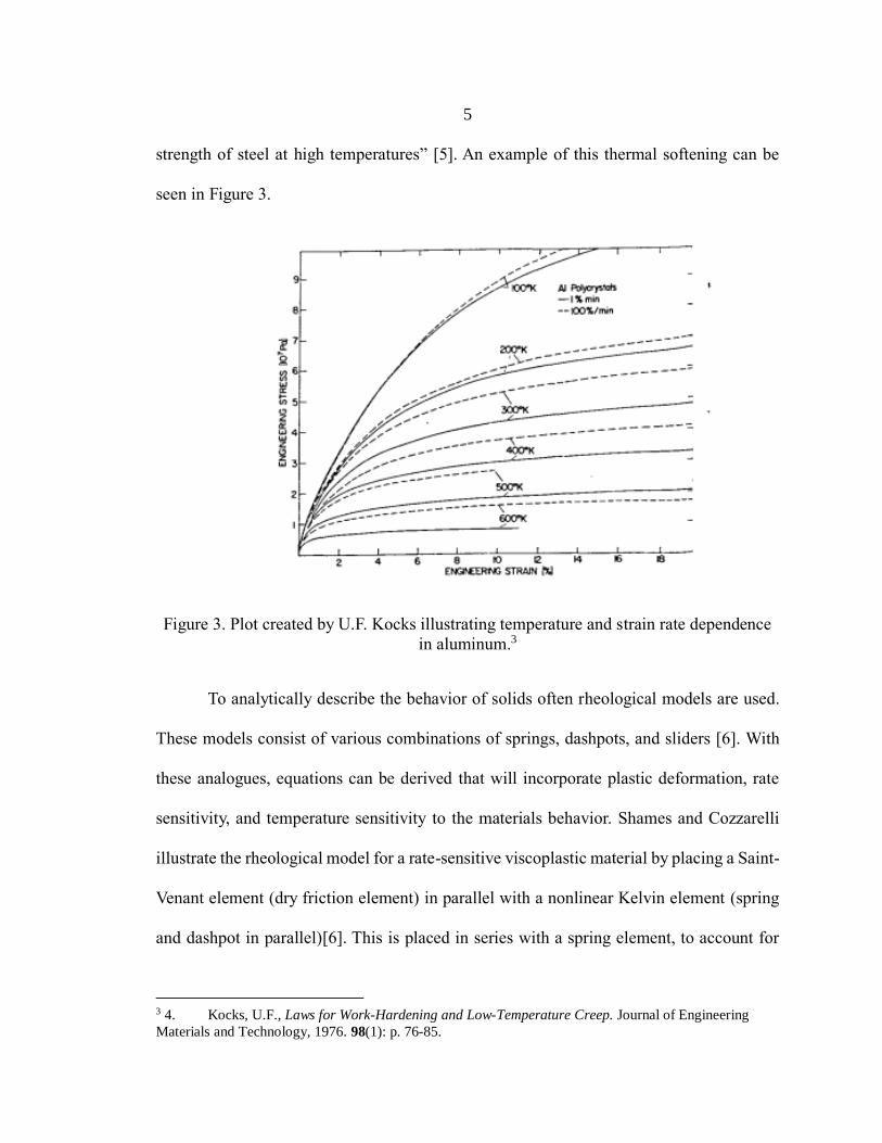
strength of steel at high temperatures” [5]. An example of this thermal softening can be
seen in Figure 3.
Figure 3. Plot created by U.F. Kocks illustrating temperature and strain rate dependence
in aluminum.3
To analytically describe the behavior of solids often rheological models are used.
These models consist of various combinations of springs, dashpots, and sliders [6]. With
these analogues, equations can be derived that will incorporate plastic deformation, rate
sensitivity, and temperature sensitivity to the materials behavior. Shames and Cozzarelli
illustrate the rheological model for a rate-sensitive viscoplastic material by placing a Saint-
Venant element (dry friction element) in parallel with a nonlinear Kelvin element (spring
and dashpot in parallel)[6]. This is placed in series with a spring element, to account for
3 4. Kocks, U.F., Laws for Work-Hardening and Low-Temperature Creep. Journal of Engineering
Materials and Technology, 1976. 98(1): p. 76-85.

6
the elastic deformation in the material. The authors show that the Saint-Venant element
forces these constraints. While useful, experimental testing and validation can provide a
more accurate material model.
The IPL is unique in that it is capable of testing materials at speeds between quasi-
static and ballistic impacts. An area which has not been covered in depth historically. Table
1 contains a range of strain rates, and where the IPL capabilities lie.
Table 1. Comparison of various material testing rates.
Test Type Test Rate
Quasi-Static 10-4 to 10-3 s-1
In-Plane Loader 10-2 to 100 s-1
Car Accident/Ballistic Impact 102 to 103 s-1
Explosives 103 to 105 s-1
Work of Johnson-Cook
Published in 1985, Gordon R. Johnson of Honeywell Inc. Defense Systems
Division, and William H. Cook of the Air Force Armament Laboratory, modeled the high
strain rate and high temperature behavior of a variety of metals. Johnson and Cook
highlight that under dynamic loading (impacts, explosions, and metal forming operations)
high strain rates events additionally exhibit high temperatures and large strains [7]. The
researchers tested from quasi static speeds up to high strain rates up to 650 s-1 in dynamic
impacts. Johnson and Cook studied the effects of strain rate and temperature on oxygen-

7
free high thermal conductivity (OHFC) Copper, Armco Iron, 4340 steel, and nine other
metals. For von Mises tensile flow stress, Johnson and Cook arrived at the analytic
expression in Equation 3.
𝜎 = [𝐴 + 𝐵𝜖𝑛][1 + 𝐶𝑙𝑛𝜖̇∗][1 − 𝑇∗𝑚] (2)
Here A is the materials yield stress; B is the strain-hardening constant (in units of
stress). Strain is ε, the strain hardening exponent is n, and the strain rate constant is C.
Additionally, 𝜖̇∗ =�̇�
�̇�0 is a dimensionless plastic strain rate, a ratio where ε̇0 is an
experimentally determined reference strain rate (typically 1.0 s-1), and ε̇ is the plastic strain
rate. 𝑇∗ is the homologous temperature defined as 𝑇−𝑇0
𝑇𝑚−𝑇0, where T is testing temperature,
T0 is the reference temperature, and Tm is the materials melting temperature.
In Equation 2, the terms in the second and third terms are used to introduce strain
rate and temperature dependence, respectively, to the materials stress vs. strain relationship.
Johnson and Cook preformed quasi-static tensile tests, biaxial torsion/tension tests, and
Hopkinson bar tests to determine A, B, n, C, and m.
8
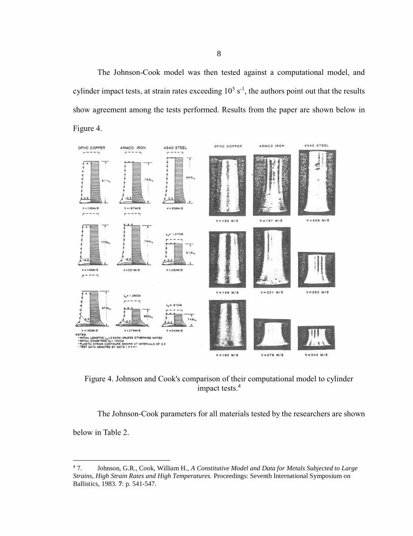
The Johnson-Cook model was then tested against a computational model, and
cylinder impact tests, at strain rates exceeding 105 s-1, the authors point out that the results
show agreement among the tests performed. Results from the paper are shown below in
Figure 4.
Figure 4. Johnson and Cook's comparison of their computational model to cylinder
impact tests.4
The Johnson-Cook parameters for all materials tested by the researchers are shown
below in Table 2.
4 7. Johnson, G.R., Cook, William H., A Constitutive Model and Data for Metals Subjected to Large
Strains, High Strain Rates and High Temperatures. Proceedings: Seventh International Symposium on
Ballistics, 1983. 7: p. 541-547.

9
Table 2. Johnson-Cook constants for a variety of metals, as determined by the researchers
in 1983.5
Using their equation for flow stress, Johnson and Cook conducted further research
to determine the strain to fracture of the same materials. This research will not study the
fracture behavior in depth, but it is worth noting that even in 1985 the authors mention their
interest in studying complicated loading paths, such as the multi-axial loads produced by
the IPL. Equation 3 is defined by the paper as strain to fracture
𝜖𝑓 = [𝐷1 + 𝐷2 exp(𝐷3𝜎∗)][1 + 𝐷4 ln 𝜖̇∗][1 + 𝐷5𝑇∗] (3)
While this research paper will not cover fracture mechanics at high strain rates, it
should be noted that this should be considered when further exploring future work using
the IPL.
5 7. Ibid.

10
Work of Zerilli and Armstrong
Frank J. Zerilli and Ronald W. Armstrong’s 1987 paper makes an attempt to offer
an improved version of a strain rate and temperature sensitive constitutive relation [8]. The
authors note that the flow stress of two of the materials Johnson and Cook tested: OHFC
copper, and Armco iron, show different dependencies on strain rate and temperature.
Noting that the OFHC copper shows a much higher strain dependence than the Armco iron.
Zerilli and Armstrong explore the idea of dislocation mechanics to better describe
constitutive relationships. Their first issue with existing theories is that cylinder impacts,
which are commonly used in high strain rate testing, do not provide a detailed description
of a materials strength. Dating back to 1947, a Taylor test shown in Figure 5, is sufficient
in predicting the ratio of final length to initial length based on a projectiles kinetic energy
[9].

11
This test, however it does not accurately work to model the shape of the deformed
projectile. At the time, the authors saw a weakness in computer codes as they relied heavily
on numerical fits, and they could not rely on these codes for predictions outside of existing
data.
Figure 5. G.I. Taylor developed the Taylor test to explore strain hardening in his 1947
paper.6
The focus of the 1987 paper was improving strain-rate and temperature sensitive
plasticity models exploring the notion that grain size of a material hugely influences
strength and ductility. The researchers point to drastically different results between
Johnson-Cook and Wilkins-Guinan constitutive models when studying copper impact tests
with computer simulations. They introduce the idea of using a model based on grain size,
accumulation of dislocations, and generation of dislocations by thermal activation energy.
Furthermore, the authors discuss the differences in strain rate and temperature dependence
for face centered cubic metals (FCC), and body centered cubic metals (BCC). For BCC
metals, the thermal activation is independent of plastic strain in the material, whereas for
an FCC, the thermal activation is observed to be highly dependent on plastic strain. Zerilli
6 9. Taylor, G., The Use of Flat-Ended Projectiles for Determining Dynamic Yield Stress. I.
Theoretical Considerations. Proceedings of the Royal Society of London. Series A, Mathematical and
Physical Sciences (1934-1990), 1948. 194(1038): p. 289-299.

12
and Armstrong arrived at two constitutive equations. Equation 4 gives stress for an FCC
metal, and Equation 5 gives stress for a BCC metal.
𝜎 = ∆𝜎𝐺′ + 𝑐2𝜖1 2⁄ exp[−𝑐3𝑇 + 𝑐4𝑇𝑙𝑛(𝜖̇)] + 𝑘𝑙−1 2⁄ (4)
𝜎 = ∆𝜎𝐺′ + 𝑐1 exp[−𝑐3𝑇 + 𝑐4𝑇𝑙𝑛(𝜖̇)] + 𝑐5𝜖𝑛 + 𝑘𝑙−1 2⁄ (5)
Where c1, c2, and c5 are units of stress (MPa), c3 and c4 are units of T-1 (K-1), n is
unitless, and k is in units of stress x length1/2 (MPa mm1/2). ∆𝜎𝐺′ in both equations is added
to account for dislocation density. When comparing experimental cylinder impact results
of the Zerelli Armstrong model with the Johnson and Cook’s model OFHC copper, it was
seen that the Johnson Cook model in Equation 2 did not predict large or small strains well
[8]. The Zerilli Armstrong model, however appeared to better agree with experimental
results. The results for the Zerilli Armstrong model applied to Armco iron did show a
noticeable difference when comparing impact test simulations. Their model predicted too
soft a material at large strains (as Johnson Cook does), but predicts a harder material at
small strains, where Johnson Cook has been observed to predict a soft material.

13
Table 3. Comparison of Zerilli Armstrong model (Eq. (22), Johnson Cook Model (Eq(1),
and Johnson Cook experimental.7
Abaqus Implementation of Zerilli Armstrong model
A Zerilli-Armstrong plasticity model was developed for Abaqus CAE by Dean
Bonorchis at the University of Cape down in his 2003 dissertation [10]. Bonorchis
programmed a VUMAT custom plasticity model to implement Zerilli Armstrong for BCC
and FCC materials. A VUMAT is a custom, user created material using an Abaqus explicit
dynamic simulation, as opposed to an implicit dynamic UMAT material. The Abaqus
explicit dynamic analysis module is computationally efficient for analyzing large models
7 8. Zerilli, F.J. and R.W. Armstrong, Dislocation‐mechanics‐based constitutive relations for material
dynamics calculations. Journal of Applied Physics, 1987. 61(5): p. 1816-1825.

14
[11]. The develop of Abaqus Dassault lists the advantages of this method in their
documentation, including its usefulness in simulation high-speed dynamic events such as
sheet metal forming[11]. Attempts were made to reproduce IPL tests with a Johnson-Cook
based simulation of 304 stainless steel, however difficulties with wave speed in the material
produced errors. A sample of the authors VUMAT process flowchart is shown below in
Figure 6.
Figure 6. Abaqus flow chart used by Bonorchis to illustrate VUMAT solver.8
8 10. Bonorchis, D., Implementation of Material models for High Strain Rate Applications as User-
subroutines in Abaqus/Explicit, in Mechanical Engineering. 2003, University of Cape Town. p. 229.

15
Bonorchis ran simple single element tests in various loading conditions using
Abaqus to verify the accuracy of his custom materials. To solve the constitutive equations
at each step, Bonorchis used a bisection and Newton methods in his solvers, however there
is only a brief description of these, and the work does not go into detail as to how the
equations were discretized. Once verification was complete, the author reproduced Taylor
impact tests to verify his VUMATs with experimental results of OFHC copper and Armco
iron, using the same methodology is Johnson and Cook, and Zerilli and Armstrong: by
comparing shape of slugs after the impact. A sample of his results are show below in Figure
7.
Figure 7. An example of results comparing the Abaqus prepackaged Johnson Cook Model
(a), a custom Johnson-Cook VUMAT (b), and a custom Zerilli-Armstrong VUMAT (c).9
9 10. Ibid.

16
Mechanical Threshold Stress- Follansbee and Kocks
P. S. Follansbee and U.F. Kocks developed the Mechanical Threshold Stress (MTS)
model at Los Alamos National Laboratory in 1986, building on their previous work into
strain rate sensitive of FCC metals [12]. The main property, the mechanical threshold stress,
is a materials flow stress at 0 K. Flow stress is the stress required to maintain plastic
deformation of a material, found between the materials yield stress and ultimate strength
MTS itself is a theoretical value. Figure 8 shows a plot of the stress and strain of OFHC
copper using mechanical threshold stress equation at varying rates.
Figure 8. Strain hardening curves for OFHC copper using MTS equation.10
10 12. Follansbee, P.S. and U.F. Kocks, A constitutive description of the deformation of copper based on
the use of the mechanical threshold stress as an internal state variable. Acta Metallurgica, 1988. 36(1): p.
81-93.

17
Like Zerilli and Armstrong’s work, the MTS model is based off of a materials
thermal activation energy and density of dislocations in the metal. The authors pointed to
a need for a single strain rate and temperature sensitive constitutive model that would also
behave predictably at low strain rates. Previous work at the time had not been utilized for
strain rates above ε̇ =103 s-1. This is important as the researchers note that strain rate
sensitivity can increase drastically above this value. Copper was chosen as the material of
interest as mechanical threshold stress data up to rates of ε̇ = 104 s-1 allows for the study
into strain rates at level where the material becomes increasing strain rate sensitive.
Mechanical threshold stress is defined by Equation 6 as;
�̂� = �̂�𝑎 + 𝑠(𝜖̇, 𝑇)�̂�𝑙 (6)
Where �̂�𝑎 accounts for rate independent effects, associated with grain boundaries
or long-range barriers. The second term is a scaling function contains rate dependency
associated with short-range obstacles. These are known respectively as the thermal and
athermal components of the equation[13]. An Arrhenius equation, Equation 7, is used to
account for a rate dependence on temperature [9].
𝜖̇ = 𝜖0̇ exp [
∆𝐺(𝜎𝑡 �̂�𝑡⁄ )
𝑘𝑇] (7)
Here ε̇0 is a constant value, and k is the Boltzman constant (1.38 x 10⁻²³ J-K-1 ), and
ΔG is the Gibb’s free energy in Equation 8 which is equal to
∆𝐺 = 𝑔0𝜇𝑏3 [1 − (
𝜎𝑡
𝜎�̂�)
𝑝
]𝑞
(8)

18
With g0 being a normalized activation energy, μ is the materials shear modulus b is
the magnitude of the Burger’s vector, p and q are constants, which are used to characterize
the shape of the obstacle profile, where 0 ≤ p ≤ 1, and 1 ≤ q ≤ 2 [12].
The authors combine these equations to arrive at the general expression for MTS in
Equation 9.
𝜎 = �̂�𝑎 + (�̂� − �̂�𝑎) {1 − [𝑘𝑇𝑙𝑛(𝜖0̇ 𝜖̇⁄ )
𝑔0𝜇𝑏3]
1𝑞
}
1𝑝
(9)
Follansbee and Kocks also discuss the strain hardening rate of an FCC metal, 𝜃 =
𝑑𝜎/𝑑𝜖, using the relation in Equation 10.
𝜃 = 𝜃0 − 𝜃𝑡(𝑇, 𝜖̇, �̂�) (10)
Where 𝜃0 is hardening by dislocation accumulation and is assumed constant. and
𝜃𝑡 is the dynamic recovery rate.
The researchers show that their model is capable of modelling changing strain rates
accurately, a feature that would be helpful when modeling a multi-axial in-plane loading
test of an FCC metal in the current in plane loader. They were successful in modelling
tensile tests of OFHC copper at strain rates from 10-4 s-1 to 104s-1 . It is noted that above
strain rates of 105 s-1 the model shows unrealistic perfect plasticity stress-strain behavior in
materials [12]. These strain rates are beyond those focus on in this IPL study.
An Abaqus user-hardening regimen was written by G.J. Jansen Van Rensburg and
S. Kok. This is a valuable tool to implement the MTS model in Abaqus. In their paper, the
researchers also used strain data of OFHC copper. Van Rensburg and Kok reduce the MTS
equation into smaller forms for simplified implementation as a UHARD and Fortran code
19
[13]. The thermal portion of the equation for MTS are further reduced by noting there are
two thermal components to the equation, arriving at Equation 11.
𝜎𝑦
𝜇=
�̂�𝑎
𝜇+ 𝑆𝑖(𝜖̇, 𝑇)
�̂�𝑖
𝜇0 + 𝑆𝜖(𝜖̇, 𝑇)
�̂�𝜖
𝜇0 (11)
Here, �̂�𝑖 is the non-evolving thermal portion of yield stress, �̂�𝜖 is used to account
for interaction with mobile dislocations and is the changing component of the equation. 𝜇0
is a reference value of the shear modulus. Equation 12 shows the equation for the shear
modulus as defined by Van Rensburg and Kok.
𝜇 = 𝜇0 −
𝐷0
𝑒𝑥𝑝 (𝑇0
𝑇 ) − 1 (12)
With 𝑇0, and 𝐷0 are empirically derived constants. To relate to the original
formulation of the equation �̂�𝜖 is equal to Equation 10. This is re-written as the tanh
functional form in Equation 13
𝜃 = 𝜃0 (1 −tanh [
𝛼�̂�𝜖
�̂�𝜖𝑠 ]
tanh(𝛼)) (13)
Where 𝛼 is a constant and �̂�𝜖𝑠 is the saturation threshold stress, or a condition of
constant flow stress [14]. Saturation threshold stress in Equation 14 is a function of strain
rate and time and is expressed as by which another form of the Arrhenius equation is listed
above.
ln
𝜖̇
𝜖�̇�𝑠0=
𝑔0𝜖𝑠𝜇𝑏3
𝑘𝑇ln (
�̂�𝜖𝑠
�̂�𝜖𝑠0) (14)
With 𝜖�̇�𝑠0, 𝑔0𝜖𝑠, and �̂�𝜖𝑠0 being empirically determined constants.

20
Abaqus Implementation of MTS
The Van Rensburg and Koks Abaqus UHARD code is included in appendix A. The
Abaqus UHARD is an implicit subroutine that takes user defined variables, Dassault
Systemes documentation shows the basic structure of code that the user must follow in
order to be input to the FEA model [11]. This is shown in Figure 9.
Figure 9. Skeleton code for Abaqus UHARD model.11
The UHARD subroutine requires the input of five variables.
• The materials yield stress SYIELD
• The variation of yield stress with respect to equivalent plastic strain
𝜕𝜎0/𝜕𝜖̅𝑝𝑙 HARD(1)
• The variation of yield stress with respect to equivalent plastic strain rate
𝜕𝜎0/𝜕𝜖̅̇𝑝𝑙 HARD(2)
• the variation of yield with respect to temperature 𝜕𝜎0/𝜕𝜃 HARD(3)
11 13. G.J Jansen van Rensburg, S.K., Tutorial on state variable based plasticity: An Abaqus UHARD
subroutine, in Eighth South African Conference on Computational and Applied Mechanics. 2012. p. 158-
165.

21
• and an array of user defined state variables (NSTATV)
The researchers used midpoint integration to determine �̂�𝜖 at each time step, this
calculated plastic strain rate, duration of the time step, and the change in temperature over
each time step, and then calculates the thermal stress component at the next time step. As
a consequence of the use of the hyperbolic tangent in Equation 14, and midpoint integration
methods, the researchers use the Newton-Raphson method. By using their broken-up forms
of the equation, the MTS equation is solved at the end of each time step. Van Rensburg and
Koks utilized eight state dependent variables (STATEV) and the definitions for them are
shown below in Table 4. The researchers also provide a useful flow chart to illustrate how
their UHARD subroutine operates in Figure 10[13].

22
Table 4. State variables for MTS UHARD subroutine as defined by Van Rensburg and
Koks. 12
Figure 10. Flowchart for Van Rensburg and Koks UHARD subroutine for MTS
constitutive model.13
12 13. Ibid. 13 13. Ibid.

23
Van Rensburg and Koks MTS code was checked against isothermal, constant strain
rate data for OFHC copper, and compared this against the Johnson-Cook model. Their data
shows a better match to both constant strain rate data and tests, which include a strain rate
jump when compared with the Johnson and Cook model. Their results are show below in
Figure 11 Figure 12 [13].
Figure 11. Van Rensberg and Kok's results comparing Johnson-Cook model with their
MTS UHARD code. Material simulated was OFHC copper. 14
Figure 12. Van Rensberg and Kok's results with their MTS UHARD code. Material
simulated was OFHC copper.15
14 13. Ibid.
15 13. Ibid.

24
Multiaxial Loading at MSU
Understanding of complex, multi-axial states of stress and strain are an important
part of any design process. Typically, a test sample experiences a multiaxial load as a
combination of torsion, tension, and/or an internal pressure. Montana State University’s In-
Plane Loader is a testing unit capable of uniquely putting a testing coupon in a complex
state of stress by way of horizontal and vertical displacements (x and y), and rotation about
a Z-axis in the X-Y plane. Historically it has been utilized by the MSU composites group
to study the effects of placing composite laminates in a multi-axial stress state. The in-
plane loader, when combined with the GOM Aramis Digital Image Correlation
measurement system is a powerful tool used to better understand a materials behavior, but
to this point has only been used for studying the effect of complex loading paths on
advanced composite materials at quasi-static testing speeds. Currently there are limited
resources available to study multi-axial high strain rate testing. Multi-axial systems will
typically combine some combination of tension, compression, pressure, torsion. The
Montana State in-plane loader offers the capabilities of loading in tension, compression,
translation, and rotations simultaneously in one test.
Description and History of the Montana State In Plane Loader
The concept of the in-plane loader was born out of a need to better understand
fracture mechanics of fiber reinforced composite materials. A team of researchers at Navy
Research Labs developed the first IPL to collect data on composites [15]. This multi-axial
data would provide design engineers with more insight on a composite laminate’s behavior.

25
The loading system designed by NRL consists of three computer controlled 2-Kip, 6 inch
hydraulic actuators which are attached to a crosshead. Linear displacement variable
transducers measure displacement. The NRL IPL machine is automatically fed single
notched test coupons (1” x 1.5” x 0.1”). The NRL coupons feature a 0.6 inch notch cut
parallel to the 1 inch dimension. A schematic of the NRL IPL is found below.
Figure 13. Original In-Plane Loader designed by the Navy Research Labs.16
This original IPL is mounted to a table, allowing the 1 ¼” thick steel frame to act a rigid
structure. The orientation of the three actuators to carry out X and Y translation, along with
in-plane rotation of the gripping head. Measurements are made using a video digitizer set
16 16. Mast, P.W., et al., Characterization of strain-induced damage in composites based on the
dissipated energy density part I. Basic scheme and formulation. Theoretical and Applied Fracture
Mechanics, 1995. 22(2): p. 71-96.

26
above the test piece. Displacements are recorded in spherical space, the main purpose of
the NRL in plane loader was to study dissipated energy in composite materials.
Figure 14. Combined loading conditions that can be applied by the NRL IPL.17
Montana State University IPL
In 2002 Montana State University senior design capstone students constructed a
version of the Navy Research Lab’s IPL, and since then the machine has undergone several
upgrades to its most current iteration. Previous thesis document the IPL and it’s
construction and capabilities [17]. Between 2015 and 2017 the grips of the IPL were
improved, to minimize slipping in the coupon. This entailed replacing the cumbersome bolt
fastening jaws with hydraulically actuated grips, which keep the test piece centered in the
DIC focal plane, and the center of the coupon at the center of actuator motion, regardless
17 16. Ibid.

27
of coupon thickness. While slipping still occurs with certain materials and geometries,
these updated grips have been able to successfully run tests with 304L stainless steel with
some success. A more detailed description of the changes can be found in the studies
conducted from 2005-2009, and 2015-2017[17-21].
Digital Image Correlation
The GOM Aramis digital image correlation (DIC) software was used in pair with a
GOM stereoscopic camera setup as a method non-contact displacement measurement. The
Aramis software is used to map the strain field across an area of interest. The camera
system is set up on a level tripod, which sets the center of the focal length at the center of
the IPL grips. The camera system uses two f2.8/50mm lenses, which are manually focused
before calibration. Figure 15 is a schematic provided by GOM showing the measurements
needed by the cameras to calculated displacements.
Figure 15.Schematic of DIC camera set-up as used with the In-Plane Loader.18
18 22. GmbH, G., Digital Image Correlation and Strain Computation Basics. 2018.

28
The strength of DIC analysis is that strain information, when gathered by means
of strain gages and extensometers, relies heavily on analytical methods, and assumptions
[17]. Furthermore, complex displacement associated with those carried out by the in-
plane loader would require a large gage section to accommodate a strain gage rosette.
With the actuator load limitation being approximately 2000 lbf, testing of metals and high
strength composites requires a thin gage section to induce strain to failure of the material.
Strain gages were ruled out, because the DIC aims to capture the full strain field in the
gage section. The nature of the strain field in a coupon under multi-axial loading, and the
lack of space between the IPL does not allow for an extensometer to be used.

29
TESTING PROCEDURE
Tensile Testing for Verification
Abaqus was used to experiment with the strain rate sensitive terms of a stainless
steel using constants in Table 5 determined by Maurel-Pantel et al. These simulations
showed that given the coupon geometry, and actuator force and speed limits, strain rate
sensitive plastic deformation cannot be observed with this iteration of the IPL. The FEA
simulation was run for strain rates from 10-2 to 103 and is shown in Figure 16. Strain rates
in the tests from Table 9 show 10-2 to 10-1 s-1 rates, which fall well below speeds that allow
strain rate sensitivity to affect the materials plasticity curve.
Figure 16. Plot of Abaqus simulations illustrating the Johnson Cook strain rate sensitive
plastic deformation in 304L stainless steel. An IPL test falls between 0.07 s-1 and 0.3 s-1.

30
Table 5. Johnson Cook constants used by A. Maurel-Pantel et al. for 304L stainless steel,
showing similar properties to 304 stainless.19
Tensile tests were conducted to verify mechanical properties of the 304 stainless
steel used in this research. Tests were conducted on an Instron 8562 servo-electric testing
machine. Coupons were loaded at a at a rate of 8.89 kN / minute. 7 Coupons of 304 stainless
steel were used in this work. Force data was collected by the Instron, and an Instron 2620-
826 (s/n 251) extensometer was used to measure strain in the sample. Engineering stress
and strain were calculated from this experiment.
Tensile data was post processed in MATLAB. A script was written to import raw
.csv files containing load, strain as measured from the extensometer, displacement and
time. Stress vs. strain curves were created. The data collected from the Instron testing was
truncated to linear elastic and plastic portions of the curve. Elastic modulus was evaluated
from the test data using a linear regression, this resulted in an average modulus of 196.2
19 23. Maurel-Pantel, A., et al., 3D FEM simulations of shoulder milling operations on a 304L stainless
steel. Simulation Modelling Practice and Theory, 2012. 22(C): p. 13-27.

31
GPa, these values are shown in Table 6. Results were plotted and an example is shown
below in Figure 17. The MATLAB plots can be found in Appendix A.
Table 6. Elastic Modulus for 304 Stainless Steel, determined by tensile testing.
Figure 17. Plot of the elastic modulus curve fit and test data for a 304 stainless steel
coupon.

32
For the more complex plastic portion of the curve the MATLAB curve fitting
application was used to determine the Johnson Cook constants, B and n.
As the Abaqus model shown above indicates an IPL test can be approximated as
quasi-static and are operated at room temperature, only the first term in the J-C equation,
which is also known as the Ludwik-Hollomon equation, were solved for in the curve fit
[24]. Given the reason noted above the strain-rate and temperature dependent terms in
Equation 3 are set to equal 1. This results in the form found in Equation 16.
𝜎 = 𝐴 + 𝐵𝜖𝑛 (16)
A is the material’s yield stress, Johnson and Cook do not specify what they define
as the yield stress in either of their papers detailing the model [7, 25]. For this study, the
materials proportional limit was used. This was determined by comparing the materials
elastic modulus to the test data. The stress values from the test data were subtracted from
the stress as calculated by multiplying strain by the best fit modulus.

33
this difference value was consistently above 1 MPa, the material was said to have
yielded. An example showing the plot of the two values are show below in Figure 18.
Figure 18. Plot comparing test data with elastic modulus slope, used to determine
proportional limit.

34
Figure 19 was used for each coupon to determine when it’s modulus drifts 1 MPa
off of the theoretical modulus line.
Figure 19. Plot of calculated Stress = (E x Strain) - test data stress value, plotted against
stress. This is used to determine when the material has yielded.
With the yield stress, A, known, B, and n for all tensile datasets was determined by
the MATLAB curve fitting function.

35
Stress and strain data were truncated to plot only plastic deformation, from the
proportional limit upward, for the steel samples. The curve-fitting tool was set to use a
custom equation shown in Figure 20.
Figure 20. MATLAB Curve fitting app, A is filled with each test’s respective yield stress
value, B and n are solved for.
Fit options were adjusted to allow the program to run what was deemed enough
iterations to arrive at solutions without becoming fixed at the upper or lower bounds.
Bounds for these values were estimated by examining Johnson-Cook coefficients as
determined by previous research [23, 26-28].
Table 7. Values used to validate Johnson-Cook coefficients.
E
(GPa)
A
(MPa)
B
(MPa) n (-) C (-) m (-) ε0 (s-1)
Tf
(K)
T0
(K) Source
200 253.32 685.1 0.3128 0.097 2.044 1 1698 296 [21]
193 264 1567.33 0.703 0.067 - 1 - - [22]
200 310 1000 0.65 0.07 N/A 1 - - [23]
344.73 31.26 0.3 0.24 1.03 1.00E-06 - - [24]

36
Values from Table 7 were used as a check to set limits on what MATLAB could
output for values of B and n. An example of the curve fitting output is seen in Figure 21.
Figure 21. Plot of the MATLAB generated curve fit overlaid onto data from tensile tests.
This process was repeated for all tensile tests these values were averaged and used as inputs
for the Abaqus Johnson Cook model found in Table 8.

37
Table 8. results from elastic and plastic region curve fits.
IPL Testing Procedure
The IPL system consists of the loading frame, a Windows PC which controls the
IPL’s movement using LabVIEW and MATLAB scripts, a stereoscopic camera system, and
the Aramis computer. IPL coupons must be tested before the stochastic spray paint pattern
is fully cured. The testing process is detailed in this section, as the process has been altered
from previously established methods[17, 19].
Coupon Sizing
IPL coupon geometry for stainless steel was determined through experimentation.
The face of the gage section should be as large as possible. This allows for a larger area
sprayed with the stochastic pattern, enabling Aramis to create more facets in the section of
interest. This requirement was balanced with the maximum load the actuators can support,
and the gripping force applied to the coupon. The minimum thickness of an IPL coupon is
4.8mm (3/16” nom.), this is due to the steel plates mounted to the grips which constrain
lateral motion of the coupon. With these considerations, gage section of 3.8 mm x 7.11 mm

38
(0.150” by 0.280” +/- 0.005”) was arrived at. This geometry provides the minimum area
for Aramis to calculate a facet field, while also allowing the actuators of the IPL to apply a
stress level that induces plastic deformation in the material. Figure 22 shows the nominal
geometry for a stainless steel IPL coupon. A 6.35mm ball end mill was used to cut the
reduced section (r = 1/8”).
Figure 22. IPL coupon geometry for stainless steel. Drawing dimensions in inches.
Aramis Procedure
MSU’s Mechanical Engineering department has used DIC as a method of strain
measurement during quasi-static materials testing. Due to LANL’s desire to obtain high

39
strain rate, multi axial in-plane material characterization, the methods by which the DIC
data is collected is altered slightly from the most recent previous IPL study [17].
Once the camera system is properly calibrated, the Aramis software is set to record
in “Fast measurement mode”, this allows for a series of images to be taken and stored
directly to the Aramis computer’s RAM. The limitations to this image acquisition method
are both the amount of RAM in the computer, the data transfer rate, and the camera systems
maximum shutter speed. The shutter speed being the major barrier to higher quality capture
of strain rate data. The camera system used had a maximum frame rate of 5 frames per
second. The camera assembly used for this project is seen below in Figure 23. The cameras
used were 50mm, f2.8 lenses. Two 24V 9W lights are attached to the tripod to illuminate
the subject. Both lens and lights were fitted with polarizing filters to eliminate glare.
Figure 23. GOM designed camera set up used for IPL testing; cameras are mounted at a
set distance from one another. Lighting elements can be adjusted for optimum position.

40
Aramis measures train by tracking a stochastic pattern on the area of interest. The
pattern is a field of black speckles laid over a flat white base. The stochastic pattern can be
a structured grid or have a random orientation. Pattern dot size and spacing is determined
by the focal length of the camera being used, GOM provides a reference card showing
acceptable pattern sizing for various lens setups. The pattern medium used in this work was
a Krylon flat white spray paint for the background, followed by Krylon flat black spray
paint for the stochastic pattern. Figure 24 shows examples of stochastic patterns in an IPL
coupon.
Figure 24. Desirable stochastic spray pattern on 304 stainless steel.

41
With the measurement mode selected, the stochastic pattern must be applied to the
coupon. For quasi-static testing, the pattern is sprayed on to the coupons and allowed to
cure completely. This method was attempted in early high strain rate tests using the IPL.
Problems with this method arose when the base coat of paint began to chip with the material
experiencing high elastic strains. To alleviate the chipping of paint from the coupon, the
spray pattern was applied quickly and not allowed to dry.
First, a mask is applied to the coupon so that only 1.5 in of the center gage section
is exposed, and the white base coat is evenly applied. Typically, a useable stochastic pattern
is achieved by holding the black spray can 15-20 in above the coupon and indirectly
spraying the can in short ~1-second bursts above the gage section until the pattern
resembles those presented by GOM. Care should be taken to ensure the spray nozzle is
clean.
IPL Procedure
Before any test is started, the IPL is calibrated. The top grip should be spaced
approximately 38.1 mm (1.5”) above the bottom grip. A gage block is used to ensure that
both grips are aligned in the X direction, and that the angle of the top grip is set to 0 degrees.
Calibration is performed using LabVIEW. The actuator lengths are measured using a metric
tape measure, and values are input into the correct dialogue box in centimeters. LDVT
voltage is fed to the LabVIEW VI. The IPL software then knows the location of the
moveable upper crosshead.
With the coupon painted, IPL calibrated, the cameras prepared for image collection,
and the top and bottom grips evenly aligned, the coupon is placed in the grips; care must

42
be taken to ensure that the stochastic paint pattern is undamaged. The hydraulic pump is
then used to apply slight pressure to the coupon. The side constraints are then lightly tapped
into place and bolted firm. With the side constraints in place, the hydraulic pump is then
used until the top and bottom jaws are each applying 35 kN (8000 lbf) of pressure on the
on the coupon. Once the coupon secure, the desired displacements, rotation, acceleration,
and speeds are entered the IPL LabVIEW VI, and the test is started. Raw load, actuator
length, and grip displacements are recorded and stored in a .csv file on the IPL computer.
The LabVIEW VI also runs a MATLAB script that resolves these forces into x forces, y
forces, and z moment. These are exported to Aramis and can be plotted and/or sent to a .csv
file. When a test is complete, the coupon is removed, and grips are moved back to their
initial position. Table 9 contains the test matrix for 304 stainless steel IPL tests studied in
this work.
Table 9. Steel coupon test matrix for the IPL. D1 is notch width, D2 is the reduced
thickness at the coupons midgage. Dimensions in inches IAW IPL input parameters.

43
ANALYSIS PROCEDURE
Abaqus
Background
While IPL testing was reproduced utilizing ANSYS in previous work completed in
2017, The Abaqus FEA software was chosen for this analysis as it offers more versatile
methods of implementing user defined strain rate and temperature dependent plasticity
models [17]. Abaqus 2017 includes a Johnson-Cook plasticity model [11]. Abaqus can
implement the Johnson Cook model as a plastic hardening regime, a strain rate dependent
hardening and a damage fracture model as defined by Johnson and Cook and outlined in
the previous section. Use of these Johnson-Cook models can be controlled through the
Abaqus CAE user interface and does not require knowledge of programming a custom user
subroutine (UHARD) code using FORTRAN. Previous research work into Zerilli-
Armstrong and Mechanical Threshold Stress plasticity models has been found, and code is
published for more complex rate and temperature dependent hardening models[10, 13].
These model requires UHARD and is fed into the Abaqus simulation as FORTRAN code
[11].
Abaqus Model
Solid Model
The IPL test coupons were modeled in Abaqus, the geometry was modeled as it
approximates the portion of the coupon being measured by the DIC system. Measurements
taken before testing ensure that geometry of the cuts in each coupon accurately represent

44
the coupon being tested. A typical sketch used to create the solid model is shown below in
Figure 25.
Figure 25. IPL Coupon geometry as modeled in Abaqus/CAE 2017 (dimensions in
millimeters)
The part is then given a solid, homogenous section assignment, thickness was
measured before the test and input as the extrusion thickness for the 3D solid model.
Material Model
For 304 Steel that was purchased in hot rolled bar stock from McMaster Carr (p/n
5992K497), density was supplied as 8000 kg/m3. As previously mentioned, Johnson Cook

45
parameters, and elastic modulus were found by a curve fitting script in MATLAB. To model
plastic deformation in the FEM, Abaqus includes a Johnson-Cook rate dependent plasticity
function.
Figure 26. Initial Johnson-Cook material parameters as input into Abaqus/CAE
Mesh
Abaqus was input to use a hexahedral mesh through the entire model. To properly
simulate the square facets of the Aramis software partitions were used to control element
shape and size in the gage section. Element size in the dog-boned section was defined to
be approximately 0.215 mm, as this is the average size of an Aramis facet. To control this,

46
partitions are used on the front face of the coupon. The “seed edges” command is used
along these partitions to refine the mesh. To improve computation times, element size is
increased to a global value of 1 mm in the rest of the solid model. This size increase was
deemed acceptable as the dog bone geometry acts to concentrate higher strains in the
desired area.
Figure 27. Meshed IPL sample geometry in Abaqus.
Dynamic, Implicit Loading
The user hardening subroutines require an implicit dynamic FEA model to operate.
As such, all models were run in this setting, which allows the models to retain the utility
of a custom user hardening routine. Because this study is interested in non-linear plastic
deformation of materials, an implicit dynamic analysis was used due to the transient nature

47
and 6-20s duration of an IPL test. Attempts were made to run the analysis as an explicit
dynamic analysis, this resulted in wave speed errors in the material, causing deformations
to only occur in the first row of elements, or no deformation in the reduced thickness gage
section. The settings for the analysis are shown in figure 17. The implicit dynamic step is
given its prescribed time (as taken from the Aramis test being modeled), maximum number
of increments can be specified, as a well as initial and minimum increment size. Increment
size and number of increments were tuned to improve computation time. A typical IPL test
simulation in Abaqus requires 10-20 minutes to complete while running on “Sphinx” a
quad-core computer dedicated to running Abaqus simulations.
Figure 28. Abaqus dialog box showing parameters used in the implicit dynamic step.
Boundary Conditions
The implicit, dynamic analysis is run in two steps. The initial step is used to
prescribe a boundary condition simulating the lower, stationary portion of an IPL coupon.
This is accomplished using 3 separate boundary condition assignments, one each for the x,

48
y, and z directions in the model. First, motion in the y is constrained on the entire bottom
surface of the model. To constrain translations in the x and z directions, partitions are
created across the center of the bottom surface along both the x and z directions. Zero-
displacement boundary conditions are then applied in the z direction along the x partition,
and in the x direction along the z partition. This combination of zero displacement
conditions also inhibits out of plane rotation in the coupon. These boundary conditions
allow for the coupon to contract in the z and x direction due to the materials Poisson’s ratio.
Figure 29. Boundary conditions applied to the bottom surface of the coupon. shows the
applied boundary conditions.
Figure 29. Boundary conditions applied to the bottom surface of the coupon.

49
To simulate a multiaxial IPL test, a reference point is created and placed on the
center of the top face of the coupon model, the desired objective of this process is to take
x, y, and angular displacements of a point as recorded by the Aramis cameras, and repeat
the same displacements in Abaqus. In this method, all displacements are applied to the
Reference Point.
Figure 30. Depiction of reference point (in red circle) location on the 3D solid model.

50
A kinematic coupling constraint connects displacements of the reference point to
the top surface of the model. Figure 30 is a detail view of the reference point, and Figure
31 is the Abaqus coupling dialogue box used to link reference point motion to the surface.
Figure 31. A Coupling Constraint is used to couple displacements of a control point (RP)
to a surface (top surface of coupon). Displacement of the surface is dictated by the
reference point in all directions.
Next, three amplitude tables are created; these tables store data for time, and either
x, y displacement in millimeters, or angular displacement in radians. The time and
displacement data input into these tables is imported from Aramis, which exports stage data
as a .csv file.

51
Data is copy and pasted from the .csv file to the Abaqus table as shown in Figure
32. Table of time and displacements, in millimeters (displacement) or radians (rotation) as
exported from Aramis and imported into Abaqus.
Figure 32. Table of time and displacements, in millimeters (displacement) or radians
(rotation) as exported from Aramis and imported into Abaqus.
Three displacement boundary conditions are created, one for each degree of
freedom permitted by the IPL motion. U1 and U2 are x and y respectively, UR3 is a positive
clockwise rotation. As Aramis displacements are input in each respective table, each
displacement is given a value of 1, with a uniform distribution, its respective amplitude is
selected from the dropdown menu. The boundary conditions are assigned to the Reference
Point created previously.

52
Figure 33 is the dialogue box for the motion in the x direction, linking the
amplitudes from Figure 32 to the reference point.
Figure 33. Boundary condition dialogue box showing the X displacement applied to the
reference point. This is repeated for Y and rotation displacements (U2, UR3).
Before created in running the job in Abaqus, a field output request is created. This
feature is used to store a variety of force, displacement, and energy data throughout the
model. In this case stress, strains, displacements, and reaction forces. These can later by
accessed as XY data, exported as an excel or .csv file, and plotted using Abaqus or another
plotting software.
Finally, the Abaqus input file is created and the simulation is run. Results are stored
in an odb file, which can be viewed in the CAE user interface.

53
Initially, a two-dimensional plane-stress element was chosen in attempt to
reproduce test results. A plane stress element does not allow stress to act in the Z direction,
given that the X and Y dimensions of an IPL coupon are larger than the Z direction
thickness, the IPL only applies loads in X, Y, and a moment about Z. This assumption was
determined to be inaccurate, so the 3D model described above was used. It is important to
note here that the Aramis system only collects data on the face of the coupon.
Post Processing Data
The Aramis software generates a strain field by tracking differences in the
stochastic pattern from frame to frame. Strain data can be viewed in primary directions, εx,
εy and εxy (ε11, ε22, and ε12 in Abaqus). While strain output can be provided in various
transformations, the primary directions were chosen as they provide a clear picture of the
raw strain data and noting that for stress and strain transformations to be accurate, the
values should be accurate in the x, y, and z directions. For an IPL test up and right are
positive for x and y respectively, positive rotations follow the right-hand rule.
Using measured coupon geometry, the coordinate system is centered in the gage
section of a coupon. From here, Aramis is used to generate a section from points at each
facet intersection across the surface, running through the center of the gage section across
the x and y directions. Time, strain, and point location are output to a .csv file for each
image in the image series.
Abaqus creates an odb file, which contains requested field output variables of
interest. Postprocessing for the Abaqus output file entails creating a “path” along the
coupon geometry at the section of interest. “XY data” is stored in a table at each element

54
that intersects the path for any requested field variable. Variables output by both Abaqus
and Aramis that were deemed important for this work are: initial x and y coordinates of
each facet or element, and logarithmic (log) strain in each primary direction. Log strain is
defined in the Abaqus documentation as Equation 16 [11]
𝜖𝐿 = ∑ ln 𝜆𝑖 𝒏𝒊𝒏𝒊𝑻
3
𝑖=1
(16)
Where 𝜆𝑖 are the principal stretches, and 𝒏𝒊 are the principal stretch directions [11].
Logarithmic strain was chosen for its usefulness in calculating strain in small increments.
Log strain accounts for strain history. This makes it to a useful method for path dependent
loads, and strains [29].
Both programs generate 2D plots of data, Microsoft Excel is used to combine the
experimental Aramis data with the data generated by the Abaqus FEA model to allow for
direct comparison.

55
Both Abaqus and Aramis produce colored contour plots to depict strains,
displacements, and velocities. An example of this can be seen below in Figure 34 and
Figure 35.
Figure 34. Aramis contour surface showing ε22 for a stainless steel coupon, facet grid is
shown. Note the hole in the bottom left corner.

56
The surface is a useful approach for visualizing a two-dimensional strain field. In
the example above its strength is showing the general shape of the gradient, but it does not
provide a clear quantitative analysis of strain at specific points on the surface.
Figure 35. Abaqus contour surface showing ε22 for a stainless steel coupon, elements in
the center of the model are approximately the size of an Aramis facet.

57
To better study differences between experimental and the FEA model, values were
collected along cross sections of interest in Aramis and Abaqus. This allows for a direct
comparison of strain along the coupons gage section. These sections can be seen in Figure
36 and Figure 37.
Figure 36. Aramis cross sectional path on an IPL coupon.
Figure 37. Highlighted Abaqus cross sectional path.

58
The sections deform with the coupon, meaning they track data for the same
facet/element as time progresses. This feature is illustrated in Figure 38 and Figure 39.
Figure 38. Deformed shape of a center section in Aramis. ε22.
Figure 39. Deformed shape of a center section in Abaqus. ε22
The section strain data for each time step from Aramis and Abaqus are combined
in a common excel file. The Excel file is then imported to MATLAB for plotting.

59
RESULTS AND DISCUSSION
Strain Rate Sensitive Characterization of Materials
The initial goal of this work was to validate the IPL’s ability to test and characterize
strain rate sensitive materials. Initial testing with 304 stainless steel in the summer of 2017
led to the current steel coupon geometry as seen in Figure 22. A testing matrix for stainless
steel coupons at varying speeds is shown in Table 9.
A series of tests were run prior to those found in Table 9, these were used to
qualitatively analyze the IPL’s capabilities. Testing at speeds above 10 inches per minute
resulted in notable cases of grip slippage. At this point the slipping appears to be dependent
on both load rate and load path.

60
Even though geometry was optimized in this process to minimize slipping it should
be noted that certain load paths and speeds continued to show coupon to slip in the lower
IPL grip during testing. Figure 40 illustrates grip slip for two IPL test coupons listed above.
Figure 40. Samples showing striations on the right half of the coupons indicating severe
grip slip. Rotation (top) and Vertical (bottom)
Comparison of Results
Given that the initial interest is in characterizing multi-axial, strain rate sensitive
plasticity models, results are dependent on 2 dimensional displacements and time. To
clearly compare experimental DIC results with an FEA model, a method was developed
which allowing for a researcher to show the evolution of stress and strain in a coupon
throughout time.
As previously outlined in the testing procedure section, Abaqus is given inputs for
the Johnson-Cook plasticity model that were determined by quasi-static tensile testing. The

61
results of the 5 tensile tests were averaged and can be seen in Table 8. These coefficients
were then fed into the Abaqus model, which was run to simulate the quasi-static tensile
tests. Stress and strain at the center of the coupon were then plotted and are compared
against experimental tensile data in Figure 41.
Figure 41. Plot comparing the J-C model determined in Table 4 with experimental tensile
data.
The simulations fit to the experimental data shows that the implicit/dynamic
Abaqus model can accurately model stress and strain in a coupon when fed one
dimensional displacement boundary conditions. The tensile tests show a strain to failure of
between 50% and 60%. The Johnson Cook FEA model shows the simulation deviating

62
from experimental results at 30% strain, this value was set as the limit for which Abaqus
was used to predict mechanical behavior of 304 stainless steel.
With the FEA model verified for tensile testing, the focus is changed to comparing
FEA with DIC results. The DIC collects data at 5 Hz, and the average IPL test runs between
5 and 20 seconds. Each coupon contains approximately 1000 individual facets, Aramis
produces a tremendous .csv files containing load and displacement data for each facet at
each time step. The raw section strain data is then plotted for the 3 primary strains, ε11, ε22,
and εP1 (εx, εy, and maximum principal strain, respectively). An example of this is shown
in Figure 42,Figure 43, and Figure 44.
Figure 42. Plot of ε11 along center of an IPL coupon 4.4 seconds into a test.

63
Figure 43. Plot of ε22 along center of an IPL coupon, 4.4 seconds into a test.

64
Figure 44. Plot of εP1 (maximum principal strain) along center of an IPL coupon, 4.4
seconds into a test.
These plots are further refined by selecting points of interest along the cross
sections, strain at these points is input into the Johnson Cook curve fit equation graphed in
Figure 41. Figure 45 shows the location used for the examples.

65
Figure 46, Figure 47, andFigure 48 depict the FEA and experimental data fit to the
Johnson Cook curve at a point 2mm into the coupons gage section. As stress data was not
collected during IPL testing, location on the line is based purely off the maximum principal
strain in the sample. This is done to depict which portion of the Johnson-Cook stress vs.
strain curve the sample is expected to be at during the test, based on tensile test data.
Figure 45. 2mm into coupons gage section. (x = 2mm, y = 0mm).
Figure 46. Plot of maximum principal strain for FEA and DIC strain results, appx. 2 mm
into a coupon

66
Figure 47. Plot of maximum principal strain for FEA and DIC strain results, appx. 2 mm
into a coupon.

67
The stress vs. strain plots combined with the 2D strain section plots allow for a
clear visualization of the strain in the material extracted from the contour plots. These 3
plots combined can be used to compare the accuracy of the strain field between the
simulated model and experimental data.
Figure 48. Plot of maximum principal strain for FEA and DIC strain results, appx. 2 mm
into a coupon.
IPL Sample 4 -304 Stainless Steel
Sample 4 in Table 9 raised questions in the accuracy of the data collection processes
and calibrations. Of the tests ran, this was the closest example to a tensile test being run in
the IPL. Displacement of the coupon at failure was reported by Aramis to be 2.508 mm in
the y direction and 0.138 mm in the x. Stage times that will be examined in detail for this

68
experiment are 2.0 seconds, 3.4 seconds, 4.0 seconds, and 4.8 seconds, as they provide a
wide range of strains from the linear elastic region into the plastic strain region.
In Figure 49 the 2D contour surface at 2.6 seconds in Abaqus shows that at a
displacement of 0.005mm x, and 0.016mm y and applied the coupon should be
experiencing a 0.25% strain in concentrated areas. In comparison, the Aramis camera is
not detecting a defined strain field this is most likely due to facet sizing, and camera
settings. This occurs in the 11 and 12 directions as well.
Figure 49. Comparison of strain fields at 2 seconds, coupon 4, ε22. (L: FEA, R: DIC)

69
Further analysis at this timestep along the cross section highlights the discrepancy
between the FEA model and the DIC data.
Figure 50. Cross sectional strain at the center of sample 5 at 2.6s, εP1
The large variation in the strain for the DIC results indicates that the sensor is not
able to distinguish displacement from signal noise.
Table 10 contains the percent differences between maximum principal strain between the
FEA model and the Aramis measurements. At small strains, above the proportional limit
strain (0.0005) the percent differences show a large variation, with differences ranging
from 6.5% to 338% difference in reading between the two.

70
Table 10. Percent differences between the maximum principal strain in the FEA and DIC
results along the center of the gage section. t=2s

71
At a time of 3.4 seconds into the test, the coupon is under displacements of 0.002 mm in
the x, and 0.037 mm in the y. The DIC system begins to show variation in the strain field
but does not show this as clearly as the FEA simulation does.
Figure 51. Comparison of strain fields at 3.4 seconds, coupon 4, εP1 (L: FEA, R: DIC)

72
The 2D cross section in Figure 52 can again be used to highlight the strain
differences along the gage section between the two.
Figure 52.Cross sectional strain at the center of sample 4 at t=3.4s, εp1
To more clearly visualize the differences between the two, points of interest are plotted
along the Johnson-Cook curve fit equation.

73
Looking at a point in the cross section 1.94 mm into the material, Figure 53 is used
here to show the difference between FEA and DIC along the stress-strain curve.
Figure 53. Plot relating εP1 from the FEA model and experimental to the Johnson Cook
curve fit. At 3.4 seconds, 1.94 mm into the gage section. Plot illustrates expected stress
value at measured strain.
In an ideal case, these points would move along the stress-strain curve together, this
is occurring in the 1-1 and 1-2 directions as well.
With the coupon now into its plastic region as depicted in Figure 53, percent
difference between the two values range between 0.69% and 35%. While the difference
values appear to have leveled out from the lower strain measurements, they are still rather
large differences between the FEA and DIC results.

74
Table 11. Percent differences between the maximum principal strain in the FEA and DIC
results along the center of the gage section. t =3.4s

75
At 4 seconds into the test, the coupon is under a 0.032mm x, and 0.458 mm y
displacement. Here, Aramis can now pick up and plot a developed strain field in the coupon
as is seen below in Figure 54.
Figure 54. Comparison of strain fields at 4.0 seconds, coupon 4, εP1 (L: FEA, R:DIC)
This comparison is useful in pointing out the difference in the gradient shape, where
both models are showing a slight asymmetry in the field about a y axis in the center of the
gage section.

76
Moving to the cross-section plot, a direct comparison of the field again is used to
highlight discrepancies. As the coupon transitions into the plastic region of the stress-strain
curve, the lines do show the same shape, however at different magnitudes.
Figure 55. Cross sectional strain at the center of Coupon 4 at t =4s, εP1
Figure 56. Plot relating εP1 from the FEA model and experimental to the Johnson Cook
curve fit. At 4 seconds, 2mm into the gage section.

77
Looking at the percent difference between the experimental with the simulation
shows similar results to the previous step at 3.4 seconds. At 4 seconds, the difference
between strain values along the cross section range from 12% to 32%.
Table 12. Percent differences between the maximum principal strain in the FEA and DIC
results along the center of the gage section. t =4s.

78
At 4.8 seconds into the test, the material is well into its plastic deformation region.
The FEA model is predicting 32% to 36% strains, where the DIC is measuring strains
between 22% and 28%.
Figure 57. Comparison of strain fields at 4.8 seconds, coupon 4, εP1 (L: FEA, R:DIC)
Grip slip is noticeable here by inspection of the DIC image, however the Aramis
software does remove the effects that rigid body displacement has on calculating strain in
the gage section.

79
While these 2D surfaces seem to generally agree with each other, a comparison of
the maximum principal strain highlights differences in the maximum principal strains
between the experimental from the simulation is below in Figure 58.
Figure 58. Cross sectional strain at the center of Coupon 4 at t =4.8s, εP1.
Again, this plot illustrates a cause for concern in the data, as not only are the values
not in agreement, but there is a difference in the shape of the line with distance. Where the
FEA model predicts higher strains at the center of the coupon when compared to the edges,
the DIC results show lower values in the center, and higher at the top.

80
The strain values are plotted on the 304 stainless steel Johnson-Cook curve in
Figure 59. While the curve was only plotted out to approximately 32% strain, the stress
values are still below the ultimate strength, but the coupon is well into its plastic region.
Figure 59. Plot relating εP1 from the FEA model and experimental to the Johnson Cook
curve fit. At 4.8 seconds, appx. 2mm into the gage section.

81
Table 13. Percent differences between the maximum principal strain in the FEA and DIC
results along the center of the gage section. t =4.8s.
Table 13 highlights even at the best case, the difference between the FEA model
and the DIC data shows differences in strain values between 15% and 38% across the
coupon. The data presented above illuminates the notion that for a simple quasi-tensile load
path on the IPL, the method used does not to an accurate job of predicting the behavior in
the plastic region.
To further explore the differences between the two methods, the conservation of
volume during plastic deformation should enforce Equation 17.
∆𝑉 = 𝜖11 + 𝜖22 + 𝜖33 = 0 (17)
Where the change in volume which is equal to the sum of the strains in the x, y, and
z directions is equal to 0 in the portion of the material being deformed. Plots were created

82
for the time steps shown above, at 2, 3.4, 4, and 4.8 seconds. The volume is always
conserved in the FEA model, plots were made for the DIC data as a check. Aramis was not
used to collect strain in the z direction (into the page), however, it was deemed acceptable
to say that ε11 is equal to ε33 in the reduced thickness section. For those reasons, Figure 60
Figure 61, and Figure 62 depict ε22 against -2*(ε11).
Figure 60. Plot comparing strain in the ε22 direction against -2*(ε11). t = 2s.

83
Figure 61.Plot comparing strain in the ε22 direction against -2*(ε11). t = 3.4s.
Figure 62. Plot comparing strain in the ε22 direction against -2*(ε11). t = 4.0s.

84
Figure 60Figure 61,Figure 62, and Figure 63 show general agreement between the
two data sets values, percent errors in all three plots are in the 10-25% range. This appears
to be due to the irregular peaks in valleys between points in the DIC data. FEA results for
the same plots show an ideal case where the strains are almost exactly equal as Equation
17 would dictate.
Figure 63. Plot comparing strain in the ε22 direction against -2*(ε11). t = 4.8s.
Coupon 3- Multiaxial Case
Coupon 3 was examined as it acts as a true multiaxial load with input displacements
of 0 mm x and 0 mm y, and a counter clockwise rotation of 10 degrees. While not given
multiaxial inputs, to be able to rotate the IPL actuators jog the coupon in x and y during the
rotation motion. The results here are shown for εP1. The following points were collected at
times 2.4s, 3.0s, and 15.8s. As the previous test showed that there is noise in the DIC data

85
when in the linear elastic region, these time steps were chosen as they represent increasing
plastic strain in the gage section.
At 2.4 seconds, the coupon is depicted in Figure 64 is starting to show a defined
strain field. A red flag in this figure shows the stress concentrations on opposite sides of
the gage section. This is most likely due to tabular input of displacements at every 0.2
seconds into the Abaqus displacement boundary conditions, as this method can sometimes
cause the coupon to jump in displacement between frames. At this time the coupon is under
an x displacement of -0.029 mm and a y displacement of 0.056 mm, the top surface of the
coupon is rotated -0.336 degrees from the horizontal bottom edge.
Figure 64. Comparison of strain fields at 2.4 seconds, coupon 3, εP1 (L: FEA, R: DIC)

86
Moving to a comparison of the strains in Figure 65, the cross section across the
center of the gage section in the x direction, provides a visualization of the large differences
between the FEA and DIC results for a multiaxial load.
Figure 65. Cross sectional strain at the center of coupon 3, at t = 2.6s, εP1

87
Figure 66 is used to plot εP1 for both the FEA and the DIC measurements, in the
center of the gage section. At 2.6 seconds into the test, the material is transitioning from its
elastic to plastic deformation region, both the simulation and the experimental results show
at that point the material is undergoing plastic deformation.
Figure 66. Plot relating εP1 from the FEA model and experimental to the Johnson Cook
curve fit. At 2.4 seconds, in the center of the gage section.
When looking at percent differences across this gage section in Table 14, values
range from 27% to over 350%, where the FEA is predicting far lower principal strains in
the coupon than the DIC is measuring.

88
Table 14. Percent differences between the maximum principal strain in the FEA and DIC
results along the center of the gage section. t =4.8s.

89
At a time of 5 seconds, the displacement of the coupons top edge is -0.0.047 mm in
the x and 0.098 mm in the y. The rotation of the top edge with respect to the bottom edge
is 0.382 degrees. The 2D surface generated by both shown at the same scale indicates that
both models are showing the same general shape of the strain field, however there is a
difference in the scale of the computed strains. Asymmetric pockets of strain are measured
near the corners of the gage section.
Figure 67.Comparison of strain fields at 5 seconds, coupon 3, εP1 (L: FEA, R: DIC)

90
In Figure 68 the cross-sectional comparison of FEA and DIC shows results that
show an extremely large difference in strain data at this step. While both plots show a
parabolic arc with minimum values at the edges, the magnitude of the strain is much larger
in the Aramis measurements than in the FEA results.
Figure 68. Cross sectional strain at the center of sample 3 at t =5.0 s, εP1

91
The difference in strain on the surface at the midpoint of the gage section is again
used to illustrate the state of strain in the coupon, related to the uniaxial tensile test. Figure
69 shows the degree of plastic deformation predicted by the FEA and DIC results.
Figure 69. Plot relating εP1 from the FEA model and experimental to the Johnson Cook
curve fit. At 5 seconds, 2 mm into the gage section.
Again, in Table 15 when the percent differences of points in the cross section are
analyzed, the drastic difference in values indicates that there may be something amiss in
either one of the datasets. Percent differences at this time step range from 26% to 150%.

92
Table 15. Percent differences between the maximum principal strain in the FEA and DIC
results along the center of the gage section. t =5.0s.

93
At a time of 15.8 seconds the models continue to show a similar shape, again the
scaling between the two models in Figure 70 is a concern. At this point in the experiment,
the sample is displaced -0.530 mm in the x, 0.494 mm in the y, and has rotated 5 degrees
from horizontal.
Figure 70.Comparison of strain fields at 4.8 seconds, coupon 7, ε12 (L: FEA, R: DIC)
The growth in the difference between the experimental and FEA prediction is
further highlighted when viewed as a function of strain in the principal direction across the
center of the gage section. Also visible in the Aramis “3D View” is a severe about slipping
of the coupon within the grips. As has been seen at the previous two time steps. The DIC
measurements are reading far more strain than the FEA simulation

94
The strain plotted in the 304 stainless Johnson Cook equation is shown in Figure
73. into the gage section show that under plastic deformation the difference between stress
in the FEA model and stress calculated from DIC values continues to grow.
Figure 71. Figure 72. Cross sectional strain at the center of sample 3 at t =15.8 s, εP1

95
Figure 73 further illustrates the differences in the readings, at a point in the center
of the coupon. The Aramis value is approaching 40% strain, where Abaqus is predicting
19%
Figure 73. Plot relating εP1 from the FEA model and experimental to the Johnson Cook
curve fit. At 5 seconds, 2 mm into the gage section
Again, the percent differences between the max principal strain values for this
multiaxial test are found below in Table 16. As was seen in the two previous time steps, the
FEA simulation is predicting smaller strains than the DIC experimental results. The
differences range from 46% to over 130% across the surface at the center of the gage
section.

96
Table 16. Percent differences between the maximum principal strain in the FEA and DIC
results along the center of the gage section. t =15.8s.

97
While these results only present a few time steps of two experiments conducted for
this work, this method can be repeated for any sample at any time-step. While the method
of distilling the FEA and DIC data into forms which can be compared with one another is
a very involved process, strain data can be collected at any facet in an Aramis file, and at
any node in the FEA model.
Recalling Equation 17 to check the whether or not the Aramis system is measuring
a 0 change in volume, Figures 73, 74, and 75 contain plots measuring the strain in the y
direction vs strain in the transverse direction.
Figure 74. Plot comparing strain in the ε22 direction against -2*(ε11). t = 2.4s.

98
The plots again indicate that volume conservation is not being measured by the
DIC, and there appears to be some noise in the data collected.
Figure 75. Plot comparing strain in the ε22 direction against -2*(ε11). t = 5s.
Figure 76. Plot comparing strain in the ε22 direction against -2*(ε11). t = 15.8s.

99
At 2.4 seconds in Figure 74. Plot comparing strain in the ε22 direction against -
2*(ε11). t = 2.4s. a pattern is starting to develop between the strain in the y and the transverse
strain, but there is noise in the signal. In Figure 75, at 5 seconds there appears to be a
general agreement between the two, however there is still a large variation in strain values
in the transverse points. Finally, Figure 76 the values drift further apart and no clear pattern
can be seen between the two sets of data.
Appendix B contains slides comparing Aramis and FEA data side by side for select
time steps for the tests listed in Table 9. Data for all other time steps in 0.2 increments for
the tests listed above can be pulled from the Aramis and FEA files.

100
CONCLUSIONS
The comparison between the simulations and experimental data presented in the
previous section work to demonstrate that there are still unknown causes to the
disagreement between the FEA simulation results and the experimental data collected by
the Aramis DIC system.
With the initial focus of characterizing strain rate sensitivity effects being an
unobtainable goal as shown by the FEA simulations at the IPL’s testing speeds, it was found
early on in through experimenting with testing methodology that strain rate sensitivity
could not be explored on the IPL with 304 stainless steel at this time.
In the quasi-tensile test, for stainless steels experiencing 5% to 30% strains, the
percent errors between the FEA model were within 25% to 30% of the experimental results.
The failure to reproduce the elastic region of a quasi-tensile test was an unexpected
outcome, as the FEA model was able to reproduce static tensile tests accurately. This
indicates that there may be errors involved in the collection of the DIC data. Whether this
is in calibration of the cameras, resolution in the elastic region, or the method by which the
data was collected, or a byproduct of postprocessing is not yet known at this point.
While the methods and models used require further optimization to reduce the
differences measured between the FEA and DIC results, it is worth noting that the methods
developed in the previous section are a suitable means of presenting multiaxial strain data
of an asymmetric strain field on the surface of a coupon experiencing high levels of plastic
deformation.

101
As the IPL has only been used by NRL and MSU to test composites, there is no
published data for metals testing on an In-Plane Loader. With the work outlined in the
sections above methods now exist and can be improved upon for future materials testing
using the IPL.
Future Work and Recommendations
From the results presented it was determined strain rate sensitivity could not be
explored using the IPL due to a variety of limiting factors. For the IPL load frame itself,
the recommendations for a machine that can place a metal coupon in a high strain rate
multi-axial test are:
• Redesign the frame with load cells, actuators, and LDVT’s in a closed loop
design, with measurements being taken closer to the grips.
• Redesign the IPL grips to:
o take a wider variety of coupon geometries which allow for strain
gages and extensometer placement
o eliminate the issues the grip slipping.
o Allow for larger gage sections and a larger DIC image area
o Employ self-centering wedge grips that keep the coupon centered in
the X-Y plane of the loader.
• Use screw actuators that allow for backlash prevention, have a higher
maximum load output, and ideally are hydraulically operated.
Another cause for concern, is that the IPL does resolve forces in the X, Y, and a
moment about Z for each test. During testing of stainless steel coupons, moments as high

102
as 15,000 in-lbf were reported by the machine. These are unrealistically high for the
material and geometry being tested. An example of this is seen below for coupon 5, at 5
seconds into the test the IPL reports a moment about the Z axis of 9641 in-lbf.
Figure 77. IPL stage report generated by Aramis for sample 5, 5s into the test. Note
moment ZZ.
As the FEA model was proved accurate in tensile testing, the discrepancy between
DIC and FEA results is most likely lies in the calibration or data collection methods used
in Aramis DIC. To remedy this, the next recommended steps are
• Repeat the experiments using a high-speed camera with a sampling rate
higher than 5 fps.

103
• Run tensile testing using Aramis DIC and compare against an FEA model,
along with extensometer and strain gage readings.
• Verify with GOM that the Aramis DIC calibration is being performed
correctly
• Explore smoothing and filtering of DIC results.
• Experiment with facet sizing and the effect it has on producing an accurate
strain field. The method used here was adapted from a quasi-static testing
procedure and adjusted to produce useable images.
Currently, work is being done to explore the issues listed above, starting by working
to solve the erroneous moment being measured by the system. With the above lists, the
FEA model, and comparison methods provided in this work the IPL will be a useful tool in
characterizing high-strain rate behavior of plastics and metals. The methods described, with
the recommendations made, should improve the IPL’s usefulness especially when paired
with Zerilli Armstrong and MTS Abaqus UHARD subroutines for verification.

104
REFERENCES CITED

105
1. Dowling, N.E., Mechanical Behavior of Materials. Fourth ed. 2013, Upper Saddle
River, NJ: Pearson. 936.
2. William D. Callister Jr., D.G.R., Materials Science & Engineering. 5 ed. 2016,
Hoboken, New Jersey: John Wiley and Sons. 960.
3. William N. Findley, J.S.L., and Kasif Onaran, Creep and Relaxation of Nonlinear
Viscoelastic Materials. 1989, Mineola, NY: Dover Publications Inc.
4. Kocks, U.F., Laws for Work-Hardening and Low-Temperature Creep. Journal of
Engineering Materials and Technology, 1976. 98(1): p. 76-85.
5. Norton, F.H., The Creep of Steel at High Temperature. 1929, New York, NY:
McGraw-Hill.
6. Irving H. Shames, F.A.C., Elastic and Inelastic Stress Analysis: Revised Printing.
1997, Philadelphia, PA: Taylor and Francis. 722.
7. Johnson, G.R., Cook, William H., A Constitutive Model and Data for Metals
Subjected to Large Strains, High Strain Rates and High Temperatures.
Proceedings: Seventh International Symposium on Ballistics, 1983. 7: p. 541-547.
8. Zerilli, F.J. and R.W. Armstrong, Dislocation‐mechanics‐based constitutive
relations for material dynamics calculations. Journal of Applied Physics, 1987.
61(5): p. 1816-1825.
9. Taylor, G., The Use of Flat-Ended Projectiles for Determining Dynamic Yield
Stress. I. Theoretical Considerations. Proceedings of the Royal Society of
London. Series A, Mathematical and Physical Sciences (1934-1990), 1948.
194(1038): p. 289-299.
10. Bonorchis, D., Implementation of Material models for High Strain Rate
Applications as User-subroutines in Abaqus/Explicit, in Mechanical Engineering.
2003, University of Cape Town. p. 229.
11. SIMULIA User Assistance 2017. 2017, Dassault Systemes.
12. Follansbee, P.S. and U.F. Kocks, A constitutive description of the deformation of
copper based on the use of the mechanical threshold stress as an internal state
variable. Acta Metallurgica, 1988. 36(1): p. 81-93.
13. G.J Jansen van Rensburg, S.K., Tutorial on state variable based plasticity: An
Abaqus UHARD subroutine, in Eighth South African Conference on
Computational and Applied Mechanics. 2012. p. 158-165.

106
14. Goto, D.M., et al., Mechanical Threshold Stress Constitutive Strength Model
Description of HY-100 Steel, M.D. Naval Surface Warfare Center Indian Head
Div, Editor. 1999.
15. Mast, P., et al., A semi-automated in-plane loader for materials testing.
Experimental Mechanics, 1983. 23(2): p. 236-241.
16. Mast, P.W., et al., Characterization of strain-induced damage in composites based
on the dissipated energy density part I. Basic scheme and formulation. Theoretical
and Applied Fracture Mechanics, 1995. 22(2): p. 71-96.
17. Jette, J.T., Damage characterization of fiber reinforced composite materials by
means of multiaxial testing and digital image correlation, in College of
Engineering. 2017, Montana State University: Bozeman, MT.
18. Ritter, W.J., Application of Energy Methods to Modeling Failures in Composite
Materials and Structures, in Mechanical and Industrial Engineering. 2004,
Montana State University: Bozeman, MT.
19. Collett, A.B., A Validation Study of the Montana State University In Plane
Loader, in Mechanical and Industrial Engineering. 2006, Montana State
University, Bozeman: Bozeman, MT. p. 161.
20. Smith, J.D., Internal Damage Characterization for Composite Materials Under
Biaxial Loading Configuration, in Mechanical and Industrial Engineering. 2007,
Montana State University: Bozeman, MT.
21. Schmitt, J.T., Damage Initiation and Post-Damage Response of Composite
Laminates by Multiaxial Testing and Nonlinear Optimization, in Mechanical and
Industrial Engineering. 2008, Montana State University: Bozeman, MT.
22. GmbH, G., Digital Image Correlation and Strain Computation Basics. 2018.
23. Maurel-Pantel, A., et al., 3D FEM simulations of shoulder milling operations on a
304L stainless steel. Simulation Modelling Practice and Theory, 2012. 22(C): p.
13-27.
24. Burley, M., et al., Johnson-Cook parameter evaluation from ballistic impact data
via iterative FEM modelling. International Journal of Impact Engineering, 2018.
112: p. 180-192.
25. Johnson, G.R. and W.H. Cook, Fracture characteristics of three metals subjected
to various strains, strain rates, temperatures and pressures. Engineering Fracture
Mechanics, 1985. 21(1): p. 31-48.

107
26. Karnesky, J., et al., Plastic deformation due to reflected detonation. International
Journal of Solids and Structures, 2013. 50(1): p. 97-110.
27. Tasdemirci, A., et al., Crushing and energy absorption characteristics of
combined geometry shells at quasi-static and dynamic strain rates: Experimental
and numerical study. Thin-Walled Structures, 2015. 86(C): p. 83-93.
28. United States. Federal Aviation Administration. Office of Aviation, R., Explicit
finite element modeling of multilayer composite fabric for gas turbine engine
containment systems final report. 2004, Washington, D.C.: Washington, D.C. :
U.S. Dept. of Transportation, Federal Aviation Administration, Office of Aviation
Research.
29. Rees, D.W.A., Basic engineering plasticity an introduction with engineering and
manufacturing applications. 2006, Boston, MA : Elsevier/Butterworth-
Heinemann: Boston, MA.

108
APPENDICES

109
APPENDIX A: MATLAB CURVE FITTING OF TENSILE DATA

110

111

112

113

114

115

116

117

118

119

120
APPENDIX B: COMPARISON OF IPL STRAIN DATA, FEA VS. DIC
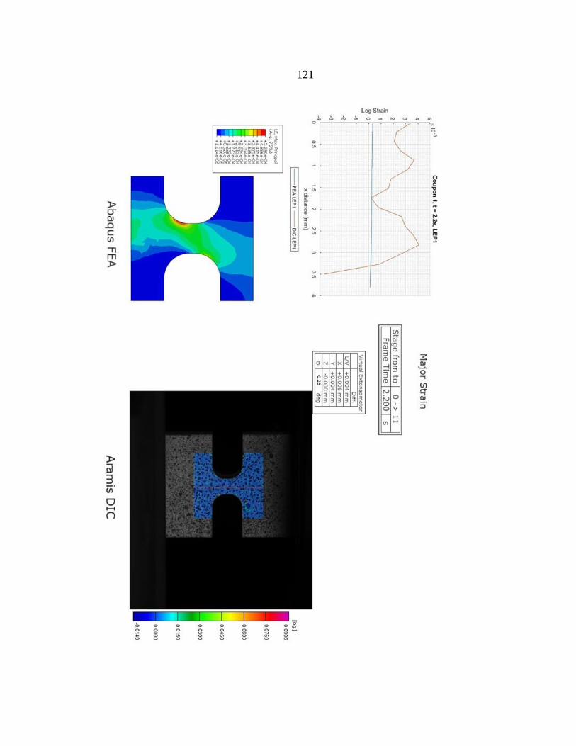
121

122

123

124

125

126

127

128

129

130

131

132

133

134

135

136

137

138

139

140

141

142

143

144

145

146

147

148
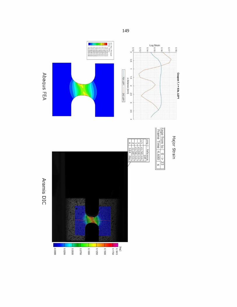
149

150

151

152

153

154

155

156

157

158

159

160

161

162

163

164

165

166