thomas glasdam jensen - technical university of...
TRANSCRIPT

Master Thesis, s011427
Acoustic radiation in microfluidicsystems
Thomas Glasdam Jensen
Supervisor: Henrik Bruus
MIC – Department of Micro and NanotechnologyTechnical University of Denmark
2 April 2007

ii

Abstract
As the Lab-On-a-Chip systems becomes increasingly sophisticated, so does the demandsto the embedded tools. This is why acoustic manipulation gain increasingly attentionaround the microfluidic community. Recent research have shown that carefully designedacoustic actuators can be used for both particle handling and mixing. Most research inthe micro-acousto-fluidic field is base on trial and error, as no well-developed theory existsin this area.
In this thesis we use perturbation theory to investigate the theory behind the acousticradiation force, and the equations describing the acoustic streaming flow-patterns. It showsthat the absolute amplitude of the acoustic radiation force is difficult to determine. How-ever, the calculated shape of the force corresponds very well to what have been reported byexperimentalists. The same thing is the case for the calculated streaming-patterns. Theshape of the patterns match the experimental ones very well, but the amplitude becomesseveral magnitudes larger than physical possible.
iii


Resume
Efterhanden som Lab-On-a-Chip systemerne bliver mere advancerede, øges kravene tilde indbyggede redskaber ogsa. Derfor er interessen for manipulation ved hjælp af akustikstigende i de mikrofluide kredse. Nylig forskning har vist, at man kan bruge nøje designedeakustiske resonnatorer til bade handtering af partikler samt til at mixe. Den primæreforskning pa det mikro-akustik-fluide omrade er baseret pa ’trial and error’-metoden, dader ikke eksisterer nogen fyldestgørende teori pa omradet.
I denne rapport gør vi brug af perturbations teori for at undersøge teorien bag denakustiske stralingskraft og ligningerne, der beskriver de akustiske strømningsmønstre. Detviser sig, at den absolutte størrelse pa stralingskraften er svær at finde, men den beregnedeform pa kraften ligner den, eksperimentalisterne har fundet. Det samme gør sig gældendefor de beregnede strømningsmønstre. Formen passer godt med den eksperimentielt fundne,men amplituderne bliver sa mange størelsesordner højere, at de ikke længere giver fysiskmening.
v


Preface
The thesis, hereby presented is titled ”Acoustic radiation in microfluidic systems”, it hasbeen submitted in order to obtain 50 ECTS points and the Master of Science degree atthe Technical University of Denmark (DTU).
This project was carried out within the Microfluidic Theory and Simulation (MIFTS)group at the Department of Micro- and Nanotechnology (MIC), DTU. The thesis waswritten during the period from April 2006 to April 2007 under supervision by HenrikBruus and in close collaboration with Ph.D. student Melker Sundin.
The purpose of this work have been to theoretically calculate the acoustic radiationforce and the acoustic streaming patterns observed during experiments performed in aearlier course. As this work is the first acoustic-related subject in the MIFTS-group, ithas been emphasized to derive the acoustic equations from the bottom, instead of acquiringthese from textbooks.
Finally I would like to thank my supervisor Henrik Bruus for his inspiring supportand for many fruitful discussions. And secondly, a thank to Melker Sundin for providingthe experimental basis, from which this project was inspired. I would also like to thankthe entire MIFTS-group for always being able to find a solution to (or way around) anyproblem encountered.
Thomas Glasdam JensenMIC – Department of Micro and Nanotechnology
Technical University of Denmark2 April 2007
vii


Contents
List of figures xiv
List of tables xv
List of symbols xvii
1 Introduction 11.1 The acoustic radiation force . . . . . . . . . . . . . . . . . . . . . . . . . . . 11.2 Acoustic streaming . . . . . . . . . . . . . . . . . . . . . . . . . . . . . . . . 21.3 Experimental background . . . . . . . . . . . . . . . . . . . . . . . . . . . . 3
1.3.1 The experimental setup . . . . . . . . . . . . . . . . . . . . . . . . . 31.3.2 The experimental results . . . . . . . . . . . . . . . . . . . . . . . . . 4
1.4 Material parameters . . . . . . . . . . . . . . . . . . . . . . . . . . . . . . . 5
2 Periodic motion in incompressible liquids 72.1 Dimensionless equations . . . . . . . . . . . . . . . . . . . . . . . . . . . . . 72.2 Perturbation in Pe for Re = 0 . . . . . . . . . . . . . . . . . . . . . . . . . . 8
2.2.1 Quasi-stationary Stokes flow; Pe = 0 . . . . . . . . . . . . . . . . . . 82.2.2 Stokes flow; Pe 6= 0 . . . . . . . . . . . . . . . . . . . . . . . . . . . . 102.2.3 Finding the full solution for Re = 0; Pe 6= 0 . . . . . . . . . . . . . . 12
2.3 Perturbation in Re . . . . . . . . . . . . . . . . . . . . . . . . . . . . . . . . 132.3.1 The quasi-stationary case, Pe = 0 . . . . . . . . . . . . . . . . . . . . 142.3.2 The Navier-Stokes case; Pe 6= 0 . . . . . . . . . . . . . . . . . . . . . 172.3.3 Solution for O(Pn
e ) and O(Re1) . . . . . . . . . . . . . . . . . . . . . 192.4 Comparing analytical and numerical solutions . . . . . . . . . . . . . . . . . 192.5 High-order terms . . . . . . . . . . . . . . . . . . . . . . . . . . . . . . . . . 21
2.5.1 Determination of u1n and p1n . . . . . . . . . . . . . . . . . . . . . . 212.5.2 Re to second order . . . . . . . . . . . . . . . . . . . . . . . . . . . . 232.5.3 Determination of vDC
3 . . . . . . . . . . . . . . . . . . . . . . . . . . 242.6 Concluding remarks . . . . . . . . . . . . . . . . . . . . . . . . . . . . . . . 25
3 Sound absorption in compressible liquids 273.1 Acoustic perturbation theory . . . . . . . . . . . . . . . . . . . . . . . . . . 273.2 The non-viscous case . . . . . . . . . . . . . . . . . . . . . . . . . . . . . . . 28
ix

x CONTENTS
3.2.1 Zeroth-order perturbation . . . . . . . . . . . . . . . . . . . . . . . . 283.2.2 First-order perturbation . . . . . . . . . . . . . . . . . . . . . . . . . 283.2.3 Second-order perturbation . . . . . . . . . . . . . . . . . . . . . . . . 30
3.3 The viscous case . . . . . . . . . . . . . . . . . . . . . . . . . . . . . . . . . 313.3.1 Zeroth-order perturbation . . . . . . . . . . . . . . . . . . . . . . . . 313.3.2 First-order perturbation . . . . . . . . . . . . . . . . . . . . . . . . . 313.3.3 Second-order perturbation . . . . . . . . . . . . . . . . . . . . . . . . 33
4 Planer sound waves 354.1 Wave-emission from an oscillating wall . . . . . . . . . . . . . . . . . . . . . 354.2 Wave propagation through a single interface . . . . . . . . . . . . . . . . . . 364.3 Wave propagation through multiple interfaces . . . . . . . . . . . . . . . . . 384.4 Acoustic Resonances . . . . . . . . . . . . . . . . . . . . . . . . . . . . . . . 41
4.4.1 Unattenuated waves . . . . . . . . . . . . . . . . . . . . . . . . . . . 414.4.2 Attenuated waves . . . . . . . . . . . . . . . . . . . . . . . . . . . . . 42
5 Numerical simulations in COMSOL 435.1 The Acoustic module in COMSOL . . . . . . . . . . . . . . . . . . . . . . . 43
5.1.1 The eigenfrequency solver . . . . . . . . . . . . . . . . . . . . . . . . 435.1.2 Example: Pseudo-one-dimensional . . . . . . . . . . . . . . . . . . . 445.1.3 The time harmonic solver . . . . . . . . . . . . . . . . . . . . . . . . 49
5.2 General PDE formulation for COMSOL . . . . . . . . . . . . . . . . . . . . 515.3 Executing a COMSOL-script . . . . . . . . . . . . . . . . . . . . . . . . . . 52
6 The acoustic radiation force 536.1 The force in one dimension . . . . . . . . . . . . . . . . . . . . . . . . . . . 536.2 The force in more dimensions . . . . . . . . . . . . . . . . . . . . . . . . . . 546.3 Dimensional analysis; from 3D to 2D . . . . . . . . . . . . . . . . . . . . . . 55
6.3.1 Validation of the 2D approximation . . . . . . . . . . . . . . . . . . 556.3.2 Density of states . . . . . . . . . . . . . . . . . . . . . . . . . . . . . 56
6.4 The symmetric chamber model . . . . . . . . . . . . . . . . . . . . . . . . . 586.5 Breaking of symmetry . . . . . . . . . . . . . . . . . . . . . . . . . . . . . . 606.6 Concluding remarks . . . . . . . . . . . . . . . . . . . . . . . . . . . . . . . 63
7 Examples of sound absorption in liquids 657.1 Analytic Example 1: plane traveling wave . . . . . . . . . . . . . . . . . . . 65
7.1.1 First order pressure, p1, and velocity u1 . . . . . . . . . . . . . . . . 657.1.2 Second order pressure, p′′2, and velocity u′′2 . . . . . . . . . . . . . . . 66
7.2 Analytic Example 2: Wave resonance, 1D . . . . . . . . . . . . . . . . . . . 697.2.1 First order pressure, p1, and velocity u1 . . . . . . . . . . . . . . . . 697.2.2 Second order pressure, p′′2, and velocity u′′2 . . . . . . . . . . . . . . . 70
7.3 Numeric Example 3: Wave resonance, 2D . . . . . . . . . . . . . . . . . . . 737.3.1 First order pressure, p1, and velocity u1 . . . . . . . . . . . . . . . . 737.3.2 Second order pressure, p′′2, and velocity u′′2 . . . . . . . . . . . . . . . 75

CONTENTS xi
8 Comparing theory and experiments 798.1 Simulated streaming patterns . . . . . . . . . . . . . . . . . . . . . . . . . . 798.2 Simulated radiation force . . . . . . . . . . . . . . . . . . . . . . . . . . . . 81
9 Conclusion 83
10 Outlook 85
Appendices 87
A COMSOL-script; Periodic motion in incompressible liquids 87
B COMSOL-script; Wave propagation through interfaces 91
C COMSOL-script; The symmetric chamber model 93
D COMSOL-script; Numeric Example 3 95


List of Figures
1.1 Chip-geometry used in experiments . . . . . . . . . . . . . . . . . . . . . . . 31.2 Chip photo . . . . . . . . . . . . . . . . . . . . . . . . . . . . . . . . . . . . 41.3 Experimental results for large particles . . . . . . . . . . . . . . . . . . . . . 41.4 Experimental results for small particles . . . . . . . . . . . . . . . . . . . . 5
2.1 Contour plot of ψqua . . . . . . . . . . . . . . . . . . . . . . . . . . . . . . . 92.2 Contour plot of ψsto . . . . . . . . . . . . . . . . . . . . . . . . . . . . . . . 132.3 Contour plot of ψPe=0 . . . . . . . . . . . . . . . . . . . . . . . . . . . . . . 172.4 Contour plot of ψ . . . . . . . . . . . . . . . . . . . . . . . . . . . . . . . . . 182.5 Plot of AAV, Re = 10 Pe . . . . . . . . . . . . . . . . . . . . . . . . . . . . 202.6 Error plot, Re = 10 Pe . . . . . . . . . . . . . . . . . . . . . . . . . . . . . . 202.7 Plot of AAV, Re = 2 Pe . . . . . . . . . . . . . . . . . . . . . . . . . . . . . 212.8 Error plot, Re = 2 Pe . . . . . . . . . . . . . . . . . . . . . . . . . . . . . . 21
4.1 A planar wave . . . . . . . . . . . . . . . . . . . . . . . . . . . . . . . . . . . 364.2 A wave passing multiple interfaces . . . . . . . . . . . . . . . . . . . . . . . 384.3 Particle velocity and pressure, on and off-resonance . . . . . . . . . . . . . . 40
5.1 Pseudo-1D geometry . . . . . . . . . . . . . . . . . . . . . . . . . . . . . . . 455.2 Mesh for Pseudo-1D geometry . . . . . . . . . . . . . . . . . . . . . . . . . . 455.3 Plot of pressure at eigenfrequency . . . . . . . . . . . . . . . . . . . . . . . 485.4 Numeric validation (resonance) . . . . . . . . . . . . . . . . . . . . . . . . . 505.5 Errorplot(resonance) . . . . . . . . . . . . . . . . . . . . . . . . . . . . . . . 505.6 Numeric validation (non-resonance) . . . . . . . . . . . . . . . . . . . . . . . 515.7 Errorplot(non-resonance) . . . . . . . . . . . . . . . . . . . . . . . . . . . . 51
6.1 Cell seperation . . . . . . . . . . . . . . . . . . . . . . . . . . . . . . . . . . 546.2 3D sorted eigenfrequencies . . . . . . . . . . . . . . . . . . . . . . . . . . . . 566.3 3D sorted eigenfrequencies . . . . . . . . . . . . . . . . . . . . . . . . . . . . 566.4 Density of states . . . . . . . . . . . . . . . . . . . . . . . . . . . . . . . . . 576.5 Analytical density of states . . . . . . . . . . . . . . . . . . . . . . . . . . . 586.6 The chamber model geometry . . . . . . . . . . . . . . . . . . . . . . . . . . 596.7 Exampels of eigenmodes . . . . . . . . . . . . . . . . . . . . . . . . . . . . . 606.8 Sketch of asymmetric models . . . . . . . . . . . . . . . . . . . . . . . . . . 61
xiii

xiv LIST OF FIGURES
6.9 Comparison of asymmetric patterns . . . . . . . . . . . . . . . . . . . . . . 62
7.1 Acoustic radiation force - 1D . . . . . . . . . . . . . . . . . . . . . . . . . . 717.2 First order pressure, p1 - 2D . . . . . . . . . . . . . . . . . . . . . . . . . . . 747.3 Time averaged first order flux . . . . . . . . . . . . . . . . . . . . . . . . . . 757.4 Divergence of second order velocity, S - 2D . . . . . . . . . . . . . . . . . . 767.5 Force density, F ′′
x and F ′′y - 2D . . . . . . . . . . . . . . . . . . . . . . . . . 77
7.6 Numeric results - 2D . . . . . . . . . . . . . . . . . . . . . . . . . . . . . . . 78
8.1 Vortices - 6× 6 and 2× 2 . . . . . . . . . . . . . . . . . . . . . . . . . . . . 808.2 Acoustic radiation force; vector-plot . . . . . . . . . . . . . . . . . . . . . . 818.3 Acoustic radiation force; cross-section . . . . . . . . . . . . . . . . . . . . . 82

List of Tables
1.1 Material parameters . . . . . . . . . . . . . . . . . . . . . . . . . . . . . . . 6
2.1 Numerical simulation parameters . . . . . . . . . . . . . . . . . . . . . . . . 19
5.1 Domain groups . . . . . . . . . . . . . . . . . . . . . . . . . . . . . . . . . . 465.2 Boundary groups . . . . . . . . . . . . . . . . . . . . . . . . . . . . . . . . . 47
xv

xvi LIST OF TABLES
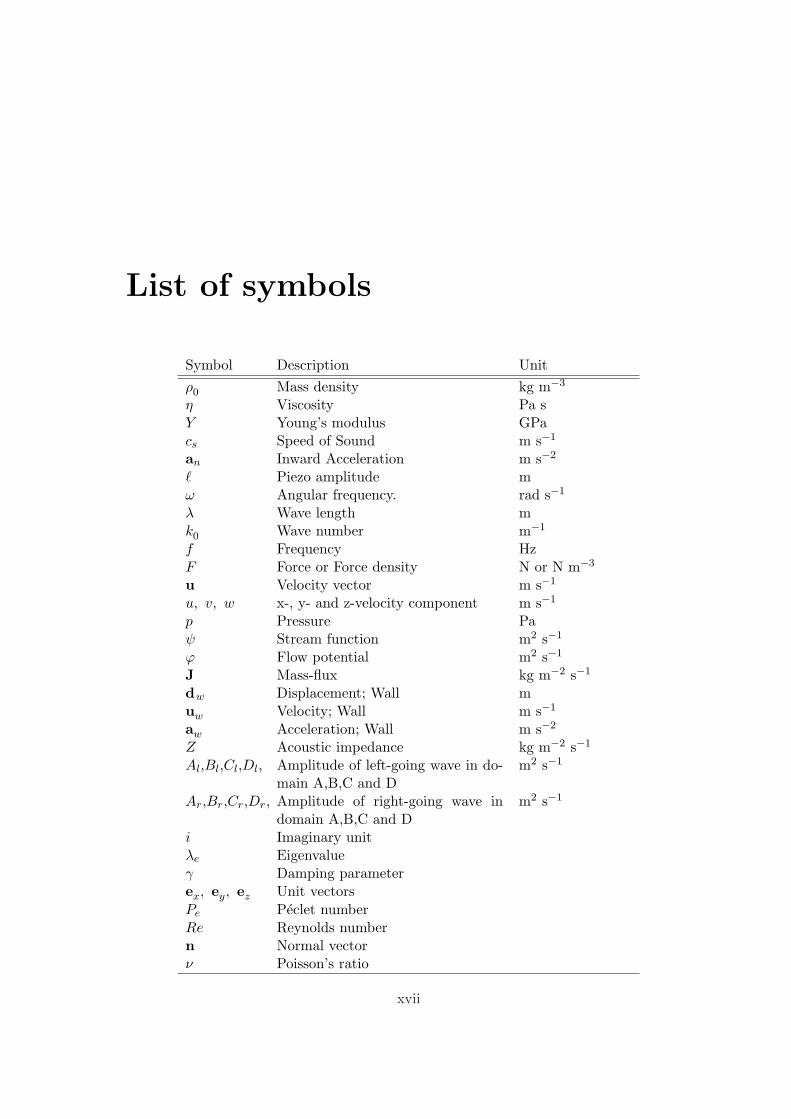
List of symbols
Symbol Description Unitρ0 Mass density kg m−3
η Viscosity Pa sY Young’s modulus GPacs Speed of Sound m s−1
an Inward Acceleration m s−2
` Piezo amplitude mω Angular frequency. rad s−1
λ Wave length mk0 Wave number m−1
f Frequency HzF Force or Force density N or N m−3
u Velocity vector m s−1
u, v, w x-, y- and z-velocity component m s−1
p Pressure Paψ Stream function m2 s−1
ϕ Flow potential m2 s−1
J Mass-flux kg m−2 s−1
dw Displacement; Wall muw Velocity; Wall m s−1
aw Acceleration; Wall m s−2
Z Acoustic impedance kg m−2 s−1
Al,Bl,Cl,Dl, Amplitude of left-going wave in do-main A,B,C and D
m2 s−1
Ar,Br,Cr,Dr, Amplitude of right-going wave indomain A,B,C and D
m2 s−1
i Imaginary unitλe Eigenvalueγ Damping parameterex, ey, ez Unit vectorsPe Peclet numberRe Reynolds numbern Normal vectorν Poisson’s ratio
xvii

Chapter 1
Introduction
One of the rare instances where the non-linear inertia term ρ(u·∇)u plays a significant rolein microfluidics relates to acoustic radiation in liquids. The non-linearity of the term makesthe existence of a non-zero time-averaged velocity component possible for a system whereharmonically oscillating acoustic waves has been emitted into the liquid. Thus acousticradiation may be the source of a direct-current liquid flow field[1]. The non-linear termmight also result in non-zero time-averaged pressure field, which can be used for particlemanipulation. This thesis will study both the flow-patterns induced by an acoustic field,and on the acoustic radiation force affecting any suspended particles.
1.1 The acoustic radiation force
In many µTAS applications there is a need for sorting or separating the input parti-cles. This could for instance be an input consisting of different biological molecules orcells. If the concerning analysis is only to be conducted on one type of particles, thenit is sometimes necessary to remove the other particles from the sample. There are sev-eral very different methods of separating particles. One of the most obvious methods isthe bumper-array[2], which sorts the particles by size. By making a fine grid inside thechannels, the larger particles is forced towards a different outlet than the smaller ones.Another way of separating particles is by exploiting that particles with different electricalcharge will move with different speed when placed in an electric field. This technique isknown as electrophoresis[3, 4, 5]. A third method is dielectrophoresis, which will workon charge neutral particles. Dielectrophoresis works if there is a difference between thedielectric constant of the of a particle and the liquid surrounding it[6, 7]. A fourth separa-tion technique is magnetophoresis, where magnetic micro beads, coated with appropriateantibodies, bind to the targeted particles[8, 9].
The fifth method is by use of the acoustic radiation force. If the density and com-pressibility of the suspended particles and the surrounding fluid has a given ratio, then itis possible to control the particles. In 1935 L. V. King [10] calculated the acoustic effectson hard circular discs. The theory was further developed by Yosioka and Kawasima[11]in 1955. The theory is however only derived for a planar wave system, and have not beenconsiderably improved since. Hence, to this day scientists[12, 13, 14, 15, 16, 17] must
1

Chapter 1 Introduction
suffice with the planar wave theory, when explaining their results. During this thesis weshall develop a method for calculating the shape(only relative amplitudes) of the acousticradiation force in three dimensions. The use of acoustic forces in microfluidic systems is arelatively new idea, and only a few applications have been presented.
The article by H. Li and T. Kenny[17] points out that one of the greater challengeswhen developing a handheld portable blood diagnosis device, is the separation of theblood constituents. They propose a device based on separation using acoustic radiationas a possible solution.
Another application is presented by Jonsson, H et al.[18]. They argue that the embolicload experienced by patients undergoing cardiac surgery, can be greatly reduced by usingacoustic radiation to remove lipid particles from the recirculating blood.
One of the expected strengths of these acoustic applications is the ability to handleliving cells without harming them.
1.2 Acoustic streaming
In microfluidic systems the flow velocity is often very low and as result thereof the flowbecomes laminar. As the word ’laminar’ implies, the fluid consists of layers, which almostdoes not mix. Due to the laminar nature(compared to turbulent) mixing is only caused bydiffusion[19]. Even though the length scales in microsystem are very small the diffusion isoften too slow to provide sufficient mixing. The easiest way to achieve a good mixing isto make the fluidic channel so long that diffusion has time enough to perform the mixing.The long channels are often constructed in meander-shapes. Of other methods for mixinglaminar fluids we can mention oscillatory pumping of either the main inlet/outlet or asecondary pair of inlets [20]. Another method is designing a chamber were the inletscreates an unbalanced driving force, making the liquid swirl around[21, 22]. A slightlymore complex method is that of electro-osmotic induced mixing[23], where the oscillatingcharge on the chamber walls create a non-zero slip velocity. A fifth possibility is to useacoustic streaming. Acoustic streaming is the name of the flow induced in a fluid by anacoustic source.
Acoustic streaming was first described by Lord Rayleigh in the late 1880’ies. It wasfurther developed by C. Eckart[24] in 1947, J. Markham[25] in 1951 and by W. Nyborg[26]in 1952. The results from these three articles have been used as inspiration for developingthe equations in Chapter 3. The use of acoustic streaming have been very limited, it hasmainly been used for teaching purposes in form of the kundt’s tube. Only recently, as thelab-on-chip systems becomes more sophisticated the need of effective mixing has increasedand the first applications are being developed.
In December 2005 the EU-funded project SMART-BioMEMS started[27]. The projectevolves around testing for generic mutation. During the sample handling, mixing is re-quired. According to plan, the mixing should be achieved by acoustic streaming, inducedby a piezo-element.
2

Experimental background Section 1.3
1.3 Experimental background
In the early spring 2006, I participated in an experimental special-course with the purposeof investigating the acoustic radiation force and acoustic streaming experimentally. Thecoursed was supervised by Jorg Kutter and Melker Sundin at MIC, DTU. Due to the poorunderstanding of the experimentally achieved results, I started the work on this Masterthesis. Hence, the workload for this thesis has been solely theoretical, all references toexperimental work, is refereing to work earlier performed and already credited, or toexperimental work performed by Melker Sundin.
1.3.1 The experimental setup
The chip, which was use in the experiments, consists of three layers. The chip is sketchedin Fig. 1.1. The lower layer consists of silicon with etched holes for in- and outlet. Themiddle layer also consists of silicon, in this layer channels have been etched. During theexperiments, these channels were filled with water, in which particles were suspended. Theupper layer is a pyrex plate. This is used to seal of the channels, while providing opticalaccess. In reality the two lower layers in Fig. 1.1 are actually only one layer. However, toclarify the description these are shown separated. The silicon wafer were 500 µm thick,and the channel were etched to have a depth of 200 µm. Hence, the bottom layer has athickness of 300 µm, and the middle layer is 200 µm. The top layer has the thickness ofa pyrex wafer, 500 µm. The width of the chip is 15 mm and the length is 47.2 mm. Theentire length of the channel is 25 mm and the chamber measures 2× 2 mm. Notice thatthe chip depiction in Fig. 1.1 only sketches the geometry, objects are plotted with differentlength scales. A photo of the real chip is shown in Fig. 1.2
Water
300 µm
200 µm
500 µm
15 mm
47.2 mm
Pyrex
Silicon
Silicon
x
y
z
Figure 1.1: The chip layout, divided into three layers.
Experiments were also conducted on a similar chip, but with a round chamber witha diameter of 2 mm. Two different types of particles were used in the experiments. Thefirst kind was polystyrene beads with a diameter of 10 µm, these beads were chosen sincethey have similar physical properties as red blood cells. The second type of particleswere diluted milk containing lipid-particles of approximately 1 µm diameter. When theexperiments were conducted, the microscope was located above the chip, looking down
3
Chapter 1 Introduction
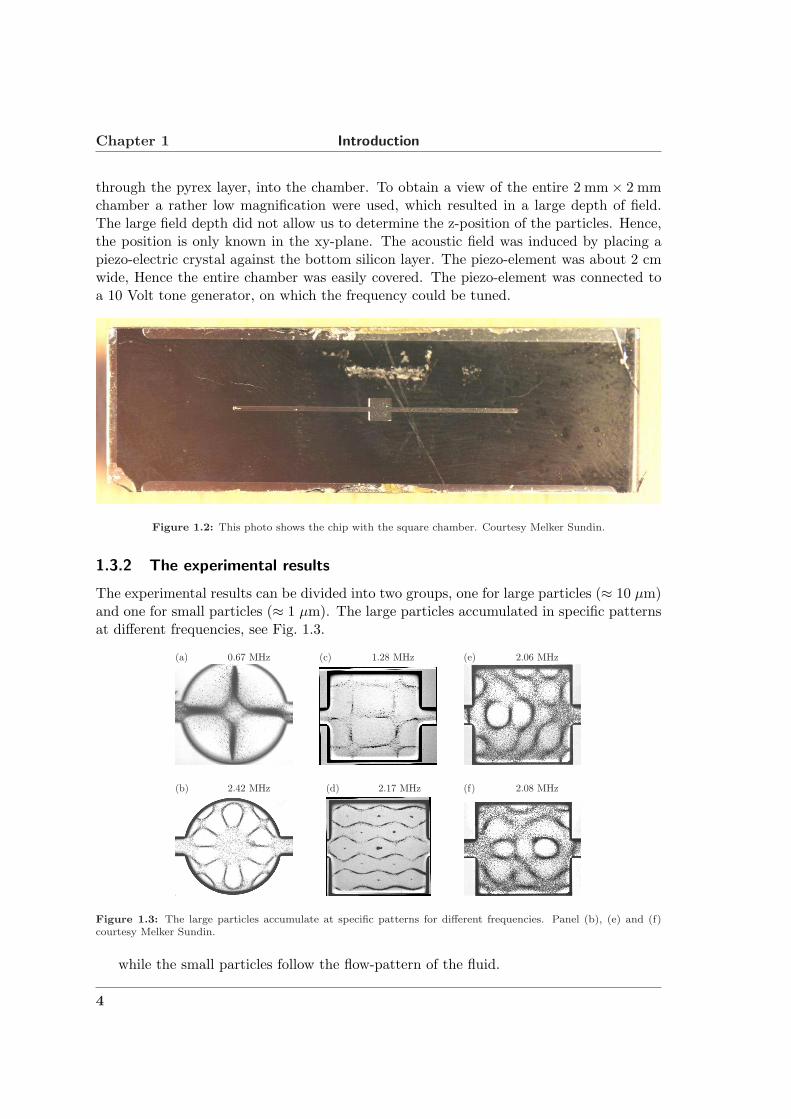
through the pyrex layer, into the chamber. To obtain a view of the entire 2 mm× 2 mmchamber a rather low magnification were used, which resulted in a large depth of field.The large field depth did not allow us to determine the z-position of the particles. Hence,the position is only known in the xy-plane. The acoustic field was induced by placing apiezo-electric crystal against the bottom silicon layer. The piezo-element was about 2 cmwide, Hence the entire chamber was easily covered. The piezo-element was connected toa 10 Volt tone generator, on which the frequency could be tuned.
Figure 1.2: This photo shows the chip with the square chamber. Courtesy Melker Sundin.
1.3.2 The experimental results
The experimental results can be divided into two groups, one for large particles (≈ 10 µm)and one for small particles (≈ 1 µm). The large particles accumulated in specific patternsat different frequencies, see Fig. 1.3.
(a) 0.67 MHz
(b) 2.42 MHz
(c) 1.28 MHz
(d) 2.17 MHz
(e) 2.06 MHz
(f) 2.08 MHz
Figure 1.3: The large particles accumulate at specific patterns for different frequencies. Panel (b), (e) and (f)courtesy Melker Sundin.
while the small particles follow the flow-pattern of the fluid.
4

Material parameters Section 1.4
Figure 1.4: A PIV-image, showing the steady state velocity(≈ 0.5 mm/s) of the particles at 2.17 MHz. CourtesyMelker Sundin
We notice that that for the a frequency of 2.17 MHz, we see two different results forparticles of different size.
The rest of this thesis will be an attempt to theoretically explain how and why thesepatterns exists.
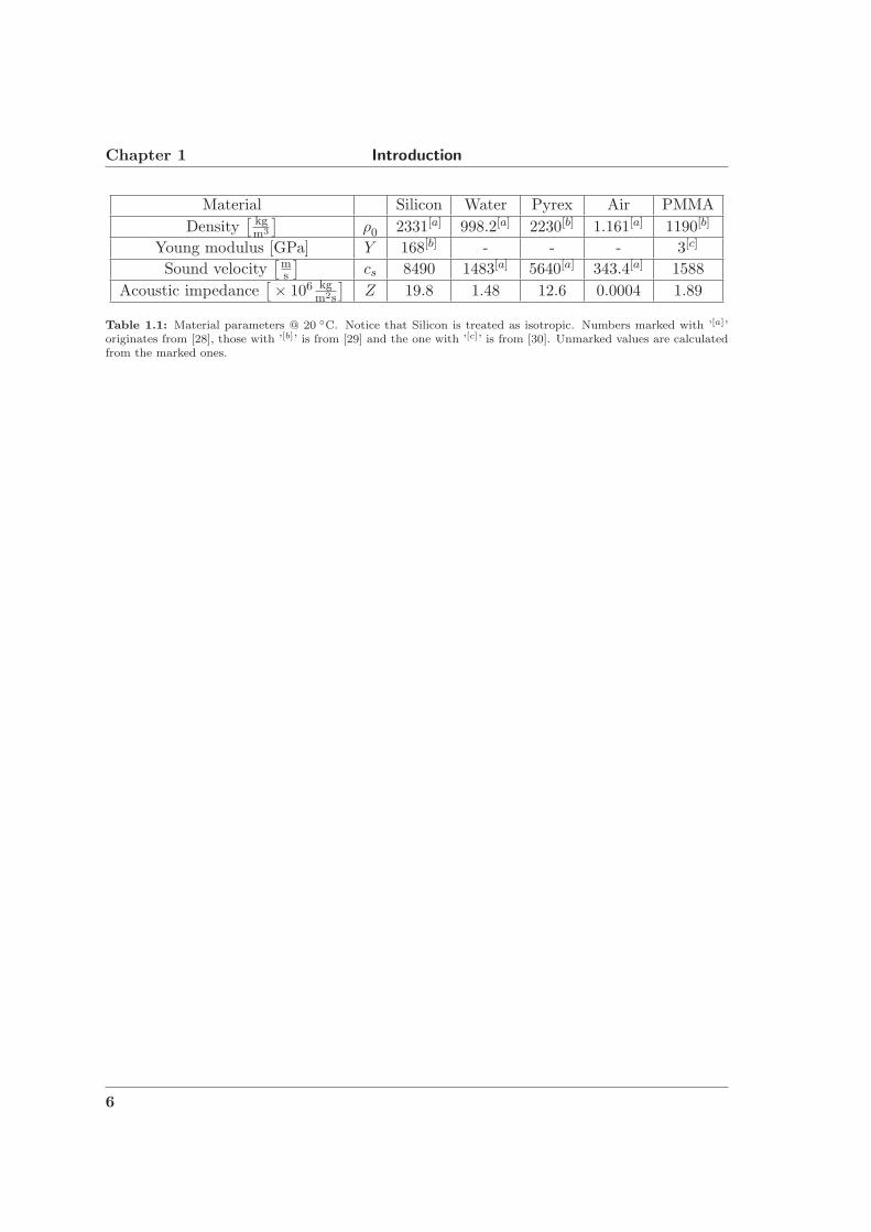
1.4 Material parameters
Before we calculate any thing, we are going to need some material parameters. In acousticsthe important parameters are the density, ρ0, and the speed of sound, cs. In solids thespeed of sound has two different definitions. One for objects with dimensions close to thewavelength, and another for larger objects. For small objects cs is defined as
cs =
√Y
ρ0
, (1.1)
where Y is Young’s modulus. This is the equation we will use when performing calculationson microsystems. The sound velocity for Silicon and PMMA in Table 1.1 is calculated usingthis. For structures much larger than the wavelength the definition must also include thePoisson’s ratio ν. We notice that that for Silicon the Young’s modulus is lattice dependant.We shall however assume that Silicon is an isotropic material and hence, use the averagemodulus instead.
5
Chapter 1 Introduction
Material Silicon Water Pyrex Air PMMADensity
[ kgm3
]ρ0 2331[a] 998.2[a] 2230[b] 1.161[a] 1190[b]
Young modulus [GPa] Y 168[b] - - - 3[c]
Sound velocity[
ms
]cs 8490 1483[a] 5640[a] 343.4[a] 1588
Acoustic impedance[× 106 kg
m2s
]Z 19.8 1.48 12.6 0.0004 1.89
Table 1.1: Material parameters @ 20 C. Notice that Silicon is treated as isotropic. Numbers marked with ’[a]’originates from [28], those with ’[b]’ is from [29] and the one with ’[c]’ is from [30]. Unmarked values are calculatedfrom the marked ones.
6

Chapter 2
Periodic motion in incompressible liquids
When describing microfluidic systems containing a water-like liquid, we usually assumethat the liquid is incompressible. However, if the liquid is incompressible, sound wavescan not be propagated. Our attempt to calculate the acoustic radiation force and acousticstreaming, are therefore limited by our choice of compressibility. In this chapter we inves-tigate the basic properties of an oscillating boundary and its effects on an incompressibleliquid. Perhaps the motion of the boundary is enough to account for the experimentallyobserved phenomenons. In Chapter 3 we look at compressible liquids.
2.1 Dimensionless equations
We consider the half-space z > 0 bounded by the xy plane at z = 0 and otherwiseunbounded. The oscillating motion is assumed generated by applying an AC-voltage ofangular frequency ω to an infinite array of equidistant interdigitated, flat electrodes spacedby λ = 2π/k on top of a piezo-electric crystal. This setup is modeled by the standing-waveslip-boundary condition at z = 0 and no-slip at z = ∞,
u(x, y, z, t) = (u ex, v ey, w ez) (2.1a)
u(x, y, 0, t) = u0 cos(kx) eiωt ex, (2.1b)u(x, y,∞, t) = 0, (2.1c)
where we have used complex notation for the time dependence. Given these boundaryconditions, the goal of this chapter is to solve the Navier–Stokes equation (Eq. (2.2)) foran incompressible liquid
ρ[∂tu + (u·∇)u
]= η∇2u−∇p, (2.2)
where p = p(x, y, z, t) is the pressure field.The system can be characterized by two dimensionless parameters, the Peclet number
Pe and the Reynolds number Re, given by
Pe ≡ ρω
k2η, (2.3a)
7

Chapter 2 Periodic motion in incompressible liquids
Re ≡ ρu0
kη. (2.3b)
If we furthermore introduce the following dimensionless variables denoted by a underline,
r =1kr, u = u0u, p = (kηu0)p, t =
1ω
t, (2.4)
the problem, including the incompressible continuity equation, takes the following dimen-sionless form,
Pe∂tu + Re (u·∇)u = ∇2u−∇p, (2.5a)∇·u = 0, (2.5b)
u(x, y, 0, t) = cos(x) eit ex, (2.5c)u(x, y,∞, t) = 0. (2.5d)
Here we have already dropped the underline as we only will use dimensionless variables inthe rest of this chapter.
Finally, if we utilize that the translation invariance along the y-axis results in thesimple 2D velocity field u(r, t) =
(u(x, z, t), w(x, z, t)
)we arrive at the final formulation
of our problem:
[Pe∂t + Re (u∂x + w∂z)
]( uw
)=
(∂2
x + ∂2z
)( uw
)−
(∂xp∂zp
), (2.6a)
∂xu + ∂zw = 0, (2.6b)(
u(x, 0, t)w(x, 0, t)
)=
(cos(x) eit
0
), (2.6c)
(u(x,∞, t)w(x,∞, t)
)=
(00
). (2.6d)
2.2 Perturbation in Pe for Re = 0
2.2.1 Quasi-stationary Stokes flow; Pe = 0
The limit of quasi-stationary Stokes flow is particularly simple to solve, as both Pe andRe are zero, and Eq. (2.6a) becomes
(∂2
x + ∂2z
)( uw
)=
(∂xp∂zp
). (2.7)
By employing the so-called stream function ψ(x, z, t), related to the velocity field by theexpression (
uw
)≡
(+∂zψ−∂xψ
), (2.8)
8

Perturbation in Pe for Re = 0 Section 2.2
the incompressibility condition ∂xu + ∂zw = 0 is automatically fulfilled. We also noteby taking the divergence of the Stokes equation and utilizing ∇ ·u = 0 we find that thepressure fulfills the Laplace equation
(∂2
x + ∂2z
)p = 0. (2.9)
To find the solution u to our problem, we begin by noting that u(x, 0) = cos(x). Thisperiodic behavior must also be reflected in the pressure, but as p must fulfill the Laplaceequation, we are led to guess the following solution p ∝ f(x) e−z. This exponential fall-off, on the other hand, must be reflected back to the behavior of the velocity field awayfrom z = 0. Thus, it is reasonable to guess that the stream function must be of the formψqua ∝ cos(x)e−z, but to ensure a vanishing z-component of the velocity, we throw in anextra factor z and arrive at
ψqua = cos(x) z e−z. (2.10)
Using the definition from Eq. (2.8) we get:
u = uqua =(
uw
)=
(cos(x) [1− z] e−z
sin(x) z e−z
), (2.11)
and also
∇2uqua =(
2 cos(x) e−z
−2 sin(x) e−z
)= ∇p. (2.12)
From this it can be seen that
p = pqua = 2 sin(x) e−z. (2.13)
x
z
0 1 2 3 4 5 60
1
2
3
4
5
6
Figure 2.1: Contour plot of ψqua. It can be seen that a row of rolls are located along the actuating boundary(x=0).We notice that the rolls only stretch ≈ λ into the liquid. We can see from the gradient of ψqua that the velocity ishighest at the wall.
9

Chapter 2 Periodic motion in incompressible liquids
2.2.2 Stokes flow; Pe 6= 0
To solve the problem with Re = 0 and Pe 6= 0 we use a perturbation method. Because ofthe oscillating boundary condition both pressure and velocity is expected to be oscillating.Hence, each term in p and u must be of the form:
p(x, z, t) = p(x, z)eit = p eit, (2.14a)
u(x, z, t) = u(x, z)eit = u eit, (2.14b)
by differentiating u with time, removing all eit-factors by division Eq. (2.6a) becomes[(
∂2x + ∂2
z
)− i Pe
]u = ∇p, (2.15)
u and p are spilt up in terms of different order of Pe:
u = u0 + Peu1 + P 2e u2 + P 3
e u3 + . . . , (2.16a)
p = p0 + Pep1 + P 2e p2 + P 3
e p3 + . . . , (2.16b)
and hence, the governing equation becomes
[(∂2
x + ∂2z
)− i Pe
](u0 + Peu1 + P 2
e u2 + P 3e u3 + . . .
)= ∇
(p0 + Pep1 + P 2
e p2 + P 3e p3 + . . .
).
(2.17)
To solve this the equation, it is split into terms of different order of Pe:
O(P 0e ) : ∇2u0 = ∇p0, (2.18a)
O(P 1e ) : ∇2u1 − i u0 = ∇ p1, (2.18b)
O(P 2e ) : ∇2u2 − i u1 = ∇p2, (2.18c)
O(P 3e ) : . . . . (2.18d)
These equations can be solved by inserting the results from the first in the second, and soon. The first equation has already been solved in Section 2.2.1. We see that
u0 = u0,sto = uqua. (2.19)
p0 = p0,sto = pqua. (2.20)
To find u1 in the O(P 1e ) equation, we must first guess a streamfunction. To aid our
guess we look at the boundary condition u(x, 0) = cos(x). Since u0(x, 0) = cos(x) thenun(x, 0) = 0. Notice the difference between the zeroth-order velocity in the x-direction,u0(x, t), and the velocity amplitude of the boundary, u0. This lead to the streamfunctionguess:
ψn = cos(x) zn+1 e−z. (2.21)
By modifying the definition of the streamfunction to:(
un
wn
)≡ cn
(+∂zψn
−∂xψn
)≡ cnvn, (2.22)
10

Perturbation in Pe for Re = 0 Section 2.2
we get:
u1 = c1
(cos(x) e−z [2z − z2]
sin(x) e−z z2
)= c1v1. (2.23)
Since ∇2u1 = c1 ∇2v1, Eq. (2.18b) becomes
c1∇2v1 − i u0 = ∇ p1, (2.24)
where
∇2v1 =(
cos(x) e−z [4z − 6]sin(x) e−z [2− 4z]
)= −∇p0 − 4u0. (2.25)
Hencec1
(∇p0 − 4u0
)− i u0 = ∇ p1. (2.26)
This equation can be fulfilled by setting c1 = −i4 and p1 = c1 p0. This results in
u1 = u1,sto =−i
4
(cos(x) e−z [2z − z2]
sin(x) e−z z2
), (2.27a)
p1 = p1,sto =(−i
4
)2 sin(x) e−z. (2.27b)
Next we solve the O(P 2e ) equation: ∇2u2 − i u1 = ∇p2. By combining Eq. (2.21) and
Eq. (2.22) we get
u2 = c2
(cos(x) e−z [3z2 − z3]
sin(x) e−z z3
)= c2v2. (2.28)
Since ∇2u2 = c2 ∇2v2, Eq. (2.18c) becomes
c2∇2v2 − i u1 = ∇ p2. (2.29)
We start by looking at ∇2v2:
∇2v2 =(
cos(x) e−z [6− 18z + 6z2]sin(x) e−z [6z − 6z2]
)= 6u0 − 6v1 = 6u0 − i 24 u1, (2.30)
so that−i 16 u1 =
23∇2v2 − 4 u0. (2.31)
Substituting 4 u0 using the relation in Eq. (2.25) we get−i
4∇ p1 = ∇2
[− 1
24v2 −
i
4u1
]− i u1. (2.32a)
Hence if
u2 = u2,sto = − 124
v2 −i
4u1, (2.33a)
p2 = p2,sto =−i
4p1 =
116
p0, (2.33b)
the equation is fulfilled. So for Re = 0 we get the approximate solution
usto ≈ u0,sto + Peu1,sto + P 2e u2,sto +O(P 3
e )
≈ e−z
(cos(x)
[(1− z)− iPe
4 (2z − z2)− P 2e
48 (6z + 3z2 − 2z3)]
sin(x)[z − iPe
4 z2 − P 2e
48 (3z2 + 2z3)]
)+O(P 3
e ).(2.34)
11

Chapter 2 Periodic motion in incompressible liquids
2.2.3 Finding the full solution for Re = 0; Pe 6= 0
The differential equation in Eq. (2.15) can also be solved by guessing the right solution.From the results in Section 2.2.2, we guess that p = A p0 = 2 A sin(x) e−z and thatψ(x, z) = cos(x) h(z) e−z. Where h(z) is a function to be guessed. By differentiating thestreamfunction, ψ we get the velocity
u =(
∂zψ−∂xψ
)=
(cos(x) e−z [h′(z)− h(z)]
sin(x) e−z h(z)
). (2.35)
Inserting u and p into Eq. (2.15) yields:
[∇2 − iPe
]( cos(x) e−z [h′ − h]sin(x) e−z h
)= ∇[
2 A sin(x) e−z],
(cos(x) e−z [2h′ − 3h′′ + h′′′]
sin(x) e−z [h′′ − 2h′]
)− iPe
(cos(x) e−z [h′ − h]
sin(x) e−z h
)=
(2A cos(x) e−z
−2A sin(x) e−z
).
(2.36)
This leaves us with the following two equations:
2h′ − 3h′′ + h′′′ − i Pe h′ + i Pe h = 2 A, (2.37a)h′′ − 2 h′ − i Pe h = −2 A. (2.37b)
Adding the two equations together gives a third:
−2h′′ + h′′′ − i Pe h′ = 0. (2.38)
From Eq. (2.38) we can see that one solution could be h(z) = B, where B is a constant.However, to fulfill the boundary conditions for h(z), which are found from Eq. (2.6c),Eq. (2.6d) and Eq. (2.35) to be
h(0) = 0, (2.39a)h′(0) = 1, (2.39b)h(∞) = 0, (2.39c)
we guess:h(z) = B(1− eα z). (2.40)
Inserting h(z) into Eq. (2.38) gives
−[−2 α2 + α3 − i Pe α] B eα z = 0. (2.41)
B eα z is divided out and the resulting quadratic equation in α has the two solutions
α∓ = 1∓√
1 + i Pe. (2.42)
using h(∞) = 0 we get α = α−, and from h′(0) = 1 we get
B =−1α
=1√
1 + i Pe − 1. (2.43)
12

Perturbation in Re Section 2.3
All that remain is to determine A. This is done by inserting h(z) into Eq. (2.37b) andsolving for A
A =−i Pe
2α=
i Pe
2(√
1 + i Pe − 1). (2.44)
To summarize we got:
ψsto = cos(x) e−z 1√1 + iPe − 1
(1− ez−z√
1+iPe), (2.45a)
usto =
(cos(x)
√1+iPe e−z
√1+iPe−e−z√
1+iPe−1
sin(x) e−z√
1+iPe−e−z
1−√1+iPe
), (2.45b)
psto =i Pe sin(x) e−z
√1 + i Pe − 1
. (2.45c)
x
z
0 1 2 3 4 5 60
1
2
3
4
5
6
Figure 2.2: Contour plot of ψsto, where Pe = 1. It can be seen that the row of rolls does not stretch as far intothe liquid as in the quasi-stationary case.
2.3 Perturbation in Re
To solve Eq. (2.5a) for Pe 6= 0 and Re 6= 0 we once more use a perturbation method. Webegin by rewriting Eq. (2.5a) to
[∇2 − Pe ∂t − Re(u·∇)
]u = ∇p, (2.46)
where
u = u0 + Re u1 + Re2 u2 + Re3 u3 + . . . , (2.47a)
13

Chapter 2 Periodic motion in incompressible liquids
p = p0 + Re p1 + Re2 p2 + Re3 p3 + . . . . (2.47b)
Splitting Eq. (2.46) into terms of different order of Re yields
O(Re0) :[∇2 − Pe∂t
]u0 −∇p0 = 0 (2.48a)
O(Re1) :[∇2 − Pe∂t
]u1 −∇p1 = (u0 ·∇)u0, (2.48b)
O(Re2) :[∇2 − Pe∂t
]u2 −∇p2 = (u1 ·∇)u0 + (u0 ·∇)u1, (2.48c)
O(Re3) : . . . . (2.48d)
It is recognized that for Pe 6= 0 Eq. (2.48a) is the same as Eq. (2.15). Hence we got
u0 = usto =
(cos(x)
√1+iPe e−z
√1+iPe−e−z√
1+iPe−1
sin(x) e−z√
1+iPe−e−z
1−√1+iPe
), (2.49a)
p0 = psto =i Pe sin(x) e−z
√1 + i Pe − 1
, (2.49b)
and for Pe = 0 Eq. (2.48a) is the same as Eq. (2.7), hence,
u0 = uqua =(
cos(x) [1− z] e−z
sin(x) z e−z
), (2.50a)
p0 = pqua = 2 sin(x) e−z. (2.50b)
2.3.1 The quasi-stationary case, Pe = 0
First we solve the equation in O(Re1), for Pe = 0. Eq. (2.48b) becomes
∇2u1 −∇p1 = (u0 ·∇)u0, where u0 = uqua. (2.51)
Since we assume the system is to be used at high frequencies(≈ 1 MHz), we are notinterested in the velocities at small time scales and hence, we look at the time-averagedproblem, where
〈. . .〉t =1T
T∫
0
. . .dt. (2.52)
〈∇2u1〉t − 〈∇p1〉t = 〈(uqua ·∇)uqua〉t. (2.53)
To get rid of artificial real terms, originating from imaginary cross-products, we only usethe real part of uqua, since it appears in a nonlinear term
uqua ≡ Re[uquaeit] ≡ Re[uqua] cos(t)− Im[uqua] sin(t). (2.54)
Hence, we got
(uqua ·∇)uqua =([
Re[uqua] cos(t)− Im[uqua] sin(t)]·∇
)
×[Re[uqua] cos(t)− Im[uqua] sin(t)
]
14

Perturbation in Re Section 2.3
= + (Re[uqua] cos(t)·∇)Re[uqua] cos(t)
− (Re[uqua] cos(t)·∇)Im[uqua] sin(t)
− (Im[uqua] sin(t)·∇)Re[uqua] cos(t)
+ (Im[uqua] sin(t)·∇)Im[uqua] sin(t)
= + cos2(t)(Re[uqua]·∇)Re[uqua]
− cos(t) sin(t)(Re[uqua]·∇)Im[uqua]
− sin(t) cos(t)(Im[uqua]·∇)Re[uqua]
+ sin2(t)(Im[uqua]·∇)Im[uqua]
= +cos(2t)
2(Re[uqua]·∇)Re[uqua]
− sin(2t)2
(Re[uqua]·∇)Im[uqua]
− sin(2t)2
(Im[uqua]·∇)Re[uqua]
− cos(2t)2
(Im[uqua]·∇)Im[uqua]
+12(Re[uqua]·∇)Re[uqua]
+12(Im[uqua]·∇)Im[uqua]
(2.55)
when time averaging this we find that
〈(uqua ·∇)uqua〉t =12
[Re[uqua]·∇Re[uqua] + Im[uqua]·∇Im[uqua]
]=
12Re [(uqua ·∇)u∗qua],
(2.56)where u∗qua is the complex conjugate of uqua.
We assume that the velocity, u1 and the pressure, p1 has the following form:
u1 = uDC1 +
∞∑
n=1
u1n, where u1n = a1n cos(nt) + b1n sin(nt), (2.57a)
p1 = pDC1 +
∞∑
n=1
p1n, where p1n = c1n cos(nt) + d1n sin(nt). (2.57b)
where the ’DC’ indicates a term is independent of time, and can be a source of directcurrent.
Inserting u1 and p1 into Eq. (2.53) it becomes
∇2uDC1 −∇pDC
1 =12
[Re[uqua]·∇Re[uqua] + Im[uqua]·∇Im[uqua]
]. (2.58)
From Eq. (2.11) we se that Im[uqua] = 0. Hence we have
∇2uDC1 −∇pDC
1 =12
[(Re[uqua]·∇
)Re[uqua]
]. (2.59)
15

Chapter 2 Periodic motion in incompressible liquids
Inserting u0 from Eq. (2.50a) gives
∇2uDC1 −∇pDC
1 =12
[(cos(x)e−z[1− z]∂x + sin(x)e−zz∂z
)( cos(x) [1− z] e−z
sin(x) z e−z
)],
∇2uDC1 −∇pDC
1 = −14
[(sin(2x) e−2z
2 [z2 − z] e−2z
)]. (2.60)
To solve this equation we guess the form of the streamfunction, ψ and pressure to be acombination of a trigonometric function, an exponential and a polynomial in z.
ψ = sin(2x) e−2z [A + Bz + Cz2], (2.61a)
pDC1 = e−2z
[cos(2x)[D + Fz] + [G + Hz + Jz2]
]. (2.61b)
Using the definition of the streamfunction given in Eq. (2.8) gives
uDC1 =
( − e−z sin(2x)[2A + 2Cz(z − 1) + B(2z − 1)]−2 e−z cos(2x)[A + Bz + Cz2]
)(2.62)
From the boundary conditions
uDC1 (x, 0) = 0, (2.63a)
wDC1 (x, 0) = 0. (2.63b)
we immediately see that A = 0 and B = 0. uDC1 is therefore reduced to
uDC1 =
( − e−z sin(2x)[2Cz(z − 1)]−2 e−z cos(2x)[Cz2]
). (2.64)
Inserting uDC1 and pDC
1 into Eq. (2.60) gives the following two equations
14− 12C + 16Cz = −2D − 2Fz, (2.65a)
4C − z
(12
+ 16C
)+
12z2 + cos2(x)
[− 8C + z(32C)]
=
2D − F − 2G + H + z(2F − 2H + 2J)− 2Jz2 + cos2(x)[− 4D + 2F − 4Fz
]. (2.65b)
Which can be split into seven new equations:
14− 12C = −2D (2.66a)
16C = −2F (2.66b)4C = 2D − F − 2G + H (2.66c)
−12− 16C = 2F − 2H + 2J (2.66d)
12
= −2J (2.66e)
16

Perturbation in Re Section 2.3
−8C = −4D + 2F (2.66f)32C = −4F. (2.66g)
From these equations we find
J = −14, C =
164
, F = −18, D = − 1
32, H = 0, G = 0, (2.67)
and hence, we got
ψ = ψPe=0 =z2
64sin(2x) e−2z, (2.68a)
uDC1 = uDC
1,Pe=0 =(
sin(2x)[
z32 − z2
32
]
− cos(2x) z2
32
)e−z, (2.68b)
pDC1 = pDC
Pe=0 = −[
cos(2x)( 1
32+
z
8
)+
z2
4
]e−2z. (2.68c)
it is checked that uDC1,Pe=0 and pDC
Pe=0 given by Eq. (2.68b) and Eq. (2.68c) fulfills Eq. (2.60).
x
z
0 1 2 3 4 5 60
1
2
3
4
5
6
Figure 2.3: Contour plot of ψPe=0. It can be seen that the number of rolls have doubled. Maximum- and minimum
values are only about one percent of those from the quasi stationary and stokes case (≈ 0.01 u0 ). We notice that∂zψ(z = 0) = 0.
2.3.2 The Navier-Stokes case; Pe 6= 0
Next we solve Eq. (2.48b) for Pe 6= 0. This time we substitute u0 with usto given byEq. (2.34). Assuming u1 and p1 can be expressed as in Eq. (2.57a) and Eq. (2.57b), andtime-averaging the equation we got
∇2uDC1 −∇pDC
1 =12
(Re[usto]·∇Re[usto] + Im[usto]·∇Im[usto]
), (2.69a)
17
Chapter 2 Periodic motion in incompressible liquids
∇2uDC1 −∇pDC
1 = −(
14 sin(2x) e−2z[1 + P 2
e8 (z2 − z)]
12e−2z[(z2 − z)− P 2
e48 (−9z2 + 4z3 + z4)]
), (2.69b)
where 〈Pe∂tu〉t = 0When guessing the form of ψ and pDC
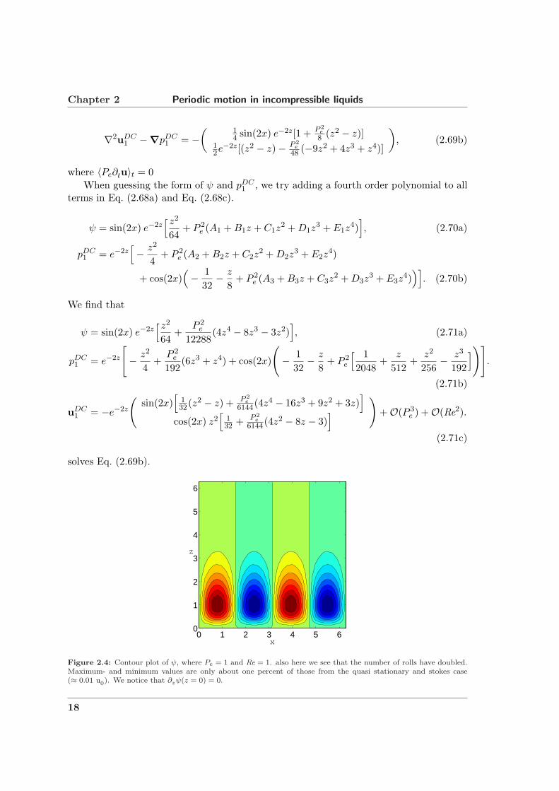
1 , we try adding a fourth order polynomial to allterms in Eq. (2.68a) and Eq. (2.68c).
ψ = sin(2x) e−2z[z2
64+ P 2
e (A1 + B1z + C1z2 + D1z
3 + E1z4)
], (2.70a)
pDC1 = e−2z
[− z2
4+ P 2
e (A2 + B2z + C2z2 + D2z
3 + E2z4)
+ cos(2x)(− 1
32− z
8+ P 2
e (A3 + B3z + C3z2 + D3z
3 + E3z4)
)]. (2.70b)
We find that
ψ = sin(2x) e−2z[z2
64+
P 2e
12288(4z4 − 8z3 − 3z2)
], (2.71a)
pDC1 = e−2z
[− z2
4+
P 2e
192(6z3 + z4) + cos(2x)
(− 1
32− z
8+ P 2
e
[ 12048
+z
512+
z2
256− z3
192
])].
(2.71b)
uDC1 = −e−2z
(sin(2x)
[132(z2 − z) + P 2
e6144(4z4 − 16z3 + 9z2 + 3z)
]
cos(2x) z2[
132 + P 2
e6144(4z2 − 8z − 3)
])
+O(P 3e ) +O(Re2).
(2.71c)
solves Eq. (2.69b).
x
z
0 1 2 3 4 5 60
1
2
3
4
5
6
Figure 2.4: Contour plot of ψ, where Pe = 1 and Re = 1. also here we see that the number of rolls have doubled.Maximum- and minimum values are only about one percent of those from the quasi stationary and stokes case(≈ 0.01 u0). We notice that ∂zψ(z = 0) = 0.
18

Comparing analytical and numerical solutions Section 2.4
2.3.3 Solution for O(P ne ) and O(Re1)
From the results in the two previous subsections we see that a solution to the time averagedEq. (2.48b)
〈∇2u1〉t − 〈∇p1〉t = 〈(u0 ·∇)u0〉t. (2.72)
can be found by time averaging
∇2uDC1 −∇pDC
1 =12
(Re[u0]·∇Re[u0] + Im[u0]·∇Im[u0]
). (2.73)
and substituting u0 by an O(Pne ) expansion of usto in Pe
usto =
(cos(x)
√1+iPe e−z
√1+iPe−e−z√
1+iPe−1
sin(x) e−z√
1+iPe−e−z
1−√1+iPe
), (2.74)
and then guessing
uDC1 =
(+∂xψn
−∂zψn
), ψn = sin(2x) e−2z
n∑
k=0,2,4...
(P k
e
k+2∑
m=2...
[akm zm
])(2.75a)
pDC1 = e−2z
[b z2 +
n∑
k=2,4...
(P k
e
k+2∑
l=3...
[ckl zl
])+ cos(2x)
n∑
k=0,2,4...
(P k
e
k+1∑
h=0...
[dkh zh
])].
(2.75b)
If these guesses are inserted into Eq. (2.73), we get two equations with a total of 4, 13,28, 49, 76, 109 unknown constants for n=0, 2, 4, 6, 8, 10, respectively .
2.4 Comparing analytical and numerical solutions
When comparing solutions, we need to establish a specific property which we want tocompare. In this section we have chosen to look at the average value of the absolutevelocity, computed in an square area adjacent to the channel wall with the same widthas the pitch between the piezo elements. The numerical calculation is performed withdimensions and the following values:
symbol value unit descriptionPπ 2π × 10−6 m Piezo pitchρ 1000 kg m−3 Fluid densityη 1× 10⁻³ Pa s Fluid viscosityPe to be chosen − Peclet numbers to be chosen, s > 1 − ConstantRe s× Pe − Reynolds numberω Pe × 106 s−1 Angular frequencyu0 s× Pe m s−1 Slip velocity
Table 2.1: The values used for the numerical simulation(see Appendix A).
19

Chapter 2 Periodic motion in incompressible liquids
By defining our values like this, we can choose any value of Pe and Re and we stillfulfill the definitions from Eq. (2.3a) and Eq. (2.3b). In order to justify our time averagingmethod we must require that Re > Pe. Hence, we set Re = s× Pe, where s is a constantlarger than 1. For different values of Pe we then compute the Average Absolute Velocity,AAV
AAV =
∫Ω |u|dxdz
P 2π
(2.76)
In Fig. 2.5 and Fig. 2.7 the AAV is plotted for increasing values of Pe for different O(Pne )-
expansions. To estimate how well these expansions correspond to the numeric result, wedefine the error,
Error =|AAVO(P n
e ) −AAVnum|AAVnum
× 100 % (2.77)
The error is plotted in Fig. 2.6 and Fig. 2.8.
0 0.5 1 1.5 210
−4
10−3
10−2
10−1
100
101
Re = 10Pe, s =10
Pe
AA
V
NumSolO(P 10
eRe1)
O(P 8eRe1)
O(P 6eRe1)
O(P 4eRe1)
O(P 2eRe1)
O(P 0eRe1)
Figure 2.5: A plot of the Average Absolute Velocity,AAV. Plotted for different expansions. For Pe < 1.5the analytical results is very close to the numerical So-lution(NumSol).
0 0.5 1 1.5 210
−2
10−1
100
101
102
103
Re = 10Pe, s =10
Pe
Err
or [%
]
O(P 10e
Re1)O(P 8
eRe1)
O(P 6eRe1)
O(P 4eRe1)
O(P 2eRe1)
Figure 2.6: A plot of the error. Plotted for differ-ent expansions. The fluctuations for O(P 6
e Re1) andO(P 10
e Re1) are caused by the sign change in the dif-ference.
20

High-order terms Section 2.5
0 0.5 1 1.5 210
−5
10−4
10−3
10−2
10−1
100
Re = 2Pe, s =2
Pe
AA
V
NumSolO(P 10
eRe1)
O(P 8eRe1)
O(P 6eRe1)
O(P 4eRe1)
O(P 2eRe1)
O(P 0eRe1)
Figure 2.7: A plot of the Average Absolute Velocity,AAV. Plotted for different expansions. Again we seethat for Pe < 1.5 the analytical results is very close tothe numerical Solution(NumSol). Notice that NumSol-values under 10−4 are uncertain, since the simulationswere conducted with a absolute tolerance of 10−4.
0 0.5 1 1.5 210
−2
10−1
100
101
102
103
Re = 2Pe, s =2
PeE
rror
[%]
O(P 10e
Re1)O(P 8
eRe1)
O(P 6eRe1)
O(P 4eRe1)
O(P 2eRe1)
Figure 2.8: A plot of the error. Plotted for differentexpansions. It can be seen that the error is especiallylarge for small values of Pe, this is a result of comparingvery small unprecise numbers.
From Fig. 2.6 and Fig. 2.8 it can be seen that all the analytic solutions are valid forPe < 1.2. For Pe > 1.2 it is only O(P 2
e Re1) and O(P 6e Re1) that are accurate, and still
these are only accurate until Pe ≈ 2. This show, as expected, that the perturbationtheory becomes invalid, for large parameters. Increased accuracy might be achieved bycalculating higher orders in Re. We attempt to do so in the following section.
2.5 High-order terms
Before we can calculate the second-order terms, we must first calculate the remainingfirst-order terms.
2.5.1 Determination of u1n and p1n
To find u1n and p1n we insert Eq. (2.57a) into Eq. (2.48b)
[∇2 − Pe∂t
](uDC
1 +∞∑
n=1
u1n
)−∇
(pDC1 +
∞∑
n=1
p1n
)= (u0 ·∇)u0, (2.78)
After separating known terms from unknown we get:
[∇2 − Pe∂t
] ∞∑
n=1
u1n −∇∞∑
n=1
p1n = (u0 ·∇)u0 + ∇pDC1 −∇2uDC
1 . (2.79)
21

Chapter 2 Periodic motion in incompressible liquids
Inserting u0, uDC1 and pDC
1 of order O(P 2e ) we get:
[∇2 − Pe∂t
] ∞∑
n=1
u1n −∇∞∑
n=1
p1n =
(Kx
Kz
)(2.80)
where
Kx =− e−2z sin(2x)1536
([384− 48P 2
e z(1 + z)]cos(2t) + 192Pez sin(2t)
)(2.81a)
Kz =− e−2z
4608
([− 2304z + 144(16z2 + 3z2P 2
e ) + 384P 2e z3 − 336P 2
e z4]cos(2t)− 48Pe(36z2 − 24z3) sin(2t)
)
(2.81b)
When looking at the terms in Eq. (2.81a) and Eq. (2.81b) we immediately see that thereare only terms proportional to sin(2t) or cos(2t). Since all operators on the left hand sideof Eq. (2.80) are linear with respect to time, t, we can conclude that
∞∑
n=1
u1n = u12,∞∑
n=1
p1n = p12. (2.82)
Hence, the equation to be solved becomes
[∇2 − Pe∂t
]u12 −∇p12 =
(Kx
Kz
)(2.83)
we find that
ψ12 = e−2z sin(2x)
(Pe
[z2
512+
z3
192
]sin(2t) +
[z2
64+ P 2
e
(− z2
2048− 5z3
3072− z4
1024
)]cos(2t)
)
(2.84)
u12 =e−2z
3072
[[96(z − z2)− P 2
e (3z + 12z2 + 2z3 − 6z4)]cos(2t) + 4 Pe(3z + 9z2 − 8z3) sin(2t)
]sin(2x)
(2.85)
w12 =e−2z
3072
[[− 96z2 + P 2e z2(3 + 10z + 6z2)
]cos(2t)− 4 Pez
2(3 + 8z) sin(2t)]
cos(2x)
(2.86)
p12 = e−2z
([− z2
4+ P 2
e
(z3
32+
7z4
192
)
22

High-order terms Section 2.5
+[− 1
32− z
8+ P 2
e
(1
512+
3z
512+
3z2
256+
z3
192
)]cos(2x)
]cos(2t)
+[− Pe z3
8− Pe
(1
253+
z
64+
z2
32
)cos(2x)
]sin(2t)
)(2.87)
solves Eq. (2.83)
2.5.2 Re to second order
After finding the full solution to u1 and p1 we can begin to look at the second orderequation Eq. (2.48c). To find uDC
2 we start with Eq. (2.48c)
O(Re2) :[∇2 − Pe∂t
]u2 −∇p2 = (u1 ·∇)u0 + (u0 ·∇)u1. (2.88)
We start by looking at the term (u1 ·∇)u0
(u1 ·∇)u0 =∞∑
n=0
(u1n∂x + w1n∂z
)(Re[u0] cos(t)− Im[u0] sin(t)
). (2.89)
When time averaging these terms we get
n = 0, 〈(uDC1 ·∇)u0〉t = 0
n = 1, 〈(u11 ·∇)u0〉t =12
(a11x∂xRe[u0] + a11z∂zRe[u0]
)− 1
2
(b11x∂xIm[u0] + b11z∂zIm[u0]
)= 0
n > 1, 〈(u1n ·∇)u0〉t = 0. (2.90)
Since a1 = 0 and b1 = 0 according to Eq. (2.82)Hence 〈(u1 ·∇)u0〉t = 0. Next we look at the term (u0 ·∇)u1
(u0·∇)u1 =(Re[u0] cos(t)∂x − Im[u0] sin(t)∂x + Re[w0] cos(t)∂z − Im[w0] sin(t)∂z
) ∞∑
n=0
u1n
(2.91)When time averaging these terms we get
n = 0, 〈(u0 ·∇)uDC1 〉t = 0
n = 1, 〈(u0 ·∇)u11〉t =12
(Re[u0]∂xa11 + Re[w0]∂za11
)− 1
2
(Im[u0]∂xb11 + Im[w0]∂zb11
)= 0
n > 1, 〈(u0 ·∇)u1n〉t = 0. (2.92)
Hence (u0 ·∇)u1 = 0. Finally we look at the time average of the entire equation.
〈O(Re2)〉t = ∇2uDC2 −∇pDC
2 = 0 (2.93)
It is obvious that uDC2 = 0 and pDC
2 = 0 fulfill Eq. (2.93). However, this result does nothelp to increase the precision of uDC . Hence, we must attempt to calculate uDC
3
23
Chapter 2 Periodic motion in incompressible liquids
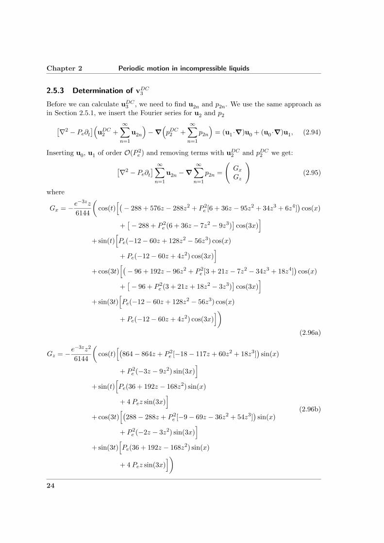
2.5.3 Determination of vDC3
Before we can calculate uDC3 , we need to find u2n and p2n. We use the same approach as
in Section 2.5.1, we insert the Fourier series for u2 and p2
[∇2 − Pe∂t
](uDC
2 +∞∑
n=1
u2n
)−∇
(pDC2 +
∞∑
n=1
p2n
)= (u1 ·∇)u0 + (u0 ·∇)u1, (2.94)
Inserting u0, u1 of order O(P 2e ) and removing terms with uDC
2 and pDC2 we get:
[∇2 − Pe∂t
] ∞∑
n=1
u2n −∇∞∑
n=1
p2n =
(Gx
Gz
)(2.95)
where
Gx = −e−3zz
6144
(cos(t)
[(− 288 + 576z − 288z2 + P 2e [6 + 36z − 95z2 + 34z3 + 6z4]
)cos(x)
+[− 288 + P 2
e (6 + 36z − 7z2 − 9z3)]cos(3x)
]
+sin(t)[Pe(−12− 60z + 128z2 − 56z3) cos(x)
+ Pe(−12− 60z + 4z2) cos(3x)]
+cos(3t)[(− 96 + 192z − 96z2 + P 2
e [3 + 21z − 7z2 − 34z3 + 18z4])cos(x)
+[− 96 + P 2
e (3 + 21z + 18z2 − 3z3)]cos(3x)
]
+sin(3t)[Pe(−12− 60z + 128z2 − 56z3) cos(x)
+ Pe(−12− 60z + 4z2) cos(3x)])
(2.96a)
Gz = −e−3zz2
6144
(cos(t)
[(864− 864z + P 2
e [−18− 117z + 60z2 + 18z3])sin(x)
+ P 2e (−3z − 9z2) sin(3x)
]
+sin(t)[Pe(36 + 192z − 168z2) sin(x)
+ 4 Pez sin(3x)]
+cos(3t)[(
288− 288z + P 2e [−9− 69z − 36z2 + 54z3]
)sin(x)
+ P 2e (−2z − 3z2) sin(3x)
]
+sin(3t)[Pe(36 + 192z − 168z2) sin(x)
+ 4 Pez sin(3x)])
(2.96b)
24

Concluding remarks Section 2.6
When looking at the terms in Eq. (2.96a) and Eq. (2.96b) we immediately see that thereare only terms proportional to cos(t), sin(t), cos(3t) and sin(3t). Hence, we conclude that
∞∑
n=1
u2n = u21 + u23,∞∑
n=1
p2n = p21 + p23. (2.97)
Hence, the equation to be solved becomes
[∇2 − Pe∂t
](u21 + u23)−∇(p21 + p23) =
(Gx
Gz
). (2.98)
Fortunately this equation can be split up into two simpler equations
[∇2 − Pe∂t
]u21 −∇p21 =
(Gx ∝
[sin(t) ∨ cos(t)
]
Gz ∝[sin(t) ∨ cos(t)
])
, (2.99a)
[∇2 − Pe∂t
]u23 −∇p23 =
(Gx ∝
[sin(3t) ∨ cos(3t)
]
Gz ∝[sin(3t) ∨ cos(3t)
])
. (2.99b)
where Gx ∝[sin(t)∨cos(t)
]means the terms in Gx which depends on either sin(t) or cos(t).
Unfortunately these two equations becomes rather cumbersome and since the contributionfrom uDC
3 to uDC is very small we will not attempt to solve them. In a real physical setupwe cannot choose the value of u0 as freely as done in Section 2.4. u0 will be given by theproduct of the frequency and the amplitude of the piezo oscillations, Aπ. Hence, if thefrequency is 1 MHz and Aπ is 1 nm, then u0 = 1× 10⁻³ m/s. This means that for a waterfilled system with k = 2π
10 µm we have a Reynolds number, Re = 0.01. Remembering thepre-factor to uDC
3 is Re3 = 10−6, it is clear that uDC3 is of less importance. Therefore we
must settle with the results from Section 2.4.
2.6 Concluding remarks
Even though the results from Section 2.4 becomes unprecise for large parameters(as theperturbation-method breaks down), they are sufficient to reveal that an oscillating bound-ary alone, only effects the very nearest part of the incompressible liquid and that theinduced motion dies very rapidly as the distance to the wall becomes larger. Hence, wecan not explain the acoustic radiation force and acoustic streaming patterns far from theboundary. We are forced to discard the incompressible-liquid-model.
25


Chapter 3
Sound absorption in compressible liquids
As it has been shown in Chapter 2 we cannot explain the effects of streaming and focusing,simply by an incompressible liquid surrounded by oscillating walls. So in our next attemptwe will treat the liquid as compressible, and under the influence of sound waves.
3.1 Acoustic perturbation theory
To describe the absorption of sound in a compressible liquid in the domain Ω, we needthe three fundamental equations; the continuity equation (Eq. (3.1)), the Navier-Stokesequation (Eq. (3.2)), and an equation of state (Eq. (3.3)).
∂tρ + ∇·(ρu) = 0, u ≡ (uex, vey, wez) (3.1)
ρ[∂tu + (u·∇)u
]= −∇p + η∇2u + βη∇
(∇·u
), (3.2)
p = f(ρ). (3.3)
where
β ≡ 13
+ζ
η. (3.4)
According to Stoke’s viscosity relation ζ = 4η/3 [31], the numerical value of β is thereforeβ = 5/3. We notice that for compressible fluids the normal no-slip boundary conditionchanges from velocity u(∂Ω) to flux J(∂Ω)
u(∂Ω, t) = 0 =⇒ J(∂Ω, t) = 0. (3.5)
Since velocities and fluctuations are expected to be small we assume the followingapproximations to be valid.
p = p0 + p1 + p2 + . . . , (3.6a)ρ = ρ0 + ρ1 + ρ2 + . . . , (3.6b)u = 0 + u1 + u2 + . . . . (3.6c)
27

Chapter 3 Sound absorption in compressible liquids
Where the subscript indicates the order of the term. The EOS is found from the expansion
p(ρ0 + [ρ1 + ρ2]) = p(ρ0) +∂p
∂ρ(ρ1 + ρ2) +
∂2p
∂ρ2(ρ1 + ρ2)
2 . . . (3.7)
wherec20 ≡
∂p
∂ρ(3.8)
and to reduce the complexity of the equations, we assume that
∂2p
∂ρ2= 0. (3.9)
3.2 The non-viscous case
To reduce the complexity of the equations we assume that η = 0 and ζ = 0.
3.2.1 Zeroth-order perturbation
The zeroth-order equations becomes
∂tρ0 = 0, (3.10)
∇p0 = 0, (3.11)
p0 = p(ρ0). (3.12)
From Eq. (3.12) we see that p0 is a function of ρ0. Hence from Eqs. (3.10) and (3.11) itcan be seen that ρ0 as well as p0 is constant in both time and space. ρ0 and p0 can bethought of as the equilibrium or background density and pressure when no sound field ispresent. Notice, we have in Eq. (3.6c) already assumed the velocity to be zero when nosound field is present.
3.2.2 First-order perturbation
The first-order equations becomes
∂tρ1 + ∇·(ρ0u1) = 0, (3.13)
ρ0∂tu1 = −∇p1, (3.14)
p1 = c20ρ1. (3.15)
Taking the divergence of Eq. (3.14) and inserting Eq. (3.13) and Eq. (3.15) we get
∂2t ρ1 = c2
0∇2ρ1. (3.16)
Taking the time derivative of Eq. (3.13) and inserting Eq. (3.14) and Eq. (3.15) we get
∂2t p1 = c2
0∇2p1. (3.17)
28

The non-viscous case Section 3.2
By inserting Eq. (3.15) into Eq. (3.14) and taking the time derivative, and then insertingEq. (3.13) we get
∂2t u1 = c2
0∇(∇·u1). (3.18)
However, as η = 0 we may assume that u1 is irrotational and can therefore be defined bya scalar potential
u1 = ∇ϕ1. (3.19)
since u1 is irrotational (∂iuj = ∂jui), we make use of ∇(∇·u) = ∇·(∇u) = ∇2u
∇(∇·u) = ∂i∂juj = ∂j∂iuj = ∂j∂jui = ∇2u, (3.20)
∇·(∇u) = ∂i∂iuj = ∇2u, (3.21)
to rewrite Eq. (3.18) to a wave equation. Hence, we got
∂2t u1 = c2
0∇2u1. (3.22)
Since Eqs. (3.16 - 3.17) and Eq. (3.22) all are standard wave equations, they have solutionsconsisting of linear combinations of traveling waves (Aei[k0x−ωt] + Bei[−k0x−ωt] in the 1Dcase). This indicates that the sound wave propagating in the liquid is described by thefirst order terms (u1, p1, ρ1).
By inserting Eq. (3.19) and Eq. (3.15) into Eq. (3.14) and removing ∂x, ∂y, ∂z by meansof integration, we can express ρ1 by ϕ1
ρ1 = −ρ0
c20
∂tϕ1. (3.23)
By inserting Eq. (3.23) into Eq. (3.15) we get
p1 = −ρ0∂tϕ1. (3.24)
By inserting Eq. (3.19) and Eq. (3.23) into Eq. (3.13) we immediately see that ϕ1 alsofollows the wave equation
∂2t ϕ1 = c2
0∇2ϕ1. (3.25)
By inserting a plane harmonic wave, ρ1 = ρ1ei(k0x−ωt), k0 = ω/c0 into Eq. (3.23) or
Eq. (3.24) and combining with Eq. (3.19) we can find u1(ρ1) or u1(p1)
u1 =c0
ρ0
ρ1ex =c20
Zρ1ex, (3.26)
u1 =1
c0ρ0
p1ex =1Z
p1ex, (3.27)
where Z = ρ0c0 is the acoustic impedance.
29

Chapter 3 Sound absorption in compressible liquids
3.2.3 Second-order perturbation
The governing equations to second order becomes,
∂tρ2 + ∇·(ρ0u2) + ∇·(ρ1u1) = 0, (3.28)
ρ0∂tu2 + ρ1∂tu1 + ρ0(u1 ·∇)u1 = −∇p2, (3.29)
p2 = c20ρ2. (3.30)
Introducing the mass-fluxJ2 ≡ ρ0u2 + ρ1u1, (3.31)
we can write Eq. (3.28) as∂tρ2 + ∇·J2 = 0. (3.32)
Inserting both Eq. (3.31) and Eq. (3.30) into Eq. (3.29) we get
∂tJ2 = −F− c20∇ρ2, (3.33)
whereF ≡ ρ0(u1 ·∇)u1 + ρ0u1(∇·u1). (3.34)
In the definition of F, we have used Eq. (3.13) to rewrite u1∂tρ1 = −u1∇·(ρ0u1). Takingthe time average of Eq. (3.32) and Eq. (3.33) we get
∇·J′′2 = 0 ⇒ ∇·u′′2 = − 1ρ0
∇·〈ρ1u1〉t. (3.35)
∇ρ′′2 = − 1c20
F′′, (3.36)
where J′′2 = 〈J2〉t and
〈ρ1u1〉t =12
(Re[ρ1]Re[u1] + Im[ρ1]Im[u1]
)=
12Re [ρ1u
∗], (3.37)
F′′ =12ρ0
[(Re
[u1
]·∇)Re
[u1
]+
(Im
[u1
]·∇)Im
[u1
]]
+12ρ0
[Re
[u1
](∇·Re[u1
])+ Im
[u1
](∇·Im[u1
])]
=12ρ0Re
[(u1 ·∇)u∗1
]+
12ρ0Re
[u1(∇·u∗1
]. (3.38)
From these equations we see to our surprise that Eq. (3.35) and Eq. (3.36) no longerpredicts a relation between u′′2 and ρ′′2. Hence they cannot be solved for a general case. Thisshows us that the approximation of neglecting the viscosity is a far to rough approximation.We can therefore conclude that viscosity must be included.
30

The viscous case Section 3.3
3.3 The viscous case
In this section we assume that η 6= 0 and ζ 6= 0.
3.3.1 Zeroth-order perturbation
Same as without viscosity. Again ρ0 and p0 are constant in time and space, and u0 = 0.
3.3.2 First-order perturbation
The first order equations becomes
−∂tρ1 = ∇·(ρ0u1) = ρ0(∇·u1), (3.39)
ρ0∂tu1 = −∇p1 + η∇2u1 + βη∇(∇·u1
), (3.40)
p1 = c20ρ1. (3.41)
Taking the divergence of Eq. (3.40) and inserting the left hand side of Eq. (3.39) we find
∂2t ρ1 = c2
0∇2ρ1 + (β + 1)η
ρ0
∇2∂tρ1 (3.42)
by insertion of Eq. (3.41) we get
∂2t p1 = c2
0∇2p1 + (β + 1)η
ρ0
∇2∂tp1. (3.43)
In the non-stationary steady state, we may assume that ρ1, p1 and u1 are oscillatingharmonically in time, since the system is driven by a harmonic force, f(r, t) = f(r)e−iωt.Hence, we introduce
ρ1 = ρ1e−iωt, p1 = p1e
−iωt, u1 = u1e−iωt. (3.44)
which allows us to substitute
∂t = −iω and ∂2t = −ω2 (3.45)
into Eq. (3.43), which yields[1− i
ωη(β + 1)ρ0c
20
]∇2p1 +
ω2
c20
p1 = 0. (3.46)
Furthermore we find the relation between p1 and u1 by inserting Eq. (3.39) into Eq. (3.40)and then substitute the time derivatives as defined.
∇2u1 = −iωρ0
ηu1 +
[1− i
ωβη
ρ0c20
]1η∇p1 (3.47)
31

Chapter 3 Sound absorption in compressible liquids
These are the equations describing the first-order pressure field and particle velocity. No-tice that the particle velocity is the velocity at which a particle oscillates and not at whichthe wave travels.
We can extract further information from Eq. (3.46), if we rewrite it using the firstorder Taylor expansion, (1− x)p ≈ 1− px
∇2p1 = −ω2
c20
[1 + i
ωη(β + 1)ρ0c
20
]p1. (3.48)
The term (β+1)ωη2ρ0c20
has a typical numerical value of
γ ≡ (β + 1)ωη
2ρ0c20
≈ 106 s−1 × 10⁻³ Pa s103 kg m−3 × 10⁶ m2 s−2
≈ 10−6. (3.49)
Hence, we can argue that
[1 + i
ωη(β + 1)ρ0c
20
]≈
[1 + iγ
]2. (3.50)
Our Helmholtz equation then becomes
∇2p1 = −k20
[1 + iγ
]2p1 , k0 ≡
ω
c0
. (3.51)
From simple insertion, we se that the plane attenuated wave,
p1 = p1e±ik0(1+iγ)x = p1e
±k0(i−γ)x, (3.52)
is a solution to the Helmholtz equation.By inserting the plane attenuated wave into Eq. (3.39), we see that
∇·u1 = − 1ρ0
∂tρ1 =iω
ρ0
ρ1ek0(i−γ)x−iωt. (3.53)
Hence,
u1 =(1− iγ)c0
ρ0
ρ1ex =(1− iγ)c2
0
Zρ1ex (3.54)
fulfills the equation. We find u1(p1) by inserting ρ1 = p1/c20 into Eq. (3.54)
u1 =(1− iγ)
c0ρ0
p1ex =(1− iγ)
Zp1ex (3.55)
Notice that if γ → 0 Eq. (3.54) and Eq. (3.55) are identical to Eq. (3.26) and Eq. (3.27).
32

The viscous case Section 3.3
3.3.3 Second-order perturbation
The second order equations becomes
∂tρ2 + ∇·(ρ0u2) + ∇·(ρ1u1) = 0, (3.56)
ρ0∂tu2 + ρ1∂tu1 + ρ0(u1 ·∇)u1 = −∇p2 + η∇2u2 + βη∇(∇·u2
), (3.57)
p2 = c20ρ2. (3.58)
Inserting J2 and F as previously defined we get
∂tρ2 + ∇·J2 = 0, (3.59)
∂tJ2 = −F−∇p2 + η∇2u2 + βη∇(∇·u2
). (3.60)
Taking the time average of Eq. (3.59) and Eq. (3.60) we find
∇·J′′2 = 0
∇·u′′2 = − 1ρ0
∇·〈ρ1u1〉t = − 1c20ρ0
∇·〈p1u1〉t = − 12c2
0ρ0
∇·Re[p1u
∗1
]
∇·u′′2 = S, S = − 12c2
0ρ0
∇·Re[p1u
∗1
](3.61)
0 =− F′′ −∇p′′2 + η∇2u′′2 + βη∇(∇·u′′2
)
η∇2u′′2 + βη∇(∇·u′′2
)=∇p′′2 + F′′, (3.62)
We notice that 〈∂tJ2〉t = 0 in steady state. Hence, to find the streaming velocity, u′′2, weneed to solve a scalar equation and a vector equation where both S and F′′ consists onlyof known terms. We notice that if u′′2 is solenoidal, then Eq. (3.62) is identical to that ofNyborg[26]. In Chapter 7 we shall solve these equations for three different examples. Butfirst we will look closer at the first-order terms, which contains the acoustic waves.
33

Chapter 4
Planer sound waves
As shown in Section 3.2.2 the acoustic waves is introduced in the first-order equation,which show up to be ordinary wave-equations. In this chapter we shall look closer at thesolutions to the wave-equation.
4.1 Wave-emission from an oscillating wall
We imagine a semi-infinite fluid next to a piezo crystal located such that the fluid-crystalinterface is at (x, y, z) = 0 with the outwards pointing normal vector, n. The crystal isset to vibrate and the position, dw(t) is thus described by dw(t) = i`ne−iωt, where ` isthe vibration amplitude. The velocity of the wall, uw and the acceleration, aw is foundby single and double differentiation, respectively.
uw = u1(0, t) = `ωne−iωt. (4.1)
aw = ∂tu1(0, t) = −i`ω2ne−iωt. (4.2)
Assuming the wall has vibrated long enough for a steady state to be established, we see,by using uw as a boundary condition, that the first order velocity of the fluid can bedescribed as
u1(r, t) = `ωnei(k·r−ωt), (4.3)
where k = k0n|n| . By requiring that c0 = ω/k0 we ensure that u1 fulfills the wave equation.
Using Eqs. (3.19 - 3.24) we find ϕ, ρ1 and p1
ϕ(r, t) =− i`c0ei(k·r−ωt), (4.4a)
ρ1(r, t) =ρ0`k0ei(k·r−ωt), (4.4b)
p1(r, t) =ρ0ω`c0ei(k·r−ωt) = Z0ω`ei(k·r−ωt). (4.4c)
where Z0 = ρ0c0 is the acoustic impedance of the media.
35

Chapter 4 Planer sound waves
4.2 Wave propagation through a single interface
An unattenuated sound wave traveling (from left to right, hence, the subscript r) in onemedia(A), is eventually bound to hit the interface of another media(B). At such an interfacethe incoming sound wave, ϕA,r, will be split into a reflected, ϕA,l, and a transmitted, ϕB,r,wave. Hence, we got
A B
part
icle
vel
oci
ty
uA,r
uB,r
uA,l
uA
Figure 4.1: Since ϕ is not continues overinterfaces we plot the particle velocity. Theincoming wave, uA,r is split up into a re-flected wave, uA,l and a transmitted wave,uB,r.
ϕA(x, t) =Arei(kAx−ωt) + Ale
i(−kAx−ωt), (4.5a)
ϕB(x, t) =Brei(kBx−ωt) + 0ei(−kBx−ωt). (4.5b)
To describe the amplitudes of the resulting waves, Al and Br, we define the reflec-tion coefficient, RI and the transmission coefficient, TI , so they represent the ratio be-tween the reflected or transmitted intensity and that of the incoming wave (IA,r(L, t) =〈ZA(∂xϕA,r)
2〉t). The subscript ’I’ reminds us that the coefficients apply to the intensity.Let the interface be positioned at x = L, then due to conservation of energy we must
require that
IA,r(L, t) =IA,l(L, t) + IB,r(L, t), (4.6a)
〈ZA(∂xϕA,r)2〉t =〈ZA(∂xϕA,l)
2〉t + 〈ZB(∂xϕB,r)2〉t, (4.6b)
−12ZAk2
A|Ar|2 =− 12ZAk2
A|Al|2 − 12ZBk2
B|Br|2, (4.6c)
1 =
(|Al||Ar|
)2
+ρBkB
ρAkA
(|Br||Ar|
)2
, (4.6d)
where we have used Zi = ρici = ρiω/ki. Hence, we define
RI =
(|Al||Ar|
)2
, (4.7a)
TI =ρBkB
ρAkA
(|Br||Ar|
)2
, (4.7b)
so that RI + TI = 1.
36

Wave propagation through a single interface Section 4.3
To determine the the amplitudes of Al and Br we need two equations, which we derivefrom boundary conditions.
By requiring that the particle velocity, u is continues over the interface we get theboundary condition ∂xϕA(L, t) = ∂xϕB(L, t). And from Newton’s third law we know thatthe force on the interface must be equal on both sides, hence, the same must be validfor the pressure, leading us to the another boundary condition: ρAϕA(L, t) = ρBϕB(L, t).Hence we got the two equations
ikAArei(kAL−ωt) − ikAAle
i(−kAL−ωt) =ikBBrei(kBL−ωt), (4.8a)
ρAArei(kAL−ωt) + ρAAle
i(−kAL−ωt) =ρBBrei(kBL−ωt), (4.8b)
which can be reduced to
kA
kB
AreikAL − kA
kB
Ale−ikAL =Bre
ikBL, (4.9a)
ρA
ρB
AreikAL +
ρA
ρB
Ale−ikAL =Bre
ikBL, (4.9b)
by inserting one into the other we see that
Al
Ar=
ZB − ZA
ZB + ZA
ei2kAL. (4.10)
Dividing Eq. (4.9b) by Ar and inserting Eq. (4.10) we get
Br
Ar=
ρA
ρB
(2ZB
ZB + ZA
)ei(kA−kB)L. (4.11)
From Eq. (4.10) and Eq. (4.11) we see that
RI(A → B) =
(|Al||Ar|
)2
=
(ZB − ZA
ZB + ZA
)2
, (4.12a)
TI(A → B) =ρBkB
ρAkA
(|Br||Ar|
)2
=ρBkB
ρAkA
[ρA
ρB
(2ZB
ZB + ZA
)]2
=ZA
ZB
(2ZB
ZB + ZA
)2
. (4.12b)
To verify this result, we check that intensity is conserved
1 =RI + TI ,
1 =
(ZB − ZA
ZB + ZA
)2
+ZA
ZB
(2ZB
ZB + ZA
)2
,
1 =Z2
B + Z2A − 2ZBZA
(ZB + ZA)2+
4ZBZA
(ZB + ZA)2,
1 =(ZB + ZA)2
(ZB + ZA)2= 1. (4.13)
37

Chapter 4 Planer sound waves
4.3 Wave propagation through multiple interfaces
When the acoustic wave passes through several interfaces the corresponding equations getsslightly more complicated. we have four materials(A, B, C, D) divided by three interfacesat x = LA, x = LB and x = LC as shown in Fig. 4.2.
A B C D
LA LB LC
part
icle
vel
oci
ty
u
Figure 4.2: The incoming wave, ur ispropagated through several interfaces.
ϕA(x, t) =Arei(kAx−ωt) + Ale
i(−kAx−ωt), (4.14a)
ϕB(x, t) =Brei(kBx−ωt) + Ble
i(−kBx−ωt), (4.14b)
ϕC(x, t) =Crei(kCx−ωt) + Cle
i(−kCx−ωt), (4.14c)
ϕD(x, t) =Drei(kDx−ωt) + Dle
i(−kDx−ωt), (4.14d)
From the two boundary conditions
∂xϕj+1(Lj , t) =∂xϕj(Lj , t), (4.15)−ρj+1∂tϕj+1(Lj , t) =− ρj∂tϕj(Lj , t), (4.16)
we got the two equations
ikj+1ϕ∗j+1,re
i(kj+1Lj−ωt) − ikj+1ϕ∗j+1,re
i(−kj+1Lj−ωt) =ikjϕ∗j,re
i(kjLj−ωt) − ikjϕ∗j,le
i(−kjLj−ωt)
(4.17a)
iρj+1ωϕ∗j+1,rei(kj+1Lj−ωt) + iρj+1ωϕ∗j+1,re
i(−kj+1Lj−ωt) =iρjωϕ∗j,rei(kjLj−ωt) + iρjωϕ∗j,le
i(−kjLj−ωt).
(4.17b)
Which we can reduce and write as matrix equation
eikj+1Lj −e−ikj+1Lj
eikj+1Lj e−ikj+1Lj
ϕ∗j+1,r
ϕ∗j+1,l
=
kj
kj+1eikjLj − kj
kj+1e−ikjLj
ρj
ρj+1eikjLj
ρj
ρj+1e−ikjLj
ϕ∗j,r
ϕ∗j,l
(4.18a)
We then use the relation[a bc d
]−1
=1
ad− cd
[d −b−c a
], (4.19)
to multiply both sides by the inverse of the left matrix.
ϕ∗j+1,r
ϕ∗j+1,l
=
12
e−ikj+1Lj e−ikj+1Lj
−eikj+1Lj eikj+1Lj
kj
kj+1eikjLj − kj
kj+1e−ikjLj
ρj
ρj+1eikjLj
ρj
ρj+1e−ikjLj
ϕ∗j,r
ϕ∗j,l
(4.20a)
38

Wave propagation through multiple interfaces Section 4.3
ϕ∗j+1,r
ϕ∗j+1,l
=
12
(kj
kj+1+
ρj
ρj+1
)ei(kj−kj+1)Lj
(ρj
ρj+1− kj
kj+1
)e−i(kj+kj+1)Lj
(ρj
ρj+1− kj
kj+1
)ei(kj+kj+1)Lj
(kj
kj+1+
ρj
ρj+1
)e−i(kj−kj+1)Lj
ϕ∗j,r
ϕ∗j,l
(4.20b)
By introducing the transmission matrix
T(j+1,j) =
12
(kj
kj+1+
ρj
ρj+1
)ei(kj−kj+1)Lj 1
2
(ρj
ρj+1− kj
kj+1
)e−i(kj+kj+1)Lj
12
(ρj
ρj+1− kj
kj+1
)ei(kj+kj+1)Lj 1
2
(kj
kj+1+
ρj
ρj+1
)e−i(kj−kj+1)Lj
, (4.21)
the equation simplifies to ϕ∗j+1,r
ϕ∗j+1,l
= T(j+1,j)
ϕ∗j,r
ϕ∗j,l
. (4.22)
The transmission matrix can be use multiple times with changing indexes, to find ϕN
ϕ∗N,r
ϕ∗N,l
= T(N,N−1)T(N−1,N−2) . . . T(2,1)
ϕ∗1,r
ϕ∗1,l
(4.23)
Assuming a piezo electric element is located at x = 0 is vibrating with the angular fre-quency, ω, and the amplitude, `. We find the particle velocity at the to be
uw = ∂xϕA(0, t) = `ωe−iωt. (4.24)
We use this equation to find a relation between Ar and Al.
uw =∂xϕA(x, t), x = 0 (4.25a)
uw =ikA
(Are
ikAx −Ale−ikAx
)e−iωt, x = 0 (4.25b)
Al =Are2ikAx + i`cAeikAx, x = 0 (4.25c)
Furthermore we assume the last media stretches towards infinity. Hence, no wave is everreflected in this media. This is a quite good approximation to the several meters of airnormally surrounding a micro system in the lab. In the case of four medias as in Fig. 4.2we require
Dl = 0. (4.26)
By inserting Eq. (4.25c) and Eq. (4.26) into Eq. (4.23) it becomesDr
0
= T(D,C)T(C,B)T(B,A)
Ar
Ar + i`cA
. (4.27)
We have now reduced the problem to two equations with two unknowns(Ar, Dr), which isstraight forward to solve. Once Ar and Dr has been found, Al is found using Eq. (4.25c).
39

Chapter 4 Planer sound waves
When we know both Ar and Al we can find Br and Bl fromBr
Bl
= T(B,A)
Ar
Al
. (4.28)
This procedure is repeated until all unknown amplitudes has been found.We apply this calculation on the one dimensional sandwich structure from Fig. 4.2,
and define domain A as consisting of silicon with a thickness of LA = 300µm, and domainB as 200 µm water and domain C as 500 µm pyrex and finally domain D as normal air.The incoming wave is generated by a piezo element located adjacent to domain A. Thissetup is similar to the one described in Section 1.3. The piezo element is set to oscillatewith an amplitude of 1 nm. Below, the pressure and particle velocity has been plotted fortwo different frequencies.
A B C D
LA LB LC
0
1
−1
Pre
ssure
×10
5[P
a]
A B C D
LA LB LC
0
1
−1
Par
ticl
eve
loci
ty[u
w]
A B C D
LA LB LC
0
1
−1Pre
ssure
×10
10[P
a] A B C D
LA LB LC
1
0
−1
Par
ticl
eve
loci
ty[u
w×
105]
o
(a) (b)
(c) (d)
Figure 4.3: Panel (a) and (b) shows the pressure p1 and particle velocity u1 for the randomly picked non-resonancefrequency 2.26 MHz. We notice the pressure is far to high for the perturbation method to be valid. This is due tothe lack of damping. Panel (c) and (d) shows the pressure p1 and particle velocity for the resonance frequency 3.56MHz. We notice the amplitude for both pressure and particle velocity has increased dramatically for the resonancefrequency.
Due to the resonance frequency the amplitudes of both the pressure and particle veloc-ity has increased dramatically. If the resonance had been exactly hit, the amplitude wouldbecome infinite. We look closer into the resonance phenomenon in Section 4.4. In orderto calculate the pressure distribution in more than one dimensions use a numerical tool
40

Acoustic Resonances Section 4.4
embedded in the commercial finite element program, COMSOL, this method is describedin Chapter 5.
4.4 Acoustic Resonances
So far we have only considered one oscillating wall, and the waves induced by it. In thissection we look at one-dimensional system bounded by two oscillating walls. The walls arelocated at x = ±L and are assumed to oscillated in opposite directions. Hence, to modelthe oscillating walls, we state
J1(±L, t) = ±ρ0ω`e−iωt, (4.29)
4.4.1 Unattenuated waves
In the case of unattenuated waves, the first order velocity field, u1 must be defined as alinear combination of two opposite travelling waves
u1(x, t) = u1(x) e−iωt, u1(x) = u1e−ik0x + Beik0x. (4.30)
However, due to the anti-symmetrically oscillating walls we must require that
u1(x) =− u1(−x)
u1e−k0(i−γ)x + Bek0(i−γ)x =− u1e
k0(i−γ)x −Be−k0(i−γ)x
u1 =−B (4.31)
Hence, u1(x) gets the form
u1(x) =u1
(e−ik0x − eik0x
)= −i2u1 sin(k0x) (4.32)
From the antisymmetry we have the boundary conditions
u1(−L) = −ω`, u1(0) = 0, u1(L) = ω`. (4.33)
To tune in to a resonance frequency we choose
k0 =nπ
L, n = 1, 2, 3... (4.34)
From the boundary conditions (x = ±L) we get
−i2u1 sin(±nπ) = ±ω`
u1 =±iω`
2 sin(±nπ)= i∞. (4.35)
This result implies that at a resonance the unattenuated wave should have an infinitely highcomplex amplitude, and consequently contain an infinitely amount of energy. This is ofcause non-physical, but so is the unattenuated waves. We therefore repeat the calculationwith attenuated waves.
41

Chapter 4 Planer sound waves
4.4.2 Attenuated waves
For attenuated waves, the first order velocity field, u1 must be a linear combination of twoopposite attenuated traveling waves
u1(x, t) = u1(x) e−iωt, u1(x) = u1e−k0(i−γ)x + Bek0(i−γ)x. (4.36)
Again, due to the antisymmetric oscillating walls, we require that u1(x) = −u1(−x), sou1 = −B. Hence, u1(x) gets the form
u1(x) =u1
(e−k0(i−γ)x − ek0(i−γ)x
)≈ u1
(2k0γx cos(k0x)− i2 sin(k0x)
)(4.37)
where we have used the fact that γ ¿ 1 ⇒ eγx ≈ (1 + γx). It is worth noting that thesmall cosine wave is non-zero at boundary, while the much larger sine wave is zero andtherefore contained in the specific region.
We still have the same boundary conditions and the resonance definition of k0
u1(−L) = −ω`, u1(0) = 0, u1(L) = ω`. (4.38)
k0 =nπ
L, n = 1, 2, 3... (4.39)
So to fulfil the boundary conditions (x = ±L) we require
u1
(± 2nπγ cos(nπ)− i2 sin(±nπ)
)= ±ω`
u1 =(−1)nω`
2nπγ. (4.40)
We notice that for attenuated waves (γ > 0) the resonance-amplitude becomes finite.However, due to the often very low value of γ, the resonance-amplitude can still be muchhigher than the wall oscillation amplitude. For n = 3 and L = 1 mm we find that
u1 ≈ −87 m/s. (4.41)
42
Chapter 5
Numerical simulations in COMSOL
In this chapter we will describe how the tools embedded in COMSOL has been used tosimulate acoustic fields. COMSOL is a commercial software package used for numericalsimulations of various physical problems. COMSOL utilizes the finite element method. Inthis chapter we shall first look at the embedded acoustic module, and secondly look athow equations can be entered manually.
5.1 The Acoustic module in COMSOL
In this section we examine the two different solving methods, which are embedded in theacoustic module. First we look at the eigenfrequency solver, which is used to find thedifferent resonance frequencies, and secondly at the time harmonic solver, which can findthe pressure field for any specified frequency.
5.1.1 The eigenfrequency solver
To find the eigenvalues of a system defined by a wave equation, the wave equation is refor-mulated to the Helmholtz equation. From Section 3.2.2 we have the first order pressure,p1, described by a standard three dimensional wave equation Eq. (3.17).
∂2t p1 = c2
0∇2p1, p1 = p1(x, y, z, t). (5.1)
Moving all terms to the left hand side and dividing by ρ0c20,
− 1ρ0
∇2p1+1
ρ0c20
∂2t p1 = 0. (5.2)
Since we only care for the steady state, we require that the solution must be periodic intime. Hence, it is required that p1 has the form,
p1(x, y, z, t) = p1(x, y, z)e−iωt. (5.3)
Inserting this into Eq. (5.2)
− 1ρ0
∇2p1e−iωt+
1ρ0c
20
∂2t p1e
−iωt = 0. (5.4)
43
Chapter 5 Numerical simulations in COMSOL
Differentiating twice with respect to time,
− 1ρ0
∇2p1e−iωt+
(−iω)2
ρ0c20
p1e−iωt = 0. (5.5)
Reinserting p1, and introducing1 λe = ω2,
− 1ρ0
∇2p1 −λe
ρ0c20
p1 = 0 (5.6)
If substituting λe
ρ0c20= k this equation is called the Helmholtz equation. The Helmholtz
equation can easily be solved analytically for very simple geometries[32]. For a box withthe side-lengths a, b and c we get
λe = c2sπ
2
(n2
a2+
m2
b2+
l2
c2
)(5.7)
where
0 < x < a , n = 1, 2, ...
0 < y < b , m = 1, 2, ... (5.8)0 < z < c , l = 1, 2, ...
For more complex geometries we use COMSOL to solve the problem numerically.
5.1.2 Example: Pseudo-one-dimensional
An example of a more complicated geometry could be blocks of different materials stackedtogether. Due to the differences in materiel parameters the solution will no longer betrivial. For further comparing, we choose to work on a pseudo one dimensional problem.By choosing a one dimensional problem, we can verify the numerical results by comparingwith analytical results based on the equations from Section 4.3. The reason why we callthis problem ’pseudo one dimensional’ is that it really is two dimensional. But we keepone dimension so narrow that, no wave can appear here, except for very high frequencies.This mean that for relative low frequencies the model can be regarded as one dimensional.Instead of setting up the problem in the COMSOL GUI we will use scripting. The problemwe are going to solve resembles the sandwich structure from Section 4.3 and Section 1.3.We start by initiating the variables we are going to use.
COMSOL1 % Initializing
2 flclear fem
3 MF = 15;
4 NSOL = 4;
5 Lstart = 500;COMSOL
1Notice that the definition of λe will vary with different versions of COMSOL, This definition is fromver. 3.2a
44
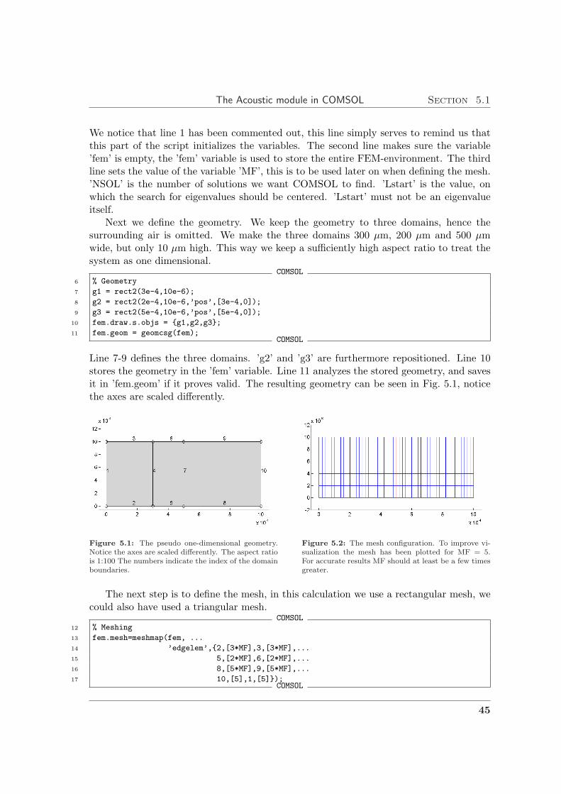
The Acoustic module in COMSOL Section 5.1
We notice that line 1 has been commented out, this line simply serves to remind us thatthis part of the script initializes the variables. The second line makes sure the variable’fem’ is empty, the ’fem’ variable is used to store the entire FEM-environment. The thirdline sets the value of the variable ’MF’, this is to be used later on when defining the mesh.’NSOL’ is the number of solutions we want COMSOL to find. ’Lstart’ is the value, onwhich the search for eigenvalues should be centered. ’Lstart’ must not be an eigenvalueitself.
Next we define the geometry. We keep the geometry to three domains, hence thesurrounding air is omitted. We make the three domains 300 µm, 200 µm and 500 µmwide, but only 10 µm high. This way we keep a sufficiently high aspect ratio to treat thesystem as one dimensional.
COMSOL6 % Geometry
7 g1 = rect2(3e-4,10e-6);
8 g2 = rect2(2e-4,10e-6,’pos’,[3e-4,0]);
9 g3 = rect2(5e-4,10e-6,’pos’,[5e-4,0]);
10 fem.draw.s.objs = g1,g2,g3;
11 fem.geom = geomcsg(fem);COMSOL
Line 7-9 defines the three domains. ’g2’ and ’g3’ are furthermore repositioned. Line 10stores the geometry in the ’fem’ variable. Line 11 analyzes the stored geometry, and savesit in ’fem.geom’ if it proves valid. The resulting geometry can be seen in Fig. 5.1, noticethe axes are scaled differently.
Figure 5.1: The pseudo one-dimensional geometry.Notice the axes are scaled differently. The aspect ratiois 1:100 The numbers indicate the index of the domainboundaries.
Figure 5.2: The mesh configuration. To improve vi-sualization the mesh has been plotted for MF = 5.For accurate results MF should at least be a few timesgreater.
The next step is to define the mesh, in this calculation we use a rectangular mesh, wecould also have used a triangular mesh.
COMSOL12 % Meshing
13 fem.mesh=meshmap(fem, ...
14 ’edgelem’,2,[3*MF],3,[3*MF],...
15 5,[2*MF],6,[2*MF],...
16 8,[5*MF],9,[5*MF],...
17 10,[5],1,[5]);COMSOL
45

Chapter 5 Numerical simulations in COMSOL
Actually this box only contains one real line. The three successive dots simply implies thatthe line is continued below. In line 13 and forth we only define the number of elements onthe outer boundaries. It is important that opposite boundaries have the same number ofelements, otherwise the ’meshmap()’ function will not work. The syntax of the ’edgelem’part is ,’edgelem’,index,[number of elements],index,[number of elements].Hence, we set the boundaries with index 2 and 3 to ’3*MF’, and the boundaries withindex 5 and 6 to ’2*MF’ and so on. In Fig. 5.2 the mesh is plotted for MF=5.
After defining the mesh, the physics are added.COMSOL
18 % Physics
19 fem.appl.mode.class = ’Acoustics’;
20 fem.appl.prop.analysis=’eigen’;
21 fem.appl.equ.cs = 8490,1483,5640;
22 fem.appl.equ.rho = 2331,998.2,2230;
23 fem.appl.equ.ind = [1,2,3];
24 fem.appl.bnd.type = ’SS’,’SH’,’cont’;
25 fem.appl.bnd.ind = [2,2,2,3,2,2,3,2,2,1];COMSOL
When adding the physics we need the governing equations and the boundary conditions.In line 19 the acoustics module is loaded, this module contains the necessary equations,we only have to specify them. This is done in line 20 where the type of analysis is chosento be an eigenfrequency analysis. Hence, the governing equation in all domains becomes,
−1ρ∇2p1+
λe
ρc2s
p1 = 0 (5.9)
Which, fortunately is the exact same as Eq. (5.6) derived above. In line 21 and 22 wedefine the material parameters for three different domain groups, which are distributed tothe three available domains in line 23.
Material Silicon Water PyrexGroup nr. 1 2 3
cs 8490 1483 5640ρ 2331 998.2 2230
Table 5.1: The material parameters for the three different domain groups.
Hence, the leftmost domain receives the parameters of Silicon, the middle domainbecomes water, and the rightmost domain becomes pyrex. We follow the same procedurewhen assigning boundary conditions. First, in line 24 we define three boundary groups.Then in line 25 the groups are distributed. When doing eigenfrequency analysis, threedifferent boundary conditions are available, the soft, the hard and the continuity condition.The soft condition imitates a soft wall, where the particles are free to oscillate back andforth. Hence, the soft boundary condition is defined as,
p1 = 0. (5.10)
To see how this relates to the particle velocity, we recall from Eq. (3.24) that for a timeharmonic pressure we have ϕ1 = −ip1/ρ0ω. Hence, u1 = ∇ϕ1 = −i∇p1/ρ0ω. The soft
46

The Acoustic module in COMSOL Section 5.1
condition therefore gives no constraints on u1. The hard condition imitates a hard wall,where the particle velocity is fixed to the steady wall. The hard boundary condition isdefined as,
n·∇p1
ρ0
= 0. (5.11)
This condition locks the particle velocity, but leaves no constraint on the pressure. Thecontinuity condition simply states that both pressure and particle velocity must be con-tinues across the boundary. The continuity condition can only be applied to internalboundaries. The question, that now remains, is how to distribute these three conditionto the ten boundaries in our problem. First we notice that boundary 4 and 7 are internalboundaries. Hence, it is obvious that these should be of the continues type. Since we wantto compare this system with one placed on top of a piezo element. The boundary facingthe piezo is forced to move together with the piezo, hence boundary 1 should be of typehard. Since boundary 10 is supposed to be adjacent to normal air it should be free tomove, and hence, be of the type soft. The remaining boundaries are all set to be of thehard type, as this makes the pressure constant across the boundaries. This mean that thesystem will act as one dimensional, as long as the shortest wavelength is more than twiceof the height of the domains. The speed of sound is lower in water than in silicon andpyrex, so the smallest wavelengths will be in the water domain. We can therefore find thecritical frequency as,
Fc =cs
2λ≈ 1500 ms−1
20× 10−6 m≈ 75 MHz. (5.12)
This result is very important, as it tells us that all eigenfrequencies found to be more than75 MHz are not valid. Line 25 distributes the boundary groups in the following way:
Boundary type Hard (SH) Soft (SS) Continues (cont)Boundary number 1, 2, 3, 5, 6, 8, 9 10 4, 7
Table 5.2: The distribution of the boundary conditions. The letters in the parenthesis are the abbreviations usedin line 24.
Now the problem has been fully defined we begin to solve it. Before the actual solving stepthe FEM-structure must be prepared. This is done in line 27-28, where we use the functions’multiphysics()’ and ’meshextend()’, which combines the defined physics applications withthe defined mesh.
COMSOL26 % Solving
27 fem=multiphysics(fem);
28 fem.xmesh=meshextend(fem);
29 fem.sol=femeig(fem, ...
30 ’neigs’,NSOL, ...
31 ’shift’,Lstart, ...
32 ’solcomp’,’p’, ...
33 ’outcomp’,’p’);COMSOL
47

Chapter 5 Numerical simulations in COMSOL
In line 29 the eigensolver, femeig() is called. We use the argument ’neigs’ to tell thesolver how many solutions we are looking for. In this case we are looking for NSOL, whichwas set to four in line 4. The next argument is ’shift’, which tells the solver where to beginthe search for solution. Since we in this example wants the first four eigenvalues we set’shift’ to Lstart, which was set to 500 in line 5. Finally we tell the solver to solve for thespecific variable , p, representing pressure. Finally we take a look at the results.
COMSOL34 % Plotting
35 for j=1:length(fem.sol.lambda)
36 figure
37 postcrossplot(fem,1,[0 0.001;5e-6 5e-6], ...
38 ’lindata’,’p’, ...
39 ’solnum’,j);
40 end
41 (fem.sol.lambda.^0.5./(2*pi))’COMSOL
The lines 35 and 40 starts and ends a loop, which is executed once for each found solution.The variable ’j’ serves as a counter, hence, it refers to the current solution number. Line36 creates a new figure window, to avoid the coming plots from overlapping each other. Inline 37-39 we make a cross section plot of the pressure. The argument in square brackets iscoordinates for the cross section. Since the simulation is supposed to be one dimensionalthe y-coordinates are unimportant as long as they are identical. The x-coordinates are 0and 0.001. In line 38 we tell the plotter that it is the pressure we wish to see plotted. Line39 makes sure we plot the j’th solution. Finally in line 41 we ask the script to computeand print the found eigenfrequencies. In Fig. 5.3 the output from the script is shown,however only the third solution-plot is shown.
Resultans =
1.0e+006 *
0.4746
3.5581
5.5887
6.7202Result
Figure 5.3: The left side of this figure shows the output of the script, while the right side shows a cross sectionplot of the pressure distribution corresponding to the third eigenfrequency. The four found eigenfrequencies are 0.47MHz, 3.56 MHz, 5.59 MHz and 6.72 MHz.
When using the eigenfrequency analysis we must be aware that there might be solu-tions, which has not been found, and a second execution of the script may yield a differentresult. This problem seems only to apply to the ends of the eigenvalue list. So for anyother purposes than this example the number of eigenvalues sought should be large enoughto allow the exclusion of a few values at each end of the list. If the list starts at zero, asin this example, the first eigenvalues should all be found. Notice that the second eigen-
48
The Acoustic module in COMSOL Section 5.1
frequency corresponds to the one shown in Fig. 4.3 panel (c), while we will look at thethird resonance in the next subsection.
5.1.3 The time harmonic solver
To see how the pressure will distribute in our sandwich structure for any given frequency,we must make a time harmonic analysis. For this analysis we add a new domain to the rightside of the geometry from the eigenfrequency analysis. This domain represent the ambientair. The governing equations for time harmonic analysis is the same, however a few moreboundary conditions are added. When loading the acoustic module, COMSOL will selectthe harmonic analysis by default, hence, the line fem.appl.prop.analysis=’eigen’;must be omitted. In this analysis we include two new boundary conditions, one to describehow the piezo element(not included in model) effects the adjacent boundary, and one todescribe how the sound waves leak to the surroundings. To model a vibrating piezo elementwe use the normal acceleration boundary condition.
n·∇p1
ρ0
= an. (5.13)
Fortunately, we have already determined the inward acceleration, an. From Eq. (4.2)we have aw = −i`ω2ne−iωt, where ` is the amplitude of the piezo, and ω is the angularfrequency. When choosing ω we must be sure to stay below the critical frequency, since ourmodel still is pseudo-one-dimensional. To implement the normal acceleration boundarycondition the type abbreviation ’NA’ is used. The acceleration is introduced with the linebnd.nacc = a;. To model the leakage of sound waves, we use the impedance boundarycondition
n·∇p1
ρ0
− iωp1
Z= 0. (5.14)
The origin of this equation is the same assumption as we used in Section 4.3, which wasthat there should be no reflected wave, Dl = 0. This can be seen by remembering thatthe wave, in domain D has the form p1,D(x, t) = Dre
i(kDx−ωt) + Dlei(−kDx−ωt). We then
perform the following manipulation,
n·∇p1
ρ0
− iωp1
Z= 0, (5.15)
∂x
(Dre
i(kDx−ωt)
ρ0
+Dle
i(−kDx−ωt)
ρ0
)− iωDre
i(kDx−ωt)
Z− iωDle
i(−kDx−ωt)
Z= 0, (5.16)
ikDDrei(kDx−ωt)
ρ0
− ikDDlei(−kDx−ωt)
ρ0
− iωDrei(kDx−ωt)
Z− iωDle
i(−kDx−ωt)
Z= 0. (5.17)
We then use k = w/c and Z = ρ0c
iωDrei(kDx−ωt)
Z− iωDle
i(−kDx−ωt)
Z− iωDre
i(kDx−ωt)
Z− iωDle
i(−kDx−ωt)
Z= 0, (5.18)
−2iωDle
i(−kDx−ωt)
Z= 0, (5.19)
49
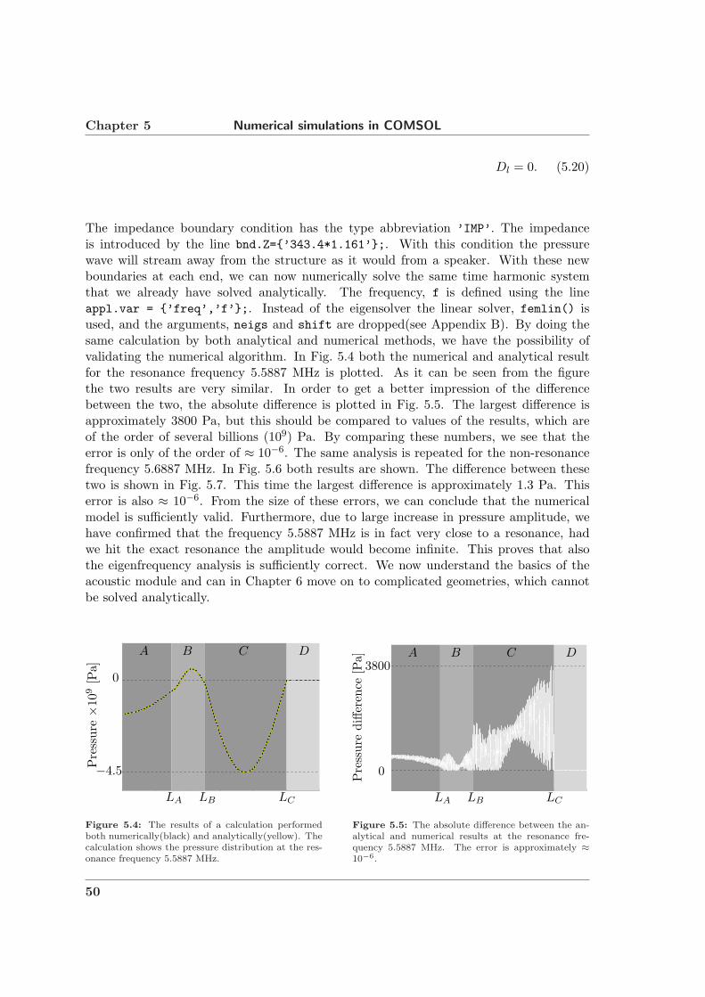
Chapter 5 Numerical simulations in COMSOL
Dl = 0. (5.20)
The impedance boundary condition has the type abbreviation ’IMP’. The impedanceis introduced by the line bnd.Z=’343.4*1.161’;. With this condition the pressurewave will stream away from the structure as it would from a speaker. With these newboundaries at each end, we can now numerically solve the same time harmonic systemthat we already have solved analytically. The frequency, f is defined using the lineappl.var = ’freq’,’f’;. Instead of the eigensolver the linear solver, femlin() isused, and the arguments, neigs and shift are dropped(see Appendix B). By doing thesame calculation by both analytical and numerical methods, we have the possibility ofvalidating the numerical algorithm. In Fig. 5.4 both the numerical and analytical resultfor the resonance frequency 5.5887 MHz is plotted. As it can be seen from the figurethe two results are very similar. In order to get a better impression of the differencebetween the two, the absolute difference is plotted in Fig. 5.5. The largest difference isapproximately 3800 Pa, but this should be compared to values of the results, which areof the order of several billions (109) Pa. By comparing these numbers, we see that theerror is only of the order of ≈ 10−6. The same analysis is repeated for the non-resonancefrequency 5.6887 MHz. In Fig. 5.6 both results are shown. The difference between thesetwo is shown in Fig. 5.7. This time the largest difference is approximately 1.3 Pa. Thiserror is also ≈ 10−6. From the size of these errors, we can conclude that the numericalmodel is sufficiently valid. Furthermore, due to large increase in pressure amplitude, wehave confirmed that the frequency 5.5887 MHz is in fact very close to a resonance, hadwe hit the exact resonance the amplitude would become infinite. This proves that alsothe eigenfrequency analysis is sufficiently correct. We now understand the basics of theacoustic module and can in Chapter 6 move on to complicated geometries, which cannotbe solved analytically.
A B C D
LA LB LC
0
−4.5
Pre
ssure
×10
9[P
a]
Figure 5.4: The results of a calculation performedboth numerically(black) and analytically(yellow). Thecalculation shows the pressure distribution at the res-onance frequency 5.5887 MHz.
A B C D
LA LB LC
0
3800
Pre
ssure
diff
eren
ce[P
a]
Figure 5.5: The absolute difference between the an-alytical and numerical results at the resonance fre-quency 5.5887 MHz. The error is approximately ≈10−6.
50

General PDE formulation for COMSOL Section 5.2
A B C D
LA LB LC
0
−1.5
Pre
ssure
×10
6[P
a]
Figure 5.6: The results of a calculation performedboth numerically(black) and analytically(yellow). Thecalculation shows the pressure distribution at the non-resonance frequency 5.6887 MHz.
A B C D
LA LB LC
0
1.3
pre
ssure
diff
eren
ce[P
a]
Figure 5.7: The absolute difference between the an-alytical and numerical results at the non-resonancefrequency 5.6887 MHz. The error is approximately≈ 10−6.
5.2 General PDE formulation for COMSOL
In Chapter 3 we derived three equations necessary for finding u′′2. The three partialdifferential equations we wish to solve using COMSOL, are the compressible continuityequation Eq. (3.61)
∂xu′′2 + ∂yv′′2 = S (5.21)
and the x and y components of the steady-state Navier-Stokes equation Eq. (3.62)
η∇2u′′2 =∂xp′′2 + F ′′x − βη∂x
(∂xu′′2 + ∂yv
′′2
)(5.22)
η∇2v′′2 =∂yp′′2 + F ′′
y − βη∂y
(∂xu′′2 + ∂yv
′′2
)(5.23)
where S, F ′′x and F ′′
y are known functions of both x and y. These three equation each hasan associated dependent variable. The continuity equation has p′′2 (∂tp
′′2 + ∇·J ′′2 = 0), and
the x and y component of the Navier-Stokes equation has u′′2 and v′′2 , respectively. Hence,we have the three dependent variables a = u′′2, v′′2 or p′′2. Each of the three equationsEqs. (5.21 - 5.23) must be formulated using the general PDE formulation,
∇·Γa = fa. (5.24)
where all terms containing the associated dependent variable, a, are collected in the vectorΓa. All other terms are listed in the scalar fa
Γp′′2 =(
00
), fp′′2 = −(∂xu′′2 + ∂yv
′′2) + S (5.25)
Γu′′2 =(
(β + 1)η∂xu′′2η(∂yu
′′2 + β∂xv′′2)
), fu′′2 = ∂xp′′2 + F ′′
x (5.26)
51

Chapter 5 Numerical simulations in COMSOL
Γv′′2 =(
η(∂xv′′2 + β∂yu′′2)
(β + 1)η∂yv′′2
), fv′′2 = ∂yp
′′2 + F ′′
y (5.27)
In the general PDE formulation, the boundary conditions are defined as a combination ofa Dirichlet and a Neumann condition
−n·Γa = Ga + µ(∂aRa
)T; Ra = 0, (5.28)
where a is the dependent variable associated to Γa, µ is the Lagrange multiplier and Ga
and Ra are to be specified. n is normal vector of the boundary. If we define Ra ≡ 0, thenthe term ∂aRa becomes zero, and since the Dirichlet condition (0 = 0) does not contributewith any restraints, the only remaining condition is the Neumann condition
−n·Γa = Ga. (5.29)
If we instead define Ra, for instance Ra ≡ a − 4, so the term ∂aRa differs from zero,then the Lagrange multiplier can be scaled to achieve any desired value. Hence the entireNeumann condition can be discarded and any definition of Ga becomes obsolete. The onlyremaining condition is the Dirichlet condition a− 4 = 0 or
a = 4. (5.30)
If we define Ra 6= 0 such that ∂aRa = 0 we get both Dirichlet and the Neumann condition.For internal boundaries the definition is slightly different
−n·(Γa,1 − Γa,2) = Ga + µ(∂aRa
)T; Ra = 0; a1 = a2, (5.31)
where the numeric subscripts refer to the two adjacent domains divided by the boundary.We notice that this condition requires the dependent variable to be continues across theboundary (see Appendix D).
5.3 Executing a COMSOL-script
To execute a COMSOL-script, both Matlab and COMSOL must be installed. The pro-grams are simultaneously initiated by the command
C:\COMSOL32\bin\comsol.exe matlab.
This command will most likely already exist as a shortcut in the ’programs’-folder. Whenthe programs are up and running, the script can be entered into the Matlab-editor. Oncethe script has been entered, it can be executed by hitting the ”F5”-button. A selectedpart of the script can be executed by the ”F9”-button.
52

Chapter 6
The acoustic radiation force
6.1 The force in one dimension
When a microfluidic channel is affected by a standing acoustic wave, any suspended parti-cles will be affected by a force called the ’acoustic radiation force’, Far. The induced forcewill move particles towards either pressure nodes or anti-nodes. The acoustic radiationforce is commonly [16] quoted in one dimension as
Far =−(
πp21Vp
2λ
)φ(β, ρ) sin(2kd) (6.1)
whereφ(β, ρ) = βl
5ρp−2ρl
2ρp+ρl−βp (6.2)
and
p1 = Pressure amplitude.Vp = Volume of the particle.d = Distance from closest pressure node(p1).λ = Wavelength of the acoustic wave.k = 2π
λβl, βp = Compressibility of either the liquid or the particle.ρl, ρp = Density of either the liquid or the particle.
By looking at Eq. (6.1) it is clear that once the standing wave is achieved, severaldifferent factors has influence on the size of the force. First of all the pressure amplitude,this can somewhat be controlled by the tone generator connected to the piezo element andby ensuring that the element is properly connected to the chip, but it is mainly a matterof how perfect a resonance is achieved. The second factor is the volume of the particles, itsimply implies that the larger a particle; the greater the force(more on this in Chapter 8).Note that the particles must be smaller than half of the wavelength. The third factor isthe wavelength, since the force decreases as wavelength increases, higher frequencies yieldshigher force. The fourth factor is φ(β, ρ), this factor is determined by the characteristics
53
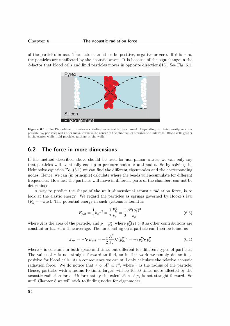
Chapter 6 The acoustic radiation force
of the particles in use. The factor can either be positive, negative or zero. If φ is zero,the particles are unaffected by the acoustic waves. It is because of the sign-change in theφ-factor that blood cells and lipid particles moves in opposite directions[18]. See Fig. 6.1.
Figure 6.1: The Piezoelement creates a standing wave inside the channel. Depending on their density or com-pressibility, particles will either move towards the center of the channel, or towards the sidewalls. Blood cells gatherin the center while lipid particles gathers at the walls.
6.2 The force in more dimensions
If the method described above should be used for non-planar waves, we can only saythat particles will eventually end up in pressure nodes or anti-nodes. So by solving theHelmholtz equation Eq. (5.1) we can find the different eigenmodes and the correspondingnodes. Hence, we can (in principle) calculate where the beads will accumulate for differentfrequencies. How fast the particles will move in different parts of the chamber, can not bedetermined.
A way to predict the shape of the multi-dimensional acoustic radiation force, is tolook at the elastic energy. We regard the particles as springs governed by Hooke’s law(Fh = −ksx). The potential energy in such systems is found as
Epot =12ksx
2 =12
F 2h
ks=
12
A2(p′′2)2
ks(6.3)
where A is the area of the particle, and p = p′′2, where p′′2(r) > 0 as other contributions areconstant or has zero time average. The force acting on a particle can then be found as
Far = −∇Epot = −12
A2
ks∇(p′′2)
2 = −τp′′2∇p′′2 (6.4)
where τ is constant in both space and time, but different for different types of particles.The value of τ is not straight forward to find, so in this work we simply define it aspositive for blood cells. As a consequence we can still only calculate the relative acousticradiation force. We do notice that τ ∝ A2 ∝ r4, where r is the radius of the particle.Hence, particles with a radius 10 times larger, will be 10000 times more affected by theacoustic radiation force. Unfortunately the calculation of p′′2 is not straight forward. Sountil Chapter 8 we will stick to finding nodes for eigenmodes.
54

Dimensional analysis; from 3D to 2D Section 6.3
6.3 Dimensional analysis; from 3D to 2D
The obvious way to calculate the resonance pressure field, is a three dimensional eigenfre-quency analysis. When trying to model the chip presented in Section 1.3.1 in three dimen-sions, it proved to be a complicated matter to define the mesh. Usually a mesh of isotropictetrahedron is used. However, this is not a possibility because of the Length:width:heightratio being 47:15:1, meaning that if we wish to have 15 elements in the height, which still isa rather low resolution, we would end up with approximately (15×1)×(15×15)×(15×47) ≈2.4 × 10⁶ elements. With so many elements the calculation would require far more phys-ical memory than is found in a standard computer. So, in order to obtain anisotropicelements we must use an extruded mesh of quadrilaterals. The extrusion, however, forcesus to model each layer independently, in order to define several different domains in thez-direction. The three layers are then connected using ’Identity Boundary Conditions’.However, it quickly proved that also this combination of still many elements and the iden-tity boundary conditions, also required far too much computational power. This meantthat it would be necessary to figure out if the calculations could be made in only twodimensions.
6.3.1 Validation of the 2D approximation
Instead of doing the calculation i three dimension it is suggested, that due to the rela-tive low frequency(or long wavelengths) we can neglect the z-direction, and perform thecalculation on a two dimensional cross section of the second layer. In order to validatethe results of a two dimensional approximation, a new geometry was invented(only forsimulation purposes). The plan was to simplify the geometry so much that it would bepossible to perform full three dimensional simulations. The results of the two- and threedimensional simulations could then be compared. The new geometry took root in the oldone. The chamber was kept at 2mm×2mm while the channel was shorted down, so it onlyextended 2.4 mm on each side of the channel. The distance from the end of the channel tothe edge of the chip was shortened to 0.6 mm, giving the new chip a total length of only8 mm. The distance from the chamber to the edge of the chip was shortened to 2 mm oneach side. Hence, resulting in a total width of 6 mm. The Heights of the three layers werekept at original values. By cutting down the chip size three dimensional eigenfrequencyanalysis became possible, but only for a very coarse mesh. When doing finite element sim-ulations it is very important to keep the wavelengths larger than the mesh size, otherwisethe problem cannot be well defined. Hence, in order to keep the wavelengths long enough,we only calculate the first 49 eigenfrequencies. The new smaller geometry is convertedinto two dimensions and solved using the same coarse mesh. Since we do not expect thesolutions to be in the exact same order in two and three dimensions, we calculate the first50-two dimensional eigenfrequencies. To compare the calculated pressure fields, a crosssection in the xy-plane in the middle of the chamber were visually compared. Only the50th two-dimensional solution could not be matched. Had the three dimensional analysisreached further a matching solution might have been found. Hence, the 50th solution isdiscarded. In Fig. 6.2 the results from the three dimensional calculation have been plot-
55

Chapter 6 The acoustic radiation force
ted(with a blue ’x’). In the same figure the results from the two dimensional calculation,which had a similar pressure field to one of the three dimensional solutions, have also beenplotted(with a red ’o’). In Fig. 6.3 the solutions are sorted based on the two dimensionalsolutions. From the lack of gaps in these two figures we can conclude that for low fre-quencies, the same pressure fields exist for both the two and three dimensional geometries.Furthermore, the shift between two frequencies, corresponding to the same pressure field,is almost constant at 0.5 MHz.
3D
2D
0 10 20 30 40 500
0.5
1
1.5
2
2.5
3
Fre
quen
cy[M
Hz]
Solution No.
Figure 6.2: Both 2D and 3D solutions sorted basedon the three-dimensional solutions. The lack of gaps inthe two-dimensional solutions indicate that all calcu-lated three-dimensional pressure fields were also foundin the two dimensional calculation.
3D
2D
0 10 20 30 40 500
0.5
1
1.5
2
2.5
3
Fre
quen
cy[M
Hz]
Solution No.
Figure 6.3: The figure show both 2D and 3D solutionssorted based on the two dimensional solutions. Thelack of gaps in the three dimensional solutions indicatethat all calculated two dimensional pressure fields werealso found in the three dimensional calculation.
This shows us that even though there is a shift in frequency, all pressure fields can befound from the two dimensional analysis as long as the frequency is low enough to preventwaves in the z-direction.
6.3.2 Density of states
The curves in Figs. 6.2 and 6.3 can be approximated analytically by assuming we onlyhave one domain, where the speed of sound is an average value of those otherwise present.From the analytical solution (Eq. (5.7)) we have the relation
ω2 = c2sπ
2
(n2
a2+
m2
b2+
l2
c2
). (6.5)
From this equation we calculate the frequency for any integer combination of n,m andl. The results are sorted in increasing order and plotted in Fig. 6.5 as ’analytical fit’.Furthermore we can approximate this by rewriting Eq. (6.5) as
ω2
c2s
= k2, (6.6)
where k is defined ask = (kx, ky, kz) =
(πn
a,πm
b,πl
c
). (6.7)
56

Dimensional analysis; from 3D to 2D Section 6.3
Hence,ω
cs= |k|. (6.8)
To find the number of solutions below a given frequency, we divide the area/volume of thecircle/sphere with radius |k|, by the area/volume of a single solution. In Fig. 6.4 the twodimensional analogy is shown.
|k| = 2
1 2
2
1
kx
ky
k=
(kx, ky
)
Figure 6.4: The definition of k, which can be used to determine the density of states. For enhanced visibility onlythe two dimensional case is shown.
Hence, we find the number of solutions to be
N3D(f) =Vsphere
Vsol=
43π|k|3πa
πb
πc
=4 (2πf)3 a b c
3 c3s π2
. (6.9)
By turning this equation around we can predict the frequency of the N’th solution,
f3D(N) =cs
2π
3
√3π2
43
√N
abc. (6.10)
The same procedure is valid for two dimensional problem.
N2D(f) =Acircle
Asol=
π|k|2πa
πb
=(2πf)2 a b
c2s π
. (6.11)
f2D(N) =cs
2π
√Nπ
ab(6.12)
We then plot the frequency as a function of the solution number, for both the two and threedimensional analysis, together with the simulation results. For the analytical solutions thespeed of sound have been fitted to fit the simulations. The reason for this is that theredoes not seem to be an obvious way to estimate the speed of sound. We could have usedthe sum of the speeds in each domain and divide by the number of domains. However,we must also take into account that each speed should be weighted by the relative size of
57

Chapter 6 The acoustic radiation force
the corresponding domain. Furthermore, domains with a low speed of sound, will supportmore solutions, and should somehow be emphasized. From Fig. 6.5 it is seen that theshape of the analytical approximations are relatively close to the simulation results. Thisindicate the applied eigenfrequency solver have not skipped any solutions, nor has it foundartificial solutions originating from bad meshing amongst other modeling features.
0
0.5
1
1.5
2
2.5
3x 10Analytic approximation(2D)Analytic approximation(3D)Analytic fit2D3D
0 10 20 30 40 500
0.5
1
1.5
2
2.5
3
Fre
quen
cy[M
Hz]
:o) Solution No.
Figure 6.5: Comparison of the analytical eigenfrequencies to those from the simulations. For the 3D and 2Dapproximations and the analytical fit we used c3D = 8400m/s, c2D = 7500m/s and cFit = 5250m/s
We have now shown that as long as we stick to low frequencies all pressure fields can befound using only a two dimensional analysis. Furthermore, the f(N)-curves follow thoseanalytically predicted. Hence, we can generalize these conclusions to also apply for theoriginal geometry shown in Fig. 1.1. Should this generalization be valid, we are now ableto simulate the pressure fields inside the real chip.
6.4 The symmetric chamber model
In Section 6.3 we have shown that it is sufficient to perform the simulations in only twodimensions. However, the two original chips used in the experiments, were designed foreasy fabrication and handling. At that time it was not considered to design the chips witha geometry, which could easily be remodeled. This meant that parts of the chips easilybroke off leaving unpredictable shapes. Hence, the simulated geometries should not beconsidered exact replicas, but rather geometric approximations. Since the geometry willnot be exact anyway, we look at the simplest working approximation. The large differencein the acoustic impedance between silicon and water,
Zw
Zsi
=cwρw
csiρw=
1483 m s−1 × 998.2 kg m−3
8490 m s−1 × 2331 kg m−3= 0, 075 (6.13)
allows us to treat the water/silicon interface as a hard wall. Hence, we can discard thesilicon domain and only simulate the domains containing liquid. Hence, we rather discardthe silicon domain that simulate it using wrong dimensions. By this approximation thegeometry simplifies to a 2 mm× 2 mm chamber, centered on a 25 mm× 0.4 mm channel
58

The symmetric chamber model Section 6.4
(see Fig. 6.6). The boundary conditions are set to hard wall, n ·∇p1 = 0, except at thetwo ends of the channel were we set p1 = 0 to mimic the in- and outlets. This geometrywill here forth be called the symmetric chamber model.
2 mm
25 mm
2 mm0.4 mm
Figure 6.6: The chamber model
The system could of cause be approximated even further, by simply simulating thechamber itself, but this have proved to be too rough an approximation, as the foundeigenmodes could not be experimentally confirmed.
The result of the simulations(see Appendix C) on both the square and the circularsymmetric chamber model yielded several hundreds of eigenmodes in the frequency range0.5 MHz − 3 MHz, from which only a small fraction could be experimentally verified. Itis difficult to predict which of the calculated eigen-modes will be possible to determineexperimentally, as the pressure field amplitude is normalized to fulfill
∫Ω p2
1 dxdy∫Ω 1 dxdy
= 1. (6.14)
However, if the calculation shows a much higher amplitude in the chamber than in thechannel, the probability of experimentally observing this mode is greatly increased. Someof the results are shown in Fig. 6.7. Notice that the shown examples have been chosenbased on their geometric differences, and not based on the quality of the frequency match.
59

Chapter 6 The acoustic radiation force
(1a) 0.73 MHz (1b) 0.67 MHz (2a) 2.49 MHz (2b) 2.42 MHZ
(3a) 1.35 MHz (3b) 1.28 MHz (4a) 2.23 MHz (4b) 2.17 MHz
Figure 6.7: Four examples of how the simulated eigenmodes can be confirmed by experiments. The top row isfrom a chip with a round chamber, while the bottom row is a square chamber. We see that the simulated frequenciesdoes not match the experimental ones completely. Panel (2b) courtesy Melker Sundin.
Fig. 6.7 compares the simulated eigenmodes with the experimental obtained beadpatterns. An important lesson learned from studying these pictures, is that the beads notonly accumulate at the nodal-lines, but seems to be more confined to the nodal-line thesteeper the gradient of eigenmode pressure field is at that location. This is especially clearin panel (1b) and (2b) but can also be seen in panel (3b) This strongly indicates that thedefinition of the acoustic radiation force, Far, should include a term dependant on thespatial derivative of p. We notice this is not the case in Eq. (6.1) but in Eq. (6.4). Whenlooking at panel (4b) we see that some beads have accumulated at the pressure extremes.These are in fact a different kind of beads than the blood cell phantoms, and apparentlythese other beads have an opposite compressibility ratio than blood cells. (τ < 0 inEq. (6.4)). An important feature not revealed by Fig. 6.7 is the strength of the acousticradiation force. In panel (1b) and (3b) the force was extremely weak, while a little strongerin panel (2b). In the final case of panel (4b) the force was many times stronger than inother eigenmodes. The pattern formed at 2.17 MHz was the only observed pattern strongenough to withstand a flow through the chamber. All other patterns were immediatelywashed away. We notice that there seems to be a small offset between the calculatedfrequencies and the corresponding experimental ones. This offset might be caused byvariations in the temperature during the experiments. Despite the small deviation infrequency the simulations are very precise for describing where the beads will accumulate.
6.5 Breaking of symmetry
Since the original chips were asymmetric, some of the experimentally observed eigenmodesalso were. These eigenmodes can not be explained from the symmetric chamber model,
60

Breaking of symmetry Section 6.5
so to ensure our understanding we must expand the model. In reality the chambers wereplaced off center relative to the channel on both chips. Furthermore the channel/chamberregion was shifted in both x- and y-direction, also on both chips. All these shifts could ofcause be implemented at once, but it proved very difficult to estimate the correct lengthsof these shifts. This meant that only some of the experimentally observed eigenmodescould be found for a set of shift-length-parameters. So instead of wasting time searchingfor the exact values of the parameters, it was decided to just break the symmetry in asimple way. There are two obvious ways to bring asymmetry into the system (see Fig. 6.8).
(a) (b)
Figure 6.8: Two simple ways of introducing asymmetry to the model. In panel (a) the chamber/channel parthas been shifted as a whole. This method requires that the surrounding silicon is also simulated. In panel (b) thechamber has been shifted relative to the channel. The dotted line indicate former symmetry lines.
One way is to simulate the surrounding silicon in which both the channel and chamberboth has been shifted slightly, or a second and easier way is to shift the location of thechamber relative to the channel. In Fig. 6.9 we compare the experimental patterns withthose achieved using the two asymmetric models. Panel (a) and (b) shows the asymmetricpatterns corresponding to 2.06 MHz and 2.08 MHz, respectively. We notice how the leftside appear strongest in panel (a) and the right one in panel (b). Panel (c) and (d)shows the corresponding results from simulations on the asymmetric model where siliconsurrounds the liquid region. The liquid region is shifted 0.5 mm right and 0.5 mm up. Thedifference in frequency between panel (c) and (d) is only 1 kHz. When we compare panel(c) and (d) to panel (a) and (b), we notice how the blue(low) areas just left and right ofthe red(high) center peak is of different strengths. In panel (c), as well as in panel (a) wesee that left side is the strongest. In panel (d) and (b) it is the other way around. Hence,the method of applying an asymmetric silicon part around the chamber is sufficient toaccount for the split eigenmode.
61

Chapter 6 The acoustic radiation force
(a) (b)
(c) (d)
(e) (f) (g)
Figure 6.9: Panel (a) and (b) shows the asymmetric patterns corresponding to 2.06 MHz and 2.08 MHz, respec-tively. Panel (c) and (d) shows the corresponding results from simulations on the asymmetric model where siliconsurrounds the liquid region. The liquid region is shifted 0.5 mm right and 0.5 mm up. The difference in frequencybetween panel (c) and (d) is only 1 kHz. Panel (e) and (g) shows the result of shifting the otherwise symmetricplaced chamber 1 mm to the right. The frequency difference is 28 kHz. Panel (f) shows the corresponding symmetricsolution. Panel (a) and (b) courtesy Melker Sundin.
Panel (e) and (g) shows the result of shifting the, otherwise symmetric placed, chamber1 mm to the right relative to the channel. The frequency difference between panel (e) and(g) is 28 kHz. Panel (f) shows the corresponding symmetric eigenmode solution. Bycomparing the nodal lines(black) in panel (e) and (g) to the experimental bead patterns,we can see that this very simple approach also can explain the eigenmode splitting.
62
Concluding remarks Section 6.6
6.6 Concluding remarks
We have shown that for a relatively shallow chamber, it is sufficient to find the eigenmodesfor the governing Helmholtz equation in two dimensions instead of three, as long as thewavelength is more than twice the length of the third dimension. One consequence ofusing the Helmholtz equation for unattenuated waves is that simulations yields far moresolutions than can be experimentally verified. This can be explained by arguing that, inthe laboratory, acoustic damping in the liquid and any energy dissipation will smear outthe theoretically perfect peaks. Hence, some modes will entirely disappear, while othersmight be clouded by stronger modes. The mismatch in frequency between experimentaland calculated values, can be related to geometric uncertainties and thermally inducedchanges to material parameters.
Furthermore it has been shown that it is not necessary to include the material sur-rounding the chamber and channel (silicon in this case), as long as there is a large acousticimpedance mismatch.
It has also been shown that if the symmetry is broken the eigenmodes will spilt up.So finally it can be concluded that the chamber model is very effective, when calculating
where beads will accumulate.
63


Chapter 7
Examples of sound absorption in liquids
In this chapter we will look at some examples of how to calculate the second-order termsfrom Section 3.3.3. We start with two one-dimensional systems and finally in Section 7.3we look at a two-dimensional system. In each example we calculate the first-order termsbefore we can find the second-order terms.
7.1 Analytic Example 1: plane traveling wave
In the first example we study a liquid under influence of a plane harmonic traveling wave.The wave is created by a oscillating wall at x = 0. Where the positive half space iscontaining the liquid. This system can be regarded as one dimensional. k0 = ω/c0 and γis the viscous damping parameter.
7.1.1 First order pressure, p1, and velocity u1
Since we prefer to use a steady coordinate system, we model the oscillation of the wall bystating that the flux at x = 0 is oscillating with the angular frequency ω ≈ 106 s−1 andthe amplitude ` ≈ 10−9m.
J1(x, t) = ρ0u1 = ρ0ω`e−iωt. (7.1)
Hence, we may assume the velocity field, u1, and the pressure field p1 has the form
u1(x, t) = ω`eϕ(x,t), (7.2)
and
p1(x, t) =p1
ω`u1(x, t) = p1e
ϕ(x,t), (7.3)
whereϕ(x, t) = (i− γ)k0x− iωt, (7.4)
and
γ =(β + 1)ωη
2ρ0c20
. (7.5)
65

Chapter 7 Examples of sound absorption in liquids
We note that Eq. (7.3) already fulfills the one dimensional edition of Eq. (3.51)
∂2xp1 =− k2
0
[1 + iγ
]2
p1. (7.6)
To find p1(x), we insert u1 and p1 into the one dimensional edition of Eq. (3.47)
∂2xu1 =− i
ωρ0
ηu1 +
[1− i
ωηβ
ρ0c20
]1η∂xp1, (7.7)
we find
p1 =[1 + iγ
]ρ0c0ω`. (7.8)
To summarize the first order terms we got
u1(x, t) = εc0eϕ(x,t), (7.9)
p1(x, t) = p1eϕ(x,t) = ε(1 + iγ)ρ0c
20e
ϕ(x,t), (7.10)
where we have introduced the perturbation parameter ε
ε =ω`
c0
≈ 10−6. (7.11)
We can now calculate the second order terms.
7.1.2 Second order pressure, p′′2, and velocity u′′2
We can now begin to solve the one dimensional editions of Eq. (3.61) and Eq. (3.62)
∂xu′′2 = − 12c2
0ρ0
∂xRe[p1u
∗1
], (7.12)
η∂2xu′′2 + βη∂x(∂xu′′2) =∂xp′′2 + F ′′
(β + 1)η∂2xu′′2 =∂xp′′2 + F ′′ (7.13)
We insert the known first order terms into Eq. (7.12) and integrate to find u′′2
u′′2 =− 12c2
0ρ0
∫ (∂xRe
[p1u
∗1
])dx
=− 12c2
0ρ0
Re[p1u
∗1
]+ Cu
=− 12c2
0ρ0
c30ε
2ρ0e−2k0γx + Cu
=− ε212c0e
−2k0γx + Cu. (7.14)
66

Analytic Example 1: plane traveling wave Section 7.1
where Cu is an integration constant. Next we calculate F ′′ according to Eq. (3.38) in onedimension
F ′′ =12ρ0Re
[u1∂xu∗1
]+
12ρ0Re
[u1∂xu∗1
]
= ρ0Re[u1∂xu∗1
]
= −ε2γc0ωρ0e−2k0γx. (7.15)
We can now find p′′2 by inserting Eq. (7.14) and Eq. (7.15) into Eq. (7.13) and integrate
∂xp′′2 =(β + 1)η∂2xu′′2 − F ′′
p′′2 =∫ [
(β + 1)η∂2xu′′2 − F ′′
]dx
p′′2 =ε2γc0ωρ0
∫ [(1− 4γ2)e−2k0γx
]dx
p′′2 =− ε212c20ρ0(1− 4γ2)e−2k0γx + Cp (7.16)
where Cp is an integration constant. Here we assume Cp ≡ 0.We now calculate the time averaged flux J ′′2 . Keeping in mind that in a one dimensional
system with one wall the time-averaged flux must be zero in steady state, otherwise someareas of the system would end up depleted.
J ′′2 = 〈ρ1u1〉t + ρ0u′′2 = 0. (7.17)
We can quickly see that
ρ0u′′2 =− ε2
12c0ρ0e
−2k0γx + ρ0Cu. (7.18)
and that
〈ρ1u1〉t =12Re
[p1
c20
u∗1
]
=ε212c0ρ0e
−2k0γx. (7.19)
Hence, we find
J ′′2 = −ε212c0ρ0e
−2k0γx + ε212c0ρ0e
−2k0γx + ρ0Cu = 0, (7.20)
if Cu = 0. From Eq. (6.4) we have the acoustic radiation force
Far =− τp′′2∂xp′′2
=ε4γ
2τρ2
0c30(1− 4γ2)e−4k0γx (7.21)
we notice that for all positive x values, the radiation force is also positive. Hence, theparticles are repelled by the oscillating wall.
67


Analytic Example 2: Wave resonance, 1D Section 7.2
7.2 Analytic Example 2: Wave resonance, 1D
The second example concerns a liquid under influence of a cavity wave. The wave iscreated by two oscillating walls at x = −L and x = L. The walls are set to oscillateasymmetrically at a resonance frequency.
7.2.1 First order pressure, p1, and velocity u1
Since, this system is identical to that in Section 4.4.2 we immediately see from Eq. (4.40)that
u1 =(−1)nεc0
2nπγ, where ε =
ω`
c0
, (7.22)
fulfills the boundary conditions. To find p1 we make the following guess
p1(x, t) = − p1
u1k0(i− γ)∂xu1 = p1
(e−k0(i−γ)x + ek0(i−γ)x
)e−iωt, (7.23)
so that
∂xp1(x, t) = −k0(i− γ)p1
u1
u1, (7.24)
and inserts this into the one dimensional edition of Eq. (3.47)
∂2xu1 =− i
ωρ0
ηu1 +
[1− i
ωβη
ρ0c20
]1η∂xp1. (7.25)
We find that
p1 =− ρ0c0
[1 + iγ
]u1. (7.26)
So to summarize the first order terms we got
u1(x, t) =(−1)nεc0
2nπγ
(e−k0(i−γ)x − ek0(i−γ)x
)e−iωt (7.27)
≈(−1)nεc0
nπ
(k0x cos(k0x)− i
γsin(k0x)
)e−iωt,
p1(x, t) =− (−1)nε[1 + iγ]2nπγ
ρ0c20
(e−k0(i−γ)x + ek0(i−γ)x
)e−iωt, (7.28)
≈(−1)nε
nπρ0c
20
(1γ
cos(k0x) + i[cos(k0x)− k0x sin(k0x)
])e−iωt,
We notice the maximum value of u1 becomes εc0nπγ ≈ 0.35c0 for n = 1. Hence, the validity of
the perturbation method becomes questionable, since 0.35 ≈ 1. We shall however proceedanyway.
69

Chapter 7 Examples of sound absorption in liquids
7.2.2 Second order pressure, p′′2, and velocity u′′2
We can now begin to solve the one dimensional editions of Eq. (3.61) and Eq. (3.62)
∂xu′′2 = − 12c2
0ρ0
∂xRe[p1u
∗1
], (7.29)
η∂2xu′′2 + βη∂x(∂xu′′2) =∂xp′′2 + F ′′
(β + 1)η∂2xu′′2 =∂xp′′2 + F ′′ (7.30)
We insert the known first order terms into Eq. (7.29) and integrate to find u′′2
u′′2 =− 12c2
0ρ0
∫ (∂xRe
[p1u
∗1
])dx = − 1
2c20ρ0
Re[p1u
∗1
]+ Cu
=− 12c2
0ρ0
c30ε
2ρ0
4(nπγ)2(e−2k0γx − e2k0γx + 2γ sin(2k0x)
)+ Cu
=− ε2
8(nπγ)2c0
(e−2k0γx − e2k0γx + 2γ sin(2k0x)
)+ Cu. (7.31)
Next we calculate F ′′ according to Eq. (3.38) in one dimension
F ′′ =12ρ0Re
[u1∂xu∗1
]+
12ρ0Re
[u1∂xu∗1
]= ρ0Re
[u1∂xu∗1
]
=ε2
4(nπγ)2c0ωρ0
(− γe−2k0γx + γe2k0γx + 2 sin(2k0x)
)(7.32)
We can now find p′′2 by inserting Eq. (7.14) and Eq. (7.15) into Eq. (7.13), integrate andexpand in γ
p′′2 =ε2(4γ2 − 1)
4(nπγ)2c0ωρ0
∫ (− γe−2k0γx + γe2k0γx + 2 sin(2k0x)
)dx
=ε2(4γ2 − 1)
8(nπγ)2c20ρ0
(e−2k0γx + e2k0γx − 2 cos(2k0x)
)+ Cp
≈− 12
(c0ε
nπγ
)2
ρ0 sin2(k0x) + Cp. (7.33)
In order for us to use p′′2 in the calculation of the acoustic radiation force, Cp must bedefined such that p′′2(r) > 0. Hence,
Cp =12
(c0ε
nπγ
)2
ρ0. (7.34)
We now calculate the time-averaged flux J ′′2 . As in Section 7.1 we must require that theflux in steady state is zero.
J ′′2 = 〈ρ1u1〉t + ρ0u′′2 = 0. (7.35)
70

Analytic Example 2: Wave resonance, 1D Section 7.2
We can quickly see that
ρ0u′′2 =− 1
8
(ε
nπγ
)2
c0ρ0
(e−2k0γx − e2k0γx + 2γ sin(2k0x)
)+ ρ0Cu, (7.36)
and that
〈ρ1u1〉t =12Re
[p1
c20
u∗1
]=
ε2
8(nπγ)2c0ρ0
(e−2k0γx − e2k0γx + 2γ sin(2k0x)
). (7.37)
Hence, we find
J ′′2 =ε2(1− 1)8(nπγ)2
c0ρ0
(e−2k0γx − e2k0γx + 2γ sin(2k0x)
)+ ρ0Cu = 0. (7.38)
if Cu = 0. Finally we calculate the shape of the acoustic radiation force from Eq. (6.4)
Far =− τp′′2∂xp′′2
≈− 12
(c0ε
nπγ
)4
τk0ρ20 cos(k0x) sin3(k0x) (7.39)
we notice that particles with τ > 0 accumulate at p1-nodes.
p1
F ′′
ar
L1
2L0−
1
2L−L
Figure 7.1: The red line shows the amplitude of the first order pressure, p1. The blue line shows the acousticradiation force affecting blood cell like particles. Both for n = 3. We notice that the force makes the particlesaccumulate at the p1 nodes. Both amplitudes are shown normalized.
71


Numeric Example 3: Wave resonance, 2D Section 7.3
7.3 Numeric Example 3: Wave resonance, 2D
In this example we consider a two dimensional system with walls at x = ±L and y = ±L.we assume that parallel walls oscillate antisymmetric.
7.3.1 First order pressure, p1, and velocity u1
To model the oscillating walls we state
J1 =(
Jx,1(±L, t)Jy,1(±L, t)
)=
( ±ερ0c0e−iωt
±reiθερ0c0e−iωt
), (7.40)
where θ describes the phase shift and r the amplitude ratio. The first order velocity field,u1 must then be defined as a linear combination of two opposite traveling waves in boththe x− and y−direction
u1(x, y, t) =(
u1(x) e−iωt
v1(y) e−iωt
),
(u1(x) = u1
(e−k0(i−γ)x − ek0(i−γ)x
)v1(y) = v1
(e−k0(i−γ)y − ek0(i−γ)y
))
(7.41)
From the antisymmetry we have the boundary conditions
u1(−L) = −ω`v1(−L) = −reiθω`
u1(0) = 0v1(0) = 0
u1(L) = ω`v1(L) = reiθω`.
(7.42)
We find from Section 4.4.2 thatu1 =
(−1)nεc0
2nπγ, (7.43)
and using the same approach that
v1 = reiθ (−1)nεc0
2nπγ, (7.44)
which fulfills the boundary conditions. To find p1 we make the following guess
p1(x, y, t) =− px,1
u1k0(i− γ)∂xu1 −
py,1
v1k0(i− γ)∂yv1
=
[px,1
(e−k0(i−γ)x + ek0(i−γ)x
)+ py,1
(e−k0(i−γ)y + ek0(i−γ)y
)]e−iωt, (7.45)
so that
∂xp1 = −k0(i− γ)px,1
u1
u1 (7.46)
∂yp1 = −k0(i− γ)py,1
v1
v1 (7.47)
this guess fulfills the Helmholtz equation Eq. (3.51). We find p1 by inserting Eq. (7.45)into Eq. (3.47)
∇2u1 =− iωρ0
ηu1 +
[1− i
ωβη
ρ0c20
]1η∇p1. (7.48)
73

Chapter 7 Examples of sound absorption in liquids
Hence, we get
px,1 = −ρ0c0
[1 + iγ
]u1. (7.49)
py,1 = −ρ0c0
[1 + iγ
]v1. (7.50)
To summarize the first order terms we got
u1(x, y, t) =(−1)nεc0
2nπγ
(e−k0(i−γ)x − ek0(i−γ)x
reiθe−k0(i−γ)y − reiθek0(i−γ)y
)e−iωt, (7.51)
p1(x, y, t) = −[1+iγ
](−1)nε
2nπγ
(e−k0(i−γ)x+ek0(i−γ)x+reiθe−k0(i−γ)y+reiθek0(i−γ)y
)ρ0c
20e−iωt,
(7.52)
L1
2L0
−
1
2L−L
L
1
2L
0
−
1
2L
−L
Figure 7.2: This is scalar 2D-plot, red colors mean high values, while blue colors are low. The plot shows the formof the first order pressure amplitude, p1, at a k0 = 3π
L-resonance. The horizontal walls oscillate three times stronger
than the verticals, r = 3, θ = 0. Data range ±109 Pa.
By carefully selecting the right parameters, we have obtained a first order pressurefield, which is similar to that of Fig. 6.7 panel 4b. We notice the maximum value of 109 Pais far to extreme to give any physical meaning. The amplitude reaches such heights becausewe have chosen a resonance frequency. A real system would shatter if a pressure of 104
atm were induced. Hence, it becomes apparent that the derivation of u1 in Section 4.4.2is flawed. Somehow, the amplitude of u1 must be much smaller. So even though thesehigh amplitudes ruins the perturbation method, we continue anyway as all terms in theend will depend on u1. So, if future work can prove that u1 is in fact much smaller, thistheory will be valid. The parameters used for Fig. 7.2 will also be used in the followingfigures.
74

Numeric Example 3: Wave resonance, 2D Section 7.3
7.3.2 Second order pressure, p′′2, and velocity u′′2
To find the second order terms we must solve the two second order equations Eq. (3.61)and Eq. (3.62)
∇·u′′2 = − 12c2
0ρ0
∇·Re[p1u
∗1
]= S (7.53)
η∇2u′′2 =∇p′′2 + F′′ − βη∇(∇·u′′2). (7.54)
To solve these equations, we will first have to calculate S and F. We start by finding thetwo components of 〈p1u1〉t = 1
2Re[p1u
∗1
]. We expand to the second leading order of γ and
assume θ = 0, as in Fig. 7.2
12Re
[p1u
∗1
] ≈ γu21ρ0c0
[− 2k0x + sin(2k0x)− 2rk0x cos(k0x) cos(k0y)
− 2rk0y sin(k0x) sin(k0y) + 2r cos(k0y) sin(k0x)]
(7.55)
12Re
[p1v
∗1
] ≈ γu21ρ0c0
[− 2r2k0y + r2 sin(2k0y)− 2rk0y cos(k0x) cos(k0y)
− 2rk0x sin(k0x) sin(k0y) + 2r cos(k0x) sin(k0y)]
(7.56)
Eq. (7.55) and Eq. (7.56) are plotted in Fig. 7.3 panel (a) and (b), respectively.
L1
2L0
−
1
2L−L
L
1
2L
0
−
1
2L
−L
L1
2L0
−
1
2L−L
L
1
2L
0
−
1
2L
−L
(a) (b)
Figure 7.3: Panel (a) shows 〈p1u1〉t and panel (b) shows 〈p1v1〉t, both at k0 = 3πL
, r = 3, θ = 0. The data range
for panel (a) is ±7× 10⁶ Pa m s−1, while r times larger for panel (b).
Then we can find S
S = ∇·u′′2 = − 12c2
0ρ0
∇·Re[p1u
∗1
]= − 1
c20ρ0
(∂x
12Re
[p1u
∗1
]+ ∂y
12Re
[p1v
∗1
])
≈ 2γωu21
c20
(1 + r2 − cos(2k0x)− r2 cos(2k0y)
). (7.57)
75
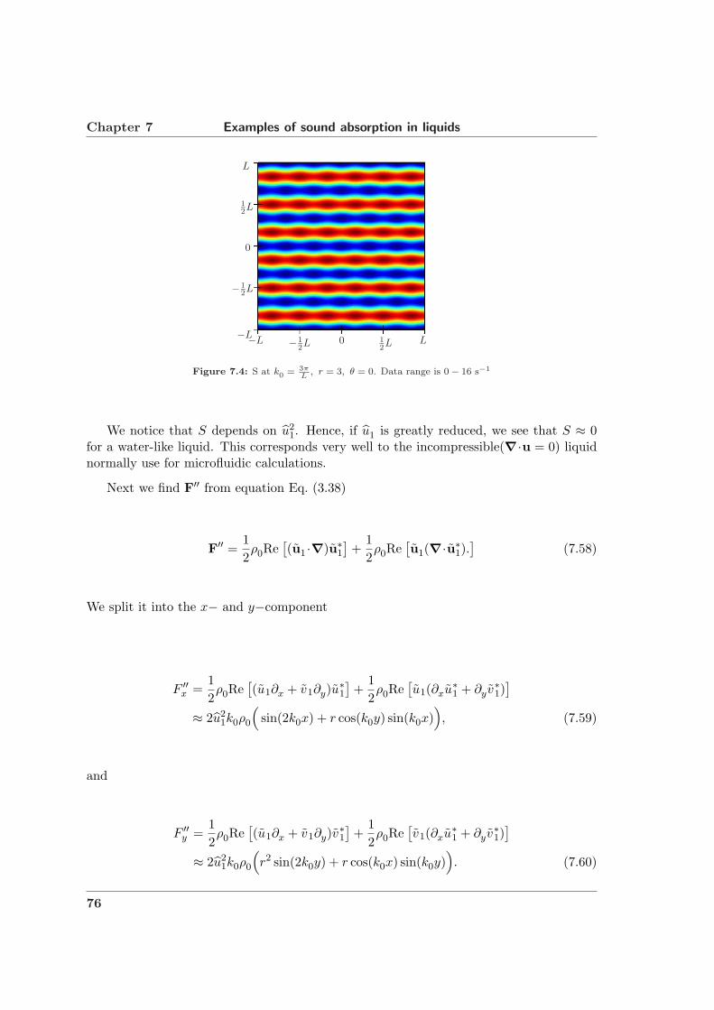
Chapter 7 Examples of sound absorption in liquids
L1
2L0
−
1
2L−L
L
1
2L
0
−
1
2L
−L
Figure 7.4: S at k0 = 3πL
, r = 3, θ = 0. Data range is 0− 16 s−1
We notice that S depends on u21. Hence, if u1 is greatly reduced, we see that S ≈ 0
for a water-like liquid. This corresponds very well to the incompressible(∇·u = 0) liquidnormally use for microfluidic calculations.
Next we find F′′ from equation Eq. (3.38)
F′′ =12ρ0Re
[(u1 ·∇)u∗1
]+
12ρ0Re
[u1(∇·u∗1).
](7.58)
We split it into the x− and y−component
F ′′x =
12ρ0Re
[(u1∂x + v1∂y)u
∗1
]+
12ρ0Re
[u1(∂xu∗1 + ∂yv
∗1)
]
≈ 2u21k0ρ0
(sin(2k0x) + r cos(k0y) sin(k0x)
), (7.59)
and
F ′′y =
12ρ0Re
[(u1∂x + v1∂y)v
∗1
]+
12ρ0Re
[v1(∂xu∗1 + ∂yv
∗1)
]
≈ 2u21k0ρ0
(r2 sin(2k0y) + r cos(k0x) sin(k0y)
). (7.60)
76

Numeric Example 3: Wave resonance, 2D Section 7.3
L1
2L0
−
1
2L−L
L
1
2L
0
−
1
2L
−LL1
2L0
−
1
2L−L
L
1
2L
0
−
1
2L
−L
(a) (b)
Figure 7.5: Panel (a) shows F ′′x and panel (b) shows F ′′y , both at k0 = 3πL
, r = 3, θ = 0. The data range in panel
(a) is ±5× 10¹¹ N m−3, while 9 (r2) times larger in panel (b)
Now that S and F′′ have been calculated, we can use COMSOL to solve the threecoupled partial differential equations numerically(see Appendix D). In this model we cansafely state that the flux normal to any boundary must be zero, as we have non-porouswalls. On the other hand, it is not obvious what conditions we can assume parallel tothe walls, as these are oscillating. But if we have a water-like liquid, we see that thecharacteristic length scale of momentum diffusion is LD =
√η
ρ0ω = 1 µm, which is much
smaller than the element size, used in the numerical calculations. This means that themodel should not be sensitive to small changes in the boundary conditions. Hence, wechoose a neutral boundary condition; we assume the viscous stress is zero. These conditionsare implemented using the method from Section 5.2 by setting
R =Rp′′2 , Ru′′2 , Rv′′2 = 0, J ′′2,x, 0G =Gp′′2 , Gu′′2 , Gv′′2 = 0, 0, 0 (7.61)
for the vertical walls and
R =Rp′′2 , Ru′′2 , Rv′′2 = 0, 0, J ′′2,yG =Gp′′2 , Gu′′2 , Gv′′2 = 0, 0, 0 (7.62)
for the horizontal walls.
The numerical results for u′′2, v′′2 and p′′2 are shown below.
77

Chapter 7 Examples of sound absorption in liquids
L1
2L0
−
1
2L−L
L
1
2L
0
−
1
2L
−LL1
2L0
−
1
2L−L
L
1
2L
0
−
1
2L
−LL1
2L0
−
1
2L−L
L
1
2L
0
−
1
2L
−L
(a) (b) (c)
Figure 7.6: Numeric results from COMSOL for k0 = 3πL
, r = 3, θ = 0. Panel (a) and (b) shows u′′2 and v′′2 ,
respectively. Panel (c) shows p′′2 . The data range in both panel (a) and (b) is ±2.5 × 10⁶ m s−1. The data rangefor panel (c) is 0− 5× 10⁸ Pa.
Again, we notice that the amplitude of several million meters per second is far to high.In Chapter 8 we shall non the less try to compare these results with those experimentallyobtained.
78

Chapter 8
Comparing theory and experiments
As mentioned earlier, we have a huge problem regarding the amplitudes of all the fieldsinvolved in this calculation. But by normalizing the numeric results, their relative valuescan still be compared to those from the experiments.
8.1 Simulated streaming patterns
By plotting the numeric results for u′′2 and v′′2 in a vector plot we can still compare theresulting flow-pattern. In Fig. 8.1 panel (a) we see that a pattern of 6 × 6 vortices hasappeared. We notice that this pattern is very similar to that obtained during the exper-iments, Panel (b). The frequency corresponding to the k0 = nπ
L = 3π0.001m−1 resonance
is 2.2245 MHz. For the corresponding experiment (Fig. 8.1 panel (b)) the frequency wasapproximately 2.17 MHz. Panel (c) shows the result of a calculation performed at thek0 = nπ
L = π0.001m−1 resonance with a frequency at 0.74 MHz. This 2× 2 vortex pattern
was also observed experimentally, at 0.76 MHz. Even though the experimental data shownin panel (d) does not show four complete vortices, it is so close that we assume the correctstate has been found. The lack of uniformity in the experimental data, might by causedby asymmetries in the chip itself or in the entire experimental setup.
79

Chapter 8 Comparing theory and experiments
L1
2L0
−
1
2L−L
L
1
2L
0
−
1
2L
−L
L1
2L0
−
1
2L−L
L
1
2L
0
−
1
2L
−L
(a) (b)
(c) (d)
Figure 8.1: Comparison of vector-plots of the calculated velocities to the PIV-pictures of the experimental velocitiesof the small particles. Panel(a) shows a pattern of 6×6 vortices found at the k0 = 3π/L resonance(2.2 MHz). Panel(b) shows the flow-pattern found at 2.17 MHz. We notice that the predicted 6x6-vortices were indeed observed,and since the experiment were made with small particles they are not noticeably affected by the radiation force.Panel(c) shows a pattern of 2 × 2 vortices found at the k0 = π/L resonance(0.74 MHz). Panel (b) shows theflow-pattern found at 0.76 MHz for small particles. We notice that the predicted 2× 2-vortices also were observed.PIV-pictures(panel (b) and (d)) courtesy Melker Sundin.
The velocity observed in the experiments corresponds to u1 ≈ ω` ≈ 0.001 m/s werethe calculations were performed with u1 ≈ 87 m/s as predicted in Section 4.4.2.
80

Simulated radiation force Section 8.2
8.2 Simulated radiation force
If we turn to look at the acoustic radiation force acting on a particle, we find the expressionfrom Eq. (6.4)
F′′ar = −τp′′2∇p′′2 (8.1)
By plotting the normalized acoustic radiation force we can see that the correspondingbead pattern corresponds very well to the experimental bead pattern.
L1
2L0
−
1
2L−L
L
1
2L
0
−
1
2L
−L
(a) (b)
Figure 8.2: We see that the larger particles were observed to accumulate where the theory predicts.
By assuming the particle motion can be described by a quasi-stationary steady stateflow, we can express the particle velocity as proportional to the acoustic radiation force.Hence, if both are normalized they become identical. Fig. 8.3 shows the experimen-tally measured bead velocity in the y-direction for x = ±L/3. Due to symmetry they-component of the theoretically radiation force is the same for x = ±L/3. Hence, onlyone line represents Far,y
81
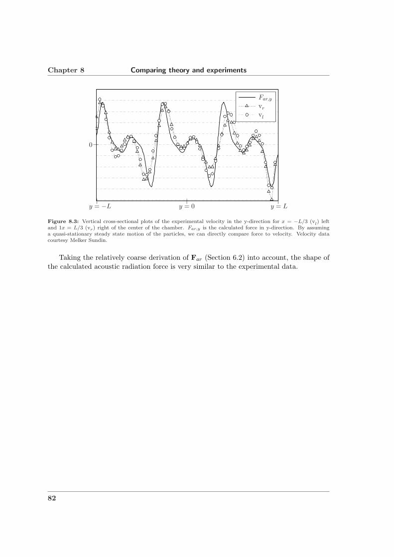
Chapter 8 Comparing theory and experiments
Far,y
vr
vl
y = −L y = 0 y = L
0
Figure 8.3: Vertical cross-sectional plots of the experimental velocity in the y-direction for x = −L/3 (vl) leftand 1x = L/3 (vr) right of the center of the chamber. Far,y is the calculated force in y-direction. By assuminga quasi-stationary steady state motion of the particles, we can directly compare force to velocity. Velocity datacourtesy Melker Sundin.
Taking the relatively coarse derivation of Far (Section 6.2) into account, the shape ofthe calculated acoustic radiation force is very similar to the experimental data.
82

Chapter 9
Conclusion
In Chapter 2 it has been shown that the assumption of oscillating walls surrounding anincompressible liquids, is not sufficient to explain how relatively strong flow patterns canexist far from the boundary. However, by comparing analytical solutions to numericalsolution, we have confirmed that the perturbation method is an acceptable approach forthis kind of system.
The realization that the no-slip condition actually applies to the flux and not onlyto the velocity of a compressible liquid, must be emphasized, as the lack of this (in thehindsight) obvious statement caused some huge problems in the early development of thiswork.
In Chapter 6 it is shown that the nodal-lines in solutions to a eigen-frequency analysisof the pressure-based Helmholtz equation, provide a very accurate hint to were suspendedbeads will eventually accumulate. If the location of the nodal-lines is combined withthe gradient of the corresponding first-order pressure field, one can estimate the relativestrength of acoustic radiation force. It is also shown that as long as the acoustic wave-lengths are more than twice the length of a dimension, the dimension can be omitted fromthe eigen-frequency analysis and the result will still be reasonably accurate.
From the comparisons in Chapter 8 it can be seen that the expression derived in Sec-tion 6.2 for the acoustic radiation force is very useful. The expression can not only accountfor where the particles will accumulate, but it also tells where they will collect fastest, andfinally it gives a reasonable argument to why small particles seems unaffected(Far ∝ r4).
However, from the apparently un-physically high amplitudes calculated, we are lead tothe conclusion that the derivation of the resonance amplitudes in Section 4.4.2 is flawed.One can argue if it is the oscillation amplitude of walls that has been estimated to be toohigh(1 nm) or if the damping in the system is artificially low. Perhaps it is necessary toinclude a loss because of heating.
In Chapter 8 it can be seen the equations developed in Chapter 3 are able to explainthe experimentally observed flow patterns, though again the amplitudes were far to high.
Hence, it can be concluded that the main contributions to the acoustic radiation forceand to acoustic streaming have been understood, with the exception of the amplitudes atresonance-frequencies.
83


Chapter 10
Outlook
To improve the work presented in this thesis, it is obvious that the theory for the attenuatedresonating waves most be remodeled. To validate the results in this thesis, it must beexplained why the particle velocity amplitude is much lower than assumed. To supportany new theory it would be a huge advantage to perform experimental measurements ofsome of the properties (u1, p1, p′′2 etc.) on carefully designed symmetric chips. This wouldease the process when comparing simulations and experiments.
Another interesting aspect to investigate, would be whether the approach used forfinding flow-patterns in the square chamber, can directly be used for the round chamber.
It would also be interesting to derive the acoustic radiation force in greater detail, andhopefully find an expression for the absolute force and not only the relative.
To calculate the the flow-patterns for any given geometry and resonance frequency, itmight be necessary to develop a method to extract the first order terms from the eigen-frequency analysis. By doing so it would not be necessary to guess the strength andphase-shift for each oscillating wall.
Finally the consequences of assuming that all the materials used are isotropic, whenwe know the that the speed of sound in silicon is highly lattice dependant, should beinvestigated.
85


Appendix A
COMSOL-script; Periodic motion in incompressibleliquids
This appendix contains the COMSOL-script use to obtain the numerical solution in Sec-tion 2.4. The script is compiled for COMSOL ver. 3.2
COMSOL1 % Cleaning up
2 clc;close all;clear;flclear fem
3
4 % Definig the Constants
5 PE = 1e-9; % Piezo Expansion, 1nm
6 Pd = 2*pi*1e-6; % Piezo distance,
7 qq =2*pi/Pd; % wavenumber
8 ee = 1; % Becomes Pe
9 w = 2*pi*1e6*ee; % Angular frequency
10 frek = w/(2*pi); % Frequency
11 vv0 = frek*PE; % Slip velocity
12 Tp = 1/frek; % time of one period
13 n = 15; % number of cycles, endtime = n*Tp
14 Ntrans = 10; % number of cycles to be discarded (transient)
15 nt = 100; % number of timesteps per cycle
16 int =Tp/nt; % time interval
17 smesh = Pd/25; % mesh size
18
19 % Introducing the Constants to COMSOL
20 fem.const = ’bl’,Pd,’q’,qq,’eta’,’1e-3’,’rho’,’1e3’,’f’,frek,’v0’,vv0, ...
21 ’w’,w,’epss’,’rho*w/(eta*q^2)’,’Re’,’rho*v0/(q*eta)’;
22
23 % Creating geometry
24 g1=square2(’bl’,’base’,’corner’,’pos’,’0’,’0’,’rot’,’0’,’const’,fem.const);
25 s.objs=g1;
26 s.name=’SQ1’;
27 s.tags=’g1’;
28 fem.draw=struct(’s’,s);
29 fem.geom=geomcsg(fem);
30
31 % Initialize mesh
32 fem.mesh=meshinit(fem,’hgrad’,1.025,’hmaxedg’,[2,smesh]);
33
34 % Application mode 1
87

Appendix ACOMSOL-script; Periodic motion in incompressible liquids
35 clear appl
36 appl.mode.class = ’FlNavierStokes’;
37 appl.gporder = 4,2;
38 appl.cporder = 2,1;
39 appl.assignsuffix = ’_ns’;
40 clear pnt
41 pnt.pnton = 0,1;
42 pnt.ind = [1,2,1,1];
43 appl.pnt = pnt;
44 clear bnd
45 bnd.u0 = 0,’v0*cos(q*x)*sin(w*t)’,0;
46 bnd.type = ’noslip’,’uv’,’neutral’;
47 bnd.ind = [3,2,1,3];
48 appl.bnd = bnd;
49 clear equ
50 equ.init = 0;0;0;
51 equ.rho = ’rho’;
52 equ.eta = ’eta’;
53 equ.cporder = 1;1;2;
54 equ.gporder = 1;1;2;
55 equ.ind = [1];
56 appl.equ = equ;
57 fem.appl1 = appl;
58 fem.border = 1;
59 fem.units = ’SI’;
60
61 % Coupling variable elements
62 clear elemcpl
63 % Extrusion coupling variables
64 clear elem
65 elem.elem = ’elcplextr’;
66 elem.g = ’1’;
67 src = cell(1,1);
68 clear bnd
69 bnd.expr = ,’u’,,’v’,,’p’;
70 bnd.map = ’0’,’0’,’0’;
71 bnd.ind = ’1’,’2’,’3’,’4’;
72 src1 = ,bnd,;
73 elem.src = src;
74 geomdim = cell(1,1);
75 clear bnd
76 bnd.map = ,’1’,,’1’,,’1’;
77 bnd.ind = ’2’,’3’,’4’,’1’;
78 geomdim1 = ,bnd,;
79 elem.geomdim = geomdim;
80 elem.var = ’pconstr1’,’pconstr2’,’pconstr3’;
81 map = cell(1,1);
82 clear submap
83 submap.type = ’linear’;
84 submap.sg = ’1’;
85 submap.sv = ’1’,’2’;
86 submap.dg = ’1’;
87 submap.dv = ’3’,’4’;
88 %submap.dv = ’9’,’10’;
88
Section A.0
89 map1 = submap;
90 elem.map = map;
91 elemcpl1 = elem;
92 % Point constraint variables (used for periodic conditions)
93 clear elem
94 elem.elem = ’elpconstr’;
95 elem.g = ’1’;
96 clear bnd
97 bnd.constr = ’pconstr1-(u)’,’pconstr2-(v)’,’pconstr3-(p)’;
98 bnd.cpoints = ’2’,’2’,’1’;
99 bnd.ind = ’1’;
100 elem.geomdim = ,bnd,;
101 elemcpl2 = elem;
102 fem.elemcpl = elemcpl;
103
104 % Solve problem
105 fem=multiphysics(fem);
106 fem.xmesh=meshextend(fem);
107 fem.sol=femtime(fem, ...
108 ’solcomp’,’u’,’p’,’v’, ...
109 ’outcomp’,’u’,’p’,’v’, ...
110 ’tlist’,[0:int:n*Tp], ... %Give output at these time-steps
111 ’atol’,’1e-10’, ...
112 ’rtol’,0.001, ...
113 ’estrat’,1, ...
114 ’tout’,’tlist’);
115
116 % Save parameter in fem structure
117 fem.tgj.n = n;
118 fem.tgj.Ntrans = Ntrans;
119 fem.tgj.nt = nt;
120 fem.tgj.v0 = vv0;
121 fem.tgj.int = int;
122 fem.tgj.smesh = smesh;
123 fem.tgj.epss=postint(fem,’epss’, ’dl’,[3],’edim’,0);
124 fem.tgj.Re=postint(fem,’Re’,’dl’,[3], ’edim’,0);
125
126 % Calculating the time-averaged solution
127 femsolu=fem.sol.u;
128 SIZEU=size(femsolu);
129 r = SIZEU(1);
130 s = SIZEU(2);
131 U = zeros(r,1);
132 k =fem.tgj.Ntrans*fem.tgj.nt;
133 for i = k:s % Sum up solutions, without transint
134 U = U + femsolu(:,i);
135 end
136 U = U./(s-k);
137 fem.tgj.avgU = U;
138
139 % Find Absolute Average Velocity
140 U = fem.tgj.avgU;
141 int = postint(fem,’(U_ns^2)^0.5’,’U’,U,’dl’,[1]); %use U as input (not fem)
142 fem.tgj.INT_ER = int/(Pd*Pd)
89

Appendix ACOMSOL-script; Periodic motion in incompressible liquids
143
144 % Investigate the transient
145 figure
146 SIZEU = size(fem.sol.u);
147 r = SIZEU(1);
148 s = SIZEU(2);
149
150 field = 2251;
151 p = round(fem.tgj.nt);
152 for i=1:s
153 i/s
154 u(i)=postint(fem,’u’,’dl’,[3],’solnum’,i,’edim’,0);
155 t(i) = fem.sol.tlist(i);
156 end
157
158 t0 = 2; % Two random timesteps
159 t1 = 8;
160 plot(t(t1:p:end),u(t1:p:end),’r-’),hold on
161 plot(t(t1:p:end),u(t1:p:end),’ro’),hold on
162 plot(t(t0:p:end),u(t0:p:end),’ro’),hold on
163 plot(t(t0:p:end),u(t0:p:end),’r-’),hold on
164
165 bc = -sin(fem.tgj.n*2*pi*(fem.sol.tlist)./fem.sol.tlist(end)’)/1e6;
166
167 plot(t,bc,’k:’),hold on
168 plot(t,u,’b-’),hold on
169 plot(t,u,’bx’)
170
171 % Plot Averaged solution
172 figure
173 %fem.xmesh=meshextend(fem);
174
175 postplot(fem,’tridata’,’u’,’cont’,’internal’, ...
176 ’trimap’,’jet(1024)’, ...
177 ’U’,fem.tgj.avgU,...
178 ’arrowdata’,’u’,’v’, ...
179 ’arrowxspacing’,30, ...
180 ’arrowyspacing’,30, ...
181 ’arrowtype’,’arrow’, ...
182 ’arrowstyle’,’proportional’, ...
183 ’arrowcolor’,[1.0,0.0,0.0], ...
184 ’solnum’,1, ...
185 ’title’,[’Time-averaged velocity - first ’, num2str(10),’ periods discarded’], ...
186 ’refine’,3);COMSOL
90

Appendix B
COMSOL-script; Wave propagation throughinterfaces
This appendix contains the COMSOL-script use to obtain the numerical solution in Sec-tion 4.3. The script is compiled for COMSOL ver. 3.2
COMSOL1 % Cleaning up
2 clear,flgc,clc,flclear fem
3
4 % Constants
5 fem.const = ’f’,’5.6887e6’,’w’,’2*pi*f’;
6
7 % Geometry
8 clear draw
9 g1=rect2(0,300e-6,0,10e-6);
10 g2=rect2(300e-6,500e-6,0,10e-6);
11 g3=rect2(500e-6,1000e-6,0,10e-6);
12 g4=rect2(1000e-6,1200e-6,0,10e-6);
13 draw.s.objs = g1,g2,g3,g4;
14 fem.draw = draw;
15 fem.geom = geomcsg(fem);
16
17 % Create mapped quad mesh
18 MeshFactor = 30;
19 fem.mesh=meshmap(fem,’edgelem’,2,[3*MeshFactor],...
20 3,[3*MeshFactor],...
21 5,[2*MeshFactor],...
22 6,[2*MeshFactor],...
23 8,[5*MeshFactor],...
24 9,[5*MeshFactor],...
25 11,[2*MeshFactor],...
26 12,[2*MeshFactor]);
27
28 % Application mode 1
29 clear appl
30 appl.mode.class = ’Acoustics’;
31 appl.assignsuffix = ’_aco’;
32 clear bnd
33 bnd.type = ’NA’,’SH’,’cont’,’IMP’;
34 bnd.nacc = ’-i*w^2*1e-9’,0,0,0;
91

Appendix B COMSOL-script; Wave propagation through interfaces
35 bnd.Z = ’0’,’0’,’0’,’343.4*1.161’;
36 bnd.ind = [1,2,2,3,2,2,3,2,2,3,2,2,4];
37 appl.bnd = bnd;
38 clear equ
39 equ.cs = 8490,1483,5640,343.4;
40 equ.rho = 2331,998.2,2230,1.161;
41 equ.ind = [1,2,3,4];
42 appl.equ = equ;
43 appl.var = ’freq’,’f’;
44 fem.appl1 = appl;
45 fem.border = 1;
46 fem.units = ’SI’;
47
48 % Solve problem
49 fem=multiphysics(fem);
50 fem.xmesh=meshextend(fem);
51 fem.sol=femlin(fem,’solcomp’,’p’, ...
52 ’outcomp’,’p’);
53
54 % Plot cross-section along all domains
55 postcrossplot(fem,1,[0 0.0012;0 0], ...
56 ’lindata’,’p*exp(i*w*(0.6/f))’, ...
57 ’axis’,[0 1200e-6]);COMSOL
92

Appendix C
COMSOL-script; The symmetric chamber model
This appendix contains the COMSOL-script use to obtain the numerical solution in Sec-tion 6.4. The script is compiled for COMSOL ver. 3.2
COMSOL1 % Cleaning up
2 clc;close all;flclear fem
3
4 % Constants
5 k = 8; %number of eigenvalues to be found
6 startF =2.2e6; %where to start eigenvalue search
7 CorS = 1; %0=circle-geom, 1=square-geom
8
9 % Geometry
10 g1=rect2(’0.025’,’400e-6’,’base’,’center’,’pos’,’0’,’0’,’rot’,’0’);
11 if CorS <=0.5
12 g2=circ2(’1e-3’,’base’,’center’,’pos’,’0’,’0’,’rot’,’0’);
13 elseif CorS >= 0.49
14 g2=square2(’2e-3’,’base’,’center’,’pos’,’0’,’0’,’rot’,’0’);
15 else
16 k=1;
17 disp(’CorS - Error’)
18 end
19 g3=geomcomp(g1,g2,’ns’,’g1’,’g2’,’sf’,’g1+g2’,’edge’,’none’);
20 g4=geomdel(g3);
21 clear s
22 s.objs=g4;
23 s.name=’CO2’;
24 s.tags=’g4’;
25 fem.draw=struct(’s’,s);
26 fem.geom=geomcsg(fem);
27
28 % Initialize mesh
29 fem.mesh=meshinit(fem,’hmax’,[50e-6]);
30
31 % Application mode 1
32 clear appl
33 appl.mode.class = ’Acoustics’;
34 appl.assignsuffix = ’_aco’;
35 clear prop
36 prop.analysis=’eigen’;
93

Appendix C COMSOL-script; The symmetric chamber model
37 appl.prop = prop;
38 clear bnd
39 bnd.type = ’SH’,’SS’;
40 if CorS <=0.5
41 bnd.ind = [2,1,1,1,1,2,1,1,1,1];
42 elseif CorS >= 0.49
43 bnd.ind = [2,1,1,1,1,1,1,1,1,1,1,2];
44 else
45 k=1;
46 disp(’CorS - Error’)
47 end
48 appl.bnd = bnd;
49 clear equ
50 equ.cs = 1483;
51 equ.rho = 998.2;
52 equ.ind = [1];
53 appl.equ = equ;
54 fem.appl1 = appl;
55 fem.border = 1;
56 fem.units = ’SI’;
57
58 % Solve problem
59 fem=multiphysics(fem);
60 fem.xmesh=meshextend(fem);
61 fem.sol=femeig(fem,’solcomp’,’p’, ...
62 ’outcomp’,’p’, ...
63 ’neigs’,k, ...
64 ’shift’,(2*pi*startF)^2); %Start search here
65
66 % Plot the found solutions
67 for i=1:k
68 w=fem.sol.lambda(i);
69 F = w^0.5/(2*pi);
70 figure(’position’, [100, 100, 1201, 900])
71 subplot(’position’, [0, 0, 1, 1])
72 postplot(fem, ...
73 ’tridata’,’p’,’cont’,’internal’, ...
74 ’trimap’,’jet(1024)’, ...
75 ’tribar’,’off’,...
76 ’tridlim’,[-2,2], ...
77 ’solnum’,i, ...
78 ’refine’,3);
79 axis off
80 disp([i F])
81 endCOMSOL
94

Appendix D
COMSOL-script; Numeric Example 3
This appendix contains the COMSOL-script use to obtain the numerical solution in Sec-tion 7.3. The script is compiled for COMSOL ver. 3.2
COMSOL1 % Cleaning up
2 close all,clear fem,flclear fem,flgc,clc
3
4 % GEOMETRY
5 L=0.001;
6 fem.geom = rect2(-L,L,-L,L)+point2(-L/6,-L/6);
7 fem.mesh = meshinit(fem);
8
9 % Mesh
10 sm=0.25e-4;
11 bm=sm;
12 fem.mesh=meshinit(fem,’hmaxedg’,[1,bm,2,bm,3,bm,4,bm], ...
13 ’hmaxsub’,[1,sm]);
14
15 % Space dimension
16 fem.sdim = ’x’ ’y’;
17
18 % Dependent variables
19 fem.dim = ’u’ ’v’ ’p’;
20 fem.shape = [2 2 1];
21
22 % Constants
23 fem.const = ’k’,’n*pi/L’, ...
24 ’n’,’3’, ...
25 ’c’,’1483’, ...
26 ’th’,’0’, ... %theta
27 ’r’,’3’, ...
28 ’epss’,’w*l/c’, ...
29 ’l’,’1e-9’, ...
30 ’bl’,’2*L/n’, ...
31 ’f’,’c/bl’, ...
32 ’w’,’2*pi*f’, ...
33 ’L’,L, ...
34 ’rho’,’998.2’, ...
35 ’ga’,’(beta+1)*w*eta/(2*rho*c^2)’, ... %gamma
36 ’beta’,’5/3’, ...
95

Appendix D COMSOL-script; Numeric Example 3
37 ’eta’,’1e-3’,...
38 ’uhat’,’-epss*c/(2*n*pi*gamma)’;
39
40 fem.expr =
41 ’sigmaxx’ ’-p+(beta+1)*eta*ux’ ...
42 ’sigmaxy’ ’eta*(uy+beta*vx)’ ...
43 ’sigmayx’ ’eta*(vx+beta*uy)’ ...
44 ’sigmayy’ ’-p+(beta+1)*eta*vy’, ...
45 ’S’,’(2*uhat^2*w*ga/(c^2))*(1+r^2-cos(2*k*x)-r^2*cos(2*k*y))’, ...
46 ’Fx1’,’(2*uhat^2*w*rho/c^2)’, ...
47 ’Fx2’,’(c*sin(2*k*x)+ga*r*w*y*sin(k*x)*sin(k*y)*sin(th))’, ...
48 ’Fx3’,’(r*cos(k*y)*(c*cos(th)*sin(k*x)+ga*(w*x*cos(k*x)-c*sin(k*x))*sin(th)))’, ...
49 ’Fx’,’Fx1*(Fx2+Fx3)’, ...
50 ’Fy1’,’(2*uhat^2*w*rho*r^2/c^2)’, ...
51 ’Fy2’,’(c*r*sin(2*k*y)-ga*w*x*sin(k*x)*sin(k*y)*sin(th))’, ...
52 ’Fy3’,’(cos(k*x)*(c*cos(th)*sin(k*y)+ga*(-w*y*cos(k*y)+c*sin(k*y))*sin(th)))’, ...
53 ’Fy’,’Fy1*(Fy2+Fy3)’, ...
54 ’tp1u1a’,’-2*ga*r*w*x*cos(k*x)*cos(k*y)*cos(th)’,...
55 ’tp1u1b’,’+ga*(c*sin(2*k*x)-2*w*(x+r*y*cos(th)*sin(k*x)*sin(k*y)))’,...
56 ’tp1u1’,’uhat^2*rho*(tp1u1a+tp1u1b+2*c*r*cos(k*y)*sin(k*x)*(ga*cos(th)+sin(th)))’, ...
57 ’tp1v1a’,’r*y*ga*w+w*x*ga*cos(th)*sin(k*x)*sin(k*y)-1/2*c*r*ga*sin(2*k*y)’, ...
58 ’tp1v1b’,’cos(k*x)*(w*y*ga*cos(k*y)*cos(th)+c*sin(k*y)*(-ga*cos(theta)+sin(th)))’, ...
59 ’tp1v1’,’-2*uhat^2*r*rho*(tp1v1a+tp1v1b)’, ...
60 ’J2X’,’rho*u+tp1u1/c^2’, ...
61 ’J2Y’,’rho*v+tp1v1/c^2’
62 ;
63
64 % Governing equations
65 fem.form = ’general’;
66 fem.equ.ga = ’sigmaxx’ ’sigmaxy’ ’sigmayx’ ’sigmayy’ ’0’ ’0’;
67 fem.equ.f = ’Fx’ ’Fy’ ’ux+vy-S’;
68
69 % Boundary conditions
70 fem.bnd.ind = [1 4] [2 3];
71 fem.bnd.r = ’J2X’ ’0’ ’0’ ’0’ ’J2Y’ ’0’;
72 fem.pnt.constr = 0,0;0;’p’;
73 fem.pnt.ind = [1,1,2,1,1];
74
75 % Solve problem
76 fem.xmesh = meshextend(fem);
77 fem.sol = femnlin(fem,’report’,’on’);
78
79 % Plot solution
80 postplot(fem, ...
81 ’tridata’,’p’,’cont’,’internal’, ...
82 ’trimap’,’jet(1024)’, ...
83 ’refine’,3);COMSOL
96

Bibliography
[1] J. Lighthill, Waves in Fluids (Cambridge University Press, Cambridge, 2005), 3 edi-tion.
[2] T. Duke and R. Austin, ‘Microfabricated sieve for the continuous sorting of macro-molecules’, Physical Review Letters 80, 1552 (1998).
[3] W. Yi-zhong and Z. Zhan, ‘Biochip development and improvement based on elec-trophoresis separation’, Instrument Techniques and Sensor 6–22 (2006).
[4] W. A. Mac Crehan, H. T. Rasmussen, and D. M. Northrop, ‘Size-selective capillaryelectrophoresis (SSCE) separation of dna fragments’, Journal of Liquid Chromatog-raphy 15, 1063 (1992).
[5] B. Biscans and J. Bertrand, ‘ELECTROPHORETIC SEPARATIONS - MOD-ELLING OF THE TRANSIENT STATE OF THE BUFFER SOLUTION FLOW.’,Chemical Engineering Research And Design 65, 224 (1987).
[6] F. Aldaeus, Y. Lin, G. Amberg, and J. Roeraade, ‘Multi-step dielectrophoresis forseparation of particles’, Journal of Chromatography A 1131, 261 (2006).
[7] D. Chen, H. Du, and W. Li, ‘Bioparticle separation and manipulation using dielec-trophoresis’, Sensors & Actuators: A. Physical 133, 329 (2007).
[8] Y. Jing, L. R. Moore, P. S. Williams, J. J. Chalmers, S. S. Farag, B. Bolwell, andM. Zborowski, ‘Blood progenitor cell separation from clinical leukapheresis productby magnetic nanoparticle binding and magnetophoresis’, Biotechnology and Bioengi-neering 96, 1139 (2007).
[9] N. Pamme and C. Wilhelm, ‘Continuous sorting of magnetic cells via on-chip free-flow magnetophoresis’, Lab on a Chip 6, 974 (2006).
[10] L. King, ‘Acoustic radiation pressure on circular discs: inertia and diffraction cor-rections’, Proceedings of the Royal Society of London 153A (1935).
[11] Y. K. K. Yosika, ‘Acoustic Radiation Pressure On A Compressible Sphere’, Acustica5, 167 (1955). Institute of Scientific and Industrial Research, Osaka University.
[12] A. Haake and J. Dual, ‘Micro-manipulation of small particles by node position controlof an ultrasonic standing wave’, Ultrasonics 40, 317 (2002).
97

Bibliography
[13] D.-H. Kim, A. Haake, Y. Sun, A. Neild, J.-E. Ihm, J. Dual, J. Hubbell, B.-K. Ju, andB. Nelson, ‘High-throughput cell manipulation using ultrasound fields’, Engineeringin Medicine and Biology Society, 2004. EMBC 2004. Conference Proceedings. 26thAnnual International Conference of the 1, 2571 (2004).
[14] L. A. Kuznetsova and W. T. Coakley, ‘Microparticle concentration in short path lengthultrasonic resonators: Roles of radiation pressure and acoustic streaming’, Journal ofthe Acoustical Society of America 116, 1956 (2004).
[15] K. Yasuda, S.-I. Umemura, and K. Takeda, ‘Concentration and fractionation of smallparticles in liquid by ultrasound’, Japanese Journal of Applied Physics, Part 1 (Reg-ular Papers and Short Notes) 34, 2715 (1995).
[16] A. Nilsson, F. Petersson, H. Jonsson, and T. Laurell, ‘Acoustic control of suspendedparticles in micro fluidic chips’, Lab on a Chip 4, 131 (2004).
[17] H. Li and T. Kenny, ‘High speed particles separation using ultrasound for microTASand lab-on-a-chip application’, Proceeding of the 26th Annual International Confer-ence of the IEEE EMBS 3, 2631 (2004).
[18] H. Jonsson, C. Holm, A. Nilsson, F. Petersson, P. Johnsson, and T. Laurell, ‘Parti-cle Separation Using Ultrasound Can Radically Reduce Embolic Load to Brain AfterCardiac Surgery’, The Annals of Thoracic Surgery 78, 1572 (2004).
[19] A. Hatch, E. Garcia, and P. Yager, ‘Diffusion-based analysis of molecular interactionsin microfluidic devices’, Proceedings of the IEEE 92, 126 (2004).
[20] F. Bottausci, C. Cardonne, C. Meinhart, and I. Mezic, ‘An ultrashort mixing lengthmicromixer: The shear superposition micromixer’, Lab on a Chip 7, 396 (2007).
[21] S.-Y. Jin, Y.-Z. Liu, W.-Z. Wang, Z.-M. Cao, and H. S. Koyama, ‘Numerical evalua-tion of two-fluid mixing in a swirl micro-mixer’, Journal of Hydrodynamics 18, 542(2006).
[22] C.-H. Lin, C.-H. Tsai, C.-W. Pan, and L.-M. Fu, ‘Rapid circular microfluidic mixerutilizing unbalanced driving force’, Biomedical Microdevices 9, 43 (2007).
[23] S. Wang, H. Chen, C. Lee, C. Yu, and H. Chang, ‘AC electro-osmotic mixing inducedby non-contact external electrodes’, Biosensors and Bioelectronics 22, 563 (2006).
[24] C. Eckart, ‘Vortices and streams caused by sound waves’, Physical Review 73, 68(1948).
[25] J. Markham, ‘Second order acoustic fields: streaming with viscosity and relaxation’,Physical Review 86 (1952).
[26] W. Nyborg, ‘Acoustic streaming due to attenuated plane waves’, Journal of the Acous-tical Society of America 25 (1953).
98

Bibliography
[27] http://www.smartbiomems.com.
[28] Handbook of Chemistry and Physics Online (CRC Press, 2006-2007), 87th edition.http://www.hbcpnetbase.com/
[29] NIST - Data Gateway (National Institute of Standards and Technology, 2004).http://srdata.nist.gov/gateway/
[30] C. Ishiyama and Y. Higo, ‘Effects of humidity on Young’s modulus in poly(methylmethacrylate)’, Journal of Polymer Science, Part B: Polymer Physics 40, 460 (2002).
[31] J. Markham, R. Beyer, and R. Lindsay, ‘Absorption of sound in fluids’, Reviews ofModern Physics 23 (1951).
[32] N. H. Asmar, Partial Differential Equations with Fourier Series and Boundary ValueProblems (Pearson Prentice Hall, 2004), 2 edition.
99