Theory of pressure acoustics with viscous boundary layers andstreaming in curved elastic cavities

Jacob S. Bach and Henrik Bruusa)

Department of Physics, Technical University of Denmark, DTU Physics Building 309, DK-2800 KongensLyngby, Denmark

(Received 22 April 2018; revised 6 July 2018; accepted 20 July 2018; published online 17 August2018)

The acoustic fields and streaming in a confined fluid depend strongly on the viscous boundary layer

forming near the wall. The width of this layer is typically much smaller than the bulk length scale

set by the geometry or the acoustic wavelength, which makes direct numerical simulations chal-

lenging. Based on this separation in length scales, the classical theory of pressure acoustics is

extended by deriving a boundary condition for the acoustic pressure that takes viscous boundary-

layer effects fully into account. Using the same length-scale separation for the steady second-order

streaming, and combining it with time-averaged short-range products of first-order fields, the usual

limiting-velocity theory is replaced with an analytical slip-velocity condition on the long-range

streaming field at the wall. The derived boundary conditions are valid for oscillating cavities of

arbitrary shape and wall motion, as long as both the wall curvature and displacement amplitude are

sufficiently small. Finally, the theory is validated by comparison with direct numerical simulation

in two examples of two-dimensional water-filled cavities: The well-studied rectangular cavity with

prescribed wall actuation, and a more generic elliptical cavity embedded in an externally actuated

rectangular elastic glass block. VC 2018 Acoustical Society of America.

https://doi.org/10.1121/1.5049579

[PLM] Pages: 766–784

I. INTRODUCTION

The study of ultrasound effects in fluids in sub-millimeter

cavities and channels has intensified the past decade, as micro-

scale acoustofluidic devices are used increasingly in biology,

environmental and forensic sciences, and clinical diagnos-

tics.1,2 Examples include cell synchronization,3 enrichment of

prostate cancer cells in blood,4 size-independent sorting of

cells,5 manipulation of C. elegans,6 and single-cell patterning.7

Acoustics can also be used for non-contact microfluidic

trapping and particle enrichment8–10 as well as acoustic

tweezing.11–14

The two fundamental physical phenomena that enable

these microscale acoustofluidic applications are rooted in non-

linear acoustics. One fundamental phenomenon is the acoustic

radiation force, which tends to focus suspended particles in the

pressure nodes based on their acoustic contrast to the surround-

ing fluid.15–21 The second fundamental phenomenon is the

acoustic streaming appearing as steady flow rolls which tend

to defocus suspended particles due to the Stokes drag.22–27

Because the acoustic radiation force scales with the volume of

the suspended particle, and the Stokes drag with its radius, the

former dominates for large particles and the latter for small.

For water at room temperature and 1 MHz ultrasound, the criti-

cal particle radius for the crossover between these two regimes

has been determined to be around 2 lm.28,29

So far, the vast majority of successful microscale acous-

tofluidics applications has been for large (above 2 lm) par-

ticles, such as cells, whose dynamics is dominated by the

well-characterized, robust acoustic radiation force, which

depends on the bulk properties of the acoustic field and

material parameters of the particles and the surrounding

fluid. However, there is a strong motivation to handle also

sub-micrometer particles such as bacteria, exosomes, and

viruses, for use in contemporary lab-on-a-chip-based diag-

nostics and biomedical research.9,30–32 In contrast to large

particles, the dynamics of small (sub-micrometer) particles

is dominated by the drag force from the ill-characterized

acoustic streaming. To control the handling of such nanopar-

ticle suspensions, a deeper understanding of the often com-

plicated acoustic streaming is called for.

One important aspect of ultrasound acoustics is the large

velocity gradients in the sub-micrometer-thin viscous bound-

ary layer near rigid boundaries.22 The shear stress and the

Reynolds stress that build up in this region are responsible

for the viscous damping of the acoustic fields and for the

acoustic streaming, respectively. In water with kinematic

viscosity �0 � 10�6 m2=s at the frequency f ¼ ð1=2pÞx � 1

MHz, the thickness d ¼ffiffiffiffiffiffiffiffiffiffiffiffiffi2�0=x

pof this boundary layer is

on the order of 500 nm, while the acoustic wavelength is

around 1.5 mm. This three-orders-of-magnitude separation

of physically relevant length scales poses a severe challenge

for numerical simulations. To circumvent the problem of

resolving the thin boundary layer, we develop a theory were

analytical solutions for the boundary layers are used to for-

mulate boundary conditions for the pressure field and bulk

streaming field, which both varies on the much longer length

scale d � d.

First, we extend the classical pressure acoustics theory

by formulating a boundary condition for the acoustic pres-

sure that includes the presence of the boundary layer, whicha)Electronic mail: bruus@fysik.dtu.dk

766 J. Acoust. Soc. Am. 144 (2), August 2018 VC 2018 Acoustical Society of America0001-4966/2018/144(2)/766/19/$30.00

is otherwise neglected. Thus, our extended boundary condi-

tion takes into account important effect of the boundary

layer, such as increased viscous damping, shifts in resonance

frequencies, and shear stresses on the surrounding walls.

Second, we formulate a generalized slip-velocity bound-

ary condition for bulk acoustic streaming over curved oscillat-

ing surfaces. An important step in this direction was the

development of the limiting-velocity theory by Nyborg in

1958 for perpendicularly oscillating curved walls.33 Later

modifications of this theory comprise modifications to the

analysis in curvilinear coordinates by Lee and Wang in

1989,34 and the treatment of oscillations in any direction for

flat walls by Vanneste and B€uhler in 2011.35 Here, we extend

these theories to harmonic oscillations in any direction of an

arbitrarily shaped elastic wall, provided that both the radius of

curvature and the acoustic wavelength are much larger than

the boundary layer length-scale d, and that also the amplitude

of the perpendicular surface vibration is much smaller than d.

Notably, the theoretical description developed here

allows us to perform numerical simulations of the linear and

nonlinear acoustics in arbitrarily shaped liquid-filled cavities

embedded in oscillating elastic solids. Examples and valida-

tion of such simulations for two-dimensional (2D) systems

are presented in the final sections of this paper, while a study

of three-dimensional (3D) systems is work in progress to be

presented later.

II. WALL MOTION AND PERTURBATION THEORY

We consider a fluid domain X bounded by an elastic,

oscillating solid, see Fig. 1. All acoustic effects in the fluid

are generated by the fluid-solid interface that oscillates har-

monically around its equilibrium position, denoted s0 or @X,

with an angular frequency x. The instantaneous position

sðs0; tÞ at time t of this interface (the wall), is described by

the small complex displacement s1ðs0Þe�ixt,

sðs0; tÞ ¼ s0 þ s1ðs0Þ e�ixt: (1)

In contrast to Muller and Bruus,36 we do not study the tran-

sient phase leading to this steady oscillatory motion.

A. Fundamental conservation laws in acoustofluidics

The theory of acoustofluidics in X is derived from the

conservation of the fluid mass and momentum density,

@tq ¼ �$ � ðqvÞ; (2a)

@tðqvÞ ¼ �$ � ðqvÞv½ � þ $ � r; (2b)

where q is the mass density, v is the Eulerian fluid velocity,

and r is the viscous stress tensor, given by

r ¼ �p Iþ s; (2c)

s ¼ gb0 $ � vð ÞIþ g0

�$vþ $vð ÞT � 2

3$ � vð ÞI

�:

(2d)

Here, p is the pressure and s is the viscous part of the stress

tensor given in terms of the bulk viscosity gb0, the dynamic

viscosity g0, the identity matrix I, and the superscript “T”

denoting matrix transpose. Thermal dissipation is neglected

throughout this work. We introduce the isentropic compress-

ibility j0 and speed of sound c0,

j0 ¼1

q0

@q@p

� �S

¼ 1

q0c20

; (3)

as well as the small dimensionless damping coefficient C in

terms of the viscosity ratio b,

C ¼ bþ 1ð Þg0xj0; b ¼ gb0

g0

þ 1

3: (4)

B. Perturbation expansion

The linear acoustic response of the system is propor-

tional to the displacement stimulus s1ðs0Þe�ixt, and the

resulting complex-valued quantities Q1ðrÞ e�ixt are called

first-order fields with subscript “1”. The physical time-

dependent quantity Qphys1 ðr; tÞ corresponding to Q1 is given

by the real part Qphys1 ðr; tÞ ¼ Re½Q1ðrÞ e�ixt�.

As the governing equations are nonlinear, we also encoun-

ter higher-order terms, and in the present work, we include

terms to second order in the stimulus. Moreover, since we are

only interested in the steady part of these second-order fields,

we let in the following the subscript “2” denote a time-

averaged quantity, written as Q2ðrÞ ¼ hQ2ðr; tÞi¼ ðx=2pÞ

Ð 2p=x0

Q2ðr; tÞ dt. Time-averages of products of

time-harmonic complex-valued first-order fields A1 and B1 are

also of second order, and for those we have

hA1B1i ¼ 12

Re½A1ðrÞB�1ðrÞ�, where the asterisk denote com-

plex conjugation.

Using this notation for the fluid, we expand the mass

density q, the pressure p, and the velocity v in perturbation

series of the form

q ¼ q0 þ q1ðrÞe�ixt þ q2ðrÞ; (5a)

p ¼ p0 þ p1ðrÞe�ixt þ p2ðrÞ; (5b)

v ¼ 0þ v1ðrÞe�ixt þ v2ðrÞ; (5c)

FIG. 1. (Color online) Sketch of the interface between a fluid (light blue, X)

and a curved, oscillating solid (dark gray) with instantaneous position s(dark green line) and equilibrium position s0 (black line, @X). The local cur-

vilinear coordinate system on the interface is given by the tangent vectors en

and eg and the normal vector ef. By a Helmholtz decomposition, the

first-order acoustic fluid velocity v1 ¼ vd1 þ vd

1 is written as the sum of a

long-range compressible part vd1 (dark blue) extending into the bulk and a

short-range incompressible part vd1 (light red) with a decay length equal to

the boundary-layer width d. V01 ¼ vd0

1 þ vd01 is the Lagrangian velocity of

the interface (the wall).

J. Acoust. Soc. Am. 144 (2), August 2018 Jacob S. Bach and Henrik Bruus 767

where q1 � q0; p1 ¼ c20q1 � c2

0q0, and jv1j � c0. The sub-

scripts 1 and 2 denote the order in the small acoustic Mach

number Ma ¼ ð1=c0Þjv1j, which itself is proportional to s1.

C. No-slip boundary condition at the wall

To characterize the wall motion, we compute the time

derivative of sðs0; tÞ in Eq. (1),

@tsðs0; tÞ ¼ �ixs1ðs0Þ e�ixt ¼ V01ðs0Þ e�ixt; (6)

where V01ðs0Þ ¼ �ixs1ðs0Þ is the Lagrangian velocity of the

wall surface element with equilibrium position s0 and instan-

taneous position s. The no-slip boundary condition on the

Eulerian fluid velocity vðr; tÞ is imposed at the instantaneous

surface position sðtÞ,35,37

vðs0þ s1e�ixt; tÞ¼V01ðs0Þe�ixt; no–slip condition: (7)

Combining Eqs. (5c) and (7) with the Taylor expansion

v1ðs0 þ s1; tÞ � v1ðs0Þe�ixt þhðs1 � $Þv1ijs0, and collecting

the terms order by order, gives

v1ðs0Þ ¼ V01ðs0Þ; 1st–order condition; (8a)

v2ðs0Þ ¼ �hðs1 � $Þv1ijs0; 2nd–order condition: (8b)

Note that the expansion, or Stokes drift, in Eq. (8b) is valid,

if the length scale over which v1 varies is much larger than

js1j. So we require js1kj � d and js1fj � d.

D. The limit of weakly curved, thin boundary layers

The crux of our work is the analytical treatment of

weakly curved, thin viscous boundary layers. This notion is

quantified using the boundary-layer length scale d and the

compressional length scale d,

d ¼ffiffiffiffiffiffiffi2�0

x

r; d ¼ min k�1

0 ;R� �

; (9)

where d is the minimum of the wavelength scale k�10 ¼ c0=x

and the length scale R over which the surface curves. We

express our subsequent analysis to lowest order in �, defined

as the ratio of these length scales,

� ¼ dd� 1; (10)

where the inequality holds in the limit of weakly curved

(d=R� 1), thin boundary layers (k0d� 1), a condition usu-

ally satisfied in microfluidic devices.

E. Local boundary-layer coordinates

The limit �� 1 allows for drastic simplifications of the

otherwise complex analytical expressions for curvilinear

derivatives of fields inside the boundary layers at distances

of order d or smaller from the wall. To see this, we introduce

the local, right-handed, orthogonal, curvilinear coordinate

system with coordinates n, g, and f. The latter measures dis-

tance away from the surface equilibrium position along the

surface unit normal vector ef, while the tangential coordi-

nates n and g increase in the respective directions of the unit

tangent vectors en and eg, but not necessarily measuring arc

length, see Fig. 1. To make the scale R of the curved surface

explicit, we use the vectorial notation for curvilinear deriva-

tives and introduce the differential-geometric symbols

employed in previous boundary-layer analyses in the

literature,33,34

hi ¼ j@irj; Tkji ¼ ~@ kej

� ei; for i; j;k ¼ n;g; f;

~@ i ¼1

hi@i; Hk ¼ Tiki ¼ ~@ k

Xi 6¼k

log hi

� �: (11)

Note that this is not covariant formulation, see Appendix A for

details on the differential geometry. Because f measures arc

length, we have hf ¼ 1 and consequently ~@ f ¼ @f. The surface

length scale can now be defined as R minfT�1kji ;H�1

k g,which in many situations is comparable with the surface curva-

ture radius.

F. Surface fields, boundary-layer fields, and bulk fields

For �� 1, we may separate any field A inside the

boundary layer in the perpendicular coordinate f,

Aðn; g; fÞ ¼ A0ðn; gÞ aðfÞ; f � d� d: (12)

Here, superscript “0” defines a surface field A0ðn; gÞ¼ Aðn; g; 0Þ, such as the wall velocity V0

1 and the fluid veloc-

ity v0 at the equilibrium position s0 of the wall. Note that

a surface field does not have a perpendicular derivative,

although it does have a perpendicular component. This coor-

dinate separation results in the following expressions in

vectorial notation for the divergence (A6) and advective

derivative (A8) involving surface fields:

$ � A0 ¼ $k � A0k þ HfA

0f ; (13a)

ðA0 � $ÞB0 ¼ A0k � ð$kB0

i Þ ei þ A0kB0

j Tkjiei; (13b)

Ak ¼ An en þ Ag eg; (13c)

$k ¼ en~@n þ eg

~@g; (13d)

where subscript “k” denotes tangential components. See

Appendix A for supplemental details.

Importantly, for fluid fields, we distinguish between

bulk fields Ad that extend into the bulk with spatial variation

on the compressional length scale d and that are typically

found by numerical simulation, and boundary-layer fields Ad

that decays to zero away from the wall at the boundary-layer

length scale d, as sketched in Fig. 1,

Ad¼Ad0 n;gð Þad fð Þ; with ad fð Þ!0 forfd!1: (14)

This specific property makes it possible to obtain analytical

solutions for the boundary-layer fields Ad, because the

768 J. Acoust. Soc. Am. 144 (2), August 2018 Jacob S. Bach and Henrik Bruus

surface-derivative quantities $k, Tkji, and Hk, all of size d�1,

are a factor of � smaller than the perpendicular derivative @f

of size d�1, so they can be neglected. To lowest order in �, as

detailed further at the end of Appendix A, the curvilinear

derivatives of scalar and vector boundary-layer fields thus

simplify to

r2gd � @2f gd; (15a)

r2Ad � Ad0@2f aðfÞ ¼ @2

f Ad; (15b)

$ � Ad � $k � Adk þ @fA

df : (15c)

With Eqs. (13) and (15), we have established to leading

order in � the expressions in vectorial form for the curvilin-

ear derivatives in the boundary layer necessary for the subse-

quent analytical treatment of the boundary layer. In

summary, the length-scale conditions for our theory to be

valid, in particular Eqs. (8) and (15), are

d� d; js1kj � d; js1fj � d: (16)

III. FIRST-ORDER TIME-HARMONIC FIELDS

Returning to the perturbation expansion (5), we write

the first-order part of the governing equations (2),

p1 ¼ c20q1; (17a)

�ixj0p1 ¼ �$ � v1; (17b)

�ixq0v1 ¼ �$ p1 � bg0$ � v1½ � þ g0r2v1; (17c)

we make a standard Helmholtz decomposition of the veloc-

ity field v1,21,33,34,37

v1 ¼ vd1 þ vd

1; where $ vd1 ¼ 0 and $ � vd

1 ¼ 0;

(18)

and insert it into Eq. (17). We separate the equations in sole-

noidal and irrotational parts and find

ixj0p1 ¼ $ � vd1; (19a)

�ixq0vd1 ¼ $ � rd

1 ¼ �ð1� iCÞ$p1; (19b)

�ixq0vd1 ¼ $ � rd

1 ¼ g0r2vd1: (19c)

From this, we derive Helmholtz equations for the bulk fields

p1 and vd1 as well as for the boundary-layer field vd

1,

r2p1 þ k2c p1 ¼ 0; where kc ¼ 1þ i

C2

� �k0; (20a)

r2vd1 þ k2

cvd1 ¼ 0; (20b)

r2vd1 þ k2

svd1 ¼ 0; where ks ¼

1þ i

d: (20c)

Here, we have introduced the compressional wavenumber kc

in terms of C defined in Eq. (4) and k0 ¼ x=c0, and the shear

wave number ks in terms of d. Note that C is of second

order in �,

C ¼ 1þ b2

k0dð Þ2 �2 � 1: (21)

From Eq. (19b) follows that the long-range velocity vd1

is a potential flow proportional to $p1, and as such it is the

acoustic velocity of pressure acoustics. The short-range

velocity vd1 is confined to the thin boundary layer of width d

close to the surface, and therefore it is typically not observed

in experiments and is ignored in classical pressure acoustics.

In the following we derive an analytic solution for the

boundary-layer field vd1, which is used to determine a bound-

ary condition for p1. In this way, the viscous effects from the

boundary layer are taken into account in computations of the

long-range pressure-acoustic fields p1 and vd1.

A. Analytical form of the first-order boundary-layerfield

By using Eq. (15b), the analytical solution vd1 to Eq. (20c)

is found to be

vd1 ¼ vd0

1 ðn; gÞ eiksf þOð�Þ; (22a)

which describes a shear wave heavily damped over a single

wave length, as it travels away from the surface with speed

csw ¼ xd� c0. To satisfy the boundary condition (8a), we

impose the following condition for vd01 at the equilibrium

position s0 of the wall,

vd01 ¼ V0

1 � vd01 ; first–order no–slip condition: (22b)

B. Boundary condition for the first-order pressurefield

We now derive a boundary condition for the first-order

pressure field p1, which takes the viscous boundary layer

effects into account without explicit reference to v1. First,

it is important to note that the incompressibility condition

$ � vd1 ¼ 0 used on Eq. (22a) leads to a small perpendicular

short-range velocity at s0,

vd01f ¼

i

ks

$ � vd01 ¼

i

ks

$ � V01 �

i

ks

$ � vd01 : (23)

Because k�1s ’ d and $ � vd0

1 ’ d�1, we find that jvd01f j

�jv1j � jv1j. We repeatedly exploit this relation to neglect

terms with vd01f in the following analyses to lowest order in �.

Using the no-slip condition (22b), the boundary condition on

the long-range velocity becomes

vd01f ¼ V0

1f � vd01f (24a)

¼ V01f �

i

ks

$ � V01

� �þ i

ks

$ � vd01 (24b)

� V01f �

i

ks

$k � V01k

� �þ i

ks

$k � vd01k; (24c)

J. Acoust. Soc. Am. 144 (2), August 2018 Jacob S. Bach and Henrik Bruus 769

where the last step is written for later convenience using

ði=ksÞ$ � ðvd01 � V0

1Þ ¼ ði=ksÞ$k � ðvd01k � V0

1kÞ � ðiHf=ksÞvd01f

from Eqs. (13a) and (22b) and using that vd01f �jv1j. This

boundary condition involves the usual expression V01f used

in classical pressure acoustics plus an Oð�Þ-correction term

proportional to k�1s , due to the parallel divergence of fluid

velocity inside the boundary layer that forces a fluid flow

perpendicular to the surface to fulfil the incompressibility of

the short-range velocity vd1. Note that this correction term is

generated partly by the external wall motion �ði=ksÞ$k � V01k

and partly by the fluid motion itself ði=ksÞ$k � vd01k. Hence,

the wall can affect the long-range fields either by a perpen-

dicular component V01f or by a parallel divergence $k � V0

1k.The correction term ði=ksÞ$k � vd0

1k due to the fluid motion

itself gives the boundary-layer damping of the acoustic

energy, see Sec. IV.

Finally, we write Eq. (24b) in terms of the pressure p1

using $ � vd01 ¼ $ � vd

1 � @fvd1f and Eq. (19),

@fp1 ¼ixq0

1� iCV0

1f �i

ks

$ � V01

� �� i

ks

ðk2c p1 þ @2

f p1Þ;

boundary condition at s0: (25)

C. Boundary condition for the first-order stress

The boundary condition for the first-order stress r1 � ef

on the surrounding wall is found using Eqs. (2c) and (2d). In

the viscous stress s1, the divergence terms are neglected,

because (19a) leads to jg0$ � vd1j � g0xj0 p1 � Cp1 � p1.

The remaining part of s1 is dominated by the term g0@fvd1,

and we obtain r1 � ef ¼ �p1ef þ g0@fvd1 at s0. Here, we

insert @fvd1 ¼ iksv

d1 from Eq. (22a), and use Eqs. (19b) and

(22b) to express r1 � ef in terms of the long-range pressure

p1 and wall velocity V01 to lowest order in C ðk0dÞ2,

r1 � ef ¼ �p1ef þ iksg0 V01 þ

i

xq0

$p1

� �;

boundary condition at s0: (26)

This is the usual pressure condition plus a correction term of

order � due to the viscous shear stress g0@fvd1 from the

boundary layer.

Equations (20), (24), (25), and (26) constitute our main

theoretical result for the first-order acoustic fields.

Remarkably, explicit reference to the curvilinear quantities

are absent in these equations, only the notion of perpendicu-

lar and tangential directions and components are important.

In the numerical implementation of them in Sec. VII, we use

Cartesian coordinates.

IV. ACOUSTIC POWER LOSS

From the pressure p1, we derive an expression for the

acoustic power loss solely in terms of long-range fields. We

introduce the energy density Edac and the energy-flux density

Sdac of the long-range acoustic fields,

Edac r; tð Þ¼

j0

2Re p1e�ixt� � �2þq0

2Re vd

1e�ixt� ��� ��2; (27a)

Sdacðr; tÞ ¼ Reðp1e�ixtÞReðvd

1e�ixtÞ; (27b)

with the time averages

hEdaci ¼

1

4j0jp1j2 þ

1

4q0jvd

1j2; (28a)

hSdaci ¼ hp1v

d1i ¼ c2

0hq1vd1i: (28b)

In terms of real-valued physical quantities, Eqs. (19a)

and (19b) become j0@tReðp1e�ixtÞ ¼ �$ � Reðvd1e�ixtÞ and

q0@tReðvd1e�ixtÞ ¼ �$ � Re½ð1� iCÞp1e�ixt�. Taking the

scalar product of Reðvd1e�ixtÞ with the latter leads to expres-

sions for the time derivative @tEdac and its time-averaged

value h@tEdaci, which is zero due to the harmonic time

dependence,

@tEdac ¼ �$ � Sd

ac � Cq0xjReðvd1e�ixtÞj2; (29a)

�$ � hSdaci ¼

1

2Cxq0jvd

1j2: (29b)

The latter expression describes the local balance between the

convergence of energy-flux density hSdaci and the rate of

change of acoustic energy due to the combined effect of vis-

cous dissipation and viscous energy flux. See Appendix B

for a more detailed discussion of this point. Integrating Eq.

(29b) over the entire fluid domain X, and using Gauss’s theo-

rem with the f-direction pointing into X, leads to the global

balance of energy rates,ð@Xhp1v

d01fidA ¼

ðX

1

2Cq0xjvd

1j2

dV: (30)

This general result reduces to that of classical pressure

acoustics only in the special case where vd01f ¼ V0

1f. As seen

from Eq. (24c), vd01f is generated partly externally by the wall

motion, and partly internally by the fluid motion. Inserting

Eq. (24c) into Eq. (30), and separating wall-velocity terms

from fluid-velocity terms givesþ@X

p1 V01f �

i

ks

$k � V01k

� �� �dA

¼ð

X

1

2Cq0xjvd

1j2

dV �þ@X

p1

i

ks

$k � vd01k

� �� �dA:

(31)

Here, the left-hand side represents the acoustic power

gain due to the wall motion, while the right-hand side

represents the acoustic power loss hPdlossi due to the fluid

motion. Integrating the last term by parts and using thatÞ@X$k � hp1½ði=ksÞvd0

1k�idA ¼ 0 for any closed surface, we can

by Eq. (19b) rewrite hPdlossi to lowest order in C as

1

xhPd

lossi ¼ð

X

C2

q0jvd1j

2dV þ

þ@X

d4

q0jvd01kj

2dA; (32)

which is always positive. The quality factor Q of an acoustic

cavity resonator can be calculated from the long-range fields

hEdaci in Eq. (28a) and hPd

lossi in Eq. (32) as

770 J. Acoust. Soc. Am. 144 (2), August 2018 Jacob S. Bach and Henrik Bruus

Q ¼

ðXhEd

aci dV

1

xhPd

lossi; at resonance: (33)

We emphasize that in general, hPlossi is not identical to the

viscous heat generation hPdissvisci ¼

ÐXhrv1 : s1i dV, although

as discussed in Appendix B, these might be approximately

equal in many common situations.38

V. SECOND-ORDER STREAMING FIELDS

As specified in Sec. II B, we only consider the time-

averaged streaming and not time-dependent streaming as done

by Muller and Bruus.36 For notational simplicity, we therefore

drop the angled bracket h�i from the time-averaged velocity

v2, pressure p2, and stress r2. The streaming v2 is governed by

the time-averaged part of Eq. (2) to second order in

Ma ¼ ð1=c0Þjv1j, together with the boundary condition (8b),

0 ¼ $ � ðq0v2 þ hq1v1iÞ; for r 2 X; (34a)

0 ¼ $ � r2 � q0$ � hv1v1i; for r 2 X; (34b)

0 ¼ v2 þ hðs1 � $Þv1i; at s0: (34c)

For the given first-order fields q1 and v1, this is a linear

Stokes flow problem for v2 and r2. We decompose the

problem into one part driven by the long-range source terms,

$ � hq1vd1i in Eq. (34a) and q0$ � hvd

1vd1i in Eq. (34b),

and another part driven by the short-range source terms

$ � hq1vd1i and q0$ � hvd

1vd1 þ vd

1vd1 þ vd

1vd1i. The correspond-

ing responses are long-range bulk fields “d” and short-range

boundary-layer fields “d,”

v2 ¼ vd2 þ vd

2; (35a)

p2 ¼ pd2 þ pd

2; (35b)

r2 ¼ rd2 þ rd

2; (35c)

vd02 ¼ �vd0

2 � hðs1 � $Þv1i; at s0: (35d)

Given the boundary conditions Eqs. (35d) and (36d), this

length-scale-based decomposition of the linear Stokes prob-

lem is unique, see Eqs. (36) and (48), but in contrast to the

first-order decomposition (18), it is not a Helmholtz decom-

position. Nevertheless, the computational strategy remains

the same: we find analytical solutions to the short-range d-

fields, and from this we derive boundary conditions for the

long-range d-fields.

Note that our method to calculate the steady second-order

fields differs from the standard method of matching “inner”

boundary-layer solutions with “outer” bulk solutions.33–35 Our

short- and long-range fields co-exist in the boundary layer, but

are related by imposing boundary conditions at s0.

A. Short-range boundary-layer streaming

The short-range part of Eq. (34) consists of all terms

containing at least one short-range d-field,

0 ¼ $ � ðq0vd2 þ hq1v

d1iÞ; (36a)

0 ¼ �q0$ � hvd1v

d1 þ vd

1vd1 þ vd

1vd1i þ $ � rd

2; (36b)

$ � rd2 ¼ $ð�pd

2 þ bg0$ � vd2Þ þ g0r2vd

2; (36c)

wherevd2 ! 0 as f!1: (36d)

Notably, condition (36d) leads to a nonzero short-range

streaming velocity vd02 at the wall, which, due to the full

velocity boundary condition (34c), in turn implies a slip con-

dition vd02 (35d) on the long-range streaming velocity.

First, we investigate the scaling of pd2 by taking the

divergence of Eq. (36b) and using Eqs. (36a) and (36c)

together with $ � vd1 ¼ 0 and Eq. (19),

r2pd2 ¼ ��0ð1þ bÞr2 vd

1 � $q1

� �� q0$ � $ � vd

1vd1 þ vd

1vd1 þ vd

1vd1

� � (37a)

¼ �q0Cr2 vd1 � ðivd

1Þ� �

þ 2q0k20 v

d1 � vd

1

� �� q0 $ð2vd

1 þ vd1Þ : ð$vd

1ÞT

D E: (37b)

Recalling from Eq. (23) that jvd01f j dd�1v1, we find

jq0ð$vd1Þ : ð$vd

1ÞTj ðddÞ�1q0v

21 which is the largest possi-

ble scaling of the right-hand side. Since by definition pd2 is a

boundary-layer field, we have jr2pd2j d�2pd

2, and the scal-

ing of jpd2j becomes

jpd2j� �q0v

21: (38)

Thus, $pd2 can be neglected in the parallel component of

Eq. (36b), but not necessarily in the perpendicular

one. Similarly, in Eq. (36c) we have $ðbg0$ � vd2Þ

¼ �b�0$hvd1 � $q1i which scales as bg0d�2ðv2

1=c0Þ and thus

much smaller than jg0r2vd2j g0d

�2ðv21=c0Þ.

Henceforth, using the approximation (15b) for the

boundary-layer field vd2 in Eq. (36b), we obtain the parallel

equation to lowest order in �,

�0@2fv

d2k ¼ $ � hvd

1vd1 þ vd

1vd1 þ vd

1vd1i

h ik: (39a)

Combining this with Eq. (36a), and using Eqs. (15c) and

(18), leads to an equation for the perpendicular component

vd02f of the short-range streaming velocity,

@fvd02f ¼ �$k � vd

2k �1

q0

vd1 � $q1

� �: (39b)

To determine the analytical solution for vd2k in Eq. (39a), we

Taylor-expand vd1 to first order in f in the boundary layer,

and we use the solution (22a) for vd1,

vd1 ¼ vd0

1 þ ð@fvd1Þ

0 f; for f� d; (40a)

vd1 ¼ vd0

1 qðfÞ; with qðfÞ ¼ eiksf: (40b)

With these expressions, Eq. (39a) becomes

J. Acoust. Soc. Am. 144 (2), August 2018 Jacob S. Bach and Henrik Bruus 771

�0@2fv

d2k ¼ $ � h½vd0

1 q�½vd01 1� þ ½vd0

1 q�½ð@fvd1Þ

0f�nþ ½vd0

1 1�½vd01 q� þ ½ð@fv

d1Þ

0f�½vd01 q�

þ½vd01 q�½vd0

1 q��ok: (41)

In general, the divergence $ � hA1B1i of the time-averaged

outer product of two first-order fields of the form A1

¼ A01ðn; gÞ aðfÞ and B1 ¼ B0

1ðn; gÞ bðfÞ, is

$ � A01a

�B0

1b �� �

¼ 1

2Re $ � A0

1a� �

B01b

� ��h in o(42a)

¼ 1

2Re $ � ab�ð Þ A0

1B0�1

� � �� �(42b)

¼1

2Re ab�$ � A0

1B0�1

� �þA0

1 B0�1 �$

� �ab�ð Þ

� �(42c)

¼ 1

2Re ab�$ � A0

1B0�1

� �þ A0

1B0�1f@f ab�ð Þ

n o: (42d)

When solving for vd02k in Eq. (41), we must integrate such

divergences twice and then evaluate the result at the surface

f¼ 0. The result is

ðf

df2

ðf2

df1 $ � A01a f1ð Þ

� �B0

1b f1ð Þ� ��h i����

f¼0

¼ 1

2Re I 2ð Þ

ab $ � A01B0�

1

� �þ I 1ð Þ

ab A01B0�

1f

n o; (43a)

where we have defined the integrals IðnÞab as

Ið1Þab ¼

ðf

df1 aðf1Þ bðf1Þ�jf¼0; (43b)

Ið2Þab ¼

ðf

df2

ðf2

df1 aðf1Þ bðf1Þ�jf¼0; (43c)

Ið3Þab ¼

ðf

df3

ðf3

df2

ðf2

df1 aðf1Þ bðf1Þ�jf¼0: (43d)

We choose all integration constants to be zero to fulfil the

condition (36d) at infinity. From Eq. (41) we see that the

functions aðfÞ and bðfÞ in our case are either qðfÞ, f, or

unity. By straightforward integration, we find in increasing

order of d,

I 1ð Þqq ¼ �

1

2d; I 1ð Þ

q1 ¼ �1þ i

2d;

I 2ð Þqq ¼

1

4d2; I 2ð Þ

q1 ¼i

2d2; I 1ð Þ

qf ¼ �i

2d2;

I 3ð Þqq ¼ �

1

8d3; I 3ð Þ

q1 ¼1� i

4d3; I 2ð Þ

qf ¼ �1� i

2d3:

(43e)

Using Eq. (43) we find vd02k by integration of Eq. (41) to lead-

ing order in �,

vd02k ¼

1

2�0

Re I 2ð Þqq $ � vd0

1 vd0�1

nþ I 2ð Þ

q1 $ � vd01 v

d0�1

þ I 2ð Þ

1q $ � vd01 v

d0�1

þ I 1ð Þ

qq vd01 vd0�

1f þ I 1ð Þ1q v

d01 vd0�

1f þ I 1ð Þq1 v

d01 vd0�

1f

þI 1ð Þqf v

d01 @fv

d�1f

ok: (44)

We have neglected the term ð1=2�0ÞRefIð1Þfq ð@fvd1Þ

0vd0�1f g, as

vd01f �jvd0

1kj due to Eq. (23), and the two terms proportional

to Ið2Þfq and I

ð2Þqf , as these are d3. Remarkably, the term

Ið1Þq1 v

d01 vd0�

1f may scale with an extra factor ��1 compared to

all other terms, and thus may dominate the boundary-layer

velocity. However, in the computation of the long-range slip

velocity vd02k in Sec. V B, its contribution is canceled by the

Stokes drift hs1 � $v1i, as also noted in Ref. 35. Using

vd01 ¼ V0

1 � vd01 , the property ðIðnÞab Þ

� ¼ IðnÞba , and rearranging

terms, we arrive at

vd02k ¼

1

2�0

Re I 2ð Þqq � 2ReI 2ð Þ

q1

$ � vd0

1 vd0�1

�

þ I 2ð Þq1 $ � vd0

1 V0�1

þ I 2ð Þ

1q $ � V01v

d0�1

þ I 1ð Þ

qq � 2ReI 1ð Þq1

vd0

1 vd0�1f þ I 1ð Þ

1q V01v

d0�1f

þI 1ð Þq1 v

d01 V0�

1f þ I 1ð Þqf v

d01 @fv

d�1f

�k: (45)

The perpendicular short-range velocity component vd02f is

found by integrating Eq. (39b) with respect to f. The integra-

tion of the $k � vd2k-term is carried out by simply increasing

the superscript of the IðnÞab -integrals in Eq. (45) from “(n)” to

“ðnþ 1Þ,” while the integration of the $q1-term is carried

out by using Eq. (19b) to substitute ð1=q0Þ$q1 by ixc�20 vd

1

and introducing the suitable IðnÞab -integral for the factor qðfÞ i,

namely, Ið1Þqi ¼ �iI

ð1Þq1 ,

vd02f¼�

1

2�0

$k �Re I 3ð Þqq �2ReI 3ð Þ

q1

$ � vd0

1 vd0�1

�

þI 3ð Þq1 $ � vd0

1 V0�1

þI 3ð Þ

1q $ � V01v

d0�1

þ I 2ð Þ

qq �2ReI 2ð Þq1

vd0

1 vd0�1f þI 2ð Þ

1q V01v

d0�1f

þI 2ð Þq1 v

d01 V0�

1fþI 2ð Þqf v

d01 @fv

d�1f

�k

þ k0

2c0

Re iI 1ð Þq1 v

d01 �vd0�

1

n o: (46)

Using Eq. (43e), expressions (45) and (46) for the short-

range streaming at the surface f¼ 0 become

vd02k ¼

1

2xRe

1

2$ � vd0

1 vd0�1

þ i$ � vd0

1 V0�1

�

� i$ � V01v

d0�1

þ 1

dvd0

1 vd0�1f � ivd0

1 @fvd�1f

� 1� i

dV0

1vd0�1f �

1þ i

dvd0

1 V0�1f

�k

(47a)

772 J. Acoust. Soc. Am. 144 (2), August 2018 Jacob S. Bach and Henrik Bruus

and

vd02f ¼�

d2x

Re $k � �5

4$ � vd0

1 vd0�1

��

þ1� i

2$ � vd0

1 V0�1

þ1þ i

2$ � V0

1vd0�1

þ 1

2dvd0

1 vd0�1f �

i

dV0

1vd0�1f þ

i

dvd0

1 V0�1f

� 1� ið Þvd01 @fv

d�1f

�k� k2

0 1� ið Þvd01 �vd0�

1

#(47b)

¼ � 1

2xRe $k � ivd0

1kV0�1f

h iþO �ð Þ: (47c)

B. Long-range bulk streaming

The long-range part of Eq. (34) is

0 ¼ $ � q0vd2 þ hq1v

d1i

�; (48a)

0 ¼ �q0$ � hvd1v

d1i þ $ � rd

2; (48b)

$ � rd2 ¼ �$ðpd

2 � bg0$ � vd2Þ þ g0r2vd

2; (48c)

vd02 ¼ �vd0

2 � hðs1 � $Þv1i; at s0: (48d)

In contrast to the limiting-velocity matching at the outer

edge of the boundary layer done by Nyborg,33 we define the

boundary condition (48d) on the long-range streaming vd2 at

the equilibrium position s0.

To simplify Eq. (48), we investigate the products of

first-order fields. In Eq. (48a), we use Eq. (29b) and find

$ � vd2 ¼ �

$ � q1vd1

� �q0

¼ �$ � Sd

ac

� �q0c2

0

¼ Ck0jvd

1j2

2c0

: (49)

Since each term in $ � vd2 scales as ðk0=c0Þjvd

1j2

� ðC=2Þðk0=c0Þ jvd1j

2, we conclude that $ � vd

2 � 0 is a good

approximation, corresponding to ignoring the small viscous

dissipation in the energy balance expressed by Eq. (29b). In

Eq. (48b), the divergence of momentum flux can be rewritten

using Eq. (19b),

q0$ � vd1v

d1

� �¼ �$ Ld

ac

� �� Cx

c20

Sdac

� �; (50)

where we introduced the long-range time-averaged acoustic

Lagrangian density,

Ldac

� �¼ 1

4j0jp1j2 �

1

4q0jvd

1j2: (51)

Note that j$hLdacij xp2

1=q0c30, whereas jðCx=c2

0ÞhSdacij

Cxp21=ðq0c3

0Þ, so the first term in Eq. (50) is much larger

than the second term. However, as also noted by Riaud

et al.,39 since the first term is a gradient, it cannot drive any

rotating streaming. In practice, it is therefore advantageous

to work with the excess pressure pd2 � hLd

aci. Finally, in Eq.

(48c), we again use $ � vd2 � 0. With these considerations,

Eqs. (48) become those of an incompressible Stokes flow

driven by the body force ðCx=c20ÞhSd

aci and the slip velocity

vd02 at the boundary,

0 ¼ $ � vd2; (52a)

0 ¼ �$ pd2 � Ld

ac

� �h iþ g0r2vd

2 þCx

c20

Sdac

� �; (52b)

vd02 ¼ �vd0

2 � hðs1 � $Þv1ijf¼0: (52c)

These equations describe acoustic streaming in general. The

classical Eckart streaming40 originates from the body force

ðCx=c20ÞhSd

aci, while the classical Rayleigh streaming22 is

due to the boundary condition (52c).

The Stokes drift hs1 � $v1ijf¼0, induced by the oscillat-

ing wall, is computed from Eqs. (6), (18), and (22a),

s1 � $v1h ijf¼0

¼ � 1

2xRe iV0�

1 � $ vd1 þ vd0

1 q h i

f¼0

¼ � 1

2xRe iV0�

1 � $ vd1 þ vd0

1

� 1þ i

dV0�

1fvd01

� �:

(53)

From this, combined with Eqs. (47) and (52c), follows the

boundary condition vd02 for the long-range streaming velocity

vd2 expressed in terms of the short-range velocity vd0

2 and the

wall velocity V01. The parallel component is

vd02k ¼ �

1

2xRe

�$ � 1

2vd0

1 vd0�1 þ ivd0

1 V0�1 � iV0

1vd0�1

� �

þ 1

dvd0

1 vd0�1f � ivd0

1 @fvd�1f �

1� i

dV0

1vd0�1f

� iV0�1 � $ vd

1 þ vd01

�k; (54a)

where the large terms proportional to ½ð1þ iÞ=d�V0�1fv

d01k can-

celed out, as also noted by Vanneste and B€uhler.35 Similarly,

the perpendicular component becomes

vd02f ¼

d2x

Re �k20 1� ið Þvd0

1 � vd0�1 þ $k

"

� $ � � 5

4vd0

1 vd0�1 þ 1þ i

2V0

1vd0�1 þ vd0�

1 V01

� ��

þ 1

2dvd0�

1f þi

dV0�

1f � 1� ið Þ@fvd�1f

� �vd0

1

� i

dvd0�

1f V01

�k

#þ 1

2xRe iV0�

1 � $ vd1 þ vd0

1

h

�1þ i

dV0�

1fvd01

�f

(54b)

¼ 1

2xRe $k � ivd0

1kV0�1f

� 1þ i

dV0�

1f vd01f

�

þ iV0�1 � $ vd

1 þ vd01

n of

�þO �ð Þ: (54c)

J. Acoust. Soc. Am. 144 (2), August 2018 Jacob S. Bach and Henrik Bruus 773

Taking the divergences in Eq. (54a) and using Eq. (23), as

well as computing Eq. (54c) to lowest order in �, leads to the

final expression for the slip velocity at f¼ 0,

vd02 ¼ A � enð Þen þ A � egð Þeg þ B � efð Þef;

A ¼ � 1

2xRe vd0�

1 � $ 1

2vd0

1 � iV01

� �� iV0�

1 � $vd1

�

þ 2� i

2$ � vd0�

1 þ i $ � V0�1 � @fv

d�1f

� �vd0

1

�;

B ¼ 1

2xRe ivd0�

1 � $vd1

� �; (55)

where A and B are associated with the parallel and perpen-

dicular components vd02k and vd0

2f , respectively, and where to

simplify we used ðvd01k � $kÞV0�

1f ¼ ðvd01 � $ÞV0�

1f and the rela-

tions Tfji ¼ 0, Tkjj¼ 0, and Tkji¼Tjki for the curvilinear

quantities, see Eq. (A3) in Appendix A.

Equations (52) and (55) constitute our main theoretical

result for the second-order acoustic streaming.

VI. SPECIAL CASES

In the following, we study some special cases of our

main results (20a) and (25) for the acoustic pressure p1 and

Eqs. (52) and (55) for the streaming velocity vd2, and relate

them to previous studies in the literature.

A. Wall oscillations restricted to the perpendiculardirection

The case of a weakly curved wall oscillating only in the

perpendicular direction was studied by Nyborg33 and later

refined by Lee and Wang.34 Using our notation, the bound-

ary conditions used in these studies were

vd01 þ vd0

1 ¼ V01 ¼ V0

1f ef; (56)

whereby $ � V01 ¼ HfV

01f, so that our boundary condition

(25) for p1 to lowest order in C becomes

@fp1 ¼ ixq0 1� i

ks

Hf

� �V0

1f �i

ks

k2c p1 þ @2

f p1

: (57)

Similarly, for the steady streaming vd2, Eq. (56) gives $ � vd0

1

� �$k � vd01k ¼ �ð$ � vd

1 � @fvd1f �HfV

01fÞ evaluated at f¼ 0.

Combining this expression with the derivative rule (13b) and

the index notation �n ¼ g and �g ¼ n, as well as a, b¼ n, g, the

boundary condition (55) gives to lowest order in � the tangen-

tial components

vd02b¼�

1

4xRe vd0�

1a~@av

d01b

þ vd0�

1a vd01�bTa�bb

nþ2iV0

1f @fvd�1bþ vd0�

1a Tafb

þh

2� ið Þ$ �vd�1

� 2�3ið Þ@fvd�1f � 2þ ið ÞHfV

0�1f

ivd

1b

o: (58a)

and the perpendicular component

vd02f ¼

1

2xRe ivd0�

1k~@ kv

d1f

n o: (58b)

When comparing our expressions with the results of Lee

and Wang,34 denoted by a superscript “LW” below, we note

the following. Neither the pressure p1 nor the steady perpen-

dicular streaming velocity vd2f were studied by Lee and

Wang, so our results Eqs. (57) and (58b) for these fields rep-

resent an extension of their work. The slip condition (58a)

for the parallel streaming velocity vd2b with b ¼ n; g is pre-

sented in Eqs. (19)LW and (20)LW as the limiting values uL

and vL for the two parallel components of vd2 outside the

boundary layer. A direct comparison is obtained by (1) iden-

tifying our vd1 with the acoustic velocity ðua0; va0;wa0ÞLW

,

and our Tkji with TLWijk ; (2) taking the complex conjugate of

the argument of the real value in Eq. (58a), and (3) noting

that qx and qy defined in Eqs. (3)LW and (4)LW equal the first

two terms of Eq. (58a). By inspection we find agreement,

except that Lee and Wang are missing the terms

2iV01fð@fvd�

1b þ vd0�1a TafbÞ, which in our calculation partly arise

from the Lagrangian velocity boundary condition (34c),

where Lee and Wang have used the no slip condition

v2 ¼ 0. For more details see Appendix C 1.

B. A flat wall oscillating in any direction

The case of a flat wall oscillating in any direction was

studied by Vanneste and B€uhler.35 In this case, we adapt

Cartesian coordinates ðn; g; fÞ ¼ ðx; y; zÞ, for which all scale

factors hi are unity, ~@ i ¼ @i, and all curvilinear quantities Tkji

and Hk are zero. The resulting boundary conditions (25) and

(55) for the pressure p1 and for the long-range streaming vd2,

then simplify to

@fp1 ¼ ixq0V01f �

1þ i

2d ixq0$k � V0

1k þ k2c p1 þ @2

f p1

;

(59a)

vd02b ¼ �

1

4xRe 1� 2ið Þvd0�

1a @avd01b � 4ivd0�

1a @avd01b

nþ 2þ ið Þ@av

d0�1a þ 2i @av

d0�1a � @fv

d�1f

h i vd0

1b � 2i vd�1k@kv

d1b

o; (59b)

vd02f ¼ �

1

4xRe �2i vd�

1k@kvd1f

n o: (59c)

The pressure condition (59a) was not studied in Ref. 35, so it

represents an extension of the existing theory. On the other

hand, Eqs. (59b) and (59c) are in full agreement with Eq.

(4.14) in Vanneste and B€uhler.35 To see this, we identify our

first-order symbols with those used in Ref. 35 as vd1 ¼ 2$/

and vd01k ¼ �2Uex � 2Vey, and we relate our steady Eulerian

second-order long-range velocity vd2 with their Lagrangian

mean flow �uL using the Stokes drift expression (34c) as vd2

þð1=xÞhivd1 � $vd

1i ¼ �uL at the interface z¼ 0. For more

details see Appendix C 2.

C. Small surface velocity compared to the bulkvelocity

At resonance in acoustic devices with a large resonator

quality factor Q� 1, the wall velocity V01 is typically a

774 J. Acoust. Soc. Am. 144 (2), August 2018 Jacob S. Bach and Henrik Bruus

factor Q smaller than the bulk fluid velocity vd1,25,36 which is

written as V01 Q�1vd

1 � vd1. In this case, as well as for rigid

walls, we use V01 ¼ 0 in Eq. (55), so that vd0

1 ¼ �vd01 and

vd01 � $vd0

1

� �¼ vd0

1 � $vd01

� �� 1

4$kjvd0

1kj2: (60)

Here, vd01f is neglected because jvd0

1f j � jV01fj � jvd0

1kj, and we

have used that $ vd1 ¼ 0 from Eq. (18). Hence, for devices

with rigid walls V01 ¼ 0, or resonant devices with

jvd01 j � jV0

1j, the slip-velocity vd02 becomes

vd02k ¼

�1

8x$kjvd0

1kj2

�Re2� i

4x$k � vd0�

1k þi

2x@fv

d�1f

� �vd0

1k

� �; (61a)

vd02f ¼ 0: (61b)

Two important limits are parallel acoustics, where j@fvd1fj

� j$k � vd01kj, and perpendicular acoustics, where j@fvd

1fj� j$k � vd0

1kj. In the first limit, the pressure is mainly related

to the parallel velocity variations, and from Eqs. (19a) and

(19b) we have $k � vd01k ¼ ixj0p1 and vd0

1k ¼ �ði=q0xÞ$kp1.

For parallel acoustics we can therefore write Eq. (61a) as,

vd02k ¼

1

8xq0

$k 2j0jp1j2�q0jvd01kj

2

þj0

2hSd

acki;

for parallel acoustics; j@fvd1fj� j$k �vd0

1kj: (62a)

The classical period-doubled Rayleigh streaming,22 which

arises from a one-dimensional parallel standing wave, results

from the gradient-term in Eq. (62a). This is seen by consider-

ing a rigid wall in the x-y plane with a standing wave above

it in the x direction of the form vd1 ¼ v1a cosðk0xÞ ex, where

v1a is a velocity amplitude. Inserting this into Eq. (62a)

yields Rayleigh’s seminal boundary velocity vd02k

¼ ð3=8Þðv21a=c0Þ sinð2k0xÞ ex. Another equally simple exam-

ple of parallel acoustics is the boundary condition generated

by a planar travelling wave of the form vd1 ¼ v1aeik0x ex.

Here, only the energy-flux density hSdacki in Eq. (62a) con-

tributes to the streaming velocity which becomes the con-

stant value vd02k ¼ ð1=4Þðv2

1a=c0Þ ex.

The opposite limit is perpendicular acoustics, where the

pressure is mainly related to the perpendicular velocity var-

iations @fvd1f ¼ ixj0p1. In this limit, Eq. (61a) is given by a

single term

vd02k ¼ �j0hSd

acki;for perpendicular acoustics; j@fv

d1fj � j$k � vd0

1kj:(62b)

We emphasize that in these two limits, the only mechanism

that can induce a streaming slip velocity, which rotates par-

allel to the surface, is the energy-flux density hSdaci. As seen

from Eq. (52b), this mechanism also governs the force den-

sity driving streaming in the bulk. In general, hSdaci can drive

rotating streaming, if it has a nonzero curl. This we compute

to lowest order in C using Eq. (19b) and $ vd1 ¼ 0, and

find it to be proportional to the acoustic angular momentum

density,

$ Sdac

� �¼ x2 rd

1 q0vd1

� �� �; rd

1 ¼i

xvd

1: (63)

VII. NUMERICAL MODELING IN COMSOL

In the following we implement our extended acoustic

pressure theory, Eqs. (20a) and (25) for p1, and streaming the-

ory, Eqs. (52) and (55) for vd2 and p2, in the commercial finite-

element-method (FEM) software COMSOL MULTIPHYSICS.41 We

compare these simulations with a full boundary-layer-resolved

model for the acoustics, Eqs. (17) and (8a) for v1 and p1, and

for the streaming, Eqs. (34) and (8b) for v2 and p2. The full

model is based on our previous acoustofluidic modeling of

fluids-only systems28,36,42 and solid-fluid systems.43

Remarkably, our extended (effective) acoustic pressure

model makes it possible to simulate acoustofluidic systems

not accessible to the brute-force method of the full model for

three reasons: (1) In the full model, the thin boundary layers

need to be resolved with a fine FEM mesh. This is not needed

in our effective model. (2) For the first-order acoustics, the

full model is based on the vector field v1 and the scalar field

p1, whereas our effective model is only based on the scalar

field p1. (3) For the second-order streaming, the full equations

(34) contain large canceling terms, which have been removed

in the equations (52) used in the effective model. Therefore,

also in the bulk, the effective model can be computed on a

much coarser FEM mesh than the full model.

In Sec. VIII, we model a fluid domain Xfl driven by

boundary conditions applied directly on @Xfl, and in Sec. IX,

we model a fluid domain Xfl embedded in an elastic solid

domain Xsl driven by boundary conditions applied on the

outer part of the solid boundary @Xsl.

In COMSOL, we specify user-defined equations and

boundary conditions in weak form using the PDE mathemat-

ics module, and we express all vector fields in Cartesian

coordinates (x, y, z). At the boundary @Xfl, the local right-

handed orthonormal basis fen; eg; efg is implemented using

the built-in COMSOL tangent vectors t1 and t2 as well as the

normal vector n, all given in Cartesian coordinates.

Boundary-layer fields (superscript “0”), such as V01; v

d01 , and

vd01 , are defined on the boundary @Xfl only, and their spatial

derivatives are computed using the built-in tangent-plane

derivative operator dtang. For example, in COMSOL we call

the Cartesian components of vd01 for vdX; vdY, and vdZ

and compute $ � vd01 as dtangðvdX;xÞ þ dtangðvdY;yÞ

þdtangðvdZ;zÞ. The models are implemented in COMSOL

using the following two-step procedure.36

Step (1), first-order fields:42,43 For a given frequency x,

the driving first-order boundary conditions for the system are

specified; the wall velocity V01 on @Xfl for the fluid-only

model, and the outer wall displacement u1 on @Xsl for the

solid-fluid model. Then, the first-order fields are solved; the

pressure p1 in Xfl using Eqs. (20a) and (25), and, if included in

the model, the solid displacement u1 in the solid domain Xsl.

J. Acoust. Soc. Am. 144 (2), August 2018 Jacob S. Bach and Henrik Bruus 775

In particular, in COMSOL we implement @2f p1 ¼ ðef � $Þ2p1 in

Eq. (25) as nx � nx � p1xxþ 2 � nx � ny � p1xyþ � � � .Step (2), second-order fields:36,42 Time averages 1

2Re f �gf g

are implemented using the built-in COMSOL operator realdotas 0:5 � realdotðf;gÞ. Moreover, in the boundary condition

(55), the normal derivative of vd1f in A is rewritten as @fvd

1f¼ $ � vd

1 � $ � vd01 ¼ ij0xp0

1 � $ � vd01 for computational

ease, and the advective derivatives in A and B, such as the

term Refvd0�1 � $vd0

1 g � ex in A � ex, are computed as

realdotðvdX; dtangðvdX; xÞÞ þ realdotðvdY;dtangðvdX;yÞÞ þ realdotðvdZ;dtangðvdX;zÞÞ.

All numerics were carried out on a workstation, Dell Inc

Precision T3610 Intel Xeon CPU E5–1650 v2 at 3.50 GHz

with 128 GB RAM and 6 CPU cores.

VIII. EXAMPLE I: A RECTANGULAR CAVITY

We apply our theory to a long, straight channel along

the x axis with a rectangular cross section in the vertical y-zplane, a system intensively studied in the literature both

theoretically28,36,42 and experimentally.25,45–47 We consider

the 2D rectangular fluid domain Xfl with � 12

W < y < 12

W

and � 12

H < z < 12

H, where the top and bottom walls at

z ¼ 6 12

H are stationary and the vertical side walls at

y ¼ 6 12

W oscillate with a given velocity V01ywðzÞe�ixtey and

frequency f ¼ x=2p close to c0=2W, thus exciting a half-

wave resonance in the y-direction. In the simulations we

choose the wall velocity to be V01y ¼ d0x with a displace-

ment amplitude d0 ¼ 0:1 nm. The material parameters used

in the model are shown in Table I.

We compare the results from the effective theory with

the full boundary-layer-resolved simulation developed by

Muller et al.28 Moreover, we derive analytical expressions

for the acoustic fields, using pressure acoustics and our

extended boundary condition (25), and for the streaming

boundary condition using Eq. (55).

A. First-order pressure

To leading order in � and assuming small variations in z,

Eqs. (20a) and (25) in the fluid domain Xfl become

r2p1 þ k20 p1 ¼ 0; r 2 Xfl; (64a)

@yp1 ¼ ixq0V01yw zð Þ; y ¼ 6

1

2W; (64b)

7@zp1 ¼ �i

ks

k20 p1; z ¼ 6

1

2H: (64c)

This problem is solved analytically by separation of varia-

bles, introducing ky and kz with k2y þ k2

z ¼ k20 and choosing a

symmetric velocity envelope function wðzÞ ¼ cosðkzzÞ. The

solution is the pressure p1 ¼ A sinðkyyÞ cosðkzzÞ, where A is

found from Eq. (64b),

p1 y; zð Þ ¼ixq0V0

1y

ky cos kyW

2

� � sin kyyð Þcos kzzð Þ: (65)

According to Eq. (64c), kz must satisfy

k20 ¼ ikskz tan kz

H

2

� �; (66)

and using tan kzH=2ð Þ � kzH/2 for kzH � 1, we obtain

k2z ¼ � 1þ ið Þ d

Hk2

0; k2y ¼ 1þ 1þ ið Þ d

H

� �k2

0: (67)

Note that the real part of ky becomes slightly larger than

k0 since the presence of the boundary layers introduces a

small variation in the z direction. The half-wave reso-

nance that maximizes the amplitude of p1 in Eq. (65) is

therefore found at a frequency fres slightly lower than

f 0res ¼ c0=2W,

fres ¼ 1� 1

2Cbl

� �f 0res; with Cbl ¼

dH: (68)

Here, we introduced the boundary-layer damping coefficient

Cbl that shifts fres away from f 0res. This resonance shift arises

from the extended boundary condition (25) and is thus

beyond classical pressure acoustics.

Using f ¼ fres in Eq. (65) and expanding to leading

order in Cbl, gives the resonance pressure and velocity,

pres1

q0c0

¼ �4V0

1y

pCbl

sin ~yð Þ þ Cbl

2i~y cos ~yð Þ½

�

� 1þ ið Þsin ~yð Þ��

Zres ~zð Þ; (69a)

vd;res1y ¼

4iV01y

pCbl

cos ~yð Þ � Cbl

2i~y sin ~yð Þ

� �Zres ~zð Þ; (69b)

vd;res1z ¼

4iV01y

p1þ ið Þsin ~yð Þ ~z; (69c)

where ~y ¼ pðy=WÞ; ~z ¼ pðz=WÞ, and Zresð~zÞ ¼ 1

þ 12Cblð1þ iÞ~z2. Note that at resonance, the horizontal veloc-

ity component is amplified by a factor C�1bl relative to the

TABLE I. Material parameters at 25 �C used in the numerical modeling pre-

sented in Secs. VIII and IX.

Water (Ref. 42)

Mass density q0 997.05 kg m�3

Compressibility j0 452 TPa�1

Speed of sound c0 1496.7 m s�1

Dynamic viscosity g0 0.890 mPa s

Bulk viscosity gb0 2.485 mPa s

Pyrex glass (Ref. 44)

Mass density qsl 2230 kg m�3

Speed of sound, longitudinal clo 5592 m s�1

Speed of sound, transverse ctr 3424 m s�1

Solid damping coefficient Csl 0.001

776 J. Acoust. Soc. Am. 144 (2), August 2018 Jacob S. Bach and Henrik Bruus

wall velocity, vd;res1y C�1

bl vd;res1z C�1

bl V01y, while the horizon-

tal component is not.

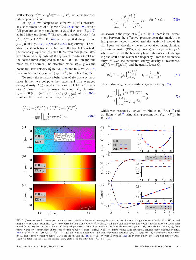
In Fig. 2, we compare an effective (“Eff”) pressure-

acoustics simulation of p1 solving Eqs. (20a) and (25), with a

full pressure-velocity simulation of p1 and v1 from Eq. (17)

as in Muller and Bruus.28 The analytical results (“Ana”) for

pres1 ; vd;res

1y , and vd;res1z in Eq. (69) are also plotted along the line

y ¼ 14

W in Figs. 2(a2), 2(b2), and 2(c2), respectively. The rel-

ative deviation between the full and effective fields outside

the boundary layer are less than 0.1% even though the latter

was obtained using only 5000 degrees of freedom (DoF) on

the coarse mesh compared to the 600 000 DoF on the fine

mesh for the former. The effective model vd1;Eff gives the

boundary-layer velocity vd1 by Eq. (22), and thus by Eq. (18)

the complete velocity v1 ¼ vd1;Eff þ vd

1 (blue dots in Fig. 2).

To study the resonance behaviour of the acoustic reso-

nator further, we compute the space- and time-averaged

energy density h �Edaci stored in the acoustic field for frequen-

cies f close to the resonance frequency fres. Inserting

ky ¼ ðp=WÞð1þ ði=2ÞCblÞ þ ð2p=c0Þðf � fresÞ into Eq. (65),

results in the Lorentzian line-shape for h �Edaci,

�Edac

D E¼ �E

d;kinac

D Eþ �E

d;potac

D E¼ 2 �E

d;potac

D E¼ 2

HW

ð ðXfl

1

2j0 p1p1h i dydz (70a)

�1

p2q0 V0

1y

2

f

fres

� 1

� �2

þ 1

2Cbl

� �2; for f � fres: (70b)

As shown in the graph of h �Edaci in Fig. 3, there is full agree-

ment between the effective pressure-acoustics model, the

full pressure-velocity model, and the analytical model. In

this figure we also show the result obtained using classical

pressure acoustics (CPA, gray curves) with @fp1 ¼ ixq0V01f

where we see that the boundary layer introduces both damp-

ing and shift of the resonance frequency. From the resonance

curve follows the maximum energy density at resonance,

h �Ed;resac i ¼ h �E

dacðfresÞi, and the quality factor Q,

h �Ed;resac i ¼

1

4q0

4V01y

pCbl

!2

; Q ¼ 1

Cbl

¼ H

d: (71)

This is also in agreement with the Q-factor in Eq. (33),

Q ¼2

ð ðXfl

1

4q0jvres

1y j2

dydz

2

ðþW=2

�W=2

1

4dq0jvres

1y j2

dy

¼ H

d; (72)

which was previously derived by Muller and Bruus36 and

by Hahn et al.38 using the approximation Ploss � Pdissvisc in

Eq. (33).

FIG. 2. (Color online) First-order pressure and velocity fields in the vertical rectangular cross section of a long, straight channel of width W ¼ 380 lm and

height H ¼ 160 lm at resonance fres ¼ 1:967 MHz and actuation velocity V01y ¼ 2pfres 0:1 nm. Color plots of the full (upper half) and effective (lower half)

model fields: (a1) the pressure p1 from �1 MPa (dark purple) to 1 MPa (light cyan) and the finite element mesh (gray), (b1) the horizontal velocity v1y from

0 m/s (black) to 0.7 m/s (white), and (c1) the vertical velocity v1z from �1 mm/s (black) to 1 mm/s (white). Line plots [Full, Eff, and Ana¼ analytics from Eq.

(69)] at y0 ¼ 14

W for � 12

H < z < � 12

H þ 7d (light gray dashed lines) of (a2) the relative pressure deviation p1ðy0; zÞ=p1ðy0; 0Þ � 1, (b2) the horizontal veloc-

ity v1y, and (c2) the vertical velocity v1z. Dots are the full velocity (18) v1 ¼ vd1 þ vd

1 with vd1 from Eq. (22) and vd

1 from either “Eff” (dark blue dots) or “Ana”

(light red dots). The insets are the corresponding plots along the entire line � 12

H < z < 12

H.

J. Acoust. Soc. Am. 144 (2), August 2018 Jacob S. Bach and Henrik Bruus 777

B. Second-order streaming solution

For the full model at resonance fres, we solve Eq. (34),

while for the effective model we solve Eq. (52) with the

boundary condition on vd2 obtained by inserting the velocity

fields from Eq. (69) into Eq. (54). At the surfaces z ¼ 6 12

H,

we find to lowest order in �,

vd02y ¼

3

8c0

4V01y

pCbl

!2

sin 2~yð Þ; (73a)

vd02z ¼ 7 k0dð Þ 1

8c0

4V01y

pCbl

!2

1þ 10 cos 2~yð Þ½ �: (73b)

The resulting fields of the two models are shown in Fig. 4.

Again, we have good quantitative agreement between the

two numerical models, now better than 1% or 3k0d, for 9000

DoF and 600 000 DoF, respectively.

Analytically, Eq. (73a) is the usual parallel-direction

boundary condition for the classical Rayleigh streaming,22

while Eq. (73b) is beyond that, being the perpendicular-

direction boundary condition on the streaming, which is a

factor k0d � 3 10�3 smaller than the parallel one. This is

confirmed in Fig. 4(b) showing the streaming velocity close

to z ¼ � 12

H at y ¼ 14

W.

IX. EXAMPLE II: A CURVED OSCILLATING CAVITY

Next, we implement in COMSOL our boundary conditions

(25) and (55) in a system with a curved solid-fluid interface

that oscillates in any direction, as described in Sec. VII. We

consider an ellipsoidal fluid domain (water) of horizontal

major axis W ¼ 380 lm and vertical minor axis H ¼ 160 lm

surrounded by a rectangular solid domain (Pyrex) of width

Wsl ¼ 680 lm and height Hsl ¼ 460 lm, see Fig. 5. We

actuate the solid at its bottom surface using a vertical veloc-

ity amplitude Vactz ¼ d0x sin ðpy=WslÞ with d0 ¼ 0:1 nm and

at the resonance frequency fres ¼ 2:222 MHz, which has

FIG. 3. (Color online) Resonance curves for the rectangular channel. “Ana”

refers to the analytical result from Eq. (70b) and “CPA” refers to simulations

using classical pressure acoustics with the boundary condition @fp1 ¼ ixV01f

at r 2 @X with different choices of bulk damping coefficient C.

FIG. 4. (Color online) Simulated second-order velocity for the rectangular

channel. (a) The full-model v2 (above) and the effictive-model vd2 (below).

(b) Line plots near the center of the dark blue half circle in (a) at y0 ¼ 14

Wfor � 1

2H < z < � 1

2H þ 7d.

FIG. 5. (Color online) Full (left) and effective (right) simulations for a

curved channel with fluid-solid coupling. (a) An elliptic fluid domain with

the acoustic pressure p1 from �0.35 MPa (dark purple) to þ0.35 MPa (light

cyan) and fluid velocity (green arrows, max 0.2 m/s) surrounded by solid

Pyrex with a displacement field usl (dark blue arrows) and displacement

magnitude juslj from 0 nm (black) to 2.7 nm (yellow). To be visible, the dis-

placement (dark blue line and dark blue arrows, max 2.7 nm) is enhanced

104 times, except at the bottom (green line, max 0.1 nm) where it is

enhanced 105 times. (b) Streaming velocity v2 (light green arrows) and mag-

nitude from 0 lm/s (black) to 7:8 lm/s (light yellow). (c) Line plots along

the light ray dashed line in (a) and (b) of p1 normalized by 0.35 MPa and v2

by 7:8 lm/s.

778 J. Acoust. Soc. Am. 144 (2), August 2018 Jacob S. Bach and Henrik Bruus

been determined numerically as in Fig. 3. The linear govern-

ing equations for the displacement field usl of the solid are

those used by Ley and Bruus,48

$ � rsl ¼ �qslx2ð1þ iCslÞu; solid domain; (74a)

�ixusl ¼ Vactz yð Þ ez; actuation at z ¼ � 1

2Hsl; (74b)

nsl � rsl ¼ 0; at solid–air interfaces; (74c)

nsl � rsl ¼ nsl � r1; at solid–fluid interfaces; (74d)

where rsl ¼ qslc2tr½$usl þ ð$uslÞT � þ qslðc2

lo � 2c2trÞð$ � uslÞI

is the stress tensor of the solid with mass density qsl, trans-

verse velocity ctr, longitudinal velocity clo, and damping

coefficient Csl, while nsl is the solid surface normal, and

nsl � r1 ¼ ef � r1 is the fluid stress on the solid, Eq. (26). The

material parameter values are listed in Table I.

We solve numerically Eqs. (20a) and (25) in first order

and Eqs. (52) and (55) in second order. The results are

shown in Fig. 5, where we compare the simulation results

from the full boundary-layer resolved simulation of Eq. (34)

with the effective model. Even for this more complex and

realistic system consisting of an elastic solid with a curved

oscillating interface coupled to a viscous fluid, we obtain

good quantitative agreement between the two numerical

models, better than 1% for 600 000 DoF and 9000 DoF,

respectively.

X. CONCLUSION

We have studied acoustic pressure and streaming in

curved elastic cavities having time-harmonic wall oscilla-

tions in any direction. Our analysis relies on the condition

that both the surface curvature and wall displacement are

sufficiently small as quantified in Eq. (16).

We have developed an extension of the conventional the-

ory of first-order pressure acoustics by including the viscous

effects of the thin viscous boundary layer. Based on this the-

ory, we have also derived a slip-velocity boundary condition

for the steady second-order acoustic streaming, which allows

for efficient computations of the resulting incompressible

Stokes flow.

The core of our theory is the decomposition of the first-

and second-order fields into long- and short-range fields

varying on the large bulk length scale d and the small

boundary-layer length scale d, respectively, see Eqs. (19) and

(35). In the physically relevant limits, this velocity decompo-

sition allows for analytical solutions of the boundary-layer

fields. We emphasize that in contrast to the conventional

second-order matching theory of inner solutions in the bound-

ary layer and outer solutions in the bulk, our long- and short-

range, second-order, time-averaged fields co-exist in the

boundary layer, but the latter die out exponentially beyond the

boundary layer leaving only the former in the bulk.

The main theoretical results of the extended pressure

acoustics in Sec. III are the boundary conditions (25) and

(26) for the pressure p1 and the stress r1 � ef expressed in

terms of the pressure p1 and the velocity V01 of the wall.

These boundary conditions are to be applied to the governing

Helmholtz equation (20a) for p1, and the gradient form (19b)

of the compressional acoustic velocity field vd1. Furthermore,

in Sec. IV, we have used the extended pressure boundary

condition to derive an expression for the acoustic power loss

Ploss, Eq. (32), and the quality factor Q, Eq. (33), for acoustic

resonances in terms of boundary-layer and bulk loss mecha-

nisms. The main results of the streaming theory in Sec. V

are the governing incompressible Stokes equation (52) for

the streaming velocity vd2 and the corresponding extended

boundary condition (55) for the streaming slip velocity vd02 .

In this context, we have developed a compact formalism

based on the IðnÞab -integrals of Eq. (43) to carry out with rela-

tive ease the integrations that lead to the analytical expres-

sion for vd02 . Last, in Sec. VI, we have applied our extended

pressure-acoustics theory to several special cases. We have

shown how it leads to predictions that goes beyond previous

theoretical results in the literature by Lord Rayleigh,22

Nyborg,33 Lee and Wang,34 and Vanneste and B€uhler,35

while it does agree in the appropriate limits with these

results.

The physical interpretation of our extended pressure

acoustics theory may be summarized as follows: The fluid

velocity v1 is the sum of a compressible velocity vd1 and an

incompressible velocity vd1, where the latter dies out beyond

the boundary layer. In general, the tangential component

V01k ¼ vd0

1k þ vd01k of the no-slip condition at the wall induces

a tangential compression of vd1 due to the tangential compres-

sion of vd1 and V0

1. This in turn induces a perpendicular veloc-

ity component vd01f due to the incompressibility of vd

1. To fulfil

the perpendicular no-slip condition V01f ¼ vd0

1f þ vd01f , the per-

pendicular component vd01f of the acoustic velocity must there-

fore match not just the wall velocity V01f, as in classical

pressure acoustics, but the velocity difference V01f � vd0

1f . The

inclusion of vd01f takes into account the power delivered to the

acoustic fields by the tangential wall motion, and the power

lost from the acoustic fields due to tangential fluid motion.

Consequently, by incorporating into the boundary condition

an analytical solution of vd1, our theory leads to the correct

acoustic fields, resonance frequencies, resonance Q-factors,

and acoustic streaming.

In Secs. VII–IX we have demonstrated the implementa-

tion of our extended acoustic pressure theory in numerical

finite-element COMSOL models, and we have presented the

results of two specific models in 2D: a water domain with a

rectangular cross section and a given velocity actuation on

the domain boundary, and a water domain with an elliptic

cross section embedded in a rectangular glass domain that is

actuated on the outer boundary. By restricting our examples

to 2D, we have been able to perform direct numerical simu-

lations of the full boundary-layer-resolved model, and to use

these results for validation of our extended acoustic pressure

and streaming theory. Remarkably, we have found that even

in 2D, our approach makes it possible to simulate acousto-

fluidic systems with a drastic nearly 100-fold reduction in

the necessary degrees of freedom, while achieving the same

quantitative accuracy, typically of order k0d, compared to

direct numerical simulations of the full boundary-layer

resolved model. We have identified three reasons for this

J. Acoust. Soc. Am. 144 (2), August 2018 Jacob S. Bach and Henrik Bruus 779

reduction: (1) Neither our first-order nor our second-order

method involve the fine-mesh resolution of the boundary

layer. (2) Our first-order equations (20a) and (25) requires

only the scalar pressure p1 as an independent variable, while

the vector velocity v1 is subsequently computed from p1, Eq.

(19b). (3) Our second-order equations (52) and (55) avoid

the numerically demanding evaluation in the entire fluid

domain of large terms that nearly cancel, and therefore our

method requires a coarser mesh compared to the full model,

also in the bulk.

The results from the numerical examples in Secs. VIII

and IX show that the extended pressure acoustics theory has

the potential of becoming a versatile and very useful tool in

the field of acoustofluidics. For the fluid-only rectangular

domain in Sec. VIII, we showed how the theory not only

leads to accurate numerical results for the acoustic fields and

streaming, but also allows for analytical solutions, which cor-

rectly predict crucial details related to viscosity of the first-

order acoustic resonance, and which open up for a deeper

analysis of the physical mechanisms that lead to acoustic

streaming. For the coupled fluid-solid system in 2D of an

elliptical water domain embedded in a rectangular glass

block, we showed in Sec. IX an important example of a more

complete and realistic model of an actuated acoustofluidic

system. The extended pressure acoustics theory allowed for

calculations of acoustic fields and streaming with a relative

accuracy lower than 1%. Based on preliminary work in pro-

gress in our group, it appears that the extended pressure

acoustic theory makes 3D simulations feasible within reason-

able memory consumptions for a wide range of microscale

acoustofluidic systems such as fluid-filled cavities and chan-

nels driven by attached piezoelectric crystals as well as drop-

lets in two-phase systems and on vibrating substrates.

Currently, we have neglected thermal dissipation. It would

of course be an obvious and interesting study, to extend the

presented theory to include thermoviscous effects. Previous

studies42,49 on acoustofluidic systems with flat walls oscillating

only in the perpendicular direction, have shown that the acous-

tic streaming is unaffected for channels with a height larger

than 250 d � 100 lm. We thus expect the predictions of this

work to hold for such “high” channels. However, for more flat

channels, a significant reduction of the acoustic streaming is

predicted, for example a reduction factor of 2 for a channel of

height 25d � 10 lm.42 For such “flat” channels, the thermal

boundary-layer must be included in our model to ensure reli-

able predictions. Such an extension of our model seems feasi-

ble, as the thermal boundary-layer width is about 3 times

smaller than the viscous boundary-layer width for water at

2 MHz and 25 �C. Thus the basic idea of a weakly curved, thin

boundary-layer model can be maintained, but of course at the

expense of analytical complications arising from including the

heat transport equation together with temperature dependence

of the material parameters in the presented first- and second-

order perturbation theory.

Although we have developed the extended pressure-

acoustics theory and corresponding streaming theory within

the narrow scope of microscale acoustofluidics, our theories

are of general nature and may likely find a much wider use

in other branches of acoustics.

APPENDIX A: DIFFERENTIAL GEOMETRY

In the following we present the basic differential

geometry used in this work. Because our analysis is carried

out in the limit of weakly curved, thin boundary layers,

defined by �� 1 of Eq. (10) as discussed in Sec. II D,

simplifications arise so that we do not need to unfold the full

notation of differential geometry based on co- and

contravariant derivatives, the metric tensor, and the full

Christoffel symbols.50,51 Instead, we follow the tradition in

the field set by Nyborg33 and by Lee and Wang,34 and use the

vectorial notation based on the unit tangent vectors ei and the

scale factors hi at position r in the thin boundary layer,

ei ¼1

hi@ir; with hi ¼ j@irj for i ¼ n; g; f; (A1a)

ek � ei ¼ dki; orthonormality by construction: (A1b)

It is natural to introduce the scaled derivatives ~@ i and the

curvilinear quantities Tkji and Hk,

~@ i ¼ h�1i @i; so that ei ¼ ~@ ir; (A2a)

Tkji ¼ ð~@ kejÞ � ei; for k; j; i ¼ n; g; f; (A2b)

Hk ¼ Tiki; sum over repeated index i: (A2c)

Tkji is related to, but not identical with, the celebrated

Christoffel symbols of differential geometry. The following

relations for Tkji are useful in the analysis:

Tkji ¼ Tjki; for i 6¼ j; (A3a)

Tknn ¼ Tkgg ¼ Tkff ¼ 0; (A3b)

Tfji ¼ 0: (A3c)

Equation (A3a) follows from Tkji ¼ ð1=hkÞ@kðð1=hjÞ@jrÞ � ei

¼ ð@k@jr=hkhjÞ � ei � ð@khj=hkhjÞej � ei, which is symmetric

in k and j as the last term is zero for j 6¼ i, Eq. (A3b) is

proven by observing Tknn ¼ ð~@ kenÞ � en ¼ 12

~@ kðen � enÞ ¼ 0

as en � en ¼ 1, and Eq. (A3c) arises because f is defined as

the normal direction, and as a consequence Tkji is only non-

zero for the tangential derivatives Tnji and Tgji, and

Hk ¼ Tnkn þ Tgkg. It is in this sense that the surface length

scale is set by R minfT�1kji ;H�1

k g as stated in Sec. II E.

From now on, we use the index notation, where, as in

Eq. (A2c), a repeated index implies a summation. In

curvilinear coordinates, the $ operator and vector fields are

written as

$ ¼ ei~@ i; A ¼ Ai ei; (A4)

and from this all other differential operators are calculated.

The first example is the Laplacian of a scalar,

r2g ¼ $ � $g ¼ ðej~@ jÞ � ei

~@ ig

¼ ej � ei~@ j þ ej � ð~@ jeiÞ

h i~@ ig

¼ ð~@ i þ TjijÞ~@ ig ¼ ð~@ i~@ i þHi

~@ iÞg: (A5)

780 J. Acoust. Soc. Am. 144 (2), August 2018 Jacob S. Bach and Henrik Bruus

The divergence of a vector field A takes the form

$ � A ¼ ei � ~@ iðAkekÞ ¼ ð~@ iAkÞek þ Ak~@ iek

h i� ei

¼ ð~@ iAkÞdik þ AkTiki ¼ ð~@ k þHkÞAk; (A6)

while the gradient of a vector field B is

$B ¼ ek~@ kðBjejÞ ¼ ek ð~@ kBiÞei þ Bj

~@ kej

h i¼ ekð~@ kBi þ TkjiBjÞei: (A7)

From this follows the advective derivative ðA � $ÞB of a

vector B with respect to a vector A,

ðA � $ÞB ¼ Akð~@ kBi þ TkjiBjÞei; (A8)

and the Laplacian of a vector B,

r2B ¼ $ � $B ¼ en~@n ekð~@ kBi þ TkjiBjÞei

h i¼ Hkð~@ kBi þ TkjiBjÞei

þ ~@ k~@ kBi þ Bj

~@ kTkji þ Tkji~@ kBj

h iei

þ ð~@ kBi þ TkjiBjÞTkimem: (A9)

In the analysis of fields in the weakly curved, thin

boundary layer, it is useful to decompose a given vector A

into parallel and perpendicular components,

A ¼ Ak þ Af ef; (A10a)

Ak ¼ An en þ Ag eg ¼ Aa ea; (A10b)

where here and in the following, repeated Greek index aonly sums over the tangential indices n and g. Likewise, the

parallel components of the $ operator (A4), the divergence

(A6), and the advective derivative (A8) are

$k ¼ ea~@a; (A11a)

$k � Ak ¼ ð~@a þHaÞAa; (A11b)

ðA � $kÞB ¼ Aað~@aBi þ TajiBjÞei; (A11c)

For the short-ranged boundary-layer vector field

Ad ¼ Ad0 ðn; gÞ adðfÞ introduced in Eq. (14), and the

analogous scalar field gd ¼ gd0ðn; gÞ adðfÞ, the derivative

expressions simplifies in the weakly curved thin boundary-

layer limit �� 1. The reason is that terms containing

surface-derivative quantities $k, Tkji, and Hk, all of size d�1,

are a factor of � smaller than terms with the perpendicular

derivative ~@ f ¼ @f, which picks up a factor of d�1 due to the

factor adðfÞ that decays on the length scale d.

For r2gd in Eq. (A5), the first term ~@ i~@ ig

d ¼ @2f gd

d�2gd is ��1 larger than the second term Hi~@ ig

d

R�1d�1gd, so thatr2gd � @2f gd as stated in Eq. (15a).

Similarly, for r2Ad in Eq. (A9), the only term that does

not contain at least one factor Hk or Tkji is

ð~@ k~@ kAd

i Þ ei � ð@2f Ad

i Þ ei ¼ @2f Ad as stated in Eq. (15b).

Finally, for Eq. (A6), $ � Ad ¼ $k � Adk þ ð~@ f þHfÞAd

f� $k � Ad

k þ @fAdf as stated in Eq. (15c).

APPENDIX B: ACOUSTIC POWER BALANCE

The time averages hEkinac i; hEpot

ac i, and hEaci of the

kinetic, the potential, and the total acoustic energy density,

respectively, are given by

Ekinac

� �¼ 1

2q0 v1 � v1h i; (B1a)

Epotac

� �¼ 1

2j0 p1p1h i; (B1b)

hEaci ¼ hEkinac i þ hEpot

ac i: (B1c)

Using Gauss’s theorem and q0@tv1 ¼ $ � r1, the time-

averaged total power delivered by the surrounding wall is

written as the sum of the time-averaged rate of change of the

acoustic energy and total power dissipated into heat,þ@XhV0

1 � r1i � n dA

¼ð

X$ � hv1 � r1i dV (B2a)

¼ð

Xhv1 � ð$ � r1Þi þ hð$v1Þ : r1i½ �dV (B2b)

¼ð

Xh@tEaci þ hð$v1Þ : s1i½ �dV: (B2c)

Solving for the time-averaged change in acoustic energyÐXh@tEacidV in Eq. (B2c) givesð

Xh@tEacidV

¼þ@XhV0

1 �r1i �ndA�ð

Xhð$v1Þ : s1idV (B3a)

¼þ@XhV0

1ð�p1Þi � n dAþð

Xhv1 � ð$ � s1Þi dV;

(B3b)

where Gauss’s theorem transformsÐ@XhV

01 � s1i � n dA into a

volume integral, and n ¼ �ef is the normal vector of the

fluid domain X. We may interpret the last term in Eq. (B3b)

as the rate of change of stored energy due to the viscosity-

induced power hPvisci,

hPvisci ¼ hPdissvisci þ hPwall

visc i: (B4)

Here, hPdissvisci is the viscous power dissipation into heat and

hPwallvisc i is the power from the viscous part of the work

performed by the wall on the fluid,

hPvisci ¼ð

Xhv1 � ð$ � s1ÞidV; (B5a)

J. Acoust. Soc. Am. 144 (2), August 2018 Jacob S. Bach and Henrik Bruus 781

hPdissvisci ¼ �

ðXhð$ � v1Þ : s1i dV; (B5b)

hPwallvisc i ¼

þ@Xhv1 � s1i � n dA: (B5c)

Using Eqs. (18) and (19) we evaluate hPvisci,

hPvisci ¼ð

Xhv1 � ð$ � s1Þi dV (B6a)

¼ð

Xhv1 � ðiC$p1 � ixq0v

d1Þi dV (B6b)

¼ð

X�Cxq0

2jvd

1j2 þ @tE

kin;dac

� �� �dV

�þ@Xhp1v

d01 i � n dA; (B6c)

where we used Eq. (19) and Gauss’s theorem. Inserting Eq.

(B6c) into Eq. (B3b) leads to Eq. (30). Comparing with Eq.

(32), we can relate hPlossi ¼ hPdlossi and hPvisci,

Plossh i¼ Pvisch i�þ@X

p1

i

ks

$k �V01k

� �� �� ndA (B7a)

¼ Pdissvisc

� �þ Pwall

visc

� ��þ@X

p1

i

ks

$k �V01k

� �� ��ndA:

(B7b)

Note that hPlossi is not in general the same as the power

hPdissvisci dissipated into heat. These might, however, be

approximately equal if the powerþ@X� hp1V0

1i � n dA

delivered by the pressure is approximately balanced by

dissipation hPdissvisci. This happens, if

þ@X� hp1V0

1i � n dA

is much larger than hPwallvisc i and

þ@X

p1

i

ks

$k � V01k

� �� �� n dA;

which is usually satisfied.

APPENDIX C: COMPARISON WITH PREVIOUSRESULTS IN THE LITERATURE

1. Comparison with Lee and Wang (1989)

In the following we rewrite the n-component vd02n of the

streaming velocity in Eq. (58a) using the notation of Lee

and Wang34 to compare it directly with uL given in their

Eq. (19)LW. First, we take the complex conjugate of the

argument of the real value, set b ¼ n, and write explicitly

the sum over the repeated index a ¼ n; g,

vd02n¼�

1

4xRe vd0

1n~@nv

d0�1n

þvd0

1nvd0�1g Tngn

nþvd0

1g~@gv

d0�1n

þvd0

1gvd0�1g Tggnþ 2þ ið Þ$ � vd

1

� 2þ3ið Þ@fv

d1f� 2� ið ÞHfV

0�1f �vd�

1n

�2iV0�1f @fv

d1nþvd0

1nTnfnþvd01gTgfn

o: (C1)

This expression is rewritten using the notation of Lee and

Wang, vd1¼ua0; ðvd0

1n;vd01g;v

d01fÞ¼ðua0;va0;wa0Þ; ðn;g;fÞ

¼ðx;y;zÞ; Hf¼H;ð~@n;~@g;~@ fÞ¼ð@x1; @x2

;@x3Þ;Tkji¼TLW

ijk , and

V01f¼wa0þOð�Þ,

vd02n¼�

1

4xRe ua0 @x1

u�a0þv�a0TLW121

��þva0 @x2

u�a0þv�a0TLW122 þu�a0 2þ ið Þ$ � ua0½

� 2þ 3ið Þ@zwa0� 2� ið ÞHwa0���2iw�a0 @zua0þua0TLW

131 þva0TLW132

� �g

¼� 1

4xRe qxþu�a0 2þ ið Þ$ � ua0½�

� 2þ3ið Þ@zwa0� 2� ið ÞHwa0��2iw�a0 @zua0þua0TLW

131 þva0TLW132

� �g

¼uLþ1

2xRe iw�a0 @zua0þua0TLW

131 þva0TLW132

� �� �: (C2)

Here, we have used the definition of qx in Eq. (3)LW and the

result in Eq. (19)LW for the x-component uL of the streaming

velocity just outside the boundary layer.

Similarly, we obtain for the g-component vd02g in Eq. (58a),

vd02g ¼ vL þ

1

2xRe iw�a0 @zva0 þ ua0TLW

231 þ va0TLW232

� �� �;

(C3)

where we have used the definition in Eq. (4)LW for qy and

the result in Eq. (20)LW for the y-component vL of the

streaming velocity. The comparison obtained in Eqs. (C2)

and (C3) is discussed in Sec. VI A.

2. Comparison with Vanneste and B€uhler (2011)

In the following we rewrite the n-component vd02n of the

Eulerian streaming velocity in Eq. (59b) using the notation of

Vanneste and B€uhler35 to compare it directly with the

Lagrangian streaming velocity �uLslip given in their Eq. (4.10)VB.

First, given the flat wall, ðn; g; fÞ ¼ ðx; y; zÞ and for all i, j, kwe have hi¼ 1, Hi ¼ 0, and Tijk¼ 0. Then, we identify our

first-order velocity fields with theirs: From Eqs. (2.6)VB and

(3.1)VB follows vd1 ¼ 2$/, and from Eqs. (3.9)VB and

(3.10)VB we read that vd01k ¼ �2Uex �2Vey. Next, we relate

our steady Eulerian second-order velocity vd2 with their

Lagrangian mean flow �uLslip Eq. (4.10)VB. Using ReZ ¼ 1

2Z

þc:c: ¼ 12

Z� þ c:c:, we obtain

782 J. Acoust. Soc. Am. 144 (2), August 2018 Jacob S. Bach and Henrik Bruus

vd02n ¼�

1

4xRe 1� 2ið Þvd0�

1a @avd01n� 4ivd0�

1a @avd01nþ 2þ ið Þ@av

d0�1a þ 2i @av

d0�1a �@fv

d�1f

h ivd0

1n� 2ivd�1k@kv

d1n

n o¼� 1

2x1þ 2ið ÞU@xU

� þ 1þ 2ið ÞV@yU� þ 4iU

�@2

x /þ 4iV�@x@y/

nþ 2þ ið Þ@xU

� þ 2þ ið Þ@yV� þ 2i @2

x /þ @2y /� @2

z / h i

U�oþ c:c:� 1

xivd

1 �$vd1

� �¼� 1

2x3 1þ ið ÞU@xU

� þ 1 þ 2ið ÞV@yU� þ 2 þ ið ÞU@yV

�n o

� i

x2@x@y/V

� þ @2x /þ @2

y /� @2z /

U�n oþ c:c:� uS

¼ uLslip� uS ¼ uE

slip: (C4)

Here, we have used that the Lagrangian velocity uLslip, calcu-

lated by Vanneste and B€uhler in their Eq. (4.10)VB, is related

to the Eulerian velocity uEslip through the Stokes drift velocity

uS ¼ ð1=xÞhivd1 � $vd

1i of Eq. (34c).

Similarly, for the y component vd02g of the streaming,

vd02g ¼ vL

slip � vS ¼ vEslip: (C5)

The comparison obtained in Eqs. (C4) and (C5) is discussed

in Sec. VI B.

1H. Bruus, J. Dual, J. Hawkes, M. Hill, T. Laurell, J. Nilsson, S. Radel, S.

Sadhal, and M. Wiklund, “Forthcoming lab on a chip tutorial series on

acoustofluidics: Acoustofluidics-exploiting ultrasonic standing wave

forces and acoustic streaming in microfluidic systems for cell and particle

manipulation,” Lab Chip 11(21), 3579–3580 (2011).2T. Laurell and A. Lenshof, Microscale Acoustofluidics (Royal Society of

Chemistry, Cambridge, 2015).3P. Thevoz, J. D. Adams, H. Shea, H. Bruus, and H. T. Soh,

“Acoustophoretic synchronization of mammalian cells in microchannels,”

Anal. Chem. 82(7), 3094–3098 (2010).4P. Augustsson, C. Magnusson, M. Nordin, H. Lilja, and T. Laurell,

“Microfluidic, label-free enrichment of prostate cancer cells in blood

based on acoustophoresis,” Anal. Chem. 84(18), 7954–7962 (2012).5P. Augustsson, J. T. Karlsen, H.-W. Su, H. Bruus, and J. Voldman, “Iso-

acoustic focusing of cells for size-insensitive acousto-mechanical

phenotyping,” Nat. Commun. 7, 11556 (2016).6X. Ding, S.-C. S. Lin, B. Kiraly, H. Yue, S. Li, I.-K. Chiang, J. Shi, S. J.

Benkovic, and T. J. Huang, “On-chip manipulation of single micropar-

ticles, cells, and organisms using surface acoustic waves,” Proc. Natl.

Acad. Sci. U.S.A. 109(28), 11105–11109 (2012).7D. J. Collins, B. Morahan, J. Garcia-Bustos, C. Doerig, M. Plebanski, and

A. Neild, “Two-dimensional single-cell patterning with one cell per well

driven by surface acoustic waves,” Nat. Commun. 6, 8686 (2015).8B. Hammarstr€om, M. Evander, H. Barbeau, M. Bruzelius, J. Larsson, T.

Laurell, and J. Nillsson, “Non-contact acoustic cell trapping in disposable

glass capillaries,” Lab Chip 10(17), 2251–2257 (2010).9B. Hammarstr€om, T. Laurell, and J. Nilsson, “Seed particle enabled acous-

tic trapping of bacteria and nanoparticles in continuous flow systems,”

Lab Chip 12, 4296–4304 (2012).10B. Hammarstr€om, M. Evander, J. Wahlstr€om, and J. Nilsson, “Frequency

tracking in acoustic trapping for improved performance stability and sys-

tem surveillance,” Lab Chip 14, 1005–1013 (2014).11B. W. Drinkwater, “Dynamic-field devices for the ultrasonic manipulation

of microparticles,” Lab Chip 16, 2360–2375 (2016).12D. J. Collins, C. Devendran, Z. Ma, J. W. Ng, A. Neild, and Y. Ai,

“Acoustic tweezers via sub-time-of-flight regime surface acoustic waves,”

Sci. Adv. 2(7), e1600089 (2016).13H. G. Lim, Y. Li, M.-Y. Lin, C. Yoon, C. Lee, H. Jung, R. H. Chow, and

K. K. Shung, “Calibration of trapping force on cell-size objects from

ultrahigh-frequency single-beam acoustic tweezer,” IEEE Trans. Ultrason.

Ferroelectr. Freq. Control 63(11), 1988–1995 (2016).14D. Baresch, J.-L. Thomas, and R. Marchiano, “Observation of a single-

beam gradient force acoustical trap for elastic particles: Acoustical

tweezers,” Phys. Rev. Lett. 116, 024301 (2016).

15L. V. King, “On the acoustic radiation pressure on spheres,” Proc. R. Soc.

London, Ser. A 147(861), 212–240 (1934).16K. Yosioka and Y. Kawasima, “Acoustic radiation pressure on a com-

pressible sphere,” Acustica 5, 167–173 (1955).17A. A. Doinikov, “Acoustic radiation force on a spherical particle in a vis-

cous heat-conducting fluid. I. General formula,” J. Acoust. Soc. Am.

101(2), 713–721 (1997).18A. A. Doinikov, “Acoustic radiation force on a spherical particle in a vis-

cous heat-conducting fluid. II. Force on a rigid sphere,” J. Acoust. Soc.

Am. 101(2), 722–730 (1997).19A. A. Doinikov, “Acoustic radiation force on a spherical particle in a vis-

cous heat-conducting fluid. III. Force on a liquid drop,” J. Acoust. Soc.

Am. 101(2), 731–740 (1997).20M. Settnes and H. Bruus, “Forces acting on a small particle in an acousti-

cal field in a viscous fluid,” Phys. Rev. E 85, 016327 (2012).21J. T. Karlsen and H. Bruus, “Forces acting on a small particle in an acous-

tical field in a thermoviscous fluid,” Phys. Rev. E 92, 043010 (2015).22Lord Rayleigh, “On the circulation of air observed in Kundt’s tubes, and

on some allied acoustical problems,” Philos. Trans. R. Soc. London 175,

1–21 (1884).23H. Schlichting, “Berechnung ebener periodischer grenzeschichtstr€omungen,”

Phys. Z. 33, 327–335 (1932).24M. Wiklund, R. Green, and M. Ohlin, “Acoustofluidics 14: Applications

of acoustic streaming in microfluidic devices,” Lab Chip 12, 2438–2451

(2012).25P. B. Muller, M. Rossi, A. G. Marin, R. Barnkob, P. Augustsson, T.

Laurell, C. J. K€ahler, and H. Bruus, “Ultrasound-induced acoustophoretic

motion of microparticles in three dimensions,” Phys. Rev. E 88(2),

023006 (2013).26J. Lei, P. Glynne-Jones, and M. Hill, “Modal Rayleigh-like streaming in

layered acoustofluidic devices,” Phys. Fluids 28, 012004 (2016).27A. Riaud, M. Baudoin, O. Bou Matar, L. Becerra, and J.-L. Thomas,

“Selective manipulation of microscopic particles with precursor swirling

Rayleigh waves,” Phys. Rev. Appl. 7, 024007 (2017).28P. B. Muller, R. Barnkob, M. J. H. Jensen, and H. Bruus, “A numerical

study of microparticle acoustophoresis driven by acoustic radiation

forces and streaming-induced drag forces,” Lab Chip 12, 4617–4627

(2012).29R. Barnkob, P. Augustsson, T. Laurell, and H. Bruus, “Acoustic radiation-

and streaming-induced microparticle velocities determined by microparti-

cle image velocimetry in an ultrasound symmetry plane,” Phys. Rev. E 86,

056307 (2012).30M. Antfolk, P. B. Muller, P. Augustsson, H. Bruus, and T. Laurell,

“Focusing of sub-micrometer particles and bacteria enabled by two-

dimensional acoustophoresis,” Lab Chip 14, 2791–2799 (2014).31Z. Mao, P. Li, M. Wu, H. Bachman, N. Mesyngier, X. Guo, S. Liu, F.

Costanzo, and T. J. Huang, “Enriching nanoparticles via acoustofluidics,”

ACS Nano 11(1), 603–612 (2017).32M. Wu, Z. Mao, K. Chen, H. Bachman, Y. Chen, J. Rufo, L. Ren, P. Li, L.

Wang, and T. J. Huang, “Acoustic separation of nanoparticles in continu-

ous flow,” Adv. Funct. Mater. 27(14), 1606039 (2017).33W. L. Nyborg, “Acoustic streaming near a boundary,” J. Acoust. Soc. Am.

30(4), 329–339 (1958).34C. Lee and T. Wang, “Near-boundary streaming around a small sphere

due to 2 orthogonal standing waves,” J. Acoust. Soc. Am. 85(3),

1081–1088 (1989).35J. Vanneste and O. B€uhler, “Streaming by leaky surface acoustic waves,”

Proc. R. Soc. London, Ser. A 467(2130), 1779–1800 (2011).

J. Acoust. Soc. Am. 144 (2), August 2018 Jacob S. Bach and Henrik Bruus 783

36P. B. Muller and H. Bruus, “Theoretical study of time-dependent, ultra-

sound-induced acoustic streaming in microchannels,” Phys. Rev. E 92,

063018 (2015).37C. E. Bradley, “Acoustic streaming field structure: The influence of the

radiator,” J. Acoust. Soc. Am. 100(3), 1399–1408 (1996).38P. Hahn and J. Dual, “A numerically efficient damping model for acoustic

resonances in microfluidic cavities,” Phys. Fluids 27, 062005 (2015).39A. Riaud, M. Baudoin, O. Bou Matar, J.-L. Thomas, and P. Brunet, “On

the influence of viscosity and caustics on acoustic streaming in sessile

droplets: An experimental and a numerical study with a cost-effective

method,” J. Fluid Mech. 821, 384–420 (2017).40C. Eckart, “Vortices and streams caused by sound waves,” Phys. Rev. 73,

68–76 (1948).41COMSOL Multiphysics 5.3a (2017), www.comsol.com (Last viewed 3

August 2018).42P. B. Muller and H. Bruus, “Numerical study of thermoviscous effects in

ultrasound-induced acoustic streaming in microchannels,” Phys. Rev. E

90(4), 043016 (2014).43M. W. H. Ley and H. Bruus, “Continuum modeling of hydrodynamic

particle-particle interactions in microfluidic high-concentration sus-

pensions,” Lab Chip 16(7), 1178–1188 (2016).

44CORNING, Houghton Park C-8, Corning, NY 14831, USA, Glass SiliconConstraint Substrates, http://www.valleydesign.com/Datasheets/

Corning%20Pyrex%207740.pdf (Last viewed April 18, 2018).45R. Barnkob, P. Augustsson, T. Laurell, and H. Bruus, “Measuring the local

pressure amplitude in microchannel acoustophoresis,” Lab Chip 10(5),

563–570 (2010).46P. Augustsson, R. Barnkob, S. T. Wereley, H. Bruus, and T. Laurell,

“Automated and temperature-controlled micro-PIV measurements

enabling long-term-stable microchannel acoustophoresis character-

ization,” Lab Chip 11(24), 4152–4164 (2011).47R. Barnkob, I. Iranmanesh, M. Wiklund, and H. Bruus, “Measuring acous-

tic energy density in microchannel acoustophoresis using a simple and

rapid light-intensity method,” Lab Chip 12, 2337–2344 (2012).48M. W. H. Ley and H. Bruus, “Three-dimensional numerical modeling of

acoustic trapping in glass capillaries,” Phys. Rev. Appl. 8, 024020 (2017).49A. Y. Rednikov and S. S. Sadhal, “Acoustic/steady streaming from a

motionless boundary and related phenomena: Generalized treatment of the

inner streaming and examples,” J. Fluid. Mech. 667, 426–462 (2011).50E. Kreyszig, Differential Geometry (Dover Publications, New York, 1991).51L. D. Landau and E. M. Lifshitz, The Classical Theory of Fields, 4th ed.

(Butterworth-Heinemann, Oxford, 1980), Vol. 4.

784 J. Acoust. Soc. Am. 144 (2), August 2018 Jacob S. Bach and Henrik Bruus