forces acting on microparticles in acousto uidic...
TRANSCRIPT

Forces Acting on Microparticles in
Acoustofluidic Systems
Bachelor Thesis
Lasse Mejling Andersen, s062087
Anders Nysteen, s062121
Mikkel Settnes, s052944
DTU Nanotech
Technical University of Denmark
Supervisor: Henrik Bruus
Date: June 18, 2009

Abstract i
Abstract
Handling microparticles in lab-on-a-chip systems can be very difficult using traditionalmechanical approaches. Acoustofluidics presents a method to manipulate the particles byattaching a piezo-actuator to the chip, where the vibrations cause the particles to movetowards the (anti-)nodes of the applied pressure field.
In this thesis we describe the governing equations for acoustofluidics and resonance ef-fects, and with the non-linear Navier–Stokes equation as a starting point we use a second-order perturbation scheme to derive the time-independent acoustic pressure force on spher-ical, compressible particles in a standing wave. We focus on deriving the acoustic pressureforce in details following a classical article by Gor’kov, [14], and look at its applications inthree designs proposed by different research groups: Separation of lipid particles from redblood cells, separation of red and white blood cells, and finally how to separate large lipidparticles from raw milk. We found that it theoretically was possible to create microchannelsystems where these separations were possible using the pressure force. Furthermore wediscussed how to optimize the designs to achieve good separation and/or high throughputof the test sample.
An important point in the optimization was to use channels with varying widths to getdifferent patterns of standing waves in the channel, i.e. using the first part of the channelto focus the particles in one beam and next leading them into a channel with a differentwidth where the separation is taking place.
Finally we discuss some of the neglected effects in our model. When considering longi-tudinal modes in standard separation setups, the particle trajectories can be approximatedvery well by the trajectories in a system neglecting longitudinal modes with half the acous-tic energy density. For separation of smaller particles with radii < 1 µm, the acousticstreaming is shown to have a greater importance in the description of the particle move-ment, and for larger particles with radii > 20 µm the interparticle interaction described bythe secondary Bjerknes force must be taken into consideration.

ii Abstract

Resumé iii
Resumé
Håndtering af mikropartikler i lab-on-a-chip-systemer kan være meget besværligt ved hjælpaf traditionelle mekaniske fremgangsmåder. Akustofluidik tilbyder en metode til at ma-nipulere partikler på ved at fastgøre en piezo-aktuator på chippen, så vibrationerne fårpartiklerne til at bevæge sig imod (anti-)knudepunkter for den påtrykte trykbølge.
I denne afhandling beskriver vi de grundlæggende ligninger for akustofluidik og reso-nanseffekter, og med udgangspunkt i den ikke-lineære Navier–Stokes-ligning benytter vianden-ordens perturbation til at udlede den tidsuafhængige akustiske trykkraft på sfæriske,kompressible partikler i en stående bølge. Vi vil lægge vægt på at udlede den akustisketrykkraft i detaljer med udgangspunkt i en klassisk artikel af Gor’kov, [14], og kigge på densanvendelsesmuligheder i tre forskellige designs foreslået af forskellige forskningsgrupper:Separation af fedtpartikler fra røde blodlegemer, separation af røde og hvide blodlegemerog til sidst hvordan store fedtpartikler kan separeres fra råmælk. Vi fandt, at det teoretiskset var muligt at lave mikrokanalsystemer, hvor disse separationer var mulige ved hjælp aftrykkraften. Endvidere diskuterede vi, hvorledes designene skulle optimeres for at få godseparation og/eller højt gennemløb af prøvematerialet.
En vigtig pointe med hensyn til optimeringen var at benytte kanaler med varierendebredde for at få forskellige stående bølger i kanalen, det vil sige at udnytte den første delaf kanalen til at fokusere partiklerne i en stråle og dernæst lede dem ind i en kanal med enanden bredde, hvor selve separationen finder sted.
Til sidst diskuterer vi nogen af de negligerede effekter i vores model. Når vi be-tragter longitudinale modes i standardkanaler for partikelseparation, kan partikelbanernetilnærmes meget godt med partikelbanerne i et system, hvor longitudinale modes negliceres,men hvor den akustiske energi er halvt så stor. For separation af mindre partikler medradius < 1 µm er det vist, at den akustiske strømning får større betydning for beskrivelsenaf partikelbevægelsen, og for større partikler med radius > 25 µm, må der tages hensyn tilpåvirkningen mellem partiklerne beskrevet ved den sekundære Bjerknes-kraft.

iv Resumé

Preface v
Preface
This bachelor-thesis treats the theoretical background of acoustofluidics as well as looksat its applications. It is written as part of the B.Sc. Eng. education at the TechnicalUniversity of Denmark.
The thesis corresponds to 15 ECTS points of work for each student, corresponding to aquarter of a year for each, and was prepared at the Theoretical Microfluidics (TMF) groupat DTU Nanotech in the spring semester 2009.
We would like to thank the group of Prof. Thomas Laurell at the University of Lundfor giving us valuable insights in the practical aspects of acoustofluidics. Furthermore wewould also like to thank Jacob Riis Folkenberg at Foss for giving us ideas on the separationof lipids in milk.
At DTU Nanotech we would especially like to thank M.Sc. student Rune Barnkobfor his tireless help and limitless patience when we had questions or problems regardingMatlab or standing waves in the fluid. We would also like to thank him for sharing hisuseful experimental results with us, which helped us validate our theoretical model. Lastbut not least our very deepest gratitude goes to our supervisor Prof. Henrik Bruus for hisdeep understanding of fluidics and the math involved. He has also been a good guidelineon how to improve the writing and presentation of this thesis.
The content of the thesis corresponds to 98 written pages when not counting the blankpages. Due to demands from the Danish Ministry of Education, we are required to writewho is responsible for which parts of the thesis. Let p = {n ∈ N | n ≤ plast} where plast isthe last page of the thesis. Using this we have made the following division of pages p
pAnders = {p | p ≡ 0 (mod 3)} , (1)
pLasse = {p | p ≡ 1 (mod 3)} , (2)
pMikkel = {p | p ≡ 2 (mod 3)} . (3)
It should be understood such that the person responsible for the pages above wrote theinitial draft while the two others reviewed it. Chapters 1 and 13 were written together.
Lasse Mejling Andersen, Anders Nysteen, and Mikkel SettnesDTU Nanotech – Department of Micro and Nanotechnology
Technical University of DenmarkJune 18, 2009

vi Preface

Contents vii
Contents
List of Figures xii
List of Tables xiii
List of Symbols xv
1 Introduction 1
1.1 Background for Lab-on-a-chip Systems . . . . . . . . . . . . . . . . . . . . . 1
1.2 Acoustophoresis . . . . . . . . . . . . . . . . . . . . . . . . . . . . . . . . . . 2
1.3 Experimental Motivation . . . . . . . . . . . . . . . . . . . . . . . . . . . . . 2
1.4 Outline of the Thesis . . . . . . . . . . . . . . . . . . . . . . . . . . . . . . . 3
I Theory 7
2 Governing Equations and Perturbation Theory 9
2.1 Momentum and Density . . . . . . . . . . . . . . . . . . . . . . . . . . . . . 9
2.2 Perturbation Theory . . . . . . . . . . . . . . . . . . . . . . . . . . . . . . . 10
2.2.1 Zeroth-order Perturbation Equations . . . . . . . . . . . . . . . . . . 11
2.2.2 First-order Perturbation Equations . . . . . . . . . . . . . . . . . . . 11
2.2.3 Second-order Perturbation Equations . . . . . . . . . . . . . . . . . . 11
3 Acoustic Waves in Fluids 13
3.1 Inviscid First-order Acoustic Field . . . . . . . . . . . . . . . . . . . . . . . 13
3.1.1 The Wave Equation for Irrotational First-order Inviscid Velocity Per-turbation . . . . . . . . . . . . . . . . . . . . . . . . . . . . . . . . . 13
3.1.2 Inviscid First-order Harmonic Time-dependent Waves . . . . . . . . 14
3.2 First-order Viscid Acoustic Field . . . . . . . . . . . . . . . . . . . . . . . . 14
3.2.1 Viscid Harmonic Time-dependent Waves in First-order . . . . . . . . 15
3.3 Condition for Incompressible Behavior . . . . . . . . . . . . . . . . . . . . . 17
3.4 Inviscid Second-order Acoustic Field . . . . . . . . . . . . . . . . . . . . . . 19
3.5 Calculation of Time Average . . . . . . . . . . . . . . . . . . . . . . . . . . . 20

viii Contents
4 Resonance in First-order Theory 21
4.1 Acoustic Resonance in a Single-domain System . . . . . . . . . . . . . . . . 21
4.1.1 Considering the Perturbation Parameter and the First-order Velocity 23
4.1.2 Energy in the Resonator . . . . . . . . . . . . . . . . . . . . . . . . . 24
5 Forces on Microparticles 27
5.1 The Potential Flow . . . . . . . . . . . . . . . . . . . . . . . . . . . . . . . . 27
5.2 The Average Force For Second-order Perturbation . . . . . . . . . . . . . . . 28
5.2.1 Calculation of the Velocity Potential . . . . . . . . . . . . . . . . . . 29
5.3 Forces Acting on a Particle in a Plane Running Wave . . . . . . . . . . . . . 34
5.4 Forces Acting on a Particle in an Arbitrary Wave . . . . . . . . . . . . . . . 37
5.5 Pressure Force on a Single Particle in a Standing Wave . . . . . . . . . . . . 41
5.6 Visualizing the Pressure Force and the Idea Behind Particle Separation . . . 42
5.7 Considering the Pressure Force in 2D . . . . . . . . . . . . . . . . . . . . . . 43
II Discussion of Applications in the Single-Particle Approach 45
6 Analytic Solution for Single-Particle 47
6.1 Travel Time . . . . . . . . . . . . . . . . . . . . . . . . . . . . . . . . . . . . 47
6.2 Distance Traveled in Longitudinal Direction . . . . . . . . . . . . . . . . . . 49
6.3 Experimental Verification of Theory . . . . . . . . . . . . . . . . . . . . . . 51
7 Introduction to Separating Systems 53
7.1 The Channel Setup . . . . . . . . . . . . . . . . . . . . . . . . . . . . . . . . 53
7.2 The Simulations . . . . . . . . . . . . . . . . . . . . . . . . . . . . . . . . . 55
8 Separation of Red Blood Cells and Lipid Particles 57
8.1 Lipid Size . . . . . . . . . . . . . . . . . . . . . . . . . . . . . . . . . . . . . 58
8.2 Finding the Flow Rate . . . . . . . . . . . . . . . . . . . . . . . . . . . . . . 59
8.3 One-inlet Channel . . . . . . . . . . . . . . . . . . . . . . . . . . . . . . . . 59
8.4 Three-inlet Channel . . . . . . . . . . . . . . . . . . . . . . . . . . . . . . . 61
8.5 Five-inlet Channel . . . . . . . . . . . . . . . . . . . . . . . . . . . . . . . . 61
8.6 A 3/2 λ-harmonic System . . . . . . . . . . . . . . . . . . . . . . . . . . . . 61
8.7 Summary . . . . . . . . . . . . . . . . . . . . . . . . . . . . . . . . . . . . . 63
9 Separation of Red and White Blood Cells 65
9.1 Separation by Different Channel Designs . . . . . . . . . . . . . . . . . . . . 65
9.1.1 Separation in BWB-system, Varying Inner Edge of Blood Inlet . . . 67
9.1.2 Separation in WBWBW-system, With Variable Width of Blood Inlet 69
9.1.3 Separation in WBWBW-system, With Variable Position of Blood Inlet 70
9.2 Concentration of White Blood Cells . . . . . . . . . . . . . . . . . . . . . . 71
9.3 Changing the Transport Medium . . . . . . . . . . . . . . . . . . . . . . . . 72
9.4 Summary . . . . . . . . . . . . . . . . . . . . . . . . . . . . . . . . . . . . . 74

Contents ix
10 Separation of Lipid Particles in Milk 75
10.1 Design Considerations . . . . . . . . . . . . . . . . . . . . . . . . . . . . . . 75
10.2 Analytical View on the Sorting . . . . . . . . . . . . . . . . . . . . . . . . . 78
10.3 An Idea for Milk Separation in Practice . . . . . . . . . . . . . . . . . . . . 79
10.4 Summary . . . . . . . . . . . . . . . . . . . . . . . . . . . . . . . . . . . . . 80
11 Other Possible Applications of the Pressure Force 81
11.1 Size-sorting of Particles with Φ > 0 . . . . . . . . . . . . . . . . . . . . . . . 81
11.2 Creation of Pulses of Particles . . . . . . . . . . . . . . . . . . . . . . . . . . 81
III Neglected Effects 85
12 Neglected Effects 87
12.1 Longitudinal Modes . . . . . . . . . . . . . . . . . . . . . . . . . . . . . . . 87
12.2 The Influence of the Viscosity on the Pouseille-flow . . . . . . . . . . . . . . 93
12.3 The Fåhraeus effect and Fåhraeus–Lindqvist effect . . . . . . . . . . . . . . 95
12.4 Temperature Dependence . . . . . . . . . . . . . . . . . . . . . . . . . . . . 96
12.5 Effects of Concentration . . . . . . . . . . . . . . . . . . . . . . . . . . . . . 97
12.6 Diffusion . . . . . . . . . . . . . . . . . . . . . . . . . . . . . . . . . . . . . . 98
12.7 Many Particle Forces — Secondary Bjerknes Force . . . . . . . . . . . . . . 100
12.8 Acoustic Streaming . . . . . . . . . . . . . . . . . . . . . . . . . . . . . . . . 103
12.9 Summary of Neglected Effects . . . . . . . . . . . . . . . . . . . . . . . . . . 107
13 Conclusion 109
13.1 Outlook . . . . . . . . . . . . . . . . . . . . . . . . . . . . . . . . . . . . . . 110
IV Appendices 111
A Bernoulli’s Equation for Incompressible Inviscid Fluids 113
B Multipole Solution to the Spherical Wave Equation 115
C Scattered Wave From Incoming Traveling Plane Wave 121
D RBC/Lipid Separation, Five-inlet 123
D.1 Varying the Position of the Blood Inlets . . . . . . . . . . . . . . . . . . . . 123
D.2 Varying the Width of the Blood Inlets . . . . . . . . . . . . . . . . . . . . . 124
E Derivation of the Acoustic Streaming Term 127
F Temperature Dependence 131
G Gor’kov’s Article 133

x Contents
H Matlab Source Code 137H.1 Least-square Fit . . . . . . . . . . . . . . . . . . . . . . . . . . . . . . . . . 137
H.1.1 Source Code for yOFt.m . . . . . . . . . . . . . . . . . . . . . . . . . 137H.1.2 Source Code for Fit_E_ky.m . . . . . . . . . . . . . . . . . . . . . . 138
H.2 Simulation of Single-particle in Rectangular Channel . . . . . . . . . . . . . 139H.2.1 Source Code for constants.m . . . . . . . . . . . . . . . . . . . . . . 139H.2.2 Source Code for Pos_Equation.m . . . . . . . . . . . . . . . . . . . . 140H.2.3 Source Code for CalcPosition.m . . . . . . . . . . . . . . . . . . . . 142
Bibliography 147
List of Figures xi
List of Figures
1.1 (a) Principal sketch of the RBC/lipid chip. (b) The front of the microchip.(c) The back of the chip . . . . . . . . . . . . . . . . . . . . . . . . . . . . . 2
1.2 (a) Sketch of the standing wave in the channel. (b) A picture of the three-outlet system . . . . . . . . . . . . . . . . . . . . . . . . . . . . . . . . . . . 3
4.1 Sketch of the resonator system . . . . . . . . . . . . . . . . . . . . . . . . . 22
5.1 Sketch of the pressure force and channel . . . . . . . . . . . . . . . . . . . . 43
6.1 Sketch of rectangular channel and coordinate system . . . . . . . . . . . . . 48
6.2 (a) 3D-plot of the Pouseille flow. (b) A plot of the Pouseille-flow with moreand more terms . . . . . . . . . . . . . . . . . . . . . . . . . . . . . . . . . . 50
6.3 Picture from the Tracker program . . . . . . . . . . . . . . . . . . . . . . . 52
6.4 Fit of experimental and analytical data . . . . . . . . . . . . . . . . . . . . . 52
7.1 Sketch of the inlets and outlets of the channel . . . . . . . . . . . . . . . . . 54
8.1 Particle trajectories for RCB and lipid-particle. . . . . . . . . . . . . . . . . 57
8.2 (a) Distribution of lipid particles. (b) Trajectories of lipid particles withvarious sizes . . . . . . . . . . . . . . . . . . . . . . . . . . . . . . . . . . . . 58
8.3 (a) Sketch of a one-inlet channel RBC/lipid system. (b) The results for aone-inlet RBC/lipid system . . . . . . . . . . . . . . . . . . . . . . . . . . . 59
8.4 (a) Sketch of a three-inlet channel system for RBC/lipid. (b) Plot of thelengths required for a three-inlet RBC/lipid system . . . . . . . . . . . . . . 60
8.5 Sketch of the 3λ/2 harmonic system . . . . . . . . . . . . . . . . . . . . . . 62
8.6 (a) A comparison of the Pouseille-flow in two RBC/lipid systems. (b) Re-sults for a 3λ/2 RBC/lipid system . . . . . . . . . . . . . . . . . . . . . . . 63
9.1 (a) The BWB three-inlet system for RBC/WBC separation. (b) Results fora BWB three-inlet system for RBC/WBC separation. . . . . . . . . . . . . 66
9.2 Sketch of blood inlet at the edges of the channel . . . . . . . . . . . . . . . . 67
9.3 (a) The width of the inner outlet in a RBC/WBC system. (b) The separationlength as a function of the position of the inner edge for a RBC/WBC system 68
9.4 Sketch of five-inlet system with constant width . . . . . . . . . . . . . . . . 69
9.5 (a) The separation length as a function of the blood-inlet width in a RBC/WBCsystem. (b) The required inner outlet width in a RBC/WBC system . . . . 70

xii List of Figures
9.6 (a) Sketch of five-inlet system with varying position. (b) Separation lengthas a function of the center of the inlet for a RBC/WBC system. . . . . . . . 71
9.7 (a) Minimum separation length. (b) The required inner outlet width for aRBC/WBC system . . . . . . . . . . . . . . . . . . . . . . . . . . . . . . . . 72
9.8 (a) Sketch of a wide center-outlet system for concentration of WBC. (b)Sketch of a narrow center-outlet system for concentration of WBC . . . . . 73
9.9 (a) Concentration of WBCs as a function of length for wide-outlet. (b)Concentration of WBCs as a function of length for narrow-outlet . . . . . . 74
10.1 (a) Particle trajectories for milk lipids. (b) Channel setup for lipid particleseparation in milk . . . . . . . . . . . . . . . . . . . . . . . . . . . . . . . . 76
10.2 (a) Particle trajectories of lipid particles in milk. (b) Required length forseparation of all particles larger than D0 . . . . . . . . . . . . . . . . . . . . 77
10.3 Comparison of numerical and analytic data . . . . . . . . . . . . . . . . . . 7810.4 (a) Particle trajectories of lipid particles in milk. (b) Required length for
separation of all particles larger than D0 . . . . . . . . . . . . . . . . . . . . 7910.5 A sketch of a system for separation of fat in milk . . . . . . . . . . . . . . . 80
11.1 (a) Sketch of a setup for size-sorting of particles with Φ > 0. (b) Sketch ofa system for making pulses . . . . . . . . . . . . . . . . . . . . . . . . . . . 82
12.1 (a) The normalized acoustic potential and RBC trajectory for kx = 0. (b)The normalized acoustic potential for ky = 0. . . . . . . . . . . . . . . . . . 88
12.2 (a) The normalized acoustic potential with ny = 1 and nx = 1. (b) ny = 1and nx = 3. . . . . . . . . . . . . . . . . . . . . . . . . . . . . . . . . . . . . 90
12.3 (a) The normalized acoustic potential with ny = 1 and nx = 25. (b) Thenormalized acoustic potential with ny = 1 and nx = 3 with trajectories fordifferent flow velocities. . . . . . . . . . . . . . . . . . . . . . . . . . . . . . 91
12.4 (a) Cross-section of Pouseille-flow with various viscosities. (b) Cross-sectionof Pouseille-flow with constant viscosity . . . . . . . . . . . . . . . . . . . . 93
12.5 (a) Comparison of the Pouseille-flow in the middle of the channel. (b) Ratioof Pouseille-flows with various viscosities. . . . . . . . . . . . . . . . . . . . 94
12.6 (a) Plot of the Fåhraeus-effect. (b) Plot of the Fåhraeus–Lindqvist effect . . 9512.7 (a) Plot of temperature dependence of Φ-factors. (b) Ratio of Φ-factors as
a function of temperature . . . . . . . . . . . . . . . . . . . . . . . . . . . . 9712.8 A sketch of the standing wave problem . . . . . . . . . . . . . . . . . . . . . 104
D.1 Sketch of a five-inlet channel system for RBC/lipid varying the center. . . . 123D.2 (a) Plot of the lengths required for a five-inlet RBC/lipid system varying
the center. (b) Zoom of plot (a) . . . . . . . . . . . . . . . . . . . . . . . . . 124D.3 (a) Sketch of a five-inlet channel system for RBC/lipid varying the width.
(b) Plot of the lengths required for a five-inlet RBC/lipid system varyingthe width . . . . . . . . . . . . . . . . . . . . . . . . . . . . . . . . . . . . . 125

List of Tables xiii
List of Tables
7.1 Channel dimensions . . . . . . . . . . . . . . . . . . . . . . . . . . . . . . . 537.2 Properties of the fluids . . . . . . . . . . . . . . . . . . . . . . . . . . . . . . 567.3 Properties of the particles . . . . . . . . . . . . . . . . . . . . . . . . . . . . 567.4 Other parameters . . . . . . . . . . . . . . . . . . . . . . . . . . . . . . . . . 56
12.1 Summary of the neglected effects . . . . . . . . . . . . . . . . . . . . . . . . 108
F.1 Viscosity and speed of sound as a function of temperature . . . . . . . . . . 131

xiv List of Tables

List of Symbols xv
List of Symbols
The following table presents the symbols we have used in the thesis. The first part containsthe physical variables sorted alphabetically. Greek letters are sorted after their spellingin English. The last part contains the mathematical symbols and functions used in thethesis.
Symbol Description Unit
A Area m2
α Perturbation parameterβ Compressibility Pa−1
βvisc Related to the second viscosityca Speed of sound in fluid m s−1
D Diameter mEac Acoustic energy density J m−3
er The radial unit vectorej The unit vector in the j-directionε The spatial averaged-energy density in a resonator J m−3
η Dynamical viscosity parameter Pa sF Force NFdrag The Stokes-drag force NFpressure The pressure force Nf Frequency s−1
γ Acoustic damping factorHc Standard haematocritHct Dynamic haematocrith Channel height mJE Energy flux J m−2 s−1
k Wave vector m−1
k, k0 Wavenumber m−1
L Channel length m` Amplitude of simple resonator mλ Wavelength mN Number of particlesn Surface outward normal vector
Continued on next page

xvi List of Symbols
Continued from previous page
Symbol Description Unit
n, nx/y Mode number
ν Kinematic viscosity m2 s−1
ω Angular frequency rad s−1
pi The ith order perturbation of pressure N m−2
Φ Φ-factor in pressure forceφ Velocity potential m2 s−1
φin Incoming velocity potential m2 s−1
φsc Scattered velocity potential m2 s−1
Πij Momentum flux density tensor Pa m−2
ψ Stream function m2 s−1
Q Volume flow rate m3 s−1
R Particle radius mr Position vector mRe Reynold’s numberρi The ith order perturbation of mass density kg m−3
σ Cauchy stress tensor N m−2
T = 1/f Period sTx Spatial period mt Time sτ Temperature ◦CU Scalar force potential N mV Volume m3
vi The ith order perturbation term of velocity vector m s−1
vj The jth component of velocity vector m s−1
vx(y) Velocity flow profile m s−1
w Channel width mx Longitudinal direction of flow velocity my Transverse direction, width mz Transverse direction, height m
� Much smaller than� Much larger than∼ Of the same order≈ Approximately equal to≡ Equivalent by definition∝ Proportional to∂i = ∂/∂i Partial derivative with respect to i∂Ω Domain boundary of ΩΔ ◦ A change in ◦δ ◦ An infinitesimal change in ◦δ( ◦ ) The 1D delta-function of ◦δ3( ◦ ) The 3D delta-function of ◦
Continued on next page

List of Symbols xvii
Continued from previous page
Symbol Description Unit
δlm Kronecker’s deltae Euler’s constant, ln(e) = 1i The imaginary unitIm{ ◦ } The imaginary part of ◦log( ◦ ) The natural logarithm of ◦m,n, p IntegerN Set of positive integersN0 Set of non-negative integers∇ Nabla or gradient operator∇· Divergence operator∇× Rotation operator∇2 Laplace operatorO(xn) Terms of order xn and higher powersRe{ ◦ } The real part of ◦Z Set of integers〈 ◦ 〉 Time average of ◦| ◦ | The absolute value of ◦( ◦ )∗ The complex conjugate of ◦
˙( ◦ ) Differentiated with respect to the argument of ◦

xviii List of Symbols

Chapter 1. Introduction 1
Chapter 1
Introduction
1.1 Background for Lab-on-a-chip Systems
A lab-on-a-chip (LOC) is a device that seeks to integrate several laboratory functions on asingle (often silicon) chip in the µm-scale. The complex nature of the LOC-systems leadsto combination of research areas including microelectronics, fluid mechanics, optics, andbiotechnology. The advantage of scaling down is the obvious reduction of required samplesize, along with the possibility of analyzing samples considerably faster and simpler than inconventional laboratories. This might make it possible to eliminate the need for specializedhuman operators. Furthermore the LOC-systems could make way for a mass productionof cheap single-use chips which are suitable for field use, thus reducing the need for largeand specialized laboratorial facilities.
However, the LOC-systems cannot be made by simple scaling down, as the surfaceforces for example have a far greater importance due to significantly increased surface areacompared to volume size. This means that surface forces like viscosity, surface tension etc.dominate body forces like gravity and buoyancy. The LOC-systems therefore call for anunderstanding of these microscopic effects leading to manipulation of liquids and particlesin the µm-scale. This thesis will deal with the manipulation of particles in µm-channels ina LOC-system.
The manipulation can be carried out by many different processes including magne-tophoresis, electrophoresis, or dielectrophoresis depending on the specific system. Althoughthese methods are well documented experimentally, they all have some common disadvan-tages. First of all they often demand integrated micro-structured electrodes or magneticmaterials which complicate and add costs to the fabrication of the chips. Secondly theyrequire the samples to have specific electric or magnetic properties to work. As an example,electrophoresis exploits the different charge of the sample particles to accelerate them inan electric field [35], [36]. Dielectrophoresis requires a noticeable difference in the dielectricconstant of the particle and the surrounding fluid [40], and magnetophoresis uses coatedmagnetic beads which bind to the sample particles [13], [19]. These requirements may notalways be fulfilled by the sample particles, and furthermore there is a risk that the electricor magnetic field could damage the sample which often is biological material or cells.

2 Chapter 1. Introduction
(a) (b) (b)
Figure 1.1: (a) A principle sketch of the system used to create the resonant standing wavein a microchannel, taken from [24]. (b) The front of a the silicon based microchip produced inthe Laurell group at Lund University, taking from [42]. (c) The back of the microchip shown inFig. 1.1b, taken from [42].
1.2 Acoustophoresis
The limitations of the other particle separation methods mentioned above is the reason forthe increasing interest for finding other ways of separation. Acoustophoresis is a recentlyconsidered method allowing separation of all types of particles as long as they differ fromthe surrounding medium with regard to their acoustic properties.
Acoustophoresis is a unifying term for all effects influencing particles in a fluid dueto an acoustic field which in the experimental setup becomes a standing acoustic wave inthe channel. Spatial control, manipulation, and separation of particles in fluids by meansof ultrasonic standing waves have received re-newed interest in the past decade due toits application in the emerging field of microfluidics. In this thesis we will investigate anexample of acoustophoresis — namely the pressure force. The pressure force is a non-lineareffect due to particles or other solid objects being present in the sound-field in the fluidleading to a time-independent pressure force acting on the particles.
The pressure force originating from a standing wave produced by a resonator was atfirst theoretically described for incompressible spheres by King in 1934 [15]. The theorywas later extended by Yosioka and Kawasima in 1962 to include compressible spheres [43].Their work was summarized in a short paper by Gor’kov, [14].
1.3 Experimental Motivation
Several groups have used the theoretical results mentioned in Section 1.2 later on for variousparticle manipulations and sorting applications [27], [29], [30], [32], [37], and [41]. In thisthesis we will focus on systems like the ones proposed by the Thomas Laurell group atLund University [28], [29]; some of the systems are sketched in Fig. 1.1. They work with asilicon chip with a lid of Pyrex in which a microfluidic channel system is etched as shownin Fig. 1.1b. The sample solution is fed into a separation channel (the main channel) ina laminar flow. In the channel, the solution is exposed to a standing wave excited bya piezo-electrical actuator glued to the back of the silicon chip [24], see Fig. 1.1c. Thestanding wave created by resonance will in both the transverse and longitudinal directionof the channel give rise to a pressure force. The fundamental transverse mode results ina pressure nodal plane along the center of the channel and an anti-nodal plane along the

Chapter 1. Introduction 3
(a) (b)
Figure 1.2: (a) A sketch of the standing wave in the channel, and how it is separating theparticles in the nodal and anti-nodal planes of the channel, taken from [28] (b) The three-outletsystem proposed as a mean to particle separation by the Thomas Laurell group at Lund University,from [28].
edges of the channel when using a channel with a width of half the wavelength of thestanding wave as shown in Fig. 1.2a. The particles will move either towards the nodal oranti-nodal plane depending on their density and compressibility compared to those of thefluid. The laminar flow ensures that the particles are moving forward in the channel andthe separation is achieved when the particles are leaving the channel in one of the outletsas shown in Fig. 1.2b.
The advantage of this system is first-of-all, that we by resonance are able to build upa considerable acoustic energy density in the channel without a perfect coupling betweenchannel and actuator. Secondly, the acoustic forces have been shown not to be harmful tobiological samples and this system is therefore very suitable as a tool in bio-analysis [31].
1.4 Outline of the Thesis
We have divided the thesis into three parts. In Part I we go through the required theory tobe able to understand the particle movement described in a simple model. Part II concernspossible applications of the pressure force, and in Part III we discuss the neglected effectswhich we did not consider in the previous parts.
Part I, Chapter 2: Governing Equations and Perturbation Theory
First of all we will be treating the general theoretical background of microfluidics. We willinvestigate how the governing equations lead to a formulation suitable for the treatmentof the time-independent effects based on a second-order perturbation scheme.
Part I, Chapter 3: Acoustic Waves in Fluids
We will use the governing equations as a starting point for a treatment of acoustic waves inboth the inviscid and viscid case. In the first-order inviscid case it leads to the formulationof the velocity potential for irrotational first-order velocity, and the spatial field amplitudesare shown to fulfill the lossless Helmholtz equations. We will discuss how small viscid termstogether with harmonic time-dependence give rise to the lossy Helmholtz equation.
In the last part of the general theory we derive expressions for the second-order time-averaged acoustic fields.

4 Chapter 1. Introduction
Part I, Chapter 4: Resonance in First-order Theory
We will present a classical example of a resonator without or with damping to give abasic understanding of acoustic resonance effects. This becomes helpful in the context ofthe later chapters where resonance plays an important role in the understanding of thestanding acoustic waves.
Part I, Chapter 5: Forces Acting on Microparticles in an Acoustic Field in an Inviscid
Fluid
Several groups of experimentalists have quoted the pressure force term from Gor’kov, [14],as the theoretical background for their experimental applications of particle manipulations,see for example [42].
In this chapter we will leap from general microfluidic theory to a re-derivation of thevery condensed article from 1962 by Gor’kov [14]. We will work through it thoroughlyand derive the expression for the pressure force to get a deeper understanding of the, byGor’kov often omitted, calculations and limitations leading to this much cited expression.
Part II, Chapter 6: Analytic Solution in Simple Channel
This chapter opens the part of the discussion of applications of the pressure force. We willderive an analytical expression for the trajectory of a single particle affected by a standingwave in a laminar flow and compare it to experimental results.
Part II, Chapter 7: Introduction to Separating Systems in the Single-Particle Approach
This chapter is dedicated to a description of our channel setup and the parameters we usein our simulations.
Part II, Chapter 8: Separation of Red Blood Cells and Lipid Particles
The first separation application we will analyze is inspired by the Laurell group’s attemptto separate red blood cells and lipid cells in blood plasma [24], [28], [29]. Red blood cells areaffected by the pressure force and move towards the nodal plane, where the lipid particlesmove towards the anti-nodal plane. We analyze the system by numerically solving thederived coupled differential equations in Matlab showing the length of channel requiredin order to obtain separation. Finally we will propose different designs where we considerboth the separation length and throughput of the sample solution.
Part II, Chapter 9: Separation of Red and White Blood Cells
In this chapter we will consider separation of red and white blood cells in the light ofthe ongoing collaboration between DTU Nanotech and The University of Santa Barbara[6]. This separation could be useful in terms of medical research, if we want to makemeasurements on white blood cells without having red blood cells in the test sample.
The red and white blood cells are affected in the same direction by the pressure force,but the magnitude of the force is different because of the various physical properties of the

Chapter 1. Introduction 5
particles. We will discuss how the channels should be designed to be able to separate theparticles.
Part II, Chapter 10: Separation of Lipid Particles in Milk
This chapter considers separation of lipid particles in milk which is an application underdevelopment at the company Foss. In this application the particles only differ in size, andwe will discuss a possible design for separating all the particles above a certain diameterfrom the milk. Furthermore we will examine if we are able find a simple analytic solutionto describe the required channel length to carry out the separation.
Part II, Chapter 11: Other Possible Applications of the Pressure Force
In this chapter we introduce other possible applications of the pressure force, that we havenot seen in other papers.
Part III, Chapter 12: Neglected Effects
In the numerical and analytical analyses we neglect numerous effects. This chapter is abrief introduction to the neglected effects and a discussion of how large an impact theypresumably would have on the results. The effects include the longitudinal modes which byactuation arise in the channel. The experimentally reported Fåhraeus–Lindqvist effect isdiscussed together with analyses of the temperature dependence of the system parameters.Furthermore we will estimate the forces which arise if we try to go beyond the single-particle picture. These effects include concentration and diffusion effects and interparticleforces expressed by the secondary Bjerknes force. Finally we will give an estimate of thesecond-order effect called acoustic streaming which is analyzed as a boundary effect causedby the viscosity of the fluid in the boundary area. The chapter will be concluded with adiscussion of which of the mentioned effects that have the biggest contribution to the forcesacting on a particle in the fluid.

6 Chapter 1. Introduction

Part I
Theory
7


Chapter 2. Governing Equations and Perturbation Theory 9
Chapter 2
Governing Equations and
Perturbation Theory
In this thesis we describe classical fluid dynamics using the continuum hypothesis in whichall references to the molecular structure of the liquid are replaced by the basic concept ofthe fluid „particle”. The fluid particle represents a volume of liquid much smaller than themacroscopic length scales, but large enough ∼ (10 nm)3 to contain a number of moleculesbig enough to ensure well-defined averages of e.g. the density ρ(r, t) and the momentumdensity ρ(r, t)v(r, t). In the following we limit ourselves to the equations related to theconservation of momentum and mass, thus disregarding thermal effects.
The central fields in fluid dynamics are the velocity field v(r, t), the density field ρ(r, t),and the pressure field p(r, t). Often we drop the explicit reference to the time or spatialdependence.
We assume that the systems considered are isothermal. Furthermore in the thesis wewill be using the customary Eulerian field description i.e. that the fields are considered forfixed points r at all times t, so that r is independent of t. As an example we emphasizethat the Eulerian velocity field v(r, t) is the velocity of the fluid at a given point r andtime t. The alternative is the Lagrangian description involving changing position vectorr(t) of a fluid particle which means that r is dependent of t.
2.1 Momentum and Density
The change of momentum density, essentially Newton’s second law adapted to the Eule-rian field description, leads to the non-linear Navier–Stokes equation. For a compressible,Newtonian, and viscid fluid we adopt the notation of [5],
ρ[∂tv + (v ·∇)v
]= −∇p+ η∇2v + βviscη∇(∇ · v) + fbody, (2.1)
where η is the dynamical viscosity parameter of the fluid. βvisc is related to the secondviscosity caused by internal friction during compression. The value βviscη is not easilydetermined, but we will in the following use the approximation βvisc = 5/3 in accordancewith Stoke’s surmise, see [5]. In the following we are ignoring any form of body forcesacting on the entire fluid such as gravity or magnetic forces, i.e. fbody = 0.

10 Chapter 2. Governing Equations and Perturbation Theory
The conservation of mass leads to the continuity equation
∂tρ = −∇ · (ρv). (2.2)
It is worth noting that in the case of an incompressible fluid we have ρ is constant andthus the continuity equation reduces to ∇ · v = 0.
Besides the governing equations described above we will be using the thermodynamicalequation of state expressing the pressure in terms of the density to eliminate one variablefrom Eqs. (2.1) and (2.2), thus we have
p = p(ρ). (2.3)
2.2 Perturbation Theory
We consider the thermal equilibrium state described by the three fields: velocity v0, pres-sure p0, and density ρ0. We have assumed that the unperturbed state is isentropic, homo-geneous, and static i.e. v0 ≡ 0.
In the following we consider small oscillatory movements of a compressible fluid. Thesemovements, interpreted as an acoustic field, are assumed to be a minor perturbation ofthe thermal equilibrium of the fluid. This implies that the changes in velocity, pressure,and density are small relative to their thermal equilibrium values. Including perturbationterms up to second order, we get
v = v(0) + αv(1) + α2v(2) = v0 + v1 + v2 = 0+ v1 + v2, (2.4a)
ρ = ρ(0) + αρ(1) + α2ρ(2) = ρ0 + ρ1 + ρ2, (2.4b)
p = p(0) + αp(1) + α2p(2) = p0 + p1 + p2, (2.4c)
In Eq. (2.4) we have made the perturbation parameter implicit meaning that the first-ordervelocity v1 is understood to contain the perturbation parameter.
We furthermore express the pressure in terms of the density as suggested in Eq. (2.3).This is accomplished with a Taylor expansion around the unperturbed value p0 = p(ρ0).Including terms up to second-order we get the following expression,
p ' p0 + ∂ρp∣∣∣ρ=ρ0
(ρ− ρ0) +12∂2ρp∣∣∣ρ=ρ0
(ρ− ρ0)2 (2.5a)
' p0 + ∂ρp∣∣∣ρ=ρ0
ρ1 + ∂ρp∣∣∣ρ=ρ0
ρ2 +12∂2ρp∣∣∣ρ=ρ0
(ρ1 + ρ2)2 (2.5b)
' p0 + c2aρ1 + c2aρ2 +12∂ρ(c2a)ρ
21, (2.5c)
where we have neglected terms of third-order or higher in Eq. (2.5b). We have introducedthe speed of sound in the fluid, ca, in terms of the isentropic derivative at ρ = ρ0
c2a ≡(∂p
∂ρ
)s
. (2.6)
In the first-order approximation ca is assumed to be constant.

Chapter 2. Governing Equations and Perturbation Theory 11
2.2.1 Zeroth-order Perturbation Equations
Inserting the perturbed terms in Eqs. (2.1), (2.2), and (2.3) we get the first-order equations
0 = −∇p0, (2.7a)
∂tρ0 = 0, (2.7b)
p = p(ρ0) = p0. (2.7c)
The only solutions to the equations Eq. (2.7) are evidently constants, and we concludethat the zeroth-order terms corresponding to thermal equilibrium are constants given byρ0 and p0.
2.2.2 First-order Perturbation Equations
Inserting the perturbations again this time considering only terms of first-order we get thegoverning equations to first-order
ρ0∂tv1 = −c2a∇ρ1 + η∇2v1 + βviscη∇(∇ · v1), (2.8a)
∂tρ1 = −∇ · (ρ0v1) = −ρ0∇ · v1, (2.8b)
p1 = c2aρ1, (2.8c)
where we notice that the constant zeroth-order terms have been pulled outside the differ-ential operators, and p1 has been expressed by ρ1 using Eq. (2.5c).
2.2.3 Second-order Perturbation Equations
Using the same approach as above we find the second-order governing equations
ρ1∂tv1 + ρ0∂tv2 + ρ0(v1 ·∇)v1 = −∇p2 + η∇2v2 + βviscη∇(∇ · v2), (2.9a)
∂tρ2 = −ρ0∇ · v2 −∇ · (ρ1v1), (2.9b)
p2 = c2aρ2 +12∂ρ(c2a)ρ
21. (2.9c)
12 Chapter 2. Governing Equations and Perturbation Theory

Chapter 3. Acoustic Waves in Fluids 13
Chapter 3
Acoustic Waves in Fluids
3.1 Inviscid First-order Acoustic Field
If we neglect viscid damping in the linear first-order approximation, we get from Eq. (2.8)
ρ0∂tv1 = −c2a∇ρ1, (3.1a)
∂tρ1 = −ρ0∇ · v1, (3.1b)
p1 = c2aρ1. (3.1c)
Our goal is to find wave equations for the first-order quantities ρ1, p1 and v1.We take the divergence of Eq. (3.1a), exploit that temporal and spatial differential
operators commute, and obtain
ρ0∂t(∇ · v1) = −c2a∇ · (∇ρ1). (3.2)
Combining this with Eq. (3.1b) we get −∂t∂tρ1 = −c2a∇ · (∇ρ1) or
∂2t ρ1 = c2a∇2ρ1. (3.3)
From Eq. (3.1c) it is immediately seen that we have a corresponding equation for thefirst-order pressure perturbation
∂2t p1 = c2a∇2p1. (3.4)
3.1.1 The Wave Equation for Irrotational First-order Inviscid Velocity Per-turbation
A proper wave equation for the velocity perturbation is not obtainable for arbitrary veloc-ities. We therefore limit ourselves to the case of an irrotational flow, i.e. ∇×v = 0, whichmakes us able to determine a velocity potential as
v1 = ∇φ1. (3.5)
With this definition Eq. (3.1a) leads to
ρ0∂t∇φ1 = −c2a∇ρ1 ⇒ ρ1 = −ρ0
c2a∂tφ1 + ∇×A ⇒ ρ1 = −ρ0
c2a∂tφ1, (3.6)

14 Chapter 3. Acoustic Waves in Fluids
where we choose the vector field to be A = 0 without loss of generality. According toEq. (3.1c) the first-order perturbation in pressure is
p1 = −ρ0∂tφ1. (3.7)
We notice that the Eqs. (3.5), (3.6), and (3.7) constitutes the connection between all threedesired first-order quantities and the first-order scalar velocity potential φ1. We havetherefore reduced our problem in a given setting, where the first-order velocity field can beassumed irrotational, to finding the appropriate velocity potential.
The velocity potential can be found to fulfill the same type of wave equation as the otherfirst-order perturbation quantities. This can be found by inserting Eqs. (3.5) and (3.6) inEq. (3.1b),
∂2t φ1 = c2a∇2φ1. (3.8)
3.1.2 Inviscid First-order Harmonic Time-dependent Waves
We now assume that the velocity perturbation is varying harmonically in time with notime-independent terms, i.e. v1 = v1(r)e−iωt. When we are looking at harmonic v1, it isreadily seen from equation Eq. (3.1a) that v1 in this case is a gradient field and therebyirrotational, and we can employ the results derived above.
One simple class of solutions to the wave equation with harmonic time-dependence isthe plane traveling wave, of amplitude φA, propagating in the direction of the wave vectork0 and with angular frequency ω. In complex notation this is given as
φ1(r, t) = φAei(k0·r−ωt). (3.9)
Inserting this into the wave equation (3.8) gives the linear dispersion relation for soundwaves in a fluid, ω2 = c2a|k0|2, or
ω = cak0. (3.10)
Alternatively, we can consider the general class of time harmonic solutions i.e. thesolutions which have the same harmonic time-dependence. This is expressed as
φ1(r, t) = φk(r)e−iωt. (3.11)
Inserting this into the wave equation for φ1, Eq. (3.8), using the dispersion relation, leadsto the Helmholtz equation
∇2φk(r) = −k20φk(r). (3.12)
This eigenvalue problem with k20 as the eigenvalue will only allow certain values of the wave
vector k0 for a given set of boundary conditions, which results in an eigenmode describedby φk(r) and the harmonic time part.
3.2 First-order Viscid Acoustic Field
In the previous section we neglected damping in the linearized model to derive the Helm-holtz equation for the first-order harmonic perturbation. Taking into account the attenu-ation of the waves caused by the atomic interaction, heat transfer, viscosity etc., we can

Chapter 3. Acoustic Waves in Fluids 15
no longer neglect the viscid terms in the first-order Navier–Stokes equation (2.8a),
ρ0∂tv1 = −c2a∇ρ1 + η∇2v1 + βviscη∇(∇ · v1). (3.13)
Fist of all we look for a partial differential equation describing the density (pressure)field. Taking the divergence of this equation, again exploiting that temporal and spatialdifferential operators commute, gives
ρ0∂t(∇ · v1) = −c2a∇2ρ1 + (1 + βvisc)η∇2(∇ · v1). (3.14)
Using the continuity equation Eq. (2.8b) gives a partial differential equation in ρ1,
∂2t ρ1 = c2a∇2ρ1 +
1ρ0
(1 + βvisc)η∇2(∂tρ1). (3.15)
From the connection between density and pressure to first order, Eq. (2.8c), it is clear thatp1 fulfills a similar equation.
3.2.1 Viscid Harmonic Time-dependent Waves in First-order
In the general case of a viscid fluid it is not possible to construct a similar equation forthe perturbed velocity v1. This is only possible in the case of an irrotational velocity field.In analogy with the inviscid case we furthermore limit ourselves to the important specialcase of harmonic time-dependence. Even in this situation the field is strictly speaking notirrotational as we are considering attenuation, but we conclude from Eq. (3.13) that we fora small viscosity η can treat the velocity field as a gradient field. Explicitly we see this byperturbation of the velocity in the viscosity η,
v1 = v(0)1 + ηv(1)
1 = ∇φ1 + ηv(1)1 (3.16)
When considering Eq. (3.13) with harmonic time-dependence this perturbation to first-order in η gives
− iωρ0(∇φ1 + ηv(1)1 ) = −c2a∇ρ1 + η∇2(∇φ1) + βviscη∇(∇2φ1) +O(η2), (3.17)
−iωρ0ηv(1)1 = ∇
[−c2aρ1 + η(1 + βvisc)∇2φ1 + iωρ0φ1
]+O(η2). (3.18)
where O(η2) refers to terms containing η2 or any higher powers of η. Eq. (3.18) shows thatto first-order in η the velocity field, φ1, shown in Eq. (3.16) is a gradient field and henceirrotational.
In analogy to the inviscid case, the assumption of harmonic time-variation leads to aclass of solutions in ρ1 given by
ρ1(r, t) = ρ1(r)e−iωt. (3.19)
Inserting this in equation Eq. (3.15) we arrive at
ω2ρ1(r) = −c2a∇2ρ1(r) +iωρ0
(1 + βvisc)η∇2ρ1(r), (3.20)

16 Chapter 3. Acoustic Waves in Fluids
or
∇2ρ1(r) = −ω2
c2a
(1− i(1 + βvisc)ηω
ρ0c2a
)−1
ρ1(r) = −ω2
c2a(1− 2γi)−1 ρ1(r), (3.21)
where we have defined the acoustic damping factor γ
γ ≡ (1 + βvisc)ηω2ρ0c2a
. (3.22)
Equation Eq. (3.21) is the Helmholtz equation with complex wavenumber, if we define themodulus of the complex wavenumber as
k =ω
ca
1√1− i2γ
. (3.23)
Insertion of typical parameter values as done in [5] and [22] we find the magnitude of theγ-factor,
γ ≈ 10−3 Pa s× 2π × 2× 106 s−1
2× 10³ kg m−3 × (1483 m s−1)2= 5.7× 10⁻⁶, (3.24)
thus justifying the Taylor expansion in the wavenumber to first-order in γ. This results in,
k =ω
ca
1√1− i2γ
' ω
ca(1 + iγ) = k0 (1 + iγ) , (3.25)
where k0 = ω/ca is the real-valued wavenumber of the inviscid case Eq. (3.12).In this way we arrive at the Helmholtz equation for the harmonic variating density
perturbation ρ1,
∇2ρ1(r) = −ω2
c2a(1− i2γ)−1 ρ1(r) ' −k2
0 (1 + iγ)2 ρ1(r) = −k2ρ1(r). (3.26)
This is the lossy Helmholtz equation, of which possible solutions are damped travelingplane waves found directly in analogy to the inviscid Helmholtz equation by replacing k0
with k = k0 (1 + iγ),ρ1(r, t) = Aei(k0·r−ωt)e−γk0·r, (3.27)
where A is a density amplitude. We notice that the exponential damped term has adamping length of 1/(k0γ). Since we are observing attenuation in the system, this systemcannot be sustained without an energy supply like a driving force.
We now return to v1 to find a similar equation to determine the spatial part of thevelocity exploiting that we have already assumed a harmonic time-variation.
The harmonic time-dependence, shown for the density field in Eq. (3.19), changes thefirst-order continuity equation (2.8b) into
∂tρ1 = −ρ0∇ · v1 ⇔ ∇ · v1 = −∂tρ1
ρ0= iω
ρ1(r)ρ0
. (3.28)
When treating only irrotational fields, we have
∇2v1 = ∇(∇·v1), (3.29)

Chapter 3. Acoustic Waves in Fluids 17
which together with the assumption of harmonic variation transforms the first-order Navier–Stokes equation including the viscid terms, Eq. (3.13), into
− iωρ0v1(r) = −c2a∇ρ1 + η(1 + βvisc)∇(
iωρ1(r)ρ0
)(3.30)
= −c2a(1− i2γ)∇ρ1(r). (3.31)
We notice that v1 can be written as a gradient field v1 = ∇φ1, where we again introducethe first-order velocity potential φ1. We see from Eq. (3.31) that we can choose the first-order velocity potential as
φ1(r, t) = −ic2a(1− 2γ)
ωρ0ρ1(r)e−iωt. (3.32)
This implies the general formulation of the non-viscid connection between the first-ordervelocity potential and density, corresponding to Eq. (3.6),
ρ1 = − ρ0
c2a(1− i2γ)∂tφ1 = −ρ0k
2
ω2∂tφ1, (3.33)
where we in the last equality have used the definition of the complex wavenumber, Eq. (3.23).Eq. (3.33) turns into a wave equation for the first-order velocity potential with viscosity
by remembering the continuity equation Eq. (2.8b),
∇2φ1 = − 1ρ0∂tρ1. (3.34)
Inserting into Eq. (3.33) gives us the desired wave equation for the first-order velocity po-tential including viscosity, assuming an irrotational and harmonic first-order perturbationterm
∇2φ1 =k2
ω2∂2t φ1 = −k2φ1. (3.35)
We notice that this is the lossy Helmholtz equation as long as the considered viscosity issuch that k = k0 (1 + iγ) as shown in Eq. (3.25).
3.3 Condition for Incompressible Behavior
An incompressible fluid is much easier to describe, primarily because of the simple form ofthe continuity equation described in Chapter 2. In this section we want to analyze underwhich conditions the fluid can be considered as incompressible to first-order.
The first condition is the obvious one that Δρ/ρ0 � 1 in time-independent systems.This simply states that the relative change in density is small. To relate this to moretangible quantities, we want to relate Δρ to other quantities involved in the problem.Hence we consider the time-independent inviscid Navier–Stokes equation. From Eq. (2.1)we get
(v·∇)v = − 1ρ0
∇p, (3.36)

18 Chapter 3. Acoustic Waves in Fluids
where we have made the assumption that we are considering an incompressible fluid inwhich the density is ρ0 everywhere, corresponding to the zeroth-order perturbation in thedensity where the other perturbations are zero.
If we furthermore consider an irrotational flow, we notice that 2(v·∇)v = ∇(|∇φ|2) =∇(|v|2) = ∇(v2). Inserting this in Eq. (3.36), we get
12∇(v2) +
1ρ0
∇p = ∇[
12v2 +
p
ρ0
]= 0, (3.37)
where we have used that ρ0 is independent of the spatial coordinate. From Eq. (3.37) weconclude that
12|v|2 +
p
ρ0= constant. (3.38)
This is called Bernoulli’s equation for incompressible steady flows.
From Eq. (3.38) it is now evident that any change in pressure is given by
Δp = −ρ0vΔ(v2). (3.39)
Thus, we have that Δp ∼ ρ0v2. To first-order we concluded in Eq. (2.8c) that Δp = p1 =
c2aρ1. Hence we observe that to first-order ρ1 ∼ ρ0v21/c
2a. From Δρ1/ρ0 � 1 we get a
necessary condition for incompressibility stated as
v21 � c2a ⇒ v1 � ca. (3.40)
The condition stated in Eq. (3.40) is necessary but not sufficient if we are considering anon-steady flow i.e. a time-dependent flow. In this situation we notice from the continuityequation, Eq. (2.2), that the condition for the flow to be considered as incompressible, is
|∂tρ| � |∇ · (ρv)| = |ρ∇ · v| (3.41)
In the last equality we have used that the condition Eq. (3.40) is assumed to be fulfilledsuch that we can neglect terms involving the gradient of the density i.e. using that |ρ∇·v| �|v ·∇ρ|.
Now considering the time-dependent inviscid Navier–Stokes equation we get to first-order from Eq. (2.8a)
ρ0∂tv1 = −c2a∇ρ1. (3.42)
If we consider a problem with the characteristic length, L, and the characteristic time, τ ,we estimate from Eq. (3.42)
ρ0v1τ
= −c2aΔρ1
L, (3.43)
concluding that the density change to first-order is of the order of magnitude Δρ1 ∼Lρ0v1/τc
2a. Returning to use this in the condition stated in Eq. (3.41) we see that this is
fulfilled to first-order when
Δρ1
τ� ρ0
v1L
⇔ L
τ2c2a� 1
L⇔ τ � L
ca. (3.44)

Chapter 3. Acoustic Waves in Fluids 19
This condition is interpreted as L/ca is the time taken for the sound to traverse the char-acteristic length L. This must then according to Eq. (3.44) be small compared to the timeτ it takes the flow to change notably. This way the changes in the fluid may be regardedas instantaneous. The conditions in Eqs. (3.40) and (3.44) are in agreement with [16].
When working with standing waves in the fluid it is more convenient to consider thecondition Eq. (3.44) with respect to the wavelength of the standing wave. Noticing thatthe characteristic time scale of the standing wave is of the order τ ∼ 1/ω which in turnis related to the wavelength of the standing wave ω ∼ ca/λ. This rewrites the conditionEq. (3.44) in terms of the wavelength of the standing wave and the characteristic lengthof the problem
λ� L, (3.45)
indicating that the length scale of the problem should be small compared to the wavelengthof the standing wave so that the density change caused by the wave can be neglected.
3.4 Inviscid Second-order Acoustic Field
In the previous discussion we have presented the first-order (or linear) theory. In the linearapproximation the harmonic time dependence enters in all terms to first-order, which wesaw led to the Helmholtz equation. Consequently taking the time average over a fulloscillation period all such terms would average out, leaving no opportunity for a DC driftvelocity or DC pressure gradient. However, if we consider the second-order approximation,we introduce products of first-order terms, which will have a non-zero time average. Forthe harmonic time variation cos(ωt), the time average of cos2(ωt) is 1/2.
The objective is to be able to discuss the pressure force created by the pressure gradi-ent. We therefore consider the second-order pressure perturbation. Since we are operatingat high frequencies, we simplify the problem by only considering the time average of thepressure perturbation without loss of practical importance, because for fields oscillatingat high frequencies we are only able to observe the time average. The goal of this sec-tion is therefore to derive an expression for the time average of the second-order pressureperturbation to be used in later calculations.
We consider the governing second-order Navier–Stokes equation (2.9a) neglecting vis-cosity
ρ1∂tv1 + ρ0∂tv2 + ρ0(v1 ·∇)v1 = −∇p2. (3.46)
We notice the general theorem that the time average of the time-derivative of a T -periodicfunction, f(t+ T ) = f(t), is zero because
〈∂tf〉 =1T
∫ t+T
t∂t′f dt′ =
1T
[f(t+ T )− f(t)] = 0, (3.47)
Assuming that all perturbation terms are periodic, we get the time average of Eq. (3.46)
⟨∇p2
⟩= −
⟨ρ1∂tv1
⟩−⟨ρ0(v1 ·∇)v1
⟩. (3.48)

20 Chapter 3. Acoustic Waves in Fluids
Reintroducing the first-order velocity potential as done in Eqs. (3.5) and (3.6), we get
⟨∇p2
⟩= −
⟨(−ρ0
c2a∂tφ1
)∂t (∇φ1)
⟩−⟨ρ0[(∇φ1) ·∇](∇φ1)
⟩, (3.49)
or
∇⟨p2
⟩=
ρ0
2c2a∇⟨∂ 2t φ1
⟩− ρ0
2∇⟨|∇φ1|2
⟩, (3.50)
exploiting that the spatial differentiation and time-average commute. Spatial integrationnow yields ⟨
p2
⟩=
ρ0
2c2a
⟨∂ 2t φ1
⟩− ρ0
2
⟨|∇φ1|2
⟩=
ρ0
2c2a
⟨(∂tφ1)2
⟩− ρ0
2
⟨|v1|2
⟩. (3.51)
Eq. (3.51) expresses the time average of the second-order perturbation in the pressure. Wenotice that this time average only contains the first-order perturbations in the velocitypotential. To calculate the time average of the second-order pressure perturbation wetherefore only have to solve the linear problem for the velocity potential.
3.5 Calculation of Time Average
We now want to find out how to calculate these time averages. We are considering twoquantities given as the real part of an complex expression,
A(t) = Re{A0e
iωt}
and B(t) = Re{B0e
iωt}, (3.52)
where A0 and B0 are complex numbers. The time-average of their product is defined as⟨A(t)B(t)
⟩≡ 1T
∫ T
0A(t)B(t) dt, (3.53)
where T is the period. We use the fact that Re{Z} = 12 [Z + Z∗] to get
⟨A(t)B(t)
⟩=
14T
∫ T
0
[A0e
iωt +A∗0e−iωt
][B0e
iωt +B∗0e−iωt
]dt. (3.54)
Finally we use that the terms containing the exponential cancel out on integration, andwe get⟨
A(t)B(t)⟩
=14τ
∫ τ
0[A0B
∗0 +A∗0B0] dt =
14
[A0B∗0 +A∗0B0] =
12Re {A0B
∗0} . (3.55)

Chapter 4. Resonance in First-order Theory 21
Chapter 4
Resonance in First-order Theory
In this chapter we will introduce acoustic resonance in a simple resonator as we will beinterested in standing waves in microchannels considered as a resonator. We will con-centrate on the one-dimensional single-domain double actuation resonator both withoutand with viscosity. The multilayer system with transmission is considered to be beyondthe scope of this section, because it does not contribute to the simple understanding ofthe fundamental concept of resonance in an acoustic system, which is the aim of this sec-tion. Furthermore we will be discussing the perturbation approach from an estimate of theimplicit perturbation parameter.
4.1 Acoustic Resonance in a Single-domain System
We consider a model of a microfluidic system excited by a piezo-electric crystal. Weimagine an one-dimensional system as shown in Fig. 4.1. The piezo-actuator gives rise to aharmonic movement of the walls enclosing the fluid. The equilibrium position of the wallsis assumed to be at x = ±L, and the walls are assumed to be moving back and forth withopposite phase but both with the maximum amplitude `. The movement of the walls cantherefore be described by ξ(±L, t) = ±`e−iωt. We imagine an actuator system with smalloscillatory amplitude, ` ≈ 1 nm from [5], relatively to the length of the system ` � L sothat we can neglect the movement of the walls. The width of the typical system consideredin this thesis is approximately 0.3 − 1.1 mm. Even though the displacement is small, thesystem is driven at a high frequency so that it is not possible to neglect the velocity change.The velocity of the oscillatory motion at the boundary is therefore readily found to be
vwall(±L, t) = ±ω`e−iωt. (4.1)
We notice that we are considering a situation with harmonic time variation so thatthe first-order velocity potential is fulfilling the (lossy) Helmholtz equation, ∂2
xφ1(x) =−k2φ1(x), like we explained in Sections 3.1.2 and 3.2.1 as long as the viscosity is consideredsmall. Making no distinction here on whether we are including viscosity or not, just writingthe possible complex wavenumber as k, the solution for the velocity potential is
φ1(x, t) =[Aeikx +Be−ikx
]e−iωt, (4.2)

22 Chapter 4. Resonance in First-order Theory
Figure 4.1: A sketch of the single-domain, one-dimensional resonator system. From [22].
where we in the last part have introduced the implicit harmonic time-dependence. A andB are arbitrary integration constants with respect to the spatial coordinate x.
The corresponding first-order velocity is found as
v1(x, t) = ∂xφ1(x, t) = ik[Aeikx −Be−ikx
]e−iωt, (4.3)
and the first-order density is found from Eq. (3.33) as the time derivative of the velocitypotential,
ρ1(x, t) = −ρ0k2
ω2∂tφ1(x, t) = i
ρ0k2
ω
[Aeikx +Be−ikx
]e−iωt. (4.4)
We are now using the no-slip boundary conditions formulated via the wall movementEq. (4.1) to determine the constants. First we notice that the boundary conditions areanti-symmetric i.e. v1(−L, t) = −v1(+L, t) implying from Eq. (4.3) that A = B. Insertingthis into Eq. (4.3) together with one of the boundary conditions leads to the magnitude ofthe coefficients,
A = − ω`
2k sin(kL), (4.5)
where we have used 2i sin(x) = eix − e−ix.Inserting this into the solutions for the first-order velocity potential Eq. (4.2), velocity
Eq. (4.3), and density Eq. (4.4), we obtain
φ1(x, t) = −ω`k
cos(kx)sin(kL)
e−iωt, (4.6a)
v1(x, t) = ω`sin(kx)sin(kL)
e−iωt, (4.6b)
ρ1(x, t) = −iρ0k`cos(kx)sin(kL)
e−iωt. (4.6c)
We now have to make a distinction between whether we are considering the viscid orinviscid fluid.
Chapter 4. Resonance in First-order Theory 23
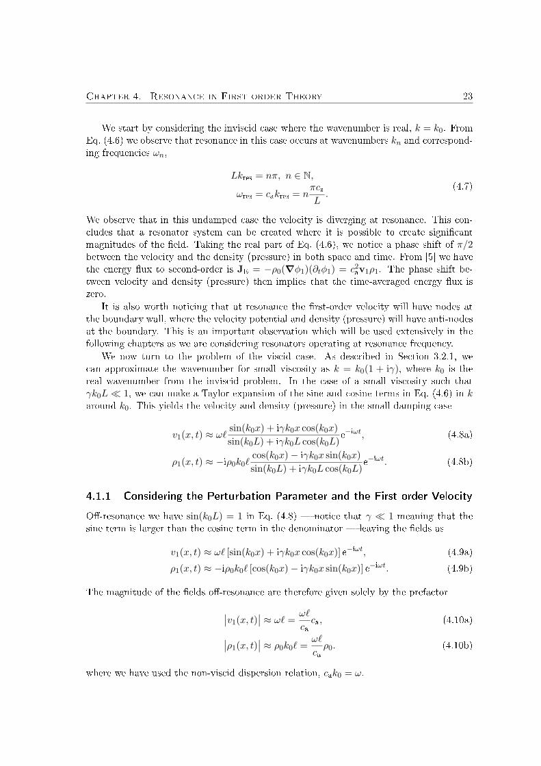
We start by considering the inviscid case where the wavenumber is real, k = k0. FromEq. (4.6) we observe that resonance in this case occurs at wavenumbers kn and correspond-ing frequencies ωn,
Lkres = nπ, n ∈ N,
ωres = cakres = nπcaL.
(4.7)
We observe that in this undamped case the velocity is diverging at resonance. This con-cludes that a resonator system can be created where it is possible to create significantmagnitudes of the field. Taking the real part of Eq. (4.6), we notice a phase shift of π/2between the velocity and the density (pressure) in both space and time. From [5] we havethe energy flux to second-order is JE = −ρ0(∇φ1)(∂tφ1) = c2av1ρ1. The phase shift be-tween velocity and density (pressure) then implies that the time-averaged energy flux iszero.
It is also worth noticing that at resonance the first-order velocity will have nodes atthe boundary wall, where the velocity potential and density (pressure) will have anti-nodesat the boundary. This is an important observation which will be used extensively in thefollowing chapters as we are considering resonators operating at resonance frequency.
We now turn to the problem of the viscid case. As described in Section 3.2.1, wecan approximate the wavenumber for small viscosity as k = k0(1 + iγ), where k0 is thereal wavenumber from the inviscid problem. In the case of a small viscosity such thatγk0L� 1, we can make a Taylor expansion of the sine and cosine terms in Eq. (4.6) in karound k0. This yields the velocity and density (pressure) in the small damping case
v1(x, t) ≈ ω`sin(k0x) + iγk0x cos(k0x)sin(k0L) + iγk0L cos(k0L)
e−iωt, (4.8a)
ρ1(x, t) ≈ −iρ0k0`cos(k0x)− iγk0x sin(k0x)sin(k0L) + iγk0L cos(k0L)
e−iωt. (4.8b)
4.1.1 Considering the Perturbation Parameter and the First-order Velocity
Off-resonance we have sin(k0L) = 1 in Eq. (4.8) — notice that γ � 1 meaning that thesine term is larger than the cosine term in the denominator — leaving the fields as
v1(x, t) ≈ ω` [sin(k0x) + iγk0x cos(k0x)] e−iωt, (4.9a)
ρ1(x, t) ≈ −iρ0k0` [cos(k0x)− iγk0x sin(k0x)] e−iωt. (4.9b)
The magnitude of the fields off-resonance are therefore given solely by the prefactor
∣∣v1(x, t)∣∣ ≈ ω` =ω`
caca, (4.10a)∣∣ρ1(x, t)
∣∣ ≈ ρ0k0` =ω`
caρ0. (4.10b)
where we have used the non-viscid dispersion relation, cak0 = ω.

24 Chapter 4. Resonance in First-order Theory
From Eq. (4.10) it is possible to read off the implicit perturbation factor discussed inSection 2.2. With characteristic parameter values we can estimate this to be
αoff,res =ω`
ca≈ 106 s−1 × 10⁻⁹ m
1483 m s−1= 6.7× 10⁻⁷. (4.11)
From this we conclude that off-resonance the perturbation approach is at least self consis-tent in the sense that it produces a perturbation parameter value α� 1.
Continuing from Eq. (4.8) at resonance, i.e. when the denominator is small, we getsin(k0L) = 0 and cos(k0L) = 1, indicating the resonance condition stated in Eq. (4.7). Atresonance we get the velocity and density (pressure) fields
v1(x, t) ≈ ω`[− i
nπγsin(knx) +
x
Lcos(knL)
], (4.12a)
ρ1(x, t) ≈ iρ0kn`
[i
nπγcos(knx) +
x
Lsin(knx)
]. (4.12b)
Comparing the fields off-resonance Eq. (4.9) and on-resonance Eq. (4.12) we notice that theresonance fields acquire a resonant component with an amplitude 1/(nπγ) ≈ 3.1×10⁴ (forn = 1) times larger than for the off-resonance field. This means a change in the magnitudeof the perturbation parameter in the resonant case
αres =1nπγ
ω`
ca≈ 3.1× 104 × 6.7× 10−7 = 2× 10⁻². (4.13)
We notice that with strong resonance, which in the limit goes towards the infinite inviscidcase treated above, we tend to invalidate the perturbation approach. Hence we concludethe importance of the viscosity of the fluid when regarding resonators. We also concludethat large energy resonances, corresponding to the case of very low viscosity, gives a pos-sible invalidation of the whole perturbation approach, which requires small values of theperturbation parameter, α� 1, to be valid.
It is also interesting to notice that the first-order velocity in this way is estimated tohave the magnitude |v1| ≈ 10−2ca at resonance. As pointed out in [22] this is about twomagnitudes higher than the experimentally observed values. This is primarily due to theassumption of a perfectly coupled and lossless resonator delivering its energy at resonance,which of course is not the case in the experimental setup. Like [22] we will as an estimateuse the experimentally confirmed magnitude |v1| ≈ 10−4ca, [33].
4.1.2 Energy in the Resonator
It can be shown that the acoustic energy density to second-order of the acoustic fields isgiven as the sum of the kinetic energy and the potential energy [5],
⟨Eac
⟩=
12ρ0
[⟨∇φ1
⟩2 +⟨ 1ca∂tφ1
⟩2]
=12ρ0
[⟨v2
1
⟩+⟨( ca
ρ0ρ1
)2 ⟩], (4.14)
where we in the last equality have used the relations between the first-order quantities andthe first-order velocity potential, cf. Eqs. (3.5) and (3.6).

Chapter 4. Resonance in First-order Theory 25
We will consider the general case including the viscosity. The expressions for the first-order velocity and density is then given in Eq. (4.8). Using the result for the time averageof harmonic variating quantities found in Section 3.5, and noticing that the real first-orderterms expressed by complex notation in Eq. (4.8) is found by taking the real part of thecomplex representation, we obtain
〈v21〉 =
12ω2`2
sin2(k0x) + γ2k20x
2 cos2(k0x)sin2(k0L) + γ2k2
0L2 cos2(k0L)
, (4.15a)⟨(caρ0ρ1
)2⟩
=12ω4`2
c2ak20
cos2(k0x) + γ2k20x
2 sin2(k0x)sin2(k0L) + γ2k2
0L2 cos2(k0L)
. (4.15b)
Inserting Eqs. (4.15a) and (4.15b) in Eq. (4.14) and using the Pythagorean identity forsines and cosines we get
⟨Eac
⟩=ρ0ω
2`2
41 + x2γ2k2
0
sin2(k0L) + γ2k20L
2 cos2(k0L), (4.16)
where we have also used the linear dispersion relation ω = cak0 and that we to first-orderin γ have k2 = k2
0 since γ � 1.We want to consider the spatial-averaged energy density in the resonator which is
located at x = −L to x = L. Hence we integrate the energy density over the length of theresonator,
ε =1
2L
∫ L
−L
⟨Eac
⟩dx =
ρ0ω2`2
8LL+ 1
3γ2k2
0L3
sin2(k0L) + γ2k20L
2 cos2(k0L). (4.17)
We can now expand the sine and cosine terms in the denominator again under the assump-tion that we are driving the resonator close to the resonance frequency ωres = cakres. TheTaylor expansions of the sine and cosine around the resonance frequency gives
sin(k0x) ≈ sin(ωresca
L
)+L
ca(ω − ωres) cos
(ωresca
L
), (4.18a)
cos(k0x) ≈ cos(ωresca
L
)− L
ca(ω − ωres) sin
(ωresca
L
). (4.18b)
Inserting the Taylor expansions Eqs. (4.18a) and (4.18b) into Eq. (4.17) while using theresonance condition Eq. (4.7) means that k0L ≈ kresL = ωresL/ca = nπ leading tosin (ωresL/ca) = 0 and cos (ωresL/ca) = (−1)n, and gives
ε =ρ0ω
2res`
2
81
L2/c2a (ω − ωres)2 + γ2L2ω2res/c
2a
(4.19)
=18ρ0c
2a
`2
L2
ωresγ
γωres
(ω − ωres)2 + γ2ω2res
, (4.20)
where we again use the assumption γ � 1 which is why the last term in the numerator ofEq. (4.17) can be neglected compared to the first one.

26 Chapter 4. Resonance in First-order Theory
We recognize the form of the energy density in the resonator Eq. (4.20) as a Lorentzian,which is the same kind of function we would get when solving for the amplitude of the clas-sical harmonic oscillator. The energy density is centered around the resonance frequencyωres and has a full width at half maximum (FWHM) of 2γωres. With the typical param-eters used in the following chapters FWHM around the resonance frequency is estimatedas
2γωres ≈ 2× 10−5 × 2π × 2× 106 rad s−1 = 40 Hz. (4.21)
This example of a resonator is one-dimensional and for a real analysis of the physical systemwe would of course have to generalize the analysis to three dimensions which is beyondthe scope of this thesis where we will not concentrate on the form of the resonance andhow it is actually created. An estimate can be given by considering the three-dimensionalcavity with homogeneous Neumann boundary because of the assumption of the walls beingacoustical hard materials so the pressure gradient is zero normal to the boundary walls,nnormal·∇p1 = 0. This leads to a restrictions on the frequencies determined by the geometry.In a rectangular cavity with the dimensions l0, w0, and h0 the solution to the Helmholtzequation with the mentioned boundary conditions gives the resonance frequencies as statedin [22],
ωres,3d = c2a
√(2πnl0
)2
+(
2πkh0
)2
+(
2πmw0
)2
, (n, k,m) ∈ N3. (4.22)

Chapter 5. Forces on Microparticles 27
Chapter 5
Forces Acting on Microparticles in
an Acoustic Field in an Inviscid
Fluid
Gor’kov [14] presented in 1962 a paper with derivations on a microparticle in an inviscidfluid under the influence of an acoustic field. This paper is very condensed, so in thischapter we would like to present a detailed derivation of Gor’kov’s results.
In the linear approximation described in Section 3.4, there can be no pressure force andhence in average no displacement of the particle, since all first-order terms are harmonicand are time-averaged to zero. Thus we have to go to second order to be able to see theseeffects. Below we derive an expression for the force acting on a small particle entrained bythe fluid in an arbitrary acoustic field. In the following chapter we will only be concernedwith inviscid fluids i.e. we are neglecting all loss terms and especially viscosity. Thisassumption is important since we want to describe the system by the velocity potentialwhich in turn demands that the fluid is isentropic. If the rotation is zero at one instantand the flow is not isentropic it will most certainly not be irrotational an instant later, seethe discussion in [16].
5.1 The Potential Flow
First we consider the constant flow around a particle in an acoustic field and want to de-termine if this flow is a potential flow. Using the Stokes theorem the irrotational conditioncan be written as zero circulation along any closed contour,∮
v· dl =∫
(∇× v)· dA = 0. (5.1)
From this it is clear that any constant velocity field is irrotational.
We need to determine if the flow around the particle is a potential flow. The isentropicflow is determined by the non-viscid Navier–Stokes equation, Eq. (2.1),
ρ [∂tv + (v ·∇)v] = −∇p. (5.2)
28 Chapter 5. Forces on Microparticles
If we follow the particle immersed in the fluid we have a system where the particle is notmoving but the fluid is. Because of the acoustical field the pressure oscillates making theparticle surface oscillate at a certain angular frequency ω and amplitude a.
The size of the individual terms of Eq. (5.2) are estimated as follows: The velocity of thefluid close to the particle surface changes by an amount of the same order as the velocity,u, of the oscillating surface of the particle over the characteristic size of the particle, l.This makes the spatial derivative of v of the order u/l and the term (v · ∇)v ∼ u2/l.Considering the first term in Eq. (5.2) we see that ∂tv is of the order ωu. Noticing thatthe angular frequency is of magnitude ω ∼ u/a we conclude that the first term is of theorder ∂tv ∼ u2/a. Comparing this to the other terms we obtain
|∂tv| � |(v ·∇)v| if a� l. (5.3)
We thus conclude that if the oscillations of the particle surface are small compared to thelength of the particle we can neglect the non-linear term of Eq. (5.2). This means that weare limited to only consider sufficiently small variations in the pressure so that the particlesurface is not vibrating with too large an amplitude.
Neglecting the second term of Eq. (5.2) and applying the rotation operator on bothsides yields ∇× (ρ∂tv) = −∇× (∇p) = 0 because the rotation of a gradient-field is zero.To first order ρ∂tv = ρ0∂tv1 which gives that ∇ × v1 is a constant with respect to time.Because rotation and time-average commute, 〈∇ × v1〉 = ∇ × 〈v1〉 is equal to the sameconstant. Assuming that v1 varies harmonically in time, we know that 〈v1〉 = 0 whichmeans that the constant also must be zero, giving ∇ × v1 = 0. Therefore to first orderthe pressure variation is sufficiently small so that the amplitude of the surface oscillationsof the particle is small compared to the particle size. The flow around the particle is apotential flow, and we can use the notation of velocity potential described in Chapter 3.
5.2 The Average Force For Second-order Perturbation
In the linear scattering theory we assume that the first-order velocity potential can bewritten as the sum of the wave incident on the particle, φin, and the scattered wave, φsc,
φ1(r, t) = φin(r, t) + φsc(r, t). (5.4)
This means that all interference effects are neglected. Furthermore, we are neglecting thescattered waves being reflected back towards the sphere from the wall of the fluid containeror other particles.
When neglecting body forces and viscid forces on the particle, the magnitude of theaverage force is equal to the average flux of momentum through any arbitrary closed surface∂V of the volume element V in which the particle is enclosed [5],
〈Fi〉 = −∫∂V〈Πij〉nj dA, (5.5)
where 〈Πij〉 = pδij + ρvivj is the time average of the momentum flux density tensor,nj = n · ej is the component of the outward pointing normal vector n to the surface in the

Chapter 5. Forces on Microparticles 29
direction of ej , and ρ is the density of the fluid. Using the perturbation scheme outlinedin Section 2.2 we include up to second-order effects for both the velocity and the pressure.
When neglecting viscosity we get the first-order perturbation in pressure from Eq. (3.7)
p1 = −ρ0∂tφ1. (5.6)
Restricting ourselves to periodic time variating first-order perturbations, we observe that〈p1〉 = 0 by Eq. (3.47).
The second-order time-average perturbation of the pressure is obtained from Eq. (3.51),and noticing that the second-order expansion of ρvivj is ρ0v1,iv1,j , we can rewrite Eq. (5.5)as
〈Fi · ei〉 = −∫∂V
{[−ρ0〈v2
1〉2
+ρ0
2c2a
⟨(∂tφ1)2
⟩]δij + ρ0〈v1,iv1,j〉
}nj dA. (5.7)
We see from Eq. (5.7) that we only need to solve the linear scattering problem, i.e. deter-mine φ1, to determine the force. We therefore dedicate the next section to determinationof the velocity potential.
5.2.1 Calculation of the Velocity Potential
In Chapter 3 we saw that the velocity potential fulfilled the scalar wave equation Eq. (3.8).Making a multipole expansion of the solution, see Appendix B, taking into account onlythe terms which are not diverging at infinity, we look for retarded solutions φsc to thevelocity potential of the form
φsc =a(t− r/ca)
r+ ∇·
(A(t− r/ca)
r
)+ · · · (5.8)
=a(t− r/ca)
r− A(t− r/ca) · er
car− A(t− r/ca) · er
r2+ · · · . (5.9)
Here and in the following the dot denotes the derivative with respect to the argument.Assuming that A varies periodically in time with angular frequency ω, then A/ca ∼Aω/ca ∼ A/λ. This means that in the region close to the particle i.e. r � λ, we look forsolutions of the form
φsc =a(t)r− A(t) · er
r2+ · · · , (5.10)
where er is a unit vector pointing in the radial direction. This corresponds to only includingthe largest of the two terms including A in Eq. (5.9). Notice that Eq. (5.10) is for small rvalues.
We now look at the situation close to the particle where Eq. (5.9) reduces to Eq. (5.10),to determine the coefficients a and A. To do this we make a general simplification of theproblem. Until now we have been discussing particles of an arbitrary shape. Now wesimplify our problem to spherically shaped particles in order to be able to determine thecoefficients. In all of the following we will therefore only be concerned with sphericallyshaped particles.
The strategy for determining the coefficients is to consider different situations whereeither the first or the second term of Eq. (5.10) vanish, and we therefore can determine theother coefficient.

30 Chapter 5. Forces on Microparticles
First Term — Mass Flux
We now consider the first term a(t)/r of Eq. (5.10). This term describes the ejection ofthe fluid because of the presence of the sphere and the compressibility of the sphere. Wetherefore consider a stationary sphere in the fluid in an acoustic field which to first-order iscarrying the density ρin at the location of the sphere. This problem has complete rotationalsymmetry and hence the term including A vanish because we see that this term includesan angular dependence. It therefore suffices to consider only the first term of Eq. (5.10)for this setup.
First we look at an incompressible sphere of radius R and volume Vs. The volumeVsρin/ρ0 would have entered the volume now occupied by the sphere per unit time. Thisvolume would have entered if the sphere was absent and is equivalent to the emission ofthe same volume from the surface of the sphere by the scattered wave. If the normal vectorer is taken as pointing outwards, this means that
Vsρin(t)ρ0
=∫∂Vs
vsc(t) · er dA. (5.11)
Because vsc = ∇φsc the integral becomes
4π3R3 ρin(t)
ρ0=∫∂Vs
∇φsc ·er dA (5.12)
=∫∂Vs
∇(a(t)r
)·er dA (5.13)
= −∫∂Vs
a(t)r2
er ·er dA (5.14)
= −a(t)R2
4πR2. (5.15)
Thus
a(t) = − R3
3ρ0ρin(t). (5.16)
We can expand this derivation by taking into account the fact that the sphere is compress-ible. It means that Eq. (5.11) becomes
Vsρin(t)ρ0
+ δVs,1 = −4πa(t), (5.17)
where δVs,1 denotes the first-order volume change per unit time due to compression of thesphere.
We now take advantage of the fact that δVs,1 by definition is small, since we only areconsidering the case where the amplitude of the oscillations of the surface is small comparedto the length scale of the particle. This means that we can express it using the chain rule,
δVs,1 =∂Vs∂ρs
∂ρs∂ps
δps,1, (5.18)
Chapter 5. Forces on Microparticles 31
where it is understood that the process of changing the volume of the sphere must beisentropic, so we keep considering a lossless system. In analogy with Eq. (2.6) we definethe speed of sound in the sphere as the isentropic derivative,
c2s =(∂ps∂ρs
)ρ=ρs
. (5.19)
Because the pressure outside the sphere must be the same as inside the sphere at equi-librium we notice from Eq. (2.8c) that the first-order perturbation of the pressure, δps,1,is
δps,1 = p1 = c2aρ1 = c2aρin ⇒ δps,1 = c2aρin. (5.20)
Furthermore, using that
∂Vs∂ρs
=∂
∂ρs
(ms
ρs
)= −ms
ρ2s
= −Vsρs, (5.21)
with ms denoting the mass of the sphere, Eq. (5.18) becomes
δVs,1 = −Vsρinc
2a
ρsc2s. (5.22)
From Eq. (5.17) we finally obtain a(t),
a(t) = − 14π
(Vsρin(t)ρ0− Vs
ρinc2a
ρsc2s
)= − R
3
3ρ0˙ρin(t)
(1− ρ0c
2a
ρsc2s
). (5.23)
This takes into account both the volume that the sphere occupies and thereby the masswhich is expelled from the surface and the fact that the sphere changes size when placedin the fluid in an acoustic field.
These effects are present no matter if the sphere is stationary or moving, as long as thereis an incoming density perturbation of the size ρin, and a following pressure perturbationto make the surface compress.
Second Term — Movement of the Sphere and Fluid in Presence of the Sphere
The second term in Eq. (5.10) can be determined from the fact that in a stationary flow thenormal component of the velocity of the fluid and the normal component of the velocity ofthe surface must be the same for r = R. We consider a sphere moving with the constantvelocity vs in a stationary fluid. This problem clearly involves a direction and hence anangular dependence. The first term of Eq. (5.10) does not exhibit any angular dependence,so for this kind of problem it suffices to only consider the second term. Though the effectsdescribed above concerning mass flux is still valid, these effects cannot have any influenceon the flow of the fluid around the sphere.
The mentioned continuity condition for the normal component of the velocity of thefluid and the velocity of the surface of the sphere, means that only the radial part of A(t)enters the equations. Neglecting all other parts we can write A(t) = Ar(t)er, remembering

32 Chapter 5. Forces on Microparticles
that the fluid velocity is given as ∇φsc and only taking the radial part of the gradient, weget
vs · er = ∇(−A · er
r2
)· er∣∣∣∣r=R
= Ar2erR3· er. (5.24)
Thus A(t) · er = 1/2vs · erR3, and the second term of φsc in Eq. (5.10) becomes
− A(t) · err2
= −vs · erR3
2r2. (5.25)
In general, the fluid is not stationary, but both the fluid and the sphere is moving, implyingthat the sphere is entrained by the fluid and moves with a velocity u(t). We notice that itstill suffices only to consider the second term of Eq. (5.10) since this problem still involvesdirections.
Since the equation for the full potential, Eq. (5.4), is linear and fulfills the scalar waveequation as described in Chapter 3, so must the scattered potential,
∇2φsc =1c2a∂ 2t φsc. (5.26)
We notice that for a sphere with radius R the velocity potential changes notably overthis length scale, hence the spatial derivative in the left-hand side of Eq. (5.26) is ofthe order ∼ φsc/R
2. The right-hand side is for harmonic time dependence of the order∼ ω2φsc/c
2a ∼ φsc/λ
2. For high frequency acoustic waves, and close enough to the sphere,we have the condition λ� R, and we can neglect the right-hand side of Eq. (5.26) whichleads to that close to the sphere, the velocity potential must obey the Laplace equation,∇2φsc = 0.
To determine the coefficient A we consider the situation close to a sphere entrainedby the fluid, when the fluid has a constant velocity and flows in the x-direction. Hencewe solve the Laplace equation inside and outside the sphere. Denoting the scattered fieldoutside with subscript O and inside the sphere with subscript I, the Laplace problem issubject to the following boundary conditions:
BC 1 Continuity of the pressure, pI = pO at r = R. To first order in Eq. (3.7) we getpsc = p0− ρ0∂tφsc = ρ0 +iρ0ωφsc, assuming that the time-dependence is on the forme−iωt. This means that
ρI∂tφI = ρO∂tφO ⇒ ρIφI = ρOφO, at r = R, (5.27)
BC 2 Continuity of the normal velocity
vI · er = vO · er ⇒ ∂rφI = ∂rφO, at r = R. (5.28)
BC 3 φO(r, θ) → vinr cos θ for r → ∞; far from the sphere the scattered velocity fieldmust be like the incoming field.
BC 4 φI must remain finite.

Chapter 5. Forces on Microparticles 33
Using boundary condition 3 we see that the potential only can have a cosine variation(not higher powers of cos θ). This gives the following linear combination of solutions to∇2 {rp cos θ} = 0 with p being an integer
φ(r, θ) =[Ar +Br−2
]cos θ. (5.29)
Inside the sphere the potential cannot diverge according to boundary condition 4, thusBI = 0, and φI must have the form
φI(r, θ) = AIr cos θ. (5.30)
Similarly using boundary condition 3 we conclude that AO = vin so that the potentialoutside the sphere must have the form
φO(r, θ) =[vinr +BOr
−2]cos θ. (5.31)
Using boundary conditions 1 and 2, respectively we arrive at the two equations
ρIAIR = ρO(vinR+BOR
−2)
(5.32a)
AI = vin − 2BOR−3. (5.32b)
By solving Eq. (5.32) with respect to AI and BO we find the potential to be given as
φI(r, θ) = vinr3ρO
2ρI + ρOcos θ, (5.33a)
φO(r, θ) = vin
[r +
ρI − ρO2ρI + ρO
R3r−2
]cos θ. (5.33b)
Identifying that ρ0 = ρO and ρs = ρI as the density of the fluid and the sphere respectivelyand using that vinr cos θ = vin · r, we see that the velocity potential inside the sphere φIgives the velocity of the sphere itself. Taking the gradient of φI, we get the velocity u(t)of the sphere entrained by the fluid with the constant velocity vin,
u(t) = ∇φI =3ρ0
2ρs + ρ0vin(t). (5.34)
We see that we have to correct Eq. (5.25) now that the fluid is also moving around thesphere. Placing ourselves in the reference frame of the fluid we again obtain a situationwhere the fluid is at rest with respect to the chosen coordinate system and the sphere ismoving. This situation determines A(t) as shown in Eq. (5.25) where vs is the velocity ofthe sphere in the chosen system. In the rest-frame of the fluid the sphere will, accordingto Eq. (5.34), have the velocity vin(t)− u(t) giving the coefficient as
A(t) = −[vin(t)− u(t)
]R3
2= −R
3(ρs − ρ0)2ρs + ρ0
vin(t). (5.35)
Using the constants a and A found in Eq. (5.23) and Eq. (5.35) we get the scatteredvelocity potential by inserting into the general solution Eq. (5.8),
φsc(t− r/ca) = − R3
3ρ0rρin(t− r/ca)f1 −
R3
2f2∇ ·
(vin(t− r/ca)
r
), (5.36)
where
f1 = 1− ρ0c2a
ρsc2sand f2 =
2(ρs − ρ0)2ρs + ρ0
. (5.37)
34 Chapter 5. Forces on Microparticles
5.3 Forces Acting on a Particle in a Plane Running Wave
We want to determine the force on particles in an ideal fluid when the incoming acousticfield is a plane traveling monochromatic wave in the x-direction
φin(x, t) = −u0
kcos(kx− ωt). (5.38)
Furthermore, we still use the linear approximation for the full first-order perturbation ofthe velocity potential,
φ1(r, t) = φin(r, t) + φsc(r, t), (5.39)
implying that all quantities with the subscript „in” or „sc” is of first-order.We see that the projection of the force in the x-direction is given from Eq. (5.7) by an
integral over the surface of the sphere (r = R)
〈Fx〉 = 〈F · ex〉 =−∫∂V
{[−ρ0〈v2
1〉2
+ρ0
2c2a
⟨(∂φ1
∂t
)2⟩]ex · er
+ ρ0
⟨(ex · v1)(v1 · er)
⟩}dA.
(5.40)
When inserting the linear splitting of the potential in incoming and scattered quantitiesindicated in Eq. (5.39), the first term in the curly brackets becomes
ζ =
[−ρ0〈v2
1〉2
+ρ0
2c2a
⟨(∂φ1
∂t
)2⟩]cos θ, (5.41a)
or
ζ =ρ0
2
[−⟨v2in,0 + v2
sc,0 + 2vin,0vsc,0 cos θ⟩
+1c2a
⟨(∂tφin)
2 + (∂tφsc)2 + 2(∂tφin)(∂tφsc)
⟩]cos θ.
(5.41b)
Here, we have introduced the angle θ between the radial direction, er, and the x direction,ex, and used vin,0 to denote the amplitude of the incoming velocity i.e. vin = vin,0ex,and vsc,0 to denote the amplitude of the radial component of the scattered velocity i.e.
vsc = vsc,0er.In Appendix C we have calculated the scattered and incoming velocity field created
because of the incoming potential Eq. (5.38). In Eqs. (C.3) and (C.13) we found that∂tφin = −cavin,0 and ∂tφsc = −cavsc,0. Using this in Eq. (5.41b) we conclude that
ζ =ρ0
2
[−⟨v2in,0 + v2
sc,0 + 2vin,0vsc,0 cos θ⟩
+1c2a
⟨(−cavsc,0)2 + (−cavin,0)2 + 2(−cavin,0)(−cavsc,0)
⟩]cos θ,
(5.42a)
= ρ0vin,0vsc,0(cos θ − cos2 θ
). (5.42b)

Chapter 5. Forces on Microparticles 35
The second term in the integrand of Eq. (5.40) is
ρ0
⟨(ex · v1)(v1 · er)
⟩= ρ0
⟨(ex · [vin + vsc]) ([vin + vsc] · er)
⟩(5.43)
= ρ0
⟨(vin,0 + vsc,0 cos θ)(vin,0 cos θ + vsc,0)
⟩(5.44)
= ρ0
⟨v2in,0 cos θ + v2
sc,0 cos θ + vin,0vsc,0(1 + cos2 θ)⟩. (5.45)
Thus the average force on the particle in the direction of the incoming wave (x-direction)is found by inserting Eq. (5.42b) and Eq. (5.45) into Eq. (5.40),
〈Fx〉 = −ρ0
∫∂V
⟨v2in,0 cos θ + v2
sc,0 cos θ + vin,0vsc,0(1 + cos θ)⟩dA. (5.46)
To reduce the expression even further and to realize that the force from a plane travelingwave only depends on the momentum carried away by the scattered wave, we consider thechange of energy inside a given volume. Following [5] we find that the change in energywith time inside a given volume V is given by the change in energy flux,∫
V∂tEacdV = −
∫V
∇ · JEdV. (5.47)
Taking the time average of Eq. (5.47), remembering that the time average of a time deriva-tive is always zero for periodic functions, see Eq. (3.47), we arrive at
0 =⟨∫
V∂tEacdV
⟩=⟨∫
V∇ · JEdV
⟩=⟨∫
∂VJE ·dA
⟩=∫∂V〈JE〉·dA, (5.48)
where we have used Gauss’s theorem to convert the volume integral into a surface integraland without loss of generality assumed that the surface does not vary in time. From [5]we have that the energy flux to second order is given as
JE = ρ0 (∇φ1) (∂tφ1) = ρ0v1 (∂tφ1) , (5.49)
where the subscript 1 as usual denotes the first-order perturbation quantities.Now we use the linear splitting of the first-order quantities and exploit Eq. (5.48) to
get a useful relation between the scattered and incoming velocity components if we let theconsidered surface be a sphere
0 =∫∂V
⟨ρ0
(∂φin∂t
+∂φsc∂t
)v1
⟩· dA (5.50a)
= ρ0
∫∂V
⟨(−cavin,0 − cavsc,0)(vin,0ex + vsc,0er)
⟩·er dA (5.50b)
= ρ0ca
∫∂V
⟨[v2in,0 cos θ + v2
sc,0 + vin,0vsc,0(1 + cos θ))]⟩
dA (5.50c)
=⟨v2in,0 cos θ + v2
sc,0 + vin,0vsc,0(1 + cos θ)⟩, (5.50d)

36 Chapter 5. Forces on Microparticles
where we again have used the relations from Appendix C, ∂tφsc = −cavsc,0 and ∂tφin =−cavin,0. The last equation follows from the arbitrary choice of integration surface. If theintegral is zero for an arbitrary choice of surface, then the integrand must be identical zero.Using Eq. (5.50d) to reduce Eq. (5.46), the average force turns out to be
〈Fx〉 = ρ0
∫∂V〈v2
sc,0〉(1− cos θ) dA. (5.51)
The scattered velocity that emerges from the incoming potential Eq. (5.38) throughthe use of Eq. (5.36) is calculated in Appendix C to lowest order in r
vsc(t− r/ca) =R3u0ω
2
c2arsin[ω(t− r/ca)
](13f1 −
12f2 cos θ
)er +O(r−2). (5.52)
Using that the time average of a sine function squared over a full period is 1/2, we get thedesired time average,
〈v2sc,0〉 =
⟨[R3u0ω
2
c2arsin(ω(t− r/ca))
(13f1 −
12f2 cos θ
)]2⟩(5.53a)
=R6u2
0ω4
2c4ar2
(13f1 −
12f2 cos θ
)2
. (5.53b)
We can now evaluate the integral in Eq. (5.51),
〈Fx〉 = 2πρ0R
6u20k
4
2
∫ π
0
[1R2
(f21
9− f1f2
3cos θ +
f22
4cos2 θ
)
× (1− cos θ)R2 sin θ
]dθ
(5.54a)
=ρ0R
6u20k
4
22π
29
(f21 + f1f2 +
34f22
). (5.54b)
Letting I = ρ0cau20/2 denote the average energy flux density, the average force on a spher-
ical particle with radius R in a fluid in a monochromatic wave is
〈Fx〉 =4πI9ca
R2(kR)4(f21 + f1f2 +
34f22
). (5.55)
We see that the force scales as k4. This implies that this force is very small forrapidly oscillating incoming waves. Because we are operating at ultrasound frequenciesf & 1.5 MHz, we conclude that this force is negligible. In the next section we thereforeconsider the force in an arbitrary wave which is not similar to the plane running wave.

Chapter 5. Forces on Microparticles 37
5.4 Forces Acting on a Particle in an Arbitrary Wave
We neglect second-order terms in the scattered and incoming wave thus only taking intoaccount the mixed terms. This reduces Eq. (5.7) to
〈Fi〉 = −∮ ([
−ρ0
2〈v2
1〉+ρ0
2c2a
⟨(∂tφ1)2
⟩]δik + ρ0〈v1,jv1,k〉
)nk dA (5.56a)
= −ρ0
∮ ([− 1
2⟨(vsc + vin)2
⟩+
ρ0
2c2a
⟨[∂t(φsc + φin)]2
⟩]δik
+ ρ0
⟨(vsc,i + vin,i)(vsc,k + vin,k)
⟩)nkdA
(5.56b)
= −∮ ([
−ρ0
2⟨2vsc,jvin,j
⟩+
ρ0
2c2a
⟨2(∂tφsc)(∂tφin)
⟩]δik
+ ρ0
⟨vsc,ivin,k + vin,ivsc,k
⟩)nkdA.
(5.56c)
Remembering that ρ1 = −ρ0/(c2a)∂tφ1 from Eq. (3.6) we get for the average force to firstorder in the scattered and incoming waves
〈Fi〉 = −∮ ([
−ρ0〈vsc,jvin,j〉+c2aρ0〈ρscρin〉
]δik + ρ0〈vsc,ivin,k〉+ ρ0〈vin,ivsc,k〉
)nkdA.
(5.57)We convert expression (5.57) to a volume integral using the Gauss’s theorem and thatsummation over all k is implicit,
〈Fi〉 = −∫V∂k
([−ρ0〈vsc,jvin,j〉+
c2aρ0〈ρscρin〉
]δik
+ ρ0〈vsc,ivin,k〉+ ρ0〈vin,ivsc,k〉)dV,
(5.58)
Noticing that time average and spatial differentiation commute, we get
〈Fi〉 = −∫V
[− ρ0〈(∂ivsc,j)vin,j〉 − ρ0〈vsc,j(∂ivin,j)〉+
c2aρ0〈(∂iρsc)ρin〉+ 〈ρsc(∂iρin)〉
+ ρ0 (〈(∂kvsc,i)vin,k〉+ 〈vsc,i(∂kvin,k)〉+ 〈(∂kvin,i)vsc,k〉+ 〈vin,i(∂kvsc,k)〉)]dV.
(5.59)
We note that we are considering a potential flow, and thus
∂kvj = ∂k∂jφ = ∂j∂kφ = ∂jvk. (5.60)

38 Chapter 5. Forces on Microparticles
Using this interchange of the indices in Eq. (5.59), we get
〈Fi〉 =−∫V
{c2aρ0
[⟨(∂iρsc)ρin
⟩+⟨ρsc(∂iρin)
⟩]
+ ρ0
[⟨vsc,i(∂kvin,k)
⟩+⟨vin,i(∂kvsc,k)
⟩]}dV.
(5.61)
We now consider the inviscid first-order governing equations, Eq. (3.1a) and Eq. (3.1b).Using the linear splitting of the first-order quantities in a scattered and an incoming part,as shown for the potential in Eq. (5.39), we can write the governing first-order equationsas [
ρ0∂t(vsc + vin)]i=[− c2a∇(ρsc + ρin)
]i= −c2a∂i(ρsc + ρin), (5.62a)
∂t(ρsc + ρin) = −ρ0∇·(vsc + vin) = −ρ0∂k(vsc,k + vin,k). (5.62b)
From Eq. (5.62a) we conclude that
∂iρsc = −ρ0
c2a∂t(vsc,i + vin,i)− ∂iρin, (5.63a)
∂iρin = −ρ0
c2a∂t(vsc,i + vin,i)− ∂iρsc, (5.63b)
and from Eq. (5.62b) we see that we can write
ρ0∂kvin,k = −∂t(ρsc + ρin)− ρ0∂kvsc,k. (5.64)
Exploiting Eqs. (5.63a), (5.63b), and (5.64) we reduce Eq. (5.61) to
〈Fi〉 =−∫V
{⟨(−∂t(vsc,i + vin,i)−
c2aρ0∂iρin
)ρin
⟩+⟨ρsc
(−∂t(vsc,i + vin,i)−
c2aρ0∂iρsc
)⟩
+⟨vsc,i(−∂t(ρsc + ρin)− ρ0∂kvsc,k)
⟩+ ρ0
⟨vin,i(∂kvsc,k)
⟩}dV.
(5.65)
We emphasize that we are only considering first-order perturbations in the scattering andincoming fields, i.e. we are only considering mixed terms in the scattered and incomingfields. This reduces Eq. (5.65) to
〈Fi〉 = −∫V
{−⟨ρin(∂tvsc,i)
⟩−⟨ρsc(∂tvin,i)
⟩−⟨vsc,i(∂tρin)
⟩+ ρ0
⟨vin,i(∂kvsc,k)
⟩}dV
(5.66a)
= −∫V
{−⟨∂t(ρinvsc,i)
⟩−⟨ρsc(∂tvin,i)
⟩+ ρ0
⟨vin,i(∂kvsc,k)
⟩}dV. (5.66b)

Chapter 5. Forces on Microparticles 39
We notice the general case of the time average of a time derivative of an arbitrary periodicfunction i.e.,
⟨∂tf⟩
= 0, see Eq. (3.47). For periodic first-order perturbations we thereforeget ⟨
∂t(ρinvsc,i)⟩
=⟨∂t(ρscvin,i)
⟩=⟨ρsc(∂tvin,i) + (∂tρsc)vin,i
⟩= 0, (5.67)
or ⟨ρsc(∂tvin,i)
⟩= −
⟨(∂tρsc)vin,i
⟩. (5.68)
Inserting Eqs. (5.67) and (5.68) into Eq. (5.66b) we get
〈Fi〉 = −∫V
⟨vin,i (ρ0(∂kvsc,k) + ∂tρsc)
⟩dV. (5.69)
Reintroducing the velocity potential by the relations vsc,k = ∂kφsc and ρsc = −ρ0/(c2a)∂tφsc,we get
〈Fi〉 = −ρ0
∫V
⟨vin,i
[∂ 2k φsc −
1c2a∂ 2t φsc
]⟩dV. (5.70)
If we consider the integrand of Eq. (5.70) we see that the contents of the squared bracketsare similar to the wave equation for the scattered velocity potential, Eq. (5.26). Thescattered velocity potential has been determined in Eq. (5.36). We conclude that we areconsidering the case described in Appendix B with
a(t− r/c) = −R3/(3ρ0)f1ρin(t− r/c), (5.71)
and
A(t− r/c) = −R3/(2)f2vin(t− r/c). (5.72)
From the analogy with Appendix B we see from Eqs. (B.13) and (B.24) that inserting thevelocity potential Eq. (5.36) into the scalar wave equation will give us zero everywhereexcept at the origin, where the divergence is represented by delta-functions. As usualsuppressing the arguments, we see that[
∇2 − 1c2a∂ 2t
] [a
r+ ∇·
(Ar
)]= −4πaδ3(r)− 4π∇·
[Aδ3(r)
](5.73)
= 4πR3
3ρ0f1ρinδ
3(r) + 4πR3
2f2∇·
[vinδ3(r)
]. (5.74)
Inserting Eq. (5.74) into Eq. (5.70), we get
〈Fi〉 = −ρ0
∫V
⟨vin,i
[4π3ρ0
R3f1ρinδ3(r) + 2πR3f2∇·
(vinδ3(r)
)]⟩dV. (5.75)
Remembering the general rules for integration by parts,∫V
(∇f) · u dV =∫∂V
fu·dA−∫Vf(∇·u)dV, (5.76)

40 Chapter 5. Forces on Microparticles
where f is an arbitrary scalar function and u is an arbitrary vector function, we can nowcarry out the integration1 in Eq. (5.75) with f = vin,i and u = vinδ3(r)
〈Fi〉 =− ρ0
⟨4π3ρ0
R3f1ρinvin,i
⟩− 2πR3f2ρ0
[ ∫∂V
⟨vin,ivinδ3(r)
⟩·dA
−∫V
⟨(∇vin,i) · vinδ3(r)
⟩dV
].
(5.77)
Here we take the volume to be any volume outside the considered body, because we bydefinition have placed the origin inside the body.
The first integral in the squared brackets is zero because the integration area does notinclude the origin, and the three-dimensional delta function therefore is zero everywhereon the integration surface. Hence we get
〈Fi〉 = −43πR3f1
⟨ρinvin,i
⟩+ 2πR3f2ρ0
⟨(∇vin,i)·vin
⟩(5.78)
= −43πR3f1
⟨ρinvin,i
⟩+ 2πR3f2ρ0
⟨(∂kvin,i)vin,k
⟩. (5.79)
In Eq. (5.79) it is understood that every variable is taken at the origin, i.e. at the positionof the particle in consideration.
To make the interpretation of this result more simple we want to express the averageforce by a force potential. We notice that we have assumed the first-order velocity per-turbation to be an irrotational vector field, hence by Eq. (5.79) the average force mustalso be an irrotational vector field. We can therefore introduce the scalar force potentialin analogy to the velocity potential as 〈F〉 ≡ −∇U . Notice that the minus sign is purelyconventional to make particles go to places with a small potential.
We notice that we can rewrite the first term of Eq. (5.79) when we only consider periodicperturbations. From Eq. (3.47) we conclude that⟨
∂t(ρinvin)⟩
= 0 (5.80)
or ⟨(∂tρin)vin
⟩= −
⟨ρin(∂tvin)
⟩. (5.81)
Using the result Eq. (5.80) and the governing equations without viscosity, Eq. (3.1a) andEq. (2.8c), we can rewrite the first term of Eq. (5.79) to concern only the pressure,
−43πR3f1
⟨(∂tρin)vin,i
⟩=
43πR3f1
⟨ρin(∂tvin,i)
⟩=
43πR3f1
⟨(pinc2a
)(−∂ipin
ρ0
)⟩(5.82a)
= − 43c2aρ0
πR3f1
⟨pin (∂ipin)
⟩. (5.82b)
1Integration of the three-dimensional δ-function is defined as:∫
Vf(r)δ3(r − r0)dV = f(r0) if the
volume V includes the point r = r0, otherwise the integral equals zero.
Chapter 5. Forces on Microparticles 41
When we want to write the force as the gradient of the scalar force potential, we noticethat
∂i(p2in) = 2pin(∂ipin), (5.83a)
∂i(v2in) = 2vin,k(∂ivin,k) = 2vin,k(∂kvin,i), (5.83b)
where we in the last equality in Eq. (5.83b) have used the assumption that the velocityfield is irrotational, and that we therefore can interchange the indices when taking thegradient as shown in Eq. (5.60).
We notice that Eq. (5.83a) and Eq. (5.83b) are the expressions that we have in Eq. (5.79).Using this and the result from Eq. (5.82b), we see that the force can be written as thegradient of a scalar field,
〈Fi〉 = − 43c2aρ0
πR3f1
⟨pin (∂ipin)
⟩+ 2πR3f2ρ0
⟨(∂kvin,i)vin,k
⟩(5.84a)
= − 43c2aρ0
πR3f1
⟨12∂i(p
2in)⟩
+ 2πR3f2ρ0
⟨12∂i(v
2in)⟩. (5.84b)
This implies that the scalar field U for which 〈F〉 = −∇U is given as
U =2
3c2aρ0πR3f1
⟨p2in
⟩− πR3f2ρ0
⟨v2in
⟩= 2πR3ρ0
[ ⟨p2in
⟩3c2aρ2
0
f1 −⟨v2in
⟩2
f2
]. (5.85)
5.5 Pressure Force on a Single Particle in a Standing Wave
Eq. (5.85) is expressing the force potential on a body given the incoming pressure pin andvelocity vin at the position of the particle. Assuming a standing wave in a single direction,the x-direction, we can write the incoming velocity potential as
φin =u0
kcos(kx) cos(ωt), (5.86)
where u0 is the velocity amplitude, k is the wavenumber of the standing wave, and ω isthe angular frequency of the wave. From Eqs. (3.5) and (3.7) we get the velocity and thepressure
vin = ∇φin = (∂xφin)ex = −u0 sin(kx) cos(ωt)ex, (5.87a)
pin = −ρ0∂tφin =u0ρ0ω
kcos(kx) sin(ωt) = u0ρ0ca cos(kx) sin(ωt). (5.87b)
Inserting Eqs. (5.87a) and (5.87b) into Eq. (5.85) gives the force potential
U = 2πR3ρ0
[⟨(u0ρ0ca)2 cos2(kx) sin2(ωt)
⟩3c2aρ2
0
f1 −⟨u2
0 sin2(kx) cos2(ωt)⟩
2f2
](5.88a)
= 2πR3ρ0u20
[13f1
⟨cos2(kx) sin2(ωt)
⟩− 1
2f2
⟨sin2(kx) cos2(ωt)
⟩](5.88b)
= 2πR3ρ0u20
[16f1 cos2(kx)− 1
4f2 sin2(kx)
], (5.88c)

42 Chapter 5. Forces on Microparticles
where we in the last equality have used that the time-average of cosine or sine functionsover a period is 1/2.
The average force on a particle located at x is then given as 〈Fx〉 = −∂xU , from thedefinition 〈F〉 = −∇U , which leads to
〈Fx〉 = −2πR3ρ0u20
[−2
6f1k cos(kx) sin(kx)− 2
4f2k sin(kx) cos(kx)
](5.89a)
= −4πR3ρ0u20k cos(kx) sin(kx)
[−1
6f1 −
14f2
](5.89b)
= 8πkR3〈Eac〉 sin(2kx)[16f1 +
14f2
], (5.89c)
where we in the last equality have used the trigonometric identity sin(2a) = 2 sin(a) cos(a)and the dispersion relation ω = cak. Furthermore we have used that the average acousticenergy in the incoming wave 〈Eac〉 is given by [5]
〈Eac〉 =12ρ0
[⟨(∇φin)2
⟩+⟨(
1ca∂tφin
)2⟩](5.90a)
=12ρ0
[⟨(−u0 sin(kx) cos(ωt))2
⟩+
⟨(−u0ω
kcacos(kx) sin(ωt)
)2⟩]
(5.90b)
=14ρ0
[u2
0 sin2(kx) + u20 cos2(kx)
]=
14ρ0u
20. (5.90c)
Returning to Eq. (5.89c) inserting Eq. (5.37) gives the force acting on a small particle ina standing wave in the x-direction:
〈Fx〉 = 8πkR3〈Eac〉 sin(2kx)[16
(1− c2aρ0
c2sρs
)+
14
2(ρs − ρ0)2ρs + ρ0
](5.91a)
= 4πkR3〈Eac〉 sin(2kx)
[ρs + 2
3(ρs − ρ0)2ρs + ρ0
− 13c2aρ0
c2sρs
](5.91b)
= 4πkR3〈Eac〉Φ sin(2kx). (5.91c)
We see by comparison with Eq. (5.55) that this force is many times larger because it scalesas (kR)R2 and not as (kR)4R2 which was the case for the plane traveling wave. Forsimplicity we define the term in the square brackets in Eq. (5.91b) as Φ.
5.6 Visualizing the Pressure Force and the Idea Behind Par-
ticle Separation
When we in the following chapters discuss the acoustophoretic sign, we understand it asthe sign of the Φ-factor. We notice that it is the Φ-factor which determines the directionof the pressure force. Hence it is the density and speed of sound of the single particlescompared to the fluid that determines the direction of the pressure force.

Chapter 5. Forces on Microparticles 43
0 y=ww/2
Pressure, p
F when Φ>0
F when Φ<0
Force, F
Figure 5.1: A sketch showing the pressure (velocity potential) standing wave in the channel witha wavelength of λ/2 = w. Furthermore the resulting pressure force as expressed by Eq. (5.91c) issketched for Φ > 0. If we plotted it for Φ < 0 the sign would change. The arrows indicate thedirection of the force on particles with negative or positive Φ-factor respectively.
As an illustration of the principle we consider a resonator of the type discussed inChapter 4 where the walls are placed at y = 0 and y = w. At resonance the pressurefield (velocity potential) has anti-nodes at the walls as shown in Eq. (4.6). The wavelengthis then given as λ/2 = w which gives the fundamental mode of the resonance conditionderived in Eq. (4.7), k = nπ/w, n ∈ N. We see from Fig. 5.1 that the wavelength ofthe force is half the wavelength of the pressure resulting in a positive force in the area0 < y < w/2 and a negative force for w/2 < y < w for particles with Φ > 0. The resultis that particles with a positive Φ-factor move towards the center of the channel and arethereby collected at the nodes in the pressure. In the same way we observe that particleswith Φ < 0 move towards the edges of the channel and end up at the anti-nodes in thepressure. It is this general principle we will be using in order to separate different types ofparticles in the second part of the thesis.
5.7 Considering the Pressure Force in 2D
The pressure force can also be determined in the two-dimensional case where we use thepotential from Eq. (5.85) as a starting point. When considering a standing wave in twodimensions, we can write the velocity potential corresponding to Eq. (5.86) as
φ2Din =u0
kcos(kxx) cos(kyy) cos(ωt), (5.92)
where we use the fact that a standing wave can be written as the sum of two counter-propagating waves with wave vectors k and −k respectively, such that k2 = k2
x+k2y. With
Eqs. (3.5) and (3.7) we find
vin = −u0kxk
sin(kxx) cos(kyy) cos(ωt)ex −u0kyk
cos(kxx) sin(kyy) cos(ωt)ey, (5.93)
pin = −ρ0∂tφ2Din = −ωu0
kcos(kxx) cos(kyy) sin(ωt). (5.94)

44 Chapter 5. Forces on Microparticles
Inserting these equations into Eq. (5.85) we arrive at
U2D = U0
[2f1 cos2(kxx) cos2(kyy)
− 3(k2x
k2sin2(kxx) cos2(kyy) +
k2y
k2cos2(kxx) sin2(kyy)
)f2
].
(5.95)
with
U0 =18
4πR3
3u2
0ρ0 =12
4πR3
3〈Eac〉. (5.96)
Because of symmetry in x and y in Eq. (5.95), we will only calculate the pressure force inthe x-direction, which becomes
〈Fx〉 = −∂xU2D = 2U0kx cos(kxx) sin(kxx)
×
[2f1 cos2(kyy) + 3f2
k2x
k2cos2(kyy)− 3f2
k2y
k2sin2(kyy)
].
(5.97)
Using k2 = k2x + k2
y and some trigonometric manipulation, Eq. (5.97) can be reduced to
〈Fx〉 = U0kx sin(2kxx)
[2f1 cos2(kyy) + 3f2
(cos2(kyy)−
k2y
k2
)]. (5.98)
We see that if ky = 0, corresponding to k = kx, we arrive at the 1D equation like we wouldexpect.

Part II
Discussion of Applications in the
Single-Particle Approach
45


Chapter 6. Analytic Solution for Single-Particle 47
Chapter 6
Analytic Solution in Simple
Channel
The pressure force gives the possibility of manipulating particles in a laminar flow asexperimentally verified in [30], [32], [42]. We would like to point out first that the analysesin this part will be based on the single-particle approach, neglecting all interactions betweenthe particles. Hence the particles will only be affected by the flow of the fluid and by thepressure force originating from the standing wave.
As the simplest case we start with the one-particle approach to particle manipulationby considering the movement of a particle in a channel. We determine the trajectory andtravel time of a single particle in the laminar flow given a certain starting position in thechannel. Following the experimental results [24], [28], [29], we are considering a channelwith width w = λ/2, where λ is the wavelength of the standing wave (velocity potentialor pressure) with anti-nodes at the channel edge as illustrated in Section 5.6.
The particles are placed in a laminar flow in a rectangular channel with width w, heighth, and length L as shown in Fig. 6.1. We notice the obvious symmetry of the consideredsetup around the center of the channel at y = w/2. All setups considered in this thesiswill feature this symmetry, and we conclude that it suffices only to consider one half ofthe channel. We will in all the following analyses only consider the left side of the channelas the systems will be mirrored in the right-hand side, such that the x-direction is thedirection of the laminar flow. Here a coordinate system is placed with the x-axis parallelto the channel edge with zero at the edge of the channel. The y-axis is placed orthogonallyto the channel edge as shown in Fig. 6.1.
6.1 Travel Time
First we want to find an expression for the time a particle uses to travel between twopoints, y(t1) to y(t2), in the transverse direction.
We assume that we have a standing pressure wave in the y-direction and neglect pos-sible standing waves in the x-direction. Furthermore we assume that the flow is laminar,indicating that we have to require a small Reynold’s number, i.e., Re < 10. The character-istic velocity of the problem is the velocity of the flow in the channel, and the characteristic

48 Chapter 6. Analytic Solution for Single-Particle
xy
zw
h
L
vx
Figure 6.1: A sketch of the rectangular channel with indication of the used coordinate system.
length scale is the radius of the particles, which with the parameters given in Chapter 7gives
Re ≡ Rρ0vflowη
≈ 5× 10−6 m× 103 kg m−3 × 0.1 m s−1
0.890× 10⁻³ Pa s= 0.11 (6.1)
We see that the assumption is fulfilled so that the considered flows can be assumed laminar.In laminar flows a spherical particle with a relative velocity of v compared to the fluidexperiences a Stokes-drag given by [5]
Fdrag = 6πηRv, (6.2)
and the force on the particle from the acoustic field in 1D is given as Eq. (5.91c)
Fpressure = 4π〈Eac〉R2(kyR
)Φ sin
(2kyy
)ey. (6.3)
Assuming that the particle only has a non-zero velocity when a force is acting on it1 andneglecting the body forces on the particle, the velocity component in the y-direction isdetermined by balancing the pressure force and the Stokes drag,
Fdrag,y = Fpressure ⇔ vy =2〈Eac〉R2ky
3ηΦ sin(2kyy) ⇔
dy
dt= αy sin(2kyy), (6.4)
where αy for simplicity is introduced as the constant in front of the sine in the followinganalysis. The differential equation Eq. (6.4) can be solved by separation of the variablesin an interval
pπ < 2kyy < (p+ 1)π ⇔ pπ
2ky< y < (p+ 1)
π
2ky, where p ∈ Z. (6.5)
Using that ∫1
sin(2x)dx = log
∣∣ tan(x)∣∣, (6.6)
1It can be estimated that the time for acceleration of the particle is on the order of µs, and thus it isreasonable to assume that it is always moving in a local steady-state [5].

Chapter 6. Analytic Solution for Single-Particle 49
gives the travel time
t2 − t1 =1αy
12ky
log
(tan[kyy(t2)]tan[kyy(t1)]
), where αy =
2〈Eac〉R2kyΦ3η
, (6.7)
and log(a) denotes the natural logarithm of a. Notice that if Φ < 0, then the travel timebecomes negative, i.e. the particle travels from y(t2) to y(t1) and not from y(t1) to y(t2).It should also be noted that with the resonance condition ky = nyπ/w , the solution isvalid within the interval from Eq. (6.5)
p
ny
w
2< y <
p+ 1ny
w
2, where p ∈ N0 and ny ∈ N . (6.8)
y(t1) and y(t2) have to be in the same interval, which gives the same sign of the twotangent-terms in Eq. (6.7), and thus we have removed the absolute value from Eq. (6.6).As an example we consider the case with ny = 1, which gives us that Eq. (6.7) is valid ineither the left- or the right-hand side of the channel. A particle starting in either of theintervals will theoretically never enter another interval.
6.2 Distance Traveled in Longitudinal Direction
We note from Eq. (6.8) that when w = λ/2 ⇔ ny = 1 and when considering the left-hand side of the channel as explained in the introduction to this chapter, tan(kyy) =tan(πy/w) > 0, such that we from Eq. (6.7) see that
2kyαy(t2 − t1) = log(
tan[kyy(t2)]tan[kyy(t1)]
)(6.9)
tan[kyy(t1)]e2kyαy(t2−t1) = tan[kyy(t2)] (6.10)
y(t2) =1kyArctan
[e2kyαy(t2−t1) tan
[kyy(t1)
]]. (6.11)
The movement in the x-direction is determined only by the flow profile in the channel,when we neglect all standing waves in the channel except the one in the y-direction. In arectangular channel with width w and height h the flow profile is given by [5],
vx(y) =4h2Δpπ3ηL
∞∑n,odd
1n3
1−cosh
(nπ y−w/2h
)cosh
(nπ w
2h
) sin
(nπ
z
h
), (6.12)
with our choice of coordinate system, and where Δp/L is the applied pressure per lengthof the channel. We assume throughout the thesis that we are at z = h/2, and thus thesine-factor in the equation above becomes (−1)(n−1)/2.
We have plotted the Pouseille-flow speed, vx, in a rectangular channel (350 µm ×125 µm), and the result can be seen in Fig. 6.2a. From the plot we see that the flow-speedhas a maximum in the middle of the channel and goes to zero at the boundaries.
To find out how many terms to include in the Pouseille-flow, we have plotted the ratioof the flow-speed with n-terms to the one with (n − 1)-terms. The results can be seen in

50 Chapter 6. Analytic Solution for Single-Particle
(a) (b)
Figure 6.2: (a) The Pouseille-flow in a rectangular channel using the parameters defined inChapter 7. The colormap shows vx in units of m s−1. The plot is made using four terms inEq. (6.12). Notice that the figure in the xy-direction is not to scale. (b) This plot shows acomparison of the terms in the sum included in vx, Eq. (6.12), where we plot the ratios of the flowswith n-terms compared to the one with (n−1)-terms term at z = h/2. From this plot we concludethat it is sufficient to include four terms. Notice that we due to the symmetry of the system onlyhave plotted from 0 ≤ y ≤ w/2.
Fig. 6.2b. From this plot we conclude that four terms should be enough to get accuratesimulations.
Now we can find the total distance traveled in the x-direction from a particle enteringthe channel at position y(t1),
x(t1, t2) =∫ t2
t1
vx[y(t′)
]dt′ =
∫ y(t2)
y(t1)vx(y′)
(dy′(t)dt
)−1
dy′ (6.13)
Further on we will use the shorthand notation, y1 as y(t1) and y2 as y(t2). From Eq. (6.4)we have an expression for dy/dt. Thus we can calculate the traveled distance knowing theentry position and the final position of the particle from Eq. (6.13)
x(y1, y2) =∫ y2
y1
vx(y′)1
αy sin(2kyy′)dy′ (6.14)
=4h2Δpπ3ηL
1αy
∫ y2
y1
1sin(2kyy′)
×
( ∞∑n,odd
1n3
1−cosh
(nπ y
′−w/2h
)cosh
(nπ w
2h
) (−1)(n−1)/2
)dy′
(6.15)
Note that 1/αy ∝ η which means that x(y1, y2) is independent of the viscosity as long asit is the same everywhere in the channel. The viscosity only affects the individual timeprofiles y(t) and x(t), but not the trajectory x(y).
Furthermore we would like to point out that x(y1, y2) ∝ 〈Eac〉−1. From experimentsin [4] we have seen that 〈Eac〉 scales as the square of the applied voltage over the piezo-

Chapter 6. Analytic Solution for Single-Particle 51
acutator, such that x(y1, y2) ∝ V −2PP . This means that the travel length can be changed a
lot by adjusting VPP.
The integral in Eq. (6.15) cannot be evaluated analytically using simple integral solutiontechniques. Thus to get an idea of the form of the expression x(y1, y2) we will assume aconstant flow profile across the channel, i.e. vx(y) = vx,av, which is not the whole truthaccording to Fig. 6.2, but it seems reasonably at z = h/2 for the center part of the channel.Using Eq. (6.14) we find
x(y1, y2) =vx,avαy
∫ y2
y1
1sin(2kyy′)
dy′ (6.16)
=vx,avαy
12ky
log(
tan(kyy2)tan(kyy1)
)(6.17)
=3ηvx,av
4〈Eac〉k2yR
2Φlog(
tan(kyy2)tan(kyy1)
). (6.18)
As an example we see that x has a R−2 dependence. It is because the larger the particles,the faster they travel from y1 to y2, and thus they travel a shorter distance down thechannel in the x-direction. Notice that vx,av ∝ 1/η such that x(y1, y2) is independent of ηeven though it explicitly looks like it depends on η.
6.3 Experimental Verification of Theory
To test the simple model that the particle moves according to Eq. (6.11) in the y-direction,we consider a setup with a video camera filming the flow in a channel through a Pyrex-lidplaced on the channel. Polystyrene spheres with known radii are let into the channel witha non-zero flow rate. When we are sure that particles have entered the channel, the flowis stopped and the camera starts filming. A piezo-actuator attached to the chip with thechannel is activated with a frequency matching w = λ/2 and the particles (with positiveΦ) moves towards the channel center.
The experiments were made by Rune Barnkob [4], and the video was analyzed usingthe freeware-program Tracker2, see Fig. 6.3. For simplicity we treat the data of the right-hand side as it was mirrored in the central axis of the channel into the left-hand side.Using Matlab’s lsqcurvefit we fit the data with a two parameter fit of ky and 〈Eac〉 toEq. (6.11) remembering that ky is also contained in αy to the first power. For the fittingscript see Section H.1.
The fit is shown in Fig. 6.4 and it matches the experimental data very well. Furthermoreit gives an estimate of the average acoustical energy and the wavelength. We find 〈Eac〉 =15.1 J m−3 and λ/2 = 381.5 µm. The value of λ/2 agrees with the width of the channel,w = 377 µm. The value of 〈Eac〉 gives an estimate of a reasonable value to use in ourlater simulations. It should be noted that this experiment was made with a peak-to-peakvoltage of 1.0 V, but it could also be turned up to at least 10 V as done in [28]. Theacoustic energy scales approximately, as noted before, with the square of the peak-to-peak
2http://www.cabrillo.edu/~dbrown/tracker/

52 Chapter 6. Analytic Solution for Single-Particle
Figure 6.3: Output from the program Tracker. The red dots show the trajectory of a polystyreneparticle in a water solution starting from the right side of the channel moving towards the centerwhen the flow in the channel has been turned off for some time, and the piezo-actuator suddenlyis turned on. The blue line indicates the channel with width of 377 µm. The time step betweentwo points is 1/16 s. Even though the flow in the channel is turned off, we see fluctuations in thex-direction. This might be due to longitudinal modes or acoustic streaming, discussed in Part III.
voltage [4], so our value of 〈Eac〉 = 1000 J m−3 in the simulations seems like a reasonableestimate.
To be able to interpret these data thoroughly, more particles have to be tracked, butthat is beyond the scope of this thesis. The purpose here is to show that our analytical ex-pression for the particle movement in the y-direction actually agrees with the experimentalresults.
Figure 6.4: Fit of the trajectory shown in figure Fig. 6.3 to Eq. (6.11). The constants for thefitting is given in Chapter 7. It should be noted that the fit depends on the identification of thewidth of the channel in Fig. 6.3 with the blue ruler, but going into details with that is beyond thescope of this thesis.

Chapter 7. Introduction to Separating Systems 53
Chapter 7
Introduction to Separating
Systems in the Single-Particle
Approach
This chapter will focus on basic functionality and characteristics of the elements of thesystem we are to analyze in the following chapters. The considered setup origins from theblood-separation setups proposed by the Thomas Laurell group at University of Lund [24],[28], and from the milk-separation setup proposed by Jacob Riis Folkenberg [1].
7.1 The Channel Setup
The main setup consists of a rectangular channel with the width w, height h and length L asshown in Figs. 6.1 and 7.1. Where nothing else is stated we use the channel measurementsgiven in [29], see Table 7.1. We notice from Chapter 6 that the height of the channel onlyinfluences on the flow profile when neglecting transverse modes in the z-direction becauseh < w, and since we only consider the channel in the middle at z = h/2, a change in hwould not affect our results significantly.
The channel is coupled to a piezo-electric crystal which oscillates at a resonance fre-quency giving a standing pressure wave in the channel with anti-nodes at the channeledges i.e. the wavelength is nλ/2 = w, where n ∈ N. The standing pressure wave in thechannel causes a pressure force as visualized in Section 5.6. According to our discussionof the one-dimensional resonator in Chapter 4 we get the resonance condition Eq. (4.7),and the fundamental standing wave in the considered channel thus requires a frequency off = 2.119 MHz. This estimate only considers the channel as one-dimensional resonator in
Table 7.1: The dimensions of the channel are the same as used in practice for separation [1], [29].
Blood separation Milk separation
Height, h 125 µm 150 µmWidth, w 350 µm 1125 µm

54 Chapter 7. Introduction to Separating Systems
Figure 7.1: A sectional view of the channel setup in Fig. 6.1 with indications of the used termi-nology.
the y-direction, hence neglecting standing waves in the x- and z-directions.
The sample solution is fed into the channel from the inlet(s) and the separation of theparticles then takes place over the length L of the channel after which the flow is separatedinto the three outlet channels as seen in the sectional view of the setup in Fig. 7.1.
We will through the whole discussion of applications limit ourselves to only considerthree outlets, partially because of the practical complications of making more outlet chan-nels and partially to limit the design parameters to be variated through the analyses. Theinlet channels on the other hand are varied. In Chapters 8, 9, and 10 we will be discussingsystems with both one, three, and five inlets of variable sizes and positions.
In most of Chapters 8 and 9 we are considering the fundamental resonance mode in thechannel with w = λ/2 as this is the standard in experiments [42]. We will however extendthe analyses primarily in Chapter 10 to also consider systems actuated to a resonancewhere the wavelength of the standing pressure wave fulfills w = 2λ/2 and w = 3λ/2.
Another important remark about the considered setup is the assumption of steadystate. We limit ourselves to only consider steady-state flows as most practical applicationswill be aiming towards continuous flows through the systems. We merely conclude thatafter a certain amount of time, we will have a steady flow of particles. The particles whichleave the channel may therefore not have entered at the same time, but as long as wekeep the steady input and disregard any initializing phase, there will be a steady flow ofparticles along the single-particle trajectories.
Our simulations are only valid to the point in the channel where the outlets beginbecause afterwards the channel profile changes, and we are not sure how the pressurewaves look like in the region with outlets. Thus we ignore effects that might occur atthe entrance to the outlets. Later on when combining different resonance channels in onesystem we assume that no forces act on the particles and that they only are driven by thelaminar flow no matter what form the transition parts have.

Chapter 7. Introduction to Separating Systems 55
7.2 The Simulations
In Chapter 6 we found that the particle movement in the y-direction was described by theequation of motion, Eq. (6.4). The flow in the x-direction is, when neglecting longitudinalmodes in the channel (see discussion in Section 12.1), given from the flow profile Eq. (6.12).These constitute a system of coupled first-order differential equations describing the particletrajectory. In the simulations these are solved using Matlab’s ode45 differential equationsolver, which is based on the Runge–Kutta method.
In the simulations we will be utilizing the different transport fluids with propertiesshown in Table 7.2. Chapters 8 and 9 will be focusing on particles in blood plasmaand Chapter 10 will be using milk as transport medium. Through the simulations asimplification is made assuming that the potential buffer-mediums have exactly the samecharacteristics (compressibility, viscosity, and density) as the transport medium, but thatit does not contain the particles which are to be separated.
Furthermore the particles considered in the simulations will have the properties givenin Table 7.3. We notice that the red blood cells (RBCs) are actually not spherical inshape, but more cylinder-like with diameter of 6− 8 µm and thickness 2 µm according to[6], which gives volumes of approximately 50− 100 µm3. We choose to use V = 75 µm3 asa mean value for our simulations and rewrite this volume to the corresponding radius of asphere. The white blood cells (WBCs) are approximately spherical in shape with diameter5− 20 µm, and according to [6] a good mean value to use is DWBC = 10 µm. The densityof WBCs can vary between (1060 – 1090) kg m−3, but we choose to use ρWBC = 1060 kgm−3.
When considering the parameters in Table 7.3, we notice that the value of the speed ofsound in the particles, as included in the expression of the pressure force Eq. (5.91c), canbe replaced with the value for the compressibility of the particle. This property is formallydefined as β = −(1/V )∂pV , which by trivial manipulations corresponds to β = 1/(c2aρ),where ca is the speed of sound and ρ is the density of the particle/fluid. We observe thatthis is the ratio that enters the expression for the pressure force Eq. (5.91c). We sometimesuse the compressibility as the fundamental value instead of the speed of sound dependingon what we were able to find as experimentally determined values.
To calculate the pressure force from Eq. (5.91c) it is required to know the time-averagedamplitude of the acoustical energy density. Together with the applied pressure per lengththe used value of the time-averaged acoustical energy density is shown in Table 7.4, whereQ and Δp/L are related through Eq. (8.1), and vx,av = Q/(hw). The biophysicists requiresflow rates in the systems above 100 µL/hr [3], but we only operate above this limit.

56 Chapter 7. Introduction to Separating Systems
Table 7.2: Fluid properties
Blood Water Milk Units
Density, ρ 1052a 998b1 1029c kg m−3
Viscosity, η 2.7d 0.890b2 2.1c mPa sCompr., β βWater 5.88e βWater 10−10 Pa−1
Speed of sound, ca - - 1483b - - m s−1
aDepends on the blood owner’s type, age, physiological condition etc., but an approximate value canbe found in [12].
bFound in [17]. b1 At 20 ◦C. b2 At 25 ◦C.cAcquired from [11].dValue found in [10], also discussed in Section 12.3.eFrom [2] — We consider the fat as Chylomicron, when finding the value of the compressibility.
Table 7.3: Particle properties used in the simulation
RBCs Lipid WBCs Polystyrene Milk fat Units
Density, ρ 1096a 920a 1060b 1050c 890d kg m−3
Volume, V 75b 14 524 72 - - (µm)3
Radius, R 2.62b1 1.50e 5.00b 2.58a2 - - µmCompr., β 3.48a1 5.35a1 βRBC - - βFat 10−10
Pa−1
Speed of sound, ca - - - - - - 2350c - - m s−1
Φ-factor 0.150 -0.015 0.139 0.226 0.0077 dim.-lessin blood in blood in blood in water in milk
aFrom [2] — We consider the fat as Chylomicron. a1 Experimental evaluated at 25 ◦C. a2 From [4].bFrom [6]. b1 For our calculations we assume that the RBCs are not toroidal-like in shape but assume
that they are spherical with a radius R = [3V/(4π)]1/3.cFound in [17].dData is from [21] at 60 ◦C.eAccording to [2] it is a good approximation to use R = 1.5 µm in blood, which is the average size of
the lipid particles in milk.
Table 7.4: Other parameters for separation
Blood Milk Units
Time-averaged acoustical energy density a, 〈Eac〉 1000 1000 J m−3
Pressure gradient, Δp/L 100 2.77 kPa m−1
Flow rate, Q b 0.295 0.038 mL min−1
Average flow velocity in channel, vx,av 110 3.7 mm s−1
aThe validity of this value is discussed in Section 6.3.bThe flow rate in the whole λ/2-channel, i.e. from all inlets.

Chapter 8. Separation of Red Blood Cells and Lipid Particles 57
Chapter 8
Separation of Red Blood Cells and
Lipid Particles
Separation of erythrocytes (RBCs) has recently been experimentally reported by Peterssonet al. [28], [29]. In this chapter we will follow the ideas of these results and focus on theseparation of RBCs and lipid cells in blood plasma. This effect has for example medicalapplications where we would like to remove the lipid particles from the blood collectedduring open heart surgery. When the blood is collected and returned to the patient, lipidparticles originated from adipose tissue are also reintroduced into the circulatory systemwith the danger of causing massive embolization of various organs.
The parameter values are explained thoroughly in Tables 7.2 and 7.3 and causes theRBCs and lipid particles to have different acoustophoretic sign, i.e. different sign of theΦ-factor introduced in Eq. (5.91c). This means that eventually the lipid particles will endup at the pressure (velocity potential) anti-nodes, and the RBC will end up at the pressure
Figure 8.1: Particle trajectories for RBC with radius R = 2.616 µm and lipid-particle with radiusR = 1.5 µm. We see that the RBC are collecting at the center of the channel and the lipid-particlesat the edge of the channel.

58 Chapter 8. Separation of Red Blood Cells and Lipid Particles
(velocity potential) nodes. When following the approach of [28], [29], and [24] we startby considering channels with width of w = λ/2 = 350 µm, where λ is the wavelength ofthe standing wave. This would give anti-nodes at the channel edges as explained in thediscussion of the one-dimensional resonator covered in Chapter 4. It means that the lipidparticles will end up at the channel edge and the RBCs at the center of the channel asshown by the particle trajectories in Fig. 8.1. This system will be investigated in thischapter through several designs with the aim of being able to determine and optimize thelength of the channel in order to achieve complete removal of lipid particles from the outletwhile still withholding a decent throughput, i.e., the amount of particles flowing throughthe channel per time.
8.1 Lipid Size
A very important parameter in the pressure force is the size of the particle as we see fromEq. (5.91c) because it scales with the cube of the radius (∝ R3). Results from [26] haveshown the distribution in size as seen in Fig. 8.2a where the lipids are those found in rawmilk, which we use as an estimate for the lipid particles found in blood. From this figurewe have decided to use Rlipid = 1.5 µm, since it shows a noticeable peak there. However wehave made three simulations to examine the dependence of the lipid-size, and the resultscan be seen in Fig. 8.2b. We see that the lipid-particle size is very important when we findthat the required length of the channel for lipid particles starting at y = 140 µm changesfrom 0.25 m to 0.95 m. However we find it reasonable to use Rlipid = 1.5 µm, since it hasthe largest peak in the distribution chart.
(a) (b)
Figure 8.2: (a) The distribution of lipid particle sizes adapted from [26]. Notice that the x-axis depicts the diameter and not the radius. (b) The trajectory of lipid particles starting aty = 140 µm. We notice that the particles theoretically is at rest at the outer edge of the channelaccording to Eq. (6.12), hence we observe the sudden stop in the trajectory.

Chapter 8. Separation of Red Blood Cells and Lipid Particles 59
(a) (b)
Figure 8.3: (a) The setup for the one-channel system. Here we only want to determine thedistance required before the particles are within the outlet interval, i.e., the outer inlets for thelipid particles and the center outlet for the RBCs (b) The simulation results using the one-channelsetup. The y-axis depicts the length before the particles have moved into the desired outputinterval. The vertical, dashed line indicates the splitting point of the two outlets.
8.2 Finding the Flow Rate
An important design parameter for this system is the throughput(flow rate of blood), sincewe e.g. during surgery would like to be able to pump a lot of blood around. The flow rateis simply the flow speed integrated over the inlet area, see [5]. This gives us
Q = 2∫ 1
2w
0
∫ h
0vx(y, z) dz dy. (8.1)
Since we assume that we have blood in the channel in all of the z-direction and usingEq. (6.12), the throughput for a system where the blood inlet is in the interval y ∈ [ylhs; yrhs]becomes
Qblood = 2∫ yrhs
ylhs
4h2Δpπ3ηL
( ∞∑n,odd
1n3
1−cosh
(nπ y−w/2h
)cosh
(nπ w
2h
)) 2h
nπdy. (8.2)
The throughput can then easily be found using numerical integration taking into accountthe first four terms of the infinite sum, as we discussed in Section 6.2.
8.3 One-inlet Channel
This setup is similar to what was considered in [28], see Fig. 8.3a and introduced properlyin Chapter 7. We will consider the required length of the channel before a lipid-particleor RBC entering the channel at y0 has reached a position where it will leave through theouter or center outlet respectively.
To reduce the parameter space we consider an outer outlet at y ∈ [0;w/4] and hencea center outlet at y ∈ [w/4;w/2]. The results can be seen in Fig. 8.3b. It is clear that

60 Chapter 8. Separation of Red Blood Cells and Lipid Particles
(a) (b)
Figure 8.4: (a) The three-inlet system where we vary the width of the center inlet. (b) We varythe width of the center inlet in a three-inlet system. The y-axis shows the required length before95 % of the particles are within the desired outlet channel. The dashed line indicates the splittingpoint of the two outlets.
the lipid-particles move slower compared to the RBCs since they are smaller and have asmaller Φ-factor. Therefore we notice that the lipid particles are the limiting factor forthe length of this setup. To get a lipid particle starting near the center of the channel toleave through the outer outlet we would have to make the channel approximately 30 cmlong with our choice of parameters1. The reason for this long channel length is that thepressure force is small at the center of the channel, thus the lipid particles starting at thecenter of the channel are remaining a long time at the center.
This naturally leads to the idea of making a system where a buffer medium is injectedin the center of the channel using three inlets, thus ensuring that there are no lipid particleswhich start at the center, hence making it possible to make a shorter channel. We willdiscuss this idea in the next section. The advantages of this system however is the highthroughput and the simplicity of the design. To get shorter channel lengths without thelipid particles mixing with the RBCs in the center outlet, one could make the centeroutlet smaller, but this would give problems since the center outlet is too small to letall the RBCs pass through due to the high concentration of RBCs in human blood, cf.Section 12.5. This could be fixed by diluting the blood before it enters the system, butthis would have a negative impact on the throughput. For this system with one inlet weget from Eq. (8.2) a throughput of blood Qblood = 4.82× 10⁻⁹ m3 s−1 = 0.29 mL min−1.
1A particle starting exactly at y = w/2 would theoretically never be affected by any pressure forceaccording to Eq. (6.3). Thus we have to consider particles near the middle as an estimate.

Chapter 8. Separation of Red Blood Cells and Lipid Particles 61
8.4 Three-inlet Channel
To avoid having lipid particles near the center of the channel we propose another inletdesign, namely a blood (B), buffer (W), blood (B), i.e. a BWB-system. We vary thewidth of the center inlet and calculate the required length before 95 % of the particleshave entered the desired outlet channel, see figure Fig. 8.4a and Fig. 8.4b. Notice thatthe required length for the lipid is zero until y = 87.5 µm. This is because all of the lipidparticles start so that they leave through the outer outlet. The small jumps for the RBCis not a physical phenomena, but due to numerical inaccuracy. We see that the requiredlength for RBCs is way smaller than the lipids. However we see that the required lengthfor the lipids in this case is small, ∼ 10−1 m, much smaller than for the one-inlet channel.
On the other hand we have lower throughput because we are not having blood in thewhole channel. If one wants a channel with a maximum length of 10 cm, we see that theblood inlet should be in the interval yinlet ∈ [0 µm; 125 µm] ∪ [225 µm; 350 µm] to haveless than 5 % of the lipid particles in the blood. For this system the throughput would be,using Eq. (8.2), Qblood = 3.15 × 10⁻⁹ m3 s−1 = 0.19 mL min−1. This is only 65 % of theflow rate for the one-channel inlet system, but keep in mind that this channel was threetimes longer, and thus the BWB-system might be favorable.
8.5 Five-inlet Channel
The RBCs lying closest to the channel edges are near an anti-node in the pressure and arethus affected only by a small pressure force. These will be the last particles to reach thecenter outlet channel in a separation. To minimize the channel length required to have allthe RBCs in the center outlet, we thus consider a WBWBW-system. Since the pressureforce has a maximum at y = w/4 and y = 3w/4, we inject the RBCs in channels aroundthese maxima where we vary the width and position of the channel to find an optimalsetup. This is done in Appendix D where we conclude that in this system with lipidsthese optimizations do not matter compared to the BWB-system; they only give a smallerthroughput. The lipids have a separation length of about two orders of magnitude largerthan the RBCs. Thus the most important design fact is to make the blood inlet channelsto start further out than the center outlet such that we have no lipid particles in the centeroutlet channel.
8.6 A 3/2 λ-harmonic System
We will briefly examine if we can optimize the system by considering a system withw = 3/2λ. For our setup this would mean that w = 1050 µm. It would not fundamentallychange the way the system behaves, but we would have to introduce the previously men-tioned BWB-system in [350 µm; 700 µm]. There the lipid-particles would move towards theanti-nodes at y = 350 µm and y = 700 µm while the RBCs would move towards the nodalplane at the center, y = 525 µm. In the intervals [0 µm; 350 µm] and [700 µm; 1050 µm]we would have a buffer medium.
The wider channel will not change the pressure force, since k = πny/w is the same inthis channel as in the previous — notice that ny = 3 for 3λ/2 but on the other hand w isalso three times the one we considered earlier. If we use the coordinate system shown in

62 Chapter 8. Separation of Red Blood Cells and Lipid Particles
Fig. 8.5, we can use the same y values as for the system we have looked at so far. Basicallywe are not interested in what happens in the two buffer media on each side of our blood flow.
Figure 8.5: A sketch of the 3λ/2 harmonicsystem. Note that the two dotted lines showthe anti-nodes of the pressure field.
The Pouseille-flow profile will change with awider channel we have therefore calculated itfor each system. The results can be seen inFig. 8.6a. Notice that the Pouseille-flow is al-most constant for the wide setup. In the cen-ter third of the channel we find the flow pro-file to be constant to four significant figures.If we were to use this system, this fact couldhelp in the analysis, since a constant speed inthe x-direction could be used instead of thePouseille-flow. This will also be discussed fur-ther when we look into separation of fat inmilk, where we will also find an analyticallyexpression, cf. Chapter 10.
We are not going to repeat all the pre-vious calculations for the wider channel, butonly look at the previously mentioned optimalsystem. In Fig. 8.6b we have plotted the re-quired length before 95 % of the particles arewithin the desired outlet where we vary theinner edge of the blood inlet. If we compare this figure with Fig. 8.4b where we plotted therequired length for the small channel, we see that the lipid length is almost the same sincethe slowest lipid particles were the ones near the middle of the channel where the changein vx is small. However the RBC-length has become larger in this new system becausethe flow velocity has become greater, thus enabling the particles to move further in thex-direction. However the RBCs are still not the limiting factor of the system.
If we want a system with a channel length of ∼ 10 cm and 95 % we see that weshould introduce blood in the intervals (now without the aforementioned change in y)[350 µm; 470 µm] and [580 µm; 700 µm].
The throughput for this system was found to be Qblood = 4.38 × 10⁻⁹ m3 s−1 =0.26 mL min−1. This is significantly higher than what we have previously found for thesame channel length due to the higher flow velocity in the blood inlets. Thus in manyrespects, although the device is more complicated, this system is better than the smallersystem we looked at earlier. However if we were to have multiple parallel systems, thepreviously mentioned λ/2-, BWB-inlet system is superior if we look at the throughput perchannel width.

Chapter 8. Separation of Red Blood Cells and Lipid Particles 63
(a) (b)
Figure 8.6: (a) A comparison of the Pouseille flow in two different systems. Notice that they-axis has been moved by 350 µm to the left for the wide system. (b) The three channel systemwhere we vary the right hand side. The dashed line indicates the split bewteen the inner and thecenter outlet.
8.7 Summary
In this chapter we looked at the possibility of using the pressure force to separate RBCswith Φ > 0 from lipid-particles with Φ < 0 in blood plasma. This was done using numericalsimulations. We have considered the pros and cons of various designs. When taking intoaccount both channel length as well as the throughput, we found a design utilizing threeinlet channels respectively blood, buffer, blood (BWB), to be a good compromise betweenthe two design parameters. The purpose of that design was to get the lipids away fromthe center part of the channel because they moved much slower in the y-direction than theRBCs, and the lipids thus were the limiting factor of the system. Furthermore we lookedat a w = 3/2λ system and found that we were able to obtain better throughputs at thecost of a small increase in the channel length.
We also saw that the results were very dependent on the exact size of the particles aswell as the Φ-factor. To optimize the design one would have to get more precise values ofparticle and fluid properties as well as the value for the acoustical energy density.

64 Chapter 8. Separation of Red Blood Cells and Lipid Particles

Chapter 9. Separation of Red and White Blood Cells 65
Chapter 9
Separation of Red and White
Blood Cells
In the previous chapter we have concentrated on separating particles with opposite acousto-phoretic signs with the example of RBCs and lipid cells. In this chapter we will focuson particles having the same acoustophoretic sign as reported experimentally by FilipPetersson et al. [30]. With the same acoustophoretic sign the particles are affected by thepressure force in the same direction. By inspiration from the collaboration between DTUNanotech and The University of Santa-Barbara we concentrate on separation of RBCsand WBCs. These have nearly the same compressibility and density but differ in size asshown in Table 7.3. Our aim with this chapter is to investigate the possibility of separatingRBCs and WBCs. This has major application in biotechnology, where the present, slowseparation of these two types in blood is a bottle-neck of many bio-analytic methods whereresearchers want to investigate the WBCs [6]. Thus they are more interested in having agood separation than having a throughput, which will be our guideline in this chapter too.
9.1 Separation by Different Channel Designs
The RBCs and WBCs are both moving towards the middle of the channel when operatingwith the usual half wavelength in the velocity potential over the channel. When we arelooking to separate these two particles, it is clear that any approach must have an inletdifferent from the center of the channel to achieve an optimal separation. In this chapterwe will furthermore work under the assumption that the WBCs are spherical with a fixedradius of 5 µm. On the other hand we let the RBCs vary from having a volumes of 50 µm3
to 100 µm3 (radius of spherical cells varying from 2.285 µm to 2.879 µm) as they do inpractice.
First we consider the flow trajectory of the particles when starting from a given pointin the channel. As usual by symmetry arguments we are only considering the left-hand sideof the channel and everything is mirrored in the other side of the channel. In Fig. 9.1a isshown the channel setup considered in the analysis of the flow trajectories in Fig. 9.1b. Weobserve that the important trajectories for this separation are the ones from the edges ofthe inlet. All of a given particle type will be positioned in between these two trajectories.

66 Chapter 9. Separation of Red and White Blood Cells
(a) (b)
Figure 9.1: (a) The BWB-channel setup considered in Fig. 9.1b. (b) We are considering an inletchannel from y ∈ [0; 100 µm] as sketched in Fig. 9.1a. The graph shows the trajectories of WBCsand the two extrema sizes of the RBCs when these are started at the outer or inner edge of theinlet.
When we want to determine whether or not it is possible to separate the WBCs from theRBCs we therefore consider the trajectory of a WBC starting at the outer edge of the inletand the trajectory of the particular RBC starting at the inner edge of the outlet. Fig. 9.1bclearly shows this fact because the WBCs are influenced by a larger pressure force andhence are moving faster towards the center of the channel. When the RBC from the inneredge crosses the WBC trajectory from the outer edge, the particles are separated in twonon-mixing beams. At this point we can choose to end the channel and let the two separatebeams exit the channel through different outlets. This gives a theoretical total separationof the particles.
Even when total separation is not possible in cases where the beams always are mixed,it is in general possible to calculate how much of the outer inlet’s RBCs that have beenremoved in the outlet channel. Afterwards one could repeat the process to obtain a higherconcentration of WBCs compared to RBCs. We could consider the case where the RBCsand WBCs are not totally separated and try to calculate how good separation we achieve.But since it turns out that we actually are able to have total separation, we will onlyconsider this case.
To ensure that it is possible in practice to let separate beams leave the channel indifferent outlets, we are in general not considering the intersection between the two tra-jectories. Instead in the following we are considering the channel length (referred to asthe separation length) at which the „white beam” and the „red beam” are separated bymore than 7.5 µm (corresponding to one-half particle size of the WBCs). From Fig. 9.1bit is also worth noticing that with this definition of the separation length, there exist aninterval where the separation is possible; the interval where the two considered beams areseparated by more than 7.5 µm.

Chapter 9. Separation of Red and White Blood Cells 67
9.1.1 Separation in BWB-system, Varying Inner Edge of Blood Inlet
Figure 9.2: Shows the setup of a channelwith blood inlet at the edges of the chan-nel. The outer edge of the inlet is fixed atthe channel edge and we are varying theinner edge of the inlet. This is the setupwhich is used in Fig. 9.3.
We have argued that the inlet cannot be placed atthe center of the channel. Therefore we start theanalysis of the separation of RBC and WBC withthe BWB-system sketched in Fig. 9.2: A bloodinlet at the edge of the channel where the outeredge of the inlet is fixed at the channel edge, andwhere we vary the position of the inner edge ofthe blood inlet. The separation length interval isshown as a function of the position of the inneredge of the inlet in Fig. 9.3a. In Fig. 9.3a we havefurthermore shown the channel length at which the„red beam” has become narrow enough for the con-centration to exceed 91 % (as explained in Sec-tion 12.5 this is the maximum concentration tobe obtained by optimal stacking of the RBCs, as-suming they are non-compressible and cylindrical).Above this length we can no longer rely on the cal-culated beam widths because we cannot expect tobe able to compress the particles that closely inthe beam. Notice that the WBCs start out at avery low concentration in standard blood (∼ 1 %Vol 1) so they will never obtain a critically high concentration before the RBCs have doneso.
We see that the minimum separation length grows approximately linearly with theposition of the inner edge of the blood inlet. The shorter separation length at narrow inletchannels is caused by the fact that the slower inner RBC trajectory and the faster outerWBC trajectory are starting closer to each other, and hence the WBC catches up with theRBC faster (at shorter channel lengths). Narrower inlets give less throughput, but this isnot our concern in this chapter.
By comparison of the slopes of the linear parts of the minimum of the separationlengths, we conclude that the channel length must be longer for larger RBCs because theymove faster and are harder to be passed by the WBCs.
It is important to notice that it is no longer possible to separate the two beams whenthe inlet becomes too wide, indicated when the intervals are no longer present at a giveninlet width. This is the result of the slower RBCs starting to close to the center of thechannel while the faster WBCs pass them by enough space to make a non-mixing separationpossible. This point occurs at narrower inlet channels for larger RBCs, because they movefaster to the center. This is also the effect that causes the large RBCs to require a longerminimum channel length in order to separate them from the WBCs.
Another interesting point is that the size of the separation length intervals decreases aswe increase the width of the blood inlet regardless of the size of the RBCs. We concludethat the small inlet is the most optimal because it is the most stable with respect to the
1http://en.wikipedia.org/w/index.php?title=White_blood_cell&oldid=295545544

68 Chapter 9. Separation of Red and White Blood Cells
(a) (b)
Figure 9.3: (a) The outer edge of the blood inlet is kept fixed at the channel edge as shown inFig. 9.2. The graph shows the separation length as a function of the position of the inner edge ofthe blood inlet, i.e., in the shown intervals full separation would be possible for a given position ofthe inner edge of the blood inlet. The dashed lines indicates the channel length above which the„red beam” has a concentration which exceeds 91 %. Finally the size of the pressure force at theposition of the inner edge of the inlet is also indicated as a scaled quantity. (b) The graph showsthe width of the inner outlet at the minimum separation length shown in Fig. 9.3a in order to getfull separation.
chosen channel length in order to obtain separation. In Fig. 9.3a it is also clear that weobtain the longest possible channel lengths before the concentration rises too high, if wechoose a narrow inlet channel. For a narrow channel we therefore observe both largerseparation intervals and a longer possible channel length. Most important is that it ispossible to separate the different types of RBCs from the WBCs with the same device(same separation length).
Considering the width of the inner outlet required to catch all the WBCs we look atFig. 9.3b. In the figure is shown the width of the outlet required to catch the whole WBCbeam in the inner outlet. This width is defined as the midpoint between the „red beam”and the „white beam” at the minimum possible separation length, and we notice that amore narrow outlet still gets the RBCs and WBCs separated but will not catch all theWBCs present in the inlet. We notice that the wide blood inlet channels require a smallinner outlet in order to catch the whole beam of WBCs in the outlet because RBCs areinjected closer to the center of the channel. Furthermore we observe that the relationshipbetween the blood inlet width and the required inner outlet width is approximately linearmaking it easy to scale the device design.

Chapter 9. Separation of Red and White Blood Cells 69
9.1.2 Separation in WBWBW-system, With Variable Width of Blood Inlet
Figure 9.4: Shows a WBWBW-systemwith a blood inlet with center of 50 µmfrom the edge of the channel. We vary thewidth by symmetrically expanding the in-let keeping the center fixed to obtain thesystem that is used in Fig. 9.5.
Next we consider a fixed blood inlet center in aWBWBW-system and examine how the separa-tion length changes as we change the width of theblood inlet symmetrically around this fixed center.The system is sketched in Fig. 9.4. From Fig. 9.5awe observe that the minimum separation lengthgrows approximately linearly with the width of thebeam until the limit where it is no longer possibleto separate the particles.
By comparing the slopes we again find thatthe largest RBCs give rise to the biggest changein minimum channel length per inlet width. No-tice that these changes are comparable with whatwe found when only varying the inner edge of theblood inlet in the BWB-system.
By comparison between Figs. 9.3a and 9.5awe also notice that the separation length intervalsare smaller for the narrow inlet channels in thesetup where the center of the inlet is 50 µm fromthe channel edge (Fig. 9.5a). This is due to twoeffects. First of all we have removed the WBCsfrom the region near the edge where the pressure force is small. Secondly the RBCs atthe inner inlet edge are starting closer to the center of the channel for a given width thanfor the BWB-setup used in Fig. 9.3a. But we also notice that this difference is decreasingas the width of the inlet in Fig. 9.5a is increasing. This is because the WBCs are comingcloser to the edge and the RBCs starting points are more similar to the setup in Fig. 9.3a,corresponding to what we would expect from our previous analyses.
The maximum separation length possible before the concentration in the „red beam”is too high, is decreasing with the inlet width in the BWB-system (Fig. 9.3a) whereas inthe WBWBW-system (Fig. 9.5a) they are increasing with the inlet width.
In the BWB-system (Fig. 9.3a) the outer edge of the blood inlet is invariant — fixed atthe channel edge. The decrease is here caused by the inner edge of the blood inlet gettingcloser to the center and hence reaching the center faster to make a narrow beam with highconcentration.
In the WBWBW-system (Fig. 9.5a) we also observe this effect, but in this setup theouter edge of the blood inlet is not fixed. As the inner RBCs are reaching the center fasterwhen we increase the width of the blood inlet, the outer RBCs are reaching the centerslower. Because a narrow beam (high concentration) requires both beam edges to get closeto the center, we notice that the maximum separation length is increasing with the widthof the blood inlet.
Again considering the required width of the inner outlet in order to catch all the WBCsin the outlet, we look at Fig. 9.5b. We notice that the blood inlet and the inner outletwidth is linearly related making design scaling easier. Furthermore we notice that at

70 Chapter 9. Separation of Red and White Blood Cells
(a) (b)
Figure 9.5: (a) The separation length interval is shown as a function of the width of the bloodinlet channel, when the center of the inlet beam is placed 50 µm from the outer edge of thechannel as shown in Fig. 9.4. Furthermore the dashed line indicate the length above which theconcentration of RBCs exceeds 91 %. (b) Shows the required inner outlet width at the minimumseparation length shown in Fig. 9.5a in order to get all the WBCs captured in the inner outletchannel.
narrow blood inlets we observe a more narrow inner outlet when we have positioned theblood inlet away from the channel edge as done in Fig. 9.5b (compared to Fig. 9.3b). Thisindicates that the separation takes place closer to the center of the channel, thus givingsmaller outlets, when the blood inlet is placed closer to the center of the channel. Thismotivates the next analysis of the influence of the position of an inlet of fixed width.
9.1.3 Separation in WBWBW-system, With Variable Position of Blood Inlet
Finally we consider a fixed blood inlet width to study how the separation length varywith position of the inlet channel. We choose a narrow inlet of 30 µm because this beamwidth is used frequently in experimental setups. The setup is sketched in Fig. 9.6a andthe resulting separation length intervals is shown in Fig. 9.6b.
We first notice that the minimum separation length has a minimum and hence thatwe get an optimal positioning of the inlet as shown in the section view of Fig. 9.6b shownin Fig. 9.7a. We see that this position is where the 30 µm wide inlet lies on the outerside of the maximum of the pressure force. For the chosen parameters the maximum ofthe pressure force is at y = 87.5 µm and the optimal position of the center of the 30 µmwide channel is about y = 60 µm from the channel edge. This position ensures that all theparticles in the inlet channel benefit from passage of the maximum in pressure force.
Furthermore we observe that the position near the edge of the whole channel gives riseto the largest separation length intervals for all sizes of the RBCs. This is the result of thesmaller pressure force at the edge of the channel like we saw and discussed in Section 9.1.1.
It is the same effect that causes the decrease in the maximum separation length beforewe reach a problematic concentration in the „red beam”. The closer to the channel edgethe blood inlet is, the longer channel is needed in order for the RBCs to get concentratedbecause they start out by experiencing a very small pressure force. The big decline in the

Chapter 9. Separation of Red and White Blood Cells 71
(a) (b)
Figure 9.6: (a) Shows the setup at which the position of a 30 µm wide inlet is varied. Thissetup is used in Fig. 9.6b. (b) The separation length interval for varying positions of the centerof a blood inlet with a fixed width of 30 µm as sketched in Fig. 9.6a. The length at which theconcentration in the „red beam” exceeds 91 % is also shown as dashed lines. Furthermore the sizeof the pressure force at the center of the inlet is indicated as a scaled value.
maximum possible length at positions closer to the channel center is then caused by theinlet beam getting into the region with a higher pressure force right away, thus gettingconcentrated at shorter channel length.
The effect mentioned at the end of Section 9.1.2 is now easily seen in Fig. 9.7b, wherethe required inner outlet width in order to catch all the WBCs in the inner outlet channelat the minimum separation length is shown. We observe that the closer the inlet with fixedwidth gets to the center, the smaller outlet is needed because the separation occurs closerto the center of the channel. Furthermore we notice that there is a linear relationshipbetween the position of the outer inlet and the size of the required outlet, and that thelargest RBCs require the most narrow inner outlets indicating that the separation occursclosest to the center.
9.2 Concentration of White Blood Cells
After we have separated the RBCs and WBCs we are interested in concentrating the WBCsand thus making them easier to find/analyze afterwards. Below we are focusing on themost simple system for concentrating the cells. As shown in Fig. 9.8 we use only one inletfilling the whole channel. The WBCs will be moving towards the center of the channelas discussed earlier. The longer we make the channel the more WBCs will therefore becollected in the center outlet as we found with RBCs in Section 8.3. It is clear that, whenwe have chosen only to focus on the one inlet design for concentration, the size of the inneroutlet plays an important role.
In Fig. 9.9a the concentration is shown as a function of channel length for the two
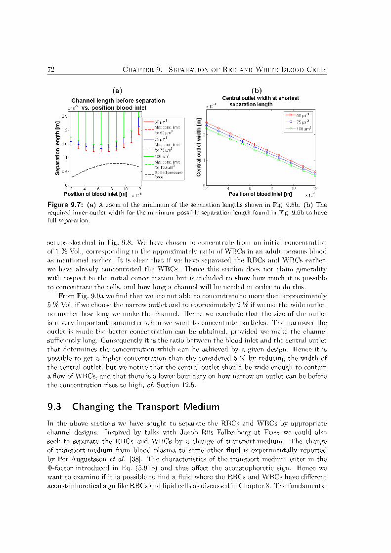
72 Chapter 9. Separation of Red and White Blood Cells
(a) (b)
Figure 9.7: (a) A zoom of the minimum of the separation lengths shown in Fig. 9.6b. (b) Therequired inner outlet width for the minimum possible separation length found in Fig. 9.6b to havefull separation.
setups sketched in Fig. 9.8. We have chosen to concentrate from an initial concentrationof 1 % Vol., corresponding to the approximately ratio of WBCs in an adult persons bloodas mentioned earlier. It is clear that if we have separated the RBCs and WBCs earlier,we have already concentrated the WBCs. Hence this section does not claim generalitywith respect to the initial concentration but is included to show how much it is possibleto concentrate the cells, and how long a channel will be needed in order to do this.
From Fig. 9.9a we find that we are not able to concentrate to more than approximately5 % Vol. if we choose the narrow outlet and to approximately 2 % if we use the wide outlet,no matter how long we make the channel. Hence we conclude that the size of the outletis a very important parameter when we want to concentrate particles. The narrower theoutlet is made the better concentration can be obtained, provided we make the channelsufficiently long. Consequently it is the ratio between the blood inlet and the central outletthat determines the concentration which can be achieved by a given design. Hence it ispossible to get a higher concentration than the considered 5 % by reducing the width ofthe central outlet, but we notice that the central outlet should be wide enough to containa flow of WBCs, and that there is a lower boundary on how narrow an outlet can be beforethe concentration rises to high, cf. Section 12.5.
9.3 Changing the Transport Medium
In the above sections we have sought to separate the RBCs and WBCs by appropriatechannel designs. Inspired by talks with Jacob Riis Folkenberg at Foss we could alsoseek to separate the RBCs and WBCs by a change of transport-medium. The changeof transport-medium from blood plasma to some other fluid is experimentally reportedby Per Augustsson et al. [38]. The characteristics of the transport medium enter in theΦ-factor introduced in Eq. (5.91b) and thus affect the acoustophoretic sign. Hence wewant to examine if it is possible to find a fluid where the RBCs and WBCs have differentacoustophoretical sign like RBCs and lipid cells as discussed in Chapter 8. The fundamental

Chapter 9. Separation of Red and White Blood Cells 73
(a) (b)
Figure 9.8: (a) Shows the one-inlet setup with center outlet of half the full channel width,w = 350 µm. (b) Shows a sketch of the one-inlet setup with a center outlet of width w/5 = 70 µm.
idea is previously used by F. Petersson et al. [30] to separate normally acoustical inseparableparticles by changing the density of the transport medium, and hence altering the pressureforce.
We start by considering the expression for the Φ-factor from Eq. (5.91b),
Φ =ρs + 2
3(ρs − ρ0)2ρs + ρ0
− 13c2aρ0
c2sρs. (9.1)
We see that it only depends on the fluid in ρ0 and ca. We are interested in the case wherethey have different signs, which means that sgn [Φred · Φwhite] = −1. We have indicatedthe values of ρ0 and ca, where this is the case in Fig. 9.9b. Notice that it is a very smallband of possible pairs of values. Furthermore the required speed of sound decreases withgrowing density, which is a problem because the speed of sound usually increases withgrowing density. However we were able to find one fluid that satisfied our requirements,namely nitrobenzene (C6H5NO2). The density of nitrobenzene is ρ0 = 1199 kg m−3, andthe speed of sound is ca = 1463 m s−1 [17]. With these values we find
Φred = 0.0053 and Φwhite = −0.0062. (9.2)
This shows that nitrobenzene has the exact property of making the WBCs moving to theedges of the channel and the RBCs moving towards the center. But the drawback is that itis highly toxic and possibly a carcinogen, which would make it dangerous to use in practice.Furthermore these calculations require accurate values for the compressibility and speedof sound of both the RBCs and WBCs.

74 Chapter 9. Separation of Red and White Blood Cells
(a) (b)
Figure 9.9: (a) Shows the concentration as a function of the channel length for the two setupsshown in Fig. 9.8. (b) The allowed values for ρ0 and ca where the acoustophoretic sign is differentfor RBCs and WBCs.
9.4 Summary
We have by numerical simulations analyzed different channel designs for separation ofparticles with Φ > 0, here with the example of RBCs and WBCs in blood plasma. Wefind that the WBCs are affected by a larger pressure force and that separation from RBCsof different sizes is obtainable in intervals of channel lengths. The larger the consideredRBCs, the larger is the effect of the pressure force, making it more difficult to separatethe RBCs from the WBCs. By varying the position of the blood inlet we have shown thatthe minimum separation length is obtained when the inlet is placed asymmetrically in thechannel a little towards the edge of the channel and not exactly where the pressure forceis largest. In this way all particles pass through the maximum of the pressure force.
Furthermore we have discussed concentration of the WBCs and shown that after chan-nel lengths of about 2− 5 cm, maximum concentration is obtained with the chosen outletsizes. In this context we have observed that the width of the outlet channel is a veryimportant design parameter when considering concentration the way it influences both themaximum achievable concentration and the length at which this occurs.
Finally we have discussed separation by varying the Φ-factors of the particles by usinganother transport medium. It is shown that it theoretically is possible to achieve differentacoustophoretic sign of RBCs and WBCs but in practice it would be difficult to find asuitable transport medium.

Chapter 10. Separation of Lipid Particles in Milk 75
Chapter 10
Separation of Lipid Particles in
Milk
Until now we have sought to separate particles with different compressibility, density, andsize. Inspired by Jacob Riis Folkenberg at the company Foss who works on separation oflipid particles in milk this chapter will focus on this separation.
Foss produces measurement equipment for the food industry. In this respect the fatparticles are mixed with cells present in the milk, thus hindering the analysis of these cellsby other means (often optical). Therefore it is interesting to be able to remove the fatfrom the milk, in such a way that the milk is not containing fat particles larger than acertain size. This ensures that the analyses sensitive to particle size (for instance scatteringeffects) are not influenced by the fat particles [1].
10.1 Design Considerations
We use the parameters for milk and fat particles found in Tables 7.2 and 7.3 resulting inthe fact that the fat particles are moving towards pressure anti-nodes (anti-nodes in thevelocity potential).
In practice when dealing with lipid particles in microchannels there is a tendency thatthe particles in the milk will stick to the sidewalls, according to [1]. This would be the casewhen using the above described channels with a width of λ/2. A way to avoid this is touse channels of width w = 3λ/2, where the lipid particles are injected in the middle partof the channel in an inlet not wider than w/3 centered around the middle of the channel.This means that the particles would move towards the two anti-nodes at w/3 and 2w/3.
Particles injected exactly at y = w/2 would according to the analytic solution, Eq. (6.3),never begin to move in the y-direction because the pressure force is exactly zero at thatpoint. However this would never be seen in practice since there would be some fluctuations(or other not yet understood processes) pushing the particle a little away from y = w/2leading to a non-zero pressure force on the particle. In our analysis we have to estimatethe effects of these fluctuations, and we do this by assuming that particles ate injected atleast a particle radius away from the middle of the channel.
Due to the symmetry of the problem we run our simulations in the region y = w/3

76 Chapter 10. Separation of Lipid Particles in Milk
(a) (b)
Figure 10.1: (a) Particle trajectories of particles injected in a inlet of width w/16 around thecenter of the channel (such that we only see half of the inlet channel in the plot). For each particlesize the trajectory of the inner- and outermost particle in the inlet channel is plotted. (b) Channelsetup for lipid particle separation. The idea is that at the inner outlet all particles above a diameterD0 should be near the dotted lines and flow through the outer outlet channels. These particleswill move faster towards the anti-nodes at w/3 and 2w/3 (green lines), which are values of y lyingin the outer outlet channels.
to y = w/2, where the results can be mirrored onto the other side of the channel. As inChapters 8 and 9 we are considering steady-state situations where it can be assumed thatthere are particles along all the single-particle trajectories.
A plot of the particle trajectories is seen in Fig. 10.1a where we use the dimensionsfrom Table 7.1. At first we focus on the problem of sorting all particles above a certaindiameter away from the milk. A setup for this sorting is shown in Fig. 10.1b. The purposeof the setup is to use that the velocity of a particle in the y-direction is proportional to thesquare of the particle radius, and thus the distance before a particle reaches an anti-nodedepends strongly on R, see Eq. (6.4).
To be sure that all particles with a diameter greater than D0 have moved away fromthe center outlet (where the milk exits) we must look at the trajectory of the innermostparticle which is the last particle of a given size to reach an anti-node. As an example weconsider three different channels where the center outlet width is set to 335 µm, 295 µm,and 255 µm, see Fig. 10.2. For each particle diameter we find the required length of thechannel before the particle exits in the outer outlet channel (which corresponds to theintersection between the trajectory and the black dashed line in Fig. 10.2a). These lengthsare given as a function of the particle diameter D0 in Fig. 10.2b. At a given length allparticles of a diameter larger than D0 must be in the outer outlet channels. We see thatthe required length does not depend very much on the center outlet width. This is becausethe velocity of the particles in the y-direction is large compared to the velocity in the x-direction. This leads to a range of y-values for which the trajectory curves are „flat” as seenin Fig. 10.2a. Thus the particles will move very quickly over a large part of the channel

Chapter 10. Separation of Lipid Particles in Milk 77
(a) (b)
Figure 10.2: (a) Particle trajectories of the innermost particles in the considered channel. Theblack dashed line must be understood as when the particles are to the left of this, they exit in anouter outlet channel. (b) Length of channel required for all particles of diameter D0 to be only inouter outlet channels.
making it less important where in the „flat” part of the trajectory the outlet change is.From Fig. 10.2b we conclude that it is possible to choose a length of the channel for sortinglarge particles away from the milk. If we for example want to remove all particles largerthan 3 µm from an inner outlet 295 µm wide we must use a channel with a length of ∼ 1cm.
Comments on the flat trajectory
Due to the flat trajectory, the particle can almost all the time be considered as lying eithernear the center of the channel or near the anti-node, where the anti-node in the λ/2-casewould be at the channel edge. This is because the shift from the center to the anti-nodehappens over a very short channel length, and thus making the device very sensible tovariations in channel lengths. In Section 6.2 we found that the travelled distance in the x-direction scales with 〈Eac〉−1. Because the acoustical energy density is difficult to determineexactly in a given channel in practice, there is an uncertainty in the theoretical predictionsof the required channel length to promote a certain separation. If we try to design andmake calculations on a setup where some of the particles are taken out somewhere inbetween the center and the anti-node, it would be difficult to determine the exact size ofthe particles that would flow out of that channel.
In an experimental setup we would be able to see separation in multiple outlet channelswhere the particles are sorted according to their size in the different channels with thelargest in the outermost channels as reported in [30]. The situation where the separationtakes place is found by tuning the applied voltage or by adjusting the flow velocity untilthe desired particle flows out of the various outlets. In our opinion it would be difficultto make good theory for this multiple separation system because of the uncertainty in theacoustical energy density, which experimentally is taken care of by tuning the parameters.But we find that it would be possible to make a reasonably estimate if a particle of a givensize is near the center or the edge of a channel for a given channel length. This we willconsider in the following.

78 Chapter 10. Separation of Lipid Particles in Milk
Figure 10.3: Comparison of numerical results with Eq. (10.1) with ys = w/3 + 40 µm corre-sponding to a center outlet width of 295 µm. It is seen that the analytical solution matches almostperfectly.
10.2 Analytical View on the Sorting
We see from Eq. (6.15) that the required length of the channel scales linearly with Δp/L(as the velocity in the x-direction scales linearly with Δp/L), so if we want to sort forother D0 than the channel was designed for, we just have to adjust the flow velocity.
Because of the flatness of the flow velocity profile in the x-direction, vx(y), around themiddle of the channel, see Fig. 8.6a, we are tempted to assume, that we can consider theflow velocity of the milk as constant here. In Section 8.6 we saw that the velocity wasconstant to four significant figures in the center third of the channel, so this is a reasonableassumption. According to Eq. (6.18), the required length of the channel when the particletravels from a position y to the position of the splitting point between the middle andouter outlet channel, ys, is:
x(y, ys) =3ηvx,av
4〈Eac〉k2yR
2Φlog(
tan(kyys)tan(kyy)
), (10.1)
where ky = 2π/λ = 3π/w and where y must be the position of the innermost particlewhere it enters the channel. This gives the minimum length of the channel to be surethat, according to our assumptions, all particles with radius R = D0/2 are not exitingthrough the center channel. That this analytic expression can be used instead of numericalsimulations is apparent from the plot of Eq. (10.1) together with the numerical solutiongiven in Fig. 10.3.
Knowing the geometry of the channel, we can easily regulate the average flow velocityaccording to Eq. (10.1) thus avoiding the need for numerical calculations in order to beable to sort particles of a given size from a sample.
As another interesting example of particle sorting, though not very viable for the appli-cation of removing all large fat particles from the milk, we will also discuss another sortingopportunity this setup can provide. Consider the case where we only want to have particles

Chapter 10. Separation of Lipid Particles in Milk 79
(a) (b)
Figure 10.4: (a) Particle trajectories of the outermost particles in the considered channel. Theblack dashed line must be understood as when the particles are left of this, they exit in an outeroutlet channel. To the right of the dashed line they exit through a central outlet of the width295 µm. (b) Length of channel required for no particles of diameter below D0 to leave the outeroutlet channels.
above a certain radius in the outer outlets. Since this is not directly linked to removing allparticles above a certain threshold, we will only consider this case from an analytical pointof view, where Eq. (10.1) also is applicable. To be sure that no particles with a diametersmaller than D0 enters the outlet channels, we have to consider the outermost particlesin the inlet channel. The trajectories of these particles are given in Fig. 10.4a and thecorresponding plot for the diameters is given in Fig. 10.4b. We see that it is possible todesign a channel where the particles in the outer outlets are only above a certain diameter.For example if we want to make sure that no particles with a diameter below D0 < 4 µmis entering through the outer outlets, when the central outlet is 295 µm, we can have amaximum channel length of 2.5 mm.
10.3 An Idea for Milk Separation in Practice
In this section we want to describe a way that lipid separation in milk could be donein practice. The channel setup is shown in Fig. 10.5, and the basic idea is to use the3λ/2-channel as described above for the separation remembering that lipid particles havea negative acoustical sign. We require that the particles enter the 3λ/2-channel in a smallinterval around the middle of the channel to optimize the separation. A way to make thisfocusing is to let the particles enter in the middle of a channel of width 2λ/2, long enoughfor the pressure force to be able to focus a particle beam in the middle of the channel. Thelipid particles will be focused in the middle due to the anti-node at the center.
An experimental procedure for separation would be first to determine the acousticenergy in the channel, then calculate the required length of the channel to separate certainparticles from Eq. (10.1) with a given flow rate, and at last do the separation of the desiredparticles in the channel.
A way to estimate the acoustical energy could be to use a test-fluid with known viscosity

80 Chapter 10. Separation of Lipid Particles in Milk
Figure 10.5: System for separation of particles with Φ < 0. The particles are focused in a beamin an area of width w = 2λ/2 and are afterwards separated in a channel of width w = 3λ/2.
and test particles with known Φ-factor and radius. One have to inject the test-fluid intothe channel and then have to adjust the flow velocity to find the flow velocity where theparticles change from exiting through the inner outlet to exiting from the outer outlet orvice versa. This value together with the channel length can be inserted in Eq. (10.1) tofind an expression for 〈Eac〉. In the equation y would be the outermost point of the focusedparticle beam entering the 3λ/2-area, and ys would be the y-coordinate of the splittingpoint between the center and outer outlet channels.
There are uncertainties related to this process of determining the acoustic energies.For example we are not certain how the particles are affected at the interface betweentransport-medium and buffer-medium which would require further investigations beyondthe scope of this thesis. By choosing a buffer-medium with viscosities close to the one ofmilk, we might be able to minimize these effects. Similar viscosities in buffer and milkwould also strengthen the assumption of a constant flow profile in the middle region of thechannel (according to Section 12.2). If the same flow velocity in the fluid inlets is usedwe will avoid any questions about how laminar flows with different velocities affect eachother.
10.4 Summary
We have by numerical analyses suggested a design and procedure for separation of Φ < 0particles with the example of lipid particles in milk, where we were able to sort largeparticles away from the milk. We have seen that by only operating in the 1/3-central partof a 3λ/2-channel with the same viscosity in the whole channel, we can approximate theflow velocity profile with a constant average velocity. This leads to a simple analyticalsolution which describes the separation length from which we with well-known particlesare able to determine the average acoustical energy density in the channel. One could trytheoretically to estimate how precisely we are able to split the particles in size, but a lotof experimental factors influence on this.

Chapter 11. Other Possible Applications of the Pressure Force 81
Chapter 11
Other Possible Applications of the
Pressure Force
In this chapter we will present other possible applications of the pressure force, besideswhat we have learned that other research groups have worked with.
11.1 Size-sorting of Particles with Φ > 0
The principle of sorting similar particles with Φ > 0 is like the situation with Φ < 0illustrated by the separation of fat-particles in milk, cf. Chapter 10, but we have to designthe channel in another way because the particles now move towards nodes and not anti-nodes of the pressure field, see Section 5.6. A setup with this functionality is shown inFig. 11.1a where the particles first are focused in two beams in a 2λ/2-channel. These twobeams function as inlets for a succeeding λ/2-channel. In this way the situation in the λ/2-channel is similar to the WBWBW-system for blood we have discussed in Section 8.6 forthe purpose of separation of RBCs and lipid particles. In the setup sketched in Fig. 11.1awe would just have a higher concentration of RBCs in the inlet channels than we wouldhave if we had inlets of „regular” blood which had not been concentrated. Therefore thissystem would be good for optimizing the blood separation setup where we both have highthroughput and short channel lengths. Furthermore it is convenient to have the sameviscosity in the channel, as we would have using this system, according to the discussionon velocity flow profile in Section 12.2.
The experimental procedure is the same as for milk, as we described in Section 10.3,where a known test-particle is used to determine the acoustical energy density for calcu-lating the required flow velocity by Eq. (10.1).
11.2 Creation of Pulses of Particles
For practical microfluidic applications it could be useful to be able to have particles arrivingin a pulses. We illustrate a channel for particles with Φ < 0, and a similar system couldbe made for particles with Φ > 0.

82 Chapter 11. Other Possible Applications of the Pressure Force
(a) (b)
Figure 11.1: (a) Setup for size-sorting of particles with Φ > 0. First a channel of width 2λ/2focuses the particles into two beams at the pressure nodes. These beams are by a laminar flow ledinto a channel of width λ/2 in such a way that the two beams lie near the edge of this channel.This is done by leading some of the fluid out from the 2λ/2-part in some outer outlet channels asillustrated. In the λ/2-part the particles are focused into the center of the channel. (b) Setup tocreate pulses for particles with Φ < 0. The piezo-actuator is periodically turned on an off causingthe particles to be periodically sent either into the inner or the outer outlet(s). Note that thepressure force is assumed large compared to the flow velocity such that when the actuator is on,the particles move very fast to the edge. The dashed lines outline the flow profile when the actuatoris turned off.
The pressure force could be used to create pulses by turning on and off the piezo-actuator (or at least varying the frequency between the resonance frequency and off-resonance frequency), for the channel setup in Fig. 11.1b. The particles are injected inthe center inlet of a WBW-system in a λ/2-channel of length L (this situation could alsobe achieved by focusing of the beam in a 2λ/2-channel as described in Fig. 10.5). Weassume that the pressure force on the particles, when the actuator is turned on, is so large,that the traversed length in the x-direction before the particle is at a y-position, where itwould exit through the outer outlet channel, x(y1, y2), is very small compared to L. Thismeans that when the actuator is switched on, almost all particles in the channel at thattime will flow out of the outer outlets.
We assume that the velocity in the center of the channel is vx, and that the actuatoris switched on in a time interval ton. It gives a total length of a pulse of, ` ≈ L + vxton— including the contribution both from the particles in the channel when the actuatoris turned on and the particles entering the channel while the actuator is turned on also

Chapter 11. Other Possible Applications of the Pressure Force 83
contribute to the length of the pulse. From these assumptions we also see that the timebetween the piezo is turned off until it can be turned back on again must be toff > L/vx.Because the pulse length with this simple model is ` > L, a period of switching the actuatoron and off is T = ton + toff, which must be equivalent to T = `/vx + Δt, where Δt is thetime between the pulses.
To get an estimate of the pulse frequency we can obtain, we assume that the timebetween pulses is the same as the time we experience a pulse, i.e. Δt = `/vx. This givesa period of T = 2`/vx corresponding to a frequency of f = vx/(2`) < vx/(2L), limited bythe length of the channel and the flow velocity. Using standard parameters vx = 0.1 m/sand L = 5 mm, we find f < 10 Hz.
The frequency can be made larger and the pulses smaller by looking at exactly howlong time a particle entering in the middle of the channel uses to get to a point where itwould flow out of an outer outlet channel. For optimization, analysis like in Chapter 8could be made, but it is beyond the scope of this thesis.

84 Chapter 11. Other Possible Applications of the Pressure Force

Part III
Neglected Effects
85

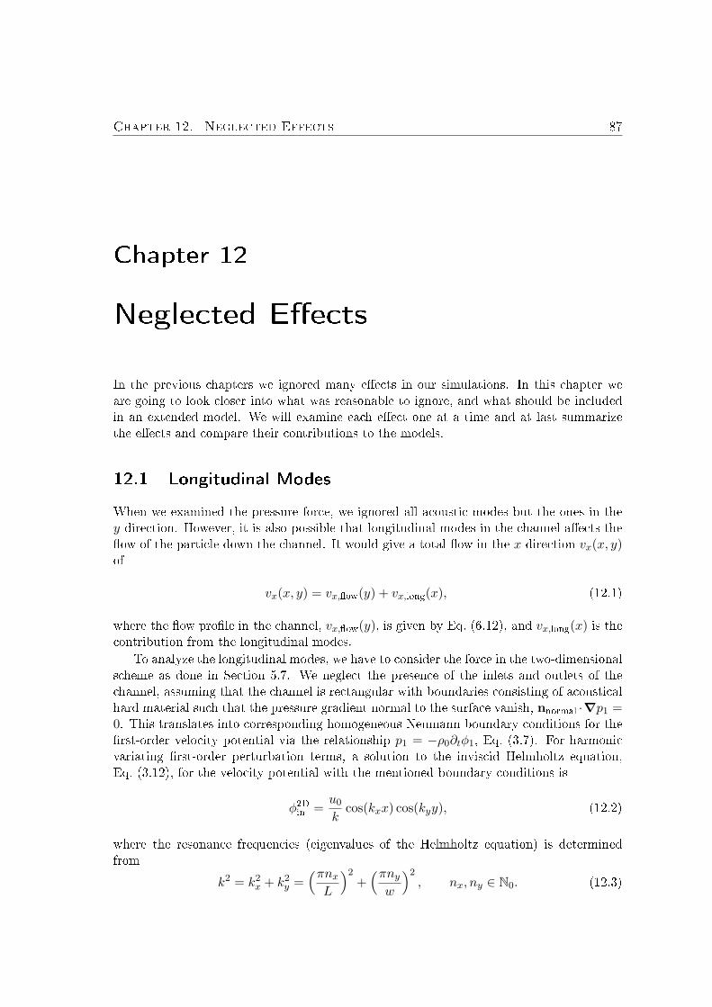
Chapter 12. Neglected Effects 87
Chapter 12
Neglected Effects
In the previous chapters we ignored many effects in our simulations. In this chapter weare going to look closer into what was reasonable to ignore, and what should be includedin an extended model. We will examine each effect one at a time and at last summarizethe effects and compare their contributions to the models.
12.1 Longitudinal Modes
When we examined the pressure force, we ignored all acoustic modes but the ones in they-direction. However, it is also possible that longitudinal modes in the channel affects theflow of the particle down the channel. It would give a total flow in the x-direction vx(x, y)of
vx(x, y) = vx,flow(y) + vx,long(x), (12.1)
where the flow profile in the channel, vx,flow(y), is given by Eq. (6.12), and vx,long(x) is thecontribution from the longitudinal modes.
To analyze the longitudinal modes, we have to consider the force in the two-dimensionalscheme as done in Section 5.7. We neglect the presence of the inlets and outlets of thechannel, assuming that the channel is rectangular with boundaries consisting of acousticalhard material such that the pressure gradient normal to the surface vanish, nnormal ·∇p1 =0. This translates into corresponding homogeneous Neumann boundary conditions for thefirst-order velocity potential via the relationship p1 = −ρ0∂tφ1, Eq. (3.7). For harmonicvariating first-order perturbation terms, a solution to the inviscid Helmholtz equation,Eq. (3.12), for the velocity potential with the mentioned boundary conditions is
φ2Din =u0
kcos(kxx) cos(kyy), (12.2)
where the resonance frequencies (eigenvalues of the Helmholtz equation) is determinedfrom
k2 = k2x + k2
y =(πnxL
)2+(πnyw
)2, nx, ny ∈ N0. (12.3)

88 Chapter 12. Neglected Effects
(a) (b)
Figure 12.1: (a) Contour plot of the normalized acoustic potential U2D/U0 in the case of nolongitudinal modes, kx = 0 and λ/2 = w, in a channel with w = 350 µm and L = 3 cm.Furthermore a RBC trajectory in blood starting near the channel edge is indicated. (b) Contourof the normalized acoustic potential U2D/U0 in the case of ky = 0 and nx = 3. Parameter valuesfor (a) and (b) are given in Chapter 7. Note that the axis are not equal.
In Section 5.7 we found that the harmonic velocity potential Eq. (12.2) leads to an acousticpotential, Eq. (5.95), given by
U2D = U0
[2f1 cos2(kxx) cos2(kyy)
− 3(k2x
k2sin2(kxx) cos2(kyy) +
k2y
k2cos2(kxx) sin2(kyy)
)f2
],
(12.4)
where U0 = (1/2)(4πR3/3)〈Eac〉 has been introduced as a natural energy scale for theacoustic potential.
Below we choose to make analyses of a system as the one indicated for blood separationin Chapter 7 with w = 350 µm, and with a channel length L = 3 cm as used as a typicallength for separation of particles in practice [30].
In Part II we have only been considering the special case where kx = 0. In Fig. 12.1a aplot of the potential together with a particle trajectory for a RBC in blood is seen wheref = 2.119 MHz and ny = 1, corresponding to only having one node in the y-direction. Wesee that the acoustic potential is invariant in the x-direction, which also can be seen fromEq. (12.4) with kx = 0.
Considering the ky = 0 mode
The opposite situation with no modes in the y-direction, ky = 0, is shown in Fig. 12.1b andhas f = 0.742 MHz. We notice that the pressure force in this situation is only affectingthe particles in the x-direction. In the x-direction the particles already have the velocityvx,flow due to the flow profile in the channel. Hence the pressure force will either counteractor amplify the flow velocity depending on the x-position of the particle. We see that the

Chapter 12. Neglected Effects 89
magnitude of the pressure force in this setup in analogy of the case with kx = 0 where〈Fx〉 = 4πkxR3〈Eac〉Φ sin(2kxx). In equilibrium this force is balanced by the Stokes drag,Fx,drag = 6πηRv, giving a maximum contribution from the longitudinal modes of
|vx,long| =23ηkxR
2〈Eac〉Φ =2πnx3Lη
R2〈Eac〉Φ, nx ∈ N0. (12.5)
This must according to Eq. (12.1) be compared with the magnitude of the velocity flowprofile to determine which of the velocities that gives the major contribution to vx(x, y).
Using typical values as given in Chapter 7 for the blood simulations, we estimate thedrag velocity in the channel with L = 3 cm to have the magnitude |vx,long| ≈·0.27 mm s−1
for the mode nx = 10. This must be compared with the average magnitude of the flowprofile of vx,flow = 0.11 m s−1, and thus the longitudinal modes on the whole do not changethe flow in the x-direction in this considered case.
If the flow velocity in the flow profile is comparable but still larger than the velocitycontribution from the longitudinal mode, the particles will move in the x-direction peri-odically slowing down and speeding up according to the sine variation of the longitudinalmodes from the pressure force. On the other hand if the velocity in the x-direction fromthe flow profile is smaller than the magnitude of the longitudinal contribution, the particleswill collect at the nodes (for Φ > 0) in the acoustic potential. At a threshold flow velocityv∗x,flow, the flow velocity exactly balances the velocity from the pressure force in a givenmode,
v∗x,flow = |vx,long| =2πnx3Lη
R2〈Eac〉Φ, nx = N0. (12.6)
From this we can experimentally determine an estimate of 〈Eac〉 in a given channel usingthe threshold flow velocity as suggested in [6].
The Maximum Magnitude of the Longitudinal Velocity Contribution
When looking at the maximal velocity contribution from the longitudinal modes, we con-sider the the pressure force in the x-direction for arbitrary wavenumbers, Eq. (5.98),
〈Fx〉 = U0kx sin(2kxx)
[2f1 cos2(kyy) + 3f2
(cos2(kyy)−
k2y
k2
)], (12.7)
〈Fx〉 ≤ U0kx
[2|f1|+ 3|f2|
], (12.8)
which is equal to the magnitude of the one-dimensional force, where ky = 0, as seen bycomparison with Eq. (5.89c). Hence we conclude that the estimate of the magnitude ofthe longitudinal velocity contribution made above in the case of ky = 0 is in fact also anestimate of the maximum magnitude of the longitudinal velocity contribution in 2D. Itshould be noted that the maximum magnitude is proportional to the mode number, so forvery high order of modes or small velocity profiles the velocity originating from the modescan have influence.

90 Chapter 12. Neglected Effects
(a) (b)
Figure 12.2: (a) Contour plot of the normalized acoustic potential U2D/U0 with ny = 1 andnx = 1. (b) Contour plot of the normalized acoustic potential U2D/U0 with ny = 1 and nx = 3.In both (a) and (b) we see the trajectories of RBCs experiencing the shown potential (solid blackline), a potential corresponding to kx = 0 (dashed black line) and a potential corresponding to halfthe force from a kx = 0 field (dashed white line) are plotted.
Considering Longitudinal Modes with one Transverse Mode
Even though the pressure force in the x-direction is very small compared to the flow velocityprofile, the longitudinal modes introduce changes overall in the potential field. Hence thepotential in the y-direction is changed and it thus alters the trajectory of a particle. Wewill in the following investigate this effect in our standard configuration for blood with onenode in the y-direction, corresponding to ny = 1 or as previously denoted w = λ/2, andlook at multiple nodes in the x-direction.
First of all we consider a situation with only a few nodes in the x-direction. The acousticpotential for nx = 1 and nx = 3 is seen in Fig. 12.2 together with trajectories for a RBCin blood. The modes have frequencies of fnx=1 = 2.119 MHz and fnx=3 = 2.120 MHzfrom Eq. (12.3). As the second thing we consider the case of nx = 25, corresponding toa frequency of f = 2.207 MHz shown in Fig. 12.3a. We see that the longitudinal modesintroduce periodic plateaus in the y-direction, corresponding to the minima in the potential,where particles are not affected by the pressure force in the y-direction. Due to the flowvelocity profil the particles move forward in the x-direction even in areas without pressureforce. Hence this mode setup cannot prevent the particles with Φ > 0 from following theflow in the x-direction as we could for ky = 0, because the potential has a minimum inthe center of the channel. Eventually the Φ > 0 particles will collect at the center andexperience no pressure force and just follow the flow in the x-direction.
When considering a case with nx = 25, see Fig. 12.3a, the potential qualitatively looksa lot like that with kx = 0, but it is seen that that the trajectories in these two cases differa lot. We thus search for a explanation of this behaivour in the following.

Chapter 12. Neglected Effects 91
(a) (b)
Figure 12.3: (a) Contour plot of the normalized acoustic potential U2D/U0 with ny = 1 andnx = 25. The trajectories of RBCs experiencing the shown potential (solid black line), a potentialcorresponding to kx = 0 (dashed black line) and a potential corresponding to half the force from akx = 0 field (dashed white line) are plotted. (b) Contour plot of the normalized acoustic potentialU2D/U0 with ny = 1 and nx = 3. The trajectories of RBCs experiencing the shown potential(solid black line) and a potential corresponding to half the force from a kx = 0 field (dashedwhite line) are plotted. The trajectory marked 1 is for an average flow velocity of 2vx,flow, 2 is forvx,flow = 0.11 m s−1, and 3 is for 1/2vx,flow.
The Average Force Exerted
When considering the introduced periodicity in the x-direction, it is natural to average thepressure force experienced by the particle over the period in the acoustic potential, Tx, inthe x-direction, Tx = 2π/kx. It is reasonably to consider the particle trajectory by theaverage over the spatial coordinate x, if the change in the potential/force which a particleexperiences varies on a much shorter length scale in the x-direction than in the y-direction.The characteristic time scale of the potential change is the time it takes for a particle tomove one period in the given direction, Δt. If the characteristic velocity in the x-directionis denoted vx, and one period in the x-direction has a length of the order L/nx, the timeit takes for the potential to change notably is of the order Δtx ∼ L/(nxvx). Similarlythe change in y-direction is of the order Δty ∼ w/(nyvy). Hence we must require for theaverage to be in good agreement with the actual particle trajectory that
Δtx � Δty ⇔nywvy �
nxLvx. (12.9)
This should be understood such that the nodes passed per time by the particle must belarger in the x-direction than in the y-direction. It ensure that it is possible to consider they-coordinate as constant while we experience a notably change the x-coordinate. Hencethe larger number of modes per length or the bigger the characteristic velocity in thex-direction, the better we can expect an average to describe the particle trajectory.
The characteristic velocity in the x-direction is the velocity from the flow profile. Inthe systems discussed in part II we are considering flow velocities of the order vx,flow ≈0.11 m/s. The characteristic velocity in the y-direction is the velocity originating from the

92 Chapter 12. Neglected Effects
pressure force in the y-direction. This can be estimated in the same way as done in thex-direction for the case ky = 0 in Eq. (12.5). Using typical values for RBCs we estimatevy,long = 2.3 mm s−1. Therefore we fulfill the condition for the average to be close to theparticle trajectory in the considered setup.
Thus it is valid to use the spatial average of 〈Eac〉 in the x-direction, and from Eq. (5.98)we find
〈Fx〉 = U0kx sin(2kxx)
[2f1 cos2(kyy) + 3f2
(cos2(kyy)−
k2y
k2
)], (12.10a)
〈Fy〉 = U0ky sin(2kyy)[2f1 cos2(kxx) + 3f2
(cos2(kxx)−
k2x
k2
)], (12.10b)
leading to
〈Fx,average〉 = 0. (12.10c)
〈Fy,average〉 =12U0ky sin(2kyy)
[2f1 + 3f2
(1− 2
k2x
k2
)](12.10d)
=12〈Fy,kx=0〉 − 3f2U0ky sin(2kyy)
k2x
k2. (12.10e)
The last equality follows from comparison with the expression for the one-dimensional forceEq. (5.91a). This shows that the average force exerted on the particles is half the forcefrom a potential field with kx = 0 but including an extra term with the same sine-variationas the pressure force in the y-direction. Thus the deviation from the (1/2)〈Fy,kx=0〉 effectis biggest when the pressure force in the y-direction is largest, hence when the velocity inthe y-direction is largest.
Comparison with the Potential Without Longitudinal Modes
When considering the average force in Eq. (12.10c) we notice that it corresponds to half theforce exerted from a potential than in the situation with kx = 0 when the term 2k2
x/k2 ≈ 0.
This is the case when
k2x
k2x + k2
y
� 1 ⇔ 1
1 +(nyLwnx
)2 � 1 ⇔ nyw� nx
L. (12.11)
This means that when the nodes per length is greater in the y-direction than in the x-direction, the average force exerted from a mode with nx 6= 0 corresponds to (1/2)〈Fy,kx=0〉.For the considered channel setup we have ny/w = 1/w = 2.9 × 10³ m−1 and nx/L =100 m−1 for nx = 3, thus fulfilling Eq. (12.11).
In Figs. 12.2 and 12.3 the trajectory of a RBC is plotted in different potentials togetherwith the trajectory for a similar RBC affected by 1
2〈Fy,kx=0〉. Furthermore the trajectory ofa particle experiencing the one-dimensional pressure force is calculated for comparison. Wenotice the great agreement between the actual trajectory and the (1/2)〈Fy,kx=0〉 trajectoryas predicted by our theory.

Chapter 12. Neglected Effects 93
(a) (b)
Figure 12.4: (a) A cross-section of the Pouseille-flow in a BWB-channel with different viscosities,respectively blood and water. The velocities are given in m s−1. (b) A cross-section of thePouseille-flow in a BWB-channel with constant viscosity. Notice that vx is measured in m s−1.
In Fig. 12.3b we have furthermore shown the proposed dependency on the flow velocityEq. (12.9), when plotting the trajectories of RBCs in a nx = 3 potential for differentflow velocities in the x-direction. We find that the case with the highest flow velocityhas the best agreement between the actual particle trajectory and the particle affectedby (1/2)〈Fy,kx=0〉, showing that the averaging approximation is best when operating withlarge flow velocities, which confirms Eq. (12.9).
We conclude that if the flow velocities compared to the nodes per length in the twodirections fulfill Eq. (12.9), and we furthermore have the dimensions of the channel fulfillingEq. (12.11), the particle trajectory in the actual potential can very well be approximatedby the trajectory of a particle affected by (1/2)〈Fy,kx=0〉.
12.2 The Influence of the Viscosity on the Pouseille-flow
An effect we have neglected in our analysis of the separation of RBCs from lipids or WBCsis that the viscosity of the buffer medium is not necessarily the same as that of the transportmedium. For blood we have used that η = 0.0027 Pa s. However the viscosity of water,which is a reasonable approximation for what could be used as buffer medium, at 20◦Cis 0.0010 Pa s [5]. The differential equation for the Pouseille flow in each medium can bederived from the Navier–Stokes equation, since η only varies at the boundaries between twoflows so it can be assumed constant in each medium. Whe notice that a steady-state flow ina channel which is translational invariant in the x-direction, cannot depend the x position.Furthermore the flow velocity can only have an x-component. Hence the velocity in eachmedium must have the form v(y, z) = vx(y, x)ex. With a steady-state velocity of thisform we see from the Navier–Stokes equation that the velocity must fulfill the differentialequation, [5],
− η[∂2y + ∂2
z
]vx(y, z) =
ΔpL. (12.12)

94 Chapter 12. Neglected Effects
(a) (b)
Figure 12.5: (a) A comparison of the flow-speeds in the middle of the channel for the twodifferent models using the viscosity of water and blood respectively. The two vertical lines showthe splitting of the three inlets. (b) The ratio of vx found using the model with different viscositiesto the vx found using constant viscosity.
The boundary condition at the edges of the channel is that vx goes to zero. At the interfacebetween the two flows we have that the shear stress is constant, and since the shear stressis given as σ = η∇v, we get
η1∇vx,1 = η2∇vx,2. (12.13)
where the indices refer to the different media. We have implemented Eqs. (12.12) and (12.13)in Comsol with the three-channel BWB-system described in Section 8.4 where we are as-suming that the interfaces between the media are flat. In the optimal separation setup wehad blood in the interval [0 µm; 125 µm] and [225 µm; 350 µm] and buffer in-between.
A cross-section of the velocity-field with different viscosities in the channel can be seenin Fig. 12.4a. We have also simulated the flow with constant η = 0.0027 Pa s which canbe seen in Fig. 12.4b. Notice that there is a clear difference in the flow-type. The speedchanges a lot in the middle of the channel when having different viscosities.
We have plotted a cross-sectional view of vx at z = h/2 to compare the results forthe two models in Fig. 12.5a. We see that the biggest difference between the two modelsappears in the middle of the channel.
Furthermore we have plotted the ratio between the two flow-speeds, see Fig. 12.5b.From this figure we deduce that the conclusion from the RBC–lipid section not will bechanged dramatically, since it was the lipids that were the limiting factor, and they willnot move into the middle subdomain where vx is much larger. However we still see thatthe innermost lipids in the blood inlet (and RBCs for that sake) move almost 50 % fasterin the center when using the more sophisticated model than assuming the same viscosityin the buffer- and transport-medium.

Chapter 12. Neglected Effects 95
(a) (b)
Figure 12.6: (a) The Fåhraeus effect. Plot of the relative haematocrit Hct/Hc vs. the tubediameter D. (b) The Fåhraeus–Lindqvist effect. Plot of the apparent viscosity in the tube, ηapp,against the tube diameter D. More advanced models of the non-Newtonian behavior is given in[18] and gives small deviations (up to 0.15 in ηapp) from the simple model, but the tendency is stillthe same.
12.3 The Fåhraeus effect and Fåhraeus–Lindqvist effect
Two of the most relevant non-linear effects which are observed in blood flowing in smalltubes are according to [18] the Fåhraeus effect and the Fåhraeus–Lindqvist effect. Withoutgoing into details with the models behind these two effects we will just state the conse-quences. Note that the models are for straight, circular channels with diameter D wherewe in our work use rectangular cross-sections, but we assume that the same effects arepresent in rectangular channels.
The standard haematocrit is denoted Hc when the blood is in a large reservoir. TheFåhraeus-effect predicts a decrease in the concentration of RBCs, described by the dynamichaematocrit Hct, i.e. the apparent haematocrit value in the tube, when the diameter ofthe tube is reduced. The altered haematocrit values is due to the formation of a depletedplasma layer at the channel edges. The layer is formed because of migration of cells fromthe channel walls (where the migration has a higher flow velocity than the axial flowvelocity). Thus the Fåhraeus effect can be reduced by increasing the flow velocity, vx.
An empirical parametric description of the Fåhraeus effect is given in [23], and thisis plotted in Fig. 12.6a. The parameters used for the plot are unspecified, but it gives aqualitative but not quantiative description of the Fåhraeus effect.
The Fåhraeus–Lindqvist effect states a decrease in the apparent viscosity in the tube,ηapp, when the tube diameter is reduced. Due to stress-induced cell migration from theFåhraeus effect a slippage layer of plasma-rich, cell-depleted fluid appears near the tubewalls in small tubes, D = 5 µm − 0.3 mm [18]. The thickness of the layer depends of theflow rate and the tube diameter, but is experimentally shown more or less to remain inthe range 2 − 4 µm for all tube diameters [7]. Thus the relative volume of the plasmalayer (with low viscosity due to the Fåhraeus effect) to the tube volume is increased withdecreasing tube diameter. This effect is describe as the Fåhraeus–Lindqvist effect. Asimple model is given in [25] and plotted in Fig. 12.6b to give a qualitative impression of

96 Chapter 12. Neglected Effects
the Fåhraeus–Lindqvist effect. We see that the effect can change the viscosity significantlywhen having flow in small channels. But as noted in Section 6.2 the value of the viscositydoes not affect the particle trajectories in the channel, x(y), but only the time profiles, y(t)and x(t). Hence we conclude that this effect is not that important to our determinition ofthe channel length.
The Fåhraeus–Lindqvist effect as described above is valid for a haematocrit value upto 95 % [10]. When the haematocrit is higher, we will have a high dense packing of theRBCs which contributes to the non-Newtonian behavior of the fluid. Further discussionson the non-Newtonian behavior of blood and the effect of having a blood flow in channels(such as cell screening and plasma skimming) are described in detail in [18].
12.4 Temperature Dependence
Many of our parameters used in the simulations depend on the temperature. In this sectionwe will look closer at what this means for our results.
First we will look at the viscosity. According to [8] the viscosity of blood decreaseswith temperature, for values see Appendix F. Generally the viscosity of blood increaseswith approximately 2 % with a one degree decrease in temperature, see [8]. However asdiscussed in Section 6.2 this will not change the required travel lengths but only the timeto get there, and since we assume that we are in steady-state, this dependence can beneglected. However if we were to use a buffer medium at 20◦C and blood at 37◦C, thecooling and heating of the two fluids would change the relative viscosity between themthus leading to a different Pouseille-flow as discussed in Section 12.2, and this would bevery difficult to model.
We also know that the density and speed of sound in fluids change with temperature.From [17] we found values for the speed of sound versus temperature in water in 10◦Cincrements given in Appendix F. Regarding the density we found the following expression1
ρ =ρat τ0
1 + a0 (τ − τ0), where a0, water = 0.88× 10⁻⁴ ◦C−1, (12.14)
where τ is the temperature and τ0 is a reference temperature. Using that the densityof water at τ0 = 4 ◦C is ρ0 = 1000 kg m−3, we can find the Φ-factors as a function oftemperature, where we neglect the change in density and temperature of the particles inour fluid.
Using the above results for water Fig. 12.7a shows the change in Φ-factors versustemperature using water as our buffer medium. Notice that the values are scaled to theΦ-factor at 20 ◦C. In the simulations made in part II we used blood and milk as transportmediums, but we were not able to find the temperature dependence of the density and speedof sound for those two parameters. To see if running the system at different temperatureswould make it easier to separate our particles, we plot the ratio of the Φ-factor of RBCsto lipid and to WBCs in Fig. 12.7b, taking the absolute value of the RBC to lipid ratiofor clarity. We see that the ratio for RBCs–WBCs is almost independent of temperature,however it seems like we could improve our results for RBC to lipid separation. We stress
1http://www.engineeringtoolbox.com/fluid-density-temperature-pressure-d_309.html

Chapter 12. Neglected Effects 97
(a) (b)
Figure 12.7: (a) The ratio of the Φ-factors to Φ at 20 ◦C as a function of temperature. Noticethat these φ-factors are found with water as medium compared to the blood and milk we used inour simulations (b) The ratio of the Φ-factors as a function of temperature. Notice that we havetaken the absolute value of the RBC/lipid ratio for clarity.
that the temperature dependence of density and speed of sound for the particles is notincluded in the prior discussions. Furthermore as seen in Fig. 12.7a the Φ-factor for lipidparticles decreases with decreasing temperature which would mean that it would require alonger channel to separate the particles, as we discussed in Chapter 8. Still the temperaturedependence is something that could be looked deeper into, since it could possibly makethe separation easier.
12.5 Effects of Concentration
In the previous discussion we only considered single point-like particles. This is not thecase in reality where RBCs, WBCs, and lipids have a finite extension. Furthermore wehave multiple particles. This means that there is a maximum of the concentration in ourchannels. To simplify the analysis we will assume non-compressible spherical particles andcylinders.
To derive an expression for the concentration in our outlets as a function of the inletconcentration we consider N/Δt particles flowing in a channel per time. Thus Nin/Δt andNout/Δt particles are entering and leaving the channel respectively. We define Γ as thepercentage of particles from the inlet leaving in a desired outlet. The width of the streamis w. Since we assume that we have reached steady-state, we have for a time step Δt
Nout
Δt=
ΓNin
Δt. (12.15)
Using that N = cV we get
coutVoutΔt
=ΓcinVin
Δt⇔ coutwoutΔLout · h
Δt=
ΓwinΔLin · hΔt
, (12.16)
where we have used that the volume entering the channel during the time step Δt can beexpressed as winhΔLin and similarly the volume leaving the channel as wouthΔLout, where

98 Chapter 12. Neglected Effects
h is the height of the channel. ΔLin and ΔLout are the length of the volume element andcan be expressed by the velocity of the fluid in the channel as ΔL = vxΔt. By assuminga time-independent flow profile in the channel, we get
cout = cinwin
woutΓvoutvin
= Γ · cin ·win
wout(12.17)
This equation allows us to find the smallest possible proportion of the width of the out-let channel compared to the inlet because there are a physical maximum value for cout.According to the Kepler conjecture, the highest average density in a regular lattice arrange-ment of spheres is approximately cmax = 74 Vol%. This can be achieved with hexagonalclose-packed or face centered cubic structure.
However since the red blood cells are not spherical but rather toroidal shaped one couldimagine a stacking of cylinders instead of spheres. In this case the closest packing would beparallel cylinders placed in a hexagonal grid. Thus the maximum concentration becomescmax ≈ 91 %, which is significantly higher than for stacking of spheres.
Assuming that we are examining male blood with a haematocrit value of 46 Vol% [20],we are now able to find the smallest possible outlet channel assuming all the RBCs havemoved into the outlet channel, i.e. Γ = 1. Using Eq. (12.17) we arrive at
cout ≤ cmax = 1 · cin ·win
wout⇔ wout
win=
cincout≥ cincmax
=0.460.74
= 0.62, (12.18)
using spherical stackings. Thus the outlet channel has to be at least 62 % of the inletchannel if we want to have all the RBCs contained in it. However this value is a conservativeestimate since we have neglected compressibility, and the fact that the RBCs are notspherical. If we use the results for stacking of cylinders, we get that the outlet channelshould be at least 50 % of the inlet channel, still neglecting the compressibility of theRBCs.
This shows that we have to be careful not to choose too small an outlet channel for theRBCs if we want the calculations from the single-particle approach to be valid. We havenot considered the lipids since the concentration is considerable smaller [2], but the sameargument applies for them as well.
12.6 Diffusion
In this section we consider the many-particle effect connected with the diffusion of particleswhen there is a gradient in the concentration present. According to [5] the diffusion forcein a weak solution (low concentration) is given by
Fdiff = −∇µ, µ(T, ρ) = µ0 + kBT ln(ρ/ρ0), (12.19)
where µ(T, ρ) is the chemical potential, and where the subscript 0 refers to some constantstandard concentration. This leads to an expression for the size of the diffusion force inthe y-direction given as
Fdiff = kBT∂yρ
ρ= kBT
∂yc
c. (12.20)

Chapter 12. Neglected Effects 99
In Section 5.5 we have shown, that the acoustical force drives the RBCs towards the middleof the channel. According to Eq. (12.20) this leads to a diffusion force counteracting theacoustical force Eq. (5.91c). In steady-state when the particles do not move, the size ofthe two forces must be equal,
kBT∂yc
c= 4πkyR3〈EacΦ〉 sin
(2πny
y
w
), (12.21)
where ky = πny/w. Solving this differential equation for the first mode, ny = 1, gives
c(y) = c0 exp[−2π〈Eac〉R3Φ
kBT
(1 + cos(2π
y
w))], (12.22)
where c0 = c(w/2) is the concentration in the middle of the channel. Using our choice ofparameters for RBCs at T = 293 K, the constant in the exponential takes the value
2π〈Eac〉R3ΦkBT
= 4.16× 10⁶. (12.23)
The exponential of this constant is huge, and thus we can say that according to this, thebeam should only be only as wide as the particle diameter. Therefore the diffusion cannotbe responsible for the finite size of the beam, as we observe in practice in Fig. 1.2, aslong as we can assume the expression of the diffusion force Eq. (12.19), which requires lowconcentrations of particles in the transport medium.
To examine if the solution in the center of the channel actually is low, as it was assumedfor this derivation, we determine the maximum possible concentration of RBCs assumingthat these are spherical in shape. In stacking of spheres in a fcc structure we can achievethe maximum concentration of
cmax =√
2R3≈
√2
(5× 10⁻⁶ µm)3= 1.1× 10¹⁶ m−3, (12.24)
using a particle radius R = 5 µm. We must remember that this estimate requires theparticles to be very tightly stacked. For that reason we also want to make an estimate onthe size of the diffusion force when we assume a finite beam width with the concentrationcmax and the width L0 ≈ 30 µm. We estimate the derivative of the concentration by∂yc ≈ cmax/L0, and the diffusion force Eq. (12.20) can thus be estimated as
Fdiff ≈kBT
cmax
cmax
L0=kBT
L0≈ 4.14× 10⁻²¹ J
30 µm= 1.4× 10⁻¹⁶ N (12.25)
From Eq. (12.25) we find that the diffusion force is small compared to the typical value ofthe pressure force on particles of size R = 5 µm, where the force is of the order 〈FPressure〉 ≈10−9 N.

100 Chapter 12. Neglected Effects
12.7 Many Particle Forces — Secondary Bjerknes Force
The force between two adjacent particles has been neglected throughout the analysis inthe previous parts of the thesis. In this section we estimate the size of the force betweentwo particles in a fluid in an acoustic field and compare it to the pressure force that hasbeen discussed in the previous chapters.
In [9] the force between two particles is presented as a secondary effect in the scatteredfield caused by the sound fields emitted by the other particles, hence the customary namesecondary Bjerknes force. We will use this theory for the interaction between two particleseven though it was first developed to describe the forces between two gas bubbles in aliquid. We follow a derivation made by [39] modified according to our own approach inderiving the pressure force. The final expression of the secondary Bjerkness force is givenby numerous authors [9], [39], [34].
Derivation of Expression for the Secondary Bjerknes Force
This derivation considers stationary particles/bubbles, and we will for simplicity adopt thislimitation in the derivation.
Consider two spherical particles, A and B, in a stationary fluid in a stationary acousticfield. We assume that the inter-particle distance, d, fulfills λ� d. According to Eq. (3.45)this assumption leads to the conclusion that in the vicinity of the particles, the fluidbetween the particles can be regarded as incompressible. Furthermore we have to assumethat the particles remain spherical with radii RA(t) and RB(t) at all times.
We want to derive an expression for the force experienced by particle B caused by thepressure gradient from the scattered sound field at A. We start by considering the velocityof the wave scattered by A at a position r.
From Section 5.2.1 we have that in the region close to the particles r � λ the velocitypotential to first-order is given as
φsc,A =a(t)r− A(t) · er
r2+ · · · . (12.26)
We are only interested in the scattered velocity potential created by particle A at the placeof particle B, and we have assumed that the distance d between the two of them fulfillsλ � d. This is indicating the correctness of only considering the limit λ � r, when wewant to study the effect of the scattered wave on particle B. We limit ourselves to thelowest order in r, hence considering the scattered velocity potential as φsc,A = a(t)/r.
Because we are considering an incompressible fluid with the density ρ0, we see that themass flux ejected from the surface of the particle A can be expressed as
ρ0Vsc,A = ρ0
∫∂VA
vsc,A(t) · er dS = ρ0
∫∂VA
(∇φsc,A) · er dS. (12.27)
In analogy to the calculations made in Section 5.2.1 leading to Eq. (5.15) the right-handside of Eq. (12.27) gives −4πa(t), and the left-hand side yields ρ0Vsc,A = ρ04πR2
ARA.Finally we conclude that to the lowest order in r the scattered velocity potential from

Chapter 12. Neglected Effects 101
particle A in the region λ� r is given as
φsc,A = −R2ARA
r. (12.28)
From the relation between velocity potential and the velocity in first-order perturbationvsc,A = ∇φsc,A, we get
vsc,A =R2ARA
r2er. (12.29)
This also outlines the difference with the calculations made in Section 5.2.1. In Sec-tion 5.2.1 we considered the field present in the region λ� r where we could not assumeincompressibility of the fluid. In this section it suffices to consider the velocity field in theregion λ� r because of the assumption λ� d. Furthermore in Section 5.2.1 we expandedthe model to moving particles, where this section only focuses on stationary spheres instationary sound fields.
To calculate the pressure fields from the velocity field Eq. (12.29), we consider thefirst-order inviscid Navier–Stokes equation which is seen from Eq. (2.8a) and Eq. (2.8c) tobe
ρ0∂tv1 = −∇p1. (12.30)
Because this equation is linear, the scattered velocity from particle A, which in resemblancewith Section 5.2.1 is first-order, gives the pressure gradient
ρ0∂tvsc,A = −∇pA ⇔∇pA = −ρ0
r2∂t
(R2ARA
)er. (12.31)
The particle B (with volume VB) experiences the pressure gradient ∇pA, hence it is subjectto the force from the scattered field from A, given as
FA,B = −VB∇pA. (12.32)
Substituting Eq. (12.31) into Eq. (12.32) we obtain the force exerted from the particle Aon particle B which is at a distance d,
FA,B = VB∇pA
∣∣∣r=d
= VB
[ρ0
r2∂t
(R2ARA
)] ∣∣∣∣∣r=d
er = VBρ0
d2∂t
(R2ARA
)er. (12.33)
Because the time derivative of the volume of a sphere is given as V = 4πR2R, we canrewrite Eq. (12.33) as
FA,B =ρ0
4πd2VB∂
2t VAer. (12.34)
Due to the rapid oscillating fields we are not interested in the momentary force but ratherin the time-averaged force experienced by particle B. Integrating over a full period ofoscillation T and using integration by parts, assuming that VA and VB have the same

102 Chapter 12. Neglected Effects
harmonic variation in time, we obtain⟨FA,B
⟩=
ρ0
4πd2
⟨VB∂
2t VA
⟩er (12.35a)
=ρ0
4πd2
1T
∫ T
0VB∂
2t VA dter (12.35b)
=ρ0
4πd2
1T
([VB∂tVA]T0 −
∫ T
0∂tVB∂tVA dt
)er (12.35c)
= − ρ0
4πd2
1T
(∫ T
0∂tVB∂tVA dt
)er = − ρ0
4πd2
⟨VAVB
⟩er, (12.35d)
which is the result obtained in [9] and [39]. We observe that this force can be both attractiveor repulsive depending on the phase between the oscillation of the particles.
As the volume change is very difficult to estimate, we want to rewrite Eq. (12.35d) withthe aim of expressing the volume changes by the compressibilities of the spheres and fluid.We first notice the definition of compressibility as stated in Chapter 7, which we can useto express the time-change in volume by
β = − 1V∂pV, (12.36a)
−βV =∂t
∂p
∂V
∂t, (12.36b)
V = βV ωp1. (12.36c)
where we have used that to first-order we can assume a harmonic time-dependence. Noticethat we assume that both the fluid and the sphere are compressible and thus get thatβ = βfluid − βparticle.
Inserting Eq. (12.36c) in Eq. (12.35d) assuming that particle A and B are of the sametype, we obtain⟨
FA,B
⟩= − ρ0
4πd2
⟨(βV ωp1)
2⟩er = − ρ0
8πd2β2V 2ω2p2
1er = −2πρ0
9d2β2R6ω2p2
1er, (12.37)
where a factor of 1/2 appears due to time-averaging. To estimate the magnitude of thisexpression we rewrite the amplitude of the first-order perturbation in pressure via thepotential formulation of the first-order pressure p1 = −ρ0∂tφ1, see Eq. (3.7). Still assumingharmonic first-order terms and noticing that the magnitude of the velocity potential isu0/k, where u0 is the magnitude of the first-order velocity, and k is the wavenumber of thestanding wave, we get
p1 = −ρ0∂tφ1 = ρ0ωφ1, (12.38)∣∣p1
∣∣ = ρ0ωu0
k= ρ0ωu0
caω
= ρ0u0ca. (12.39)
If we use that the relation between the average acoustical energy density and the first-order velocity amplitude, derived in Eq. (5.90c), 〈Eac〉 = (1/4)ρ0u
20, we can express the
magnitude of the first-order pressure as∣∣p1
∣∣ = ca√
4ρ0〈Eac〉. With this we can estimatethe magnitude of the secondary Bjerknes force as∣∣∣⟨FA,B
⟩∣∣∣ = 8πρ20
9d2β2R6ω2c2a〈Eac〉. (12.40)

Chapter 12. Neglected Effects 103
Estimate of the Magnitude of the Force
As the final step in the analysis we want to estimate the size of the secondary Bjerknesforce expressed in Eq. (12.40). In the estimate we use the typical parameters shown inTables 7.2 and 7.3 assuming an interparticle distance of d = 20 µm with a particle radiusof R = 5 µm,∣∣∣⟨FA,B⟩∣∣∣ ≈ 8π × (103 kg m−3)2
9× (20 µm)2×[5.88× 10−10 Pa−1 − 3.48× 10⁻¹⁰ Pa−1
]2× (5 µm)6 × (2π × 2× 106 s−1)2 × (1483 m s−1)2 × 10³ Jm−3
≈ 2.2× 10⁻¹² N
(12.41)
The pressure force on similar RBCs are of the order 2× 10⁻⁹ N. So we conclude that weare making an error of about 10−3 when neglecting this kind of particle interaction. Wenotice a very important fact from the estimate made above, that the secondary Bjerkness-force scales notably with the particle size. Reducing the particle radius to half the size,R ≈ 2.5 µm, we reduce the time-average of the secondary Bjerkness-force to 3.4× 10⁻¹⁴ Nfor an interparticle distance d = 20 µm.
Another important point to be made is the scaling with the interparticle distance. Atlow concentrations this ensures that it is reasonable to neglect the secondary Bjerknes forcealtogether. But we notice that we can anticipate a larger interparticle interaction at highconcentrations. For example the secondary Bjerknes force is of the order of magnitude8.7× 10−12 N for particles with R = 5 µm touching each other.
For particles touching each other we need particles of the size R ≈ 20 µm for the sec-ondary Bjerknes force to be of the order 10−9 N and hence of the same order of magnitudeas the pressure force.
The secondary Bjerknes force derived here is independent of direction compared to theacoustic wave. If this was included, we would get an extra angular dependent term in thesecondary Bjerknes force as stated in [42].
12.8 Acoustic Streaming
Acoustic streaming is in general a viscosity effect leading to time independent second-ordervelocity terms. In this section we will treat boundary effects at a solid wall as a reason toacoustic streaming. In this approach the acoustic streaming is caused by the viscosity ofthe fluid near the boundary and leads to a time-independent flow near the boundary. Thisflow is shown to be independent of the viscosity even though it origins from the viscosity.
Derivation of the Acoustic Streaming Velocity
We will follow the ideas of [16] where we consider a boundary between a potential flowstrictly in the x-direction and a solid wall placed in the xz-plane, making the probleminvariant in the z-direction. When applying a no-slip boundary condition we get a changein velocity from the full flow far away from the boundary to zero velocity at the boundaryas sketched in Fig. 12.8. This change occurs in a boundary layer of the thickness δ. To

104 Chapter 12. Neglected Effects
Figure 12.8: Shows a sketch of the standing wave problem with a boundary layer to a solid wall.From [22].
ensures that we are considering a thin boundary layer compared to the other length scales,we assume that the characteristic length of the problem, L0, is much larger than δ. InAppendix E it is shown that the thickness of the boundary layer is given as the length scaleover which the first-order velocity field is approaching the flow far from the boundary. Itis found to be
δ =√
2ηρ0ω
=
√2× 0.89× 10−3 Pa s
103 kg m−3 × 2π × 106 s−1= 0.53 µm (12.42)
Furthermore we notice that the boundary layer is much smaller than the wavelengthof the typical used acoustic wave, λ � δ. Thus enabling us to consider the fluid asincompressible in the boundary layer, hence denoting the constant density ρ = ρ0, leadingto the continuity condition ∇·v = 0, cf. Eq. (2.2). All in all we are assuming that we areconsidering a problem where
λ� L0 � δ. (12.43)
We start the analysis by considering the incompressible flow in the boundary layer withthe aim of deriving the equation of motion for the fluid in the boundary layer. Close tothe solid wall it is not possible to neglect the viscosity, when we notice that the velocitydecreases towards zero at the interface. First we make the perturbation to first-order inthe pressure (p = p0 + p1 + p2) and velocity (v = v0 + v1 + v2 = v1 + v2) of the viscidNavier–Stokes equation, Eq. (2.1). Hence the equation of motion to first-order becomes,
∂tv1 = − 1ρ0
∇p1 +η
ρ0∇2v1. (12.44)
We notice that the Navier–Stokes equation has been reduced using the incompressibilitycondition, ∇·v = 0, before we made the perturbation.
To second-order the equation of motion is obtained in the same way as Eq. (12.44),
∂tv2 + (v1 ·∇)v1 = − 1ρ0
∇p2 +η
ρ0∇2v1. (12.45)
Following the notation of [16] we introduce the constant ν = η/ρ0 to simplify the notation.

Chapter 12. Neglected Effects 105
These equations can be reduced by the assumption in Eq. (12.43). As L0 � δ weconclude that the boundary layer is thin and that we must have the majority of the flowin the boundary layer to be in the x-direction, hence vx � vy.
Using the no-slip condition between the boundary and the solid wall. This means thatthe fluid is at rest at the wall, but outside the boundary layer we have flow in the x-direction (a potential flow). Over the length scale of δ the velocity therefore changes fromthe flow velocity far from the boundary to zero. Implying a large derivative of the velocityin the y-direction compared to the derivative in the x-direction, where the velocity changesover a length scale of L0, hence ∂y � ∂x.
Exploiting these assumptions we conclude that the first-order equation Eq. (12.44) inthe x-direction becomes
∂tv1,x = − 1ρ0∂xp1 + ν∂2
yv1,x, (12.46)
and the corresponding second-order equation Eq. (12.45) in the x-direction becomes,
∂tv2,x + (v1,x∂x + v1,y∂y)v1,x = − 1ρ0∂xp2 + ν∂2
yv2,x. (12.47)
The pressure can now be related to the velocity in the main stream, i.e. the potential flowoutside the boundary layer. Because the flow in the y-direction is small compared with theflow in the x-direction as stated above, we conclude that the pressure gradient is small inthe y-direction compared to the pressure gradient in the x-direction, ∂xp� ∂yp. Neglecting∂yp implies that ∂xp must be the same in the boundary layer and the main stream, i.e. thepotential flow outside the boundary layer. Using Bernoulli equation, Eq. (A.3), we express∂xp by the flow outside the boundary layer,
f(t) = ∂tφ+12|∇φ|2 +
1ρ0p (12.48)
0 = ∂x∂tφ+12∂x|∇φ|2 +
1ρ0∂xp (12.49)
1ρ0∂xp = −∂tU1(x)− U1(x)∂xU1(x). (12.50)
Denoting the first-order velocity field outside the boundary layer U1(x) remembering thatthe velocity is zero in the y-direction outside the boundary layer. To first- and second-orderwe get from Eq. (12.50),
1ρ0∂xp1 = −∂tU1(x), (12.51)
1ρ0∂xp2 = −U1(x)∂xU1(x). (12.52)
Inserting this into Eqs. (12.46) and (12.47), we get
∂tv1,x − ν∂2yv1,x = ∂tU1(x), (12.53a)
∂tv2,x + (v1,x∂x + v1,y∂y)v1,x − ν∂2yv2,x = U1(x)∂xU1(x). (12.53b)

106 Chapter 12. Neglected Effects
To simplify the second-order equation of motion we confine ourselves to consider only thetime-averaged values. Due to the high driving frequencies, it is only possible experimentallyto observe the time-averaged values of the fields. From Eq. (3.47) we conclude that the timeaverage of a periodic varying derivative must vanish. Notice that we do not assume that thesecond-order terms vary with the same period as in the region outside the boundary layer,but merely states that they must vary periodically. Hence the time average of Eq. (12.53b)becomes
ν⟨∂2yv2,x
⟩=⟨v1,x∂xv1,x
⟩+⟨v1,y∂yv1,x
⟩−⟨U1(x)∂xU1(x)
⟩. (12.54)
In order to solve for the second-order time-averaged velocity in Eq. (12.54), it is necessaryto first solve Eq. (12.53a) for the first-order velocity. We consider the potential flow in thex-direction outside the boundary layer as being a standing wave with amplitude U0 andwavenumber k , which to first-order is given as,
U1(x) = U0 cos(kx) e−iωt (12.55)
Furthermore we are employing the no-slip condition at the solid wall and the fact that thevelocity must remain finite in all space as the boundary conditions for the problem,
|vx| <∞ for y →∞, (12.56a)
vx = vy = 0 for y = 0. (12.56b)
In Appendix E we have solved in details the equations of motion Eqs. (12.53a) and (12.54)subject to the boundary conditions Eq. (12.56) with the flow in the main stream given asEq. (12.55). Solving for the the second-order time-averaged velocity far from the boundaryat the solid wall, at y →∞, we get⟨
v2,x
⟩=
18U2
0
casin(2kx), (12.57)
where ca is the velocity of sound in the fluid. We notice that the acoustic streaming givesrise to a velocity which oscillates at twice the frequency of the generating standing wave.Furthermore we notice that the acoustic streaming velocity is independent of the viscosityeven though it was an effect created by the viscosity at the boundary.
Estimate of the Acoustic Streaming „Drag Force”
We first estimate the velocity associated with the acoustic streaming and then express thisvelocity as though it was a drag force trying to move the particles as to compare it withthe other neglected effects and the pressure force.
To estimate the magnitude of the velocity due to acoustic streaming, we notice thatwe defined 〈Eac〉 = (1/4)ρ0U
20 in Eq. (5.90c). Using this and the typical parameter values
mentioned in Chapter 7, we estimate the magnitude of the velocity∣∣∣⟨v2,x⟩∣∣∣ = 12〈Eac〉ρ0ca
≈ 12
103 J m−3
103 kg m−3 × 1483 m s−1= 3.4× 10⁻⁴ m s−1 (12.58)
Compared to the flow velocity in the x-direction (≈ 0.1 m/s) we observe that∣∣〈v2,x〉∣∣ is
very small.

Chapter 12. Neglected Effects 107
To compare the effect of the acoustic streaming compared to the pressure force werewrite Eq. (12.58) the drag force the velocity gives rise to according to Eq. (6.2), Fdrag =6πηRv. The acoustic streaming velocity for RBCs can be compared to a „drag force” ofthe magnitude∣∣∣Fdrag
∣∣∣ = 3πηR〈Eac〉ρ0ca
≈ 3π0.0027 Pa s× 5 µm× 103 J m−3
103 kg m−3 × 1483 m s−1= 8.6× 10⁻¹¹ N. (12.59)
The pressure force on similar RBCs is 2× 10⁻⁹ N, and we conclude that the force due toacoustic streaming is 102 times smaller than the pressure force. Notice however, that theacoustic streaming as treated above is an effect in the boundary layer, δ ≈ 0.5 µm, andthus not of the same magnitude in the whole channel.
12.9 Summary of Neglected Effects
In this part we have focused on the effects not covered in the analysis in part II, and ashort overview of the effects is given in Table 12.1. We started by considering the effectsinfluencing on particles in the x-direction. Longitudinal modes introduced a varying forcefield in the x-direction instead of the previously considered translation-invariant field. Weshowed that the particle trajectory in this force field can be well approximated in theconsidered setups by the trajectory of a particle in a force field without longitudinal modesbut with half the acoustic energy density.
The flow in the x-direction is furthermore affected if we have different viscosities in thetransport- and the buffer-medium respectively. This leads to a change in the flow-profilein the channel in the x-direction where we no longer can assume a constant flow profile inthe center of the channel.
Secondly we are considering effects affecting the properties of the fluid. This includesthe Fåhraeus effect and temperature dependence. The Fåhraeus effect leads to a lowerconcentration of RCBs in the outlets than expected because a depleted plasma layer iscreated at the channel edges. The thickness of the layer is experimentally shown to remainfairly constant when reducing the channel width. This relative volume change of the plasmalayer together with the Fåhraeus effect leads to a decrease in viscosity and this tendencyis described by the Fåhraeus–Lindqvist effect.
The pressure force changes with the acoustical properties of the fluid, and some of theseare temperature dependent. We found that the pressure force can be changed by a factorof 0.5− 1.5 for RBCs and by approximately 0.4 for WBCs and lipid particles.
We have discussed a couple of extensions to the single-particle approach used in partII. The simple effect of the finite size of the particles leading to a maximum concentrationis discussed and extended with a discussion of diffusion effects. The diffusion force isestimated to be
Fdiff = kBT∂yc
c≈ kBT
L0, (12.60)
where L0 is a characteristic length over which the concentration changes notably. Thisforce is estimated to have a magnitude of the order 10−16 N. We notice that this forcescales inversely with the distance between the particles, d, as we can interpret L0 as

108 Chapter 12. Neglected Effects
Table 12.1: Effects affecting particles in a standing wave. Magnitude refers to the force relativeto the pressure force on a R = 5 µm particle in blood plasma (Feffect/Fpressure).
Effect Affecting Magnitude Scaling
Pressure force Force on suspended particles 1 ∝ R3
Temperature Changing the acoustical properties of flu-id/particles
0.5-1.5 - -
Diffusion Force counteracting high concentration 10−7 ∝ d−1
Secondary Bjerk-nes
Attractive/repulsive inter-particle force 10−3 ∝ R6, d−2
Acousticalstreaming
Second-order fluid velocity change affect-ing the particles
10−2 ∝ R
Longitudinalmodes
Potential field - - –
Viscosity differ-ences
Change of the flow profile in the x-direction
- - - -
Fåhraeus–Lindqvist
Creating depleted boundary layer affect-ing viscosity of the fluid
- - - -
being proportional to the distance between the particles. Another effect scaling with theinterparticle distance is the secondary Bjerknes force which describes the force exerted byone particle on another, ⟨
FBjerknes
⟩=
8πρ0
9d2β2R6ω2c2aρ0〈Eac〉. (12.61)
The Bjerknes force scales as ∼ d−2, hence faster than the diffusion force when d decreases.Furthermore we observe that this force scales significantly with the particle size as R6, alot more than the pressure force which scales with the volume, ∼ R3, see Eq. (5.91c). Forparticles of size R = 5 µm and an interparticle distance of d = 20 µm the secondary Bjerk-nes force has a magnitude of the order 10−12 N of. The secondary Bjerknes force becomesan important effect for high concentrations which indicates low interparticle distance andalso for large particles of the size R ≈ 20 µm.
The last effect considered is the acoustic streaming which gives a force,⟨FA. streaming
⟩= 3πηR
〈Eac〉ρ0ca
, (12.62)
which has a magnitude of 10−12 N with a particle size of R = 5 µm. We observe thatthis force scales linearly with radius, thus making this force more important than boththe pressure (∼ R3) and the secondary Bjerknes force (∼ R6) when we consider smallerparticles.
Chapter 13. Conclusion 109
Chapter 13
Conclusion
In this thesis we have described the governing equations for microfluidics and the pertur-bations that arise due to an applied acoustic field. We have in details derived an expressionfor the time-independent pressure force on a particle immersed in a fluid affected by anacoustic field, as sketched by Gor’kov in 1962 [14].
We have by numerical and analytical considerations shown that this pressure force isapplicable for separation of particles in a microchannel where we considered three applica-tions in the single-particle approach. In the first case we looked at separation of lipid cellsfrom red blood cells and used the fact that the red blood cells move towards the nodesin the standing pressure wave and the lipid particles towards the anti-nodes, thus drivingthem in opposite directions. By applying the force over a sufficient amount of time, thetwo types of particles were separated in each part of the channel and could easily be takenout in two different flow outlets. We presented a way to optimize the channel setup bydescribing how short the channels could be, compared to the throughput.
The second case dealt with separation of red and white blood cells in blood. Thedirection of the pressure force on these particles is the same, but for separation we use thefact that the properties as size and compressibility of the cells are different, thus leadingto a smaller pressure force on the red blood cells. In contrast to the first case, where thechannel just had to be long enough or have a sufficiently small flow rate to make surethat the particles were separated, we determined the limitations of the channel length. Wefound that the separation is possible in a certain interval of channel lengths, thus makingseparation impossible if we make the channel too long. There exists channel lengths inthis interval where red blood cells of all the considered sizes are able to be fully separatedfrom the white blood cells.
In the third case we presented a channel solution where large lipid particles in milkcould be separated away such that other large particles like cells with a pressure forcewith an opposite sign could be further analyzed in the milk. This was done using a 3λ/2-system. We generalize this to size-sorting of particles with the same acoustical propertiesbut various sizes. We showed that by only operating in the central 1/3-part of a channelwe could assume a constant flow profile which led to a simple analytic solution to find therequired channel length for a given separation. With this setup we also proposed a methodfor determining the time-averaged acoustical energy density in the channel.
We proposed a way to optimize the separation setups by using the pressure force to

110 Chapter 13. Conclusion
focus the particles in a channel before they are led into the separation channel. Thefocusing could be done in a 2λ/2-channel, and afterward the separation of particles withpositive acoustophoretical sign could be done in a λ/2-channel and for negative sign ina 3λ/2-channel. This system had two significant advantages compared to the systemswithout focusing. The concentrations in the inlet beam were higher than e.g. using ablood–buffer–blood-inlet channel system. Furthermore no buffer medium appears in theregion in which we consider the analytical solution for separation length, and thus the flowprofile is almost constant as assumed for the solution to be valid.
In the last part of the thesis we discussed different neglected effects related to the flowprofile, the fluid, particle properties, and many-particle effect. We showed that longitudinalmodes in the channel introduced a periodicity in the pressure force lengthwise in thechannel. With our choice of parameters, a good approximation to the particle trajectory inthe two dimensional force field is the trajectory of a particle affected by half the transverseforce field when not considering longitudinal modes.
When considering forces affecting the particle separation, we found that the acousticstreaming gave rise to the greatest extra contribution. The acoustic streaming scaled asthe radius of the considered particles, ∝ R, as opposed to the pressure force which is avolume effect, ∝ R3. We found that if the considered particles get an order of magnitudesmaller than the ones considered in the thesis (1−5 µm) the acoustical streaming becomesa more important effect than the pressure force.
13.1 Outlook
Although we have looked at many things in this thesis, there is still plenty of work to bedone. First of all a deeper understanding of the standing acoustical waves in the fluid andthe silicon is needed. It would be interesting to implement the results of Rune Barnkob [4],which considers how the standing waves in the channels actually look taking into accountthe whole chip design and materials.
For our calculations we assume that the time-averaged acoustical energy density inthe channel is well-known. Our design for determinition of the energy density could betested in practice, and one could look into other ways to determine the energy density ina microchannel.
Lab-on-a-chip systems have been produced for separation of red blood cells and lipidparticles in blood [28], [29]. But this system together with the other systems for separationand sorting could be expanded to include our design with focusing in a channel with anotherλ/2-width before the separation. This setup should be tested in practice before the modelis expanded further as we for example are not sure about the effects in the transitionbetween the two channel parts.
Finally the simulations could be made more advanced by including more effects. Herewe should focus on determining the acoustic streaming effect, especially if we want tominituarize the system farther. For larger particles the interparticle forces such as thesecondary Bjerknes force should be included in the analyses. Furthermore temperatureeffects both for the particles and the fluid could be considered.

Part IV
Appendices
111


Appendix A. Bernoulli’s Equation for Incompressible Inviscid Fluids 113
Appendix A
Bernoulli’s Equation for
Incompressible Inviscid Fluids
As described in Section 3.3 it is under certain circumstances possible to describe the fluid asincompressible and thus simplifying the governing equations considerably. In this sectionwe will be deriving a relationship between the velocity and the density (pressure) calledthe Bernoulli’s equation.
In the main part of this thesis we will be considering circumstances where the flow canbe considered as a potential flow, and we may write v = ∇φ. This leads to the equality(v·∇)v = (1/2)∇v2 [5]. The time-dependent inviscid Navier–Stokes equation reduces fromEq. (2.1) to
ρ0 [∂tv + (v·∇)v] = −∇p⇔ ∂tv +12∇v2 = − 1
ρ0∇p, (A.1)
where we have set the non-changing density to be ρ0 and used the incompressibility con-dition ∇·v = 0 expressed by the continuity equation Eq. (2.2) when ρ = ρ0 is a constant.
Introducing the velocity potential it is easily shown that we get an invariant quantitytaking the same value everywhere in the fluid,
0 = ∂t∇φ+12∇|∇φ|2 +
1ρ0
∇p (A.2)
f(t) = ∂tφ+12|∇φ|2 +
1ρ0p, (A.3)
where we have used that time and spatial derivatives commute and f(t) is an arbitraryfunction of time.
Eq. (A.3) is one formulation of the time-dependent Bernoulli’s equation and holds forincompressible, inviscid potential flows.

114 Appendix A. Bernoulli’s Equation for Incompressible Inviscid Fluids

Appendix B. Multipole Solution to the Spherical Wave Equation 115
Appendix B
Multipole Solution to the
Spherical Wave Equation
As we discussed in Section 5.2.1 we want to show that the multipole expansion of thepotential is a solution to the wave equation. We are considering a potential of the form
φ =a(t− r/c)
r+ ∇·
(A(t− r/c)
r
)+ . . . , (B.1)
which also contains higher order derivatives. We are looking at the first two terms andwant to show that they are satisfying the wave equation,
∇2φ− 1c2∂ 2t φ = 0. (B.2)
Here r is the distance from the chosen origin and c is the speed of sound in the fluid. Fur-thermore a is an arbitrary constant and A is an arbitrary vector, both retarded functionsdepending only on time and the radial distance.
First we consider some convenient differential formulas to use during the followingderivations. We use the index notation where summation over dummy indices is implied,and the ’dot’ notation indicates differentiation with respect to the argument. First weconsider the simple formula for taking the gradient of the power functions rn where n isan integer
∇(rn) = ∂j(rn) = nrn−1∂jr = nrn−1 2rj
2√x2 + y2 + z2
= nrn−1ej , (B.3)
where ej indicates the j’th component of the unit vector e, making the expression inde-pendent of the choice of coordinates.
Based on Eq. (B.3) we derive both the divergence and the gradient (here a tensor) ofthe arbitrary vector A(t− r/c) depending only on time and the radial distance r
∇·A(t− r/c) = ∂jAj = Aj∂j [t− r/c] = −1cAj∂jr = −1
cAjej , (B.4a)
∇A(t− r/c) = ∂iAj = Aj∂i (t− r/c) = −1cAj∂ir = −1
cAjei. (B.4b)
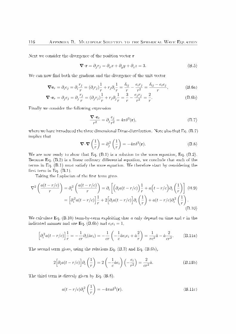
116 Appendix B. Multipole Solution to the Spherical Wave Equation
Next we consider the divergence of the position vector r
∇·r = ∂jrj = ∂xx+ ∂yy + ∂zz = 3. (B.5)
We can now find both the gradient and the divergence of the unit vector
∇er = ∂iej = ∂irjr
= (∂irj)1r
+ rj∂i1r
=δijr− eirj
r2=δij − eiej
r, (B.6a)
∇·er = ∂jej = ∂jrjr
= (∂jrj)1r
+ rj∂j1r
=3r− ejrj
r2=
2r. (B.6b)
Finally we consider the following expression
∇·err2
= ∂jejr2
= 4πδ3(r), (B.7)
where we have introduced the three dimensional Dirac-distribution. Note also that Eq. (B.7)implies that
∇·∇(
1r
)= ∂ 2
j
(1r
)= −4πδ3(r). (B.8)
We are now ready to show that Eq. (B.1) is a solution to the wave equation, Eq. (B.2).Because Eq. (B.2) is a linear ordinary differential equation, we conclude that each of theterms in Eq. (B.1) must satisfy the wave equation. We therefore start by considering thefirst term in Eq. (B.1).
Taking the Laplacian of the first term gives
∇2
(a(t− r/c)
r
)= ∂ 2
i
(a(t− r/c)
r
)= ∂i
[(∂ia(t− r/c)
)1r
+ a(t− r/c
)∂i
(1r
)](B.9)
=[∂ 2i a(t− r/c)
]1r
+ 2[∂ia(t− r/c)
]∂i
(1r
)+ a(t− r/c)∂ 2
i
(1r
).
(B.10)
We calculate Eq. (B.10) term-by-term exploiting that a only depend on time and r in theindicated manner and use Eq. (B.6b) and eiei = 1,[
∂ 2i a(t− r/c)
]1r
= − 1cr∂i(aei) = − 1
cr
(−1caeiei + a
2r
)=
1rc2
a− a 2cr2
. (B.11a)
The second term gives, using the relations Eq. (B.3) and Eq. (B.6b),
2[∂ia(t− r/c)
]∂i
(1r
)= 2
(−1caei
)(− eir2
)=
2cr2
a. (B.11b)
The third term is directly given by Eq. (B.8),
a(t− r/c)∂ 2i
(1r
)= −4πaδ3(r). (B.11c)

Appendix B. Multipole Solution to the Spherical Wave Equation 117
From Eq. (B.10) and Eq. (B.11) we can now calculate the left-hand side of the waveequation Eq. (B.2) for the first term of the considered solution Eq. (B.1)[
∇2 − 1c2∂ 2t
](a(t− r/c)
r
)=[
1rc2
a− a 2cr2
+ a2cr2− 4πaδ3(r)
]− 1rc2
a (B.12)
= −4πaδ3(r). (B.13)
We conclude that the first term of Eq. (B.1) is in fact a solution to the wave equation, exceptfor the expected divergence in polar coordinates when we let r go to zero — representedwith the Dirac-distribution.
Next we consider whether the second term of Eq. (B.1) is a solution to the scalar waveequation. Taking the Laplacian of this term yields
∇2
[∇·(
A(t− r/c)r
)]= ∂ 2
i
[(∂jAj)
1r
+Aj∂j
(1r
)](B.14a)
= ∂i
[(∂i∂jAj)
1r
+ (∂jAj)∂i
(1r
)+ (∂iAj)∂j
(1r
)+Aj∂i∂j
(1r
)](B.14b)
= (∂i∂i∂jAj)1r
+ (∂i∂jAj)∂i
(1r
)+ (∂i∂jAj)∂i
(1r
)+ (∂jAj)∂i∂i
(1r
)+ (∂i∂iAj)∂j
(1r
)+ (∂iAj)∂i∂j
(1r
)+ (∂iAj)∂i∂j
(1r
)+Aj∂i∂i∂j
(1r
) (B.14c)
= (∂i∂i∂jAj)1r
+ 2(∂i∂jAj)∂i
(1r
)+ (∂jAj)∂i∂i
(1r
)+ (∂i∂iAj)∂j
(1r
)+ 2(∂iAj)∂i∂j
(1r
)+Aj∂i∂i∂j
(1r
).
(B.14d)
For simplicity we have omitted the arguments of the vector A.To keep track of the following calculations we calculate each term in Eq. (B.14d) seper-
ately using the relations Eq. (B.3) to Eq. (B.8). The first term gives(∂i∂i∂jAj
)1r
= − 1rc∂i∂i
(Ajej
)=
1rc∂i
(1cAjeiej − Aj
δij − eiejr
)(B.15a)
=1c2r
(∂iAj)eiej +1c2r
Aj(∂iei)ej +1c2r
Ajei(∂iej)
− (∂iAj)δij − eiej
cr2− Aj
∂iδij − (∂iei)ej − ei(∂iej)cr2
(B.15b)
= − 1c3r
...Ajeieiej +
1c2r
Aj2rej +
1c2r
Ajeiδij − eiej
r
+...Aei
δij − eiejc2r2
− Aj−2rej − ei
δij−eiej
r
cr2.
(B.15c)
We notice that eiδij = ej and eiei = 1 which reduces Eq. (B.15c) to
− 1c3r
...Ajej +
2c2r2
Ajej +2cr3
Ajej . (B.16)

118 Appendix B. Multipole Solution to the Spherical Wave Equation
Continuing with the calculation of the second term in Eq. (B.14d) exploiting that we havecalculated ∂i∂jAj in Eq. (B.15a) gives
2(∂i∂jAj
)∂i
(1r
)= 2
(1c2Ajeiej − Aj
δij − eiejcr
)(− eir2
)= − 2
c2r2Ajej . (B.17)
Considering the third and sixth term together using Eq. (B.8) we write(∂jAj
)∂i∂i
(1r
)+Aj∂i∂i∂j
(1r
)= −4π(∂jAj)δ
3(r)− 4πAj[∂jδ
3(r)](B.18a)
= −4π∂j[Ajδ
3(r)]. (B.18b)
Next we consider the fourth term
(∂i∂iAj)∂j
(1r
)= ∂i
(−1cAjei
)(−ejr2
)(B.19a)(
1c2Ajeiei −
1cAj
2r
)(−ejr2
)= − 1
c2r2Ajej +
2cr3
Ajej , (B.19b)
and the fifth term gives
2(∂iAj
)∂i∂j
(1r
)= 2
(−1cAjej
)∂i
[−ejr2
](B.20a)
= 2(
1cAjej
)[(∂iej)
1r2
+ ej∂i
(1r2
)](B.20b)
= 2(
1cAjej
)[(δij − eiej
r
)1r2
+ ej
(−2
1r3
)](B.20c)
= − 4cr3
Ajej . (B.20d)
Inserting the obtained results into the original expression for the Laplacian of
∇·(A(t− r/c)/r), (B.21)
we get
∇2
[∇·(
A(t− r/c)r
)]= − 1
c3r
...Ajej +
2c2r2
Ajej +2cr3
Ajej −2c2r2
Ajej
− 4π∂j[Ajδ
3(r)]− 1c2r2
Ajej +2cr3
Ajej −4cr3
Ajej
(B.22a)
= − 1c3r
...Ajej −
1c2r2
Ajej − 4π∂j[Ajδ
3(r)]. (B.22b)
Next step in confirming that the term ∇·(A(t − r/c)/r) is indeed a solution to the waveequation is calculating the double time-derivative,
∂ 2t
[∇·(A(t− r/c)
r)
]= ∂ 2
t
[(∂jAj)
1r
+Aj∂j
(1r
)](B.23a)
= ∂ 2t
[− 1rcAjej −
1r2Ajej
]= − 1
rc
...Ajej −
1r2Ajej . (B.23b)

Appendix B. Multipole Solution to the Spherical Wave Equation 119
Inserting the calculated terms Eq. (B.22b) and Eq. (B.23b) into the wave equation, Eq. (B.2),we get
− 1c3r
...Ajej −
1c2r2
Ajej − 4π∂j[Ajδ
3(r)]− 1c2
(− 1rc
...Ajej −
1r2Ajej
)= −4π∂j
[Ajδ
3(r)]
= −4π∇·[Aδ3(r)
].
(B.24)
Thus we have shown that the second term of Eq. (B.1) also fulfills the wave equation exceptat the origin, where we have the expected divergence due to the choice of polar coordinates.
Because the wave equation is linear, we can now from Eq. (B.13) and Eq. (B.24)conclude that Eq. (B.1) is a solution to the wave equation everywhere except at the originwhere the divergence is taken care of by the delta-functions.

120 Appendix B. Multipole Solution to the Spherical Wave Equation

Appendix C. Scattered Wave From Incoming Traveling Plane Wave 121
Appendix C
Scattered Wave From Incoming
Traveling Plane Wave
In this appendix we find and expression for the scattered wave from an incoming plane wave,as we describe in Section 5.3. We consider the incoming traveling plane wave described bythe velocity potential
φin(x, t) = −u0
kcos(kx− ωt). (C.1)
This gives the incoming velocity field as the gradient of Eq. (C.1)
vin = (∂xφin)ex = u0 sin(kx− ωt)ex = vin,0ex, (C.2)
where we have defined vin,0 as the amplitude of the incoming field in the x-direction.Importantly we notice that the time derivative of the velocity potential can be written interms of this component in the following way:
∂tφin = −u0ω
ksin(kx− ωt) = −cavin,0. (C.3)
We can from the incoming velocity potential determine the scattered potential of Eq. (5.36)using that from Eq. (C.3) we have
ρin = −ρ0
c2a∂tφin =
ρ0
cavin,0. (C.4)
This gives us
φsc(t− r/ca) = − R3
3carf1vin,0(t− r/ca)−
R3
2f2∇·
(vin(t− r/ca)
r
). (C.5)
We neglect terms of higher orders in r, because we are not considering r values close tothe origin (inside the sphere). Noting that the dot notation implies differentiation withrespect to the argument, we get
φsc(t− r/ca) = − R3
3carf1vin,0(t− r/ca) +
R3
2carf2vin(t− r/ca)·er +O(r−2). (C.6)

122 Appendix C. Scattered Wave From Incoming Traveling Plane Wave
The velocity is then given as the gradient of Eq. (C.6)
vsc(t− r/ca) = ∇φsc(t− r/ca) (C.7)
=(R3
3c2arf1vin,0(t− r/ca)−
R3
2c2arf2vin(t− r/ca)·er
)er +O(r−2) (C.8)
= vsc,0er +O(r−2), (C.9)
where we have defined vsc,0 as the radial component of the scattered velocity.Using the incoming velocity
vin(t− r/ca) = −u0 sin[ω(t− r/ca)
]ex, (C.10)
and taking the double-derivative we get
vin(t− r/ca) = u0ω2 sin
[ω(t− r/ca)
]ex = vin,0ex, (C.11)
the scattered velocity field is found by inserting into Eq. (C.8),
vsc(t− r/ca) =(R3
3c2arf1u0ω
2 sin[ω(t− r/ca)
]− R3
2c2arf2u0ω
2 sin[ω(t− r/ca)
]ex ·er
)er
=R3u0ω
2
c2arsin[ω(t− r/ca)
](13f1 −
12f2 cos θ
)er. (C.12)
As was the case for the time derivative of the incoming velocity potential, the scatteredvelocity potential can be expressed by the component of the scattered velocity field
∂tφsc
(t− r/ca
)= − R3
3carf1vin,0
(t− r/ca
)+
R3
2carf2vin,0
(t− r/ca
)er = −cavsc,0 (C.13)
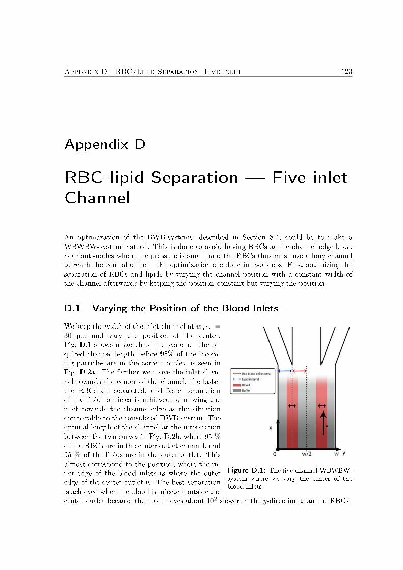
Appendix D. RBC/Lipid Separation, Five-inlet 123
Appendix D
RBC-lipid Separation — Five-inlet
Channel
An optimazation of the BWB-systems, described in Section 8.4, could be to make aWBWBW-system instead. This is done to avoid having RBCs at the channel edged, i.e.near anti-nodes where the pressure is small, and the RBCs thus must use a long channelto reach the central outlet. The optimization are done in two steps: First optimizing theseparation of RBCs and lipids by varying the channel position with a constant width ofthe channel afterwards by keeping the position constant but varying the position.
D.1 Varying the Position of the Blood Inlets
Figure D.1: The five-channel WBWBW-system where we vary the center of theblood inlets.
We keep the width of the inlet channel at winlet =30 µm and vary the position of the center.Fig. D.1 shows a sketch of the system. The re-quired channel length before 95% of the incom-ing particles are in the correct outlet, is seen inFig. D.2a. The farther we move the inlet chan-nel towards the center of the channel, the fasterthe RBCs are separated, and faster separationof the lipid particles is achieved by moving theinlet towards the channel edge as the situationcomparable to the considered BWB-system. Theoptimal length of the channel at the intersectionbetween the two curves in Fig. D.2b, where 95 %of the RBCs are in the center outlet channel, and95 % of the lipids are in the outer outlet. Thisalmost correspond to the position, where the in-ner edge of the blood inlets is where the outeredge of the center outlet is. The best separationis achieved when the blood is injected outside thecenter outlet because the lipid moves about 102 slower in the y-direction than the RBCs.

124 Appendix D. RBC/Lipid Separation, Five-inlet
(a) (b)
Figure D.2: (a) A five-inlet system with winlet = 30 µm where we vary the center of the bloodinlet. The dashed line indicates the split between the inner and outer outlet channel. (b) Zoomof (a) to see the intersection between the two curves and thus the optimal separation length.
D.2 Varying the Width of the Blood Inlets
To see if we can optimize the separation by using smaller blood inlet channel, we considera fixed center of the blood inlet at ycenter = 87.5 µm (corresponding to the maximum ofthe pressure force) and vary the width of the blood inlet channel; a sketch of the systemis shown in Fig. D.3a, and the results can be seen in Fig. D.3b. We see that the requiredlength of the channel grows as we make the inlets larger. This is due to the fact thatwe inject particles farther and farther away from the outlet splitting point and where thepressure force is smaller the wider we make the inlet. If we again compare with the BWB-system, we conclude that the required length of the channel is not noticeably shorter. Ifwe for instance picked a design with an inlet 60 µm wide, i.e. yinlet ∈ [57.5 µm; 117.5 µm],we would get approximately the same channel length as for the BWB-system. Howeverthis would lead to a flow rate, Qblood = 1.91 × 10⁻⁹ m3/s = 0.12 mL/min, or only 60 %of the BWB-design or approximately 40 % of the one-inlet design. Thus we conclude thatthis five-inlet system is not the optimal choice if we want a high throughput since a bigpart of the inlets are filled with buffer.
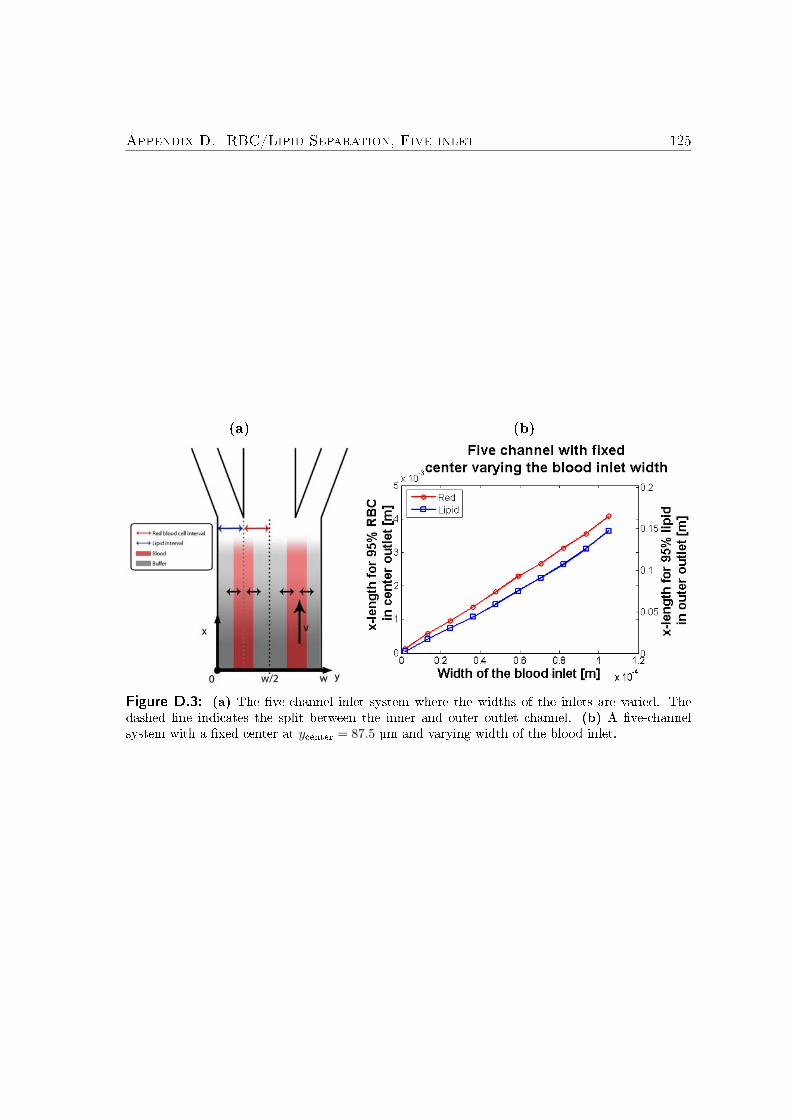
Appendix D. RBC/Lipid Separation, Five-inlet 125
(a) (b)
Figure D.3: (a) The five-channel inlet system where the widths of the inlets are varied. Thedashed line indicates the split between the inner and outer outlet channel. (b) A five-channelsystem with a fixed center at ycenter = 87.5 µm and varying width of the blood inlet.

126 Appendix D. RBC/Lipid Separation, Five-inlet

Appendix E. Derivation of the Acoustic Streaming Term 127
Appendix E
Derivation of the Acoustic
Streaming Term
In Section 12.8 we found that the governing equations of the boundary layer problemoutline in the section was given as
∂tv1,x − ν∂2yv1,x = ∂tU1(x), (E.1a)
ν∂2y〈v2,x〉 =
⟨v1,x∂xv1,x
⟩+⟨v1,y∂yv1,x
⟩−⟨U1(x)∂xU1(x)
⟩. (E.1b)
To solve those for the single solid-boundary problem considered in Section 12.8 we start bysolving the first-order problem, as this enters into the second-order equation Eq. (E.1b).
We assume a first-order stationary standing wave in the region outside the boundaryregion,
U1(x) = U0 cos(kx) e−iωt, (E.2)
where we have used complex notation for convenience, remembering to take the real partat the end.
This implies that the first-order equation for the velocity Eq. (E.1a) becomes a second-order inhomogeneous partial differential equation in time and y,
∂tv1,x − ν∂2yv1,x = −iωU0 cos(kx) e−iωt. (E.3)
The boundary condition for this partial differential equation is that the velocity mustremain finite as y approach infinity i.e. |v1,x| < ∞ for y → ∞. At the other boundaryy = 0 we employ the usual no-slip condition at the solid wall (which we for conveniencehave placed at y = 0), such that v1,x = 0 for y = 0.
We assume for the time dependence that the first-order perturbation in velocity os-cillates in phase with the oscillations in the main stream, i.e. that the first-order velocityperturbation has a harmonic time dependence. Given this condition we search for a solutionto Eq. (E.3) of the form,
v1,x = F (y)U0 cos(kx) e−iωt, (E.4)
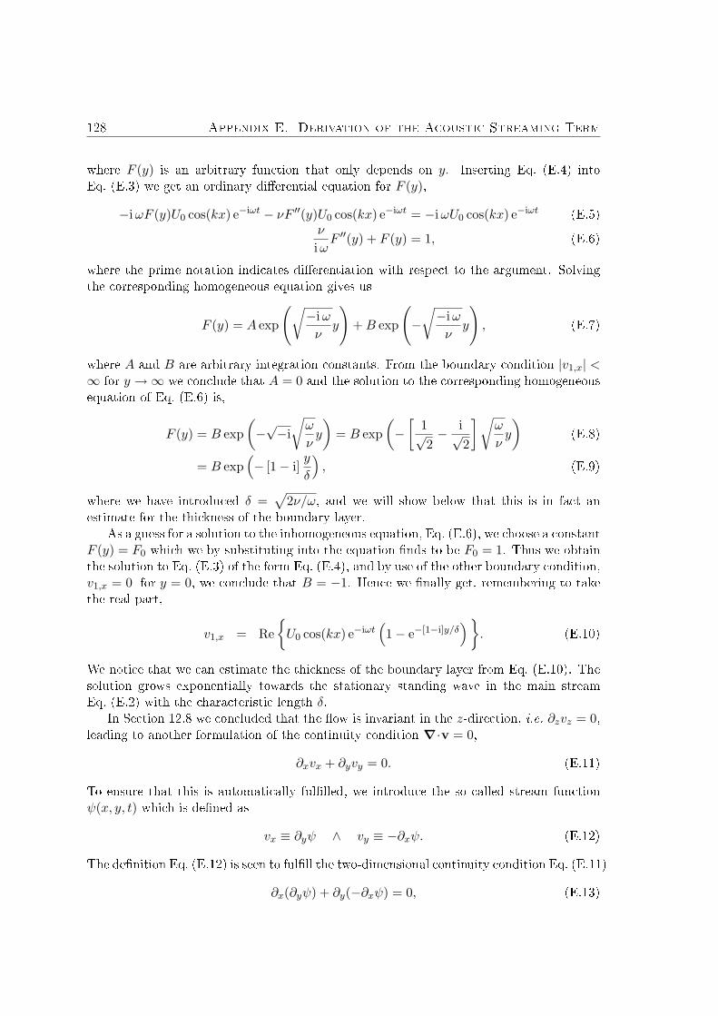
128 Appendix E. Derivation of the Acoustic Streaming Term
where F (y) is an arbitrary function that only depends on y. Inserting Eq. (E.4) intoEq. (E.3) we get an ordinary differential equation for F (y),
−iωF (y)U0 cos(kx) e−iωt − νF ′′(y)U0 cos(kx) e−iωt = −iωU0 cos(kx) e−iωt (E.5)ν
iωF ′′(y) + F (y) = 1, (E.6)
where the prime notation indicates differentiation with respect to the argument. Solvingthe corresponding homogeneous equation gives us
F (y) = A exp
(√−iων
y
)+B exp
(−√−iων
y
), (E.7)
where A and B are arbitrary integration constants. From the boundary condition |v1,x| <∞ for y →∞ we conclude that A = 0 and the solution to the corresponding homogeneousequation of Eq. (E.6) is,
F (y) = B exp(−√−i√ω
νy
)= B exp
(−[
1√2− i√
2
]√ω
νy
)(E.8)
= B exp(− [1− i]
y
δ
), (E.9)
where we have introduced δ =√
2ν/ω, and we will show below that this is in fact anestimate for the thickness of the boundary layer.
As a guess for a solution to the inhomogeneous equation, Eq. (E.6), we choose a constantF (y) = F0 which we by substituting into the equation finds to be F0 = 1. Thus we obtainthe solution to Eq. (E.3) of the form Eq. (E.4), and by use of the other boundary condition,v1,x = 0 for y = 0, we conclude that B = −1. Hence we finally get, remembering to takethe real part,
v1,x = Re{U0 cos(kx) e−iωt
(1− e−[1−i]y/δ
)}. (E.10)
We notice that we can estimate the thickness of the boundary layer from Eq. (E.10). Thesolution grows exponentially towards the stationary standing wave in the main streamEq. (E.2) with the characteristic length δ.
In Section 12.8 we concluded that the flow is invariant in the z-direction, i.e. ∂zvz = 0,leading to another formulation of the continuity condition ∇·v = 0,
∂xvx + ∂yvy = 0. (E.11)
To ensure that this is automatically fulfilled, we introduce the so called stream functionψ(x, y, t) which is defined as
vx ≡ ∂yψ ∧ vy ≡ −∂xψ. (E.12)
The definition Eq. (E.12) is seen to fulfill the two-dimensional continuity condition Eq. (E.11)
∂x(∂yψ) + ∂y(−∂xψ) = 0, (E.13)

Appendix E. Derivation of the Acoustic Streaming Term 129
as long as the velocity and stream function are connected via Eq. (E.12). The first-orderstream function ψ1 corresponding to Eq. (E.10) is given from Eq. (E.12) via integration,where we take ψ1 = 0 for y = 0 equivalent to the earlier mentioned condition v1,x =0 for y = 0,
ψ1(x, y, t) = Re
{U0 cos(kx) e−iωt
(y +
e−κy
κ
)}= Re
{U0 cos(kx) e−iωtC1(y)
}, (E.14)
where we for notation simplicity have introduced κ = [1− i] /δ and C1(y) = (y + e−κy/κ).From this stream function the first-order velocity component in the y-direction can bederived from Eq. (E.12),
v1,y = Re{U0k sin(kx) e−iωtC1(y)
}. (E.15)
We have now derived the first-order perturbations to the velocity, and from Eq. (E.1b) wecan now find the second-order perturbation. We turn our attention to the right-hand side ofEq. (E.1b) and first focus on the time-dependence. We notice that the terms have the formconsidered in Section 3.5, such that the time average of the product of A(t) = Re
{A0e
iωt}
and B(t) = Re{B0e
iωt}is given as, Eq. (3.55),⟨
A(t)B(t)⟩
=12Re [A0B
∗0 ] , (E.16)
where the prime denotes complex conjugation.Carrying out the spatial differentiation of the expressions given in Eqs. (E.2), (E.10),
and (E.15) respectively, we get
ν∂2y〈v2,x〉 = −1
2U2
0k cos(kx) sin(kx) Re{C ′1(y)C
′∗1 (y)
}+
12U2
0k cos(kx) sin(kx) Re{C1(y)C ′′∗1 (y)
}+
12U2
0k cos(kx) sin(kx).
(E.17)
Using that cos(α) sin(α) = 1/2 sin(2α) we reduce Eq. (E.17) to,
ν∂2y〈v2,x〉 =
14U2
0k sin(2kx)[1 + Re
{C1(y)C ′′∗1 (y)
}− |C ′∗1 |2
]. (E.18)
We notice from earlier that C1(y) = (y + e−κy/κ) and κ = [1− i] /δ so that the right-handside of Eq. (E.18) is known, and we by two-fold integration in y get
ν〈v2,x〉 =14U2
0k sin(2kx)[12δye−y/δ cos(y/δ)− 2δ2e−y/δ sin(y/δ)
− 12δye−y/δ sin(y/δ)− 1
4e−2y/δδ2 +Ay +B
],
(E.19)
where A and B are arbitrary integration constants with respect to y.

130 Appendix E. Derivation of the Acoustic Streaming Term
It is clear that the second-order time-averaged velocity must stay finite at all timesindicating the boundary condition |v2,x| < ∞ for y → ∞. Exploiting this boundarycondition, we get A = 0 in Eq. (E.19). Furthermore we still apply the no-slip conditionat the boundary of the solid wall, implying that also v2,x = 0 for y = 0. Using this inEq. (E.19) we conclude that B = δ2/4.
Far from the boundary layer we therefore have the velocity field due to the viscid effectsat the boundary,
ν〈v2,x〉∣∣∣∞
=116U2
0k sin(2kx)δ2 ⇔ 〈v2,x〉∣∣∣∞
=18U2
0
casin(2kx), (E.20)
where we in the last equality have used that the wavenumber in the acoustic wave outsidethe boundary layer is k = ω/ca, and that we have already concluded that the characteristiclength of the boundary layer could be expressed as δ =
√2ν/ω.

Appendix F. Temperature Dependence 131
Appendix F
Temperature Dependence of
Viscosity and Speed of Sound
In Section 12.4 we determine the temperature dependence of η and of the Φ-factor. Thevalue of η for different temperatures is found in [8] and given in Table F.1. The temperaturedependence is taken from [17] and is also shown in Table F.1.
Table F.1: Viscosity of blood and speed of sound in water as a function of temperature.
τ [◦C] η [mPa s] ca [ m s−1]
0 - 1401.010 - 1447.820 - 1483.222 3.4 -25 - 1497.430 - 1509.537 2.7 -40 2.4 1528.450 - 1541.460 - 1549.570 - 1553.280 - 1552.8

132 Appendix F. Temperature Dependence

Appendix G. Gor’kov’s Article 133
Appendix G
Gor’kov’s Article
Here follows the original Gor’kov article from 1962, [14]. It should be noted that this is ascanned document, since we have not been able to find it electronically.


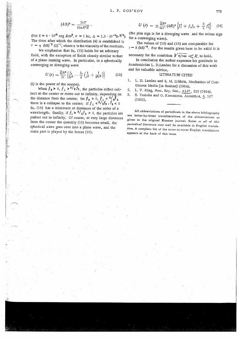
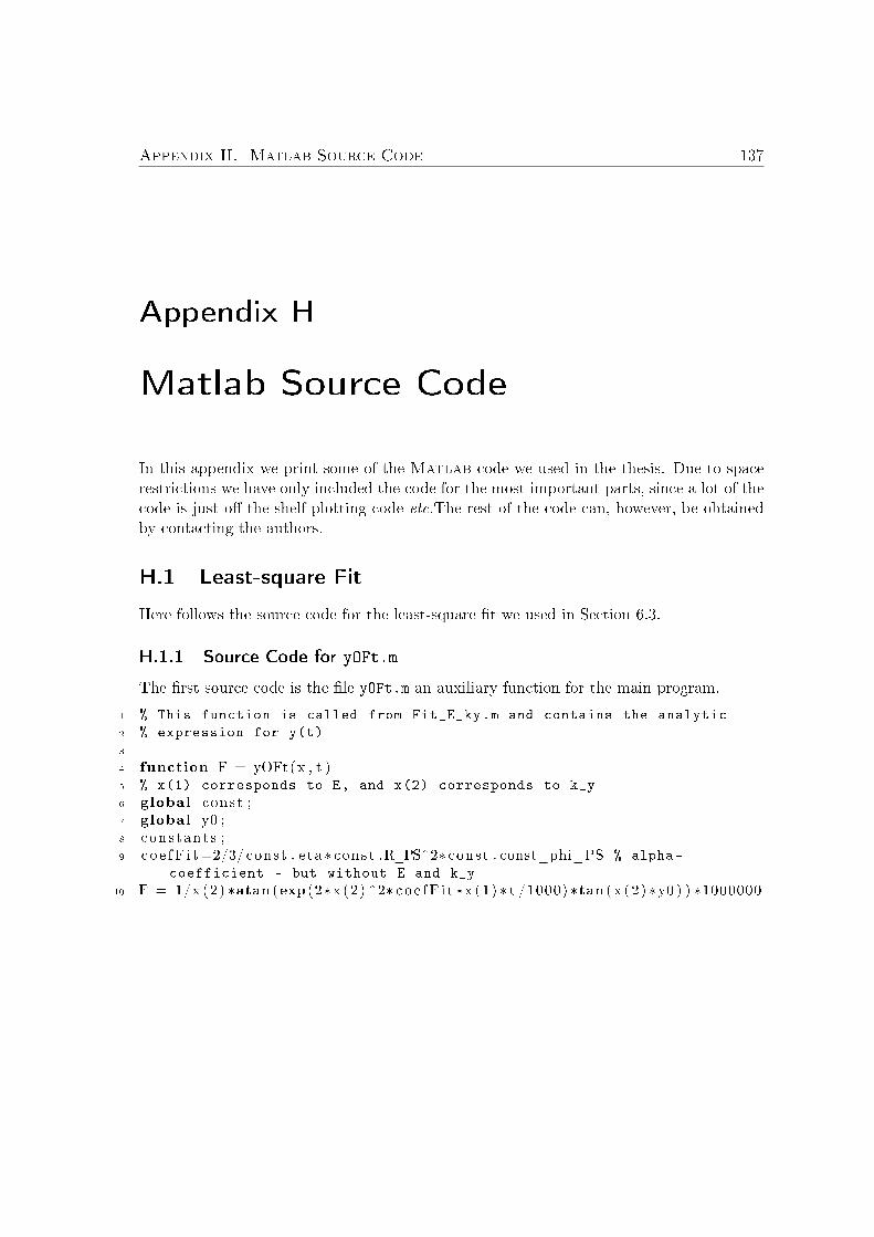
Appendix H. Matlab Source Code 137
Appendix H
Matlab Source Code
In this appendix we print some of the Matlab code we used in the thesis. Due to spacerestrictions we have only included the code for the most important parts, since a lot of thecode is just off-the-shelf plotting code etc.The rest of the code can, however, be obtainedby contacting the authors.
H.1 Least-square Fit
Here follows the source code for the least-square fit we used in Section 6.3.
H.1.1 Source Code for yOFt.m
The first source code is the file yOFt.m an auxiliary function for the main program.
1 % This function is called from Fit_E_ky.m and contains the analytic
2 % expression for y(t)
3
4 function F = yOFt(x , t )5 % x(1) corresponds to E, and x(2) corresponds to k_y
6 global const ;7 global y0 ;8 cons tant s ;9 c o e fF i t =2/3/ const . eta * const .R_PS^2* const . const_phi_PS % alpha-
coefficient - but without E and k_y
10 F = 1/x (2 ) *atan (exp(2*x (2 ) ^2* c o e fF i t *x (1 ) * t /1000) *tan ( x (2 ) *y0 ) ) *1000000

138 Appendix H. Matlab Source Code
H.1.2 Source Code for Fit_E_ky.m
This is the source code for the main function in our least-square fit analysis.
1 %%%% Script Fit_E_ky.m %%%%
2 % Makes a two-parameter fit of E and k_y from particle trajectory y(t)
from
3 % a particle affected by pressure force
4
5 clear a l l ;6 close a l l ;7 % All lengths are in um and times in ms
8 global const9 global y0
10
11 % Loading of the data
12 cons tant s ;13 load PartA_1V_bred % Data must be from left side of channel, otherwise
uncomment the following line
14 %part(:,2)=377-part(:,2);
15 y0=part (1 , 2 ) *1e−6;16
17 % Sets the options for the curve fit
18 opt ions = opt imset ( ’ t o l x ’ ,1 e−18, ’ t o l f un ’ ,1 e−18) ;19 lb = [ 0 0 ] ;20 ub = [1000 200000 ] ;21 [ x , resnorm ] = l s q c u r v e f i t ( ’ yOft ’ , [ 2 0 8000 ] , part ( : , 1 ) , part ( : , 2 ) , lb , ub ,
opt ions ) ;22
23 % Fit of the data
24 t t f i t=linspace ( part (1 ) , part ( length ( part ( : , 1 ) ) ) ,1000) ;25 y y f i t =1./x (2 ) *atan (exp(2*x (2 ) * const . coef_PS .* x (1 ) .* t t f i t /1000) .* tan ( x
(2 ) *y0 ) ) *1000000;26
27 % Plot of the data
28 f igure (1 ) ;29 plot ( part ( : , 1 ) , part ( : , 2 ) , ’ ok ’ , t t f i t , yy f i t , ’−b ’ ) ;30 legend ( ’Exp . r e s u l t ’ , ’MATLAB f i t ’ , 4 ) ;31 xlabel ( ’ t [ms ] ’ ) ;32 ylabel ( ’ y [ \mu{m} ] ’ ) ;33
34 E=x (1)35 ky=x (2)36 lambda=2*pi/x (2 )37
38 t i t l e ( [ ’ F i t o f t r a j e c t o r y in channel with width w=’ num2str( const .w*1 e6) ’ \mu{m} where E=’ num2str(E) ’ J/m^3 and \lambda/2= ’ num2str(lambda*1 e6 /2) ’ \mu{m} ’ ] )

Appendix H. Matlab Source Code 139
H.2 Simulation of Single-particle in Rectangular Channel
This is the basic code for the simulations of the single-particles in our rectangular channelincluding the source file we used for all the constants.
H.2.1 Source Code for constants.m
This is the source code for all the constants we used in our simulation
1 %%%% constants.m %%%%
2 % A common file containing the constants we use in the simulations
3
4 global const5
6 % Diameter of RBC is 6-8 um, thickness is 2 um, so volumes are
7 % approximately 50 - 100 um^3
8 V_red=75e−18; % m
9 % Converting to a radius when assuming spherical RBCs
10 const . R_red=(V_red*3/4/pi ) ^(1/3) ; % m
11 const . R_lipid=1.5e−6; % m
12 % WBCs are approximately spherical in shape, range from about 5 to 20
um in
13 % diameter. 10 um is a good average diameter
14 const .R_whi=5e−6; % m
15 % Radius of polystyrene
16 const .R_PS=2.58e−6; % m
17
18 % Here we use the viscosity of blood
19 const . eta =0.0027; % Pa s
20 % Density of blood
21 const . rho_0=1052.2; % kg m^(-3)
22 % Speed of sound in water
23 const . c=1483; % m s^(-1)
24 % Densities of the particles
25 const . rho_s_red=1096; %kg m^(-3);
26 const . rho_s_lipid=920; %kg m^(-3);
27 const . rho_s_whi=1060; %kg m^(-3);
28
29 % Compressibilities
30 const . beta_0=5.88e−10 % Pa^(-1)
31 const . beta_red=3.48e−10; % Pa^(-1)
32 const . be ta_l ip id =5.34e−10; % % Pa^(-1)
33 % We assume that beta_whi=beta_red
34 const . beta_whi=const . beta_red ; % % Pa^(-1)
35
36 % Calculating the Phi-factors
37 const . const_phi_red=(( const . rho_s_red+2/3*( const . rho_s_red−const . rho_0 )) /(2* const . rho_s_red+const . rho_0 )−1/3* const . beta_red/ const . beta_0 ) ;
38 const . const_phi_l ip id=(( const . rho_s_lipid+2/3*( const . rho_s_lipid−const .rho_0 ) ) /(2* const . rho_s_lipid+const . rho_0 )−1/3* const . be ta_l ip id /const . beta_0 ) ;

140 Appendix H. Matlab Source Code
39 const . const_phi_whi=(( const . rho_s_whi+2/3*( const . rho_s_whi−const . rho_0 )) /(2* const . rho_s_whi+const . rho_0 )−1/3* const . beta_whi/ const . beta_0 ) ;
40 const . const_phi_PS=0.226;41
42 % Channel parameters
43 % Height
44 const . h=125e−6; % m
45 % Width
46 const .w=350e−6; % m
47 % The wavenumber , assuming that we have half a wavelength
48 const . k=pi/ const .w; % m^(-1)
49
50 % We assume that the incoming wave is given as
51 % phi=-u_0/k*cos(omega*t)*cos(k*x)
52 % Amplitude of the potential
53 const . u_0=100; % m s^(-1)
54 const .E=1000; % J m^(-3)
55
56 % The change in pressure per unit length
57 const . del_p_L=3e5 ; % Pa m^(-1)
58
59 % The flow-rate using the first term
60 Q=const . h^3* const .w* const . deltaP_flow_over_L/12/ const . eta *(1−192/pi^5*const . h/ const .w*tanh (pi* const .w/(2* const . h ) ) ) % m^3/s
61 mLprMin=Q*60*1 e6 % mL min^(-1)
62 % The average velocity in the x-direction
63 v_x=Q/ const . h/ const .w % m s^(-1)
64
65 % How many terms to include in the pousielle flow
66 const . o r d e rPou s e i l l e =4;
H.2.2 Source Code for Pos_Equation.m
This file calculates the derivatives we use in our ode45-function. It is an auxiallry functionfor CalcPosition.m.
1 %%%% Script Pos_Equation.m %%%%
2 % Set-up of the differential -equations in our problem
3 % They will later be used in the ode45 method
4
5 function dpos=Pos_Equation ( t , pos )6
7 %Loads constants
8 global const9 global part_nr
10
11 %Define the velocity-vector, dpos(2) is the y-component and dpos(1) the
12 %x-component
13 dpos=zeros ( 2 , 1 ) ;14

Appendix H. Matlab Source Code 141
15 % Get the right differential -equations in the y-direction from the
particle
16 % number
17 i f part_nr==1 %RBC
18 const . coef_red=2/3/ const . eta * const .E* const . k* const . R_red^2* const .const_phi_red ;
19 dpos (2 )=const . coef_red * sin (2* const . k*pos (2 ) ) ;20 e l s e i f part_nr==2 %Lipid
21 const . c o e f_ l i p i d=2/3/ const . eta * const .E* const . k* const . R_lipid^2*const . const_phi_l ip id ;
22 dpos (2 )=const . c o e f_ l i p i d * sin (2* const . k*pos (2 ) ) ;23 e l s e i f part_nr ==3 %WBC
24 const . coef_whi=2/3/ const . eta * const .E* const . k* const .R_whi^2* const .const_phi_whi ;
25 dpos (2 )=const . coef_whi* sin (2* const . k*pos (2 ) ) ;26 else27 disp ( [ ’ Choose a va l i d p a r t i c l e ! ’ ] )28 end29
30 %Pouseille flow at z=h/2
31 for i i =1: const . o r d e rPou s e i l l e32 nn=i i *2−1;33 dpos (1 )=dpos (1 )+1/(nn)^3*(1−cosh (nn*(pi *( pos (2 )−const .w/2) ) / const . h
) /cosh (nn*pi* const .w/(2* const . h ) ) ) *(−1) ^((nn−1)/2) ;34 end35 dpos (1 )=dpos (1 ) *4* const . h^2* const . del_p_L/(pi^3* const . eta ) ;

142 Appendix H. Matlab Source Code
H.2.3 Source Code for CalcPosition.m
In this file we find the required x-length and time for a particle to go from ystart to yend.It requires the scripts Pos_Equation.m and constants.m.
1 %%%% Script CalcPosition.m %%%%
2 % Calculates the particle trajectories using the ode45 function and our
3 % function Pos_Equation.m
4
5 % Returns the positions and times given a y_start, y_end, and a
particle
6 % number
7 function [ Tslut , Xslut ] = Ca lcPos i t i on ( y_start , y_end , p a r t i c l e )8
9 % Loads our constants file
10 global const11 global part_nr12
13 % 1 is RBC, 2 is Lipid, and 3 is WBC
14 part_nr=p a r t i c l e ;15
16 % Options for the ode45 function including tolerances
17 opt ions = odeset ( ’ RelTol ’ ,1 e−12, ’ AbsTol ’ , [ 1 e−12 1e−12]) ;18 % The time-interval we are looking at
19 TimeLength=100;20
21 % Solving the differtial equations using our Pos_Equation.m
22 [T, y]=ode45 (@Pos_Equation , [ 0 TimeLength ] , [ 0 y_start ] , opt ions ) ;23
24 Tslut=0;25 Xslut=0;26
27 % Finding the required lengths before particles are at y_end
28 i f p a r t i c l e==1 | p a r t i c l e ==3 % For RBC and WBC
29 i nd ex s l u t=min( find ( y ( : , 2 )>y_end) ) ;30 ttemp=T( index s l u t ) ;31 xtemp=y( indexs lu t , 1 ) ;32
33 % If the particles reaches y_end return time and x-position
34 i f isnan ( ttemp ) == 035 Tslut=ttemp ;36 end37
38 i f isnan ( xtemp) == 039 Xslut=xtemp ;40 end41 e l s e i f p a r t i c l e==2 % For lipids
42 i nd ex s l u t=min( find ( y ( : , 2 )<y_end) ) ;43 ttemp=T( index s l u t ) ;44 xtemp=y( indexs lu t , 1 ) ;45

Appendix H. Matlab Source Code 143
46 % If the particles reaches y_end return time and x-position
47 i f isnan ( ttemp ) == 048 Tslut=ttemp ;49 end50
51 i f isnan ( xtemp) == 052 Xslut=xtemp ;53 end54 end
144 Appendix H. Matlab Source Code

Bibliography 145
Bibliography
[1] Private conversation with Jacob Riis Folkenberg at the company FOSS.
[2] Private communication with the Thomas Laurell group at Lund University, Sweden.
[3] Private conversation with the group of H. T. Soh at University Center Santa Barbara.
[4] Rune Barnkob. Acoustofluidics in Microsystems. Master’s thesis, DTU (TechnicalUniversity of Denmark), 2009.
[5] Henrik Bruus. Theoretical Microfluidics. Oxford University Press, Oxford, 2008.
[6] Henrik Bruus, Jonathan Adams, and H. T. Soh. Continuous separation of red andwhite blood cells by acoustic radiation forces from transverse, standing ultrasoundwaves in a microfluidic channel. Unpublished note., 2008.
[7] C. G. Caro, T. J. Pedley, R. C. Schroter, and W. A. Seed. The Mechanics of theCirculation. Oxford University Press, 1978.
[8] Yildirim Çinar et al. Blood viscosity and blood pressure: Role of temperature andhyperglycemia. American Journal of Hypertension, 14(5):433–438, 2001.
[9] Lawrence A. Crum. Bjerkness forces on bubbles in a stationary sound field. TheAcoustical Society of America, 57(6):Part 1, 1975.
[10] Leopold Dintenfass. Blood viscosity, hyperviscosity, and hyperviscosaemia. Springer,1985.
[11] R. L. Earle. Unit operations in food processing. http://www.nzifst.org.nz/
unitoperations/flfltheory4.htm, visited 2nd of June. Main page: www.nzifst.
org.nz.
[12] Glenn Elert. Density of blood. http://hypertextbook.com/facts/2004/
MichaelShmukler.shtml, visited 1st of June. Main page: http://www.
hypertextbook.com.
[13] Martin A. M. Gijs. Magnetic bead handling on-chip: new opportunities for analyticalapplications. Microfluidics and Nanofluidics, 1:22–40, 2004.
[14] L.P. Gor’kov. On the forces acting on a small particle in an acoustic field in an idealfluid. Doklady Akedemii Nauk SSSR, 140(1):88–91, 1961.

146 Bibliography
[15] Louis V. King. On the acoustic radiation pressure on spheres. Mathematical andPhysical Sciences, 147(861):212–240, 1934.
[16] L.D. Landau and E.M. Lifshitz. Fluid mechanics, Volume 6 of Course of TheoreticalPhysics. Pergamon Press, New York, 1987.
[17] David Lide. CRC Handbook of Chemistry and Physics, 89th edition. Taylor andFrancis Group, 2009.
[18] Miguel Moyers-Gonzales, Robert G. Owens, and Jiannong Fang. A non-homogeneousconstitutive model for human blood. part 1. model derivation and steady flow. J.Fluid Mech., 617:327–354, 2008.
[19] Nicole Pamme. Magnetism and microfluidics. Lab on a Chip, 6:24–38, 2005.
[20] William K. Purves, David Sadava, Gordon H. Orians, and H. Craig Heller. Life: TheScience of Biology. Sinauer Associates, Sunderland, 2004.
[21] H. Roginski, J. W. Fuquay, and P. F. Fox. Encyclopedia of Dairy Sciences. AcademicPress, 2003.
[22] Peder Skafte-Pedersen. Acoustic forces on particles and liquids in microfluidic systems.Master’s thesis, DTU (Technical University of Denmark), 2008.
[23] A. R. Pries et al. Blood flow in microvascular networks. Experiments and simulation.Circ. Res., 67:826–834, 1990.
[24] Andreas Nilsson et al. Acoustic control of suspended particles in micro fluidic chips.Lab Chip, 4:131–135, 2004.
[25] A.R. Pries et al. Blood viscosity in tube flow: dependence on diameter and haemat-ocrit. Am. J. Physiol, 263:H1770–H1778, 1992.
[26] C. Grenvall et al. Harmonic microchip acoustophoresis - a route to on line raw milksample precondition in protein and lipid content quality control. Submitted for Ana-lytical Chemistry.
[27] Dwayne A. Johnson et al. Methodology for fractionating suspended particles usingultrasonic standing wave and divided flow fields. Separations Technology, 5:251–258,1995.
[28] Filip Petersson et al. Separation of lipids from blood utilizing ultrasonic standingwaves in microfluidic channels. The Analyst, 129(1):938–943, 2004.
[29] Filip Petersson et al. Continuous separation of lipid particles from erythrocytes bymeans of laminar flow and acoustic standing wave forces. Lab on a Chip, 5:20–22,2005.
[30] Filip Petersson et al. Free flow acoustophoresis: Microfluidic-based mode of particleand cell separation. Analytical Chemistry, 79(14):5117–5123, 2007.
Bibliography 147
[31] J. Hultström et al. Proliferation and viability of adherent cells manipulated bystanding-wave ultrasound in a microfluidic chip. Ultrasound in Medicine and Biology,33(1):145–151, 2007.
[32] Jeremy J. Hawkes et al. Force field particle filter, combining ultrasound standing waveand laminar flow. Sensors and Actuators B, 75:213–222, 2001.
[33] J.F. Spengler et al. Observation of yeast cell movement and aggregation in a small-scale mhz ultrasonic standing wave field. Bioseparation, 9(6):329–341, 2001.
[34] Kyuichi Yasui et al. Strongly interacting bubbles under an ultrasonic horn. PhysicalReview, E 77:016609, 2008.
[35] M.Z. Bazant et al. Diffuse-charge dynamics in electrochemical systems. PhysicalReview, E 70(021506):1–24, 2004.
[36] M.Z. Bazant et al. Induced-charge electrokinetic phenomena: Theory and microfluidicapplications. Physical Review, 92(066101):1–4, 2004.
[37] N.R. Harris et al. A silicon ultrasonic microfluidic separator. Sensors and Actuators,B 95:425–434, 2003.
[38] Per Augustsson et al. Buffer medium exchange in continuous cell and particle streamsusing ultrasonic standing wave focusing. Springer-Verlag, pages 269–277, 2008.
[39] R. Mettin et al. Bjerkness forces between small cavitation bubbles in a strong acousticfield. Physical Review, 56(3):2924–2931, 1997.
[40] T. S. Simonova et al. Low-frequency dielectrophoresis and the polarization interac-tion of uncharged spherical particles with an induced debye atmosphere of arbitrarythickness. Colloid Journal, 63(1):108–115, 2001.
[41] Thomas L. Tolt et al. Separation of dispersed phases from liquids in acousticallydriven chambers. Chemical Engineering Science,, 48(3):521–540, 1993.
[42] Thomas Laurell et al. Chip integrated strategies for acoustic separation and manipu-lation of cells and particles. Chemical Society Reviews, 36:492–506, 2007.
[43] K. Yosioka and Y. Kawasima. Acoustic radiation pressure on a compressible sphere.Acustica, 5(3):167–173, 1955.