Master Thesis, s072160

Theory and Simulation ofElectrokinetics in Micro- and

Nanochannels

Christoffer P. Nielsen

Supervisor: Professor Henrik BruusCo-supervisor: Mathias Bækbo Andersen

Department of Micro- and NanotechnologyTechnical University of Denmark

June 29, 2012

Abstract

In this thesis we present results from a numerical study of the effects of surface reactionsand bulk reactions on the ion transport across nanoporous ion-selective membranes inmicrochannels. Transport across such membranes plays an important role for dialysisdevices, fuel cells, lab-on-a-chip devices and a number of industrial chemical processes[1, 2, 3, 4].

Although ion-selective membranes have been studied for almost a century proper mod-elling of their transport properties remains a challenging task. This is both due to thenonlinearity of the governing equations and to the host of mechanisms, which affect thetransport. One such mechanism, which has not yet been investigated, is the effect ofsurface reactions in the microchannels connecting to the membrane.

In the course of the investigations we find that the surface reactions give rise to a vary-ing differential conductance in the so-called overlimiting regime of ion transport througha membrane. We rationalise this and other findings using a combination of analyticalresults and physical understanding.

Using the developed electrokinetic models we also attempt to simulate the operation ofa desalination device with a novel design. No conclusion as to the viability of the design ishowever arrived at, as the desalination device is found to rely critically on a complicatedasymmetric geometry, which cannot be modelled using the employed axisymmetric 3Dmodel.

III

Dansk resume

I denne afhandling præsenterer vi resultater fra et numerisk studie af effekterne af kemiskereaktioner pa ion-transport igennem nanoporøse ion-selektive membraner i mikrokanaler.Ion-transport pa tværs af sadanne membraner spiller en vigtig rolle for dialyse apparater,brændselsceller, lab-on-a-chip systemer og adskillige industrielle kemiske processer [1, 2,3, 4].

Selvom ion-selektive membraner er blevet studeret i næsten hundrede ar er det stadigvanskeligt at modellere deres transportegenskaber ordentligt. Dette skyldes bade at destyrende ligninger er stærkt ikke-lineære og at der er en lang række mekanismer sompavirker transporten. En sadan mekanisme, som endnu ikke er blevet undersøgt, er effek-ten af overfladereaktioner i de mikrokanaler der leder op til membranen.

Vores undersøgelser viser at overfladereaktionerne giver anledning til en varierendedifferentiel ledningsevne i det sakaldte ’overbegrænsede’ regime for ion-transport igennemen ion-selektiv membran. Vi forklarer mekanismerne bag denne og andre effekter vha.analytiske resultater og simple fysiske argumenter.

Vi forsøger endvidere at anvende de udviklede elektrokinetiske modeller til at simulereet afsaltningsapparat med et nyskabende design. Vi nar dog ikke frem til nogen konklu-sion angaende designets egnethed, da det bliver klart at afsaltningsapparatet er kritiskafhængigt af en kompliceret asymmetrisk geometri, som ikke kan modelleres vha. denanvendte aksesymmetriske 3D model.

V

Preface

The present thesis is submitted as fulfilment of the prerequisites for obtaining the Master ofScience and Engineering degree at the Technical University of Denmark (DTU). The workhas been carried out at the Department of Micro- and Nanotechnology (DTU Nanotech)in the Theoretical Microfluidics Group (TMF) headed by professor Henrik Bruus. Thework on this 50 ECTS credits project was carried out from September 2011 to June 2012.

I have several people to thank for help and support during this project. First andforemost, I would like to thank my supervisor Professor Henrik Bruus and my co-supervisorMathias Bækbo Andersen. The experience and general physical insight of Henrik Bruus aswell as Mathias’s in-depth understanding of electrokinetic phenomena have been invaluableto the completion of this project.

I am grateful to the entire TMF group for making a great working environment, whichallows for both serious study and for cutting loose in a bar or a paintball arena. Also, thewealth of LATEX and Matlab knowledge accumulated in the group has been a great help.

Finally, I would like to thank my four roommates Dea, Nils, Niels Ole and Birgitte forlots of support, hot meals and a healthy amount of distraction from the thesis writing.

Christoffer P. NielsenDepartment of Micro- and Nanotechnology

Technical University of Denmark29 June 2012

VII

Contents

Abstract . . . . . . . . . . . . . . . . . . . . . . . . . . . . . . . . . . . . . . . . IIIDansk resume . . . . . . . . . . . . . . . . . . . . . . . . . . . . . . . . . . . . . VPreface . . . . . . . . . . . . . . . . . . . . . . . . . . . . . . . . . . . . . . . . . VIIList of Figures . . . . . . . . . . . . . . . . . . . . . . . . . . . . . . . . . . . . . XList of Tables . . . . . . . . . . . . . . . . . . . . . . . . . . . . . . . . . . . . . XIIList of Symbols . . . . . . . . . . . . . . . . . . . . . . . . . . . . . . . . . . . . XV

1 Introduction 11.1 Electrokinetics . . . . . . . . . . . . . . . . . . . . . . . . . . . . . . . . . . 11.2 Ion-selective membranes . . . . . . . . . . . . . . . . . . . . . . . . . . . . 2

2 Theory 42.1 Governing equations . . . . . . . . . . . . . . . . . . . . . . . . . . . . . . 4

2.1.1 The continuum hypothesis . . . . . . . . . . . . . . . . . . . . . . . 42.1.2 Fluid dynamical equations . . . . . . . . . . . . . . . . . . . . . . . 52.1.3 Electrostatic equations . . . . . . . . . . . . . . . . . . . . . . . . . 62.1.4 Transport equations . . . . . . . . . . . . . . . . . . . . . . . . . . 72.1.5 Current density revisited . . . . . . . . . . . . . . . . . . . . . . . . 7

2.2 Chemical reactions . . . . . . . . . . . . . . . . . . . . . . . . . . . . . . . 112.2.1 Bulk reactions . . . . . . . . . . . . . . . . . . . . . . . . . . . . . . 112.2.2 Surface reactions . . . . . . . . . . . . . . . . . . . . . . . . . . . . 13

3 Physical Modelling 17

4 Analytical Modelling 204.1 The diffuse part of the screening layer . . . . . . . . . . . . . . . . . . . . . 204.2 Overlimiting current in a microchannel . . . . . . . . . . . . . . . . . . . . 214.3 Dynamic surface charge density . . . . . . . . . . . . . . . . . . . . . . . . 244.4 Hydronium distribution . . . . . . . . . . . . . . . . . . . . . . . . . . . . 25

5 Numerical Modelling 295.1 The finite element method . . . . . . . . . . . . . . . . . . . . . . . . . . . 295.2 Comsol . . . . . . . . . . . . . . . . . . . . . . . . . . . . . . . . . . . . . 335.3 Mesh Convergence . . . . . . . . . . . . . . . . . . . . . . . . . . . . . . . 33

IX

CONTENTS

6 An effective 1D model for ion transport 356.1 Modelling of the effective 1D problem . . . . . . . . . . . . . . . . . . . . . 35

6.1.1 1D model of the membrane . . . . . . . . . . . . . . . . . . . . . . 386.2 Implementation of the 1D model . . . . . . . . . . . . . . . . . . . . . . . . 396.3 Results . . . . . . . . . . . . . . . . . . . . . . . . . . . . . . . . . . . . . . 41

6.3.1 Zero surface charge density . . . . . . . . . . . . . . . . . . . . . . . 416.3.2 Constant surface charge density . . . . . . . . . . . . . . . . . . . . 416.3.3 Dynamic surface charge density . . . . . . . . . . . . . . . . . . . . 45

7 Axisymmetric 3D model 507.1 Implementation of the 2D model . . . . . . . . . . . . . . . . . . . . . . . . 507.2 Results . . . . . . . . . . . . . . . . . . . . . . . . . . . . . . . . . . . . . . 51

8 A coupled 1D-2D model for the ion transport 548.1 Coupling of 1D and 2D model . . . . . . . . . . . . . . . . . . . . . . . . . 548.2 Implementation of the coupled 1D-2D model . . . . . . . . . . . . . . . . . 568.3 Results . . . . . . . . . . . . . . . . . . . . . . . . . . . . . . . . . . . . . . 57

9 Desalination device 609.1 Implementation . . . . . . . . . . . . . . . . . . . . . . . . . . . . . . . . . 619.2 Results . . . . . . . . . . . . . . . . . . . . . . . . . . . . . . . . . . . . . . 62

10 Conclusion and Outlook 66

X

List of Figures

1.1 Sketch of dialysis device . . . . . . . . . . . . . . . . . . . . . . . . . . . . 2

1.2 Sketch of simple system containing an ion-selective membrane . . . . . . . 3

2.1 Hydration of an ionic compound . . . . . . . . . . . . . . . . . . . . . . . . 12

2.2 Sketch of the electric screening layer . . . . . . . . . . . . . . . . . . . . . 15

2.3 Sketch of the potential in the screening layer . . . . . . . . . . . . . . . . . 15

3.1 Sketch of a system including michrochannels and an ion-selective membrane 18

3.2 Sketch of the model system used in the thesis . . . . . . . . . . . . . . . . 19

4.1 Gouy-Chapman solution for the potential in the diffuse layer. . . . . . . . . 21

4.2 Sketch of auto-dissociation of water close to an ion-selective membrane . . 26

4.3 Influence of the salt ions on the water ions. . . . . . . . . . . . . . . . . . . 27

4.4 Depletion of hydronium in the bulk microchannel. . . . . . . . . . . . . . . 27

5.1 Sketch of a linearly varying basis function. . . . . . . . . . . . . . . . . . . 30

5.2 Basis function representations of a sine function. . . . . . . . . . . . . . . . 30

5.3 Mesh convergence plot. . . . . . . . . . . . . . . . . . . . . . . . . . . . . . 34

6.1 Build up of a numerical instability. . . . . . . . . . . . . . . . . . . . . . . 40

6.2 I-V curves for model with no surface charge. . . . . . . . . . . . . . . . . . 42

6.3 Cation concentration and space charge density in a model with no surfacecharge and no water ions. . . . . . . . . . . . . . . . . . . . . . . . . . . . 42

6.4 Cation concentration and space charge density in a model with no surfacecharge. . . . . . . . . . . . . . . . . . . . . . . . . . . . . . . . . . . . . . . 43

6.5 Hydronium concentration and water ion space charge density in a modelwith no surface charge. . . . . . . . . . . . . . . . . . . . . . . . . . . . . . 43

6.6 I-V curves for a model with constant surface charge density. . . . . . . . . 43

6.7 Cation and hydronium concentration profiles for a model with constantsurface charge density. . . . . . . . . . . . . . . . . . . . . . . . . . . . . . 44

6.8 Current plotted versus the surface charge density. . . . . . . . . . . . . . . 45

6.9 Surface charge density in a microchannel as a function of ionic strength andpH. . . . . . . . . . . . . . . . . . . . . . . . . . . . . . . . . . . . . . . . . 46

XI

LIST OF FIGURES

6.10 I-V characteristics for a model with dynamic surface charge density andR = 1µm. . . . . . . . . . . . . . . . . . . . . . . . . . . . . . . . . . . . . 47

6.11 I-V characteristics for a model with dynamic surface charge density andR = 5µm. . . . . . . . . . . . . . . . . . . . . . . . . . . . . . . . . . . . . 47

6.12 Axial cation concentration in a model with dynamic surface charge andR = 5µm. . . . . . . . . . . . . . . . . . . . . . . . . . . . . . . . . . . . . 48

6.13 Dynamic surface charge density in a model with R = 5µm. . . . . . . . . . 486.14 Axial cation concentration for varying inlet concentrations. . . . . . . . . . 49

7.1 Meshing of the 2D domain . . . . . . . . . . . . . . . . . . . . . . . . . . . 517.2 I-V curve for 2D model with and without advection. . . . . . . . . . . . . . 527.3 Cation concentration and velocity field in a 2D model. . . . . . . . . . . . 53

8.1 Sketch of the model system illustrating which regions are being modelled using a 2D

model and which regions are modelled using a 1D model. . . . . . . . . . . . . . . 568.2 I-V curves for a 2D model and a 1D-2D model. . . . . . . . . . . . . . . . 588.3 Cation concentration for a 2D model and a 1D-2D model. . . . . . . . . . . 588.4 Velocity fields for a 2D model and a 1D-2D model. . . . . . . . . . . . . . 598.5 I-V curve for a 1D-2D model of a channel with dynamic surface charge and

R = 0.6µm. . . . . . . . . . . . . . . . . . . . . . . . . . . . . . . . . . . . 598.6 Axial cation concentration for a 1D-2D model of a channel with dynamic

surface charge and R = 0.6µm. . . . . . . . . . . . . . . . . . . . . . . . . 59

9.1 Model of a desalination device. . . . . . . . . . . . . . . . . . . . . . . . . 619.2 Salt concentration at the side channel outlet for c0 = 1 mM. . . . . . . . . 639.3 Axial cation concentration in a desalination device for c0 = 1 mM. . . . . . 639.4 Cation concentration in a desalination device for c0 = 1 mM. . . . . . . . 649.5 Magnitude of the current density in a desalination device for c0 = 1 mM. . 649.6 Salt concentration at the side channel outlet for c0 = 600 mM. . . . . . . . 65

XII

List of Tables

2.1 Bare and hydrated radii of some common ions. . . . . . . . . . . . . . . . . 12

XIII

XIV

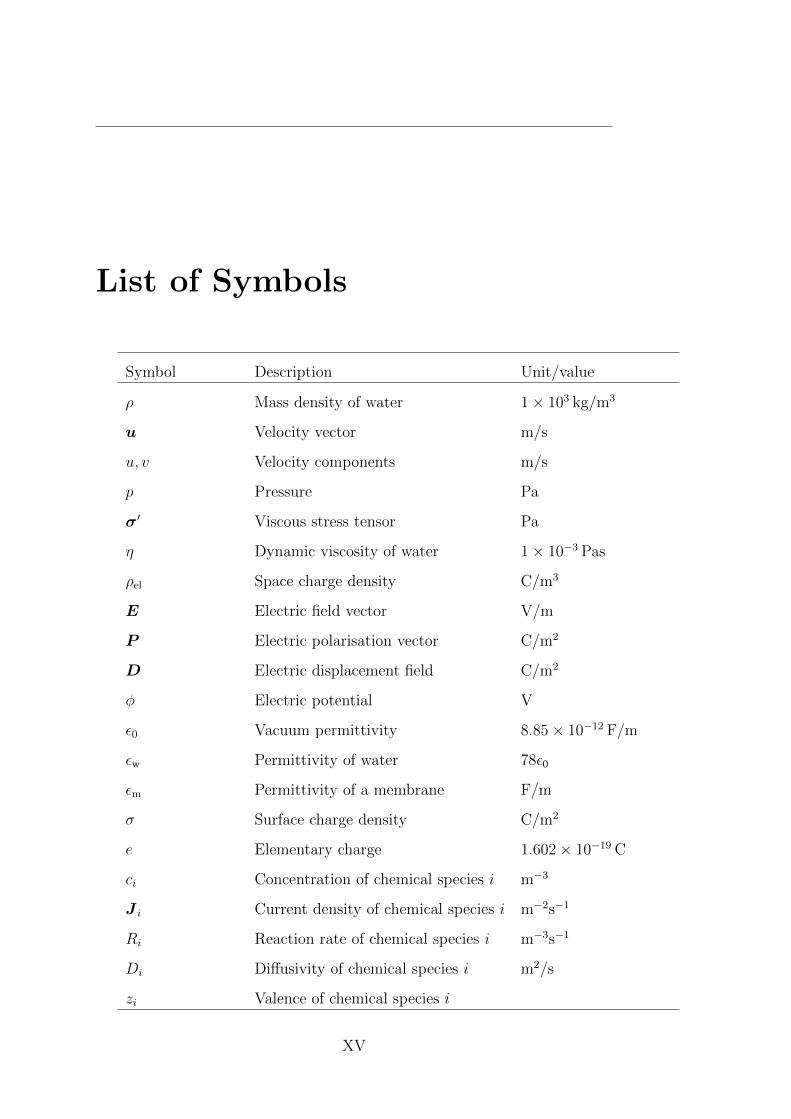
List of Symbols

Symbol Description Unit/value

ρ Mass density of water 1× 103 kg/m3

u Velocity vector m/s

u, v Velocity components m/s

p Pressure Pa

σ′ Viscous stress tensor Pa

η Dynamic viscosity of water 1× 10−3 Pas

ρel Space charge density C/m3

E Electric field vector V/m

P Electric polarisation vector C/m2

D Electric displacement field C/m2

φ Electric potential V

ε0 Vacuum permittivity 8.85× 10−12 F/m

εw Permittivity of water 78ε0

εm Permittivity of a membrane F/m

σ Surface charge density C/m2

e Elementary charge 1.602× 10−19 C

ci Concentration of chemical species i m−3

J i Current density of chemical species i m−2s−1

Ri Reaction rate of chemical species i m−3s−1

Di Diffusivity of chemical species i m2/s

zi Valence of chemical species i

XV

LIST OF SYMBOLS

Symbol Description Unit/value

kB Boltzmann constant 1.38× 10−23 J/K

T Temperature 300 K

VT = kBTze

Thermal voltage 25.7 mV (for z = 1)

µi Electrochemical potential of chemical species i V

Li Generalised mobility of chemical species i m2/Vs

F Helmholtz Free energy J

U Internal energy J

S Entropy J/K

ai Ionic radius of chemical species i m

p0 Water dipole moment 4.79 D

cH, [H3O+] , [H+] Hydronium concentration m−3

cOH,[OH−

]Hydroxide concentration m−3

Kw Self-ionization constant of water 1× 10−14 M2

Γi Surface density of chemical species i m−2

Cs Stern capacitance 2.9 F/m2

εP Porosity of membrane

τ Tortuosity of membrane

Nm Density of unit charges in membrane m−3

ρm Space charge density of membrane C/m3

ζ, φd Potential at the compact layers outer edge V

λD Debye length m

Lic Length of inlet channel m

Lm Length of membrane m

Loc Length of outlet channel m

R Radius of microchannel m

c0 Salt concentration at reservoir m−3

XVI

Chapter 1

Introduction

The topic of the present thesis Theory and Simulation of Electrokinetics in Micro- andNanochannels is the study of electrokinetic phenomena and in particular the study ofmicrosystems containing nanoporous ion-selective membranes. Below a short introductionto the field of electrokinetics will be given, followed by an introduction to ion-selectivemembranes.

1.1 Electrokinetics

Consider a particle of positive charge suspended in a liquid. Such a particle may besubjected to a number of different forces. If the particle is small enough Brownian motionwill induce it to move randomly about. If the liquid starts to move the particle willbe dragged along with the liquid. If an electric field is applied the particle will moveunder the influence of the Lorentz force, and if there is a nearby wall of negative charge,the particle will move towards the wall. The study of how these forces affect systemscontaining electrolytes or charged particles is called electrokinetics.

Phenomena relying on electrokinetics are ubiquitous in nature since all living organismscontain large amounts of ionic liquid, and for instance the nervous system is criticallydependent on electrokinetics for its function [1]. Electrokinetic phenomena also have awide array of industrial and technological applications, e.g. in battery technology, lab-on-a-chip devices, chemical sensing, bioanalytics and dialysis [1, 2, 3, 4].

A prominent feature of electrokinetic systems are the so-called screening layers whichdevelop next to surfaces. The screening layers are a response to the surface charge den-sity, which many materials acquire through chemical reactions when submerged in anelectrolyte. To screen this surface charge, ions of opposite charge move towards the in-terface and ions of like charge move away from the interface. Thermal motion of the ionsprevent most of them from adsorbing on the surface, and as a result a diffuse screeninglayer forms next to the surface. These screening layers are important for the ion transportin a system because they, in contrast with the largely charge neutral bulk liquid, can havea quite high space charge density.

1

1. Introduction

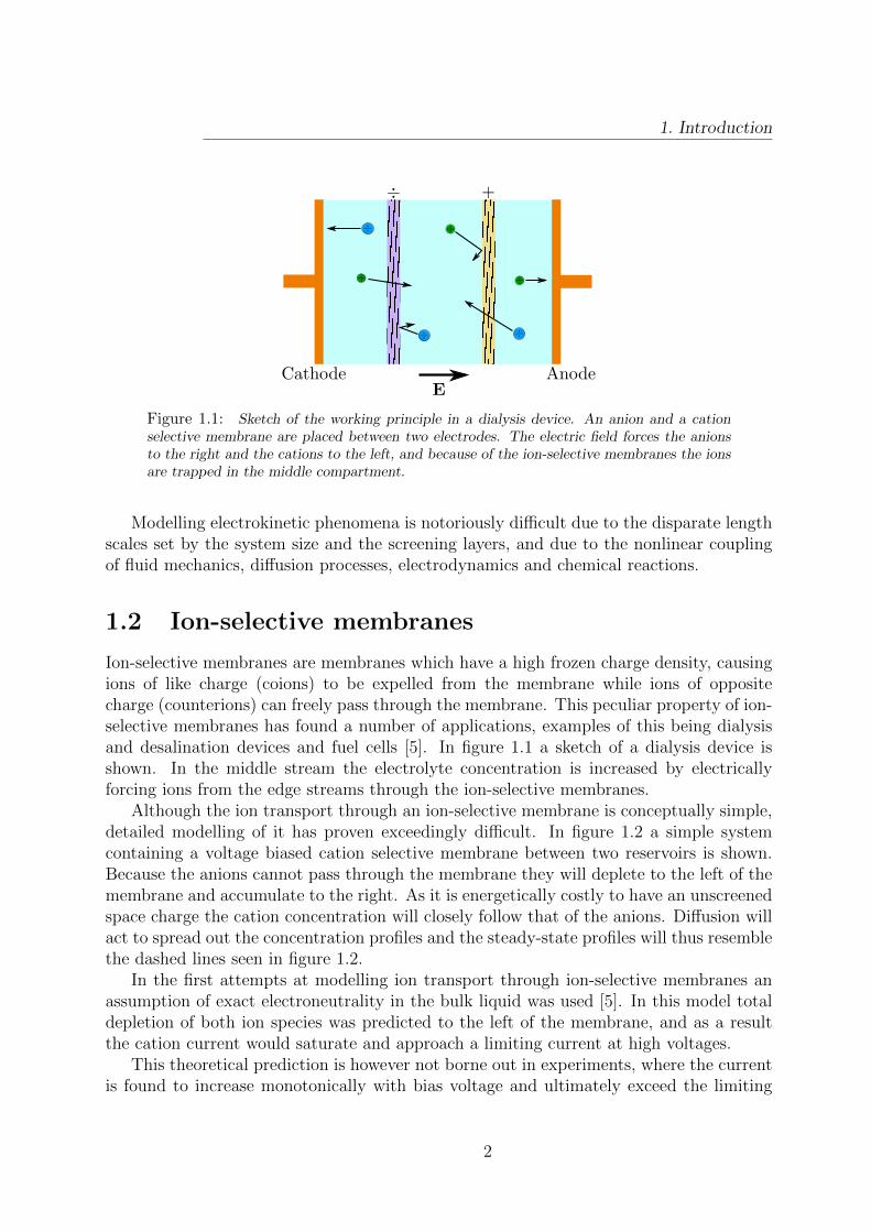
Figure 1.1: Sketch of the working principle in a dialysis device. An anion and a cationselective membrane are placed between two electrodes. The electric field forces the anionsto the right and the cations to the left, and because of the ion-selective membranes the ionsare trapped in the middle compartment.

Modelling electrokinetic phenomena is notoriously difficult due to the disparate lengthscales set by the system size and the screening layers, and due to the nonlinear couplingof fluid mechanics, diffusion processes, electrodynamics and chemical reactions.

1.2 Ion-selective membranes

Ion-selective membranes are membranes which have a high frozen charge density, causingions of like charge (coions) to be expelled from the membrane while ions of oppositecharge (counterions) can freely pass through the membrane. This peculiar property of ion-selective membranes has found a number of applications, examples of this being dialysisand desalination devices and fuel cells [5]. In figure 1.1 a sketch of a dialysis device isshown. In the middle stream the electrolyte concentration is increased by electricallyforcing ions from the edge streams through the ion-selective membranes.

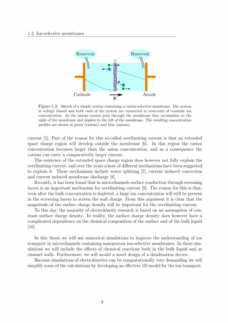
Although the ion transport through an ion-selective membrane is conceptually simple,detailed modelling of it has proven exceedingly difficult. In figure 1.2 a simple systemcontaining a voltage biased cation selective membrane between two reservoirs is shown.Because the anions cannot pass through the membrane they will deplete to the left of themembrane and accumulate to the right. As it is energetically costly to have an unscreenedspace charge the cation concentration will closely follow that of the anions. Diffusion willact to spread out the concentration profiles and the steady-state profiles will thus resemblethe dashed lines seen in figure 1.2.

In the first attempts at modelling ion transport through ion-selective membranes anassumption of exact electroneutrality in the bulk liquid was used [5]. In this model totaldepletion of both ion species was predicted to the left of the membrane, and as a resultthe cation current would saturate and approach a limiting current at high voltages.

This theoretical prediction is however not borne out in experiments, where the currentis found to increase monotonically with bias voltage and ultimately exceed the limiting

2

1.2. Ion-selective membranes

Figure 1.2: Sketch of a simple system containing a cation-selective membrane. The systemis voltage biased and both ends of the system are connected to reservoirs of constant ionconcentration. As the anions cannot pass through the membrane they accumulate to theright of the membrane and deplete to the left of the membrane. The resulting concentrationprofiles are shown in green (cations) and blue (anions).

current [5]. Part of the reason for this so-called overlimiting current is that an extendedspace charge region will develop outside the membrane [6]. In this region the cationconcentration becomes larger than the anion concentration, and as a consequence thecations can carry a comparatively larger current.

The existence of the extended space charge region does however not fully explain theoverlimiting current, and over the years a host of different mechanisms have been suggestedto explain it. These mechanisms include water splitting [7], current induced convectionand current induced membrane discharge [8].

Recently, it has been found that in microchannels surface conduction through screeninglayers is an important mechanism for overlimiting current [9]. The reason for this is that,even after the bulk concentration is depleted, a large ion concentration will still be presentin the screening layers to screen the wall charge. From this argument it is clear that themagnitude of the surface charge density will be important for the overlimiting current.

To this day, the majority of electrokinetic research is based on an assumption of con-stant surface charge density. In reality, the surface charge density does however have acomplicated dependence on the chemical composition of the surface and of the bulk liquid[10].

In this thesis we will use numerical simulations to improve the understanding of iontransport in microchannels containing nanoporous ion-selective membranes. In these sim-ulations we will include the effects of chemical reactions both in the bulk liquid and atchannel walls. Furthermore, we will model a novel design of a desalination device.

Because simulations of electrokinetics can be computationally very demanding we willsimplify some of the calculations by developing an effective 1D model for the ion transport.

3

Chapter 2

Theory

In this chapter the theory applied in the remainder of the report is introduced, andimportant concepts and their significance are presented.

The chapter starts with a discussion of the continuum hypothesis in which the appro-priateness of employing continuum models is considered. The basic continuum equationsdescribing the motion of the liquid, the distribution of the electrical potential and thetransport of solvents are then presented. Finally, the modelling of chemical reactions inbulk and at surfaces is treated. This part includes a discussion of the screening layers andintroduces the standard model used to describe these.

2.1 Governing equations

2.1.1 The continuum hypothesis

The systems we want to study are mixtures of ions and water which may be subject toexternal electrical fields. A full description of such systems requires individual modellingof all molecules and their mutual forces, which for typical microscopic system volumesbetween 10 fL and 1 nL means carrying out simulations involving up toN ∼ 1016 molecules.Although the computation time of the most efficient molecular dynamics algorithms onlyscale as O(N), it is not feasible to perform molecular dynamics simulations of systemswith this many particles.

For most applications, knowledge of the detailed behaviour of the constituent moleculesmay however not be important, because the outcome of any measurement on the systemwill be an average over a large number of molecules. A theory which only describes themolecular properties on average will thus be sufficient for many purposes. In such a theorythe behaviour of the system is described via continuous fields, and the assumption thatthis gives an adequate description is called ’the continuum hypothesis’.

The justification of the continuum hypothesis can be assessed by considering a so-calledfluid particle, which is the domain over which molecules are sampled to give the field valueat a given point. To minimise fluctuations in the physical fields such a fluid particle must

4

2.1. Governing equations

be large enough to sample many molecules. On the other hand the fluid particle mustbe much smaller than the representative physical length scales, so that external forces donot cause the physical properties to vary within the fluid particle. The size of the fluidparticle is thus constrained from above and from below. Demanding that the relativedeviations due to statistical fluctuations are less than 1 percent, the minimum size of thefluid particle is given as [2]

λ∗ ∼ (0.01)−2/3n−1/3, (2.1)

where n is the molecular concentration. For water this characteristic length is around6.7 nm.

The continuum hypothesis starts to break down, when the physically relevant lengthscales approach this lower bound on the fluid particle size. This may very well be an issuewhen studying electrokinetic systems, as the characteristic size of the screening layers canbe in the sub-nanometer range. In lack of efficient alternatives we will not let that deterus from employing continuum models in the study of elektrokinetic systems, as physicallysound albeit inaccurate conclusions may still be extracted from such models. We will thusproceed with developing the continuum theory of electrokinetics, while keeping in mindthat caution has to be taken when interpreting results in regions where the continuumhypothesis is invalid.

2.1.2 Fluid dynamical equations

The equations governing the motion of a fluid are continuity equations, expressing theconservation of mass and momentum. The first of these is simply called the continuityequation and reads

∂tρ = −∇ · (ρu), (2.2)

where ρ and u are the density and velocity of the fluid. Liquids are only weakly compress-ible and for the velocity fields typically encountered in microfluidics they can to a verygood approximation be treated as incompressible. The continuity equation thus reducesto

∇ · u = 0. (2.3)

The momentum density at a given point in a fluid can change by advection of momentumor by the application of external forces. The momentum conservation equation thereforehas the form

∂t(ρu) = ∇ · [−ρuu− pI + σ′] + fbody, (2.4)

where ρuu is the advection term, p is the pressure in the fluid, σ′ is the viscous stresstensor and fbody is a sum of any other body forces which might be present. The viscousstress tensor is given as

σ′ = η[∇u+ (∇u)T

]+ (β − 1)η(∇ · u)I, (2.5)

5

2. Theory

where η is the dynamic viscosity and β is a dimensionless viscosity ratio. Since we aredealing with incompressible fluids the last term in the viscous stress tensor can be ne-glected.

We will be studying systems with small length scales and low velocities, meaning thatthe Reynolds number, Re = ρV0L0

η, is much smaller than unity. Also, we will only be

considering systems in steady-state, so the momentum conservation equation reduces tothe steady Stokes equation

∇ · [−pI + σ′] + fbody = 0. (2.6)

In the systems we will be studying the relevant body forces are gravitational forces andelectrostatic forces. The first of these is cancelled by the hydrostatic pressure, leaving onlythe electrostatic force given as

f el = ρelE. (2.7)

Here ρel is the charge density and E is the electrical field.At channel walls we apply the standard no-slip boundary condition.

2.1.3 Electrostatic equations

The electrostatic part of the problem is governed by Gauss’s law∫∂Ω

D · n da = Qenc, (2.8)

where D is the electric displacement field, n is a unit normal vector and Qenc is theenclosed free charge. This is the most general statement of Gauss’s law and it is validboth for point charges and continuous charge distributions.

We now consider a distribution of point charges spread far apart. Because electrostaticinteractions have a very long range, a large number of point charges will contribute tothe electric field at any one point. The discrete nature of the electric field sources willtherefore be blurred out and the electric field will resemble that of a continuous chargedistribution. In this limit we recover the more familiar differential form of Gauss’s law

∇ ·D = ρel, (2.9)

which may alternatively be stated in terms of the electrical potential φ

∇ · (−ε∇φ) = ρel. (2.10)

Gauss’s law directly gives the boundary condition at a wall as

n ·D = σ, (2.11)

where σ is the surface charge density of the wall and n is the walls unit normal vector.

6

2.1. Governing equations

2.1.4 Transport equations

The concentration of a chemical species at a given point can change if there is a net flowtowards or away from the point, or if the chemical species is consumed or produced in achemical reaction. i.e.

∂tci = −∇ · J i +Ri, (2.12)

where ci is the concentration of chemical species i, J i is the current density of that speciesand Ri is the rate of production by chemical reactions.

The current density has three principal contributions, namely diffusion, electromigra-tion and advection. The diffusive current is given by Fick’s law as

Jdiff = −Di∇ci, (2.13)

where Di is the diffusivity of chemical species i. The Lorentz force on an ion of charge ziein an electric field is given as

F el,i = zieE. (2.14)

Under the influence of this force the ion will quickly reach its terminal velocity, where thedriving force is balanced by the Stokes drag. Multiplying the terminal velocity with theparticle concentration we find the electromigrative current density as

J em,i = cizie

kBTDiE, (2.15)

where it has been used that the mobility of the ion is related to its diffusivity through theEinstein relation. The advective current is simply given as the fluid velocity times the ionconcentration, so in conclusion the current density of chemical species i becomes

J i = −Di∇ci + cizie

kBTDiE + ciu. (2.16)

We will be using this form of the current density in the majority of the thesis, and thiscould well mark the end of the section on governing equations. What follows is a slightlymore rigorous derivation of the current density with a few added physical effects, whichthe reader can skip at his or her discretion.

2.1.5 Current density revisited

In order to derive an expression for the current density J i we will initially consider thecase of a quiescent liquid.

In equilibrium the electrochemical potential µi will be the same everywhere in thesystem and there will be no currents flowing. If we now perturb the system so that itis brought into a non-equilibrium state, currents will spontaneously arise which tend tore-establish equilibrium and equilibrate the electrochemical potential. In general these

7

2. Theory

currents do not have a simple dependence on the electrochemical potential1, but for sys-tems close to equilibrium the currents are approximately given as

J ′i = −ci∑j

Lij∇µj. (2.17)

The off-diagonal elements in the generalised mobility tensor Lij accounts for interactionsbetween different chemical species, and the prime on J ′i denotes that the fluid velocityhas been disregarded. In the following we will use a diagonal mobility tensor and includeany interactions between species explicitly in the electrochemical potential.

Adding an advective term to (2.17) an expression for the total current density isobtained

J i = −ciLi∇µi + ciu. (2.18)

Due to the strong particle-particle interactions of the ionic system it is not possible toderive an exact expression for the electrochemical potential, but under certain assumptionsan approximate expression can be found. We first note that given Helmholtz free energy,F , of a system, the electrochemical potential can be found as

µi =∂F

∂Ni

, (2.19)

where Ni is the number of particle i. The free energy is given as

F = U − TS, (2.20)

with U being the internal energy, T the temperature and S the entropy of the system.A proper calculation of the free energy requires that for all particles the interactions

between that particle and every other particle is taken into account. This is clearly notpossible to do analytically and instead we will use a so-called mean field approach. In amean field approach each particle interacts with a mean field instead of interacting withevery other particle. This is a huge simplification of the problem and as long as the ionsuspension is dilute it can yield quite accurate results. The following analysis is inspiredby the approach outlined in [4, 11, 12, 13] and includes a few modifications of our own.To simplify the analysis the case of two oppositely charged ionic species is considered, butthe results readily generalise to systems including several ions of different valence.

We will start out by deriving an expression for the internal energy U . The energy iscalculated relative to the energy of an initial system which is just pure water. Firstly, wefill the system with a continuous charge distribution increasing the system energy to

U1 =

∫Ω

∫ ρel

0

φ dρ′el dr. (2.21)

1The reason for this is that the electrochemical potential is only well-defined for en equilibrated system.

8

2.1. Governing equations

We then add one charge qi at a point, while at the same time removing an amount of thecontinuous charge distribution around that point, so that the total change in charge iszero. The energy is thereby changed to

U2 = U1 + qiφ−∫

∆Ωi

ρelφ dr. (2.22)

Continuing this process until the continuous charge distribution is gone we finally get

U3 = U1 +∑i

qiφ−∑i

∫∆Ωi

ρelφ dr (2.23a)

= U1 +∑i

qiφ−∫

Ω

ρelφ dr. (2.23b)

Applying Gauss’s law to the result and substituting negative and positive ions for thecharges we get the internal energy

U =

∫Ω

(∫ D

0

E′ · dD′ −D ·E + ze(c+ − c−)φ

)dr (2.24a)

=

∫Ω

(−∫ E

0

D′ · dE′ + ze(c+ − c−)φ

)dr. (2.24b)

In the above calculation the interaction energy between water molecules and the suspendedparticles has been disregarded. This is reasonable because each particle will be surroundedby many water molecules regardless of the particles position, and the interaction energywill therefore just give a constant additive contribution to the internal energy. Also, close-range interactions between the particles have not been taken into account. This is not anissue as long as the suspension is dilute, but it will cause the model to break down at highconcentrations.

The entropic contribution to the free energy is readily found from the chemical poten-tial of an ideal gas

−TS = kBT

∫Ω

c+ ln(a3+c+) + c− ln(a3

−c−) + cw ln(a3wcw) dr. (2.25)

Here a3i is the space occupied by one molecule of species i, including any hydration shell the

molecule might have. To capture some of the so-called steric effects encountered at highconcentrations the entropy of the water molecules have been included in this expression.This prevents the ionic concentrations from exceeding the concentration at close-packing.

The space is occupied by cations, anions and water molecules, so the following relationmust hold

a3+c+ + a3

−c− + a3wcw = 1, (2.26)

9

2. Theory

making cw expressible in terms of the ion concentrations. The macroscopic polarisationof the medium equals the concentration of water molecules times the average polarisationof a water molecule. i.e.

P = cw 〈p〉 . (2.27)

The free energy can thus be written as

F =

∫Ω

− 1

2ε0E ·E − cw

∫ E

0

〈p〉 · dE′ + ze(c+ − c−)φ (2.28)

+ kBT[c+ ln(a3

+c+) + c− ln(a3−c−) + cw ln(a3

wcw)]

dr,

and using (2.19) the electrochemical potentials become

µ± =a3±

a3w

∫ E

0

〈p〉 · dE′ ± zeφ+ kBT

[1 + ln(a3

±c±)−a3±

a3w

(1 + ln(a3

wcw))]. (2.29)

Inserting (2.29) in (2.18) an expression for the current density is obtained

J± =−D±[∇c± +

a3±

a3w

c±a3−∇c− + a3

+∇c+

1− a3−c− − a3

+c+

](2.30)

+D±VT

c±

[∓∇φ−

a3±

a3w

〈p〉ze·∇E

]+ c±u,

where the thermal voltage VT = kBTze

has been introduced. The first, third and fifth termin (2.30) are the familiar diffusive, electromigrative and advective current densities. Thesecond term is an added ion diffusion which derives from the diffusion of water molecules.This term becomes important at high ion concentrations and prevents the concentra-tions from exceeding the concentration at close-packing. The fourth term derives fromdielectrophoresis of water which couples to the ions through (2.26). The existence of thisdielectrophoretic current density is hitherto unreported in the literature, and it would beinteresting to investigate which effect, if any, it has on electrokinetic problems.

From the free energy it should also be possible to derive a requirement on the electricalpotential, and such a derivation would provide a nice check of internal consistency in theapplied method.

In an isothermal system spontaneous changes can only decrease the free energy

δF ≤ 0, (2.31)

implying that the free energy is at a minimum in equilibrium. In equilibrium we thus have

δF = 0, (2.32)

10

2.2. Chemical reactions

and the corresponding Euler-Lagrange equation for the potential is

∂F

∂φ−∑i

∂

∂xi

∂F

∂ ∂φ∂xi

= 0. (2.33)

Inserting the derived expression for the free energy we get

∇ · (ε0∇φ+ cw 〈p〉) = −ze(c+ − c−), (2.34)

which, as it should be, is Gauss’s law in a dielectric of polarisation cw 〈p〉. The appliedmethod thus seems to be internally consistent.

In this thesis we will not make use of this more elaborate electrokinetic model, butmerely use it to illustrate that effects other than those included in the simple standardmodel can be important. As for the dielectrophoretic term in (2.30) it turns out that formost cases it will either be very small or dominated by the steric contribution. One casein which the dielectrophoretic term can be important is when an A/C field is applied.Because the dielectroporetic term depends on the square of the electric field there can bea dielectrophoretic current in the system even though the time average of the field is zero.

2.2 Chemical reactions

2.2.1 Bulk reactions

In the bulk liquid there are two relevant reactions to consider, namely the solvation of saltmolecules and the auto-protolysis of water.

Solvation of salt

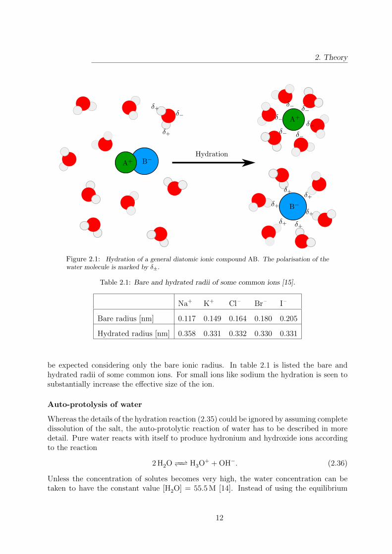
Solvation, or hydration in the common case where the solvent is water, is the process inwhich ionic compounds break up and each of the ionic species are stabilised by the solventmolecules. In figure 2.1 this process is sketched for a general diatomic ionic compoundAB in water. In reality hydration does of course happen in three dimensions and therewill be roughly one water molecule on each of the six sides of the ion.

The hydration reaction can be written as

AB(s)−−−− A m+

(aq) + B m−(aq), (2.35)

where m is the magnitude of the ionic charge. For the salts considered in this thesis theequilibrium in (2.35) lies very far to the right, and to simplify the analysis we will thereforeassume that the salt is completely dissolved at all times [14].

By forming a hydration shell around the ionic species the water molecules increasethe effective radius of the dissolved ions. This is quite important for the kinetics of ionsin a solution, as it decreases the mobility and diffusivity below the value which would

11

2. Theory

Figure 2.1: Hydration of a general diatomic ionic compound AB. The polarisation of thewater molecule is marked by δ±.

Table 2.1: Bare and hydrated radii of some common ions [15].

Na+ K+ Cl – Br – I –

Bare radius [nm] 0.117 0.149 0.164 0.180 0.205

Hydrated radius [nm] 0.358 0.331 0.332 0.330 0.331

be expected considering only the bare ionic radius. In table 2.1 is listed the bare andhydrated radii of some common ions. For small ions like sodium the hydration is seen tosubstantially increase the effective size of the ion.

Auto-protolysis of water

Whereas the details of the hydration reaction (2.35) could be ignored by assuming completedissolution of the salt, the auto-protolytic reaction of water has to be described in moredetail. Pure water reacts with itself to produce hydronium and hydroxide ions accordingto the reaction

2 H2O −−−− H3O+ + OH−. (2.36)

Unless the concentration of solutes becomes very high, the water concentration can betaken to have the constant value [H2O] = 55.5 M [14]. Instead of using the equilibrium

12

2.2. Chemical reactions

constant to describe the reaction (2.36) we can therefore use the self-ionization constantKw given as

Kw = [H3O+][OH−] = Keq[H2O] 2 ≈ 10−14 M2, (2.37)

where the last equality is valid at 300 K when the water concentration is 55.5 M. Know-ing the concentration of one of the water ions we can thus immediately calculate theconcentration of the other.

To treat systems out of equilibrium a more detailed description of the reaction, includ-ing the reaction rates, will in general be required. In this work we will however assumelocal quasi-equilibrium of the chemical reactions, which is physically justified as long asthe reactions are much faster than the transport of the reacting chemical species.

In steady-state the transport of water ions is governed by the transport equation (2.12)

∇ · JOH = R, (2.38a)

∇ · JH = R. (2.38b)

Here the subscript H is short for the hydronium ion and the reaction rates are identicalsince the reaction (2.36) produces or consumes one unit of each species. Subtracting(2.38a) from (2.38b) the unknown reaction rate is eliminated and we obtain one equationgoverning the motion of the water ions

∇ · (JH − JOH) = ∇ · Jw = 0, (2.39)

where the current density Jw ≡ JH − JOH is introduced. Since the concentrations aresimply related via the self-ionization constant, equation (2.39) together with appropriateboundary conditions is sufficient to determine the distribution of water ions.

Using the expression (2.16) for the current densities an effective Nernst-Planck equationis obtained from (2.39)

∇ ·(DH +DOHKwc

−2H

)(∇cH + cH∇φ) +

(Kwc

−2H − 1

)cHu

= 0, (2.40)

where cH is the hydronium concentration.In the remainder of this thesis cation and anion will be used to denote the positive

and negative salt ions while hydronium and hydroxide will be called by their name orcollectively referred to as water ions.

2.2.2 Surface reactions

When a solid object is brought into contact with a liquid there will usually be chemicalreactions taking place at the surface, which can leave the solid object with a surface charge.In response to this surface charge a screening layer will built up outside the surface, andthe structure of this screening layer has been an object of debate for over a century.

13

2. Theory

Helmholtz was probably the first person to give a mathematical description of thescreening layers. In his model the screening layer is viewed as an adsorbed layer of coun-terions2, making the combined surface and screening layer effectively act as a capacitor.

The model of Helmholtz makes sense only if the random thermal motion of the ionsis disregarded, as this motion will tend to move the adsorbed ions into the liquid phase.This was realised by Gouy, who suggested a rather different model for the screeninglayers, in which they are modelled as diffuse clouds of ions extending a short distanceinto the liquid. This model, known as the Gouy-Chapman model3, is the basis for muchelectrokinetic research to this day.

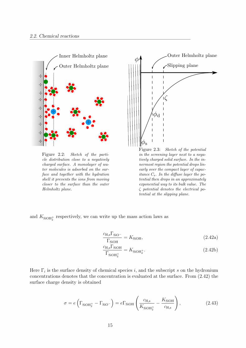
A more detailed analysis reveals that there is a limit to how close the hydrated ions canapproach the surface. This is both due to their own hydration shell and to an adsorbedmonolayer of solvent molecules on the surface. The point of closest approach of the ionsset by these constraints is denoted the outer Helmholtz plane (OHP). In contrast theinner Helmholtz plane (IHP) is defined as the locus of any ions adsorbed directly onto thesurface. In figure 2.2 is shown a sketch of the particle distribution close to a negativelycharged surface.

To model the effect of the finite approach distance, and the existence of adsorbed ions,Stern suggested combining the models of Helmholtz and Gouy, and thus view the screeninglayer as a compact layer in series with a diffuse layer. The compact layer is characterisedby the Stern capacitance Cs, which in lack of good microscopic models of the layer is oftenfound by fitting to experiments. The combined Gouy-Chapman-Stern model is currentlythe most complete model in common use and the one we shall be employing in this work.In figure 2.3 is shown a sketch of the electrical potential in the screening layer, as itis pictured in the Gouy-Chapman-Stern model. In the region closest to the surface thepotential drops linearly from its surface value φs to the value at the outer Helmholtz planeφd. In the diffuse layer the potential then drops in an approximately exponential way to itsbulk value. Also marked in the sketch is the so-called ζ-potential. The ζ potential is oftenused in electrohydrodynamics and denotes the value of the potential at the slipping plane.In this work we will assume that the slipping plane corresponds to the outer Helmholtzplane, so that the diffuse potential φd and the ζ potential are identical.

Having established the approximate structure of the screening layer, we will go on todescribe how the solid surface acquires a surface charge in the first place.

In the common case where the solid is either glass or silica, the surface charge mainlyderives from dissociation or protonation of silicon hydroxide [23, 10]

SiOH −− SiO− + H+, (2.41a)

SiOH+2−− SiOH + H+. (2.41b)

Assuming that the reactions (2.41) are in equilibrium with equilibrium constants KSiOH

2By counterions is meant ions having the opposite charge of the charged surface.3Chapman was the first to use the model of Gouy to calculate and interpret the differential capacitance

of the diffuse layer.

14

2.2. Chemical reactions

Figure 2.2: Sketch of the parti-cle distribution close to a negativelycharged surface. A monolayer of wa-ter molecules is adsorbed on the sur-face and together with the hydrationshell it prevents the ions from movingcloser to the surface than the outerHelmholtz plane.

Figure 2.3: Sketch of the potentialin the screening layer next to a nega-tively charged solid surface. In the in-nermost region the potential drops lin-early over the compact layer of capac-itance Cs. In the diffuse layer the po-tential then drops in an approximatelyexponential way to its bulk value. Theζ potential denotes the electrical po-tential at the slipping plane.

and KSiOH+2

respectively, we can write up the mass action laws as

cH,sΓSiO−

ΓSiOH

= KSiOH, (2.42a)

cH,sΓSiOH

ΓSiOH+2

= KSiOH+2. (2.42b)

Here Γi is the surface density of chemical species i, and the subscript s on the hydroniumconcentrations denotes that the concentration is evaluated at the surface. From (2.42) thesurface charge density is obtained

σ = e(

ΓSiOH+2− ΓSiO−

)= eΓSiOH

(cH,s

KSiOH+2

− KSiOH

cH,s

), (2.43)

15

2. Theory

where ΓSiOH can be related to the total surface site density Γ as

Γ = ΓSiO− + ΓSiOH + ΓSiOH+2

(2.44)

⇔ ΓSiOH = Γ

(1 +

cH,s

KSiOH+2

+KSiOH

cH,s

)−1

. (2.45)

Assuming that the hydronium is Boltzmann distributed in the compact layer, the hydro-nium concentration at the surface cH,s can be related to the concentration at the outerHelmholtz plane cH,d

cH,s = cH,de− σVTCs , (2.46)

where σCs

is the potential drop over the compact layer and VT ≡ kBTze

is the thermal voltage.The hydronium concentration at the outer Helmholtz plane cH,d does in turn depend on thepotential drop over the diffuse layer, implying that the electrostatic boundary condition(2.11) becomes highly non-linear.

16

Chapter 3

Physical Modelling

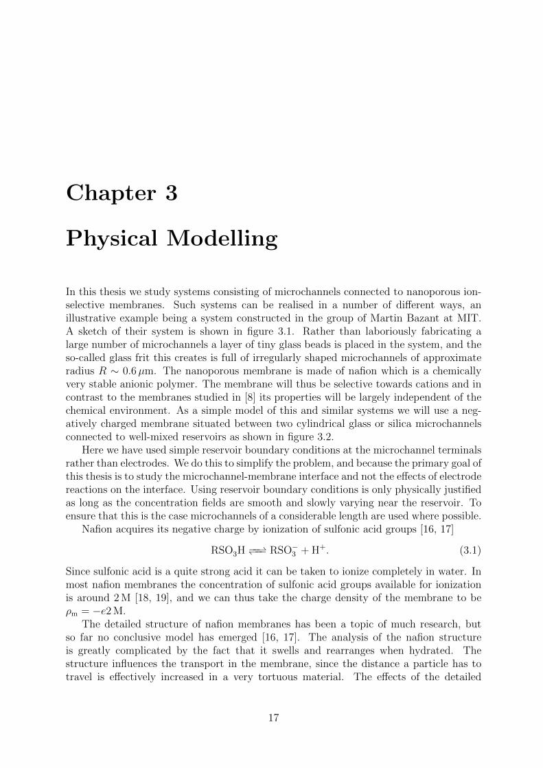
In this thesis we study systems consisting of microchannels connected to nanoporous ion-selective membranes. Such systems can be realised in a number of different ways, anillustrative example being a system constructed in the group of Martin Bazant at MIT.A sketch of their system is shown in figure 3.1. Rather than laboriously fabricating alarge number of microchannels a layer of tiny glass beads is placed in the system, and theso-called glass frit this creates is full of irregularly shaped microchannels of approximateradius R ∼ 0.6µm. The nanoporous membrane is made of nafion which is a chemicallyvery stable anionic polymer. The membrane will thus be selective towards cations and incontrast to the membranes studied in [8] its properties will be largely independent of thechemical environment. As a simple model of this and similar systems we will use a neg-atively charged membrane situated between two cylindrical glass or silica microchannelsconnected to well-mixed reservoirs as shown in figure 3.2.

Here we have used simple reservoir boundary conditions at the microchannel terminalsrather than electrodes. We do this to simplify the problem, and because the primary goal ofthis thesis is to study the microchannel-membrane interface and not the effects of electrodereactions on the interface. Using reservoir boundary conditions is only physically justifiedas long as the concentration fields are smooth and slowly varying near the reservoir. Toensure that this is the case microchannels of a considerable length are used where possible.

Nafion acquires its negative charge by ionization of sulfonic acid groups [16, 17]

RSO3H −−−− RSO−3 + H+. (3.1)

Since sulfonic acid is a quite strong acid it can be taken to ionize completely in water. Inmost nafion membranes the concentration of sulfonic acid groups available for ionizationis around 2 M [18, 19], and we can thus take the charge density of the membrane to beρm = −e2 M.

The detailed structure of nafion membranes has been a topic of much research, butso far no conclusive model has emerged [16, 17]. The analysis of the nafion structureis greatly complicated by the fact that it swells and rearranges when hydrated. Thestructure influences the transport in the membrane, since the distance a particle has totravel is effectively increased in a very tortuous material. The effects of the detailed

17

3. Physical Modelling

Figure 3.1: Sketch (not to scale) of a system including microchannels and an ion-selectivemembrane constructed in the group of Martin Bazant. The pore size of the glass frit roughlycorresponds to a radius of 0.6µm.

nafion structure are not part of this study, so we will let the membrane porosity be fixedat the typical membrane value εP = 0.4 [20] and estimate the tortuosity from the simpleexpression [21]

τ =(2− εP)2

εP. (3.2)

As the structure will primarily affect the very low voltage drop inside the membrane, theresults obtained using these estimates are expected to be of reasonable generality. From[22] the dielectric constant of dry nafion is given as εnafion ≈ 3.5. Assuming that a linearcombination of the dielectric constants of nafion and water gives a good estimate of thedielectric constant of the hydrated membrane, we then have εm = εPεw+(1−εP)εnafion ≈ 33.

Because of the nanometer pore size of the nafion membrane we expect the fluid velocityto nearly vanish inside the membrane. We will therefore assume that advection has anegligible influence in the membrane, and for the microchannel flow we will use a no slipboundary condition on the membrane surface.

For the reactions on the surface of the glass/silica microchannels we use the equilibriumconstants [23] KSiOH = 10−6.8M and KSiOH+

2= 101.9M. The total surface site density is

set to [24] Γ = 8 nm−2 and we use the value Cs = 2.9 F/m2 for the Stern capacitance [23].We investigate the case where the dissolved salt is sodium chloride, so the salt ion dif-

fusivities are given as D+ = DNa+ = 1.33× 10−9 m2/s and D− = DCl− = 2.08× 10−9 m2/s[25]. The diffusivities of the water ions are also given in [25] as DH = 9.31× 10−9 m2/s,DOH = 5.30× 10−9 m2/s.

18

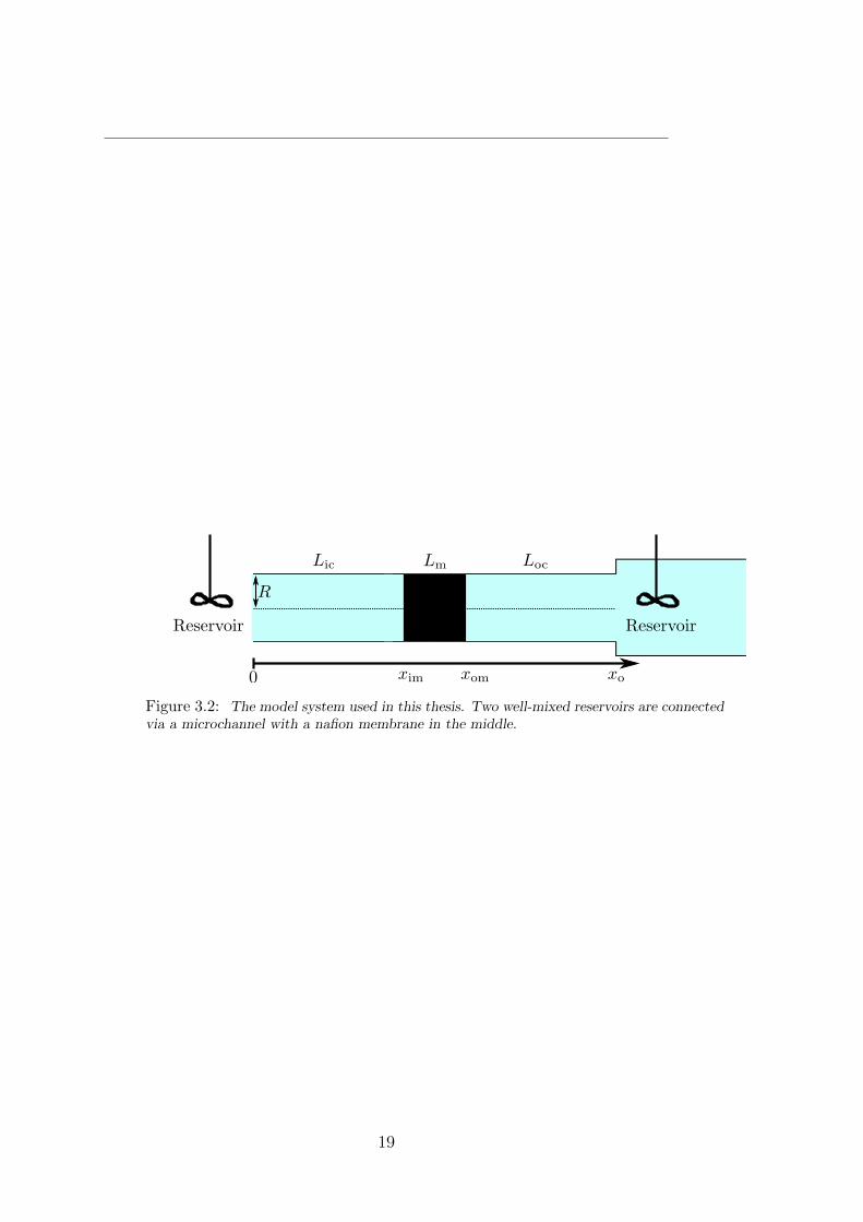
Figure 3.2: The model system used in this thesis. Two well-mixed reservoirs are connectedvia a microchannel with a nafion membrane in the middle.

19

Chapter 4

Analytical Modelling

To aid our physical understanding of electrokinetic systems some simple analytical resultsare presented in this chapter.

4.1 The diffuse part of the screening layer

We consider a simple system consisting of an infinite translationally invariant plane ofsurface charge density σ next to a liquid with two dissolved ionic species c± of oppositecharge ±ze. In equilibrium the behaviour of the diffuse part of the screening layer can befound from the field equations derived in chapter 2.

Requiring that the current densities (2.16) vanish we obtain

J± = −D±∇c± ∓ c±ze

kBTD±∇φ = 0 (4.1)

⇒ c± = c0e∓φ/VT , (4.2)

where c0 is the concentration far away from the wall where the potential is zero. For futureconvenience a normalised potential φ ≡ φ/VT is defined.

Inserting the concentrations in Gauss’s law (2.9) we arrive at the Poisson-Boltzmannequation

∇ · (−ε∇φ) = −2zec0 sinh(φ). (4.3)

Assuming that the permittivity has a constant value equal to that of pure water εw theabove equation can be rewritten

∇2φ =1

λ2D

sinh(φ), (4.4)

where the Debye length is defined as

λD ≡√εwVT

2zec0

. (4.5)

20

4.2. Overlimiting current in a microchannel

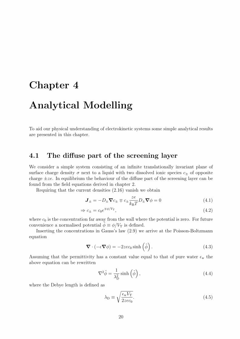
Figure 4.1: The potential in the diffuse part of the screening layer obtained from theGouy-Chapman solution. For large ζ potentials the characteristic length of the diffuse layeris seen to be significantly smaller than the Debye length.

For monovalent ions in a typical concentration of 1 mM the Debye length is around 10 nm.In the limit of low potentials (the Debye-Huckel limit) equation (4.4) can be linearised,

and the Debye length is seen to be a characteristic size of the screening layer. For largerpotentials the characteristic size of the screening layer can however be significantly smallerthan the Debye length.

In the effectively one dimensional problem of an infinite plane, equation (4.4) is inte-grable and has the Gouy-Chapman solution

φ = 4VT tanh−1

[tanh

(ζ

4VT

)e− xλD

], (4.6)

where x is the distance from the plane. The potential ζ at the outer Helmholtz plane canbe related to the surface charge density through the Grahame relation1

σ = 2VTεwλD

sinh

(ζ

2VT

). (4.7)

In figure 4.1 the potential in the diffuse layer is plotted for different values of the ζpotential. For large potentials the characteristic length of the diffuse layer is seen to bemuch smaller than the Debye length.

4.2 Overlimiting current in a microchannel

In narrow microchannels with nanoporous ion-selective membranes a reasonably accurateexpression for the overlimiting current can be found analytically.

1The Grahame relation is found by integrating (4.4) once.

21

4. Analytical Modelling

What normally complicates the analysis of overlimiting current is the extended spacecharge region, which develops in front of the ion-selective membrane. In the case at handthe majority of the charge in a cross-section of the microchannel will however stem fromthe screening layers, and it is thus a decent approximation to neglect the space chargeregion and assume electroneutrality in the bulk liquid. In the case of two ionic species c±of opposite charge ±ze the cross-sectional averages of the concentrations will therefore berelated as

ze (〈c+〉 − 〈c−〉) + 2σ

R= 0, (4.8)

for a cylindrical microchannel of radius R.Because the microchannel is narrow advection will only give a negligible contribution

to the current densities, and the average current densities become

〈J+〉 = −D+∂x 〈c+〉 −D+ 〈c+〉 ∂xφ, (4.9a)

〈J−〉 = −D−∂x 〈c−〉+D− 〈c−〉 ∂xφ = 0. (4.9b)

The last equality is valid in steady-state, where the cation selective membrane preventsan anion current from running in the system. Equation (4.9b) is easily integrated to give

〈c−〉 = c0eφ−V0 , where c0 is the inlet concentration and V0 is the normalised inlet voltage.

Using (4.8) the result can be inserted in (4.9a) to give

〈J+〉 = −D+∂x

(c0e

φ−V0 − 2 σzeR

)−D+

(c0e

φ−V0 − 2 σzeR

)∂xφ. (4.10)

Assuming constant or slowly varying surface charge density and using that the averagecurrent density is constant the above equation can be integrated once

〈J+〉D+

x = 2c0

(1− eφ−V0

)+ 2

σ

zeR(φ− V0). (4.11)

At the membrane (x = Lic) the potential is V1 so the current-voltage characteristic becomes

〈J+〉D+

Lic = 2c0

(1− eV1−V0

)+ 2

σ

zeR(V1 − V0). (4.12)

The first term on the left hand side saturates above a few thermal voltages and is re-sponsible for the classical limiting current. The second term gives a constant differentialconductance in the overlimiting regime.

The above analysis is due to Dydek et al. [9].Because the potential V1 in front of the membrane is a dependent variable, it is im-

practical to let it be a parameter in the solution (4.12). We will therefore extend theabove analysis to include the potential drop over the membrane.

In the membrane screening layers the diffusive and electromigrative currents are in op-posite directions and very large compared to the total current. The particle distribution

22

4.2. Overlimiting current in a microchannel

within the screening layers can thus to good approximation be found by simply balanc-ing the diffusive and electromigrative currents. i.e. the concentrations just outside themembrane can be related to the concentration just inside the membrane via a Boltzmannfactor. Assuming charge neutrality in the membrane, the change in potential ∆V fromoutside to inside the membrane can therefore be found by solving

εPze(c′+e

−∆V − c′−e∆V)− eNm = 0, (4.13)

where c′± are the concentrations just outside the membrane, εP is the membrane porosityand Nm is the density of negative charges in the membrane. In a perfectly selectivemembrane the anion concentration vanishes inside the membrane and we find the potentialchange as

∆V = − ln

(Nm

c′+zεP

). (4.14)

Inside the membrane the cation concentration is constant c+,m = Nm

zεPand due to elec-

troneutrality the electric field is also constant Em = −∆VmLm

. The cation current in themembrane is therefore

J+ = −frD+Nm

zεP

∆Vm

Lm

, (4.15)

where fr = εP/τ is a hindrance factor which accounts for the effects of porosity andtortuosity on the ion transport. The potential change from one end of the membrane tothe other is then

∆Vm = − J+

D+

τLmz

Nm

(4.16)

On the right hand side of the membrane the expression relating voltage and current (4.12)takes the form

〈J+〉D+

(x− xo) = 2c0

(1− eφ

)+ 2

σ

zeRφ, (4.17)

where c0 is the concentration of the outlet reservoir which is at zero potential. Just to theright of the membrane the potential is V2 and the above expression gives

〈J+〉D+

(−Loc) = 2c0

(1− eV2

)+ 2

σ

zeRV2. (4.18)

The total change in potential over the system can be written

V0 = (V1 − V0) + ∆V1 + ∆Vm −∆V2 + (0− V2), (4.19)

23

4. Analytical Modelling

where ∆V1,2 are the potential changes over the left and right membrane interfaces respec-tively.The equations (4.12) and (4.18) can be solved for the potentials and after some math acurrent-voltage relationship is obtained from (4.19)

V0 =I+Rres(Lic + Loc) + I+Rres,mLm + ln

[2 + W (2δ exp (2δ + I+RresLoc))

2 + W (2δ exp (2δ − I+RresLic))

]+ W (2δ exp (2δ − I+LicRres))−W (2δ exp (2δ + I+LocRres)) , (4.20)

where δ ≡ − c0zeR2σ

is the inlet number of ions in the bulk divided by the number of ions inthe screening layer. Rres ≡ − 1

D+2πRσis the ohmic resistance of the cations in the screening

layer and Rres,m ≡ τD+eπR2Nm

is the ohmic resistance of the cations in the membrane.

The Lambert W function solves W(x)eW(x) = x, and for positive arguments it is amonotonously increasing sublinear function.

The first and second terms in (4.20) are the ohmic voltage drops over the screeninglayers and the membrane respectively. The third term is the voltage drop over the twomembrane interfaces and the fourth and fifth terms are the voltage drops over the bulk ofthe microchannels.

In section 6.3.2 this current voltage relationship is plotted and compared to resultsfrom a more elaborate numerical model.

4.3 Dynamic surface charge density

As seen above, the magnitude of the surface charge density is the key determinant of theoverlimiting current in a microchannel. To get a feel for how the surface charge densitydepends on the physical parameters we will derive an approximate expression for it. Inthis derivation only the reaction (2.41a) is taken into account, as it will dominate for mostrealistic parameter values. Furthermore, it is used that only a small fraction of the surfacesites react so that ΓSiOH is well approximated by Γ. The surface charge density is thenapproximately given as

σ = −eΓKSiOH

cH,s

. (4.21)

In equilibrium the hydronium concentration in the screening layer is Boltzmann dis-tributed, so the concentration at the surface can be written as

cH,s = cH,bulk exp

(−ζ − σ

VTCs

). (4.22)

24

4.4. Hydronium distribution

From the Grahame relation (4.7) we have

e−ζ = exp

(−2 sinh−1

(λDσ

2εwVT

))=

( λDσ

2εwVT

)+

√1 +

(λDσ

2εwVT

)2−2

(4.23)

≈

(λDσεwVT

)2

, for ζ > 1

exp(− λDσεwVT

), for ζ < 1

. (4.24)

Inserting these expressions in (4.21) and solving for σ we find

σ ≈

−3CsVTW

(εwλD

3Cs

[eΓKSiOH

cH,bulkVTεwλD

]1/3), for ζ > 1

− VTλDεw

+ 1Cs

W(eΓKSiOH

cH,bulkVT

[λDεw

+ 1Cs

]), for ζ < 1

. (4.25)

From the expressions (4.25) it is seen that the magnitude of σ decreases monotonicallywith both the bulk hydronium concentration and the Debye length. Since the Debyelength scales as λD ∼ I−1/2, where I is the ionic strength, we expect the magnitude ofσ to increase monotonically with the salt concentration. In section 6.3.3 these trends areverified using numerical calculations.

In section 4.2 it was found that the bulk salt concentration depletes to the left of themembrane. Based only on the salt concentration we would thus expect the magnitude ofthe surface charge density to be very low in that region. Before making that prediction itis however necessary to know how the hydronium is distributed.

4.4 Hydronium distribution

The distribution of hydronium ions is unfortunately not easy to predict. The governingequation (2.40)

∇ ·(DH +DOHKwc

−2H

)(∇cH + cH∇φ) +

(Kwc

−2H − 1

)cHu

= 0, (4.26)

is highly nonlinear and even in the simple 1D case without advection it is not integrable.Let us, as a starting point, consider the case where there are no salt ions in the

system and the current is only carried by hydronium (and hydroxide). Because of thereaction term in (2.38) the hydronium ions are not conserved, and the system behaves ina fundamentally different way than the system where only salt ions are present.

In the problem where only salt ions are present the depletion and accumulation of ionsat either side of the membrane is caused by the inability of the anions to pass throughthe membrane. In the case of hydronium and hydroxide the response to any beginningdepletion or accumulation of ions will be a reaction that either creates or consumes water

25

4. Analytical Modelling

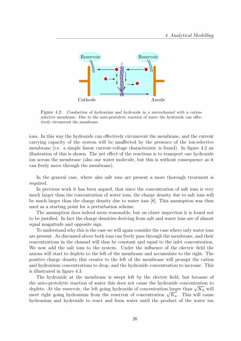
Figure 4.2: Conduction of hydronium and hydroxide in a microchannel with a cation-selective membrane. Due to the auto-protolytic reaction of water the hydroxide can effec-tively circumvent the membrane.

ions. In this way the hydroxide can effectively circumvent the membrane, and the currentcarrying capacity of the system will be unaffected by the presence of the ion-selectivemembrane (i.e. a simple linear current-voltage characteristic is found). In figure 4.2 anillustration of this is shown. The net effect of the reactions is to transport one hydroxideion across the membrane (also one water molecule, but this is without consequence as itcan freely move through the membrane).

In the general case, where also salt ions are present a more thorough treatment isrequired.

In previous work it has been argued, that since the concentration of salt ions is verymuch larger than the concentration of water ions, the charge density due to salt ions willbe much larger than the charge density due to water ions [8]. This assumption was thenused as a starting point for a perturbation scheme.

The assumption does indeed seem reasonable, but on closer inspection it is found notto be justified. In fact the charge densities deriving from salt and water ions are of almostequal magnitude and opposite sign.

To understand why this is the case we will again consider the case where only water ionsare present. As discussed above both ions can freely pass through the membrane, and theirconcentrations in the channel will thus be constant and equal to the inlet concentration.We now add the salt ions to the system. Under the influence of the electric field theanions will start to deplete to the left of the membrane and accumulate to the right. Thepositive charge density this creates to the left of the membrane will prompt the cationand hydronium concentrations to drop, and the hydroxide concentration to increase. Thisis illustrated in figure 4.3.

The hydroxide at the membrane is swept left by the electric field, but because ofthe auto-protolytic reaction of water this does not cause the hydroxide concentration todeplete. At the reservoir, the left going hydroxide of concentration larger than

√Kw will

meet right going hydronium from the reservoir of concentration√Kw. This will cause

hydronium and hydroxide to react and form water until the product of the water ion

26

4.4. Hydronium distribution

Figure 4.3: Sketch of the channel to the left of the membrane. a) Only water ions are presentin the system. Because the hydroxide (yellow) can effectively circumvent the membrane thereis no depletion region and the hydronium (red) and hydroxide concentrations are constantthrough the channel. b) Salt ions are added. The anion (blue) concentration starts to depleteand electrostatic forces affect the cations (green) and the water ions. c) The remaining ionconcentrations have been adapted to nearly satisfy electroneutrality.

Figure 4.4: The hydroxide created at the membrane is swept left by the electric field. Nearthe reservoir it reacts with hydronium to form water. The net result of these reactions isto transport one hydronium molecule from reservoir to membrane without going throughthe channel (also some water is moved). The resulting concentration curves for hydroxide(yellow) and hydronium (red) are shown.

concentrations is Kw. The result of these steps is that the depletion of hydronium andthe accumulation of hydroxide is broadened out to extend over most of the channel. Infigure 4.4 a sketch of the relevant reactions and the resulting profiles is seen.

Since the hydroxide concentration is much larger than the hydronium concentrationin most of the left channel, the water ions will contribute a significant negative spacecharge density in this region. This allows the cation concentration to be significantlylarger than zero, and the cations will thus be able to carry a current even after the anionshave depleted.

To sum up, the water ions increase the current in the system in two ways: By carryinga current themselves, and by creating a negative space charge density which allows ahigher cation concentration and thus a higher cation current.

The latter of these effects was first predicted by Kharkats and is often called the exal-tation effect [5, 7].

27

4. Analytical Modelling

Before concluding this section we briefly return to the surface charge density. Theoutcome of the above analysis was that the hydronium concentration is predicted to belowered in the left microchannel. According to (4.25) this should lead to an increase in thesurface charge density. This is opposite to the tendency predicted from the salt ions alone,and as we cannot quantify the lowering of the hydronium concentration we are at a lossas to which mechanism will dominate. We can therefore only conclude that the surfacecharge density will vary in some way in the microchannel, and then resort to numericalcalculations for the details of these variations.

28

Chapter 5

Numerical Modelling

The problems studied in this thesis are in general too complicated to allow for analyticalsolutions, and we will therefore resort to a numerical solution scheme known as the finiteelement method (FEM). The calculations are carried out in Comsol Multiphysics(Version 4.2), which is a commercially available FEM software.

5.1 The finite element method

The core idea in the finite element method is to discretise the problem by expanding thephysical fields in a set of localised basis functions1. The concept of using basis functionsin the study of boundary value problems is familiar from Fourier analysis, where harmonicfunctions are used as a basis on high symmetry geometries like rectangles, cylinders andspheres.

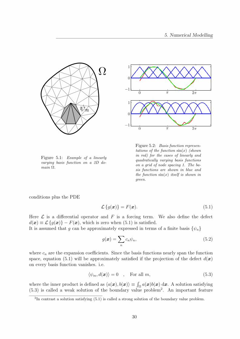
In the finite element method the basis functions are constructed by placing a grid overthe computational domain and associating a localised function with each grid node. Thevalue of the basis functions vary in some specified (usually polynomial) way between 1 attheir own node and 0 on the neighbouring nodes. This is illustrated in figure 5.1 where alinearly varying basis function on the domain Ω is shown.

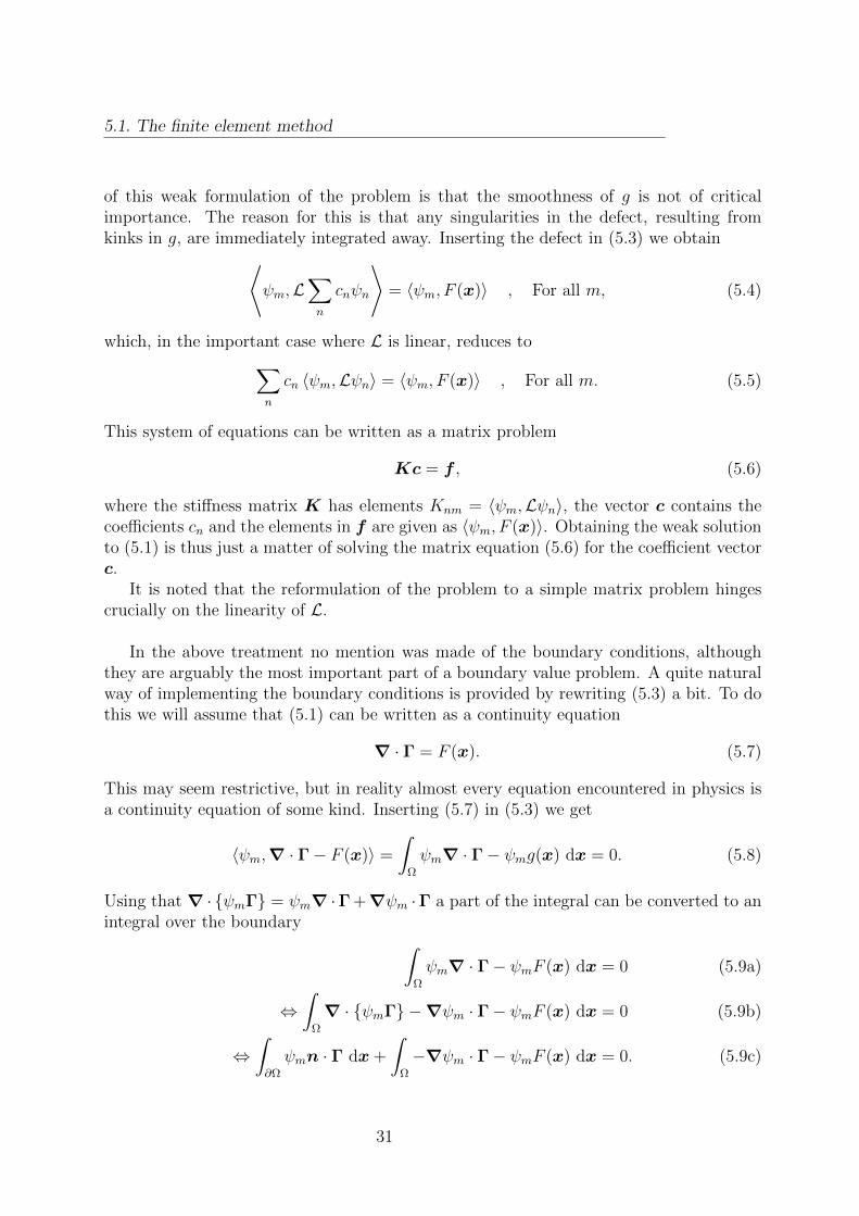
The way in which functions are represented using basis functions is most easily illus-trated in 1D. In figure 5.2 the function sin(x) is shown, together with its basis functionrepresentation, for the cases of linearly and quadratically varying basis functions on agrid of node spacing 1. It is noted that the representation of sin(x) has discontinuousderivatives at the nodes. In a classical picture this would pose a problem for the solu-tion of higher order differential equations, but as we shall later see this issue is elegantlyresolved in the finite element approach. The material in this section is based on [26, 27, 28].

We consider an inhomogeneous boundary value problem, defined by a set of boundary

1Often called test functions in the finite element method.

29

5. Numerical Modelling

Figure 5.1: Example of a linearlyvarying basis function on a 2D do-main Ω.

Figure 5.2: Basis function represen-tations of the function sin(x) (shownin red) for the cases of linearly andquadratically varying basis functionson a grid of node spacing 1. The ba-sis functions are shown in blue andthe function sin(x) itself is shown ingreen.

conditions plus the PDE

Lg(x) = F (x). (5.1)

Here L is a differential operator and F is a forcing term. We also define the defectd(x) ≡ Lg(x) − F (x), which is zero when (5.1) is satisfied.It is assumed that g can be approximately expressed in terms of a finite basis ψn

g(x) =∑n

cnψn, (5.2)

where cn are the expansion coefficients. Since the basis functions nearly span the functionspace, equation (5.1) will be approximately satisfied if the projection of the defect d(x)on every basis function vanishes. i.e.

〈ψm, d(x)〉 = 0 , For all m, (5.3)

where the inner product is defined as 〈a(x), b(x)〉 ≡∫

Ωa(x)b(x) dx. A solution satisfying

(5.3) is called a weak solution of the boundary value problem2. An important feature

2In contrast a solution satisfying (5.1) is called a strong solution of the boundary value problem.

30

5.1. The finite element method

of this weak formulation of the problem is that the smoothness of g is not of criticalimportance. The reason for this is that any singularities in the defect, resulting fromkinks in g, are immediately integrated away. Inserting the defect in (5.3) we obtain⟨

ψm,L∑n

cnψn

⟩= 〈ψm, F (x)〉 , For all m, (5.4)

which, in the important case where L is linear, reduces to∑n

cn 〈ψm,Lψn〉 = 〈ψm, F (x)〉 , For all m. (5.5)

This system of equations can be written as a matrix problem

Kc = f , (5.6)

where the stiffness matrix K has elements Knm = 〈ψm,Lψn〉, the vector c contains thecoefficients cn and the elements in f are given as 〈ψm, F (x)〉. Obtaining the weak solutionto (5.1) is thus just a matter of solving the matrix equation (5.6) for the coefficient vectorc.

It is noted that the reformulation of the problem to a simple matrix problem hingescrucially on the linearity of L.

In the above treatment no mention was made of the boundary conditions, althoughthey are arguably the most important part of a boundary value problem. A quite naturalway of implementing the boundary conditions is provided by rewriting (5.3) a bit. To dothis we will assume that (5.1) can be written as a continuity equation

∇ · Γ = F (x). (5.7)

This may seem restrictive, but in reality almost every equation encountered in physics isa continuity equation of some kind. Inserting (5.7) in (5.3) we get

〈ψm,∇ · Γ− F (x)〉 =

∫Ω

ψm∇ · Γ− ψmg(x) dx = 0. (5.8)

Using that ∇ · ψmΓ = ψm∇ ·Γ +∇ψm ·Γ a part of the integral can be converted to anintegral over the boundary ∫

Ω

ψm∇ · Γ− ψmF (x) dx = 0 (5.9a)

⇔∫

Ω

∇ · ψmΓ −∇ψm · Γ− ψmF (x) dx = 0 (5.9b)

⇔∫∂Ω

ψmn · Γ dx+

∫Ω

−∇ψm · Γ− ψmF (x) dx = 0. (5.9c)

31

5. Numerical Modelling

In (5.9c) Neumann boundary conditions can simply be implemented by replacing n ·Γ inthe surface integral with the appropriate condition. Another advantage of the formulationin (5.9c) is that it does not include derivatives of Γ, and as a consequence shape functionsof a lower order can be used to construct the basis functions.

Typically, a boundary value problem will also include Dirichlet boundary conditions.Dirichlet conditions can be considered as equations of constraint on the dependent vari-ables and written as

M = 0, (5.10)

where M depends on the dependent variables. We multiply the equation of constraint witha Lagrangian multiplier λ, and after a bit of math3 a modified version of the governingequation is obtained

∇ · Γ = F (x) +∑i

∑n

λ∂M

∂ci,n. (5.11)

Here ci,n is the coefficient to the n’th basis function of the i’th dependent variable. In thecommon case where the dependent variables enter linearly in M the constraint force justbecomes ∑

i

∑n

λ∂M

∂ci,n=∑i

∑n

λaiψi,n, (5.12)

where ai is the coefficient to the i’th dependent variable in the constraint term M .

The Lagrangian multiplier λ is a field which lives only where the constraint is defined,and it too can be expanded in a set of basis functions. The equation of constraint canthus be written

〈ψλ,m,M〉 = 0, For all m, (5.13)

where ψλ,m are the basis functions of λ. Rewriting (5.11) as done in (5.9) and adding(5.13) a single matrix problem is obtained for the solution of the boundary value problem.

As earlier noted, the approach outlined here only works for linear problems. For non-linear problems the equations are linearised around an operation point and the obtainedsolution is used to find a new operating point. This is continued until a self-consistentsolution is found.

The success of this procedure is highly dependent on the initial operating point. Whendealing with very nonlinear problems it is therefore often necessary to introduce the non-linearity slowly.

3The governing equation is treated as deriving from an unknown variational principle and the approachin [29] pp. 1065 is followed.

32

5.2. Comsol

5.2 Comsol

Comsol Multiphysics is a GUI based software implementation of the finite elementmethod. It includes diverse drawing tools for the definition of physical domains as well asa number of automated meshing sequences. Because Comsol is primarily directed towardsusers in the industry a large number of predefined physics modules are included in thesoftware. In these modules the relevant governing equations and constitutive relations forthe study of a specific physical problem are already defined, and often the user needs onlydefine the geometry and choose from a list of boundary conditions.

While convenient and fast there are a few drawbacks to using the predefined modules:When using the modules it is not always fully transparent which equations Comsolis really solving, and the modules may not be flexible enough to allow for the desiredimplementation of the physical problem.

For more flexibility and greater transparency it is possible to define the governing equa-tions and boundary conditions directly in weak form4. In this work we will be using thisoption, as a great deal of flexibility is required in the definition of some of the consideredproblems.

5.3 Mesh Convergence

The whole finite element method hinges on the assumption that the basis functions ap-proximately span the relevant function space. If this is not the case the matrix problem(5.6) might still be solvable, but the obtained solution can deviate significantly from thecorrect physical solution.

In the finite element method the ability of the basis functions to span a function spaceis determined by the coarseness of the mesh. A suitable mesh should thus be very fine inregions where the physical fields vary over small distances, while it can be quite coarsein regions with small variations of the fields. Some physical intuition about the expectedsolution can therefore greatly help in the task of defining a suitable mesh.

To verify that a given mesh is sufficiently fine to resolve the physical fields a meshconvergence test should be made. In a mesh convergence test the physical problem issolved for different meshes of varying coarseness, and a characteristic parameter obtainedfrom the solution (e.g. the current in the system) is plotted versus the coarseness. Forvery coarse meshes the mesh will have a direct effect on the problem and the chosenparameter will vary a lot when changing coarseness. As the mesh is refined the parameterwill converge towards a certain value, signifying that the mesh adequately resolves thephysical fields. The coarsest mesh giving the converged parameter value will then oftenbe chosen for the rest of the calculations. In figure 5.3 a mesh convergence plot is shown,where the mesh size is varied by scaling the chosen mesh. It is seen that the chosen mesh(scaling=1) is sufficiently refined to resolve the relevant physics.

4Also, certain types of PDE’s can be defined in coefficient form.

33

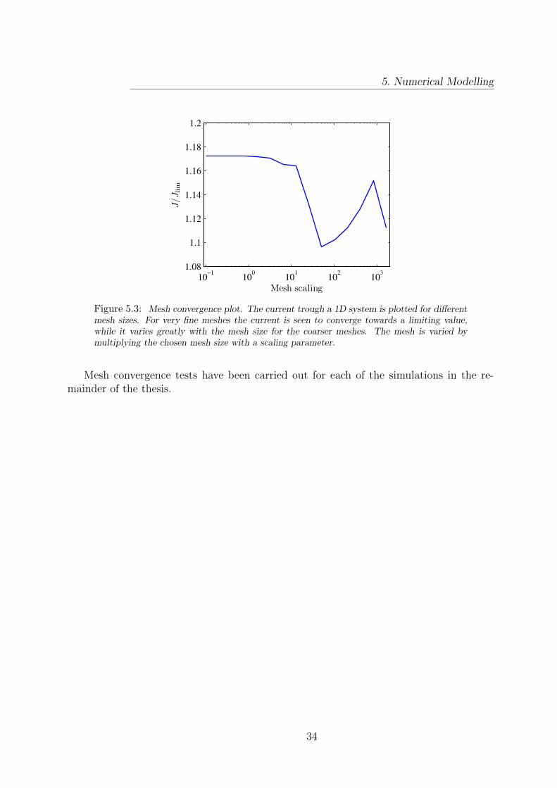
5. Numerical Modelling

Figure 5.3: Mesh convergence plot. The current trough a 1D system is plotted for differentmesh sizes. For very fine meshes the current is seen to converge towards a limiting value,while it varies greatly with the mesh size for the coarser meshes. The mesh is varied bymultiplying the chosen mesh size with a scaling parameter.

Mesh convergence tests have been carried out for each of the simulations in the re-mainder of the thesis.

34

Chapter 6

An effective 1D model for iontransport

A characteristic feature of the systems studied in this thesis is the thin screening layerswhich develop at the microchannel surfaces and at the membrane interface. The Debyelength is often taken to be the characteristic size of these screening layers, but as shownin section 4.1 the characteristic length can be orders of magnitude smaller than the Debyelength when the magnitude of the surface charge is large.

The small length scale set by the screening layers is a serious issue when meshing thephysical domains with typical dimensions R ∼ 0.5µm − 5µm and L ∼ 100µm − 1 mm.For instance it would require around 500 billion mesh elements to mesh a 5µm by 1 mmdomain with elements of side length 0.1 nm. The number of required elements can besignificantly reduced by varying the coarseness of the mesh over the domain, but thedisparate length scales set by the domain and the screening lengths do introduce a veryhigh lower limit to the number of mesh elements.

This issue motivates us to look for ways of simplifying the modelling of the physicalproblem. To this end we note that most of the complicated physics happens close to themembrane and in the extended space charge region. Outside this region it might thus bepossible to give an adequate description of the physics using a much simpler model. In thischapter we will follow this line of thought and develop a simple 1D model describing thephysics well away from the membrane and a 1D model describing the physics inside themembrane. Later we will couple these 1D models to a full 2D model near the membrane.

6.1 Modelling of the effective 1D problem

We consider a section of the microchannel which is far away from the membrane, so thatits influence is not felt directly by the salt ions or the velocity field. In the simplestcase, where the salt concentration and the surface charge density is constant along thelength of the section, this means that the current densities and the velocity field willbe unidirectional. The vanishing of the radial current density implies that the ions are

35

6. An effective 1D model for ion transport

radially equilibrated at all points in the channel section.In the general case, where the salt concentration and the surface charge density can

vary along the section, the amount of current which is carried in the bulk relative to thecurrent in the screening layers will change along the channel length. It follows that aradial current must exist. If the radial transport is much faster than the axial transportit may however still be justified to assume radial equilibrium of the ions.

Below we will use this assumption to develop a 1D model for the ion transport, andsubsequently we will estimate the regime in which the model is valid.

The electrical potential is split up in an axial part which depends only on x and anequilibrium potential which depends on both x and r.

φ(x, r) = φax(x) + φeq(x, r). (6.1)

Due to the assumption of transverse equilibrium the ion concentrations can then be writtenas

c±(x, r) = k±(x)e∓φeq(x,r), (6.2a)

cH(x, r) = h(x)e−φeq(x,r), (6.2b)

where k±(x) ≡ c±(x, 0)e±φeq(x,0) and h(x) ≡ cH(x, 0)eφeq(x,0). The Poisson equation

εw∇2φ = εw[∂2xφax +∇2φeq

]= e

[c− − c+ +

Kw

cH

− cH

], (6.3)

is split up into an axial equation

εw∂2xφax = e

(k− +

Kw

h

)− e (k+ + h) , (6.4)

and an equation for the equilibrium potential

εw∇2φeq = e

(k− +

Kw

h

)(eφeq(x,r) − 1

)− e (k+ + h)

(e−φeq(x,r) − 1

). (6.5)

Here the salt ions have been assumed monovalent.The transverse variations of φeq are much larger than the axial variations, so to a goodapproximation we can substitute ∇2φeq ≈ ∂2

rφeq + 1r∂rφeq in the above equation. The

radial and the axial problems thus only couple through k± and h.The continuity equation for the dissolved species reads

∇ · J i = ∂xJi,x +1

r∂r rJi,r = 0, (6.6)

where i ∈ +,−,w. Averaging this equation over the cross-section of the channel yieldsa continuity equation for the average axial current density

〈∇ · J i〉 = ∂x 〈Ji,x〉 = 0. (6.7)

36

6.1. Modelling of the effective 1D problem

The average axial current density is

〈J±,x〉 =D±

⟨−∂xc± ∓ c±∂x(φax + φeq)

⟩+ 〈c±u〉 (6.8)

=D±(−∂xk± ∓ k±∂xφax)⟨e∓φeq

⟩+ k±

⟨ue∓φeq

⟩, (6.9)

for the salt ions, and for the water ions it is

〈Jw,x〉 = −(DH

⟨e−φeq

⟩+DOH

Kw

h2

⟨eφeq⟩)

(∂xh+ h∂xφax) +

(h⟨ue−φeq

⟩− Kw

h

⟨ueφeq

⟩).

(6.10)

The averaged Boltzmann factors⟨e∓φeq

⟩can be found as a function of k± and h by solving

(6.5). In the following we will often use Ji as a shorthand for the average current density〈Ji〉.

In order to find the axial velocity field u we have to solve the Stokes equation. We dothis assuming unidirectionality of the flow and therefore only the axial component of theequation is considered

0 =− ∂xp+ η∇2u− ρel∂xφax

⇔ 0 =− ∂xp+ η∇2u+ εw

(∂2xφax + ∂2

xφeq +1

r∂r r∂rφeq

)(∂xφax + ∂xφeq) = 0. (6.11)

The pressure gradient term ∂xp ensures that the velocity field is incompressible whenaveraged over the cross-section. Any other purely x-dependent terms like εw∂

2xφax∂xφax

can be absorbed into the pressure gradient. Assuming that the axial variations of u andφeq are negligible equation (6.11) takes the form

∂xp =1

r∂r r∂r ηu+ εwφeq∂xφax , (6.12)

which can be integrated to give

u = −εw∂xφax

η(φeq(x, r)− ζ(x))− 1

4

∂xp

η

(R2 − r2

). (6.13)

Requiring the average velocity over the cross-section to be zero we finally get

u(x, r) = −εw∂xφax

η

[(φeq(x, r)− ζ(x))− 〈φeq(x, r)− ζ(x)〉 2

(1− r2

R2

)]. (6.14)

This expression for the velocity is separable into a part which can be found by solvingthe radial problem (the part in square brackets), and a part, ∂xφax, which pertains to theaxial problem. Introducing w ≡ − η

εw∂xφaxu the average of the velocity times the Boltzmann

factor can thus be written ⟨ueφeq

⟩= −εw∂xφax

η

⟨weφeq

⟩, (6.15)

37

6. An effective 1D model for ion transport

where the term in brackets on the right hand side can be found by solving the radialproblem (6.5).

Having reformulated the axisymmetric 3D problem into an effective 1D problem we willnow consider the range of validity of the model. The central assumption used above wasthat the radial transport happens on a much shorter time scale than the axial transport,i.e.

τr τx. (6.16)

Dimensional analysis gives that

τr ∼R2

Dand τx,1 ∼

L20

D, τx,2 ∼

L0

u0

, (6.17)

where L0 is some characteristic axial length scale and u0 is a characteristic velocity. Thereare two time scales for the axial transport since both advection and migration can beimportant. A natural choice of axial length scale is offered by scaling the derivative of therelevant concentration field

1

L0

∼ ∂xc

c= ∂x ln(c). (6.18)

The 1D model should thus be valid when

R2 L20 ⇔ R2 (∂x ln(c))2 1, (6.19)

and

R2

D∂x ln(c)u0 << 1. (6.20)

6.1.1 1D model of the membrane

Inside the membrane any transverse variations of the fields can be neglected since the poresize is of the order of nanometers. Taking the porosity εP and the permittivity εm of themembrane into account the Poisson equation therefore becomes

εm∂2xφ = εPe

(c− +

√Kw

cH

− c+ − cH

)− ρm. (6.21)

The tortuosity τ of the membrane effectively decreases the diffusivity so the current den-sities become

Ji =Di

τεP

(−∂xci ∓ ci∂xφ

), (6.22)

where i ∈ +,−,H,OH.

38

6.2. Implementation of the 1D model

6.2 Implementation of the 1D model

By construction the developed 1D model is only valid in a limited part of the system.The discrepancy between the 1D and full 2D model is however not expected to affectthe physics of the problem fundamentally, as their primary difference is that their radialdistributions differ slightly. Well aware that it will introduce an error in the results, wewill therefore attempt to model the entire system using the effective 1D model.

In the 1D model the problem is fully specified by the equations (6.4), (6.7), (6.21)and (6.22) plus appropriate boundary conditions. The average currents depend on theequilibrium potential through the average Boltzmann factors. Unfortunately, equation(6.5) is not integrable in a cylindrical geometry and it is therefore necessary to find theaverage Boltzmann factors via numerical calculations.

For a given channel radius we solve the 1D equation (6.5) on the cross-section for

different values of k± and h and tabulate the values of⟨e±φeq

⟩and

⟨we±φeq

⟩. At the

centre axis the symmetry boundary condition n ·∇φeq = 0 is used and at the channelwall the elctrostatic boundary condition εwn ·∇φeq = σ is used. Here the unit normalvector n denotes the vector pointing outwards from the domain.

The equation (6.5) only depends on k± and h through k− + Kw

hand k+ + h, so for a

constant surface charge density it is sufficient to sweep over the two parameters k− + Kw

h

and k+ + h. If, however, the dynamic surface charge density (2.43) is used a sweep overall three of the parameters k± and h is necessary.

To make⟨e±φeq

⟩and

⟨we±φeq

⟩available to Comsol as continuous and differentiable

functions Comsol is coupled to Matlab, in which the average Boltzmann factors arecubically interpolated.

The simplest way to couple the equations in the microchannels to those in the mem-brane is to simply let the expression for the space charge density and the expression forthe current density depend on position. This can be done by defining a function

f(x, a, b) =

a , For x outside the membrane

b , For x inside the membrane

. (6.23)

The current densities are then written

Ji = Dif(x,⟨e∓φeq

⟩,εPτ

)(−∂xki ∓ ki∂xφ)− f (x, 1, 0) ki

εw∂xφax

η

⟨weφeq

⟩, (6.24)

with i ∈ +,−,H,OH. Likewise, the Poisson equation becomes

∂2xφ =f

(x,

1

εw, 0

)[e

(k− +

Kw

h

)− e (k+ + h)

](6.25)

+f

(x, 0,

1

εm

)[εPe

(k− +

√Kw

h− k+ − h

)− ρm

]. (6.26)

39

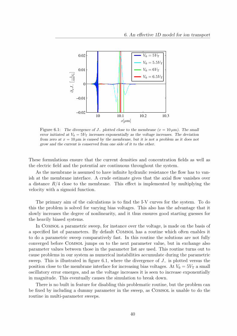
6. An effective 1D model for ion transport

Figure 6.1: The divergence of J− plotted close to the membrane (x = 10µm). The smallerror initiated at V0 = 5VT increases exponentially as the voltage increases. The deviationfrom zero at x = 10µm is caused by the membrane, but it is not a problem as it does notgrow and the current is conserved from one side of it to the other.

These formulations ensure that the current densities and concentration fields as well asthe electric field and the potential are continuous throughout the system.

As the membrane is assumed to have infinite hydraulic resistance the flow has to van-ish at the membrane interface. A crude estimate gives that the axial flow vanishes overa distance R/4 close to the membrane. This effect is implemented by multiplying thevelocity with a sigmoid function.

The primary aim of the calculations is to find the I-V curves for the system. To dothis the problem is solved for varying bias voltages. This also has the advantage that itslowly increases the degree of nonlinearity, and it thus ensures good starting guesses forthe heavily biased systems.

In Comsol a parametric sweep, for instance over the voltage, is made on the basis ofa specified list of parameters. By default Comsol has a routine which often enables itto do a parametric sweep comparatively fast. In this routine the solutions are not fullyconverged before Comsol jumps on to the next parameter value, but in exchange alsoparameter values between those in the parameter list are used. This routine turns out tocause problems in our system as numerical instabilities accumulate during the parametricsweep. This is illustrated in figure 6.1, where the divergence of J− is plotted versus theposition close to the membrane interface for increasing bias voltages. At V0 = 5VT a smalloscillatory error emerges, and as the voltage increases it is seen to increase exponentiallyin magnitude. This eventually causes the simulation to break down.

There is no built in feature for disabling this problematic routine, but the problem canbe fixed by including a dummy parameter in the sweep, as Comsol is unable to do theroutine in multi-parameter sweeps.

40

6.3. Results

6.3 Results

To be able to properly discriminate between the consequences of different physical ef-fects a number of calculations including increasingly complex physics are carried out. Insuccession we consider the cases of zero, constant and dynamic surface charge density.

6.3.1 Zero surface charge density

The case of zero surface charge actually describes a very wide channel, where surfaceeffects can be neglected, connected to a membrane. In this effectively translation invariantsystem the 1D equations exactly describe the physics (i.e. if we disregard the possibilityof symmetry breaking).

The calculations are carried out both with and without water ions included in themodel. In figure 6.2 the electric current densities are plotted for both cases. The currentsare normalised with the classical limiting current density Jlim = 2 eD+c0

Lic, c.f. equation

(4.12). The inlet concentration was taken as c0 = 1 mM, the inlet pH as 7 and the lengthswere Lic = 1 mm, Lm = 100µm and Loc = 1 mm.

Without water ions the current exceeds the classical limiting current slightly for largevoltages. This is due to the formation of an extended space charge layer in front of themembrane. To illustrate this the cation concentration and the space charge density in theleft channel have been plotted in figure 6.3.

For the case with hydronium both the cation current J+ and the total current Jtot areplotted in 6.2. The current is increased above the current in the hydronium-free systemby two effects as discussed in section 4.4. One effect is that the hydroxide can effectivelycircumvent the membrane, and a large water ion current can thus run in the system as thecurrent is only slightly hindered by the membrane. The other effect is that a larger cationcurrent can run in the system, because the cation concentration can deviate more from theanion concentration when screened by the water ions (the exaltation effect). The chargedensity deriving from water ions can be very large as seen in figure 6.5. The charge densityfrom the salt ions will however almost cancel it out, so that the total charge density (figure6.4) resembles the charge density found without water ions in the system (figure 6.3).

6.3.2 Constant surface charge density

We now go on to consider the slightly more complicated case of a microchannel withconstant, finite surface charge density. Simulations have been made for a model excludingwater ions and flow, for a model including water ions but excluding flow and for a modelincluding both flow and water ions. The resulting I-V curves are shown in figure 6.6,where also the analytical expression (4.20) is plotted for comparison. Again, the inletconcentration was taken as c0 = 1 mM, the inlet pH as 7 and the lengths were Lic = 1 mm,Lm = 100µm and Loc = 1 mm. A channel of radius R = 1µm with surface charge densityσ = 1 mC/m2 was used.

41

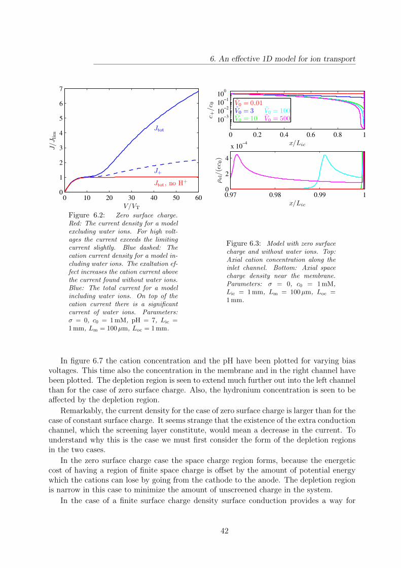
6. An effective 1D model for ion transport

Figure 6.2: Zero surface charge.Red: The current density for a modelexcluding water ions. For high volt-ages the current exceeds the limitingcurrent slightly. Blue dashed: Thecation current density for a model in-cluding water ions. The exaltation ef-fect increases the cation current abovethe current found without water ions.Blue: The total current for a modelincluding water ions. On top of thecation current there is a significantcurrent of water ions. Parameters:σ = 0, c0 = 1 mM, pH = 7, Lic =1 mm, Lm = 100µm, Loc = 1 mm.

Figure 6.3: Model with zero surfacecharge and without water ions. Top:Axial cation concentration along theinlet channel. Bottom: Axial spacecharge density near the membrane.Parameters: σ = 0, c0 = 1 mM,Lic = 1 mm, Lm = 100µm, Loc =1 mm.

In figure 6.7 the cation concentration and the pH have been plotted for varying biasvoltages. This time also the concentration in the membrane and in the right channel havebeen plotted. The depletion region is seen to extend much further out into the left channelthan for the case of zero surface charge. Also, the hydronium concentration is seen to beaffected by the depletion region.

Remarkably, the current density for the case of zero surface charge is larger than for thecase of constant surface charge. It seems strange that the existence of the extra conductionchannel, which the screening layer constitute, would mean a decrease in the current. Tounderstand why this is the case we must first consider the form of the depletion regionsin the two cases.

In the zero surface charge case the space charge region forms, because the energeticcost of having a region of finite space charge is offset by the amount of potential energywhich the cations can lose by going from the cathode to the anode. The depletion regionis narrow in this case to minimize the amount of unscreened charge in the system.

In the case of a finite surface charge density surface conduction provides a way for

42

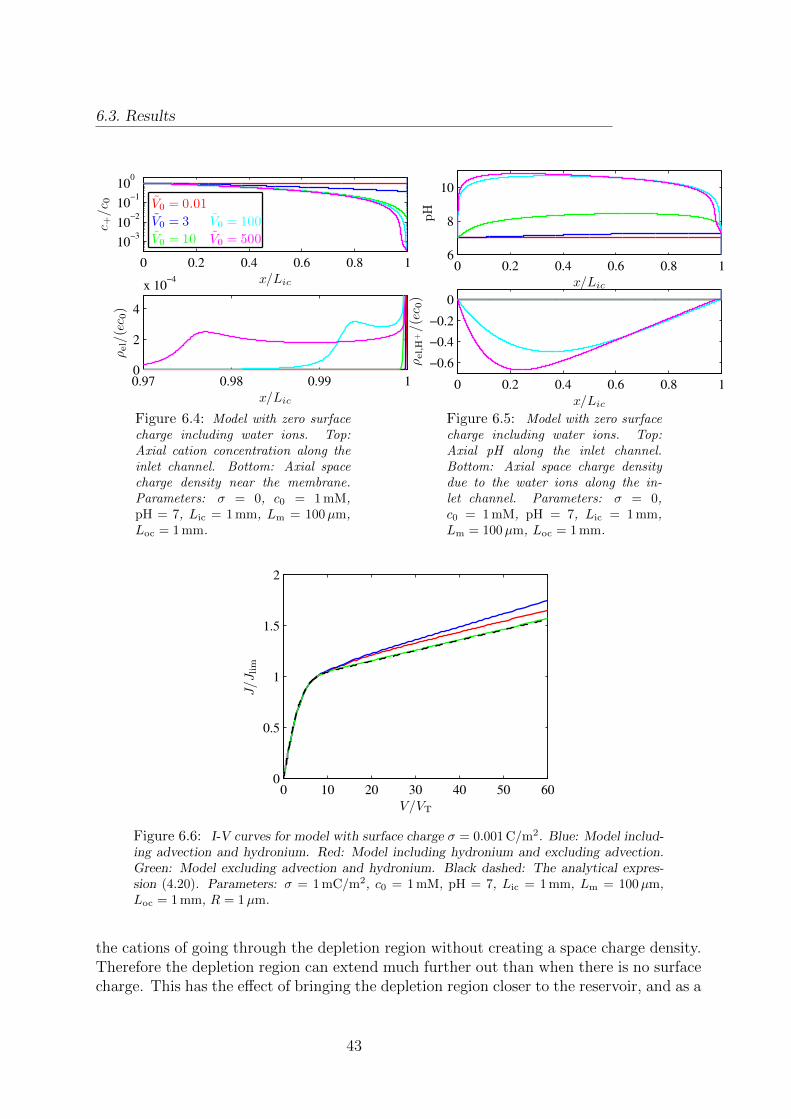
6.3. Results

Figure 6.4: Model with zero surfacecharge including water ions. Top:Axial cation concentration along theinlet channel. Bottom: Axial spacecharge density near the membrane.Parameters: σ = 0, c0 = 1 mM,pH = 7, Lic = 1 mm, Lm = 100µm,Loc = 1 mm.

Figure 6.5: Model with zero surfacecharge including water ions. Top:Axial pH along the inlet channel.Bottom: Axial space charge densitydue to the water ions along the in-let channel. Parameters: σ = 0,c0 = 1 mM, pH = 7, Lic = 1 mm,Lm = 100µm, Loc = 1 mm.

Figure 6.6: I-V curves for model with surface charge σ = 0.001 C/m2. Blue: Model includ-ing advection and hydronium. Red: Model including hydronium and excluding advection.Green: Model excluding advection and hydronium. Black dashed: The analytical expres-sion (4.20). Parameters: σ = 1 mC/m2, c0 = 1 mM, pH = 7, Lic = 1 mm, Lm = 100µm,Loc = 1 mm, R = 1µm.

the cations of going through the depletion region without creating a space charge density.Therefore the depletion region can extend much further out than when there is no surfacecharge. This has the effect of bringing the depletion region closer to the reservoir, and as a

43

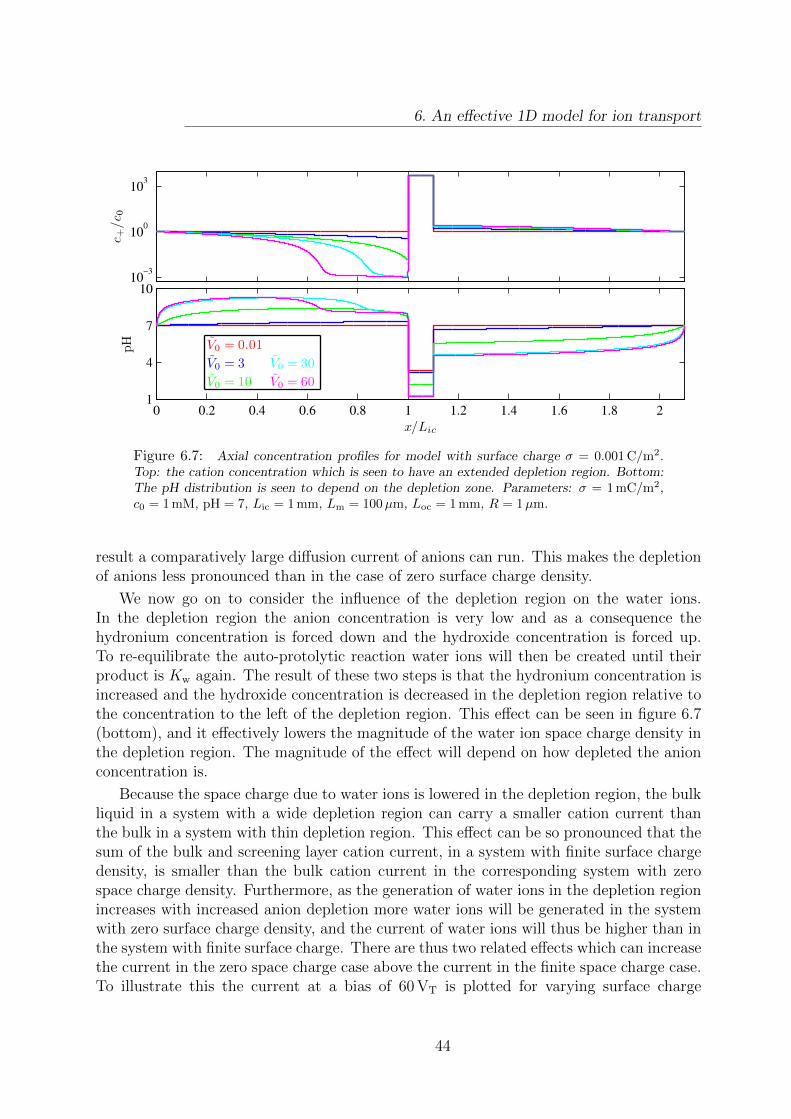
6. An effective 1D model for ion transport

Figure 6.7: Axial concentration profiles for model with surface charge σ = 0.001 C/m2.Top: the cation concentration which is seen to have an extended depletion region. Bottom:The pH distribution is seen to depend on the depletion zone. Parameters: σ = 1 mC/m2,c0 = 1 mM, pH = 7, Lic = 1 mm, Lm = 100µm, Loc = 1 mm, R = 1µm.

result a comparatively large diffusion current of anions can run. This makes the depletionof anions less pronounced than in the case of zero surface charge density.

We now go on to consider the influence of the depletion region on the water ions.In the depletion region the anion concentration is very low and as a consequence thehydronium concentration is forced down and the hydroxide concentration is forced up.To re-equilibrate the auto-protolytic reaction water ions will then be created until theirproduct is Kw again. The result of these two steps is that the hydronium concentration isincreased and the hydroxide concentration is decreased in the depletion region relative tothe concentration to the left of the depletion region. This effect can be seen in figure 6.7(bottom), and it effectively lowers the magnitude of the water ion space charge density inthe depletion region. The magnitude of the effect will depend on how depleted the anionconcentration is.

Because the space charge due to water ions is lowered in the depletion region, the bulkliquid in a system with a wide depletion region can carry a smaller cation current thanthe bulk in a system with thin depletion region. This effect can be so pronounced that thesum of the bulk and screening layer cation current, in a system with finite surface chargedensity, is smaller than the bulk cation current in the corresponding system with zerospace charge density. Furthermore, as the generation of water ions in the depletion regionincreases with increased anion depletion more water ions will be generated in the systemwith zero surface charge density, and the current of water ions will thus be higher than inthe system with finite surface charge. There are thus two related effects which can increasethe current in the zero space charge case above the current in the finite space charge case.To illustrate this the current at a bias of 60 VT is plotted for varying surface charge

44

6.3. Results

Figure 6.8: Total current density (full line) and cation current density (dashed) plotted fora bias voltage of 60 VT versus the surface charge density. Parameters: c0 = 1 mM, pH = 7,Lic = 1 mm, Lm = 100µm, Loc = 1 mm, R = 1µm.

densities in figure 6.8. A clear minimum is visible in the plot. For large surface chargedensities surface conduction dominates the current which therefore increases linearly withthe surface charge.

6.3.3 Dynamic surface charge density

In the study of the dynamic surface charge density the lengths Lic = 1 mm, Lm = 100µmand Loc = 1 mm were used again. The radius took on the valuesR = 0.2µm, R = 1µm andR = 5µm, the reservoir salt concentration was varied from c0 = 0.1 mM over c0 = 1 mMto c0 = 10 mM and the reservoir pH took on the values 5.5, 7 and 8.5.

Before presenting the I-V curves we will consider the effect of the concentration fieldson the surface charge density. In figure 6.9 the surface charge density is plotted versusthe bulk ionic strength (assuming electroneutrality) and the bulk pH for a channel ofradius R = 5µm1. As predicted in section 4.3 the magnitude of the surface charge densityincreases with both pH and ionic strength.

Because of the dynamic surface charge density the amount of ions which can be con-ducted through the screening layers depends on the bulk hydronium and salt concentra-tion. This influence is evident in the I-V curves, where the overlimiting conductance variessignificantly with the bias voltage. In figure 6.10 the total current density is plotted ina channel of radius R = 1µm for varying c0 and pH, and in figure 6.10 the current isplotted in a channel of radius R = 5µm. The currents are normalised with the limitingcurrent, so in fact the current is smaller for c0 = 1 mM than for c0 = 10 mM although theplots seem to show the opposite. The average current densities are larger for small radii

1Because the width of the screening layers is much smaller than the radius, the radius will have anegligible influence on the surface charge density.

45

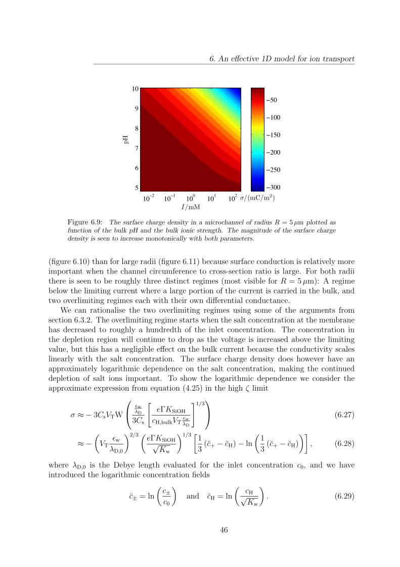
6. An effective 1D model for ion transport

Figure 6.9: The surface charge density in a microchannel of radius R = 5µm plotted asfunction of the bulk pH and the bulk ionic strength. The magnitude of the surface chargedensity is seen to increase monotonically with both parameters.

(figure 6.10) than for large radii (figure 6.11) because surface conduction is relatively moreimportant when the channel circumference to cross-section ratio is large. For both radiithere is seen to be roughly three distinct regimes (most visible for R = 5µm): A regimebelow the limiting current where a large portion of the current is carried in the bulk, andtwo overlimiting regimes each with their own differential conductance.

We can rationalise the two overlimiting regimes using some of the arguments fromsection 6.3.2. The overlimiting regime starts when the salt concentration at the membranehas decreased to roughly a hundredth of the inlet concentration. The concentration inthe depletion region will continue to drop as the voltage is increased above the limitingvalue, but this has a negligible effect on the bulk current because the conductivity scaleslinearly with the salt concentration. The surface charge density does however have anapproximately logarithmic dependence on the salt concentration, making the continueddepletion of salt ions important. To show the logarithmic dependence we consider theapproximate expression from equation (4.25) in the high ζ limit

σ ≈− 3CsVTW

εwλD

3Cs

[eΓKSiOH

cH,bulkVTεwλD

]1/3 (6.27)

≈−(VT

εwλD,0

)2/3(eΓKSiOH√

Kw

)1/3 [1

3(c+ − cH)− ln

(1

3(c+ − cH)

)], (6.28)

where λD,0 is the Debye length evaluated for the inlet concentration c0, and we haveintroduced the logarithmic concentration fields

c± = ln

(c±c0

)and cH = ln

(cH√Kw

). (6.29)

46

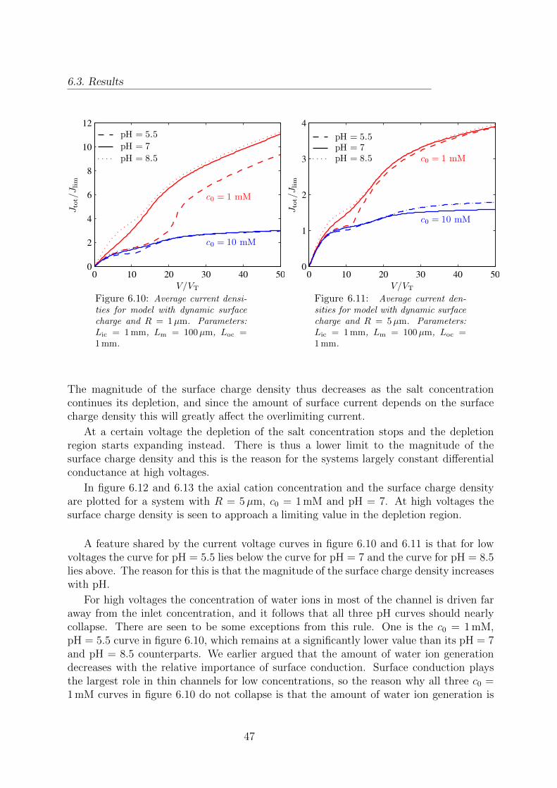
6.3. Results

Figure 6.10: Average current densi-ties for model with dynamic surfacecharge and R = 1µm. Parameters:Lic = 1 mm, Lm = 100µm, Loc =1 mm.

Figure 6.11: Average current den-sities for model with dynamic surfacecharge and R = 5µm. Parameters:Lic = 1 mm, Lm = 100µm, Loc =1 mm.

The magnitude of the surface charge density thus decreases as the salt concentrationcontinues its depletion, and since the amount of surface current depends on the surfacecharge density this will greatly affect the overlimiting current.

At a certain voltage the depletion of the salt concentration stops and the depletionregion starts expanding instead. There is thus a lower limit to the magnitude of thesurface charge density and this is the reason for the systems largely constant differentialconductance at high voltages.

In figure 6.12 and 6.13 the axial cation concentration and the surface charge densityare plotted for a system with R = 5µm, c0 = 1 mM and pH = 7. At high voltages thesurface charge density is seen to approach a limiting value in the depletion region.

A feature shared by the current voltage curves in figure 6.10 and 6.11 is that for lowvoltages the curve for pH = 5.5 lies below the curve for pH = 7 and the curve for pH = 8.5lies above. The reason for this is that the magnitude of the surface charge density increaseswith pH.

For high voltages the concentration of water ions in most of the channel is driven faraway from the inlet concentration, and it follows that all three pH curves should nearlycollapse. There are seen to be some exceptions from this rule. One is the c0 = 1 mM,pH = 5.5 curve in figure 6.10, which remains at a significantly lower value than its pH = 7and pH = 8.5 counterparts. We earlier argued that the amount of water ion generationdecreases with the relative importance of surface conduction. Surface conduction playsthe largest role in thin channels for low concentrations, so the reason why all three c0 =1 mM curves in figure 6.10 do not collapse is that the amount of water ion generation is

47

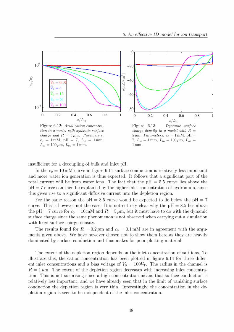
6. An effective 1D model for ion transport

Figure 6.12: Axial cation concentra-tion in a model with dynamic surfacecharge and R = 5µm. Parameters:c0 = 1 mM, pH = 7, Lic = 1 mm,Lm = 100µm, Loc = 1 mm.

Figure 6.13: Dynamic surfacecharge density in a model with R =5µm. Parameters: c0 = 1 mM, pH =7, Lic = 1 mm, Lm = 100µm, Loc =1 mm.

insufficient for a decoupling of bulk and inlet pH.

In the c0 = 10 mM curve in figure 6.11 surface conduction is relatively less importantand more water ion generation is thus expected. It follows that a significant part of thetotal current will be from water ions. The fact that the pH = 5.5 curve lies above thepH = 7 curve can then be explained by the higher inlet concentration of hydronium, sincethis gives rise to a significant diffusive current into the depletion region.

For the same reason the pH = 8.5 curve would be expected to lie below the pH = 7curve. This is however not the case. It is not entirely clear why the pH = 8.5 lies abovethe pH = 7 curve for c0 = 10 mM and R = 5µm, but it must have to do with the dynamicsurface charge since the same phenomenon is not observed when carrying out a simulationwith fixed surface charge density.

The results found for R = 0.2µm and c0 = 0.1 mM are in agreement with the argu-ments given above. We have however chosen not to show them here as they are heavilydominated by surface conduction and thus makes for poor plotting material.

The extent of the depletion region depends on the inlet concentration of salt ions. Toillustrate this, the cation concentration has been plotted in figure 6.14 for three differ-ent inlet concentrations and a bias voltage of V0 = 100VT. The radius in the channel isR = 1µm. The extent of the depletion region decreases with increasing inlet concentra-tion. This is not surprising since a high concentration means that surface conduction isrelatively less important, and we have already seen that in the limit of vanishing surfaceconduction the depletion region is very thin. Interestingly, the concentration in the de-pletion region is seen to be independent of the inlet concentration.

48

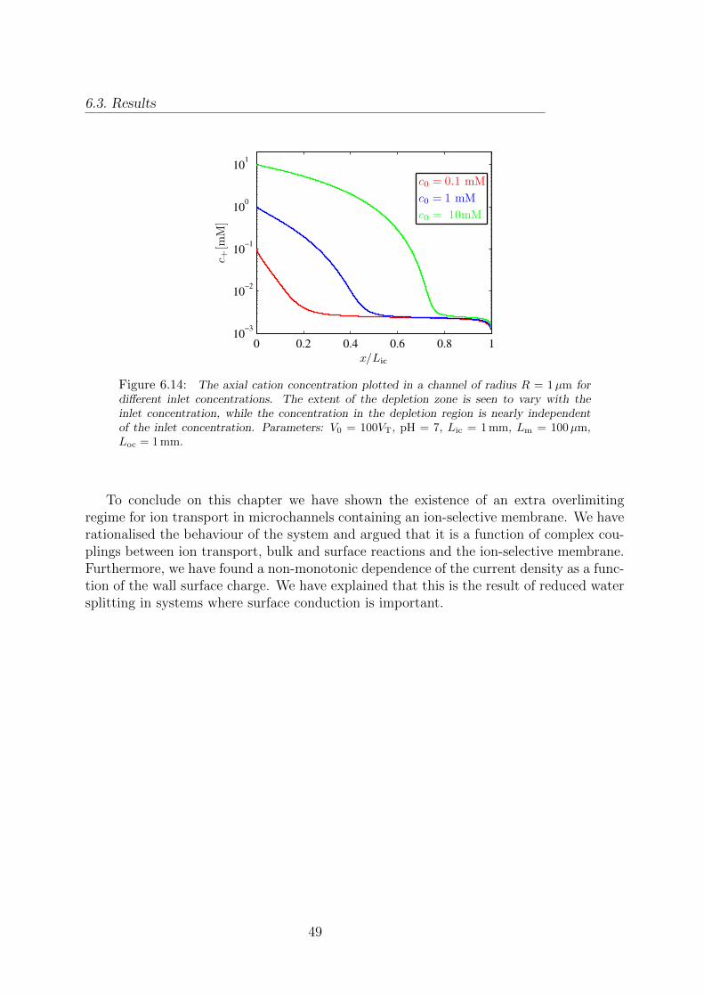
6.3. Results

Figure 6.14: The axial cation concentration plotted in a channel of radius R = 1µm fordifferent inlet concentrations. The extent of the depletion zone is seen to vary with theinlet concentration, while the concentration in the depletion region is nearly independentof the inlet concentration. Parameters: V0 = 100VT, pH = 7, Lic = 1 mm, Lm = 100µm,Loc = 1 mm.

To conclude on this chapter we have shown the existence of an extra overlimitingregime for ion transport in microchannels containing an ion-selective membrane. We haverationalised the behaviour of the system and argued that it is a function of complex cou-plings between ion transport, bulk and surface reactions and the ion-selective membrane.Furthermore, we have found a non-monotonic dependence of the current density as a func-tion of the wall surface charge. We have explained that this is the result of reduced watersplitting in systems where surface conduction is important.

49

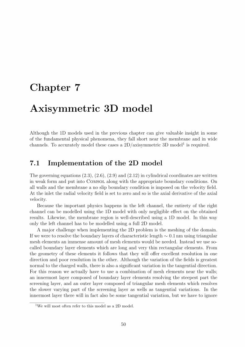
Chapter 7

Axisymmetric 3D model

Although the 1D models used in the previous chapter can give valuable insight in someof the fundamental physical phenomena, they fall short near the membrane and in widechannels. To accurately model these cases a 2D/axisymmetric 3D model1 is required.

7.1 Implementation of the 2D model

The governing equations (2.3), (2.6), (2.9) and (2.12) in cylindrical coordinates are writtenin weak form and put into Comsol along with the appropriate boundary conditions. Onall walls and the membrane a no slip boundary condition is imposed on the velocity field.At the inlet the radial velocity field is set to zero and so is the axial derivative of the axialvelocity.

Because the important physics happens in the left channel, the entirety of the rightchannel can be modelled using the 1D model with only negligible effect on the obtainedresults. Likewise, the membrane region is well-described using a 1D model. In this wayonly the left channel has to be modelled using a full 2D model.

A major challenge when implementing the 2D problem is the meshing of the domain.If we were to resolve the boundary layers of characteristic length ∼ 0.1 nm using triangularmesh elements an immense amount of mesh elements would be needed. Instead we use so-called boundary layer elements which are long and very thin rectangular elements. Fromthe geometry of these elements it follows that they will offer excellent resolution in onedirection and poor resolution in the other. Although the variation of the fields is greatestnormal to the charged walls, there is also a significant variation in the tangential direction.For this reason we actually have to use a combination of mesh elements near the walls;an innermost layer composed of boundary layer elements resolving the steepest part thescreening layer, and an outer layer composed of triangular mesh elements which resolvesthe slower varying part of the screening layer as wells as tangential variations. In theinnermost layer there will in fact also be some tangential variation, but we have to ignore

1We will most often refer to this model as a 2D model.

50

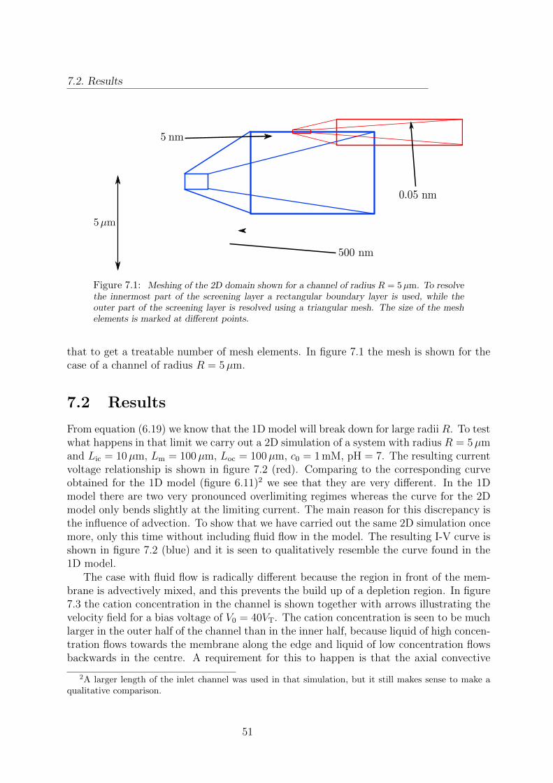
7.2. Results

Figure 7.1: Meshing of the 2D domain shown for a channel of radius R = 5µm. To resolvethe innermost part of the screening layer a rectangular boundary layer is used, while theouter part of the screening layer is resolved using a triangular mesh. The size of the meshelements is marked at different points.

that to get a treatable number of mesh elements. In figure 7.1 the mesh is shown for thecase of a channel of radius R = 5µm.

7.2 Results

From equation (6.19) we know that the 1D model will break down for large radii R. To testwhat happens in that limit we carry out a 2D simulation of a system with radius R = 5µmand Lic = 10µm, Lm = 100µm, Loc = 100µm, c0 = 1 mM, pH = 7. The resulting currentvoltage relationship is shown in figure 7.2 (red). Comparing to the corresponding curveobtained for the 1D model (figure 6.11)2 we see that they are very different. In the 1Dmodel there are two very pronounced overlimiting regimes whereas the curve for the 2Dmodel only bends slightly at the limiting current. The main reason for this discrepancy isthe influence of advection. To show that we have carried out the same 2D simulation oncemore, only this time without including fluid flow in the model. The resulting I-V curve isshown in figure 7.2 (blue) and it is seen to qualitatively resemble the curve found in the1D model.

The case with fluid flow is radically different because the region in front of the mem-brane is advectively mixed, and this prevents the build up of a depletion region. In figure7.3 the cation concentration in the channel is shown together with arrows illustrating thevelocity field for a bias voltage of V0 = 40VT. The cation concentration is seen to be muchlarger in the outer half of the channel than in the inner half, because liquid of high concen-tration flows towards the membrane along the edge and liquid of low concentration flowsbackwards in the centre. A requirement for this to happen is that the axial convective

2A larger length of the inlet channel was used in that simulation, but it still makes sense to make aqualitative comparison.

51

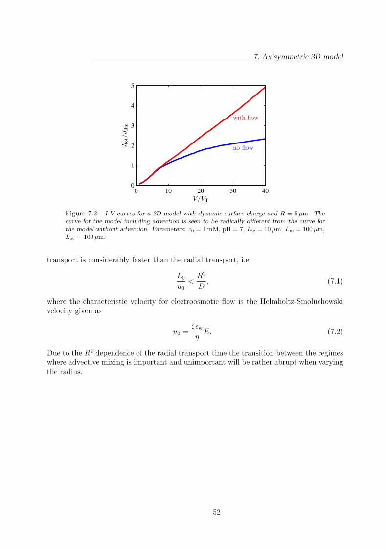
7. Axisymmetric 3D model

Figure 7.2: I-V curves for a 2D model with dynamic surface charge and R = 5µm. Thecurve for the model including advection is seen to be radically different from the curve forthe model without advection. Parameters: c0 = 1 mM, pH = 7, Lic = 10µm, Lm = 100µm,Loc = 100µm.

transport is considerably faster than the radial transport, i.e.

L0

u0

<R2

D, (7.1)

where the characteristic velocity for electroosmotic flow is the Helmholtz-Smoluchowskivelocity given as

u0 =ζεwηE. (7.2)

Due to the R2 dependence of the radial transport time the transition between the regimeswhere advective mixing is important and unimportant will be rather abrupt when varyingthe radius.

52

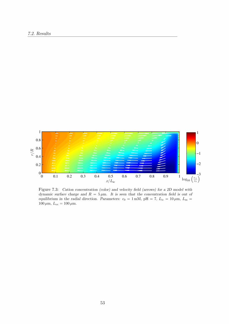
7.2. Results

Figure 7.3: Cation concentration (color) and velocity field (arrows) for a 2D model withdynamic surface charge and R = 5µm. It is seen that the concentration field is out ofequilibrium in the radial direction. Parameters: c0 = 1 mM, pH = 7, Lic = 10µm, Lm =100µm, Loc = 100µm.

53

Chapter 8

A coupled 1D-2D model for the iontransport

The computational cost of running a 2D simulation makes it inconvenient to simulate largesystems using a full 2D model. On the other hand the 1D model does not fully describethe physics close to the membrane. For channels which are not too wide the 1D modeldoes however give a good description of the region far away from the membrane. We willtherefore attempt to combine the accuracy of the 2D model with the low computationalcost of the 1D model by modelling the part of the system far from the membrane usingthe 1D model, and the part of the system close to the membrane using a 2D model.

8.1 Coupling of 1D and 2D model

The 1D model is valid when the inequality (6.19) is satisfied, and from this it follows thatthe domain of validity will depend on the extent of the depletion zone. During a voltagesweep the depletion zone expands and the point where 1D and 2D model couples shouldthus be able to move. In Comsol this means that the 1D domain should shrink and the2D domain should expand. While it is possible to sweep over geometries in Comsol, itmakes it impossible to use the previous solution as a starting guess because the remeshingof the domains introduces a new FEM basis. Due to the nonlinearity of the problem,solutions for high bias voltages require a good starting guess, i.e. it requires that theprevious solution is used as an initial condition.

We can get around this problem by scaling the spatial variables to effectively changethe domain size without having to change the geometry. Stretching the 2D domain usingscaling variables has the effect of effectively coarsening the mesh. This could be problem-atic, but conveniently the relevant physical length scale (the Debye length) expands atthe same time as the mesh is coarsened, because the salt concentration in the depletionregion becomes very low.

The inlet channel of length Lic is divided into an inlet region of length Lir, modelled

54

8.1. Coupling of 1D and 2D model

using the 1D model, and a transition region of length Ltr, modelled using the 2D model.We also introduce the unscaled lengths of the regions Lir,0 and Ltr,0. The spatial variablein the axial direction x can be related to the unscaled variable x as

x =Lir

Lir,0

x In the inlet region, (8.1a)

x = Lir +Ltr

Ltr,0

x In the transition region. (8.1b)

It proves convenient to introduce the scaling parameters

γir =Lir

Lir,0

and γtr =Ltr

Ltr,0

, (8.2)

which are related as

γtr = 1 +Lir,0

Ltr,0

(1− γir) , (8.3)

since the total length of the channel is independent of the scaling. The derivatives thentransform as

∂

∂x=

1

γα

∂

∂x, (8.4)

where α ∈ ir, tr.Let us now consider how the scaling affects the governing equations and boundary

conditions. To do that we consider the general PDE

∇ · Γ = F (x), (8.5)

which, as shown in section 5.1, can be rewritten in weak form∫∂Ω

ψmn · Γ dx+

∫Ω

−∇ψm · Γ− ψmF (x) dx = 0. (8.6)

When scaled, any derivatives appearing in Γ and F (x) should be modified according to(8.4). In a cylindrical geometry the volume integral becomes∫

Ω

−∇ψm · Γ− ψmF dx =

∫Ω

2πr [−∂rψmΓr − ∂xψmΓx − ψmF ] drdx (8.7)

=

∫Ω

2πr

[−∂rψmΓr −

1

γα∂xψmΓx − ψmF

]γα drdx, (8.8)

and the surface integral becomes∫∂Ω

ψmn · Γ dx =

∫∂Ω

2πr [ψmnxΓx + ψmγαnrΓr] drdx. (8.9)

At the point where 1D and 2D model couples continuity of Γ and the dependent variablesis required.

55

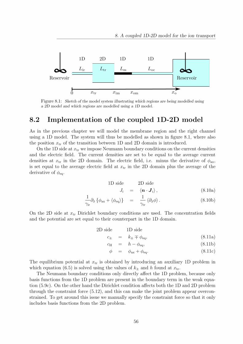
8. A coupled 1D-2D model for the ion transport

Figure 8.1: Sketch of the model system illustrating which regions are being modelled usinga 2D model and which regions are modelled using a 1D model.

8.2 Implementation of the coupled 1D-2D model

As in the previous chapter we will model the membrane region and the right channelusing a 1D model. The system will thus be modelled as shown in figure 8.1, where alsothe position xtr of the transition between 1D and 2D domain is introduced.

On the 1D side at xtr we impose Neumann boundary conditions on the current densitiesand the electric field. The current densities are set to be equal to the average currentdensities at xtr in the 2D domain. The electric field, i.e. minus the derivative of φax,is set equal to the average electric field at xtr in the 2D domain plus the average of thederivative of φeq.

1D side 2D side

Ji = 〈n · J i〉 , (8.10a)

1

γir

∂x φax + 〈φeq〉 =1

γtr

〈∂xφ〉 . (8.10b)

On the 2D side at xtr Dirichlet boundary conditions are used. The concentration fieldsand the potential are set equal to their counterpart in the 1D domain.

2D side 1D side

c± = k± ∓ φeq, (8.11a)

cH = h− φeq, (8.11b)

φ = φax + φeq. (8.11c)

The equilibrium potential at xtr is obtained by introducing an auxiliary 1D problem inwhich equation (6.5) is solved using the values of k± and h found at xtr.

The Neumann boundary conditions only directly affect the 1D problem, because onlybasis functions from the 1D problem are present in the boundary term in the weak equa-tion (5.9c). On the other hand the Dirichlet condition affects both the 1D and 2D problemthrough the constraint force (5.12), and this can make the joint problem appear overcon-strained. To get around this issue we manually specify the constraint force so that it onlyincludes basis functions from the 2D problem.

56

8.3. Results

At the interface between the 2D domain and the membrane similar boundary conditionsensuring continuity of the relevant fields are implemented.

During a voltage sweep the location of xtr should be changed continually, so thatthe 1D model is always valid. According to (6.19) the position of xtr should be basedon considerations about the logarithmic derivative of a representative concentration field.Instead we will however use the concentration itself as a criteria for changing the position ofxtr, as this gives less ambiguity in the determination of xtr. This criteria then defines xtr inthe following way: For a given voltage the value of x is found, for which the concentrationtakes on a predefined value. This value of x is then used as xtr for the next bias voltagein the sweep.

Because Comsol does not support data processing during a sweep it is rather cum-bersome to implement this method of moving xtr. It can however be done by introducingseveral additional solver steps, some new domains and an inverter function.

8.3 Results

We are primarily interested in simulating systems with R = 0.6µm as the microchannelsfound in the system shown in figure 3.1 are of roughly that size. To validate the coupled1D-2D model in the case of R = 0.6µm two simulations with Lic = 30µm have beencarried out. In one simulation the entire inlet channel was modelled using a 2D modeland in the other simulation the inlet channel was modelled using the 1D-2D model withthe initial lengths Lir,0 = 20µm and Ltr,0 = 10µm. Both simulations used Lm = 100µm,Loc = 100µm and σ = 1 mC/m2. In figure 8.2 the average total current density is plottedas a function of bias voltage for the two simulations, and in figure 8.3 the axial cationconcentration in the inlet channel is plotted for 4 different bias voltages. In both plotsthere is seen to be excellent agreement between the two models. To further document theagreement between the two models the velocity fields have been plotted for V0 = 30VT infigure 8.4. For the 1D-2D model we can naturally only plot the velocity in the transitionregion, but in this region the models are seen to agree nicely.

Having established that the 1D-2D model accurately describes the physics in a thinmicrochannel, we will apply it to a much longer channel with dynamic surface chargedensity. The length of the inlet channel is set to Lic = 100µm divided into an inlet regionof initial length Lir,0 = 90µm and a transition region of length Ltr,0 = 10µm. Again, wechoose R = 0.6µm, Lm = 100µm and Loc = 100µm. In figure 8.5 the current is plottedversus the bias voltage. For a channel this thin the surface current is large relative to thebulk current, and for this reason there is no visible bending of the curve at the limitingcurrent. For large voltages the differential conductance falls to a lower and nearly constantvalue due to the constant low surface charge density in the depletion region. In figure 8.6the cation concentration and the surface charge density are plotted for four values of thebias voltage. The position of the coupling between 1D and 2D model is marked with ablack circle.

The curve in figure 8.5 is our best bid at how the current-voltage curve for the system

57

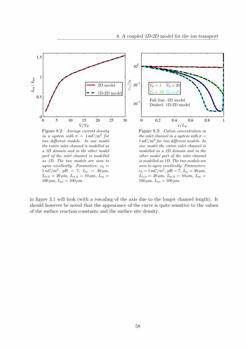
8. A coupled 1D-2D model for the ion transport

Figure 8.2: Average current densityin a system with σ = 1 mC/m2 fortwo different models. In one modelthe entire inlet channel is modelled asa 2D domain and in the other modelpart of the inlet channel is modelledas 1D. The two models are seen toagree excellently. Parameters: c0 =1 mC/m2, pH = 7, Lic = 30µm,Lir,0 = 20µm, Ltr,0 = 10µm, Lm =100µm, Loc = 100µm.

Figure 8.3: Cation concentration inthe inlet channel in a system with σ =1 mC/m2 for two different models. Inone model the entire inlet channel ismodelled as a 2D domain and in theother model part of the inlet channelis modelled as 1D. The two models areseen to agree excellently. Parameters:c0 = 1 mC/m2, pH = 7, Lic = 30µm,Lir,0 = 20µm, Ltr,0 = 10µm, Lm =100µm, Loc = 100µm.

in figure 3.1 will look (with a rescaling of the axis due to the longer channel length). Itshould however be noted that the appearance of the curve is quite sensitive to the valuesof the surface reaction constants and the surface site density.

58

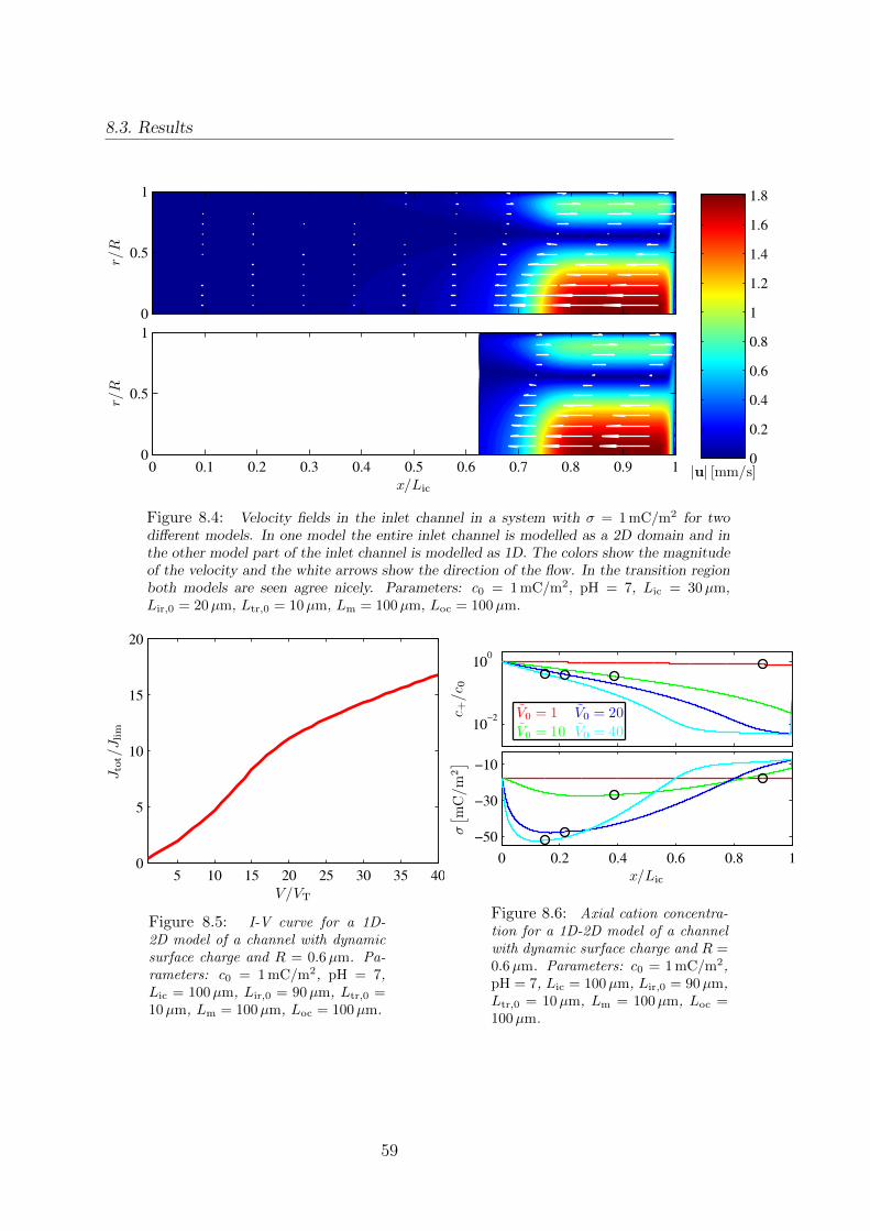
8.3. Results

Figure 8.4: Velocity fields in the inlet channel in a system with σ = 1 mC/m2 for twodifferent models. In one model the entire inlet channel is modelled as a 2D domain and inthe other model part of the inlet channel is modelled as 1D. The colors show the magnitudeof the velocity and the white arrows show the direction of the flow. In the transition regionboth models are seen agree nicely. Parameters: c0 = 1 mC/m2, pH = 7, Lic = 30µm,Lir,0 = 20µm, Ltr,0 = 10µm, Lm = 100µm, Loc = 100µm.

Figure 8.5: I-V curve for a 1D-2D model of a channel with dynamicsurface charge and R = 0.6µm. Pa-rameters: c0 = 1 mC/m2, pH = 7,Lic = 100µm, Lir,0 = 90µm, Ltr,0 =10µm, Lm = 100µm, Loc = 100µm.

Figure 8.6: Axial cation concentra-tion for a 1D-2D model of a channelwith dynamic surface charge and R =0.6µm. Parameters: c0 = 1 mC/m2,pH = 7, Lic = 100µm, Lir,0 = 90µm,Ltr,0 = 10µm, Lm = 100µm, Loc =100µm.

59

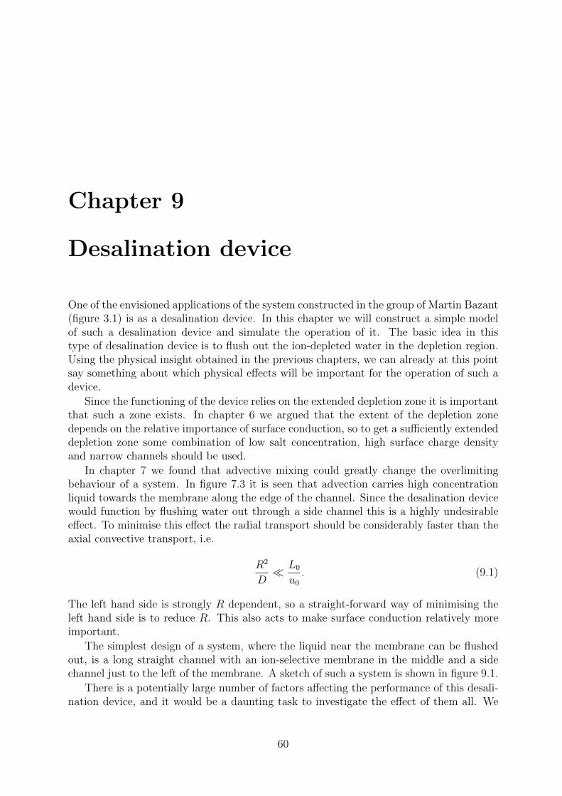
Chapter 9

Desalination device

One of the envisioned applications of the system constructed in the group of Martin Bazant(figure 3.1) is as a desalination device. In this chapter we will construct a simple modelof such a desalination device and simulate the operation of it. The basic idea in thistype of desalination device is to flush out the ion-depleted water in the depletion region.Using the physical insight obtained in the previous chapters, we can already at this pointsay something about which physical effects will be important for the operation of such adevice.

Since the functioning of the device relies on the extended depletion zone it is importantthat such a zone exists. In chapter 6 we argued that the extent of the depletion zonedepends on the relative importance of surface conduction, so to get a sufficiently extendeddepletion zone some combination of low salt concentration, high surface charge densityand narrow channels should be used.

In chapter 7 we found that advective mixing could greatly change the overlimitingbehaviour of a system. In figure 7.3 it is seen that advection carries high concentrationliquid towards the membrane along the edge of the channel. Since the desalination devicewould function by flushing water out through a side channel this is a highly undesirableeffect. To minimise this effect the radial transport should be considerably faster than theaxial convective transport, i.e.

R2

D L0

u0

. (9.1)

The left hand side is strongly R dependent, so a straight-forward way of minimising theleft hand side is to reduce R. This also acts to make surface conduction relatively moreimportant.

The simplest design of a system, where the liquid near the membrane can be flushedout, is a long straight channel with an ion-selective membrane in the middle and a sidechannel just to the left of the membrane. A sketch of such a system is shown in figure 9.1.

There is a potentially large number of factors affecting the performance of this desali-nation device, and it would be a daunting task to investigate the effect of them all. We

60

9.1. Implementation

Figure 9.1: Model of a desalination device.

therefore fix the radius at R = 0.6µm and the lengths at Lic = 20µm, Lm = 100µm,Loc = 100µm, Lout = R and Hout = R.

To transport liquid out of the system a net flow rate is needed. It is however clearthat the higher the flow from inlet reservoir to the side channel, the more salt will betransported towards the membrane. This will decrease the amount of depletion and thusincrease the concentration of the liquid being flushed out. A compromise therefore has tobe found between the need for a low concentration in the flushed out liquid and a highflow rate.

Initially, we do however only want to investigate if the flushed out liquid can getsufficiently desalinated. As the depletion is maximised for zero flow rate we will limitourselves to an investigation of that case as a start.

9.1 Implementation

In the left channel we implement boundary conditions and governing equations as done inchapter 7. Also, the mesh is constructed in roughly the same way. The corners where theinlet channel and side channel connects are rounded to avoid spurious edge effects. Againwe model the membrane region and the right channel using the 1D model.

At the side channel outlet we require the normal derivatives of the concentrationfields and the potential to vanish, implying purely convective transport of the salt ions.The tangential component of the velocity field and the normal derivative of the normalcomponent are both set to zero at the outlet.

The net flow rate in the system is controlled by electroosmosis and the pressure differ-ence between inlet reservoir and side channel. It is inconvenient to control the flow usingelectroosmosis as it is a function of the other system parameters c±, σ and φ. The pressuredifference is however easy to control independently of the other system parameters. Tomake sure that the pressure difference always has the value which will make the net flowrate zero we let it be a dependent variable and introduce an extra equation in the problem.

61

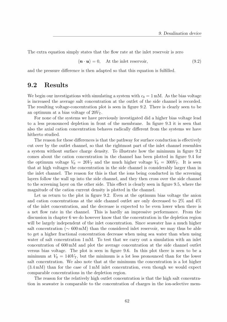
9. Desalination device

The extra equation simply states that the flow rate at the inlet reservoir is zero

〈n · u〉 = 0, At the inlet reservoir, (9.2)

and the pressure difference is then adapted so that this equation is fulfilled.

9.2 Results

We begin our investigations with simulating a system with c0 = 1 mM. As the bias voltageis increased the average salt concentration at the outlet of the side channel is recorded.The resulting voltage-concentration plot is seen in figure 9.2. There is clearly seen to bean optimum at a bias voltage of 20VT.

For none of the systems we have previously investigated did a higher bias voltage leadto a less pronounced depletion in front of the membrane. In figure 9.3 it is seen thatalso the axial cation concentration behaves radically different from the systems we havehitherto studied.

The reason for these differences is that the pathway for surface conduction is effectivelycut over by the outlet channel, so that the rightmost part of the inlet channel resemblesa system without surface charge density. To illustrate how the minimum in figure 9.2comes about the cation concentration in the channel has been plotted in figure 9.4 forthe optimum voltage V0 = 20VT and the much higher voltage V0 = 300VT. It is seenthat at high voltages the concentration in the side channel is considerably larger than inthe inlet channel. The reason for this is that the ions being conducted in the screeninglayers follow the wall up into the side channel, and they then cross over the side channelto the screening layer on the other side. This effect is clearly seen in figure 9.5, where themagnitude of the cation current density is plotted in the channel.

Let us return to the plot in figure 9.2. Even at the optimum bias voltage the anionand cation concentrations at the side channel outlet are only decreased to 2% and 4%of the inlet concentration, and the decrease is expected to be even lower when there isa net flow rate in the channel. This is hardly an impressive performance. From thediscussion in chapter 6 we do however know that the concentration in the depletion regionwill be largely independent of the inlet concentration. Since seawater has a much highersalt concentration (∼ 600 mM) than the considered inlet reservoir, we may thus be ableto get a higher fractional concentration decrease when using sea water than when usingwater of salt concentration 1 mM. To test that we carry out a simulation with an inletconcentration of 600 mM and plot the average concentration at the side channel outletversus bias voltage. The plot is seen in figure 9.6. In this plot there is seen to be aminimum at V0 = 140VT, but the minimum is a lot less pronounced than for the lowersalt concentration. We also note that at the minimum the concentration is a lot higher(3.4 mM) than for the case of 1 mM inlet concentration, even though we would expectcomparable concentrations in the depletion region.

The reason for the relatively high outlet concentration is that the high salt concentra-tion in seawater is comparable to the concentration of charges in the ion-selective mem-

62

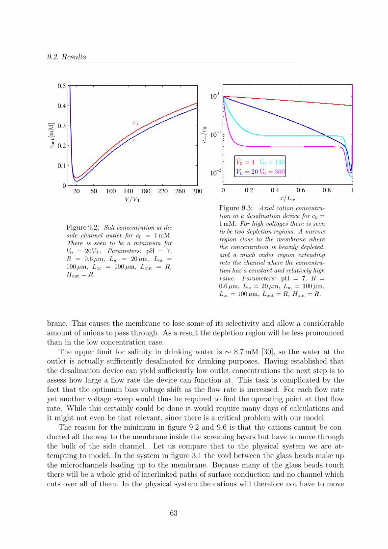
9.2. Results

Figure 9.2: Salt concentration at theside channel outlet for c0 = 1 mM.There is seen to be a minimum forV0 = 20VT. Parameters: pH = 7,R = 0.6µm, Lic = 20µm, Lm =100µm, Loc = 100µm, Lout = R,Hout = R.

Figure 9.3: Axial cation concentra-tion in a desalination device for c0 =1 mM. For high voltages there is seento be two depletion regions. A narrowregion close to the membrane wherethe concentration is heavily depleted,and a much wider region extendinginto the channel where the concentra-tion has a constant and relatively highvalue. Parameters: pH = 7, R =0.6µm, Lic = 20µm, Lm = 100µm,Loc = 100µm, Lout = R, Hout = R.

brane. This causes the membrane to lose some of its selectivity and allow a considerableamount of anions to pass through. As a result the depletion region will be less pronouncedthan in the low concentration case.

The upper limit for salinity in drinking water is ∼ 8.7 mM [30], so the water at theoutlet is actually sufficiently desalinated for drinking purposes. Having established thatthe desalination device can yield sufficiently low outlet concentrations the next step is toassess how large a flow rate the device can function at. This task is complicated by thefact that the optimum bias voltage shift as the flow rate is increased. For each flow rateyet another voltage sweep would thus be required to find the operating point at that flowrate. While this certainly could be done it would require many days of calculations andit might not even be that relevant, since there is a critical problem with our model.

The reason for the minimum in figure 9.2 and 9.6 is that the cations cannot be con-ducted all the way to the membrane inside the screening layers but have to move throughthe bulk of the side channel. Let us compare that to the physical system we are at-tempting to model. In the system in figure 3.1 the void between the glass beads make upthe microchannels leading up to the membrane. Because many of the glass beads touchthere will be a whole grid of interlinked paths of surface conduction and no channel whichcuts over all of them. In the physical system the cations will therefore not have to move

63

9. Desalination device

Figure 9.4: Cation concentration in a desalination device for c0 = 1 mM and two biasvoltages. Top: The cation concentration for the optimal bias voltage V0 = 20VT. Bottom:The cation concentration for a bias voltage of V0 = 300VT. The concentration in the sidechannel is seen to be considerably larger than in the inlet channel. Parameters: pH = 7,R = 0.6µm, Lic = 20µm, Lm = 100µm, Loc = 100µm, Lout = R, Hout = R.

Figure 9.5: Magnitude of the current density in a desalination device for c0 = 1 mM andV0 = 300VT. The majority of the current is carried in the screening layers and in the sidechannel. Parameters: pH = 7, R = 0.6µm, Lic = 20µm, Lm = 100µm, Loc = 100µm,Lout = R, Hout = R.

through the side channels, because there will be plenty of surface conduction paths theycan take. The minimum in figure 9.6 can thus be said to be an artifact of the modelling,and the physical system is expected to behave radically different from our model system.

Unfortunately there is no easy way to improve the modelling of the problem, since theexistence of the alternate surface conduction paths is linked to the geometry. To includethese paths we would have to make a full non-symmetric 3D model which would be ex-tremely computationally demanding.

Given that our model system was able to desalinate water sufficiently, even though thelack of surface conduction paths should make it less efficient than the physical system,

64

9.2. Results

Figure 9.6: Salt concentration at the side channel outlet for c0 = 600 mM (the cationand anion concentration curves overlap). There is seen to be a minimum for V0 = 140VT.Parameters: pH = 7, R = 0.6µm, Lic = 20µm, Lm = 100µm, Loc = 100µm, Lout = R,Hout = R.

the system in figure 3.1 could be a viable design for a desalination device. As we cannotproperly model the system, we can however neither predict the output of the system orat which efficiency it will run.

The considerations about the importance of different physical effects given in the startof the chapter are still expected to be valid.

65

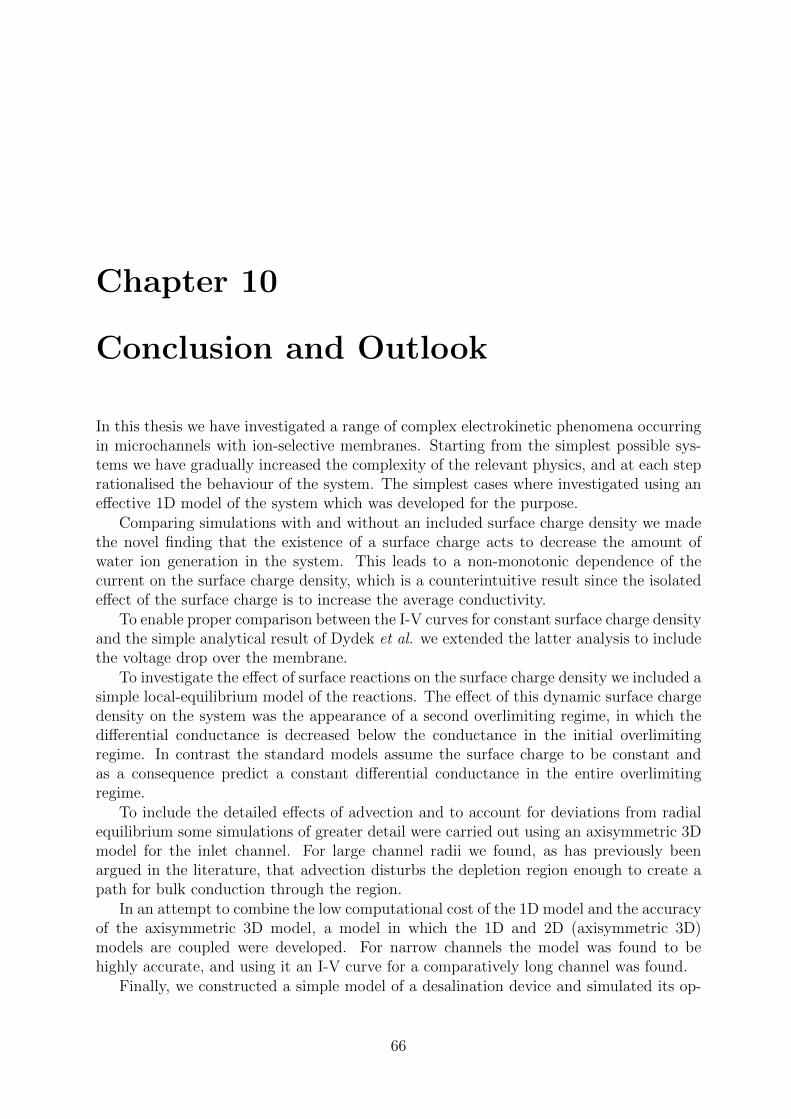
Chapter 10

Conclusion and Outlook

In this thesis we have investigated a range of complex electrokinetic phenomena occurringin microchannels with ion-selective membranes. Starting from the simplest possible sys-tems we have gradually increased the complexity of the relevant physics, and at each steprationalised the behaviour of the system. The simplest cases where investigated using aneffective 1D model of the system which was developed for the purpose.

Comparing simulations with and without an included surface charge density we madethe novel finding that the existence of a surface charge acts to decrease the amount ofwater ion generation in the system. This leads to a non-monotonic dependence of thecurrent on the surface charge density, which is a counterintuitive result since the isolatedeffect of the surface charge is to increase the average conductivity.

To enable proper comparison between the I-V curves for constant surface charge densityand the simple analytical result of Dydek et al. we extended the latter analysis to includethe voltage drop over the membrane.

To investigate the effect of surface reactions on the surface charge density we included asimple local-equilibrium model of the reactions. The effect of this dynamic surface chargedensity on the system was the appearance of a second overlimiting regime, in which thedifferential conductance is decreased below the conductance in the initial overlimitingregime. In contrast the standard models assume the surface charge to be constant andas a consequence predict a constant differential conductance in the entire overlimitingregime.

To include the detailed effects of advection and to account for deviations from radialequilibrium some simulations of greater detail were carried out using an axisymmetric 3Dmodel for the inlet channel. For large channel radii we found, as has previously beenargued in the literature, that advection disturbs the depletion region enough to create apath for bulk conduction through the region.

In an attempt to combine the low computational cost of the 1D model and the accuracyof the axisymmetric 3D model, a model in which the 1D and 2D (axisymmetric 3D)models are coupled were developed. For narrow channels the model was found to behighly accurate, and using it an I-V curve for a comparatively long channel was found.

Finally, we constructed a simple model of a desalination device and simulated its op-

66

eration. Although some interesting findings were made it was ultimately deemed futile tocontinue the simulations as the model had some fundamental shortcomings. The physicalrealisation of the system we were trying to model has a complicated asymmetric struc-ture, and in the course of our simulations we found this asymmetry, which we could notreplicate in our axisymmetric model, to be of critical importance.

The results of this thesis point out several directions which could be pursued in futurework.

Experimental verifications of the numerical results are of obvious interest. To enabledirect comparison between experiments and numerical simulations a number of steps wouldbe required. Firstly, a verification of the parameters in the dynamic surface charge modelwould be needed. This could be done by titration of a system including a frit of glassbeads. Because the reservoir boundary conditions are difficult to realise for small systemsthe numerical model would also have to be extended to include dynamics at the electrodes.

Another interesting study would be to extend the numerical models to allow for mod-elling of the asymmetric desalination device. A full 3D model resolving the screening layersis probably too computationally demanding, but it is likely that a simplified model, inwhich the screening layers and the bulk are treated as separate regions which only couplethrough an effective boundary condition, could yield reasonable results.

67

Bibliography

[1] B. Albert, D. Bray, K. Hopkin, A. Johnson, J. Lewis, M. Raff, K. Roberts, andP. Walter, Essential Cell Biology. Garland Science, 2004.

[2] H. Bruus, Theoretical Microfluidics. Oxford University Press, 2008.

[3] M. Bazant and T. Squires, “Induced-charge electrokinetic phenomena: Theory andmicrofluidic applications,” Physical Review Letters, vol. 92, pp. –, Feb. 2004.

[4] M. Bazant, M. Kilic, B. Storey, and A. Ajdari, “Towards an understanding of induced-charge electrokinetics at large applied voltages in concentrated solutions,” Advancesin colloid and interface science, vol. 152, no. 1-2, pp. 48–88, 2009.

[5] V. Nikonenko, N. Pismenskaya, E. Belova, P. Sistat, P. Huguet, G. Pourcelly, andC. Larchet, “Intensive current transfer in membrane systems: Modelling, mechanismsand application in electrodialysis,” Advances in colloid and interface science, vol. 160,no. 1-2, pp. 101–123, 2010.

[6] W. H. Smyrl and J. Newman, “Double layer structure at the limiting current,” Trans-actions of the Faraday Society, vol. 63, pp. 207–207, 1967.

[7] Y. I. Kharkats, “Theory of the exaltation effect and the effect of correlation exal-tation of migration current,” Journal of Electroanalytical Chemistry and InterfacialElectrochemistry, vol. 105, no. 1, pp. 97–114, 1979.

[8] M. B. Andersen, M. van Soestbergen, A. Mani, H. Bruus, P. M. Biesheuvel, and M. Z.Bazant, “Current-induced membrane discharge,” Arxiv preprint arXiv:1202.6448,pp. –, 2012.

[9] E. Dydek, B. Zaltzman, I. Rubinstein, D. Deng, A. Mani, and M. Bazant, “Over-limiting current in a microchannel,” Physical Review Letters, vol. 107, pp. –, Sept.2011.

[10] S. H. Behrens and D. G. Grier, “The charge of glass and silica surfaces,” The Journalof Chemical Physics, vol. 115, no. 14, pp. 6716–6716, 2001.

69

BIBLIOGRAPHY

[11] I. Borukhov, D. Andelman, and H. Orland, “Steric effects in electrolytes: A modifiedPoisson-Boltzmann equation,” Physical review letters, vol. 79, no. 3, pp. 435–438,1997.

[12] M. Kilic, M. Bazant, and A. Ajdari, “Steric effects in the dynamics of electrolytesat large applied voltages. ii. modified Poisson-Nernst-Planck equations,” PhysicalReview E, vol. 75, pp. –, Feb. 2007.

[13] M. Kilic, M. Bazant, and A. Ajdari, “Steric effects in the dynamics of electrolytes atlarge applied voltages. i. double-layer charging,” Physical Review E, vol. 75, pp. –,Feb. 2007.

[14] C. E. Housecroft and E. C. Constable, Chemistry. Pearson Education Limited, 2006.

[15] A. G. Volkov, S. Paula, and D. W. Deamer, “Two mechanisms of permeation of smallneutral molecules and hydrated ions across phospholipid bilayers,” Bioelectrochem-istry and bioenergetics, vol. 42, no. 2, pp. 153–160, 1997.

[16] C. Heitner-Wirguin, “Recent advances in perfluorinated ionomer membranes: struc-ture, properties and applications,” Journal of Membrane Science, vol. 120, no. 1,pp. 1–33, 1996.

[17] K. A. Mauritz and R. B. Moore, “State of understanding of nafion,” Chemical Re-views, vol. 104, pp. 4535–4586, Oct. 2004.

[18] DuPont, DuPont Nafion PFSA Membranes, 2009.

[19] T. Xu, “Ion exchange membranes: State of their development and perspective,”Journal of membrane science, vol. 263, no. 1, pp. 1–29, 2005.

[20] A. Elattar, A. Elmidaoui, N. Pismenskaia, C. Gavach, and G. Pourcelly, “Comparisonof transport properties of monovalent anions through anion-exchange membranes,”Journal of membrane science, vol. 143, no. 1, pp. 249–261, 1998.

[21] J. S. Mackie and P. Meares, “The sorption of electrolytes by a cation-exchange resinmembrane,” Proceedings of the Royal Society of London, vol. 232, pp. 485–498, 1955.

[22] Z. Lu, G. Polizos, D. D. Macdonald, and E. Manias, “State of water in perfluoro-sulfonic ionomer (nafion 117) proton exchange membranes,” Journal of The Electro-chemical Society, vol. 155, no. 2, pp. B163–B163, 2008.

[23] T. Hiemstra, W. Van Riemsdijk, and G. Bolt, “Multisite proton adsorption modelingat the solid/solution interface of (hydr)oxides: A new approach: I. model descrip-tion and evaluation of intrinsic reaction constants,” Journal of Colloid and InterfaceScience, vol. 133, pp. 91–104, Nov. 1989.

[24] R. K. Iler, The Chemistry of Silica. Wiley, 1979.

70

BIBLIOGRAPHY

[25] P. W. Atkins, Physical Chemistry. Oxford University Press, 1994.

[26] L. H. Olesen, “Computational fluid dynamics in microfluidic systems,” Master’s the-sis, Technical University of Denmark, 2003.

[27] COMSOL AB, COMSOL Multiphysics Reference Guide, 2011. Version 4.2.

[28] S. Brenner and L. R. Scott, The Mathematical Theory of Finite Element Methods.Springer, 1994.

[29] G. B. Arfken and H. J. Weber, Mathematical Methods for Physicists. Elsevier Aca-demic Press, 2005.

[30] The Council of the European Union, “Council directive 98/83/ec: on the quality ofwater intended for human consumption.” Official Journal of the European Commu-nities, 1998.

71