flow in microporous silicon carbide: an experimental...
TRANSCRIPT

Master Thesis, s031734 and s032056
Flow in Microporous Silicon Carbide:
an Experimental and Numerical Study
Kristoffer Gjendal and Henrik Bank Madsen
Main supervisor: Henrik BruusDepartment of Micro- and Nanotechnology
Technical University of Denmark
Co-supervisor: Thomas Eilkær HansenCoMeTas A/S
1 December 2008

ii
Abstract
Flow through porous silicon carbide (SiC) is studied in order to get an understanding ofthe parameters influencing the flow. As porous SiC is used to fabricate membranes, adeeper understanding of the flow through porous SiC would assist in the design process ofmore efficient membranes as well as with improving existing membranes.
The flow in porous SiC is described by Darcy’s law which is demonstrated both ana-lytically and by means of thorough experiments on different SiC-samples, such as simpleplugs, monotubes and so-called 24-channel tubes with a complex geometry. Experimentsare conducted both with pure SiC-substrates and with substrates coated with differentthin membrane layers.
From experiments with monotubes a permeability of the SiC-substrate is found andused in two numerical models developed to describe the flow in porous SiC. Resultsfrom the numerical models are compared to experimental results, and good correlationis achieved between simulations and experiments. The numerical models are used to de-velop optimized geometries with focus on increasing the permeate flow rate delivered fromthe tubes. These new design proposals are compared to existing membrane geometriesused by CoMeTas, the membrane company we cooperate with during the work for thisthesis, and the results show that significant increases in the permeate flow rate are ob-tained by making relatively small and simple geometrical changes.

iv ABSTRACT

Resume
Flow gennem porøs siliciumkarbid (SiC) bliver i denne afhandling undersøgt for at opnaen større forstaelse af de influerende parametre. Da porøs SiC anvendes til fremstillingenaf membraner, vil en større forstaelse af strømningerne gennem materialet være nyttig narnye membraner skal fremstilles eller eksisterende skal forbedres.
Flowet gennem porøs SiC er beskrevet ved Darcy’s lov, hvilket eftervises bade an-alytisk og ved gennemgribende eksperimenter med forskellige SiC-emner, sasom simpleskiver, enkeltkanalsrør og 24-kanalsrør med en kompleks geometri. Eksperimenter udføresbade med rene SiC-substrater og med substrater, der er coatet med forskellige tynde mem-branlag.
Permeabiliteten i SiC-substratet findes ud fra eksperimenter med enkeltkanalsrør, ogden bliver anvendt i to udviklede numeriske modeller, som beskriver strømningerne i porøsSiC. Resultaterne fra de to numeriske modeller bliver sammenlignet med resultaterne fraeksperimenterne og god overensstemmelse findes mellem simuleringer og eksperimenter.De numeriske modeller bliver anvendt til at udvikle optimerede geometrier med fokus paat øge permeat flowet gennem rørene. Permeat flowet fra optimerede rør bliver sammen-lignet med permeat flowet fra standard membraner fra CoMeTas, som er det firma vi harsamarbejdet med i vores afgangsprojekt. Denne sammenligning viser at det er muligt atopna store forøgelser af permeat flowet ved relativt sma og simple indgreb.

vi RESUME
Preface
This thesis, titled ”Flow in Microporous Silicon Carbide: an Experimental and Numer-ical Study”, has been submitted in order to obtain the Master of Science degree at theTechnical University of Denmark (DTU). The project work was carried out within theTheoretical Microfluidics (TMF) group at the Department of Micro- and Nanotechnol-ogy (DTU Nanotech) and in cooperation with the membrane company CoMeTas duringthe period from February 2008 to December 2008, corresponding to a credit of 45 ECTSpoints.
First of all we want to thank our supervisor Henrik Bruus for invaluable guidanceand inspiration throughout the thesis work and for always having extra time to spareto discuss different issues. Further we are thankful to our co-supervisor Thomas EilkærHansen and the rest of the staff at CoMeTas for their help and encouragement especiallyduring the experimental part of the project. We also acknowledge CoMeTas for puttingthe experimental setup at our disposal and for giving us free hands during the entireproject. We have also appreciated the ideas and comments offered by the rest of the TMFgroup, especially at the weekly group meetings.
We are grateful to Johnny Marcher (technical director at LiqTech) for lending us equip-ment and for his good advise during the fabrication and geometrical optimization process.Furthermore we want to express our gratitude to Alexander Shapiro (associate professor,Department of Chemical and Biochemical Engineering, DTU) and Duc Thuong Vu (tech-nician, Department of Chemical and Biochemical Engineering, DTU) for introducing usto the CT-scanner and its possibilities. Also we thank Jesper Lybæk from the companyJaka Metal for water-jet cutting our plugs.
Finally, we want to thank all those not mentioned above, but who have offered theirassistance or helped us in one way or another during our project.
Kristoffer Gjendal and Henrik Bank MadsenDepartment of Micro- and Nanotechnology
Technical University of Denmark1 December 2008

viii PREFACE

Contents
List of figures xv
List of tables xvii
List of symbols xix
1 Introduction 11.1 Membrane filtration . . . . . . . . . . . . . . . . . . . . . . . . . . . . . . . 11.2 Membranes and silicon carbide . . . . . . . . . . . . . . . . . . . . . . . . . 21.3 Objective and motivation . . . . . . . . . . . . . . . . . . . . . . . . . . . . 21.4 Outline . . . . . . . . . . . . . . . . . . . . . . . . . . . . . . . . . . . . . . 3
2 Basic theory and considerations 52.1 Fundamental equations . . . . . . . . . . . . . . . . . . . . . . . . . . . . . . 52.2 Flow in porous media . . . . . . . . . . . . . . . . . . . . . . . . . . . . . . 6
2.2.1 Permeability . . . . . . . . . . . . . . . . . . . . . . . . . . . . . . . 62.2.2 Flow regions and Darcy’s law . . . . . . . . . . . . . . . . . . . . . . 72.2.3 1D flow through porous plug in a pipe . . . . . . . . . . . . . . . . . 82.2.4 2D flow in pipe with porous walls . . . . . . . . . . . . . . . . . . . . 10
2.3 General channel flow . . . . . . . . . . . . . . . . . . . . . . . . . . . . . . . 112.4 Equivalent circuit model . . . . . . . . . . . . . . . . . . . . . . . . . . . . . 132.5 The Laplace equation in 1D and 2D Darcy flow . . . . . . . . . . . . . . . . 13
3 Fabrication and characterization of SiC-samples 153.1 Fabrication of SiC-plugs and tubes . . . . . . . . . . . . . . . . . . . . . . . 15
3.1.1 Plugs . . . . . . . . . . . . . . . . . . . . . . . . . . . . . . . . . . . 153.1.2 Monotubes . . . . . . . . . . . . . . . . . . . . . . . . . . . . . . . . 163.1.3 24-channel tubes . . . . . . . . . . . . . . . . . . . . . . . . . . . . . 213.1.4 Coating . . . . . . . . . . . . . . . . . . . . . . . . . . . . . . . . . . 22
3.2 Characterization methods . . . . . . . . . . . . . . . . . . . . . . . . . . . . 233.2.1 CT-scan . . . . . . . . . . . . . . . . . . . . . . . . . . . . . . . . . . 233.2.2 Porosity . . . . . . . . . . . . . . . . . . . . . . . . . . . . . . . . . . 243.2.3 Capillary rise . . . . . . . . . . . . . . . . . . . . . . . . . . . . . . . 243.2.4 Bubble point . . . . . . . . . . . . . . . . . . . . . . . . . . . . . . . 24
x CONTENTS
4 Experimental setup 254.1 Description of the experimental setup . . . . . . . . . . . . . . . . . . . . . 25
4.1.1 Setup for plug experiments . . . . . . . . . . . . . . . . . . . . . . . 284.1.2 Setup for tube experiments . . . . . . . . . . . . . . . . . . . . . . . 29
4.2 Improvements of the experimental setup . . . . . . . . . . . . . . . . . . . . 30
5 Experiments with SiC-substrates 335.1 Plugs . . . . . . . . . . . . . . . . . . . . . . . . . . . . . . . . . . . . . . . . 33
5.1.1 Errors on the measured data . . . . . . . . . . . . . . . . . . . . . . 355.1.2 Challenges . . . . . . . . . . . . . . . . . . . . . . . . . . . . . . . . 365.1.3 Results . . . . . . . . . . . . . . . . . . . . . . . . . . . . . . . . . . 38
5.2 Monotubes . . . . . . . . . . . . . . . . . . . . . . . . . . . . . . . . . . . . 415.2.1 Short thin-walled monotubes . . . . . . . . . . . . . . . . . . . . . . 435.2.2 Thick-walled monotubes . . . . . . . . . . . . . . . . . . . . . . . . . 455.2.3 Long thin-walled monotubes . . . . . . . . . . . . . . . . . . . . . . 475.2.4 Re-sintered monotubes . . . . . . . . . . . . . . . . . . . . . . . . . . 47
5.3 24-channel tubes . . . . . . . . . . . . . . . . . . . . . . . . . . . . . . . . . 485.4 Summary . . . . . . . . . . . . . . . . . . . . . . . . . . . . . . . . . . . . . 50
6 Experiments with coated SiC-tubes 536.1 Thin-walled monotubes . . . . . . . . . . . . . . . . . . . . . . . . . . . . . 53
6.1.1 0.1 µm membrane . . . . . . . . . . . . . . . . . . . . . . . . . . . . 546.1.2 0.04 µm membrane . . . . . . . . . . . . . . . . . . . . . . . . . . . . 556.1.3 Investigation of the membrane thickness . . . . . . . . . . . . . . . . 566.1.4 Comparison of substrate and membranes . . . . . . . . . . . . . . . 58
6.2 24-channel tubes . . . . . . . . . . . . . . . . . . . . . . . . . . . . . . . . . 596.2.1 0.1 µm membrane . . . . . . . . . . . . . . . . . . . . . . . . . . . . 596.2.2 0.04 µm membrane . . . . . . . . . . . . . . . . . . . . . . . . . . . . 606.2.3 Investigation of the membrane thickness . . . . . . . . . . . . . . . . 616.2.4 Comparison of substrate and membranes . . . . . . . . . . . . . . . 63
6.3 Summary . . . . . . . . . . . . . . . . . . . . . . . . . . . . . . . . . . . . . 64
7 Numerical models and flow simulations 677.1 Comsol model . . . . . . . . . . . . . . . . . . . . . . . . . . . . . . . . . . 67
7.1.1 24-channel tube . . . . . . . . . . . . . . . . . . . . . . . . . . . . . . 687.2 Equivalent circuit model . . . . . . . . . . . . . . . . . . . . . . . . . . . . . 70
7.2.1 Monotube . . . . . . . . . . . . . . . . . . . . . . . . . . . . . . . . . 707.2.2 24-channel tube . . . . . . . . . . . . . . . . . . . . . . . . . . . . . . 73
7.3 Membrane simulations . . . . . . . . . . . . . . . . . . . . . . . . . . . . . . 787.3.1 Comsol model . . . . . . . . . . . . . . . . . . . . . . . . . . . . . . 787.3.2 Equivalent circuit model . . . . . . . . . . . . . . . . . . . . . . . . . 80
7.4 Summary . . . . . . . . . . . . . . . . . . . . . . . . . . . . . . . . . . . . . 81
CONTENTS xi
8 Geometrical optimization 838.1 Optimizing surface area . . . . . . . . . . . . . . . . . . . . . . . . . . . . . 838.2 Optimizing channel dimensions . . . . . . . . . . . . . . . . . . . . . . . . . 868.3 Proposal for a new design . . . . . . . . . . . . . . . . . . . . . . . . . . . . 898.4 Improvements and comparison of large tubes . . . . . . . . . . . . . . . . . 90
8.4.1 Parallel connected tubes . . . . . . . . . . . . . . . . . . . . . . . . . 918.4.2 New design of a COM-144-865-(2*2)-0.04 . . . . . . . . . . . . . . . 92
8.5 Summary . . . . . . . . . . . . . . . . . . . . . . . . . . . . . . . . . . . . . 95
9 Conclusion and outlook 979.1 Conclusion . . . . . . . . . . . . . . . . . . . . . . . . . . . . . . . . . . . . 979.2 Outlook . . . . . . . . . . . . . . . . . . . . . . . . . . . . . . . . . . . . . . 98
A Characterization methods 101A.1 Porosity . . . . . . . . . . . . . . . . . . . . . . . . . . . . . . . . . . . . . . 101A.2 Capillary rise . . . . . . . . . . . . . . . . . . . . . . . . . . . . . . . . . . . 102A.3 Bubble point . . . . . . . . . . . . . . . . . . . . . . . . . . . . . . . . . . . 103
B Investigation of the experimental setup 107B.1 Pressure drop from PT01 to housing . . . . . . . . . . . . . . . . . . . . . . 108B.2 Pressure drop from housing to PT02 . . . . . . . . . . . . . . . . . . . . . . 108B.3 Pressure drop from housing to PT03 . . . . . . . . . . . . . . . . . . . . . . 109B.4 Larger tubes from PT01 and PT03 to the housing . . . . . . . . . . . . . . 110
C Additional experiments 111C.1 Cross-flow experiments . . . . . . . . . . . . . . . . . . . . . . . . . . . . . . 111
C.1.1 Monotubes . . . . . . . . . . . . . . . . . . . . . . . . . . . . . . . . 111C.1.2 24-channel tubes . . . . . . . . . . . . . . . . . . . . . . . . . . . . . 112
C.2 Long thin-walled monotube . . . . . . . . . . . . . . . . . . . . . . . . . . . 113C.3 Experiments with 1 µm membrane . . . . . . . . . . . . . . . . . . . . . . . 114
C.3.1 Monotubes . . . . . . . . . . . . . . . . . . . . . . . . . . . . . . . . 114C.3.2 24-channel tubes . . . . . . . . . . . . . . . . . . . . . . . . . . . . . 114
D Module of hexagonal tubes 117
E Data sheet 119
F Working drawings 121F.1 Part for extruder head . . . . . . . . . . . . . . . . . . . . . . . . . . . . . . 122F.2 Thin inner cylinder . . . . . . . . . . . . . . . . . . . . . . . . . . . . . . . . 123F.3 Thick inner cylinder . . . . . . . . . . . . . . . . . . . . . . . . . . . . . . . 124
Bibliography 125

xii CONTENTS
List of Figures
1.1 Principle of dead-end and cross-flow filtration . . . . . . . . . . . . . . . . . 1
2.1 Flow regimes in a porous media . . . . . . . . . . . . . . . . . . . . . . . . . 72.2 Pipe with a porous plug . . . . . . . . . . . . . . . . . . . . . . . . . . . . . 92.3 Pipe with porous walls . . . . . . . . . . . . . . . . . . . . . . . . . . . . . . 102.4 Simple plug and tube geometry . . . . . . . . . . . . . . . . . . . . . . . . . 14
3.1 Plug plate . . . . . . . . . . . . . . . . . . . . . . . . . . . . . . . . . . . . . 163.2 Extruder setup . . . . . . . . . . . . . . . . . . . . . . . . . . . . . . . . . . 173.3 Pictures of extruder head . . . . . . . . . . . . . . . . . . . . . . . . . . . . 183.4 Pictures of monotubes . . . . . . . . . . . . . . . . . . . . . . . . . . . . . . 193.5 Drying table . . . . . . . . . . . . . . . . . . . . . . . . . . . . . . . . . . . . 203.6 24-channel tube . . . . . . . . . . . . . . . . . . . . . . . . . . . . . . . . . . 223.7 CT-pictures of a monotube . . . . . . . . . . . . . . . . . . . . . . . . . . . 23
4.1 Diagram of experimental setup . . . . . . . . . . . . . . . . . . . . . . . . . 264.2 Pictures of experimental setup . . . . . . . . . . . . . . . . . . . . . . . . . 274.3 Plug mounted in housing . . . . . . . . . . . . . . . . . . . . . . . . . . . . 284.4 Tube mounted in housing . . . . . . . . . . . . . . . . . . . . . . . . . . . . 294.5 New parts for the experimental setup . . . . . . . . . . . . . . . . . . . . . . 31
5.1 Pictures of the plugs . . . . . . . . . . . . . . . . . . . . . . . . . . . . . . . 345.2 Pressure measurement . . . . . . . . . . . . . . . . . . . . . . . . . . . . . . 355.3 Contaminated plug measurements . . . . . . . . . . . . . . . . . . . . . . . 365.4 Linear plug measurement . . . . . . . . . . . . . . . . . . . . . . . . . . . . 395.5 Plug measurements . . . . . . . . . . . . . . . . . . . . . . . . . . . . . . . . 405.6 Permeability of the plugs . . . . . . . . . . . . . . . . . . . . . . . . . . . . 415.7 Flow rate dependence on water temperature . . . . . . . . . . . . . . . . . . 425.8 Linear monotube measurement . . . . . . . . . . . . . . . . . . . . . . . . . 445.9 Thin-walled monotube measurements . . . . . . . . . . . . . . . . . . . . . . 455.10 Thick-walled monotube measurements . . . . . . . . . . . . . . . . . . . . . 465.11 Cracked thick-walled monotube . . . . . . . . . . . . . . . . . . . . . . . . . 465.12 Re-sintering of monotube . . . . . . . . . . . . . . . . . . . . . . . . . . . . 475.13 Nonlinear 24-channel tube measurement . . . . . . . . . . . . . . . . . . . . 48
xiv LIST OF FIGURES
5.14 24-channel tube measurements . . . . . . . . . . . . . . . . . . . . . . . . . 50
6.1 Thin-walled monotubes coated with 0.1µm membrane . . . . . . . . . . . . 546.2 Thin-walled monotubes coated with 0.04µm membrane . . . . . . . . . . . 566.3 Pictures of membranes, thin-walled monotubes . . . . . . . . . . . . . . . . 576.4 Comparison of thin-walled monotubes . . . . . . . . . . . . . . . . . . . . . 596.5 24-channel tubes coated with 0.1µm membrane . . . . . . . . . . . . . . . . 606.6 24-channel tubes coated with 0.04µm membrane . . . . . . . . . . . . . . . 616.7 Pictures of 0.1µm membrane, 24-channel tubes . . . . . . . . . . . . . . . . 626.8 Pictures of 0.04 µm membrane, 24-channel tubes . . . . . . . . . . . . . . . 636.9 Comparison of 24-channel tubes . . . . . . . . . . . . . . . . . . . . . . . . . 64
7.1 Geometry of 24-channel tube . . . . . . . . . . . . . . . . . . . . . . . . . . 687.2 Convergence of the permeate flow rate, 24-channel tube . . . . . . . . . . . 697.3 Pressure distribution, 24-channel tube . . . . . . . . . . . . . . . . . . . . . 697.4 EC model of a monotube . . . . . . . . . . . . . . . . . . . . . . . . . . . . 717.5 Comparison of the measurements and simulations of short thin-walled mono-
tube . . . . . . . . . . . . . . . . . . . . . . . . . . . . . . . . . . . . . . . . 727.6 Comparison of the measurements and simulations of long thin-walled mono-
tube . . . . . . . . . . . . . . . . . . . . . . . . . . . . . . . . . . . . . . . . 727.7 EC model of 24-channel tube . . . . . . . . . . . . . . . . . . . . . . . . . . 737.8 Segment of the 3D EC model . . . . . . . . . . . . . . . . . . . . . . . . . . 747.9 3D EC model of 24-channel tube . . . . . . . . . . . . . . . . . . . . . . . . 757.10 Pressure and permeate flow rate along the length of a 24-channel tube . . . 767.11 Comparison of pressure drop from experiments and simulations along the
length of a 24-channel tube . . . . . . . . . . . . . . . . . . . . . . . . . . . 777.12 Comparison of the measurements and simulations for a 24-channel tube . . 787.13 Pressure solution in 24-channel tube with 0.04 µm membrane . . . . . . . . 797.14 Pressure and permeate flow a long the length of a 24-channel tube coated
with 0.04µm membrane . . . . . . . . . . . . . . . . . . . . . . . . . . . . . 807.15 Comparison of the measurements and simulations of 24-channel tube coated
with 0.04µm membrane . . . . . . . . . . . . . . . . . . . . . . . . . . . . . 81
8.1 2D Comsol pressure plot of 24-channel tube with a cut . . . . . . . . . . . 848.2 2D Comsol pressure plot of 24-channel tube with cut and quadrilateral hole 858.3 2D Comsol pressure plot of 21-channel tube with bigger channels . . . . . 868.4 Influence of channel size . . . . . . . . . . . . . . . . . . . . . . . . . . . . . 878.5 Influence of channel length . . . . . . . . . . . . . . . . . . . . . . . . . . . . 888.6 Comsol pressure plot of 18-channel tube with cut into center hole . . . . . 898.7 Comparison of the 18-channel tube and the 24-channel tube . . . . . . . . . 908.8 Module containing 19 original 24-channel tubes . . . . . . . . . . . . . . . . 918.9 Pressure distribution in the COM-144-865-(2*2)-0.04 . . . . . . . . . . . . . 938.10 Pressure plot of the COM-144-865-(2*2)-0.04 with several cuts . . . . . . . 938.11 Design suggestion of a large membrane . . . . . . . . . . . . . . . . . . . . . 94

LIST OF FIGURES xv
8.12 2D Comsol pressure distribution of new design suggestion . . . . . . . . . 94
9.1 Preliminary experiments with optimized structure . . . . . . . . . . . . . . 98
A.1 Capillary rise method . . . . . . . . . . . . . . . . . . . . . . . . . . . . . . 102A.2 Bubble point method . . . . . . . . . . . . . . . . . . . . . . . . . . . . . . . 104
C.1 Cross-flow measurements with monotube . . . . . . . . . . . . . . . . . . . . 112C.2 Cross-flow measurements with 24-channel tube . . . . . . . . . . . . . . . . 112C.3 Long thin-walled monotube . . . . . . . . . . . . . . . . . . . . . . . . . . . 113C.4 Measurements with monotubes coated with 1µm membrane . . . . . . . . . 115C.5 Measurements with 24-channel tubes coated with 1µm membrane . . . . . 115
D.1 Pressure distribution in a hexagonal tube . . . . . . . . . . . . . . . . . . . 117D.2 Module containing 37 hexagonal tubes . . . . . . . . . . . . . . . . . . . . . 118
F.1 Part for extruder head . . . . . . . . . . . . . . . . . . . . . . . . . . . . . . 122F.2 Thin inner cylinder . . . . . . . . . . . . . . . . . . . . . . . . . . . . . . . . 123F.3 Thick inner cylinder . . . . . . . . . . . . . . . . . . . . . . . . . . . . . . . 124

xvi LIST OF FIGURES
List of Tables
4.1 List of error for different pressure transmitters . . . . . . . . . . . . . . . . 31
5.1 Measured permeabilities of the SiC . . . . . . . . . . . . . . . . . . . . . . . 51
6.1 Measured membrane thicknesses on the tubes . . . . . . . . . . . . . . . . . 65
8.1 Comsol results from the original 24-channel tube . . . . . . . . . . . . . . 84
A.1 Results from capillary rise experiment . . . . . . . . . . . . . . . . . . . . . 103A.2 Results from bubble point experiment . . . . . . . . . . . . . . . . . . . . . 105
B.1 Pressure drop from PT01 to housing . . . . . . . . . . . . . . . . . . . . . . 108B.2 Pressure drop from housing to PT02 . . . . . . . . . . . . . . . . . . . . . . 109B.3 Pressure drop from housing to PT03 . . . . . . . . . . . . . . . . . . . . . . 109B.4 Pressure drop in tubes with different diameters (PT01 to housing). . . . . . 110B.5 Pressure drop in tubes with different diameters (housing to PT03) . . . . . 110

xviii LIST OF TABLES

List of symbols
Symbol Description UnitA Area m2
a Radius of a cylinder m, mmc0 Dimensionless shape factorD, d Diameter m, mm, µme Pipe roughness m, mmf Friction factorg Gravitational acceleration m s−2
g Gravitational acceleration vector m s−2
H, h Height m, mmhl Major head loss m2 s−2
hlm Minor head loss m2 s−2
hlT Total head loss m2 s−2
I Electric current AKl Loss coefficientk Permeability m2
L, ` Length m, mmL0 Characteristic length m, mmm Mass kgn Normal vectorp Pressure Pa, barp0 Atmospheric gauge pressure Pa, barp Time averaged mean gauge pressure Pa, barp∗ Reference pressure Pa, bar∆psurf Young-Laplace pressure drop Pa, barQ Volume flow rate m3 s−1, m3 h−1
R Electric resistance ΩRhyd Hydraulic resistance Pa s m−3
Rc Channel resistance Pa s2 m−6
Re Reynolds numberr Radius m, mmS Surface area pr. volume of particles m−1
T Time scale st Time st Normalized time

xx LIST OF SYMBOLS
Symbol Description Unit∆U Electric potential difference VV Volume m3
V Time averaged mean velocity m s−1
V0 Characteristic velocity m s−1
v Velocity vector m s−1
v Velocity m s−1
w Wall thickness m, mmwe Actual flow distance m, mmz Vertical position m
α Kinetic energy coefficientβ Dissipative force Pa s m−2
γ Surface tension J m−2, mJ m−2
ε Errorζ Correlation coefficientη Dynamic viscosity Pa sθ Polar angleκ Kozeny-Carman constantλ Constant mρ Mass density kg m−3
τ Tortuosityφ Porosity (volume fraction)
Subscript Descriptionb Bubble pointc Channeld Dryf Feedm Meann Normalo Outerp Permeater Retentates Substratetm Transmembranew Water

Chapter 1
Introduction
1.1 Membrane filtration
Flow through porous media is encountered in many different types of engineering, one ofthe most important being membrane filtration. Filtration is traditionally defined as theseparation of particulate material from a fluid by the passage of the fluid through a porousmaterial (the filter) that retains the particles on or within itself. The driving force in thisprocess is the pressure difference applied across the filter. Membrane filtration, on theother hand, has a broader definition. It includes not only the separation of particulatematter, but also the separation of soluble components. Furthermore, membrane filtrationdiffers from conventional filtration because material, which is unable to permeate throughthe membrane, may remain in suspension upstream of the membrane instead of beingretained on or within the filter. For further information about filtration see [5, 6].
Generally, two methods are used in membrane filtration. In the most simple andconventional method the fluid permeates through the membrane while the particulatematerial is rejected at the surface of the membrane, thus the filtered solids are allowed to
(a)
Permeate
Feed
Membrane
(b)
Feed
Permeate
Retentate
Membrane
Figure 1.1: (a) Principle of dead-end filtration. The fluid permeates through the porous membrane, whileparticles larger than the pore size in the membrane are rejected at the surface of the membrane and buildup as a filter cake. (b) Principle of cross-flow filtration. The direction of the feed stream is tangentiallyover the surface of the membrane in order to sweep the rejected particles away from the membrane. Thefluid is separated into two product streams, the permeate, which is depleted of the rejected particles, andthe retentate (or concentrate), which is enriched in those particles. This figure is made with inspirationfrom [6].

2 CHAPTER 1. INTRODUCTION
build up as a so-called filter cake on the surface of the membrane, see Fig. 1.1(a). Thismethod is referred to as dead-end filtration. It is a very energy efficient method, but itis rarely used because the permeation rate through the combined membrane and surfacecake layer would, in most applications, fall to very low levels. Therefore another method,the so-called cross-flow method, is widely used in membrane filtration, see Fig. 1.1(b).In this method the feed flow is tangential to the surface of the membrane in order tosweep rejected particles and solutes away. The feed fluid is separated into two productstreams, the permeate, which is depleted of the rejected particles, and the retentate (orconcentrate), which is enriched in those particles. The feed fluid is defined as the initialfluid mixture before the membrane. The permeate fluid is defined as the stream thatemerges from the membrane and is depleted of the rejected particulate material. Theretentate (or concentrate) is defined as the stream on the upstream side of the membrane,which is enriched in the same components [5, 6].
This thesis deals only with the pure water flow through a porous membrane, not witha fluid mixture containing particulate material. Therefore the filtration process itself willnot be investigated.
1.2 Membranes and silicon carbide
Copenhagen Membrane Technology A/S (CoMeTas) was founded in 2006 at Scion, DTU,and is today situated in Bagsværd. The company develops and manufactures ceramicmembranes of porous silicon carbide (SiC) for both dead-end and cross-flow applications.CoMeTas’ membranes are so-called asymmetric membranes, meaning that they consist oftwo different layers. The main structure, called the substrate or carrier, is made of largeSiC-particles sintered together, and this substrate supports one or more thin top layersconsisting of smaller SiC-particles, called the membrane layers. The membrane layers havea thickness of approximately 50µm to 200µm and a mean pore size of around 0.01µmto 0.5µm, while the substrate thickness is minimum 0.8mm and has a mean pore size of10µm to 20µm, [19, 20]. This design increases the flow rate through the filter, as theresistance in the substrate is significantly lower than the resistance in the membrane layerdue to the larger particles. The pore size in the membrane layer determines the size of theparticulate material that is rejected, and it can be changed by varying the SiC-particlecomposition in the membrane layer.
Silicon carbide membranes have many advantages. They are very wear resistant, asSiC is one of the hardest materials known, they have a relatively high flow rate comparedto other porous ceramic membranes, and they have high chemical and physical stabilityand thus a long service life-time. All these properties make porous SiC a very promisingmaterial with respect to membrane applications.
1.3 Objective and motivation
As CoMeTas is a newly started company, the knowledge concerning the flow in theirmembranes is still limited. Theoretical and experimental investigations of the flow in SiC-
1.4 Outline 3
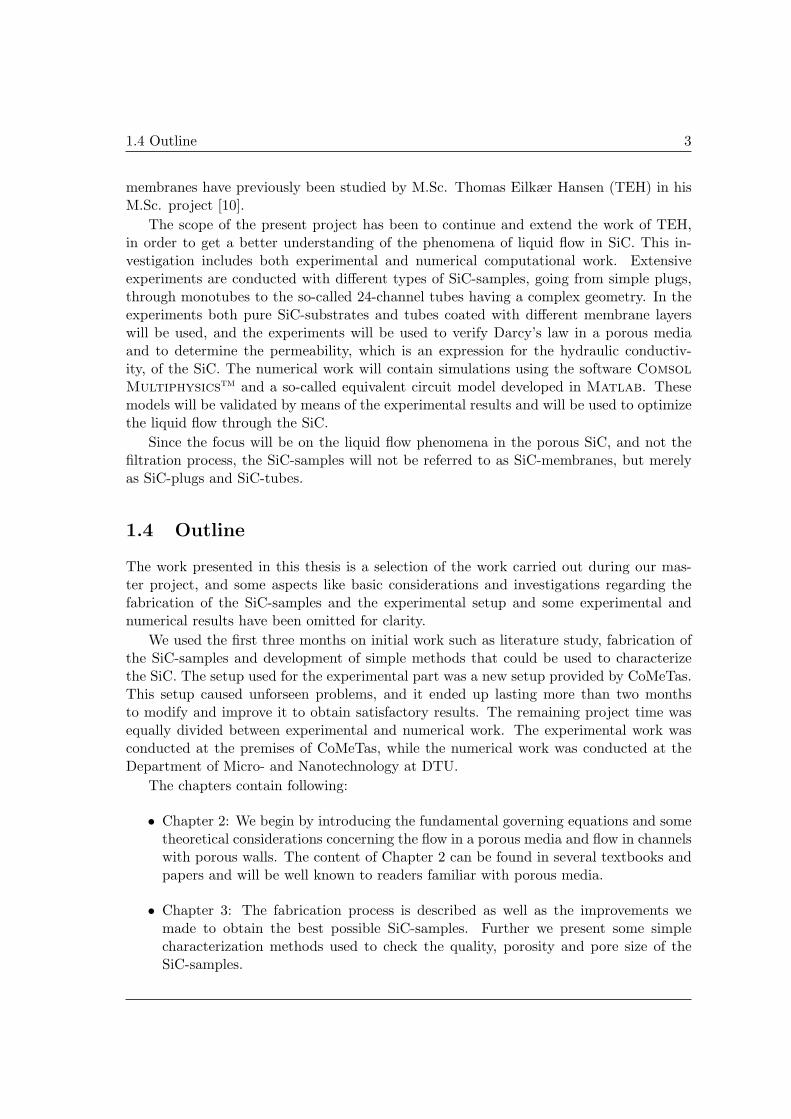
membranes have previously been studied by M.Sc. Thomas Eilkær Hansen (TEH) in hisM.Sc. project [10].
The scope of the present project has been to continue and extend the work of TEH,in order to get a better understanding of the phenomena of liquid flow in SiC. This in-vestigation includes both experimental and numerical computational work. Extensiveexperiments are conducted with different types of SiC-samples, going from simple plugs,through monotubes to the so-called 24-channel tubes having a complex geometry. In theexperiments both pure SiC-substrates and tubes coated with different membrane layerswill be used, and the experiments will be used to verify Darcy’s law in a porous mediaand to determine the permeability, which is an expression for the hydraulic conductiv-ity, of the SiC. The numerical work will contain simulations using the software ComsolMultiphysicstm and a so-called equivalent circuit model developed in Matlab. Thesemodels will be validated by means of the experimental results and will be used to optimizethe liquid flow through the SiC.
Since the focus will be on the liquid flow phenomena in the porous SiC, and not thefiltration process, the SiC-samples will not be referred to as SiC-membranes, but merelyas SiC-plugs and SiC-tubes.
1.4 Outline
The work presented in this thesis is a selection of the work carried out during our mas-ter project, and some aspects like basic considerations and investigations regarding thefabrication of the SiC-samples and the experimental setup and some experimental andnumerical results have been omitted for clarity.
We used the first three months on initial work such as literature study, fabrication ofthe SiC-samples and development of simple methods that could be used to characterizethe SiC. The setup used for the experimental part was a new setup provided by CoMeTas.This setup caused unforseen problems, and it ended up lasting more than two monthsto modify and improve it to obtain satisfactory results. The remaining project time wasequally divided between experimental and numerical work. The experimental work wasconducted at the premises of CoMeTas, while the numerical work was conducted at theDepartment of Micro- and Nanotechnology at DTU.
The chapters contain following:
• Chapter 2: We begin by introducing the fundamental governing equations and sometheoretical considerations concerning the flow in a porous media and flow in channelswith porous walls. The content of Chapter 2 can be found in several textbooks andpapers and will be well known to readers familiar with porous media.
• Chapter 3: The fabrication process is described as well as the improvements wemade to obtain the best possible SiC-samples. Further we present some simplecharacterization methods used to check the quality, porosity and pore size of theSiC-samples.

4 CHAPTER 1. INTRODUCTION
• Chapter 4: The experimental setup is shortly described along with the improvementswe made to obtain satisfactory results.
• Chapter 5: The experiments conducted with the substrate SiC-samples are presentedhere together with the obtained results. These experiments include plugs with fourdifferent thicknesses, monotubes with two different wall thicknesses and 24-channeltubes.
• Chapter 6: This chapter describes the experiments carried out on monotubes and24-channel tubes coated with membrane layers in the same manner as CoMeTas’membranes. The obtained results are presented together with a short investigationof the quality and thickness of the membrane layers.
• Chapter 7: Two numerical models are developed, a simple 2D model made in Com-sol on the basis of potential flow and the Laplace equation, and a 3D equivalentcircuit model made in Matlab. Results obtained with the two models are presentedand compared with experimental results.
• Chapter 8: Using the developed numerical models, new membrane designs are pre-sented with the focus on increasing the permeating water flow. The performance ofthe proposed designs are compared with existing membranes from CoMeTas.
• Chapter 9: The thesis is rounded off with a conclusion and an outlook.
Chapter 2
Basic theory and considerations
In the following the general theoretical basis of this thesis will be given. Two major flowsituations are considered, the flow through a porous medium and the channel flow in aporous tube. For this purpose two simple flow problems are investigated. A 1D problemof flow through a porous plug is used to check if Darcy’s linear law is valid in porous SiCand a 2D problem of the flow through a pipe with porous walls is used to investigate howthe pressure develops down the length of a porous SiC-tube.
Furthermore the governing equations used in the two numerical models are given,namely the Laplace equation used in the Comsol simulations and the equivalent circuittheory used in the equivalent circuit model.
Section 2.2 is written with inspiration from DTU Nanotech master thesis by ThomasEilkær Hansen [10].
2.1 Fundamental equations
The Navier–Stokes equation is the fundamental, partial differential equation describingthe motion of fluids by conservation of momentum. For an incompressible, Newtonianfluid it can be expressed as
ρ[∂tv + (v ·∇)v] = −∇p + η∇2v + ρg, (2.1)
where ρ and η are the fluid mass density and dynamic viscosity, respectively, v is thevelocity vector, p is the pressure and g is the gravitational vector. The left-hand sideof Eq. (2.1) can be interpreted as inertia force densities while the right-hand side is theapplied force densities. The gravitational term ρg is neglected throughout this thesis.
The primary controlling parameter in viscous fluid flows is the dimensionless Reynoldsnumber Re describing the relative importance between inertia and viscous forces in thefluid,
Re =Inertia
Viscosity=
ρV0L0
η, (2.2)
where V0 is a characteristic velocity and L0 is a characteristic length. If the Reynoldsnumber is low the viscous forces are dominating in the flow and the left-hand side of the

6 CHAPTER 2. BASIC THEORY AND CONSIDERATIONS
Navier–Stokes equation can therefore be neglected. In this case the flow is laminar andEq. (2.1) reduces to
0 = −∇p + η∇2v, (2.3)
which is the linear Stokes equation. If the Reynolds number is high inertia is dominatingthe flow and the laminar flow will break down. Instead the flow evolves into a new regimecalled turbulence which is a fluctuating, disorderly motion that cannot be predicted bystability theory. Turbulent flow can generally be described as a spatially varying meanflow with superimposed three-dimensional random fluctuations that are self-sustaining andenhance mixing, diffusion, entrainment and dissipation, [4]. We will not describe turbulentflow in detail here, as it is not the scope of this thesis.
2.2 Flow in porous media
A porous medium is defined as a volume consisting of a solid, the solid matrix, which ispermeated by pores, the void space, filled with a fluid being liquid or gas. At least someof the pores should be interconnected to make the volume permeable, [2].
2.2.1 Permeability
Most porous media, like porous SiC, consist of a very complex solid matrix making italmost impossible to describe the geometry in an exact manner. However, it is oftenpossible to describe the porous medium as a continuum, where the hydraulic resistance ineach pore is averaged to a mean hydraulic resistance of the entire medium. This resistanceis described by the properties of the fluid and the properties of the solid matrix. In ananalogy to Ohm’s law from electrical circuits the hydraulic conductivity is the inverse ofthe hydraulic resistance and is denoted the permeability k. The permeability of a porousmedium indicates how well a fluid permeates, i.e. a high permeability induce a highpermeating flow rate.
The permeability is typically said to be dependent on three properties of a porousmedium. The porosity φ is defined as the volume Vvoid of the void space in the mediumdivided by the total volume Vtotal of the medium,
φ =Vvoid
Vtotal. (2.4)
Another property used to define the permeability is the total surface areaA of the particlesdivided by the total volume. Assuming spherical particles it is found as
S =A
Vtotal=
6dm
, (2.5)
where dm is the mean particle diameter of the medium. The last property is the so-calledtortuosity τ , which is used to indicate how complicated the flow path through a porousmedium is,
τ =( w
we
)2, (2.6)
2.2 Flow in porous media 7
where w is the direct distance between inlet and outlet and we is the actual flow distance.The permeability can then be estimated from the Kozeny–Carman equation, [2],
k =φ3
S2κ(1− φ)2, (2.7)
where κ = c0/τ is an experimentally determined constant known as the Kozeny–Carmanconstant and c0 is a dimensionless shape factor used to compensate for the non-circularshape of the pores. Assuming spherical particles and using the recommended value ofκ = 5 from [13] we obtain
k =d2
mφ3
180(1− φ)2. (2.8)
This equation is based on empirical data and can only be used to find an approximatevalue of the permeability in a porous medium. To get an exact value of the permeabilityflow experiments will have to be conducted.
2.2.2 Flow regions and Darcy’s law
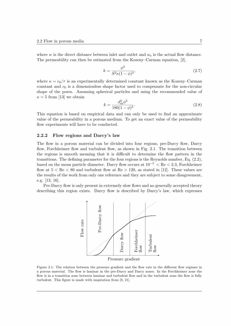
The flow in a porous material can be divided into four regions, pre-Darcy flow, Darcyflow, Forchheimer flow and turbulent flow, as shown in Fig. 2.1. The transition betweenthe regions is smooth meaning that it is difficult to determine the flow pattern in thetransitions. The defining parameter for the four regions is the Reynolds number, Eq. (2.2),based on the mean particle diameter. Darcy flow occurs at 10−5 < Re < 2.3, Forchheimerflow at 5 < Re < 80 and turbulent flow at Re > 120, as stated in [12]. These values arethe results of the work from only one reference and they are subject to some disagreement,e.g. [13, 16].
Pre-Darcy flow is only present in extremely slow flows and no generally accepted theorydescribing this region exists. Darcy flow is described by Darcy’s law, which expresses
Pre
-Darc
yflow
Darc
yflow
Forc
hhei
mer
flow
Turb
ule
nt
flow
Flo
wra
te
Pressure gradient
Figure 2.1: The relation between the pressure gradient and the flow rate in the different flow regimes ina porous material. The flow is laminar in the pre-Darcy and Darcy zones. In the Forchheimer zone theflow is in a transition zone between laminar and turbulent flow and in the turbulent zone the flow is fullyturbulent. This figure is made with inspiration from [8, 21].

8 CHAPTER 2. BASIC THEORY AND CONSIDERATIONS
a linearity between the permeating flow rate and the applied pressure difference, [2, 7,9]. Henry Darcy derived this law in 1856 from experiments with water through a pipecontaining sand, and it is given as
v = −k
η∇p, (2.9)
where v is the macroscopic velocity through the porous medium defined as v = Q/A withQ being the volume flow rate and A being the active surface area of the porous medium.The flow in the pre-Darcy and Darcy regions is laminar. When the inertial forces becomesignificant, the flow enters a transition zone between laminar and turbulent flow andDarcy’s law is no longer valid. The flow in the transition zone is denoted Forchheimerflow. When the flow enters the turbulent zone the flow is recognized as fully turbulentand it is then unstable and unsteady.
In membrane technology it is generally assumed that Darcy’s law is valid in the porousmedium. The following assumptions has to be valid in order to apply Darcy’s law, [2, 7, 9]:
• Inertial forces are negligible in the fluid flow.
• Isotropic porous medium. If it is anisotropic the permeability may vary in themedium.
• The pressure gradient is constant through the porous medium.
• The fluid is heterogeneous, i.e. the fluid has constant density.
• Completely saturated medium, i.e. there is a single fluid flow.
An estimate of a typical Reynolds number is made to determine whether or not it isreasonable to assume that the flow in SiC can be described by Darcy’s law. An estimateof the permeability of SiC is found to be k = 1× 10⁻¹³ m2 calculated from Eq. (2.8) witha porosity of φ = 0.4 and assuming that the mean grain diameter dm is approximatelythe same size as the mean pores, dm = 10 µm, see [20]. The dynamic viscosity of water at20C is η = 10−3 Pa s, a typical pressure difference is ∆p = 1bar and a typical thicknessof SiC is w = 2mm. The velocity in the porous SiC is found from Eq. (2.9) assuming thatthe pressure gradient is constant, ∇p = −∆p/w, giving a velocity of v = 5× 10⁻³ m/s.The Reynolds number is then found from Eq. (2.2) using this velocity and ρ = 1000 kg/m3
for water, to beRe ≈ 0.05. (2.10)
From this simple estimate the flow in the porous SiC can then be described by Darcy’slaw under typical conditions.
2.2.3 1D flow through porous plug in a pipe
A simple flow problem is used to find an analytical solution to the flow in a porous medium.The flow problem consists of an infinitely long, translation-invariant pipe with a plug ofporous material, see Fig. 2.2. The width of the plug is w while the radius of the pipe is
2.2 Flow in porous media 9
r
w
∆p + p∗
p∗
xr = 0
r = a
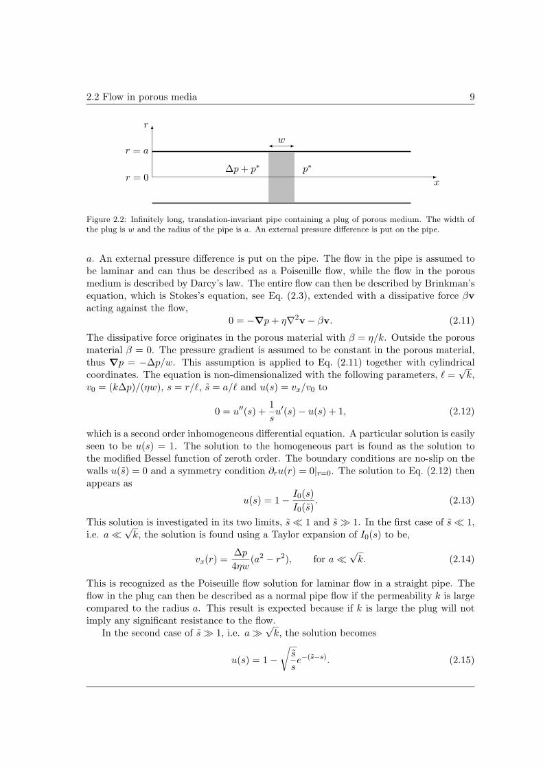
Figure 2.2: Infinitely long, translation-invariant pipe containing a plug of porous medium. The width ofthe plug is w and the radius of the pipe is a. An external pressure difference is put on the pipe.
a. An external pressure difference is put on the pipe. The flow in the pipe is assumed tobe laminar and can thus be described as a Poiseuille flow, while the flow in the porousmedium is described by Darcy’s law. The entire flow can then be described by Brinkman’sequation, which is Stokes’s equation, see Eq. (2.3), extended with a dissipative force βvacting against the flow,
0 = −∇p + η∇2v− βv. (2.11)
The dissipative force originates in the porous material with β = η/k. Outside the porousmaterial β = 0. The pressure gradient is assumed to be constant in the porous material,thus ∇p = −∆p/w. This assumption is applied to Eq. (2.11) together with cylindricalcoordinates. The equation is non-dimensionalized with the following parameters, ` =
√k,
v0 = (k∆p)/(ηw), s = r/`, s = a/` and u(s) = vx/v0 to
0 = u′′(s) +1su′(s)− u(s) + 1, (2.12)
which is a second order inhomogeneous differential equation. A particular solution is easilyseen to be u(s) = 1. The solution to the homogeneous part is found as the solution tothe modified Bessel function of zeroth order. The boundary conditions are no-slip on thewalls u(s) = 0 and a symmetry condition ∂ru(r) = 0|r=0. The solution to Eq. (2.12) thenappears as
u(s) = 1− I0(s)I0(s)
. (2.13)
This solution is investigated in its two limits, s ¿ 1 and s À 1. In the first case of s ¿ 1,i.e. a ¿
√k, the solution is found using a Taylor expansion of I0(s) to be,
vx(r) =∆p
4ηw(a2 − r2), for a ¿
√k. (2.14)
This is recognized as the Poiseuille flow solution for laminar flow in a straight pipe. Theflow in the plug can then be described as a normal pipe flow if the permeability k is largecompared to the radius a. This result is expected because if k is large the plug will notimply any significant resistance to the flow.
In the second case of s À 1, i.e. a À√
k, the solution becomes
u(s) = 1−√
s
se−(s−s). (2.15)
10 CHAPTER 2. BASIC THEORY AND CONSIDERATIONS
The permeability of SiC is around k = 1× 10⁻¹³ m2, and it is therefore a good approxi-mation to use u(s) ≡ 1. The velocity then becomes,
vx(r) = v0 =k
η
∆p
w, a À
√k, (2.16)
which is recognized as Darcy’s law in a 1D flow. From this it can be concluded that thevelocity in porous SiC can be described by Darcy’s law.
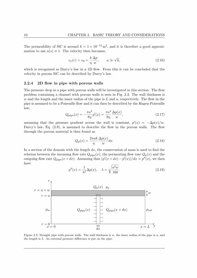
2.2.4 2D flow in pipe with porous walls
The pressure drop in a pipe with porous walls will be investigated in this section. The flowproblem containing a channel with porous walls is seen in Fig. 2.3. The wall thickness isw and the length and the inner radius of the pipe is L and a, respectively. The flow in thepipe is assumed to be a Poiseuille flow and it can then be described by the Hagen-Poiseuillelaw,
Qpipe(x) = −πa4
8ηp′(x) =
πa4
8η
∆p(x)w
, (2.17)
assuming that the pressure gradient across the wall is constant, p′(x) = −∆p(x)/w.Darcy’s law, Eq. (2.9), is assumed to describe the flow in the porous walls. The flowthrough the porous material is then found as
Qp(x) =2πak
η
∆p(x)w
dx. (2.18)
In a section of the domain with the length dx, the conservation of mass is used to find therelation between the incoming flow rate Qpipe(x), the permeating flow rate Qp(x) and theoutgoing flow rate Qpipe(x + dx). Assuming that (p′(x + dx)− p′(x))/dx = p′′(x), we thenhave
p′′(x) =1λ2
∆p(x), λ =
√a3w
16k. (2.19)
r
r = 0
r = a
r = a + w
xx = 0 x = L
w
dx
Qpipe(x) Qpipe(x + dx)
Qp(x)
pin pout
pp
Figure 2.3: Straight pipe with porous walls. The wall thickness is w, the inner radius of the pipe is a, andthe length is L. An external pressure difference is put on the pipe.

2.3 General channel flow 11
The solution to Eq. (2.19) must be an exponential function and since ∆p(x) = p(x)− pp
the solution has the following form,
p(x)− pp = Aex/λ + Be−x/λ. (2.20)
The boundary conditions are p(0) = pin and p(L) = pout as seen in Fig. 2.3. Using theseboundary conditions and pp = 0, the solution becomes
p(x) = pin +x
L
[pout − pin −
(L
λ
)2(13pin +
16pout
)]+
12
(x
λ
)2[pin
(1− 1
3x
L
)+
13pout
x
L
].
(2.21)It is seen that the factor (L/λ)2 controls the deviation from a linear pressure drop. Usinga = 6.5mm, w = 3.5mm, k = 1× 10⁻¹³ m2 and L = 305mm, we have (L/λ)2 = 2× 10⁻⁴ .Since (x/λ)2 ≤ (L/λ)2 ¿ 1, we can conclude that the pressure drop can be assumed tobe linear in a pipe with a laminar flow and walls of porous SiC. This means that thetransmembrane pressure ptm, which is the pressure difference over the porous wall of thepipe, can be estimated as
ptm =pin + pout
2− pp. (2.22)
This approximation of the transmembrane pressure will be used throughout this thesis.
2.3 General channel flow
In the previous section we assumed that the flow was laminar in the channel, but in manycases this is not true. When the Reynolds number exceeds 2300 the laminar channel flowbreaks down and when Re > 4000 the flow becomes fully turbulent, [3]. Pressure drops ina circular channel with viscous flow is described by the energy equation,
(p1
ρ+ α1
V 21
2+ gz1
)−
(p2
ρ+ α2
V 22
2+ gz2
)= hlT = hl + hlm , (2.23)
which assumes that the flow is steady and incompressible, and the internal energy and thepressure are uniformly distributed across the two cross-sections 1 and 2 in the channel.In Eq. (2.23) α is the kinetic energy coefficient, V is the average velocity in the channel,g is the gravitational constant and z is the vertical position. The subscripts 1 and 2corresponds to the cross-sections where the energy equation is applied. hlT is the totalhead loss and hl and hlm are the sum of the major and minor losses, respectively. The majorlosses are caused by the frictional effects in a straight channel with constant cross-section,while the minor losses are due to expansions, contractions, bends, inlets and outlets. Forfully developed flow through a horizontal pipe with constant cross-section we have thatα1V
21 /2 = α2V
22 /2 and hlm = 0 and Eq. (2.23) reduces to
p1 − p2
ρ=
∆p
ρ= hl. (2.24)
The major loss is found as
hl = fL
D
V 2
2, (2.25)

12 CHAPTER 2. BASIC THEORY AND CONSIDERATIONS
where f is the so-called friction factor, L the length between the two cross-sections and Dis the diameter of the channel. By combining Eqs. (2.24) and (2.25) a correlation betweenthe pressure difference and the flow rate appears,
∆p = Rc f(e
D,Re) Q2, Rc =
L
D5
8ρ
π2, (2.26)
where Rc is the channel resistance and e/D is the relative roughness in the pipe. Forlaminar flow, Re < 2300, the friction factor is defined as
f =64Re
. (2.27)
When inserting the laminar friction factor in Eq. (2.26), the Hagen-Poiseuille law for acircular straight channel appears,
∆p =128ηL
D4πQ. (2.28)
No analytical expression for the friction factor is known for turbulent flow, but it can beread from the experimentally based Moody diagram, e.g. [3], with known values of therelative roughness and the Reynolds number. Several mathematical expressions have beenfitted to the Moody diagram, the most widely used being the implicit expression fromColebrook,
1f0.5
= −2.0 log(
e/D
3.7+
2.51Re f0.5
). (2.29)
When assuming smooth channels, another fitted expression can be used in a turbulentflow at Re ≤ 105 called the Blasius correlation,
f =0.316Re0.25 (2.30)
Inserting the Blasius expression into Eq. (2.26) gives the turbulent relation between pres-sure drop and flow rate,
∆p =1.788Lη
14 ρ
34
D194 π
74
Q74 , (2.31)
and it is seen that the relation is nonlinear. Throughout this thesis we will use theColebrook expression, Eq. (2.29) in a turbulent flow as it is the more general of the twopresented here. Furthermore the SiC-tubes will be assumed to be smooth (e/D = 0), sincethe relative roughness is unknown.
We will thus use f = 64/Re in laminar flow at Re < 2300 and Colebrook with theassumption of smooth pipes is used at Re > 4000. In the transition zone between laminarand turbulent flow the friction factor is unknown and therefore a smooth transition ismade at 2300 ≤ Re ≤ 4000 between the laminar and the turbulent friction factor.

2.4 Equivalent circuit model 13
2.4 Equivalent circuit model
An analog between the Hagen-Poiseuille law, Eq. (2.28), and Ohm’s law in electricity isstudied. The Hagen-Poiseuille law is written more generally as
∆p = RhydQ, (2.32)
where Rhyd is the hydraulic resistance. This linear relation is compared to Ohm’s law,which states that
∆U = RI, (2.33)
where ∆U is the difference in electric potential difference, R is the electric resistance andI is the electric current. The analog between Eq. (2.32) and Eq. (2.33) is obvious andeven the rules of series/parallel coupling of resistors and capacitors can be used in theHagen-Poiseuille law. This means that for two channels in series coupling we can use thesimple additive law,
R = R1 + R2, (2.34)
and for two channels in parallel coupling we can use the additive law of inverse resistances,
R =(
1R1
+1
R2
)−1
=R1R2
R1 + R2. (2.35)
The analog can be used when building a numerical model of a fluidic network in whichthe pressure differences become electrical potential differences, the hydraulic channel re-sistances become resistors and flow rates become currents. For a given fluidic circuit ornetwork we can then apply Kirchhoff’s laws:
1. The sum of flow rates entering/leaving any node in the circuit is zero.
2. The sum of all pressure differences in any closed loop of the circuit is zero.
The analog between electrical and fluidic circuits is described in detail in [1].
2.5 The Laplace equation in 1D and 2D Darcy flow
The continuity equation for an incompressible fluid is given as
∇ · v = 0, (2.36)
and combining it with Darcy’s law from Eq. (2.9) the governing equation for the pressuredistribution in a porous medium appears,
∇2p = 0 (2.37)
which is the Laplace equation for the pressure. In a 1D flow problem through a porous plugwith thickness w and radius a, see Fig. 2.4(a), the solution to the pressure distribution isvery simple and found as
p(x) =p2 − p1
wx + p1, 0 ≤ x ≤ w. (2.38)
14 CHAPTER 2. BASIC THEORY AND CONSIDERATIONS
r
r = a1
r = a2
p1 p2x
w
p1 p2
r
r = a
r = 0
(a) (b)
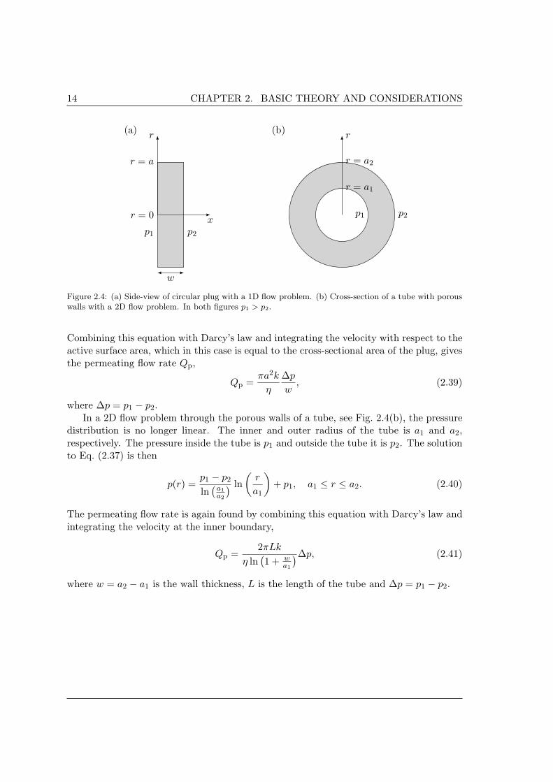
Figure 2.4: (a) Side-view of circular plug with a 1D flow problem. (b) Cross-section of a tube with porouswalls with a 2D flow problem. In both figures p1 > p2.
Combining this equation with Darcy’s law and integrating the velocity with respect to theactive surface area, which in this case is equal to the cross-sectional area of the plug, givesthe permeating flow rate Qp,
Qp =πa2k
η
∆p
w, (2.39)
where ∆p = p1 − p2.In a 2D flow problem through the porous walls of a tube, see Fig. 2.4(b), the pressure
distribution is no longer linear. The inner and outer radius of the tube is a1 and a2,respectively. The pressure inside the tube is p1 and outside the tube it is p2. The solutionto Eq. (2.37) is then
p(r) =p1 − p2
ln(
a1a2
) ln(
r
a1
)+ p1, a1 ≤ r ≤ a2. (2.40)
The permeating flow rate is again found by combining this equation with Darcy’s law andintegrating the velocity at the inner boundary,
Qp =2πLk
η ln(1 + w
a1
)∆p, (2.41)
where w = a2 − a1 is the wall thickness, L is the length of the tube and ∆p = p1 − p2.

Chapter 3
Fabrication and characterizationof SiC-samples
We fabricated all the SiC-monotubes and plugs, used throughout the experimental partof this thesis, from scratch starting with the SiC as a clay-like material delivered by thecompany LiqTech. This way we got a good feeling with SiC as a material and gainedinsight into the process of producing filters from SiC.
In the following we first describe the fabrication method used for the monotubes andplugs, and focus in particular on our own improvements leading to specimens of highquality. Second, we shortly present a few, simple characterization methods used to checkthe quality of the fabricated SiC-samples, and to estimate its porosity and average porediameter.
We are thankful to Johnny Marcher, technical director at LiqTech, for many goodadvice and technical discussions of SiC production methods. We are also grateful toAlexander Shapiro, associate professor, and Duc Thuong Vu, technician, both at theDepartment of Chemical and Biochemical Engineering, DTU, for introducing us to theComputed Tomography (CT) scanning method and for making the CT-scanner at theirdepartment available to us.
Specific comments about the fabrication process, like the composition of the SiC-material, the composition of the membranes and the sintering temperature have beenomitted, as it is confidential information.
3.1 Fabrication of SiC-plugs and tubes
This section appears a bit tedious, but the fabrication process is described in detail toshow how complicated it was to fabricate the high quality SiC-samples.
3.1.1 Plugs
The plugs were fabricated by mounting the SiC-clay between two pieces of paper in a press,and then pressing it into a flat plate shape, see Fig. 3.1. The paper was used to avoid
16 CHAPTER 3. FABRICATION AND CHARACTERIZATION OF SIC-SAMPLES
25 mm
1 2
3 4
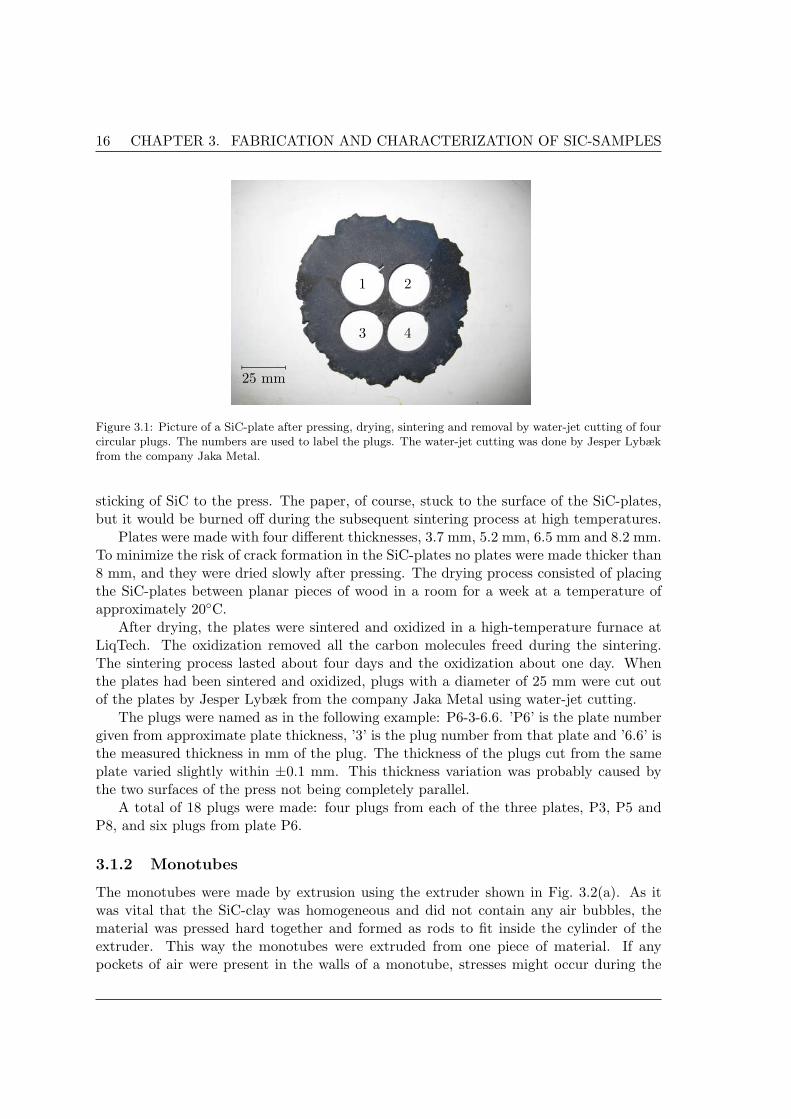
Figure 3.1: Picture of a SiC-plate after pressing, drying, sintering and removal by water-jet cutting of fourcircular plugs. The numbers are used to label the plugs. The water-jet cutting was done by Jesper Lybækfrom the company Jaka Metal.
sticking of SiC to the press. The paper, of course, stuck to the surface of the SiC-plates,but it would be burned off during the subsequent sintering process at high temperatures.
Plates were made with four different thicknesses, 3.7 mm, 5.2 mm, 6.5 mm and 8.2 mm.To minimize the risk of crack formation in the SiC-plates no plates were made thicker than8 mm, and they were dried slowly after pressing. The drying process consisted of placingthe SiC-plates between planar pieces of wood in a room for a week at a temperature ofapproximately 20C.
After drying, the plates were sintered and oxidized in a high-temperature furnace atLiqTech. The oxidization removed all the carbon molecules freed during the sintering.The sintering process lasted about four days and the oxidization about one day. Whenthe plates had been sintered and oxidized, plugs with a diameter of 25 mm were cut outof the plates by Jesper Lybæk from the company Jaka Metal using water-jet cutting.
The plugs were named as in the following example: P6-3-6.6. ’P6’ is the plate numbergiven from approximate plate thickness, ’3’ is the plug number from that plate and ’6.6’ isthe measured thickness in mm of the plug. The thickness of the plugs cut from the sameplate varied slightly within ±0.1 mm. This thickness variation was probably caused bythe two surfaces of the press not being completely parallel.
A total of 18 plugs were made: four plugs from each of the three plates, P3, P5 andP8, and six plugs from plate P6.
3.1.2 Monotubes
The monotubes were made by extrusion using the extruder shown in Fig. 3.2(a). As itwas vital that the SiC-clay was homogeneous and did not contain any air bubbles, thematerial was pressed hard together and formed as rods to fit inside the cylinder of theextruder. This way the monotubes were extruded from one piece of material. If anypockets of air were present in the walls of a monotube, stresses might occur during the
3.1 Fabrication of SiC-plugs and tubes 17
(a) (b)
Tube forair supply
Extruder↓ Air table
Mono-tube →
Air table
Extruder←
Air supply↑
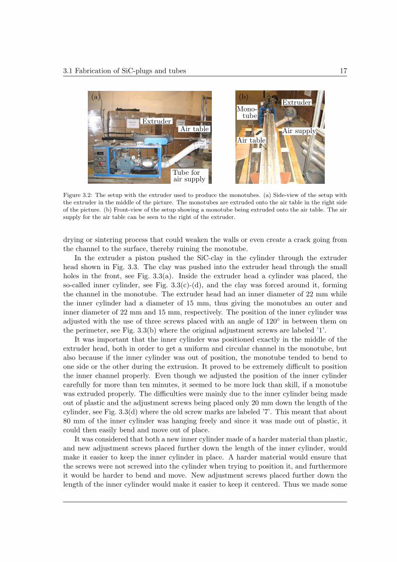
Figure 3.2: The setup with the extruder used to produce the monotubes. (a) Side-view of the setup withthe extruder in the middle of the picture. The monotubes are extruded onto the air table in the right sideof the picture. (b) Front-view of the setup showing a monotube being extruded onto the air table. The airsupply for the air table can be seen to the right of the extruder.
drying or sintering process that could weaken the walls or even create a crack going fromthe channel to the surface, thereby ruining the monotube.
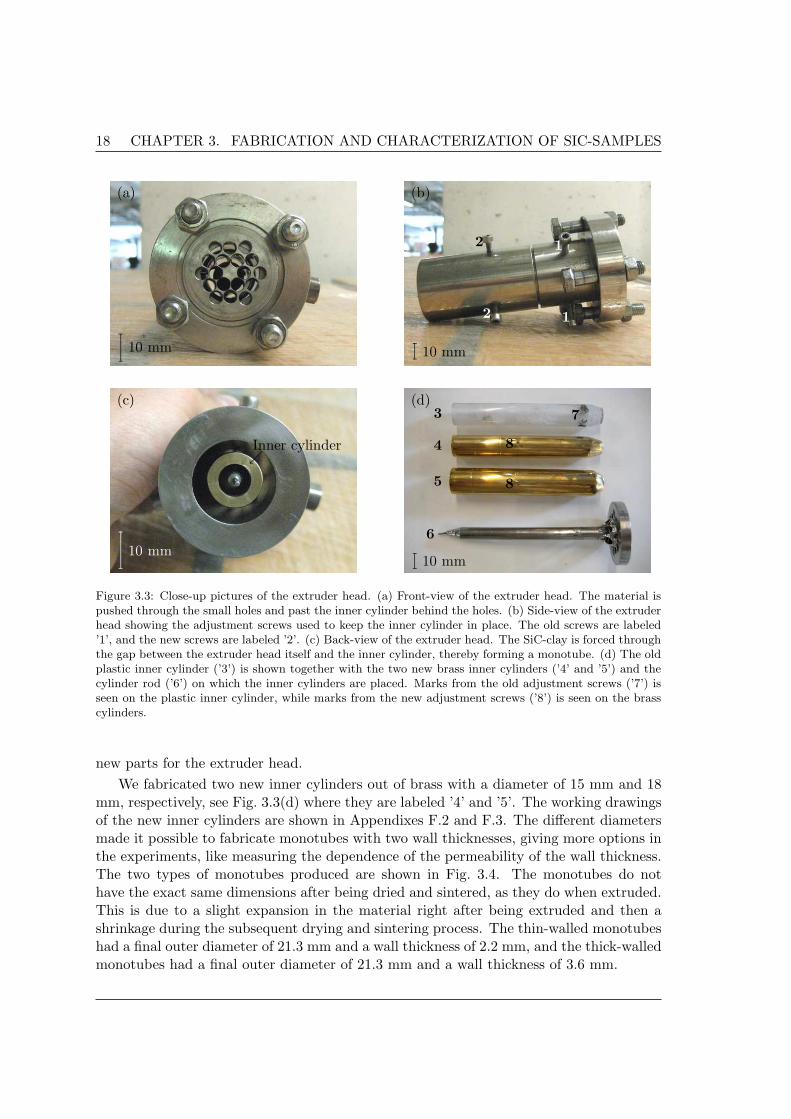
In the extruder a piston pushed the SiC-clay in the cylinder through the extruderhead shown in Fig. 3.3. The clay was pushed into the extruder head through the smallholes in the front, see Fig. 3.3(a). Inside the extruder head a cylinder was placed, theso-called inner cylinder, see Fig. 3.3(c)-(d), and the clay was forced around it, formingthe channel in the monotube. The extruder head had an inner diameter of 22 mm whilethe inner cylinder had a diameter of 15 mm, thus giving the monotubes an outer andinner diameter of 22 mm and 15 mm, respectively. The position of the inner cylinder wasadjusted with the use of three screws placed with an angle of 120 in between them onthe perimeter, see Fig. 3.3(b) where the original adjustment screws are labeled ’1’.
It was important that the inner cylinder was positioned exactly in the middle of theextruder head, both in order to get a uniform and circular channel in the monotube, butalso because if the inner cylinder was out of position, the monotube tended to bend toone side or the other during the extrusion. It proved to be extremely difficult to positionthe inner channel properly. Even though we adjusted the position of the inner cylindercarefully for more than ten minutes, it seemed to be more luck than skill, if a monotubewas extruded properly. The difficulties were mainly due to the inner cylinder being madeout of plastic and the adjustment screws being placed only 20 mm down the length of thecylinder, see Fig. 3.3(d) where the old screw marks are labeled ’7’. This meant that about80 mm of the inner cylinder was hanging freely and since it was made out of plastic, itcould then easily bend and move out of place.
It was considered that both a new inner cylinder made of a harder material than plastic,and new adjustment screws placed further down the length of the inner cylinder, wouldmake it easier to keep the inner cylinder in place. A harder material would ensure thatthe screws were not screwed into the cylinder when trying to position it, and furthermoreit would be harder to bend and move. New adjustment screws placed further down thelength of the inner cylinder would make it easier to keep it centered. Thus we made some
18 CHAPTER 3. FABRICATION AND CHARACTERIZATION OF SIC-SAMPLES
(a) (b)
(c) (d)
10 mm
1
1
2
2
10 mm
Inner cylinder
10 mm
3
4
5
6
7
8
8
10 mm
Figure 3.3: Close-up pictures of the extruder head. (a) Front-view of the extruder head. The material ispushed through the small holes and past the inner cylinder behind the holes. (b) Side-view of the extruderhead showing the adjustment screws used to keep the inner cylinder in place. The old screws are labeled’1’, and the new screws are labeled ’2’. (c) Back-view of the extruder head. The SiC-clay is forced throughthe gap between the extruder head itself and the inner cylinder, thereby forming a monotube. (d) The oldplastic inner cylinder (’3’) is shown together with the two new brass inner cylinders (’4’ and ’5’) and thecylinder rod (’6’) on which the inner cylinders are placed. Marks from the old adjustment screws (’7’) isseen on the plastic inner cylinder, while marks from the new adjustment screws (’8’) is seen on the brasscylinders.
new parts for the extruder head.We fabricated two new inner cylinders out of brass with a diameter of 15 mm and 18
mm, respectively, see Fig. 3.3(d) where they are labeled ’4’ and ’5’. The working drawingsof the new inner cylinders are shown in Appendixes F.2 and F.3. The different diametersmade it possible to fabricate monotubes with two wall thicknesses, giving more options inthe experiments, like measuring the dependence of the permeability of the wall thickness.The two types of monotubes produced are shown in Fig. 3.4. The monotubes do nothave the exact same dimensions after being dried and sintered, as they do when extruded.This is due to a slight expansion in the material right after being extruded and then ashrinkage during the subsequent drying and sintering process. The thin-walled monotubeshad a final outer diameter of 21.3 mm and a wall thickness of 2.2 mm, and the thick-walledmonotubes had a final outer diameter of 21.3 mm and a wall thickness of 3.6 mm.

3.1 Fabrication of SiC-plugs and tubes 19
(a) (b)
2.2 mm3.6 mm
Figure 3.4: Pictures of the cross-section of the two types of monotubes made with the improved extruder.(a) A thin-walled monotube with a wall thickness of 2.2 mm. (b) A thick-walled monotube with a wallthickness of 3.6 mm. Both monotubes have an outer diameter of 21.3 mm.
We also made a new part for the extruder head with new adjustment screws, see theworking drawing in Appendix F.1. In Fig. 3.3(b) the new adjustment screws are labeled’2’. The screws could not be placed too close to the end of the cylinder, since the SiC-clayhad to split to pass the screws and join on the other side. The screws were therefore placedabout 40 mm from the end of the extruder head. Furthermore the screws were made thinto prove as small an obstacle as possible.
During the extrusion of the monotubes it was important that the piston pushed theSiC-clay through the extruder head at the right speed. If it went too slow, the monotubesmight get an elliptical shape, before being put at the drying table. If it went too fast, theclay would not have time enough to join after passing the adjustment screws. Throughtrial-and-error we found the best speed of the piston to be approximately 12 cm/min whenextruding the thick-walled monotubes, and approximately 4 cm/min when extruding thethin-walled monotubes.
The monotubes were extruded out onto a table provided by LiqTech, the so-called airtable, shown in Fig. 3.2(b), with a channel formed as the bottom half of a cylinder. Aircould be blown out through small holes in the bottom of the channel, making the mono-tubes hover and reducing the friction significantly. Thereby the monotubes would not bedragged out of form during the extrusion. From the air table the monotubes were put intoaluminum pipes to keep them straight and then left to dry in a drying box. During thedrying process the aluminum pipes had to be turned often (at least every 2–3 minutes)so the monotubes kept their circular shape. In practice this was not doable, since thedrying process took several hours and we had to turn the pipes by hand. Therefore allthe monotubes dried this way got a slightly elliptical shape.
To avoid the monotubes getting an elliptical shape, LiqTech provided a table on whichthe aluminum pipes with the monotubes could be placed between two wheels and beturned at a constant velocity during the drying. Furthermore a fan was used to blow airthrough holes in a plate at the end of the table, see Fig. 3.5. By placing the aluminum

20 CHAPTER 3. FABRICATION AND CHARACTERIZATION OF SIC-SAMPLES
Aluminum pipes
Wheels
Holes for air flow
Figure 3.5: Table used to dry the extruded monotubes. The aluminum pipes were turned at a constantvelocity by the wheels while air was blown through the aluminum pipes in order to dry the monotubesfaster.
pipes in front of these holes, the drying time of the monotubes could be reduced. The airflow could not be too high, though, as cracks could appear in the monotubes if the surfacedried too fast compared to the middle of the walls. Through trial-and-error we found anappropriate air flow using tape at the inlet of the aluminum pipes. The tape was usedbecause the regulator for the fan was broken, setting the fan to maximum speed.
The monotubes dried faster upstream, since the air could absorb more moisture here.Further downstream less moisture could be absorbed due to the air becoming saturated,slowing the drying process. To optimize the drying process we turned the aluminum pipes180 every 30 minutes during the first three hours. Hereafter the pipes were turned onceevery hour until the monotubes were dry. The drying process lasted about five hours forthe thin-walled monotubes and eight hours for the thick-walled monotubes. Finally, thedried monotubes were sintered and oxidized in the same way as the plugs.
To sum up, the most important improvements we made to obtain the best possiblemonotubes are:
Monotubes extruded from one piece of material. The SiC-clay delivered by LiqTechwas formed as rods with a diameter and length to fit inside the cylinder of theextruder thereby minimizing the risk of air pocket formation in the walls of themonotubes during extrusion.
New adjustment screws for the extruder head. The original adjustment screws onthe extruder head were placed too close to the front, making it next to impossibleto center the inner cylinder accurately and it was easy to move the inner cylinderout of place. A new part for the extruder head was therefore made with adjustmentscrews placed closer to the end of the extruder head.
New inner cylinder made from a harder material. The original inner cylinder wasmade out of plastic. This meant that the adjustment screws could be screwed into
3.1 Fabrication of SiC-plugs and tubes 21
the surface of the cylinder, making it difficult to position it properly. Also the softplastic bend easily and moved during extrusion. Thus new inner cylinders were madeout of brass.
Improved drying table. During drying, the monotubes tended to get an elliptical shapeif they were not turned often for several hours. Thus a drying table was used onwhich the monotubes could be rotated at a constant velocity while drying.
Initially only the thick-walled monotubes could be made as only one inner cylinder wasavailable. The fabrication of the first three series of these monotubes was therefore used toimprove the fabrication method. In the experimental setup the monotubes had to have alength of 305 mm to fit the housing. Since the thick-walled monotubes could be extrudedto a length of about 500 mm from one piece of material, only one monotube could becut from each extruded length. The thick-walled monotubes were then named as in thefollowing example: IV-XV. ’IV’ is the number of the series and ’XV’ is the tube numberfrom that series.
The naming of the thin-walled monotubes was slightly different. The thinner wallsmeant that the monotubes could be extruded to a length of 1.1 m from one piece ofmaterial, which made it possible to get up to three monotubes with a length of 305 mmfrom each extruded length. One long monotube with a length of 1 m could also be cut,that fit in a long housing. Thus thin-walled monotubes with two different lengths weremade. The long thin-walled monotubes were named as in the following example: TI-XI. ’TI’ means it is a thin-walled tube from the first series and ’XI’ is the tube numberfrom that series. The short thin-walled monotubes were named as: TI-VI-II. ’TI’ againdescribes it as a thin-walled tube from the first series, ’VI’ is the tube number extrudedin that series and ’II’ is the number of the short monotube cut from that tube length.
We fabricated a total of 20 thick-walled monotubes, with 12 of these being of goodquality, in the final 4th series. All of these had a length of 305 mm, an outer diameter of21.3 mm and a wall thickness of 3.6 mm. 38 short and four long thin-walled monotubesof good quality were fabricated from a total of 23 extruded tubes. All of the thin-walledmonotubes have an outer diameter of 21.3 mm, and a wall thickness of 2.2 mm.
3.1.3 24-channel tubes
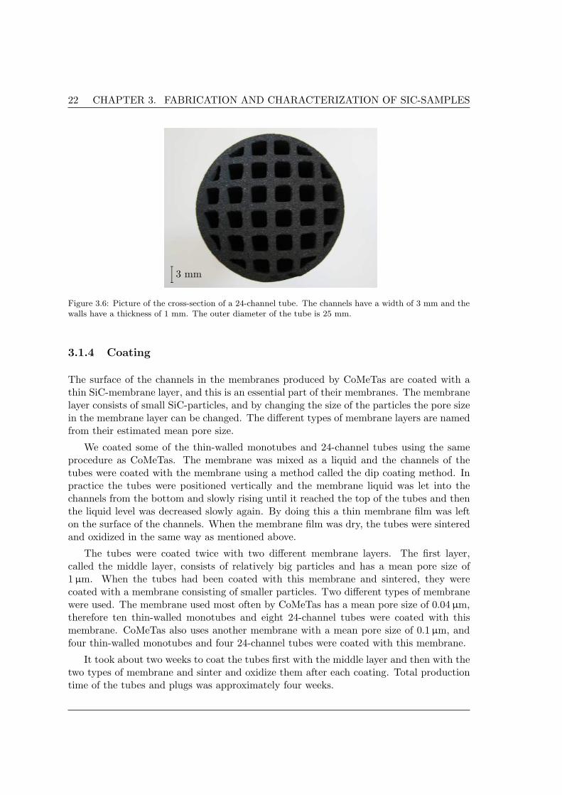
A set of tubes, called 24-channel tubes, containing many parallel channels was also fab-ricated, see Fig. 3.6. The channels are quadrilateral in shape and have a width of 3mm. There are 16 full channels in the middle of the design, while the outer channels, cutto follow the circular shape of the tube, combine to approximately 8 full channels, thusexplaining the name 24-channel tube. The walls have a thickness of 1 mm.
The 24-channel tubes are used in order to introduce a complex geometry in our exper-imental work that actually is used by CoMeTas in some of their membranes. It was notpossible to fabricate the 24-channel tubes with the extruder used for the monotubes andthey were instead fabricated by LiqTech. They were named as in the following example:XXIV-IV. ’XXIV’ denotes ”24-channel tube” and ’IV’ is the specific tube number. A totalof 20 24-channel tubes were fabricated, all of them having a length of 305 mm.
22 CHAPTER 3. FABRICATION AND CHARACTERIZATION OF SIC-SAMPLES
3 mm
Figure 3.6: Picture of the cross-section of a 24-channel tube. The channels have a width of 3 mm and thewalls have a thickness of 1 mm. The outer diameter of the tube is 25 mm.
3.1.4 Coating
The surface of the channels in the membranes produced by CoMeTas are coated with athin SiC-membrane layer, and this is an essential part of their membranes. The membranelayer consists of small SiC-particles, and by changing the size of the particles the pore sizein the membrane layer can be changed. The different types of membrane layers are namedfrom their estimated mean pore size.
We coated some of the thin-walled monotubes and 24-channel tubes using the sameprocedure as CoMeTas. The membrane was mixed as a liquid and the channels of thetubes were coated with the membrane using a method called the dip coating method. Inpractice the tubes were positioned vertically and the membrane liquid was let into thechannels from the bottom and slowly rising until it reached the top of the tubes and thenthe liquid level was decreased slowly again. By doing this a thin membrane film was lefton the surface of the channels. When the membrane film was dry, the tubes were sinteredand oxidized in the same way as mentioned above.
The tubes were coated twice with two different membrane layers. The first layer,called the middle layer, consists of relatively big particles and has a mean pore size of1µm. When the tubes had been coated with this membrane and sintered, they werecoated with a membrane consisting of smaller particles. Two different types of membranewere used. The membrane used most often by CoMeTas has a mean pore size of 0.04 µm,therefore ten thin-walled monotubes and eight 24-channel tubes were coated with thismembrane. CoMeTas also uses another membrane with a mean pore size of 0.1µm, andfour thin-walled monotubes and four 24-channel tubes were coated with this membrane.
It took about two weeks to coat the tubes first with the middle layer and then with thetwo types of membrane and sinter and oxidize them after each coating. Total productiontime of the tubes and plugs was approximately four weeks.

3.2 Characterization methods 23
3.2 Characterization methods
The characterization methods described here have been abridged, and only the most im-portant results are described.
3.2.1 CT-scan
We introduced the method of Computed Tomography scanning (CT-scanning) to CoMeTasin our studies of the homogeneity and quality of the porous SiC-tubes and plugs. CT-scanning is a medical imaging method, where digital geometry processing is used to gen-erate a three-dimensional image of the inside of an object from a large series of two-dimensional X-ray images taken around a single axis of rotation. A CT-scan producesa volume of data which can be manipulated, in order to demonstrate various structuresbased on their ability to block the X-ray beam. The CT-scanner can thus be used toverify, if the SiC-tubes and plugs are homogeneous, or if holes or cracks are present, andthereby we can determine if the tubes and plugs are of high or low quality.
Unfortunately the CT-scanner available to us broke down during the summer 2008 andwas not repaired before the end of our thesis work. Therefore we could not CT-scan theplugs and tubes used in our experimental work. However, we made some pictures of someof the thick-walled monotubes initially fabricated in our two first series of monotubes. ACT-picture of the cross-section of monotube II-V is shown in Fig. 3.7(a). The white areason the surface of the monotube arise, when the different pictures are combined. Inside ofthe white edges the porous material seems quite homogeneous, due to the uniform greycolor. If air in the form of a crack or hole is present in the material, it would appear as ablack area (like the channel in the tube). The so-called CT-number, which is an expressionof the amount of X-rays penetrating the object, can be used to determine, whether theobject contains cracks, holes, or any sort of impurities. In Fig. 3.7(b) a black area is clearlyseen in the upper region of the monotube. Judged from the color, this black area is mostlikely a hole in the material, which could either have been created during the extrusion,or when the tube was dried and subsequently sintered.
(a) (b)
3.6 mm 3.6 mm
Figure 3.7: (a) CT-picture of the cross-section of monotube II-V showing no sign of any holes or cracks.(b) Another CT-picture of II-V showing a hole in the upper region.
24 CHAPTER 3. FABRICATION AND CHARACTERIZATION OF SIC-SAMPLES
3.2.2 Porosity
The porosity φSiC of the SiC used in our plugs and tubes can be found from a simpleexperiment with the thin-walled and thick-walled monotubes, see Appendix A.1. We usedten thin-walled and eight thick-walled monotubes for this porosity experiment. The meanporosity, in %, of the SiC was found to be
φSiC = (38.2± 0.8)%, (3.1)
where the error is the standard deviation of the porosities found from each of the mono-tubes. A porosity of approximately 40% was expected for the SiC, and our results agreewell with these expectations.
3.2.3 Capillary rise
One way to determine the mean pore size dm of a porous medium, is by use of the capillaryrise method described in Appendix A.2. The contact angle θ at the water-SiC-air contactline is unknown, but as a rule of thumb it can be assumed to be θ = 0 for very hydrophilicmaterials. Three long monotubes were used for the capillary rise experiment and usingθ = 0 the average pore size was found to be approximately dm = 27µm which is nearlythree times higher than the expected pore size of around 10-12µm. The contact angleshould be more than 60 in order to obtain the expected average pore size in the porousmedia.
We made a small observation during the preliminary experiments concerning the cap-illary rise. Surprisingly, the first SiC-tubes we used showed no sign of water rise. Wediscovered that this was because the tubes had not been oxidized, and thus we found thatan easy way to see, if our tubes and plugs had been oxidized, was to check if they couldabsorb water.
3.2.4 Bubble point
The maximum pore size dmax as well as the homogeneity of our plugs and tubes, canbe found using the so-called bubble point method described in Appendix A.3. Using 13monotubes the average maximum pore diameter is found to be approximately 16µm, whena contact angle of θ = 0 is assumed. As mentioned, the mean pore diameter is expectedto be around 10-12µm, and it is expected that the maximum pore diameter is only slightlylarger. Thus, our results agree well with our expectations at a contact angle of θ = 0,opposed to the results found in the capillary rise method. The reason for this is unknownand has not been investigated further.
The bubble point test can be used not only for estimating the maximum pore diameter,but may also indicate if our plugs and tubes are damaged. If bubbles form at a lowerpressure than expected, and only in one region of the SiC-sample, it could indicate a holeor a crack in the sample.
Since the results from the capillary rise method and the bubble point method do notagree, no conclusions are made from the methods presented here. The methods are stillusable, however, as they give useful information concerning the quality of the SiC-samples.

Chapter 4
Experimental setup
The setup used for the experimental part of this thesis was provided by CoMeTas. It wasinstalled at the new premises of the company when our work was initiated. In the followingwe give a brief description of the setup and present only the most important informationrelevant for our work. In particular we focus on the thorough check and improvementswe had to make on this new setup to obtain satisfactory results. In total we spent twomonths of work to get the setup fully operational.
4.1 Description of the experimental setup
Basically the setup consists of four valves (V01–V04), one pump (P01), three adjustablevalves (AV01–AV03), two flow transmitters (FT01 and FT02), three pressure transmitters(PT01–PT03) and one temperature transmitter (TT01). The position of the differentparts on the experimental setup can be seen in the sketch of Fig. 4.1 and the pictures ofFig. 4.2. The specifications of the components are listed below.
Valves: 2/2-way angle seat valve, type 2000 DN 40 (Burkert Fluid Control Systems).
Pump: CRNE 5-16 multistage centrifugal pump with MGE 90 engine. 16-stage pumpwith nominal flow rate of 5.7m3/h (Grundfos).
Adjustable valves: Piston actuated angle seat valve, type 2702 DN 40, with side controlpositioner 1067 (Burkert Fluid Control Systems).
Flow transmitters: Sitrans F M Magflo electromagnetic flowmeter. Sensor type: MAG3100 HT, DN 40, with PTFE liner. Converter type: MAG 5000 IP 67. Measuringrange: 0 L/s – 2.5 L/s. Error from calibration report: ±0.09% at 90% of full-scaleflow; ±0.12% at 25% of full-scale flow (Siemens Instruments).
Pressure transmitters: Siemens Sitrans P, series Z. Measuring range of original trans-mitters: 0 bar – 16 bar. Measuring range of new transmitters1: two transmitters
1The new pressure transmitters will be discussed in Section 4.2

26 CHAPTER 4. EXPERIMENTAL SETUP
Feed
Clean water
Permeate
Retentate
P01V01
V02
AV01FT01
PT01
AV03
AV02
PT03
FT02V03
TT01PT02
V04
Back-flushtank
Housi
ng
Compressed air
Wate
rre
serv
oir
Figure 4.1: Diagram of the initial experimental setup containing four valves (V01–V04), a pump (P01),three adjustable valves (AV01–AV03), two flow transmitters (FT01 and FT02), three pressure transmitters(PT01–PT03) and a temperature transmitter (TT01). The plugs and tubes used in the experiments arepositioned in the housing. In a cross-flow setup the experimental setup is used as shown in this diagram,but when dead-end experiments are conducted the permeate flow is let out through the retentate exitin order to measure the temperature. Thus the permeate exit is not used in the dead-end setup. Thedemineralized water is recirculated in the water reservoir.
with range 0 bar – 4 bar and one with range 0 bar – 1.6 bar. Maximum error: ±0.5%of full-scale value (Siemens Instruments).
Temperature transmitter: Siemens Sitrans TF2. Measuring range: from -50C to+200C. Maximum error: ±0.5% of full-scale value (Siemens Instruments).
During the experiments the pump was used to control the feed pressure pf and thus the flowrate Q through the plugs and tubes. In the cross-flow experiments the adjustable valveson the retentate and permeate (AV02 and AV03, respectively) were used to control theretentate and permeate pressure (pr and pp, respectively) behind the tubes and thus theamount of flow coming through the retentate and permeate. The temperature transmittermeasures the temperature of the retentate flow when conduction cross-flow experiments,and in order to measure the fluid temperature in the dead-end setup, the permeate flowis let through the retentate exit in these experiments. Thus the permeate exit is not usedwhen conduction dead-end experiments. The dead-end and cross-flow setups are describedin Section 4.1.2. The valves and the pump are controlled directly on the experimentalsetup, using a control panel. All the data from the pump, valves and transmitters arelogged on a computer connected to a PLC-server on the experimental setup. The waterused in the experiments is recirculated in the water reservoir, labeled ’7’ in Fig. 4.2(a).It is led from the reservoir into the setup through the feed inlet (label ’6’ in Fig. 4.2(b))and out into the reservoir again through the retentate and permeate outlets (’4’ and ’5’,respectively, in Fig. 4.2(b)).
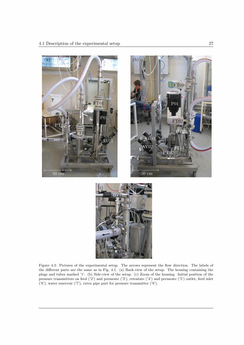
4.1 Description of the experimental setup 27
(a) (b)
(c)
1
1
1
P01
P01
AV01
AV02
AV03
FT01
FT01
FT02
FT02
2
3
PT01
PT01
PT03
PT03
PT02TT01
4
5
6
7
8
50 cm 50 cm
10 cm
Figure 4.2: Pictures of the experimental setup. The arrows represent the flow direction. The labels ofthe different parts are the same as in Fig. 4.1. (a) Back-view of the setup. The housing containing theplugs and tubes marked ’1’. (b) Side-view of the setup. (c) Zoom of the housing. Initial position of thepressure transmitters on feed (’2’) and permeate (’3’), retentate (’4’) and permeate (’5’) outlet, feed inlet(’6’), water reservoir (’7’), extra pipe part for pressure transmitter (’8’).
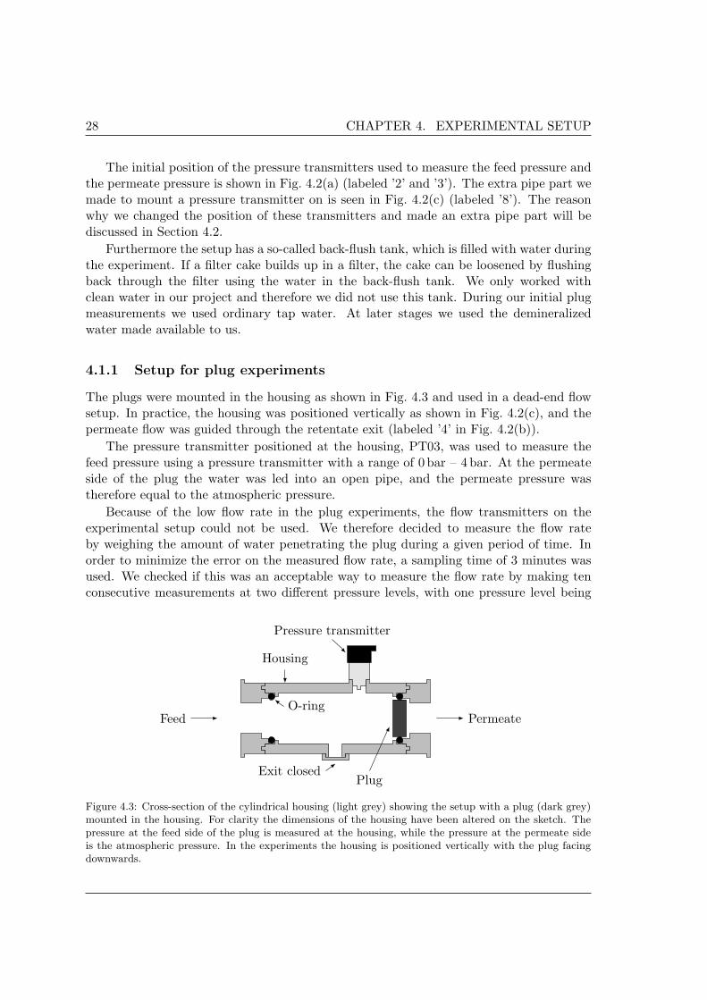
28 CHAPTER 4. EXPERIMENTAL SETUP
The initial position of the pressure transmitters used to measure the feed pressure andthe permeate pressure is shown in Fig. 4.2(a) (labeled ’2’ and ’3’). The extra pipe part wemade to mount a pressure transmitter on is seen in Fig. 4.2(c) (labeled ’8’). The reasonwhy we changed the position of these transmitters and made an extra pipe part will bediscussed in Section 4.2.
Furthermore the setup has a so-called back-flush tank, which is filled with water duringthe experiment. If a filter cake builds up in a filter, the cake can be loosened by flushingback through the filter using the water in the back-flush tank. We only worked withclean water in our project and therefore we did not use this tank. During our initial plugmeasurements we used ordinary tap water. At later stages we used the demineralizedwater made available to us.
4.1.1 Setup for plug experiments
The plugs were mounted in the housing as shown in Fig. 4.3 and used in a dead-end flowsetup. In practice, the housing was positioned vertically as shown in Fig. 4.2(c), and thepermeate flow was guided through the retentate exit (labeled ’4’ in Fig. 4.2(b)).
The pressure transmitter positioned at the housing, PT03, was used to measure thefeed pressure using a pressure transmitter with a range of 0 bar – 4 bar. At the permeateside of the plug the water was led into an open pipe, and the permeate pressure wastherefore equal to the atmospheric pressure.
Because of the low flow rate in the plug experiments, the flow transmitters on theexperimental setup could not be used. We therefore decided to measure the flow rateby weighing the amount of water penetrating the plug during a given period of time. Inorder to minimize the error on the measured flow rate, a sampling time of 3 minutes wasused. We checked if this was an acceptable way to measure the flow rate by making tenconsecutive measurements at two different pressure levels, with one pressure level being
Feed Permeate
Plug
O-ring
Housing
Exit closed
Pressure transmitter
Figure 4.3: Cross-section of the cylindrical housing (light grey) showing the setup with a plug (dark grey)mounted in the housing. For clarity the dimensions of the housing have been altered on the sketch. Thepressure at the feed side of the plug is measured at the housing, while the pressure at the permeate sideis the atmospheric pressure. In the experiments the housing is positioned vertically with the plug facingdownwards.

4.1 Description of the experimental setup 29
in the low end of the measuring range and the other in the high end. The maximumdeviation from the mean value at the two pressure levels was 3%.
The plugs were mounted in the housing with an O-ring and it was made sure that nowater passed the plugs without going through them. We checked this by making two plugsimpermeable with glue. The plugs were then put in the housing and the pressure increasedup to our maximum pressure of 4 bar. No leakages were observed and we concluded thatthe sealing of the plugs was tight.
4.1.2 Setup for tube experiments
The monotubes and the 24-channel tubes were mounted with O-rings in the housing inmuch the same way as the plugs as shown in Fig. 4.4. A pressure transmitter with a rangeof 0 bar – 1.6 bar was used to measure the permeate pressure at the housing.
Cross-flow setup
In the cross-flow experiments the setup was used as shown in Fig. 4.2. The extra pipepart was mounted just before the housing and the feed pressure was measured here usingthe pressure transmitter called PT01. The retentate pressure was measured using PT02after the housing. Both PT01 and PT02 had a range of 0 bar – 4 bar. As Fig. 4.2(b)shows, PT02 is positioned slightly below the housing and therefore measures a too highpressure due to the hydrostatic pressure implied by the height difference. During thedata processing we compensated for the hight difference to get the pressure just after thehousing.
The feed flow rate Qf was measured using FT01 while the permeate flow rate Qp wasmeasured using FT02. The retentate flow rate Qr could then be calculated as Qr = Qf−Qp.
Feed Retentate
Permeate
SiC tube
O-ringHousing
Pressure transmitter
Figure 4.4: Cross-section of the cylindrical housing (light grey) showing the setup with a tube (dark grey)mounted in the housing. For clarity the dimensions of the housing have been altered on the sketch. Thepressure transmitter mounted at the housing is used to measure the permeate pressure.
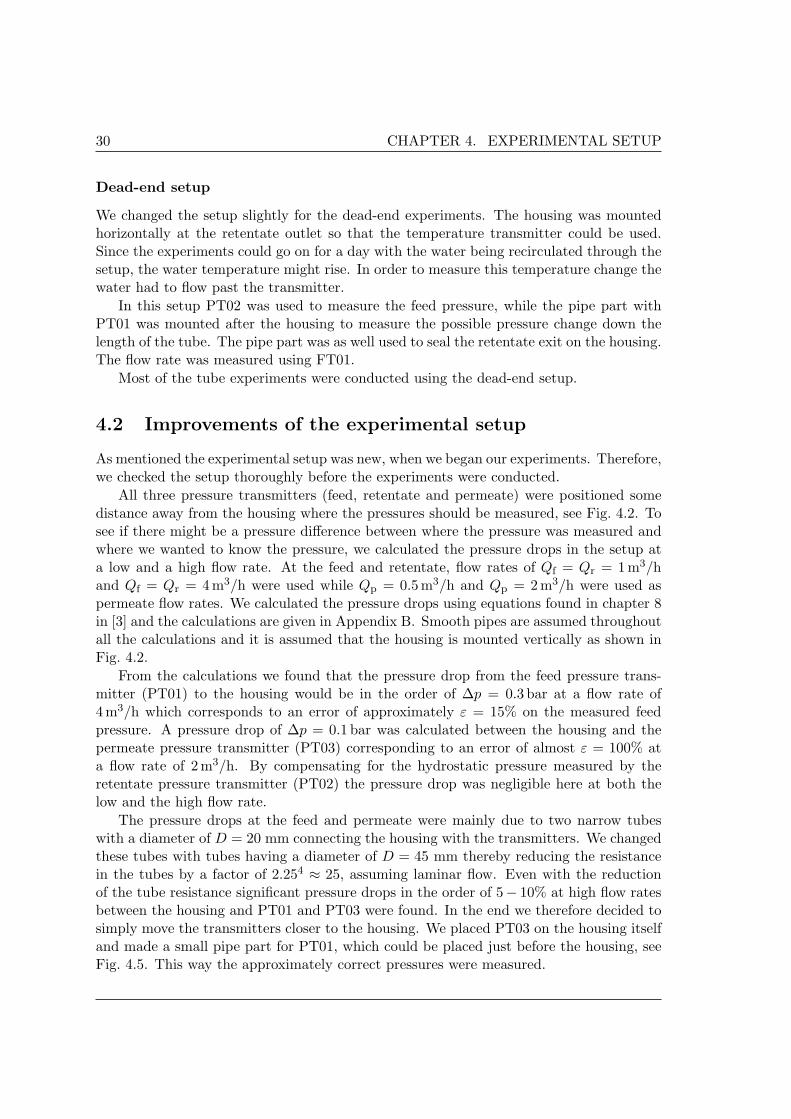
30 CHAPTER 4. EXPERIMENTAL SETUP
Dead-end setup
We changed the setup slightly for the dead-end experiments. The housing was mountedhorizontally at the retentate outlet so that the temperature transmitter could be used.Since the experiments could go on for a day with the water being recirculated through thesetup, the water temperature might rise. In order to measure this temperature change thewater had to flow past the transmitter.
In this setup PT02 was used to measure the feed pressure, while the pipe part withPT01 was mounted after the housing to measure the possible pressure change down thelength of the tube. The pipe part was as well used to seal the retentate exit on the housing.The flow rate was measured using FT01.
Most of the tube experiments were conducted using the dead-end setup.
4.2 Improvements of the experimental setup
As mentioned the experimental setup was new, when we began our experiments. Therefore,we checked the setup thoroughly before the experiments were conducted.
All three pressure transmitters (feed, retentate and permeate) were positioned somedistance away from the housing where the pressures should be measured, see Fig. 4.2. Tosee if there might be a pressure difference between where the pressure was measured andwhere we wanted to know the pressure, we calculated the pressure drops in the setup ata low and a high flow rate. At the feed and retentate, flow rates of Qf = Qr = 1 m3/hand Qf = Qr = 4m3/h were used while Qp = 0.5m3/h and Qp = 2 m3/h were used aspermeate flow rates. We calculated the pressure drops using equations found in chapter 8in [3] and the calculations are given in Appendix B. Smooth pipes are assumed throughoutall the calculations and it is assumed that the housing is mounted vertically as shown inFig. 4.2.
From the calculations we found that the pressure drop from the feed pressure trans-mitter (PT01) to the housing would be in the order of ∆p = 0.3 bar at a flow rate of4m3/h which corresponds to an error of approximately ε = 15% on the measured feedpressure. A pressure drop of ∆p = 0.1 bar was calculated between the housing and thepermeate pressure transmitter (PT03) corresponding to an error of almost ε = 100% ata flow rate of 2 m3/h. By compensating for the hydrostatic pressure measured by theretentate pressure transmitter (PT02) the pressure drop was negligible here at both thelow and the high flow rate.
The pressure drops at the feed and permeate were mainly due to two narrow tubeswith a diameter of D = 20 mm connecting the housing with the transmitters. We changedthese tubes with tubes having a diameter of D = 45 mm thereby reducing the resistancein the tubes by a factor of 2.254 ≈ 25, assuming laminar flow. Even with the reductionof the tube resistance significant pressure drops in the order of 5− 10% at high flow ratesbetween the housing and PT01 and PT03 were found. In the end we therefore decided tosimply move the transmitters closer to the housing. We placed PT03 on the housing itselfand made a small pipe part for PT01, which could be placed just before the housing, seeFig. 4.5. This way the approximately correct pressures were measured.
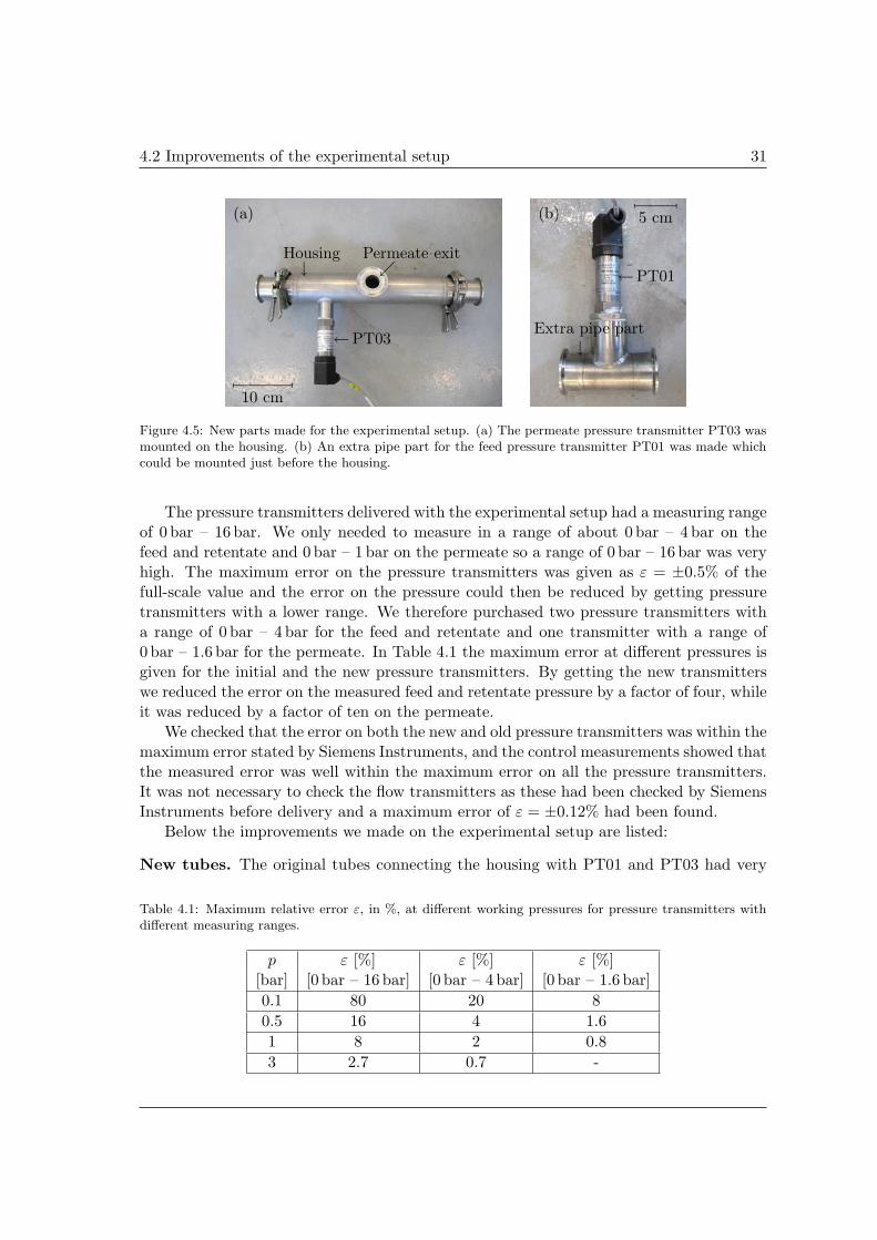
4.2 Improvements of the experimental setup 31
(a) (b)
10 cm
↓Housing
←PT03
Permeate exit
↓
Extra pipe part
5 cm
←PT01
Figure 4.5: New parts made for the experimental setup. (a) The permeate pressure transmitter PT03 wasmounted on the housing. (b) An extra pipe part for the feed pressure transmitter PT01 was made whichcould be mounted just before the housing.
The pressure transmitters delivered with the experimental setup had a measuring rangeof 0 bar – 16 bar. We only needed to measure in a range of about 0 bar – 4 bar on thefeed and retentate and 0 bar – 1 bar on the permeate so a range of 0 bar – 16 bar was veryhigh. The maximum error on the pressure transmitters was given as ε = ±0.5% of thefull-scale value and the error on the pressure could then be reduced by getting pressuretransmitters with a lower range. We therefore purchased two pressure transmitters witha range of 0 bar – 4 bar for the feed and retentate and one transmitter with a range of0 bar – 1.6 bar for the permeate. In Table 4.1 the maximum error at different pressures isgiven for the initial and the new pressure transmitters. By getting the new transmitterswe reduced the error on the measured feed and retentate pressure by a factor of four, whileit was reduced by a factor of ten on the permeate.
We checked that the error on both the new and old pressure transmitters was within themaximum error stated by Siemens Instruments, and the control measurements showed thatthe measured error was well within the maximum error on all the pressure transmitters.It was not necessary to check the flow transmitters as these had been checked by SiemensInstruments before delivery and a maximum error of ε = ±0.12% had been found.
Below the improvements we made on the experimental setup are listed:
New tubes. The original tubes connecting the housing with PT01 and PT03 had very
Table 4.1: Maximum relative error ε, in %, at different working pressures for pressure transmitters withdifferent measuring ranges.
p ε [%] ε [%] ε [%][bar] [0 bar – 16 bar] [0 bar – 4 bar] [0 bar – 1.6 bar]0.1 80 20 80.5 16 4 1.61 8 2 0.83 2.7 0.7 -
32 CHAPTER 4. EXPERIMENTAL SETUP
small diameters. We acquired new tubes with a larger diameter which reduced thepressure drop in the tubes by a factor of approximately 25, assuming laminar flowand constant velocity.
Changed position of PT01 and PT03. PT01 and PT03 were placed too far from thehousing, thus they did not measure the correct pressures. We changed their positionand mounted PT03 on the housing while an extra pipe part was made for PT01which could be mounted in front of the housing.
New pressure transmitters. The initial pressure transmitters had a too high measur-ing range of 0 bar – 16 bar which resulted in an unacceptable high error in the usedmeasuring range. We purchased two new pressure transmitters for the feed and re-tentate with a range of 0 bar – 4 bar and one for the permeate with a range of 0 bar– 1.6 bar. Thus we reduced the error on the measured feed and retentate pressureby a factor of four and on the permeate pressure by a factor of ten.

Chapter 5
Experiments with SiC-substrates
In the following we first present our experiments with the simple SiC-plugs of four differentthicknesses followed by the monotubes of two different wall thicknesses. The purpose ofthese experiments is to confirm Darcy’s law for flow in porous materials, to find thepermeability of the porous SiC, and to investigate if the permeability is independent ofthe thickness of the SiC.
Second we present our experiments with the 24-channel tubes. The goal is to getsome experimental data with a more complicated geometry which can be compared to theresults from our simulations and thereby verify our numerical models.
The experiments in this chapter represent two months of experimental work. Duringthe plug experiments, three weeks were used to solve some encountered problems regardingcontamination of our plug samples. We are thankful to Jørgen Wagner, senior applicationmanager at CoMeTas, for discussions of the contamination problems, and for his goodadvice on how to solve them.
5.1 Plugs
The simplest way to measure the permeability of the porous SiC and to verify Darcy’slaw, was to make a plug out of SiC and force the water flow through it, i.e. use the plugas a dead-end filter. A 1D flow can then be assumed in the plug, and Darcy’s law is givenfrom Eq. (2.16). Assuming 1D flow in the plugs the permeating flow rate Qp can be foundfrom Eq. (2.39). Rewriting this equation slightly gives
Qp =πd2k
4ηwptm, (5.1)
where d is the diameter of the plug and ptm = pf − pp is the transmembrane pressurewith pf being the feed pressure and pp the permeate pressure. The pressures are givenas gauge pressures. The flow rate and the pressure are measured during the experiments,while η, d and w are known values. Thus, k can be found from Eq. (5.1). As mentioned inChapter 4, ordinary tap water is used in the plug experiments since demineralized waterwas unavailable at the time the experiments were conducted. The water was kept at 20C
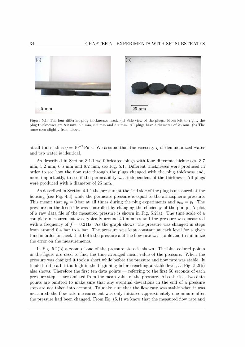
34 CHAPTER 5. EXPERIMENTS WITH SIC-SUBSTRATES
(a) (b)
5 mm 25 mm
Figure 5.1: The four different plug thicknesses used. (a) Side-view of the plugs. From left to right, theplug thicknesses are 8.2 mm, 6.5 mm, 5.2 mm and 3.7 mm. All plugs have a diameter of 25 mm. (b) Thesame seen slightly from above.
at all times, thus η = 10−3 Pa s. We assume that the viscosity η of demineralized waterand tap water is identical.
As described in Section 3.1.1 we fabricated plugs with four different thicknesses, 3.7mm, 5.2 mm, 6.5 mm and 8.2 mm, see Fig. 5.1. Different thicknesses were produced inorder to see how the flow rate through the plugs changed with the plug thickness and,more importantly, to see if the permeability was independent of the thickness. All plugswere produced with a diameter of 25 mm.
As described in Section 4.1.1 the pressure at the feed side of the plug is measured at thehousing (see Fig. 4.3) while the permeate pressure is equal to the atmospheric pressure.This meant that pp = 0 bar at all times during the plug experiments and ptm = pf. Thepressure on the feed side was controlled by changing the efficiency of the pump. A plotof a raw data file of the measured pressure is shown in Fig. 5.2(a). The time scale of acomplete measurement was typically around 40 minutes and the pressure was measuredwith a frequency of f = 0.2Hz. As the graph shows, the pressure was changed in stepsfrom around 0.4 bar to 4 bar. The pressure was kept constant at each level for a giventime in order to check that both the pressure and the flow rate was stable and to minimizethe error on the measurements.
In Fig. 5.2(b) a zoom of one of the pressure steps is shown. The blue colored pointsin the figure are used to find the time averaged mean value of the pressure. When thepressure was changed it took a short while before the pressure and flow rate was stable. Ittended to be a bit too high in the beginning before reaching a stable level, as Fig. 5.2(b)also shows. Therefore the first ten data points — referring to the first 50 seconds of eachpressure step — are omitted from the mean value of the pressure. Also the last two datapoints are omitted to make sure that any eventual deviations in the end of a pressurestep are not taken into account. To make sure that the flow rate was stable when it wasmeasured, the flow rate measurement was only initiated approximately one minute afterthe pressure had been changed. From Eq. (5.1) we know that the measured flow rate and
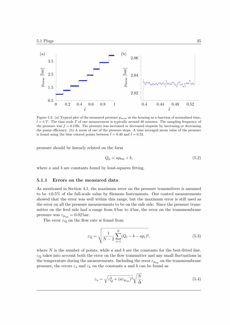
5.1 Plugs 35
(a) (b)
0 0.2 0.4 0.6 0.8 10.5
1.5
2.5
3.5
t
pm
eas
[bar
]
0.4 0.44 0.48 0.52
2.02
2.04
2.06
t
pm
eas
[bar
]
Figure 5.2: (a) Typical plot of the measured pressure pmeas at the housing as a function of normalized time,t = t/T . The time scale T of one measurement is typically around 40 minutes. The sampling frequency ofthe pressure was f = 0.2Hz. The pressure was increased or decreased stepwise by increasing or decreasingthe pump efficiency. (b) A zoom of one of the pressure steps. A time averaged mean value of the pressureis found using the blue colored points between t = 0.40 and t = 0.53.
pressure should be linearly related on the form
Qp = aptm + b, (5.2)
where a and b are constants found by least-squares fitting.
5.1.1 Errors on the measured data
As mentioned in Section 4.1, the maximum error on the pressure transmitters is assumedto be ±0.5% of the full-scale value by Siemens Instruments. Our control measurementsshowed that the error was well within this range, but the maximum error is still used asthe error on all the pressure measurements to be on the safe side. Since the pressure trans-mitter on the feed side had a range from 0 bar to 4 bar, the error on the transmembranepressure was εptm
= 0.02 bar.The error εQ on the flow rate is found from
εQ =
√√√√ 1N − 2
N∑
i=1
(Qi − b− api)2, (5.3)
where N is the number of points, while a and b are the constants for the best-fitted line.εQ takes into account both the error on the flow transmitter and any small fluctuations inthe temperature during the measurements. Including the error εptm
on the transmembranepressure, the errors εa and εb on the constants a and b can be found as
εa =√
ε2Q + (aεptm
)2√
N
∆, (5.4)
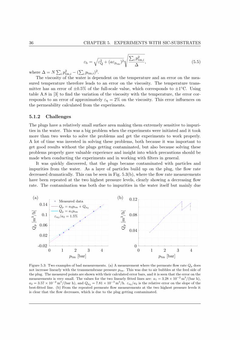
36 CHAPTER 5. EXPERIMENTS WITH SIC-SUBSTRATES
εb =√
ε2Q + (aεptm
)2
√∑i p
2tm,i
∆, (5.5)
where ∆ = N∑
i p2tm,i − (
∑i ptm,i)2.
The viscosity of the water is dependent on the temperature and an error on the mea-sured temperature therefore leads to an error on the viscosity. The temperature trans-mitter has an error of ±0.5% of the full-scale value, which corresponds to ±1C. Usingtable A.8 in [3] to find the variation of the viscosity with the temperature, the error cor-responds to an error of approximately εη = 2% on the viscosity. This error influences onthe permeability calculated from the experiments.
5.1.2 Challenges
The plugs have a relatively small surface area making them extremely sensitive to impuri-ties in the water. This was a big problem when the experiments were initiated and it tookmore than two weeks to solve the problems and get the experiments to work properly.A lot of time was invested in solving these problems, both because it was important toget good results without the plugs getting contaminated, but also because solving theseproblems properly gave valuable experience and insight into which precautions should bemade when conducting the experiments and in working with filters in general.
It was quickly discovered, that the plugs became contaminated with particles andimpurities from the water. As a layer of particles build up on the plug, the flow ratedecreased dramatically. This can be seen in Fig. 5.3(b), where the flow rate measurementshave been repeated at the two highest pressure levels, clearly showing a decreasing flowrate. The contamination was both due to impurities in the water itself but mainly due
(a)
(b)
-0.02
0.02
0.06
0.1
0.14
0 1 2 3 4
Qp
[m3/h
]
ptm [bar]
0
0.04
0.08
0.12
0 1 2 3 4
Qp
[m3/h
]
ptm [bar]
x Measured data
Qp = a2ptm + Qp2
Qp = a1ptm
εa2/a2 = 1.5%
Figure 5.3: Two examples of bad measurements. (a) A measurement where the permeate flow rate Qp doesnot increase linearly with the transmembrane pressure ptm. This was due to air bubbles at the feed side ofthe plug. The measured points are shown with their calculated error bars, and it is seen that the error on themeasurements is very small. The values for the two linearly fitted lines are: a1 = 3.28× 10⁻² m3/(bar h),a2 = 3.57× 10⁻² m3/(bar h), and Qp2 = 7.81× 10⁻³ m3/h. εa2/a2 is the relative error on the slope of thebest-fitted line. (b) From the repeated permeate flow measurements at the two highest pressure levels itis clear that the flow decreases, which is due to the plug getting contaminated.
5.1 Plugs 37
to impurities in the experimental setup. The setup had been used for some kind of oilsolution that stuck to the inside of the tubes and pipes. During the experiments this oilsolution was carried with the water and stuck to the surface of the plugs. A lot of time wasused to clean the setup with everything from normal soap to chlorine and finally a verystrong cleaning detergent, Divos 120CL from JohnsonDiversey, which proved successful.Even though the setup was cleaned thoroughly, the plugs were so sensitive, that just atiny amount of impurities could be seen as a decrease in the flow rate. Therefore the finalsolution was to use a filter borrowed from CoMeTas to pre-filter the water before the plug.
The low flow rate meant that air could be present in the setup during the measure-ments. We observed, that if a plug was put in the housing and an experiment startedfrom low pressure, air bubbles could influence the flow rate at the low pressures, so that alower flow rate than expected was measured. As the pressure was increased, the air bub-bles would disappear as they were pressed through the plug, giving a nonlinear relationbetween Qp and ptm. An example of such a measurement is shown in Fig. 5.3(a). Twolines have been fitted to the data points, one is forced through (0, 0) while the other isthe best linear fit. These two lines should ideally be the same, but due to the nonlinearrelation they are not. The solution to the air problem was to increase the pressure to themaximum pressure of 4 bar to get the air bubbles out of the setup and then lower thepressure again before the measurements were begun.
As mentioned above, normal tap water was used in the plug experiments. When aplug had been used for an experiment and then dried, limescale became a problem in thepores of the plugs making it impossible to repeat a measurement. At first chlorine wasused to try and solve this problem but it did not restore the flow rate to the state of theinitial measurements. Our solution was citric acid since it dissolves the limescale better,making it easy to get it out of the pores in the plugs.
Bacteria growth in the water also became a problem during the experiments. If thewater had been standing in the setup overnight the plugs would get contaminated bybacteria, called biofouling. The biofouling could be seen as a translucent, sticky film lyingon the surface of the plugs. As it was not desirable to change the water in the setup everyday, we decided to eliminate the bacteria using chlorine in the water. However, it wassoon discovered that the chlorine reacted with the pipe weldings in the setup, making rustin the water a problem. The chlorine could react with the weldings because they had notbeen made from a stainless alloy. We solved this problem using nitric acid in the waterinstead of chlorine. This had two major effects: The nitric acid lowered the pH valuethereby killing the bacteria and it dissolved the rust in the pipes created by the chlorine.Furthermore, it dissolved the limescale just as good as the citric acid. Three problemswere thus solved using nitric acid in the water. Throughout all the experiments nitric acidwas therefore used in the water to lower the pH value to approximately 3. It is assumedthat the use of nitric acid does not change the viscosity significantly since the viscosity ofnitric acid is close to that of water and only around 200 mL of nitric acid is used in 70 Lof water.
To sum up the encountered problems together with our solutions are listed below:
Particles/impurities in the water and setup: This was solved using a strong clean-

38 CHAPTER 5. EXPERIMENTS WITH SIC-SUBSTRATES
ing detergent, Divos 120CL from JohnsonDiversey, to clean the setup and thenpre-filter the water before the plug with a filter borrowed from CoMeTas.
Air in the setup: We increased the pressure to the maximum pressure used during theplug experiments of 4 bar and then lowered it again before an experiment was begun.This way the air was removed from the setup.
Limescale: Citric acid was used as it dissolved the limescale completely making it possibleto remove the limescale from the pores of the plugs. Later we used nitric acid withequally good results.
Biofouling: Bacteria growth in the water resulting in biofouling of the plugs was elimi-nated by lowering the pH value of the water to approximately 3 using nitric acid.
Rust: Rust in the setup due to chlorine reacting with the weldings was dissolved usingnitric acid in the water.
5.1.3 Results
During the experiments with the different plugs the repeatability of the measurementswas checked in several ways. The pressure was both increased and decreased to see if anyhysteresis effect could be seen, the plugs were taken out of the housing and put in again,they were turned around in the housing, they were left to dry for several days and finallythey were left in the setup during a weekend. None of these checks showed any deviationsin the measurements. It was also checked several times if the plugs got contaminated.This was done by keeping the pressure level constant for at least an hour and measure theflow rate in the beginning and in the end of this hour.
In Fig. 5.4 a plot is shown of four measurements made with the same plug, P5-1-5.2. The four measurements lie very close together showing good repeatability of theexperiments. The error bars on the measured points and the relative error for the bestlinear fit εa2/a2 have been calculated as described in Section 5.1.1, and it is clear that theerror on the experimental method is insignificant.
In measurement one and three the pressure was increased, while it was decreased inmeasurement two and four. From this it can be concluded that no hysteresis effect isfound. Eight points were made in each of the four measurements giving a total of 32points in the plot. Three different lines have been fitted to the points; the cyan coloredis a linear fit forced through (0, 0), the magenta is the best linear fit and the green is asecond order fit. From Darcy’s law a linear relationship going through (0, 0) is expectedbetween Qp and ptm. The three fitted lines confirm that this is the case. The two linearfits have the same slope of a1 = a2 = 4.32× 10⁻² m3/(h bar) and the intersection with theQ-axis of the best linear fit, Qp2
= 1× 10⁻⁴ m3/h, is effectively zero, since the calculatederror is εQp2
= 6× 10⁻⁴ m3/h.The second order fit is suppressed to a linear fit, which can be seen by compar-
ing the second order term, b3 = −4.7× 10⁻⁴ m3/(h bar2), with the linear term, a3 =4.54× 10⁻² m3/(h bar). Since ptm is in the order of 1 bar to 4 bar, b3ptm is roughly twoorders of magnitude lower than a3, making it redundant in the expression. Furthermore
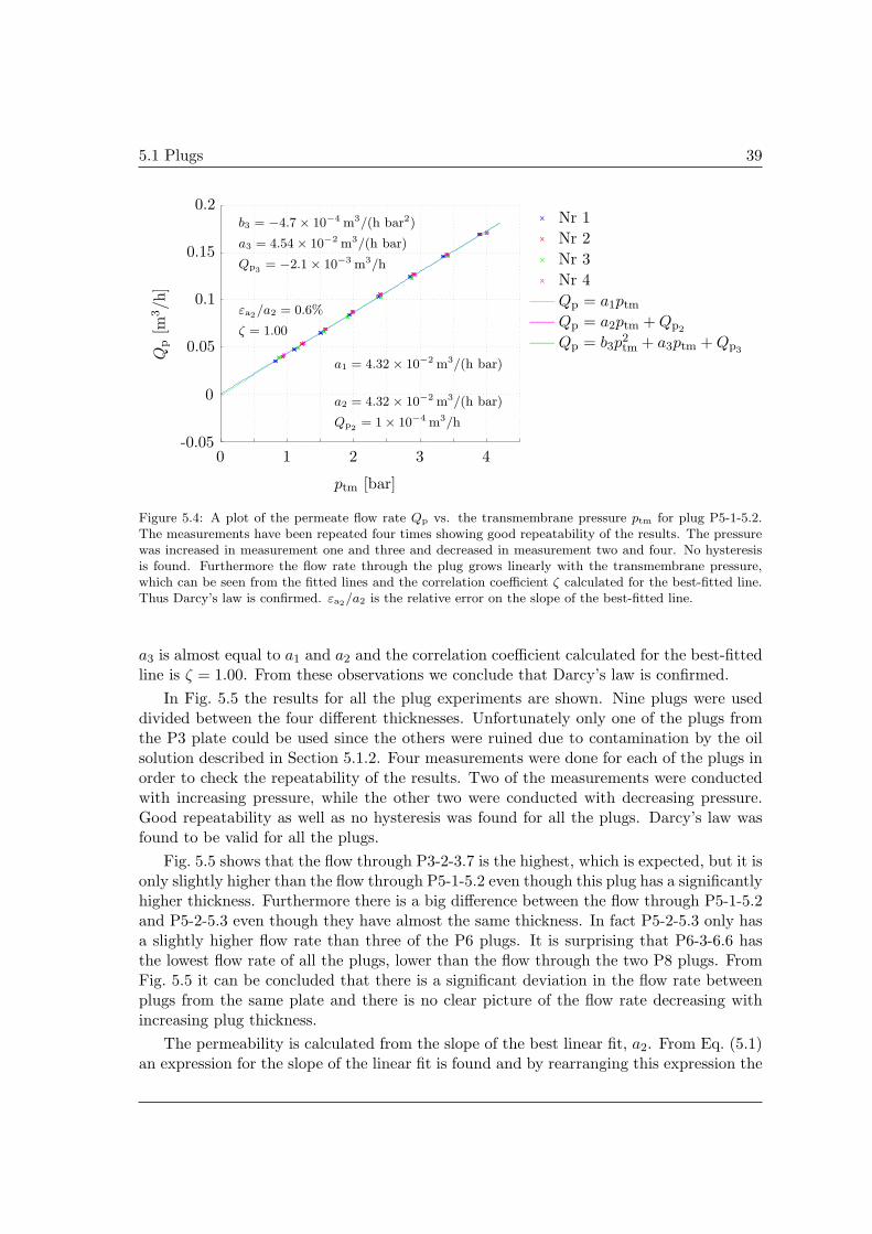
5.1 Plugs 39
-0.05
0
0.05
0.1
0.15
0.2
0 1 2 3 4
Qp
[m3/h
]
ptm [bar]
x Nr 1x Nr 2x Nr 3x Nr 4
Qp = a1ptm
Qp = a2ptm + Qp2
Qp = b3p2tm + a3ptm + Qp3
a1 = 4.32 × 10⁻² m3/(h bar)
a2 = 4.32 × 10⁻² m3/(h bar)
Qp2= 1 × 10⁻⁴ m3/h
b3 = −4.7 × 10⁻⁴ m3/(h bar2)
a3 = 4.54 × 10⁻² m3/(h bar)
Qp3= −2.1 × 10⁻³ m3/h
εa2/a2 = 0.6%
ζ = 1.00
Figure 5.4: A plot of the permeate flow rate Qp vs. the transmembrane pressure ptm for plug P5-1-5.2.The measurements have been repeated four times showing good repeatability of the results. The pressurewas increased in measurement one and three and decreased in measurement two and four. No hysteresisis found. Furthermore the flow rate through the plug grows linearly with the transmembrane pressure,which can be seen from the fitted lines and the correlation coefficient ζ calculated for the best-fitted line.Thus Darcy’s law is confirmed. εa2/a2 is the relative error on the slope of the best-fitted line.
a3 is almost equal to a1 and a2 and the correlation coefficient calculated for the best-fittedline is ζ = 1.00. From these observations we conclude that Darcy’s law is confirmed.
In Fig. 5.5 the results for all the plug experiments are shown. Nine plugs were useddivided between the four different thicknesses. Unfortunately only one of the plugs fromthe P3 plate could be used since the others were ruined due to contamination by the oilsolution described in Section 5.1.2. Four measurements were done for each of the plugs inorder to check the repeatability of the results. Two of the measurements were conductedwith increasing pressure, while the other two were conducted with decreasing pressure.Good repeatability as well as no hysteresis was found for all the plugs. Darcy’s law wasfound to be valid for all the plugs.
Fig. 5.5 shows that the flow through P3-2-3.7 is the highest, which is expected, but it isonly slightly higher than the flow through P5-1-5.2 even though this plug has a significantlyhigher thickness. Furthermore there is a big difference between the flow through P5-1-5.2and P5-2-5.3 even though they have almost the same thickness. In fact P5-2-5.3 only hasa slightly higher flow rate than three of the P6 plugs. It is surprising that P6-3-6.6 hasthe lowest flow rate of all the plugs, lower than the flow through the two P8 plugs. FromFig. 5.5 it can be concluded that there is a significant deviation in the flow rate betweenplugs from the same plate and there is no clear picture of the flow rate decreasing withincreasing plug thickness.
The permeability is calculated from the slope of the best linear fit, a2. From Eq. (5.1)an expression for the slope of the linear fit is found and by rearranging this expression the
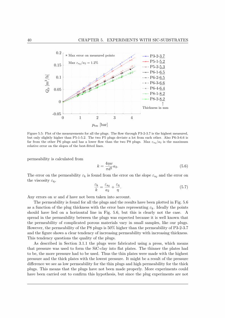
40 CHAPTER 5. EXPERIMENTS WITH SIC-SUBSTRATES
-0.05
0
0.05
0.1
0.15
0.2
0 1 2 3 4
Qp
[m3/h
]
ptm [bar]
x P3-2-3.7x P5-1-5.2x P5-2-5.3x P6-1-6.5x P6-2-6.5x P6-3-6.6x P6-4-6.4x P8-1-8.2x P8-2-8.2
Thickness in mm↑
Max error on measured points
Max εa2/a2 = 1.2%
Figure 5.5: Plot of the measurements for all the plugs. The flow through P3-2-3.7 is the highest measured,but only slightly higher than P5-1-5.2. The two P5 plugs deviate a lot from each other. Also P6-3-6.6 isfar from the other P6 plugs and has a lower flow than the two P8 plugs. Max εa2/a2 is the maximumrelative error on the slopes of the best-fitted lines.
permeability is calculated from
k =4ηw
πd2a2. (5.6)
The error on the permeability εk is found from the error on the slope εa2 and the error onthe viscosity εη,
εk
k=
εa2
a2+
εη
η. (5.7)
Any errors on w and d have not been taken into account.The permeability is found for all the plugs and the results have been plotted in Fig. 5.6
as a function of the plug thickness with the error bars representing εk. Ideally the pointsshould have lied on a horizontal line in Fig. 5.6, but this is clearly not the case. Aspread in the permeability between the plugs was expected because it is well known thatthe permeability of complicated porous materials vary in small samples, like our plugs.However, the permeability of the P8 plugs is 50% higher than the permeability of P3-2-3.7and the figure shows a clear tendency of increasing permeability with increasing thickness.This tendency questions the quality of the plugs.
As described in Section 3.1.1 the plugs were fabricated using a press, which meansthat pressure was used to form the SiC-clay into flat plates. The thinner the plates hadto be, the more pressure had to be used. Thus the thin plates were made with the highestpressure and the thick plates with the lowest pressure. It might be a result of the pressuredifference we see as low permeability for the thin plugs and high permeability for the thickplugs. This means that the plugs have not been made properly. More experiments couldhave been carried out to confirm this hypothesis, but since the plug experiments are not
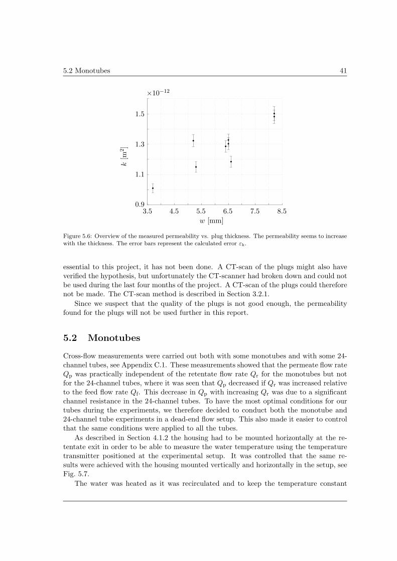
5.2 Monotubes 41
0.9
1.1
1.3
1.5
×10−12
3.5 4.5 5.5 6.5 7.5 8.5
k[m
2]
w [mm]
Figure 5.6: Overview of the measured permeability vs. plug thickness. The permeability seems to increasewith the thickness. The error bars represent the calculated error εk.
essential to this project, it has not been done. A CT-scan of the plugs might also haveverified the hypothesis, but unfortunately the CT-scanner had broken down and could notbe used during the last four months of the project. A CT-scan of the plugs could thereforenot be made. The CT-scan method is described in Section 3.2.1.
Since we suspect that the quality of the plugs is not good enough, the permeabilityfound for the plugs will not be used further in this report.
5.2 Monotubes
Cross-flow measurements were carried out both with some monotubes and with some 24-channel tubes, see Appendix C.1. These measurements showed that the permeate flow rateQp was practically independent of the retentate flow rate Qr for the monotubes but notfor the 24-channel tubes, where it was seen that Qp decreased if Qr was increased relativeto the feed flow rate Qf. This decrease in Qp with increasing Qr was due to a significantchannel resistance in the 24-channel tubes. To have the most optimal conditions for ourtubes during the experiments, we therefore decided to conduct both the monotube and24-channel tube experiments in a dead-end flow setup. This also made it easier to controlthat the same conditions were applied to all the tubes.
As described in Section 4.1.2 the housing had to be mounted horizontally at the re-tentate exit in order to be able to measure the water temperature using the temperaturetransmitter positioned at the experimental setup. It was controlled that the same re-sults were achieved with the housing mounted vertically and horizontally in the setup, seeFig. 5.7.
The water was heated as it was recirculated and to keep the temperature constant

42 CHAPTER 5. EXPERIMENTS WITH SIC-SUBSTRATES
(a)
0
1
2
3
4
0 0.4 0.8 1.2 1.6
Qp
[m3/h
]
ptm [bar]
x v., 20Cx h., 20Cx h., 20C*x h., 25C a2 Qp
2
[m3/(h bar)] [m3/h]
v., 20C 2.27 2.0× 10⁻³
h., 20C 2.24 1.4× 10⁻²
h., 20C* 2.25 1.1× 10⁻²
h., 25C 2.51 1.2× 10⁻²
(b)
εa2/a2 = 1.2%
Figure 5.7: (a) Control measurements of the experimental method with TI-XII-III. The housing waspositioned both vertically (’v.’) and horizontally (’h.’) and measurements were conducted at a watertemperature of 20C and 25C. The flow rate at 25C was compared to 20C (’20C*’), by compensatingthe difference in the viscosity of the water. No deviations were found. εa2/a2 is the relative error on theslope of the best-fitted lines, and it is representative for all the lines. (b) Table containing the constantsfor the best-fitted lines on the form Qp = a2ptm + Qp2 .
within ±0.5C, cold water had to be added to the water reservoir. It was very difficult tokeep the water at a temperature of 20C, and we therefore decided to run the experimentsat a water temperature of 25C. It was checked that changing the temperature did notchange the results, see Fig. 5.7. The flow rate measured at 25C was higher due to thelower viscosity of the water. When compensating the flow rate at 25C by the change inviscosity from 20C to 25C, using table A.8 in [3], the same flow rate as measured at20C was achieved.
During all the tube experiments (both monotubes and 24-channel tubes) a water tem-perature of approximately 25 ± 0.5C is used. In all the results presented in this thesisthe measured flow rate has been compensated to 20C using the average temperaturemeasured in each of the experiments.
A 2D flow approximation can be used for the water flow in the substrate of the mono-tubes. Therefore Darcy’s law is used on the form given in Eq. (2.41) and repeated herefor convenience
Qp =2πLk
ηln(1 + 2w
dc
)ptm, (5.8)
where dc is the channel diameter of the monotube, L is the monotube length, w is thewall thickness and ptm = (pf + pr)/2 − pp is the transmembrane pressure, see Eq. (2.22),with pf, pr and pp being the feed, retentate and permeate pressures, respectively.
The error on the measured data is calculated in the same way as given in Section 5.1.1with only one difference. Since ptm is now found using three measured pressures, theerror has changed. All three pressure transmitters have a maximum error of 0.5% of their
5.2 Monotubes 43
full-scale value. Using the standard method the error on ptm can then be calculated to be
εptm =εpf
+ εpr
2+ εpp =
0.02 bar + 0.02 bar2
+ 0.008 bar = 0.028 bar. (5.9)
From [12] we know that the upper limit of Darcy flow is Re ≈ 2.3 where the Reynoldsnumber is based on the mean grain diameter. We can calculate an approximate value ofthe maximum permeate flow rate that should be used in the monotube experiments. Thevelocity v0 in the porous SiC is found from the Reynolds number as
v0 =2.3η
ρdm= 0.23 m/s (5.10)
using a SiC mean grain diameter of dm = 10 µm and water with ρ = 1000 kg/m3 andη = 10−3 Pa s. Hereafter the maximum flow rate Qmax is found by integrating v0 overthe channel surface area of the tubes, Qmax = v0πLdc. With L = 305 mm and dc,thin =16.9mm and dc,thick = 14.1mm for the thin and thick-walled monotubes, respectively, theflow rates are
Qmax,thin ≈ 13.4m3/h, (5.11)
Qmax,thick ≈ 11.2m3/h, (5.12)
where Qmax,thin and Qmax,thick are the maximum allowed permeate flow rate through athin-walled and thick-walled monotube, respectively. As Qmax,thin and Qmax,thick are bothvery high the flow in the SiC should not exceed Darcy flow in our monotube experiments.
5.2.1 Short thin-walled monotubes
The repeatability of the tube experiments was checked in the same way as with the plugexperiments and it was also checked frequently if the tubes got contaminated. In Fig. 5.8four measurements, each with eight measuring points, have been conducted with mono-tube TI-XII-II. The pressure was increased in measurement one and three and decreasedin measurement two and four. No hysteresis was found and the measurements show goodrepeatability of the experiments. PT01 and PT02, measuring the feed and retentate pres-sure, respectively, showed an insignificant pressure drop down the length of the monotubein the order of 10−2 bar at the highest flow rates, thus the channel resistance in the mono-tube is negligible.
Three lines have been fitted to the data, a linear fit through (0, 0) (cyan line), a bestlinear fit (magenta) and a power-law fit (green) on the form Qp = Qp3
(ptm/1 bar)c3 . Thisform is used because when the fit is linear c3 = 1, but if the resistance in the monotubechannel becomes significant the Qp-ptm relation becomes nonlinear and c3 < 1. FromSection 2.3 it is known that in fully turbulent channel flow the relation is Q ∼ p4/7, andthus it is expected that 4/7 < c3 < 1, if a nonlinear relation is seen.
From the three fitted lines it is clear, that there is a linear relation between Qp and ptm
going through (0, 0). a1 and a2 are identical within the error on a2 which was calculated tobe εa2 = 3.2× 10⁻² m3/(h bar) and Qp2
is zero within the error of εQp2= 2.6× 10⁻² m3/h

44 CHAPTER 5. EXPERIMENTS WITH SIC-SUBSTRATES
0
1
2
3
4
0 0.4 0.8 1.2 1.6
Qp
[m3/h
]
ptm [bar]
x Nr 1x Nr 2x Nr 3x Nr 4
Qp = a1ptm
Qp = a2ptm + Qp2
Qp = Qp3
(
ptm
1 bar
)
c3
a1 = 2.60 m3/(h bar)
a2 = 2.58 m3/(h bar)
Qp2= 2.2 × 10⁻² m3/h
c3 = 1.0
Qp3= 2.61 m3/h
εa2/a2 = 1.2%
ζ = 1.00
Figure 5.8: A plot of the permeate flow rate Qp vs. the transmembrane pressure ptm for monotube TI-XII-II. The measurements have been repeated four times showing good repeatability of the results. Thepressure was increased in measurement one and three and decreased in measurement two and four. Nohysteresis is found. Furthermore, Qp grows linearly with ptm, which can be seen from the fitted lines andthe correlation coefficient ζ for the best-fitted line. Thus Darcy’s law is confirmed. εa2/a2 is the relativeerror on the slope of the best-fitted line.
as well. Furthermore c3 = 1.0 in the power-law fit and the correlation coefficient ζ = 1.00for the best-fitted line, which also confirms the linear relation.
In Fig. 5.9 all the measured data for the nine thin-walled monotube substrates used inthe experiments are shown. The lines are the best-fitted linear lines. Four measurements,each with eight measuring points, were done for each of the nine monotubes, all of themshowing good repeatability. Darcy’s law was found to be applicable for all the tubes. Theaverage constants including the standard deviation from each of the best-fitted lines are,as = (2.6 ± 0.2)m3/(h bar) and Qps
= (0.05 ± 0.02)m3/h, where subscript ’s’ stands forsubstrate.
A spread of 30% is found on the slope of the best-fitted lines which can be directlytransferred to a spread in the permeability of the tubes. As mentioned a spread of thissize is not surprising due to a dispersion in the permeability of relatively small samplesof porous materials. Furthermore the extrusion pressure in our fabrication method wasdifficult to control and different extrusion pressures might have led to a dispersion in thepermeability. Fabrication of the monotubes is described in Section 3.1.2. As for the plugsthe permeability of the monotubes is calculated from the slope of the best linear fit, a2,where an expression for a2 is found from Eq. (5.8). By rearranging this expression thepermeability is calculated from
k =ηln
(1 + 2w
dc
)
2πLa2. (5.13)
Using Eq. (5.13) the permeability is found for all the monotubes and the mean permeability

5.2 Monotubes 45
0
2
4
6
0 0.4 0.8 1.2 1.6 2
Qp
[m3/h
]
ptm [bar]
x TI-VI-Ix TI-VI-IIx TI-VI-IIIx TI-X-Ix TI-X-IIx TI-XII-Ix TI-XII-IIx TI-XII-IIIx TI-XVII-II
Max error on measured points
Max εa2/a2 = 1.3%
Figure 5.9: Plot of the measurements for all the thin-walled monotubes used. The spread on the slope ofthe best-fitted lines is 30%. The average slope as and average intersection Qps with the Qp-axis plus theirstandard deviations from the best linear fits are, as = (2.6± 0.2)m3/(h bar) and Qps = (0.05± 0.02)m3/h.Max εa2/a2 is the maximum relative error on the slopes of the best-fitted lines.
is then found to bekm,thin = (8.6± 0.8)× 10−13 m2, (5.14)
where the error is the standard deviation of the permeability from each of the monotubes.The error on the slope on the best-fitted lines from each of the monotubes is not takeninto account as it is negligible compared to the spread between the monotubes.
5.2.2 Thick-walled monotubes
The experiments with the thick-walled monotubes showed the same tendencies as theexperiments with the thin-walled monotubes. Seven of the thick-walled monotubes wereused and the measured data is shown in Fig. 5.10. Again four measurements, each witheight measuring points, were done for each of the monotubes and good repeatability wasfound. As for the thin-walled monotubes, Darcy’s law was found to be valid in theseexperiments as well. The average constants including the standard deviation from each ofthe best-fitted lines are, as = (1.29± 0.09)m3/(h bar) and Qps
= (0.06± 0.02)m3/h.Fig. 5.10 shows a spread in the flow rate between the monotubes as was also the case
with the thin-walled monotubes. The spread on the slope of the best-fitted lines is 20%.The permeability of the tubes is calculated using Eq. (5.13) and the mean value is
km,thick = (7.9± 0.5)× 10−13 m2, (5.15)
where the error is the standard deviation of the permeability from each of the monotubes.This permeability is a bit lower than the mean permeability found for the thin-walledtubes, see Eq. (5.14). Taking the error on the permeability into account, the permeabilities
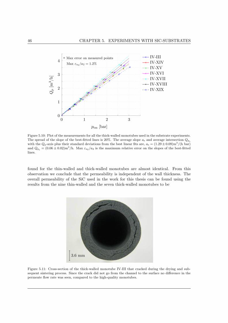
46 CHAPTER 5. EXPERIMENTS WITH SIC-SUBSTRATES
0
1
2
3
4
0 1 2 3
Qp
[m3/h
]
ptm [bar]
x IV-IIIx IV-XIVx IV-XVx IV-XVIx IV-XVIIx IV-XVIIIx IV-XIX
Max error on measured points
Max εa2/a2 = 1.2%
Figure 5.10: Plot of the measurements for all the thick-walled monotubes used in the substrate experiments.The spread of the slope of the best-fitted lines is 20%. The average slope as and average intersection Qps
with the Qp-axis plus their standard deviations from the best linear fits are, as = (1.29± 0.09)m3/(h bar)and Qps = (0.06 ± 0.02)m3/h. Max εa2/a2 is the maximum relative error on the slopes of the best-fittedlines.
found for the thin-walled and thick-walled monotubes are almost identical. From thisobservation we conclude that the permeability is independent of the wall thickness. Theoverall permeability of the SiC used in the work for this thesis can be found using theresults from the nine thin-walled and the seven thick-walled monotubes to be
3.6 mm
Figure 5.11: Cross-section of the thick-walled monotube IV-III that cracked during the drying and sub-sequent sintering process. Since the crack did not go from the channel to the surface no difference in thepermeate flow rate was seen, compared to the high-quality monotubes.
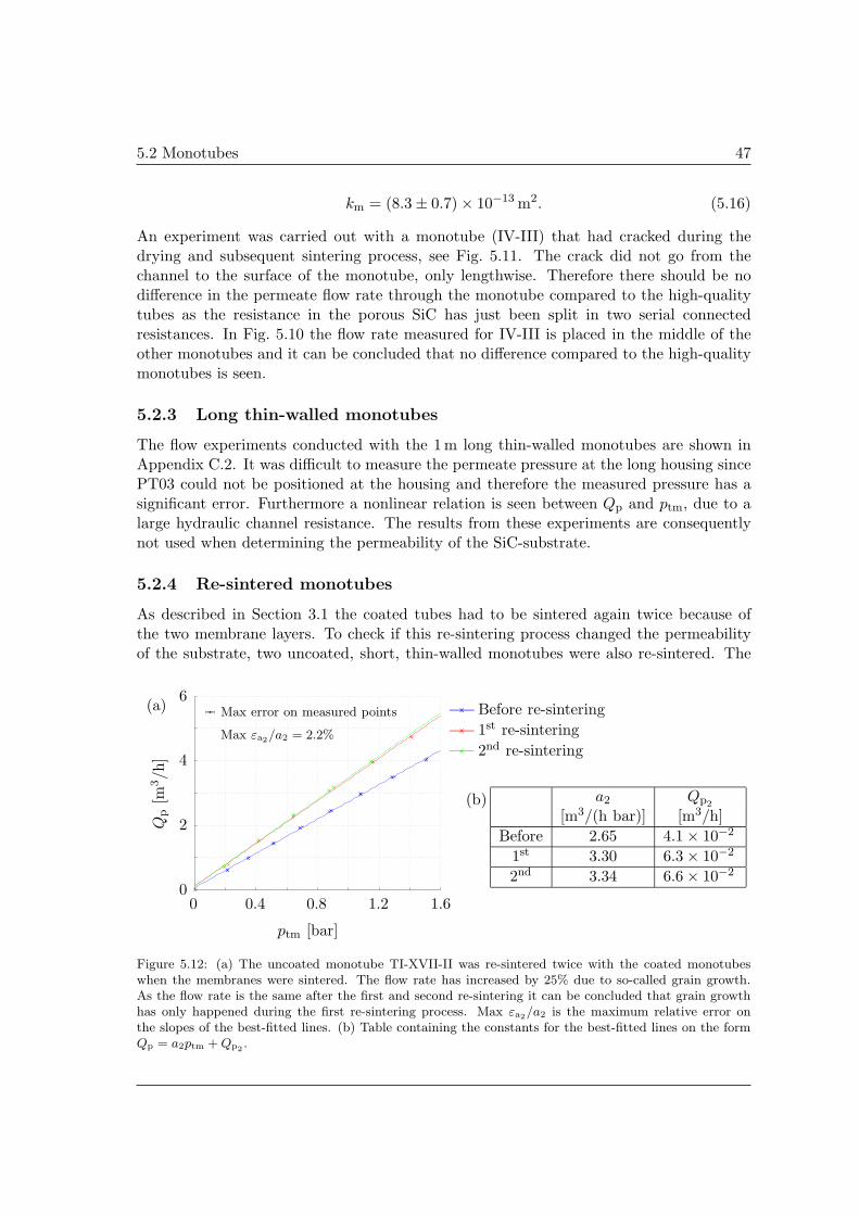
5.2 Monotubes 47
km = (8.3± 0.7)× 10−13 m2. (5.16)
An experiment was carried out with a monotube (IV-III) that had cracked during thedrying and subsequent sintering process, see Fig. 5.11. The crack did not go from thechannel to the surface of the monotube, only lengthwise. Therefore there should be nodifference in the permeate flow rate through the monotube compared to the high-qualitytubes as the resistance in the porous SiC has just been split in two serial connectedresistances. In Fig. 5.10 the flow rate measured for IV-III is placed in the middle of theother monotubes and it can be concluded that no difference compared to the high-qualitymonotubes is seen.
5.2.3 Long thin-walled monotubes
The flow experiments conducted with the 1 m long thin-walled monotubes are shown inAppendix C.2. It was difficult to measure the permeate pressure at the long housing sincePT03 could not be positioned at the housing and therefore the measured pressure has asignificant error. Furthermore a nonlinear relation is seen between Qp and ptm, due to alarge hydraulic channel resistance. The results from these experiments are consequentlynot used when determining the permeability of the SiC-substrate.
5.2.4 Re-sintered monotubes
As described in Section 3.1 the coated tubes had to be sintered again twice because ofthe two membrane layers. To check if this re-sintering process changed the permeabilityof the substrate, two uncoated, short, thin-walled monotubes were also re-sintered. The
(a)
0
2
4
6
0 0.4 0.8 1.2 1.6
Qp
[m3/h
]
ptm [bar]
x Before re-sinteringx 1st re-sinteringx 2nd re-sintering
a2 Qp2
[m3/(h bar)] [m3/h]
Before 2.65 4.1× 10⁻²
1st 3.30 6.3× 10⁻²
2nd 3.34 6.6× 10⁻²
(b)
Max error on measured points
Max εa2/a2 = 2.2%
Figure 5.12: (a) The uncoated monotube TI-XVII-II was re-sintered twice with the coated monotubeswhen the membranes were sintered. The flow rate has increased by 25% due to so-called grain growth.As the flow rate is the same after the first and second re-sintering it can be concluded that grain growthhas only happened during the first re-sintering process. Max εa2/a2 is the maximum relative error onthe slopes of the best-fitted lines. (b) Table containing the constants for the best-fitted lines on the formQp = a2ptm + Qp2 .

48 CHAPTER 5. EXPERIMENTS WITH SIC-SUBSTRATES
measurements conducted with TI-XVII-II are shown in Fig. 5.12. The figure shows asignificant increase of 25% in the flow rate after the first re-sintering, while there is nochange from the first to the second re-sintering. The same was seen for the other re-sinteredmonotube, TI-VI-III.
This increase in the flow rate is due to a so-called grain growth in the SiC, which meansthat the SiC-grains in the substrate increase their size, [22]. During the re-sintering theinternal energy can only be reduced by decreasing the grain boundary area, thus smallgrains are consumed by larger grains and sharp edges become more round. Such a graingrowth results in larger pores in the SiC-substrate and therefore a higher permeability.Since there is no change in the flow rate from the first to the second re-sintering it can beseen that the grain growth only occurs during the first re-sintering process.
Only two monotubes were re-sintered and therefore we cannot conclude that the per-meability changes in the substrate during the re-sintering, but only state that there is aclear tendency that this is the case. In order to give a more significant conclusion, moremonotubes should have been re-sintered.
5.3 24-channel tubes
The experiments with the 24-channel tubes were conducted in a dead-end flow setup inthe same way as the monotube experiments. The 24-channel tubes are not used in orderto find the permeability of the SiC-material, but in order to introduce a more complexgeometry in the thesis which is used by CoMeTas in some of their membranes.
In Fig. 5.13 four measurements carried out for XXIV-V are shown. As with the mono-
0
2
4
6
0 0.2 0.4 0.6 0.8 1
Qp
[m3/h
]
ptm [bar]
x Nr 1x Nr 2x Nr 3x Nr 4
Qp = a1ptm
Qp = a2ptm + Qp2
Qp = Qp3
(
ptm
1 bar
)
c3
· Error on power-law fita1 = 5.38 m3/(h bar)
a2 = 4.68 m3/(h bar)
Qp2= 0.42 m3/h
c3 = 0.82
Qp3= 5.01 m3/h
Figure 5.13: A plot of the permeate flow rate Qp vs. the transmembrane pressure ptm for 24-channeltube XXIV-V. The flow rate is not linearly related to the transmembrane pressure because the channelresistance in the tube becomes significant.
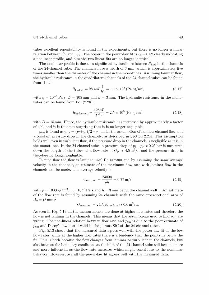
5.3 24-channel tubes 49
tubes excellent repeatability is found in the experiments, but there is no longer a linearrelation between Qp and ptm. The power in the power-law fit is c3 = 0.82 clearly indicatinga nonlinear profile, and also the two linear fits are no longer identical.
The nonlinear profile is due to a significant hydraulic resistance Rhyd in the channelsof the 24-channel tube. The channels have a width of 3 mm, which is approximately fivetimes smaller than the diameter of the channel in the monotubes. Assuming laminar flow,the hydraulic resistance in the quadrilateral channels of the 24-channel tubes can be foundfrom [1] as
Rhyd,24 = 28.4ηL1h4
= 1.1× 10⁸ (Pa s)/m3, (5.17)
with η = 10−3 Pa s, L = 305 mm and h = 3mm. The hydraulic resistance in the mono-tubes can be found from Eq. (2.28),
Rhyd,mono =128ηL
D4π= 2.5× 10⁵ (Pa s)/m3, (5.18)
with D = 15 mm. Hence, the hydraulic resistance has increased by approximately a factorof 400, and it is thus not surprising that it is no longer negligible.
ptm is found as ptm = (pf+pr)/2−pp under the assumption of laminar channel flow anda constant pressure drop in the channels, as described in Section 2.2.4. This assumptionholds well even in turbulent flow, if the pressure drop in the channels is negligible as it is inthe monotubes. In the 24-channel tubes a pressure drop of pf − pr ≈ 0.25 bar is measureddown the length of the tubes at a flow rate of Qp ≈ 4.5m3/h and the pressure drop istherefore no longer negligible.
In pipe flow the flow is laminar until Re ≈ 2300 and by assuming the same averagevelocity in the channels, an estimate of the maximum flow rate with laminar flow in thechannels can be made. The average velocity is
vmax,lam =2300η
ρh= 0.77m/s, (5.19)
with ρ = 1000 kg/m3, η = 10−3 Pa s and h = 3mm being the channel width. An estimateof the flow rate is found by assuming 24 channels with the same cross-sectional area ofAc = (3 mm)2
Qmax,lam = 24Acvmax,lam ≈ 0.6 m3/h. (5.20)
As seen in Fig. 5.13 all the measurements are done at higher flow rates and therefore theflow is not laminar in the channels. This means that the assumptions used to find ptm arewrong. The non-linear relation between flow rate and ptm is due to the poor estimate ofptm and Darcy’s law is still valid in the porous SiC of the 24-channel tubes.
Fig. 5.13 shows that the measured data agrees well with the power-law fit at the lowflow rates, while at the higher flow rates there is a tendency that the points lie below thefit. This is both because the flow changes from laminar to turbulent in the channels, butalso because the boundary conditions at the inlet of the 24-channel tube will become moreand more influential as the flow rate increases which might contribute to the nonlinearbehavior. However, overall the power-law fit agrees well with the measured data.

50 CHAPTER 5. EXPERIMENTS WITH SIC-SUBSTRATES
0
2
4
6
0 0.2 0.4 0.6 0.8 1
Qp
[m3/h
]
ptm [bar]
x XXIV-IIIx XXIV-IVx XXIV-Vx XXIV-VIx XXIV-VIIx XXIV-Xx XXIV-XI
Max error on measured points
· Error on power-law fit
Figure 5.14: Plot of the measurements for all the 24-channel tubes used in the substrate experiments.The error of the fitted lines is shown in three places on the slope of XXIV-XI. The error bars in thisfigure are representative for all the measurements for the 24-channel tubes. The spread in the flow rateis approximately 20%. The mean constants including their standard deviations found from the power-lawfits are, cs = 0.82± 0.02 and Qps = (5.3± 0.3)m3/h.
The error on the measured data is found in the same way as for the monotubes with onlya few differences. Since the flow rate is no longer linearly related to the transmembranepressure, the error on the measured flow rate is found relative to the power-law fit insteadof the best linear fit. Also, the error is no longer calculated for the best-fitted linear linebut instead for the power-law fit. This is done by fitting two lines to the measured pointswith their error added and subtracted, respectively, and using these two lines as a measureof the error on the power-law fit.
Fig. 5.14 shows all the data for the seven 24-channel tubes used in the substrateexperiments. Just like for the monotubes a spread is seen in the flow rate between thetubes, which is approximately 20%. The 24-channel tubes were fabricated by LiqTech incontrolled conditions, as described in Section 3.1.3, and since the tubes have a dispersionin the flow rate (and thus also in the permeability) of the same size as found for themonotubes, it confirms that we have fabricated monotubes of high quality.
All the 24-channel tubes have a nonlinear Qp-ptm relation and follows the power-lawfit very well. It is consistent for all the tubes that the highest measured flow rates lieslightly below the fitted lines which is most likely due to the reasons described above.
5.4 Summary
Experiments with the plugs and monotubes confirm Darcy’s linear law for flow in porousmaterials. Furthermore, all experiments show good repeatability of the results and theerror on the experimental method is low.

5.4 Summary 51
Table 5.1: The measured permeabilities k, in m2, from the experiments with the thin-walled and thethick-walled monotubes plus the overall permeability from both experiments. It is concluded that thepermeability is independent of the thickness. The errors are the standard deviations of the permeabilityfound from each of the used monotubes.
k [m2]Thin-walled (8.6± 0.8)× 10−13
Thick-walled (7.9± 0.5)× 10−13
Overall (8.3± 0.7)× 10−13
In the plug experiments nine plugs divided between four different thicknesses are usedand the results show a clear tendency of increasing permeability with increasing thickness.Due to this tendency it is concluded that the plugs have not been fabricated properly andthe permeabilities calculated from these experiments are therefore rejected.
During plug experiments several problems concerning the experimental method aresolved and much experience is achieved with the experimental setup and method whichproved valuable when tube experiments were carried out.
Monotube experiments show good agreement for the permeability found from the ninethin-walled and seven thick-walled monotubes and we conclude that the permeability isindependent of the wall thickness. The permeabilities are given in Table 5.1. A dispersionof up to 30% is measured in flow rate between the tubes and this tendency is seen for bothmonotubes and 24-channel tubes. It is expected that this dispersion is due to a variationin the permeability in between the tubes since the tubes are relatively small SiC-samples.
Experiments with 24-channel tubes show that the Qp-ptm relation no longer is linear.This nonlinearity is because of the hydraulic resistance in the channels of the tube beingsignificant leading to a high pressure drop down the length of the 24-channel tubes. As thechannel flow is not laminar the pressure drop is nonlinear in the channels. The estimateof the transmembrane pressure is therefore poor, which is the reason for the nonlinearrelation between Qp and ptm. Darcy’s law is still valid in the porous SiC of the 24-channeltubes.

52 CHAPTER 5. EXPERIMENTS WITH SIC-SUBSTRATES
Chapter 6
Experiments with coatedSiC-tubes
An essential part of the filters used by CoMeTas is the membrane layer added to the surfaceof the channels. We therefore coated some of our thin-walled monotubes and some of our24-channel tubes with two membrane layers as described in Section 3.1.4. All the tubeswere coated with the same middle layer using a 1µm membrane, while two different typesof membrane were used for the outer layer, a 0.1µm membrane and a 0.04µm membrane.These membranes were chosen because CoMeTas uses them in their filters. Since the0.04 µm membrane is the one most often used by CoMeTas, most of the tubes were coatedwith this membrane.
In the following we describe the experiments conducted with the coated monotubes and24-channel tubes. We first present our experiments with the monotubes, which are usedto find an estimate of the permeability in the two outer membrane layers. This membranepermeability can later be used in our simulations. Second we present our experimentswith the 24-channel tubes, which will be used to verify our numerical models, just like the24-channel tube substrate experiments.
In Chapter 5 we found that the error on the experimental method was very low. Inorder to save time we have therefore only conducted two measurements, instead of four,with each of the coated tubes in this chapter.
We have investigated the thickness of the membrane layers and the quality of thecoating method by taking pictures of the membranes using a microscope. These picturesare also presented here.
6.1 Thin-walled monotubes
Some initial experiments were conducted with four monotubes after they had been coatedwith the 1µm membrane. These experiments were carried out in order to see how thismembrane affected the permeate flow rate through the tubes and they are presented inAppendix C.3.1. As expected the flow rate was still linearly related to the transmembranepressure and a minor decrease in the flow rate of approximately 15% was found when
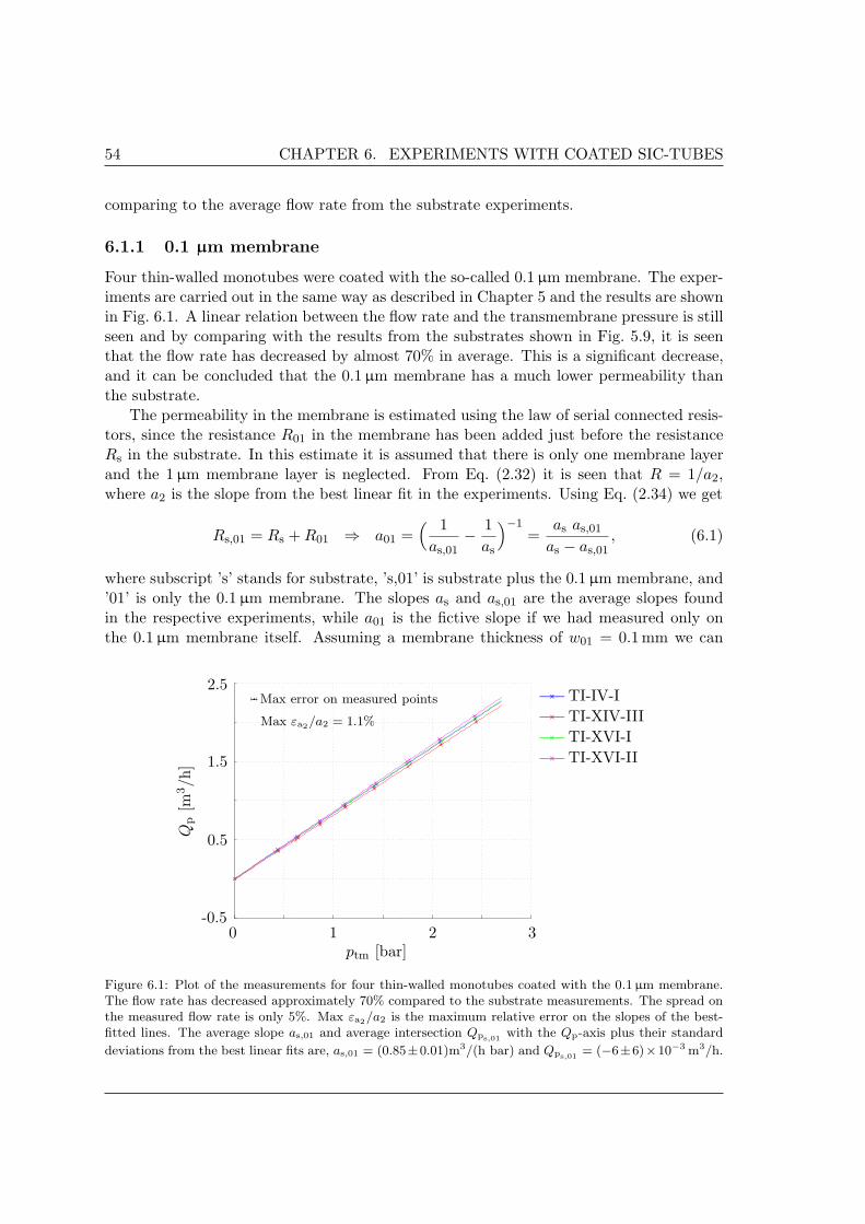
54 CHAPTER 6. EXPERIMENTS WITH COATED SIC-TUBES
comparing to the average flow rate from the substrate experiments.
6.1.1 0.1 µm membrane
Four thin-walled monotubes were coated with the so-called 0.1 µm membrane. The exper-iments are carried out in the same way as described in Chapter 5 and the results are shownin Fig. 6.1. A linear relation between the flow rate and the transmembrane pressure is stillseen and by comparing with the results from the substrates shown in Fig. 5.9, it is seenthat the flow rate has decreased by almost 70% in average. This is a significant decrease,and it can be concluded that the 0.1µm membrane has a much lower permeability thanthe substrate.
The permeability in the membrane is estimated using the law of serial connected resis-tors, since the resistance R01 in the membrane has been added just before the resistanceRs in the substrate. In this estimate it is assumed that there is only one membrane layerand the 1µm membrane layer is neglected. From Eq. (2.32) it is seen that R = 1/a2,where a2 is the slope from the best linear fit in the experiments. Using Eq. (2.34) we get
Rs,01 = Rs + R01 ⇒ a01 =( 1
as,01− 1
as
)−1=
as as,01
as − as,01, (6.1)
where subscript ’s’ stands for substrate, ’s,01’ is substrate plus the 0.1 µm membrane, and’01’ is only the 0.1µm membrane. The slopes as and as,01 are the average slopes foundin the respective experiments, while a01 is the fictive slope if we had measured only onthe 0.1µm membrane itself. Assuming a membrane thickness of w01 = 0.1mm we can
-0.5
0.5
1.5
2.5
0 1 2 3
Qp
[m3/h
]
ptm [bar]
x TI-IV-Ix TI-XIV-IIIx TI-XVI-Ix TI-XVI-II
Max error on measured points
Max εa2/a2 = 1.1%
Figure 6.1: Plot of the measurements for four thin-walled monotubes coated with the 0.1 µm membrane.The flow rate has decreased approximately 70% compared to the substrate measurements. The spread onthe measured flow rate is only 5%. Max εa2/a2 is the maximum relative error on the slopes of the best-fitted lines. The average slope as,01 and average intersection Qps,01 with the Qp-axis plus their standard
deviations from the best linear fits are, as,01 = (0.85±0.01)m3/(h bar) and Qps,01 = (−6±6)×10−3 m3/h.
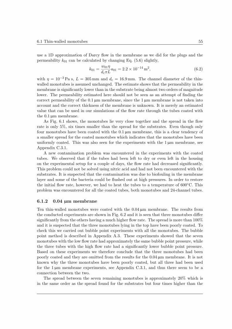
6.1 Thin-walled monotubes 55
use a 1D approximation of Darcy flow in the membrane as we did for the plugs and thepermeability k01 can be calculated by changing Eq. (5.6) slightly,
k01 =w01η
dcπLa01 = 2.2× 10⁻¹⁴ m2, (6.2)
with η = 10−3 Pa s, L = 305 mm and dc = 16.9mm. The channel diameter of the thin-walled monotubes is assumed unchanged. The estimate shows that the permeability in themembrane is significantly lower than in the substrate being almost two orders of magnitudelower. The permeability estimated here should not be seen as an attempt of finding thecorrect permeability of the 0.1µm membrane, since the 1µm membrane is not taken intoaccount and the correct thickness of the membrane is unknown. It is merely an estimatedvalue that can be used in our simulations of the flow rate through the tubes coated withthe 0.1µm membrane.
As Fig. 6.1 shows, the monotubes lie very close together and the spread in the flowrate is only 5%, six times smaller than the spread for the substrates. Even though onlyfour monotubes have been coated with the 0.1µm membrane, this is a clear tendency ofa smaller spread for the coated monotubes which indicates that the monotubes have beenuniformly coated. This was also seen for the experiments with the 1µm membrane, seeAppendix C.3.1.
A new contamination problem was encountered in the experiments with the coatedtubes. We observed that if the tubes had been left to dry or even left in the housingon the experimental setup for a couple of days, the flow rate had decreased significantly.This problem could not be solved using nitric acid and had not been encountered with thesubstrates. It is suspected that the contamination was due to biofouling in the membranelayer and some of the bacteria could be flushed out at high pressures. In order to restorethe initial flow rate, however, we had to heat the tubes to a temperature of 600C. Thisproblem was encountered for all the coated tubes, both monotubes and 24-channel tubes.
6.1.2 0.04 µm membrane
Ten thin-walled monotubes were coated with the 0.04µm membrane. The results fromthe conducted experiments are shown in Fig. 6.2 and it is seen that three monotubes differsignificantly from the others having a much higher flow rate. The spread is more than 100%and it is suspected that the three monotubes lying in the top have been poorly coated. Tocheck this we carried out bubble point experiments with all the monotubes. The bubblepoint method is described in Appendix A.3. These experiments showed that the sevenmonotubes with the low flow rate had approximately the same bubble point pressure, whilethe three tubes with the high flow rate had a significantly lower bubble point pressure.Based on these experiments we therefore conclude that the three monotubes had beenpoorly coated and they are omitted from the results for the 0.04 µm membrane. It is notknown why the three monotubes have been poorly coated, but all three had been usedfor the 1µm membrane experiments, see Appendix C.3.1, and thus there seem to be aconnection between the two.
The spread between the seven remaining monotubes is approximately 20% which isin the same order as the spread found for the substrates but four times higher than the

56 CHAPTER 6. EXPERIMENTS WITH COATED SIC-TUBES
-0.5
0.5
1.5
2.5
3.5
0 0.5 1 1.5 2 2.5
Qp
[m3/h
]
ptm [bar]
x TI-IV-IIx TI-X-IIx TI-XII-Ix TI-XIV-Ix TI-XIV-IIx TI-XVI-IIIx TI-XVIII-Ix TI-XX-Ix TI-XX-IIx TI-XX-III
Max error on measured points
Max εa2/a2 = 1.6%
Figure 6.2: Plot of the measurements for the ten thin-walled monotubes coated with the 0.04 µm membrane.Big variations of more than 100% are seen in the flow rate. Seven monotubes lie reasonably close in thebottom, while the three last monotubes differ significantly having a much higher flow rate due to poorcoating. The flow rate has decreased more than 70% for the monotubes in the bottom compared tothe substrate measurements. Max εa2/a2 is the maximum relative error on the slopes of the best-fittedlines. The mean slope as,004 and mean intersection with the Qp-axis Qps,004 plus their standard deviations
from the best linear fits of the seven monotubes in the bottom are, as,004 = (0.75 ± 0.05)m3/(h bar) andQps,004 = (−2± 4)× 10−3 m3/h.
spread found for the monotubes coated with the 0.1µm membrane. This indicates thatthe monotubes with the 0.04µm membrane have not been as uniformly coated as themonotubes with the 0.1µm membrane. The reason for this is unknown.
The flow rate has decreased slightly more than 70% in average compared to the sub-strate experiments and it is practically the same as measured for the tubes coated withthe 0.1µm membrane. Since the average pore size in the 0.04µm membrane should beapproximately 2.5 times smaller than in the 0.1µm membrane, it was expected that theflow rate in the tubes with the 0.04µm membrane was significantly lower, assuming thesame membrane thickness. As the flow rates are approximately the same, it indicates thatthe 0.1µm membrane is thicker than the 0.04 µm membrane.
An estimate of the permeability k004 in the 0.04µm membrane is found using the sameassumptions as for the 0.1µm membrane. The fictive slope a004 is found from Eq. (6.1)with as,01 replaced by as,004 and the permeability is then found from Eq. (6.2) with amembrane thickness of w004 = 0.1mm,
k004 = 1.8× 10⁻¹⁴ m2. (6.3)
6.1.3 Investigation of the membrane thickness
This section has been abridged, and only the most important tendencies seen are described.Since we had some discrepancies in the experiments with our coated monotubes, we decided
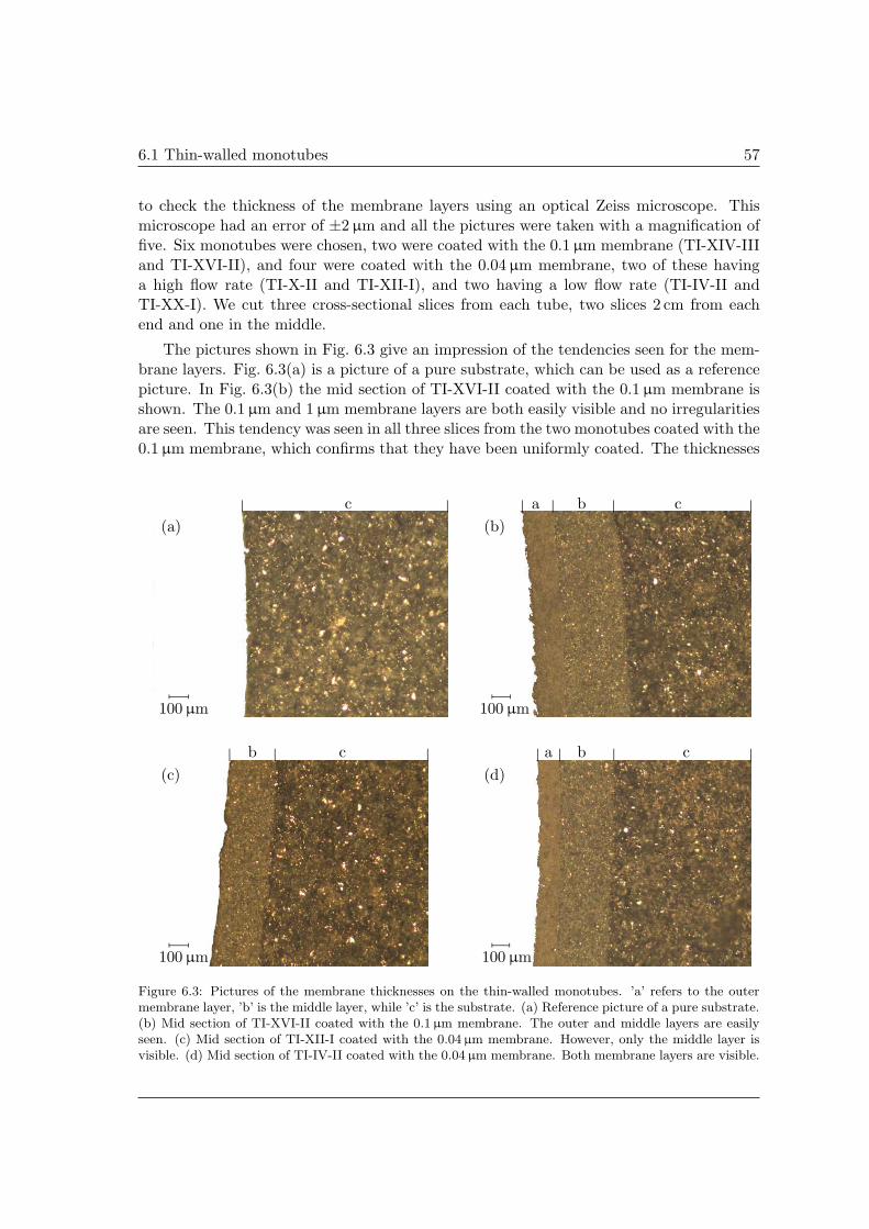
6.1 Thin-walled monotubes 57
to check the thickness of the membrane layers using an optical Zeiss microscope. Thismicroscope had an error of ±2µm and all the pictures were taken with a magnification offive. Six monotubes were chosen, two were coated with the 0.1µm membrane (TI-XIV-IIIand TI-XVI-II), and four were coated with the 0.04 µm membrane, two of these havinga high flow rate (TI-X-II and TI-XII-I), and two having a low flow rate (TI-IV-II andTI-XX-I). We cut three cross-sectional slices from each tube, two slices 2 cm from eachend and one in the middle.
The pictures shown in Fig. 6.3 give an impression of the tendencies seen for the mem-brane layers. Fig. 6.3(a) is a picture of a pure substrate, which can be used as a referencepicture. In Fig. 6.3(b) the mid section of TI-XVI-II coated with the 0.1µm membrane isshown. The 0.1 µm and 1µm membrane layers are both easily visible and no irregularitiesare seen. This tendency was seen in all three slices from the two monotubes coated with the0.1µm membrane, which confirms that they have been uniformly coated. The thicknesses
(a) (b)
(c) (d)
100 µm 100 µm
100 µm 100 µm
c a b c
b c a b c
Figure 6.3: Pictures of the membrane thicknesses on the thin-walled monotubes. ’a’ refers to the outermembrane layer, ’b’ is the middle layer, while ’c’ is the substrate. (a) Reference picture of a pure substrate.(b) Mid section of TI-XVI-II coated with the 0.1 µm membrane. The outer and middle layers are easilyseen. (c) Mid section of TI-XII-I coated with the 0.04 µm membrane. However, only the middle layer isvisible. (d) Mid section of TI-IV-II coated with the 0.04 µm membrane. Both membrane layers are visible.
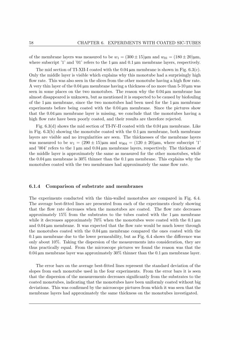
58 CHAPTER 6. EXPERIMENTS WITH COATED SIC-TUBES
of the membrane layers was measured to be w1 = (300± 15)µm and w01 = (180± 20)µm,where subscript ’1’ and ’01’ refers to the 1µm and 0.1µm membrane layers, respectively.
The mid section of TI-XII-I coated with the 0.04 µm membrane is shown in Fig. 6.3(c).Only the middle layer is visible which explains why this monotube had a surprisingly highflow rate. This was also seen in the slices from the other monotube having a high flow rate.A very thin layer of the 0.04µm membrane having a thickness of no more than 5-10µm wasseen in some places on the two monotubes. The reason why the 0.04µm membrane hasalmost disappeared is unknown, but as mentioned it is suspected to be caused by biofoulingof the 1 µm membrane, since the two monotubes had been used for the 1µm membraneexperiments before being coated with the 0.04µm membrane. Since the pictures showthat the 0.04µm membrane layer is missing, we conclude that the monotubes having ahigh flow rate have been poorly coated, and their results are therefore rejected.
Fig. 6.3(d) shows the mid section of TI-IV-II coated with the 0.04µm membrane. Likein Fig. 6.3(b) showing the monotube coated with the 0.1µm membrane, both membranelayers are visible and no irregularities are seen. The thicknesses of the membrane layerswas measured to be w1 = (290 ± 15)µm and w004 = (120 ± 20)µm, where subscript ’1’and ’004’ refers to the 1µm and 0.04 µm membrane layers, respectively. The thickness ofthe middle layer is approximately the same as measured for the other monotubes, whilethe 0.04µm membrane is 30% thinner than the 0.1µm membrane. This explains why themonotubes coated with the two membranes had approximately the same flow rate.
6.1.4 Comparison of substrate and membranes
The experiments conducted with the thin-walled monotubes are compared in Fig. 6.4.The average best-fitted lines are presented from each of the experiments clearly showingthat the flow rate decreases when the monotubes are coated. The flow rate decreasesapproximately 15% from the substrates to the tubes coated with the 1µm membranewhile it decreases approximately 70% when the monotubes were coated with the 0.1µmand 0.04µm membrane. It was expected that the flow rate would be much lower throughthe monotubes coated with the 0.04 µm membrane compared the ones coated with the0.1µm membrane due to the lower permeability, but as Fig. 6.4 shows the difference wasonly about 10%. Taking the dispersion of the measurements into consideration, they arethus practically equal. From the microscope pictures we found the reason was that the0.04 µm membrane layer was approximately 30% thinner than the 0.1µm membrane layer.
The error bars on the average best-fitted lines represent the standard deviation of theslopes from each monotube used in the four experiments. From the error bars it is seenthat the dispersion of the measurements decreases significantly from the substrates to thecoated monotubes, indicating that the monotubes have been uniformly coated without bigdeviations. This was confirmed by the microscope pictures from which it was seen that themembrane layers had approximately the same thickness on the monotubes investigated.

6.2 24-channel tubes 59
(a)
-1
1
3
5
0 0.5 1 1.5 2 2.5
Qp
[m3/h
]
ptm [bar]
x Substratex 1 µm membranex 0.1 µm membranex 0.04 µm membrane
a2 Qp2
[m3/(h bar)] [m3/h]
Sub. 2.6 ± 0.2 (5 ± 2) × 10−2
1 µm 2.12 ± 0.09 (3 ± 1) × 10−2
0.1 µm 0.85 ± 0.01 (−6 ± 6) × 10−3
0.04 µm 0.75 ± 0.05 (−2 ± 4) × 10−3
(b)
Figure 6.4: Comparison of thin-walled monotubes. (a) The mean best-fitted lines from the differentexperiments are plotted and the error bars represent the standard deviation of the slopes from the bestfits. (b) Table containing the average constants including their standard deviations for the best-fitted lineson the form Qp = a2ptm + Qp2 . The flow rate is almost equal for the 0.1 µm and the 0.04 µm membranedue to a higher thickness of the 0.1 µm membrane. The error decreases significantly from the substrate tothe membrane experiments, indicating that the monotubes have been uniformly coated.
6.2 24-channel tubes
As for the monotubes, initial experiments were conducted with four 24-channel tubescoated with the 1µm membrane, see Appendix C.3.2. The experiments showed a decreaseof 20% in average in the flow rate compared to the substrate experiments at ptm = 1bar,which is in the same magnitude as seen for the monotubes. Further, the experimentsshowed a spread of 25% in the flow rate between the tubes which is more than seen forthe monotubes. This might indicate that the 24-channel tubes have not been uniformlycoated with the 1µm membrane.
6.2.1 0.1 µm membrane
Four 24-channel tubes were coated with the 0.1µm membrane and the results from theexperiments are shown in Fig. 6.5. By comparing with the results from the substrateexperiments shown in Fig. 5.14, it is seen that the flow rate has decreased by approximately60% at a pressure of ptm = 1 bar. This is a bit less than the decrease seen for the monotubescoated with the 0.1µm membrane, which is partly because the Qp-ptm relation has becomemore linear for the coated 24-channel tubes due to the lower flow rate. The mean powerfor the tubes coated with the 0.1µm membrane is cs,01 = 0.93 , while it was cs = 0.83 forthe substrates clearly showing the more linear relation.
The spread in the flow rate is 12%, which is much lower than the spread seen in theexperiments with the four 24-channel tubes coated only with the 1µm membrane andalso lower than the spread found for the substrates. This decrease was also seen for themonotubes and again it indicates that the tubes have been uniformly coated.

60 CHAPTER 6. EXPERIMENTS WITH COATED SIC-TUBES
0
1
2
3
0 0.4 0.8 1.2
Qp
[m3/h
]
ptm [bar]
x XXIV-XVIIx XXIV-XVIIIx XXIV-XIXx XXIV-XX
Max error on measured points
· Error on power-law fit
Figure 6.5: Plot of the measurements for four 24-channel tubes coated with the 0.1 µm membrane. The flowrate has decreased approximately 60% compared to the substrate experiments and is almost linearly relatedto the transmembrane pressure. The error on the power-law fits is given in three places on the slope ofXXIV-XVIII. The spread on the measured flow rate from the tubes is 12%. The mean constants includingtheir standard deviations found from the power-law fits are, cs,01 = 0.93±0.01 and Qps,01 = (2.2±0.1)m3/h.
6.2.2 0.04 µm membrane
Eight 24-channel tubes were coated with the 0.04 µm membrane. The results from theexperiments are shown in Fig. 6.6 and it is seen that four of the 24-channel tubes lie veryclose in the bottom, while the other four differ significantly having a much higher flow rate.The exact same thing was seen for the monotubes coated with the 0.04µm membrane, andagain the four tubes with the high flow rate were the ones used for the 1µm membraneexperiments, see Appendix C.3.2. Bubble point experiments were carried out once moreand again a much lower bubble point pressure was measured for the four tubes having ahigh flow rate compared to the other tubes. Thus we conclude that these 24-channel tubeshave been poorly coated and they are omitted from the results for the 0.04 µm membrane.
Three of the four monotubes and all of the four 24-channel tubes used for the 1µmmembrane experiments have then been poorly coated with the second membrane layer.This has undoubtedly something to do with them being used in these experiments andit might be because of a biofouling layer, which prevents the 0.04µm membrane fromsticking to the surface of the tubes. This hypothesis has not been investigated, though,since it is not an important part of the work for this thesis.
The flow rate in the four 24-channel tubes lying in the bottom of Fig. 6.6 has decreasedapproximately 60% compared to the substrate experiments, and they have practically thesame flow rate as the 24-channel tubes coated with the 0.1µm membrane. Qp and ptm
are almost linearly related with a mean power found from the four power-law fits ofcs,004 = 0.93 , exactly the same as found in the 0.1µm membrane experiments. Thistendency of equal flow rates through the 0.1µm and 0.04 µm membrane was also seen for

6.2 24-channel tubes 61
0
2
4
6
0 0.5 1 1.5
Qp
[m3/h
]
ptm [bar]
x XXIV-IIIx XXIV-IVx XXIV-XIx XXIV-XIIx XXIV-XIIIx XXIV-XIVx XXIV-XVx XXIV-XVI
Max error on measured points
· Error on power-law fit
Figure 6.6: Plot of the measurements for the eight 24-channel tubes coated with 0.04 µm membrane.Variations of more than 90% are seen in the flow rate. Four of the 24-channel tubes lie close togetherin the bottom, while the four other tubes differ significantly having a much higher flow rate due to poorcoating. The flow rate for the four tubes in the bottom has decreased approximately 60% at ptm = 1barcompared to the substrate experiments. The average constants including their standard deviations foundfrom the power-law fits of the four 24-channel tubes in the bottom are, cs,004 = 0.93± 0.01 and Qps,004 =
(2.12± 0.06)m3/h.
the monotubes. The pictures of the membranes on the monotubes showed that the 0.1 µmmembrane layer was thicker than the 0.04µm membrane, see Fig. 6.3(b) and (d), whichwas concluded to be the reason for the equal flow rates. It is therefore expected that the0.1µm membrane is thicker than the 0.04 µm membrane on the 24-channel tubes.
6.2.3 Investigation of the membrane thickness
This section has been abridged, and only the most important tendencies seen are described.As for our monotubes, we checked the membrane thicknesses of our 24-channel tubes usingthe optical Zeiss microscope. Six 24-channel tubes were chosen, two were coated with the0.1µm membrane (XXIV-XVIII and XXIV-XIX), and four were coated with the 0.04 µmmembrane, two of these having a high flow rate (XXIV-III and XXIV-XII), and two havinga low flow rate (XXIV-XIII and XXIV-XIV). We cut three cross-sectional slices from eachtube, two slices 2 cm from each end, and one in the middle. The pictures of the 0.1 µmmembrane and the 0.04µm membrane presented in Figs. 6.7 and 6.8, respectively, showthe tendencies seen for the coated 24-channel tubes.
Fig. 6.7(a) shows the corner of a channel in the mid section of XXIV-XIX. The 0.1 µmmembrane layer lies evenly in the corner while the 1µm membrane is missing. It can beseen in the top of the picture, but it disappears in the corner of the channel. This was seenin several regions of the six 24-channel tubes investigated and reveal that the 24-channeltubes have been poorly coated with the 1µm membrane. The tendency was seen mostly
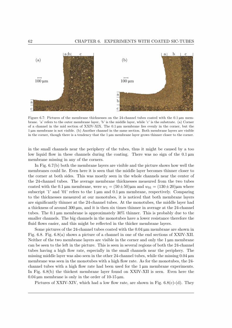
62 CHAPTER 6. EXPERIMENTS WITH COATED SIC-TUBES
(a) (b)
100 µm 100 µm
a b c
a
c
a b c
a
b
c
Figure 6.7: Pictures of the membrane thicknesses on the 24-channel tubes coated with the 0.1 µm mem-brane. ’a’ refers to the outer membrane layer, ’b’ is the middle layer, while ’c’ is the substrate. (a) Cornerof a channel in the mid section of XXIV-XIX. The 0.1 µm membrane lies evenly in the corner, but the1 µm membrane is not visible. (b) Another channel in the same section. Both membrane layers are visiblein the corner, though there is a tendency that the 1 µm membrane layer grows thinner closer to the corner.
in the small channels near the periphery of the tubes, thus it might be caused by a toolow liquid flow in these channels during the coating. There was no sign of the 0.1µmmembrane missing in any of the corners.
In Fig. 6.7(b) both the membrane layers are visible and the picture shows how well themembranes could lie. Even here it is seen that the middle layer becomes thinner closer tothe corner at both sides. This was mostly seen in the whole channels near the center ofthe 24-channel tubes. The average membrane thicknesses measured from the two tubescoated with the 0.1 µm membrane, were w1 = (50±50)µm and w01 = (130±20)µm wheresubscript ’1’ and ’01’ refers to the 1µm and 0.1µm membrane, respectively. Comparingto the thicknesses measured at our monotubes, it is noticed that both membrane layersare significantly thinner at the 24-channel tubes. At the monotubes, the middle layer hada thickness of around 300µm, and it is then six times thinner in average at the 24-channeltubes. The 0.1µm membrane is approximately 30% thinner. This is probably due to thesmaller channels. The big channels in the monotubes have a lower resistance therefore thefluid flows easier, and this might be reflected in the thicker membrane layers.
Some pictures of the 24-channel tubes coated with the 0.04µm membrane are shown inFig. 6.8. Fig. 6.8(a) shows a picture of a channel in one of the end sections of XXIV-XII.Neither of the two membrane layers are visible in the corner and only the 1µm membranecan be seen to the left in the picture. This is seen in several regions of both the 24-channeltubes having a high flow rate, especially in the small channels near the periphery. Themissing middle layer was also seen in the other 24-channel tubes, while the missing 0.04µmmembrane was seen in the monotubes with a high flow rate. As for the monotubes, the 24-channel tubes with a high flow rate had been used for the 1µm membrane experiments.In Fig. 6.8(b) the thickest membrane layer found on XXIV-XII is seen. Even here the0.04 µm membrane is only in the order of 10-15µm.
Pictures of XXIV-XIV, which had a low flow rate, are shown in Fig. 6.8(c)-(d). They
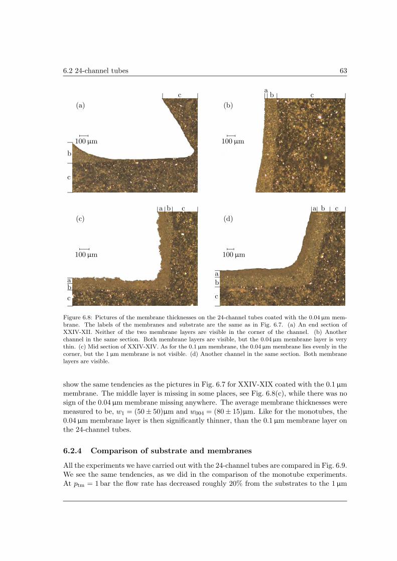
6.2 24-channel tubes 63
(a) (b)
(c) (d)
100 µm 100 µm
100 µm 100 µm
b
c
ca
b c
a b c
ab
c
a b c
ab
c
Figure 6.8: Pictures of the membrane thicknesses on the 24-channel tubes coated with the 0.04 µm mem-brane. The labels of the membranes and substrate are the same as in Fig. 6.7. (a) An end section ofXXIV-XII. Neither of the two membrane layers are visible in the corner of the channel. (b) Anotherchannel in the same section. Both membrane layers are visible, but the 0.04 µm membrane layer is verythin. (c) Mid section of XXIV-XIV. As for the 0.1 µm membrane, the 0.04 µm membrane lies evenly in thecorner, but the 1 µm membrane is not visible. (d) Another channel in the same section. Both membranelayers are visible.
show the same tendencies as the pictures in Fig. 6.7 for XXIV-XIX coated with the 0.1 µmmembrane. The middle layer is missing in some places, see Fig. 6.8(c), while there was nosign of the 0.04µm membrane missing anywhere. The average membrane thicknesses weremeasured to be, w1 = (50± 50)µm and w004 = (80± 15)µm. Like for the monotubes, the0.04 µm membrane layer is then significantly thinner, than the 0.1µm membrane layer onthe 24-channel tubes.
6.2.4 Comparison of substrate and membranes
All the experiments we have carried out with the 24-channel tubes are compared in Fig. 6.9.We see the same tendencies, as we did in the comparison of the monotube experiments.At ptm = 1 bar the flow rate has decreased roughly 20% from the substrates to the 1µm

64 CHAPTER 6. EXPERIMENTS WITH COATED SIC-TUBES
(a)
0
2
4
6
0 0.4 0.8 1.2 1.6
Qp
[m3/h
]
ptm [bar]
x Substratex 1 µm membranex 0.1 µm membranex 0.04 µm membrane
c3 Qp3
[m3/h]
Sub. 0.82 ± 0.02 5.3± 0.3
1 µm 0.82 ± 0.02 4.3± 0.5
0.1 µm 0.93 ± 0.01 2.2± 0.1
0.04 µm 0.93 ± 0.01 2.12 ± 0.06
(b)
Figure 6.9: Comparison of 24-channel tubes. (a) The mean power-law fits from the different experimentsare plotted and the error bars represent the standard deviation on the power-law fits for each of the24-channel tubes. (b) Table containing the average constants including their standard deviations for thepower-law lines on the form Qp = Qp3(ptm/1 bar)c3 . As seen for the monotubes the flow rate is almostequal for the 0.1 µm and the 0.04 µm membrane due to a higher thickness of the 0.1 µm membrane.
membrane experiments, and approximately 60% from the substrate to the 0.1µm and0.04 µm membrane experiments. Again the flow rates through the tubes with these twomembranes are almost equal due the 0.1µm membrane being thicker than the 0.04µmmembrane, as seen in the microscope pictures. The dispersion of the measurements,reflected in the errors bars on the power-law lines, decrease from the substrate experimentsto the membrane experiments, with the exception of the 1µm membrane experiment. Thisis because the 24-channel tubes had been poorly coated with the 1µm membrane. Thereason for this is unknown.
The figure also shows that the flow rate becomes almost linearly related to the trans-membrane pressure in the 0.1µm and 0.04µm membrane experiments, which is especiallyclear when looking at the power c3 from the power-law fits, see Fig. 6.9(b). The closer c3
is to 1, the more linear the fit.
6.3 Summary
Some thin-walled monotubes and some 24-channel tubes are coated with two differenttypes of membrane, a 0.1 µm membrane and a 0.04 µm membrane. Ten monotubes andeight 24-channel tubes are coated with the 0.04µm membrane, while four monotubes andfour 24-channel tubes are coated with the 0.1µm membrane. Experiments with the coatedmonotubes show that Darcy’s law is valid.
In the experiments with both monotubes and 24-channel tubes coated with a 0.04µmmembrane, three of the ten monotubes, and four of the eight 24-channel tubes differ signif-icantly from the others having a surprisingly high flow rate. Bubble point measurementsshowed that the seven tubes had a significantly lower bubble point pressure, compared
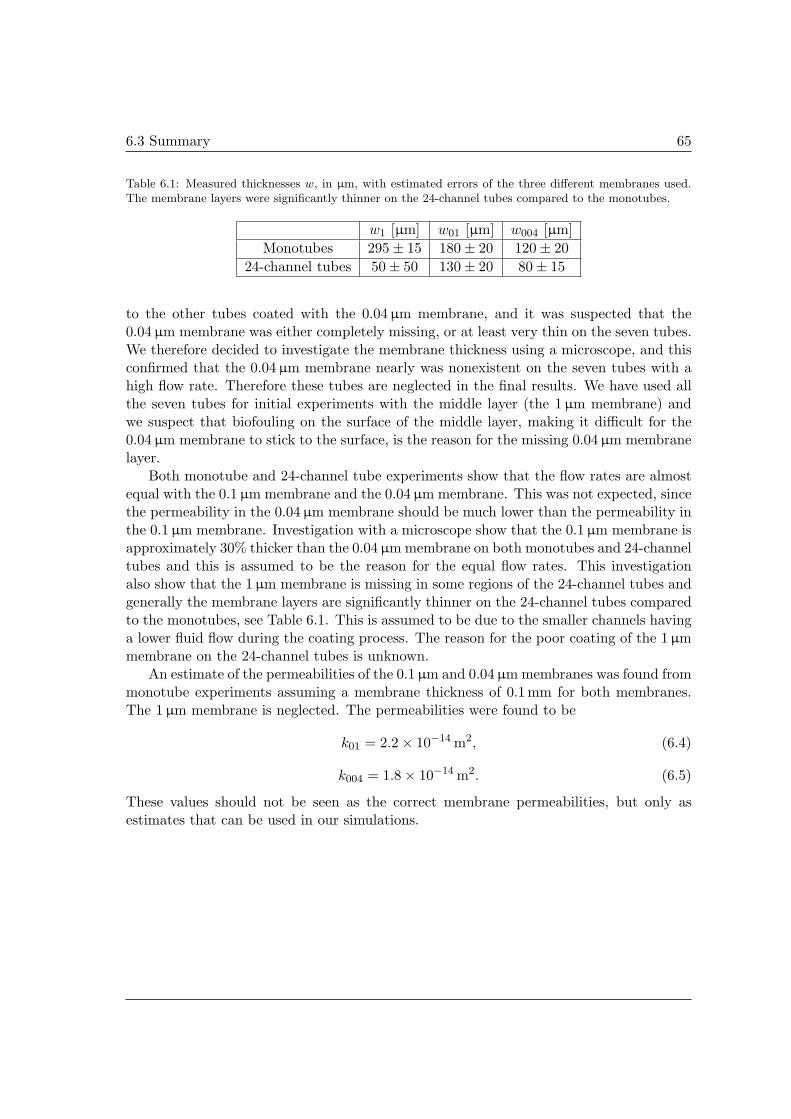
6.3 Summary 65
Table 6.1: Measured thicknesses w, in µm, with estimated errors of the three different membranes used.The membrane layers were significantly thinner on the 24-channel tubes compared to the monotubes.
w1 [µm] w01 [µm] w004 [µm]Monotubes 295± 15 180± 20 120± 20
24-channel tubes 50± 50 130± 20 80± 15
to the other tubes coated with the 0.04 µm membrane, and it was suspected that the0.04 µm membrane was either completely missing, or at least very thin on the seven tubes.We therefore decided to investigate the membrane thickness using a microscope, and thisconfirmed that the 0.04 µm membrane nearly was nonexistent on the seven tubes with ahigh flow rate. Therefore these tubes are neglected in the final results. We have used allthe seven tubes for initial experiments with the middle layer (the 1µm membrane) andwe suspect that biofouling on the surface of the middle layer, making it difficult for the0.04 µm membrane to stick to the surface, is the reason for the missing 0.04 µm membranelayer.
Both monotube and 24-channel tube experiments show that the flow rates are almostequal with the 0.1µm membrane and the 0.04 µm membrane. This was not expected, sincethe permeability in the 0.04 µm membrane should be much lower than the permeability inthe 0.1µm membrane. Investigation with a microscope show that the 0.1µm membrane isapproximately 30% thicker than the 0.04µm membrane on both monotubes and 24-channeltubes and this is assumed to be the reason for the equal flow rates. This investigationalso show that the 1µm membrane is missing in some regions of the 24-channel tubes andgenerally the membrane layers are significantly thinner on the 24-channel tubes comparedto the monotubes, see Table 6.1. This is assumed to be due to the smaller channels havinga lower fluid flow during the coating process. The reason for the poor coating of the 1µmmembrane on the 24-channel tubes is unknown.
An estimate of the permeabilities of the 0.1µm and 0.04µm membranes was found frommonotube experiments assuming a membrane thickness of 0.1mm for both membranes.The 1µm membrane is neglected. The permeabilities were found to be
k01 = 2.2× 10⁻¹⁴ m2, (6.4)
k004 = 1.8× 10⁻¹⁴ m2. (6.5)
These values should not be seen as the correct membrane permeabilities, but only asestimates that can be used in our simulations.

66 CHAPTER 6. EXPERIMENTS WITH COATED SIC-TUBES

Chapter 7
Numerical models and flowsimulations
Two numerical models are developed to describe the flow in porous SiC-tubes. First asimple 2D model is developed based on potential flow theory to describe flow in a cross-section of a tube. The model is implemented in the program Comsol Multiphysicstm
Version 3.4 (Comsol). Second, we develop a 3D model based on equivalent circuit (EC)theory using the program Matlab Version 7.4. 2D EC models are made of the cross-section of a tube and these EC models are connected using the hydraulic resistance in thechannels of the tube. In that way a 3D EC model is created that describes the flow in theentire tube. The two numerical models are presented in the following.
The numerical models are first used to simulate the flow in the substrate and the resultsare compared to the experimental results with substrate tubes presented in Chapter 5. Themodels are extended to include the membrane layer and these results are compared withthe experiments with tubes coated with the 0.04µm membrane presented in Chapter 6.The permeability of the substrate and the 0.04 µm membrane found in the monotubeexperiments will be used in the two models.
7.1 Comsol model
We have made a simple numerical 2D model based on the Laplace equation for the pressure,presented in Section 2.5, and Darcy’s law, Eq. (2.9), for the velocity in the porous SiC.Solving the Laplace equation combined with Darcy’s law is used in [14, 15]. The modelis thus based on potential flow theory. The numerical model is implemented in Comsoland the graphical user interface (GUI) is utilized.
We solved the pressure distribution and flow rate for a monotube analytically in Sec-tion 2.5 and the Comsol simulations of monotubes are therefore left out since they aretrivial. The simulations presented here are made for pure SiC-substrates without mem-brane. The permeability used for the porous SiC is the average permeability found in themonotube experiments ks = 8.3× 10⁻¹³ m2, see Section 5.2.
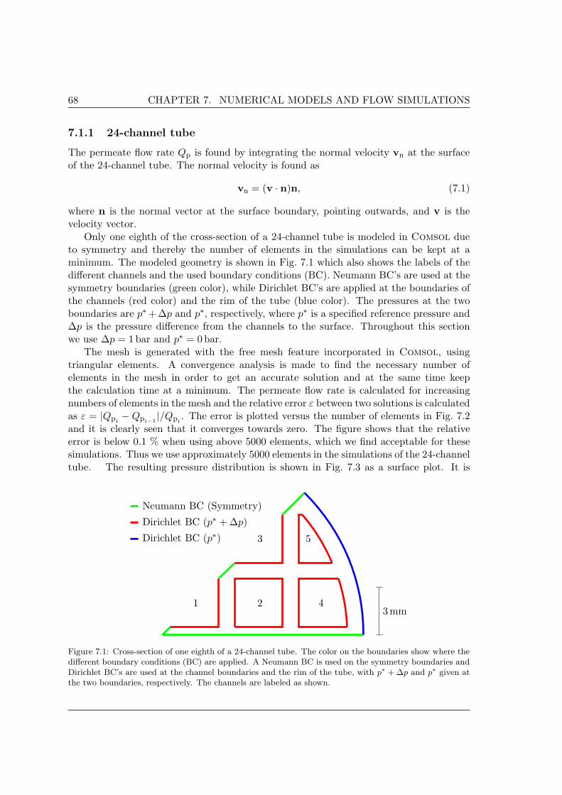
68 CHAPTER 7. NUMERICAL MODELS AND FLOW SIMULATIONS
7.1.1 24-channel tube
The permeate flow rate Qp is found by integrating the normal velocity vn at the surfaceof the 24-channel tube. The normal velocity is found as
vn = (v · n)n, (7.1)
where n is the normal vector at the surface boundary, pointing outwards, and v is thevelocity vector.
Only one eighth of the cross-section of a 24-channel tube is modeled in Comsol dueto symmetry and thereby the number of elements in the simulations can be kept at aminimum. The modeled geometry is shown in Fig. 7.1 which also shows the labels of thedifferent channels and the used boundary conditions (BC). Neumann BC’s are used at thesymmetry boundaries (green color), while Dirichlet BC’s are applied at the boundaries ofthe channels (red color) and the rim of the tube (blue color). The pressures at the twoboundaries are p∗+∆p and p∗, respectively, where p∗ is a specified reference pressure and∆p is the pressure difference from the channels to the surface. Throughout this sectionwe use ∆p = 1bar and p∗ = 0 bar.
The mesh is generated with the free mesh feature incorporated in Comsol, usingtriangular elements. A convergence analysis is made to find the necessary number ofelements in the mesh in order to get an accurate solution and at the same time keepthe calculation time at a minimum. The permeate flow rate is calculated for increasingnumbers of elements in the mesh and the relative error ε between two solutions is calculatedas ε = |Qpi
−Qpi−1|/Qpi
. The error is plotted versus the number of elements in Fig. 7.2and it is clearly seen that it converges towards zero. The figure shows that the relativeerror is below 0.1 % when using above 5000 elements, which we find acceptable for thesesimulations. Thus we use approximately 5000 elements in the simulations of the 24-channeltube. The resulting pressure distribution is shown in Fig. 7.3 as a surface plot. It is
Neumann BC (Symmetry)
Dirichlet BC (p∗ + ∆p)
Dirichlet BC (p∗)
1 2
3
4
5
3mm
Figure 7.1: Cross-section of one eighth of a 24-channel tube. The color on the boundaries show where thedifferent boundary conditions (BC) are applied. A Neumann BC is used on the symmetry boundaries andDirichlet BC’s are used at the channel boundaries and the rim of the tube, with p∗ + ∆p and p∗ given atthe two boundaries, respectively. The channels are labeled as shown.
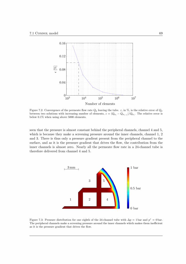
7.1 Comsol model 69
0
0.04
0.08
0.12
0.16
103 104 105 106 107
ε[%
]
Number of elements
Figure 7.2: Convergence of the permeate flow rate Qp leaving the tube. ε, in %, is the relative error of Qp
between two solutions with increasing number of elements, ε = |Qpi− Qpi−1 |/Qpi
. The relative error isbelow 0.1% when using above 5000 elements.
seen that the pressure is almost constant behind the peripheral channels, channel 4 and 5,which is because they make a screening pressure around the inner channels, channel 1, 2and 3. There is thus only a pressure gradient present from the peripheral channel to thesurface, and as it is the pressure gradient that drives the flow, the contribution from theinner channels is almost zero. Nearly all the permeate flow rate in a 24-channel tube istherefore delivered from channel 4 and 5.
0 bar
0.5 bar
1 bar
1 2
3
4
5
3mm
Figure 7.3: Pressure distribution for one eighth of the 24-channel tube with ∆p = 1 bar and p∗ = 0 bar.The peripheral channels make a screening pressure around the inner channels which makes them inefficientas it is the pressure gradient that drives the flow.

70 CHAPTER 7. NUMERICAL MODELS AND FLOW SIMULATIONS
The permeate flow rate calculated from the modeled part of the 24-channel tube ismultiplied by 8 to get the full cross-section and then by L = 305mm to get the flow ratethrough a tube with same length as the ones used in the experiments. The flow rate fromthe simulations is then found to be Qp = 6.51m3/h, of which 98% is delivered from theperipheral channels.
Since we use ∆p = 1 bar and p∗ = 0bar the simulations are made at a transmembranepressure of ptm = 1 bar and the corresponding average flow rate found from the experimentswith the 24-channel tubes was Qp = 5.3m3/h, see Section 5.3. The flow rate calculatedfrom the Comsol model is then 23% higher than the measured flow rate. In the 2Dmodel we assume constant pressure throughout the channels as we neglect the influenceof hydraulic resistance. The experiments with the 24-channel tubes show a significantpressure drop down the length of the tubes and therefore it is expected that the simulationspredict a too high flow rate. Though the simulations do not compensate for the pressuredrop in the channels, they still describe the flow in the porous SiC well. Interestingphenomena, like the peripheral channels screening the inner channels, can be seen usingthis simple numerical model.
7.2 Equivalent circuit model
The nonlinear relation between flow rate and transmembrane pressure seen in the experi-ments with long, thin-walled monotubes and 24-channel tubes cannot be simulated in thesimple 2D Comsol model. We therefore develop a new model using the program Matlab.The analog between the Hagen-Poiseuille law and Ohm’s law described in Section 2.4 willbe used to build a so-called equivalent circuit (EC) model, also called a resistor model, inwhich the hydraulic channel resistance can be taken into account. The hydraulic resistancein the channels is calculated from the energy equation and the friction factor describedin Section 2.3, and the flow in the porous material is assumed to obey Darcy’s law. Thechannels in the tubes are assumed to be smooth in all the simulations. As in the Comsolmodel a permeability of ks = 8.3× 10⁻¹³ m2 is used in the SiC-substrate. Any inlet andoutlet BC’s on the tubes are not included in the model.
7.2.1 Monotube
An EC model of a short monotube is shown in Fig. 7.4. The model describes the flow in amonotube placed in a dead-end setup, as in the conducted experiments. The unknown flowrates and their positive direction, indicated by arrows, are also shown. The length L =305mm of the monotube is discretized into ten parts, each with a length of ∆L = L/10,in order to dissolve the nonlinear relations along the channels sufficiently but still keepthe number of equations at a minimum. The linear relation between pressure differenceand flow rate in the substrate is found from Eq. (2.41),
∆p = RsQ, Rs =η
k
ln(1 + 2wdc
)2πL
, (7.2)

7.2 Equivalent circuit model 71
fRc
Rs
fRc
Rs
fRc
Rs
· · · fRc
Rs
fRc
Rs
fRc
Rs
· · ·
p∗
p∗ + ∆p
Qc1Qc2
Qc3Qc8
Qc9Qc10
Qp1Qp2
Qp3Qp8
Qp9Qp10
Figure 7.4: EC model of a monotube in a dead-end simulation. The length of the monotube is discretizedinto ten parts. The unknown flow rates and their positive directions are shown as well as the nodessymbolized as black squares. p∗ is the reference pressure, ∆p is the pressure difference applied at the inletof the monotube, Rc and Rs are the channel resistance and substrate resistance, respectively, and Qc1 toQc10 and Qp1 to Qp10 are channel flow rates and permeate flow rates.
where Rs is the substrate resistance, dc is the channel diameter and w the wall thickness.The channel flow is found from Eq. (2.26) and repeated here for convenience,
∆p = Rc f(Re) Q2, Rc =L
D5
8ρ
π2, (7.3)
where Rc is the channel resistance. In this model the friction factor varies throughoutthe channel, because of a varying channel flow rate and consequently a varying Reynoldsnumber, and the friction factor is found as described in Section 2.3. The total permeateflow rate delivered from the monotube is found as the sum of the individual ten permeateflow rates Qp1
to Qp10where Qp10
= Qc10 due to the dead-end simulation. Qc1 to Qc10
are the channel flow rates. When the flow rates are known the pressure down the lengthof the channel can be calculated from Eq. (7.3).
The equations describing the flow in a monotube are found by applying Kirchhoff’slaws, described in Section 2.4, to the EC model, see Fig. 7.4. This means that at every node(black squares) the sum of flow rates entering and leaving is zero and in every closed loopthe sum of all pressure differences is also zero. This leads to 19 equations with 19 unknownflow rates Qc1 to Qc10 and Qp1
to Qp9. The equations are implemented in Matlab and
the system of linear and nonlinear equations are solved by Matlab’s nonlinear systemsolver, fsolve.
A reference pressure of p∗ = 0bar is used and different ∆p’s are applied at the inlet ofthe monotube in order to find the relation between permeate flow rate and transmembranepressure. The transmembrane pressure is found as (∆p+pc,10)/2, where pc,10 is the channelpressure found at the end of the monotube. The results of the simulations of a thin-walled monotube are seen in Fig. 7.5 together with the average best-fitted line found inthe monotube experiments. The good agreement seen is expected since the permeabilityused in the simulations is extracted from the monotube experiments. It is seen that thehydraulic channel resistance in the thin-walled monotube is negligible in the simulationsas the relation is linear. This was expected since the experiments with the monotubesshowed a linear relation between flow rate and transmembrane pressure.
The EC model is also applied to a long, thin-walled monotube with a length of L = 1 m.The only difference compared to the short, thin-walled monotube is thus the length. The
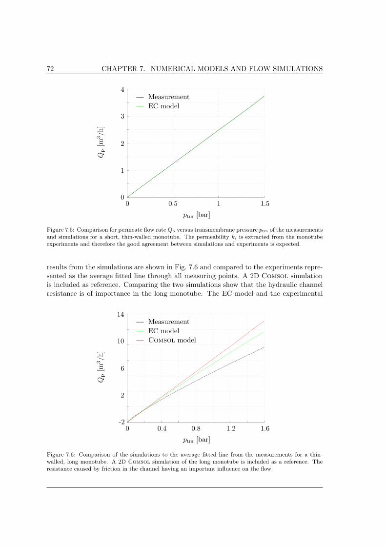
72 CHAPTER 7. NUMERICAL MODELS AND FLOW SIMULATIONS
0
1
2
3
4
0 0.5 1 1.5
Qp
[m3/h
]
ptm [bar]
Measurement
EC model
Figure 7.5: Comparison for permeate flow rate Qp versus transmembrane pressure ptm of the measurementsand simulations for a short, thin-walled monotube. The permeability ks is extracted from the monotubeexperiments and therefore the good agreement between simulations and experiments is expected.
results from the simulations are shown in Fig. 7.6 and compared to the experiments repre-sented as the average fitted line through all measuring points. A 2D Comsol simulationis included as reference. Comparing the two simulations show that the hydraulic channelresistance is of importance in the long monotube. The EC model and the experimental
-2
2
6
10
14
0 0.4 0.8 1.2 1.6
Qp
[m3/h
]
ptm [bar]
Measurement
EC model
Comsol model
Figure 7.6: Comparison of the simulations to the average fitted line from the measurements for a thin-walled, long monotube. A 2D Comsol simulation of the long monotube is included as a reference. Theresistance caused by friction in the channel having an important influence on the flow.
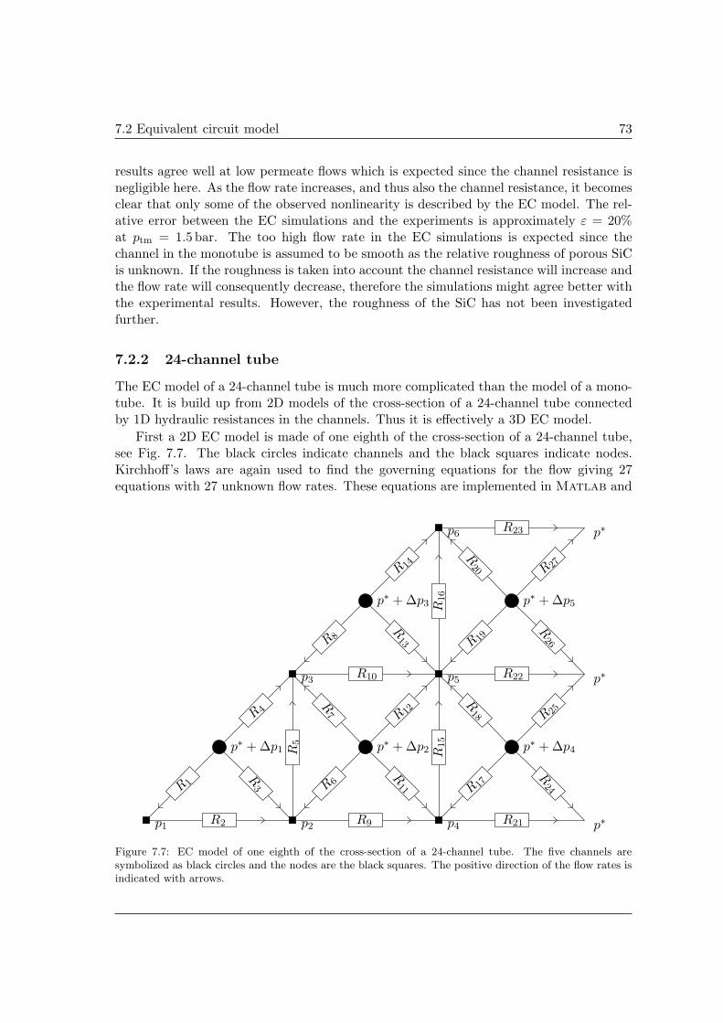
7.2 Equivalent circuit model 73
results agree well at low permeate flows which is expected since the channel resistance isnegligible here. As the flow rate increases, and thus also the channel resistance, it becomesclear that only some of the observed nonlinearity is described by the EC model. The rel-ative error between the EC simulations and the experiments is approximately ε = 20%at ptm = 1.5 bar. The too high flow rate in the EC simulations is expected since thechannel in the monotube is assumed to be smooth as the relative roughness of porous SiCis unknown. If the roughness is taken into account the channel resistance will increase andthe flow rate will consequently decrease, therefore the simulations might agree better withthe experimental results. However, the roughness of the SiC has not been investigatedfurther.
7.2.2 24-channel tube
The EC model of a 24-channel tube is much more complicated than the model of a mono-tube. It is build up from 2D models of the cross-section of a 24-channel tube connectedby 1D hydraulic resistances in the channels. Thus it is effectively a 3D EC model.
First a 2D EC model is made of one eighth of the cross-section of a 24-channel tube,see Fig. 7.7. The black circles indicate channels and the black squares indicate nodes.Kirchhoff’s laws are again used to find the governing equations for the flow giving 27equations with 27 unknown flow rates. These equations are implemented in Matlab and
p1 p2 p4 p∗
p3 p5 p∗
p6 p∗
p∗ + ∆p1 p∗ + ∆p2 p∗ + ∆p4
p∗ + ∆p3 p∗ + ∆p5
R2 R9 R21
R10 R22
R23
R5
R15
R16
R 1
R 4
R 8
R 14
R 6
R 12
R 19
R 27
R 17
R 25
R3
R7
R13
R20
R11
R18
R26
R24
Figure 7.7: EC model of one eighth of the cross-section of a 24-channel tube. The five channels aresymbolized as black circles and the nodes are the black squares. The positive direction of the flow rates isindicated with arrows.
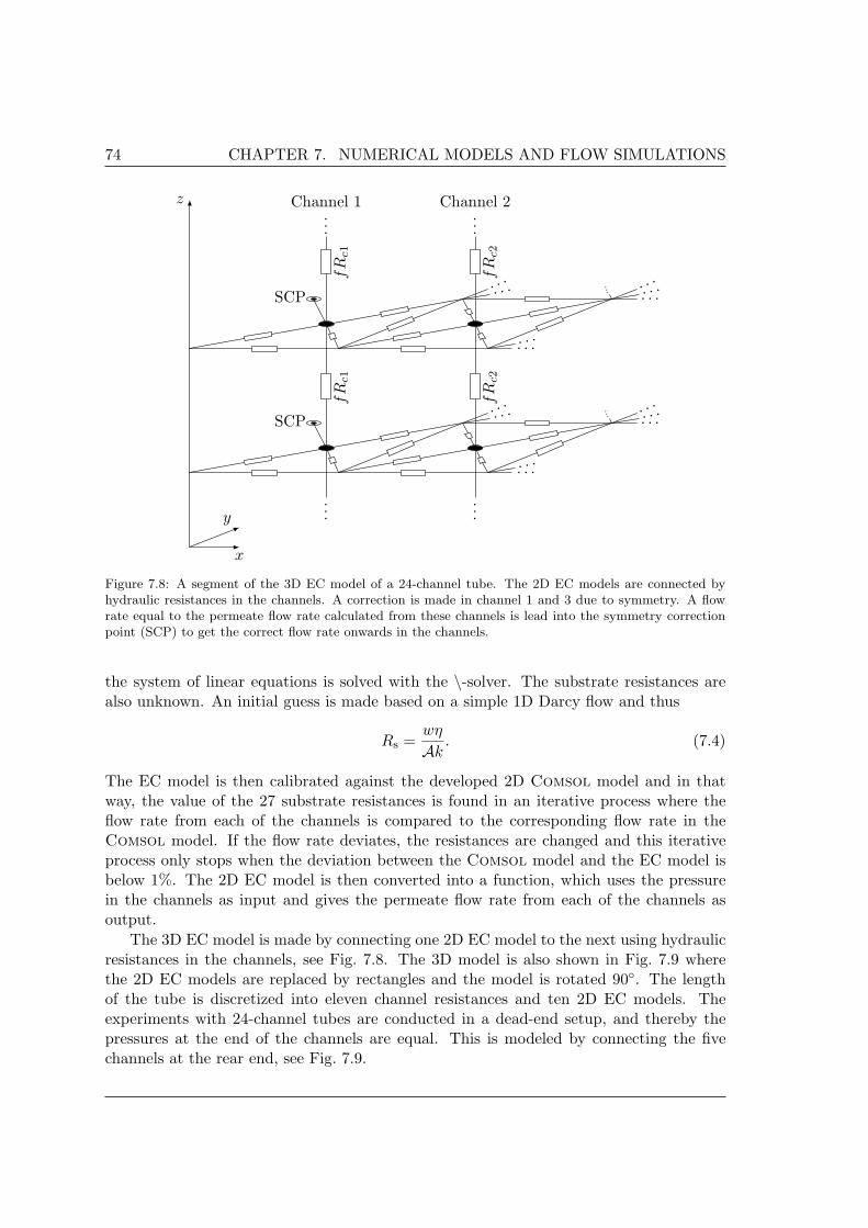
74 CHAPTER 7. NUMERICAL MODELS AND FLOW SIMULATIONS
SCP
· · ·· · ·
· · ·· · ····
···
· · ····
SCP
· · ·· · ·
· · ·· · ····
···
· · ····
···
Channel 1
···
Channel 2
fR
c1
fR
c2
fR
c1
fR
c2
···
···
z
x
y
Figure 7.8: A segment of the 3D EC model of a 24-channel tube. The 2D EC models are connected byhydraulic resistances in the channels. A correction is made in channel 1 and 3 due to symmetry. A flowrate equal to the permeate flow rate calculated from these channels is lead into the symmetry correctionpoint (SCP) to get the correct flow rate onwards in the channels.
the system of linear equations is solved with the \-solver. The substrate resistances arealso unknown. An initial guess is made based on a simple 1D Darcy flow and thus
Rs =wη
Ak. (7.4)
The EC model is then calibrated against the developed 2D Comsol model and in thatway, the value of the 27 substrate resistances is found in an iterative process where theflow rate from each of the channels is compared to the corresponding flow rate in theComsol model. If the flow rate deviates, the resistances are changed and this iterativeprocess only stops when the deviation between the Comsol model and the EC model isbelow 1%. The 2D EC model is then converted into a function, which uses the pressurein the channels as input and gives the permeate flow rate from each of the channels asoutput.
The 3D EC model is made by connecting one 2D EC model to the next using hydraulicresistances in the channels, see Fig. 7.8. The 3D model is also shown in Fig. 7.9 wherethe 2D EC models are replaced by rectangles and the model is rotated 90. The lengthof the tube is discretized into eleven channel resistances and ten 2D EC models. Theexperiments with 24-channel tubes are conducted in a dead-end setup, and thereby thepressures at the end of the channels are equal. This is modeled by connecting the fivechannels at the rear end, see Fig. 7.9.
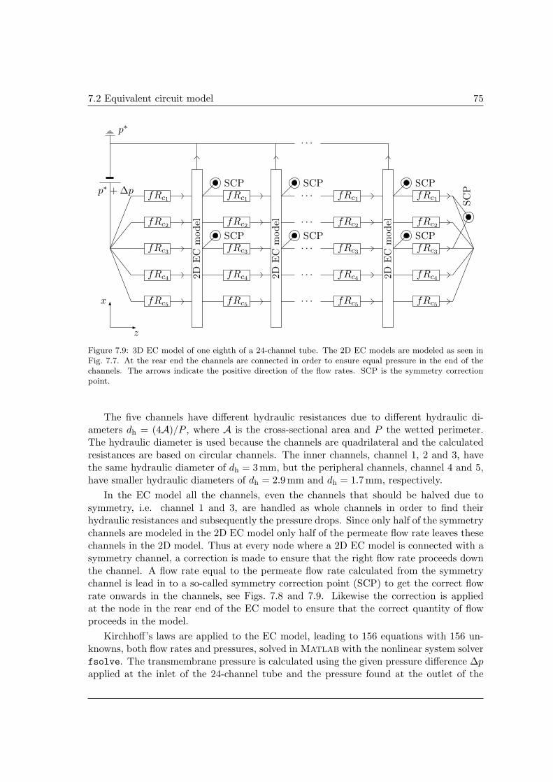
7.2 Equivalent circuit model 75
fRc1
fRc2
fRc3
fRc4
fRc5
fRc1
fRc2
fRc3
fRc4
fRc5
2D
EC
model
2D
EC
model
· · ·
· · ·
· · ·
· · ·
· · ·
fRc1
fRc2
fRc3
fRc4
fRc5
fRc1
fRc2
fRc3
fRc4
fRc5
2D
EC
model
· · ·
p∗
p∗ + ∆p
SC
P
z
x
SCP
SCP
SCP
SCP
SCP
SCP
Figure 7.9: 3D EC model of one eighth of a 24-channel tube. The 2D EC models are modeled as seen inFig. 7.7. At the rear end the channels are connected in order to ensure equal pressure in the end of thechannels. The arrows indicate the positive direction of the flow rates. SCP is the symmetry correctionpoint.
The five channels have different hydraulic resistances due to different hydraulic di-ameters dh = (4A)/P , where A is the cross-sectional area and P the wetted perimeter.The hydraulic diameter is used because the channels are quadrilateral and the calculatedresistances are based on circular channels. The inner channels, channel 1, 2 and 3, havethe same hydraulic diameter of dh = 3 mm, but the peripheral channels, channel 4 and 5,have smaller hydraulic diameters of dh = 2.9 mm and dh = 1.7mm, respectively.
In the EC model all the channels, even the channels that should be halved due tosymmetry, i.e. channel 1 and 3, are handled as whole channels in order to find theirhydraulic resistances and subsequently the pressure drops. Since only half of the symmetrychannels are modeled in the 2D EC model only half of the permeate flow rate leaves thesechannels in the 2D model. Thus at every node where a 2D EC model is connected with asymmetry channel, a correction is made to ensure that the right flow rate proceeds downthe channel. A flow rate equal to the permeate flow rate calculated from the symmetrychannel is lead in to a so-called symmetry correction point (SCP) to get the correct flowrate onwards in the channels, see Figs. 7.8 and 7.9. Likewise the correction is appliedat the node in the rear end of the EC model to ensure that the correct quantity of flowproceeds in the model.
Kirchhoff’s laws are applied to the EC model, leading to 156 equations with 156 un-knowns, both flow rates and pressures, solved in Matlab with the nonlinear system solverfsolve. The transmembrane pressure is calculated using the given pressure difference ∆papplied at the inlet of the 24-channel tube and the pressure found at the outlet of the

76 CHAPTER 7. NUMERICAL MODELS AND FLOW SIMULATIONS
(a) (b)
0.55
0.65
0.75
0.85
0.95
0 0.1 0.2 0.3
pc
[bar
]
` [m]
Chan. 1Chan. 2Chan. 3Chan. 4Chan. 5
0
1
2
3
× 10−2
0 0.1 0.2 0.3
Qp
[m3/(
hm
)]` [m]
Chan. 1
Chan. 2
Chan. 3
Chan. 4
Chan. 5
Figure 7.10: (a) Pressure pc in the channels along the length ` of a 24-channel tube. A massive pressuredrop is seen in the first section of channel 5 while a pressure increase is seen in the last half. (b) Permeateflow rate Qp from the five channels along the length of a 24-channel tube. The peripheral channels delivermost of the total permeate flow while the contribution from the inner most channel, channel 1, is negligible.
tube. The reference pressure is p∗ = 0 bar.The pressure in the channels along the length of the tube is shown in Fig. 7.10(a)
with ∆p = 1bar. The pressure is decreasing nearly linearly in channel 1 while it becomesmore nonlinear in channel 2 and 3 with a total pressure drop of 0.27 bar. In channel 4the pressure decreases significantly in the first half of the tube and then becomes almostconstant in the last half. A massive pressure drop of around 0.4 bar is seen in the first halfof channel 5, and in the last half the pressure then increases to 0.73 bar. The large pressuredrop in channel 4 and 5 is both due to a higher friction as a consequence of the smallerhydraulic diameter and their higher permeate flow rate, compared to the other channels.The pressure increase seen in channel 5 indicates that there is a flow going back throughthe channel in the last half coming from channel 1, 2 and 3. These channels are then feedchannels for the peripheral channels increasing their efficiency regarding permeate flowrate in the last half of the tube.
The amount of permeate flow rate from the five channels along the length of a tube isshown in Fig. 7.10(b) with ∆p = 1 bar. The two peripheral channels, channel 4 and 5, aremuch more efficient than the other channels as it was seen in the Comsol model.
The permeate flow rates from the peripheral channels decrease in the first sections ofthe tube and then increase towards the end of the tube, this is most significant in channel5. This is because of the dead-end simulation in which all the flow has to permeate throughthe porous walls. The easiest way for the fluid in the inner channels to permeate out ofthe tube is then to flow back through the peripheral channels and permeate out of thewalls here.
The pressure drop ∆ptube lengthwise in a 24-channel tube is estimated at differentpermeate flow rates and compared to the measured data, see Fig. 7.11. The measureddata is represented as the average fitted line through all the measuring points. Fig. 7.11shows that the simulated pressure drop is comparable to the measured pressure drop, but
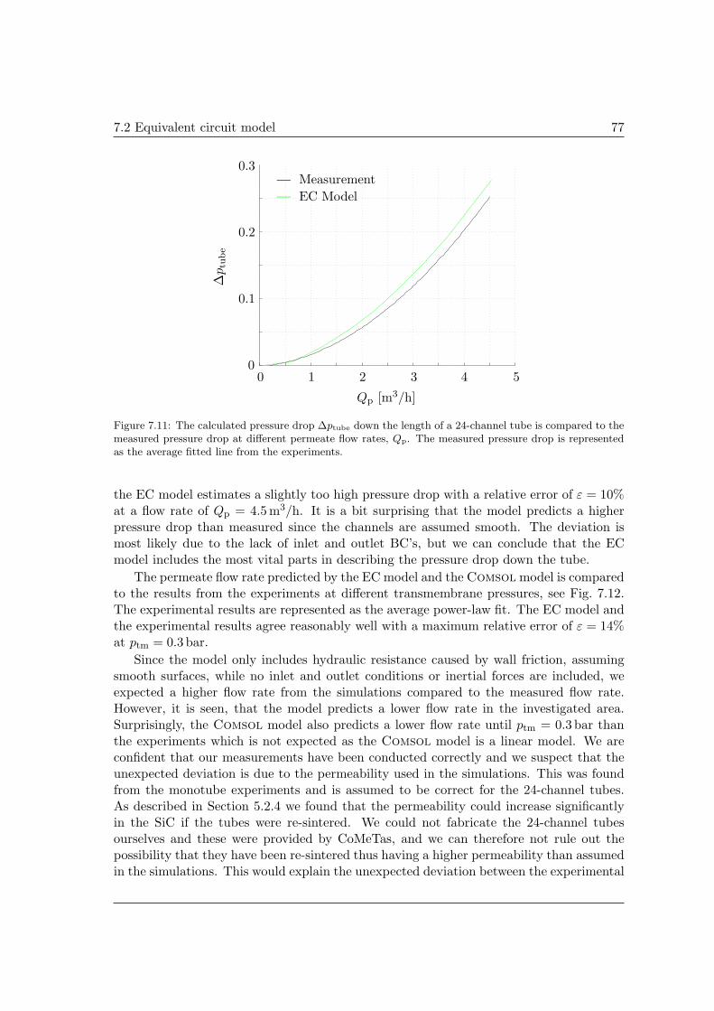
7.2 Equivalent circuit model 77
0
0.1
0.2
0.3
0 1 2 3 4 5
∆ptu
be
Qp [m3/h]
Measurement
EC Model
Figure 7.11: The calculated pressure drop ∆ptube down the length of a 24-channel tube is compared to themeasured pressure drop at different permeate flow rates, Qp. The measured pressure drop is representedas the average fitted line from the experiments.
the EC model estimates a slightly too high pressure drop with a relative error of ε = 10%at a flow rate of Qp = 4.5 m3/h. It is a bit surprising that the model predicts a higherpressure drop than measured since the channels are assumed smooth. The deviation ismost likely due to the lack of inlet and outlet BC’s, but we can conclude that the ECmodel includes the most vital parts in describing the pressure drop down the tube.
The permeate flow rate predicted by the EC model and the Comsol model is comparedto the results from the experiments at different transmembrane pressures, see Fig. 7.12.The experimental results are represented as the average power-law fit. The EC model andthe experimental results agree reasonably well with a maximum relative error of ε = 14%at ptm = 0.3 bar.
Since the model only includes hydraulic resistance caused by wall friction, assumingsmooth surfaces, while no inlet and outlet conditions or inertial forces are included, weexpected a higher flow rate from the simulations compared to the measured flow rate.However, it is seen, that the model predicts a lower flow rate in the investigated area.Surprisingly, the Comsol model also predicts a lower flow rate until ptm = 0.3 bar thanthe experiments which is not expected as the Comsol model is a linear model. We areconfident that our measurements have been conducted correctly and we suspect that theunexpected deviation is due to the permeability used in the simulations. This was foundfrom the monotube experiments and is assumed to be correct for the 24-channel tubes.As described in Section 5.2.4 we found that the permeability could increase significantlyin the SiC if the tubes were re-sintered. We could not fabricate the 24-channel tubesourselves and these were provided by CoMeTas, and we can therefore not rule out thepossibility that they have been re-sintered thus having a higher permeability than assumedin the simulations. This would explain the unexpected deviation between the experimental
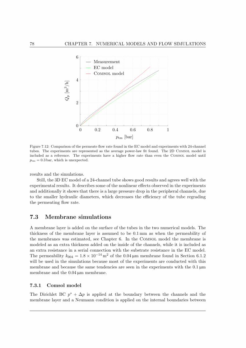
78 CHAPTER 7. NUMERICAL MODELS AND FLOW SIMULATIONS
0
2
4
6
0 0.2 0.4 0.6 0.8 1
Qp
[m3/h
]
ptm [bar]
Measurement
EC model
Comsol model
Figure 7.12: Comparison of the permeate flow rate found in the EC model and experiments with 24-channeltubes. The experiments are represented as the average power-law fit found. The 2D Comsol model isincluded as a reference. The experiments have a higher flow rate than even the Comsol model untilptm = 0.3 bar, which is unexpected.
results and the simulations.Still, the 3D EC model of a 24-channel tube shows good results and agrees well with the
experimental results. It describes some of the nonlinear effects observed in the experimentsand additionally it shows that there is a large pressure drop in the peripheral channels, dueto the smaller hydraulic diameters, which decreases the efficiency of the tube regradingthe permeating flow rate.
7.3 Membrane simulations
A membrane layer is added on the surface of the tubes in the two numerical models. Thethickness of the membrane layer is assumed to be 0.1mm as when the permeability ofthe membranes was estimated, see Chapter 6. In the Comsol model the membrane ismodeled as an extra thickness added on the inside of the channels, while it is included asan extra resistance in a serial connection with the substrate resistance in the EC model.The permeability k004 = 1.8× 10⁻¹⁴ m2 of the 0.04µm membrane found in Section 6.1.2will be used in the simulations because most of the experiments are conducted with thismembrane and because the same tendencies are seen in the experiments with the 0.1µmmembrane and the 0.04µm membrane.
7.3.1 Comsol model
The Dirichlet BC p∗ + ∆p is applied at the boundary between the channels and themembrane layer and a Neumann condition is applied on the internal boundaries between
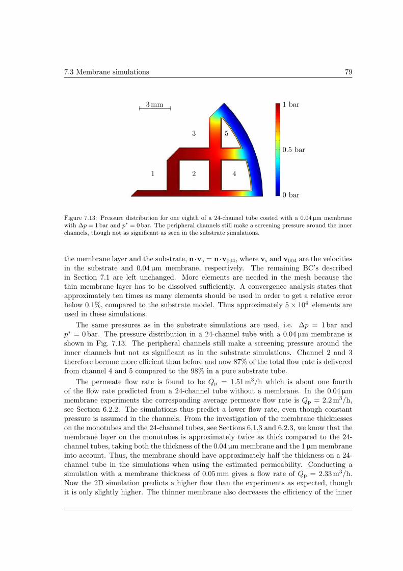
7.3 Membrane simulations 79
0 bar
0.5 bar
1 bar
1 2
3
4
5
3mm
Figure 7.13: Pressure distribution for one eighth of a 24-channel tube coated with a 0.04 µm membranewith ∆p = 1bar and p∗ = 0 bar. The peripheral channels still make a screening pressure around the innerchannels, though not as significant as seen in the substrate simulations.
the membrane layer and the substrate, n ·vs = n ·v004, where vs and v004 are the velocitiesin the substrate and 0.04 µm membrane, respectively. The remaining BC’s describedin Section 7.1 are left unchanged. More elements are needed in the mesh because thethin membrane layer has to be dissolved sufficiently. A convergence analysis states thatapproximately ten times as many elements should be used in order to get a relative errorbelow 0.1%, compared to the substrate model. Thus approximately 5× 10⁴ elements areused in these simulations.
The same pressures as in the substrate simulations are used, i.e. ∆p = 1bar andp∗ = 0 bar. The pressure distribution in a 24-channel tube with a 0.04µm membrane isshown in Fig. 7.13. The peripheral channels still make a screening pressure around theinner channels but not as significant as in the substrate simulations. Channel 2 and 3therefore become more efficient than before and now 87% of the total flow rate is deliveredfrom channel 4 and 5 compared to the 98% in a pure substrate tube.
The permeate flow rate is found to be Qp = 1.51m3/h which is about one fourthof the flow rate predicted from a 24-channel tube without a membrane. In the 0.04 µmmembrane experiments the corresponding average permeate flow rate is Qp = 2.2m3/h,see Section 6.2.2. The simulations thus predict a lower flow rate, even though constantpressure is assumed in the channels. From the investigation of the membrane thicknesseson the monotubes and the 24-channel tubes, see Sections 6.1.3 and 6.2.3, we know that themembrane layer on the monotubes is approximately twice as thick compared to the 24-channel tubes, taking both the thickness of the 0.04 µm membrane and the 1µm membraneinto account. Thus, the membrane should have approximately half the thickness on a 24-channel tube in the simulations when using the estimated permeability. Conducting asimulation with a membrane thickness of 0.05 mm gives a flow rate of Qp = 2.33m3/h.Now the 2D simulation predicts a higher flow than the experiments as expected, thoughit is only slightly higher. The thinner membrane also decreases the efficiency of the inner
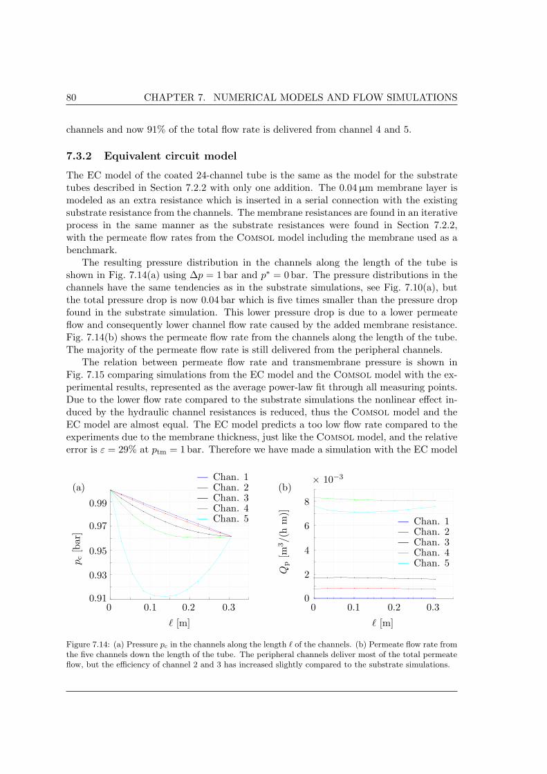
80 CHAPTER 7. NUMERICAL MODELS AND FLOW SIMULATIONS
channels and now 91% of the total flow rate is delivered from channel 4 and 5.
7.3.2 Equivalent circuit model
The EC model of the coated 24-channel tube is the same as the model for the substratetubes described in Section 7.2.2 with only one addition. The 0.04 µm membrane layer ismodeled as an extra resistance which is inserted in a serial connection with the existingsubstrate resistance from the channels. The membrane resistances are found in an iterativeprocess in the same manner as the substrate resistances were found in Section 7.2.2,with the permeate flow rates from the Comsol model including the membrane used as abenchmark.
The resulting pressure distribution in the channels along the length of the tube isshown in Fig. 7.14(a) using ∆p = 1 bar and p∗ = 0 bar. The pressure distributions in thechannels have the same tendencies as in the substrate simulations, see Fig. 7.10(a), butthe total pressure drop is now 0.04 bar which is five times smaller than the pressure dropfound in the substrate simulation. This lower pressure drop is due to a lower permeateflow and consequently lower channel flow rate caused by the added membrane resistance.Fig. 7.14(b) shows the permeate flow rate from the channels along the length of the tube.The majority of the permeate flow rate is still delivered from the peripheral channels.
The relation between permeate flow rate and transmembrane pressure is shown inFig. 7.15 comparing simulations from the EC model and the Comsol model with the ex-perimental results, represented as the average power-law fit through all measuring points.Due to the lower flow rate compared to the substrate simulations the nonlinear effect in-duced by the hydraulic channel resistances is reduced, thus the Comsol model and theEC model are almost equal. The EC model predicts a too low flow rate compared to theexperiments due to the membrane thickness, just like the Comsol model, and the relativeerror is ε = 29% at ptm = 1 bar. Therefore we have made a simulation with the EC model
(a) (b)
0.91
0.93
0.95
0.97
0.99
0 0.1 0.2 0.3
pc
[bar
]
` [m]
Chan. 1Chan. 2Chan. 3Chan. 4Chan. 5
0
2
4
6
8
× 10−3
0 0.1 0.2 0.3
Qp
[m3/(
hm
)]
` [m]
Chan. 1Chan. 2Chan. 3Chan. 4Chan. 5
Figure 7.14: (a) Pressure pc in the channels along the length ` of the channels. (b) Permeate flow rate fromthe five channels down the length of the tube. The peripheral channels deliver most of the total permeateflow, but the efficiency of channel 2 and 3 has increased slightly compared to the substrate simulations.

7.4 Summary 81
0
1
2
3
0 0.5 1 1.5
Qp
[m3/h
]
ptm [bar]
Measurement
EC model
Comsol model
EC model, k004/2
Figure 7.15: Comparison of the permeate flow rate found in the EC model and experiments with 24-channeltubes coated with the 0.04 µm membrane. The experiments are represented as the average power-law fit.The 2D Comsol model is included as a reference. Both numerical simulations lie significantly lower thanthe experimental results due to a wrong membrane thickness in the simulations. A simulation is alsoconducted with the EC model using half the membrane thickness which agrees well with the experiments.
using half the membrane thickness also shown in Fig. 7.15. This simulation agrees verywell with the experimental results with a relative error of only ε = 3% at ptm = 1 bar. Stillthe simulations are expected to lie even higher due to the lack of inlet and outlet BC’s andinertia. Thus the membrane thickness should maybe be even thinner in the simulations.This is hard to determine, however, since the membrane thickness was so different betweenthe monotubes and 24-channel tubes. Furthermore the quality of the 1µm membrane waspoor on the 24-channel tubes making it even more difficult to get the simulations and theexperiments to agree.
Based on these considerations and the presented results we thus conclude that theEC model of a 24-channel tube describes the flow well. The deviations seen betweenthe simulations and the experiments are expected to be mainly due to the quality andthickness of the membrane layers on the 24-channel tubes used in the experimental work.
7.4 Summary
We have developed two numerical models describing flow in porous SiC-tubes. Bothmodels use the permeability for the SiC-substrate and the estimated permeability for the0.04 µm membrane found in the monotube experiments. The first model is a simple 2Dmodel made in Comsol based on potential flow theory using the Laplace equation forthe pressure and Darcy’s law for the velocity in the porous SiC. The other model is a3D equivalent circuit model based on the analogy between the Hagen-Poiseuille law andOhm’s law from electricity. This model includes the hydraulic resistance in the channels

82 CHAPTER 7. NUMERICAL MODELS AND FLOW SIMULATIONS
of the tubes due to wall friction, assuming smooth channels.The 2D Comsol model of the pure 24-channel substrate show that the peripheral
channels make a screening pressure of the inner channel. This means that 98% of thepermeate flow rate from a 24-channel tube is delivered by the peripheral channels in thesubstrate tubes while the peripheral channels deliver 87% of the flow rate in tubes coatedwith the 0.04µm membrane. Thus the inner channels are almost redundant in the 24-channel tube.
We found that the EC model predict the pressure drop down the length of a 24-channeltube well compared to the measured pressure drop. Furthermore a significant pressuredrop was found in the peripheral channels due to small hydraulic diameters and higherflow rates compared to the inner channels. This pressure drop decreases the efficiencyof the tubes because the peripheral channels deliver the majority of the permeate flow.The EC model predicts a lower permeate flow rate than seen in the experiments withthe 24-channel substrates with a maximum deviation of ε = 14%. It was expected thatthe model predicted a higher flow rate since the channels are assumed smooth and inletand outlet BC’s and inertia are neglected. Also the Comsol model predicts a lower flowrate than the experiments until ptm = 0.3 bar which is unexpected as it is a linear modeland thus uses the most optimal conditions. We suspect that this is due to the 24-channeltubes having a higher permeability than expected, which might be because they have beenre-sintered, but this is unknown to us.
The simulations with 24-channel tubes coated with 0.04µm membrane give a signif-icantly lower flow rate than seen in the experiments with a relative error of ε = 29% atptm = 1 bar. The lower flow rate is due to the assumption of equal thickness of the 0.04µmmembrane on the 24-channel tubes and on the monotubes. Investigations of the membranehave shown that it is only approximately half as thick on 24-channel tubes compared tomonotubes and using half the thickness in the EC simulations give good agreement withthe experiments.

Chapter 8
Geometrical optimization
The two numerical models presented in Chapter 7 will be used to optimize the geometryof the SiC focusing on increasing the permeate flow rate. The optimization process is doneassuming clean, demineralized water, and therefore no considerations concerning the sizeof the membrane area (the surface area of the channels in the tubes) or contaminated fluidare made.
First, we make some simple optimization suggestions of a 24-channel tube based onthe flow phenomena seen in Chapter 7. We will therefore focus on increasing the surfacearea in order to avoid screening of the inner channels and we will increase the size ofthe channels in order to decrease the pressure drop throughout the length of the tubes.The optimized geometries will be compared to the simulations of the original 24-channeltube and both the Comsol model and the EC model will be used to estimate the flowrate delivered from these new design suggestions. Both substrate and 0.04µm membranesimulations will be made but only the results will be presented.
Secondly, we compare the achieved results with data from a standard membrane usedby CoMeTas, the so-called COM-144-865-(2*2)-0.04, using both experimental results forthe original 24-channel tubes and the simulations of the best optimized geometry. Somesuggestions on how to improve the large standard membrane used by CoMeTas are pre-sented and the efficiency is compared to simulations of the original membrane.
We have decided that the new geometries should have a uniform wall thickness tominimize the risk of cracks appearing in the drying or sintering process. Furthermore, theratio between wall thickness and channel dimensions is kept above 0.25 for the structureto be self-sustaining when extruded, [22]. We are thankful to Johnny Marcher, technicaldirector at LiqTech, for good advice and technical discussions concerning limitations andpossibilities of new designs.
8.1 Optimizing surface area
The results from the Comsol simulations of a 24-channel tube with length L = 305 mm arelisted in Table 8.1 and these results will be used as comparison values for the optimizationsuggestions. Unless otherwise noted the following parameters will be used throughout

84 CHAPTER 8. GEOMETRICAL OPTIMIZATION
Table 8.1: (a) The permeate flow rate leaving the original 24-channel tube with L = 305 mm uncoated andcoated with a 0.04 µm membrane. (b) The surface and membrane areas of the tube.
(a) Qp [m3/h] (b) A [m2]Substrate 6.51 Surface area 2.39× 10⁻²
0.04µm membrane 1.51 Membrane area 1.08× 10⁻¹
this chapter: L = 305 mm, do = 25 mm, ∆p = 1 bar, p∗ = 0bar, ks = 8.3× 10⁻¹³ m2,k004 = 1.8× 10⁻¹⁴ m2 and w004 = 0.1mm, where do is the outer diameter of the tubes andw004 is the thickness of the 0.04µm membrane.
In the original 24-channel tube the permeate flow rate is largely delivered by the pe-ripheral channels because the inner channels are screened by the pressure in these channels,see Section 7.2.2. The efficiency of the 24-channel tube can then be increased by reducingthe screening, which can be done by increasing the surface area. The simplest way to dothis is by making a cut into the original geometry of the 24-channel tube, see Fig. 8.1where the pressure distribution is shown for such a suggestion. Fig. 8.1(a) is the pressuredistribution in a pure substrate while the substrate is coated with the 0.04µm membranein Fig. 8.1(b). In this design the cut is one channel wide and three channels deep and allthe walls still have a thickness of 1 mm. Some of the inner channels now contribute to thepermeate flow rate in both simulations which can be seen from the pressure gradient. Thepermeate flow rate for both the substrate and the tube coated with a 0.04 µm membranehas increased by 29%, see Fig. 8.1(c), compared to the original 24-channel tube. Thus arelatively simple change in the geometry leads to a significant increase in the permeate flow
(a) (b)
0 bar
0.5 bar
1 bar
0 bar
0.5 bar
1 bar
(c)
Qp [m3/h]
Substrate 8.390.04 µm membrane 1.93
(d)
A [m2]
Surface area 3.11 × 10⁻²
Membrane area 9.73 × 10⁻²
7 mm 7mm
Figure 8.1: Pressure distribution in a 24-channel tube with a cut which is three channels deep and onechannel wide. The thickness of the walls is still w = 1 mm and the length is L = 305mm. (a) The pressuredistribution in a substrate tube. (b) Tube coated with 0.04 µm membrane. (c) The permeate flow ratesfor both simulations. (d) Surface and membrane areas of the new geometry.
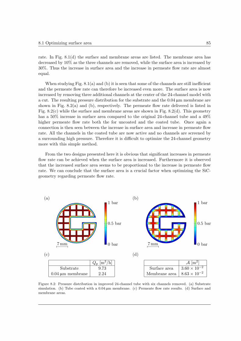
8.1 Optimizing surface area 85
rate. In Fig. 8.1(d) the surface and membrane areas are listed. The membrane area hasdecreased by 10% as the three channels are removed, while the surface area is increased by30%. Thus the increase in surface area and the increase in permeate flow rate are almostequal.
When studying Fig. 8.1(a) and (b) it is seen that some of the channels are still inefficientand the permeate flow rate can therefore be increased even more. The surface area is nowincreased by removing three additional channels at the center of the 24-channel model witha cut. The resulting pressure distribution for the substrate and the 0.04 µm membrane areshown in Fig. 8.2(a) and (b), respectively. The permeate flow rate delivered is listed inFig. 8.2(c) while the surface and membrane areas are shown in Fig. 8.2(d). This geometryhas a 50% increase in surface area compared to the original 24-channel tube and a 49%higher permeate flow rate both the for uncoated and the coated tube. Once again aconnection is then seen between the increase in surface area and increase in permeate flowrate. All the channels in the coated tube are now active and no channels are screened bya surrounding high pressure. Therefore it is difficult to optimize the 24-channel geometrymore with this simple method.
From the two designs presented here it is obvious that significant increases in permeateflow rate can be achieved when the surface area is increased. Furthermore it is observedthat the increased surface area seems to be proportional to the increase in permeate flowrate. We can conclude that the surface area is a crucial factor when optimizing the SiC-geometry regarding permeate flow rate.
(a) (b)
0 bar
0.5 bar
1 bar
0 bar
0.5 bar
1 bar
(c)
Qp [m3/h]
Substrate 9.730.04 µm membrane 2.24
(d)
A [m2]
Surface area 3.60 × 10⁻²
Membrane area 8.63 × 10⁻²
7 mm 7mm
Figure 8.2: Pressure distribution in improved 24-channel tube with six channels removed. (a) Substratesimulation. (b) Tube coated with a 0.04 µm membrane. (c) Permeate flow rate results. (d) Surface andmembrane areas.

86 CHAPTER 8. GEOMETRICAL OPTIMIZATION
8.2 Optimizing channel dimensions
In the original 24-channel tube the peripheral channels have smaller hydraulic diameterscompared to the inner channels. Since the peripheral channels deliver the majority ofthe permeate flow rate these channels should have a large hydraulic diameter to minimizethe pressure drop down the length of the channels. However, we cannot just increase thesize of the channels if the new designs shall be possible to extrude. The ratio betweenwall thickness w and the hydraulic diameter dh of the channels should not be lower thanw/dh = 0.25 for the structure to be self-sustaining when extruded, [22]. Since we want tokeep the wall thickness small in order to have a high permeate flow rate this limits thesize of the channels. For simplicity the wall thickness is kept constant at w = 1mm in thedesigns presented here.
A design is made with a new channel distribution and the resulting pressure distri-bution is seen in Fig. 8.3(a) and (b), for the substrate tube and the tube coated with a0.04 µm membrane, respectively. The position of the channels has been changed so thatthey follow the geometry and hereby we avoid the small channels near the surface as seenin the 24-channel geometry. The permeate flow rates are listed in Fig. 8.3(c) while thesurface and membrane areas are shown in Fig. 8.3(d). The hydraulic diameters of thechannels are dh = 3.0mm in the inner channels, dh = 3.8 mm in the second row of chan-nels, and dh = 3.5mm in the peripheral channels. The size of the smallest channels is thencomparable to the biggest channels in the original 24-channel tube. The wall thicknessis w = 1 mm and a total of 21 channels are present in this new design, thus naming it a21-channel tube.
The surface area is identical to that of a 24-channel tube, but the membrane area is
(a) (b)
0 bar
0.5 bar
1 bar
0 bar
0.5 bar
1 bar
(c)
Qp [m3/h]
Substrate 6.690.04 µm membrane 1.41
(d)
A [m2]
Surface area 2.39 × 10⁻²
Membrane area 9.49 × 10⁻²
7 mm 7mm
Figure 8.3: Pressure distribution in a new design named a 21-channel tube due to the 21 channels. (a)Substrate tube. (b) Coated with a 0.04 µm membrane. (c) Permeate flow rates for the two simulations.(d) Membrane and surface areas of the geometry.
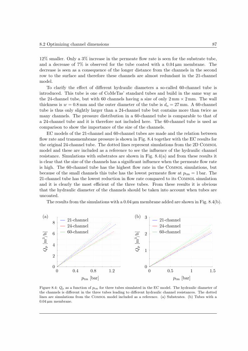
8.2 Optimizing channel dimensions 87
12% smaller. Only a 3% increase in the permeate flow rate is seen for the substrate tube,and a decrease of 7% is observed for the tube coated with a 0.04µm membrane. Thedecrease is seen as a consequence of the longer distance from the channels in the secondrow to the surface and therefore these channels are almost redundant in the 21-channelmodel.
To clarify the effect of different hydraulic diameters a so-called 60-channel tube isintroduced. This tube is one of CoMeTas’ standard tubes and build in the same way asthe 24-channel tube, but with 60 channels having a size of only 2 mm× 2mm. The wallthickness is w = 0.8mm and the outer diameter of the tube is do = 27mm. A 60-channeltube is thus only slightly larger than a 24-channel tube but contains more than twice asmany channels. The pressure distribution in a 60-channel tube is comparable to that ofa 24-channel tube and it is therefore not included here. The 60-channel tube is used ascomparison to show the importance of the size of the channels.
EC models of the 21-channel and 60-channel tubes are made and the relation betweenflow rate and transmembrane pressure is shown in Fig. 8.4 together with the EC results forthe original 24-channel tube. The dotted lines represent simulations from the 2D Comsolmodel and these are included as a reference to see the influence of the hydraulic channelresistance. Simulations with substrates are shown in Fig. 8.4(a) and from these results itis clear that the size of the channels has a significant influence when the permeate flow rateis high. The 60-channel tube has the highest flow rate in the Comsol simulations, butbecause of the small channels this tube has the lowest permeate flow at ptm = 1 bar. The21-channel tube has the lowest reduction in flow rate compared to its Comsol simulationand it is clearly the most efficient of the three tubes. From these results it is obviousthat the hydraulic diameter of the channels should be taken into account when tubes areuncoated.
The results from the simulations with a 0.04µm membrane added are shown in Fig. 8.4(b).
(a) (b)
0
2
4
6
8
0 0.4 0.8 1.2
Qp
[m3/h
]
ptm [bar]
21-channel
24-channel
60-channel
0
1
2
3
0 0.5 1 1.5
Qp
[m3/h
]
ptm [bar]
21-channel
24-channel
60-channel
Figure 8.4: Qp as a function of ptm for three tubes simulated in the EC model. The hydraulic diameter ofthe channels is different in the three tubes leading to different hydraulic channel resistances. The dottedlines are simulations from the Comsol model included as a reference. (a) Substrates. (b) Tubes with a0.04 µm membrane.
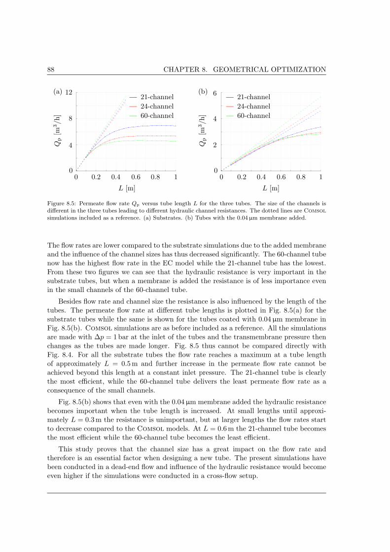
88 CHAPTER 8. GEOMETRICAL OPTIMIZATION
(a) (b)
0
4
8
12
0 0.2 0.4 0.6 0.8 1
Qp
[m3/h
]
L [m]
21-channel
24-channel
60-channel
0
2
4
6
0 0.2 0.4 0.6 0.8 1
Qp
[m3/h
]
L [m]
21-channel
24-channel
60-channel
Figure 8.5: Permeate flow rate Qp versus tube length L for the three tubes. The size of the channels isdifferent in the three tubes leading to different hydraulic channel resistances. The dotted lines are Comsolsimulations included as a reference. (a) Substrates. (b) Tubes with the 0.04 µm membrane added.
The flow rates are lower compared to the substrate simulations due to the added membraneand the influence of the channel sizes has thus decreased significantly. The 60-channel tubenow has the highest flow rate in the EC model while the 21-channel tube has the lowest.From these two figures we can see that the hydraulic resistance is very important in thesubstrate tubes, but when a membrane is added the resistance is of less importance evenin the small channels of the 60-channel tube.
Besides flow rate and channel size the resistance is also influenced by the length of thetubes. The permeate flow rate at different tube lengths is plotted in Fig. 8.5(a) for thesubstrate tubes while the same is shown for the tubes coated with 0.04µm membrane inFig. 8.5(b). Comsol simulations are as before included as a reference. All the simulationsare made with ∆p = 1 bar at the inlet of the tubes and the transmembrane pressure thenchanges as the tubes are made longer. Fig. 8.5 thus cannot be compared directly withFig. 8.4. For all the substrate tubes the flow rate reaches a maximum at a tube lengthof approximately L = 0.5 m and further increase in the permeate flow rate cannot beachieved beyond this length at a constant inlet pressure. The 21-channel tube is clearlythe most efficient, while the 60-channel tube delivers the least permeate flow rate as aconsequence of the small channels.
Fig. 8.5(b) shows that even with the 0.04µm membrane added the hydraulic resistancebecomes important when the tube length is increased. At small lengths until approxi-mately L = 0.3m the resistance is unimportant, but at larger lengths the flow rates startto decrease compared to the Comsol models. At L = 0.6m the 21-channel tube becomesthe most efficient while the 60-channel tube becomes the least efficient.
This study proves that the channel size has a great impact on the flow rate andtherefore is an essential factor when designing a new tube. The present simulations havebeen conducted in a dead-end flow and influence of the hydraulic resistance would becomeeven higher if the simulations were conducted in a cross-flow setup.
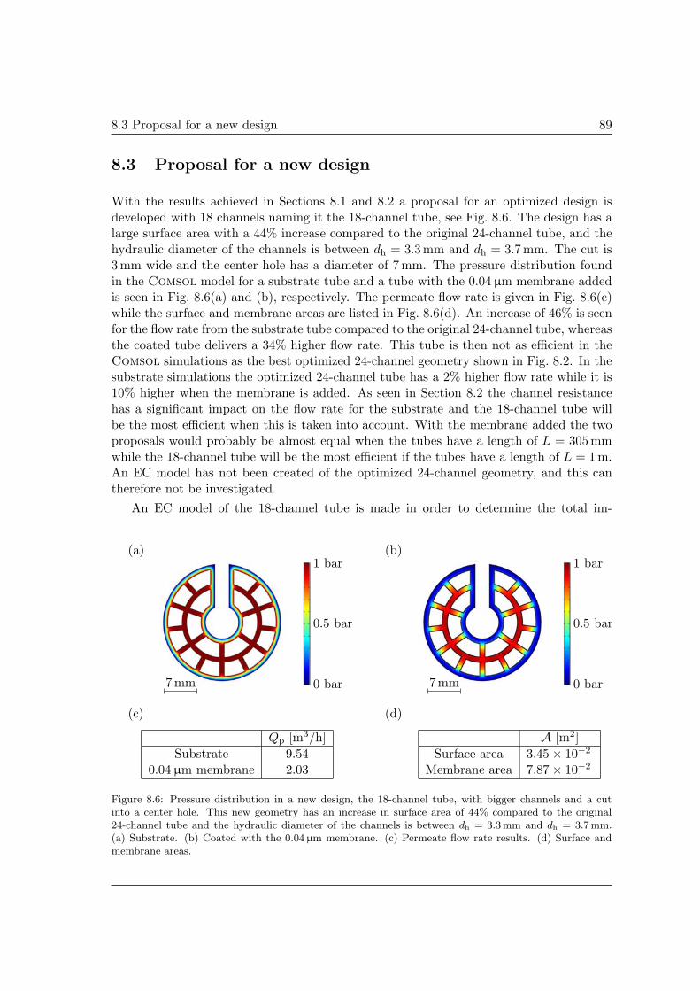
8.3 Proposal for a new design 89
8.3 Proposal for a new design
With the results achieved in Sections 8.1 and 8.2 a proposal for an optimized design isdeveloped with 18 channels naming it the 18-channel tube, see Fig. 8.6. The design has alarge surface area with a 44% increase compared to the original 24-channel tube, and thehydraulic diameter of the channels is between dh = 3.3mm and dh = 3.7mm. The cut is3mm wide and the center hole has a diameter of 7 mm. The pressure distribution foundin the Comsol model for a substrate tube and a tube with the 0.04 µm membrane addedis seen in Fig. 8.6(a) and (b), respectively. The permeate flow rate is given in Fig. 8.6(c)while the surface and membrane areas are listed in Fig. 8.6(d). An increase of 46% is seenfor the flow rate from the substrate tube compared to the original 24-channel tube, whereasthe coated tube delivers a 34% higher flow rate. This tube is then not as efficient in theComsol simulations as the best optimized 24-channel geometry shown in Fig. 8.2. In thesubstrate simulations the optimized 24-channel tube has a 2% higher flow rate while it is10% higher when the membrane is added. As seen in Section 8.2 the channel resistancehas a significant impact on the flow rate for the substrate and the 18-channel tube willbe the most efficient when this is taken into account. With the membrane added the twoproposals would probably be almost equal when the tubes have a length of L = 305 mmwhile the 18-channel tube will be the most efficient if the tubes have a length of L = 1 m.An EC model has not been created of the optimized 24-channel geometry, and this cantherefore not be investigated.
An EC model of the 18-channel tube is made in order to determine the total im-
(a) (b)
0 bar
0.5 bar
1 bar
0 bar
0.5 bar
1 bar
(c)
Qp [m3/h]
Substrate 9.540.04 µm membrane 2.03
(d)
A [m2]
Surface area 3.45 × 10⁻²
Membrane area 7.87 × 10⁻²
7 mm 7mm
Figure 8.6: Pressure distribution in a new design, the 18-channel tube, with bigger channels and a cutinto a center hole. This new geometry has an increase in surface area of 44% compared to the original24-channel tube and the hydraulic diameter of the channels is between dh = 3.3mm and dh = 3.7mm.(a) Substrate. (b) Coated with the 0.04 µm membrane. (c) Permeate flow rate results. (d) Surface andmembrane areas.

90 CHAPTER 8. GEOMETRICAL OPTIMIZATION
(a) (b)
0
2
4
6
8
10
0 0.4 0.8 1.2
Qp
[m3/h
]
ptm [bar]
18-channel
24-channel
0
1
2
3
0 0.5 1 1.5
Qp
[m3/h
]
ptm [bar]
18-channel
24-channel
Figure 8.7: Comparison of the 18-channel tube and the original 24-channel tube. (a) Substrates. (b)Coated with the 0.04 µm membrane. A significant increase in permeate flow rate is seen for both thecoated and the uncoated 18-channel tube compared to the original 24-channel tube.
provement compared to the original 24-channel tube. In Fig. 8.7(a) and (b) the permeateflow rates at different transmembrane pressure are shown for the substrate tubes and thetubes coated with a 0.04µm membrane, respectively. At a transmembrane pressure ofptm = 1 bar the substrate 18-channel tube has an improved permeate flow rate of 53%compared to the 24-channel tube, and if the tubes are coated an increase of 37% is seen.Comparing the results from the EC model to the results from the Comsol model, showthat the majority of the increased permeate flow rate is obtained from an increased surfacearea.
Another new design, a hexagonal tube, is presented in Appendix D. The hexagonaltube is smaller than the 18-channel tube with a side length of only 10 mm and thus hasa lower permeate flow rate. In a hexagonal design, however, it is possible to have a lowerratio between wall thickness and channel size, [22]. The hydraulic diameter is more thandh = 4.5mm in the channels of the hexagonal design, which is significantly larger thanthe biggest channels in the 18-channel design having a maximum hydraulic diameter ofdh = 3.7mm. If long tubes are needed the hexagonal tubes might therefore be preferableto the 18-channel tube due to the lower hydraulic resistance. Furthermore, the hexagonaldesign presented in Appendix D can be optimized if the surface area is increased.
8.4 Improvements and comparison of large tubes
One of CoMeTas’ large membranes, the so-called COM-144-865-(2*2)-0.04, has an outerdiameter of do = 144 mm, a length of L = 865 mm, contains around 1900 quadrilateralchannels with a size of 2 mm×2mm, a wall thickness of w = 0.8 mm, and it is coated withthe 0.04µm membrane. The COM-144-865-(2*2)-0.04 thus is a larger version of the 60-channel tube. It has a permeate flow rate of 1000 l/(m2 h bar), which is flow rate in litersper membrane area in m2 per hour per transmembrane pressure in bar, see Appendix E.The membrane area is A = 14.7m2 and by multiplying with this value and assuming a
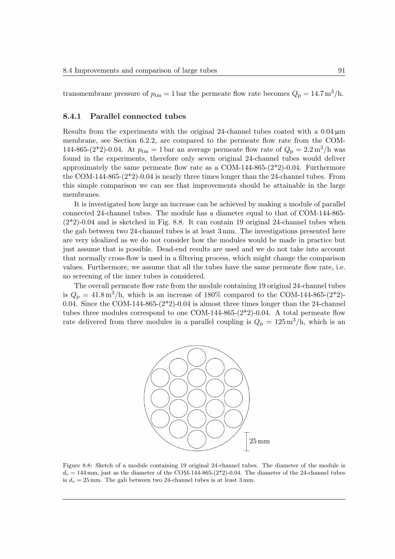
8.4 Improvements and comparison of large tubes 91
transmembrane pressure of ptm = 1 bar the permeate flow rate becomes Qp = 14.7m3/h.
8.4.1 Parallel connected tubes
Results from the experiments with the original 24-channel tubes coated with a 0.04 µmmembrane, see Section 6.2.2, are compared to the permeate flow rate from the COM-144-865-(2*2)-0.04. At ptm = 1 bar an average permeate flow rate of Qp = 2.2m3/h wasfound in the experiments, therefore only seven original 24-channel tubes would deliverapproximately the same permeate flow rate as a COM-144-865-(2*2)-0.04. Furthermorethe COM-144-865-(2*2)-0.04 is nearly three times longer than the 24-channel tubes. Fromthis simple comparison we can see that improvements should be attainable in the largemembranes.
It is investigated how large an increase can be achieved by making a module of parallelconnected 24-channel tubes. The module has a diameter equal to that of COM-144-865-(2*2)-0.04 and is sketched in Fig. 8.8. It can contain 19 original 24-channel tubes whenthe gab between two 24-channel tubes is at least 3 mm. The investigations presented hereare very idealized as we do not consider how the modules would be made in practice butjust assume that is possible. Dead-end results are used and we do not take into accountthat normally cross-flow is used in a filtering process, which might change the comparisonvalues. Furthermore, we assume that all the tubes have the same permeate flow rate, i.e.no screening of the inner tubes is considered.
The overall permeate flow rate from the module containing 19 original 24-channel tubesis Qp = 41.8m3/h, which is an increase of 180% compared to the COM-144-865-(2*2)-0.04. Since the COM-144-865-(2*2)-0.04 is almost three times longer than the 24-channeltubes three modules correspond to one COM-144-865-(2*2)-0.04. A total permeate flowrate delivered from three modules in a parallel coupling is Qp = 125 m3/h, which is an
25 mm
Figure 8.8: Sketch of a module containing 19 original 24-channel tubes. The diameter of the module isdo = 144 mm, just as the diameter of the COM-144-865-(2*2)-0.04. The diameter of the 24-channel tubesis do = 25mm. The gab between two 24-channel tubes is at least 3 mm.

92 CHAPTER 8. GEOMETRICAL OPTIMIZATION
increase of 750%. This is only a loose comparison, but it shows that significant increasesin the permeate flow rate can be achieved by parallel coupling small tubes compared tolarge standard tubes.
In Section 8.3 a new geometry, the 18-channel tube, was introduced and the EC simu-lations showed that an increase of approximately 37% could be achieved in the permeateflow rate with coated tubes compared to the EC simulations of the original 24-channeltube. Using the 18-channel tubes with a length of L = 305mm in a module would resultin a permeate flow rate of Qp = 38.6m3/h, which is an increase of 160% compared to theCOM-144-865-(2*2)-0.04. This a bit smaller than the flow rate from the module of orig-inal 24-channel tubes which is because the measured flow rates found in the experimentsare used in that module. In the simulations we assume that the membrane thickness onthe tubes is equal to that on the monotubes, and therefore the predicted flow rate fromthe 18-channel tubes is lower than the measured flow rate from the original 24-channeltubes. In practice a module of 18-channel tubes might have an even higher flow rate thanpredicted in these simulations.
If the hexagonal tubes with a length of L = 305mm are used 37 tubes can fit insidea module, still with a gab of minimum 3 mm, see Appendix D. The permeate flow ratefrom such a module would be Qp = 40.3m3/h and thus approximately the same as froma module of 18-channel tubes. The channels in the hexagonal tubes are very large witha hydraulic diameter of more than dh = 4.5mm, whereas the 18-channel tube has amaximum hydraulic diameter in the channels of dh = 3.7mm. If long tubes are neededthe hexagonal tubes would then be the preferable choice due to the low hydraulic resistancein the channels.
8.4.2 New design of a COM-144-865-(2*2)-0.04
The geometries presented in this section have only been implemented in the Comsolmodel as it would demand too much time to implement them in our EC model.
A Comsol simulation of one eighth of a COM-144-865-(2*2)-0.04 is made and thepressure distributions as well as the permeate flow rate results are shown in Fig. 8.9.The screening of the inner channels is obvious in this large tube making the majority ofthe channels inefficient, even when the 0.04 µm membrane is added. The flow rate foundin the 2D Comsol model of the COM-144-865-(2*2)-0.04 with the membrane added isQp = 30.0m3/h when it has a length of L = 865mm. The calculated flow rate is thentwice the flow rate stated by CoMeTas. Fig. 8.5(b) show that the EC model of the 60-channel tube, which is a smaller version of the COM-144-865-(2*2)-0.04, predicts roughlyhalf the permeate flow rate compared to the Comsol model at a length of L ≈ 850mmand this is assumed to be the same for the COM-144-865-(2*2)-0.04. It therefore seemslikely that the Comsol model predicts twice the flow rate.
12 cuts are made into the original geometry in order to reduce the screening of theinner channels. The geometry with the pressure distribution and the results from thesimulations in Comsol are shown in Fig. 8.10. The 12 cuts have a width of 4.8mm andtwo rows of channels have then been removed in each of the cuts. The increase in both thesurface area and the permeate flow rate is 280% compared to Comsol simulations of the

8.4 Improvements and comparison of large tubes 93
(a) (b)
0 bar
0.5 bar
1 bar
0 bar
0.5 bar
1 bar
(c)
Qp [m3/h]
Substrate 1300.04 µm membrane 30.0
(d)
A [m2]
Surface area 0.39Membrane area 14.3
20 mm 20 mm
Figure 8.9: Pressure distribution in a COM-144-865-(2*2)-0.04 with a diameter and length of do = 144mmand L = 865mm, respectively. The tube is a larger version of the 60-channel tube and therefore has wallthickness of w = 0.8mm and the size of the channels is 2mm × 2mm. (a) Substrate. (b) Coated with a0.04 µm membrane. (c) Permeate flow rate results. (d) Surface and membrane areas.
original geometry. This is a higher increase than seen with a module of parallel connectedtubes, but this large tube is nearly three times longer than the small tubes. Using threemodules of parallel connected small tubes would therefore be better. However, it might
(a) (b)
0 bar
0.5 bar
1 bar
0 bar
0.5 bar
1 bar
(c)
Qp [m3/h]
Substrate 5190.04 µm membrane 113
(d)
A [m2]
Surface area 1.50Membrane area 11.1
30 mm 30 mm
Figure 8.10: The pressure distribution of the COM-144-865-(2*2)-0.04 with 12 cuts. The cuts are 4.8mmwide, thus two rows of channels disappear, and the depth varies between the cuts. (a) Pure substrate. (b)Coated with a 0.04 µm membrane. (c) Permeate flow rate results. (d) Surface and membrane areas.
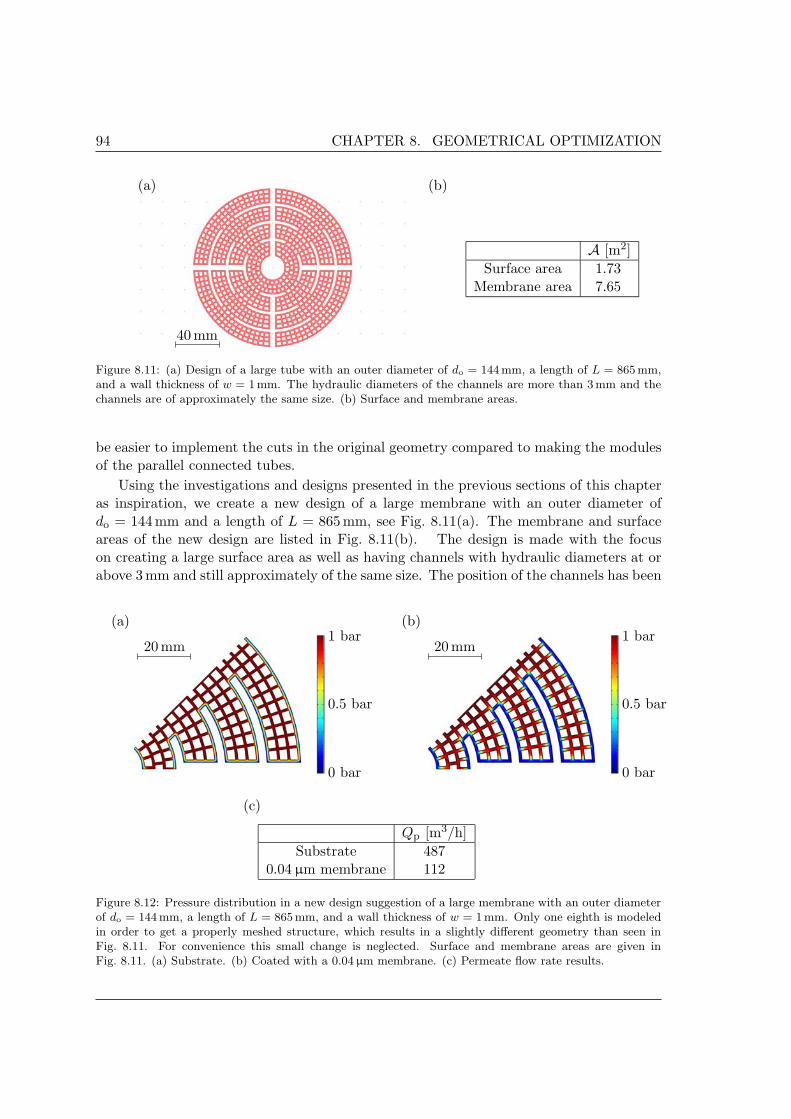
94 CHAPTER 8. GEOMETRICAL OPTIMIZATION
(a) (b)
A [m2]
Surface area 1.73Membrane area 7.65
40 mm
Figure 8.11: (a) Design of a large tube with an outer diameter of do = 144 mm, a length of L = 865 mm,and a wall thickness of w = 1mm. The hydraulic diameters of the channels are more than 3 mm and thechannels are of approximately the same size. (b) Surface and membrane areas.
be easier to implement the cuts in the original geometry compared to making the modulesof the parallel connected tubes.
Using the investigations and designs presented in the previous sections of this chapteras inspiration, we create a new design of a large membrane with an outer diameter ofdo = 144mm and a length of L = 865 mm, see Fig. 8.11(a). The membrane and surfaceareas of the new design are listed in Fig. 8.11(b). The design is made with the focuson creating a large surface area as well as having channels with hydraulic diameters at orabove 3 mm and still approximately of the same size. The position of the channels has been
(a) (b)
0 bar
0.5 bar
1 bar
0 bar
0.5 bar
1 bar
(c)
Qp [m3/h]
Substrate 4870.04 µm membrane 112
20 mm 20 mm
Figure 8.12: Pressure distribution in a new design suggestion of a large membrane with an outer diameterof do = 144 mm, a length of L = 865mm, and a wall thickness of w = 1mm. Only one eighth is modeledin order to get a properly meshed structure, which results in a slightly different geometry than seen inFig. 8.11. For convenience this small change is neglected. Surface and membrane areas are given inFig. 8.11. (a) Substrate. (b) Coated with a 0.04 µm membrane. (c) Permeate flow rate results.
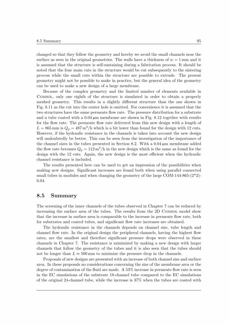
8.5 Summary 95
changed so that they follow the geometry and hereby we avoid the small channels near thesurface as seen in the original geometries. The walls have a thickness of w = 1 mm and itis assumed that the structure is self-sustaining during a fabrication process. It should benoted that the four main cuts in the structure would be cut subsequently to the sinteringprocess while the small cuts within the structure are possible to extrude. The presentgeometry might not be possible to make in practice, but the general idea of the geometrycan be used to make a new design of a large membrane.
Because of the complex geometry and the limited number of elements available inComsol, only one eighth of the structure is simulated in order to obtain a properlymeshed geometry. This results in a slightly different structure than the one shown inFig. 8.11 as the cut into the center hole is omitted. For convenience it is assumed that thetwo structures have the same permeate flow rate. The pressure distribution for a substrateand a tube coated with a 0.04 µm membrane are shown in Fig. 8.12 together with resultsfor the flow rate. The permeate flow rate delivered from this new design with a length ofL = 865 mm is Qp = 487 m3/h which is a bit lower than found for the design with 12 cuts.However, if the hydraulic resistance in the channels is taken into account the new designwill undoubtedly be better. This can be seen from the investigation of the importance ofthe channel sizes in the tubes presented in Section 8.2. With a 0.04 µm membrane addedthe flow rate becomes Qp = 112m3/h in the new design which is the same as found for thedesign with the 12 cuts. Again, the new design is the most efficient when the hydraulicchannel resistance is included.
The results presented here can be used to get an impression of the possibilities whenmaking new designs. Significant increases are found both when using parallel connectedsmall tubes in modules and when changing the geometry of the large COM-144-865-(2*2)-0.04.
8.5 Summary
The screening of the inner channels of the tubes observed in Chapter 7 can be reduced byincreasing the surface area of the tubes. The results from the 2D Comsol model showthat the increase in surface area is comparable to the increase in permeate flow rate, bothfor substrates and coated tubes, and significant flow rate increases are obtained.
The hydraulic resistance in the channels depends on channel size, tube length andchannel flow rate. In the original design the peripheral channels, having the highest flowrates, are the smallest and therefore significant pressure drops were observed in thesechannels in Chapter 7. The resistance is minimized by making a new design with largerchannels that follow the geometry of the tubes and it is also seen that the tubes shouldnot be longer than L ≈ 500mm to minimize the pressure drop in the channels.
Proposals of new designs are presented with an increase of both channel size and surfacearea. In these proposals no considerations concerning the size of the membrane area or thedegree of contamination of the fluid are made. A 53% increase in permeate flow rate is seenin the EC simulations of the substrate 18-channel tube compared to the EC simulationsof the original 24-channel tube, while the increase is 37% when the tubes are coated with
96 CHAPTER 8. GEOMETRICAL OPTIMIZATION
a 0.04µm membrane. The new design for the COM-144-865-(2*2)-0.04 tube increases thepermeate flow rate by 270% for both the uncoated and coated tube comparing to theoriginal COM-144-865-(2*2)-0.04 in the Comsol model and the increase might be evenlarger when including the hydraulic channel resistance.
Idealized modules with the same diameter as the COM-144-865-(2*2)-0.04 are madecontaining parallel connected tubes, and a module can contain 19 18-channel tubes. Whenthese tubes have a length of L = 305 mm, the permeate flow rate from such a module isapproximately 160% higher compared to data for the original COM-144-865-(2*2)-0.04,even though the COM-144-865-(2*2)-0.04 is almost three times longer. This is only a loosecomparison, but it shows that significant increases can be achieved by parallel couplingsmall tubes.
The new designs presented in this chapter show that higher flow rates are easily at-tainable and the efficiency of the tubes can be increased significantly.
Chapter 9
Conclusion and outlook
9.1 Conclusion
The work presented in this thesis can be categorized into experimental and numericalwork. The experimental work includes fabrication and flow measurements of various SiC-samples, while the numerical work includes validation of the two numerical models withthe experimental results and geometry optimization of the tubes regarding the permeatingflow. Only water is used in the experiments during this thesis and the filtration processitself is not investigated.
Experiments with plugs and monotubes show a linear relation between permeate flowrate and transmembrane pressure and we conclude that Darcy’s law is valid in porous SiC.The experiments with thin-walled and thick-walled monotubes show that the permeabilityis independent of the SiC thickness and it is found to be k = (8.3 ± 0.7) × 10−13 m2
for the substrate. For 24-channel tubes the relation between permeate flow rate andtransmembrane pressure is nonlinear. We find this to be due to a large hydraulic resistancein the channels of the tubes giving rise to a significant pressure drop down the length ofthe 24-channel tubes.
Simulations show that the peripheral channels screen the inner channels in the 24-channel tubes even when the tubes are coated with membranes and the efficiency of thetubes is therefore low. We have made different suggestions for optimized geometries re-garding the permeate flow rate focusing on three parameters, the length of the tubes, thesize of the channels and the surface area. Different suggestions are compared to an exist-ing membrane geometry used by CoMeTas and significant increases in the permeate flowrate are obtained. Making simple cuts in the surface of the tubes to increase the surfacearea can increase the permeate flow rate by roughly 50% in 24-channel tubes and morethan 250% in large membranes. More advanced optimization suggestions with modulesconsisting of many small tubes in parallel connection might increase the permeate flowrate even more compared to the existing large membrane.
Thin-walled monotubes and 24-channel tubes are coated with two different membranelayers, a 0.1µm membrane and a 0.04 µm membrane. It is expected that tubes coatedwith the 0.04µm membrane has the lowest flow rate, but it is found to be only slightly
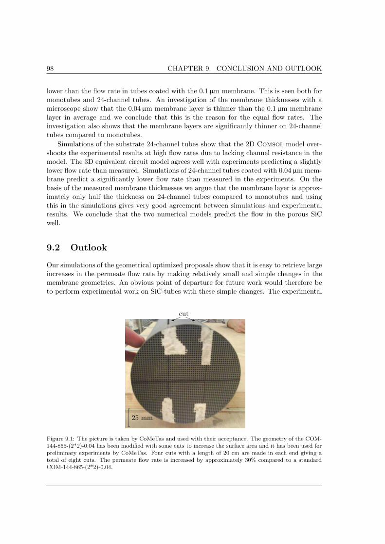
98 CHAPTER 9. CONCLUSION AND OUTLOOK
lower than the flow rate in tubes coated with the 0.1 µm membrane. This is seen both formonotubes and 24-channel tubes. An investigation of the membrane thicknesses with amicroscope show that the 0.04µm membrane layer is thinner than the 0.1µm membranelayer in average and we conclude that this is the reason for the equal flow rates. Theinvestigation also shows that the membrane layers are significantly thinner on 24-channeltubes compared to monotubes.
Simulations of the substrate 24-channel tubes show that the 2D Comsol model over-shoots the experimental results at high flow rates due to lacking channel resistance in themodel. The 3D equivalent circuit model agrees well with experiments predicting a slightlylower flow rate than measured. Simulations of 24-channel tubes coated with 0.04µm mem-brane predict a significantly lower flow rate than measured in the experiments. On thebasis of the measured membrane thicknesses we argue that the membrane layer is approx-imately only half the thickness on 24-channel tubes compared to monotubes and usingthis in the simulations gives very good agreement between simulations and experimentalresults. We conclude that the two numerical models predict the flow in the porous SiCwell.
9.2 Outlook
Our simulations of the geometrical optimized proposals show that it is easy to retrieve largeincreases in the permeate flow rate by making relatively small and simple changes in themembrane geometries. An obvious point of departure for future work would therefore beto perform experimental work on SiC-tubes with these simple changes. The experimental
25 mm
cut
Figure 9.1: The picture is taken by CoMeTas and used with their acceptance. The geometry of the COM-144-865-(2*2)-0.04 has been modified with some cuts to increase the surface area and it has been used forpreliminary experiments by CoMeTas. Four cuts with a length of 20 cm are made in each end giving atotal of eight cuts. The permeate flow rate is increased by approximately 30% compared to a standardCOM-144-865-(2*2)-0.04.
9.2 Outlook 99
work could also be extended to include some of the more complicated geometries we havesuggested, but this will of course encompass development and fabrication of the geometriesin question.
To be able to simulate the flow in the SiC-tubes better it would be beneficial to extendthe numerical model to include inlet and outlet effects on the tubes, a transition zone fromlaminar to turbulent flow in the channels, and inertia forces in the equations. In order tolook at the filtering process in the tubes, a new numerical model could also be developedthat includes particulate material in the flow. This way it would be possible to investigatethe dynamic filter cake on the surface of the membrane and it will be possible to checkhow this influences an optimization of the membrane geometry.
It would be very interesting to use topology optimization when looking at the opti-mization process of the membrane geometry. This method would make it easier and fasterto retrieve suggestions which could result in very efficient membranes and indicate sometendencies which could be used when designing new membranes.
CoMeTas has conducted a few preliminary experiments with a membrane using oneof the simple design proposal we have presented. They have increased the surface area oftheir COM-144-865-(2*2)-0.04 by making eight cuts with an angle grinder, see Fig. 9.1.The cuts increase the permeate flow rate by approximately 30% compared to the flow ratefrom a standard COM-144-865-(2*2)-0.04. These preliminary experiments demonstratethat significant increases in the permeate flow rate can be obtained. Furthermore the ex-periments verify that focusing on increasing the surface area is important when optimizingthe membranes.

100 CHAPTER 9. CONCLUSION AND OUTLOOK
Appendix A
Characterization methods
The simple methods that can be used to characterize the porous SiC by its porosity andpore size are shortly presented in the following.
A.1 Porosity
The porosity of the SiC used in our plugs and tubes, can be found from a simple experimentwith the thin-walled and thick-walled monotubes. The mass md of the dry monotubesis measured, and then the monotubes are immersed in demineralized water until theyare completely saturated with water. Afterwards, the mass ms of the now saturatedmonotubes is measured. The volume VSiC of the SiC in the monotubes is found as
VSiC = πL(d2
o
4− d2
c
4
), (A.1)
where L is the length, do is the outer diameter, and dc is the channel diameter of themonotubes. The volume Vw of the absorbed water can be estimated by subtracting themass of the dry monotubes from the mass of the saturated monotubes and dividing bythe density ρ = 1000 kg/m3 of the water,
Vw =ms −md
ρ. (A.2)
Hereafter the porosity φSiC of the SiC is calculated from the relation between Eqs. (A.1)and (A.2),
φSiC =Vw
VSiC. (A.3)
We used ten thin-walled and eight thick-walled monotubes for this porosity experiment.All of them had a length of L = 305mm and an outer diameter of do = 21.3mm, whilethe channel diameter was dc = 16.9mm for the thin-walled monotubes and dc = 14.1mmfor the thick-walled monotubes. The mean porosity, in %, of the SiC was found to be
φSiC = (38.2± 0.8)%, (A.4)
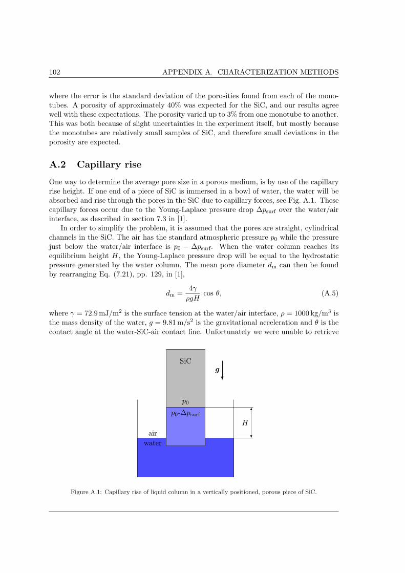
102 APPENDIX A. CHARACTERIZATION METHODS
where the error is the standard deviation of the porosities found from each of the mono-tubes. A porosity of approximately 40% was expected for the SiC, and our results agreewell with these expectations. The porosity varied up to 3% from one monotube to another.This was both because of slight uncertainties in the experiment itself, but mostly becausethe monotubes are relatively small samples of SiC, and therefore small deviations in theporosity are expected.
A.2 Capillary rise
One way to determine the average pore size in a porous medium, is by use of the capillaryrise height. If one end of a piece of SiC is immersed in a bowl of water, the water will beabsorbed and rise through the pores in the SiC due to capillary forces, see Fig. A.1. Thesecapillary forces occur due to the Young-Laplace pressure drop ∆psurf over the water/airinterface, as described in section 7.3 in [1].
In order to simplify the problem, it is assumed that the pores are straight, cylindricalchannels in the SiC. The air has the standard atmospheric pressure p0 while the pressurejust below the water/air interface is p0 − ∆psurf. When the water column reaches itsequilibrium height H, the Young-Laplace pressure drop will be equal to the hydrostaticpressure generated by the water column. The mean pore diameter dm can then be foundby rearranging Eq. (7.21), pp. 129, in [1],
dm =4γ
ρgHcos θ, (A.5)
where γ = 72.9mJ/m2 is the surface tension at the water/air interface, ρ = 1000 kg/m3 isthe mass density of the water, g = 9.81m/s2 is the gravitational acceleration and θ is thecontact angle at the water-SiC-air contact line. Unfortunately we were unable to retrieve
SiC
air
water
H
p0
p0-∆psurf
g
Figure A.1: Capillary rise of liquid column in a vertically positioned, porous piece of SiC.
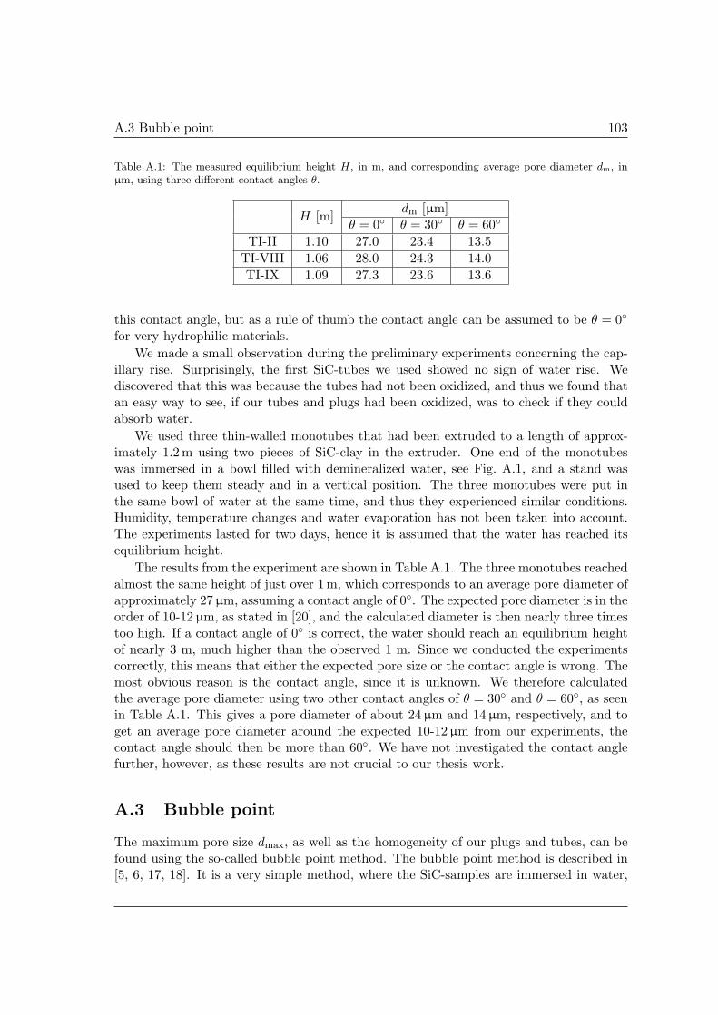
A.3 Bubble point 103
Table A.1: The measured equilibrium height H, in m, and corresponding average pore diameter dm, inµm, using three different contact angles θ.
H [m]dm [µm]
θ = 0 θ = 30 θ = 60
TI-II 1.10 27.0 23.4 13.5TI-VIII 1.06 28.0 24.3 14.0TI-IX 1.09 27.3 23.6 13.6
this contact angle, but as a rule of thumb the contact angle can be assumed to be θ = 0
for very hydrophilic materials.We made a small observation during the preliminary experiments concerning the cap-
illary rise. Surprisingly, the first SiC-tubes we used showed no sign of water rise. Wediscovered that this was because the tubes had not been oxidized, and thus we found thatan easy way to see, if our tubes and plugs had been oxidized, was to check if they couldabsorb water.
We used three thin-walled monotubes that had been extruded to a length of approx-imately 1.2m using two pieces of SiC-clay in the extruder. One end of the monotubeswas immersed in a bowl filled with demineralized water, see Fig. A.1, and a stand wasused to keep them steady and in a vertical position. The three monotubes were put inthe same bowl of water at the same time, and thus they experienced similar conditions.Humidity, temperature changes and water evaporation has not been taken into account.The experiments lasted for two days, hence it is assumed that the water has reached itsequilibrium height.
The results from the experiment are shown in Table A.1. The three monotubes reachedalmost the same height of just over 1 m, which corresponds to an average pore diameter ofapproximately 27µm, assuming a contact angle of 0. The expected pore diameter is in theorder of 10-12µm, as stated in [20], and the calculated diameter is then nearly three timestoo high. If a contact angle of 0 is correct, the water should reach an equilibrium heightof nearly 3 m, much higher than the observed 1 m. Since we conducted the experimentscorrectly, this means that either the expected pore size or the contact angle is wrong. Themost obvious reason is the contact angle, since it is unknown. We therefore calculatedthe average pore diameter using two other contact angles of θ = 30 and θ = 60, as seenin Table A.1. This gives a pore diameter of about 24µm and 14µm, respectively, and toget an average pore diameter around the expected 10-12µm from our experiments, thecontact angle should then be more than 60. We have not investigated the contact anglefurther, however, as these results are not crucial to our thesis work.
A.3 Bubble point
The maximum pore size dmax, as well as the homogeneity of our plugs and tubes, can befound using the so-called bubble point method. The bubble point method is described in[5, 6, 17, 18]. It is a very simple method, where the SiC-samples are immersed in water,

104 APPENDIX A. CHARACTERIZATION METHODS
and air pressure is then applied upstream, increasing it slowly until air bubbles are formedon the downstream surface, see Fig. A.2. This pressure is called the bubble point pressurepb, and it is defined as the pressure needed to press a steady stream of air bubbles throughthe largest pores in a saturated, porous medium, [17]. This means that we had to estimatewhen the bubble point pressure occurred by the amount of air bubbles coming throughthe porous SiC-samples. The bubble point test can be used not only for estimating themaximum pore diameter, but may also indicate if our plugs and tubes are damaged. Ifbubbles form at a lower pressure than expected, and only in one region of the SiC-sample,it could indicate a hole or a crack in the sample.
It is assumed that the pores are straight, circular channels, as in the capillary rise ex-periment, and the maximum pore size can be found from Eq. (A.6), which is a modificationof Eq. (A.5),
dmax =4γ
pbcos θ. (A.6)
As in Eq. (A.5) γ = 72.9mJ/m2 is the surface tension at the water/air interface and θ isthe contact angle at the water-SiC-air contact line.
Seven thin-walled and six thick-walled monotubes were used in the experiments. Theexperimental setup is shown in Fig. A.2. Pressurised air was connected to one end of themonotubes and the other end was sealed. The tubes were then immersed in demineralizedwater for at least ten minutes, until they were fully saturated. Afterwards the air pressurewas slowly increased until air bubbles formed on the outer surface of the monotubes, andthe bubble point pressure was observed. The experiment was repeated several times forall the monotubes, in order to check that the correct bubble point pressure had beenobtained.
The average bubble point pressure found for the 13 monotubes is listed in Table A.2,as well as the estimated maximum pore diameter at three different contact angles. Theerrors are the standard deviations of the pressures and pore diameters found from each ofthe monotubes. The average maximum pore diameter is 16.2µm, when a contact angle ofθ = 0 is assumed. As mentioned, the mean pore diameter is expected to be around 10-12µm, and it is expected that the maximum pore diameter is only slightly larger. Thus,
Water
Air
flow
Plastic tube
Seal
Monotube
Figure A.2: Experimental setup for the bubble point experiments showing the cross-section of a monotube.For clarity the dimensions have been altered on the sketch. The monotube is immersed in a bowl ofdemineralized water and air flow is supplied in one end, while the other end is sealed.
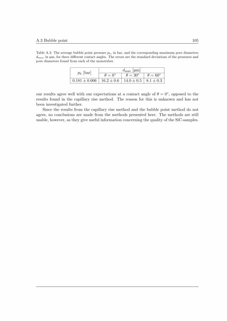
A.3 Bubble point 105
Table A.2: The average bubble point pressure pb, in bar, and the corresponding maximum pore diametersdmax, in µm, for three different contact angles. The errors are the standard deviations of the pressures andpore diameters found from each of the monotubes.
pb [bar]dmax [µm]
θ = 0 θ = 30 θ = 60
0.181± 0.006 16.2± 0.6 14.0± 0.5 8.1± 0.3
our results agree well with our expectations at a contact angle of θ = 0, opposed to theresults found in the capillary rise method. The reason for this is unknown and has notbeen investigated further.
Since the results from the capillary rise method and the bubble point method do notagree, no conclusions are made from the methods presented here. The methods are stillusable, however, as they give useful information concerning the quality of the SiC-samples.

106 APPENDIX A. CHARACTERIZATION METHODS

Appendix B
Investigation of the experimentalsetup
The pressure drops in the experimental setup between the initial position of the pressuretransmitters and the housing is investigated and calculated analytically. This check iscarried out to see if the pressure drops in the setup will have an influence on the measuredpressures. The pressure drops presented in this appendix will not be described in detailand only the results will be given.
The flow rate in the pipes on the setup is assumed to be between Q = 1 m3/h andQ = 4 m3/h during the experiments and the pipe diameters vary from D = 18 mm toD = 46mm. The Reynolds number, found from Eq. (2.2), then varies from Re = 7.5× 10³
to Re = 8× 10⁴ using water in the pipes with ρ = 1000 kg/m3 and η = 10−3 Pa s. As theReynolds numbers are larger than Re = 4× 10³ , the pipe flow is thus fully turbulent atall times.
The loss in mechanical energy in a pipe system with viscous flow is described by theenergy equation, see Eq. (2.23). The kinetic energy coefficient α can be assumed to beα = 1 for turbulent flow which therefore will be used in this investigation. The pipes inthe setup are assumed to be smooth.
Major Losses
The major head losses are found from Eq. (2.25) and arise due to pipe roughness. Thefriction factor f is given by the Blasius correlation, Eq. (2.30), and is valid for turbulentflow in smooth pipes with Re ≤ 105 , see section 8-7 in [3].
Minor Losses
The minor losses are caused by a variety of fittings, bends and abrupt changes in diameterin the pipes and can be found from
hlm = KlV 2
2, (B.1a)
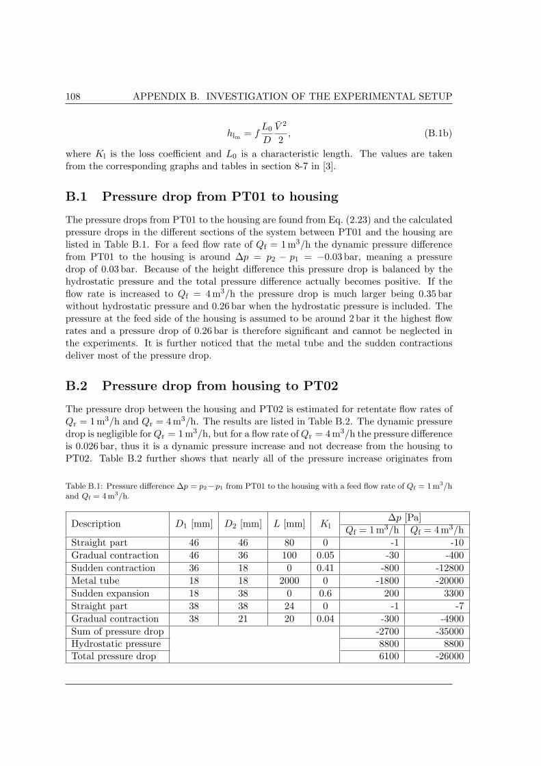
108 APPENDIX B. INVESTIGATION OF THE EXPERIMENTAL SETUP
hlm = fL0
D
V 2
2, (B.1b)
where Kl is the loss coefficient and L0 is a characteristic length. The values are takenfrom the corresponding graphs and tables in section 8-7 in [3].
B.1 Pressure drop from PT01 to housing
The pressure drops from PT01 to the housing are found from Eq. (2.23) and the calculatedpressure drops in the different sections of the system between PT01 and the housing arelisted in Table B.1. For a feed flow rate of Qf = 1m3/h the dynamic pressure differencefrom PT01 to the housing is around ∆p = p2 − p1 = −0.03 bar, meaning a pressuredrop of 0.03 bar. Because of the height difference this pressure drop is balanced by thehydrostatic pressure and the total pressure difference actually becomes positive. If theflow rate is increased to Qf = 4 m3/h the pressure drop is much larger being 0.35 barwithout hydrostatic pressure and 0.26 bar when the hydrostatic pressure is included. Thepressure at the feed side of the housing is assumed to be around 2 bar it the highest flowrates and a pressure drop of 0.26 bar is therefore significant and cannot be neglected inthe experiments. It is further noticed that the metal tube and the sudden contractionsdeliver most of the pressure drop.
B.2 Pressure drop from housing to PT02
The pressure drop between the housing and PT02 is estimated for retentate flow rates ofQr = 1 m3/h and Qr = 4 m3/h. The results are listed in Table B.2. The dynamic pressuredrop is negligible for Qr = 1 m3/h, but for a flow rate of Qr = 4m3/h the pressure differenceis 0.026 bar, thus it is a dynamic pressure increase and not decrease from the housing toPT02. Table B.2 further shows that nearly all of the pressure increase originates from
Table B.1: Pressure difference ∆p = p2−p1 from PT01 to the housing with a feed flow rate of Qf = 1 m3/hand Qf = 4 m3/h.
Description D1 [mm] D2 [mm] L [mm] Kl∆p [Pa]
Qf = 1 m3/h Qf = 4 m3/hStraight part 46 46 80 0 -1 -10Gradual contraction 46 36 100 0.05 -30 -400Sudden contraction 36 18 0 0.41 -800 -12800Metal tube 18 18 2000 0 -1800 -20000Sudden expansion 18 38 0 0.6 200 3300Straight part 38 38 24 0 -1 -7Gradual contraction 38 21 20 0.04 -300 -4900Sum of pressure drop -2700 -35000Hydrostatic pressure 8800 8800Total pressure drop 6100 -26000
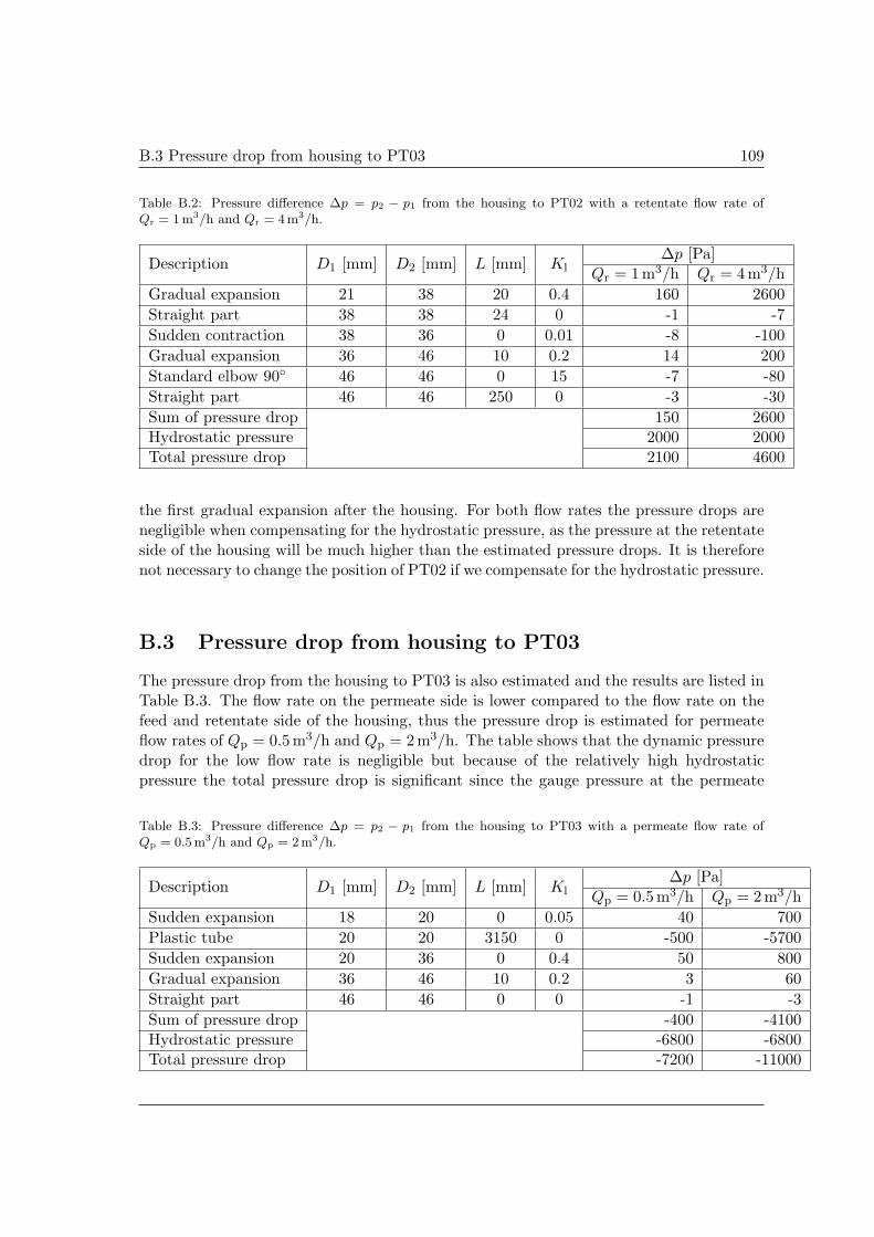
B.3 Pressure drop from housing to PT03 109
Table B.2: Pressure difference ∆p = p2 − p1 from the housing to PT02 with a retentate flow rate ofQr = 1m3/h and Qr = 4 m3/h.
Description D1 [mm] D2 [mm] L [mm] Kl∆p [Pa]
Qr = 1 m3/h Qr = 4 m3/hGradual expansion 21 38 20 0.4 160 2600Straight part 38 38 24 0 -1 -7Sudden contraction 38 36 0 0.01 -8 -100Gradual expansion 36 46 10 0.2 14 200Standard elbow 90 46 46 0 15 -7 -80Straight part 46 46 250 0 -3 -30Sum of pressure drop 150 2600Hydrostatic pressure 2000 2000Total pressure drop 2100 4600
the first gradual expansion after the housing. For both flow rates the pressure drops arenegligible when compensating for the hydrostatic pressure, as the pressure at the retentateside of the housing will be much higher than the estimated pressure drops. It is thereforenot necessary to change the position of PT02 if we compensate for the hydrostatic pressure.
B.3 Pressure drop from housing to PT03
The pressure drop from the housing to PT03 is also estimated and the results are listed inTable B.3. The flow rate on the permeate side is lower compared to the flow rate on thefeed and retentate side of the housing, thus the pressure drop is estimated for permeateflow rates of Qp = 0.5 m3/h and Qp = 2 m3/h. The table shows that the dynamic pressuredrop for the low flow rate is negligible but because of the relatively high hydrostaticpressure the total pressure drop is significant since the gauge pressure at the permeate
Table B.3: Pressure difference ∆p = p2 − p1 from the housing to PT03 with a permeate flow rate ofQp = 0.5m3/h and Qp = 2m3/h.
Description D1 [mm] D2 [mm] L [mm] Kl∆p [Pa]
Qp = 0.5m3/h Qp = 2 m3/hSudden expansion 18 20 0 0.05 40 700Plastic tube 20 20 3150 0 -500 -5700Sudden expansion 20 36 0 0.4 50 800Gradual expansion 36 46 10 0.2 3 60Straight part 46 46 0 0 -1 -3Sum of pressure drop -400 -4100Hydrostatic pressure -6800 -6800Total pressure drop -7200 -11000
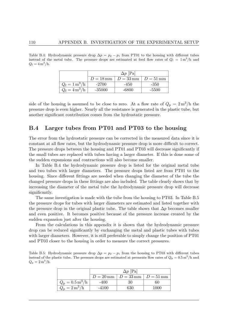
110 APPENDIX B. INVESTIGATION OF THE EXPERIMENTAL SETUP
Table B.4: Hydrodynamic pressure drop ∆p = p2 − p1 from PT01 to the housing with different tubesinstead of the metal tube. The pressure drops are estimated at feed flow rates of Qf = 1m3/h andQf = 4m3/h.
∆p [Pa]D = 18 mm D = 33mm D = 51 mm
Qf = 1m3/h -2700 -450 -350Qf = 4m3/h -35000 -6800 -5500
side of the housing is assumed to be close to zero. At a flow rate of Qp = 2 m3/h thepressure drop is even higher. Nearly all the resistance is generated in the plastic tube, butanother significant contribution comes from the hydrostatic pressure.
B.4 Larger tubes from PT01 and PT03 to the housing
The error from the hydrostatic pressure can be corrected in the measured data since it isconstant at all flow rates, but the hydrodynamic pressure drop is more difficult to correct.The pressure drops between the housing and PT01 and PT03 will decrease significantly ifthe small tubes are replaced with tubes having a larger diameter. If this is done some ofthe sudden expansions and contractions will also become smaller.
In Table B.4 the hydrodynamic pressure drop is listed for the original metal tubeand two tubes with larger diameters. The pressure drops listed are from PT01 to thehousing. Since different fittings are needed when changing the diameter of the tube thechanged pressure drops in these fittings are also included. The table clearly shows that byincreasing the diameter of the metal tube the hydrodynamic pressure drop will decreasesignificantly.
The same investigation is made with the tube from the housing to PT03. In Table B.5the pressure drops for tubes with larger diameters are estimated and listed together withthe pressure drop in the original plastic tube. The table shows that ∆p becomes smallerand even positive. It becomes positive because of the pressure increase created by thesudden expansion just after the housing.
From the calculations in this appendix it is shown that the hydrodynamic pressuredrop can be reduced significantly by exchanging the metal and plastic tubes with tubeswith larger diameters. However, it is still preferable to simply change the position of PT01and PT03 closer to the housing in order to measure the correct pressures.
Table B.5: Hydrodynamic pressure drop ∆p = p2 − p1 from the housing to PT03 with different tubesinstead of the plastic tube. The pressure drops are estimated at permeate flow rates of Qp = 0.5m3/h andQp = 2 m3/h.
∆p [Pa]D = 20 mm D = 33mm D = 51 mm
Qp = 0.5m3/h -400 30 60Qp = 2 m3/h -4100 630 1000
Appendix C
Additional experiments
Some additional experiments have been carried out and these will shortly be presented inthe following. A few cross-flow experiments have been conducted with both thin-walledmonotubes and 24-channel tubes to see how an increasing retentate flow rate influences therelation between permeate flow rate and transmembrane pressure. Furthermore experi-ments have been conducted with two 1m long thin-walled monotubes and with thin-walledmonotubes and 24-channel tubes coated with the 1µm membrane to see how this mem-brane influences the permeate flow rate.
C.1 Cross-flow experiments
Cross-flow measurements are carried out with different retentate flow rates in order toobserve the possible changes in the relation between the permeate flow rate Qp and thetransmembrane pressure ptm compared to dead-end experiments. The results from thecross-flow experiments carried out with monotube TI-XVIII-I and 24-channel tube XXIV-XIV coated with a 0.04µm membrane are included here and these results are representativefor the tendencies seen in the cross-flow experiments.
C.1.1 Monotubes
Fig. C.1 shows the results from both dead-end and cross-flow experiments with monotubeTI-XVIII-I. The cross-flow experiments are carried out at three different relative retentateflow rates compared to the feed flow rates. Qr/Qf changes slightly as the pressure isincreased and the values used here are calculated at the highest flow rates used. At lowretentate flow Qr/Qf = 35%, medium retentate flow Qr/Qf = 46% and high retentate flowQr/Qf = 60%. From Fig. C.1(a) it is seen that the relation between permeate flow rateand transmembrane pressure is unchanged even at the highest retentate flow rate used.This is also seen from Fig. C.1(b) where the constants for the best-fitted lines are listedfor the four different experiments. The slope a2 of the best-fitted lines are equal for allfour experiments. The reason that the Qp-ptm relation is unchanged is that the hydraulicresistance is negligible in the monotubes and the pressure distribution in the channel ofthe monotubes is therefore well estimated by the used equation for ptm, see Eq. (2.22).
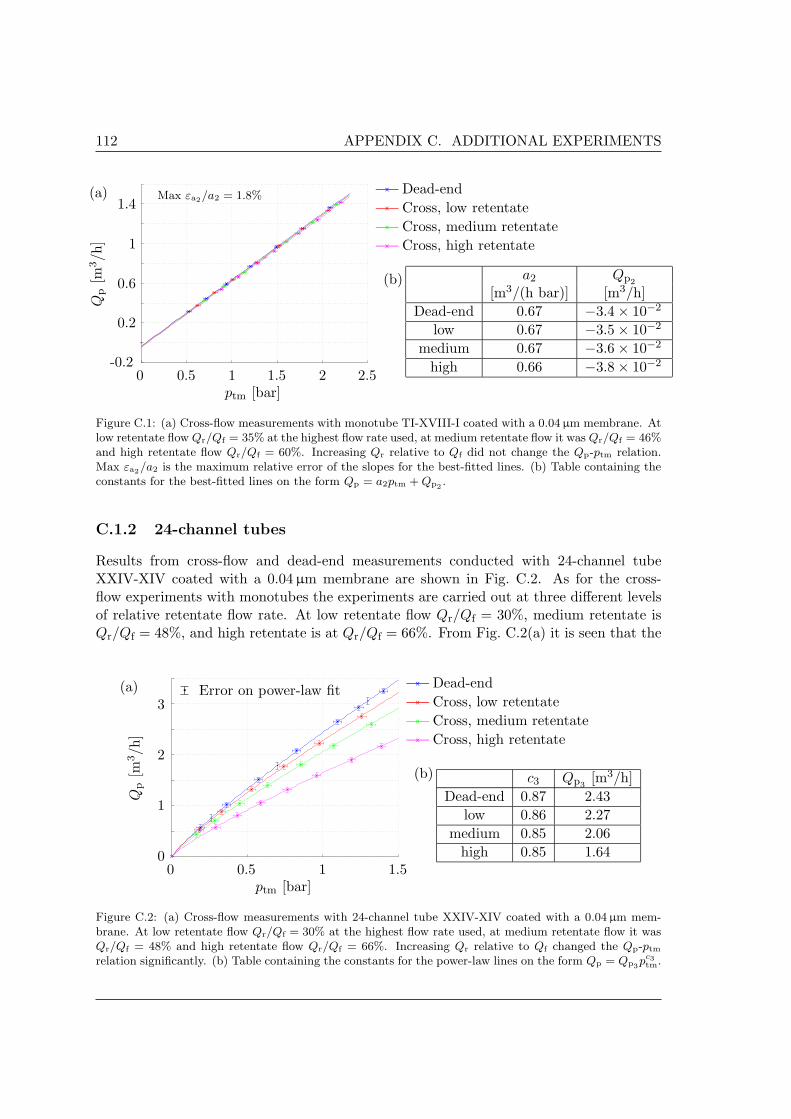
112 APPENDIX C. ADDITIONAL EXPERIMENTS
(a)
-0.2
0.2
0.6
1
1.4
0 0.5 1 1.5 2 2.5
Qp
[m3/h
]
ptm [bar]
x Dead-endx Cross, low retentatex Cross, medium retentatex Cross, high retentate
a2 Qp2
[m3/(h bar)] [m3/h]
Dead-end 0.67 −3.4 × 10⁻²
low 0.67 −3.5 × 10⁻²
medium 0.67 −3.6 × 10⁻²
high 0.66 −3.8 × 10⁻²
(b)
Max εa2/a2 = 1.8%
Figure C.1: (a) Cross-flow measurements with monotube TI-XVIII-I coated with a 0.04 µm membrane. Atlow retentate flow Qr/Qf = 35% at the highest flow rate used, at medium retentate flow it was Qr/Qf = 46%and high retentate flow Qr/Qf = 60%. Increasing Qr relative to Qf did not change the Qp-ptm relation.Max εa2/a2 is the maximum relative error of the slopes for the best-fitted lines. (b) Table containing theconstants for the best-fitted lines on the form Qp = a2ptm + Qp2 .
C.1.2 24-channel tubes
Results from cross-flow and dead-end measurements conducted with 24-channel tubeXXIV-XIV coated with a 0.04µm membrane are shown in Fig. C.2. As for the cross-flow experiments with monotubes the experiments are carried out at three different levelsof relative retentate flow rate. At low retentate flow Qr/Qf = 30%, medium retentate isQr/Qf = 48%, and high retentate is at Qr/Qf = 66%. From Fig. C.2(a) it is seen that the
(a)
0
1
2
3
0 0.5 1 1.5
Qp
[m3/h
]
ptm [bar]
x Dead-endx Cross, low retentatex Cross, medium retentatex Cross, high retentate
c3 Qp3[m3/h]
Dead-end 0.87 2.43
low 0.86 2.27
medium 0.85 2.06
high 0.85 1.64
(b)
· Error on power-law fit
Figure C.2: (a) Cross-flow measurements with 24-channel tube XXIV-XIV coated with a 0.04 µm mem-brane. At low retentate flow Qr/Qf = 30% at the highest flow rate used, at medium retentate flow it wasQr/Qf = 48% and high retentate flow Qr/Qf = 66%. Increasing Qr relative to Qf changed the Qp-ptm
relation significantly. (b) Table containing the constants for the power-law lines on the form Qp = Qp3pc3tm.

C.2 Long thin-walled monotube 113
Qp-ptm relation decreases significantly as Qr/Qf is increased. The constants for the power-law fitted lines are listed in Fig. C.2(b). These show that the power c3 does not changeas the retentate flow is increased but Qp3
decreases significantly. The permeate flow ratedecreases due to an increasing hydraulic resistance in the channels of the 24-channel tube,leading to a large pressure drop throughout the channels. As the flow is turbulent in thechannels the assumptions used for calculating ptm, see Section 2.2.4, are poor and ptm isthus not correct. This is the reason for the decreasing Qp-ptm relation.
C.2 Long thin-walled monotube
When the experiments with the 1m long thin-walled monotubes were conducted, a longhousing had to be used. It was not possible to mount PT03 at this housing, whichintroduced some problems when measuring the permeate pressure. The housing had twopermeate exits, one in each end, and therefore the permeate pressure could be measured ateither of them while the permeate water could be let out through one or both of them. Inorder to check how this influenced the measured permeate pressure both PT02 and PT03,mounted at the extra pipe part and the small housing, respectively, was used to measurethe pressure at the two exits, while the permeate water was let out through either or bothof them. Four measurements conducted with TI-XXI, where the permeate pressure wasmeasured in different ways, are shown in Fig. C.3. As the figure shows, the repeatability ispoor which is due to the permeate pressure not being measured properly. If the water waslet out through the same exit where the pressure was measured, a significant hydrodynamicpressure difference was introduced. If only one exit was used for the permeate water
0
4
8
12
0 0.4 0.8 1.2 1.6
Qp
[m3/h
]
ptm [bar]
x Nr 1x Nr 2x Nr 3x Nr 4
Qp = a1ptm
Qp = a2ptm + Qp2
Qp = Qp3
(
ptm
1 bar
)
c3
a1 = 6.3 m3/(h bar)
a2 = 5.6 m3/(h bar)
Qp2= 0.79 m3/h
c3 = 0.87
Qp3= 6.5 m3/h
εa2/a2 = 2.4%
Figure C.3: A plot of the measurements for the 1 m long, thin-walled monotube TI-XXI. Qp and ptm arenot linearly related due to a large hydraulic channel resistance in the long monotube. The error on themeasurements is significantly larger than in the experiments with the short monotubes because it was notpossible to measure the permeate pressure pp properly.

114 APPENDIX C. ADDITIONAL EXPERIMENTS
and the other was used to measure pp, the housing itself became restricting making themonotube less efficient. These problems were all dependent of the flow rate and thereforethey became more and more significant as the flow rate increased, as seen in Fig. C.3. Inthe end it was concluded that it was not possible to measure the true permeate pressureat high flow rates.
Fig. C.3 also shows another interesting aspect, namely that the permeate flow rate andthe transmembrane pressure are not linearly related for the long thin-walled monotubes.The best linear fit intersects with the Qp-axis in Qp2
= 0.79m3/h and the slopes of thebest fit and the linear line through (0, 0) are not equal. Also the power in the power-lawfit is c3 = 0.87 which clearly indicates that the relation is nonlinear.
This nonlinearity is not only because of the problems with measuring pp, but alsobecause at the high flow rates, the hydraulic channel resistance in the monotube becomessignificant. A pressure drop of nearly 0.2 bar was measured down the length of the mono-tube at a flow rate of 9 m3/h. Hence, by increasing the length of the tube, the hydraulicchannel resistance has increased considerably compared to the short monotubes whichresults in a nonlinear Qp-ptm profile.
C.3 Experiments with 1 µm membrane
Results from the experiments carried out with four short monotubes and four 24-channeltubes coated with a 1µm membrane are presented here. These experiments were con-ducted in order to investigate how the 1µm membrane effected the permeate flow rate.
C.3.1 Monotubes
The results from four short monotubes coated with a 1µm membrane are shown in Fig. C.4.A linear relation between the flow rate and the transmembrane pressure is seen for all thetubes. By comparing these results with the results from the uncoated, short monotubesa 15% decrease is seen in permeate flow rate. A decrease of 15% is not much and wecan conclude that adding the 1µm membrane to the tubes does not change the flow ratesignificantly. The spread between the slopes of the best-fitted lines is 10% indicating thatthe monotubes are uniformly coated with the 1µm membrane layer.
C.3.2 24-channel tubes
Experiments were conducted with four 24-channel tubes coated with the 1µm membrane,and the results from these measurements are seen in Fig. C.5. From this figure it isseen that the relation between the permeate flow rate and the transmembrane pressureis still nonlinear as seen in the substrate experiments. A decrease of approximately 20%in average is observed in the permeate flow rate when compared to the results from thesubstrate experiments. The spread on the flow rates is approximately 25% which is morethen seen for the monotubes having a spread of only 10%. This could indicate that the24-channel tubes have not been uniformly coated with the 1µm membrane.
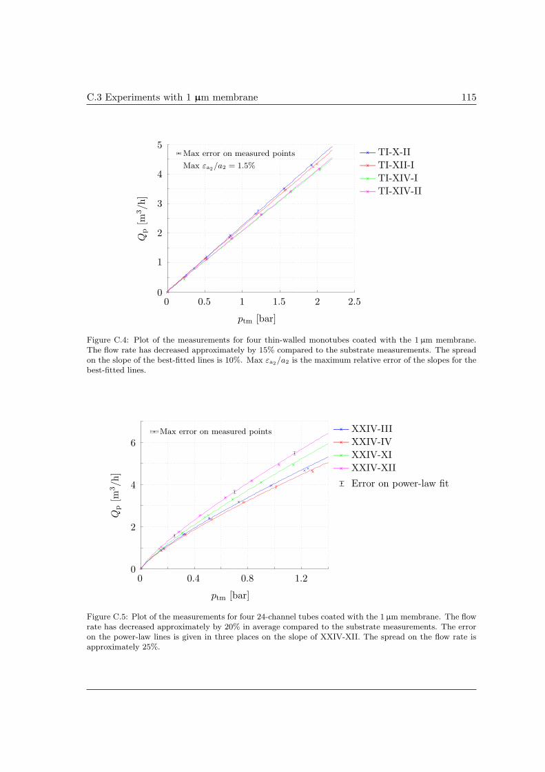
C.3 Experiments with 1 µm membrane 115
0
1
2
3
4
5
0 0.5 1 1.5 2 2.5
Qp
[m3/h
]
ptm [bar]
x TI-X-IIx TI-XII-Ix TI-XIV-Ix TI-XIV-II
Max error on measured points
Max εa2/a2 = 1.5%
Figure C.4: Plot of the measurements for four thin-walled monotubes coated with the 1 µm membrane.The flow rate has decreased approximately by 15% compared to the substrate measurements. The spreadon the slope of the best-fitted lines is 10%. Max εa2/a2 is the maximum relative error of the slopes for thebest-fitted lines.
0
2
4
6
0 0.4 0.8 1.2
Qp
[m3/h
]
ptm [bar]
x XXIV-IIIx XXIV-IVx XXIV-XIx XXIV-XII
Max error on measured points
· Error on power-law fit
Figure C.5: Plot of the measurements for four 24-channel tubes coated with the 1 µm membrane. The flowrate has decreased approximately by 20% in average compared to the substrate measurements. The erroron the power-law lines is given in three places on the slope of XXIV-XII. The spread on the flow rate isapproximately 25%.

116 APPENDIX C. ADDITIONAL EXPERIMENTS
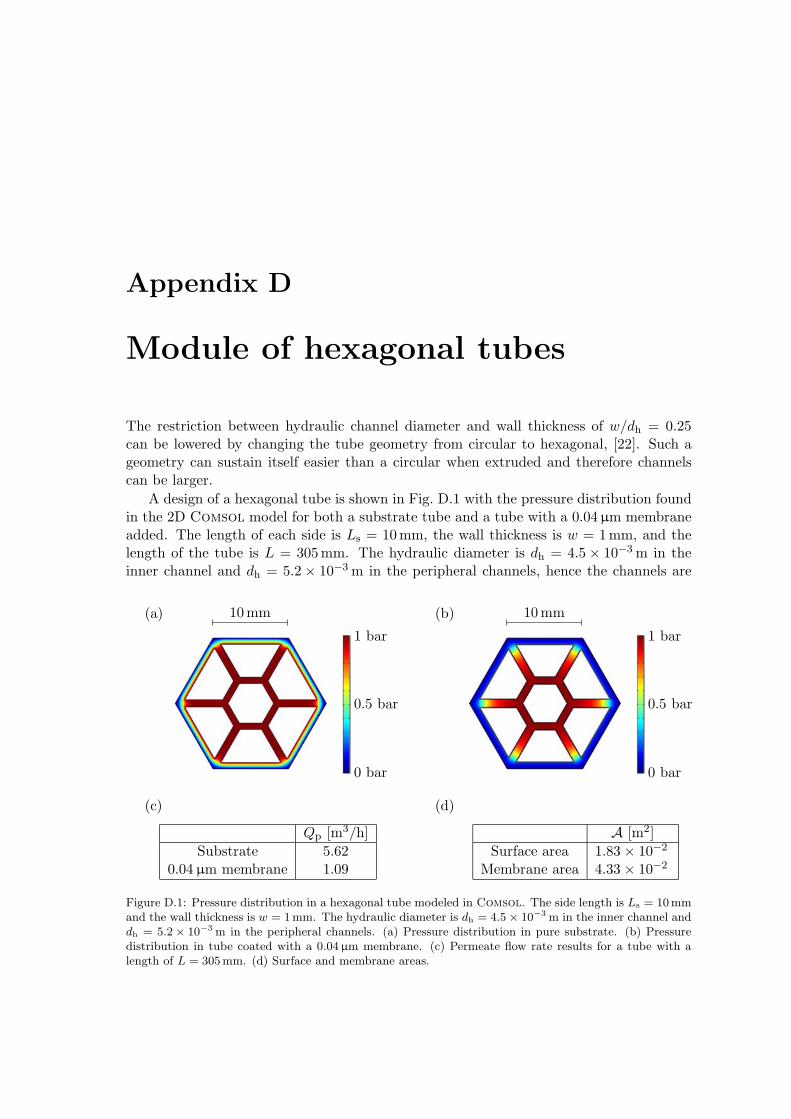
Appendix D
Module of hexagonal tubes
The restriction between hydraulic channel diameter and wall thickness of w/dh = 0.25can be lowered by changing the tube geometry from circular to hexagonal, [22]. Such ageometry can sustain itself easier than a circular when extruded and therefore channelscan be larger.
A design of a hexagonal tube is shown in Fig. D.1 with the pressure distribution foundin the 2D Comsol model for both a substrate tube and a tube with a 0.04 µm membraneadded. The length of each side is Ls = 10 mm, the wall thickness is w = 1 mm, and thelength of the tube is L = 305 mm. The hydraulic diameter is dh = 4.5× 10⁻³ m in theinner channel and dh = 5.2× 10⁻³ m in the peripheral channels, hence the channels are
(a) (b)
0 bar
0.5 bar
1 bar
0 bar
0.5 bar
1 bar
(c)
Qp [m3/h]
Substrate 5.620.04 µm membrane 1.09
(d)
A [m2]
Surface area 1.83 × 10⁻²
Membrane area 4.33 × 10⁻²
10 mm10 mm
Figure D.1: Pressure distribution in a hexagonal tube modeled in Comsol. The side length is Ls = 10 mmand the wall thickness is w = 1 mm. The hydraulic diameter is dh = 4.5× 10⁻³ m in the inner channel anddh = 5.2× 10⁻³ m in the peripheral channels. (a) Pressure distribution in pure substrate. (b) Pressuredistribution in tube coated with a 0.04 µm membrane. (c) Permeate flow rate results for a tube with alength of L = 305 mm. (d) Surface and membrane areas.
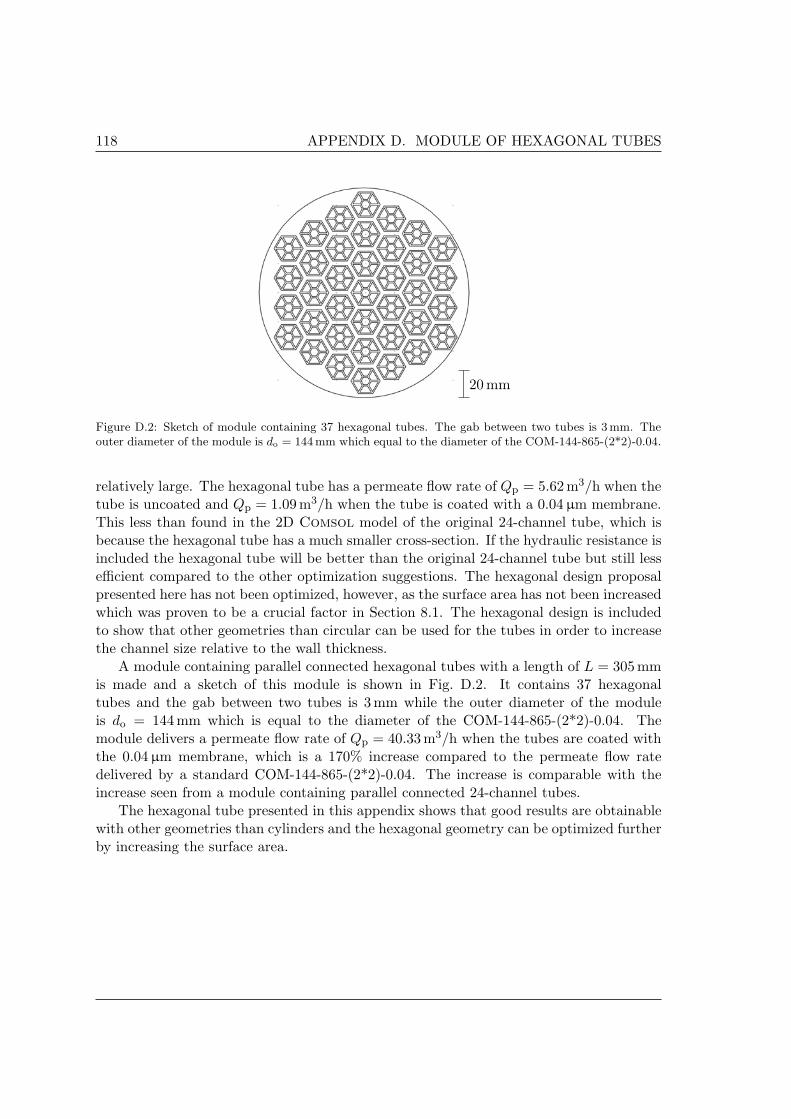
118 APPENDIX D. MODULE OF HEXAGONAL TUBES
20 mm
Figure D.2: Sketch of module containing 37 hexagonal tubes. The gab between two tubes is 3mm. Theouter diameter of the module is do = 144mm which equal to the diameter of the COM-144-865-(2*2)-0.04.
relatively large. The hexagonal tube has a permeate flow rate of Qp = 5.62m3/h when thetube is uncoated and Qp = 1.09m3/h when the tube is coated with a 0.04µm membrane.This less than found in the 2D Comsol model of the original 24-channel tube, which isbecause the hexagonal tube has a much smaller cross-section. If the hydraulic resistance isincluded the hexagonal tube will be better than the original 24-channel tube but still lessefficient compared to the other optimization suggestions. The hexagonal design proposalpresented here has not been optimized, however, as the surface area has not been increasedwhich was proven to be a crucial factor in Section 8.1. The hexagonal design is includedto show that other geometries than circular can be used for the tubes in order to increasethe channel size relative to the wall thickness.
A module containing parallel connected hexagonal tubes with a length of L = 305mmis made and a sketch of this module is shown in Fig. D.2. It contains 37 hexagonaltubes and the gab between two tubes is 3 mm while the outer diameter of the moduleis do = 144 mm which is equal to the diameter of the COM-144-865-(2*2)-0.04. Themodule delivers a permeate flow rate of Qp = 40.33m3/h when the tubes are coated withthe 0.04µm membrane, which is a 170% increase compared to the permeate flow ratedelivered by a standard COM-144-865-(2*2)-0.04. The increase is comparable with theincrease seen from a module containing parallel connected 24-channel tubes.
The hexagonal tube presented in this appendix shows that good results are obtainablewith other geometries than cylinders and the hexagonal geometry can be optimized furtherby increasing the surface area.

Appendix E
Data sheet
An official data sheet containing information about some of CoMeTas’ large standardmembranes is presented here. The information for the COM-144-865-(2*2)-0.04 having alength of L = 865mm, an outer diameter of do = 144 mm, a wall thickness of w = 0.8mm,containing approximately 1900 channels with a size of 2mm× 2mm and coated with the0.04 µm membrane is used for comparison to the optimization suggestions presented inChapter 8.

120 APPENDIX E. DATA SHEET

Appendix F
Working drawings
The working drawings included here have been created to improve the extruder head usedto produce the monotubes. The part with the new adjustment screws for the extruder headis shown in Appendix F.1, while the new inner cylinders for fabricating the thick-walledand thin-walled monotubes are shown in Appendixes F.2 and F.3, respectively.

122 APPENDIX F. WORKING DRAWINGS
F.1 Part for extruder head
Figure F.1: New part for the extruder head with holes for adjustment screws.

F.2 Thin inner cylinder 123
F.2 Thin inner cylinder
Figure F.2: Thin inner cylinder made out of brass used to make the thick-walled monotubes.

124 APPENDIX F. WORKING DRAWINGS
F.3 Thick inner cylinder
Figure F.3: Thick inner cylinder made out of brass used to make the thin-walled monotubes.

Bibliography
[1] Theoretical MicrofluidicsHenrik Bruus,Oxford University Press Inc, Oxford, GB, (2008).
[2] Dynamics of fluids in porous mediaJacob Bear,American Elsevier Publishing Company, New York, (1972).
[3] Introduction to fluid mechanicsRobert W. Fox, Alan T. McDonald and Philip J. Pritchard,John Wiley & sons Inc, International Edition, (2004).
[4] Viscous fluid flowFrank M. White,McGraw-Hill, Singapore, International Edition, (2006).
[5] Membrane Filtration - and related molecular separation technologiesEdited by: Werner Kofod Nielsen,APV Systems, (2000).
[6] Membrane Filtration - The Technology of Pressure-driven Crossflow ProcessesR. G. Gutman,Adam Hilger, Bristol, (1987).
[7] Flow Through Porous MediaRoger J. M. De Wiest,Academic press Inc, London, (1969).
[8] Flow in Porous Media with Special Reference to Breakwater StructuresOle Holst Andersen,Centertrykkeriet, Aalborg University, (1994).
[9] Introduction to Modeling of Transport Phenomena in Porous MediaJacob Bear and Yehuda Bachmat,Kluwer Academic Publichers, Dordrecht, (1990)

126 BIBLIOGRAPHY
[10] Thomas Eilkær Hansen,Flow in micro porous silicon carbideM.Sc. thesis, Department of Micro- and Nanotechnology, Technical University ofDenmark, (2007),http://www.nanotech.dtu.dk/Research/Theory/TMF/publications/MSc theses.aspx
[11] Brooks, C. S., Decrascente, M. A. and Scola, D. A.,The Wetting of Silicon Carbide SurfacesUnited Aircraft Research Laboratories. East Hartford, (1968).
[12] Fand, R. M., Kim, B. Y. K., Lam, A. C. C., and Phan, R. T.,Resistance to the Flow of Fluids Through Simple and Complex Porous Media WhoseMatrices Are Composed of Randomly Packed SpheresASME J. Fluids Eng., vol. 109, pp. 268-274, (1987).
[13] Ifiyenia Kececioglu and Yuxiang Jiang,Flow Through Porous Media of Packed Spheres Saturated With WaterASME J. Fluids Eng., vol. 116, pp. 164-170, (1994).
[14] Kagramanov, G. G., Dytnerskii, Yu. I. and Il’ib, P. G.,A model simulation of the filteringprocess in multichannel ceramic membranesVol. 42, Nos. 3-4, (2001)
[15] Alexopoulos, S., Breitbach, G., Hoffschmidt, B., Stobbe, P.,Computational fluid flow of porous ReSIC ceramic filtering modules and optimizationof the channel edge form geometry10th World Filtration Congress
[16] Schwartzendruber, Dale,Non-Darcy Flow Behaviour in Liquid-Saturated Porous Media Journal of Geophysi-cal Research, vol. 67, no. 13, (1962)
[17] ASTM F316-03,Standard Test Methods for Pore Size Characteristics of Membrane Filters by Bub-ble Point and Mean Flow Pore Test Annual book of ASTM standards. Section 11,volume 11.02, Water and Environmental Technology, (2007).
[18] ASTM E128-99,Standard Test Method for Maximum Pore Diameter and Permeability of RigidPorous Filters for Laboratory Use Annual book of ASTM standards. Section 14,General Methods and Instrumentation, (2005).
[19] Webpage of CoMeTas A/S:http://www.cometas.dk
[20] Webpage of LiqTech A/S:http://www.liqtech.dk

BIBLIOGRAPHY 127
[21] Webpage of DTI Oil and gas:http://ior.senergyltd.com/issue8/tp/
[22] Private communicationJohnny MarkerTechnical DirectorResearch & DevelopmentLiqTech A/Se-mail: [email protected]