this page intentionally left blank - mobt3ath.com · an introduction to the standard model of...
TRANSCRIPT


This page intentionally left blank

AN INTRODUCTION TO THE STANDARD MODEL OFPARTICLE PHYSICS
Second Edition
The Standard Model of particle physics is the mathematical theory that describesthe weak, electromagnetic and strong interactions between leptons and quarks, thebasic particles of the Standard Model.
The new edition of this introductory graduate textbook provides a concise butaccessible introduction to the Standard Model. It has been updated to account forthe successes of the theory of strong interactions, and the observations on matter–antimatter asymmetry. It has become clear that neutrinos are not mass-less, and thisbook gives a coherent presentation of the phenomena and the theory that describesthem. It includes an account of progress in the theory of strong interactions and ofadvances in neutrino physics. The book clearly develops the theoretical conceptsfrom the electromagnetic and weak interactions of leptons and quarks to the stronginteractions of quarks.
This textbook provides an up-to-date introduction to the Standard Model forgraduate students in particle physics. Each chapter ends with problems, and hints toselected problems are provided at the end of the book. The mathematical treatmentsare suitable for graduates in physics, and more sophisticated mathematical ideasare developed in the text and appendices.
noel cottingham and derek greenwood are theoreticians working in theH. H. Wills Physics Laboratory at the University of Bristol. They have published twoundergraduate texts with Cambridge University Press, Electricity and Magnetism(1991) and An Introduction to Nuclear Physics, now in its second edition (2001).


AN INTRODUCTION TO THESTANDARD MODEL OF
PARTICLE PHYSICSSecond Edition
W. N. COTTINGHAM and D. A. GREENWOODUniversity of Bristol, UK

CAMBRIDGE UNIVERSITY PRESS
Cambridge, New York, Melbourne, Madrid, Cape Town, Singapore, São Paulo
Cambridge University PressThe Edinburgh Building, Cambridge CB2 8RU, UK
First published in print format
ISBN-13 978-0-521-85249-4
ISBN-13 978-0-511-27377-3
© W. N. Cottingham and D. A. Greenwood 2007
2007
Information on this title: www.cambridge.org/9780521852494
This publication is in copyright. Subject to statutory exception and to the provision ofrelevant collective licensing agreements, no reproduction of any part may take placewithout the written permission of Cambridge University Press.
ISBN-10 0-511-27377-0
ISBN-10 0-521-85249-8
Cambridge University Press has no responsibility for the persistence or accuracy of urlsfor external or third-party internet websites referred to in this publication, and does notguarantee that any content on such websites is, or will remain, accurate or appropriate.
Published in the United States of America by Cambridge University Press, New York
www.cambridge.org
hardback
eBook (EBL)
eBook (EBL)
hardback

Contents
Preface to the second edition page xiPreface to the first edition xiiiNotation xv
1 The particle physicist’s view of Nature 11.1 Introduction 11.2 The construction of the Standard Model 21.3 Leptons 31.4 Quarks and systems of quarks 41.5 Spectroscopy of systems of light quarks 51.6 More quarks 101.7 Quark colour 111.8 Electron scattering from nucleons 161.9 Particle accelerators 171.10 Units 18
2 Lorentz transformations 202.1 Rotations, boosts and proper Lorentz transformations 202.2 Scalars, contravariant and covariant four-vectors 222.3 Fields 232.4 The Levi–Civita tensor 242.5 Time reversal and space inversion 25
3 The Lagrangian formulation of mechanics 273.1 Hamilton’s principle 273.2 Conservation of energy 293.3 Continuous systems 303.4 A Lorentz covariant field theory 323.5 The Klein–Gordon equation 333.6 The energy–momentum tensor 343.7 Complex scalar fields 36
v

vi Contents
4 Classical electromagnetism 384.1 Maxwell’s equations 384.2 A Lagrangian density for electromagnetism 394.3 Gauge transformations 404.4 Solutions of Maxwell’s equations 414.5 Space inversion 424.6 Charge conjugation 444.7 Intrinsic angular momentum of the photon 444.8 The energy density of the electromagnetic field 454.9 Massive vector fields 46
5 The Dirac equation and the Dirac field 495.1 The Dirac equation 495.2 Lorentz transformations and Lorentz invariance 515.3 The parity transformation 545.4 Spinors 545.5 The matrices 555.6 Making the Lagrangian density real 56
6 Free space solutions of the Dirac equation 586.1 A Dirac particle at rest 586.2 The intrinsic spin of a Dirac particle 596.3 Plane waves and helicity 606.4 Negative energy solutions 626.5 The energy and momentum of the Dirac field 636.6 Dirac and Majorana fields 656.7 The E >> m limit, neutrinos 65
7 Electrodynamics 677.1 Probability density and probability current 677.2 The Dirac equation with an electromagnetic field 687.3 Gauge transformations and symmetry 707.4 Charge conjugation 717.5 The electrodynamics of a charged scalar field 737.6 Particles at low energies and the Dirac magnetic moment 73
8 Quantising fields: QED 778.1 Boson and fermion field quantisation 778.2 Time dependence 808.3 Perturbation theory 818.4 Renornmalisation and renormalisable field theories 838.5 The magnetic moment of the electron 878.6 Quantisation in the Standard Model 89

Contents vii
9 The weak interaction: low energy phenomenology 919.1 Nuclear beta decay 919.2 Pion decay 939.3 Conservation of lepton number 959.4 Muon decay 969.5 The interactions of muon neutrinos with electrons 98
10 Symmetry breaking in model theories 10210.1 Global symmetry breaking and Goldstone bosons 10210.2 Local symmetry breaking and the Higgs boson 104
11 Massive gauge fields 10711.1 SU(2) symmetry 10711.2 The gauge fields 10911.3 Breaking the SU(2) symmetry 11111.4 Identification of the fields 113
12 The Weinberg–Salam electroweak theory for leptons 11712.1 Lepton doublets and the Weinberg–Salam theory 11712.2 Lepton coupling to the W± 12012.3 Lepton coupling to the Z 12112.4 Conservation of lepton number and conservation of charge 12212.5 CP symmetry 12312.6 Mass terms in L: an attempted generalisation 125
13 Experimental tests of the Weinberg–Salam theory 12813.1 The search for the gauge bosons 12813.2 The W± bosons 12913.3 The Z boson 13013.4 The number of lepton families 13113.5 The measurement of partial widths 13213.6 Left–right production cross-section asymmetry and lepton
decay asymmetry of the Z boson 13314 The electromagnetic and weak interactions of quarks 137
14.1 Construction of the Lagrangian density 13714.2 Quark masses and the Kobayashi–Maskawa mixing matrix 13914.3 The parameterisation of the KM matrix 14214.4 CP symmetry and the KM matrix 14314.5 The weak interaction in the low energy limit 144
15 The hadronic decays of the Z and W bosons 14715.1 Hadronic decays of the Z 14715.2 Asymmetry in quark production 14915.3 Hadronic decays of the W± 150

viii Contents
16 The theory of strong interactions: quantum chromodynamics 15316.1 A local SU(3) gauge theory 15316.2 Colour gauge transformations on baryons and mesons 15616.3 Lattice QCD and asymptotic freedom 15816.4 The quark–antiquark interaction at short distances 16116.5 The conservation of quarks 16216.6 Isospin symmetry 16216.7 Chiral symmetry 164
17 Quantum chromodynamics: calculations 16617.1 Lattice QCD and confinement 16617.2 Lattice QCD and hadrons 16917.3 Perturbative QCD and deep inelastic scattering 17117.4 Perturbative QCD and e+e− collider physics 173
18 The Kobayashi–Maskawa matrix 17618.1 Leptonic weak decays of hadrons 17618.2 |Vud| and nuclear decay 17818.3 More leptonic decays 17918.4 CP symmetry violation in neutral kaon decays 18018.5 B meson decays and Bo, Bo mixing 18218.6 The CPT theorem 183
19 Neutrino masses and mixing 18519.1 Neutrino masses 18519.2 The weak currents 18619.3 Neutrino oscillations 18719.4 The MSW effect 19019.5 Neutrino masses and the Standard Moael 19119.6 Parameterisation of U 19119.7 Lepton number conservation 19219.8 Sterile neutrinos 193
20 Neutrino masses and mixing: experimental results 19420.1 Introduction 19420.2 K2K 19620.3 Chooz 19820.4 KamLAND 19820.5 Atmospheric neutrinos 20020.6 Solar neutrinos 20020.7 Solar MSW effects 20320.8 Future prospects 204
21 Majorana neutrinos 20621.1 Majorana neutrino fields 206

Contents ix
21.2 Majorana Lagrangian density 20721.3 Majorana field equations 20821.4 Majorana neutrinos: mixing and oscillations 20921.5 Parameterisation of U 21021.6 Majorana neutrinos in the Standard Model 21021.7 The seesaw mechanism 21121.8 Are neutrinos Dirac or Majorana? 212
22 Anomalies 21522.1 The Adler–Bell–Jackiw anomaly 21522.2 Cancellation of anomalies in electroweak currents 21722.3 Lepton and baryon anomalies 21722.4 Gauge transformations and the topological number 21922.5 The instability of matter, and matter genesis 220Epilogue 221
Reductionism complete? 221Appendix A An aide-memoire on matrices 222A.1 Definitions and notation 222A.2 Properties of n × n matrices 223A.3 Hermitian and unitary matrices 224A.4 A Fierz transformation 225Appendix B The groups of the Standard Model 227B.1 Definition of a group 227B.2 Rotations of the coordinate axes, and the group SO(3) 228B.3 The group SU(2) 229B.4 The group SL (2,C) and the proper Lorentz group 231B.5 Transformations of the Pauli matrices 232B.6 Spinors 232B.7 The group SU(3) 233Appendix C Annihilation and creation operators 235C.1 The simple harmonic oscillator 235C.2 An assembly of bosons 236C.3 An assembly of fermions 236Appendix D The parton model 238D.1 Elastic electron scattering from nucleons 238D.2 Inelastic electron scattering from nucleons: the parton model 239D.3 Hadronic states 244Appendix E Mass matrices and mixing 245E.1 Ko and Ko 245E.2 Bo and Bo 246

x Contents
References 248Hints to selected problems 250Index 269

Preface to the second edition
In the eight years since the first edition, the Standard Model has not been seriouslydiscredited as a description of particle physics in the energy region (<2 TeV) sofar explored. The principal discovery in particle physics since the first edition isthat neutrinos carry mass. In this new edition we have added chapters that extendthe formalism of the Standard Model to include neutrino fields with mass, and weconsider also the possibility that neutrinos are Majorana particles rather than Diracparticles.
The Large Hadron Collider (LHC) is now under construction at CERN. It isexpected that, at the energies that will become available for experiments at theLHC (∼20 TeV), the physics of the Higgs field will be elucidated, and we shallbegin to see ‘physics beyond the Standard Model’. Data from the ‘B factories’ willcontinue to accumulate and give greater understanding of CP violation. We areconfident that interest in the Standard Model will be maintained for some time intothe future.
Cambridge University Press have again been most helpful. We thank Miss V. K.Johnson for secretarial assistance. We are grateful to Professor Dr J. G. Kornerfor his corrections to the first edition, and to Professor C. Davies for her helpfulcorrespondence.
xi


Preface to the first edition
The ‘Standard Model’ of particle physics is the result of an immense experimentaland inspired theoretical effort, spanning more than fifty years. This book is intendedas a concise but accessible introduction to the elegant theoretical edifice of theStandard Model. With the planned construction of the Large Hadron Collider atCERN now agreed, the Standard Model will continue to be a vital and active subject.
The beauty and basic simplicity of the theory can be appreciated at a certain‘classical’ level, treating the boson fields as true classical fields and the fermionfields as completely anticommuting. To make contact with experiment the theorymust be quantised. Many of the calculations of the consequences of the theory aremade in quantum perturbation theory. Those we present are for the most part to thelowest order of perturbation theory only, and do not have to be renormalised. Ouraccount of renormalisation in Chapter 8 is descriptive, as is also our final Chapter 19on the anomalies that are generated upon quantisation.
A full appreciation of the success and significance of the Standard Model requiresan intimate knowledge of particle physics that goes far beyond what is usually taughtin undergraduate courses, and cannot be conveyed in a short introduction. However,we attempt to give an overview of the intellectual achievement represented by theModel, and something of the excitement of its successes. In Chapter 1 we give abrief resume of the physics of particles as it is qualitatively understood today. Laterchapters developing the theory are interspersed with chapters on the experimentaldata. The amount of supporting data is immense and so we attempt to focus only onthe most salient experimental results. Unless otherwise referenced, experimentalvalues quoted are those recommended by the Particle Data Group (1996).
The mathematical background assumed is that usually acquired during an under-graduate physics course. In particular, a facility with the manipulations of matrixalgebra is very necessary; Appendix A provides an aide-memoire. Principles ofsymmetry play an important role in the construction of the model, and Appendix Bis a self-contained account of the group theoretic ideas we use in describing these
xiii

xiv Preface to the first edition
symmetries. The mathematics we require is not technically difficult, but the readermust accept a gradually more abstract formulation of physical theory than that pre-sented at undergraduate level. Detailed derivations that would impair the flow ofthe text are often set as problems (and outline solutions to these are provided).
The book is based on lectures given to beginning graduate students at the Uni-versity of Bristol, and is intended for use at this level and, perhaps, in part at least,at senior undergraduate level. It is not intended only for the dedicated particlephysicist: we hope it may be read by physicists working in other fields who areinterested in the present understanding of the ultimate constituents of matter.
We should like to thank the anonymous referees of Cambridge University Pressfor their useful comments on our proposals. The Department of Physics at Bristolhas been generous in its encouragement of our work. Many colleagues, at Bristoland elsewhere, have contributed to our understanding of the subject. We are gratefulto Mrs Victoria Parry for her careful and accurate work on the typescript, withoutwhich this book would never have appeared.

Notation
Position vectors in three-dimensional space are denoted by r = (x, y, z), or x =(x1, x2, x3) where x1 = x, x2 = y, x3 = z.
A general vector a has components (a1, a2, a3), and a denotes a unit vector inthe direction of a.
Volume elements in three-dimensional space are denoted by d3x = dxdydz =dx1dx2dx3.
The coordinates of an event in four-dimensional time and space are denoted byx = (x0, x1, x2, x3) = (x0, x) where x0 = ct .
Volume elements in four-dimensional time and space are denoted by d4x =dx0dx1dx2dx3 = c dt d3x.
Greek indices , , , take on the values 0, 1, 2, 3.Latin indices i, j, k, l take on the space values 1, 2, 3.
Pauli matrices
We denote by the set (0, 1, 2, 3) and by the set (0, −1, −2, −3),where
0 = I =(
1 00 1
), 1 =
(0 11 0
), 2 =
(0 −ii 0
), 3 =
(1 00 −1
),
(1)2 = (2)2 = (3)2 = I; 12 = i3 = − 21, etc.
Chiral representation for -matrices
0 =(
0 II 0
), i =
(0 i
−i 0
),
5 = i 0 1 2 3 =(−I 0
0 I
).
xv

xvi Notation
Quantisation (h = c = 1)
(E, p) → (i∂/∂t, −i∇), or p → i∂.
For a particle carrying charge q in an external electromagnetic field,
(E, p) → (E − q, p − qA), or p → p − q A,
i∂ → (i∂ − q A) = i(∂ + iq A).
Field definitions
Z = W3 cos w − B sin w,
A = W3 sin w + B cos w,
where sin2 w = 0.2315(4)
g2 sin w = g1 cos w = e, GF = g22/(4
√2Mw
2).
Glossary of symbols
A electromagnetic vector potential Section 4.3A electromagnetic four-vector potentialA field strength tensor Section 11.3AFB forward–backward asymmetry Section 15.2a wave amplitude Section 3.5a, a† boson annihilation, creation operatorB magnetic fieldB gauge field Section 11.1B field strength tensor Section 11.2b,b† fermion annihilation, creation operatorD isospin doublet Section 16.6d,d† antifermion annihilation, creation operatordk (k = 1,2,3) down-type quark fieldE electric fieldE energye, eL, eR electron Dirac, two-component left-handed, right-handed fieldF electromagnetic field strength tensor Section 4.1f radiative corrections factor Sections 15.1, 17.4fabc structure constants of SU(3) Section B.7G gluon matrix gauge fieldG gluon field strength tensorGF Fermi constant Section 9.4

Notation xvii
g metric tensorg strong coupling constant Section 16.1g1, g2 electroweak coupling constantsH Hamiltonian Section 3.1h(x) Higgs fieldH Hamiltonian density Section 3.3I isospin operator Sections 1.5, 16.6J electric current density Section 4.1J total angular momentum operatorJ Jarlskog constant Section 14.3J lepton number current Section 12.4j probability current Section 7.1j lepton current Section 12.2K string tension Section 17.1k wave vectorL lepton doublet Section 12.1L Lagrangian Section 3.1L Lagrangian density Section 3.3l3 normalisation volume Section 3.5M left-handed spinor transformation matrix Section B.6M proton mass Section D.1m massN right-handed spinor transformation matrix Section B.6N number operator Section C.1O quantum operatorP total field momentump momentumQ2 = −qq
q quark colour tripletq energy–momentum transferR rotation matrix Section B.2S spin operatorS action Section 3.1s square of centre of mass energyT
energy–momentum tensor Section 3.6U unitary matrixuk (k = 1, 2, 3) up-type quark fielduL, uR two-component left-handed, right-handed spinors Section 6.1u+, u− Dirac spinors Section 6.3V Kobayashi–Maskawa matrix Section 14.2

xviii Notation
V normalisation volumev velocityv = |v|vL, vR two-component left-handed, right-handed spinorsv+, v− Dirac spinors Section 6.4W matrix of vector gauge field Section 11.1W field strength tensor Section 11.2W 1
, W 2, W +
, W − fields of W boson
Z field of Z boson(Q2) effective fine structure constant Section 16.3s(Q2) effective strong coupling constant Section 16.3latt lattice coupling constant Section 17.1i Dirac matrix Section 5.1 Dirac matrix Section 5.1 = v/c width of excited state, decay rate Dirac matrix Section 5.5 = (1 − 2)−1/2
Kobayashi–Maskawa phase Section 14.3 polarisation unit vector Section 4.7ε helicity index boost parameter: tanh = , cosh = Section 2.1,
phase angle, scattering angle, scalar potential Section 4.3,gauge parameter field Section 10.2
w Weinberg angle−1 confinement length Section 16.3latt lattice parameter Section 17.1a matrices associated with SU(3) Section B.7, L, R muon Dirac, two-component left-handed, right-handed
fieldeL, L, L electron neutrino, muon neutrino, tau neutrino field momentum density Section 3.3 electric charge density (E) density of final states at energy E spin operator acting on Dirac field Section 6.2 mean life, L, R tau Dirac, two-component left-handed, right-handed field complex scalar field Section 3.7

Notation xix
real scalar field Section 2.3, scalar potential Section 4.1, gaugeparameter field Section 10.2
0 vacuum expectation value of the Higgs field gauge parameter field Section 4.3, scalar field Section 10.3 four-component Dirac fieldL, R two-component left-handed, right-handed spinor field † o Section 5.5 frequency


1
The particle physicist’s view of Nature
1.1 Introduction
It is more than a century since the discovery by J. J. Thomson of the electron. Theelectron is still thought to be a structureless point particle, and one of the elementaryparticles of Nature. Other particles that were subsequently discovered and at firstthought to be elementary, like the proton and the neutron, have since been found tohave a complex structure.
What then are the ultimate constituents of matter? How are they categorised?How do they interact with each other? What, indeed, should we ask of a mathemat-ical theory of elementary particles? Since the discovery of the electron, and moreparticularly in the last sixty years, there has been an immense amount of experi-mental and theoretical effort to determine answers to these questions. The presentStandard Model of particle physics stems from that effort.
The Standard Model asserts that the material in the Universe is made up ofelementary fermions interacting through fields, of which they are the sources. Theparticles associated with the interaction fields are bosons.
Four types of interaction field, set out in Table 1.1., have been distinguished inNature. On the scales of particle physics, gravitational forces are insignificant. TheStandard Model excludes from consideration the gravitational field. The quanta ofthe electromagnetic interaction field between electrically charged fermions are themassless photons. The quanta of the weak interaction fields between fermions arethe charged W+ and W− bosons and the neutral Z boson, discovered at CERN in1983. Since these carry mass, the weak interaction is short ranged: by the uncertaintyprinciple, a particle of mass M can exist as part of an intermediate state for a timeh/Mc2, and in this time the particle can travel a distance no greater than hc/Mc.Since Mw ≈ 80 GeV/c2 and Mz ≈ 90 GeV/c2, the weak interaction has a range≈ 10−3 fm.
1

2 The particle physicist’s view of Nature
Table 1.1. Types of interaction field
Interaction field Boson Spin
Gravitational field ‘Gravitons’ postulated 2Weak field W+, W−, Z particles 1Electromagnetic field Photons 1Strong field ‘Gluons’ postulated 1
The quanta of the strong interaction field, the gluons, have zero mass and, likephotons, might be expected to have infinite range. However, unlike the electromag-netic field, the gluon fields are confining, a property we shall be discussing at lengthin the later chapters of this book.
The elementary fermions of the Standard Model are of two types: leptons andquarks. All have spin 1
2 , in units of h, and in isolation would be described bythe Dirac equation, which we discuss in Chapters 5, 6 and 7. Leptons interactonly through the electromagnetic interaction (if they are charged) and the weakinteraction. Quarks interact through the electromagnetic and weak interactions andalso through the strong interaction.
1.2 The construction of the Standard Model
Any theory of elementary particles must be consistent with special relativity. Thecombination of quantum mechanics, electromagnetism and special relativity ledDirac to the equation now universally known as the Dirac equation and, on quan-tising the fields, to quantum field theory. Quantum field theory had as its firsttriumph quantum electrodynamics, QED for short, which describes the interactionof the electron with the electromagnetic field. The success of a post-1945 genera-tion of physicists, Feynman, Schwinger, Tomonaga, Dyson and others, in handlingthe infinities that arise in the theory led to a spectacular agreement between QEDand experiment, which we describe in Chapter 8.
The Standard Model, like the QED it contains, is a theory of interacting fields.Our emphasis will be on the beauty and simplicity of the theory, and this can beunderstood at a certain ‘classical’ level, treating the boson fields as true classicalfields, and the fermion fields as completely anticommuting. To make a judgementof the success of the model in describing the data, it is necessary to quantise thefields, but to keep this book concise and accessible, results beyond the lowest ordersof perturbation theory will only be quoted.
The construction of the Standard Model has been guided by principles of sym-metry. The mathematics of symmetry is provided by group theory; groups of

1.3 Leptons 3
Table 1.2. Leptons
Mass (MeV/c2) Mean life (s) Electric charge
Electron e− 0.5110 ∞ −eElectron neutrino νe < 3 × 10⁻⁶ 0Muon µ− 105.658 2.197 × 10⁻⁶ −eMuon neutrino νµ 0Tau τ− 1777 (291.0 ± 1.5) × 10−15 −eTau neutrino ντ 0
For neutrino masses see Chapter 20.
particular significance in the formulation of the Model are described in Appendix B.The connection between symmetries and physics is deep. Noether’s theorem states,essentially, that for every continuous symmetry of Nature there is a correspond-ing conservation law. For example, it follows from the presumed homogeneity ofspace and time that the Lagrangian of a closed system is invariant under uniformtranslations of the system in space and in time. Such transformations are thereforesymmetry operations on the system. It may be shown that they lead, respectively,to the laws of conservation of momentum and conservation of energy. Symmetries,and symmetry breaking, will play a large part in this book.
In the following sections of this chapter, we remind the reader of some of thesalient discoveries of particle physics that the Standard Model must incorporate. InChapter 2 we begin on the mathematical formalism we shall need in the constructionof the Standard Model.
1.3 Leptons
The known leptons are listed in Table 1.2.. The Dirac equation for a charged massivefermion predicts, correctly, the existence of an antiparticle of the same mass andspin, but opposite charge, and opposite magnetic moment relative to the direction ofthe spin. The Dirac equation for a neutrino ν allows the existence of an antineutrinoν.
Of the charged leptons, only the electron e− carrying charge −e and its antipar-ticle e+, are stable. The muon µ− and tau τ− and their antiparticles, the µ+ and τ+,differ from the electron and positron only in their masses and their finite lifetimes.They appear to be elementary particles. The experimental situation regarding smallneutrino masses has not yet been clarified. There is good experimental evidencethat the e, µ and τ have different neutrinos νe, νµ and ντ associated with them.
It is believed to be true of all interactions that they preserve electric charge. Itseems that in its interactions a lepton can change only to another of the same type,

4 The particle physicist’s view of Nature
Table 1.3. Properties of quarks
Quark Electric charge (e) Mass (×c−2)
Up u 2/3 1.5 to 4 MeVDown d −1/3 4 to 8 MeVCharmed c 2/3 1.15 to 1.35 GeVStrange s −1/3 80 to 130 MeVTop t 2/3 169 to 174 GeVBottom b −1/3 4.1 to 4.4 GeV
and a lepton and an antilepton of the same type can only be created or destroyedtogether. These laws are exemplified in the decay
µ− → νµ + e− + νe.
Apart from neutrino oscillations (see Chapters 19–21). This conservation of leptonnumber, antileptons being counted negatively, which holds for each separate typeof lepton, along with the conservation of electric charge, will be apparent in theStandard Model.
1.4 Quarks and systems of quarks
The known quarks are listed in Table 1.3. In the Standard Model, quarks, likeleptons, are spin 1
2 Dirac fermions, but the electric charges they carry are 2e/3,−e/3. Quarks carry quark number, antiquarks being counted negatively. The netquark number of an isolated system has never been observed to change. However,the number of different types or flavours of quark are not separately conserved:changes are possible through the weak interaction.
A difficulty with the experimental investigation of quarks is that an isolated quarkhas never been observed. Quarks are always confined in compound systems thatextend over distances of about 1 fm. The most elementary quark systems are baryonswhich have net quark number three, and mesons which have net quark number zero.In particular, the proton and neutron are baryons. Mesons are essentially a quarkand an antiquark, bound transiently by the strong interaction field. The term hadronis used generically for a quark system.
The proton basically contains two up quarks and one down quark (uud), and theneutron two down quarks and one up (udd). The proton is the only stable baryon.The neutron is a little more massive than the proton, by about 1.3 MeV/c2, andin free space it decays to a proton through the weak interaction: n → p + e−+ νe,with a mean life of about 15 minutes.
1.5 Spectroscopy of systems of light quarks 5
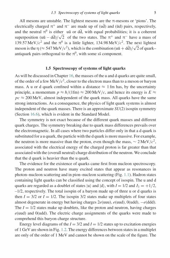
All mesons are unstable. The lightest mesons are the π-mesons or ‘pions’. Theelectrically charged π+ and π− are made up of (ud) and (ud) pairs, respectively,and the neutral π0 is either uu or dd, with equal probabilities; it is a coherentsuperposition (uu − dd)/
√2 of the two states. The π+ and π− have a mass of
139.57 MeV/c2 and the π0 is a little lighter, 134.98 MeV/c2. The next lightestmeson is the η (≈ 547 MeV/c2), which is the combination (uu + dd)/
√2 of quark–
antiquark pairs orthogonal to the π0, with some ss component.
1.5 Spectroscopy of systems of light quarks
As will be discussed in Chapter 16, the masses of the u and d quarks are quite small,of the order of a few MeV/c2, closer to the electron mass than to a meson or baryonmass. A u or d quark confined within a distance ≈ 1 fm has, by the uncertaintyprinciple, a momentum p ≈ h/(1fm) ≈ 200 MeV/c, and hence its energy is E ≈pc ≈ 200 MeV, almost independent of the quark mass. All quarks have the samestrong interactions. As a consequence, the physics of light quark systems is almostindependent of the quark masses. There is an approximate SU(2) isospin symmetry(Section 16.6), which is evident in the Standard Model.
The symmetry is not exact because of the different quark masses and differentquark charges. The symmetry breaking due to quark mass differences prevails overthe electromagnetic. In all cases where two particles differ only in that a d quark issubstituted for a u quark, the particle with the d quark is more massive. For example,the neutron is more massive than the proton, even though the mass, ∼ 2 MeV/c2,associated with the electrical energy of the charged proton is far greater than thatassociated with the (overall neutral) charge distribution of the neutron. We concludethat the d quark is heavier than the u quark.
The evidence for the existence of quarks came first from nucleon spectroscopy.The proton and neutron have many excited states that appear as resonances inphoton–nucleon scattering and in pion–nucleon scattering (Fig. 1.1). Hadron statescontaining light quarks can be classified using the concept of isospin. The u and dquarks are regarded as a doublet of states |u〉 and |d〉, with I = 1/2 and I3 = +1/2,–1/2, respectively. The total isospin of a baryon made up of three u or d quarks isthen I = 3/2 or I = 1/2. The isospin 3/2 states make up multiplets of four statesalmost degenerate in energy but having charges 2e(uuu), e(uud), 0(udd), −e(ddd).The I = 1/2 states make up doublets, like the proton and neutron, having chargese(uud) and 0(udd). The electric charge assignments of the quarks were made tocomprehend this baryon charge structure.
Energy level diagrams of the I = 3/2 and I = 1/2 states up to excitation energiesof 1 GeV are shown in Fig. 1.2. The energy differences between states in a multipletare only of the order of 1 MeV and cannot be shown on the scale of the figure. The

6 The particle physicist’s view of Nature
Figure 1.1 The photon cross-section for hadron production by photons on protons(dashes) and deuterons (crosses). The difference between these cross-sections isapproximately the cross-section for hadron production by photons on neutrons.(After Armstrong et al. (1972).)
widths of the excited states are however quite large, of the order of 100 MeV,corresponding to mean lives τ = h/ ∼ 10−23s. The excited states are all energeticenough to decay through the strong interaction, as for example ++ → p + π+
(Fig. 1.3).

N (939)
∆ (1232)
Excitation energy(GeV)
I = 12
3+
2
7+
2
1+
2
3+
2
5+
2
3+
2
3+
2
5+
2
3+
21+
2
1+
2
3−
2
5−
2 1−
2
1−
2
1−
2
5−
2
3−
2
1−
2
I = 32
1.0
0.5
0.0
Figure 1.2 An energy-level diagram for the nucleon and its excited states. Thelevels fall into two classes: isotopic doublets (I = 1/2) and isotopic quartets (I =3/2). The states are labelled by their total angular momenta and parities JP . Thenucleon doublet N(939) is the ground state of the system, the (1232) is the lowestlying quartet. Within the quark model (see text) these two states are the lowest thatcan be formed with no quark orbital angular momentum (L = 0). The other statesdesignated by unbroken lines have clear interpretations: they are all the next mostsimple states with L = 1 (negative parity) and L = 2 (positive parity). The brokenlines show states that have no clear interpretation within the simple three-quarkmodel. They are perhaps associated with excited states of the gluon fields.

8 The particle physicist’s view of Nature
Table 1.4. Isospin quantum numbersof light quarks
Quark Isospin I I3
u 1/2 1/2u 1/2 −1/2d 1/2 −1/2d 1/2 1/2s 0 0s 0 0
Figure 1.3 A quark model diagram of the decay ++ → p + π+. The gluon fieldis not represented in this diagram, but it would be responsible for holding the quarksystems together and for the creation of the dd pair.
The rich spectrum of the baryon states can largely be described and understoodon the basis of a simple ‘shell’ model of three confined quarks. The lowest stateshave orbital angular momentum L = 0 and positive parity. The states in the nextgroup have L = 1 and negative parity, and so on. However, the model has the curiousfeature that, to fit the data, the states are completely symmetric in the interchangeof any two quarks. For example, the ++(uuu), which belongs to the lowest I =3/2 multiplet, has J p = 3/2+. If L = 0 the three quark spins must be aligned ↑↑↑in a symmetric state to give J = 3/2, and the lowest energy spatial state must betotally symmetric. Symmetry under interchange is not allowed for an assembly ofidentical fermions! However, there is no doubt that the model demands symmetry,and with symmetry it works very well. The resolution of this problem will be leftto later in this chapter. There are only a few states (broken lines in Fig. 1.2) thatcannot be understood within the simple shell model.
Mesons made up of light u and d quarks and their antiquarks also have a richspectrum of states that can be classified by their isospin. Antiquarks have an I3 ofopposite sign to that of their corresponding quark (Table 1.4.). By the rules for theaddition of isospin, quark–antiquark pairs have I = 0 or I = 1. The I = 0 states

1.5 Spectroscopy of systems of light quarks 9
1−
0−
1−
0−
1+
(a)
States are predominantly ss
(b) (c)Mass(GeV)
(c)
1+
2+
0+
0+
2+
2+
1+
0+
1+
0+
1.5
1.0
0.5
0.0
1+
1+
0+
1−
1−
0−
I = 0 I = 1 I = 12
Figure 1.4 States of the quark–antiquark system uu, ud, du, dd form isotopic triplets(l = 1) : ud, (uu − dd)/
√2, du; and also isotopic singlets (I = 0) : (uu + dd)/
√2.
Figure 1.4(a) is an energy-level diagram of the lowest energy isosinglets, includingstates --- which are interpreted as ss states. Figure 1.4(b) is an energy-level diagramof the lowest energy isotriplets. Figure 1.4(c) is an energy-level diagram of thelowest energy K mesons. The K mesons are quark–antiquark systems us and ds;they are isotopic doublets, as are their antiparticle states su and sd. Their higherenergies relative to the states in Fig. 1.4(b) are largely due to the higher mass ofthe s over the u and d quarks. The large relative displacement of the 0+ state is afeature with, as yet, no clear interpretation.
are singlets with charge 0, like the η (Fig. 1.4(a)). The I = 1 states make up tripletscarrying charge +e, 0, −e, which are almost degenerate in energy, like the tripletπ+, π0, π−.
The spectrum of I = 1 states with energies up to 1.5 GeV is shown in Fig. 1.4(b).As in the baryon case the splitting between states in the same isotopic multipletis only a few MeV; the widths of the excited states are like the widths of the

10 The particle physicist’s view of Nature
excited baryon states, of the order of 100 MeV. In the lowest multiplet (the pions),the quark–antiquark pair is in an L = 0 state with spins coupled to zero. HenceJ P = 0−, since a fermion and antifermion have opposite relative parity (Section6.4). In the first excited state the spins are coupled to 1 and J P = 1−. These arethe ρ mesons. With L = 1 and spins coupled to S = 1 one can construct states2+, 1+, 0+, and with L = 1 and spins coupled to S = 0 a state 1+. All these statescan be identified in Fig. 1.4(b).
1.6 More quarks
‘Strange’ mesons and baryons were discovered in the late 1940s, soon after thediscovery of the pions. It is apparent that as well as the u and d quarks there existsa so-called strange quark s, and strange particles contain one or more s quarks. Ans quark can replace a u or d quark in any baryon or meson to make the strangebaryons and strange mesons. The electric charges show that the s quark, like thed, has charge –e/3, and the spectra can be understood if the s is assigned isospinI = 0.
The lowest mass strange mesons are the I = 1/2 doublet, K−(su, mass 494 MeV)and Ko(sd, mass 498 MeV). Their antiparticles make up another doublet, the K+(us)and Ko(ds).
The effect of quark replacement on the meson spectrum is illustrated inFig. 1.4. Each level in the spectrum of Fig. 1.4(b) has a member (du) with charge −e.Figure 1.4(c) shows the spectrum of strange (su) mesons. There is a correspondencein angular momentum and parity between states in the two spectra. The energy dif-ferences are a consequence of the s quark having a much larger mass, of the orderof 200 MeV.
The excess of mass of the s quark over the u and d quarks makes the s quark inany strange particle unstable to decay by the weak interaction.
Besides the u, d and s quarks there are considerably heavier quarks: thecharmed quark c (mass ≈ 1.3 GeV/c2, charge 2e/3), the bottom quark b (mass ≈4.3 GeV/c2, charge −e/3), and the top quark t (mass ≈ 180 GeV/c2, charge 2e/3).The quark masses are most remarkable, being even more disparate than the leptonmasses. The experimental investigation of the elusive top quark is still in its infancy,but it seems that three quarks of any of the six known flavours can be bound to forma system of states of a baryon (or three antiquarks to form antibaryon states), andany quark–antiquark pair can bind into mesonic states.
The c and b quarks were discovered in e+ e− colliding beam machines. Veryprominent narrow resonances were observed in the e+ e− annihilation cross-sections. Their widths, of less than 15 MeV, distinguished the meson states respon-sible from those made up of u, d or s quarks. There are two groups of resonant states.

1.7 Quark colour 11
The group at around 3 GeV centre of mass energy are known as J/ψ resonances,and are interpreted as charmonium cc states. Another group, around 10 GeV, the ϒ
(upsilon) resonances, are interpreted as bottomonium bb states. The current state ofknowledge of the cc and bb energy levels is displayed in Fig. 1.5. We shall discussthese systems in Chapter 17.
The existence of the top quark was established in 1995 at Fermilab, in pp colli-sions.
1.7 Quark colour
Much informative quark physics has been revealed in experiments with e+ e− col-liding beams. We mention here experiments in the range between centre of massenergies 10 GeV and the threshold energy, around 90 GeV, at which the Z bosoncan be produced.
The e+ e− annihilation cross-section σ(e+ e− → µ+ µ−) is comparatively easyto measure, and is easy to calculate in the Weinberg–Salam electroweak theory,which we shall introduce in Chapter 12. At centre of mass energies much below 90GeV the cross-section is dominated by the electromagnetic process represented bythe Feynman diagram of Fig. 1.6. The muon pair are produced ‘back-to-back’ in thecentre of mass system, which for most e+ e− colliders is the laboratory system. Toleading order in the fine-structure constant α = e2/(4πε0hc), the differential cross-section for producing muons moving at an angle θ with respect to unpolarisedincident beams is
dσ
dθ= πα2
2s(1 + cos2 θ ) sin θ (1.1)
where s is the square of the centre of mass energy (see Okun, 1982, p. 205). In thederivation of (1.1) the lepton masses are neglected. Integrating with respect to θ ,the total cross-section is
σ = 4πα2
3s. (1.2)
The quantity R(E) shown in Fig. 1.7 is the ratio
R = σ (e+ e− → strongly interacting particles)
σ (e+ e− → µ+ µ−). (1.3)
At the lower energies many hadronic states are revealed as resonances, but R seemsto become approximately constant, R ≈ 4, at energies above 10 GeV up to about40 GeV.

4.0
Mass (GeV/c2)
Mass (GeV/c2)
2S
IP
IS
cc
3.5
3.0
10.5
10.0
3S
2S
1S
bb
2P
1P
9.5
Figure 1.5 Energy-level diagrams for charmonium cc and bottomonium bb states,below the threshold at which they can decay through the strong interaction tomeson pairs (for example cc → cu + uc). States labelled 1S, 2S, 3S have orbitalangular momentum L = 0 and the 1P, 2P states have L = 1. The intrinsic quarkspins can couple to S = 0 to give states with total angular momentum J = L.These states are denoted by -----; experimentally they are difficult to detect. Theintrinsic quark spins can also couple to give S = 1. States with S = 1 are denotedby —. Spin–orbit coupling splits the P states with S = 1 to give rise to states withJ P = 0+, 1+, 2+. This spin–orbit splitting is apparent in the figure. All the S = 1states shown have been measured.

1.7 Quark colour 13
Figure 1.6 The lowest order Feynman diagram (Chapter 8) for electromagneticµ+ µ− pair production in e+e− collisions.
As fundamental particles, quarks have the same electrodynamics as muons, apartfrom the magnitude of their electric charge. The Feynman diagrams that dominatethe numerator of R in this range 10 GeV to 40 GeV are shown in Fig. 1.8. (The topquark has a mass ∼ 174 GeV/c2 and will not contribute.) For each quark processthe formula (1.2) holds, except that e is replaced by the quark’s electric charge atthe quark vertex, which suggests
R =(
2
3
)2
+(
1
3
)2
+(
2
3
)2
+(
1
3
)2
+(
1
3
)2
= 11
9. (1.4)
This value is too low, by a factor of about 3.In the Standard Model, the discrepancy is resolved by introducing the idea of
quark colour. A quark not only has a flavour index, u, d, s, c, b, t, but also, for eachflavour, a colour index. There are postulated to be three basic states of colour, sayred, green and blue (r, g, b). With three quark colour states to each flavour, we haveto multiply the R of (1.4) by 3, to obtain
R = 11
3, (1.5)
which is in excellent agreement with the data of Fig. 1.7.This invention of colour not only solves the problem of R but, most significantly,
solves the problem of the symmetry of the baryon states. We have seen (Section1.5) that in the absence of any new quantum number baryon states are completelysymmetric in the interchange of two quarks. However, if these state functions aremultiplied by an antisymmetric colour state function, the overall state becomesantisymmetric, and the Pauli principle is preserved.
Strong support for the mechanism of quark production represented by theFeynman diagrams of Fig. 1.8 is given by other features in the data frome+ e− colliders. An e+ e− annihilation at high energies produces many hadrons.

14 The particle physicist’s view of Nature
Figure 1.7 Measurements of R(E) from the resonance region 1 GeV < E < 11 GeVinto the region 11 GeV < E < 60 GeV, which contains no prominent resonancesand no quark–antiquark production threshold. For E > 11 GeV two curves areshown of calculations that take account of quark colour and include electroweakcorrections and strong interaction (QCD) effects. (Adapted from Particle DataGroup (1996).)
Figure 1.8 The lowest order Feynman diagrams for quark–antiquark pair produc-tion in e+ e− collisions at energies below the Z threshold.

1.7 Quark colour 15
Figure 1.9 An example of an e+ e− annihilation event that results in two jets ofhadrons. The figure shows the projection of the charged particle tracks onto a planeperpendicular to the axis of the e+ e− beams. This figure was taken from an eventin the TASSO detector at PETRA DESY.
These are mostly correlated into two back-to-back jets. An example is shown inFig. 1.9. (The charged particle tracks are curved because of the presence of anexternal magnetic field: the curvature is related to the particle’s momentum.) Thedirection of a jet may be defined as the direction at the point of production of thetotal momentum of all the hadrons associated with it. The momenta of two back-to-back jets are equal and opposite. The jet directions may be presumed to be thedirections of the initial quark–antiquark pair. This interpretation is corroborated byan examination of the angular distribution of the jet directions of two-jet eventsfrom many annihilations, with respect to the e+ e− beams. The angular distributionis the same as that for muons (equation (1.1)) after allowance has been made forthe Z contribution, which becomes significant as the energy for Z production isapproached.

16 The particle physicist’s view of Nature
The hadron jets result from the original quark and antiquark combining withquark–antiquark pairs generated from the vacuum. The precise details of the pro-cesses involved are not yet fully understood.
1.8 Electron scattering from nucleons
There is a clear advantage in using electrons to probe the proton and neutron, sinceelectrons interact with quarks primarily through electromagnetic forces that arewell understood: the weak interaction is negligible in the scattering process, exceptat very high energy and large scattering angle, and the strong interaction is notdirectly involved.
In the 1950s, experiments at Stanford on nucleon targets at rest in the laboratoryrevealed the electric charge distribution in the proton and (using scattering datafrom deuterium targets) the neutron. These early experiments were performed atelectron energies ≤ 500 MeV (Hofstadter et al., 1958). Scattering at higher ener-gies has thrown more light on the behaviour of quarks in the proton. At theseenergies inelastic electron scattering, which involves meson production, becomesthe dominant mode.
At the electron–proton collider HERA at Hamburg, a beam of 30 GeV electronsmet a beam of 820 GeV protons head on. Many features of the ensuing electron–proton collisions are well described by the parton model, which was introducedby Feynman in 1969. In the parton model each proton in the beam is regarded asa system of sub-particles called partons. These are quarks, antiquarks and gluons.Quarks and antiquarks are the particles that carry electric charge. The basic idea ofthe parton model is that at high energy–momentum transfer Q2, an electron scattersfrom an effectively free quark or antiquark and the scattering process is completedbefore the recoiling quark or antiquark has time to interact with its environment ofquarks, antiquarks and gluons. Thus in the calculation of the inclusive cross-sectionthe final hadronic states do not appear.
In the model, at large Q2 both the electron and the struck quark are deflectedthrough large angles. Figure 1.10 shows an example of an event from the ZEUSdetector at HERA. The transverse momentum of the scattered electron is balancedby a jet of hadrons, which can be associated with the recoiling quark. Another jet,the ‘proton remnant’ jet is confined to small angles with respect to the proton beam.Events like these give further strong support to the parton model.
The success of the parton model in interpreting the data gives added support tothe concept of quarks. The parton model is not strictly part of our main theme but,in view of its interest and importance in particle physics, a simple account of themodel and its relation to experiment is given in Appendix D.

1.9 Particle accelerators 17
(a)
e
e
(b)
30 GeVelectron beam
820 GeVproton beam
Figure 1.10 This figure illustrating particle tracks is taken from an event in theZEUS detector at HERA, DESY. Figure 1.10(a) is the event projected onto a planeperpendicular to the axis of the beams. Figure 1.10(b) is the event projected ontoa plane passing through the axis of the beams.
A hadron jet has been ejected from the proton by an electron. The track of therecoiling electron is marked e. The initiating beams and the proton remnant jet areconfined to the beam pipes and are not detected.
1.9 Particle accelerators
Progress in our understanding of Nature has come through the interplay betweentheory and experiment. In particle physics, experiment now depends primarily onthe great particle accelerators and ingeneous and complex particle detectors, whichhave been built, beginning in the early 1930s with the Cockroft–Walton linearaccelerator at Cambridge, UK, and Lawrence’s cyclotron at Berkeley, USA. TheCambridge machine accelerated protons to 0.7 MeV; the first Berkeley cyclotronaccelerated protons to 1.2 MeV. For a time after 1945 important results wereobtained using cosmic radiation as a source of high energy particles, eventsbeing detected in photographic emulsion, but in the 1950s new accelerators

18 The particle physicist’s view of Nature
Table 1.5. Some particle accelerators
Machine Particles collided Start date–end date
TEVATRON p: 900 GeV 1987(Fermilab, Batavia, Il) p : 900 GeV
SLC e+ : 50 GeV 1989–1998(SLAC, Stanford) e− : 50 GeV
HERA e: 30 GeV 1992(DESY, Hamburg) p: 820 GeV
LEP2 e+ : 81GeV 1996–2000(CERN, Geneva) e− : 81GeVPEP-II e− : 9 GeV 1999–2008(SLAC, Stanford) e+ : 3.1 GeVLHC p: 7 TeV 2008(CERN, Geneva) p: 7 TeV
provided beams of particles of increasingly high energies. Some of the machines,past, present and future, are listed in Table 1.5.. Detailed parameters of thesemachines, and of others, may be found in Particle Data Group (2005).
The TEVATRON at Fermilab is where the top quark was discovered. The physicsof the top quark is as yet little explored. It makes only a brief appearance in our text,though it is an essential part of the pattern of the Standard Model. The upgradedLEP2 at CERN is able to create W+ W− pairs, and will allow detailed studies ofthe weak interaction. At Stanford, PEP-II and the associated ‘BaBar’ (BB) detectoris designed to study charge conjugation, parity (CP) violation. The way in whichCP violation appears in the Standard Model is discussed in Chapter 18.
The most ambitious machine likely to be built in the immediate future is theLarge Hadron Collider (LHC) at CERN. It is expected that with this machine it willbe possible to observe the Higgs boson, if such a particle exists. The Higgs boson isan essential component of the Standard Model; we introduce it in Chapter 10. It isalso widely believed that the physics of Supersymmetry, which perhaps underliesthe Standard Model, will become apparent at the energies, up to 14 TeV, which willbe available at the LHC.
1.10 Units
In particle physics it is usual to simplify the appearance of equations by using unitsin which h = 1 and c = 1. In electromagnetism we set ε0 = 1 (so that the forcebetween charges q1 and q2 is q1q2/4πr2), and µ0 = 1, to give c2 = (µ0ε0)−1 = 1.

1.10 Units 19
We shall occasionally reinsert factors of h and c where it may be reassuringor illuminating, or for the purposes of calculation. It is useful to rememberthat
hc ≈ 197 MeV fm, e2 4π ≈ 1.44 MeV fm,
α = e2/4πhc ≈ (1/137), c ≈ 3 × 10²³ fm s−1.
Energies, masses and momenta are usually quoted in MeV or GeV, and we shallfollow this convention.

2
Lorentz transformations
The equations of the Standard Model must be consistent with Einstein’s principleof relativity, which states that the laws of Nature take the same form in everyinertial frame of reference. An inertial frame is one in which a free body moveswithout acceleration. An earth-bound frame approximates to an inertial frame if thegravitational field of the earth is introduced as an external field. We shall assumethat the reader is familiar with rotations, and with proper Lorentz transformationsand the relativistic mechanics of particle collisions. This chapter is very largelyabout notation, which may make for dry reading; however an appropriate notationis crucial to the exposition of any theory, and particularly so to a relativistic theory,such as the Standard Model.
2.1 Rotations, boosts and proper Lorentz transformations
The time and space coordinates of an event measured in different inertial framesof reference are related by a Lorentz transformation. A rotation is a special case ofa Lorentz transformation. Consider, for example, a frame K ′ that is rotated aboutthe z-axis with respect to a frame K, by an angle θ . If (t, r) are the time and spacecoordinates of an event observed in K, then in K ′ the event is observed at (t′, r′)and
t ′ = tx ′ = x cos θ + y sin θ
y′ = −x sin θ + y cos θ
z′ = z.
(2.1)
Lorentz transformations also relate events observed in frames of reference thatare moving with constant velocity, one with respect to the other. Consider, forexample, an inertial frame K ′ moving in the z-direction in a frame K with velocityv, the spatial axes of K and K ′ being coincident at t = 0. If (t, r) are the time and
20

2.1 Rotations, boosts and proper Lorentz transformations 21
space coordinates of an event observed in K, and (t′, r′) are the coordinates of thesame event observed in K ′, the transformation takes the form
ct ′ = γ (ct − βz)x ′ = xy′ = yz′ = γ (z − βct),
(2.2)
where c is the velocity of light, β = υ/c, γ = (1 − β2)−1/2.Putting x0 = ct, x1 = x, x2 = y, x3 = z, the xµ are dimensionally homoge-
neous, and an event in K is specified by the set xµ, where µ = 0, 1, 2, 3. Greekindices in the text will in general take these values. With this more convenientnotation, we may write the Lorentz transformation (2.2) as
x ′0 = x0 cosh θ − x3 sinh θ
x ′1 = x1
(2.3)x ′2 = x2
x ′3 = −x0 sinh θ + x3 cosh θ,
where we have put β = v/c = tanh θ ; then γ = cosh θ .Transformations to a frame with parallel axes but moving in an arbitrary direc-
tion are called boosts. A general Lorentz transformation between inertial frames Kand K ′ whose origins coincide at x0 = x ′0 = 0 is a combination of a rotation anda boost. It is specified by six parameters: three parameters to give the orientationof the K ′ axes relative to the K axes, and three parameters to give the compo-nents of the velocity of K ′ relative to K. Such a general transformation is of theform
x ′µ = Lµνxν, (2.4)
where the elements Lµν of the transformation matrix are real and dimensionless.
We use here, and subsequently, the Einstein summation convention: a repeated‘dummy’ index is understood to be summed over, so that in (2.4) the notation∑3
ν=0 has been omitted on the right-hand side. The matrices Lµν form a group,
called the proper Lorentz group (Problem 2.6 and Appendix B). The significanceof the placing of the superscript and the subscript will become evident shortly.
The interval (s)2 between events xµ and xµ + xµ is defined to be
(s)2 = (x0)2 − (x1)2 − (x2)2 − (x3)2. (2.5)
It is a fundamental property of a Lorentz transformation that it leaves the intervalbetween two events invariant:
(s ′)2 = (s)2. (2.6)

22 Lorentz transformations
We can express (s)2 more compactly by introducing the metric tensor (gµν):
(gµν) =
1 0 0 00 −1 0 00 0 −1 00 0 0 −1
. (2.7)
Then
(s)2 = gµνxµxν, (2.8)
where the repeated upper and lower indices are summed over. Note that gµν = gνµ;it is a symmetric tensor. It has the same elements in every frame of reference.
2.2 Scalars, contravariant and covariant four-vectors
Quantities, such as (s)2, which are invariant under Lorentz transformations arecalled scalars. We define a contravariant four-vector to be a set aµ which transformslike the set xµ under a proper Lorentz transformation:
a′µ = Lµνaν. (2.9)
A familiar example of a contravariant four-vector is the energy–momentum vectorof a particle (E/c, p).
We define the corresponding covariant four-vector aµ, carrying a subscript,rather than a superscript, by
aµ = gµνaν. (2.10)
Hence if aµ = (a0, a), then aµ = (a0, −a).We can write the invariant s2 as
s2 = gµνxµxν = xνxν.
More generally, if aµ, bµ are contravariant four-vectors, the scalar product
gµνaµbν = aµbµ = aµbµ = a0b0 − a·b (2.11)
is invariant under a Lorentz transformation.We can define the contravariant metric tensor gµν so that
αµ = gµνaν. (2.12)
The elements of gµν are evidently identical to those of gµν .The transformation law for covariant vectors, which we write
a′µ = Lµ
νaν, (2.13)

2.3 Fields 23
follows from that for contravariant vectors (Problem 2.1). Note that, in general,Lµ
ν is not equal to Lνµ (Problem 2.1). Using the invariance of the scalar product
(2.11), we have
a′µb′µ = Lµ
ν Lµρaνbp = aνbν
and
a′µb′µ = Lµ
ν Lµρaν bρ = aν bν .
Since the aµ and bµ are arbitrary, it follows that
Lµν Lµ
ρ = Lµν Lµ
ρ = δρν (2.14)
where
δρν = δν
ρ =
1, ρ = ν
0, ρ = ν.
2.3 Fields
The Standard Model is a theory of fields. We shall be concerned with fields that ateach point x of space and time transform as scalars, or vectors, or tensors (definedlater in this section). We use x to stand for the set (x0, x1, x2, x3). For example,we shall see that the electromagnetic potentials form a four-vector field, and theelectromagnetic field is a tensor field. We shall also be concerned with scalar fieldsφ(x), which by definition transform simply as
φ′(x ′) = φ(x), (2.15)
where x′ and x refer to the same point in space-time.We can construct a vector field from a scalar field. Consider the change of field
dφ in moving from x to a neighbouring point x + dx, with dx infinitesimal. Then
dφ = ∂φ
∂xµdxµ
is invariant under a Lorentz transformation. Since the set dxµ make up an arbitrarycontravariant infinitesimal vector, the set ∂φ/∂xµ must make up a covariant vector(Problem 2.3). Following the subscript convention we write
∂φ
∂xµ=
(1
c
∂φ
∂t, ∇φ
)= ∂µφ. (2.16)
We can then also define the contravariant vector
∂µφ = gµν∂νφ = ∂φ
∂xµ
=(
1
c
∂φ
∂t, −∇φ
). (2.17)

24 Lorentz transformations
It follows that
∂µφ∂µφ =(
1
c
∂φ
∂t
)2
− (∇φ)2 (2.18)
and
∂µ∂µφ = 1
c2
∂2φ
∂t2− ∇2φ (2.19)
are invariant under Lorentz transformations.We can define, and we shall need, tensor quantities. Tensors T µν, Tµν, T µ
ν, T µνλ,
etc., are defined as quantities which transform under a Lorentz transformation inthe same way as aµaν, aµaν, aµaν, aµaνaλ, etc. For example,
T ′µν = Lµρ Lν
λT ρλ.
The ‘contraction’ by summation of a repeated upper and lower index leavesthe transformation properties determined by what remains. For example, T µ
µ is ascalar, T µν
µ is a contravariant four-vector. The metric tensors gµν, gµν conformwith the definition, and this leads to the conditions on the matrix elements Lµ
ν :
gµν = gpλLρµLλ
ν. (2.20)
The conditions (2.20) and (2.14) are equivalent.As well as scalars, vectors and tensors there are also very important objects
called spinors, and spinors fields, which have well-defined rules of transformationunder a Lorentz transformation of the coordinates. Their properties are discussedin Appendix B and Chapter 5.
2.4 The Levi–Civita tensor
The Levi–Civita tensor εµνλρ is defined by
εµνλρ =
+1 if µ, ν, λ, ρ is an even permutation of 0, 1, 2, 3;−1 if µ, ν, λ, ρ is an odd permutation of 0, 1, 2, 3;
0 otherwise.(2.21)
For example, ε1023 = −1, ε1203 = +1, ε0023 = 0.It is straightforward to verify that εµνλρ satisfies
ε′µνλρ = Lµ
α Lνβ Lλ
γ Lρδεαβγ δ
= εµνλµ det(L) = εµνλµ,
using the definition of a determinant (Appendix A), and the result that the determi-nant of the transformation matrix is 1 (Problems 2.4 and 2.5).

Problems 25
The corresponding Levi–Civita symbol in three dimensions, εi jk , is defined sim-ilarly. It is useful in the construction of volumes, since
εi jk Ai B j Ck = A · (B × C)
is the volume of the parallelepiped defined by the vectors A, B, C. The four-dimensional Levi–Civita tensor enables one to construct four-dimensional volumesεµνλρaµbνcλdρ . The contraction of indices leaves this a Lorentz scalar. In partic-ular, taking a,b,c,d to be infinitesimal elements parallel to the axes 0xµ so thata = (dx0, 0, 0, 0), b = (0, dx1, 0, 0), c = (0, 0, dx2, 0), d = (0, 0, 0, dx3), it fol-lows that the ‘volume’ element of space-time
d4x = dx0dx1dx2dx3 = cd3x dt
is a Lorentz invariant scalar (see also Problem 2.9).
2.5 Time reversal and space inversion
The operations of time reversal:
x ′0 = −x0,
x ′ i = xi , i = 1, 2, 3,
and space inversion:
x ′0 = x0
x ′ i = −xi , i = 1, 2, 3,
also leave (s)2 invariant, but these transformations are excluded from the properLorentz group. They are however of interest, and will arise in later chapters.
Problems
2.1 Show that Lµν = gµρ Lρ
λgλν . Verify L01 = −L1
0.
2.2 Using (2.14), show that the inverse transformations to (2.9) and (2.13) are
aµ = a′ν Lνµ, aµ = a′
ν Lνµ.
Hence show
LνµLρ
µ = δρν .
2.3 Prove that if φ(x) is a scalar field, the set (∂φ/∂xµ) makes up a covariant vectorfield.

26 Lorentz transformations
2.4 Using Problem 2.1, show that det(Lµν) = det(Lµ
ν) and hence show, using equation(2.14), that
det(Lµν) = ±1.
2.5 Show that det(Lµν) for both the rotation (2.1) and the boost (2.3) is equal to +1.
This is a general property of proper Lorentz transformations that distinguishes themfrom space reflections and time reversal (Section 2.5), for which the determinant ofthe transformation equals −1.
2.6 Show that the matrices Lµν corresponding to proper Lorentz transformations form
a group.
2.7 Show that δµν is a tensor.
2.8 The frequency ω and wave vector k of an electromagnetic wave in free space makeup a contravariant four-vector
k = (ω/c, k).
The invariant kµkµ = 0; this corresponds to the dispersion relation ω2 = c2k2. Showthat a wave propagating with frequency ω in the z-direction, if viewed from a framemoving along the z-axis with velocity v, is seen to be Doppler shifted in frequency,with
ω′ = e−θω =√
1 − v/c
1 + v/cω.
2.9 By considering the Jacobian of the Lorentz transformation, show that the four-dimensional volume element d4x = dx0dx1dx2dx3 is a Lorentz invariant.
2.10 Show that εµνλρ is a pseudo-tensor, i.e. it changes sign under the operation of spaceinversion.

3
The Lagrangian formulation of mechanics
In most introductory texts on quantum mechanics you will find ‘Hamiltonian’ in theindex (see our equation (3.8)) but you are less likely to find ‘Lagrangian’. However,quantum field theories are most conveniently described in a Lagrangian formalism,to which this chapter is an introduction.
3.1 Hamilton’s principle
The classical dynamics of a mechanical (non-dissipative) system is most elegantlyderived from Hamilton’s principle. A closed mechanical system is completely char-acterised by its Lagrangian L(q, q); the variables q(t), which are functions of time,are a set of coordinates q1(t),q2(t), ..., qs(t) which determine the configuration ofthe system at time t. In particular, the qi might be the Cartesian coordinates of a setof interacting particles. We restrict our discussion to the case where all the qi (t) areindependent. In non-relativistic mechanics we take L = T − V , where T (q, q) isthe kinetic energy of the system and V(q) is its potential energy.
Given L, the action S is defined by
S =∫ t2
t1
L(q, q) dt. (3.1)
The value of S depends on the path of integration in q-space. The end-points ofthe path are fixed at times t1 and t2, but the path is otherwise unrestricted. S issaid to be a functional of q(t). Hamilton’s principle states that S is stationary forthat particular path in q-space determined by the equations of motion, so that if weconsider a variation to an arbitrary neighbouring path (Fig. 3.1), δS = 0, where
δS = δ
∫ t2
t1
L(q, q) dt
=∫ t2
t1
∑i
[∂L
∂qiδqi + ∂L
∂ qδqi
]dt .
27

28 The Lagrangian formulation of mechanics
Figure 3.1 A schematic representation of the path in q-space determined by theequations of motion (full line) and a neighbouring path (dashed line).
Since δq = d(δq)/dt , we can integrate the second term in this integral by parts, togive
δS =∫ t2
t1
∑i
[∂L
∂qi− d
dt
(∂L
∂ qi
)]δqi dt . (3.2)
The ‘end-point’ contributions from the integration by parts are zero, since δq(t1) =δq(t2) = 0.
The variations δqi (t) are arbitrary. It follows from (3.2) that the condition δS = 0requires
d
dt
(∂L
∂qi
)− ∂L
∂qi= 0, i = 1, ..., s. (3.3)
These are the Euler–Lagrange equations of motion. In classical non-relativisticmechanics they are equivalent to Newton’s equations of motion. As a simple exam-ple, consider a particle of mass m moving in one dimension in a potential V(x). ThenL = T − V = (mx2/2) − V (x). From (3.3) we have immediately mx = −∂V/∂x ,which is Newton’s equation of motion for the particle.
An external, and possibly time-dependent, field can be included in the Lagrangianformalism through a time-dependent potential. In our one-dimensional exampleabove, V(x) may be replaced by V(x,t). Making the Lagrangian L depend explicitlyon t does not affect the derivation of the field equations.

3.2 Conservation of energy 29
It is important to note that the Lagrangian of a given system is not unique: wecan add to L any function of the form df (q,t)/dt where f(q,t) is an arbitrary functionof q and t. Such a term gives a contribution [ f (q2, t2) − f (q1, t1)] to S, independentof the path, and hence leaves the equations of motion unchanged.
3.2 Conservation of energy
In the case of a closed system of particles, interacting only among themselves, theequations of motion of the system do not depend explicitly on the time t, since thephysics of a closed system does not depend on our choice of the origin of time.There is no reason to doubt that the laws of physics at the time of Archimedes, orthe time of Newton, were the same as they are for us. Hence for a closed systemwe must be able to construct a Lagrangian L(q, q) that does not depend explicitlyon t. For such a Lagrangian,
dL
dt=
∑i
[∂L
∂qiqi + ∂L
∂ qiqi
].
Taking the qi(t) to obey the equations of motion and substituting for ∂L/dqi from(3.3) we obtain
dL
dt=
∑i
[(d
dt
∂L
∂qi
)qi + ∂L
∂qiqi
]=
∑i
d
dt
(∂L
∂qiqi
)or
d
dt
[∑i
∂L
∂qiqi − L
]= 0. (3.4)
Thus
E =[∑
i
∂L
∂qiqi − L
](3.5)
remains constant during the motion, and is called the energy of the system. Thisresult exemplifies Noether’s theorem (Section 1.2): we have here a conservationlaw stemming from the symmetry of the Lagrangian under a translation in time.
For a closed system of non-relativistic particles, with a potential functionV (qi ), ∂L/∂qi = ∂T/∂qi . Since the kinetic energy T is a quadratic function ofthe qi (Problem 3.1), (∂T/∂qi )qi = 2T . Hence
E = 2T − (T − V ) = T + V .
We recover the result of elementary mechanics.

30 The Lagrangian formulation of mechanics
The generalised momenta, pi , are defined by
pi = ∂L
∂ qi. (3.6)
The Hamiltonian of a system is defined by
H (p, q) =∑
i
pi qi − L. (3.7)
In terms of p and q, the energy equation (3.5) for a closed system becomes
H (p, q) = E . (3.8)
This equation, which is a consequence of the homogeneity of time, is a foundationstone for making the transition from classical to quantum mechanics.
3.3 Continuous systems
To see how Hamilton’s principle may be extended to continuous systems, we con-sider a flexible string, of mass ρ per unit length, stretched under tension F betweentwo fixed points at x = 0 and x = l, say, but subject to small transverse displace-ments in a plane. Gravity is neglected. If φ(x, t) is the transverse displacement fromequilibrium of an element dx of the string at x, at time t, then the length of the stringis ∫ l
0(dx2 + dφ2)1/2 =
∫ l
0[1 + (∂φ/∂x)2]1/2dx .
To leading order in ∂φ/∂x , which we take to be small for small displacements,the extension of the string is
∫ l0
12 (∂φ/∂x)2dx , and the potential energy of stretch-
ing under the tension F is∫ 1
012 F(∂φ/∂x)2dx . The kinetic energy of the string is∫ 1
012ρ(∂φ/∂t)2dx . Hence
L = T − V =∫ 1
0L dx, (3.9)
where
L = 1
2ρ
(∂φ
∂t
)2
− 1
2F
(∂φ
∂x
)2
(3.10)
is called the Lagrangian density.The corresponding action is
S =∫ 1
0dx
∫ t2
t1
dtL(φ, φ′),
writing ∂φ/∂t = φ and ∂φ/∂x = φ′.

3.3 Continuous systems 31
Figure 3.2 The actual motion of the string between an initial displacement φ(x, t1)and a final displacement φ(x, t2) generates a surface in space-time.
Hamilton’s principle states that the action is stationary for that surface thatdescribes the actual motion of the string between its initial displacement φ(x, t1)and its final displacement φ(x, t2) (Fig. 3.2). We have
δS =∫ 1
0dx
∫ t2
t1
dt
[∂L
∂φδ(φ) + ∂L
∂φ′ δ(φ′)].
Using δ(φ) = ∂(δφ)/∂t and δ(φ′) = ∂(δφ)/dx we integrate each term by parts.Again, the boundary contributions are zero since
δφ(x, t1) = δφ(x, t2) = 0 for all x,
δφ(0, t) = δφ(l, t) = 0 for all t.
We are left with
δS = −∫ 1
0dx
∫ t2
t1
dt
[∂
∂t
(∂L
∂φ
)+ ∂
∂x
(∂L
∂φ′
)]δφ. (3.11)
Since δφ(x, t) is arbitrary, the condition δS = 0 gives
∂
∂t
(∂L
∂φ
)+ ∂
∂x
(∂L
∂φ′
)= 0. (3.12)

32 The Lagrangian formulation of mechanics
Inserting the Lagrangian density (3.10), we obtain the familiar wave equationfor small amplitude waves on a string:
ρ∂2φ
∂t2− F
∂2φ
∂x2= 0.
Thus continuous systems can be described in a Lagrangian formalism by a suitablechoice of Lagrangian density, and clearly the method can be extended to wavesin any number of dimensions. By analogy with (3.6) and (3.7), we can define themomentum density
(φ) = ∂L
∂φ
and the Hamiltonian density
H = φ − L. (3.13)
Since the Lagrangian density (3.10) does not depend explicitly on t, it follows that
E =∫
H dx =∫ (
∂L
∂φφ − L
)dx (3.14)
remains constant during the motion (Problem 3.2). This result is the analogue of(3.5).
3.4 A Lorentz covariant field theory
In three spatial dimensions, the action is of the form
S =∫
L dx dy dz dt =∫
L dx0dx1dx2dx3. (3.15)
The ‘volume element’ dx0dx1dx2dx3 = d4x is a Lorentz invariant (Section 2.4).Hence S is a Lorentz invariant if the Lagrangian density L transforms like a scalarfield. The covariance of the field equations is then assured. Other symmetriesrequired of a theory may be built into L.
Consider a Lorentz invariant Lagrangian density of the form
L = L(φ, ∂µφ), (3.16)
where φ(x) = φ(x0, x) is a scalar field. At any point x in space-time, such aLagrangian density depends only on the field and its first derivatives at that point.The field theory is said to be local: there is no ‘action at a distance’. This will be animportant feature of the Standard Model. The field equation is easily derived fromthe condition δS = 0, together with the condition that the field vanishes at large

3.5 The Klein–Gordon equation 33
distances, and we find
∂L
∂φ− ∂µ
(∂L
∂(∂µφ)
)= 0. (3.17)
3.5 The Klein–Gordon equation
The Lorentz invariant Lagrangian density
L = 1
2[gµν∂µφ∂νφ − m2φ2] = 1
2[∂µφ∂µφ − m2φ2], (3.18)
where φ(x) is a real scalar field, is a particular case of (3.16). The field equation(3.17) becomes
−∂µ∂µφ − m2φ = 0,
or (− ∂2
∂t2+ ∇2 − m2
)φ = 0. (3.19)
This equation is known as the Klein–Gordon equation.The equation has wave-like solutions
φ(r, t) = a cos(k · r − ωkt + θk)
where the frequency ωk is related to the wave vector k by the dispersion relation
ω2k = k2 + m2, (3.20)
and θk is an arbitrary phase angle.For mathematical simplicity we shall take the solutions φ(r, t) to lie in a large
cube of side l, volume V = l3, and apply periodic boundary conditions, so thatk = (2πn1/ l, 2πn2/ l, 2πn3/ l) where n1, n2, n3 are any integers 0, ±1, ±2, . . .
The general solution of (3.19) is a superposition of such plane waves:
φ(r, t) = 1√V
∑k
(ak√2ωk
ei(k·r−ωt) + a∗k√
2ωke−i(k·r−ωt)
). (3.21)
The factors√
2ωk are introduced for later convenience, and the phase factors havebeen absorbed into the complex wave amplitudes ak. The sum is over all allowedvalues of k.
With the de Broglie identifications of E = ωk, p = k (recall h = 1, c = 1) thedispersion relation for ωk is equivalent to the Einstein equation for a free particle,
E2 = p2 + m2.

34 The Lagrangian formulation of mechanics
We may conjecture that the Klein–Gordon equation for φ describes a scalarparticle of mass m. There is no vector associated with a one-component scalar field,and the intrinsic angular momentum associated with such a particle is zero.
We shall see a Lagrangian density of the form (3.18) arising in the Standard Modelto describe the Higgs particle. At a less fundamental level, the overall motion ofthe π0 meson, which is an uncharged composite particle, is described by a similarLagrangian density.
3.6 The energy–momentum tensor
The equations expressing both conservation of energy and conservation of linearmomentum are obtained by considering the change in L corresponding to a uniforminfinitesimal space-time displacement
xµ → xµ + δaµ, (3.22)
where δaµ does not depend on x. The corresponding change in φ is
δφ = (∂νφ)δaν. (3.23)
Since L does not depend explicitly on the xµ,
δL = ∂L
∂φδφ + ∂L
∂(∂µφ)δ(∂µφ).
Using the field equation (3.17) for ∂L/∂φ, and the fact that δ(∂µφ) = ∂µ(δφ), wecan rewrite this as
δL = ∂µ
[(∂L
∂(∂µφ)
)δφ
],
and then, from (3.23),
δL = ∂µ
[∂L
∂(∂µφ)∂νφ
]δaν.
We have also
δL = ∂L
∂xµδaµ = δµ
ν
∂L
∂xµδaν,
where, as in (2.14),
δµν =
1, µ = ν
0, µ = ν.

3.6 The energy–momentum tensor 35
Since the δaν are arbitrary, it follows on comparing these expressions for δL that
∂µ
[∂L
∂(∂µφ)∂νφ − δµ
ν L
]= 0, (3.24)
or
∂µT µν = 0, where T µ
ν =[
∂L
∂(∂µφ)∂νφ − δµ
ν L
]. (3.25)
T µν is the energy–momentum tensor. The component
T 00 = ∂L
∂φφ − L
corresponds to the Hamiltonian density defined in equation (3.13), and is inter-preted as the energy density of the field; in a relativistic theory, the energy densitytransforms like a component of a tensor. The ν = 0 component of (3.25) may bewritten
∂
∂t(T 0
0 ) + ∇ · T0 = 0, (3.26)
and expresses local conservation of energy, with T0 = (T 10 , T 2
0 , T 30 ) interpreted as
the energy flux. Integrating (3.26) over all space and using the divergence theoremyields
∂
∂t
∫T 0
0 d3x = 0, (3.27)
provided the field vanishes at large distances. This equation expresses the overallconservation of energy.
Similarly the ν = 1, 2, 3 components of (3.24) correspond to local conservationof momentum, with the overall total momentum of the field given by
Pi =∫
T 0i d3x. (3.28)
As with the energy, the total momentum of the field is conserved if the field vanishesat large distances.
In the case of the Klein–Gordon Lagrangian density (3.19),
∂L
∂φ= φ,
and the energy density of the field is
T 00 = 1
2[φ2 + (∇φ)2 + m2φ2]. (3.29)

36 The Lagrangian formulation of mechanics
Expressing φ in terms of the field amplitudes ak and a∗k, and integrating over all
space, gives the total field energy
H =∫
T 00 d3x =
∑k
a∗kakωk. (3.30)
In obtaining this expression we have used the orthogonality of the plane waves
1
V
∫ei(k−k′)·rd3x = δkk′ .
Similarly from (3.28) the total momentum of the field can be shown to be
P =∑
k
a∗kakk. (3.31)
3.7 Complex scalar fields
It is instructive to consider also complex scalar fields = (φ1 + iφ2) /√
2 satisfyingthe Klein–Gordon equation. We shall see in Section 7.6 that if the field carriescharge q, then the field ∗ carries charge −q. The Klein–Gordon equation for acomplex field is obtained from the (real) Lagrangian density
L = ∂µ∗∂µ − m2∗. (3.32)
We introduce here a device that we shall often find useful. Instead of varying thereal and imaginary parts of to obtain the field equations, we may vary andits complex conjugate ∗ independently. These procedures are equivalent. Varying∗ in the action constructed from (3.32) yields, easily,
− ∂µ∂µ − m2 = 0. (3.33)
(Varying gives the complex conjugate of this equation.)Note that the Lagrangian density (3.32) is the sum of contributions from the
scalar fields φ1 and φ2:
L = ∂µ∗∂µ − m2∗ = 1
2
[∂µφ1∂
µφ1 − m2φ21
](3.34)
+ 1
2
[∂µφ2∂
µφ2 − m2φ22
].
The general solution of (3.33) is a superposition of plane waves of the form
= 1√V
∑k
(ak√2ωk
ei(k·r−ωt) + b∗k√
2ωke−i(k·r−ωt)
)(3.35)
where ak and bk are now independent complex numbers. The field energy becomes
H =∑
k
(a∗
kak + b∗kbk
)ωk. (3.36)

Problems 37
We shall see that we can interpret this expression as being made up of the distinctcontributions of positively and negatively charged fields. (The π+ and π− mesonsare composite particles whose overall motion is described by complex scalar fields.)
Problems
3.1 Show that the kinetic energy of a system of particles, whose positions are determinedby q(t), is a quadratic function of the qi .
3.2 Show that dE/dt = 0, where E is given by equation (3.14).
3.3 For the stretched string of Section 3.3, show that the Hamiltonian density is
H = 1
2ρ
(∂φ
∂t
)2
+ 1
2F
(∂φ
∂x
)2
.
The nth normal mode of oscillation, with wave amplitude An , is given by
φn(x, t) = An sin(knx) sin(ωnt)
where kn = nπ/ l, ωn = (F/ρ)1/2kn . Show that the total energy is An2ωn
2ρl/4 andoscillates harmonically between potential energy and kinetic energy.
3.4 Verify the expressions (3.30) and (3.31) for the energy and momentum of the scalarfield given by equation (3.21).
3.5 Show that the Schrodinger equation for the wave function ψ(r, t) of a particle of massm moving in a potential V (r) may be obtained from the Lagrangian density
L = −(1/2i)
(ψ∗ ∂ψ
∂t− ∂ψ∗
∂tψ
)− (1/2m)∇ψ∗ · ∇ψ − ψ∗V ψ.
(Note that L is real, but not Lorentz invariant.)

4
Classical electromagnetism
Maxwell’s theory of electromagnetism is, along with Einstein’s theory of grav-itation, one of the most beautiful of classical field theories. In this chapter weexhibit the Lorentz covariance of Maxwell’s equations and show how they may beobtained from Hamilton’s principle. The important idea of a gauge transformationis introduced, and related to the conservation of electric charge. We analyse someproperties of solutions of the field equations. Finally, we generalise the Lagrangianto describe massive vector fields, which will figure in later chapters.
4.1 Maxwell’s equations
In common with much of the literature, we shall use units in which the force betweencharges q1 and q2 is q1q2/4πr2, and the velocity of light c = 1. (Thus in these unitsµ0 = 1, ε0 = 1.) Maxwell’s equations then take the form
∇ · E = ρ (a), ∇ × B − ∂E
∂t= J (b),
∇ · B = 0 (c), ∇ × E + ∂B
∂t= 0 (d).
(4.1)
E and B are the electric and magnetic fields, ρ and J are the electric charge andcurrent densities. In this chapter we do not consider the dynamics of ρ and J, buttake them to be ‘external’ fields that we are free to manipulate. The inhomogeneousequations (a) and (b) are consistent with the observed fact of charge conservation,which is expressed by the continuity equation:
∂ρ
∂t+ ∇ · J = 0.
This equation takes the Lorentz invariant form
∂µ Jµ = 0 (4.2)
38

4.2 A Lagrangian density for electromagnetism 39
if we postulate that the charge-current densities
Jµ = (ρ, J) (4.3)
make up a contravariant four-vector field.Introducing a scalar potential φ and a vector potential A, the homogeneous
equations (c) and (d) of the set (4.1) are satisfied identically by
B = ∇ × A, E = −∇φ − ∂A∂t
. (4.4)
We postulate that the potentials
Aµ = (φ, A) (4.5)
make up a contravariant four-vector field also.Maxwell’s equations may be written in terms of the antisymmetric tensor Fµν ,
defined by
Fµν = ∂µ Aν − ∂ν Aµ =
0 −Ex −Ey −Ez
Ex 0 −Bz By
Ey Bz 0 −Bx
Ez −By Bx 0
. (4.6)
It is apparent that the electromagnetic field is a tensor field. For example,
F01 = ∂ A1/∂x0 − ∂ A0/∂x1 = ∂ Ax/∂t + ∂φ/∂x = −Ex .
Thus the components of the electromagnetic field transform under a Lorentz trans-formation like the elements of a tensor.
The homogeneous Maxwell equations correspond to the identitities
∂λFµν + ∂ν Fλµ + ∂µFνλ ≡ 0, (4.7)
where λ, µ, ν are any three of 0, 1, 2, 3, as the reader may easily verify. Theinhomogeneous equations take the manifestly covariant form
∂µFµν = J ν. (4.8)
For example, with ν = 0, looking at the first column of Fµν , and noting ∂µ =(∂
/∂t, ∇), gives
∇ · E = ρ.
4.2 A Lagrangian density for electromagnetism
We now seek a Lagrangian density L that will yield Maxwell’s equations fromHamilton’s principle. If L is Lorentz invariant, the action
S =∫
L d4x =∫
L dx0dx1dx2dx3 (4.9)

40 Classical electromagnetism
is also Lorentz invariant, since d4x is invariant (Section 2.4 and Section 3.4), andthe field equations which follow from the condition δS = 0 will take the same formin every inertial frame of reference.
Although Maxwell’s equations do not refer explicitly to the potentials Aµ, toderive the equations from Hamilton’s principle requires the potentials to be takenas the basic fields which are to be varied. The ‘stretched string’ example of Section3.4 suggests that L should be quadratic in the first derivatives of the field. A suitableLorentz invariant choice is found to be
L = −1
4Fµν Fµν − Jµ Aµ. (4.10)
Varying the fields Aµ, while keeping the charge and current densities Jµ fixed, yieldsMaxwell’s equations, as we shall show in some detail. (Subsequent arguments willbe more terse!)
We may write
S =∫ [
−1
4gµλgνρ Fλρ Fµν − Jµ Aµ
]d4x . (4.11)
Then
δS =∫ [
−1
2gµλgνρ FλρδFµν − JµδAµ
]d4x
=∫ [
−1
2Fλρ(∂λδAρ − ∂ρδAλ) − JµδAµ
]d4x
=∫
[−Fλρ∂λδAρ − JµδAµ]d4x, since Fλρ = −Fρλ.
The first term we integrate by parts. The boundary terms vanish for suitable condi-tions on the fields, so that we are left with
δS =∫
[∂λFλρ − J ρ]δAρ d4x .
Setting δS = 0 for arbitrary δAρ gives the inhomogeneous Maxwell equations (4.8).(The homogeneous equations (4.7) are no more than identities.)
4.3 Gauge transformations
The four-potential Aµ = (φ, A) is not unique: the same electromagnetic field tensorFµν is obtained from the potential
Aµ + ∂µχ = (φ + ∂χ/∂t, A − ∇χ ), (4.12)

4.4 Solutions of Maxwell’s equations 41
where χ (x) is an arbitrary scalar field, since the additional terms which appear inFµν are identically zero:
∂µ∂νχ − ∂ν∂µχ = 0.
The transformation Aµ → A′µ = Aµ + ∂µχ is called a gauge transformation.Under a gauge transformation, the action (4.11) acquires an additional term S,
where
S = −∫
Jµ∂µχ d4x
=∫
(∂µ Jµ)χ d4x .
We have integrated by parts to obtain the second line and again assumed that theboundary terms vanish. S is zero for arbitrary χ if, and only if,
∂µ Jµ = ∂µ Jµ = 0,
which is just equation (4.2). Thus the gauge invariance of the action requires, andfollows from, the conservation of electric charge.
4.4 Solutions of Maxwell’s equations
In terms of the potentials, the field equations (4.8) are
(∂µ∂µ)Aν − ∂ν(∂µ Aµ) = J ν. (4.13)
We stress again that there is much arbitrariness in the solutions to these equations.Equivalent solutions differ by gauge transformations. It is usual to impose a gauge-fixing condition. For example in the ‘radiation gauge’ we set∇ · A = 0, everywhereand at all times (Problem 4.2). This has the disadvantage of not being a Lorentzinvariant condition – it will not be true in another, moving, frame – but it doesdisplay important features of the theory. In the radiation gauge the field equationfor A0 becomes
(∂i∂i )A0 = −∇2 A0 = J 0
(setting ν = 0 in (4.13), and noting ∂µ Aµ = ∂0 A0 since in the radiation gauge∂i Ai = 0). This equation has the solution
A0(r, t) = 1
4π
∫ρ(r′, t)
|r − r′|d3r′.

42 Classical electromagnetism
Hence, in the radiation gauge, A0 is determined entirely by the charge density towhich it is rigidly attached! There are no wave-like solutions. The vector compo-nents Ai (i = 1, 2, 3) satisfy the inhomogeneous wave equation
∂2A∂t2
− ∇2A = J − ∂
∂t∇ A0. (4.14)
Charges and currents act as a source (and sink) of the field A.In free space J = 0, ρ = 0, A0 = 0, and there are plane wave solutions with
wave vector k, frequency ωk = |k|, of the form
A(r, t) = aεε cos(k · r − ωkt).
Here εε is a unit vector and a is the wave amplitude. The gauge condition requiresk·εε = 0. Thus for a given k there are only two independent states of polarisation,εε1(k) and εε2(k) say, perpendicular to k. The general solution in free space is
A(r, t) = 1√V
∑k
∑α=1,2
εεα(k)√2ωk
[akαei(k · r−ωt) + a∗kαe−i(k · r−ωt)]. (4.15)
The complex number akα represents an amplitude and a phase, and the plane wavesare normalised in a volume V, with periodic boundary conditions. The factor
√2ωk
is put in for convenience later.An important point apparent in the radiation gauge is that although the vector
potential has four components Aµ, one of these, A0, has no independent dynamicsand another is a gauge artifact, which is eliminated by fixing the gauge. There areonly two physically significant dynamical fields.
The fields in any other gauge are related to the fields in the radiation gauge by agauge transformation; the physics is the same but the mathematics is different. Forsome purposes it is better to work in the relativistically invariant ‘Lorentz gauge’.In the Lorentz gauge
∂µ Aµ = 0 (4.16)
and the field equations become(∂2
∂t2− ∇2
)Aµ = Jµ. (4.17)
4.5 Space inversion
We now consider the operation of space inversion of the coordinate axes in theorigin: r → r′ = −r, ∇ → ∇′ = −∇ (Fig. 4.1), which was excluded from thegroup of proper Lorentz transformations. We shall also refer to this as the parityoperation. The transformed coordinate axes are left-handed. By convention the

4.5 Space inversion 43
Figure 4.1 A normal right-handed set of axes (solid lines) and a space-inverted set(dashed lines). The space-inverted set is said to be left-handed. (Oz is out of theplane of the page.)
charge density is taken to be invariant under this transformation: if at some instantof time ρP (r′) is the charge density referred to the inverted coordinate axes, thenρP (r′) = ρ(r) when r′ = −r. The current density J(r) = ρ(r) u(r), where u(r) is avelocity, and therefore transforms like dr/dt , an ordinary vector: JP (r′) = −J(r).Maxwell’s equations (4.1) retain the same form in the primed coordinate systemif E(r′) also transforms like a vector, EP (r′) = −E(r), and B(r) transforms like anaxial vector, BP (r′) = B(r).
In terms of the potentials, equation (4.4) shows that we must take
φP (r′) = φ(r), AP (r′) = −A(r). (4.18)
The field equations in a left-handed frame then have the same form as in a right-handed frame. The Lagrangian density (4.10) is invariant under space inversion.Electromagnetism is indifferent to handedness.

44 Classical electromagnetism
4.6 Charge conjugation
It will also be of interest to note that Maxwell’s equations can be made to take thesame form if matter is replaced by antimatter. As a consequence of this replacementboth the charge and current densities change sign so that
ρ(r) → ρC (r) = −ρ(r) and J(r) → JC (r) = −J(r).
Maxwell’s equations take the same form if we define
φC (r) = −φ(r), AC (r) = −A(r). (4.19)
This operation is called charge conjugation. As with Lorentz transformations andthe parity transformation, the Lagrangian is invariant under the charge conjugationtransformation.
4.7 Intrinsic angular momentum of the photon
Without embarking here on the full quantisation of the electromagnetic field, wecan discuss the quantised intrinsic angular momentum, or spin, of the photonsassociated with plane waves of the form (4.15).
The spin S of a particle with mass is defined as its angular momentum in a frame ofreference in which it is at rest. In such a frame its orbital angular momentum L = 0,and its total angular momentum J = L + S = S. This definition is inapplicable toa massless particle, which moves with the velocity of light in every frame of refer-ence. However, for a massless particle moving in, say, the z-direction, it is possibleto define the z-component Sz of its spin, since the z-component of the orbital angu-lar momentum is Lz = xpy − ypx , and px = py = 0 for a particle moving in thez-direction, hence Lz = 0, and Jz = Sz .
In quantum mechanics, the component Jz of the total angular momentum operatorof a system is given by
Jz = ihrz = ih limφ→0
[Rz(φ) − 1] φ, (4.20)
where Rz(φ) is the operator that rotates the system through an angle φ about Oz ina positive sense.
Consider a term from (4.15) with k = (0, 0, k) along Oz:
A(r, t) = 1√2ωV
[(a1εεx + a2εεy)ei(kz−ωt) + complex conjugate]. (4.21)
The wave amplitudes a1 and a2 are complex numbers, and we have taken thepolarisation vectors εεx and εεy to be unit vectors aligned with the x- and y-axes. A

4.8 The energy density of the electromagnetic field 45
rotation of A through an angle φ about Oz makes a change in the amplitudes thatcan be expressed by the rotation matrix equation
Rz(φ)
(a1
a2
)=
(a′
1
a′2
)=
(cos φ − sin φ
sin φ cos φ
) (a1
a2
).
In the limit φ → 0, we have
lim[Rz(φ) − 1]/φ =(
0 −11 0
)and
Jz = h
(0 −ii 0
).
The eigenvectors of Jz/h are (a1
a2
)=
(1i
)with eigenvalue + 1, (
a1
a2
)=
(1
−i
)with eigenvalue −1.
Thus we may say that a photon represented by the plane wave (4.21) has ‘spinone’, with just two spin states aligned and anti-aligned with its direction of motion.No meaning can be given to spin components perpendicular to the direction ofmotion. Classically these waves are right circularly polarised and left circularlypolarised, respectively (Problem 4.4).
A plane wave of any polarisation can be constructed by a suitable superpositionof right-handed and left-handed circularly polarised waves.
4.8 The energy density of the electromagnetic field
The analysis of the energy density of the electromagnetic field in free space is ageneralisation of the analysis for a scalar field set out in Section 3.6. Equation (3.25)becomes
T µν = ∂L
∂(∂µ Aλ)∂ν Aλ − δµ
ν L, (4.22)
and using this formula gives
T 00 = −F0µF0µ + 1
4Fµν Fµν (4.23)

46 Classical electromagnetism
(Problem 4.5). In terms of the physical fields E and B, (4.23) is the familiar expres-sion
energy density = 1
2(E2 + B2). (4.24)
We can also express the fields in terms of the field amplitudes akα introduced inequation (4.15) and obtain for the total energy of the field
H =∫
T 00d3x =
∑k,α
a∗kαakαωk. (4.25)
Similarly the total momentum of the field is
P =∑k,α
a∗kαakαk. (4.26)
4.9 Massive vector fields
Let us modify the Lagrangian density (4.10) by adding an additional Lorentz invari-ant term, and consider
L = −1
4Fµν Fµν + 1
2m2 AµAµ − JµAµ (4.27)
where Jµ is an external current. The additional term in the action is easily seen tomodify the field equations to
∂µFµν + m2 Aν = Jν . (4.28)
Since ∂ν∂µFµν ≡ 0, it follows from (4.28) that
m2∂ν Aν = ∂ν Jν . (4.29)
This equation is a necessary consequence of the field equations: it is not a Lorentzgauge-fixing condition like equation (4.16), but it does imply that the Aν are notindependent. Using this equation, the field equations simplify to
∂µ∂µAν + m2 Aν = Jν + ∂ν(∂µ Jµ)/m2. (4.30)
Hence in free space each component of Aν of the field satisfies
∂2 Aν
∂t2− ∇2 Aν + m2 Aν = 0. (4.31)
This wave equation is related by the quantisation rules E → i∂/∂t, p → −i∇, tothe Einstein equation for a free particle,
E2 = p2 + m2.

Problems 47
We may conclude that our modified Lagrangian, when quantised, describes particlesof mass m associated with a four-component field, of which three components areindependent.
Plane wave solutions of (4.31) are of the form
Aν = aεν cos(k·r − ωkt) = aεν cos(kµxµ),
where ωk = k0 = √m2 + k2. To satisfy the condition ∂ν Aν = 0 we need
kνεν = 0. (4.32)
For example, if we consider a plane wave in the z-direction with kν = (k0, 0, 0, k)there are three independent polarisations, labelled 1, 2, 3, which we may take asthe contravariant four-vectors
εν1 = (0, 1, 0, 0),
εν2 = (0, 0, 1, 0),
εν3 = (k, 0, 0, k0)/m.
The intrinsic spin of a particle is its angular momentum in a frame of referencein which it is at rest (Section 4.7). In such a frame k = 0, and ε1 = (0, εx ), ε2 =(0, εy), ε3 = (0, εz). As in Section 4.7, the states with polarisation εx ± iεy cor-respond to Jz = ±1, but we now have also the state with polarisation εz , whichcorresponds to Jz = 0, since the operator rz acting on εz gives rzεz = 0.
Thus our modified Lagrangian describes massive particles having intrinsic spinS with S = 1 and Sz = 1, 0, −1. That such particles are important in the StandardModel will become evident in later chapters.
Problems
4.1 Show that the Lagrangian density of equation (4.10) can also be written
L = 1
2(E2 − B2) − JµAµ.
4.2 Suppose that in a certain gauge ∇ · A = f (r, t) = 0. Find an expression for a gaugetransforming function χ (r, t) such that the new potentials given by equation (4.12)satisfy the radiation gauge condition.
4.3 Show that the tensor field Fµν = 12εµναβ Fαβ has the same form as Fµν but with the
electric and magnetic fields interchanged. Show that
1
4Fµν Fµν = E · B
and that it is a scalar field under Lorentz transformations but a pseudoscalar under theparity operation.

48 Classical electromagnetism
4.4 Show that the electric field of the wave of equation (4.21) with a1 = 1, a2 = i, is
(Ex , Ey, Ez) = −√
2ω
V[sin(kz − ωt), cos(kz − ωt), 0].
Show that as a function of time, at a fixed z, E rotates in a positive sense about thez-axis. This is the definition of right circular polarisation.
4.5 Show that equation (4.22) gives immediately
T 00 = −F0µ∂0 Aµ + 1
4Fµν Fµν.
Show that the term ∂µ(A0 F0µ) = ∂i (A0 F0i ) can be added to this without changingthe total energy. Hence arrive at the form for T 0
0 given in equation (4.23).
4.6 A particle of mass m, charge q, is moving in a fixed external electromagnetic fielddescribed by the four-potential (φ, A). Show that the Lagrangian
L = 1
2mx2 − qφ + qx · A
gives the non-relativistic equation of motion
mx = q(E + x × B),
and the Hamiltonian is
H (p, x) = 1
2m(p − qA)2 + qφ,
where p = mx + qA.
4.7 Show that for a particle the action S = ∫L dt is Lorentz invariant if γ L is Lorentz
invariant. Verify that this condition is satisfied by the Lagrangian
L = −m/γ − q Aµ(dxµ/dt).
(This gives the relativistic version of Problem 4.6.)

5
The Dirac equation and the Dirac field
The Standard Model is a quantum field theory. In Chapter 4 we discussed theclassical electromagnetic field. The transition to a quantum field will be made inChapter 8. In this chapter we begin our discussion of the Dirac equation, which wasinvented by Dirac as an equation for the relativistic quantum wave function of asingle electron. However, we shall regard the Dirac wave function as a field, whichwill subsequently be quantised along with the electromagnetic field. The Diracequation will be regarded as a field equation. The transition to a quantum field theoryis called second quantisation. The field, like the Dirac wave function, is complex.We shall show how the Dirac field transforms under a Lorentz transformation, andfind a Lorentz invariant Lagrangian from which it may be derived.
On quantisation, the electromagnetic fields Aµ(x), Fµν(x) become space- andtime-dependent operators. The expectation values of these operators in the environ-ment described by the quantum states are the classical fields. The Dirac fields ψ(x)also become space- and time-dependent operators on quantisation. However, thereare no corresponding measurable classical fields. This difference reflects the Pauliexclusion principle, which applies to fermions but not to bosons. In this chapterand in the following two chapters, the properties of the Dirac fields as operators arerarely invoked: for the most part the manipulations proceed as if the Dirac fieldswere ordinary complex functions, and the fields can be thought of as single-particleDirac wave functions.
5.1 The Dirac equation
Dirac invented his equation in seeking to make Schrodinger’s equation for an elec-tron compatible with special relativity. The Schrodinger equation for an electronwave function ψ is
i∂ψ
∂t= Hψ.
49

50 The Dirac equation and the Dirac field
To secure a symmetry between space and time, Dirac postulated the Hamiltonianfor a free electron to be of the form
HD = α · p + βm = −iα · ∇ + βm, (5.1)
where m is the mass of the electron, p its momentum, α = (α1, α2, α3), andα1, α2, α3 and β are matrices. ψ is a column vector, and the Schrodinger equa-tion becomes the multicomponent Dirac equation:
(i∂/∂t + iα · ∇ − βm)ψ = 0. (5.2)
If this equation is to describe a free electron of mass m, its solutions should alsosatisfy the Klein–Gordon equation of Section 3.5. Multiplying the Dirac equationon the left by the operator (i∂
/∂t − iα · ∇ + βm), we obtain[
−∂2/∂t2 +∑
i
α2i ∂i∂i +
∑i< j
(αiα j + α jαi )∂i∂ j
+ im∑
i
(αiβ + βαi )∂i − β2m2]ψ = 0,
where ∂i = ∂/∂xi . This equation is identical to the Klein–Gordon equation if
β2 = 1, α21 = α2
2 = α23 = 1,
αiα j + α jαi = 0, i = j ; αiβ + βαi = 0, i = 1, 2, 3. (5.3)
The reader may recall that similar equations are satisfied by the set of 2 × 2 Paulispin matrices σ = (σ 1, σ 2, σ 3), where it is conventional to take
σ 1 =(
0 11 0
), σ 2 =
(0 −ii 0
), σ 3 =
(1 00 −1
). (5.4)
We shall also find it useful to write
σ 0 =(
1 00 1
)for the 2 × 2 unit matrix.
However, here we have four anticommuting matrices, the αi and β, to represent.It proves necessary to introduce a second set of Pauli matrices and represent theαi and β by 4 × 4 matrices. The representation is not unique: different choices areappropriate for illuminating different properties of the Dirac equation. We shall usethe so-called chiral representation, in which
αi =(−σ i 0
0 σ i
), β =
(0 σ 0
σ 0 0
), (5.5)

5.2 Lorentz transformations and Lorentz invariance 51
writing the matrices in 2 × 2 ‘block’ form. Here
0 =(
0 00 0
)and the 4 × 4 identity matrix may be written
I =(
σ 0 00 σ 0
).
It can easily be checked that these matrices satisfy the conditions (5.3). (The blockmultiplication of matrices is described in Appendix A.)
Since the αi and β are 4 × 4 matrices, the Dirac wave function ψ is a four-component column matrix. Regarded as a relativistic Schrodinger equation, theDirac equation has, as we shall see, remarkable consequences: it describes a par-ticle with intrinsic angular momentum (h
/2)σ and intrinsic magnetic moment
(qh/2m)σ if the particle carries charge q, and there exist ‘negative energy’ solu-tions, which Dirac interpreted as antiparticles.
A Lagrangian density that yields the Dirac equation from the action principle is
L = ψ†(i∂/∂t + iα · ∇ − βm)ψ= ψ∗
a (Iabi∂/∂t + iαab · ∇βabm)ψb, (5.6)
where we have written in the matrix indices. ψ∗a is a row matrix, the Hermitian
conjugate ψ† = ψT∗ of ψ . Instead of varying the real and imaginary parts of ψa
independently, it is formally equivalent to treat ψa and its complex conjugate ψ∗a as
independent fields (cf. Section 3.7). The condition that S = ∫L d4x be stationary
for an arbitrary variation δψ∗a then gives the Dirac equation immediately, since L
does not depend on the derivatives of ψ∗a .
5.2 Lorentz transformations and Lorentz invariance
The chiral representation (5.5) of the matrices αi and β is particularly convenientfor discussing the way in which the Dirac field must transform under a Lorentztransformation. We have written the Dirac matrices in blocks of 2 × 2 matrices,and it is natural to write similarly the four-component Dirac field as a pair oftwo-component fields
ψ =(
ψL
ψR
)=
(ψL
0
)+
(0ψR
), (5.7)

52 The Dirac equation and the Dirac field
where ψL and ψR are, respectively, the top and bottom two components of thefour-component Dirac field:
ψL =(
ψ1
ψ2
), ψR =
(ψ3
ψ4
). (5.8)
The Dirac equation (5.2) becomes
i
(σ 0 00 σ 0
) (∂0ψL
∂0ψR
)+ i
(−σ i 00 σ i
) (∂iψL
∂iψR
)− m
(0 σ 0
σ 0 0
) (ψL
ψR
)= 0.
(5.9)Block multiplication then gives two coupled equations for ψL and ψR:
iσ 0∂0ψL − iσ i∂iψL − mψR = 0,
iσ 0∂0ψR + iσ i∂iψR − mψL = 0.(5.10)
We shall find it highly convenient for displaying the Lorentz structure to define
σµ = (σ 0, σ 1, σ 2, σ 3), σ µ = (σ 0, −σ 1, −σ 2, −σ 3).
With this notation, the equations (5.10) may be written
iσ µ∂µψL − mψR = 0,
iσµ∂µψR − mψL = 0.(5.11)
To obtain the Lagrangian density (5.6) in terms of ψL and ψR, we need tomultiply the expression on the left-hand side of (5.9) by the row matrix (ψ†
L, ψ†R),
where the Hermitian conjugate fields are ψ†L = (ψ∗
1 , ψ∗2 ), ψ†
R = (ψ∗3 , ψ∗
4 ). Blockmultiplication gives
L = iψ†Lσ µ∂µψL + iψ†
Rσµ∂µψR − m(ψ†LψR + ψ
†RψL). (5.12)
Variations δψ∗L and δψ∗
R in the action give the field equations (5.11).To show that the Lagrangian has the same form in every frame of reference,
we must relate the field ψ ′(x ′) in the frame K ′ to ψ(x) in the frame K, when x′
and x refer to the same point in space-time, and are related by a proper Lorentztransformation
x ′µ = Lµνxν. (5.13)
The operator ∂µ transforms like a covariant vector, so that
∂ ′µ = Lµ
ν∂ν,
which has the inverse
∂µ = Lνµ∂ ′
ν. (5.14)
(See Problem 2.2.)

5.2 Lorentz transformations and Lorentz invariance 53
It is shown in Appendix B (equations (B.17) and (B.18)) that with this Lorentztransformation we can associate 2 × 2 matrices M and N with determinant 1 andwith the properties
M†σ νM = Lνµσ µ, (5.15)
N†σ νN = Lνµσµ. (5.16)
The matrices M and N are related by (B.19):
M†N = N†M = l. (5.17)
In the frame K ′ the Lagrangian density (5.12) can be written
L = iψ†LM†σ νM∂ ′
νψL + iψ†RN†σ νN∂ ′
νψR − m(ψ†LψR + ψ
†RψL), (5.18)
where we have used (5.14) along with (5.15) and (5.16) in the first two terms.We must define
ψ ′L(x ′) = MψL(x), (5.19)
ψ ′R(x ′) = NψR(x), (5.20)
to give
L = iψ ′†L σ ν∂ ′
νψ′L + iψ ′†
R σ ν∂ ′νψ
′R − m(ψ ′†
L ψ ′R + ψ
′†R ψ ′
L)
(noting that ψ′†L ψ ′
R = ψ†LM†NψR = ψ
†LψR, since M†N = I, and similarly ψ
′†R ψ ′
L =ψ
†RψL).With the transformations (5.19) and (5.20) the Lagrangian, and hence the field
equations, take the same form in every inertial frame. The way to construct an Mand an N for any Lorentz transformation is given in Appendix B.
An example of a rotation is
Lµν =
1 0 0 00 cos θ sin θ 00 − sin θ cos θ 00 0 0 1
. (5.21)
This is a rotation of the coordinate axes through an angle θ about the z-axis and isequivalent to equations (2.1). The corresponding matrix M is unitary:
M =(
eiθ/2 00 e−iθ/2
). (5.22)
Hence, from (5.17), N = (M†)−1 = M, since MM† = 1. The reader may verify that(5.15) and (5.16) hold. M is unitary (and hence equal to N) for all rotations.

54 The Dirac equation and the Dirac field
An example of a Lorentz boost is
Lµv =
cosh θ 0 0 −sinh θ
0 1 0 00 0 1 0
− sinh θ 0 0 cosh θ
. (5.23)
This is a boost with velocity v/c = tanh θ along the z-axis and is equivalent toequations (2.3). The corresponding matrix M is
M =(
eθ/2 00 e−θ/2
), and N = (M†)−1 =
(e−θ/2 00 eθ/2
)= M−1. (5.24)
5.3 The parity transformation
The Lagrangian density (5.12) can also be made invariant under space inversionof the axes. Denoting by a prime the space coordinates of a point as seen from theinverted axes, we have
r′ = −r and ∇′ = −∇. (5.25)
Hence, from the definitions (5.10) of σµ and σ µ,
σ µ∂ ′µ = σµ∂µ, σµ∂ ′
µ = σ µ∂µ. (5.26)
Our Lagrangian density (5.12) is evidently invariant if ψ(r) → ψ P (r′) where
ψ PL (r′) = ψR(r), ψ P
R (r′) = ψL(r). (5.27)
Actually the Lagrangian density would also retain the same form if we were totake, for example,
ψ PL (r′) = eiαψR(r), ψ P
R (r′) = eiαψL(r),
for any real α. It is the standard convention to adopt the form (5.27) for the fieldtransformation under space inversion.
5.4 Spinors
Two-component complex quantities that transform under a Lorentz transforma-tion according to the rules (5.19) and (5.20) are called left-handed spinors andright-handed spinors, respectively. Our subscripts L and R anticipated this. Thefour-component Dirac field is often called a Dirac spinor.
Spinors have the remarkable property that they can be combined in pairsto make Lorentz scalars, pseudoscalars, four-vectors, pseudovectors and higherorder tensors. For example, (ψ†
LψR + ψ†RψL) is a Lorentz invariant real scalar
and i(ψ†LψR − ψ
†RψL) is a real pseudoscalar; it is invariant under proper Lorentz

5.5 The matrices γ µ 55
transformations but changes sign under space inversion. Using (5.15), (5.16) and(5.27), we can see that (ψ†
Lσ µψL + ψ†RσµψR) is a four-vector, the space-like
components of which change sign under space inversion (since σ i = −σ i ), and(ψ†
Lσ µψL − ψ†RσµψR) is an axial four-vector, the space-like components of which
are unchanged under space inversion.
5.5 The matrices γ µ
The separation of the Dirac spinor into left-handed and right-handed componentswill be particularly appropriate when we discuss the weak interaction. For describ-ing the electromagnetic interactions of fermions it is convenient to introduce 4 × 4matrices γ µ defined by
γ 0 = β; γ i = βαi , i = 1, 2, 3. (5.28)
It follows from the properties of the β and αi matrices that
(γ 0)2 = I; (γ i )2 = −I, i = 1, 2, 3;γ µγ ν + γ νγ µ = 0, µ = ν.
(5.29)
In the chiral representation,
γ 0 =(
0 σ 0
σ 0 0
), γ i =
(0 σ i
−σ i 0
). (5.30)
Written with the γ µ matrices, the Lagrangian density (5.6) becomes
L =ψ(iγ µ∂µ − m)ψ, (5.31)
where ψ is the row matrix ψ = ψ†γ 0, and the Dirac equation takes the symmetricalform
(iγ µ∂µ − m)ψ = 0. (5.32)
Another useful matrix γ 5 = iγ 0γ 1γ 2γ 3. In the chiral representation,
γ 5 =(−σ 0 0
0 σ 0
).
The matrices 12 (I − γ 5), 1
2 (I + γ 5) are projection operators giving the left-handedand right-handed parts of a Dirac spinor:
1
2(I − γ 5)ψ =
(σ 0 00 0
) (ψL
ψR
)=
(ψL
0
), (5.33)
1
2(I + γ 5)ψ =
(0 00 σ 0
) (ψL
ψR
)=
(0ψR
). (5.34)

56 The Dirac equation and the Dirac field
It is straightforward to verify that the Lorentz scalars and vectors constructed inSection 5.4 from two-component spinors can be written:
ψ†LψR + ψ
†RψL =ψψ (scalar)
i(ψ†LψR − ψ
†RψL) = iψγ 5ψ (pseudoscalar)
ψ†Lσ µψL + ψ
†RσµψR =ψγ µψ (contravariant four-vector)
ψ†Lσ µψL − ψ
†RσµψR =ψγ 5γ µψ (contravariant axial vector).
Note that these quantities are all real.
5.6 Making the Lagrangian density real
A potential problem with our Lagrangian density (5.6) or (5.12) is that it is notreal. Regarding ψ as a wave function, L is a complex function; regarding ψ as anoperator, L is not Hermitian. As a consequence, the energy–momentum tensor iscomplex. Indeed, to apply Hamilton’s principle, the variation δS in the action mustbe real. The term − m(ψ†
LψR + ψ†RψL) in (5.12) is real, and the imaginary part of
L may be written
(1/
2i)[iψ†Lσ µ∂µψL + iψ†
Rσµ∂µψR − (iψ†Lσ µ∂µψL + iψ†
Rσµ∂µψR)†]
= (1/
2i)[iψ†Lσ µ∂µψL + iψ†
Rσµ∂µψR + i(∂µψ†L)σ µψL + i(∂µψR)†σµψR],
(where we have used the Hermitian property of the matrices σµ and σ µ). The lastexpression is just
(1/2)∂µ(ψ†Lσ µψL + ψ
†RσµψR).
This is a sum of derivatives, which give only irrelevant end-point contributionsto the action (cf. Section 3.1). Hence δS is real. The imaginary part of L can bediscarded, and we can take
L = 1
2[(iψ†
Lσ µ∂µψL + iψ†Rσµ∂µψR) (5.35)
+ Hermitian conjugate] − m(ψ†LψR + ψ
†RψL). (5.36)
For further interesting discussion of this question see Olive (1997).
Problems
5.1 Show that the matrix M = N of equation (5.22) when inserted into equations (5.15)and (5.16) generates the rotation matrix (5.21).
5.2 Show that the matrices M and N = M−1 given by equation (5.24) when inserted intoequations (5.15) and (5.16) generate the Lorentz boost of equation (5.23).

Problems 57
5.3 Show that ψ†RψL and ψ
†LψR are invariant under proper Lorentz transformations.
Show that ψ†RσµψR and ψL
†σ µψL are contravariant four-vectors under properLorentz transformations.
Show that ψ†Rσµσ νψL and ψ
†Lσ µσ νψR are contravariant tensors under proper
Lorentz transformations.
5.4 Demonstrate the equivalence of the expressions (5.6) and (5.31) for the Lagrangiandensity.
5.5 Show that γ 5 has the properties
(γ 5)2 = I; γ µγ 5 = −γ 5γ µ; µ = 0, 1, 2, 3.
5.6 Show that iψγ 5ψ is a pseudoscalar field and ψγ 5γ µψ = −ψγ µγ 5ψ is an axialvector field.
5.7 Show that (γ 0)† = γ 0, (γ i )† = −γ i .

6
Free space solutions of the Dirac equation
In this chapter we display the plane wave solutions of the Dirac equation. We showthat a Dirac particle has intrinsic spin h/2, and we shall see how the Dirac equationpredicts the existence of antiparticles.
6.1 A Dirac particle at rest
In Chapter 5 we showed that the Dirac equation for a particle in free space isequivalent to the coupled two-component equations
iσ µ∂µψL − mψR = 0,
iσµ∂µψR − mψL = 0.(6.1)
These equations have plane wave solutions of the form
ψL = uLei(p · r−Et), ψR = uRei(p · r−Et), (6.2)
where uL and uR are two-component spinors. Since solutions of the Dirac equationalso satisfy the Klein–Gordon equation (3.19), we must have
E2 = p2 + m2. (6.3)
It is simplest to find the solution in a frame K ′ in which the particle is at rest, andthen obtain the solution in a frame in which the particle is moving with velocity v
by making a Lorentz boost. Using primes to denote quantities in the frame K ′, themomentum p′ = 0, so that equations (6.1) and (6.3) become
i∂ ′0ψ
′L = mψ ′
R, i∂ ′0ψR = mψ ′
L,
and
E ′2 = m2, E ′ = ±m. (6.4)
58

6.2 The intrinsic spin of a Dirac particle 59
The solutions with positive energy E ′ = m are
ψ ′L = ue−imt ′
, ψ ′R = ue−imt ′
, (6.5)
where
u =(
u1
u2
)= u1
(10
)+ u2
(01
)is an arbitrary two-component spinor and we are adopting the standard conventionof quantum mechanics that the time dependence of an energy eigenstate is givenby the phase factor e−iEt .
In the rest frame K ′, the left-handed and right-handed positive energy spinorsare identical. As a consequence this solution is invariant under space inversion (seeSection 5.3). It is said to have positive parity.
6.2 The intrinsic spin of a Dirac particle
The intrinsic spin operator S of a particle with mass is defined to be its angularmomentum operator in a frame in which it is at rest. The component of S along thez-direction is given by
Sz = ih limφ→0
[Rz(φ) − 1] / φ,
where Rz(φ) is the operator that rotates the state of the particle through an angle φ
about Oz (cf. Section 4.7). A rotation of the state through an angle φ, is equivalent torotating the axes through an angle −φ, and then ψL → MψL, ψR → NψR where,from (5.22),
M = N =(
e−iφ/2 00 eiφ/2
).
Hence
Sz = ih limφ→0
1
φ
(e−iφ/2 − 1 00 eiφ/2 − 1
)= h
2
(1 00 −1
)= h
2σz.
In the state with u1 = 1, u2 = 0,
Szψ′L = (h/2)ψ ′
L
and
Szψ′R = (h/2)ψ ′
R.

60 Free space solutions of the Dirac equation
Acting on the Dirac wave function, we have
Sz
(ψ ′
L
ψ ′R
)= (h/2)
(ψ ′
L
ψ ′R
). (6.6)
Similarly, in the state with u1 = 0, u2 = 1,
Sz
(ψ ′
L
ψ ′R
)= −(h/2)
(ψ ′
L
ψ ′R
). (6.7)
Thus in the rest frame of the particle there are two independent states whichare eigenstates of Sz with eigenvalues ± (h/2). The operator Sz on a Dirac wavefunction is represented by the matrix
Σz = (h/2)
(σz 00 σz
). (6.8)
More generally, S is represented by
Σ = (h/2)
(σ 00 σ
). (6.9)
Also, every Dirac wave function is an eigenstate of the square of the spin oper-ator,
Σ2 = (3/4)h2I,
with eigenvalue (3/4)h2= (1/2)((1/2) + 1)h2. Recalling that the square J 2 ofthe angular momentum for a state with angular momentum j is j( j + 1)h2; it isappropriate to say that a Dirac particle has intrinsic spin h/2.
6.3 Plane waves and helicity
We now transform to a frame K in which the frame K ′, and the particle, are movingwith velocity v. For simplicity we take v = (0, 0, v), along the z-axis with v > 0,and consider the state with u1 = 1, u2 = 0.
Transformations between K and K ′ are then given by (5.23), along with (5.24).Using (5.19) and (5.20),
ψL = M−1ψ ′L =
(e−θ/2 00 eθ/2
)e−imt ′
(10
)= e−imt ′
e−θ/2
(10
),
ψR = N−1ψ ′R =
(eθ/2 00 e−θ/2
)e−imt ′
(10
)= e−imt ′
eθ/2
(10
).

6.3 Plane waves and helicity 61
Finally, substituting t ′ = t cosh θ − z sinh θ (and noting that m cosh θ = γ m =E, m sinh θ = γ mν = p, where γ = (1 − v2/c2)−1/2 we have
ψL = ei(pz−Et)
(e−θ/2
0
), ψR = ei(pz−Et)
(eθ/2
0
). (6.10)
The helicity operator is useful in classifying plane wave states. It is defined by
helicity = Σ · p|p| . (6.11)
The expectation value of this operator in a given state is a measure of the alignmentof a particle’s intrinsic spin with its direction of motion in that state. For p =(0, 0, p), p > 0, the helicity operator Σ · p/|p| =z . Thus the state (6.10) is aneigenstate of the helicity operator with positive helicity 1/2, which we can write asa Dirac spinor
ψ+ = 1√2
ei(pz−Et)
e−θ/2
0eθ/2
0
, p > 0. (6.12)
We have inserted the normalisation factor 1/√
2 to conform with the standardnormalisation of the Lorentz scalar ψψ :
ψψ = ψ†γ 0ψ = ψ†LψR + ψ
†RψL = 1.
Similarly, taking u1 = 0, u2 = 1, we can construct an eigenstate of negativehelicity −1/2:
ψ− = 1√2
ei(pz−Et)
0eθ/2
0e−θ/2
, p > 0. (6.13)
All plane waves with positive energy can be generated by applying rotations to thestates we have found. The helicity of a state is unchanged by a rotation, since it isdefined by a scalar product. The evident generalisations of (6.12) and (6.13) to awave with wave vector p are
ψ+ = ei(p·r−Et)u+(p) (6.14)
where
u+(p) = 1√2
(e−θ/2 |+〉eθ/2 |+〉
),

62 Free space solutions of the Dirac equation
and
ψ− = ei(p · r−Et)u−(p) (6.15)
where
u−(p) = 1√2
(eθ/2 |−〉
e−θ/2 |−〉)
.
The Pauli spin states |±〉 are here the eigenstates of the operators σ · p/|p| witheigenvalues ±1 (Problem 6.6). A general state of positive energy can be constructedas a superposition of plane waves.
6.4 Negative energy solutions
In the frame K ′ in which the particle is at rest, there are also negative energysolutions of (6.4) with E ′ = −m:
ψ ′L = veimt ′
, ψ ′R = −veimt ′
. (6.16)
In this case the left-handed and right-handed spinors v differ in sign. Thus thenegative energy solution changes sign under space inversion (see Section 5.3). It issaid to have negative parity.
The same Lorentz boost we used above in Section 6.3 gives solutions ψ+ andψ− with positive and negative helicity, respectively, which we can write as Diracspinors
ψ+ = 1√2
ei(−pz+Et)
0eθ/2
0−e−θ/2
, ψ− = 1√2
ei(−pz+Et)
−e−θ/2
0eθ/2
0
, p > 0.
(6.17)These solutions generalise to
ψ+ = ei(−p·r+Et)v+(p) (6.18)
where
υ+(p) = 1√2
(eθ/2 |−〉
−e−θ/2 |−〉)
,
and
ψ− = ei(−p·r+Et)v−(p) (6.19)
where
v−(p) = 1√2
(−eθ/2 |+〉e−θ/2 |+〉
).

6.5 Energy and momentum of the Dirac field 63
|+〉 and |−〉 remain eigenstates of σ · p/|p| as defined below (6.15). Note thatthe Lorentz invariant ψψ acquires a minus sign; in the case of the negative energysolutions,
ψψ = ψ†LψR + ψ
†RψL = −1.
Negative energy solutions of the Dirac equation appear at first sight to be anembarrassment. In quantum theory a particle can make transitions between states.Hence all Dirac states would seem to be unstable to a transition to lower energy.Dirac’s solution to the difficulty was to assume that nearly all negative energystates are occupied, so that the Pauli exclusion principle forbids transitions to them.An unoccupied negative energy state, or hole, will behave as a positive energyantiparticle, of the same mass but opposite momentum, spin, and electric charge.Left unfilled, the negative energy state ψ+ of (6.17) corresponds to an antiparticleof positive energy E and positive momentum p, and positive helicity, since the spinof the hole is also opposite to that of the negative energy state.
A particle falling into an empty negative energy state will be seen as the simulta-neous annihilation of a particle–antiparticle pair with the emission of electromag-netic energy ≥ 2mc2. Conversely, the excitation of a particle from a negative energystate to a positive energy state will be seen as pair production. The existence of thepositron, the antiparticle of the electron, was established experimentally in 1932,and the observation of pair production soon followed.
The uniform background sea of occupied negative energy states, with its asso-ciated infinite electric charge, is assumed to be unobservable. In any case, it isclearly quite arbitrary whether, say, the electron is regarded as the particle and thepositron as antiparticle, or vice versa. Evidently our starting interpretation of theDirac equation as a single particle equation is not tenable. We are led, inevitably,to a quantum field theory in which particles and antiparticles appear as the quantaof the field, in somewhat the same way as photons appear as the quanta of theelectromagnetic field. We shall take up this theme in Chapter 8.
6.5 The energy and momentum of the Dirac field
The Lagrangian density of the Dirac field is given by (5.31), which we display inmore detail:
L = ψ(iγ µ∂µ − m)ψ= iψ∗
a ∂0ψa + ψb(iγ i
ba∂i − mδba)ψa.
(6.20)
As in Section 5.1 we may treat the fields ψa and ψa∗ as independent, and take the
energy–momentum tensor to be
T µν = ∂L
∂(∂µψa)∂νψa − Lδµ
ν (6.21)
(L does not depend on ∂µψa∗).

64 Free space solutions of the Dirac equation
In particular, the energy density is
T 00 = iψ∗
a ∂0ψa − L
= ψ(−iγ i∂i + m)ψ (6.22)
and the momentum density is
T 0i = iψ∗
a ∂iψa = iψ†∂iψ. (6.23)
The general solution of the free space Dirac equation is a superposition of allpossible plane waves, which we will write
ψ = 1√V
∑p,ε
√m
Ep
(bpεuε(p)ei(p·r−E pt) + d∗
pεvε(p)ei(−p·r+E pt)). (6.24)
ε is the helicity index, ±, and bpε and dpε are arbitrary complex numbers. Thefactors
√(m/E p) take the place of the factors 1/
√2ωk we inserted in the boson
field expansions of Chapter 3 and Chapter 4.We can express the total energy and total momentum of the Dirac field in terms of
the wave amplitudes, by inserting the field expansion into T 00 and T 0
i , and integratingover the normalisation volume V. The results are
H=∑p,ε
(b∗
pεbpε − dpεd∗pε
)Ep, (6.25)
P=∑p,ε
(b∗
pεbpε − dpεd∗pε
)p. (6.26)
ε = ±1 is the helicity index.The (somewhat tedious) derivation of these results is left to the reader. Note that
each plane wave is a solution of the Dirac equation (5.32), which implies
(γ 0 E p − γ i pi )uε(p) = muε(p),
(γ 0 E p − γ i pi )vε(p) = −mvε(p).(6.27)
It is also necessary to use various orthogonality relations, which are set out inProblem 6.3.
For later convenience, we rewrite the Dirac field ψ (6.24) in terms of ψL andψR. Using (6.14), (6.15), (6.18) and (6.19) gives
ψL = 1√V
∑p
√m
2E p
[(bp+e−θ/2 |+〉 + bp−eθ/2 |−〉) ei(p·r−Et)
+ (d∗
p+eθ/2 |−〉 − d∗p−e−θ/2 |+〉) ei(−p·r+Et)
](6.28)
ψR = 1√V
∑p
√m
2E p
[(bp+eθ/2 |+〉 + bp−e−θ/2 |−〉) ei(p·r−Et)
+ (−d∗p+e−θ/2 |−〉 + d∗
p−eθ/2 |+〉) ei(−p·r+Et)]
(6.29)

6.7 The E m limit; neutrinos 65
6.6 Dirac and Majorana fields
The expansion (6.24) is the general solution of the free field Dirac equation. Forevery momentum p there are four independent complex coefficients: bp+, bp−, d∗
p+and d∗
p−, which correspond to particles with helicities +1/2, −1/2 and antiparticleswith helicities +1/2, −1/2, respectively.
It will be of interest, in Chapter 21, to consider solutions in which we impose theconstraint that dp+ = bp+, dp− = bp−, and hence d∗
p+ = b∗p+, d∗
p− = b∗p−. These
solutions are known as Majorana fields. On quantisation, we shall see that theDirac fields create and annihilate particles, and antiparticles. For example, if ψ isan electron field it creates positrons and annihilates electrons, ψ† creates electronsand annihilates positrons. With the Majorana constraint, particles and antiparticlesare identical. Majorana fields are irrelevant for electrically charged particles, but itis possible that the electrically neutral neutrino fields have this property. It is stillan open question whether neutrino fields are Dirac or Majorana.
6.7 The E >> m limit, neutrinos
The coefficients of the plane waves in the expansions (6.25) and (6.26) may beexpressed as √(
m/
2E)e±θ/2 = (1 ± v/c) /21/2 , (6.30)
where v is the particle velocity (Problem 6.1). In the high energy limit, E m, thevelocity v → c. The only significant terms in the field expansions which survive inthis limit are
ψL = 1√V
∑p
(bp− |−〉 ei(p·r−Et) + d∗
p+ |−〉 ei(−p·r+Et)), (6.31)
ψR = 1√V
∑p
(bp+ |+〉 ei(p·r−Et) + d∗
p− |+〉 ei(−p·r+Et)). (6.32)
In the limit, ψL and ψR are completely independent: ψL involves only nega-tive helicity particles and positive helicity antiparticles; ψR involves only positivehelicity particles and negative helicity antiparticles.
Since neutrinos are electrically neutral, they are accessible to experimental inves-tigation only through the weak interaction and we shall see in Chapter 9 that in theweak interaction Nature only employs ψL. In practice neutrino energies are usuallymany orders of magnitude greater than their mass, so that only negative helicityneutrinos and positive helicity antineutrinos are readily observed. It has not so farbeen established that the ‘hard to see’ positive helicity neutrino is different fromthe ‘easy to see’ positive helicity antineutrino.

66 Free space solutions of the Dirac equation
Problems
6.1 With the normalisaion of ψ+ determined by equation (6.14), show that
ψ†+ψ+ = cosh θ = E/m.
(Note that this is not the usual normalisation of particle quantum mechanics.)Show that the probability of this positive helicity state being in the right-handed
mode is
eθ /(2 cosh θ ) = (1 + v/c)/2
and the probability of its being in the left-handed mode is (1 − v/c)/2. What are thecorresponding results for ψ−?
6.2 Show that the negative energy positive helicity state of equation (6.18) has probability(1 + v/c)/2 of being in the left-handed mode.
6.3 Show that
u†±(p)u±(p) = ν
†±(p)v±(p) = E p/m,
u†±(p)u∓(p) = v
†±(p)v∓(p) = 0,
u†±(p)v±(−p) = v
†±(−p)u±(p) = u†
±(p)v∓(−p) = v†∓(−p)u±(p) = 0.
These results are useful in Problem 6.4.
6.4 Using the plane wave expansion (6.24) and the energy–momentum tensor components(6.22) and (6.23), show that the energy and momentum carried by the wave ψ aregiven by (6.25) and (6.26).
6.5 Consider a momentum p in the direction specified by the polar coordinates θ and φ.
p = (sin θ cos φ, sin θ sin φ, cos θ ).
Show that
σ · p =(
cos θ sin θ e−iφ
sin θ eiφ − cos θ
)and the Pauli spin states
|+〉 =(
cos(θ/2)sin(θ/2)eiφ
), |−〉 =
(− sin(θ/2)e−iφ
cos(θ/2)
)are the helicity eigenstates appearing in (6.14) and (6.15). An overall phase isundetermined.

7
Electrodynamics
In this chapter we set up a Lagrangian for a field theory in which electrically chargedDirac particles and antiparticles, for example electrons and positrons, interact withand through the electromagnetic field. To facilitate reference to other texts, andfor conciseness, we work with four-component Dirac spinors and the matrices γ µ
introduced in Section 5.5.
7.1 Probability density and probability current
We have seen in previous chapters how conservation laws are associated withsymmetries of the Lagrangian. The Lagrangian density (5.31),
L = ψ(iγ µ∂µ − m)ψ,
is invariant under the transformation
ψ (x) → ψ ′ (x) = e−iαψ (x) , (7.1)
where α is a constant phase. These transformations form a group U(1) (seeAppendix B) and are said to be global: the same at every point in space and time.
If now we allow an arbitrary small space- and time-dependent variation inα, α → α′ (x) = α + δα (x) , and if the fields satisfy the field equations, the cor-responding first-order variation δS in the action must be zero, since S is stationaryfor the actual fields. The variation comes from the operators ∂µ acting on e−iδα(x),so that
∂S =∫
ψγ µψ i∂µe−iδαd4x
=∫
ψγ µψ∂µ (δα) d4x, to first order.
67

68 Electrodynamics
Integrating by parts,
δS = −∫
[∂µ(ψγ µψ)]δα d4x .
This is zero for any arbitrary function δα(x) only if
∂µ(ψγ µψ) = 0. (7.2)
At each point x of space and time, ψ (x) γ µψ (x) transforms like a contravariantfour-vector (Section 5.5) and we may define the contravariant field
jµ (x) = ψγ µψ = (P (x) , j (x)) (7.3)
where P (x) = ψγ 0ψ = ψ†(y0)2ψ = ψ∗a ψa =
4∑a=1
|ψa|2. Then (7.2) takes the
familiar form
∂ P
∂t+ ∇ · j = 0. (7.4)
If P(x) is interpreted as the particle probability density associated with the wavefunction ψ(x) and j(x) as the probability current, (7.4) expresses local particleconservation. Integrating over all space, and using the divergence theorem, it followsthat for fields that vanish at large distances
d
dt
∫Pd3x = 0.
Hence ∫P (t, x) d3x =
∫ψ†ψ d3x
is a constant independent of time. With ψ(x) taken to be a normalised wave functionfor a particle, the constant is unity, and we see that a wave function once normalisedstays normalised. In Chapter 8 we shall see that in a second quantised field theory,∫
P (t, x) d3x is an operator that counts the number of particles minus the numberof antiparticles, and thus this number is conserved.
We could have derived (7.2) from the field equation but the device introducedhere, whereby the conservation law appears as a consequence of the U(1) symmetry(7.1), is both elegant and economical.
7.2 The Dirac equation with an electromagnetic field
In classical mechanics, the Hamiltonian for a particle carrying charge q moving inan external electromagnetic field specified by the electromagnetic potentials (φ,A)

7.2 The Dirac equation with an electromagnetic field 69
is obtained from the free particle Hamiltonian by the substitution in (3.8)
E → E − qφ, p → p − qA,
or, equivalently
pµ → pµ − q Aµ, (7.5)
where pµ = (E,p) is the energy-momentum four-vector of the particle. (See Prob-lems 4.6 and 4.7.) With the quantisation rule pµ → i∂µ, (7.5) suggests that theDirac equation in the presence of an electromagnetic field should be
[γ µ(i∂µ − q Aµ) − m]ψ = 0, (7.6)
and there should be a corresponding substitution in the Lagrangian density.Using (4.10) and (5.31), we take the Lagrangian density for the Dirac field
together with the electromagnetic field with external charge-current sources Jµ tobe
L = ψ[γ µ(i∂µ − q Aµ) − m]ψ − 1
4Fµν Fµν − Jµ Aµ
(7.7)= ψ[γ µi∂µ − m]ψ − 1
4Fµν Fµν − (
Jµ + qψγ µψ)
Aµ.
The Lagrangian is still invariant under the transformation ψ (x) → ψ ′ (x) =e−iαψ (x) with α constant, and this leads as before to particle conservation:
∂µ jµ = 0, jµ = ψγ µψ. (7.8)
Variation of the fields Aµ in the action, as in Section 4.2, yields the Maxwellequations, with charge-current density
Jµ + qψγ µψ = Jµ + q jµ. (7.9)
In (7.8) and (7.9), jµ (x) is the conserved particle number density current (antiparti-cles being counted as negative), and q jµ (x) is the conserved charge density current.Thus the Lagrangian density (7.7) includes the electromagnetic field produced bythe charged particle current as well as the field produced by external sources.
Setting q = the electron charge = −e, and m to be the electron mass, theLagrangian (7.7) is, after quantisation, the Lagrangian of quantum electrodynamics.With the external charge-current distribution Jµ (x) taken to be that of the atomicnuclei, and including the dynamics of the nuclei as an assembly of point particles,this is the basic Lagrangian that describes and explains most of chemistry andmaterials science. We shall review some of the astounding successes of quantumelectrodynamics in the next chapter.

70 Electrodynamics
7.3 Gauge transformations and symmetry
In Chapter 4 we stressed that the four-potential Aµ is not unique: the same physicalelectric and magnetic fields are obtained after a gauge transformation
Aµ (x) → A′µ (x) = Aµ (x) + ∂µχ (x)
where χ (x) is an arbitrary function of space and time.If ψ is a solution of the Dirac equation with the four-potential Aµ, the corre-
sponding solution in the gauge with four-potential A′µ is given by
ψ → ψ ′ = e−iqχψ.
This is easily verified:(i∂µ − q A′
µ
)ψ ′ = e−iqχ
i∂µ + q∂µχ − q(Aµ + ∂µχ )
ψ
= e−iqχ (i∂µ − q Aµ)ψ.
Hence the Dirac equation (7.6) is equivalent to[γ µ(i∂µ−q A′
µ) − m]ψ ′ = 0.
The transformations:
Aµ (x) → Aµ (x) + ∂µχ (x) (7.10a)
ψ (x) → e−iqχ (x)ψ (x) (7.10b)
make up a general local gauge transformation.The charge-current density q jµ = qψγ µψ is invariant under the transformation
and so too is the action provided that (as in Section 4.3) ∂µ Jµ = 0. It is alsointeresting to note that the phase of a charged Dirac field, for example that of anelectron, is a gauge artefact without physical significance: this phase cannot bemeasured.
We can look at this transformation from a different point of view. The Lagrangian(7.7) is invariant under the global U(1) transformation ψ → ψ ′ = e−iαψ whereα is constant. If we now ask for the Lagrangian to be invariant under a similarbut local transformation, ψ → ψ ′ (x) = e−iqχψ(x), where χ (x) is an arbitraryfunction of space and time, we are forced into introducing the gauge field Aµ,with the transformation property Aµ → A′
µ = Aµ + ∂µχ , in order to cancel outthe additional terms which arise.
From this point of view, the electromagnetic field appears as a consequence ofthe invariance of the Lagrangian under a local symmetry transformation. This ideawill be generalised in later chapters.

7.4 Charge conjugation 71
7.4 Charge conjugation
Charge conjugation is the operation of replacing matter by antimatter so that, forexample, an electron is interpreted as the antiparticle of the positron, which is thenthe particle. This would be the natural point of view if the Universe contained anti-matter rather than matter. An interchange is achieved if we replace the Dirac fieldby its complex conjugate. Consider a positive energy solution of the field equationthat has a phase factor e−iEt . After complex conjugation it has a phase factor eiEt ,and with the standard phase convention is a negative energy solution. In the ‘hole’interpretation, negative energy solutions are associated with antiparticles. How-ever, the operation of complex conjugation does not leave L invariant: additionalmanipulations are needed to display the symmetry.
Taking the complex conjugate of the Dirac equation (7.6) gives
[(γ µ)∗(−i∂µ − q Aµ) − m]ψ∗ = 0.
Now in the chiral representation γ 0, γ 1 and γ 3 are real and (γ 2)∗ = −γ 2. Multi-plying the equation above by γ 2 and using the anticommuting properties of the γ
matrices gives
[γ µ(i∂µ + q Aµ) − m](γ 2ψ∗) = 0,
or [γ µ
(i∂µ − q Ac
µ
) − m]
(γ 2ψ∗) = 0.
Hence if ψ is a positive energy solution of the Dirac equation for a particle carryingcharge q, (γ 2ψ∗) is a negative energy solution in the charge conjugate fieldAc
µ = −Aµ, which we introduced in Section 4.6.There is some freedom of choice in the details of the transformation. We shall
define the charge conjugate field ψc by
ψc = − iγ 2ψ∗ (7.11a)
or, in terms of two-component spinors
ψcL = −iσ 2ψ∗
R, ψcR = iσ 2ψ∗
L. (7.11b)
Using(γ 2
)2 = −I,(γ 2
)∗ = −γ 2, we can invert the transformation (7.11a),obtaining
ψ = −iγ 2(ψc
)∗(7.12a)
or
ψL = −iσ 2(ψc
R
)∗, ψR = iσ 2
(ψc
L
)∗. (7.12b)

72 Electrodynamics
Then (noting (γ 2)† = −γ 2) we have
ψ† = −i(ψc)Tγ 2 (7.13a)
or
ψ†L = i
(ψc
R
)Tσ 2, ψ
†R = −i
(ψc
L
)Tσ 2. (7.13b)
Let us see how the various terms in the Lagrangian density (7.7) transform. Con-sider
ψψ = ψ†γ 0ψ = −(ψc)Tγ 2γ 0γ 2(ψc)∗ = −(ψc)Tγ 0(ψc)∗,
(using the properties of the γ -matrices).To display the invariance of L we must anticipate Chapter 8. As operators,
spinor fields anticommute: if a product of two fields is interchanged, a minussign is introduced. For example, ψa
∗ψb = −ψbψa∗. Thus in transposing the last
expression above we introduce a minus sign, and hence recover the form of theoriginal term:
ψψ = (ψc)ψc
(since (γ 0)T = γ 0).Other terms likewise acquire a minus sign:
ψγ µψ = −(ψc)Tγ 2γ 0γ µγ 2(ψc)∗
= (ψc)†(γ 2γ 0γ µγ 2)T (ψc).
But, as the reader may verify,
(γ 2γ 0γ µγ 2)T = −γ 0γ µ.
Hence
ψγ µψ = −(ψc)γ µ(ψc).
Finally,
ψγ µi∂µψ = −(ψc)Tγ 2γ 0γ µγ 2i∂µ(ψc)∗
= i∂µ(ψc)†(γ 2γ 0γ µγ 2)T(ψc)
= −i∂µ(ψc)†γ 0γ µ(ψc).
Integration by parts in the action allows us to replace this last term by (ψc)γ µi∂µ(ψc)in the Lagrangian density.
The Lagrangian can be seen to be of exactly the same form after charge conjuga-tion, provided that the charge conjugate potentials Ac
µ are defined to be Acµ = −Aµ
(as in Section 4.6) and any external charge-current density Jµ also changes sign. In

7.6 Particles at low energies: Dirac magnetic moment 73
ordinary matter, where the Dirac particles are electrons, the external Jµ arise fromthe atomic nuclei, and these currents also change sign under charge conjugation.
7.5 The electrodynamics of a charged scalar field
In Section 3.5 we introduced the Klein–Gordon equation,
−∂µ∂µφ − m2φ = 0,
which describes the motion of an uncharged scalar particle. The correspondingequation for a charged scalar particle is obtained from the Klein–Gordon equationby making the substitution (7.5), i∂µ → i∂µ − q Aµ, which gives
[(i∂µ − q Aµ)(i∂µ − q Aµ) − m2] = 0. (7.14)
A solution of (7.14) is necessarily complex. Thus a charged particle of zero spinin an electromagnetic field must be described by a complex, or two-component,wave function = (φ1 + iφ2)/
√2. We introduced complex scalar fields in Section
3.7. A real Lagrangian density that yields (7.14) and is Lorentz invariant is
L = − [(i∂µ + q Aµ)∗] [
(i∂µ − q Aµ) ] − m2∗. (7.15)
L is invariant under a local gauge transformation, → e−iqχ. Note that, sincezero spin particles are bosons, the fields and ∗ commute.
Taking the complex conjugate of equation (7.14), we see that if (x) is a solutionfor a particle carrying charge q in a given external field, then ∗(x) is a solutionfor a particle carrying a charge −q. We define the field c (x) = ∗ (x) to be thecharge conjugate of . The Lagrangian density (7.15) is invariant under chargeconjugation, → c, if the charge conjugate potentials are again defined to beAc
µ = −Aµ.The charged π+ and π− mesons are composite, spin zero, particles whose overall
motion is described by the generalised Klein–Gordon equation (7.14). We shallmeet these particles and the fields and ∗ in the phenomenological discussionsof Chapter 9.
7.6 Particles at low energies and the Dirac magnetic moment
In an electromagnetic field, the coupled Dirac equations (5.10) become
(i∂0 − q A0) ψL − σ i (i∂i − q Ai ) ψL − mψR = 0(7.16)
(i∂0 − q A0) ψR + σ i (i∂i − q Ai ) ψR − mψL = 0
where the σ i are the Pauli spin matrices.

74 Electrodynamics
From Section 6.1, solutions of the Dirac equation that correspond to particlesat low energies have ψL ≈ ψR. We shall now show that at low energies the two-component wave function
φ = eimt (ψL + ψR) (7.17a)
corresponds closely to the Schrodinger wave function for the particle. The factoreimt has been inserted so that, as in the Schrodinger equation, the rest mass energyof the particle is omitted. If we define the orthogonal combination
χ = eimt (ψL − ψR) , (7.17b)
then by adding and subtracting the equations (7.16) we obtain an equivalent pair ofequations:
(i∂0 − q A0) φ − σ i (i∂i − q Ai ) χ = 0,
(i∂0 − q A0 + 2m) χ − σ i (i∂i − q Ai ) φ = 0.(7.18)
The Schrodinger equation results if the term (i∂0 − q A0 + 2m) χ is replaced by2mχ . This approximation is reasonable if the Coulomb potential energy q A0 andthe kinetic energy are small compared with the rest mass of the particle. Then
χ = (1/2m) σ i (i∂i − q Ai ) φ,
and by substitution
i∂φ
∂t=
[1
2mσ i (i∂i − q Ai ) σ j (i∂ j − q A j ) + q A0
]φ. (7.19)
The Pauli spin matrices have the property
σ iσ j = iεi jkσk + δi jσ
0,
and from the antisymmetry of εi jk ,
εi jk∂i∂ jφ = 0, εi jk Ai A j = 0.
Also εi jk[∂i (A jφ) + Ai∂ jφ] = εi jk[∂i (A jφ) − A j∂iφ] = εi jk(∂i A j )φ, and recall-ing Aµ = (φ, −A), εi jk(∂i A j ) = Bk = −Bk gives the magnetic field B. Usingthese results, we write (7.19) as
i∂φ
∂t=
[1
2m(−i∇−qA)2 + q A0 −
(qσ
2m
)· B
]φ. (7.20)
Without the term − (qσ/2m). B, this would be the Schrodinger equation for acharged particle in an electromagnetic field. The additional term we interpret as theenergy in a magnetic field of an intrinsic magnetic moment associated with a Diracparticle. This is another remarkable consequence of the Dirac equation. For an

Problems 75
electron, with q = −e, the magnetic moment is the Bohr magneton µB = eh/2m,anti-aligned with the electron spin. The observed magnetic moment agrees to betterthan 1% (cf. Section 8.5).
At the level of approximation of (7.20), the magnetic moment would play norole in a purely electrostatic field A0. In better approximations, or indeed solvingthe Dirac equation directly, ‘spin–orbit coupling’ terms appear, which are of someimportance in atomic physics and materials science.
Problems
7.1 Using the plane wave expansion (6.24), show that the conserved particle number canbe written ∫
P(x0, x
)d3x =
∫ψ†ψd3x =
∑p,ε
(b∗pεbpε + dpεd∗
pε).
7.2 Show that the charge conjugation operation acting on the positive energy solutions(7.12) and (7.13) yields the negative energy solutions (7.17).
7.3 Show that, taking the fields to be anticommuting and neglecting the neutrino mass,the neutrino Lagrangian density
L = iψ†Lσ µ∂µψL
is invariant under the combined operations of parity and charge conjugation. (Noteequations (5.26) and (5.27).)
7.4 Show that iσ 2ψ∗R transforms like a left-handed spinor under a Lorentz transformation.
7.5 Obtain the Klein–Gordon equation (7.14) from the Lagrangian density (7.15).
7.6 Using the method of Section 7.1, show that the global U(1) symmetry → eiα ofthe Lagrangian density (7.15) leads to a conserved charge density current
q jµ = iq[∗(∂µ) − (∂µ∗)] − 2q2 Aµ∗.
(Note that, in contrast to the result (7.9) for the Dirac Lagrangian, the current of acomplex scalar field contains a term proportional to Aµ.)
7.7 Show that for the positive energy solutions (6.12) and (6.13) of the Dirac equation,
q jµ = −eψγ µψ = −e (cosh θ, 0, 0, sinh θ ) = − (eE/m) (1, 0, 0, υ)
and also for the ‘negative energy’ solutions (6.17),
q jµ = − (eE/m) (1, 0, 0, υ) .

76 Electrodynamics
With Dirac’s interpretation, the hole that remains when this state is removed fromthe sea corresponds to a particle carrying charge e moving with velocity v along thez-axis.
7.8 Show that after the operation of charge conjugation a proton has negative charge andan electron has positive charge.
7.9 How do the electromagnetic potentials transform under the operation of time reversal,t → t ′ = −t? Show that γ 1γ 3ψ∗ (t) is a solution of the time reversed Dirac equation,if ψ (t) is a solution of the Dirac equation.
7.10 Show that, for a Dirac particle in a magnetic field B given by the vector potential A,both ψL and ψR satisfy the equation[
− ∂2
∂t2− (−i∇ − qA)2 − m2 + qσ · B
]ψ = 0.
Note that this differs from the Klein–Gordon equation for a charged scalar particlein a magnetic field, by the additional term qσ · B.
7.11 Using the parity transformations (4.18) and (5.27), show that the Lagrangian density(7.7) is invariant under space inversion.

8
Quantising fields: QED
We turn now to the quantisation of the electrodynamic fields introduced inChapter 7. So far we have treated the electromagnetic field and the Dirac fieldas classical fields (though we were compelled in Chapter 7 to recognise that Diracfields anticommute). On quantisation, these fields become operator fields, actingon the states of a system. The classical total field energy becomes the Hamiltonianoperator, which determines the dynamics of the system. We shall use the formal-ism of annihilation and creation operators; this formalism is reviewed briefly inAppendix C for readers not already familiar with it.
Quantum electrodynamics, or QED, is an important component of the StandardModel. It is also the foundation of our understanding of the material world at theatomic level. However, we do not wish to enter into the technical complicationsof electrons in atoms or in material media. In this chapter we shall only con-sider more simple situations of a few interacting photons, electrons and positrons,at energies sufficiently high for bound systems of electrons and positrons to beignored. In these situations, the free field approximation to QED provides a soundbasis for understanding the interactions of particles as perturbations on their freebehaviour.
This is not a text on quantum field theory, and our outline of perturbation theoryin this chapter is necessarily sketchy. But our intention is to try to give some insightinto how the results of calculations, presented in later chapters, are arrived at. Weshall attempt to explain the necessity of renormalisation, which is an importantconcept in the formulation of the Standard Model.
8.1 Boson and fermion field quantisation
The simplest classical field we have introduced is that of a massive free scalarparticle. It satisfies the Klein–Gordon equation (3.19). In the field expansion (3.21)we have so far regarded the classical wave amplitudes ak and a∗
k as ordinary complex
77

78 Quantising fields
numbers. We now quantise the theory. We interpret ak as an annihilation operatorand a∗
k becomes the creation operator a†k, the Hermitian conjugate of ak. These
operators are to obey the commutation relations[ak, a†
k′] = δkk′, [ak, ak′] = 0,
[a†
k, a†k′] = 0. (8.1)
The total field energy (3.30) becomes the Hamiltonian operator
H =∑
k
a†kakωk =
∑k
Nkωk, (8.2)
where ωk = √(k2 + m2) and it follows from the commutation relations that Nk =
a†kak is the number operator (Appendix C). As in Chapter 3, we shall in this chapter
confine all particles to a cube of side l, volume V = l3, and use periodic boundaryconditions. By defining the Hamiltonian to be of the form (8.2), rather than themore symmetrical form
1
2
∑k
(a†
kak + aka†k
)ωk =
∑k
(Nk + 1
2
)ωk (8.3)
we discard ‘zero-point energy’ contributions and hence make the energy of thevacuum state |0〉 to be zero. The excited energy eigenstates of the Hamiltonian canthen be interpreted as assemblies of particles (π0 mesons, say, or Higgs particles)with an integer number nk of particles in the state k, where nk is the eigenvalue ofthe number operator Nk. The particles will obey Bose–Einstein statistics.
In the radiation gauge of Section 4.1, the electromagnetic field in free space isquantised in a very similar way to the Klein–Gordon field. The wave amplitudes akα
and a∗kα which appear in the expansion (4.15), become the annihilation and creation
operators akα and a†kα, and the total field energy (4.25) becomes the Hamiltonian
operator
Hem =∑k,α
a†kαakαωk (8.4)
where ωk = |k|. The operators akα and a†kα annihilate and create photons of wave
vector k and polarisation α, and satisfy commutation relations[akω, a†
k′α′] = δkk′δαα′, [akα, ak′α′] = 0,
[a†
kα, a†k′α′
] = 0. (8.5)
N (k, α) = a†kαakα is the number operator. The energy eigenstates of the radiation
field correspond to assemblies of photons. Photons, like scalar particles, obey Bose–Einstein statistics. (See Problem 8.1.)
On quantising the Dirac field of a free electron, the wave amplitudes appearing inthe expansion (6.24), and their complex conjugates likewise become operators: bpε
and bpε† annihilate and create electrons of momentum p, helicity ε; dpε and dpε
†

8.1 Boson and fermion field quantisation 79
annihilate and create positrons of momentum p, helicity ε. Electrons and positronsare fermions, and these operators obey anticommutation relations, for example
bpεb†p′ε′ + b†
p′ε′bpε = bpε, b†
p′ε′ = δpp′δεε′, bpε, bp′ε′ = 0,
b†
pε, b†p′ε′
= 0(8.6)
dpε and d†p′ε′ obey similar rules. Also all electron operators anticommute with
all positron operators. The electron number operator Ne (p, ε) = b†pεbpε and the
positron number operator Np (p, ε) = d†pεdpε have possible eigenvalues restricted
to 0 and 1, in accord with the Pauli exclusion principle (Appendix C). Electronsand positrons obey Fermi–Dirac statistics. (See Problem 8.2.)
After second quantisation, the difficulties that were associated with the interpre-tation of the Dirac equation as a single particle wave equation disappear. Elec-trons and positrons are now on a similar footing and the ‘sea’ of filled nega-tive energy states is no longer needed. The total field energy (6.25) becomes theHamiltonian
H =∑p,ε
(b†
pεbpε − dpεd†pε
)Ep.
Using an anticommutation relation, we can replace this by
H =∑p,ε
(b†
pεbpε + d†pεdpε − 1
)Ep.
We shall discard the constant zero-point energy term (which we note is negativefor fermions) and take
H =∑p,ε
(b†
pεbpε + d†pεdpε
)Ep. (8.7)
The energy of the vacuum state is then zero, and the excited states correspond toassemblies of electrons and positrons.
Similarly, the field momentum (6.26) becomes the momentum operator
P =∑p,ε
(b†
pεbpε + d†pεdpε
)p. (8.8)
The conserved particle number (Problem 7.1) becomes the time independentoperator ∫
P(x0, x
)d3x =
∑p,ε
(b†
pεbpε + dpεd†pε
). (8.8)
which we replace by:
conserved number operator =∑p,ε
(b†
pεbpε + d†pεdpε
). (8.9)

80 Quantising fields
This operator counts the number of electrons minus the number of positrons, anumber which is therefore constant in quantum electrodynamics.
8.2 Time dependence
In the Schrodinger picture, a system described by a Hamiltonian H evolves in timefrom a state |t0〉 at time t0 to a state |t〉 at time t, where
|t〉 = e−iH (t−t0)|t0〉.Thus time displacements are generated by the unitary operator e−iHt .
The expectation value of a time independent operator O at time t is
〈t |O|t〉 = 〈t0|eiH (t−t0) Oe−iH (t−t0)|t0〉
= 〈t0|O H (t − t0)|t0〉where
O H (t) = eiHt Oe−iHt (8.10)
depends on t.These last equations give the so-called Heisenberg picture, in which the states
of a system remain fixed and the operators become time dependent. In the case offree fields, the time dependence of the annihilation and creation operators is verysimple. For example, in the case of a scalar field (see (3.21)),
ak (t) = e−iωkt ak, a†k(t) = eiωkt a†
k, (8.11)
as may be seen by considering the effect of the operators on a state |nk〉 (AppendixC). It is usual in quantum field theory to work in the Heisenberg picture.
In the case of interacting fields, the basic free field states we have defined are nolonger eigenstates of the total Hamiltonian. In QED we may write
H = H0 + V, (8.12)
where
H0 = H (photons) + H (electrons) + H (positrons)
is given by (8.4) and (8.7). The eigenstates of Ho are just collections of freelymoving photons, electrons, and positrons.
V comes from the term −q(ψγ µψ
)Aµ in the Lagrangian density, (7.7),
which we constructed in Chapter 7. We are here excluding external fields. SinceV does not depend on derivatives of the fields, its contribution to the energydensity T 0
0 is just q(ψγ µψ)Aµ, and setting q = −e for electrons we obtain

8.3 Perturbation theory 81
at t = t0
V (t0) = −e∫
ψ(r, t0)γ µψ(r, t0)Aµ(r, t0)d3r. (8.13)
Note that the subsequent time development of the fields is not that of the free fields,since it is determined by the full Hamiltonian H = H0 + V .
We can expand the fields Aµ and ψ at the initial time to using (4.15) and (6.24),replacing the wave amplitudes by appropriate operators. On expanding out V therewill be several types of term. For example, setting to = 0 one can easily pick out aterm
− em√(2V ωk Ep′ Ep′′)
[uε′(p′)γ µυε′′(p′′)εµ]d†p′εd†
p′′ε′′akαδ(k−p′−p′′),0. (8.14)
This term annihilates a photon and creates an electron–positron pair. The conditionk − p′ − p′′ = 0 comes from the integration over space of the exponential factors,and explicitly conserves momentum.
Dynamical calculations in a quantum field theory can be viewed as the calculationof the unitary operator e−iHt acting on some initial specified state. In QED, thecoupling (8.13) between the radiation field and the Dirac field is determined by thecharge on the electron e. It is natural to introduce the dimensionless parameter α,the fine structure constant:
α = e2
4πhc≈ 1
137.
α characterises the strength of the coupling, and is small. Much progress has beenmade in QED by the construction of the operator e−iHt as an expansion of the form
e−iHt = e−iH0t [1 + eO1 (t) + e2 O2 (t) + . . .] (8.15)
where the On(t) are time-dependent operators.
8.3 Perturbation theory
To construct the perturbation expansion (8.15), one can start by considering
e−iHt = [e−iHδt ]nwith δt = t/n.
For large enough n (small enough δt), one can take
e−iHδt = 1 − iHδt
and discard higher order terms in the Taylor expansion. Then
e−iHt = [1 − i (H0 + V ) δt]n .

82 Quantising fields
In the lowest order of perturbation theory only the terms linear in V are kept, sothat
e−iH0t eO1 (t) = −in−1∑r=0
[1 − iH0δt]n−1−r V δt [1 − iH0δt]r
= −in−1∑r=0
e−iH0(t−t ′)V δte−iH0t ′
with t ′ = rδt and n large.In the limit of δt → 0, we can replace the sum by an integral, so that
eO1 (t) = −i
t∫0
dt ′eiH 0t ′V e−iH0t ′
. (8.16)
The operator e−iH0t ′is the simple free field time evolution operator. If we take V to
be given at t = 0 by (8.13), we can write
O1 (t) = i
t∫0
ψ(r′, t ′)γ µψ(r′, t ′)Aµ(r′, t ′) dt ′d3r′ (8.17)
where the fields have the time dependence of free unperturbed fields. A term like(8.14), for example, will have time dependence (see equation (8.11)).
e−i(ωk−Ep′−Ep′′)t ′(8.18)
The evolution of a state from time −t/2 in the past to time t/2 in the futurecorresponds to taking the integral in (8.17) from −t/2 to t/2. This more symmetricalform is appropriate to the description of particle scattering processes. For example,if the initial state at time −t/2 consists of a photon in the state (k, α), the operators in(8.14) annihilate this photon and create an electron in a state (p′, ε′) and a positronin the state (p′′, ε′′). Taking the limit t → ∞ in the time factor (8.18) gives
∞∫−∞
e−i(ωk−Ep′−Ep′′ )t ′dt ′ = 2πδ(ωk − Ep′ − Ep′′).
Thus energy conservation, as well as momentum conservation, is explicit. In freespace it is impossible to satisfy both these conservation laws in the case of pairproduction from a photon (Problem 8.3), so that first-order perturbation theory con-tributes nothing. (In the presence of an external electromagnetic field, for examplethe Coulomb field of a nucleus, momentum conservation between electrons andphotons is lost, and pair production is possible if ωk > 2m.)

8.4 Renormalisation and renormalisable field theories 83
When the first-order transition amplitude at time t does not vanish, we have,using (8.16),
〈final state|eO1(t)|initial state〉 = 〈f|V (0)|i〉t/2∫
−t/2
e−iEt ′dt ′,
where E = Ei − Ef and Ei and Ef are the energies of the initial state |i〉 and finalstate | f 〉. It is shown in textbooks on quantum mechanics that the time dependencecan be interpreted as a transition probability per unit time, from the initial state i tothe final state f, given by
transition probability = 2π |〈f|V (0)|i〉|2ρ(Ef),whereρ(Ef)is the density of final energy states at Ef = Ei.
It is straightforward to extract higher order terms of the perturbation expansion.For example
O2 (t) =t/2∫
−t/2
d4x2 ψ(x2)γ µψ (x2) Aµ (x2)
t2∫−t/2
d4x1 ψ (x1) γ µψ (x1) Aµ (x1)
(8.19)where x1 = (t1, r1), x2 = (t2, r2) and −t/2 < t2 < t/2.
8.4 Renormalisation and renormalisable field theories
In second-order perturbation theory, we can pick out terms corresponding to thecreation of an electron–positron pair at a point x1 in space-time and its destructionat a point x2. They may be characterised by the diagrams of Fig. 8.1. In these dia-grams time runs from left to right. Momentum is conserved at x1 and x2. Overallthere is also conservation of energy and angular momentum, so that the ‘unper-turbed’ photon that emerges at time t2 is in the same state as the initial unperturbedphoton.
We pointed out that in free space it is not possible to create a real e−e+ pair froma photon. The e−e+ pair of the diagram is a virtual pair, corresponding to a term ina mathematical expansion. The transition amplitude
〈k|e−iH0t O2 (t) |k〉 = e−iωkt〈k|O2 (t) |k〉is non-vanishing. The ‘real’ photon is evidently a complex object. Calculationsshow that the effect of virtual e−e+ pairs is to make the vacuum behave like anelectrically polarisable medium. In particular, the Coulomb interaction betweentwo ‘bare’ electrons is screened. We can envisage this effect as resulting from ascreening cloud of virtual positrons around each bare electron, the corresponding

84 Quantising fields
Figure 8.1 In these diagrams an unperturbed electron–positron pair is created ata point x1 in space-time and destroyed at a point x2. In (a) the initial unperturbedphoton is destroyed at x1 and recreated at x2; vice versa in (b). In (a) and (b)time runs from left to right. As shown by Feynman it is convenient to characteriseboth processes by the single Feynman diagram (c). In all of these diagrams thearrows on the fermion lines follow the direction of electron number. (The arrowson positrons then run backwards in time.)
negative charge of the virtual e−e+ pairs appearing as charge at the surface of theconfining volume.
What is measured experimentally as the charge −e on an electron is the screenedcharge. To compensate for this screening effect, the parameter e that appears in theLagrangian must be replaced by a ‘bare’ charge eo = e + e. This gives ‘counterterms’ in the Lagrangian. e is chosen to cancel the screening effect. To secondorder the calculation gives e = αA1e where A1 is a dimensionless quantity. Withthis adjustment and to this order, the screened charge on the electron becomes −e.In higher orders of perturbation theory one obtains
e = e[αA1 + α2 A2 + · · ·].
To any order of perturbation theory an account must be kept of the readjustmentof e, in order to extract from a calculation the significant physical effects whichare also determined by terms in the perturbation expansion. The charge −e onthe electron is said to be renormalised. e itself can never be measured. Physicaleffects in atomic physics arising in part from vacuum polarisation terms have beencalculated and measured with high precision. (See also Section 16.3.)
The other parameter appearing in electrodynamics is the mass of the elec-tron. The bare mass of the electron is modified in second-order perturbation

8.4 Renormalisation and renormalisable field theories 85
Figure 8.2 In these diagrams an unperturbed photon is created at a point x1 inspace-time and destroyed at a point x2. In (a) the initial unperturbed electron isdestroyed at x1 and recreated at x2; vice versa in (b). In (a) and (b) time runs fromleft to right. It is convenient to characterise both processes by the single Feynmandiagram (c). In all of these diagrams the arrows on the fermion lines follow thedirection of the electron number. (The arrows on positrons then run backwards intime.)
theory by the processes shown in Fig. 8.2. To compensate for these processeswe must take mo = m − m in the Lagrangian where m is chosen to compen-sate for the shift in mass produced by the electron–photon interactions. We canthink of the bare electron as ‘dressed’ by virtual photons. It is found that to sec-ond order m = αm B1, where B1 is another dimensionless quantity, and moregenerally
m = m[αB1 + α2 B2 + · · ·].
As with e, m has to be adjusted at each higher order of perturbation theory,and there is a systematic way of extracting physical answers from perturbationcalculations. The physical mass m is the renormalised mass.
Diagrams like those of Fig. 8.3, in which virtual e−e+ pairs and virtual photonsare created and annihilated together, give terms that modify the vacuum energy.Energy shifts in perturbation theory are to be expected, but since we have nounperturbed vacuum with which to compare, such shifts are not measurable. Thecosmological constant of general relativity gives a measure of the vacuum energy
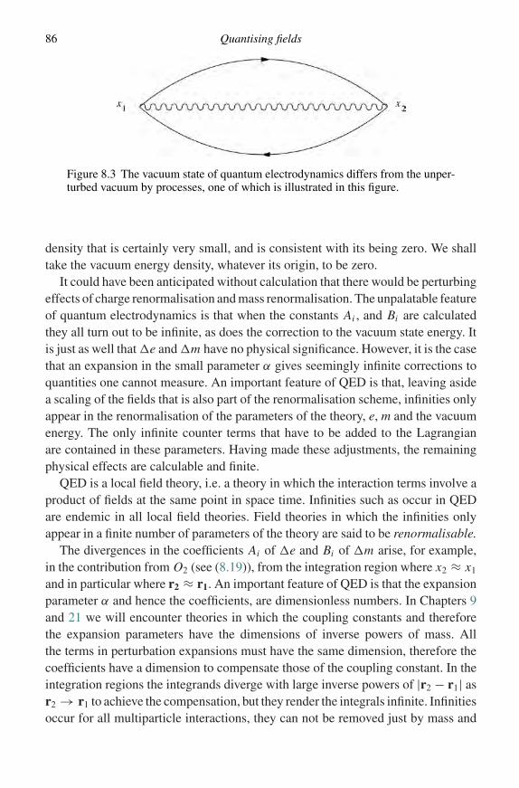
86 Quantising fields
Figure 8.3 The vacuum state of quantum electrodynamics differs from the unper-turbed vacuum by processes, one of which is illustrated in this figure.
density that is certainly very small, and is consistent with its being zero. We shalltake the vacuum energy density, whatever its origin, to be zero.
It could have been anticipated without calculation that there would be perturbingeffects of charge renormalisation and mass renormalisation. The unpalatable featureof quantum electrodynamics is that when the constants Ai , and Bi are calculatedthey all turn out to be infinite, as does the correction to the vacuum state energy. Itis just as well that e and m have no physical significance. However, it is the casethat an expansion in the small parameter α gives seemingly infinite corrections toquantities one cannot measure. An important feature of QED is that, leaving asidea scaling of the fields that is also part of the renormalisation scheme, infinities onlyappear in the renormalisation of the parameters of the theory, e, m and the vacuumenergy. The only infinite counter terms that have to be added to the Lagrangianare contained in these parameters. Having made these adjustments, the remainingphysical effects are calculable and finite.
QED is a local field theory, i.e. a theory in which the interaction terms involve aproduct of fields at the same point in space time. Infinities such as occur in QEDare endemic in all local field theories. Field theories in which the infinities onlyappear in a finite number of parameters of the theory are said to be renormalisable.
The divergences in the coefficients Ai of e and Bi of m arise, for example,in the contribution from O2 (see (8.19)), from the integration region where x2 ≈ x1
and in particular where r2 ≈ r1. An important feature of QED is that the expansionparameter α and hence the coefficients, are dimensionless numbers. In Chapters 9and 21 we will encounter theories in which the coupling constants and thereforethe expansion parameters have the dimensions of inverse powers of mass. Allthe terms in perturbation expansions must have the same dimension, therefore thecoefficients have a dimension to compensate those of the coupling constant. In theintegration regions the integrands diverge with large inverse powers of |r2 − r1| asr2 → r1 to achieve the compensation, but they render the integrals infinite. Infinitiesoccur for all multiparticle interactions, they can not be removed just by mass and

8.5 The magnetic moment of the electron 87
coupling constant renormalisation. Such theories are unrenormalisable, they cannot be taken seriously as quantum field theories.
8.5 The magnetic moment of the electron
We shall now illustrate the remarkable success of QED in calculating quantitiesof physical significance by giving an account of the calculation of the electron’smagnetic moment. In Chapter 7 we showed that the Dirac equation before secondquantisation implies that the electron carries a magnetic moment of magnitudeµB = eh/2m anti-aligned with its spin. The electron’s magnetic moment has beenmeasured with high precision: the experimental value µe is
µe = µB (1 + a)
where the ‘anomaly’ a = 0.001159 652 188 4(43) (Van Dyck et al., 1987).After second quantisation, the perturbative corrections to the Dirac value can be
calculated. The Dirac value is contained in the operator O1 of equation (8.16), andis associated with diagram (a) of Fig. 8.4. This lowest order calculation reproducesthe Dirac result µe = µB.
Since µB is the only combination of the parameters e, me and h which has thedimensions of magnetic moment, higher orders of perturbation theory will giveterms of the form
µe = µB(1 + αC1 + α2C2 + α3C3 + α4C4 + · · ·),where the Ci are dimensionless constants. To compare the theory with experimentwe use the 1986 adjusted value of the fine structure constant,
α−1 = 137.035 9979 (32) .
C1 is associated with diagram (b) of Fig. 8.4; the calculation gives C1 = 1/(2π ).Hence to this order
a = C1α = 0.001 161 409 74,
which agrees with experiment to within five significant figures.The next order correction, associated with diagrams (c) of Fig. 8.4, is
C2 = 1
π2
(197
144+ 3
4ζ (3)
)− 1
2ln 2 + 1
12
where ζ (z) is the Riemann zeta function. To this order,
a = 0.001 159 637 44,
in agreement to seven significant figures.

88 Quantising fields
Figure 8.4 Perturbation theory Feynman diagrams that represent contnbutions tothe electron magnetic moment. The anomalous moment, to order α2, comes fromcalculations associated with diagrams (b) and (c).

Problems 89
Calculations of higher orders of perturbation theory become rapidly moreintractable. Numerical estimates give C3 ≈ 0.03792, C4 ≈ −0.014. At this levelof accuracy, corrections have to be made for processes that come from other partsof the Standard Model, in particular from the muon. The most recent comprehensivecalculations (Kinoshita and Lindquist, 1990) give
a = 0.001 159 652 140 0 (41 + 53 + 271),
in agreement with experiment to ten significant figures. The largest error in thetheory is from the uncertainty in α−1.
Within its range of applicability, quantum electrodynamics provides an aston-ishingly exact model of Nature. One may have some confidence that the techniquesof renormalisation in perturbation theory are valid.
8.6 Quantisation in the Standard Model
In this chapter we have outlined the ‘canonical quantisation’ techniques that havebeen particularly successful in quantum electrodynamics. Many books have beenwritten on this subject, for example Itzykson and Zuber (1980); some will have tobe consulted if one is to be competent and confident in making detailed calcula-tions. However, many of the decay rates and cross-sections given in the followingchapters, which are needed to compare the predictions of the Standard Model withexperiment, are quite well approximated by the so-called ‘tree level’ of perturbationtheory. The tree-level diagrams have no closed loops (see Fig. 8.4(a)) and requireno renormalisation. It is a fortunate circumstance that in low orders of perturbationtheory these can be calculated quite easily.
The particles and forces of the weak and the strong interactions are also describedby local gauge field theories, which will be exhibited at the classical level in thechapters that follow. The quantisation procedures used in these extensions of QEDhave been most successfully pursued by the path integral method of quantisation(see, for example, Cheng and Li (1984)). Both the theory of the weak interactionand the theory of the strong interaction pose their own special problems, but theprinciples of gauge symmetry and renormalisability have been essential in theconstruction of the Standard Model as it is today.
Problems
8.1 A general two-particle state of scalar bosons (Section 8.1) can be written
|state〉 =∑k1,k2
f (k1, k2) a†k1 a†
k2|0〉,

90 Quantising fields
where, apart from normalisation, f (k1, k2) is any function of k1 and k2. (f can becalled the wave function of the state.)Show that this state may be written
|state〉 =∑k1,k2
g (k1, k2) a†k1 a†
k2|0〉
with g(k1, k2) = f (k1, k2) + f (k2, k1)/2, symmetric under the interchange oflabelling.
8.2 A general two-particle state of fermions can be written
|state〉 =∑
p1,ε1,p2,ε2
f (p1, ε1, p2, ε2) b†p1ε1
b†p2ε2
|0〉
where apart from normalisation f is any function of p1, ε1 and p2, ε2.Show that this state can also be written
|state〉 =∑
p1,ε1,p2,ε2
g (p1, ε1, p2, ε2) b†p1ε1
b†p2ε2
|0〉
with g(p1, ε1; p2, ε2) = f (p1, ε1; p2, ε2) − f (p2, ε2; p1, ε1/2, antisymmetric underthe interchange of labelling.
8.2 Use energy and momentum conservation to show that pair creation by a single photon,γ → e+ + e−, is impossible in free space.
8.3 The energy density of an electromagnetic field is given by equation (4.24). Show thatthe total electric field energy of a point charge q outside a sphere of radius R centredon the particle is
energy = q2/(8πR).
Note that this classical contribution to the particle rest energy is infinite in the limitR → 0.

9
The weak interaction: low energy phenomenology
In this chapter we review some of the early phenomenology of the weak interactionthat played an important guiding role in the construction of the Standard Model.The phenomenology discussed is insensitive to the very small effects of neutrinomass. These effects will be ignored.
9.1 Nuclear beta decay
In early investigations of nuclear physics, the existence of a ‘weak interaction’responsible for nuclear β decay was discerned. It was regarded as weak since themean lives of decays such as
179 F → 17
8 O + e+ + νe,
n → p + e− + νe,
are very long, minutes in these examples, compared with typical nuclear electro-magnetic decays, which have a mean life of ∼10−15s.
Nuclear physicists have by careful and ingenious experimentation establishedthe principal features of the weak interaction and the properties of the electronneutrino νe. To conserve electric charge the neutrino must be electrically neutral,and angular momentum is conserved if it is a Dirac spin 1
2 fermion. If the electronneutrino has a mass, it is certainly very small.
The surprising feature of the weak interaction, which was established experi-mentally in 1957 by Wu following a suggestion by Lee and Yang, is that it does notconserve parity. Nature is not ambidextrous. Indeed, parity is maximally violated,in that only the left-handed components of both the electron and neutrino fieldsparticipate in the interaction.
This phenomenon is clearly illustrated if one examines the longitudinal elec-tron polarisation of electrons produced in ‘allowed’ β decays. An electron ofnegative helicity − 1
2 and velocity v is in a left-handed state with probability
91

92 The weak interaction: low energy phenomenology
Figure 9.1 Measured degree of longitudinal polarisation P for allowed e− decays.(Data from Koks and Van Klinken (1976).)
12 [1 + (v/c)]; an electron of positive helicity + 1
2 is in a left-handed state withprobability + 1
2 [1 − (v/c)] (Section 6.5). In allowed nuclear β decays there are nonuclear factors that favour one helicity state over another, so that if only the left-handed component of the electron field participates in the interaction, the degreeof longitudinal polarisation of the emitted electron is
−1
2
(1 + v
c
)+ 1
2
(1 − v
c
)= −v
c.
For positrons, the probabilities are reversed (Section 6.5) and the longitudinal polar-isation of a positron emitted in an allowed β decay is +v/c. Data from several suchdecays are shown in Fig. 9.1.
A direct measurement of the helicities of neutrinos emitted in β decay is almostimpossible, but the helicities may be inferred from careful measurements of theangular momentum states of the participating nuclei. Within experimental error,only negative helicity neutrinos and positive helicity antineutrinos participate inthe weak interaction.
Nuclear β decays do not release sufficient energy to produce either of the twoother lepton families known to exist: muons and muon neutrinos, and tau leptons

9.2 Pion decay 93
Figure 9.2 π− → e− + ve. In this illustration the electron velocity is to the right,the antineutrino to the left, the spin directions are indicated Any orbital angularmomentum is out of the plane of the page (L = r × p) and since the total angularmomentum must be zero the spins have to be opposite.
and their partner neutrinos. We shall see in Chapter 13 that probably there are justthese three, e, µ, τ, lepton families. Each family seems to play a similar role inNature, an observation known as lepton universality. They differ only in the massesof the electrically charged leptons: me ≈ 0.511 MeV, mµ ≈ 106 MeV, mτ =1777 MeV.
9.2 Pion decay
An important example that illustrates both the left-handedness of the lepton fieldsparticipating in β decay and lepton universality is provided by the decay of thecharged pi mesons. These decays are common in the cosmic radiation and provideits principal component, muons, at ground level. Almost 100% of the pions decaythrough
π− → µ− + νµ, π+ → µ+ + νµ,
with a decay rate 1/τ (π → µνµ) = 2.53 × 10⁻¹⁴ MeV. The correspondingdecays to electrons have much smaller decay rates: 1/τ (π → eνe) = 1.23 ×10⁻⁴(1/τ (π → µνµ)).
The decay rate to electrons is suppressed because only the left-handed fields ofthe electron and neutrino take part. Consider the π− decay in a frame in whichthe pion is at rest (Fig. 9.2). The π− has zero spin, the antineutrino has positivehelicity. Hence to conserve angular momentum in this two-body decay the electronalso must have positive helicity. The probability of its being in the left-handed stateis 1
2 [1 − (ve/c)] = m2e/(m2
π + m2e) = 1.34 × 10⁻⁵ (Problem 9.1). The µ− decay is
similarly inhibited, but the muon’s much larger mass makes the factor less effective:12 [1 − (vµ/c)] = 0.36.
An effective interaction Lagrangian density that incorporates these featuresis
Lint = απ[ jµ∂µπ + jµ†∂µ†π], (9.1)

94 The weak interaction: low energy phenomenology
where
jµ = e†Lσ µveL + µ†Lσ µvµL + τ
†Lσ µvτL, (9.2)
and απ is an effective (real) coupling constant.π is a complex scalar field describing the charged π± mesons (Section 7.6).
π destroys negative pions, and creates positive pions. It is not a fundamental fieldof the Standard Model, since it ignores the internal structure of the pions. Thefour-vector e†Lσ µveL is the simplest Lorentz structure we can construct from thetwo left-handed spinor fields, eL, veL, belonging to the electron and its neutrino (seeProblem 5.3). Lepton universality is then incorporated in the model, the three leptonfamilies contributing in a similar way to the ‘current’ jµ; this structure survivesin the Standard Model. A Lorentz invariant Lint is obtained by taking the scalarproduct of jµ with ∂µ, and, finally, we make Lint real. Note that Lint is a ‘point’interaction: jµ and ∂µ are evaluated at the same point x in space-time. Since thepion is an extended object, this point interaction must be an approximation, not tobe taken too seriously.
An effective interaction Lagrangian is to be used only in low orders of perturba-tion theory. It is not suitable for calculating high order corrections. One should nottherefore demand high accuracy when comparing the results of a calculation withexperiment.
Using our Lint to lowest order, the partial decay rates for pions at rest are (Problem9.4)
1
τ(π → eνe)= α2
π
4π
(1 − υe
c
)p2
e Ee,1
τ(π → µνµ)= α2
π
4π
(1 − υµ
c
)p2
µEµ.
(9.3)
In these equations, Ee, Eµ and pe, pµ are the charged lepton’s energy and momen-tum, and are determined by energy and momentum conservation. The factorsp2
e Ee, p2µEµ come from the density of states factor in the expression for the transi-
tion probability (Problem 9.2). The factors (1 − υe/c) and (1 − υµ/c) are a conse-quence of the participation of left-handed fields only.
The ratio
τ (π → µνµ)
τ (π → eνe)= m2
e(m2π − m2
e)2
m2µ(m2
π − m2µ)2
= 1.28 × 10⁻⁴ (9.4)
(Problem 9.3). This lowest order calculation, which neglects the effects of non-locality and electromagnetic corrections, agrees well with the experimental valueof 1.23 × 10⁻⁴, and gives strong support for lepton universality.

9.3 Conservation of lepton number 95
The observations give 1/τ (π → eνe) = 3.11 × 10⁻¹⁸ MeV, 1/τ (π → µνµ) =2.53 × 10⁻¹⁴ MeV, from which we may estimate
απ = 2.09 × 10⁻⁹ MeV−1.
The smallness of απ reflects the weakness of the weak interaction.Although the pion does not have enough mass to decay to tau leptons, the effective
Lagrangian (9.1) also described the decays
τ+ → π+ + ντ, τ− → π− + ντ,
and in lowest order of perturbation theory, predicts
1
τ (τ → πντ)= α2
π
32πm3
τ[1 − (mπ/mτ)2]2. (9.5)
Using the estimate of απ from π± decay to calculate 1/τ (τ → πντ) provides afurther test of lepton universality: the predicted value 2.42 × 10⁻¹⁰ MeV comparesquite well with the experimental value, (2.6 ± 0.1) × 10−10 MeV.
9.3 Conservation of lepton number
In the model Lagrangian discussed so far, a single lepton can change only to anotherof the same family, and a lepton and antilepton of the same family can only becreated or destroyed together. There is thus a conservation law, the conservationof lepton number (antileptons being counted negatively), for each separate family,exemplified in the decays we have so far considered.
We saw in Section 7.1 that particle conservation follows from a U(1) symmetryof the Lagrangian, and it is interesting to see how this is accomplished with ourmodel Lagrangian. We have
L = Lfree + Lint
where, using Dirac spinors for the lepton fields,
Lfree = ∂µ†∂µ − m2π
†
+ ψe(γµi∂µ − me)ψe + νeγ
µi∂µνe
+ ψµ(γ µi∂µ − mµ)ψµ + νµγ µi∂µνµ
+ ψτ(γ µi∂µ − mτ)ψτ + ντγµi∂µντ,
Lint = απ[ jµ∂µπ + jµ†∂µ†π],
and, in terms of Dirac spinors, the current jµ of equation (9.2) can be written
jµ = ψeγµ 1
2(1 − γ 5)νe + ψµγ µ 1
2(1 − γ 5)νµ + ψτγ
µ 1
2(1 − γ 5)ντ. (9.6)

96 The weak interaction: low energy phenomenology
By itself, Lfree has seven U(1) symmetries: seven independent phases on theseven free fields. Including Lint reduces these to four, which can be written
ψe → eiβeiαee, νe → eiαeνe;
ψµ → eiβeiαµµ, νµ → eiαµνµ;
ψτ → eiβeiαττ, ντ → eiατντ;
π → eiβπ.
The phase factors αe, αµ, ατ are associated with the conserved lepton currents(Problem 9.6). If we require L to be invariant under a local gauge symmetry, withβ = β(x) arbitrarily space and time dependent, we are led to the introduction of theelectromagnetic field Aµ, as in Section 5.5. We shall see that not all these features ofour effective Lagrangian survive the introduction of neutrino mass into the StandardModel.
9.4 Muon decay
The analysis of the muon decays
µ− → e− + νe + νµ, µ+ → e+ + νe + νµ, (9.7)
has played a very important role in establishing the Standard Model. The decaysinvolve lepton fields only, so that the physics is not obscured by the phenomenologyof strong interaction fields as was our example of pion decay.
An effective Lagrangian density that describes the decays again couples theparticipating particles into currents. In fact all decays seen so far that involve justleptons are well described by the effective interaction Lagrangian density
Llepton = −2√
2G F gµν jµ jν†, (9.8)
with jµ again defined by (9.2) or (9.6). A similar form for nuclear β decay wasintroduced by Fermi, and GF is called the Fermi constant. The 2
√2 is a related
accident of history.The term in (9.8) that describes µ− decay is
L = −2√
2GFgµν
[e†Lσ µνeLν
†µLσ νµL
]. (9.9)
The most ready supply of muons comes from pion decays and these, as we haveseen, are almost 100% polarised. The interaction Lagrangian density (9.9) impliesa strong correlation between the angle θ made by the direction of the electron withthe direction of the muon spin, and the energy Ee of the electron. In the muon restframe, to lowest order of perturbation theory, and neglecting terms in (me/mµ)2,the decay rate into an angular interval dθ and energy interval dEe is (see Donoghue

9.4 Muon decay 97
et al. 1992, p. 138)
R(θ, Ee) dθ dEe = mµG2F
6π3
[(3
4mµ − Ee
)+ cos θ
(1
4mµ − Ee
)]E2
e dEe sin θdθ. (9.10)
Integrating (9.10) over θ and Ee gives the total decay rate for this process
1
τ(µ → eνeνµ)= m5
µG2F
192π3. (9.11)
The total muon decay rate, which includes also decays with photons in the finalstate, for example the decays
µ− → e− + γ + νe + νµ,
has been very accurately measured, giving
τµ = (2.19703 ± 0.00004) × 10−6 s.
A corresponding accurate theoretical expression that corrects (9.11) by includingterms in (me/mµ)2 and electromagnetic effects, gives
GF = 1.16639(2) × 10−5 GeV−2, (9.12)
which is the presently accepted value of this important constant.Further tests of lepton universality are provided by the decays
τ− → µ− + νµ + ντ, τ− → e− + νe + ντ,
and their charge conjugates. These, like muon decay, are described by appropriateterms in the interaction Lagrangian (9.8). Since both (me/mτ)2 and (mµ/mτ)2 aresmall, the first-order formula (9.11) with mµ replaced by mτ predicts these decayrates to be equal and ≈ 4 × 10⁻¹⁰ MeV. They are indeed so within experimentalerror. Also from this formula
τ (τ → eνeντ)
τ (µ → eνeνµ)≈
(mµ
mτ
)5
.
The ratio of the decay rates is 7.36 × 10⁻⁷ and the ratio of the fifth power of themasses is 7.43 × 10⁻⁷.
It should be noted that the coupling constant GF has the dimension of (mass)−2.The effective interaction (9.8) cannot be elevated into a quantum field interaction;see Section 8.4.

98 The weak interaction: low energy phenomenology
9.5 The interactions of muon neutrinos with electrons
In the 1960s, intense muon neutrino beams were engineered at Brookhaven andat CERN. Muon neutrinos (or antineutrinos) were produced as secondary particlesfrom the decay of π+ (or π−) mesons in flight. It was from the observation that theseneutrino beams produced almost exclusively muons rather than electrons, when ininteraction with a target, that the distinction between electron neutrinos and muonneutrinos was established.
The centre of mass energy√
s available in a collision of a neutrino with anelectron at rest is relatively small, because of the smallness of the electron mass. IfEν is the neutrino energy,
s = me(2Eν + me), (9.13)
(Problem 9.8). For example, if Eν = 30 GeV then s = (175 MeV)2, which willproduce no more than a muon. Most neutrino interactions will be with the atomicnuclei in the target. However, here we consider only the interactions with electrons.
The interaction
νµ + e− → µ− + νe
is included in the effective interaction Lagrangian density (9.8). In first-order per-turbation theory and averaging over electron polarisations, this Lagrangian predictsan isotropic differential cross-section in the centre of mass system:
dσ
d= G2
F
4π2
(s − m2
µ
)2
s, σtot = G2
F
π
(s − m2
µ
)2
s(9.14)
with s the square of the centre of mass energy. (See Okun 1982, p. 134.)At the low energies available experimentally, the cross-section appears to be
consistent with the theoretical form. The high energy structure is not easily exploredexperimentally, because of (9.13), but clearly the theoretical formulae becomeinadequate at high energies: the expressions (9.14) increase without limit as sincreases, and for a ‘point’ interaction this is inconsistent with unitarity. Nor isit possible to improve the expressions within this framework, since the effectiveLagrangian does not give a renormalisable theory.
The most significant result to come from the experiments on neutrino–electroninteractions was the observation of elastic scattering for both νµ and νµ:
νµ + e− → νµ + e−,
νµ + e− → νµ + e−,
with cross-sections of a magnitude similar to those for muon production. Such elas-tic scattering is not included in our Lint (though there are terms corresponding to

Problems 99
eνe → eνe and eνe → eνe). Thus another weak interaction must exist. The experi-mental investigation of this is difficult because of the smallness of the cross-sectionsat the available energies. We shall see from the Standard Model that the effectiveinteraction Lagrangian required is again of current–current form,
Lint = −G F√2
( jneutral)µ( jneutral)µ, (9.15)
where, in terms of Dirac spinors,
( jneutral)µ = νeγ
µ 1
2(1 − γ 5)νe + ψeγ
µ(cV − cAγ 5)ψe (9.16)
+ similar terms for the µ and τ lepton families,
and cV and cA are parameters. The current is called a neutral current because itdoes not induce a change of charge as do the currents (9.2). (Note that it will alsocontribute to the scattering eνe → eνe.)
Rewriting (9.16) with two-component spinors,
( jneutral)µ = (νeL)†σ µνeL + (cV + cA)e†Lσ µeL
+ (cV + cA)e†RσµeR + similar µ and τ terms. (9.17)
In this form it is evident that right-handed lepton fields as well as left-handedare involved in the neutral currents. The parameters cV and cA are related to theWeinberg angle θw, which appears in the Standard Model, as we shall see in Chapter12 (equation (12.24)). The subscripts V and A refer, respectively, to the vector andaxial vector nature of the terms in (9.16). (See Section 5.5.)
One might anticipate that neutral currents are also present in atomic physics,and indeed they are. However, their effects are hard to discern experimentally.For example, they induce parity violation in atoms, but at atomic energies theweak interaction gives a very small effect. Indeed the decay of an unstable nuclearor atomic system through the neutral current must always compete with fasterelectromagnetic decays, and for this reason neutral current decays in these systemshave never been observed.
Problems
9.1 In the decay of the π− at rest, π− → e− + νe, show that
1
2
(1 − υe
c
)= m 2
e
m 2π
+ m 2e
.

100 The weak interaction: low energy phenomenology
9.2 Show that the density of final states for the decay of Problem 9.1 is
ρ(E) = V
(2π)34πp2
edpe
dE
where V is the normalisation volume and
dpe
dE= Ee
mπ
.
9.3 Obtain the ratio of decay rates given by equation (9.4).
9.4 The term in Lint describing the decay π− → e− + νe is
Lint = απe†Lσ µνeL∂µπ.
Assume that this gives a corresponding term V(0) in the effective Hamiltonian,
V (0) = −απ
∫e†Lσ µνeL∂µπd3x.
(This assumption will be justified in Chapter 12.)The transition probability per unit time for the decay is to lowest order
2π|〈ep, ν p′ |V (0)|π−(rest)〉|2ρ(E)
where ρ(E) is given by Problem 9.2.Use the free field expansions given in equations (3.35) and (6.24), and Problem
6.5, to evaluate the matrix element above and hence verify equation (9.3).
9.5 Verify the equivalence of the expressions (9.2) and (9.6) for the current jµ.
9.6 Taking the effective Lagrangian of Section 9.3, show that the conserved current asso-ciated with the U(1) symmetry ψe → eiαψe, νe → eiανe, is the electron electron–neutrino current
jµ = ψeγµψe + νeγ
µνe.
Show that the conserved current associated with eiβ in the transformations (9.7)is
ψeγµψe + ψµγ µψµ + ψτγ
µψτ + i[(†∂µ − ∂µ†)
+ απ( jµ†† − jµ)].
Construct the Lagrangian density that results, when the electromagnetic field isintroduced by elevating the global U(1) symmetry of the phase factor eiβ into a localgauge symmetry.
9.7 Estimate GF from the expression (9.11) and the experimental lifetime τµ.
9.8 Using a suitable Lorentz invariant, obtain equation (9.13).

Problems 101
9.9 Pick out the term in the effective Lagrangian density (9.8) that contributes to thescattering
e− + νe → e− + νe,
and the term in (9.15) that contributes to the scattering
e− + νµ → e− + νµ.
9.10 The K− is like the π−, but with an s quark replacing the d. An effective inter-action with leptons is similar in form to equation (9.1), with K replacing π
and αK replacing απ. Use the analogue of equation (9.4) to estimate the ratioτ (K → µνµ)/τ (K → eνe), and compare with the observed value (2.44 ± 0.1) ×10−5 (mK = 493.68 MeV).
The mean life τ (K− → µ−νµ) is measured to be 1.948 × 10⁻⁸ s. EstimateαK/απ.
9.11 Obtain the decay rate (9.5).

10
Symmetry breaking in model theories
In Chapter 9, ‘effective’ weak interaction Lagrangian densities were constructed.When used in low orders of perturbation theory, these account well for the observedphenomena at low energies. Difficulties arise in higher order perturbation theory, asthey do in quantum electrodynamics. There is, however, an important difference: ithas been proved that these effective Lagrangian theories cannot be renormalised andthey are therefore unsatisfactory. Furthermore, at higher energies new phenomenaappear, and it is now well established experimentally that the weak interaction ismediated by the W+, W− and Z bosons. How are these particles to be incorporated ina theory of the weak interaction that can be renormalised, and which has the sameseeming inevitability as QED? The answer lies in the Weinberg–Salam unifiedtheory of the electromagnetic and weak interactions. As an introduction to theWeinberg–Salam theory we shall in this chapter consider ‘model’ theories, themathematics of which is fairly simple, but which contain the basic ideas we shallneed.
10.1 Global symmetry breaking and Goldstone bosons
A possible Lagrangian density for a complex scalar field = (φ1 + iφ2)/√
2 is
L = ∂µ†∂µ − m2† (10.1)
(cf. equation (3.32)).In this expression (∂†/∂t)(∂/∂t) can be regarded as the kinetic energy density
and ∇† · ∇ + m2† as the potential energy density (see Section 3.3). If isconstant, independent of space and time, the only contribution to the energy ism2†. Since m2 is positive this will be a minimum when φ1 = φ2 = 0. Thus = 0 corresponds to the ‘vacuum’ state. Consider now the Lagrangian densityobtained by changing the sign in front of m2. This would be unstable: the potential
102

10.1 Global symmetry breaking: Goldstone bosons 103
Figure 10.1 Plot of V = (m2/2φ20)[∗ − φ2
0]2 as a function of ||; is here aclassical field.
energy density is then unbounded below. Stability can be restored by introducinga term (m2/2φ2
0)(†)2 where φ20 is another (real) parameter. For convenience we
add a constant term m2φ20/2, and then
L = ∂µ†∂µ − V (†)
where
V (†) = m2
2φ20
[† − φ2
0
]2. (10.2)
The form of V is shown in Fig. (10.1). The minimum field energy is now obtainedwith constant independent of space and time, but such that † = ||2 = φ2
0 .Such a field is not unique but is defined by a point on the circle || = φ0 in thestate space (φ1, φ2), so that the number of possible vacuum states is infinite.
An analogy with magnetism is helpful. The Hamiltonian describing aHeisenberg ferromagnet has rotational symmetry: all directions in space are equiv-alent. However, in its ground state a ferromagnet is magnetised in some particulardirection, which is not determined within the theory, and the rotational symmetryis lost. This is an example of spontaneous symmetry breaking.

104 Symmetry breaking in model theories
The Lagrangian density (10.2) has a ‘global’ U(1) symmetry: → ′ =e−iα, L → L′ = L, for any real α. Equivalently,
φ′1 = φ1 cos α + φ2 sin α,
φ′2 = − φ1 sin α + φ2 cos α.
The transformation rotates the state round a circle ||2 = constant in the state space(φ1, φ2). If we pick out the particular direction in (φ1, φ2) space for which is real,and take the vacuum state to be (φ0, 0), we break the U(1) symmetry.
Expanding about this ground state (φ0, 0), we put = φ0 + (1/√
2)(χ + iψ).The Lagrangian density becomes
L = 1
2∂µχ∂µχ + 1
2∂µψ∂µψ − m2
2φ20
[√2φ0χ + χ2
2+ ψ2
2
]2
. (10.3)
After breaking the U(1) symmetry we must interpret the new fields. (In much thesame way, the excited states of a ferromagnet cannot be discussed until the spatialsymmetry has been broken.) In place of the complex field , we have two coupledscalar real fields χ and ψ . We write
L = Lfree + Lint
where
Lfree = 1
2∂µχ∂µχ − m2χ2 + 1
2∂µψ∂µψ. (10.4)
Lfree represents free particle fields, and contains all the terms in L that are quadraticin the fields. For classical fields and small oscillations, these terms dominate. Therest of the Lagrangian density, Lint, corresponds to interactions between the freeparticles and higher order corrections to their motion.
There is a quadratic term −m2χ2 in (10.4), so that the χ field corresponds toa scalar spin-zero particle of mass
√2m (by comparison with (3.18)). In the case
of the ψ field there is no such quadratic term: the corresponding scalar spin-zeroparticle is therefore massless. The massless particles that always arise as a result ofglobal symmetry breaking are called Goldstone bosons.
10.2 Local symmetry breaking and the Higgs boson
We now generalise further, and construct a Lagrangian density that is invariantunder a local U(1) gauge transformation,
→ ′ = e−iqθ,

10.2 Local symmetry breaking and the Higgs boson 105
where θ = θ (x) may be space and time dependent. This requires the introductionof a (massless) gauge field Aµ, as in Section 7.5, and we take
L = [(∂µ − iq Aµ)†][(∂µ + iq Aµ)] − 1
4Fµν Fµν − V (†), (10.5)
where Fµν = ∂µ Aν − ∂ν Aµ, and again
V (†) = m2
2φ20
[† − φ2
0
]2.
L is invariant under the local gauge transformation
(x) → ′(x) = e−iqθ(x), Aµ(x) → A′µ(x) = Aµ(x) + ∂µθ (x).
A minimum field energy is obtained when the fields Aµ vanish, and is constant,defined by a point on the circle || = φ0. Any gauge transformation on this fieldconfiguration is also a minimum. Again we have an infinity of vacuum states.
Given (x), we can always choose θ (x) so that the field ′(x) = e−iqθ(x) isreal. This breaks the symmetry, since we are no longer free to make further gaugetransformations.
Putting ′(x) = φ0 + h(x)/√
2, where h(x) is real, gives
L = [(∂µ − iq A′µ)(φ0 + h/
√2)][(∂µ + iq A′µ)(φ0 + h/
√2)]
− 1
4F ′
µν F ′µν − m2
2φ20
[√2φ0h + 1
2h2
]2
. (10.6)
For clarity, we again separate this into
L = Lfree + Lint
where, dropping the primes on the gauge field,
Lfree = 1
2∂µh∂µh − m2h2 − 1
4Fµν Fµν + q2φ2
0 Aµ Aµ,
Lint = q2 Aµ Aµ
(√2φ0h + 1
2h2
)− m2h2
2φ20
(√2φ0h + 1
4h2
).
(10.7)
Before symmetry breaking, we had a complex scalar field = (φ1 + iφ2)/√
2,and a massless vector field with two polarisation states (Section 4.4). In Lfree wehave a single scalar field h(x) corresponding to a spinless boson of mass
√2m,
and a vector field Aµ, corresponding to a vector boson of mass√
2qφ0, with threeindependent components (Section 4.9).
This mechanism for introducing mass into a theory was invented by Higgs (1964)and others (for example Anderson, 1963), and the particle corresponding to the fieldh(x) is called a Higgs boson. As a consequence of local symmetry breaking the gauge

106 Symmetry breaking in model theories
field acquires a mass, and the massless spin-zero Goldstone boson that appearedin our example of global symmetry breaking in Section 10.1 is replaced by thelongitudinal polarised state of this massive spin one boson.
In the Weinberg and Salam ‘electroweak’ theory, the masses of the W± andZ particles arise as a result of symmetry breaking. The resulting theory can berenormalised, whereas the phenomenological theory of Chapter 9 cannot be renor-malised. The form of V (†) that has been introduced in this chapter appears alsoin the electroweak theory. It may seem a somewhat arbitrary feature. However, itcan be shown to be the most general form that can be renormalised.
Problems
10.1 What interaction term in the model Lagrangian density (10.3) allows the massiveboson to decay into two Goldstone bosons? Show that the decay rate in lowest orderperturbation theory is
1
τ (χ → ψψ)= mχ
128π
(mχ
φ0
)2
.
10.2 Show that with the model Lagrangian density (10.7), the vector boson would bestable, but if the coupling constant q < m/(2φ0) the scalar boson would decay intotwo vector bosons.

11
Massive gauge fields
In the preceding chapter (Section 10.2), we set up a simple Lorentz invariantLagrangian density, which we required to be also invariant under a local U(1)transformation. This requirement leads to the introduction of a ‘gauge field’ Aµ.The system has a degenerate ground state. Breaking the local symmetry results inthe appearance of a vector field carrying mass, together with a scalar Higgs fieldalso carrying mass. The motivation for introducing mass in this way is that thesubsequent quantum theory can be renormalised. In this chapter we apply the sameidea to a more complicated Lagrangian, which will turn out to have remarkablephysical significance.
11.1 SU(2) symmetry
As a further generalisation, which is basic to the Standard Model, we shall constructa Lagrangian density that is invariant under a local SU(2) transformation as well asa local U(1) transformation. The idea was first explored by Yang and Mills (1954).We introduce a two-component field
=(
A
B
), (11.1)
where now A and B are both complex scalar fields,
A = φ1 + iφ2, B = φ3 + iφ4,
giving, in total, four real fields.If e−iθ is any element of the group U(1) and U is any element of the group SU(2)
(discussed in Appendix B), so that U†U = UU† = 1, we require the Lagrangiandensity to be invariant under the U(1) × SU(2) transformation
→ ′ = e−iθU. (11.2)
107

108 Massive gauge fields
A simple Lagrangian density that has a global U(1) × SU(2) symmetry is
L = ∂µ†∂µ − V (†). (11.3)
In terms of the real fields,
† = ∗AA + ∗
BB = φ21 + φ2
2 + φ23 + φ2
4,
∂µ†∂µ = ∂µφ1∂µφ1 + ∂µφ2∂
µφ2 + ∂µφ3∂µφ3 + ∂µφ4∂
µφ4.
If V (†) = m2†, this Lagrangian density corresponds to four independentfree scalar fields, all with the same mass m (cf. (3.18)).
In the Standard Model, the U(1) and SU(2) global symmetries are promoted tolocal symmetries. The U(1) transformation may be written
→ ′ = e−iθ = exp(−iθτ 0), (11.4a)
where in this context we write τ 0 for the unit matrix
τ 0 =(
1 00 1
).
For this to become a local symmetry, we must introduce a vector gauge field Bµ(x)τ 0
with the transformation law
Bµ(x) → B ′µ(x) = Bµ(x) + (2/g1)∂µθ, (11.4b)
and make the replacement
i∂µ → i∂µ − (g1/2)Bµ,
as in Chapter 7. Here the constant g1 is a dimensionless parameter of the theory,and the factor 2 follows convention.
Any element of SU(2) can be written in the form
U = exp(−iαkτ k) (11.5)
where the αk are three real numbers and the τ k are the three generators of the groupSU(2). The τ k are identical to the Pauli spin matrices:
τ 1 =(
0 11 0
), τ 2 =
(0 −ii 0
), τ 3 =
(1 00 −1
).
For the global SU(2) symmetry to be made into a local SU(2) symmetry, with U =U(x) dependent on space and time coordinates, we must introduce a vector gaugefield Wµ
k(x) for each generator τ k . The transformation law for the matrices
Wµ(x) = Wµk(x)τ k

11.2 The gauge fields 109
is
Wµ(x) → W′µ(x) = U(x)Wµ(x)U†(x) + (2i/g2)(∂µU(x))U†(x), (11.6)
which is a generalisation of (11.4). Here g2 is another dimensionless parameter ofthe theory.
Note that the matrices
Wµ(x) =(
W 3µ
W 1µ + iW 2
µ
W 1µ − iW 2
µ
−W 3µ
)(11.7)
are Hermitian and have zero trace. These properties are preserved by the transfor-mation (11.6) as is clearly necessary (Problem 11.1). A global SU(2) transformationW′
µ= UWµU† corresponds to a rotation of the vectors Wµk in the three-dimensional
‘weak isospin’ space defined by the generators τ k . (See Appendix B.)Finally we define
Dµ = [∂µ + (ig1/2)Bµ + (ig2/2)Wµ]. (11.8a)
It is straightforward to show
D′µ′ = [∂µ + (ig1/2)B ′
µ + (ig2/2)W′µ]′ = e−iθUDµ,
where
′ = e−iθU. (11.8b)
Hence the locally gauge invariant Lagrangian density corresponding to (11.3) is
L = (Dµ)†Dµ − V (†). (11.9)
L is also invariant under Lorentz transformations if we require Bµ and Wµ totransform as covariant four-vectors.
11.2 The gauge fields
In the case of the gauge field Bµ, we define the field strength tensor Bµν by
Bµν = ∂µ Bν − ∂ν Bµ, (11.10)
and take the dynamical contribution to the Lagrangian density to be −(1/4) Bµν Bµν ,as in Section 4.2.

110 Massive gauge fields
There are additional complications in introducing the field strength tensors forthe gauge fields Wµ, stemming from the non-Abelian nature of the group SU(2).The field strength tensor must be taken to be
Wµν = [∂µ + (ig2/2)Wµ]Wν − [∂ν + (ig2/2)Wν]Wµ. (11.11)
Under an SU(2) transformation, Wµ → W′µ, given by (11.6), it is straightforward,
if tedious, to show that
Wµν → W′µν
= UWµνU†. (11.12)
In verifying this result, note that, since UU† = 1,
U(∂µU†) + (∂µU)U† = 0.
The complicated definition of Wµν given by (11.11) is necessary in order to achievethe simple transformation property (11.12).
We then take the total dynamical contribution to the Lagrangian density associ-ated with the gauge fields to be
Ldyn = −1
4Bµν Bµν − 1
8Tr(WµνWµν). (11.13)
Using (11.12) and the cyclic invariance of the trace, we can see that Ldyn is invariantunder a local SU(2) transformation.
Using the results [τ 2, τ 3] = 2iτ 1, etc., the matrix Wµν may be written
Wµν = W iµντ
i (11.14)
where
W 1µν
= ∂µW 1ν − ∂νW 1
µ − g2(W 2
µW 3ν − W 2
ν W 3µ
), (11.15a)
W 2µν
= ∂µW 2ν − ∂νW 2
µ − g2(W 3
µW 1ν − W 3
ν W 1µ
), (11.15b)
W 3µν
= ∂µW 3ν − ∂νW 3
µ − g2(W 1
µW 2ν − W 1
ν W 2µ
). (11.15c)
Since Tr(τ i )2 = 2, and Tr(τ iτ j ) = 0, i = j , we can use (11.14) to express theLagrangian density in the more reassuring form:
Ldyn = −1
4Bµν Bµν −
3∑i=1
1
4W i
µνW iµν. (11.16)
We shall see, later in this chapter, that the fields W 1µ and W 2
µ are electricallycharged, and it is convenient to define here the complex combinations
W +µ = (
W 1µ − iW 2
µ
)/√
2, W −µ = (
W 1µ + iW 2
µ
)/√
2. (11.17)

11.3 Breaking the SU(2)symmetry 111
Note that the field W −µ is the complex conjugate of the field W +
µ . We also define
W +µν = (
W 1µν − iW 2
µν
)/√
2
= (∂µ + ig2W 3
µ
)W +
ν − (∂ν + ig2W 3
ν
)W +
µ (11.18)
using (11.15a) and (11.15b). W −µν is defined similarly.
We can also write (11.15c) as
W 3µν = ∂µW 3
ν − ∂νW 3µ − ig2
(W −
µ W +ν − W −
ν W +µ
)(11.19)
and (11.16) becomes
Ldyn = −1
4Bµν Bµν − 1
4W 3
µνW 3µν − 1
2W −
µνW +µν. (11.20)
11.3 Breaking the SU(2) symmetry
As in equation (10.2) we take V (†) to be
V (†) = m2
2φ20
[(†) − φ2
0
]2
= m2
2φ20
[φ2
1 + φ22 + φ2
3 + φ24 − φ2
0
]2(11.21)
where φ0 is a fixed parameter that is the analogue of (10.2). With this expressionfor V, the vacuum state of our system is degenerate in the four-dimensional spaceof the scalar fields. We now break the SU(2) symmetry. At our disposal we have thethree real parameters αk(x) that specify an element of SU(2). We use this freedomto adopt a gauge in which for any field configuration A = 0 (two conditions) andB is real (one condition). The ground state is then
ground =(
0φ0
), (11.22)
and excited states are of the form
=(
0φ0 + h(x)/
√2
), (11.23)
where the field h(x) is real.A local U(1) symmetry remains: the fields (11.23) are unchanged by a U(1) ×
SU(2) transformation of the form
e−iθ/2
(e−iθ/2 00 eiθ/2
)=
(e−iθ 00 1
). (11.24)

112 Massive gauge fields
Such matrices give a 2 × 2 matrix representation of the group U(1). This residualsymmetry will turn out to be the U(1) symmetry of electromagnetism.
We wish to express L (equation (11.9)) in terms of the field h(x). We have from(11.21)
V ( †) = m2h2 + m2h3
√2φ0
+ m2h4
8φ20
= V (h),
and from (11.8a) and (11.7)
Dµ =(
0∂µh/
√2
)+ ig1
2
(0Bµ(φ0 + h/
√2)
)+ ig2
2
(√2W +
µ (φ0 + h/√
2)−W 3
µ(φ0 + h/√
2)
).
Multiplying (Dµ)† by Dµ, we find
L = 1
2∂µh∂µh + g2
2
2W −
µ W +µ(φ0 + h/√
2)2
+[
g22
4W 3
µW 3µ − g1g2
2W 3
µ Bµ + g21
4Bµ Bµ
](φ0 + h/
√2)2 − V (h)
= 1
2∂µh∂µh + g2
2
2W −
µ W +µ(φ0 + h/√
2)2
+ 1
4
(g2
1 + g22
)ZµZµ(φ0 + h/
√2)2 − V (h). (11.25)
We have written
Zµ = W 3µ cos θw − Bµ sin θw, (11.26)
where
cos θw = g2(g2
1 + g22
)1/2 , sin θw = g1(g2
1 + g22
)1/2 . (11.27)
θw is called the Weinberg angle.Along with the field Zµ, we define the orthogonal combination
Aµ = W 3µ sin θw + Bµ cos θw. (11.28)
Equations (11.26) and (11.28) correspond to a rotation of axes in (Bµ, W 3µ) space.
The rotation can be inverted to give
Bµ = Aµ cos θw − Zµ sin θw,
W 3µ = Aµ sin θw + Zµ cos θw.
(11.29)
Substituting in (11.10) and (11.19) gives
Bµν = Aµν cos θw − Zµν sin θw,
W 3µν = Aµν sin θw + Zµν cos θw − ig2
(W −
µ W +ν − W −
ν W +µ
),

11.4 Identification of the fields 113
where
Aµν = ∂µ Aν − ∂ν Aµ (Aµν is the Fµν of Chapter 4)
and
Zµν = ∂µZν − ∂v Zµ. (11.30)
11.4 Identification of the fields
We are now in a position to rearrange the terms in the full Lagrangian densityL = L + Ldyn to reveal its physical content. In Ldyn (equation (11.20)) we use(11.29) and (11.30) to express the field Bµ and W 3
µ in terms of the fields Aµ andZµ, and then we may write
L = L1 + L2,
where
L1 = 1
2∂µh∂µh − m2h2
− 1
4Zµν Zµν + 1
4φ2
0
(g2
1 + g22
)ZµZµ
− 1
4Aµν Aµν
− 1
2
[(DµW +
ν
)∗ − (DνW +
µ
)∗][DµW +ν − DνW +µ] + 1
2g2
2φ20W −
µ W +µ,
(11.31)
and DµW +ν = (∂µ + ig2 sin θw Aµ)W +
ν .L1 is relatively simple: you will recognise it as the Lagrangian density for a
free massive neutral scalar boson field h(x), a free massive neutral vector bosonfield Zµ(x), and a pair of massive charged vector boson fields W +
µ (x) and W −µ (x),
interacting with the electromagnetic field Aµ(x).L2 is the sum of the remaining interaction terms. As the patient reader may
verify,
L2 =(
1
4h2 + 1√
2hφ0
) (g2
2 W −µ W +µ + 1
2
(g2
1 + g22
)ZµZµ
)− m2h3
√2φ0
− m2h4
8φ20
+ g22
4
(W −
µ W +ν − W −
ν W +µ
)(W −µW +ν − W −νW +µ)
+ ig2
2(Aµν sin θw + Zµν cos θw)(W −µW +ν − W −νW +µ)
− g22 cos2 θw(ZµZµW −
ν W +ν − ZµZ νW −ν W +µ)

114 Massive gauge fields
+ ig2
2cos θw[(ZµW −
ν − ZνW −µ )(DµW +ν − DνW +µ)
− (ZµW +
ν − ZνW +µ
)(DµW +ν)∗ − (DνW +µ)∗)]. (11.32)
Most of the U(1) × SU(2) symmetry with which we began has been lost onsymmetry breaking. In particular, no trace of the original SU(2) symmetry is to beseen in the interactions described by L2. Nevertheless it is precisely this complicatedset of interactions that makes the theory renormalisable, as it would be if thesymmetry were not broken.
We identify the three vector fields, W +µ , W −
µ , Zµ, with the mediators of theweak interaction, the W +, W −, Z particles, which, subsequent to the theory, werediscovered experimentally. The masses are (Particle Data Group, 2004)
Mw = 80.425 ± 0.038 GeV, (11.33)
Mz = 91.1876 ± 0.0021GeV. (11.34)
From (11.31) and Section 4.9, we identify
φ0g2/√
2 = Mw, (11.35)
φ0(g2
1 + g22
)1/2/√
2 = Mz. (11.36)
Then, from (11.27), and neglecting quantum corrections to the mass ratio,
cos θw = Mw/Mz = 0.8810 ± 0.0016. (11.37a)
It is usual to quote the value of sin2 θw, which will appear in later calculations.The estimate above would suggest
sin2 θw = 0.23120 ± 0.00015.
The uncertainty arises mainly from uncertainty in Mw. Other ways of estimatingsin2 θw exist and the accepted value (in 1996) was
sin2 θw = 0.2315 ± 0.0004. (11.37b)
We shall adopt this value in subsequent calculations.The W± bosons are found experimentally to carry charge ±e. In (11.31) the
gauge derivative is
DµWν+ = (∂µ + ig2 sin θw Aµ)Wν
+,
so that from the coupling to the electromagnetic field Aµ and (11.27) we canidentify
e = g2 sin θw = g1 cos θw. (11.38)

Problems 115
The fields W 1µ, W 2
µ, and Zµ have free field expansions similar to (4.15) but withthree polarisation states (see Section 4.9). As a quantum field W +
µ destroys W+
bosons and creates W− bosons; W −µ destroys W− bosons and creates W+ bosons.
There remains the scalar Higgs field h(x). The vacuum state expectation valueφ0 of the Higgs field is, from (11.35),
φ0 =√
2Mw
g2=
√2Mw sin θw
e= 180 GeV. (11.39)
The only parameter not fixed from experiment is the mass MH = √2m of the
Higgs boson. No Higgs boson has yet been identified experimentally, thoughits existence is, apparently, an essential part of the Standard Model. The fail-ure so far of experimental searches to find the Higgs boson suggests MH >
64 GeV. Recent experimental and theoretical studies suggest an MH close to thislimit.
The requirements of U(1) and SU(2) symmetry, followed by SU(2) symmetrybreaking, have generated the electromagnetic field, the massive vector W± and Zboson fields, and the scalar Higgs field, in a remarkably economical way. In the nextchapter, we add lepton fermion fields to these boson fields, to obtain the richnessof the Weinberg–Salam electroweak theory.
Problems
11.1 Show that the W′µ defined by (11.6) are Hermitian and have zero trace. (Use the
expression (B.9) of Appendix B: U= cos αI+i sin α(α · τ ).)
11.2 Verify that the expressions (11.13) and (11.16) for Ldyn are equivalent.
11.3 Verify that the last two terms on the right-hand side of (11.31) correspond to a pairof massive charged vector boson fields.
11.4 Show that the Higgs boson can decay to two photons, in the third order of perturbationtheory. Draw the appropriate Feynman graph.
11.5 Under an SU(2) transformation, → ′ where(′
A
′B
)= U
(A
B
).
Using (B.9), show that τ 2U ∗ = Uτ 2. Hence show that(′∗
B
−′∗A
)= U
(∗
B
−∗A
).

116 Massive gauge fields
11.6 Show that the SU(2) matrix U = eiτα with α = α(sin φ, cos φ, 0) is
U =(
cos α eiφ sin α
−e−iφ sin α cos α
).
Show that under the SU(2) transformation ′ = U, the two-component complexfield
=(
A
B
)=
(aeiδ
beiγ
)can be put in the form
′ =(
′A
′B
)=
(0
eiγ√
a2 + b2
),
taking φ = (δ − γ ) and α = − tan−1(a/b). Show that ′ can then be put in thestandard form (11.23) by a further SU(2) transformation with α = γ (0, 0, 1).

12
The Weinberg–Salam electroweak theory for leptons
We shall now couple the lepton fields to all the gauge boson fields: the electromag-netic field, the W + and W − fields, and the Z field. We know that at low energiesthe theory must reproduce the phenomenology of Chapter 9. This considerationand the principles of U (1) × SU (2) local gauge symmetry determine the couplingsuniquely.
We have seen how the Higgs mechanism gives mass to the W± and Z bosons. Togive mass to the charged leptons: the electron, the muon, the tau, they too must becoupled to the Higgs field. We shall finally arrive at the Weinberg–Salam unifiedtheory of the electroweak interaction.
12.1 Lepton doublets and the Weinberg–Salam theory
We shall first construct a Lagrangian density for lepton fields that is invariant underU(1) and SU(2) transformations. The left-handed electron spinor eL and the electronneutrino spinor νeL are put together in an SU(2) doublet, like the Higgs fields inequation (11.1),
L =(
νeL
eL
)=
(LA
LB
). (12.1)
We are now again specialising our notation; two-component left-handed and right-handed spinors were denoted by ψL and ψR, respectively, in Chapter 6. Under anSU(2) transformation, this doublet transforms in exactly the same way as the Higgsdoublet:
L → L′ = UL. (12.2)
Since SU(2) transformations mix the two spinor fields making up the doublet,to maintain Lorentz invariance only fields with the same Lorentz transformationproperties can be combined together into a doublet.
117

118 Weinberg–Salam electroweak theory for leptons
From the phenomenology of Chapter 9 the right-handed lepton fields donot couple to the W boson field so that eR and νeR are invariant under SU(2)transformations:
eR → e′R = eR. νeR → ν ′
eR = νeR. (12.3)
To be consistent with the transformation rule (12.2), all SU(2) gauge derivativesmust be of the same form, ∂µ + i(g2/2)Wµ, where g2sin θw=e, as in (11.8) and(11.38). This is a consequence of the non-Abelian nature of the group SU(2).However, there is no similar constraint on the coupling constant to the U(1) gaugefield Bµ. (See Problem 12.1.) We may take
DµL = [∂µ+i(g2/2)Wµ+i(g′/2)Bµ)]L, (12.4)
where g′ remains at our disposal. We must choose g′ so that the neutrino is neutraland the electron has charge −e. The terms in DµL which couple to the electromag-netic field Aµ are linear combinations of W 3
µ and Bµ. Using (11.7) and (11.29) theterms in Aµ are(
∂µ + i(g2/2) sin θw + i(g′/2) cos θwAµ, 00, ∂µ + −i(g2/2) sin θw + i(g′/2) cos θwAµ
) (νeL
eL
).
The gauge derivatives ∂µνeL and (∂µ − ieAµ)eL which leave the neutrino electricallyneutral but impart electric charge −e to eL, are obtained with the choice
g′ cos θw = −g2 sin θw = −e.
The complete gauge derivative of the left-handed fields is then
DµL =(
∂µ + i(e/ sin 2θw)Zµ, ie/(√
2 sin θw)W +µ
ie/(√
2 sin θw)W −µ , ∂µ − ieAµ − ie cot(2 θw)Zµ
) (νeL
eL
)(12.5)
where we have used (11.7), (11.17) and (11.29).The gauge derivative of eR must be of the form
DµeR= [∂µ+i(g′′/2)Bµ]eR. (12.6a)
Since the electron has charge −e we take g′′ = −2e/cos θw = −2g1, (see (11.38))so that, using (11.29) again,
DµeR= [(∂µ−ieAµ) + ie tan θw Zµ]eR. (12.6b)
With g′′ = −2g1 and g′ = −g1, it can easily be checked that, under a localU (1) × SU (2) transformation
L → L′ = eiθ (x)U(x)L,
eR → e′R = e2iθ (x)eR,

12.1 Lepton doublets and the Weinberg–Salam theory 119
the gauge derivatives satisfy
Dµ′L′ = (∂µ + i(g2/2)Wµ
′ + i(g′/2)Bµ′)L′ = eiθUDµL
Dµ′eR
′ = (∂µ + i(g′′/2)Bµ′)eR
′ = e2iθDµeR,
where the fields Bµ and Wµ transform as in (11.4b) and (11.6).We can now construct a gauge invariant and Lorentz invariant expression for the
dynamical part of the Lagrangian density for the electron and the electron neutrino:
Ledyn = L†σ µiDµL + e†
RσµiDµeR + ν+eRσµi∂µνeR. (12.7)
The gauge invariance follows from our construction of the gauge derivatives, andthe Lorentz invariance from the spinor properties set out in Section 5.4. (Rememberthat the σµ matrices act on the spinor indices, whereas the SU(2) transformationacts independently on the components of the doublet of spinor fields.) Note thatbesides the interaction with the electromagnetic field we have fully determined,from the factor DµL, all the interactions with the heavy vector bosons.
Finally, we must give mass to the charged leptons. A gauge and Lorentz invariantcontribution to the Lagrangian density that will impart mass to the electron but leavethe neutrino massless is (neutrino mass will be introduced in Chapter 19)
Lemass = −ce[(L†)eR + e†R(†L)]
= −ce[(ν†LA + e†LB)eR + e†R(†
AνL + †BeL)],
(12.8)
where is the Higgs doublet field and ce is a dimensionless coupling constant.After symmetry breaking (see (11.23)), Le
mass becomes
Lemass = −ceφ0(e†LeR + e†ReL) − ceh√
2
(e†LeR + e†ReL
). (12.9)
Comparing this with the Dirac Lagrangian density (5.12), we identify ceφ0 withthe electron mass me. Introducing mass by following the principles of symmetryhas left us no option but to introduce an interaction between the electron field andthe Higgs field h(x). Hence the coupling constant to the Higgs field is
ce√2
= me√2φ0
= 2.01 × 10⁻⁶ (12.10)
(using (11.39)). It is just as well that ce is small: we do not want this term to upsetthe calculations of QED!
The total Lagrangian density Le for the electron and its neutrino is given by(12.7) and (12.8):
Le = Ledyn + Le
mass. (12.11)

120 Weinberg–Salam electroweak theory for leptons
From Le we can pick out the terms
Le
Dirac = ν†eLσ µi(∂µνeL)+e†Lσ µi(∂µ − ieAµ)eL + ν
†eRσµi∂µνeR
+ e†Rσµi(∂µ − ieAµ)eR − me(e†LeR + e†ReL
),
(12.12)
which correspond to the expressions we found in Chapter 6 and Chapter 7 for aDirac massless neutrino, and a Dirac electron of mass me and charge −e in anelectromagnetic field.
The Lagrangian densities Lµ and Lτ for the muon and tau leptons and their neu-trinos differ from (12.11) only in their mass parameters and, hence, their couplingsto the Higgs field:
cµ√2
= mµ√2φ0
= 4.15 × 10⁻⁴,cτ√
2= mτ√
2φ0
= 6.98 × 10⁻³. (12.13)
The coupling constant g2 of the SU(2) gauge theory, or, equivalently, the Weinbergangle θw (see (11.38)), which determines the coupling to the W ± and Z fields, mustbe the same for all leptons, a feature of the theory that is forced on us by the SU(2)group, and that is known as lepton universality.
The complete Lagrangian density Lws of the Weinberg–Salam theory (Wein-berg, 1967; Salam, 1968) is the sum of the lepton contributions, and the bosoncontributions given by (11.31) and (11.32):
Lws = Le + Lµ + Lτ + Lbosons, (12.14)
The form of Lws has been determined by considerations of symmetry: invarianceunder Lorentz transformations, and under U(1) and SU(2) transformations. Massivebosons and leptons appear through the Higgs mechanism of local symmetry break-ing. It has been proved by t’Hooft (1976), who introduced radically new methodsof analysis, that the theory is renormalisable. We shall see in Chapter 13 that thereis a great body of data that supports it.
12.2 Lepton coupling to the W ±
The coupling of the electron and the electron neutrino to the W + and W − gaugefields is given by the appropriate terms in (12.5) and (12.7), which are
Lew = −(
g2/√
2)ν†eLσ µeLW +
µ −(
g2/√
2)
e†Lσ µνeLW −µ
= −(
g2/√
2)
[ jµ†e W +
µ + jµe W −
µ ]. (12.15)
The right-handed fields do not contribute to this interaction. As in Chapter 9 thecurrents are defined as
jµe = e†Lσ µνeL, jµ†
e = ν†eLσ µeL. (12.16)

12.3 Lepton coupling to the Z 121
There are similar muon and tau currents, giving a total lepton current
jµ =(
e†Lσ µνeL + µ†Lσ µνµL + τ
†Lσ µντL
), (12.17)
and total interaction Lagrangian density
LlW = −(g2/√
2)[
jµ†W +µ + jµW −
µ
]. (12.18)
The effective Llepton used in the discussion of muon decay in Section 9.4 can beobtained as the low energy limit of the Weinberg–Salam theory. Since the massMw is so large, at low energies the term M2
wW −µ W +µ in (11.31) dominates in the
W contribution to the Lagrangian density, and
Lw ≈ M2wW −
µ W +µ −(
g2/√
2)
[ jµ†W †µ + jµW −
µ ]. (12.19)
Physical field configurations correspond to stationary values of the action. VaryingW +
µ and W −µ independently gives the field equations
M2wW −
µ =(
g2/√
2)
j †µ , M2wW +
µ =(
g2/√
2)
jµ, (12.20)
and using these in (12.19) gives
Lw ≈ −1
2g2
2 M−2w j †µ jµ. (12.21)
Lw is equivalent to the effective Llepton of (9.8) if we make the identification
GF = g22
4√
2M2w
= e2
4√
2M2w sin2 θw
. (12.22)
Taking Mw = 80.33 Gev, Mz = 91.187 GeV, sin2 θw = 1 − M2w/M2
z , gives GF =1.12 × 10⁻⁵ GeV−2, which is in good agreement with the accepted experimentalvalue, 1.166 × 10⁻⁵ GeV−2. Historically, the knowledge of GF, together with anestimate of θw (see Section 13.1) was used to predict the masses of the W± and Zbosons, and the CERN proton–antiproton collider was then built to find them.
12.3 Lepton coupling to the Z
The coupling of the leptons to the Z field can be extracted from the terms involvingZµ in (12.7):
LeZ = −ν†eLσ µνeL
(e
sin(2θw)
)Zµ + e†Lσ µeL
(e cos(2θw)
sin(2θw)
)Zµ
−e†RσµeR(e tan θw)Zµ (using (12.5) and (12.6b))
= −e
sin(2θw)( jneutral)µZµ,

122 Weinberg–Salam electroweak theory for leptons
where
( jneutral)µ = ν
†eLσ µνeL − cos(2θw)e†Lσ µeL
+ 2 sin2 θwe†RσµeR. (12.23)
There are similar expressions for Lµz and Lτz. Note that the right-handed chargedlepton fields also couple to the Z field but not the right-handed neutrino.
The low energy limit of Lz may be obtained in the same way as we obtainedthe low energy limit Lw in Section 12.2, with the same identification of couplingconstants, and is identical with the effective Lagrangian density (9.15) if, comparing(12.23) with (9.17),
cA = −1
2, cV = −1
2+ 2 sin2 θw. (12.24)
The low energy muon neutrino–electron elastic scattering cross-sections calcu-lated from the effective Lagrangian density are
σ (νµ + e− → νµ + e−) = G2Fs
π
[4
3sin4 θw − sin2 θw + 1
4
], (12.25)
σ (νµ + e− → νµ + e−) = G2Fs
π
[4
3sin4 θw − 1
3sin2 θw + 1
12
], (12.26)
where s is the square of the centre of mass energy and Eν me (see Perkins, 1987,p. 327).
These low energy ( Mz, Mw) cross-sections have been measured at CERN(CHARM II Collaboration, 1994), and their ratio yields an estimate for sin2 θw =0.2324 ± 0.0083.
The Fermi constant GF is also known experimentally from low energy phenom-ena, and e is of course well known. Hence within the framework of the Weinberg–Salam theory the masses of the Z and W± gauge bosons can be estimated from lowenergy data alone, using (12.22) and (11.37). (Earlier estimates of sin2 θw camefrom neutrino–nuclear scattering.)
12.4 Conservation of lepton number and conservation of charge
The Weinberg–Salam Lagrangian density LWS has also further independent globalU(1) symmetries. It is invariant under the U(1) transformation Le → eiαLe, eR →eiαeR, where α is a constant phase (see (12.7) and (12.9)). Using the device (bynow familiar) of varying α so that α → α + δα(x), where δα is space and timedependent, the first-order variation in the action comes from the dynamical part of

12.5 CP symmetry 123
Ledyn (equation (12.7)), and is
δS = −∫
L†σ µL∂µ(δα) d4x −∫
e†RσµeR∂µ(δα) d4x
=∫ [
∂µ(L†σ µL) + ∂µ
(e†RσµeR
)](δα) d4x,
on integrating by parts. Setting δS = 0 for arbitrary δα yields
∂µ
(ν†L σ µνL + e†Lσ µeL
) + ∂µ
(e+
R σµeR) = 0,
or
∂µ
(Jµ
e
) = 0, (12.27)
where
J 0e = ν
†LνL + e†LeL + e†ReR,
J ie = ν
†Lσ iνL + e†Lσ i eL + e†Rσ i eR.
(12.28)
Equation (12.28), which we may write as
∂ J 0e
∂t+ ∇ · Je = 0, (12.29)
expresses the conservation of electron lepton number. Similar U(1) transformationsapplied to the muon and tau parts of Lws give the conservation of muon leptonnumber, and tau lepton number. We will see in Chapter 19 that the inclusion ofDirac neutrino mass into the Standard Model reduces these three conservation lawsto one.
As in Chapters 4 and 5, the inhomogeneous Maxwell equations can be obtainedby varying Aµ. There are contributions to the electric current from the charged W ±
fields, as well as from the charged leptons. Conservation of charge follows fromMaxwell’s equations, but can be obtained more directly from the U(1) symmetryapparent in each term of the Weinberg–Salam Lagrangian density (12.14):
eL → eiαeL, eR → eiαeR; µL → eiαµL, µR → eiαµR; τL
→ eiατL, τR → eiατR; W +µ → e−iαW +
µ , W −µ → eiαW −
µ . (12.30)
12.5 CP symmetry
We saw in Chapter 5 (equation (5.27)) that under space inversion a left-handedspinor ψL transforms into a right-handed spinor ψR, and vice versa. The Weinberg–Salam Lagrangian does not have space inversion symmetry, since only the left-handcomponents of the lepton wave functions are coupled to the SU(2) gauge field Wµ.

124 Weinberg–Salam electroweak theory for leptons
We also discussed in Chapter 7 the operation of charge conjugation,
ψCL = −iσ 2ψ∗
R, ψCR = iσ 2ψ∗
L,
which relates solutions of the Dirac equation for particles to solutions for antipar-ticles. In the Weinberg–Salam theory there is no charge symmetry.
The Weinberg–Salam Lagrangian does exhibit a symmetry under the combinedCP (charge conjugation, parity) operation. This symmetry implies that the physicsof particles described in a right-handed coordinate system is the same as the physicsof antiparticles described in a left-handed coordinate system.
Under the combined CP operation, lepton fields transform according to
ψC PL = −iσ 2ψ∗
L, ψC PR = iσ 2ψ∗
R. (12.31)
The other fields in the electroweak theory transform as set out below:
Higgs field:
(C P
A
C PB
)=
(∗
A
∗B
).
U(1) gauge fields: BC P0 = −B0, BC P
i = Bi .SU(2) gauge fields:(
W 30 W 1
o − iW 20
W 10 + iW 2
0 −W 30
)C P
= −(
W 30 W 1
0 + iW 20
W 10 − iW 2
0 −W 30
),(
W 3i W 1
i − iW 2i
W 1i + iW 2
i −W 3i
)C P
=(
W 3i W 1
i + iW 2i
W 1i − iW 2
i −W 3i
).
It follows that
W +C P0 = −W −
0 , W +C Pi = W −
i ,
ZC P0 = −Z 0, ZC P
i = Zi ,
AC P0 = −A 0, AC P
i = Ai .
(12.32)
Space derivatives of fields are replaced by their negatives.To show that the Lagrangian density is invariant under these transformations
requires some care. We demonstrate it here for just one term, but one which involvesall the necessary steps in the complete argument, and we leave the remaining termsto the reader. Consider then the term from the expression (12.7)
e†Rσµi[∂µ + i(g′′/2)Bµ]eR = l, say.

12.6 Mass terms in L: an attempted generalisation 125
Replacing the fields by their CP transforms, and ∂i by −∂i , gives
lC P = eTR(σµ)Ti[∂µ − i(g′′/2)Bµ]e∗
R,
where we have used the results
(σ 2)2 = 1, σ 2σ iσ 2 = −(σ i )T.
The operators ∂µ now act on the conjugate fields. In fact lC P is not identical to l, butdiffers from it only by a sum of total derivatives and, as explained in Section 3.1, atotal derivative is of no consequence. If we add to lC P the terms −i∂µ[eT
R(σµ)Te∗R]
we obtain
−i(∂µeT
R
)(σµ)T e∗
R + (g′′/2
)BµeT
R (σµ)T e∗R.
Transposing this expression introduces another minus sign, since eR and eR† are
fermion fields and hence anticommute. We then recover l.
12.6 Mass terms in L: an attempted generalisation
For later use, when the theory is extended to quarks, we finish this chapter bycontemplating a possible generalisation of our Lagrangian density. The couplingof the three lepton families to the Higgs field was taken to be
Lmass = −3∑
i=1
ci
[(L†
i )
ri + r †i
(†Li
)],
where the sum is over the three lepton families, and we have modified the notationof (12.8) in an obvious way. We might have taken a more general coupling,
Lgenmass = −
∑ [Gi j
(L†
i )
r j + G∗i j r
†j
(†Li
)].
This preserves the U (1) × SU (2) symmetry with Gi j any 3 × 3 complex matrix.We wish to show that this form has no essential difference from that already
introduced. This is because an arbitrary complex matrix can always be putinto real diagonal form with the help of two unitary matrices, UL and UR
(Appendix A):
G = UL†CUR,
with Ci j = 0 for i = j .

126 Weinberg–Salam electroweak theory for leptons
UL and UR are in general unique, except that both may be multiplied on the leftby the same ‘phase factor’ matrix eiα1 0 0
0 eiα2 00 0 eiα3
.
If we define ri′ = URijr j , Li
′ = ULijL j we recover the original form for thecoupling to the Higgs field. Since the dynamical terms in the Lagrangian densityare of the same form after these unitary transformations (Problem 12.5), Lgen
mass isjust a more complicated expression of the same physics. The three phase factorsexp(iαk) correspond to the three U(1) symmetries which lead to electron, muon,and tau number conservation.
Problems
12.1 Set the fields Wµ to be zero, and consider the dynamical Lagrangian density
L1 = L†σ µi(∂µ + i
(g′/2
)Bµ
)L.
With the gauge transformation (11.4b),
Bµ → Bµ′ = Bµ + (2/g1) ∂µθ,
show that L1 is invariant if L transforms as
L → L′ = exp[−i( g′/g1)θ ]L.
Now set the fields Bµ to be zero, and consider
L2 = L†σ µi(∂µ+i(g′/2)Wµ)L.
With the gauge transformation (11.6),
Wµ → Wµ′ = UWµU† + (2i/g2)(∂µU)U†,
show that L2, can be made invariant only if
L → L′ = UL and g′ = g2.
12.2 Show that, to conform with the mathematical structure of Chapter 11, if twofields are to be put together in an SU(2) doublet then they must differ by ein electric charge.
12.3 Inspection of (12.9) shows that the Higgs boson can decay into an e+e− pair.Show that, in the rest frame of the Higgs particle, the electron and positron musthave equal and opposite momenta and the same helicity (i.e. both positive or bothnegative).

Problems 127
Show that the final density of momentum states for the decay is
ρ(E f ) = V
(2π )2pe Ee,
where pe and Ee are the momentum and energy of the electron.Calculate the matrix elements for the transition, and hence show that to lowest
order in perturbation theory,
total decay rate = c2e
16πmH
(ve
c
)3,
where ve is the electron velocity.
12.4 Show that the ratio of the leptonic partial width of the Higgs particle to its mass isapproximately
1
16π
(mτ
φ0
)2
≈ 2 × 10⁻⁶.
12.5 Verify that the unitary transformations of Section 12.6 preserve the form of thedynamical terms in the Lagrangian density.

13
Experimental tests of the Weinberg–Salam theory
13.1 The search for the gauge bosons
We saw in the preceding chapter that the low energy limit of the electroweakWeinberg–Salam theory reduces to the successful phenomenology of Chapter 9.There is no reason to doubt that the Weinberg–Salam theory describes all low energyβ decays, but it also describes very much more. The pathological cross-section ofequation (9.14) is modified to
σ (νµe− → µ−νe) = G2F
π
( (s − mµ
2)2
s[1 + (s − mµ
2)/Mw
2]
). (13.1)
At high energies Mw, this expression tends to GF2 Mw
2/π = 1.08 × 10⁻¹⁰ b.
It is a renormalisable theory, so that quantum corrections can be calculated. Athigh energies these corrections become increasingly important (at the few per centlevel).
The clearest test of the theory is the observation of the conjectured gauge bosons,the W± and Z. These were discovered at CERN in 1983, using a specially con-structed proton–antiproton collider, with a centre of mass energy of 540 GeV. Itwas very important for the successful identification of the new particles that theirmasses and decay characteristics had already been well estimated within the the-ory. The masses depend on GF, e and the Weinberg angle θw (equations (11.37) and(12.22)). The values of GF and e were well established, and estimates of θwwereavailable from careful observations of neutral current events. We saw in Section12.3 that the eνµ → eνµ and eνµ → eνµ cross-sections are sensitive to θw. Simi-larly, the cross-sections for ν and ν scattering from nuclei depend on θw, as weshall see in more detail in Chapter 14. Since the centre of mass energy availablein neutrino–nuclear scattering is much greater than in neutrino–electron scattering(equation (9.13)) and the cross-sections increase with energy, it was the neutral
128

13.2 The W ± bosons 129
Figure 13.1 Quark–antiquark annihilation is the principal process contributingto W and Z production in proton–antiproton collisions at present day colliderenergies.
current experiments on nuclei which gave an estimate of θw, and this estimate wasin fact close to the presently accepted value. The experimental physicists knewwhat to look for!
The successful identification of the new particles also relied on estimates of thelikely production cross-sections of the particles. We have not yet discussed howquarks interact with the W± and Z bosons, but we shall see in Chapter 14 that theinteractions are similar to the interactions of leptons with the gauge bosons. Twoof the processes that contribute to Z and W+ production are sketched in Fig. 13.1.The outgoing proton and antiproton remnants materialise as complicated jets of par-ticles moving in directions closely correlated with the original proton and antiprotondirections. It is a fortunate circumstance for identification that the decay productsof the gauge bosons are frequently well separated from the particles in the remnants(Problem 13.1).
The quark–antiquark pair responsible for gauge boson production carry only afraction of the original 540 GeV of energy, and the 540 GeV design parameterallowed for this effect. The important analysis of the partition of the energy of abeam particle between its constituents is discussed in Appendix D.
13.2 The W± bosons
The results of these experiments at CERN and subsequent experiments dramaticallyconfirmed the theoretical expectations. The charged W± bosons have a mass
Mw = 80.425 ± 0.038 GeV,
and their decay rates to lepton pairs are measured to be
(W+ → e+νe) = 228 ± 6 MeV,
(W+ → µ+νµ) = 225 ± 9 MeV,
(W+ → τ+ντ) = 228 ± 11 MeV,
and (W+ → e+νe) = (W− → e−νe), etc.

130 Experimental tests of the Weinberg–Salam theory
To lowest order in perturbation theory, and neglecting terms in (m lepton/Mw)2,
these partial widths are all equal in the Standard Model and
(W+ → e+ν) = GF M3W
6π√
2= 226 ± 1 MeV, (13.2)
(Problem 13.3) in good agreement with the experimental data.
13.3 The Z boson
The experiments that revealed the charged W± bosons also revealed the neutral Zboson, but the mass of the Z boson and its decay rates are now known far moreaccurately than those of the W± bosons. In 1989, two e+e− colliders were opened:LEP at CERN and SLC at Stanford. In these machines, the electrons and positronshave equal energies and opposite momenta, and the centre of mass energy can betuned to lie at and around the mass of the Z. Typical resonant cross-sections forparticle production are shown in Fig. 13.2, and corresponding Feynman diagramsin Fig. 13.3. At the peak energy, Z bosons at rest are copiously produced by e+e−
annihilation. These very clean events have given precise data on the properties ofthe Z. The mass of the Z is
Mz = 91.1876 ± 0.0021 GeV,
and partial decay widths to charged lepton–antilepton pairs are
(Z → e+e−) = 83.91 ± 0.20 MeV,
(Z → µ+µ−) = 83.99 ± 0.35 MeV,
(Z → τ+τ−) = 84.09 ± 0.40 MeV.
The total decay width, which includes decays to hadrons and the νν pairs, is (total) = 2495 ± 2 MeV.
The theoretical partial widths for decay to charged lepton pairs depend on theWeinberg angle θw. To lowest order and neglecting terms in (m lepton/Mz)2, thepartial widths are all equal and
(Z → e+e−) = GF Mz3
12√
2π
[(1 − 2 sin2 θw
)2 + 4 sin4 θw]. (13.3)
Taking the accepted value of sin2 θw = 0.2312, this gives, to lowest order,
(Z → e+e−) = 83.4 MeV.
Again, there is remarkable agreement between theory and experiment.

13.4 The number of lepton families 131
Figure 13.2 The cross-section σ (e+e− → e+e− + µ+µ− + τ+τ−) as a functionof E the initiating e+e− centre of mass energy. The experimental data were pre-sented at the 25th International Conference on High Energy Physics in Singaporein 1990 by the ALEPH collaboration of CERN. The curve is the prediction of theStandard Model but with parameters such as the Z mass as variables determinedby the data (see Hansen (1991)).
13.4 The number of lepton families
For the decay rates to neutrino–antineutrino pairs, the Standard Model gives
(Z → νeνe) = (Z → νµνµ) = (Z → ντ ντ ) = GF M3z
12√
2π= 165.9 MeV.
(13.4)Hence the partial width for decay to any neutrino–antineutrino pair is
3(Z → νeνe) = 497.6 MeV.
This can be compared with the partial width (invisible) associated with e+e− pairsannihilating without trace, since neutrinos and antineutrinos are the only particlesthat will escape unseen by the particle detectors.

132 Experimental tests of the Weinberg–Salam theory
Figure 13.3 The basic Feynman graphs that describe the processes of Fig. 13.2.The fitting curve indudes additional graphs that give the Z resonance its width andgraphs that describe accompanying electromagnetic processes.
Experimentally, it is found that
(invisible) = 498.3 ± 4.2 MeV.
The agreement with the Standard Model value is a striking confirmation of thetheory. It implies that there are no more light neutrino types and rules out therebeing any more ‘standard’ lepton doublets in Nature than the three already known.This is a result of fundamental significance.
13.5 The measurement of partial widths
In view of the importance of the partial widths for Z decay, we shall sketch howthey are obtained from the experimental results. The cross-section for e+e− elas-tic scattering at small angles is dominated by photon exchange, even around theZ resonance, and is well known from QED. This small angle elastic scatteringof the beam particles is constantly monitored during data taking, and the cross-section for any other process, for example e+e− → µ+µ−, is then obtained fromthe measured rate of µ+µ− production relative to the rate of e+e− small anglescattering. This, essentially, is how the graphs of Fig. 13.2 are arrived at. Wegive now a much simplified analysis that indicates how the partial widths areextracted.

13.6 Asymmetry of the Z boson 133
Assume that the cross-sections are described by a simple Breit–Wigner formula.For example,
σ(e+e− → µ+µ−) = 3π
Mz2
eeµµ
(E − Mz)2 + 2/4, (13.5)
σ(e+e− → hadrons
) = 3π
Mz2
eehad
(E − Mz)2 + 2/4. (13.6)
(The factor 3 is a spin factor.)Mz and the total decay width can be found from the position and width of the
experimental peak. Then, taking ee = µµ, the ratio ee/ can be found from thepeak of the cross-section σ
(e+e− → µ+µ−)
at E = Mz, using (13.5):
ee
=
(Mz
2σ(e+e− → µ+µ− at E = MZ
)12π
)1/2
.
Using this result, the ratio had/ follows from the peak of the cross-sectionσ(e+e− → hadrons). From (13.6),
had
= Mz
2
12π
eeσ
(e+e− → hadrons at E = Mz
).
To obtain (invisible), we take
(invisible) = − 3ee − had.
In reality the data have to be treated very much more carefully than is impliedabove. In particular electromagnetic effects during the collision process distort thesimple Breit–Wigner shape, and appropriate corrections are applied in the actualanalysis.
Figure 13.4 shows the result of such a more sophisticated fit, compared with Stan-dard Model predictions assuming two, three and four types of massless neutrinos.The data unequivocally require three.
13.6 Left–right production cross-section asymmetry and lepton decayasymmetry of the Z boson
Other details of the Weinberg–Salam theory can be tested with e+e− colliders. Muchwork has been done at Stanford with the SLC beam energies tuned to the Z bosonmass. The beam intensities at SLC were lower than those at the CERN collider,but the SLC had an advantage in that the electron beam can be polarised alongthe beam direction so that the relative proportions of positive and negative helicityelectrons can be changed. We have seen in Chapter 7 that, at high energies, negative

134 Experimental tests of the Weinberg–Salam theory
Figure 13.4 The cross-section σ(e+e− → hadrons
)as a function of E the ini-
tiating e+e− centre of mass energy. The experimental data were presented at the25th International Conference on High Energy Physics in Singapore in 1990 by theOPAL collaboration of CERN. The data are compared with the predictions of theStandard Model but with two, three and four neutrino types. Three light neutrinotypes are clearly favoured (see Mori (1991)).

13.6 Asymmetry of the Z boson 135
Figure 13.5 The differential cross-section dσ(e+e− → µ+µ−)
/d cos θ. The datawere taken at DESY at an e+e− centre of mass energy of 30 GeV. The dashed lineis the prediction of quantum electrodynamics alone, the full line fits the dataand shows the modification due to the presence of the Z boson which gives thisinterference effect (R. Marshall, Rutherford Appleton Laboratory Report RAL89–021).
helicity electrons and positive helicity positrons are associated with left-handedfields, positive helicity electrons and negative helicity positrons are associated withright-handed fields. It follows from the form of the interaction term (12.33) in theWeinberg–Salam Lagrangian that in interacting with an unpolarised positron beam(equal numbers of positive helicity and negative helicity positrons) the cross-sectionσL for Z production by a negative helicity electron is proportional to (cos 2θw)2 andthe cross-section σR for Z production by a positive helicity electron is proportionalto
(2 sin2 θw
)2. The constants of proportionality are the same so that the left–right
cross-section asymmetry is, to lowest order,
ALR = σL − σR
σL + σR= (cos 2θw)2 − (
2 sin2 θw)2
(cos 2θw)2 + (2 sin2 θw
)2 = 2(1 − 4 sin2 θw
)1 + (
1 − 4 sin2 θw)2 .
From the measurements at SLC (Fero, 1994) it is calculated that ALR = 0.1628 ±0.0099, which gives an estimate
sin2 θw = 0.2292 ± 0.0013.

136 Experimental tests of the Weinberg–Salam theory
This estimate does not depend on the ratio Mw/Mz, since the W± bosons are notinvolved.
At CERN and at a previous e+e− collider at DESY in Hamburg the electronbeams had no longitudinal polarisation. Nevertheless if a Z boson is formed its spinis aligned with the direction of the electron beam with probability proportional to[2 sin2 θw]2, and anti-aligned with probability proportional to [cos 2θw]2, giving ita mean polarisation in the direction of the beam of −ALR.
When the Z decays to a lepton–antilepton pair, the direction of the lepton iscorrelated with the direction of the Z spin. The polarisation of the Z therefore givesa forward–backward asymmetry in the angular distribution of the leptons.
The competing process of lepton production through the electromagnetic interac-tion does give a symmetrical angular distribution. The observed asymmetry dependson the interference between Z and γ processes, and is energy dependent. Figure 13.5shows the angular distribution of leptons with respect to the electron beam distri-bution at a centre of mass energy E = 30 GeV (which is below Mz). This data wastaken at DESY and gave an estimate of sin2 θw = 0.212 ± 0.014. This is anotherimpressive confirmation of the overall consistency of the Weinberg–Salam theory.
Problems
13.1 W± bosons are produced when a beam of high energy protons is in head-on col-lision with a beam of antiprotons. The W boson momenta are strongly alignedwith the beams. The transverse component of momentum given to the W is small.Neglecting this component, and assuming that in the W rest frame there is anisotropic distribution of decay products, show that in a decay to a charged leptonand a neutrino, the root mean square transverse lepton momentum is approximatelyMw/
√6 = 33 GeV.
Events with large transverse momenta are rare, and their observation allows Wproduction to be identified. (Note that the transverse momenta are unchanged by aLorentz boost of the W in the beam direction.)
13.2 From the interaction term in (12.23) of the Z boson with an electron–positron pair,show that in head-on unpolarised e+e− collisions, the probability of the Z bosonspin being aligned with the electron beam is proportional to
(2 sin2 θw
)2, and of
being antialigned is proportional to (cos 2θw)2.
13.3 Neglecting lepton mass terms, obtain the partial widths (13.2), (13.3) and (13.4).
13.4 Recalculate (13.3), taking cos θw = Mw/Mz.

14
The electromagnetic and weak interactions of quarks
In the Standard Model it is the quarks’ colour that is the source of their stronginteraction. In this chapter we shall consider only the electromagnetic and weakinteractions of quarks, and colour will not enter. The theory will be constructed inclose analogy with the electroweak theory for leptons set out in Chapter 12. Thetheory for quarks is not as well founded in experiment as the theory for leptons.This is because quarks cannot be isolated from hadrons. Experiments can onlybe performed on composite quark systems, and the basic Lagrangian density isobscured at low energies by the strong interactions. At higher energies, and espe-cially through the hadronic decays of the Z bosons, the electroweak physics of theisolated quarks can to some extent be discerned. In Chapter 15 some of the relevantexperimental data on these decays will be described.
14.1 Construction of the Lagrangian density
At low energies, the model has to describe decays like
n → p + e− + νe
or, at quark level,
d → u + e− + νe.
This decay is mediated by the W boson. Comparing it with muon decay,
µ− → νµ + e− + νe,
which is also mediated by the W boson, suggests that the left-handed componentsuL and dL of the quark fields should be put together in an SU(2) doublet,
L =(
uL
dL
), (14.1)
137

138 Electromagnetic and weak interactions of quarks
while uR and dR are, like νR and eR, unchanged by SU(2) transformations. We shallsee that this simple assignment would be correct if Nature had provided us withonly one type of up quark, and only one type of down quark.
With such an assignment there is no freedom in the construction of the weak inter-action. There is only one way to make the dynamical part of the quark Lagrangiandensity gauge invariant. The coupling to the field Wµ is uniquely determined bySU(2) symmetry and the coupling to the field Bµ is fixed by the quark electriccharges: 2e/3 on the u quark, −e/3 on the d quark. Hence
Ldyn = L†σ µi[∂µ + (ig2/2)Wµ + (ig1/6)Bµ]L
+ µ†Rσµi[dµ + (2ig1/3)Bµ]uR
+ d†Rσµi[∂µ − (ig1/3)Bµ]dR, (14.2)
where g2 sin θw = g1 cos θw = e.To conform with the transformation laws (11.4b) and (11.6) on the gauge fields,
the U(1) × SU(2) transformation of the quark fields must be
L → L′ = e−iθ (x)/3UL,
uR → uR′ = e−4iθ (x)/3uR,
dR → dR′ = e2iθ (x)/3dR. (14.3)
Using (11.17) and (11.29), Ldyn can be written in terms of the fields W ±µ , Zµ and
Aµ and becomes
Ldyn = L†σ µi
∂µ + 2ie
3Aµ + ie
3 sin 2θw(1 + 2 cos 2θw) Zµ,
ie√2 sin θw
W +µ
ie√2 sin θw
W −µ , ∂µ − ie
3Aµ − ie
3 sin 2θw(2 + cos 2θw) Zµ
L
+ u†Rσµi
[∂µ + 2ie
3Aµ − 2ie
3tan θw Zµ
]uR (14.4)
+ d†Rσµi
[∂µ − ie
3Aµ + ie
3tan θw Zµ
]dR.
However, the Standard Model postulates three families, or generations, of quarks.We therefore introduce three left-handed SU(2) doublets:(
uL1
dL1
),
(uL2
dL2
),
(uL3
dL3
),
and six right-handed singlets: uR1, dR1; uR2, dR2; uR3, dR3. For a more compact nota-tion we shall denote these by
Lk =(
uLk
dLk
), uRk, dRk with k = 1, 2, 3.

14.2 Quark masses: Kobayashi–Maskawa mixing matrix 139
As in the lepton case, we take the dynamical part of the total quark Lagrangian asa sum:
L dyn(quark) =3∑
k=1
L dyn (uk, dk). (14.5)
14.2 Quark masses and the Kobayashi–Maskawa mixing matrix
To retain renormalisability we must retain gauge symmetry, and give mass to thequarks by coupling to the Higgs field as in Chapter 12 where we gave mass to theleptons. For the dk quarks this is straightforward. The most general form we mightconsider that preserves the gauge symmetries is
LHiggs(d) = −∑ [
Gdi j
(L†
i Φ)dR j + Gd∗
i j d†R j (Φ
†Li )], (14.6)
as we discussed in the lepton case in Section 12.6. After the symmetry breaking ofthe Higgs field , this gives the mass term for the d-type quarks:
Lmass(d) = − φ0
∑ [Gd
i j d†Li dR j + Gd∗
i j d†R j dLi
]. (14.7)
A priori, Gdi j is an arbitrary 3 × 3 complex matrix. As we remarked in Section
12.6, such a matrix can always be put into real diagonal form with the help of twounitary matrices, so that we can write
φ0Gd = D†LmdDR,
where md is a real diagonal matrix, and DL, DR are unitary matrices. If the diagonalelements are distinct, as appears experimentally to be the case, DL, DR are unique,except that both may be multiplied on the left by the same phase-factor matrix eiα1 0 0
0 eiα2 00 0 eiα3
. (14.8)
In the Standard Model as set out in Chapter 12, the neutrinos were taken to havezero mass. However, for the u-type quarks, which are here making up a left-handeddoublet, we need a mass term. For this purpose we introduce the 2 × 2 matrix inSU(2) space
ε =(
εAA εAB
εB A εB B
)=
(0 1
−1 0
).
A suitable SU(2) invariant expression which we can construct from the doublets Φand Li is
(ΦT ε Li
), where ΦT = (ΦA,ΦB) is the transpose of Φ (Problem 14.3).

140 Electromagnetic and weak interactions of quarks
We then take
LHiggs(u) = −∑
i j
[Gu
i j
(L†
i ε Φ∗)uR j − Gu∗i j u†
R j (ΦT ε Li )
](14.9)
where Gui j is another complex 3×3 matrix. On symmetry breaking, this gives the
u-quarks mass term
Lmass (u) = −φ0
∑ [Gu
i j u†Li uR j + Gu∗
i j u†R j uLi
], (14.10)
which is, as we might expect, similar to (14.7), and likewise preserves the gaugesymmetries. It can be brought into real diagonal form in a similar way:
φ0Gu = UL†muUR,
where UL and UR are unitary matrices, and mu is diagonal.UL and UR may be both multiplied on the left by a phase factor matrix, say eiβ1 0 0
0 eiβ2 00 0 eiβ3
.
The theory is most directly described in terms of the ‘true’ quark fields, forwhich the mass matrices are diagonal, so that we define the six quark fields:
d ′Li = DLi j dL j , d ′
Ri = DRi j dR j ,
u′Li = ULi j uL j , u′
Ri = URi j uR j .(14.11)
The quark mass contribution to L becomes:
Lmass(quarks) = −3∑
i=1
[md
i
(d ′†
Li d′Ri + d ′†
Ri d′Li
) + mui
(u′†
Li u′Ri + u′†
Ri u′Li
)].
(14.12a)We identify the Dirac spinors(
u′L1
u′R1
),
(u′
L2
u′R2
),
(u′
L3
u′R3
)with the u, c and t quarks, respectively, and the Dirac spinors(
d ′L1
d ′R1
),
(d ′
L2
d ′R2
),
(d ′
L3
d ′R3
)with the d, s and b quarks, so that we might rewrite (14.12a) as
Lmass(quarks) = − [md
(d†
LdR + d†RdL
) + mu(u†
LuR + u†RuL
)]− [
ms(s†LsR + s†RsL
) + mc(c†LcR + c†RcL
)]− [
mb(b†
LbR + b†RbL
) + mt(t†LtR + t†RtL
)]. (14.12b)
The terms in (14.12b) correspond to six Dirac fermions.

14.2 Quark masses: Kobayashi–Maskawa mixing matrix 141
We have dropped the primes, and for the remainder of the book uk and dk , fork = 1, 2, 3, will denote true quark fields.
In the Ldyn given by (14.2) and (14.5), the ‘diagonal’ terms do not mix u-type andd-type quarks and are invariant under the unitary transformations (14.11). However,the terms that arise from the off-diagonal elements of the matrix Wµ, mix u and dquarks through their coupling to the W± boson fields, and these terms are profoundlychanged.
The diagonal terms give LqDirac and Lqz that parallel the expressions (12.12) and(12.23) of the lepton theory of Chapter 12. The complete electroweak Lagrangiandensity for the quarks is
Lq = LqDirac + Lqz + Lqw + LqH
where
LqDirac =∑
i
[u†
Li σµi ∂µ + i(2e/3)AµuLi + u†
Riσµi ∂µ + i(2e/3)AµuRi
]+ [
d†Li σ
µi ∂µ − i(e/3)AµdLi + d†Riσ
µi ∂µ − i(e/3)AµdRi] + Lqmass
(14.13)
Lqz =∑
i
[−u†
Li σµuLi
(e
sin (2θw)
)Zµ(1 − (4/3) sin2 θw)
+ u†Riσ
µuRi
(e
sin (2θw)
)Zµ
4
3sin2 θw
+ d†Li σ
µdLi
(e
sin (2θw)
)Zµ(1 − (2/3) sin2 θw)
− d†Riσ
µdRi
(e
sin (2θw)
)Zµ
2
3sin2 θw
]. (14.14)
In the Lqw, part of the Lagrangian density, the terms
− e√2 sin θw
∑i
[u†
Li σµdLi W
+µ + d†
Li σµuLi W
−µ
],
when written in terms of the ‘true’ quark fields given by (14.11), become
Lqw = − e√2 sin θw
(u†
L, c†L, t†L
) Vud Vus Vub
Vcd Vcs Vcb
Vtd Vts Vtb
σ µdL
σ µsL
σ µbL
W +µ
+ Hermitian conjugate,
(14.15)
where V = ULD†L.
Since the product of two unitary matrices is unitary, V is a 3 × 3 unitarymatrix. The elements of V are not determined within the theory. It is in thismatrix that another four of the parameters of the Standard Model reside. An

142 Electromagnetic and weak interactions of quarks
n × n unitary matrix is specified by n2 parameters (Appendix A), so we appar-ently have nine parameters to be measured experimentally. However, five of thesecan be absorbed into the non-physical phases of the quark fields, through the phase-factor matrices associated with DL (see (14.8)) and UL. (There are five, rather thansix, non-physical phases since only phase differences appear in V. For exampleVud = exp [i (βu − αd)] V 0
ud.)When the quark phase factors have been extracted, the resulting matrix V0 is
dependent on four physical parameters. It is called the Kobayashi–Maskawa (KM)matrix (Kobayashi and Maskawa, 1973).
14.3 The parameterisation of the KM matrix
A 3 × 3 rotation matrix is also a unitary matrix. A more general unitary matrixcan be constructed as a product of rotation matrices and unitary matrices made upof phase factors. There is no unique parameterisation of the KM matrix by thismethod. That advocated by the Particle Data Group is
V =1 0 0
0 c23 s23
0 −s23 c23
e−iδ/2 0 00 1 00 0 eiδ/2
c13 0 s13
0 1 0−s13 0 c13
×
eiδ/2 0 00 1 00 0 e−iδ/2
c12 s12 0−s12 c12 00 0 1
=
c12c13 s12c13 s13e−iδ
−s12c23 − c12s23s13eiδ c12c23 − s12s23s13eiδ s23c13
s12s23 − c12c23s13eiδ −c12s23 − s12c23s13eiδ c23c13
(14.16)
where ci j = cos θi j , si j = sin θi j . The four parameters are the three rotation anglesθ12, θ23, θ13, and the phase δ.
Evidently, if s13 = 0 or sin δ = 0 then V is real. Less evidently, if s12 = 0 thenV is made real by redefining the quark fields
eiδu1 → u1, eiδd1 → d1,
and if s23 = 0 then V is made real by redefining
e−iδu3 → u3, e−iδd3 → d3,
as the reader may verify.

14.4 CP symmetry and the KM matrix 143
A general redefinition of the quark phases,
di → eiαi di , ui → eiβi ui ,
will change the matrix elements of V by
Vi j → ei(αi −β j )Vi j . (14.17)
Using this freedom, the three rotation angles can be chosen all to lie in the firstquadrant.
Jarlskog (1985) gives an important necessary and sufficient condition for deter-mining whether, given a unitary matrix V, it is possible to make it real by suchchanges. She considers the imaginary part of any one of the nine products,Vi j Vkl V ∗
kl V∗
il with i = k and j = l, for example
Im(V11V22V ∗
21V ∗12
) = J say. (14.18)
J is invariant under a general phase change (14.17), so that if J is not zero then itcannot be made so, and hence V cannot be made real. All nine quantities are equalto ± J. In the parameterisation of equation (14.16),
J = c12c213c23s12s13s23 sin δ. (14.19)
(The conditions already obtained for the reality of the KM matrix are contained inthe condition J = 0.)
Having fixed the KM matrix there remains only one global U(1) symmetry whichleaves it unchanged. All six quark fields, left and right, can be multiplied by thesame phase factor. As a consequence, only the total quark number current and hencethe total quark number is conserved. At the macroscopic level this is observed asbaryon number conservation.
14.4 CP symmetry and the KM matrix
We shall now show that, if the KM matrix cannot be made real by a redefinitionof the quark phases, the Standard Model does not have CP (change conjugation,parity) symmetry.
We saw in Section 12.5 that the Weinberg–Salam electroweak theory is invariantunder the CP operation. Similarly, CP is a symmetry of every term in the StandardModel of the weak and electromagnetic interactions of quarks, except for thoseterms that give the interaction between the quarks and the W bosons. These are theterms that involve the KM matrix.
The CP transforms of the W fields are defined in equation (12.32):
W +C P0 = −W −
0 , W +C Pi = W −
i ,

144 Electromagnetic and weak interactions of quarks
and the quark fields transform like all fermion fields:
qC PL = −iσ 2q∗
L, qC PR = iσ 2q∗
R.
To show how CP symmetry is violated, we consider the terms (14.15), which wewrite as
(−e/√
2 sin θw)∑i, j
[u†
Li σµVi j dL j W
+µ + d†
L j σµV ∗
i j uLi W−µ
](i = u, c, t; j = d, s, b)
Replacing the fields by their CP transforms gives
(−e/√
2 sin θw)∑
i j
[−uTLi (σ
µ)TVi j d∗L j
W −µ − dT
L j (σµ)TV ∗
i j u∗Li W
+µ
]where, as in Section 12.5, we have used the results
(σ 2)2 = 1, σ 2σ iσ 2 = −(σ i )T.
On transposing this expression with respect to the spinor indices we introduce aminus sign from the anticommuting fermion fields, and obtain the CP transformedexpression
(−e/√
2 sin θw)∑i, j
[d†
L j σµVi j uLi W
−µ + d†
Li σµV ∗
i j dL j W+µ
].
This is the same as the original term if and only if Vi j is real for all i, j .Experimental evidence for the breakdown of CP symmetry first became apparent
in 1964, in the decay of the K0 (ds) meson. We shall discuss this decay and itsimplications in Chapter 18, where we consider what is known experimentally aboutthe parameters of the KM matrix. It is an interesting fact that CP-violating effectsin the Standard Model are proportional to J.
14.5 The weak interaction in the low energy limit
Combining the results of Chapter 12 (equation (12.18)) with those of the presentchapter (equation (14.15)), we have the complete interaction of the W bosons withall the fermions, both leptons and quarks, of the Standard Model:
LWint = (−e/√
2 sin θw)[
jµ†W +µ + jµW −
µ
]where
jµ = ∑leptons
e†Ll σµνLl + ∑
i jd†
L j σµuLi V ∗
i j (i = u, c, t; j = d, s, b). (14.20)

14.5 The weak interaction in the low energy limit 145
Note that we have suppressed colour indices in this chapter. The labels i,j on thequark spinors in (14.15) carry with them implied colour indices which are alsosummed over.
By eliminating the W field as in Section 12.2, we obtain the low energy effectiveinteraction
LWeff = −2√
2G F j †µ jµ. (14.21)
For example, the part of this effective interaction which is basically responsible forall nuclear β decays involves the electron field and the u and d quarks (i = j = 1):
Leff = −2√
2GF
[gµνv
†eLσ µeLd†
Lσ vuLV ∗ud
]+ Hermitian conjugate (14.22)
That part of the effective interaction responsible for the decay K0 →π+π− (
s → u + u + d)
is
Leff = −2√
2GF[gµνs†Lσ µuLu†
Lσ vdL V ∗usVud
]. (14.23)
We have also the complete interaction of the Z boson with all the fermions.Combining (12.23) with (14.14) gives
LZint = −e
sin (2θw)( jneutral)µ Zµ (14.24)
where
( jneutral)µ =
∑leptons
[ν†Ll σ
µνLl − cos(2θw)e†Ll σµeLl
+ 2 sin2 θwe†RσµeR]
+∑
i
[u†
Li σµuLi
(1 − 4
3sin2 θw
)− u†
RiσµuRi
(4
3sin2 θw
)− d†
Li σµdLi
(1 − 2
3sin2 θw
)+ d†
RiσµdRi
(2
3sin2 θw
)].
By eliminating the Z field, we obtain the low energy effective interaction
LZeff = −(
GF/√
2)
( jneutral)µ( jneutral)µ. (14.25)

146 Electromagnetic and weak interactions of quarks
Problems
14.1 Verify that the transformations (14.3) along with (11.4b) and (11.6) leave Ldyn
invariant.
14.2 Obtain LqZ, (equation (14.14)) from (14.4).
14.3 Show that (Φ ε L) is an SU(2) invariant. (Show that U T ε U = ε det(U ))
14.4 Write down the interaction Lagrangian density between the quark fields and theHiggs field, which appears in (14.6) and (14.9).
Estimate the coupling constant ct between the Higgs field and the top quark.
14.5 Which terms in (14.20) and (14.21) are responsible for the meson decays
K+ (us) → µ+ + νµ,
D+ (cd
) → K0(ds
) + e+ + νe,
B+ (ub
) → D0 (cu) + π+ (ud
)?
Sketch appropriate quark diagrams.
14.6 There are no ‘flavour changing neutral currents’, i.e. there are no terms in the neutralcurrent of (14.24) that involve a change of quark flavour. Draw Feynman diagramsfrom higher orders of perturbation theory that simulate the flavour changing neutralcurrent decays
b → s + γ, b → s + e+ + e−.

15
The hadronic decays of the Z and W bosons
In Chapter 13 we described the results on the leptonic decays of the Z boson,obtained from experiments using e+e− colliders. These results are in striking agree-ment with the predictions of the Weinberg–Salam electroweak model. In this chap-ter, we shall consider some of the wealth of data that has been accumulated atCERN and SLAC on the hadronic decays of the Z, and we shall find equally strik-ing agreement between experiment and theory.
15.1 Hadronic decays of the Z
In the Standard Model, a hadronic decay of the Z is most likely to be triggered byan initial decay to a quark–antiquark pair. The subsequent hadrons produced aremostly confined to two jets, back-to-back in the Z rest frame and made up of stable,or long lived, particles (see Fig. 15.1). The precise details of the processes involvedin the creation of a jet are not fully understood.
The momentum of a jet may be defined as the total momentum of the particlesassociated with it, and may be presumed to be equal to the momentum of theinitiating quark or antiquark. The Z has sufficient rest energy to decay to any quark–antiquark pair other than a tt pair, but it has so far not been possible to identify jetsas arising specifically from u, d or s quarks, or their antiquarks. However, manyb quark jets can be identified with some confidence from the recognition of Bmesons (bu, bd), which have a high probability of being produced in b quark jets,and a low probability of being produced in other jets. Similarly, B mesons are usedto identify b jets. The observation of charmed hadrons in jets has likewise beenused to identify jets arising from c quarks and c antiquarks.
Associating the observed jets with the initiating quarks, comparisons can bemade with the Standard Model predictions of Z decay rates to quark–antiquarkpairs. We shall first consider the decay of a Z that is in a definite spin state. Theinteraction Lagrangian (14.4) has the same form for the d, s and b quarks, and in
147

148 Hadronic decays of the Z and W bosons
Figure 15.1 A Z hadronic decay recorded by the OPAL detector at CERN. Thecharged particle tracks can be seen in the inner region. The dark bands aroundthe outer circle indicate the angular distribution of energy deposited in the outercalorimeter. The figure gives a projection of the event onto a plane perpendicularto the beam axis (see Dydak (1990)).
the lowest order of perturbation theory gives a differential decay rate into a dk dk
pair (d1 = d, d2 = s, d3 = b)
d(dk dk)
d cos θ= 3GF MZ
3
32√
2π
[(1 − 2
3sin2 θw
)2
(1 − cos θ )2
+(
2
3sin2 θw
)2
(1 + cos θ )2
], (15.1)
where θ is the angle between the direction of the dk quark momentum and thedirection of the Z spin. Similarly, the decay rate to a uu or cc pair is
d(uk uk)
d cos θ= 3GF MZ
3
32√
2π
[(1 − 4
3sin2 θw
)2
(1 − cos θ )2
+(
4
3sin2 θw
)2
(1 + cos θ )2
]. (15.2)

15.2 Asymmetry in quark production 149
The colour factor of 3 is included in these rates. Terms in mq/MZ are neglected.Integrating over θ gives the total decay rates
(dk dk) = G F MZ3
4√
2π
[1 − 4
3sin2 θw + 8
9sin4 θw
]= 0.3677 GeV, (15.3)
(uk uk) = G F MZ3
4√
2π
[1 − 8
3sin2 θw + 32
9sin4 θw
]= 0.2853 GeV. (15.4)
These numbers are obtained taking sin2 θw = 0.2315 (see Section 11.4). Addingthe decay rates to all pairs gives a total decay rate
qq = 1.6737 GeV.
This lowest order calculation is in quite good agreement with the experimental totalhadronic decay rate, which is
experiment = 1.741 ± 0.006 GeV.
At the high energy of the Z boson, the effects of the strong interaction can beestimated with some confidence (Chapter 17). When additional gluon radiation istaken into account, the theoretical qq is modified by a factor f = 1.038, and gives
theoretical = f qq = 1.737 GeV,
in very close agreement with experiment.The identification of bb jets and (less precisely) cc jets enables these partial
decay modes also to be compared with the Standard Model. The estimates fromexperiment are
(bb) = 0.385 ± 0.006 GeV,
(cc) = 0.275 ± 0.025 GeV.
The Standard Model values, (15.3) and (15.4) corrected by the factor f, are
(bb) (theoretical) = 0.3817 GeV,
(cc) (theoretical) = 0.2961 GeV.
The agreement between theory and experiment is satisfactory.
15.2 Asymmetry in quark production
We noted in Section 13.6 that the SLC electron beam can be polarised to produceZ bosons with a much higher degree of polarisation than those produced at CERN

150 Hadronic decays of the Z and W bosons
by unpolarised beams. From (15.1) there is a forward–backward asymmetry, withrespect to the Z spin direction, in the angular distribution of b quarks in a bb pairproduced by Z decay, given by
= (0 < θ < π/2) − (π/2 < θ < π )
(0 < θ < π/2) + (π/2 < θ < π )
= −3
4
(1 − (4/3) sin2 θw
1 − (4/3) sin2 θw + (8/9) sin4 θw
).
Taking sin2 θw = 0.2315 gives / = −0.7016. At the peak of the Z mass dis-tribution electromagnetic interference effects are very small, and one can expect aforward–backward asymmetry in the b quark jets relative to the electron beam direc-tion. Measurements of b quark jets at SLC give a value of / = −0.630 ± 0.075(Prescott, 1996).
At LEP the Zs produced in e+e− collisions are polarised along the direction ofthe electron beam with polarisation P, to give a forward–backward asymmetry ofb quark jets with respect to the electron beam direction of
AbFB = P
.
From Section 13.6, taking sin2 θw = 0.2315 gives P = −ALR = −0.148, so that
AbFB(theory) = 0.104.
The experimental value (Renton, 1996) is
AbFB(experimental) = 0.0997 ± 0.0031.
The corresponding numbers for the c quark jets are
AcFB(theory) = 0.0719,
AcFB(experimental) = 0.0729 ± 0.0058.
Again the Standard Model and experiment are in accord.A significant aspect of these asymmetry measurements is that an assignment of
the right-handed rather than the left-handed quark fields to the SU(2) doublet wouldlead to an asymmetry of opposite sign. (The total widths would be unaffected.) Theresults vindicate the left-handed assignment.
15.3 Hadronic decays of the W±
The e+e− colliders give a clean source of Z bosons, but there is as yet no cleansource of W± bosons. Consequently the experimental data on W± decays is less

15.3 Hadronic decays of the W± 151
precise than that for Z decay. The hadronic decays of a W± are, in its rest frame,like those of the Z: principally into two back-to-back jets, which are interpreted asthe signatures of the initiating quark–antiquark pairs.
Consider for example the decay of the W+ to a quark ui (u1 = u, u2 = c) and anantiquark d j (d1 = d, d2 = s, d3 = b). The coupling of the W+ to the quark fields isgiven by Lqw (equation (14.15)), and depends on the elements Vi j of the Kobayashi–Maskawa matrix. In the lowest order of perturbation theory, and neglecting quarkmasses, the differential decay rate to a pair ui d j is
di j
d cos θ= 3GF Mw
3
16√
2π|Vi j |2(1 − cos θ )2, (15.5)
where θ is the angle between the direction of the ui momentum and the directionof the W+ spin. Integrating over θ gives the total decay rate
(W+ → ui d j ) = G F Mw3
2√
2π|Vi j |2 = (0.677 ± 0.006)|Vi j |2 GeV. (15.6)
There is no data that resolves both initiating quark jets, so that we have no infor-mation from W decay on individual components of the KM matrix. However, wecan sum over j, and since the KM matrix is unitary
3∑j=1
|Vi j |2 =3∑
j=1
Vi j V∗
i j =3∑
j=1
Vi j Vji† = 1 for i = 1, 2, 3.
Then summing over the possible ui , the u and c quarks, and including the factor f,we have
(all possible qq′ pairs) = GF Mw3 f√
2π= 1.41 ± 0.008 GeV.
This value is in close agreement with the observed hadronic decay rate of the W+:
(hadronic) = 1.44 ± 0.04 GeV.
Also, c quark jets can be identified with some confidence. From the above we wouldexpect
(all possible cq′ pairs)
(all possible qq′ pairs)= 0.5
close to the measured value 0.51 ± 0.08.In conclusion, it would seem that we have no reason to doubt the efficacy of the
Standard Model in describing the interactions of the Z and W± bosons with bothleptons and quarks. The details of the KM matrix Vi j remain undetermined by these

152 Hadronic decays of the Z and W bosons
experiments, but it does pass two tests of unitarity. We have to rely on lower energyhadron physics to investigate the KM matrix more thoroughly, as will be discussedin Chapter 18.
Problems
15.1 Obtain the decay rates (15.3), (15.4) and (15.6). Note that quark masses have beenneglected in these expressions (cf. Problem 13.3).

16
The theory of strong interactions: quantumchromodynamics
The basic features of the quark model of hadrons were set out in Chapter 1. Quarkscarry a colour index, and interact with the gluon fields which mediate the stronginteraction.
We have seen that in the Standard Model the electromagnetic interaction andthe weak interaction are well described by gauge theories. In the Standard Modelthe strong interaction also is described by a gauge theory. In this chapter we showhow this is done. The theory is known as quantum chromodynamics (QCD) andhas the remarkable property that in the theory quarks are confined, as appears to bethe case experimentally (Section 1.4). In this chapter we concentrate exclusivelyon the strong interaction. The electromagnetic and weak interactions of quarks areneglected.
16.1 A local SU (3) gauge theory
In QCD, we have three fields for each flavour of quark. These are put into so-calledcolour triplets. For example the u quark is associated with the triplet
u = ur
ug
ub
,
where ur, ug, ub are four-component Dirac spinors, and the subscripts r, g, b labelthe colour states (red, green, blue, say).
We then postulate that the theory is invariant under a local SU(3) transformation
q → q′ = Uq (16.1a)
where q is any quark triplet, and U is any space- and time-dependent element ofthe group SU(3). The mathematical steps follow those of the SU(2) theory of theweak interaction of leptons. We introduce a 3 × 3 matrix gauge field Gµ, which
153

154 Theory of strong interactions: quantum chromodynamics
is the analogue of the matrix field Wµ of the electroweak theory. Under an SU(3)transformation,
Gµ → Gµ′ = UGµU† + (i/g)(∂µU)U†. (16.1b)
We define
Dµq = (∂µ + igGµ)q. (16.2)
It follows that under a local SU(3) transformation
Dµ′q′ = UDµq (16.3)
where Dµ′q′ = (∂µ + igGµ
′)q′. The parameter g that appears in these equationsis the strong coupling constant.
Gµ is taken to be Hermitian and traceless, like Wµ in the electroweak theory,and hence it can be expressed in terms of the eight matrices λa set out in AppendixB, Section B.7:
Gµ = 1
2
8∑a=1
Gaµλa (16.4)
where the coefficients Gaµ(x) are eight real independent gluon gauge fields. (The
factor 12 is conventional.)
The Yang–Mills construction (cf. Section 11.2),
Gµν = ∂µGν − ∂νGµ + ig(GµGν − GνGµ), (16.5)
leads to the result that, under SU(3) transformations of the form (16.1b),
G′µν = UGµνU+. (16.6)
The gluon Lagrangian density is taken to be
Lgluon = −1
2Tr[GµνGµν]. (16.7)
It follows from (16.16) and the cyclic invariance of the trace that Lgluon is gaugeinvariant.
We can expand Gµν in terms of its ‘components’,
Gµν = 1
2
8∑a=1
Gaµνλa, (16.8)
using equation (B.27) of Appendix B. Hence, using also the property (B.28), that
Tr(λaλb) = 2δab,

16.1 A local SU (3) gauge theory 155
the gluon Lagrangian density becomes
Lgluon = −1
4
8∑a=1
GaµνGaµν. (16.9)
The quark Lagrangian density is taken to be of the standard Dirac form (equation(7.7)):
Lquark =6∑
f =1
[q f iγ µ(∂µ + igGµ)q f − m f q f q f ], (16.10)
where the sum is over all flavours of quark and m f are the ‘true’ quark massesdefined in Section 14.2. Lquark is evidently invariant under an SU(3) transformation(using (16.3)). The reader should note here the very compact notation that hasbeen developed: as well as the explicit sum over flavours, there are sums overcolour indices and sums over the indices of the four-component Dirac spinor and γ
matrices. It is perhaps instructive for the reader to write out the expression in full.The total strong interaction Lagrangian density is
Lstrong = Lgluon + Lquark. (16.11)
The eight gluon gauge fields have no mass terms. There is no direct coupling ofthe gluon fields to the Higgs field. The Higgs field is relevant in that it gives massto the quarks. The field equations follow from Hamilton’s principle of stationaryaction. For the six quark triplets we easily obtain (cf. Section 5.5)
(iγ µ Dµ − m f )q f = 0. (16.12)
For the eight gluon fields, variation of the Lagrangian density with respect to thefield Ga
ν gives (cf. Section 4.2)
∂µGaµν = j aν (16.13)
where
j aν = g[ fabcGbµGcµν +
∑f
q f γν(λa/2)q f ]. (16.14)
Here fabc are the SU(3) structure constants, defined by
[λa, λb] = λaλb − λbλa = 2i8∑
c=1
fabcλc. (16.15)
(See Appendix B, Section B.7.) Their appearance here stems from the definition(16.5) of Gµν .

156 Theory of strong interactions: quantum chromodynamics
Since Gµν = −Gνµ it follows that
∂ν j aν = 0, (16.16)
and we have eight conserved currents. These are the Noether currents, which are aconsequence of the SU(3) symmetry taken as a global symmetry. We therefore haveeight constants of the motion, associated with the time-independent operators
Qa =∫
j a0d3x. (16.17)
The field equations, and in particular the gluon field equations, are non-linear,like the equations of the electroweak theory. It is clear from (16.14) that both thequarks and the gluon fields themselves contribute to the currents j aν which are thesources of the gluon fields. The quarks interact through the mediation of the gluonfields; the gluon fields are also self-interacting.
Since the gluon fields are massless we might anticipate colour forces to be longrange, which appears inconsistent with the short range of the strong interaction.However, the fields are known to be confining on a length scale greater than about10−15 m = 1 fm: neither free quarks nor free ‘gluons’ have ever been observed.
In the electroweak theory, the ‘free field’ approximation in which all couplingconstants are set to zero is the basis for the successful perturbation calculations wehave seen in the preceding chapters. The free field approximation for quarks andgluons is not a good starting point for calculations in QCD, except on the scale ofvery small distances (≤ 0.1 fm) or very high energies ( > 10 GeV). For low energyphysics, the equations of the theory are analytically highly intractable. Even thevacuum state is characterised by complicated field configurations that have so fardefied analysis. There is no analytical proof of confinement. Confinement is not dis-played in perturbation theory, but numerical simulations demonstrate convincinglythat QCD has this necessary property for an acceptable theory.
16.2 Colour gauge transformations on baryons and mesons
Since colour symmetry plays such an important part in the theory of strong interac-tions, it is natural to ask why it is not readily apparent in the particles, baryons andmesons, formed from quarks by the strong interaction. Here we attempt to answerthat question.
In Section 1.4 we asserted that baryons are essentially made up of three quarks,and mesons are essentially quark–antiquark pairs. We shall denote a three-quarkstate in which quark 1 is in colour state i, quark 2 is in colour state j, and quark 3 isin colour state k by |i, j, k〉, and take the colour indices to be the numbers 1, 2, 3.We have suppressed all other aspects (position, spin, flavour) of the quarks. In

16.2 Colour gauge transformations on baryons and mesons 157
Section 1.7 we saw that the Pauli principle required baryon states to be antisym-metric in the interchange of colour indices. The only antisymmetric combinationof colour states we can construct is
|state〉 = (1/√
6)εi jk |i, j, k〉, (16.18)
where εi jk is defined by:
ε123 = ε231 = ε312 = −ε132 = −ε321 = −ε213 = 1,
and εi jk = 0 if any two of i, j, k are the same. (1/√
6) is a normalisation factor.How does this state transform under a colour SU(3) transformation? We restrict
the discussion to a global (space- and time-independent) transformation, since abaryon is an object extended in space. We consider the quark fields to be trans-formed by q → q′ = Uq. In quantum field theory, these fields destroy quarksand create antiquarks. It follows that under the transformation the baryon state(16.18) will transform as | state〉 → | state〉′ = (1/
√6)|a,b,c〉U ∗
aiU∗bjU
∗ckεi jk . But
εi jkU ∗aiU
∗bjU
∗ck = εabc det U∗ = εabc, since the determinant of an SU(3) matrix
is 1. Thus we have the important result that under an SU(3) transformation,|state〉′ = |state〉. The transformation of the state is a trivial multiplication by unity.The state is said to be a colour singlet.
Turning now to the mesons, we denote a state of a quark, colour i, and anantiquark of colour j by |i, j〉. Again, we have suppressed all other aspects of thequarks. Meson states are linear combinations
|mesons〉 = (1/√
3)(|1, 1〉 + |2, 2〉 + |3, 3〉). (16.19)
Under an SU(3) transformation,
|meson〉 → |meson〉′ = (1/√
3)|a, b〉U ∗aiUbi .
But U ∗aiUbi = UbiU
†ia = δab, so that
|meson〉′ = |meson〉.
The meson states, like the baryon states, are colour singlets.In the quark model, we see that colour transformations have no effect on the
observed particles. It can also be shown that the eight gluon colour operators Qa ,defined by (16.17), give zero when they act on these states. Thus the SU(3) symmetryis well hidden by Nature: the particles are blind to the transformation of coloursymmetry. These observations can be related to lattice QCD, in which calculationsindicate that all the allowed states of the theory have this property.

158 Theory of strong interactions: quantum chromodynamics
16.3 Lattice QCD and asymptotic freedom
Numerical simulations of QCD replace continuous space-time by a finite but largefour-dimensional space and time lattice of points. The quark and gluon fields areonly defined at these points. Sophisticated computer programs have been writtenthat are capable of handling the lattice. Gluon fields are commuting boson fields.The quark fields are anticommuting fermion fields and pose a technically muchmore difficult numerical problem. In fact the first lattice calculations were doneneglecting all quark fields, even those of the light u and d quarks, and thus excludingall effects of virtual quark pair creation and annihilation. In this so-called quenchedapproximation the Lagrangian density it taken to be the Lgluon of (16.9). Lgluon
displays confinement at distances greater than about a fermi.At shorter distances, less than about 0.2 fermi, both Lgluon and the full QCD
Lagrangian density display another important property, known as asymptotic free-dom. The effective strong interaction coupling constant becomes so small at shortdistances that quarks and gluons can be considered as approximately free, and theirinteractions can be treated in perturbation theory.
To set the scene for the discussion of the effective ‘running’ strong interactioncoupling constant, we first discuss the case of electromagnetism.
At atomic distances ∼ 10−10 m, the electrostatic interaction between an electronand a positron is given by the Coulomb energy V (r ) = −e2/4πr . In the lowest orderof perturbation theory, the amplitude for electron–positron Coulomb scattering isproportional to the Fourier transform V (Q2) of V(r),
V (Q2) =∫
V(r )eiQ·rd3r = −e2/Q2, (16.20)
where Q is the momentum transfer in the centre of mass system.In QED, this result is modified by quantum corrections: virtual e+e− pairs created
from the vacuum are polarised by the electric field of a charge, so that its measuredcharge at atomic distances is a ‘bare’ charge screened by virtual e+e− pairs. Atshort distances the screening is reduced, so that the effective charge is greater. Per-turbation calculations in QED that include vacuum polarisation effects (Fig. 16.1)show that at large Q2, (16.20) is modified to
V(Q2) = − e2
Q2
1
1 − (e2/12π2) ln(Q2/4m2)(16.21)
where m is the electron mass. This result holds for large Q2 4m2 (but not solarge Q2 that the denominator vanishes!). Thus at large Q2 we have an effectivecoupling constant
α(Q2) = e2(Q2)
4π= (e2/4π )
1 − (e2/12π2) ln(Q2/4m2), (16.22)

16.3 Lattice QCD and asymptotic freedom 159
Figure 16.1 (a) The lowest order Feynman diagram representing single photonexchange. The corresponding perturbation calculation reproduces the result of(16.20). (b) The lowest order modification due to vacuum polarisation. Includingthis effect gives, at large Q2/m2, the result of (16.21).
which increases as Q2 increases (or, equivalently, as we probe shorter distances).Because e2/12π2 ≈ 10−3 the effects of vacuum polarisation are small, but in atomicphysics they have been calculated and measured with high precision.
Similar vacuum polarisation effects occur in QCD, but the coupling is muchlarger and the consequences are more dramatic. If the scattering of a quark andan antiquark is calculated to the same order of perturbation theory as that used toobtain (16.22), then at large Q2 the effective strong coupling constant αs(Q2) is(see Close, 1979, p. 217)
αs(Q2) = g2(Q2)
4π= g2/4π
1 + (g2/16π2)[11 − (2/3)nf] ln(Q2/λ2). (16.23)
In this expression λ is a parameter with the dimensions of energy that replacesthe electron mass appearing in QED. It is a necessary parameter associated withthe renormalisation scheme. nf is the effective number of quark flavours. For verylarge Q2 > (mass of the top quark)2, nf = 6, but nf is smaller at smaller Q2. Theimportant point to note is that (11 − (2/3)nf) is a positive number. Thus, in contrastto what happens in QED, g(Q2) decreases as Q2 increases, and this is the basis of

160 Theory of strong interactions: quantum chromodynamics
Figure 16.2 There are Feynman graphs similar to those of Fig. 16.1 but for gluonexchange between quarks and antiquarks. An additional lowest order contributionto vacuum polarisation is associated with this Feynman graph coming from thegluon self-coupling.
asymptotic freedom. As with QED the fermions contribute with a negative sign,but their contribution is outweighed by the virtual gluons that contribute the num-ber 11. The difference is due to the presence of gluon loops in QCD (Fig. 16.2).This property of QCD was discovered by Gross and Wilczek (1973) and Politzer(1973).
Although renormalisation seems to necessitate the introduction of a second,dimensioned, parameter λ, the effective coupling constant is in fact dependent ononly one parameter. We can set
1
g2− 1
16π2[11 − (2/3)n f ] ln λ2 = − 1
16π2[11 − (2/3)nf] ln 2, (16.24)

16.4 The quark–antiquark interaction at short distances 161
thus defining , and then
αs(Q2) = g2(Q2)
4π= 4π
[11 − (2/3)nf] ln(Q2/2). (16.25)
This remarkable feature survives in all orders of perturbation theory. Higher termsin the expansion of αs(Q2) are given in, for example, Particle Data Group (2005).
is well defined in the limit of large Q2, and it is standard practice to regardthe one parameter , rather than the two parameters g and λ, as the fundamentalconstant of QCD, which must be determined from experiment. It is also interestingto note that we have replaced a dimensionless parameter g by a dimensioned one,. Asymptotic freedom is displayed since αs(Q2) → 0 as Q2 → ∞. It is clearfrom (16.25) that perturbation theory breaks down at Q2 = 2, when the effectivecoupling constant becomes infinite. Small values of Q2 are associated with largedistances, and the length scale −1 is called the confinement length.
16.4 The quark–antiquark interaction at short distances
In QED, single photon exchange between an electron and a positron gives theCoulomb potential
V(r ) = 1
(2π )3
∫V (Q2)e−iQ·r d3 Q = e2
4πr= −α
r,
where V(Q2) = −e2/Q2 and α is the fine-structure constant. In QCD perturba-tion theory, single photon exchange is replaced by the sum of eight single gluonexchanges. To lowest order, the Coulomb-like potential between a quark and anantiquark in a colour singlet state and at a distance r apart may be shown to be (seeLeader and Predazzi, 1982, p. 175)
VQCD(r ) = −∑
a
g2
4πr
1
3
λai j
2
λaji
2= −
∑a
g2
4πr
1
12Tr(λaλa) = −4
3
g2
4πr.
(16.26)The factor (1/3) is from the normalisation of the colour singlet state (see (16.19)).With quantum corrections, the effective potential at short distances becomes
VQCD = −4
3
αs(r )
r,
where
αs(r )
r= 4π
(2π )3
∫αs(Q2)
Q2e−iQ·r d3 Q. (16.27)

162 Theory of strong interactions: quantum chromodynamics
This is a significant result for the charmonium cc and bottomonium bb systems,in which the heavy quark and antiquark are slowly moving. In these systems thecolour Coulomb energy is the main contribution to the potential energy: colourmagnetic effects are of relative order v/c. The behaviour of αs(Q2) at large Q2
gives the dominant contribution to VQCD(r ) at small r (Problem 16.5). We shallreturn to charmonium and bottomonium in Chapter 17.
16.5 The conservation of quarks
In addition to the SU(3) local colour symmetry, the Lagrangian density (16.11) hassix global U(1) symmetries:
qf → qf′ = exp(iαf)qf. (16.28)
In the Standard Model these remain global and are not elevated into local gaugesymmetries. They imply conservation of quark number for each flavour of quark.Thus the strong interaction does not change quark flavour. Regarding mesons andbaryons, the K+, for example, which can be denoted K(us) has u quark number1 and s quark number −1, the proton P (uud) has u quark number 2 and d quarknumber 1. Only the weak interaction, as exemplified in weak decays, can changequark flavour. Including the weak interaction, and in particular that part involvingthe Kobayashi–Maskawa mixing matrix, the six U(1) symmetries reduce to one.Individual quark flavour numbers are not conserved, and only the overall quarknumber remains constant.
16.6 Isospin symmetry
The estimated masses of the u quark (1.5 MeV < mu < 4 MeV) and d quark(4 MeV < md < 8 MeV) are small compared with those of the s quark (100 MeV <
ms < 300 MeV) and the heavy c, b and t quarks. The masses of the u and d quarksare also small compared with those of the lightest hadrons: the π0 has a mass∼ 135 MeV and the proton has a mass ∼ 938 MeV. At low energies we may there-fore neglect all but the u and d quarks, and consider the Lagrangian density to be,as a first approximation,
Lud = uiγ µ(∂µ + igGµ)u + diγ µ(∂µ + igGµ)d − muuu − mddd (16.29)
where here Gµ is the gluon field matrix, evaluated from the field equations (16.13)with all but the u and d quark fields neglected. The fields u and d in (16.29)are triplets of Dirac fermion fields; colour indices and Dirac indices have beensuppressed.

16.6 Isospin symmetry 163
We now combine the u and d fields into an isospin doublet,
D(x) =(
u(x)d(x)
)(16.30)
and we can write
Lud = Diγ µ(∂µ + igGµ)D − (1/2)(mu + md)DD − (1/2)(mu − md)Dτ3D(16.31)
where
τ3 =(
1 00 −1
)and D = (u+γ 0, d†γ 0).
Lud is invariant under a global U(1) transformation
D → D′ = exp(−iα0)D, (16.32)
which leads (cf. Section 4.1) to the conserved quark current
Jµ = Dγ µD = uγ µu + dγ µd. (16.33)
It is also invariant under a global U(1) transformation
D → D′ = exp(−iα3τ 3)D (16.34)
which leads to the conserved current
J3µ = Dγ µτ 3D = uγ µu − dγ µd. (16.35)
(16.33) and (16.35) show that this Lagrangian density (16.31) conserves both u andd quark numbers separately.
So-called isospin symmetry appears if we neglect the mass difference (mu − md).The resulting, simplified, Lagrangian density is invariant under the global SU(2)transformation
D → D′ = exp(−iαkτ k)D (16.36)
where the τ k are the generators of the group SU(2) (Appendix B, Section B.3).In addition to the conserved current (16.35) we now have also the conservedcurrents
Jµ
1 = Dγ µτ 1D, Jµ
2 = Dγ µτ 2D (16.37)
and the corresponding time-independent quantities∫D†τ kD d3x, k = 1,2,3. (16.38)

164 Theory of strong interactions: quantum chromodynamics
SU(2) transformations are equivalent to rotations in a three-dimensional ‘isospinspace’. In analogy with the intrinsic angular momentum operator S = (1/2)σ, wedefine the isospin operator I = (1/2)τ ; then
I2 = I12 + I2
2 + I32 = (3/4)
(1 00 1
)= 1
2
(1
2+ 1
) (1 00 1
).
A u quark state is an eigenstate of I2 and I3 with I = 1/2, I3 = 1/2, and a d quarkstate is an eigenstate with I = 1/2, I3 = −1/2. The mathematics of isospin isidentical to the mathematics of angular momentum, and the formalism of isospin isvery useful in understanding and classifying hadron states, as indicated in Chapter1. We see here its origin in QCD, with the neglect of the u − d mass difference andthe electromagnetic and weak interactions.
16.7 Chiral symmetry
If we neglect entirely the quark masses, further approximate symmetries arise. Theseare of interest in particle physics. The Lagrangian density (16.31) may be writtenin terms of the left-handed and right-handed isospin doublets L = (1/2)(1 − γ 5)Dand R = (1/2)(1 + γ 5)D. Neglecting the mass terms it becomes
L = L†iσ µ(∂µ + igGµ)L + R†iσµ(∂µ + igGµ)R. (16.39)
L and R are now doublets of two-component spinors, and there are eight conservedcurrents:
L†σ µL, L†σ µτ kL, R†σµR, R†σµτ kR, k = 1, 2, 3.
An important observation is that the currents L†σ µτ 1L and L†σ µτ 2L couple tothe W ± boson fields in the Lagrangian density (14.15), and appear in the effectiveLagrangian density (14.22). The relevant quark factor in (14.15) is u†
Lσ µdLVud, andwe may write
u†Lσ µdL = L†σ µ(1/2)(τ 1 + iτ 2)L,
d†Lσ µuL = L†σ µ(1/2)(τ 1 − iτ 2)L. (16.40)
This observation gives insight into the nature of the effective Lagrangian for β
decay, as we shall see in Chapter 18.The independent symmetry transformations
L → L′ = exp[ − i(α0 + αkτ k)]L, R → R
and
R → R′ = exp[ − i(β0 + βkτ k)]R, L → L

Problems 165
may be written in terms of Dirac spinors as
D → D′ = exp[ − i(α0 + αkτ k)(1/2)(1 − γ 5)]D, (16.41)D → D′ = exp[ − i(β0 + βkτ k)(1/2)(1 + γ 5)]D, (16.42)
respectively.The eight independent symmetry operations can also be taken as
D → D′ = exp[ − i(α′0 + α′kτ k)]D (16.43)
which give conservation of quark number and isospin, and
D → D′ = exp[ − i(β ′0 + β ′kτ k)γ 5]D (16.44)
The last four are known as the chiral symmetries.
Problems
16.1 Show that
Gaµν = (∂µGa
ν − ∂νGaµ) − g
∑b,c
fabcGbµGc
ν .
16.2 Using Problem 16.1, show that the gluon self-coupling terms in the Lagrangiandensity (16.9) are
Lint = g(∂µGaν fabcGbµGcν) − (g2/4) fabc fadeGb
µGcνGdµGeν .
16.3 Verify the expression (16.14) for the current j aν .
16.4 Estimate the value of Q for which V (Q2) of equation (16.21) becomes infinite.
16.5 From (16.27) show that
αs(r ) = 2
π
∞∫0
αs(x2/r2)sin x
xdx .
(Note that the expression (16.25) for αs(x2/r2) is only valid for x > r , but forsmall r this range may be anticipated to give the main contribution to the integral.)

17
Quantum chromodynamics: calculations
Calculations in QCD have been made in two ways: lattice simulations at low ener-gies, and perturbative calculations at high energies. In this chapter we outline someof the results obtained.
17.1 Lattice QCD and confinement
It was pointed out in Section 16.1 that, at low energies, a non-perturbative approachto QCD is needed. ‘Lattice QCD’ is such an approach. The gluon fields are definedon a four-dimensional lattice of points (nµ, n)a, where a is the lattice spacing andthe nµ are integers. Field derivatives are replaced by discrete differences. This givesa ‘lattice regularised’ QCD. The lattice spacing corresponds to an ultraviolet cut-off,since wavelengths < 2a cannot be described on the lattice. A lattice does not havefull rotational symmetry in space, but it is believed that nevertheless continuumQCD corresponds to the limit a → 0. Current computing power allows lattices of∼(36)4 points. The range of the strong nuclear force is ∼ 1 fm. To fit such a distancecomfortably on the lattice, we can anticipate that we shall not want a to be muchless than (2fm)/36 = 0.056fm (and hc/a > 3.5 GeV).
In the high energy perturbation theory described in Section 16.3, the renormal-isation parameter λ and the dimensionless coupling parameter g are combined togive a single physical parameter, , having the dimensions of energy. The rela-tionship between the effective coupling constant αs(Q2) and in the lowest orderof perturbation theory is given by (16.25). In lattice QCD, the unphysical latticeparameter a and the dimensionless coupling parameter g(a) combine to give a sin-gle physical parameter latt, having the dimensions of energy. In the lowest order
166

17.1 Lattice QCD and confinement 167
of ‘lattice’ perturbation theory, as a → 0 then g(a) → 0,
g2 (a) = −16π2
11 1n(a22
latt
) (17.1)
(see Hasenfratz and Hasenfratz, 1985).latt is independent of a in the limit a → 0. This remarkable feature of the theory
is called dimensional transmutation.Equation (17.1) may be compared with (16.25) with nf set equal to zero. It can
be shown theoretically (Dashen and Gross, 1981) that
latt
= constant ≈ 1
30. (17.2)
The precise value of the constant depends on the renormalisation scheme in which is defined, and the number of quark flavours included. latt, or equivalently ,is to be determined from experiment. We shall see in Section 17.3 that is knownto be ∼ 300 MeV, so that latt ∼ 10 MeV. We can then infer from equation (17.1)that for a ∼ 0.056 fm, the coupling constant g should be of order 1.
Lattice QCD calculations have been made to compute the potential energy ofa fixed quark and an antiquark in a colour singlet state, as a function of theirseparation distance. The form of this potential at short distances was discussed inSection 16.4. Non-perturbative lattice calculations have been made in the quenchedapproximation, excluding effects of virtual quark pair creation.
In the lattice calculations, distances are measured in units of a, and energies inunits of (1/a). A coupling constant g is chosen, and the quark and antiquark arelocalised on lattice sites that are spatially fixed at a distance apart of r = |n|a, wheren is a set of three integers. The field energy E(r) generated by the quark–antiquarkpair is computed for a sequence of separation distances, and is found to be of theform
E(r ) = 2A + Kr − 4
3
αlatt(r )
r, (17.3)
where A and K are constants, and the factor (4/3) has been inserted to facilitatecomparison with the perturbation results of Section 16.4. The constant 2A can beinterpreted as a contribution to the rest energies of the quark and antiquark, and isabsorbed into their notional masses to leave an effective potential energy
V (r ) = Kr − 4
3
αlatt (r )
r. (17.4)
The results of such a calculation by Bali and Schilling (1993) using a (32)4 lat-tice are shown in Fig. 17.1. In this calculation g = 0.97. The term Kr dominatesat large distances. The constant K is called the string tension. In quenched QCDon a lattice, with g fixed, there is only one energy parameter a−1 (or latt). Hence

168 Quantum chromodynamics: calculations
Figure 17.1 The colour singlet quark–antiquark potential as computed on a lattice.For a fixed value of the coupling constant g (of order 1) V(r) is computed in latticeunits (r in units of a, V in units of 1/a). The computed points are fitted with a curveof the form
V (r ) = 2A + Kr − (c/r ) + ( f/r2).
In this example g was fixed at 0.97. The calculation determined K = 0.0148;K is the string tension in units of 1/a2. The phenomenology of cc and b b quarksystems suggests K ≈ (440 MeV)2. Taking this value determines a = 0.055 fmand 1/a = 3.58 GeV. It also determines one point on the curve g(a) as a functionof a. The calculations must be repeated to compute a for several values of g tocheck the extent to which the asymptotic form, like equation (17.1), is obeyed(latt is independent of a) in order to be confident of the continuum limit (Bali andSchilling, 1993).
K has the dimensions of a−2. Bali and Schilling (1993) find K = 0.01475(29)a−2.In Chapter 1, Fig. (1.5) shows the experimental spectra of the heavy quark systemscharmonium (c, c) and bottomonium (b, b). Many fits to these spectra have beenmade using a Schrodinger equation with an interaction potential of the form (17.3).In the lowest energy states of heavy quark systems, the quark and antiquark areslowly moving, so that a non-relativistic approximation is reasonable. The spec-tra are well fitted with K = (440 MeV)2 = 1 GeV fm−1, α(r ) = constant = 0.39.

17.2 Lattice QCD and hadrons 169
Taking K = (440 MeV)2 fixes the lattice spacing a = 0.0544 fm, and a−1 =3.62 GeV.
Equation (17.1) could now be used to estimate latt. However, this equation (andmore sophisticated extensions to higher orders of lattice perturbation theory) holdonly in the limit a → 0. To extract latt reliably, the calculations must be repeatedfor different values of g. The corresponding values of a follow from the stringtension. The limit latt as a → 0 may then be estimated. Bali and Schilling (1993)found
√K/latt = 51.9+1.6
−1.8, which is consistent with the value√
K/latt = 49.6(3.8) estimated by Booth et al. (1992) from results on a (36)4 lattice. Taking
√K =
440 MeV gives latt ≈ 8.5 MeV, and from (17.2) ≈ 255 MeV.At small r the attractive Coulomb-like term dominates. It is found that αlatt(r ) is
a slowly varying function of r that decreases with decreasing r, as expected fromperturbation theory (Section 16.3). The potential of Fig. 17.1 is well fitted with
αlatt (r ) = 0.236 − (0.0031 fm)/r.
This is to be compared with the value of α = e2/4π ≈ 1/137 of QED.It is interesting to note that the linearly rising term in the potential is computed
in the quenched approximation. If quantum fluctuating quark fields were to beincluded, the large potential energy available at large separation distances of thefixed quark and antiquark pair would produce pairs of quarks and antiquarks. Aquark would migrate to the neighbourhood of the fixed antiquark to form a coloursinglet, and an antiquark would similarly form another singlet with the fixed quark,resulting in two well separated mesons.
17.2 Lattice QCD and hadrons
Systems of quarks and antiquarks held together by the associated gluon field arecalled hadrons (see Section 1.4). For example, the proton, the only stable hadron,has up quark number two and down quark number one. Other systems, for examplemesons, are held together only transiently by their gluon field. As well as theseso-called valence quarks that define a system, a hadron contains quark–antiquarkpairs excited by the gluon field, and known as sea quarks.
So far, in our discussion of hadrons and confinement, sea quarks have beenneglected. Convincing calculations of hadron properties require their inclusionespecially uu. dd and ss pairs which because of their small masses with respectto QCD are readily excited by the gluon field Since the first edition of this book,much progress in lattice QCD has been made to include these pairs.

170 Quantum chromodynamics: calculations
Quarks on the lattice require the introduction of quark masses. In the work ofDavies et al. (2004) calculations are made with mu = md (the isospin symmetrylimit: see Section 16.6). A mean mass (mu + md)/2 is introduced along with themasses ms, mc, mb, and the strong coupling constant g: five parameters in all. With afixed value of g the lattice spacing a and the four quark masses are determined by fit-ting the five experimentally determined masses m(bb1s) = 9.460 GeV, m(bb2s) =10.023 GeV (see Figure 1.5), mπ = 0.139 GeV, mK = 0.496 GeV and mD =1.867 GeV. The D+ meson D(cs) is the ground state of the cs valence quarksystem.
As in Section 17.1 the lattice spacing a is a function of g and so also are the quarkmasses. The calculations have to be repeated for different values of g to extract latt
and g(a) and the four quark masses which are also taken to be functions of a. Theycan also be regarded as function of energy, hc/a. The fact that the strong couplingconstant and quark masses are functions of the energy at which they are measuredis a natural feature of QCD. The calculations give, at an energy of 2 GeV for thelight quarks (
mu + md
2
)(2 GeV) = 3.2 ± 0.4 MeV
ms (2 GeV) = 87 ± 8 MeVmc = 1.1 ± 0.1 GeVmb = 4.25 ± 0.15 GeV
and αs (Mz) = 0.121 ± 0.003.
mc and mb are quoted at their own mass scale and it is conventional to quote αs
at the scale of the Z boson. To find the parameters at different scales their energydependence is given by equations like (16.25).
Having values for the parameters of QCD its validity can be tested by confrontingindependent experimental data with calculations. At present one is confined tosingle hadrons that are stable to the strong interaction. Unstable particles or thosethat are close to instability tend to fluctuate outside the lattice boundaries. Also thebaryons, and in particular the proton and neutron that carry u and d valence quarkscan not yet be reliably handled on the lattice. Nevertheless many particle propertieslend themselves to lattice calculations and the success in fitting data is impressive.Figure 17.2 shows results taken from Davies et al. (2004). Ten calculations arecompared with experiment. The results are expressed as the calculated divided bythe experimental value. The experimental values are accurately known and the errorsthat bracket the mean values indicate the estimated accuracy of the calculation. Itseems that with present computing power, theory and experiment agree to better

17.3 Perturbative QCD: deep inelastic scattering 171
fπ
fK
3mΞ − mN
2mB − mY
ψ(IP - IS)
Y(ID - IS)
Y(2P - IS)
Y(3S - IS)
Y(IP - IS)
0.9 1.0 1.1
mΩ
Figure 17.2 Quantities calculated in lattice QCD divided by their experimentalvalues:
fπ = απ/√
2 GFVudsee Section 9.2,
fK = αK/√
2 GFVussee Problem 9.10.
m is the mass of the (sss), the ground state of the baryon with s quark numberthree.
3m − mN is a combination of ground state baryon masses (ssu) and theneutron N(ddu).
The other mass differences are between states of the cc and bb mesons (Davieset al., 2004 ).
than 4%. There is no reason here to doubt the validity of QCD as the theory ofstrong interactions.
17.3 Perturbative QCD and deep inelastic scattering
One of the first applications of perturbative QCD was to the Q2 dependence ofthe parton distribution functions of the proton. In the parton model of inelastic

172 Quantum chromodynamics: calculations
Figure 17.3 The proton structure function F2(x, Q2). The experimental points arefitted with curves generated by the evolution equations with = 205 MeV. Toaid reading in the left-hand section, the data have been scaled by the given factors,so for example at x = 0.18 the graph is of 2F2(0.18, Q2). (Taken from PhysicsLetters B223, Benvenuti, A. C. et al. Test of QCD and a measurement of fromscaling violations in the proton structure factor F2(x, Q2) at high Q2 (Benvenutiet al., p. 490), with kind permission of Elsevier Science-NL, Sara Burgerhartstraat25, 1005 kv Amsterdam, The Netherlands.)
electron–proton scattering (Appendix D), the proton is described by parton distri-bution functions pi (x, Q2), where
Q2 = −qµqµ = (p − p′)2 − (E − E ′)2,
qµ = (E − E ′, p − p′) is the energy and momentum transferred in the inelasticelectron scattering, and x = Q2/[2M(E − E ′)] where M is the proton mass. Thepartons are identified as quarks, antiquarks and gluons. Typically, at a fixed valueof Q2, say Q2
0, distribution functions pi (x, Q20) are extracted from the data, the
number of distribution functions being determined by the number of distinct datasets. At this stage the extraction of the distribution functions is merely a matter ofcurve fitting: although the functions pi (x, Q2
0) should be a consequence of QCD, theproblem of establishing their form theoretically is immensely difficult. However,given these distribution functions, and provided Q2
0 is large enough, perturbativeQCD can be used to predict how they evolve with changing Q2. This evolution

17.4 Perturbative QCD: e+e− collider physics 173
Figure 17.4 e+e− annihilation to a quark–antiquark pair with no gluon radiativecorrections.
is described by the equations of Altarelli and Parisi (1977), which take accountperturbatively of the quark–gluon interactions.
As an example, Fig. 17.3 shows experimental data on the related structurefunction F2(x, Q2) defined in Appendix D, taken by the BCDMS collaboration(Benvenuti et al., 1989). Also shown are the theoretical predictions, at fixed valuesof x, of the QCD evolution as a function of Q2. The data are precise and the shapesof all the curves are given by the single parameter . Fits to the data determine = 205 ± 80 MeV, from which one can infer, using (16.25) with nf = 5, thatαs(Mz
2) = 0.115 ± 0.007.
17.4 Perturbative QCD and e+e− collider physics
The basic Feynman diagrams for hadron production in e+e− colliding beam exper-iments are shown in Fig. 17.4. In the range 10 GeV to 40 GeV, electromagneticprocesses dominate. The data were discussed in Section 1.7.
Around 90 GeV, close to the centre of mass energy for Z production, the weakinteraction dominates. The hadronic decays of the Z were discussed in Chapter15, using perturbation theory. However, there are additional contributions to thecross-section arising from gluon radiation, for example the processes illustrated inFig. 17.5.
The modification is simply expressed (see Particle Data Group, 1996). If thehadron production cross-section without gluon radiative corrections is denoted byσ0 then (to order α3
s ) the cross-section σ with corrections is
σ = f σ0,
with
f = 1 + αs
π+ 1.411
(αs
π
)2− 12.8
(αs
π
)3, (17.5)

174 Quantum chromodynamics: calculations
Figure 17.5 The lowest order gluon radiative corrections to quark–antiquark pairproduction by e+e− annihilation.
andαs(Q2) taken at Q2 equal to the square of the centre of mass energy. For example,taking αs(M2
z ) = 0.115 ± 0.007 from Section 17.3 gives f = 1.038 ± 0.003. Thisis the value of f used in Chapter 15. Alternatively, the best fit to the hadronicdecays of the Z would suggest f = 1.041 ± 0.003, which gives αs(M2
z ) = 0.123 ±0.007 and = 310 ± 90 MeV. The consistency of the theory between the twovery different experimental regimes: electron–proton scattering and Z decays, fromwhich these estimates are obtained, is impressive.

17.4 Perturbative QCD: e+e− collider physics 175
Figure 17.6 A three-jet event recorded by the JADE detector at the PETRA e+e−collider, DESY.
The hadrons produced in most e+e− annihilations at high energies appear intwo back to back jets associated with the originating qq pair. Gluon radiationcontributing to the f factor is mostly confined to be within the associated quark orantiquark jet. However, according to perturbative QCD it is also possible for a gluonto be radiated into a distinct region of phase space and appear as a third distinct jet.Figure 17.6 is an example of such a three-jet event. Measurements of these three-and even four-jet events gives further strong support to the theory of QCD.

18
The Kobayashi–Maskawa matrix
In Chapter 14, in the theory of the weak interaction of quarks, there appeared theKobayashi–Maskawa matrix:
V = Vud Vus Vub
Vcd Vcs Vcb
Vtd Vts Vtb
(18.1)
and its parameterisation:
V = c12c13 s12c13 s13e−iδ
−s12c23 − c12s23s13eiδ c12c23 − s12s23s13eiδ s23c13
s12s23 − c12c23s13eiδ −c12s23 − s12c23s13eiδ c23c13
(18.2)
where c12 = cos θ12 > 0, s12 = sin θ12 > 0, etc. The KM matrix couples quarkfields of different flavours. It contains four physically significant parameters, whichcan be taken to be the three rotation angles θ12, θ13, θ23, each lying in the firstquadrant, and the phase angle δ.
There is no theory relating these parameters, just as there is no theory relatingquark masses. Indeed, the quark sector of the Standard Model may appear to thereader to be lacking in aesthetic appeal. The parameters of the KM matrix mustbe determined from experiment, and in this chapter we indicate how experimentalinformation has been obtained.
18.1 Leptonic weak decays of hadrons
We have seen in Section 15.3 two unitarity sum rules that support the validity of theStandard Model, and there are many independent measurements that both test forconsistency and given consistency determine the parameters. So far no definitiveinconsistencies have been established, and a large body of data is well described
176

18.1 Leptonic weak decays of hadrons 177
b
(a)
c
w
ne
e −
Figure 18.1(a) A Feynman diagram for the leptonic decay b → c + e− + νe
b c
w
e −
µ µ
ne
(b)
(b) A quark model diagram for the decay B− → charmed hadron system +e− + νe
with the parameter values s12 = 0.2243 ± 0.0016, s23 = 0.0413 ± 0.0015, s13 =0.0037 ± 0.0005 and δ = 57 ± 14.
A suitable starting point for the consideration of hadronic weak decays is first-order perturbation theory in the effective Lagrangian density of equation (14.21):L = −2
√2GF j †µ jµ, where jµ is given by (14.20). Leptonic decays are the most
simple for theoretical analysis because the leptonic parts of a transition matrixelement can be calculated with some confidence. If quarks were available as isolatedparticles, the three rotation angles of the KM matrix could be determined by themeasurement of the decay rates of leptonic decays such as
b → c + e + νe.
In lowest order perturbation theory (see Fig. 18.1a) the decay rate for this processis given by
1
τ (b → c)= G2
Fm5b
192π3|Vcb|2 f
(mc
mb
)(18.3)
where f (x) = 1 − 8x2 + 8x6 − x8 − 24x4 ln(x) is a factor associated with theavailable phase space. This programme cannot be carried out directly since the band c quarks are accompanied by other spectator quarks and gluons (see the quark

178 The Kobayashi–Maskawa matrix
model diagram of Fig. 18.1b), which involve the calculation of strong interactionmatrix elements. To the extent that the hadronic matrix elements can be calculated,a measurement of the decay rate will determine |Vcb|2.
18.2 |Vud| and nuclear β decay
Isospin symmetry (see Section 16.6) is important for the determination of thehadronic matrix elements of all nuclear β decays. Such decays involved the quarkcurrent
jµq = d†
Lσ µuL = dγ µ(1/2)(1 − γ 5)u. (18.4)
Here we have expressed the current in terms of the Dirac four-component spinorsu and d, with the help of the projection operator (1/2)(1 − γ 5) introduced in (5.32)and noting d = d†γ o.
As in Chapter 16, we now take the u and d quarks together in an isotopic doublet:
D(x) =(
u(x)d(x)
).
The isospin operator (1/2)(τ 1 − iτ 2) has the property
1
2
(τ 1 − iτ 2
) (ud
)=
(0u
),
so that we may write (see (16.31))
j uq = (1/4)D(x)γ µ(1 − γ 5)(τ 1 − iτ 2)D(x)
= (1/2)[νµ(x) − aµ(x)
]. (18.5)
We have split the current into the part νµ(x), which transforms like a vector underspace inversion and the part aµ(x), which transforms like an axial vector (seeSection 5.5):
νµ(x) = (1/2)Dγ µ(τ 1 − iτ 2)D, (18.6)
aµ(x) = (1/2)Dγ µγ 5(τ 1 − iτ 2)D. (18.7)
We saw in Section 16.6 that exact isospin symmetry leads to conserved currents:
νµ
i = (1/2)Dγ µτ iD, (18.8)
so that the vector part of the β decay current of the u and d quarks is a conservedisospin current.

18.3 More leptonic decays 179
In the case of nucleons, we denote the isospin doublet of the effective Diracfields p(x) and n(x) of the proton and neutron by
DN(x) =(
p(x)n(x)
). (18.9)
An effective Lagrangian density that at the low energies of nuclear physics describesthe β decay of a nucleon is
Leff = −2√
2GFC | j †e jµ
N + jµ†e jeµ|, (18.10)
with
jµ
N = 1
4DNγ µ(1 − gAγ 5)(τ1 − iτ 2)DN. (18.11)
Experimentally, it is found from a range of nuclear data that
C = 0.9713 ± 0.0013 and gA = 1.2739 ± 0.0019.
(See Particle Data Group.)
The vector part of the current jµ
N is the conserved isospin current of nuclearphysics and corresponds to the more fundamental conserved isospin current atthe quark level. Exact isospin symmetry would require that the contribution of theconserved nucleon isospin current to the effective interaction (18.8, 18.9) be thesame as that of the quarks in (18.5, 18.6), so that we identify C = Vud = 0.9713 ±0.0013.
18.3 More leptonic decays
The most precise estimates of |Vus| have come from observations of leptonicK decays, for example K−(su) → πo(uu − dd)/
√2 + e− + νe. Analyses of these
decays by lattice QCD, quark model calculations, and calculations based on chiralsymmetry (see Section 16.7) all converge on the value |Vus| = 0.224 ± 0.003.
Estimates of |Vcs| and |Vcd| can be extracted from D decays, for exam-ple D−(cd) → Ko(sd) + e− + νe or D−(cd) → πo(uu − dd)/
√2 + e− + νe. These
decay rates are proportional to |Vcs|2 and |Vcd|2 respectively.More experimental information on |Vcd|2 comes from the deep inelastic scattering
of neutrinos by atomic nuclei through processes such as
νµ + d → µ− + c. (See Appendix D.)
Atomic nuclei provide an abundant source of d quark targets. The cross-sectionfor producing a c quark rather than a u quark can be inferred by identifying thosec quarks that decay as c → d + µ+ + νµ. Overall, a characteristic µ+µ− pair isproduced.

180 The Kobayashi–Maskawa matrix
The conclusions, after much work along the lines indicated, and without imposingthe unitarity condition, are
|Vcd| = 0.224 ± 0.014, |Vcs| = 1.04 ± 0.16.
Leptonic decays of B mesons (bu, bd, bu and bd) provide the best data on |Vcb|and |Vub|, Three experimental facilities have been constructed to measure B decays:in the USA at Cornell (Cleo) and Stanford (Babar), and in Japan (Belle). At these‘B meson factories’ many million B mesons have been produced for analysis.
In the case of |Vcb|, the hadronic matrix elements for decays like B− → D +e− + νe can be calculated taking the heavy b quark in the B−(b, u) meson as staticin first approximation. Analysis of the data gives
|Vcb| = 0.0413 ± 0.0015, |Vub| = 0.00367 ± 0.00047.
The remaining three elements of the KM matrix involve the top quark. Themean life of the top quark is so short it is likely to decay before it has time tosettle into a top quark hadron. The methods described above are unavailable for|Vti | (i = d, s or b).
18.4 CP symmetry violation in neutral kaon decays
In Section 14.4 we obtained the important result that the quark sector of the StandardModel is not invariant under the charge conjugation, parity, operation unless all theelements of the KM matrix can be made real. With the parameterisation (18.2), thisrequires that the phase angle δ = 0.
CP violation was first observed in 1964 in the decay of neutral K mesons. Thestates of definite quark number are the K(ds) and K(ds). These mesons are readilyproduced in strong interactions, forexample π−(ud) + p(uud) → Ko(ds) + (uds).Without the weak interaction the K and K would have equal mass and be stable.The weak interaction is responsible for their instability and CP violation would bemanifest if for example it were seen that the decay rates Ko → π+π− and K →π+π− were different. Such a difference can occur in second-order perturbationtheory in the weak interaction (first order in GF. See (14.21)). This is known asdirect CP violation.
The weak interaction also gives rise to the phenomenon of mixing (Appendix E,Fig. E1). Although mixing occurs only at second order in GF it has the dramaticeffect of splitting the mass degeneracy: it results in two mixed states of differentmass. If CP were conserved the mixed states would be
|Ko1) =
(1/√
2) ( |Ko
⟩ + |Ko⟩)
and |Ko2
) =(
1/√
2) (|Ko
⟩ − ∣∣Ko⟩)
.

18.4 CP symmetry violation in neutral kaon decays 181
Acting on Ko and Ko, the CP operator may be taken to give
CP∣∣Ko
⟩ = ∣∣Ko⟩
and CP∣∣Ko
⟩ = ∣∣Ko⟩.
Then∣∣Ko
1
⟩and
∣∣Ko2
⟩are eigenstates of CP with eigenvalues +1 and −1 respectively.
Experimentally two states with a mass difference 3.5 × 10⁻¹² MeV are indeedobserved; they also have very different mean lives
τs = 8.9 × 10⁻¹¹s, τL = 5.17 × 10⁻⁸s.
The Kos decays predominantly into two pions, π+π− or πoπo. Each of these
two-pion states is an eigenstate of CP, with eigenvalue +1 (Problem 18.2). In itsmesonic decay modes, the Ko
L decays predominantly into πoπo πo, and these three-pion states are eigenstates of CP with eigenvalue −1 (Problem 18.3). However, inabout three decays in a thousand Ko
L decays into two pions, with CP eigenvalue +1.If CP were conserved Ko
L would be either Ko1 or Ko
2 and could not have both twopion and three pion decay modes. CP violation is also seen in leptonic K decays.These show that direct CP violation is not responsible for the anomalous Ko
L decaysbut they are predominantly due to CP violation in mixing.
It is shown in Appendix E that neither∣∣Ko
s
⟩nor
∣∣KoL
⟩is an eigenstate of CP, but
each can be written in terms of |Ko〉 and∣∣Ko
⟩:∣∣Ko
s
⟩ = N[
p |Ko〉 + q∣∣Ko
⟩],∣∣Ko
L
⟩ = N[
p |Ko〉 − q∣∣Ko
⟩].
(18.12)
N is the normalisation factor: (|p|2 + |q|2)−1/2. Note that q is not equal to p. InAppendix E we indicate how p and q can be calculated in the Standard Model.
We can similarly express∣∣Ko
s
⟩and
∣∣KoL
⟩in terms of
∣∣Ko1
⟩and
∣∣Ko2
⟩:∣∣Ko
s
⟩ =(
N/√
2) [
(p + q)∣∣Ko
1
⟩ + (p − q)∣∣Ko
2
⟩],∣∣Ko
L
⟩ =(
N/√
2) [
(p − q)∣∣Ko
1
⟩ + (p + q)∣∣Ko
2
⟩].
(18.13)
Neglecting direct CP violation only Ko1 can decay into ππ so that the ratio of the
decay rates
(KL) → ππ
(KS) → ππ= |p/q − 1|2
|p/q + 1|2 = (5.25 ± 0.05) × 10−6 (from experiment).
Defining p/q = 1 + 2εK we infer that |εK| = 2.3 × 10⁻³; εK is a measure of CPviolation.

182 The Kobayashi–Maskawa matrix
z1
z2
0 1
a
g b
Figure 18.2 The unitarity triangle.
18.5 B meson decays and Bo, Bo mixing
At the B meson factories the 4s (bb) meson is copiously produced by e+e− collisionswith beam energies turned to the meson mass. The meson decays almost exclusivelyinto B+, B− or Bo, Bo pairs and so provides a rich source of B mesons. With a massof 5.28 GeV, B mesons decay into many different final states and many exhibit CPviolation. An indication of why this is so can be seen by a consideration of theunitarity condition
VudV ∗ub + VcdV ∗
cb + VtdV ∗tb = 0,
which can be written as
z1 + z2 = 1 (18.14)
where we have defined z1 = −VudV ∗ub
VcdV ∗cb
and z2 = − VtdV ∗tb
VcdV ∗cb
.
z1 and z2 are complex numbers that, in the complex plane form a triangle, theunitarity triangle illustrated in Fig. 18.2. Also it can be seen from the parametersgiven in Section 18.1 that VcdV ∗
cb is almost real and negative. Neglecting its verysmall imaginary part, the angle γ = δ, the phase of V ∗
ub, and β is the phase ofV ∗
td. Of all the unitarity triangles, this is the only one with direct access to thetwo KM matrix elements with large phases; it also involves the b quark and henceB mesons.
Of particular importance has been the measurement of the angle α through bothcharged and neutral decays B → ππ, B → πρ and B → ρρ and of the angle β
through Bo, B0 mixing. As one example it is shown in Appendix E how sin(2β) ismeasured at the B factories.

18.6 The CPT theorem 183
Im(z1)
| z1|
Real (z1)
0.5
0 0.5 1
sin(2b )
eK
a
Figure 18.3 The apex of the unitarity triangle is in, or near, the shaded region ofthe plot.
The unitary triangle is specified by the position of its apex. This requires twoparameters, say the real and imaginary parts of z1. A single parameter defines aline on the complex plane and a parameter with errors defines a band. Four suchbands inferred from experiment are shown in Fig. 18.3. The most important pointillustrated by the figure is the consistency between four independent measurements.There is no indication of the Standard Model failing. The KM phase δ (≈γ ) can beseen to be in the region δ = 57o ± 14o. The apex of the unitarity triangle is in, ornear, the shaded region of the figure.
18.6 The CPT theorem
We denote by T the operation of time reversal, t → t ′ = −t . The CPT theoremstates that, under very general conditions, a Lorentz invariant quantum field theoryis invariant under the combined operations of charge conjugation, space inversion,and time reversal. The theorem was discovered by Pauli in 1955.
For the Standard Model, the CPT theorem implies that, since CP is not a sym-metry of the Model, then neither is time reversal T. One may contemplate theimplications for the ‘Arrow of Time’.

184 The Kobayashi–Maskawa matrix
Problems
18.1 Draw quark model diagrams for the decays
π− → µ− + νµ, K− → µ− + νµ.
Show that the decay amplitudes are proportional to Vud and Vus respectively, andVus/Vud = tan θ12.
Neglecting the effects of the different quark masses, the ratio αK/απ calculatedin Problem 9.10 would equal Vus/Vud. Use this observation to estimate sin θ12.
18.2 A πo meson is even under the charge conjugation operation C, i.e. C |π0〉 = |π0〉.Also, C |π+〉 = |π−〉 and C |π−〉 = |π+〉.
Show that two pions |πo, πo〉 or |π+, π−〉 in a relative S state and with their centreof mass at rest satisfy CP|π, π〉 = |π, π〉.
18.3 Show that a state of three πo mesons |πo, πo, πo〉 with angular momentum zero andcentre of mass at rest satisfies C P|πo, πo, πo〉 = −|πo, πo, πo〉. (See Problem 18.2.)
18.4 Show that the area of the unitary triangle of Fig. 18.5 is J/2.
18.5 Show that if the quark fields are subject to a change of phase
d → eiθd d, b → eiθb b,
then the unitary triangle of Fig. 18.5 is rotated through an angle (θd − θb).

19
Neutrino masses and mixing
In this chapter we introduce the phenomenology of neutrino masses and mixing,and show how the phenomenology can be made to be consistent with the SU(2)× U(1) broken gauge symmetry of the Standard Model. We take it that neutrinosand antineutrinos are distinct Dirac fermions, setting aside, until Chapter 21, thesuggestions that neutrinos are Majorana fermions.
The phenomenology arose from the observations that the number of electronneutrinos arriving at the Earth from the Sun is only about half of the numberexpected from our knowledge of the nuclear reactions that occur in the Sun, and thephysics of the Sun’s interior. These observations are now explained as the result ofsome electron neutrinos turning into muon neutrinos and tau neutrinos during theirtransit between their creation in the interior of the Sun and their observation onEarth. These transitions violate the conservation laws of Section 9.3. We will showthat they occur because the e, µ and τ neutrinos are not massless but, as conceivedby Pontecorvo (1968) they do not have a definite mass, i.e., they are not eigenstatesof the mass operator.
19.1 Neutrino masses
The most general Lorentz invariant neutrino mass term that can be introduced intothe Lagrangian density of the Standard Model is
Lνmass(x) = −
∑α,β
ν†αL (x) mαβνβR (x) + Hermitian conjugate, (19.1)
where mαβ is an arbitrary 3 × 3 complex matrix, α and β run over the three neutrinotypes e, µ, τ, and ναL (x), ναR (x) are left-handed and right-handed two-componentspinor fields. (Spinor indices are omitted here.)
185

186 Neutrino masses and mixing
An arbitrary complex matrix can be put into real diagonal form with the help oftwo unitary matrices (see Problem A.4). We can write
mαβ =∑
i
U L∗αi miU
Rβi , (19.2)
where mi are three real and positive masses; UL and UR are unitary matrices. It isevident that U L
αi and U Rβi can be replaced by U L
αi e−iδi and U R
βi e−iδi , where the δi are
three arbitrary phases.If we now define the fields
νiL (x) = ∑α
U LαiναL (x),
νiR (x) = ∑α
U RαiναR (x),
(19.3)
the mass term takes the standard Dirac form (5.12)
Lνmass (x) = −
∑i
mi(ν†iLνiR + ν
†iRνiL
). (19.4)
It is easy to show that the transformations given by equations (19.3) retain the Diracform of the dynamical terms:
Lνdyn = ∑
α
i[ν†αLσ µ∂µναL + ν
†αRσµ∂µναR
]= ∑
ii[ν†iLσ µ∂µνiL + ν
†iRσµ∂µνRi
].
(19.5)
(Lνdyn + Lν
mass) is the Lagrangian density of free neutrinos of masses m1, m2, m3.
Since UL and UR are unitary matrices, and a unitary matrix U satisfies UU† =U†U = I, we can invert equations (19.3) to give
ναL (x) =∑
i
U L∗αi νiL (x),
ναR (x) =∑
i
U R∗αi νiR (x).
(19.6)
The e, µ and τ neutrinos are mixtures of the neutrinos having definite mass. Weshall see that this leads to the phenomenon of neutrino oscillations.
19.2 The weak currents
Neutrinos interact with each other and with other particles through the weak cur-rents. The charged weak current (9.2), expressed in terms of the neutrino masseigenfields using (19.6), becomes
jµ =∑
α
α†Lσ µναL =
∑α,i
α†Lσ µU L∗
αi νiL (19.7)
αL are the charged lepton fields α = e, µ, τ .

19.3 Neutrino oscillations 187
The neutral weak current (9.17) keeps the same form: since UL is unitary, wehave ∑
α
(ναL)† σ µναL =∑
i
(νiL)† σ µνiL. (19.8)
As an example of how these modifications influence the physics discussed inearlier chapters, consider our effective pion interaction (9.1):
Lint = απ
[jµ∂µπ + jµ†∂µ†
π
].
The β decay rate formula (9.3) for π− → e− + νe becomes three decay rates:
1
τ (π− → e−νi )= α2
π
4π
(1 − ve
c
)p2
e Ee
∣∣U Lei
∣∣2, i = 1, 2, 3.
In the derivation of this result the effects of small neutrino masses have beenneglected. Because neutrino masses are small (see Table 1.2), it is not possible withpresent technology to discern differences in energy between these decay modes. Thetotal decay rate is measured, and since
∑i U L
eiUL∗ei = 1 we recover the expression
(9.3) for this. A similar conclusion can be drawn about the processes π− → µ− +νµ and τ− → π− + ντ , described in Section 9.2 by the same effective Lagrangian,and about the results on muon decay of Section 9.4.
19.3 Neutrino oscillations
The Lagrangian density (19.1) with (19.5) for a free neutrino yields the equations
iσ µ∂µναL − mαβνβR = 0,
iσµ∂µναR − m∗βανβL = 0.
(19.9)
These equations are a generalisation of the Dirac equations (5.11), and in thissection we shall interpret their solutions as neutrino wave functions for the threetypes α = e, µ, τ , not as neutrino fields. We shall look for energy eigenfunctionswith time dependence e−iEt .
Zero mass neutrinos would have plane wave solutions of negative helicity (seeSection 6.6). For a wave in the z direction
ναL (z, t) = e−iE(t−z) fα
(01
), ναR = 0,
where the fα are constants.

188 Neutrino masses and mixing
The introduction of neutrino masses modifies these solutions by allowing the fαto depend on z:
ναL (z, t) = e−iE(t−z) fα (z)
(01
),
ναR (z, t) = e−iE(t−z)gα (z)
(01
).
(19.10)
Substituting in the Dirac equations gives
id
dzfα (z) − mαβgβ (z) = 0,(
2E − id
dz
)gγ (z) − m∗
αγ fα (z) = 0.
(19.11)
(Note that σ 3
(01
)=
(01
), σ 3
(01
)= −
(01
).
)For neutrino energies much greater that their mass we can neglect −i dgγ /dz
compared with 2Egγ (see Problem 19.1) to obtain
gγ (z) = m∗αγ fα (z) /2E, (19.12)
and hence by substitution three coupled equations for fα (z):
id
dzfβ (z) = mβγ m∗
αγ fα (z) /2E .
Diagonalising the mass matrices mβγ and mαγ gives
id
dzfβ (z) = U L∗
βi U Lαi fα (z) m2
i /2E . (19.13)
The right-handed U R do not now appear, so that the label L is now redundant andwe shall put U L
αi = Uαi for the remainder of this section.To solve these equations we construct linear combinations
fi (z) = Uαi fα(z); i = 1, 2, 3. (19.14)
which satisfy, using (19.13),
id
dzfi (z) = iUαi
d
dzfα (z) = UαiU
∗α jUβ j m
2j fβ (z) /2E
= δi jUβ j m2j fβ (z) /2E = (
m2i /2E
)fi (z) .
(19.15)
These uncoupled equations have the simple solutions
fi (z) = e−i(m2i /2E)z fi (0) .

19.3 Neutrino oscillations 189
Inserting the factor e−iE(t−z), the νi neutrino wave function is
νi (z, t) = e−iEt+i(E−m2i /2E)z fi (0) . (19.16)
This state has energy E and momentum pi = E − m2i /2E . For m2
i E2, p2i =
E2 − m2i , which is the relativistic relationship for a particle of mass mi . Thus the
neutrino νi carries mass mi . νi (z, t) are the left-handed wavefunctions of (19.3).Suppose that at z = 0 a neutrino of type α is born. The να wavefunction is a
linear superposition of mass eigenstates νi with fi (0) = Uαi fα (0). Different masseigenstates propagate with different phases so that the neutrino type changes withz:
fβ(z) = U ∗βi fi (z) = U ∗
βi e−i(m2
i /2E)zUαi fα(0). (19.17)
To be exact a neutrino is born as a wave packet in some localised region of spacetime around some point z = 0, t = 0. A realistic treatment of its propagation requiresthe construction of the appropriate wave packet. We take it that the packet travelswith almost the speed of light and with little distortion so that having travelleda distance z = D the probability amplitude for finding a neutrino type β will bee−iE(t−D) fβ (D).
The probability of a transition PD(να → νβ
)is
PD(να → νβ) =∣∣∣U ∗
βi e−i(m2
i /2E)zUαi
∣∣∣2=
∑i j
U ∗βiUαiUβ jU
∗α j e
−i(m2
i j D/2E).
(19.18)Re(U ∗
βiUαiUβ jU ∗α j ) is symmetric and Im (U ∗
βiUαiUβ jU ∗α j ) antisymmetric under the
interchange of i and j, from this and the unitarity of U we can write
PD(να → νβ) = δαβ − 4∑i> j
Re(U ∗
βiUαiUβ jU∗α j
)sin2
(m2
i j D
4E
)(19.19)
+ 2∑i> j
Im(U ∗
βiUαiUβ jU∗α j
)sin
(m2
i j D
2E
)
where m2i j = m2
i − m2j .
These expressions describe the phenomena of neutrino oscillations. We notethat experiments designed to observe and measure neutrino oscillations (Chapter20) can only give values for the differences m2
i j , and cannot give values for theindividual masses mi . The differences must satisfy the condition
m212 + m2
23 + m231 = 0.

190 Neutrino masses and mixing
Restoring factors of c and h, it will be useful to write
m2i j D
4E= m2
i j c4
(D
hc
)1
4E= 1.27
(m2
i j c4
leV2
) (D
1 km
) (1 GeV
E
).
(19.20)
By considering the equations for the charge conjugate wave functions νcα (see
Section 7.4), similar formulae result, but with Uαi replaced by its complex conju-gate U ∗
αi . If Im U ∗βiUαiUβ jU ∗
α j is not zero it changes sign for antineutrinos andPD(να → νβ) = PD(να → νβ). The lepton sector joins the quark sector in display-ing matter–antimatter asymmetry.
19.4 The MSW effect
In many experiments that investigate oscillations the neutrinos are not completelyfree, but pass through matter on their journey from source to detector. This modifiesthe free wave functions discussed in the previous sections. In particular, mattercontains electrons that interact with neutrinos through the charged weak currents.The effective interaction Lagrangian for this process is given by (9.8):
Lint = −2√
2GFgµν jµ jν†,
where, from (9.2), jµ = e†Lσ µνeL, jν† = ν†eLσ µeL, giving
Lint = −2√
2GFgµν
(e†Lσ µνeL
)(ν†eLσ νeL
)= −2
√2GFgµν
(e†Lσ µeL
)(ν†eLσ ννeL
). (19.21)
The last step uses a Fierz transformation (Appendix A),For matter at rest, the expectation value of e†Lσ oeL = e†LeL = 1
2 Ne (x) whereNe (x) is the total electron density at x. The factor of 1/2 stems from the involve-ment of the left-handed electron field components only. Also, apart possibly fromferromagnetic effects, we can expect that the expectation value of e†Lσ i eL = 0. Theneutrino Lagrangian density acquires an additional term −√
2GF Ne (x) ν†eLνeL. This
results in the modified equations for f(z):
id fβ (z)
dz− mβγ m∗
αγ fα (z)/
2E − V (z) δβe fe (z) = 0,
or equivalently (see equation 19.15)
id fi (z)
dz= m2
i
2Efi (z) + V (z) Uei U
∗e j f j (z) (19.22)
where V(z) = √2Ne (z) GF.

19.6 Parameterisation of U 191
The influence of matter on the propagation of neutrinos was pointed out byWolfenstein (1978), and further elaborated by Mikheyev and Smirnov (1986). It isknown as the MSW effect.
The neutral weak currents also contribute to the Lagrangian density of all neutrinotypes and result in an additional common phase factor on the wave functions of alltypes, which has no influence on neutrino oscillations.
19.5 Neutrino masses and the Standard Model
In the Weinberg–Salam electroweak theory for leptons of Chapter 12 we introducedthree left-handed lepton doublet fields:
Le =(
LeA
LeB
)=
(νeL
eeL
), Lµ =
(νµL
µL
), Lτ =
(ντL
τL
),
and three right-handed singlets eR, µR, τR. Under an SU(2) transformation,
Lα → L′α = ULα, αR → α′
R = αR.
Dirac neutrinos having mass implies the existence of right-handed neutrino fields.In the Standard Model the right-handed neutrino fields, like the right-handed fieldsof the charged leptons, must be SU(2) singlets. Neutrino masses are introduced intothe model in the same way as the u, c and t quarks by coupling to the Higgs field.An SU(2) invariant coupling of the Higgs field to neutrinos is then (equation (14.9)and Problem 14.3.)
LνHiggs = −
∑αβ
[Gν
αβ
(L†
αε∗) νβR − Gν∗
αβν†βR
(TεLα
)](19.23)
where Gναβ is a complex 3 × 3 matrix. On symmetry breaking this gives the neutrino
mass term
Lνmass = −φo
∑α,β
[Gν
αβν†αLνβR + Gν∗
αβν†βRναL
]. (19.24)
This is just the mass term of equation (19.1) if we identify φoGναβ with mαβ .
19.6 Parameterisation of U
We have taken the parameters me, mµ, mτ and g2 to be real and positive, but thisis in fact a phase convention: any phase on these parameters can be absorbed inphase factors multiplying the lepton fields, and such phase factors are of no physicalsignificance. It is also the case that the definition of the mass matrix mαβ dependson a phase convention.

192 Neutrino masses and mixing
Define the six neutrino fields ν ′αL, ν ′
αR(α = e, µ, τ) and the six charged leptonfields α′
L, α′R by
ναL = eiθαν ′αL, ναR = eiγαν ′
αR,
(αL
αR
)= eiθα
(α′
L
α′R
).
The leptonic part of the electroweak Lagrangian density described in Chapter 12(equation (12.12)), and the charged current (equation (12.16)) and neutral current(equation (12.23)) that give the neutrino coupling to the W± and Z fields, areunchanged in form under these transformations. The neutrino mass matrix retainsthe same form but with mαβ replaced by
m ′αβ = e−iθα+iγβ mαβ.
We can redefine mαβ in this way, keeping the physical content of the theoryunchanged.
The unitary matrix UL was defined by mαβ = ∑i U L∗
αi m iU Rβi. Hence we can
redefine U L′αi = ei(θα−δi )U L
αi , where the phase factors eiδi were introduced in Section19.1. As in our discussion of the KM matrix in Section 14.2, when the non-physicalphase factors have been taken out, the resulting matrix depends on four physicalparameters. We parameterise it in the same way as the KM matrix but replace θ1 j
by θe j , θ2 j by θµ j and θ3 j by θτ j , etc. It can be called the neutrino mass mixingmatrix.
The term exhibiting matter–antimatter asymmetry in PD(να → νβ) is (seeProblem 19.2)
2∑i> j
Im(U ∗
βiUαiUβ jU∗α j
)sin
m2i j D
2E
=
0 if α = β
±8J sin
(m2
21 D
4E
)sin
(m2
32 D
4E
)sin
(m2
31 D
4E
), otherwise
where J = ce2c2e3cµ3se2se3sµ3 sin δ, cf. (14.18, 14.19), the minus sign is taken for
transitions e → µ, µ → τ, τ → e, and the plus sign otherwise.
19.7 Lepton number conservation
Having defined the phase conventions that fix the parameters of the neutrino mixingmatrix, the Lagrangian density has only one remaining global U(1) symmetry. It isunchanged if all lepton fields, charged and neutral, left-handed and right-handed,are multiplied by the same phase factor eiδ. Following the method of Section 7.1, weconsider an arbitrary small space- and time-dependent variation in δ, and conclude

Problems 193
that we have one conserved current:
jµ(x) =∑
α
[α†L(x)σ µαL(x) + α
†R(x)σµαR(x)
+ ν†αL(x)σ µναL(x) + ν
†αR(x)σµναR(x)
]. (19.25)
The quantity∫
jo(x) d3x counts the number of leptons minus the number ofantileptons, and this number is conserved.
19.8 Sterile neutrinos
We will see in the next chapter that there is some experimental indication that thereare more than three neutrino mass eigenstates. If these indications are confirmedthen we will be obliged to introduce a fourth neutrino type (perhaps more), sayνw. Since there is no indication of another charged lepton to partner νwL in anSU(2) doublet, and since the decays of the Z (Section 13.6) confirm that only threeneutrino types participate in the weak interaction, both νwL and νwR must be SU(2)singlets and have no electroweak interactions except through the mass eigenstate.Such a neutrino is known as a sterile neutrino.
Problems
19.1 Neglect the term i(dgγ /dz) in (19.11) and show that gγ (z) = m∗αγ
fα(z)/2E . Showthat an estimate of i(dgγ /dz) is then idgγ (z)/dz = Sγβ(2Egβ(z)) with Sγβ =m∗
αγ mαβ/4E2, very small for E much greater than the masses.
19.2 Define Fβαi j = Im (U ∗βiUαiUβ jU ∗
α j )(a) Show that Fβαi j = −Fβα j i and that
∑i Fβαi j = 0, and hence that
Fβα12 = Fβα23 = Fβα31. Define J = Fµe12 (this conforms with (14.18) and(19.25)). Using the trigonometric identity sin(x) + sin(y) − sin(x + y) =4 sin(x/2) sin(y/2) sin((x + y)/2).
(b) verify the matter–antimatter asymmetry term in (19.25) for PD(να → νβ).

20
Neutrino masses and mixing: experimental results
The cross-sections for neutrino–lepton and neutrino–quark interactions are exceed-ingly small: the collection of data from a particular experiment may extend overseveral years. The aims of neutrino experiments include: establishing the existenceof neutrino oscillations, checking the validity of the theory of Chapter 19, measur-ing the parameters of the mixing matrix U and determining the mass eigenstates ofthe neutrino. In this chapter we shall present some results of recent experimentalwork, and indicate how they have been obtained.
20.1 Introduction
Setting aside the possible existence of sterile neutrinos, it is thought that there arethree neutrino mass eigenstates, which we shall label by i = 1, 2, 3. Measurementsof neutrino oscillations give (mass)2 differences:
m2i j = m2
i − m2j .
It is estimated from experiment that
1.3 × 10⁻³ eV2 < |m232| < 3 × 10⁻³ eV2,
and
6.5 × 10⁻⁵ eV2 < |m221| < 8.5 × 10⁻⁵ eV2.
Then m231 = m2
32 + m221.
For illustrative numerical calculations in this chapter we shall take |m232| =
2 × 10⁻³ eV2 and |m221| = 7 × 10⁻⁵ eV2.
194

20.1 Introduction 195
(Mass)2
m23
m22
m21
Figure 20.1 A three neutrino mass-squared spectrum. The νe fraction of each masseigenstate is indicated by right-leaning hatching, the νµ fraction is blank and theντ fraction by left-leaning hatching (see the report by B. Kayser, Particle DataGroup, 2004). The mass-squared base line is not known.
The 3 × 3 unitary mixing matrix is approximately
U =
c s se3eiδ
−s/√
2 c/√
2 1/√
2
s/√
2 −c/√
2 1/√
2
(20.1)
where c ≈ cos θe2 ≈ 0.84 and s ≈ sin θe2 ≈ 0.54.It is estimated that |se3|2 < 0.05. A term se3eiδ with sin δ = 0 would violate
CP conservation and lead to matter–antimatter asymmetry. Such asymmetry hasnot yet (2006) been discerned. If se3 = 0 there are small complex corrections toother elements of the matrix. (The matrix (20.1) may be obtained from the unitaryKM matrix of Section 14.3 by taking c13(=ce3) = 1, c12 (=ce2) = c, c23(=cµ3) =1/
√2, s13 = se3).
The (mass)2 differences imply either a spectrum of (mass)2 eigenstates as inFig. 20.1, with the closest eigenstates having the smallest mass, or the figure mightbe inverted, with the closest (mass)2 eigenstates the heaviest. The mixing matrixdetermines the fractions of νe, νµ and ντ states making up the states 1, 2, 3, andthese are indicated on the figure.
In many data analyses the approximation is made of setting se3 = 0. We shallsee that any particular analysis is then greatly simplified since the number ofparticipating neutrino mass eigenstates is reduced from three to two. Apart from our

196 Neutrino masses and mixing: experimental results
discussion of the CHOOZ experiment, we shall always make this approximation.However, as the quality of data improves, and in particular when and if se3 is seento be finite, the approximation will be abandoned. It is important to note that withse3 = 0 there is no CP violation.
The analysis of data from accelerator and reactor neutrinos is the least compli-cated, since the MSW effect is negligible at the levels of precision so far obtained,and our formula (19.19) can be directly invoked.
20.2 K2K
The Japanese K2K experiment studies a muon neutrino beam that is engineered atthe KEK proton accelerator. 12 GeV protons hit an aluminium target, producingmainly positive pions that decay π+ → µ+ + νµ (Section 9.2). The beam char-acteristics are measured by near detectors located 300 m down-stream from theproton target. The mean νµ energy is 1.3 GeV. There is then a 250 km flight pathto the Super-Kamiokandi detector in the Komioka mine. This detector consists of22.5 kilotonnes of very pure water (H2O). Muon neutrinos are observed throughtheir reaction with neutrons in the oxygen nuclei: νµ + n → p + µ−. The neutrinoenergy Eν can be determined from measurements of the energy and direction ofthe muon.
To reach the detector, a neutrino has to pass through the Earth’s upper crust. How-ever, we ignore any MSW effect for the moment, and take the values of m2
21 givenin Section 20.1. m2
21 = 7 × 10⁻⁵ eV2 and D = 250 km. From (19.20) the oscil-
lating function sin2
(m2
21 D
4Eν
)= sin2
(0.022
(1 GeV
Eν
))< 10−3 for all relevant
Eν. This is so small that with present precision it can be ignored. Also, since m231 =
m232 + m2
21 the two other oscillating functions are almost equal, and we will take
them both as sin2
(m2
At D
4Eν
)with m2
At a mean value of m232 and m2
31. For
historical reasons m2At is called the atmospheric mass squared difference.
With these approximations, setting Ue3 = 0 and using the unitarity of U, equa-tions (19.19) give
PD(νµ → νµ) = 1 − 4|Uµ3|2(1 − |Uµ3|2) sin2
(m2
At D
4Eν
),
PD(νµ → νe) = 0,
PD(νµ → ντ) = 4|Uµ3|2(1 − |Uµ3|2) sin2
(m2
At D
4Eν
).
(20.2)
From these equations, and because of the smallness of |Ue3|2, the ∇m2At oscil-
lation is almost entirely between νµ and ντ. Since the MSW effect is for electron

20.2 K2K 197
0
12
10
Events
8
6
4
2
01 2 3 4 5
E ν
Figure 20.2 K2K data (M. H. Ahn et al. Phys. Rev. Letts. 90, 041801 (2003)).Points with error bars are data. The box histogram is the expected spectrum with-out oscillations, where the height of the box is the systematic error. The solidline is the best-fit spectrum. These histograms are normalised by the number ofevents observed (29). In addition, the dashed line shows the expectation with nooscillations normalised to the expected number of events (44).
neutrinos only, it can with present precision be neglected. With Ue3 = 0, we have|Uµ3| = sin θµ3 and we arrive at our final formula:
PD(νµ → νµ) = 1 − sin2(2θµ3) sin2
(m2
At D
4Eν
)(20.3)
for fitting the K2K data. This is presented in Fig. 20.2 in which the number ofevents in the designated energy bins are shown as a function of the mean neu-trino energy of each bin. The dashed curve is the expected number distributiondN/dEν without oscillation, and when integrated over Eν is clearly larger thanthe total number (29) of events accepted. The best fit with equation (20.3), mod-ified to take account of corrections such as energy resolution, is also shown.

198 Neutrino masses and mixing: experimental results
It corresponds to m2At = 2.8 × 10⁻³ eV2 and sin2(2θµ3) = 1. The latter allows
θµ3 = π/4, cos θµ3 = sin θµ3 = 1/√
2.
20.3 Chooz
Chooz is a village close to a French nuclear power station. The power station’stwo reactors are rich sources of electron antineutronos νe. The fluxes and energydistributions, centred around 3 MeV, of these antineutrinos are very well understood.The detector, shielded from cosmic ray muons by its location deep underground,was positioned about 1 km from the reactors.
The antineutrinos νe were detected by their inverse β decay interaction withprotons, νe + p + 1 .8 MeV → n + e+, in a hydrogen rich paraffinic liquid scintil-lator.
As with the K2K experiment, the oscillatory function sin2(m2
21 D/4Eν
)is,
from (19.20), negligibly small, < 2 × 10⁻³ (taking D = 1 km, Eν > 1.8 MeV).The MSW effect can also be neglected, since for material in the Earth’s crust V (z) ∼10−13 eV m2
21/2Eν < m232/2Eν. We can, again, to a good approximation,
put m232 D/4Eν = m2
31 D/4Eν = m2At D/4Eν to obtain
PD(νe → νe) = 1 − 4|Ue3|2(1 − |Ue3|2
)sin2
(m2
At D/4Eν
). (20.4)
Setting |Ue3| = sin θe3, D = 1 km, m2At = 2 × 10⁻³ eV2, we find from (19.20)
PD(νe → νe) = 1 − sin2(2θe3) sin2[2.54(3 MeV/Eν)].
To the experimental precision obtained, there was no reduction in flux at thedetector and no oscillation, and it was concluded (Apollonio et al., 2003) thatsin2(2θe3) < 0.18, which implies |Ue3|2 = < 0.05, the result we quote in Section20.1 of this chapter.
20.4 KamLAND
Like Chooz, the Kamioka Liquid scintillator AntiNeutrino Detector (KamLAND)experiment uses reactor antineutrinos. The sources are a group of nuclear powerstations in Japan situated at various distances ∼ 100 km to 200 km from the detector.As at Chooz, the detector makes use of the inverse β decay νe + p → n + e+.
The experiment was designed to explore the m221 ∼ 7 × 10⁻⁵ eV2 mass region.
For a particular reactor at distance D from the detector, we have from (19.19) andsetting |Ue3|2 = 0, that the survival probability is given by
PD(νe → νe) = 1 − 4|Ue1|2|Ue2|2 sin2
(m2
21 D
4E
)(20.5)

20.4 KamLAND 199
best-fit oscillation
sin22q = 1.0
∆m2 = 6.9 × 10⁻⁵ eV2
2.6 MeVanalysis threshold
positron energy (MeV.)
25
20
15
10
5
0
2 4 6 8
Eve
nts
Figure 20.3 KamLAND data (K. Eguchi et al. Phys. Rev. Lett 90, 021802 (2003)).The energy distribution of the observed positrons in bins of 0.425 MeV (solidcircles with error bars), along with the expected no oscillations distribution (upperhistogram) and the best fit including oscillations using (20.5) (lower histogram).The shaded bands indicate the systematic error in the best fit distribution. Thevertical dashed line corresponds to the analysis threshold at 2.6 MeV.
and from the parameterization (14.16)
4|Ue1|2|Ue2|2 = cos4 θe3 sin2 2θe2 ≈ sin2 2θe2.
As at Chooz, MSW effects are negligible. The measured positron energy spectrumis compared with the positron energy spectrum that would be expected if therewere no antineutrino oscillations. This spectrum can be very well estimated fromknowledge of the various reactor characteristics.
Some results from KamLAND are shown in Fig. 20.3. The energy spectrum ofthe positrons is clearly below what it would be without oscillation. The best fit tothe data using an expression based on (20.5) has
|m221| = 6.9 × 10⁻⁵ eV2,
0.84 < sin22θe2 < 1.
The KamLAND analysis took some account of systematic errors arising from thesimplifying assumption |Ue3|2 = 0.

200 Neutrino masses and mixing: experimental results
20.5 Atmospheric neutrinos
The Earth is continually bombarded by cosmic rays, which consist for the most partof high energy protons and electrons. The protons, in their collisions with nucleiin the upper atmosphere, produce π mesons. The π mesons decay by the chains(Section 9.2, Section 9.4):
π+ → µ+ + νµ , π− → µ− + νµ .
→e+ + νe + νµ →e− + νe + νµ
The neutrinos and antineutrinos are produced at a mean height ∼ 20 km, withenergies extending to the multi-GeV region. The ratio of the flux νµ + νµ to theflux of νe + νe is evidently about 2.
In water detectors, such as Super Kamiokandi, charged leptons are producedthrough reactions essentially of the form
νe + n → e− + p, νe + p → e+ + n ;νµ + n → µ− + p, νµ + p → µ+ + n.
The charged leptons emit Cerenkov radiation, which provides information on theenergy, direction and identity of the incident neutrino.
Figure 20.4 shows some results from the Super-Kamiokandi detector. The plotsshow the ratio of observed νe- and νµ-like events to Monte Carlo calculationsin the absence of oscillations, as a function of D/Eν. Eν is the neutrino energyand D the distance from the point of production ∼ 20 km above the Earth’s sur-face, to the detector. D is then inferred from the measured neutrino direction.For multi-GeV electron neutrinos, the MSW modification to the equations hasto be included for those neutrinos passing through the Earth on their way to thedetector.
The νe data show no sign of oscillation, but there is a clear deficit of muonneutrinos. The best fit to the data has m2
At = 2.2 × 10⁻³ eV2, and like K2K hassin2 2θµ3 = 1, where for D/Eν < 103 km/GeV the m2
32 and m231 oscillations
are combined into one m2At oscillation. The absence of discernible νe → νe oscil-
lations in the data was the first indication of the smallness of |Ue3|2, which againimplies that the m2
At oscillations are predominantly between νµ and ντ.
20.6 Solar neutrinos
The nuclear and thermal physics of the Sun is well understood. The solar neutrinospectra predicted by the Standard Solar Model and shown in Fig. 20.5 may beassumed with confidence.

20.6 Solar neutrinos 201
1.5
0.5
1
0
1 10 102 103 104 105
D/Eν (km/GeV)
Mea
sure
d ev
ents
/Exp
ecte
d ev
ents
in th
e ab
senc
e of
osc
illa
tion
s
e-like
µ-like
Figure 20.4 Data from Super Kamiokande (Y. Fukunda et al. Phys. Rev. Lett.82, 1562 (1998). The ratio of measured events to expected events in the absenceof oscillations. The lines show the expected shape for νµ ↔ ντ with m2
At =2.2 × 10⁻³ eV2 and sin2(2θµ3) = 1. There is no significant νe ↔ νe oscillationobserved.
The first measurements of the spectra were made by R. Davis and his collabora-tors in the deep Homestake mine in the U.S.A, (Davis 1964). The detection of theneutrinos was made through the reaction
νe + 3717Cl + 0.81 MeV → e− + 37
18Ar.
The Super-Kamiokande detector also made measurements of the solar neutrinoflux with Eν greater than about 6 Mev (Fukuda et al. 1996).
Because of the high energy threshold these measurements were blind to theprincipal flux from the ‘pp’ reaction. The GALLEX (Italy) and SAGE (Russia)

202 Neutrino masses and mixing: experimental results
Ga
15O
1016
1014
1012
1010
108
106
0.1 0.2 0.5 1 2 5 10 20
17F
7Be
8B
pep
hep
13N
Cl SNO
pp
Flu
x at
1 A
U (
m−2
s−1
MeV
−1)
(for
line
s m
−2 s
−1)
Neutrino energy (MeV)
Figure 20.5 The solar neutrino spectra predicted by the standard solar model.Spectra for the pp chain are shown by solid lines and those for the CNO chain bydashed lines. (See Bahcall, J. N. and Ulrich, R. K. (1988), Rev. Mod. Phys. 60,297.)
experiments were designed to remedy this, and examine the pp flux through thereaction (Hampel et al., 1999; Gavrin et al., 2003)
νe + 1731Ga + 0.23 MeV → 71
32Ge + e−.
The SNO (Sudbury Neutrino Observatory, Canada) is a heavy water detector. Neu-trinos, with Eν greater than about 5 Mev, are detected through the reactions, (Ahmadet al. 2002)
νe + D2 + 1.44 MeV → e− + p + p,
νe + D2 + 2.22 MeV → p + n + ν.
The first of these reactions is a charged current interaction and can be initiated onlyby an electron neutrino. The second is a neutral current interaction, initiated with

20.7 Solar MSW effects 203
equal probability by an electron, muon or tau neutrino. The SNO experiment alsomeasured the reaction rate of elastic neutrino scattering from electrons,
ν + e− → ν + e−.
Again, this reaction can be triggered by a neutrino of any type. Measurements canbe used to infer both the νe flux φ(νe)) and the total flux φ(νe + νµ + ντ).
The early results from the Homestake detector gave a measured flux of onlyabout one third of that expected from the standard Solar Model without oscillation.Super Kamiokande, GALLEX and SAGE gave about half the expected rate. SNOfound that
φ(νe)
φ(νe + νµ + ντ )= 0.306 ± 0.05.
The measured total neutrino flux was consistent with that expected from the Stan-dard Solar Model and clearly, since the Sun produces only electron neutrinos, manyhave made the transition to νµ and ντ .
20.7 Solar MSW effects
We showed in Section 19.4 that plane wave neutrino mass eigenstates depended onfunctions fi (z), that satisfied
id fi
dz= m2
i
2Efi + V (z)U ∗
ejUei f j . (20.6)
The source of solar neutrinos is the central region of the Sun, where the StandardSolar Model gives V (o) = 7.6 × 10⁻¹² eV. Comparing this with m2
21/2E , whichwith the ‘reference parameters’ of Section 20.1 equals 3.5 × 10⁻¹²(10 MeV/Eν), itis clear that the interpretation of the data from solar neutrino experiments requiresa serious consideration of the MSW effect.
As a starting approximation we again neglect the small term Ue3. With Ue3 = 0the solution of (20.6) for f3(z) is
f3(z) = eim23z/2E f3(0),
independent of V (z). With Ue3 = 0, and since the initial neutrino is an electronneutrino, f3(0) = 0 and it follows that f3(z) is zero for all z: it plays no part inthe oscillations. The approximation again reduces the analysis to a two-neutrinophenomenon in f1(z) and f2(z). After some algebra it can be shown that the solar

204 Neutrino masses and mixing: experimental results
neutrino data can be analysed with the equations
id fe
dz= m2
21
2E(− cos(2θe2) fe + sin(2θe2) fx ) + V (z) fe
(20.7)
id fx
dz= m2
21
2E(sin(2θe2) fe + (cos 2θe2) fx ).
fx = cµ3 fµ − sµ3 fτ is a combination of fµ and fτ, V (z) is known from the StandardSolar Model. The equations have to be integrated numerically.
All the solar neutrino data is consistent with the oscillation interpretation, andanalysis of the data gives 3 × 10⁻⁵ eV2 < m2
21 < 1.9 × 10⁻⁴ eV2, 30.2 < θe2 <
34.9 with high probability (95% confidence level). The best fit is with m221 =
6.9 × 10⁻⁵ eV2, θe2 = 32.The solar neutrino data give a tighter constraint on θe2 than KamLAND. Also,
with the MSW effect, the solution of equations (20.7) depends on the sign of m221.
It is found to be positive, as is indicated in Figure 20.1
20.8 Future prospects
There are several planned experiments that will make a more thorough investigationof neutrino masses and mixing phenomena. Apart from the possibility of sterileneutrinos, indications of which have not been confirmed, there is no evidence tocontradict the three-neutrino theory of Chapter 19. However, it can be seen fromthe quality of the data presented in this chapter that the neutrino mass theory is notas well established as other branches of The Standard Model. Within the theoryexperiments are planned to make more precise measurements of the m2 and theparameters of the neutrino mixing matrix.
The principal focus of experimental activity is on the construction of muonneutrino beams as in the K2K experiment. An advantage of accelerator-generatedneutrinos is the control that one has on the flux and energy distribution. K2K isan ongoing experiment but by late 2006 the muon neutrino experiments CNGSand MINOS (Main Injector Neutrino Oscillation Search) will be in operation. TheCNGS neutrinos are generated at CERN and detected at the GRAN SASSO under-ground laboratory in Italy. The MINOS beam is generated at Fermilab and detectedin the Soudan mine in Minnesota. Both experiments will look for evidence of therare νµ → νe transition and for the expected νµ → ντ oscillations. If the theory ofChapter 19 is not challenged it is expected that by 2010 we will have much tighterbounds on both sin2(2θe3) and |m2
At|.In the more distant future a new very high intensity proton accelerator will be
built at Tokai, Japan. The experiment T2K will take over from K2K with a neutrinobeam of much higher intensity. Detection at Super Kamiokande will give a base line

20.8 Future prospects 205
0.01
0.005
0.5 1.0Eν
PD νµ → νe
νµ → νe
Figure 20.6 The upper curve is PD(νµ → νe).The lower curve PD(νµ → νe).
The parameters are m232 = 2 × 10⁻³ eV2, m2
21 = 7 × 10⁻⁵ eV2,cos θe2 = 0.84, cos θµ3 = 1/
√2, sin θe3 = 0.05, δ = π/4, D = 295 km.
The MSW effect, which depends on the local geology will be significant butcalculable. It is not included here.
D ≈ 295 km. An upgrade to higher intensity for MINOS is also planned with a newexperiment NOνA. By 2015 with T2K and NOνA it is expected that if sin2(2θe3) >
0.01 then it will be detected. The MSW effect will influence these measurements andthe sign of m2
32 could be established, and hence the mass ordering. If sin2(2θe3) canbe measured then it is also possible to have a measurement of the CP violating phaseδ. Figure 20.6 shows the transition probabilities PD(νµ → νe) and PD(νµ → νe)as a function of Eν with the T2K baseline. δ is taken as 45 and the other parametersare a plausible set. Although the probabilities are small, the particle and antiparticleprobabilities differ considerably (see Section 19.3).

21
Majorana neutrinos
Majorana fields were introduced in Section 6.6. If neutrino fields are Majorana,then there is no distinction to be made between neutrinos and antineutrinos. Asexplained in Section 6.7, the smallness of neutrino masses makes the differencesbetween Dirac and Majorana neutrinos difficult to discern experimentally.
In this chapter we elaborate on the theory of Majorana neutrinos and showhow they can be accommodated within the Standard Model. Finally we describeexperiments on ‘double β decay’ that may determine the nature of neutrinos.
21.1 Majorana neutrino fields
We shall denote left-handed and right-handed Majorana neutrino fields by νL(x)and νR(x). From (6.28 and 6.29), making the identifications
bp+ = dp+, bp− = dp−
we have for a Majorana neutrino field carrying mass m
νL = 1√V
∑p
√m
2E p
[(bp+e−θ/2 |+〉) + bp−eθ/2 |−〉 ei(p·r−Et)
+ (b∗
p+eθ/2 |−〉 − b∗p−e−θ/2 |+〉) ei(−p·r+Et)
],
(21.1)
νR = 1√V
∑p
√m
2E p
[(bp+eθ/2 |+〉) + bp−e−θ/2 |−〉 ei(p·r−Et)
+ (−b∗p+e−θ/2 |−〉 + b∗
p−eθ/2 |+〉) ei(−p·r+Et)].
(21.2)
The fields νL(x) and νR(x) are not independent. It is easily shown, using Problem6.5, that (
iσ 2) |−〉∗ = |+〉 ,
(iσ 2
) |+〉∗ = − |−〉 ,
206

21.2 Majorana Lagrangian density 207
and then that
νR = (iσ 2)ν∗L and νL = −(iσ 2)ν∗
R. (21.3)
Thus either field may be derived from the other. As a consequence, only left-handedMajorana fields or only right-handed Majorana fields need appear in any theory.
The charge conjugate field νcL was defined in (7.11b) by
νcL = −(iσ 2)ν∗
R.
But by the results above −(iσ 2)ν∗R = νL, so that
νcL = νL. (21.4)
Thus the charge conjugate of a Majorana field is identical to the field. There is noroom in the theory of Majorana neutrinos for a distinguishable antineutrino. Fora given momentum, there are two basic particle states, which we may take to beone with helicity +1/2, the other with helicity −1/2. (In these respects, Majorananeutrinos are somewhat similar to photons, but with photons having helicities ±1).
21.2 Majorana Lagrangian density
The Majorana field is constructed from solutions of the Dirac equation. We saw inSection 5.2 that the Lagrangian density for a free Dirac particle of mass m is
LDirac = iψ†Lσ µ∂µψL + iψ†
Rσµ∂µψR − m(ψ
†LψR + ψ
†RψL
).
In the case of a Majorana field, νR is determined by νL, and given by (21.3) above.We choose to work with νL, and therefore take the Majorana Lagrangian density tobe
LM = 1
2
[iν†σ µ∂µν + i(iσ 2ν∗)†σµ∂µ(iσ 2ν∗) − m
ν†(iσ 2)ν∗ + νT(−iσ 2)ν
],
where ν = νL. For the remainder of this chapter we shall drop the subscript L,for clarity of notation. ν is a two component left-handed neutrino field. We haveintroduced a factor of 1/2 to compensate for double counting.
The second dynamical term in LM is equivalent to the first (Problem 21.1), sothat the Lagrangian density may be written
LM = iν†σ µ∂µν − m
2
ν† (
iσ 2)ν∗ + νT
(−iσ 2)ν. (21.5)
It is interesting and important to note that, with finite mass m and with theMajorana constraints, we lose the U(1) symmetry that gave neutrino number

208 Majorana neutrinos
conservation in the Dirac case (Section 7.1). We shall see that with Majorananeutrinos the overall lepton number is no longer conserved.
Noting the factor 1/2 in the Lagrangian density, the Hamiltonian operator H andmomentum operator P for Majorana neutrinos are (see Section 6.5)
H = 1
2
∑p,ε
(b∗
pεbpε − bpεb∗pε
)Ep =
∑p,ε
(b∗
pεbpε
)Ep,
P = 1
2
∑p,ε
(b∗
pεbpε − bpεb∗pε
)p =
∑p,ε
(b∗
pεbpε
)p,
(21.6)
where ε = ±1 is the helicity index.
21.3 Majorana field equations
A variation δν∗ in the Majorana action yields the field equation
iσ µ∂µν = m(iσ 2
)ν∗.
(Note that there are two contributions from the mass term in the Lagrangian density.)In a frame K ′ in which the Majorana neutrino is at rest, p′
iν′ = −i∂ ′
iν′ = 0 (i =
1, 2, 3), and the field equation reduces to
i∂ν ′
∂t ′ = m(iσ 2
)ν ′∗ (21.7)
It is easy to verify that this equation has two solutions of the form
ν ′1 = be−iEt ′
(10
)+ b∗eiEt ′
(01
)and ν ′
2 = be−iEt ′(
01
)− b∗eiEt ′
(10
),
with E = m. (21.8)
We may then, as in Section 6.3, transform to a frame K in which the Majorananeutrino is moving with velocity ν > 0 in the Oz direction:
ν1 = M−1ν ′1 =
(e−θ/2 0
0 eθ/2
) [be−imt ′
(10
)+ b∗eimt ′
(01
)]= be−mt ′
e−θ/2
(10
)+ b∗eimt ′
eθ/2
(01
).
Substituting t ′ = t cosh θ − z sinh θ ,
ν1 = be−θ/2
(10
)ei(pz−Et) + b∗eθ/2
(01
)ei(−pz+Et). (21.9)

21.4 Majorana neutrinos: mixing and oscillations 209
Similarly there are solutions of the form
ν2 = beθ/2
(01
)ei(pz−Et) − b∗e−θ/2
(10
)ei(−pz+Et). (21.10)
All other plane wave solutions may be generated from these by rotations, andwe recover the general field (21.1).
21.4 Majorana neutrinos: mixing and oscillations
The most general Lorentz invariant Majorana mass term that can be introduced intoa Lagrangian density is
Lmass(x) = −1
2
∑α,β
νTα
(−iσ 2)νβmαβ + Hermitian conjugate. (21.11)
α and β run over the three neutrino types, e, µ and τ; να, νβ are left-handed Majo-rana fields; mαβ is an arbitrary complex matrix. In contrast to the case of Diracneutrinos, mαβ can be taken to be symmetric. This is because fermion fields anti-commute, so that νT
α
(−iσ 2)νβ is symmetric on the interchange of α and β (see
Problem 21.2).A general symmetric complex matrix can be transformed into a real diagonal
matrix with positive diagonal elements by means of a single unitary matrix U (see,for example, Horn and Johnson (1985)). If mαβ = mβα, we can write
mαβ =3∑
i=1
Uαi mi Uβi , (21.12)
where the mi are three positive masses. Note that U has no phase ambiguities,whereas Dirac neutrinos have phase ambiguities (see (19.2)).
If we now define the fields
νi (x) =∑
α
Uαiνα(x), (21.13)
the mass term takes the standard Majorana form:
Lmass = −1
2
∑i
miνTi
(−iσ 2)νi + Hermitian conjugate.
The dynamical terms in the Lagrangian density keep the same form under thetransformation:
Ldyn =∑
α
iν†ασ
µ∂µνα =∑
i
iν†i σ
µ∂µνi .

210 Majorana neutrinos
(Ldyn + Lmass) is the Lagrangian density of free Majorana neutrinos of massesm1, m2, m3. Inverting equation (21.13), the neutrino fields να(x) appear as mix-tures of the neutrino fields of definite mass:
να(x) =∑
i
U ∗αiνi (x). (21.14)
This is of the same form as equation (19.6) for Dirac neutrinos. The consequencesfor the weak currents and neutrino oscillations are the same as in Section 19.2 andSection 19.3 for Dirac neutrinos but antineutrinos are interpreted as the neutrinosthat accompany a negative charge lepton in weak interaction decays.
21.5 Parameterisation of U
A 3 × 3 unitary matrix U is specified by nine real parameters, but by absorbingphase factors into the definition of the lepton fields, as in Section 19.6, Uαi can beredefined as
U ′αi = eiθαUαi ,
without changing the physical content of the theory. Thus U can be characterisedby 9 − 3 = 6 parameters. The Dirac neutrino mixing matrix (Section 19.6) is deter-mined by four parameters, and requires extension, to include two more parameters.One may take
UMajorana = UDirac × ei1 0 0
0 ei2 00 0 1
. (21.15)
Potentially we have two more CP violating parameters. However 1 and 2 makeno contribution to the CP violation of the oscillation phenomena of Chapters 19and 20 (see (19.19) and Problem 21.3)
21.6 Majorana neutrinos in the Standard Model
To bring Majorana neutrinos carrying mass into the Standard Model, we mustmaintain the SU(2) symmetry of the weak interaction. As in the case of Diracneutrinos, a suitable SU(2) invariant expressions that we can construct from theHiggs doublet field and a lepton doublet Lα is (T ε Lα) (See Section 19.5). Onsymmetry breaking, this becomes (T ε Lα) = −(φ0 + h/
√2)να.
φ0 ≈ 180 GeV is the Higgs field vacuum expectation value and h(x) is the Higgsboson field.

21.7 The seesaw mechanism 211
From these SU(2) invariant expressions we can construct an SU(2) invariantLagrangian density that on symmetry breaking becomes
Lmass = −1
2(φ0 + h/
√2)2 νT
α (−iσ 2)νβ Kαβ + Hermitian conjugate.
(21.16)The matrix Kαβ couples the neutrino fields to the Higgs field, and we can identifythe mass term
mαβ = φ20 Kαβ. (21.17)
Hence the coupling matrix K has dimension (mass)−1, which implies (see Section8.4) that it is an ‘effective’ Lagrange density. Coupling terms such as this renderthe theory unrenormalisable.
21.7 The seesaw mechanism
To address the question of renormalisability consider the Lagrangian density
L = iν†Lσ µ∂µνL + iR†σµ∂µ R − M
2
(iRTσ 2 R − iR†σ 2 R∗) − µν
†L R − µR†νL.
(21.18)M and µ are mass parameters; νL and R are two component left-handed and right-handed spinor fields respectively. Discarding the terms coupling νL and R, theLagrangian density is that of a massless left-handed neutrino field νL, and a right-handed Majorana neutrino field carrying mass M.
We now suppose that M is so large that the dynamical term iR†σµ∂µ R may beneglected, to leave
L = iν†Lσ µ∂µνL − M
2(RT (iσ 2)R − R†(iσ 2)R∗) − µν
†LR−µR†νL. (21.19)
A variation δR∗ in the action gives the field equation for R:
M iσ 2 R∗ − µνL = 0.
And multiplying by iσ 2/M we obtain
R = −(µ/M)iσ 2ν∗L. (21.20)
Substituting back into (21.19) gives the effective Lagrangian density
L = iν†Lσ µ∂µνL + (µ2/2M)
(ν†Liσ 2ν∗
L + νTL(−iσ 2)νL
). (21.21)

212 Majorana neutrinos
The sign of the mass term can be changed by making the phase change νL →ν ′
L = iνL. The effective L is then a free neutrino field of mass m = µ2/M. Takingfor µ a typical lepton mass, say the mass of the muon (102 MeV), we can makem the magnitude of a neutrino mass by taking M sufficiently large, >107 GeV.The generalisation of the seesaw mechanism to include three neutrino types isstraightforward.
Taking R to be an SU(2) singlet, the Lagrangian density (21.19) can be madecompatible with the Standard Model by replacing µν
†L R with the SU(2) invariant
C(L†Lφ)R, and similarly replacing µR†ν, where C is a dimensionless coupling
constant. After symmetry breaking, µν†L R becomes C
(φO + h (x)/
√2)
ν†L R and
setting aside the coupling to the Higgs boson, the mass µ = Cφ0. It should benoted though that although there are no dimensioned coupling constants the massM is not generated by the Higgs mechanism.
21.8 Are neutrinos Dirac or Majorana?
The principal feature that distinguishes massive Majorana neutrinos from massiveDirac neutrinos is that Majorana neutrinos do not conserve lepton number. Aspointed out in Section 21.2, in the Majorana case the U(1) symmetry that giveslepton number conservation in the Dirac case is lost. The experimental observationof a lepton number violating process would therefore be of great interest. ‘Doubleβ decay’ is the most promising phenomenon for investigation.
The first direct laboratory observation of double β decay was made in 1987, withthe decay
8234
Se → 8236
Kr + e− + e− + νe + νe + 3.03 MeV.
The mean lifetime for this decay has been measured to be (9.2 ± 1) 1019 yrs.If neutrinos are Dirac particles, νe is the appropriate symbol in this decay.
If neutrinos are Majorana particles, ν and ν are identical. The observed decaydoes not distinguish between the two interpretations. The process is illustrated inFig. 21.1a. An electron and a ν in the Dirac case, or a ν in the Majorana case, arecreated at each interaction point at which a d quark is transformed into a u quark.The nucleus becomes 82
35 Br, possibly in an excited state, between the interactionpoints.
If neutrinos are Majorana, the decay might be a neutrinoless double β decay, asenvisaged in Fig. 21.1b. The neutrino created at X1 is annihilated at X2, giving achange of 2 in lepton number. This process is not available if neutrinos are Diracparticles. In the absence of neutrinos to share the energy, the sum of the energies of

21.8 Are neutrinos Dirac or Majorana? 213
e−
e−
e−νe
82
34
82
35
e−(a)
(b)
Se
82
34Se
82
35Br*
82
36Kr
Br*82
36Kr
X1
X1
X2
X2
νeνe
Figure 21.1 (a) Illustrates the two neutrino double β decay of 8234Se. The decay
occurs at the second order of perturbation theory in the weak interaction andinvolves a sum over many states of 82
35Br (denoted by 8235Br∗).
(b) Illustrates the neutrinoless double β decay, a Majorana neutrino created in thetransition 82
34Se → 8235Br∗ is annihilated in the transition 82
35Br∗ → 8236Kr. In pertur-
bation theory this involves a sum over all momentum states of the neutrino as wellas many states of 82
35Br.
the two electrons emitted would be sharply peaked at the decay energy. (The recoilenergy of the nucleus would be small.)
Double β decay and neutrinoless double β decay occur at the second orderof perturbation theory in the effective weak interaction of equation (14.22). ForMajorana neutrinos, double β decay and neutrinoless double β decay are competingprocesses. Neutrinoless decays are heavily suppressed. From the field equation

214 Majorana neutrinos
Table 21.1. From Elliot and Vogel hep/ph/0202264 Feb 2002
Nucleus T 2ν1/2 (years) Estimate T 0ν
1/2 (years)Measured 0υ half lifeLower limit (years)
48 Ca (4.2 ± 1.2) 1019 (2.2 ± 1.3) 1025 > 9.5 × 10²¹
76 Ge (1.3 ± 0.1) 1021 (3.2 ± 2.4) 1025 > 1.9 × 1025
82 Se (9.2 ± 1.0) 1019 (1.3 ± 1.0) 1025 > 2.7 × 10²²
100 Mo (8.0 ± 0.6) 1018 (8.4 ± 7.2) 1026 > 5.5 × 10²²
116 Cd (3.2 ± 0.3) 1019 (1.0 ± 0.9) 1025 > 7.0 × 10²²
(21.1), the decay amplitude for the neutrinoless mode, with an intermediate neutrinoof mass mi and energy Eν , is proportional to
(mi/2Eν)⌊
e−θ/2 eθ/2 + eϑ/2 e−θ/2⌋ = (m i/Eν) .
The two terms come from the two helicity states. The corresponding factors in twoneutrino β decay are dominated by the term (mi/2Eν) eθ , and eθ ≈ 2 cosh θ =(2Eν/mi ), giving unity.
With three neutrino mass eigenstates the decay rate will be proportional to(1/E2
ν)|∑i miUei|2 where Eν is some mean neutrino energy that can be expectedto be a nuclear excitation energy.
Table 21.1. gives some measured two neutrino β decay half lives, and corre-sponding estimates of the half lives of the neutrinoless decays. These theoreticalestimates are sensitive to the nuclear model used.
Problems
21.1 Show that (iσ 2ν∗)†σµ∂µ(iσ 2ν∗) = ν†σ µ∂µν.
21.2 Show that, taking account of the anticommuting spinor fields,
νTασ 2νβ = νT
β σ 2να.
21.3 Denoting the Majorana and Dirac mixing matrices by UM and UD, show thatU M
β jUM∗α j = U D
β jUD∗α j and hence that the phenomenology of mixing is the same for
both Majorana and Dirac neutrinos.

22
Anomalies
In the Standard Model, the fermion fields of the leptons and quarks interact throughthe mediation of vector bosons. As we remarked in Chapter 10, the renormalisabilityof the Model requires the vector boson fields to be introduced through the mecha-nisms of local gauge symmetry. Renormalisation requires the insertion of counterterms in the Lagrangian (Chapter 8). It is important that the counter terms maintainthe local gauge symmetries, along with their corresponding conserved currents. Asa consequence, one of the global current conservation laws of the Standard Model,that we have obtained by treating the fields as classical fields, has to be modifiedwhen the classical fields are quantised. This is an example of an anomaly. We shallsee that baryon number and lepton number are not strictly conserved quantities inquantum field theory.
22.1 The Adler–Bell–Jackiw anomaly
Bell and Jackiw and, independently, Adler were the first to find an anomaly in a fieldtheory (see Treiman et al., 1985). They were concerned with the axial vector currentassociated with the chiral symmetries introduced in Section 16.7. To appreciate thenature of this anomaly, consider the model Lagrangian density
L = ψ[γ µ(i∂µ − q Aµ) − m]ψ − 1
4Fµν Fµν. (22.1)
This has the local gauge symmetry of electromagnetism; it is invariant under thetransformation
ψ(x) → ψ ′(x) = e−iqχ(x)ψ(x),Aµ(x) → A′
µ(x) = Aµ(x) + ∂µχ (x).(22.2)
215

216 Anomalies
If m = 0, L also has a global chiral symmetry: it is then invariant under thetransformation
ψ(x) → ψ ′(x) = eiαγ 5ψ(x), (22.3)
as may easily be verified using the properties of the γ matrices (Section 5.5).Applying the transformation (22.3) to the Lagrangian density (22.1), with α taken
to be infinitesimal and space and time dependent, gives an infinitesimal change δL
in L which (after an integration by parts in the action) may be taken to be
δL = α(x)[∂µ jµ
A − 2imψγ 5ψ],
where
jµ
A = ψγ µγ 5ψ (22.4)
is the axial current. (See Problem 5.6.)It follows from Hamilton’s principle that, for fields that obey the field
equations,
∂µ jµ
A = 2imψγ 5ψ. (22.5)
If m = 0, the axial current is conserved:
∂µ jµ
A = 0 if m = 0. (22.6)
The results (22.5) and (22.6) have been obtained treating the fields as classical fields.In quantum field theory the fields become quantum operators, and the currents can becalculated in perturbation theory. It is found that in order to keep the electric chargeconserved and maintain electromagnetism as a local gauge symmetry, perturbationtheory requires
∂µ jµ
A = 2imψγ 5ψ − e2
2π2εµνλρ∂µ Aν∂λ Aρ. (22.7)
With m = 0 the axial current is not conserved, but instead
∂µ jµ
A = − e2
2π2εµνλρ∂µ Aν∂λ Aρ. (22.8)
This is the Adler–Bell–Jackiw axial anomaly. It is found to be the only anomalousterm in ∂µ jµ
A . Using Problem 4.3, we can write (22.8) in the explicitly gaugeinvariant form
∂µ jµ
A = − e2
π2E · B. (22.9)
It is interesting to note that from (22.8) we can construct a current
jµ
total = jµ
A + e2
4π2εµνλρ Aν Fλρ, (22.10)
22.3 Lepton and baryon anomalies 217
which evidently is conserved:
∂µ jµ
total = 0. (22.11)
jµ
total is gauge dependent (it contains Aν) and hence lacks immediate physical sig-nificance. Nevertheless it follows from (22.11) that the charge
Q(t) =∫
jototal d3x (22.12)
is constant in time. Q(t) is a gauge invariant quantity.
22.2 Cancellation of anomalies in electroweak currents
In the Standard Model, there are anomalies that have an origin and structure similarto the axial anomaly described in Section 22.1. In particular in the electroweaksector the gauge bosons couple to currents that have both vector and axial vectorcomponents, as, for example, in (12.15) where
jµe = e†Lσ µνL = eγ µ(1/2)(1 − γ 5)νe. (22.13)
It is the mix of vector and axial vector that gives rise to anomalies that threatenthe renormalisability of the electroweak sector. Detailed calculations show that, ina theory that has only leptons and no quarks, anomalies do spoil the conservationlaws of the currents that couple to the bosons. Conversely, in a theory with onlyquarks and no leptons there are again anomalies. Remarkably, in a theory whichincludes both leptons and quarks the anomalies cancel exactly, provided that thenumber of lepton families is equal to the number of quark families, and then theelectroweak gauge currents are strictly conserved (t’Hooft, 1976). Thus equality inthe number of lepton families and quark families is of fundamental importance tothe renormalisability of the Standard Model.
There are no serious anomalies associated with the gluon fields of the stronginteraction.
22.3 Lepton and baryon anomalies
We now turn to the currents that, classically, arise from global symmetries andconserve the number of leptons and the number of quarks. We will first considerthe situation if neutrinos are shown to be Dirac fermions. For Dirac neutrinos thereis a conserved lepton current given by (22.25)
Jµ
lepton(x) =∑
α=e,µ,r
[α†L (x) σ µαL (x) + α
†R (x) σµαR (x) + ν
†αL(x) σ µναL (x)
+ ν†αR (x) σµναR (x)
]. (22.14)

218 Anomalies
and classically
∂µ(Jµ
lepton) = 0. (22.15)
On quantisation, this current is not conserved. The divergence equation has tobe modified in a way reminiscent of (22.8) and becomes
∂µ
(Jµ
lepton
)= 3
64π2εµνλρ
[1
2g2
2Tr(WµνWλρ
) − g21BµνBλρ
]. (22.16)
The fields Wµν, Bµν , and the coupling constants g1 and g2, were introduced inChapter 11.
The total quark number is also classically conserved but the same anomalous termas in (22.15) arises when the quark fields are quantised for each colour. Summingover the three colours we have
∂µ Jµ
quark = 3∂µ Jµ
lepton. (22.17)
Since baryon number is one third of the quark number, this can also be written
∂µ Jµ
baryon = ∂µ Jµ
lepton, (22.18)
where Jµ
lepton = Jµe + Jµ
muon + Jµtau.
Thus if neutrinos are Dirac particles, anomalies reduce the two classically con-served currents of the Standard Model to one that can be taken as Jµ
baryon − Jµ
lepton.The independent current Jµ
baryon + Jµ
lepton is not conserved.Let us now consider the lepton number current. This is not conserved but, as we
found with the chiral anomaly, there is nevertheless an associated current that isconserved, and we may write
∂µ
(Jµ
lepton − Jµ
T
)= 0, (22.19)
where
Jµ
T = 3
32π2εµνλρ
[1
2g2
2Tr(WνWλρ − (ig2/3) WνWλWρ
) − g21 Bν Bλρ
].
(22.20)Jµ
T is called the topological current, and
NT =∫
J 0T d3x (22.21)
is the topological number.The lepton number is defined to be
Nlepton =∫
J 0leptond3x, (22.22)

22.4 Gauge transformations and the topological number 219
and it follows from (22.19) that Nlepton − NT is constant in time. If NT changes byNT, then Nlepton changes by Nlepton, and Nlepton = NT .
22.4 Gauge transformations and the topological number
Is the topological number a gauge invariant? For simplicity we shall restrict ourdiscussion to fields that are gauge transforms of the vacuum field configuration.Then from (11.4b) and (11.6)
Bµ = (2/g1) ∂µθ, (22.23)Wµ = (2i/g2)
(∂µU
)U†. (22.24)
The field strengths Bµν and Wµν are of course zero everywhere. Also we shall onlyconsider gauge transformations in a local region of space, so that θ → 0 and U → Ias r → ∞. The topological number for this vacuum configuration is
NT = − 1
8π2
∫ε0i jkTr
(∂i U) U† (
∂ j U)
U† (∂kU) U† d3x, (22.25)
using (22.24) in (22.20).It can be shown that NT is an integer multiple of 3, 0, ±3, ±6, . . . We can illus-
trate this by considering unitary transformations of the form
U(x) = cos f (r )I + i sin f (r )(r·τ ), (22.26)
taking α = f (r )r in (B.9). Here f (r ) is a function with the property that f (r ) → 0as r → ∞, so that U → I as r → ∞. If U(x) is to be defined at r = 0, then sin f (r )must vanish there (since r is not defined at r = 0). Thus we require f (0) = nπ wheren is an integer. Subject only to the boundary conditions at r = 0 and r → ∞, f (r )can be any continuous and differentiable function.
If n = 0, f (r ) can be deformed continuously to give f (r ) = 0, U = I, for all r;transformations like this are called ‘small’ unitary transformations. If n = 0 thereis no way in which f(r) can be deformed continuously to give U = I for all r; theseare ‘large’ unitary transformations. Direct computation of (22.25) with U of theform (22.26) gives
NT = 6
π
∫ nπ
0sin2 f d f = 3n. (22.27)
It appears that in a theory with no fermions there would be many inequivalentrepresentations of the vacuum state, characterised by a topological number NT.Neglecting the fermions, and treating the SU (2) × U (1) gauge fields and the Higgsfield classically, it is found that to change NT continuously by one unit involvesfield distortions that require energy. Estimates suggest the energy barrier in field

220 Anomalies
configurations is of height a few times (4π/g22) Mw ∼ 100 Mw. Treating the fields
as quantum fields, t’Hooft (1976) found that quantum tunnelling can take placethrough the barrier, but the probability per unit volume in space-time of a change inNT is very small because of a very small tunnelling factor exp(−16π2/g2
2) ≈ 10−173.
22.5 The instability of matter, and matter genesis
Including the fermions in the Standard Model, if the Higgs and gauge fieldspass over the energy barrier separating different topological sectors, the fermionfields must also evolve. Suppose, for example, that Nlepton = −3 and, from(22.18), Nbaryon = −3. These conditions are satisfied by, for example, the decay32He → e+ + µ+ + ντ.
With suppression factors like 10−173, it is unlikely that any helium nucleus inour galaxy has ever decayed in this way since helium nuclei were formed.
It is nevertheless an intriguing possibility that the matter content of the Universecould have been generated by an anomaly mechanism. In the Big Bang model ofcosmology, at the very early stage in its evolution the Universe was intensely hot, ata temperature high compared even with the barrier height separating the differenttopological sectors. Thermal fluctuations over the barrier would produce matteror antimatter depending on the sign of NT. In the beginning the net baryon andlepton numbers might both have taken the symmetrical value zero. To generate theobserved preponderance of matter over antimatter requires CP violation, and thisis an attribute of the Standard Model.
The modifications are straightforward if neutrinos are Majorana fermions. Forexample, with the Majorana Lagrange density of (21.11), (22.19) becomes
∂µ
(Jµ
lepton − Jµ
T
)= mαβ
(νT
ασ 2νβ + ν+β σ 2ν∗
α
)(22.28)
as can be shown by making an infinitesimal, space time dependent, phase changeon all the lepton fields (see the method of section (22.1)). If neutrinos are Majoranaparticles then, with the anomalies, no global conservation laws remain.

Epilogue
Reductionism complete?
The Standard Model, extended to include neutrinos carrying mass, gives a remark-ably successful account of the experimental data of particle physics obtained upto 2006. Any subsequent theory must, in some sense, correspond to the StandardModel in the energy range that has so far been explored.
Many questions remain to be answered. Why is there the internal electroweak andstrong group structure U (1) × SU (2) × SU (3), with the three coupling constantsg1, g2, g3? Is the origin of mass really to be found in the Higgs field with its twoparameters: the Higgs mass and the expectation value of the Higgs field? In theelectroweak sector, why are the masses of the charged leptons as they are? Thereare three parameters here. Another set of parameters comes with allowing neutrinosto have mass: three neutrino masses and four parameters of the mass mixing matrix(or six if it appears that neutrinos correspond to Majorana fields rather than Diracfields). In the quark sector ten more parameters are introduced: six quark masses,and four parameters in the Kobayashi–Maskawa matrix.
Are these twenty five or twenty six parameters really independent?Some of these questions may be answered when experimentalists have the LHC
(Large Hadron Collider) at CERN, probing to higher energies and thereby to smallerdistances to make progress into finding common origins of what are now diverseelements of the Standard Model. The task is to reduce twenty six parameters to oneor two, say, before closing the book on the theory of matter and radiation.
221

Appendix A
An aide-memoire on matrices
A.1 Definitions and notation
An m × n matrix A = (Ai j ); i = 1, . . . , m; j = 1, . . . , n; is an ordered array of mnnumbers, which may be complex:
A =
A11 A12 . . . A1n
A21 A22 . . .
. . . . . . . . . . . . . . .
Am1 . . . Amn
.
Ai j is the element of the ith row and jth column.The complex conjugate of A, written A∗, is defined by
A∗ = (A∗i j ).
The transpose of A, written AT, is the n × m matrix defined by
ATj i = Ai j .
The Hermitian conjugate, or adjoint, of A, written A†, is defined by
A†j t = A∗
i j = ATj i
∗, or equivalently byA† = (AT)∗.
If λ, µ are complex numbers and A, B are m × n matrices, C = λA + µB is definedby
Ci j = λAi j + µBi j .
Multiplication of the m × n matrix A by an n × l matrix B is defined by AB = C,where C is the m × l matrix given by
Cik = Ai j B jk .
We use the Einstein convention, that a repeated ‘dummy’ suffix is understood to besummed over, so that
Ai j B jk meansn∑
j=1
Ai j B jk .
222

A.2 Properties of n × n matrices 223
Multiplication is associative: (AB)C = A(BC). If follows immediately from thedefinitions that
(AB)∗ = A∗B∗, (AB)T = BTAT, (AB)† = B†A†.
Block multiplication: matrices may be subdivided into blocks and multiplied by a rulesimilar to that for multiplication of elements, provided that the blocks are compatible. Forexample, (
A BC D
) (EF
)=
(AE + BFCE + DF
)provided that the l1 columns of A and l2 columns of B are matched by l1 rows of E and l2rows of F. The proof follows from writing out the appropriate sums.
A.2 Properties of n × n matrices
We now focus on ‘square’ n × n matrices. If A and B are n × n matrices, we can constructboth AB and BA. In general, matrix multiplication is non-commutative, i.e. in general,AB = BA.
The n × n identity matrix or unit matrix I is defined by Ii j = δi j , where δi j is theKronecker δ:
δi j =
1 if i = j,0 if i = j.
From the rule for multiplication,
IA = AI = A
for any A. A is said to be diagonal if Ai j = 0 for i = j .Determinants: with a square matrix A we can associate the determinant of A, denoted
by det A or |Ai j |, and defined by
det A = εi j ...t A1i A2 j . . . Ant
(remember the summation convention) where
εi j ...t =
1 if i, j, . . . , t is an even permutation of 1, 2, . . . , n,−1 if i, j, . . . , t is an odd permutation of 1, 2, . . . , n,
0 otherwise.
An important result is
det(AB) = det A det B.
Note also
det AT = det A, det I = 1.
If det A = 0 the matrix A is said to be non-singular, and det A = 0 is a necessary andsufficient condition for a unique inverse A−1 to exist, such that
AA−1 = A−1A = I.
Evidently,
(AB)−1 = B−1A−1.

224 Appendix A: aide-memoire on matrices
The trace of a matrix A, written TrA, is the sum of its diagonal elements:
TrA = Aii .
It follows from the definition that
Tr(AB) = Ai j B ji = B ji Ai j = Tr(BA),
and hence
Tr(ABC) = Tr(BCA) = Tr(CAB).
A.3 Hermitian and unitary matrices
Hermitian and unitary matrices are square matrices of particular importance in quantummechanics. In a matrix formulation of quantum mechanics, dynamical observables arerepresented by Hermitian matrices, while the time development of a system is determinedby a unitary matrix.
A matrix H is Hermitian if it is equal to its Hermitian conjugate:
H = H†, or Hi j = H∗j i .
The diagonal elements of a Hermitian matrix are therefore real, and an n × n Hermitianmatrix is specified by n + 2n(n − 1)/2 = n2 real numbers.
A matrix U is unitary if
U−1 = U†, or UU† = U†U = I.
The product of two unitary matrices is also unitary.A unitary transformation of a matrix A is a transformation of the form
A → A′ = UAU−1 = UAU†,
where U is a unitary matrix. The transformation preserves algebraic relationships:
(AB)′ = A′B′,
and Hermitian conjugation
(A′)† = UA†U†.
Also
TrA′ = TrA, det A′ = det A.
An important theorem of matrix algebra is that, for each Hermitian matrix H, thereexists a unitary matrix U such that
H′ = UHU−1 = UHU† = HD
is a real diagonal matrix.A necessary and sufficient condition that Hermitian matrices H1 and H2 can be brought
into the diagonal form by the same unitary transformation is
H1H2 − H2H1 = 0.
It follows from this (see Problem A.3) that a matrix M can be brought into diagonal formby a unitary transformation if and only if
MM† − M†M = 0.
Note that unitary matrices satisfy this condition.

A.4 A Fierz transformation 225
An arbitrary matrix M which does not satisfy this condition can be brought into realdiagonal form by a generalised transformation involving two unitary matrices, U1 and U2say, which may be chosen so that
U1MU†2 = MD
is diagonal (see Problem A.4).If H is a Hermitian matrix, the matrix
U = exp(iH)
is unitary. The right-hand side of this equation is to be understood as defined by the seriesexpansion
U = I + (iH) + (iH)2/2! + · · ·Then
U† = I + (−iH†) + (−iH†)2/2! + · · ·= exp(−iH†) = exp(−iH) = U−1
(the operation of Hermitian conjugation being carried out term by term). Conversely, anyunitary matrix U can be expressed in this form. Since an n × n Hermitian matrix isspecified by n2 real numbers, it follows that a unitary matrix is specified by n2 realnumbers.
A.4 A Fierz transformation
It is easy to show that any 2 × 2 matrix M with complex elements may be expressed as alinear combination of the matrices σ µ.
M = Zµσ µ,
and Zµ = 12 Tr (σ µM), since Tr (σ µσ ν) = 2δµν .
Consider the expressiongµν〈a∗|σ µ|b〉〈c∗|σ ν |d〉, where |a〉, |b〉, |c〉, |d〉 are two-component spinor fields. Usingthe result above, we can replace the matrix |b〉〈c∗| by
|b〉〈c∗| = 1
2T r (σ λ|b〉〈c∗|)σ λ
= −1
2〈c∗|σ λ|b〉σ λ.
The last step is evident on putting in the spinors indices, and the minus sign arises fromthe interchange of anticommuting spinor fields.
We now have
gµν〈a∗|σ µ|b〉〈c∗|σ ν |d〉 = −1
2gµν〈a∗|σ µσ λσ ν |d >< c∗|σ λ|b〉.
Using the algebraic identity
gµνσµσ λσ ν = −2gρλσ
ρ,
gives gµν〈a∗|σ µ|b〉〈c∗|σ ν |d〉 = gρλ〈a∗|σ ρ |d〉〈c∗|σ λ|b〉.This is an example of a Fierz transformation.

226 Appendix A: aide-memoire on matrices
Problems
A.1 Show that
εi j ...t Aαi Aβ j · · · Aνt = εαβ...ν det A.
A.2 Show that if A, B are Hermitian, then i(AB − BA) is Hermitian.
A.3 Show that an arbitrary square matrix M can be written in the form M = A + iB,where A and B are Hermitian matrices. Find A and B in terms of M and M†. Henceshow that M may be put into diagonal form by a unitary transformation if and onlyif MM† − M†M = 0.
A.4 If M is an arbitrary square matrix, show that MM† is Hermitian and hence can bediagonalised by a unitary matrix U1, so that we can write
U1(MM†)U1† = MD
2
where MD is diagonal with real diagonal elements ≥ 0. Suppose none are zero. Definethe Hermitian matrix H = U1
†MDU1. Show that V = H−1M is unitary. Hence showthat
M = U1†MDU2,
where U2 = U1V is a unitary matrix.

Appendix B
The groups of the Standard Model
The Standard Model is constructed by insisting that the equations of the model retain thesame form after certain transformations. For instance, we require that the equations takethe same form in every inertial frame of reference, so that they are covariant under aLorentz transformation; this may be a rotation of axes or a boost, or a combination ofrotation and boost. The Lagrangian density that describes the Standard Model takes thesame form in the new coordinate system, and the Lorentz transformation is said to be asymmetry transformation. In the Standard Model, as well as symmetries under coordinatetransformations, there are ‘internal’ symmetries of the particle fields. The correspondingsymmetry transformations are conveniently represented by matrices.
It is characteristic of symmetry transformations that they satisfy the mathematicalaxioms of a group, which we set out below. In this appendix we consider some propertiesof the groups that play a special role in the Standard Model.
B.1 Definition of a group
A group G is a set of elements a, b, c, . . ., together with a rule that combines any twoelements a,b of G to form an element ab, which also belongs to G, satisfying thefollowing conditions.
(i) The rule is associative: a(bc) = (ab)c.(ii) G contains a unique identity element I such that, for every element a of G,
aI = I a = a.
(iii) For every element a of G there exists a unique inverse element a−1 such that
aa−1 = a−1a = I.
If also ab = ba for all a, b the group is said to be commutative or Abelian.It is usually easy to determine whether or not a given set of elements and their
combination law satisfy these axioms. For example, the set of all integers forms anAbelian group under addition, with 0 the identity element. The set of all non-singularn × n matrices (n > 1) forms a non-Abelian group under matrix multiplication. Thepermutations of the numbers 1, 2, . . ., n form a group which has n! elements; this is anexample of a finite group. The group of rotations of the coordinate axes is athree-parameter continuous group: an element is specified by three parameters that take ona continuous range of values. We shall be concerned principally with groups of this type.
227

228 Appendix B: Groups of the Standard Model
B.2 Rotations of the coordinate axes, and the group SO(3)
Consider a rotation of the coordinate axes about the origin. If the coordinates of a point Pare (x1, x2, x3) in a frame of reference K, and (x ′1, x ′2, x ′3) in a frame K ′, rotated relativeto K, the x ′i are related to the xi by a real linear transformation of the form
x ′i = Rij x
j . (B.1)
R = (Rij ) is the rotation matrix. For example, a rotation of the axes through an angle θ
about the 03 axis in a right-handed sense is given by
x ′1 = x1 cos θ + x2 sin θ,x ′2 = −x1 sin θ + x2 cos θ,x ′3 = x3,
and corresponds to the matrix
R03(θ ) =(
cos θ sin θ 0− sin θ cos θ 0
0 0 1
). (B.2)
We may regard the x ′i and xi as 3 × 1 (column) matrices x′ and x, and write thetransformation (B.1) as
x′ = Rx.
The transpose xT of x is a 1 × 3 (row) matrix, and the scalar product of two vectors x andy is
x ′y′ = xTy = yTx.
In particular, the length OP is given by√
(xTx). Since a rotation of axes preserves scalarproducts,
x′Ty′ = xTRTRy = xTy.
This holds for all pairs x, y. HenceRTR = I (B.3)
where I is the identity matrix: hence the inverse of R is the transpose RT of R and R issaid to be an orthogonal matrix.
Since det RT det R = det(RTR) = det I = 1 and det RT = det R, (B.4)
(det R)2 = 1, det R = ±1.
Matrices corresponding to pure or ‘proper’ rotations have det R = +1. We can see thisby noting that the identity rotation is a proper rotation, and det I = 1. Any proper rotationcan be constructed as a sequence of infinitesimal rotations starting from I and hence bycontinuity also has determinant +1.
The product of two orthogonal matrices is an orthogonal matrix, since
(R1R2)T = R2TR T
1 = R2−1R1
−1 = (R1R2)−1,
and if det R1 = 1 and det R2 = 1,
det(R1R2) = det R1 det R2 = 1.
Hence real orthogonal 3 × 3 matrices with det R = 1 form a group under matrixmultiplication. This group is called the special orthogonal group and is denoted by SO(3).
Orthogonal matrices with det R = −1 also preserve scalar products. It is easy to seethat inversion of the coordinate axes in the origin, x ′i = −xi , corresponds to an

B.3 The group SU(2) 229
orthogonal matrix with determinant −1; a general ‘improper’ rotation corresponds toinversion in the origin together with a proper rotation. Improper rotation matrices do notform a group, since the product of two improper rotations is a proper rotation.
A general proper rotation may be built up as a sequence of rotations about threedifferent axes. For example, consider
R(ψ, θ, φ) = R03′′ (ψ)R02′ (θ )R03(φ), (B.5)
in an obvious notation. The direction of 03′′ is defined by θ and φ, and then ψ defines thefinal orientation of 01′′2′′ in the plane perpendicular to 03′′. Thus each element of SO(3) isspecified by just three parameters. (ψ, θ, φ are known as the Euler angles.)
We can also interpret the transformation (B.1) in an active sense. Consider a systemdescribed by a wave function Φ(x) in the frame K. The system is described byΦ′(x′) = Φ(R−1x′) in the frame K′. This is the passive interpretation. We might,alternatively, drop the primes on the coordinates and give this equation an activeinterpretation, supposing that the axes have been held fixed and the system given theinverse rotation R−1. The wave function of the rotated system is Φ′(x) = Φ(R−1x).
B.3 The group SU(2)
An n × n matrix U is unitary if UU† = U†U = I. The product of two unitary matrices isunitary. Hence n × n unitary matrices form a group under matrix multiplication, denotedby U (n).
Sincedet(UU†) = det U det U∗ = det U(det(U)∗ = det I = 1,
we may write det U = einα , where α is real.The special unitary group SU(2) is the group of all 2 × 2 unitary matrices with
determinant equal to 1. These form a group, since if det U1 = 1 and det U2 = 1 thendet(U1U2) = det U1 det U2 = 1. SU(2) is a sub-group of U(2). Every element of U(2) isthe product of a phase factor eiα , which is an element of U(1), and an element of SU(2).
The group SU(2) is related in a remarkable way to the rotation group SO(3) describedin Section B.2. It is central to the electroweak sector of the Standard Model.
Any element of U(2) can be put in the form
U = exp (iH)
where H is a Hermitian matrix (Appendix A). A general 2 × 2 Hermitian matrix may betaken as
H =(
α0 + α3 a1 − iα2
α1 + iα2 α0 − α3
)where the αµ(µ = 0, 1, 2, 3) are four real parameters. This choice enables us to write
H = α0I + αkσ k, (B.6)
where the index k runs from 1 to 3, and
σ 1 =(
0 11 0
), σ 2 =
(0 −ii 0
), σ 3 =
(1 00 −1
).
The σ k are the same as the Pauli spin matrices, and hence they satisfy
(σ 1)2 = (σ 2)2 = (σ 3)2 = I; σ jσ k + σ kσ j = 0, j = k;
[σ 1, σ 2] = σ 1σ 2 − σ 2σ 1 = 2iσ3, etc.(B.7)

230 Appendix B: Groups of the Standard Model
Since the unit matrix I commutes with all matrices, a general member of U(2) can bewritten as
U = exp i(α0I + αkσ k) = exp(iα0) exp(iαkσ k).
The phase factor exp(iα0) belongs to the group U(1). Hence elements of SU(2) are of theform
Us = exp(iαkσ k). (B.8)
An element may be specified by the three parameters αk ; the matrices σ k are thecorresponding generators of the group. Each has zero trace (see Problem B.1).
The algebra of the σ k matrices enables us to write these elements in closed form. Let usformally consider the αk to make up a vector α = αα, where α is the corresponding unitvector, and write the ‘scalar product’ αkσ k as αα · σ. It is easy to see that
(α · σ)2 = α jσ j αkσ k = α j α j I = I,
since σ jσ k + σ kσ j = 0 and (σ 1)2 = I, etc. Then the power series expansion of (B.8)gives
Us = I + iα(α · σ) + (iα)2
2!I + · · ·
= cos αI + i sin α(α · σ). (B.9)
To establish the connection between the groups SU(2) and SO(3), we associate witheach point x the Hermitian matrix
X(x) =(
x3 x1 − ix2
x1 + ix2 − x3
). (B.10)
This matrix has Tr X = 0 and det X = − xk xk .Consider now an element U of SU(2) and the matrix
X′= UXU†. (B.11)
(We are now dropping the suffix s on U.)X′ is also Hermitian, and Tr X′ = Tr(UXU†) = Tr(U†UX) = Tr X = 0. Hence X′ is of
the form
X′ =(
x ′3 x ′1 − ix ′2x ′1 + ix ′2 −x ′3
)where the x ′k are related to the xk by a real linear transformation.
Also det X′ = det U det X det U† = det(UU†) det X = det X, so that x ′k x ′k = xk xk .Since the length of x is preserved and the transformation may be continuously generatedfrom the identity matrix (see Problem B.3), the transformation must correspond to aproper rotation of the coordinate axes and hence to a rotation matrix R(U).
As an example, the SU(2) matrix
U = exp[i(θ/2)σ 3] = cos(θ/2)I + i sin(θ/2)σ 3 =(
eiθ/2 00 e−iθ/2
), (B.12)
where we have used (B.9), corresponds to the rotation matrix R03(θ ) of equation (B.2).This may be verified by direct matrix multiplication.
The matrices U and −U give the same transformation (B.11), and hence correspond tothe same rotation matrix: to every element of SO(3) there correspond two elements ofSU(2), differing by a factor of −1. In the example (B.12) above, rotations of θ and θ + 2πabout the 03 axis correspond to the same rotation matrix, but give matrices U and −U,respectively in SU(2).

B.4 Group SL(2,C) and the proper Lorentz group 231
B.4 The group SL(2,C) and the proper Lorentz group
The set of all 2 × 2 matrices with complex elements and with determinant equal to 1evidently forms a group under matrix multiplication. This group is denoted by SL(2,C). Itis related to the group of proper Lorentz transformations in much the same way as thegroup SU(2) is related to the group of proper rotations.
We now associate with each point x = (x0, x) in space-time the general Hermitianmatrix
X(x) =(
x0 + x3 x1 − ix2
x1 + ix2 x0 − x3
)(B.13)
which has
det X = (x0)2 − xk xk .
Consider an element M of SL(2,C) and the matrix X′ given by
M†X′M = X or X′ = (M−1)†XM−1. (B.14)
Then X′ is also Hermitian and hence we can write
X′ =(
x ′0 + x ′3 x ′1 − ix ′2x ′1 + ix ′2 x ′0 − x ′3
),
where the x ′µ are related to the xµ(µ = 0, 1, 2, 3) by a real linear transformation. Also
det M†X′M = det M† det X′ det M = det X′ = det X
so that
(x ′0)2 − x ′k x ′k = (x0)2 − xk xk .
Hence the matrix M corresponds to a Lorentz transformation matrix L(M). The matricesL(M) form a group that includes the identity transformation L(I) = I, and hence bycontinuity correspond to proper Lorentz transformations.
A general proper Lorentz transformation between frames K and K′ is specified by sixparameters: three parameters to give the velocity v of K′ relative to K and three parametersto give the orientation of K′ relative to K. A general 2 × 2 complex matrix is defined byeight real parameters. The condition det M = 1 reduces this number to six. Hence a matrixM can be found corresponding to every proper Lorentz transformation. The matrices Mand −M give the same transformation (B.14): two elements of SL(2,C) correspond to eachelement of the proper Lorentz group.
The matrix
P = exp[(θ/2)σ 3] = cosh(θ/2)I + sinh(θ/2)σ 3 =(
eθ/2 00 e−θ/2
)(B.15)
corresponds to the Lorentz boost (2.3) of Chapter 2, as may be verified by direct matrixmultiplication.
More generally, a Lorentz boost from a frame K to a frame K′ moving with velocityν = tanh θ in the direction of the unit vector v is given by
P = exp[(θ/2)v·σ] = cosh(θ/2)I + sinh(θ/2)v·σwhere σ = (
σ 1, σ 2, σ 3).
Note that, since the matrices σ k are Hermitian, so also is any matrix P corresponding toa Lorentz boost.
232 Appendix B: Groups of the Standard Model
B.5 Transformations of the Pauli matrices
In discussing Lorentz transformations, it is convenient to write I = σ 0 and introduce thenotation
σµ = (σ 0, σ 1, σ 2, σ 3), σ µ = (σ 0, −σ 1, −σ 2, −σ 3). (B.16)
Then from (B.13)
X(x) = x0σ 0 + xkσ k = xµσ µ, X′(x ′) =x ′µσ µ.
The relation
M†X′M = X
gives
x ′µM†σ µM =xν σ
ν = Lµνσ
νx ′µ
(see Problem 2.2). Since the x ′µ are arbitrary, we can deduce
M†σ µM =Lµνσ
ν . (B.17)
Also (Problem B.6)
Lµν = 1
2Tr(σ ν M†σ µM).
Similarly, by considering the matrix
X1(x) = x0σ 0 − xkσ k = xνσν,
which also has det X1 = (x0)2 − xk xk , we can show that there exists a matrix N belongingto SL(2,C) such that
N†σµN = Lµνσ
ν. (B.18)
The matrices M and N are evidently related. The reader may verify directly that whenM = P, where P is given by (B.15) and corresponds to a Lorentz boost, we can takeN = P−1, and this will be true for a Lorentz boost in any direction. For a pure rotation ofaxes, we take M = N = U, where U is a unitary matrix. A general M can be constructedas a product of a rotation followed by a boost: M = PU. The corresponding N is given byN = P−1U.
Now U satisfies UU† = I, and we noted that P is Hermitian, P = P†. Hence
NM† = (P−1U)(U†P) = I, (B.19)
so that N is the inverse of M†.The results (B.17) and (B.18), together with (B.19), are useful in constructing Lorentz
scalars, vectors and higher order tensors.
B.6 Spinors
We define a left-handed spinor
l =(
l1
l2
)as a complex two-component entity that transforms under a Lorentz transformation withmatrix L(M) by the rule
l′ = Ml (B.20)
i.e. l ′a = Mablb, where a and b take on the values 1, 2.

B.7 The group SU(3) 233
We similarly define a right-handed spinor
r =(
r1
r2
)(B.21)
as a two-component entity that transforms by
r′ = Nr.
Electrons, and all other fermions in the Standard Model, are described by spinor fields.The nomenclature of ‘left-handed’ and ‘right-handed’ is elucidated in Section 6.3.
Spinors have the remarkable property that they can be combined in pairs to makeLorentz scalars, Lorentz four-vectors and higher order Lorentz tensors. For example,l†r =l∗ ara is a (complex) Lorentz scalar, since
l′†r′ = (MI)†Nr = l†M†Nr = l†r, (B.22)
where we have used (B.19).The quantities
l†σ l = l†(σ 0, −σ 1, − σ 2, − σ 3)l,r†σr = r†(σ 0, σ 1σ 2,σ 3)r,
transform like (real) contravariant four-vectors, since
l′†σ µl′ = l†M†σ µMl =Lµν(l†σ ν l), (B.23)
using (B.17), and
r′†σµr′ = r†N†σµNr =Lµν(r†σ νr), (B.24)
using (B.18).
B.7 The group SU(3)
The special unitary group SU(3) is the group of all 3 × 3 unitary matrices withdeterminant equal to 1. Our discussion will parallel our discussion of the group SU(2) inSection B.3. An element of SU(3) can be expressed as
U = exp(iH)
where H is a 3 × 3 Hermitian matrix. A general 3 × 3 Hermitian matrix is specified by32 = 9 real parameters (Appendix A). The condition det U = 1, or equivalently TrH = 0(Problem B.1), reduces this number to 8. In place of the σ k matrices used in Section B.3,we have the eight traceless Hermitian matrices introduced by Gell-Mann:
λ1 =(
0 1 01 0 00 0 0
), λ2 =
(0 −i 0i 0 00 0 0
)λ3 =
(1 0 00 −1 00 0 0
),
λ4 =(
0 0 10 0 01 0 0
), λ5 =
(0 0 −i0 0 0i 0 0
), λ6 =
(0 0 00 0 10 1 0
),
λ7 =(
0 0 00 0 −i0 i 0
), λ8 = (1/
√3)
(1 0 00 1 00 0 −2
).
(B.25)

234 Appendix B: Groups of the Standard Model
A general traceless Hermitian matrix is of the form
H = α1λ1 + α2λ2 + · · · + α8λ8
=α3 + α8/
√3 α1 − iα2 α4 − iα5
α1 + iα2 −α3 + α8/√
3 α6 − iα7
α1 + iα5 α6 + iα7 −2α8/√
3
(B.26)
The matrices λa satisfy the commutation relations
[λa, λb] = 2i8∑
c=1
fabcλc (B.27)
where the fabc are the structure constants (cf. equations (B.7)). The fabc are odd in theinterchange of any pair of indices, and the non-vanishing fabc are given by thepermutations of f123 = 1, f147 = f246 = f257 = f345 = f516 = f637 = 1/2, f458 =f678 = √
3/2.The matrices also have the property
Tr(λaλb) = 2δab, (B.28)
where δab is the Kronecker δ.These results may be verified by direct calculation.
Problems
B.1 Show that if U = exp(iH) and Tr H = 0, then det U =1. (Make H diagonal with aunitary transformation. U is then also diagonal.)
B.2 Verify that the SU(2) matrices exp[i(θ/2)σ 1] and exp [i(θ/2)σ 2] correspond to rota-tions R01(θ ) and R02(θ ), respectively.
B.3 Show that the SU(2) matrix corresponding to the rotation R(ψ, θ, φ) (equation (B.5))is (
eiψ/2 cos(θ/2)eiφ/2
−e−iψ/2 sin(θ/2)eiφ/2
eiψ/2 sin(θ/2)e−iφ/2
e−iψ/2 cos(θ/2)e−iφ/2
).
B.4 Show that l†σ µσ νr transforms as a tensor and l†(σ µσ ν+σ νσµ)r = 2gµν l†r.
B.5 Show that the rotation matrix Rij of equation (B.1) is related to the SU(2) matrix U
of (B.11) by
Rij=
1
2Tr(Uσ i U†σ j).
B.6 Show from (B.17) that
Lµν=
1
2Tr(σ ν M†σ µM).

Appendix C
Annihilation and creation operators
C.1 The simple harmonic oscillator
The reader may well have met annihilation and creation operators in treating the quantummechanics of the simple harmonic oscillator. In this context, an operator a and itsHermitian conjugate a† are constructed. These satisfy the commutation relations
[a, a†] = aa† − a†a = 1 (C.1)
and also of course
[a, a] = 0, [a†, a†] = 0.
The operator N = a†a is Hermitian. We denote by |n〉 the normalised eigenstate of Nwith eigenvalue n. Since n = 〈n|a†a|n〉 is the modulus squared of the state a|n〉, n is realand ≥ 0, and equal to 0 only if a|n〉 = 0.
It follows from the commutation relations that the lowest eigenstate of n is n = 0,corresponding to the ground state |0〉. This is because
Na|n〉 = a†aa|n〉 = (aa† − 1)a|n〉 = (n − 1)a|n〉.Thus a|n〉 is, apart from normalisation, an eigenstate of N with eigenvalue (n − 1), unlessa|n〉 = 0. Similarly a|n − 1〉 is an eigenstate of N with eigenvalue (n − 2), and so on. Theprocess must terminate at the eigenstate |0〉 with eigenvalue 0, and a|0〉 = 0, sinceotherwise we would be able to violate the condition n ≥ 0.
Similarly a†|n〉 is, apart from normalisation, an eigenstate of N with eigenvalue (n+1).Thus the eigenvalues of the number operator N are the integers 0, 1, 2, 3 . . .
Since 〈n|a†a|n〉 = n, we have
a|n〉 = n1/2|n − 1〉. (C.2)
Also, 〈n|aa†|n〉 = 〈n|a†a + 1|n〉 = n + 1 , so that
a†|n〉 = (n + 1)1/2|n + 1〉. (C.3)
We call a an annihilation operator and a† a creation operator.Written in terms of a and a†, the simple harmonic oscillator Hamiltonian becomes
H =(
a†a + 1
2
)hω =
(N + 1
2
)hω, (C.4)
where ω is the frequency of the corresponding classical oscillator (Problem C.1). The term12hω is the zero-point energy. Since in field theory only energy differences are of physical
235

236 Appendix C: Annihilation and creation operators
significance, it is usually convenient to redefine H, dropping the zero-point energy andtaking H = a†ahω. We may then reinterpret the state |n〉 as a state in which there are nidentical ‘particles’ each of energy hω, associated with the oscillator, and say that a and a†
annihilate and create particles.In the Heisenberg representation (Section 8.2),
a(t) = eiHt ae−iHt = eiNωt ae−iNωt = e−iωt a. (C.5)
This may be seen by considering the effect of a(t) acting on a state |n〉, and noting that,since
e±iNωt |n〉 = e±nωt |n〉,the two expressions for a(t) give the same result. Similarly,
a†(t) = eiωt a†. (C.6)
C.2 An assembly of bosons
A similar operator formalism may be developed for assemblies of identical particles. Weset out first the formalism when the particles are bosons.
Let ui (ξ ) be a complete set of single particle states, where ξ stands for the space andspin coordinate of a particle. We define annihilation and creation operators ai and a†
i foreach state, satisfying the commutation relations
[ai , a j†] = δi j , [ai , a j ] = 0, [ai
†, a j†] = 0. (C.7)
Any state of the system can be constructed by operating on the vacuum state |0〉, inwhich there are no particles present, and ai |0〉 = 0 for all i. For example, a three-particlestate having two particles in the state u1 and one particle in the state u2 is given (apartfrom normalisation) by a†
1a†1a†
2|0〉. Evidently such a state is symmetric in the interchangeof any two particles since the creation operators all commute, and the particles will obeyBose–Einstein statistics.
It follows from the commutation relations that the number operator Ni = a†i ai gives the
number of particles in the state ui . In the case of non-interacting bosons, the ui (ξ ) can betaken as the single particle energy eigenstates and the Hamiltonian operator is then
H0 =∑
i
a†i aiεi =
∑i
Niεi , (C.7)
where the εi are the single particle energy levels.In the Heisenberg representation and with the free particle Hamiltonian H0, the time
dependence of the annihilation and creation operators is like that of simple harmonicoscillator operators, and follows by a similar argument:
ai (t) = e−iεi t ai , a†i (t) = eiεi t a†
i . (C.8)
C.3 An assembly of fermions
In the case of an assembly of identical fermions, we define annihilation and creationoperators bi and bi
† for each single particle state ui (ξ ), which are anticommuting:
bi , b j† = bi b j
† + b j†bi = δi j , bi , b j = 0, bi
†, b j† = 0. (C.9)

Problems 237
In particular,
(bi )2 = 0, (b j
†)2 = 0. (C.10)
Thus two fermions cannot be annihilated from the same state, or created in the same state,in accord with the Pauli principle.
The number operator Ni = bi†bi satisfies
N 2i = bi
†bi bi†bi = bi
†(1 − bi†bi ) bi = bi
†bi = Ni ,
or
Ni (Ni − 1) = 0,
so that the eigenvalues of Ni are 0 and 1. This, again, is in accord with the Pauli principle.A many-particle fermion state can be constructed by operating on the vacuum state |0〉with creation operators. For example b1
†b2†b5
†|0〉 is a state with a fermion in each of thestates u1, u2, u5. Such a state is antisymmetric under particle exchange, and the particlesobey Fermi–Dirac statistics.
In the case of an assembly of non-interacting fermions, the Hamiltonian operator is
H0 =∑
i
bi†biεi , (C.11)
and in the Heisenberg representation
bi (t) = e−iεi t bi , bi†(t) = eiεi t bi
†. (C.12)
Problems
C.1 With rescaling of coordinates,
P = p/(mhω)1/2, X = x(mω/h)1/2,
the simple harmonic oscillator Hamiltonian
H = (p2/2m) + (mω2x2/2)
becomes
H = (hω/2)(P2 + X2),
and
[X, P] = i
Show that if a = (1/√
2)(X + iP), a† = (1/√
2)(X − iP), then
[a, a†] = 1 and H = (a†a + 1
2)hω.
C.2 Show that the normalised ground state wave function of the simple harmonic oscillatoris (mω/πh)1/4 exp(−mωx2/2h).
C.3 Using the commutation relations for fermions show that the state bi†|0〉 is an eigenstate
of Ni = bi†bi with eigenvalue 1.
C.4 Show that the matrices
b =(
0 10 0
)and b† =
(0 01 0
)satisfy the commutation relations for fermion annihilation and creation operators.

Appendix D
The parton model
D.1 Elastic electron scattering from nucleons
In the 1950s, experiments on elastic scattering of electrons from nucleon targets at rest inthe laboratory revealed the electric charge distribution in protons and neutrons, clearlyestablishing the size of the nucleons.
The differential cross-section for the elastic scattering of electrons at high energiesfrom a Dirac particle of mass M and charge e may be calculated in QED. To leading orderin the fine-structure constant α = e2/4π, and neglecting the electron’s mass comparedwith its energy, the differential cross-section for scattering from an unpolarised Diracparticle, initially at rest in the laboratory frame, in which the scattered electron emerges atan angle θ with respect to its incident direction, is
dσ
d= α2
4E2 sin4(θ/2)
(E ′
E
) [cos2(θ/2) + Q2
2M2sin2(θ/2)
], (D.1)
where
(E, p) = initial electron energy-momentum four-vector,(E ′, p′) = final electron energy-momentum four-vector,qµ = (E − E ′, p − p′) = energy-momentum transfer,Q2 = −qµqµ = (p − p′)2 − (E − E ′)2.
(See, for example, Gross, 1993, p. 294.)Note that Q2 is Lorentz invariant. For elastic scattering at a given energy, the angle θ
determines, through energy and momentum conservation, all other quantities in theexpression. For example,
Q2 = 4E E ′ sin2(θ/2), (D.2)
where the energy E′ is given by
M(E − E ′) − 2E E ′ sin2(θ/2) = 0 (D.3)
(Problem D.1).Taking M to be the proton mass, the formula (D.1) does not fit the experimental data
and, indeed, since the proton has an anomalous magnetic moment ≈ 1.79(eh/2M), we
238

D.2 Inelastic electron scattering: parton model 239
would not expect a fit. More generally, the elastic scattering from an unpolarised‘extended’ proton is of the form
dσ
d= α2
4E2 sin4(θ/2)
(E ′
E
) [f 21 (Q2) + Q2
4M2f 22 (Q2)
cos2 (θ/2)
+ Q2
2M2 f1(Q2) + f2(Q2)2 sin2(θ/2)
]. (D.4)
The form of this expression is essentially determined given the proton has spin 1/2 andno electric dipole moment. f1(Q2) is called the Dirac form factor of the proton, andf2(Q2) is the form factor associated with the anomalous magnetic moment. AtQ = 0, f1(0) = 1 and f2(0) ≈ 1.79 (corresponding to the anomalous moment). Theelectric and magnetic form factors
G E (Q2) = f1(Q2) − Q2
4M2f2 (Q2), (D.5)
G M (Q2) = f1(Q2) + f2(Q2), (D.6)
can be interpreted in the non-relativistic limit as Fourier transforms of the electric chargeand magnetic moment distributions in the proton (Problem D.2). It is from theirexperimental determination that the size of the proton is inferred. Both f1(Q2) and f2(Q2)fall off rapidly as Q2 increases (Fig. D.1). Similar form factors can be defined, anddetermined experimentally, for the neutron (using scattering data from deuterium targets).The analysis is consistent with the quark model. Since the electric charge is carried by thequarks, the charge and magnetic moment distribution should trace the distributions ofquark charge and quark magnetic moment.
D.2 Inelastic electron scattering from nucleons: the parton model
The early elastic scattering experiments were performed at electron energies ≤ 500 MeV.Scattering at higher energies has thrown more light on the behaviour of quarks innucleons, and revealed properties that will continue to be crucial for pursuing particlephysics at the even higher energies of the future. Except where Q2 is small, inelasticscattering, which involves hadron production, becomes the dominant mode at higherenergies. In the case of inelastic scattering, θ and E ′ are independent variables. In general,there are many other independent variables that describe the final hadronic system, but thevery important differential cross-section d2σ/dE ′d, called the inclusive cross-section,includes all the possible final hadronic states.
At the electron–proton collider HERA at Hamburg a beam of 30 GeV electrons meets abeam of 820 GeV protons head on. Many features of the ensuing electron–protoncollisions are described by the parton model. which was introduced by Feynman in 1969.
In the parton model each proton in the beam is regarded as a system of sub-particles,called partons. These are quarks, antiquarks and gluons. Quarks and antiquarks are thepartons that carry electric charge. The proton’s energy and momentum Pµ is envisaged asbeing distributed over the different parton types i with certain probability distributions.The mean number of partons of type i in the proton carrying energy and momentum in therange x Pµ, (x + dx)Pµ, 0 < x < 1, is written pi (x)dx . Here the label i covers all typesof quarks, antiquarks and gluons (u, u, d, d, s, s, etc.). Scaling both energy and momentumby the same factor ensures that all the partons have the velocity of the proton. Anytransverse momentum a parton may have is neglected. Thus, in the model, each proton inthe HERA beam is regarded as a sub-beam of partons. The consequences of the model for

240 Appendix D: The parton model
Figure D.1 This figure shows the measured magnetic dipole form factor of theproton. The data are quite well represented by the simple expression
GM(Q2) = µp
[1
1 + Q2/β2
]2
with µp = 2.79, β = 0.84 GeV. This curve is shown.For Q2 < 3 GeV2, GE = (Q2)GM(Q2)/µP but for Q2 > 5GeV2 only GM(Q2)
can be measured with accuracy (see Coward et al., 1968).
the inclusive cross-section can be most easily demonstrated in the rest frame of the proton.In this frame, a parton with energy–momentum fraction x will behave like a particle ofmass xM at rest. For Q2 < M2
w the dominant scattering will be electromagnetic scatteringfrom the charged partons: the spin 1/2 quarks and antiquarks. For the elastic scatteringfrom a parton of type i with effective mass xM we have
d2σ i
dE ′d= (x M)E
E ′ δ(E ′ − E)(x M) + 2E E ′ sin2(θ/2)(
dσ i
d
)elastic
, (D.7)

D.2 Inelastic electron scattering: parton model 241
where (dσ i/d)elastic is of the form given by (D.4), but with M replaced by (xM), and α2
by q2i α2 where q2
i = (1/3)2 or (2/3)2 depending on the type of parton. On integrating overE ′, the δ-function in (D.7) picks out the energy for elastic scattering through an angle θ , asrequired by the condition (D.3) with (xM) in place of M.(Note that δ(aE ′ − b) = (E ′/b)δ(E ′ − b/a), a > 0)). If we define
ν = E − E ′
thend2σ i
dE ′ d= (x M)E
E ′ δ(x M)ν − Q2/2(
dσ i
d
)elastic
. (D.8)
Averaging over a large number of collisions, and assuming that the partons scatterincoherently, the inclusive cross-section in the parton model is
d2σ
dE ′ d=
∫(x M)E
E ′ δ(x M)ν − Q2/2(∑
i
pi (x)
(dσ i
d
)elastic
)dx
= x
ν
E
E ′∑
i
pi (x)
(dσ i
d
)elastic
, (D.9)
wherex = Q2/2Mν, (D.10)
and the sum is over all types of charged partons. Finally, inserting explicitly the generalelastic scattering formula (D.4)
d2σ
dE ′d= α2
2M E2 sin4(θ/2)
[M
2νF2(x, Q2) cos2(θ/2) + F1(x, Q2) sin2(θ/2)
](D.11)
where
F2(x, Q2) = x∑
i
pi (x)q2i
(f i1
)2 + ν
2Mx
(f i2
)2
, (D.12)
F1(x, Q2) = 1
2
∑i
pi (x)q2i
(f i1
) + (f i2
)2(D.13)
(using (D.10), Q2/4x2 M2 = ν/2Mx).In fact the form (D.11) for the inclusive cross-section, in terms of two structure
functions F1(x, Q2) and F2(x, Q2), is quite general, and does not depend on the model wehave introduced.
The wavelength h/Q is a measure of the scale on which the structure of the proton isexplored in an electron scattering experiment. For low Q, such that h/Q is large comparedwith the size of the proton, we can anticipate that the electron is scattered coherently fromthe proton as a whole. It is at high Q that the parton model becomes interesting. For Q2 > afew GeV2, incoherent parton scattering seems to dominate, and the quarks and antiquarksin the proton apparently behave almost like free elementary particles: their anomalousmoments can be neglected and we can set f i
2 = 0. Then from (D.12) and (D.13)
F2(x, Q2) = 2x F1(x, Q2). (D.14)This, the Callen–Gross relation, is well satisfied experimentally.
If the charged partons are structureless Dirac particles, f i1 = 1 for all Q2, so that
F2(x, Q2) = x∑
i
pi (x)q2i = F2(x), (D.15)
F1(x, Q2) = 1
2
∑i
pi (x)q2i = F1(x), (D.16)

242 Appendix D: The parton model
Figure D.2 An illustration of a muon neutrino converting to a muon on scatteringfrom a d quark in a nuclean. The illustration indicates three ‘valence quarks’. Infact there is additional scattering from quark–antiquark pairs that are generated bythe gluon field.
and both F2 and F1 depend only on the dimensionless parameter x = Q2/2Mν. This isBjorken scaling.
F2(x, Q2) is illustrated in Fig. 17.3 over a wide range of values of Q2 and x. It can beseen that the naıve parton model is not strictly correct, but that the Q2 dependence is weakcompared with that of the elastic form factor of the proton (Fig. D.1). It is usual to rewrite(D.12) as
F2(x, Q2) = x∑
i
pi (x, Q2)q2i , (D.17)
associating the Q2 dependence with the parton distribution itself rather than with theparton form factor. (See the discussion of the Altarelli–Parisi equations of QCD in Section17.3.)
To determine the individual parton distributions pi (x, Q2) introduced in equation(D.17) requires more information than is contained in the proton structure functions alone.The neutron has been investigated using deuteron targets, and, using the isospin symmetrybetween the neutron and proton (u ↔ d, u ↔ d), the neutron data give furtherindependent information. The weak interaction between quarks and leptons is described inChapter 14. Neutrino and antineutrino inclusive cross-sections on proton and deuterontargets (Fig. D.2) give a further four independent relationships, so that, neglecting thecontributions of heavier quarks, the individual u, d, s, u, d, s parton distributions can beestimated. In this approximation, (D.17) becomes
F2(x) ≈ 4
9[xu(x) + xu(x)] + 1
9[xd(x) + xd(x) + xs(x) + xs(x)], (D.18)
where u(x) = pu(x), etc.

D.2 Inelastic electron scattering: parton model 243
Figure D.3 Curve 1 is of x(u(x) − u(x)) (see equation (D.18)). u(x) − u(x) iscalled the valence u quark distribution function. Curve 2 is x(d(x) − d(x)), (d(x) −d(x)), the valence d quark distribution function.
Curve 3 illustrates the sea quark distribution. Neglecting the generation of cc,bb and tt pairs, curve 3 is of x(u(x) + d(x) + s(x)).
Figure D.3 shows acceptable sets of parton distributions for the proton at Q2 = 5 GeV2
and at Q2 = 104 GeV2. With the present precision of the data these curves can be takenonly as a fair indication of their forms. They have been constructed to satisfy the conditionthat the total parton charge is equal to e:∑
i
∫ 1
0qi pi (x) dx = 1,
but it is important to note that the charged partons carry only about one half of the totalproton momentum: ∑
i
∫xpi (x) dx ≈ 1/2.
The remainder is presumably carried by the electrically neutral gluons.

244 Appendix D: The parton model
D.3 Hadronic states
The basic idea of the naıve parton model is that at high Q2 an electron scatters from a freeelementary quark or antiquark, and the scattering process is completed before the recoilingquark has time to interact with its environment of quarks, antiquarks and gluons. Thus inthe calculation of the inclusive cross-section the final hadronic states do not appear.
In the model, at large Q2 both the electron and the struck quark are deflected throughlarge angles. Figure 1.10 shows an example of an event from the ZEUS detector at HERA.The transverse momentum of the scattered electron is balanced by a jet of hadrons that canbe associated with the recoiling quark. Another jet, the ‘proton remnant’ jet is confined tosmall angles with respect to the proton beam. Events like these give further strong supportto the parton model.
The ‘deep inelastic’ scattering data, when interpreted within the parton model, requirethe nucleon to have some u and d content, and also to contain ss quark-antiquark pairs(Fig. D.3). How is this to be reconciled with the simple quark model of nucleons at restthat we used in Chapter 1? A quark of the ‘three quark’ model of a nucleon, often called aconstituent quark, is to be regarded as an elementary quark dressed with the stronginteraction field, which will itself induce fluctuating quark–antiquark pairs. The quarks inthe parton model are to be regarded as more like elementary quarks.
In quantum field theory, it is a non-trivial matter to make a Lorentz transformation onthe internal wave function of a complex interacting system like a nucleon. The quark andgluon content of a proton are frame dependent. Because of time dilation, the time scale ofthe internal dynamics of the nucleon becomes long in a frame in which its momentum islarge, and in this frame the parton distribution will be fixed over the time of interactionwith an electron in a deep inelastic scattering experiment. The parton distributions in themodel are taken to represent the distributions in this ‘infinite momentum’ frame.
Problems
D.1 Verify equations (D.2) and (D.3).
D.2 In quantum mechanics, the differential cross-section for the elastic scattering of anelectron with energy E me from a fixed electrostatic potential φ (r ) is given inBorn approximation, and neglecting the effects of electron spin, by
dσ
d=
(E
2π
)2 (e∫
φ (r ) eiq·rd3x)2
,
where q is the difference between the initial and final wave vectors of the electron.a. Show that q = |q| = 2E sin (θ/2), where θ is the scattering angle.b. Poisson’s equation relates the potential φ (r ) to the charge density ρ(r ) by ∇2φ =
−ρ. Noting that ∇2eiq·r = −q2eiq·r, and integrating by parts, show thatdσ
d=
(E
2π
)2 1
q4
(e∫
ρ (r ) eiq·rd3x)2
.
Thus a measured cross-section can be used to infer the Fourier transform of the chargedistribution, as this simple example illustrates.
D.3 Taking Q2 and ν as independent variables instead of E′ and θ , show thatd2σ
dE ′d= 1
2π
d2σ
dE ′ d(cos θ )= E E ′
π
d2σ
dQ2dν.

Appendix E
Mass matrices and mixing
E.1 Ko and Ko
A phenomenological description of the time development of an electrically chargedmeson |P〉 at rest is given by the equation
id
dt|P〉 = [m − (i/2) ] |P〉 (E.1)
with its solution
|P (t)〉 = |P (0)〉e−imt−(1/2)t
Here, m is the meson mass, is the decay rate and 1/ is the mean life of the meson.Electrically neutral mesons, for example Ko(ds) and Bo(db), which have a distinct
antimeson, in this example Ko(sd) and Bo(bd), can mix so that (E.1) becomes two coupledequations. For Ko and Ko these are
id
dt
( |Ko〉|Ko〉
)=
(m − (i/2) −p2
−q2 m − (i/2)
) ( |Ko〉|Ko〉
)(E.2)
p2 and q2 are two complex numbers. We can regard the 2 × 2 mass matrix as an‘effective’ Hamiltonian Hweak. The equality of the diagonal elements of Hweak isguaranteed by CPT invariance. The weak interaction generates the off-diagonal elements
〈Ko|Hweak|Ko〉 = −p2, 〈Ko|Hweak|Ko〉 = −q2.
Contributions to p2 and q2 are illustrated in Fig. E.1.By substitution into (E.2) it can be seen that the eigenstates of Hweak are
|KS〉 = N [p|Ko〉 + q|Ko〉] (E.3)
and
|KL〉 = N [p|Ko〉 − q|Ko〉] (E.4)
with eigenvalues m − i/2 − pq and m − i/2 + pq respectively.N = (|p|2 + |q|2)−1/2 is a normalising factor. We choose the sign of the square root,pq =
√p2q2, so that Im(pq) is positive; then KL has a longer mean life than KS.
The mass difference m = 2Real(pq) (from experiment m ≈ 3 × 10⁻¹² MeV). Weshall identify m with the mean mass of KS and KL. The mean lives are
245

246 Appendix E: Mass matrices and mixing
Ko Ko
s dq i
Vis
⟨K°HweakK°⟩
Vid*
Vjd* Vj s
q jd s
Ko Ko
s dq i
Vis* Vid
Vj d Vjs*
q jd s
⟨K°HweakK°⟩
Figure E.1 Quark diagrams illustrating how the weak interaction with W bosonsgenerates mixing. qi , and q j are any of the (2/3)e charged quarks u, c or t. Themixing matrix elements are proportional to the products of the four KM factors inthe diagrams.
τL ≈ 1
− 2 Im(pq)and τS = 1
+ 2 Im(pq)(from experiment
τL ≈ 5 × 10⁻⁸ s, τS ≈ 10−10 s.) The subscripts L and S refer to the long and short lives.From lattice estimations of the bound state wave functions and other QCD
modifications, p2 and q2 can be calculated by perturbation theory in the weak interaction.Fig.E.1 illustrates the fact that because some of the KM factors Vis, etc. are complexnumbers, p and q are not equal. As a consequence neither |KL〉 nor |KS〉 is an eigenstate ofCP. See Section (18.4).
E.2 Bo and Bo
The neutral B meson pair Bo and Bo mix by the same mechanism as the neutral K mesons.The parameters m, , p2 and q2 take, of course, different values.
For the B pair Im(pq) is much smaller than so that the two mean lives are almostequal. There are two particles of different mass:
|BL〉 = N [p|Bo〉 + q|Bo〉],|BH〉 = N [p|Bo〉 − q|Bo〉].
The subscripts L and H refer to their masses: light and heavy.For BoBo mixing it is a fortunate circumstance that the top quark qi = t, q j = t gives
the dominant contribution to p2 and q2, p2 is proportional to (VtbV ∗td)2 and q2 is
proportional to (V ∗tbVtd)2 (see Fig. E. 1) Calculations result in the expressions
p = √mBm t
G F
4πfB FttVtbV ∗
td,
q = √mBm t
G F
4πfB FttV
∗tbVtd.
(E.5)
(Donoghue et al., 1992, p. 395.)All other contributions are smaller by factors of (mc/m t)2, mB is the B meson mass,
fB ≈ 0.3 GeV is its ‘leptonic decay constant’ and Ftt is a dimensionless number, real to avery good approximation.
With Ftt real, Im(pq) = 0, and BL and BH have the same mean life. Withinexperimental error this is seen to be so. Also |p| = |q| and p = |p|eiβ q = |p|e−iβ.

E.2 Bo and Bo 247
(See the unitarity triangle, Fig. 18.2). Hence
|BL〉 = 1√2
[eiβ
∣∣Bo⟩ + e−iβ
∣∣Bo⟩]
|BH〉 = 1√2
[eiβ
∣∣Bo⟩ − e−iβ
∣∣Bo⟩]
.
(E.6)
A BL meson or a BH meson, at rest, develop independently with time
|BL(t)〉 = |BL (o)〉 e−i(m−m/2)t−t/2τ ,
|BH(t)〉 = |BH (o)〉 e−i(m+m/2)t−t/2τ .
After some algebra it then follows that an initial Bo or Bo develops in time into a mixturedenoted by
|Bophy(t)〉 =
[cos
(mt
2
)|Bo〉 + ie−2iβsin
(mt
2
)|Bo〉
]e−imt−t/2τ
|Bophy(t)〉 =
[ie2iβsin
(mt
2
)|Bo〉 + cos
(mt
2
)|Bo〉
]e−imt−t/2τ.
(E.7)
If the meson decays at time t, to a final state |f〉 the decay amplitude for an initial Bo willbe
〈f|Bophy(t)〉 =
[cos
(mt
2
)Af + ie−2iβsin
(mt
2
)Af
]e−imt−t/2τ
and an initial Bo
〈f|Bophy(t)〉 =
[ie2iβsin
(mt
2
)Af + cos
(mt
2
)Af
]e−imt−t/2τ . (E.8)
Af = 〈f|Bophy〉 and Af = 〈f|Bo
phy〉 are the amplitudes for the decays Bo → f and Bo → f. Ifthe charge parity (CP) of f is +1 then it does not couple to the CP = −1 state (Bo − Bo);hence Af = Af. The decay rates are then
Rate(Bo
phy(t) → f) = |Af|2e−t/τ [1 + sin(2β)sin(mt)]
Rate(Bo
phy(t) → f) = |Af|2e−t/τ [1 − sin(2β)sin(mt)].
(E.9)
If f has C P = −1 the same expression results but with the + and − signs interchanged.At Cleo, Babar and Belle, Bo and Bo mesons are produced in pairs. If one undergoes a
leptonic decay with a negative charge lepton it must have been a Bo, its partner, at thatinstant is a Bo and it is the time dependence of this second decay that is measured.
Similarly a positive charge lepton identifies a Bo decay that leaves its partner an initialBo. This procedure is called tagging. The mass difference m and sin 2β are measured bytracking the time dependence of tagged mesons.
The formulae for p2 and q2 for Ko, Ko follow the same pattern as for B decays but thetop quark contributions are highly suppressed by very small KM factors. c and u quarkscontribute significantly and the simplicity for B mesons is lost.

References
Ahmad, Q. R. et al. (2002) Phys. Rev. Lett. 89, 011301.Altarelli, G. and Parisi, G. (1977). Nucl. Phys. B126, 298.Anderson, P. W. (1963). Phys. Rev. 130, 439.Apollonio, M. et al. (2003) Eur. Phys. J. C27, 331.Armstrong, T. A., Hogg, W. R., Lewis, G. M. et al. (1972). Phys. Rev. D5, 1640; Nucl.
Phys. B41, 445.Bali, G. S. and Schilling, K. (1993). Phys. Rev. D47, 661.Bartelt, J., Csorna, S. E., Egyed, Z. et al. (1993). Phys. Rev. Lett. 71, 4111.Benvenuti, A. C., Bollini, D., Bruni, G. et al. (1989). Phys. Lett. B223, 490.Booth, S. P., Henty, D. S., Hulsebos, A., Irving, A. C., Michael, C. and Stephenson, P. W.
(1992). Phys. Lett. B294, 385.CHARM II Collaboration (1994). Phys. Lett. B335, 246.Cheng, T. P. and Li, L. F. (1984). Gauge Theory of Elementary Particle Physics. Oxford:
Clarendon Press.Close, F. (1979). An Introduction to Quarks and Partons. New York: Academic Press.Coward, D. H., DeStaebler, H., Early, R. A. et al., (1968). Phys. Rev. Lett. 20, 292.Dashen, R. and Gross, D. J. (1981). Phys. Rev. D23, 2340.Davies, C. et al. (2004) Phys. Rev. Lett. 92, 022001.Davis, R. (1964) Phys. Rev. Lett. 12, 303.Donoghue, J. F., Golowich, E. and Holstein, B. R. (1992). Dynamics of the Standard
Model. Cambridge: Cambridge University Press.Dydak, F. (1990). In Proceedings of the 1989 International Symposium on Lepton and
Photon Interactions at High Energies, ed. M. Riordan, p. 249. Singapore: WorldScientific.
Eichten, E., Gottfreid, K., Kinoshita. T., Lane, K. D. and Yan, T. M. (1980). Phys. Rev.D21, 203.
Fero, M. J. (1994). In Proceedings of the XXVII International Conference on High EnergyPhysics, eds B. J. Bussey and I. G. Knowles, p. 399. Bristol: Institute of PhysicsPublishing.
Fukuda, Y. et al. (1996) Phys. Rev. Lett. 77, 1683.Gavrin, V. N. et al. (2003) Nuc. Phys. B (Proc. Supple.) 118.Gross, D. J. and Wilczek, F. (1973) Phys. Rev. D8, 3633.Gross, F. (1993). Relativistic Quantum Mechanics and Field Theory. New York: Wiley.Hampel, W. et al. (1999) Phys. Lett. B447, 127.
248

References 249
Hansen, J. R. (1991) In Proceedings of the 25th International Conference on High EnergyPhysics, eds K. K. Phua and Y. Yamaguchi, p. 343. Singapore: World Scientific.
Hasenfratz, A. and Hasenfratz, P. (1985) Ann. Rev. Nucl. Part. Sci. 35, 559.Higgs, P. W. (1964) Phys. Rev. Lett. 13, 508.Hofstadter, R., Bumillar, F. and Yearian, M. R. (1958) Rev. Mod. Phys. 30, 482.Horn, R. A. and Johnson, C. R. (1985). Matrix Analysis. Cambridge: Cambridge
University Press.Itzykson, C. and Zuber, J. B. (1980) Quantum Field Theory. New York: McGraw-Hill.Jarlskog, C. (1985) Phys. Rev. Lett. 55, 1039.Kinoshita, T. and Lindquist, W. B. (1990) Phys. Rev. 42, 636.Kobayashi, M. and Maskawa, J. (1973) Prog. Theor. Phys. 49, 652.Koks, F. W. J. and Van Klinken, J. (1976) Nucl. Phys. A272, 61.Leader, E. and Predazzi, E. (1982) Gauge Theories and the New Physics. Cambridge:
Cambridge University Press.Mikheyev, S. P. and Smirnov, A. Yu. (1986) Nuovo Cimento C9, 17.Mori, T. (1991). In Proceedings of 25th International Conference on High Energy
Physics, eds K. K. Phua and Y. Yamaguchi, p. 360. Singapore: World Scientific.Okun, L. B. (1982). Leptons and Quarks. Amsterdam: North-Holland.Olive, D. I. (1997). In Electron, ed. M. Springford, p. 39. Cambridge: Cambridge
University Press.Particle Data Group (1996) Phys. Rev. D54, 1. (2006) W. M. Yao et al. J. Phys. G33 1.Perkins, D. H. (1987) Introduction to High Energy Physics, 3rd edn. Menlo Park, CA:
Addison-Wesley.Politzer, H. D. (1973) Phys. Rev. Lett. 30, 1346.Pontecorvo, B. (1968) Sov. Phys. JETP. 26, 984.Prescott, C. Y. (1996) In 17th International Symposium on Lepton–Photon Interactions,
eds Z. P. Zheng and H. S. Chen, p. 130. Singapore: World Scientific.Renton, P. B. (1996) In 17th International Symposium on Lepton–Photon Interactions, eds
Z. P. Zheng and H. S. Chen, p. 35. Singapore: World Scientific.Salam, A. (1968). In Elementary Particle Theory (Nobel Symp. No. 8), ed. N. Svartholm.
Stockholm: Almquist & Wiksell.Skwarnicki, T. (1996) In 17th International Symposium on Lepton–Photon Interactions,
eds Z. P. Zheng and H. S. Chen, p. 238. Singapore: World Scientific.t’Hooft, G. (1976) Phys. Rev. Lett. 37, 8.Treiman, S. B., Jackiw, R., Zumino, B. and Witten, E. (1985). Current Algebra and
Anomalies. Singapore: World Scientific.Van Dyck, R. S., Schwinberg, P. B. and Dehmelt, H. G. (1987). Phys. Rev. Lett. 59, 26.Weinberg, S. (1967). Phys. Rev. Lett. 19, 1264.Wolfenstein, L. (1978) Phys. Rev. D17, 2369.Yang, C. N. and Mills, R. L. (1954) Phys. Rev. 96, 191.

Hints to selected problems
Chapter 2
2.1 a′µ = gµρa′ρ = gµρ Lρ
λaλ = gµρ Lρλgλνaν . Hence a′
µ = Lµνaν where Lµ
ν =gµρ Lρ
λgλν . In particular, L01 = g00L0
1g11 = −L01.
2.2 a′µ = Lµνaν . Multiply on the left by Lµ
ρ · Lµρa′µ = Lµ
ρ Lµνaν = aρ, or aµ =
a′ν Lν
µ. Similarly, aµ = a′ν Lν
µ.
2.3 dφ = ∂φ
∂xµdxµ = ∂φ
∂x ′ν dx ′ν = ∂φ
∂x ′ν Lνµdxµ. Since the dxµ are arbitrary,
∂φ
∂xµ= ∂φ
∂x ′ν Lνµ.
This is a covariant vector field transformation (Problem 2.2).
2.4det
(Lµ
ν) = det(gµρ) det
(Lρ
λ
)det(gλν)
= (−1)2 det(Lρ
λ
).
From (2.14), det(Lµν) det(Lµ
ρ) det(δν
ρ
) = 1. The result follows.
2.6 Note that if det L1 = 1 and det L2 = 1 then det L1 det L2 = 1.
2.7 δ′µν = Lµ
ρ Lνλδ
ρλ = Lµ
ρ Lνρ = δµ
ν using Problem 2.2.
2.8 Using (2.3), ω′ = ω cosh θ − k sinh θ= ω(cosh θ − sinh θ ) since ω = k= e−θω.
Since υ/c = tanh θ , the result follows.
2.9 Jacobian is det(∂x ′µ/∂xν) = det(Lµν) = 1.
2.10 The operation of space inversion can be written as xµ′ = Pν
µxν . Then the tensorεµνλρ , transforms as
ε′µνλρ = Pα
µ Pβν Pγ
λ Pδρ εαβγ δ
= εµνλρ det P = −εµνλρ.
250

Hints to selected problems 251
Chapter 3
3.1 Let xi (i = 1, ..., 3N ) be the Cartesian coordinates of the particles. Since xi =xi (q), xi = (∂xi/∂q j ) q j . Then T = (m/2)xi xi = (m/2)(∂xi/∂q j )(∂xi/∂qk)q j qk .
3.2 dE
dt=
∫ [φ
∂
∂t
(∂L
∂φ
)+ ∂L
∂φφ − ∂L
∂φφ − ∂L
∂φ′ φ′]
dx .
Integrate by parts the term −(∂L/∂φ′)(∂φ/∂x) and use (3.12).
3.4 Use orthogonality and the dispersion relation (3.20). Note that H and Pi form acontravariant four-vector (H, P).
3.5 Varying ψ∗,
δS =∫
δL dt d3x
=∫ [
−(1/2i)
(δψ∗ ∂ψ
∂t− ∂(δψ∗)
∂tψ
)− (1/2m)∇(δψ∗) · ∇ψ − δψ∗V ψ
]dt d3x.
Integrating by parts the terms involving ∂(δψ∗)/∂t and ∇(δψ∗) gives
δS =∫ [
−(1/i)∂ψ
∂t+ (1/2m)∇2ψ − V ψ
]δψ∗dt d3x.
Since this is true for any δψ∗, the integrand must vanish. Hence
i∂ψ
∂t= −(1/2m)∇2ψ + V ψ.
Chapter 4
4.1 L = −(1/4)Fµν Fµν − Jµ Aµ. From (4.16), F01 = −Ex = −F01, F12 = −B2 = F12,etc.
4.2 A → A′ = A − ∇χ . We require ∇ · A′ = ∇ · (A − ∇χ ) = f − ∇2χ = 0. The solu-tion is
χ (r, t) = − 1
4π
∫f (r′, t)
|r − r′|d3r′.
4.3 F01 = (ε0123 F23 + ε0132 F32)/2
= (F23 − F32)/2 = (−Bx − Bx )/2 = −Bx , etc.
4.4 A = 1√2ωV
[(εx + iεy)ei(kz−ωt) + (εx − iεy)e−i(kz−ωt)
]= 1√
2ωV[2 cos(kz − ωt), −2 sin(kz − ωt), 0] ,
E = −∂A∂t
=√
2ω
V[sin(ωt − kz), − cos(ωt − kz), 0] .
By inspection, on any plane of fixed z, E rotates in a positive sense about the z-axis.

252 Hints to selected problems
4.5 If the fields vanish at infinity, a term ∂i (A0 F0i ) = ∂µ(A0 F0µ) does not contribute tothe energy. Thus the energy density is not unique, and we may take
T 00 = −F0µ∂0 Aµ + ∂µ(A0 F0µ) + 1
4Fµν Fµν
= −F0µ(∂0 Aµ − ∂µ A0) + 1
4Fµν Fµν,
since in free space ∂µF0µ = 0 by (4.8),
= −F0µF0µ + 1
4Fµν Fµν.
4.6 L = 12 mx2 − qφ + q x · A, pi = (∂L/∂ x i ) = mxi + q Ai are the generalised
momenta. The equation of motion (dpi/dt) = (∂L/∂xi ) is
mxi + q(∂ Ai/∂t) + q(∂ Ai/∂x j )x j = −q(∂φ/∂xi ) + qx j (∂ A j/∂xi ),
giving
mxi = q[−(∂φ/∂xi ) − q(∂ Ai/∂t)] − q Fi j x j
(noting ∂ i = −∂/∂xi , and definition (4.6)). Taking i = 1,
mx = q(Ex − F12 y − F13 z)= q(Ex + y Bz − z By),
and similarly for the other components.
H (p, x) = pi x i − L= p · (p − qA)/m − [(p − qA)2/2m − qφ + q(p − qA) · A/m]= (p − qA)2/2m + qφ.
4.7∫
L dt = ∫(γ L) dτ , where dτ = dt/γ is Lorentz invariant (see (2.5); τ is the ‘proper
time’). Hence the result.
Chapter 5
5.3 Under the transformations (5.19) and (5.20),
ψ′†R ψ ′
L = ψ†RN†MψL = ψ
†RψL,
ψ′†L ψ ′
R = ψ†LM†NψR = ψ
′†L ψR,
ψ′†R σµψ ′
R = ψ†RN†σµNψR = Lµ
νψRσ νψR,
ψ′†L σ µψ ′
L = ψ†LM†σ µMψL = Lµ
νψ†Lσ νψL,
ψ ′Rσµσ νψ ′
L = ψ†RM†σµMN†σ νNψL
(since MN† = I
)= Lµ
λLµρψ
†Rσλσ ρψL, etc.
5.4 Using (5.28), (5.31) becomes
ψ†β (iβ∂0 + iβαi∂i − m) ψ = ψ† (i∂0 + iαi∂i − βm) ψ since β2 = I.

Hints to selected problems 253
5.6iψγ 5ψ = i
(ψ
†L, ψ
†R
)( 0 σ 0
σ 0 0
)(−σ 0 00 σ 0
)(ψL
ψR
)= i
(ψ
†LψR − ψ
†RψL
).
This is invariant under proper Lorentz transformations, but changes sign under theparity operation (5.27).
5.7 The results follow from the definitions (5.30) and (5.4).
Chapter 66.1
ψ†+ψ+ = 1
2(〈+ | e−θ/2, 〈+ | eθ/2)
(e−θ/2| + 〉eθ/2| + 〉
)= 1
2[e−θ 〈+ | +〉 + eθ 〈+ | + 〉]
= cosh θ = γ = E/m.
From (6.14), probability of right-handed mode
= eθ
eθ + e−θ= eθ
2 cosh θ= 1
2
(1 + v
c
), since tanh θ = v
c.
6.3 u†+(p)u+(p) = 1
2 (eθ + e−θ ) = cosh θ = E/m, etc.
u†+(p)u−(p) = 0 since 〈+ | −〉 = 0.
Note that
σ ·p| + 〉 = | + 〉 and σ ·p| − 〉 = − | − 〉implies
σ ·(−p) | + 〉 = − | + 〉 and σ ·(−p) | − 〉 = | − 〉.6.5 | + 〉 and | − 〉 are evidently normalised, and by direct substitution and the use of
trigonometric identities, σ ·p | + 〉 = | + 〉,σ ·p | − 〉 = − | − 〉.
Chapter 7
7.1 This follows using the orthogonality properties of plane waves and those derived inProblem 6.3.
7.2 For example,
ψc+ = −iγ 2ψ∗
+ =(
i/√
2)
e−i(pz−Et)
(0 −σ 2
σ 2 0
) (e−θ/2 |+〉eθ/2 |+〉
)and σ 2 |+〉 = i |−〉, giving
ψc+ =
(1/
√2)
e−i(pz−Et)
(eθ/2 |−〉
−e−θ/2 |−〉)
.

254 Hints to selected problems
7.3 Under the parity operation,
ψL → ψR, σ µ∂µ → σµ∂µ,
from (5.26) and (5.27). Under charge conjugation,
ψR → iσ 2ψ∗L.
Hence under the combined operations,
iψ†Lσ µ∂µψL → iψT
L σ 2σµσ 2∂µψ∗L = −i∂µψ
†L(σ 2σµσ 2)TψL
(recall the – sign that must be introduced when spinor fields are interchanged). But(σ 2σµσ 2
)T = σ µ.
Finally, integrating by parts in the action yields the Lagrangian density iψ†Lσ µ∂µψL.
7.4 ψR → ψ ′R = NψR by (5.20).
iσ 2ψ∗R
→ iσ 2N∗ψ∗R.
But σ 2N∗ = Mσ 2. This is true for M and N given by (5.24), and holds in general.
7.5 Varying Φ∗ in the action gives
δS =∫
−[(i∂µ + q Aµ)δΦ∗][(i∂µ − q Aµ)Φ] − m2δΦ∗Φ dt d3x
=∫
δΦ∗(i∂µ − q Aµ)(i∂µ − q Aµ)Φ − m2Φ dt d3x,
after integrating by parts. Since this holds for any δ∗, the Klein–Gordon equationfollows.
7.6 If Φ → eiαΦ with α = α(x) small,
(i∂µ + q Aµ)(eiαΦ) = eiα(i∂µ + q Aµ)Φ − (∂µα)eiαΦ
δS =∫
−(∂µα)Φ∗[(i∂µ − q Aµ)Φ] + [(i∂µ + q Aµ)Φ∗](δµα)Φ dt d3x
=∫
α(x)∂µΦ∗[(i∂µ − q Aµ)Φ] − [(i∂µ + q Aµ)Φ∗]Φ dt d3x,
after integrating by parts. Hence the current
jµ = i[Φ∗(∂µΦ) − (∂µΦ∗)Φ] − 2q AµΦ∗Φ
is conserved, as is also q jµ. (Note that q jµ = −∂L/∂ Aµ is the electromagneticcurrent.)

Hints to selected problems 255
7.7 Verify by direct calculation, e.g. for positive helicity and taking µ = 3,
q j3 = −eψ+γ 0γ 3ψ
= − (e/2)(e−θ/2〈+|, eθ/2〈+|) (−σ 3 0
0 σ 3
) (e−θ/2 |+〉eθ/2 |+〉
)= −e sinh θ, since σ 3 |+〉 = | +〉.
7.8 This follows since the electric field lines are reversed in direction, E → E′ = −E.
7.9 Assuming ρ(t) → ρ ′(t′) = ρ(−t), Maxwell’s equations retain the same form if E →E′ = E, B → B′ = −B, J → J′ = −J, or equivalently
φ → φ′ = φ, A → A′ = −A.
Taking the complex conjugate of (7.6) and multiplying on the left by γ 1γ 3 gives
γ 1γ 3[γ µ∗(−i∂µ − q Aµ) − m]ψ∗ = 0.
Now
γ 1γ 3(γ 0
)∗ = γ 1γ 3γ 0 = γ 0γ 1γ 3,
γ 1γ 3(γ i
)∗ = −γ iγ 1γ 3 for i = 1, 2, 3,
and the result follows.
Chapter 8
8.3 If an e+e− pair is created there is a frame of reference (the centre of mass frame)in which the total momentum of the pair is zero. The photon would also have zeromomentum in this frame and hence zero energy: energy conservation would be vio-lated.
Chapter 9
9.1 Conservation of energy gives mπ = Ee + Eν. Conservation of momentum gives pe =pν . Also
Eν = pν, Ee2 = pe
2 + me2, υe = pe/Ee.
Hence
(mπ − pe)2 = Ee2 = pe
2 + me2, pe = mπ
2 − me2
2mπ
.
Then
Ee = mπ − pe = mπ2 + me
2
2mπ
,
1
2
(1 − υ
c
)= 1
2
(1 − mπ
2 − me2
mπ2 + me
2
)= me
2
mπ2 + me
2.

256 Hints to selected problems
9.2 Final energy E = Ee + Eν = Ee + pe
dE
dpe= dEe
dpe+ 1 = Pe
Ee+ 1 = Ee + Pe
Ee= Mπ
Ee.
9.3 Using Problem (9.1),(1 − υe
c
)pe
2 Ee = me2
4mπ3
= (mπ
2 − me2)2
,
with a similar expression for the µ leptons.
9.4 Since the pion is at rest, only the term ∂Φ/∂t contributes. From (3.35), there is afactor in Lint arising from this:
1√V
(−imπ)√2mπ
a0.
From Problem 6.5, the ν factor is
1√V
d†p′ei(−p′ ·r) |−〉p′ .
From (6.24), the e†L factor is
1√V
√me
E pb†
pei(−p·r) 1√2
e−θ/2 〈+|p .
(Only this helicity term contributes.)Integrating over volume gives p′ = −p and a volume factor V, so that, for a
given p, ⟨ep, ν−p |V (0)| π−⟩ = (−i)√
V
√mπ
2
√me
Ee
απ√2
e−θ/2.
(Note that |−〉−p = |+〉p.)Hence the transition rate s is obtained. The factor 4π in the density of states comes
from summing over all directions of p. Also (Ee/me) = cosh θ and e−θ / cosh θ =(1 − tanh θ ) = (1 − υ/c).
9.7 G F ≈(
192π3
τmµ5
)1/2
= 1.164 × 10⁻⁵(GeV)−2.
9.8 The square of the centre of mass energy
s = (Ee + Eν)2 − (pe + pν)2
is Lorentz invariant. In the electron’s rest frame
s = (me + Eν)2 − p2ν = m2
e + 2me Eν.
9.9 The expression (9.8) contains the term
−2√
2GFgµνe†Lσ µνeLν†eLσ νeL.

Hints to selected problems 257
The expression (9.15) contains the term(GF/
√2)
gµν통Lσ µνµLψeγ
ν(cv − cAγ 5)ψe.
9.10 τ (K → µνµ)
τ (K → eνe)= m2
e(m2K − m2
e)2
m2µ(m2
K − m2µ)2
= 2.57 × 10⁻⁵
1
τ (K → µνµ)= αK
2
4π
(1 − υµ
c
)pµ
2 Eµ (cf. (9.3)),
where(
1 − υµ
c
)p2
µEµ = mµ2
4mK2 (mK
2 − mµ2)2
(cf. Problem 9.3).This gives αK = 5.82 × 10⁻¹⁰ MeV−1, and απ = 2.09 × 10⁻⁹ (text), giving
αK/απ = 0.28.
9.11 Consider the decay τ− → π− + ντ . The term in Lint that generates the decay is
ν†τLσ µτL∂µΦ†.
Consider the τ to be at rest with its spin aligned along the z-axis, and the neutrinomomentum to be p. The pion momentum is then (−p), and the interaction energycontains a term
απ√V
i√2Eπ
a†π (−p) b†
ν (p) bτ (0) 〈−|p(σ o Eπ − σ · p
) 1√2
(10
).
Now 〈−|p (σ 0 Eπ − σ ·p) = 〈−|p (Eπ + pν) = 〈−|p mτ , and from Problem 6.5,〈−|p = (− sin(θ/2)eiφ, cos(θ/2)) where θ and φ are the polar angles of p.Hence ⟨
π−p, νp |V | τ ⟩ = − απ√V
i√2Eπ
mτ
1√2
sin (θ/2) eiφ.
The decay rate is
1
τ= 2π
∫|〈 f | V |i〉|2 p (mτ) d
where
p (mτ ) = V
(2π )3
(m
τ
2 − mπ2)2
4mτ2
Eπ
mτ
,
and the angular integration gives a factor 2π.
Chapter 10
10.1 The term −(m2/2φ02)
√2φ0χψ2 links the χ and ψ fields, and m = mχ/
√2. Since
the ψ particles are massless, the final energy E = 2p, and the density of states factor

258 Hints to selected problems
for the decay is
ρ(E) = V
(2π )34πp2 dp
dEwhere
dp
dE= 1
2,
and the factor 4π comes from the angular integration.In the matrix element 〈p, −p|V |χ at rest〉, the χ field gives a factor 1/
√2mχ from
the expansion (3.21), and each of the ψ fields gives a factor 1/√
2p. Hence
2π |〈p|V |i〉|2ρ(E) = 2πmχ
4
8φ02
1
2mχ
1
4p2
4πp2
(2π )3
1
2
= mχ
128π
(mχ
φ0
)2
.
10.2 The decay of an isolated vector boson requires a term in Lint linear in Aµ. There isa term (
√2φ0q2)Aµ Aµh that allows the decay of the scalar boson if energy conser-
vation can be satisfied, i.e. mh = √2m > 2
(√2qφ0
).
Chapter 11
11.1 The term UWU† satisfies (UWU†)† = UWU† and Tr(UWU†) =Tr(U†UW) = Tr(W) = 0.
Noting that (α · τ )2= I and (∂µα j )α j= 0 since α jα j = 1, the term(2i/g2)(∂µU)U† may be written as a linear combination of the matrices τ j
with real coefficients. Each τ j is Hermitian and has zero trace.
11.3 The last term may be written as (g22φ0
2/4)(Wµ1W 1µ + Wµ
2W 2µ), and in the absenceof electromagnetic fields the term that precedes it can be handled similarly. Thereare therefore two independent fields each with mass g2φ0/
√2 (cf. Section 4.9).
11.4 The interaction Lagrangian density (11.32) contains a term g22/
√2)hW −
µ W +µ cou-pling the h field and the charged W fields.

Hints to selected problems 259
11.5 Consider
U = cos αI + i sin ατ · α (see B.9).
Then
U∗= cos αI − i sin α(τ 1α1 − τ 2α2 + τ 3α3)
and
τ 2U∗ = [cos αI + i sin α(τ 1α1 + τ 2α2 + τ 3α3)]τ 2
using
τ 2τ 1 = −τ 1τ 2, τ 2τ 3 = −τ 3τ 2.
Hence
iτ 2U∗ = U(iτ 2) and iτ 2 =(
0 1−1 0
).
The result follows.
11.6 Using (B.9).
U = cos αI + sin α(sin φτ 1 + cos φτ 2)
=(
cos α i sin α(sin φ − i cos φ)i sin α(sin φ + i cos φ) cos α
).
Chapter 12
12.2 Take the two fields to be
L =(
L1
L2
).
To maintain local gauge invariance, the dynamical term in the Lagrangian densitymust be L†σ µi(∂µ + i(g2/2)Wµ)L.There are terms which mix L1 and L2, for example,
−(g2/2)L1†σ µ(Wµ
1 − iWµ2)L2
= −(g2/2)L1†σ µL2Wµ
†.
The operator Wµ† destroys electric charge e, so that to conserve charge L1
†σ µL2,must create charge e.
12.3 The Higgs particle at rest has zero momentum and zero angular momentum. Hencethe e+ and e− have opposite momentum. If they had opposite helicities, they wouldhave to carry orbital angular momentum with a component +1 or −1 along theirdirection of motion, to conserve angular momentum. This is not possible sincep · (r × p) = 0.
The final density of momentum states is
ρ(E) = V
(2π )34π pe
2 dpe
dE.

260 Hints to selected problems
The final energy E = 2Ee,where Ee2 = me
2 pe2. Hence
dpe
dE= 1
2
dpe
dEe= Ee
2pe, and p(E) = V
(2π )2pe Ee.
The interaction term in (12.9) is −(ce
√2)hψψ . From (6.24) and (3.21), this gives
〈 f |V |i〉 = 1√V
1√2mH
me
Ee[µ+(p)v+(−p)]
or
[µ−(p)v−(−p)].
Now µ±(p)v±(−p) = sinh θ , and Ee/me = cosh θ . Hence the decay rate to positivehelicities is
2π |〈 f |V |i〉|2ρ(E) = 2πce
2
2
1
2mHtanh2 θ
1
(2π )2pe Ee.
Also tan θ = ve/c = pe/Ee and Ee = mH/2. The decay rate to negative helicities isthe same, and the result follows.
12.4 Since cτ > cµ > ce (see (12.13)) the decay to τ+τ− dominates in the leptonic partialwidth. Also, since the Higgs mass is much greater than the τ mass, vτ ≈ c. Hence
mH≈ c2
τ
16π= 1
16π
(mτ
φ 0
)2
.
Chapter 13
13.1 In the rest frame of the W, and neglecting the lepton mass, p1 = −pv, El = pl =Mw/2, and pi
2 = Mw2/4 = px
2 + py2 + pz
2. Taking the x-axis to be the beam direc-tion, the mean square transverse momentum is
px2 + py
2 = (2/3)pl2 = Mw
2/6.
13.2 From (12.23), the Zµ is produced by right-handed electron fields with a cou-pling e tan θw = 2 e sin2 θw/ sin(2θw) and by left-handed fields with a coupling−e cos(2θw)/ sin(2θw). In head-on collisions at high energies the right-handed com-ponent of the electron (positron) has positive (negative) helicity. Hence the total spinis +1 along the electron beam direction. The spin of the left-handed components isopposite. For unpolarised beams the left-handed and right-handed components areequally populated, and the result follows.
13.3 Consider the decay W− → e− + νe in the W− rest frame. With no loss of general-ity we may take the W− to have J = 1, Jz = 0 (see Section 4.9). The interactionLagrangian density responsible for the decay is (from (12.15) and (12.16))
L = −(g2/√
2) j3W −3 .

Hints to selected problems 261
If the electron has momentum p, the neutrino has momentum −p. Neglecting theelectron mass (see Problem 6.5) the matrix element for the decay is
〈 f | V |i〉 = g2√2
1√2MwV
〈−| σ 3 |+〉 .
(Recall σ ·p |−〉 = − |−〉 ,σ · (−p) |+〉 = − |+〉.) Also, from Problem 6.6,〈−| σ 3 |+〉 = − sin θeiφ . The decay rate is
= 2π
∫| 〈 f | V |i〉 |2d
V
(2π )3 pe
2 dpe
dE
where dpe/dE = 1/2, pe = Mw/2, giving
= g22
48πMw = GF Mw
3
6π√
2, by (12.22).
The decay rate for Z → νν requires a similar calculation, with Mw replacedby Mz and the coupling constant g2/
√2 replaced by e/ sin 2θw = g2/2 cos θw =
g2 Mz/2Mw. (We have used (12.23), (11.38) and (11.37a).) Then
(Z → νν) = GF M3z
12π√
2.
There are two terms in (12.23) contributing to (Z → e+e−), yielding
(Z → e+e−) = (Z → νν)[(2 sin2 θw)2 + (cos 2θw)2].
13.4 83.86 MeV.
Chapter 14
14.3 Under an SU(2) transformation, and from Appendix A.2
(TεL) → (TU TεUL)
U TεU =[
UAA UB A
UAB UB B
] [0 1
−1 0
] [UAA UAB
UB A UB B
]=
[0 Det(U )
−Det(U ) 0
]= (Det(U ))ε= ε, since Det(U) = 1. Hence (ΦTU TεUL) = (ΦTεL)
14.4 From (11.23),
Φ =(
0φ0 +h/
√2
).
Inserting this in (14.6) gives the coupling terms
− (1/√
2)∑
[Gdi j d
†Li dR j h + Hermitian conjugate.
Similar terms arise from (14.9) and (14.10). Using the true quark masses thesebecome
− (1/√
2φ0)∑
[mdi (d†
LidRi + d†RidLi) + mu
i (u†LiuRi + u†
RiuLi)]h.

262 Hints to selected problems
The coupling to the top quark is
ct = mt√2φ0
≈ 180 GeV√2 × 180 GeV
≈ 0.7.
14.5 For K+ → µ+ + νµ, the terms
sL†σ µuLV ∗
us from jµ, νµL†σ µµL from jµ†
contribute in the second order of perturbation theory. (See (a).)
For D+ → K 0 + e+ + νe,
s†Lσ µcLV ∗cs from jµ, ν
†eLσ µeL from jµ†. (See (b).)
For B† → D0 + π †,
b†Lσ µcLV ∗
cb from jµ, u†Lσ µdLVud from jµ†. (See (c).)

Hints to selected problems 263
14.6
Chapter 15
15.1 The decay rate for Z → dd of (15.3) can be compared with the decay rate forZ → e+e− of (13.3), calculated in the answer to Problem 13.3. Comparing the inter-action Lagrangian densities (12.23) and (14.14), the term in the left-handed couplingcos 2θw = 1 − 2 sin2 θw is replaced by (1 − (2/3) sin2 θw), and in the right-handedcoupling 2 sin2 θw is replaced by (2/3) sin2 θw. Including a colour factor of 3 andreplacing sin2 θw by (1/3) sin2 θw in the rate (13.3) gives the rate (15.3).
Similarly for Z → uu. Comparing (12.23) with (14.14), sin2 θw is replaced by(2/3) sin2 θw.
The decay rate W+ → ui d j of (15.6) can be compared with the rate W+ → e+νe
of (13.2) calculated in the answer to Problem 13.3. Comparing the interactions(12.18) and (14.20), g2/
√2 is replaced by eVi j/
√2 sin θw = g2Vi j/
√2. Including
the colour factor of 3, the rate (15.6) follows from the rate (13.2).
Chapter 16
16.1 Gµν = ∂µGν − ∂νGµ + ig(GµGν − GνGµ)= (∂µGa
ν − ∂νGaµ)(λa/2)
+ i(g/4)(
GbµGc
νλbλc − GcνGb
µλcλb
),
and
(λbλc − λcλb) = 2i fbcaλa (see (B.27)).
Hence
Gµν = [(∂µGaν − ∂νGa
µ) − g fabcGbµGc
ν](λa/2).
16.2 These are the terms in (16.9) cubic and quadratic in the G fields.

264 Hints to selected problems
16.3 Variation of Gaν gives
δS =∫ [
− (1/2)GaµνδGaµν − g
∑f
q f γνδGa
ν (λa/2)q f
]d4x,
and
−(1/2)GaµνδGaµν = −Gaµν∂µ(δGa
ν ) + gGcµνGbµδGa
ν fcba .
(There are two equal contributions to the right-hand side.) Integrating by parts gives
δS =∫ [
∂µGaµν − gGcµνGbµ fabc − g
∑f
q f γν(λa/2)q f
]δGa
ν d4x
( fcba = − fabc).
Since the δGaν are arbitrary (16.14) is obtained.
16.4 Q2/4m2 = e12x2/e2 = e3π/α = 10560.
2m ∼ 1 MeV, Q2 ∼ 10560 (MeV)2.
16.5 Take Q·r = Qr cos θ and d3Q = Q2dQ d(cos θ )dφ where (Q, θ, φ) are the polarcoordinates of Q, with r taken to be (0, 0, r).
Chapter 18
18.1
From (14.15), the interaction terms in udW+ and usW+ contain factors Vud andVus, respectively. Problem (9.10) shows αK/απ ≈ 0.28. Setting this equal to Vus/Vud
gives sin θ12 ≈ 0.27.

Hints to selected problems 265
18.2 The internal wave function of two pions at r1 and r2 in an S state is a function ofonly |r1−r2| and |r1−r2| is invariant under both C and P. Hence
CP∣∣π0π0
⟩ = ∣∣π0π0⟩
and CP∣∣π+π−⟩ = ∣∣π+π−⟩
.
18.3 The internal wave function of three pions at r1, r2, r3, depends only on two relativecoordinates, say r12 = r2 − r1 and r23 = r3 − r2. To be invariant under rotations (J =0) the internal wave function can be a function of only three scalars: r12 · r12, r12 · r23,and r23 · r23. These are invariant under C and P. Since the intrinsic parity of the π0
is negative,
C P∣∣π0π0π0
⟩ = − ∣∣π0π0π0⟩.
18.4 The area of the triangle formed by the origin and the points r1= (x1, y1, 0) andr2= (x2, y2, 0) is
(1/2)|r1 × r2| = (1/2)|x1 y2−x2 y2)|= (1/2)|Im(z∗
1z2)|,
where z1 = x1 + iy1, z2 = x2 + iy2. Hence the area of the unitary triangle is
(1/2)|Im(V∗ud VubVcd V ∗
cb)| = J/2.
18.5 All the complex numbers zi are transformed to z1i = ei(θd−θb)zi and the triangle is
rotated through an angle (θd − θb).
Chapter 19
19.2 (a) (U ∗β jUα jUβiU ∗
αi ) = (U ∗βiUαiUβ jU ∗
α j )∗ hence
Im(U ∗β jUα jUβiU ∗
αi ) = −Im(U ∗βiUαiUβ jU ∗
α j ).(b) Since U is unitary,∑
iFβαi j = Im(∂αβUβ jU ∗
α j ) = Im(|Uα j |2) = 0.
As two examples Fβα12 + Fβα32 = 0 and Fβα13 + Fβα23 = 0.
Hence Fβα12 + Fβα23 = Fβα31.
(c) ∑i> j
Fµei j sin(m2
i j L
2E) = −J
[sin(
m221L
2E) + sin(
m232L
2E)
− sin((m2
21 + m232)L
2E)
]and the result follows.
Chapter 21
21.1 Let(iσ 2 ν∗)† σµ ∂µ
(iσ 2 ν∗) = E
Inserting explicit spinor indices
E = νiσ2i jσ
µ
jkσ2kl∂µν∗
l , (repeated indices summed).

266 Hints to selected problems
But from the algebra of Pauli matrices σ 2i jσ
µ
jkσ2kl = σ
µ
li . Taking account of theanticommuting spinor fields E = −∂µν∗
l σµ
li νi . and discarding a total derivative thatmakes no contribution to the action
E = ν∗l σ
µ
li ∂µνi = ν†σ µ∂µν.
21.2 Inserting explicit spinor indices
νTασ 2νβ = ναiσ
2i jνβ j = −ναiσ
2j iνβ j = νβ jσ
2j iναi = νT
β σ 2να.
21.3 From (21.15)
U Mβ j U M∗
α j = U Dβ j e
i j U D∗α j e−i j = U D
β j U D∗α j .
Appendix A
A.1 The equation holds for αβ . . . ν = 1, 2, . . . , n. Interchanging, say, α and β is equiv-alent to interchanging column i with column j, and gives the same sign change.
A.3 M = (M + M†)/2 + i(M − M†)/2i. (M + M†)/2 is Hermitian, as is (M − M†)/2i.A and B, and hence M, can be diagonalised by the same transformation if and only if
AB − BA = 0, i.e. (M + M†)(M − M†) − (M − M†)(M + M†) = 0
or
M†M − MM† = 0.
(This condition is satisfied if M is unitary.)
A.4 Since (MM†)† = MM†, we can find U1 such that U1(MM†)U†1 = MD
2. MD2 has
diagonal elements ≥ 0, since MD2 = U1M(U1M)†. Thus we can choose MD with
real diagonal elements ≥ 0. If none are zero, MD can be inverted. We may then define
H = U1†MDU1 = H†, and V = H−1M.
Hence
VV† = H−1MM†H−1 since (H−1)† = H−1
= H−1U1†MD
2U1H−1
= U1†MD
−1U1U1†MD
2U1U1†MD
−1U1
= I, since U1U1† = I.
Thus V is unitary, as is U1V = U2.Finally, M = HV = U1
†MDU1V = U†1MDU2.
Appendix B
B.1 A unitary transformation, H → H′ = VHV† = HD, say, also diagonalises each termof U and hence
U → U′ = VUV† = UD = exp(iHD).

Hints to selected problems 267
det U = det UD =∏
n
exp i(HD)nn
= exp[i∑
n
(HD)nn
]= exp[iTr HD].
But TrHD = TrH. Hence if Tr H = 0, det U = 1.
B.2 The SU(2) matrices corresponding to R01(θ ) and R02(θ ) are respectively(cos(θ/2) i sin(θ/2)i sin(θ/2) cos(θ/2)
)and
(cos(θ/2) sin(θ/2)−sin(θ/2) cos(θ/2)
)and the correspondence can be checked directly.
B.3 From equation (B.5), using (B.12) and Problem B.2, R(ψ, θ, φ) corresponds to theproduct (
eiψ/2 00 e−iψ/2
) (cos(θ/2) sin(θ/2)−sin(θ/2) cos(θ/2)
) (eiφ/2 00 e−iφ/2
).
B.4 Under a Lorentz transformation, l → l′ = Ml, r → r′ = Nr.Hence
l†σ µσ νr → l†M†σ µσ νNr= l†M†σ µMN†σ νNr since MN† = I= l†Lµ
λσλLν
ρσρr from (B.17) and (B.18)
= LµλLν
ρ(l†σ λσ ρr).
It is easy to verify that
σ µσ ν + σ νσµ =
0 if µ = ν,
2 if µ = ν = 0,
−2 if µν = i ; i = 1, 2, 3.
B.5 Equation (B.10) gives
X(x) = xiσ i
X′(x ′) = x ′iσ i = Rij x
jσ i .
Also X′ = UXU† = Ux jσ j U†. The x j are arbitrary. Hence Uσ j U† = Rijσ
i . Multi-plying on the left by σ k and taking the trace,
Tr(σ kUσ j U†) = Rij Tr(σ kσ i ).
Now
Tr(σ kσ i ) =
2 if k = i,0 if k = i.
Hence the result.

268 Hints to selected problems
B.6 From (B.17), M†σ µM = Lµλ σ λ. Multiplying on the left by σ ν and taking the trace,
the result follows, since
Tr(σ ν σ λ) =
2 if λ = ν,
0 if λ = ν.
Appendix C
C.2 The ground state is given by a|0〉 = 0, or (X + iP)|0〉 = 0. In the Schrodinger rep-resentation. P = −id/dX , so that (X + d/dX )ψ0 = 0, giving ψ0 = Ae−X2
/2, wherethe constant A is determined by normalisation.
C.3 Ni bi†|0〉 = bi
†bi bi†|0〉
= bi†(1 − bi
†bi )|0〉 = bi†|0〉.
Appendix D
D.1 Q2 = (p − p′)2 − (E − E ′)2
= (p2 − E2) + (p′2 − E ′2) − 2p·p′ + 2EE′.
But E2 = p2 + m2, E ′2 = p′2 + m2, so that, neglecting electron masses,
Q2 = −2pp′ cos θ + 2EE′ = 2EE′(1 − cos θ ) = 4EE′ sin2(θ/2).
The energy and momentum of the recoil proton are given by E p = M +E − E ′, P = p − p′; also Ep
2 = M2 + P2. Hence
Q2 = p2 − (E − E ′)2
= (M + E − E ′)2 − M2 − (E − E ′)2
= 2M(E − E ′)
so that (D.3) follows.
D.3 Q2 = 2EE′(1 − cos θ )ν = E − E ′
dQ2dν = ∂(Q2, ν)
∂(cos θ, E ′)d(cos θ )dE ′
where the Jacobian of the transformation is∣∣∣∣−2EE′ 2E(1 − cos θ )0 −1
∣∣∣∣ = 2EE′.
Hence the result.

Index
Abelian group 227accelerators 18action 27, 30, 39αs (Q2) 159, 170Altarelli–Parisi equations 173, 242annihilation operator 78anomaly 215antiparticle 3asymptotic freedom 158axial coupling constant 179
B mesons 147decays of 180and CP symmetry 182
BaBar detector 18, 180baryon 4, 156Belle detector 180β decay 91Bjorken scaling 242Bohr magneton 75boost 21, 54, 58
on spinors 231boson 1
field quantisation 77–78bottomonium 11, 12, 162Breit–Wigner formula 133
Callen–Gross relation 241CERN 18, 128, 148charge conjugation
electromagnetic field 44spinor fields 71W fields 123Z field 123
charmonium 11, 12, 162chiral representation
of Dirac matrices 50, 55of γ -matrices 1
chiral symmetry 164, 216Cleo 180colour 11
gauge fields 153gauge transformation 156
singlet 157triplet 153
complex scalar field 36confinement 2, 4, 166
length 161conservation laws
Dirac particles 68electric charge 38, 41, 123energy 29, 35lepton number 4, 95, 122, 126, 193, 218momentum 35quark number 162, 218
contravariant four-vector 22covariant four-vector 22CP symmetry 123CP symmetry breaking 220
Dirac neutrinos 192, 205direct 180in B decays 182in K decays 180and the KM matrix 143Majorana neutrinos 210through mixing 182, 246, 247
CPT theorem 183, 245creation operator 78
deep inelastic scattering 171 baryon 6, 7dimensional transmutation 167Dirac equation 49
energy–momentum tensor of 63in electromagnetic field 68intrinsic spin and 59Lorentz invariance of 51magnetic moment and 74negative energy solutions 62plane wave solutions 64space inversion of 54two-component form of 52, 58
double β decay 214
e+ e− colliding beams 11, 13, 130,173
269

270 Index
effective Lagrangian densityfor β decay 145for muon decay 96, 121for muon neutrino elastic scattering 98, 122for pion decay 93
electron 1, 3magnetic moment of 75, 87
Einstein principle of relativity 20Einstein summation convention 21energy–momentum tensor
of Dirac field 63of electromagnetic field 45of scalar field 35
Euler–Lagrange equations 28
Fermilab 11, 18Fermion 1, 49
field quantisation 77–79Feynman diagram 13, 84field strength tensor
of electromagnetic field 39of gluon gauge field 154of massive gauge field 110
Fierz transformation 225fine-structure constant 11, 81forward–backward asymmetry
of leptons 136of quarks 149
GF 96, 97, 121g 154g1 108, 112g2 109, 112g′ 118gA 179γ -matrices 55γ 5 xv, 55gauge
Lorentz 42radiation 41, 78
gauge field 70, 105, 109, 153gauge transformation 40, 69, 156global transformation 67gluon 2, 244
gauge field 154Goldstone boson 104gravitation 1, 20
hadron 4, 169Hamburg 15, 18, 239Hamiltonian 30, 77Hamilton’s principle 27Heisenberg picture 80helicity 61
of neutrino 187HERA 239Higgs boson 18, 34, 105
mass of 115Higgs field 111, 155
coupling constants to 119, 191hole theory 63
intrinsic spin ofDirac particle 59massive vector boson 47photon 44
isospin symmetry 5, 8, 162, 163, 242
Jarlskog factor 143jet 15, 17, 147, 244J/ resonances 11
K mesonsand CP symmetry 180decays of 101, 145
Klein–Gordon equation 33, 36, 50, 58, 73Kobayashi–Maskawa matrix 142, 151, 177
and leptonic decays 176, 178, 179
Lagrangian 27for particle in electromagnetic field 48
Lagrangian density forcharged scalar field 73Dirac field 51, 52, 55electromagnetic field 39flexible string 30gluon field 154massive vector field 46, 113Majorana field 207quark fields 141, 155scalar field 32Weinberg–Salam theory 120
161Latt 166lattice QCD 158, 166
and hadrons 171spacing 170
left-handedlepton doublet 117, 232spinor field 54quark doublet 138
LEP 130lepton 2, 3
number conservation 4, 95, 122coupling to Higgs field 119coupling to W 120coupling to Z 121family 131, 217universality 93, 94, 120
lepton number non conservation 212Levi–Civita tensor 24local field theory 32local gauge transformation 70Lorentz transformations 20
group of proper 21, 231of spinors 54, 232
magnetic momentof electron 75, 87
Majorana fields 65, 206CP transformations 210Lagrangian density 207mixing and oscillations 209

Index 271
Majorana neutrinos 65plain wave expansion 206
massive vector field 46see also W bosons, Z boson
matter genesis 220meson 4, 157
B 147K 10π 5, 34, 93strange 10
metric tensor 22MSW effect 190, 203muon 3, 11, 93
decay 96neutrino 96, 98
neutral current 99, 122neutrino 3
atmospheric 200coupling to Higgs field 191, 210CP transformations 75massless limit 65mass matrix 186mass squared differences 189, 194mixing and mixing matrix 186, 192, 195,
210oscillations 187, 189, 209solar 200
neutron 1, 4Noether’s theorem 3, 29
currents 156
parity 7, 8, 10, 42, 54, 59, 91see also space inversion
parton model 16, 238Pauli exclusion principle 49, 79Pauli spin matrices xv, 50, 108
transformations of 232perturbation theory 81photon 2, 44, 78polarization 42, 47proton 1, 4, 238
quantum chromodynamics (QCD) 153lattice 166perturbative 171
quantum electrodynamics (QED) 2, 69,77
quark 2see also colour, confinementbottom 4charmed 4constituent 244diagram 8doublet 138down 4families 138, 217flavour 4, 10mass 4, 139, 170model 8sea 169
strange 10top 10, 18, 180true 140up 4
quenched approximation 158
R(E) 11renormalisation 77–78, 83, 87, 106, 114, 120, 159,
215, 217right-handed spinor field 54, 232rotation group 20
active 229and intrinsic spin 45, 59and SU(2) 229matrix 228passive 229
scalar 22field 23
sea saw mechanism 211sea quarks 169second quantisation 49, 79σµ; σ µ 52, 232SLC 130, 149space inversion 25, 42, 54, 59spinor 24, 54spin–orbit coupling 75Stanford 16, 18, 130sterile neutrinos 193string tension 167strong interaction 2, 5, 153
coupling constant 154effective coupling constant 158
SU(2) symmetry 107, 117group 229
SU(3) symmetry 153group 233
symmetryglobal 67local 70
symmetry breakingisospin 163local 104, 111spontaneous 103
tau lepton 3, 92decays 95, 97
τ matrices 163tensor 24, 234
pseudo- 26see also energy–momentum tensor
tevatron 18time reversal 25, 183topological number 218
U 194, 195Uαi 188U(1) symmetry 67, 70, 104, 107, 117Units 18upsilon 11unitary sum rules 176

272 Index
vacuum polarization 84, 158vacuum state 78, 86, 111
topological number 219valence quarks 169
W boson 1, 113coupling to lepton fields 120coupling to other gauge bosons 113coupling to quark fields 141hadronic decays 150leptonic decays 129mass 114
weak currentscharged 95, 186neutral 99, 187
W+ fields 110W gauge fields 108weak interaction 1, 91weak isospin 109Weinberg angle 112, 114, 122
Z boson 1, 113asymmetries 135, 149coupling to lepton fields 121coupling to other gauge bosons
113coupling to quark fields 141hadronic decays 147leptonic decays 130mass 114