SYSTEM PERFORMANCE MEASURES

FOR INTERMODAL TRANSPORTATION WITH A CASE STUDY AND INDUSTRIAL APPLICATION

Mingzhou Jin Haiyuan Wang

Department of Industrial Engineering

and

Clay Thomas Walden The Center for Advanced Vehicular Systems

Mississippi State University

A Report Submitted to the

National Center for Intermodal Transportation: A partnership between the University of

Denver and Mississippi State University DISCLAIMER: The contents of this report reflect the views of the authors, who are responsible for the facts and the accuracy of the information presented herein. This document is disseminated under the sponsorship of the Department of Transportation, University Transportation Centers Program, in the interest of information exchange. The U.S. Government assumes no liability for the contents or use thereof.

ii

Abstract

In the current literature and practice, no systematic and user-oriented performance measures are available to evaluate intermodal transportation and facilitate mode-choice decision-making. Most existing transportation measures are defined for one specific mode and are not consistent with each other. This research establishes a systematic and user-oriented performance measurement system for intermodal transportation. Five major categories of performance measures are identified: mobility and reliability, safety, environmental impact, long term transportation cost efficiency, and economic impact. For each category, several quantitative measures are given to capture the features of the system and evaluate how well transportation systems can meet the needs of their users. The term “users” refers to investors (including government agents and stakeholders, individuals, industries, and the society or the public).

The proposed performance measures have two distinguishing features from the literature and current practice: using geographic distance rather than travel distance as mileage and defining mobility as total travel time over required mileages rather than average speed. The proposed measures are scalable so that they can be used to compare transportation systems of different sizes. Since none of the measures are mode specific, no matter how many modes and what kinds of modes are involved, a transportation system can be evaluated by the measure set. Furthermore, this research tries to avoid any overlap or omissions among the measures and distinguishes performance measures from factors. A transportation system can be improved through changing some factors, like capacity, but project priority should be decided based on measures rather than factors. The proposed measures are also verified by a survey conducted by this research and some industrial practices. The measures can help to promote intermodalism in the U.S. and quantitatively demonstrate the benefits of intermodal transportation.

In the report, a case study on the State of Mississippi is conducted based on the identified performance measures. Through the case, the methods to collect data and calculate the measures are demonstrated. An additional case of an industrial application on Nissan (North America) finished vehicle distribution network is presented. Both rail and highway are used in their network. A data analysis for mode choice helped them to obtain $77,000 in annual savings for the distribution from their Canton plant in Mississippi. A mathematical model was developed to improve their intermodal transportation efficiency and to reach the trade-off between costs and lead time. The industrial case also verifies the proposed performance measures, especially for two key points: using geographic distance and defining mobility as total travel time over required mileages.

iii

TABLE OF CONTENTS

LIST OF TABLES .......................................................................................................................................V LIST OF FIGURES ................................................................................................................................... VI LIST OF NOTATIONS AND UNITS......................................................................................................VII CHAPTER I INTRODUCTION..................................................................................................................1

1.1 BACKGROUND...............................................................................................................................1 1.2 PURPOSE AND SCOPE ....................................................................................................................3 1.3 ANTICIPATED STUDY RESULTS .....................................................................................................3

CHAPTER II OVERVIEW OF PERFORMANCE MEASURES IN LITERATURE ...........................5 2.1 GENERAL GOALS OF A TRANSPORTATION SYSTEM.......................................................................5 2.2 CLASSIFICATIONS OF TRANSPORTATION PERFORMANCE MEASURES............................................6 2.3 GENERAL PROBLEMS OF PERFORMANCE MEASURES IN LITERATURE ...........................................7 2.4 DISCUSSION AND EVALUATION OF PERFORMANCE MEASURES IN LITERATURE............................8

2.4.1 Mobility and Accessibility .......................................................................................................8 2.4.2 Reliability ..............................................................................................................................10 2.4.3 Safety and Security ................................................................................................................11 2.4.4 Environmental Performance Measures .................................................................................13 2.4.5 Cost Measures .......................................................................................................................14 2.4.6 Infrastructure Condition Measures .......................................................................................14 2.4.7 Economic Impact Measures...................................................................................................15 2.4.8 Industry productivity .............................................................................................................16

CHAPTER III RESEARCH METHODOLOGIES .................................................................................17 3.1 OVERVIEW OF METHODOLOGIES.................................................................................................17 3.2 TERMINOLOGIES DEVELOPMENT.................................................................................................18 3.3 CHARACTERISTICS ANALYSIS OF INTERMODAL TRANSPORTATION.............................................20

3.3.1 Intermodal Transportation System Characteristics Analysis ................................................20 3.3.1.1 Highway Transportation System Characteristics........................................................................ 20 3.3.1.2 Railroad Transportation Characteristic Analysis........................................................................ 21 3.3.1.3 Airborne Transportation Characteristic Analysis ....................................................................... 23 3.3.1.4 Waterborne Transportation System Characteristics ................................................................... 23

3.3.2 General Assessment...............................................................................................................24 3.4 SURVEY AND ANALYSIS..............................................................................................................25

3.4.1 Identification of Performance Measures for Each Mode ......................................................29 3.4.1.1 Highway Transportation Performance Measures ....................................................................... 29 3.4.1.2 Railroad Performance Measures ................................................................................................ 29 3.4.1.3 Waterborne Transportation Performance Measures ................................................................... 30 3.4.1.4 Airborne Transportation Performance Measures........................................................................ 31

3.4.2 General Assessment...............................................................................................................32 CHAPTER IV PERFORMANCE MEASURE SYSTEM DEVELOPMENT .......................................33

4.1 USER NEEDS ...............................................................................................................................33 4.2 TRANSPORTATION GOALS...........................................................................................................33

iv

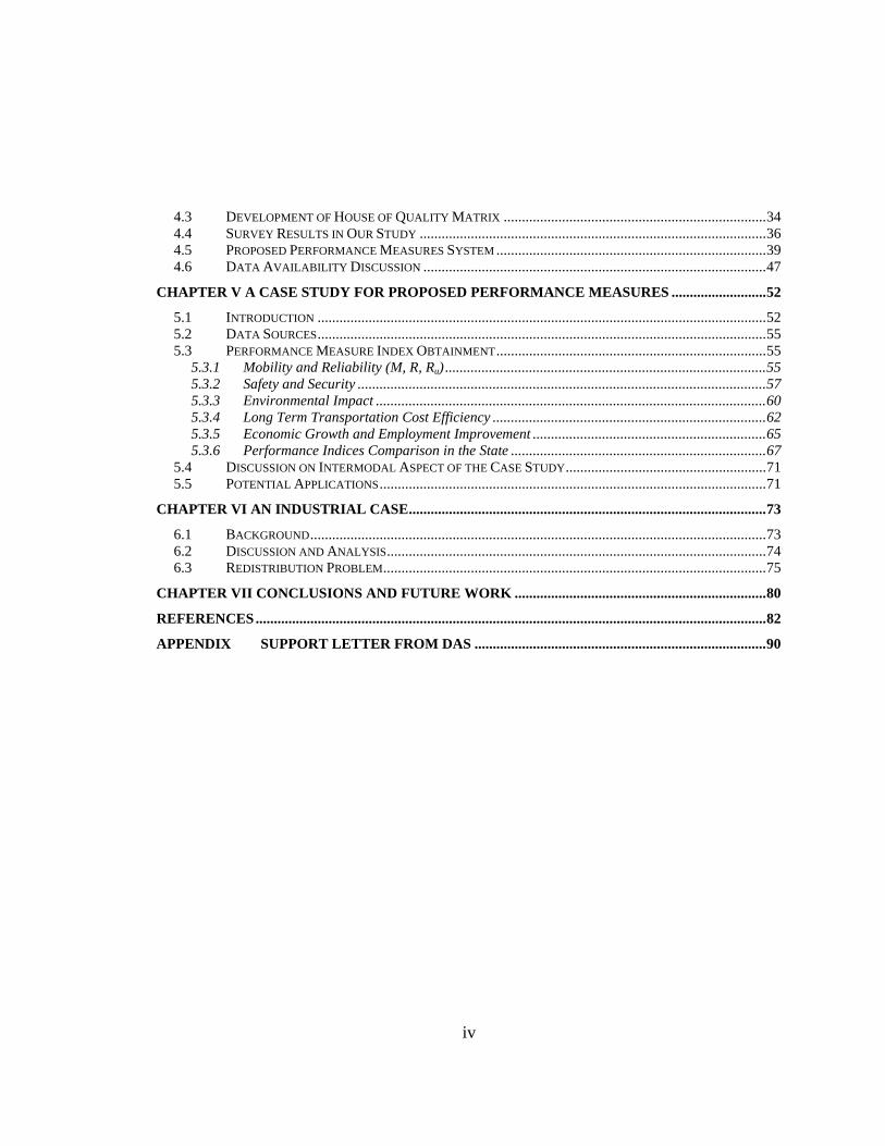
4.3 DEVELOPMENT OF HOUSE OF QUALITY MATRIX ........................................................................34 4.4 SURVEY RESULTS IN OUR STUDY ...............................................................................................36 4.5 PROPOSED PERFORMANCE MEASURES SYSTEM ..........................................................................39 4.6 DATA AVAILABILITY DISCUSSION ..............................................................................................47

CHAPTER V A CASE STUDY FOR PROPOSED PERFORMANCE MEASURES ..........................52 5.1 INTRODUCTION ...........................................................................................................................52 5.2 DATA SOURCES...........................................................................................................................55 5.3 PERFORMANCE MEASURE INDEX OBTAINMENT..........................................................................55

5.3.1 Mobility and Reliability (M, R, Ru)........................................................................................55 5.3.2 Safety and Security ................................................................................................................57 5.3.3 Environmental Impact ...........................................................................................................60 5.3.4 Long Term Transportation Cost Efficiency ...........................................................................62 5.3.5 Economic Growth and Employment Improvement ................................................................65 5.3.6 Performance Indices Comparison in the State ......................................................................67

5.4 DISCUSSION ON INTERMODAL ASPECT OF THE CASE STUDY.......................................................71 5.5 POTENTIAL APPLICATIONS..........................................................................................................71

CHAPTER VI AN INDUSTRIAL CASE..................................................................................................73 6.1 BACKGROUND.............................................................................................................................73 6.2 DISCUSSION AND ANALYSIS........................................................................................................74 6.3 REDISTRIBUTION PROBLEM.........................................................................................................75

CHAPTER VII CONCLUSIONS AND FUTURE WORK .....................................................................80 REFERENCES............................................................................................................................................82 APPENDIX SUPPORT LETTER FROM DAS ................................................................................90

v

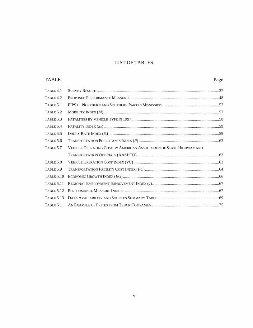
LIST OF TABLES TABLE Page TABLE 4.1 SURVEY RESULTS ....................................................................................................................37 TABLE 4.2 PROPOSED PERFORMANCE MEASURES.....................................................................................48 TABLE 5.1 FIPS OF NORTHERN AND SOUTHERN PART IN MISSISSIPPI ......................................................52 TABLE 5.2 MOBILITY INDEX (M) ..............................................................................................................57 TABLE 5.3 FATALITIES BY VEHICLE TYPE IN 1997....................................................................................58 TABLE 5.4 FATALITY INDEX (SF) ..............................................................................................................59 TABLE 5.5 INJURY RATE INDEX (SI) ..........................................................................................................59 TABLE 5.6 TRANSPORTATION POLLUTANTS INDEX (P) .............................................................................62 TABLE 5.7 VEHICLE OPERATING COST BY AMERICAN ASSOCIATION OF STATE HIGHWAY AND

TRANSPORTATION OFFICIALS (AASHTO)...............................................................................63 TABLE 5.8 VEHICLE OPERATION COST INDEX (VC) ..................................................................................63 TABLE 5.9 TRANSPORTATION FACILITY COST INDEX (FC) .......................................................................64 TABLE 5.10 ECONOMIC GROWTH INDEX (EG) ............................................................................................66 TABLE 5.11 REGIONAL EMPLOYMENT IMPROVEMENT INDEX (J) ................................................................67 TABLE 5.12 PERFORMANCE MEASURE INDICES ..........................................................................................67 TABLE 5.13 DATA AVAILABILITY AND SOURCES SUMMARY TABLE...........................................................69 TABLE 6.1 AN EXAMPLE OF PRICES FROM TRUCK COMPANIES.................................................................75

vi

LIST OF FIGURES FIGURE Page FIGURE 4.1 GEOGRAPHIC DISTANCE BETWEEN ORIGIN AND DESTINATION................................................39 FIGURE 4.2 FATALITIES FOR DIFFERENT MODES IN URBAN AND RURAL AREAS........................................43 FIGURE 4.3 MONEY FLOW DIAGRAM FOR A TRANSPORTATION SYSTEM....................................................45 FIGURE 5.1 COUNTIES IN THE STATE OF MISSISSIPPI ..................................................................................53 FIGURE 5.2 NORTHERN PART OF MISSISSIPPI AND SOUTHERN PART OF MISSISSIPPI ..................................53 FIGURE 5.3 HIGHWAY TRANSPORTATION NETWORK IN THE STATE OF MISSISSIPPI ...................................54 FIGURE 5.4 NETWORK GRAPHIC COMPARISONS IN THE NORTHERN AND SOUTHERN MISSISSIPPI ..............54 FIGURE 5.5 TRAFFIC ASSIGNMENT RESULTS-1...........................................................................................56 FIGURE 5.6 TRAFFIC ASSIGNMENT RESULTS-2...........................................................................................56 FIGURE 5.7 SCREENSHOT OF FATALITIES IN MISSISSIPPI IN 1997 BY COUNTY ............................................58 FIGURE 5.8 SCREENSHOT OF FARS DATABASE ON INJURY QUERY............................................................60 FIGURE 5.9 SCREENSHOT OF EMISSION SUMMARY REPORT IN MISSISSIPPI IN 1996 ...................................61 FIGURE 5.10 AVERAGE PERSONAL INCOME BY COUNTY IN THE STATE OF MISSISSIPPI ...............................65 FIGURE 5.11 AVERAGE WAGES PER JOB IN THE STATE OF MISSISSIPPI ........................................................66 FIGURE 6.1 MAPS OF THE DEALERS DIRECTLY SERVED BY TRUCKS FROM CANTON..................................73 FIGURE 6.2 RAIL DISTRIBUTION FOR NORTHWEST REGION FROM THE FOUR ORIGINS ...............................74 FIGURE 6.3 REDISTRIBUTION ILLUSTRATION..............................................................................................77

vii

LIST OF NOTATIONS AND UNITS

AN – Set of total trips for a typical year. ATC – Annual equivalent total cost (dollars). EG – Economic growth index. It denotes total economic growth per dollar of investment (percent per dollar). FC – Facility cost per operation cost TMR or PMR (dollars per ton mile required or dollars per passenger mile required). Fi,j,n – Fatality for a specific trip n between each OD. fi,j,n – Expected travel time for a specific trip n between OD pair i and j(hours). GCp – Fuel consumption cost involved in trip (i,j,n) (dollars). Ii,j,n – Number of injuries for a specific trip n between each OD. J – Job improvement index. It denotes number of job years created by transportation per dollar of investment. L – Community livability index. It denotes the percent of people affected by transportation system. L* – Traffic Load (no unit). li,j – Geographic distance between OD (miles). M – Mobility (hours per mile). N – The set of all trips. P – Pollutants index. It denotes tons of mobile source emissions per TMR or PMR (tons per ton mile required or tons per passenger mile required). POi,j,n – Tons of mobile pollutants involved in trip (i,j,n) (tons).

viii

pi,j,n – Number of tons or passengers involved in trip i,j,n, where i is the origin (O), j is the destination (D), and n is the index of the trip with the same OD. R – Reliability (no unit). Ru – Reliability due to unexpected travel delay (no unit). SF – Fatality rate. It denotes the number of fatalities per TMR or PMR. SI – Injury rate. It denotes the number of injuries per TMR or PMR. Sp – Property damage cost caused by accidents in trip (i,j,n) (dollars). TEG – Total economic growth. TI – Total investment (dollars). TJ – Total created job years due to the transportation system. TMR or PMR – Ton-miles Required or Passenger-miles Required, which is the multiplication of pi,j,n and li,j (ton-miles required or passenger-miles required). Ti,j,n – Total travel time between each OD for a specific trip n (hours). Tk – The traveling time on link k for the nth trip between each OD (hours).

CV – Volume over Capacity ratio (no unit).

VAi,j,n – Vehicle aging cost involved in trip (i,j,n) (dollars). VC – Vehicle operation cost per TMR or PMR (dollars per ton mile required or dollars per passenger mile required). VIi,j,n – Vehicle insurance cost involved in trip (i,j,n) (dollars). VMi,j,n – Vehicle maintenance cost involved in trip (i,j,n) (dollars). VOi,j,n – Other vehicle operation cost involved in trip (i,j,n) (dollars).

1

CHAPTER I INTRODUCTION With an increased emphasis on intermodal transportation, the issue of how to

evaluate an intermodal transportation system is getting more attention since the enactment of the Intermodal Transportation Efficiency Act (ISTEA) [1] and the Transportation Equity Act for the 21st Century (TEA-21) [2]. In this chapter, the research background, purpose and scope, and anticipated research results for this study are discussed. The background study is mainly focused on the U.S. DOT practices, federal laws on intermodal transportation systems, and states & agencies’ practices in intermodal transportation system performance measures.

1.1 Background According to the United States Department of Transportation’s (U.S. DOT)

Strategic Plan [3], two major goals of U.S. transportation development are to “support a transportation system that sustains America’s economic growth” and to “shape an accessible, affordable, reliable transportation system for all people, goods, and regions”. In response to the U.S. DOT’s strategic plan, the Federal Highway Administration (FHWA) has also enacted its own strategic plan and put productivity and mobility as their major considerations. The major goals in the FHWA strategic plan are to “continuously improve the economic efficiency of the Nation's transportation system to enhance America’s position in the global economy” and to “continually improve the public's access to activities, goods and services through preservation, improvement and expansion of the highway transportation system and the enhancement of its operations, efficiency and intermodal connections” [1]. In order to reach these goals, transportation practitioners and researchers have been trying to improve the efficiency of intermodal transportation for decades. In 1991, ISTEA was enacted, and its passage established the important role of intermodal transportation in United States transportation [1]. The objective of ISTEA is “to move goods and people in an energy efficient manner, provide the foundation for improved productivity growth, strengthen the nation’s ability to compete in the global economy and obtain the optimum yield from the nation’s transportation resources [1].” In 1998, the TEA-21 was enacted, which was the second landmark for intermodal transportation system development [2]. It provides the state Department of Transportations (DOTs) more investments and opportunities to develop the national intermodal transportation system.

In response to all these strategic goals and federal laws, the Office of Operations in FHWA, a leading transportation development agency in the U.S., considers improving transportation efficiency as their kernel task. In particular, one important goal of their work plan is to “develop freight metrics, collects data, and analyzes goods movement trends” by Freight Policy Team in the Office of Operations [5].

2

A well developed performance measure system is critical to the success of developing an efficient intermodal transportation system. In 1993, the Government Performance and Results Act (GPRA) established a requirement for federal agencies to identify goals and measurable outcomes to gauge performance to meet program objectives [6]. The objective of GPRA is to shift the focus of government decision-making, management, and accountability from activities and processes to the results and outcomes achieved by federal programs. Under GPRA, annual performance goals and performance outcomes should be reported to the congress by each federal agency. In the report submitted by the U.S. DOT to the U.S. Congress on the status of the nation’s surface transportation system in June 2001 [6], some planned outcome and performance measures have been presented. ISTEA also requires that all states implement a performance based planning process [4]. Since then, many states and MPOs conduct studies related to performance measures of intermodal transportation. The states of Minnesota, Oregon, Florida, California, along with the San Francisco Bay Area are on the front line of enacting their own performance measures.

Although there are numerous performance measures in literature, there is no scientific and systematic measure system that can be used to evaluate intermodal transportation alternatives because of various problems. Most MPOs and state DOTs claimed in a survey that they just don’t know how to design or plan an intermodal transportation system and cannot find enough related methodologies, though they have already realized its importance [7]. Many existing performance measures can be applied only for a single mode since different administrations, which are organized based on modes in the U.S. DOT, developed these performance measures separately. For instance, the safety in airborne transportation is usually measured by the accident rate per take-off, no matter how many passengers are involved. The figure cannot be directly used to compare the accident rate in highway system, which is usually defined by the number of casualties per one million passenger mileages. The lack of uniform measures, which can be used for all modes, makes it hard to compare alternatives and make a mode choice decision. Rutherford [8] pointed out mobility, which is defined as highway level of service cannot lead to multimodal solutions. The scarcity of a well-organized system is another common problem of transportation measures. For example, for freight transportation, the goal of accessibility of intermodal facilities (internal and external measures) and the goal of connectivity between modes (ease of intermodal connection) are two usual measures along with mobility (which is measured by the average traveling time per trip). However, connectivity and accessibility are really factors influencing mobility so that they are measures for some parts of the system rather than the whole system. The overlap can also be widely observed in other categories or classifications of the performance measures. Most current measures are developed from engineering design viewpoints rather than based on the needs of the transportation users. A study on a

3

systematic and user oriented performance measure system is necessary to address all of the above problems.

1.2 Purpose and Scope The objective of this study is to develop a systematic and user oriented

performance measure system for intermodal transportation systems. The performance measure system will be tested in a case study in the State of Mississippi. This study also includes an analysis for a major automaker to investigate their mode choice decisions. In the future, these performance measures can be integrated into other models such as Virtual Intermodal Transportation System (VITS) to answer several key intermodal transportation performance measures related questions:

• For a transportation system, intermodal or single mode, how well it is designed and operated;

• For a specific industry in a specific area, what kinds of modes or their combination should be chosen;

• For local, statewide, or national governments, what kind of intermodal transportation system is the best choice (here one single mode can be the choice).

A good performance measure system for an intermodal transportation system is not a simple combination of those defined on each single mode, but should be carefully defined from the system viewpoint. For instance, to measure mobility for intermodal transportation, we need to consider not only the traveling time on each mode but also the transfer time between two consecutive modes, which depends on coordination among the modes. How to quantify all qualitative measures and demonstrate its usability are the main tasks in this research.

System engineering principles and techniques will be applied in this research. System engineering is an interdisciplinary approach encompassing the entire technical effort to evolve and verify an integrated and life cycle balanced set of systems, people, product, and process solution that satisfies customer needs [10]. Top-down method analysis will be used with other techniques like requirement analysis, quality house method, and trade-off analysis.

1.3 Anticipated Study Results Systematic performance measures will be major aspects of this study. The study

will yield a number of valuable results including: • Complete and detail review of transportation performance measures practice

• Standardized transportation development goals

• Need identification of transportation users

4

• Methods for transportation performance measure modeling

• Proposed performance measure system

• A case-based performance measure study

• Performance measure system applications in industry

The resulting systematic performance measure system can facilitate the process of evaluating intermodal transportation systems and choosing transportation modes. The benefit of intermodal transportation can be systematically depicted so that it can improve the education on intermodal transportation and help more people to consider intermodal transportation during transportation planning and transportation design.

5

CHAPTER II OVERVIEW OF PERFORMANCE MEASURES IN LITERATURE

A good performance measure system is critical to the success of an intermodal transportation system design and the required performance should be identified at the very beginning of system design. Therefore, many national, local, and academic studies have been putting tremendous effort on intermodal transportation performance measures research in recent years. This chapter is to review, summarize, and evaluate those practices and studies. The review is mainly based on research results of states and MPO practices, and the measures are categorized into groups with a detailed discussion and analysis. General goals for a transportation system are given first in this chapter as a basis for the detailed analysis.

2.1 General Goals of a Transportation System Performance measures for different modes of transportation have been studied by

committees of the Transportation Research Board (TRB) and other agencies for more than a decade. The very first step in determining the performance measure of a transportation system is to identify goals and objectives for different modes and for the system. The selection of goals and objectives should directly reflect the customer needs and the economic costs associated with it. The basic goals for transportation can be summarized by the following factors:

Mobility: Ease of movement of people, goods, and services.

Accessibility: Ease of reaching transportation facilities. Accessibility is also relates to use of transportation facilities by disabled persons and relates to whether or not people can get to transportation facilities.

Safety: Risk of accident or injury as measured by crashes.

Environmental: Preservation of the existing state of the environment.

Public Involvement: The degree to which populations participate in transportation decision-making.

Mobility strategic goal is to ensure a transportation system that is accessible, integrated, fast, efficient, and flexible. According to a study made by the U.S. DOT on goals for different modes [11], the main goal of a highway system is to reduce transportation time from origin to destination for individual transportation users to achieve mobility. The effort to meet the goal includes increasing miles of the highway system, reduction of the number of deficient bridges on the highway system,

6

implementation of intelligent transportation system (ITS), and delay reduction on federal-aid for the highway system. Similarly, for an airborne transportation system, the strategic goals for mobility include, making aviation speedier, using higher technologies to fly in bad weather, providing the quickest path for the flight, and making more runways. Safety is another important goal in transportation systems. A transportation system without any safety measures cannot be considered a perfect system. Safety measures are differentiated according to different modes in current practices. For example, the goals for a highway system are described as the reduction in highway fatalities per 100 million vehicle-miles traveled and reduction in large truck related fatalities per 100 million truck vehicle-miles traveled by a study conducted by the U.S. DOT [12]. For airborne systems, the goals described are to reduce the commercial aviation fatal accident rate per 100,000 departures and to reduce general aviation accidents. The safety goal of railways is to reduce rail accidents and incidents per million train-miles. Transit goal is described as a reduction in the transit fatality rate. Furthermore, according to the U.S. DOT performance plan, the safety goals required for the whole transportation system are described as a reduction in highway related injuries, reduction in highway fatalities due to alcohol, and an increase in the usage of safety belts [13].

Another concern related to a transportation system is the effect of the transportation system on the environment. Intensive research is currently being conducted worldwide in this area. According to a study by the U.S. DOT [14], the main strategic goals for human and environment factors are to improve the sustainability and livability of communities, reduce the adverse effect of transportation or ecosystems and the natural environment, improve the viability of ecosystems, and most importantly, reduce the amount of pollution from transportation sources. Besides these, the goals of a transportation system should also be concerned with the reduction of the noise level, reduction in deforestation, and the efficient use of land.

2.2 Classifications of Transportation Performance Measures In general, performance measures can be classified as either qualitative or

quantitative. Quantitative performance measures can be valued with a number such as average time of a travel, cost per ton-mile, and so on. Qualitative performance measures are those hard to be quantified and are indicative measures for system efficiency. Although some of the performance measures are hard to quantify directly, a generalized model, which quantifies and combines all performance measures, can give a simple guidance for decision-making.

Based on different levels, performance measures can be classified into three groups: infrastructure performance measures, operational performance measures, and user level performance measures. Infrastructure performance measures in transportation involve connections to transportation systems, intermodal facilities, and principle markets; operational level performance measures can be used to evaluate environmental

7

impacts and service level; total travel time, delays, costs, freedom of scheduling, mode choice flexibility, and route choice flexibility are some user level performance measures. All these three levels of performance measures interact with each other. For instance, the infrastructure performance measures can influence the user level performance measures because connection between different modes and accessibility of intermodal facilities can affect the total travel time.

Using transportation industry productivity or transportation highway performance measures proposed by Hagler Bailly Services, Inc. is another classification [15]. Some measures are concerned with transportation industry productivity, while others are direct indicators of transportation system efficiency. The former addresses the service efficiency that the industries can provide rather than that of a transportation system. Indicators of labor productivity, logistics efficiency, and equipment utilization fall into this classification. These measures do not directly indicate transportation performance. For example, the percentage of empty trucks in a system is not a direct reflection of the efficiency of the transportation system since it decided by industry needs and practices. The latter set can be directly used to evaluate the efficiency of a transportation system such as the accident rate.

There are eight categories of performance measures of a transportation system in some other literature: [15,16] mobility and accessibility performance measures; reliability measures; safety measures; environmental measures; cost measures; infrastructure condition measures; economic impact measures; and industry productivity.

2.3 General Problems of Performance Measures in Literature After an intensive literature review, many problems have been found in the

existing performance measure system for a transportation system. These problems include failure to distinguish measure and factors, not user-orientated measures, unsystematic models, and scarcity of quantitative models.

Measures usually refer to those that can directly reflect the performance of a transportation system. In current literature, many indirect indicators are classified into a performance measure system. For example, the delay caused by an accident will affect the average travel time and reliability of the transportation network. However, it fails to be a direct indicator of the efficiency of the transportation system. Rather than being listed along with the average travel time, the delay should be classified into the second tier performance measures, indirect performance measures, or factors affecting performance measures to avoid the overlap. These aspects of the practice on transportation performance measures need to be further investigated in future studies.

A transportation system is designed, constructed, and operated to meet people’s needs. All performance measures should be about user satisfaction. Different users may require different ranges of transportation service quality. To define the performance measures accurately, user classification and user needs should be identified first. For

8

example, the government agencies are expecting better transportation system with higher traffic volume, but private industries are expecting quicker and safer service. Sometimes, we have to make a tradeoff in the analysis since contradicting interests may exist.

A transportation system is a tremendously complicated system with millions of people and numerous factors involved, so system engineering principles should be adopted. Many performance measures have been intuitively proposed instead of through a top-down systematic method. They are, therefore, likely to neglect some points and fail to get a complete and reasonable picture of the system. Failure to distinguish measure and factors is one outcome of not using system perspective analysis. Many performance measures are appropriate for only some segments of transportation, like one single mode, and cannot be used to evaluate the whole intermodal system.

2.4 Discussion and Evaluation of Performance Measures in Literature In this section, major performance measures in the literature are reviewed,

discussed, and evaluated in detail by categories. The review shows that a standardized tranportation performance measure system is needed.

2.4.1 Mobility and Accessibility

Since the main purpose of transportation is to move goods and people from origins to destinations, mobility is one important indicator on how well a transportation system functions. In general, mobility can be defined as the ability to transport goods, and people efficiently. The average travel time is widely used to measure the efficiency. For example, average origin-destination travel time per trip is introduced by Meyer [17].

Speed (mile/hr) and travel length (mile/trip) are two main determinants for the total travel time of a specific trip. Most researchers like Bertini and Shaw [18,19] consider average speed as the main factor to decide mobility, while researchers in Albany studies consider both speed and trip length mobility measures [20]. Speed is heavily dependent on the congestion conditions. On highways, congestion is usually measured by total highway segment lengths with a Volume to Capacity ration (V/C) greater than 0.85 [16,18]. The Colorado performance measure system approximately gets the total travel time per trip by dividing the total traveling distance by the average speed [16]. They define Passenger Mobility Coefficient by using PMT/Average Speed/1,000,000, where PMT means passenger miles traveled for the passenger transportation and Freight Mobility Coefficient by using FTMT/Average Speed/1,000,000, where FTMT means freight ton miles traveled. Different transportation systems or modes have different capacities and the above coefficients cannot simply be used to compare the systems with different capacities because the larger the system, the larger the values of the above

9

coefficients will be due to the larger PMT or Vehicle Miles Traveled (VMT). For example, California definitely has a larger coefficient than Delaware, but it is hard to say whether California has a better system than Delaware based only on this coefficient. Therefore, some uniformalized indexes are necessary to compare the systems with different capacities. BRW and Bertini [16,18] use the Passenger Mobility Index and Freight Mobility Index for the mobility of passenger transportation and freight transportation, respectively. Passenger Mobility Index is (PMT/VMT) × Average Speed, where PMT means passenger miles traveled, VMT denotes vehicle miles traveled, and their division is the loading efficiency for each vehicle. Similarly, Freight Mobility Index is FTMT/Truck VMT*Average Speed, where truck VMT denotes truck vehicle miles traveled. Mobility index can be used to reduce complexity and volume of performance measures and compare the performance of different facilities among different modes. However, the index may be in favor of public transportation systems because of their larger loading efficiency, and it may, therefore, yields wrong conclusions. For example, if there are only two passengers for a trip, a big bus would not be better than two personal cars, while the mobility index conforms with the former. In general, estimating the total traveling time (or index) by the product of total travel distance (or loading efficiency) and the average speed is an approximation and could be inaccurate. In some cases, not only the average speed but also the variance of speed can have significant impact on the total traveling time.

In general, total traveling time or its approximation by division of trip length by average speed are commonly used in literature to evaluate mobility. Though some people also consider the capacity effect on the measures, capacity can still not represent the mobility needs of the passengers and freight and may make inappropriate comparisons among different systems.

The total time from origin to destination is not a simple sum of the traveling time on each mode. The time from the origin and destination to the transportation system and the transfer time between two consecutive modes in an intermodal transportation system also significantly contribute to the total traveling time. Bertini et. al.[18] use number (or percent) of intermodal connectors improved by operational strategies to evaluate the efficiency. They also use percentage of intermodal connectors which have been improved due to the strategies applied and time to access intermodal facilities to evaluate the accessibility of the intermodal facilities [18]. Since this group of performance measures include major factors affecting the average travel time, it will be more appropriate to define this set of performance measures as the factors or second tier measures affecting the average travel time instead of first tier performance measures, which are parallel to the average travel time, as the measure for mobility.

Accessibility is another major concern in the literature for transportation systems. The number of goods transfered and number of people accessing the system are considered to be indicators of transportation accessibility by Bertini and El-Geneidy [21].

10

This set of performance measures has the same representation as the performance measure like ease of movement and ease of access, which may be difficult to measure quantitatively. Connectivity is a major factor affecting the overall travel time and the accessibility of a transportation system. Percentage of urban population within X mile of transit is used by [21,22,23] to evaluate the transit service accessibility. Percentage of employment sites within X miles of major highways is another similar factor used by [23] to evaluate the accessibility or connectivity of the system. Percentage of population within X minutes of Y percentage of employment sites considers the overall impact of the two measures mentioned above. However, this set of performance measures are some major factors affecting the average total traveling time, and we believe they should be second tier measures rather than system measures. At the same time, other accessibility related issues can not be ignored. For example, the accessiblibility of transportation facilities to disabled people or whether the facilities are reachable. These considerations on accessibility will mostly be related to transportation terminal analysis. For subsystem performance measures, this might be a very important consideration.

The capacity of transportation system is considered to be a very important performance measure in much of the literature. Different papers use different names for capacity, which essentially all have the same meaning. BRW Inc. and Bertini [16,18] use Vehicle Miles Traveled (VMT), Person Miles Traveled (PMT), and the division of PMT/VMT to represent the capacity of the system. For freight transportation analysis, truck vehicle miles traveled, truck freight ton-miles traveled, and truck freight ton-miles traveled/truck vehicle miles traveled can be used to represent the system capacity [16]. Vehicle hours traveled and passenger hours traveled are used by Bertini and Shaw [18,19] for passenger transportation systems. Passenger hours traveled can be calculated by using VMT and the Average Vehicle Occupancy (AVO) i.e., the total volume of people using the system. In this set of performance measures, occupancy and less than truck load (LTL) are given much attention. Truck freight ton-miles traveled (TMT) is used by the Colorado Department of Transportation to represent the capacity of the transportation system [16]. In fact, the above are throughput rather than capacity. Although not linearly, mobility decreases with capacity increase for a given demand. Therefore, capacity is a factor influencing mobility rather than a separate system level measure.

2.4.2 Reliability

For a transportation system, the reliability is usually represented by the delay caused by some unusual events or incident such as accident delay, intersection delay, intermodal terminal delay, or other lost time. Level of congestion is used by BRW Inc. to denote one aspect of the reliability of transportation systems [16]. Delays are measured by different researchers in quite a different fashion, for example, transferring time

11

between modes [15, 21, 24], delays per ton-mile, lost time or delay time, and congested highway miles divided by total highway miles [16]. These sets of performance measures generally have the same theme in terms of the reliability of a transportation system. Travel time reliability was proposed by the Washington State Department of Transportation to determine the best available tools and methods for collecting travel time data on a real time basis and recommending a methodology to determine travel time reliability [25]. The main problem of the above measures is how to define delays which are based on people’s expectation.

On-time performance is commonly considered to be a major indication of transportation efficiency especially for the evaluation of a transit system [26]. Frequency of transit service is used by the State of Florida to evaluate a transit system [26]. However, on-time performance fails to consider the fact that on time doesn’t mean that the system is performing better. For example, if one company promised to deliver your needed parts within 100 days and the company really successfully delivered the needed parts on time with deliveries frequently occurring in 10 days or 90 days does not necessarily mean that this company has good performance.

2.4.3 Safety and Security

Safety is an inherent performance measure for transportation. A transportation system without high safety is unreliable and inefficient. For example, a highway system may have accidents due to the lack of carefulness such as driving under the effect of alcohol. An airborne transportation system safety is threatened by lack of information and technical failures. Inexperience recreational boaters can reduce the safety of maritime transportation, while the communication condition at cross sections is critical to keep high safety for rail transportation.

According to a performance report by the U.S. DOT [27], the most common indicators with respect to safety are fatalities per 100 million vehicle-mile of travel and number of accidents per 100 million vehicle-miles of travel [27]. As we have described above, different modes have different causes to influence safety, so safety measures are different according to the mode for different modes in the literature. For example, for highways, the measure is usually the number of fatalities within a certain length of vehicle miles travel; while for airborne transportation, the measure is usually identified by fatal aviation accidents per 100,000 departures [27]. Furthermore, this measure can be used to calculate the average number of fatalities per 100,000 passenger miles by considering AVO (Average Vehicle Occupancy). Similarly, maritime safety can be determined by the number of recreational boating fatalities per year. Another important indicator of safety measure given by the U.S. DOT for maritime safety measures [27] is the number of calls received for help by the coast guard and the percent of all mariners in imminent danger who are rescued. A decrease in the number of calls received by the

12

coast guard and a decrease in the percentage of mariners in imminent danger will represent an improvement in performance of maritime safety. Due to a common lack of unawareness among recreational boaters, maritime safety is mostly concerned with the safety of recreational boaters and, hence, their main goal is to reduce fatalities associated with this and to increase awareness. For railways, 50 percent of the rail related fatalities are trespasser-related, and more than 45 percent occurred at highway-rail grade crossings [27]. The most important performance measures associated are train accidents per million train-miles and rail related fatalities per million train-miles. These performance measures will give the number of accidents and corresponding fatalities within a certain distance of railway-miles. Once again, we can use AVO to calculate the number of fatalities corresponding to the number of accidents per million train-miles. According to the study [27], the transit system is also considered as one of the major modes of a transportation system and is considered one of the safest modes. It is measured by indicators like transit fatalities per 100 million passenger-miles traveled or transit-injured persons per 100 million passenger miles traveled.

The measures mentioned above are the main performance measures indicating safety in the literature. Besides these, transportation is also associated with many other safety measures: for example, average time between notification and response/arrival clearance, total duration of incidents, etc. These measures represent the speed of response for any accident. Since a delay caused by an accident could heavily affect the economic value corresponding with it and, as a result, the customer satisfaction will be harmed by the sluggish service by the system, a transportation system needs to be very responsive.

In general, accident rates, fatality rates, and injury rates are directly related to the loss due to accidents. The figures of these rates directly reflect the safety performance of a transportation system. Amount of damaged property and level of maintenance in a year is correlated to the cost incurred by transportation activities instead of to an independent measure of the performance of a transportation system. Accident rates at major intermodal terminals are a subset of the total accident rates, and they should not be a direct reflection of the whole transportation system performance. The performance measured by the number of high accident locations can be reflected in the accident rate measure as well. The number of vehicles transferring dangerous goods in a particular region is also not an appropriate safety performance measure to evaluate a transportation system, since this number is usually required by the needs of industries or government agents, and transportation system design cannot change the value.

The number of accidents, fatalities, and injuries are some appropriated performance measures to evaluate the safety of a transportation system. How to scientifically define them so that they can be used for all modes is a key issue. As we can see, researches have different definitions on this set of performance measures, and they are usually mode specific. Some definitions are based on time, while others are based on vehicle trips.

13

Traffic security and crime rates are also one type of transportation system performance. This set of performance measures can also be defined based on the ton-miles traveled or passenger miles traveled.

Public security and homeland security is another big concern of transportation. Many of the highway systems are intentionally built to improve homeland security by facilitating the logistics in an emergency. As this topic becomes more important after September 11, 2001, this set of performance measures should also be considered in the safety and security category.

2.4.4 Environmental Performance Measures

One major tradeoff associated with a transportation system is its impact on both the human and natural environment. We enjoy the service from transportation, but at the expense of the environment. In the long run, the sustainability of a transportation system is affected by its impact on the environment [28]. The DOT has identified four strategic goals for the environment which include: reduction of transportation related pollutants and green house gas release, construction, and operation of transportation facilities, improvement of the sustainability and livability of the communities, and improvement on the natural environment and communities affected by DOT-owned facilities and equipment.

Estimating the emissions from all the mobile sources is a major step in setting up the performance measure for the system. The DOT uses “Tons (in millions) of mobile source emissions from one-road vehicles” as one of the major performance measures [28]. Some studies also define performance measure based on the type of emissions from the transportation sources. For example, the DOT has given metric tons (in millions) of carbon equivalent emissions or green house gas emissions from transportation sources. The Environment Protection Agency (EPA) also determines the impact on the environment based on a criterion of pollutants [29]. In 1999, on-road transportation sources accounted for 51% of carbon monoxide (CO), 34% of nitrogen oxides (Nox), 29% of volatile organic compounds (VOC), and 1% per particulate matter (PM). Based on these estimated tonnages of on-road mobile sources i.e., CO, Nox, VOC, and PM, FHWA developed an annual emissions level. Based on this annual emission and the total vehicle miles traveled in a year, the total emission per vehicle miles can be calculated easily. Besides on-road vehicles, there is also a significant amount of pollution in waterborne and pipeline transportation systems. Thousands of gallons are being spilled in oceans every year, polluting the water. A common performance measure for all modes could be the amount of gallons spilled per ton-miles. All modes fragment or destroy habitat, which can be measured in terms of area affected.

Noise is another unwanted effect of transportation. Aviation and railways are main contributors of noise pollution. In recent years, noise complaints have increased

14

drastically, and reducing noise has become one of the most aspired needs of communities. A study by the U.S. DOT uses the number of people who are exposed to significant noise levels [14] as the measure for the noise effect of transportation. The level of noise is usually determined by decibel (db), so the number of people being affected by a significant decibel of noise or percent of people affected by transportation noise can be a good performance measure.

2.4.5 Cost Measures

The costs discussed here just include the direct costs associated with transportation planning, construction, and operation. Other costs, like those caused by accidents, delay, and pollutants, are considered in other performance measures.

The cost of highway freight per ton-mile identified by Hagler Bailly Services, Inc, Hickling Lewis Brod, Inc, and the State of Florida [15,30,31] is related to freight operation cost. Fuel consumption cost is a major factor affecting the total operating cost, so it can be categorized into second-tier performance measure for operating cost. Truck technology and drivers’ wages can also be second-tier performance measures or factors affecting total operating cost rather than some system level performance measures as identified by Hagler Bailly Services, Inc. and the Florida DOT [15,31]. Cost per vehicle hour was used by [15] to represent long term cost efficiency for a transportation system, which is pretty similar to that proposed by Hagler Bailly Services, Inc. [15]. However, using vehicle hour as the base loses the flexibility of considering the Less Than Truck Load (LTL) vehicles for freight transportation or vehicle occupancy for passenger transportation.

The maintenance cost of facilities is another direct cost, and many state DOTs [15, 31] actively fund research for maintenance related studies. However, higher (or lower) maintenance costs do not mean a better transportation system, and more spending on highway maintenance does not necessarily indicate an improvement in road conditions. In this sense, it is not a systematic transportation performance measure but just a description of a fact. Of course, maintenance cost is a part of transportation operation cost.

2.4.6 Infrastructure Condition Measures

This set of performance measures is used to indicate the infrastructure conditions of transportation systems. Whether the infrastructure is in good condition or not will directly affect average travel time or the reliability of transportation systems.

The number of bridges per 100 miles and the number of deficient bridges per 100 miles are used by BRW Inc. to measure highway infrastructure condition [16]. Although sometimes the travel time may be reduced because of more deficient bridges, it is not an

15

appropriate set of measure for evaluating the infrastructure condition because of no consideration on the geological condition.

Performance measure of lane-miles of high-level highway requiring rehabilitation is used by “1998 California Transportation Plan: Statewide goods movement strategy” to denote the infrastructure condition [32]. This measure could be a direct reflection of infrastructure condition. However, it fails to be a performance measure for transportation system efficiency.

Performance measure presented by the Michigan Department of Transportation on infrastructure conditions are as follows: the percentage of miles of state trunk lines with surface condition classified as good and the number bridges rated as good [33]. Similar concepts may be applied for all modes of transportation systems. For example, the percentage and total length of different levels of classifications of highways or different grades of railroad infrastructure can be a good performance measure for evaluating transportation infrastructure [33]. In general, infrastructure performance measures discussed in the literature are generally not direct performance measures for transportation system evaluation but rather are some factors affecting travel time or maintenance cost, etc. If they are listed along with mobility and reliability measures, there are some big overlaps. We suggest they be second tier measures or factors.

2.4.7 Economic Impact Measures

Economic impact measures identified in previous studies are generally used to evaluate the economic benefits generated from transportation systems or transportation activities. The benefit, together with the total life-cycle cost, is the basis for cost-benefit analysis that will be a direct reflection of the performance of transportation systems.

The number of direct and indirect jobs created is considered to be one type of economic impact measure [34, 35]. If more jobs are created during transportation construction and operation, the transportation system is more effective in terms of solving employment problems. However, more jobs created do not mean more benefits. The unit benefit of jobs created should also be considered in this case.

The contribution of investment to GDP growth presented by Hickling Lewis Brod, Inc. denotes the GDP growth [30]. This could be a very effective performance indicator of a transportation system. The State of Florida uses revenue per ton-mile by mode as a performance measure for economic development [31]. This benefit is an indirect monetary benefit of a transportation system and related to mobility. When a system is under evaluation, the overlap between economic development and mobility benefits should be avoided.

The value of the freight that is moved from, to, and within the region to develop an overall (direct, indirect, and induced) economic impact is used by the St. Louis Region MPO [35] as economic performance measures. The value of the freight the transportation

16

system carries has little relationship with the performance of the transportation system. It is not an appropriate performance measure for evaluation of transportation system efficiency.

In general, economic impact measure is a set of measures that is hard to measure since they will be closely related to the economic condition improvement in the region. Usually, it is difficult to determine how many of them result from a transportation system.

2.4.8 Industry productivity

The literature shows that industry productivity is a set of performance measures for the efficiency of the industry instead of the transportation system. They are independent with the performance measures related to transportation systems. Thompson [36] uses vehicle miles per capita, passenger trips per capita, revenue hours per employee, and passenger trips per employee to evaluate industry productivity.

In a report examining of transportation industry productivity measures distributed by FHWA and the U.S. DOT [37], performance measures of empty/loaded ratio for truck moves, annual miles per truck, and average length of haul by vehicle are used for industry productivity measures. They are effective measures for evaluating the industry performance. However, this set of performance measures fails to directly address the performance of a transportation system. It also fails to address the quality of service that a transportation system provides. Therefore, they should not be considered in the transportation system performance measure development process.

17

CHAPTER III RESEARCH METHODOLOGIES

3.1 Overview of Methodologies In this study, system engineering principles, approaches, and design processes

will be adopted. A system engineering process is a series of evolutionary steps, from need identification through conceptual design, preliminary design, detail design and development, and test and evaluation [10]. Top-down analysis is a basic principle in system engineering analysis, in which the system is viewed as a whole at first to get systematic specifications to meet customer/user needs, and then the specifications are decomposed into a subsystem level and further to a component level. Life-cycle concept is another important principle of system engineering. The cost/benefit analysis is based on the life cycle of system design and development, production or construction, distribution, operation, maintenance and support, retirement, phase-out, and disposal [10]. In manufacturing engineering research field, system life-cycle includes the product life cycle, the life cycle of the product support, and service capability. The three life cycles should be under consideration with concurrent fashion, which is referred to as concurrent engineering. To identify the factors or technical performance measures when a system is developed, the Quality Function Deployment (QFD) method is used to ensure the incorporation of users’ needs. In the process of developing QFD, several matrices may be developed, the first of which is referred to as “House of Quality” (HOQ). In the development of HOQ, the technical performance measures or technical design characteristics, customer needs, market evaluation, customer expectation, and engineering design measures are interconnected by the relationship matrix to reflect the degree of impact of product design characteristics in terms of customer-desired attributes [10]. A transportation system is a huge and complicated system, and system-engineering concepts will be very helpful in terms of evaluating transportation system efficiency.

In this study, successive procedures and tasks are performed to obtain a performance measure system. The major tasks include the following:

Task 1: Review and assess the research of transportation performance measure in literature

Task 2: Define performance measures related terminologies Task 3: Analyze intermodal transportation system characteristics Task 4: Develop general goals and objectives of a transportation system Task 4: Identify users and user needs of an intermodal transportation system Task 5: Use HOQ to analyze different performance measures and propose

intermodal transportation system performance measures Task 6: Perform a case study based on the proposed performance measures The first step in determining the performance measure of a transportation system

is to have appropriate definitions of related terminologies and identify intermodal transportation characteristics. Since many different terminologies, such as performance

18

indicators, and performance index, are used for different purposes in literature, in order to develop a well-defined performance measure system, appropriate terminology definitions are given in the second section of this chapter. Different modes of transportation are reviewed individually and a general characteristic of transportation system is set up and evaluated in the third section of this chapter. General goals and objectives are defined as well for intermodal transportation based on the characteristics analysis of individual modes. Some analysis methodologies are discussed in the fourth section, following by the proposed measure system.

To demonstrate how the proposed performance measures work, a case study is performed to evaluate the efficiency of transportation system. The case study will be discussed in detail in a later chapter. Potential applications of the performance measures are also identified in the study. Based on the proposed performance measure system, a decision tool can be developed to assist decision-making and mode choice for public agencies and industries. Figure 3.1 shows the detail of the procedures and process of the study.

3.2 Terminologies Development There are various definitions of transportation performance measures, which need

to be consolidated and reconciled. A standard set of terminologies to be used in conjunction with performance measures must be defined. With well-defined definitions, the goals and corresponding measures can be developed specifically. This section will focus on major issues such as the development of a standardized intermodal transportation definition.

Although a lot of studies have been conducted to define performance measures on freight or passenger transportation, there is still no standard definition on intermodal transportation and intermodal performance measures. Problems are caused by the vague language used in the definition development process and the confusion of definitions between performance measures and performance standard.

As to the definition of intermodal transportation, the National Center for Intermodal Transportation (NCIT) stated the intermodal viewpoint as one that involves looking at how individual modes can be connected, governed, and managed as a seamless and sustainable transportation system to integrate the modes into an optimal, sustainable, and ethical system [38]. According to the Office of Operations in FHWA, performance measures for freight or passenger transportation are defined as follows: “performance measurement is the use of statistical evidence to determine progress toward specific defined organizational objectives, this includes both evidence of actual fact, such as measurement of pavement surface smoothness, and measurement of customer perception such as would be accomplished through a customer satisfaction survey” [39]. Meyer defined performance measures simply as indicators of achievement and added that they are not unique to transportation [40]. Therefore, intermodal performance measures are

19

Figure 3.1 Methodology for Performance Measures Modeling

Definition

Develop Standard Intermodal Transportation Definition

Develop Standard Performance Measures

Develop Standardized Intermodal Performance Measures Definition

Develop Standard Intermodal Terminal

Project Prioritization Analysis

Potential Application Analysis

Project Prioritization Industry Decision

Performance Measures

Analyze Characteristics of Intermodal Transportation

Develop System Performance Measures for Intermodal Transportation

Define Goals/Objectives of Intermodal Transportation

Survey and analysis

Collection of Goals/Objectives

Collection of Performance Measures

Review Phase I (Qualitative)

Review Phase II

(Quantitative)

Develop House of Quality Matrix

Internalize Qualitative PM

Identify Goals and Analyze Characteristics for

Develop Performance Measures for Each Mode

Identify Performance Measures for Modes

20

defined as a set of criteria used to evaluate performance or improvements of transportation system with multi-modes. In our definition, it needs to be clarified that we will be talking about system level performance measures. Second tier performance measures for transportation system are not under discussion. All these performance measures should be able to effectively reflect the transportation system performance. They also should have the characteristics that they could be used for comparison of different modes in transportation system. They are not set up for evaluating a particular mode. It will be useful for an evaluation of all modes. This objective is achievable since our performance measure system is from the viewpoint of users, like shippers and drivers of cars. Since users’ objectives are the same for choosing different modes of transportation, it is understandable that a uniform performance measures could be set up.

3.3 Characteristics Analysis of Intermodal Transportation Intermodal transportation characteristics are generalized based on characteristic

analysis of individual mode. These characteristics analysis results can be utilized to establish the general intermodal transportation performance measures development goals and objectives. The relationship between railroads, highways, airborne transportation systems, and waterborne transportation systems is pretty complicated. Table 3.1 shows information on cargo value, cargo volume, service, and distance traveled of different modes for freight transportation [41]. Similar results can be derived for passenger transportation based on the customer expectation and needs.

3.3.1 Intermodal Transportation System Characteristics Analysis

In this section, major modes in a transportation system are analyzed, including railroad, highway, waterborne, and airborne transportation systems. General characteristics of intermodal transportation systems are derived based on analysis on each single major mode and serve as the foundation of setting up performance measures for an intermodal transportation system.

3.3.1.1 Highway Transportation System Characteristics

According to the U.S. DOT’s report to congress in 1997, from 1985 to 1997, the national public road mileage increased by a total of 1.3 percent, to 3.9 million miles [41]. Highway travel increased by 36.5 percent over the same period. This shows that the highway is still the dominant transportation mode in the whole US transportation system. Truck accounts for 80 percent of the 1994 freight bill in the United States [41]. Motor carriers who are using highway transportation system face competition from air freight carriers for high value commodities and from railroads for lower-valued goods. For high-valued goods, transportation costs usually account for only a small portion of the total

21

cost including the purchase cost, so usually the user prefer to use airborne transportation. However, even for airborne transportation, motor carriers are still needed since they have to serve as the transportation from origin to airport and from airport to service destination. Railroad has the dual natural relationship with a highway transportation system since it serves both as competitor and partner.

With the technology and information revolution, the accuracy of shipping data and shipping speed has been greatly improved, which has led to a reduction in on-hand inventory for industries. Especially with the implementation of intelligent transportation system, more and more timely, efficient, and reliable information transmission ensures the just-in-time delivery. The highway transportation system still has the potential to improve with more advanced technology applications and better coordination with other transportation modes.

3.3.1.2 Railroad Transportation Characteristic Analysis

In terms of freight transportation, railroads are traditionally considered to be suitable for hauling large quantities and bulk shipments over long distances. Rail transportation and water transportation are competitors on the low-value goods. Rail transportation and truck transportation are competitors on high-value goods such as intermodal and finished vehicle transportation. However, they are also business partners since trucks can both generate freight for the railroads and take it away from them. Trucks can provide connections between suppliers sending the freight and the railroads as well as between the railroads and the customers receiving the freight.

With the increasing applications of information technology on railroad transportation systems, the railroad system service quality has been greatly improved. These applications are allowing information to reduce the amount of on-hand inventory needed for operations. The railroad industry has been a leader in creating standardized systems for tracking and monitoring equipment as it moves over the rail systems.

22

Table 3.1 Characteristics Analysis for Different Modes Transporting Freight [41]

Mode Cargo Value Cargo Volume Service Distance Traveled

Truck Moderate to High Loads of less than 50,000 pounds per vehicle. Higher weights with state permits

Single driver can go 500/day. Team or relay driving can go farther. On-time performance varies by carries. Most better than 90% with some at 99% or better.

Varies by carrier type. Two-thirds of tonnage moves less than 100 miles. Interstate carries average 416 miles.

Rail Moderate to Low Multiple carloads. No weight restrictions.

Dedicated service can move goods cross-country by the third morning. More normal times 4-7 days. On-time performance varies by carrier. Some meet 85% or better. Others 60-70% range.

Average length of haul is 794 miles.

Intermodal Moderate to High

Truck trailers by rail or water are most common haul of multiple carloads. No weight restrictions. Other combinations include air/truck, water/rail, and pipeline/truck or ship.

Matches to end of rail-third morning for cross country. Also uses more normal rail transits of 4-7 days on-time performance equal to or better than rail but not as good as truck generally.

No average length specified. However, distances normally range from 700 miles to 1,500 miles or more.

Air High Small. Most are less than 100 pounds. Normally overnight or second day service. Average distance is more than

1,300 miles.

Domestic Water Moderate to Low Normally bulk shipments

totaling in the millions of tons.

Varies according to system segment. Competitive with rail on large dimension and bulk shipments.

Based on system segment, average distances range: from 356 to about 1,600.

Domestic Off-Shore Water

Moderate to Low Container and general freight as well as bulk shipments.

Bulk service is slower than container. Container transits can occur within 7-10 days trans-Pacific and tran-Atlantic.

Distance varies based on the state, territory, possession being served.

International Water

High to Low w/most moves moderate to Low

Bulk shipments similar to domestic. Container shipments similar to rail and truck.

Bulk service is slower than container. Container transits can occur within 7-10 days trans-Pacific and tran-Atlantic.

Average distance is more than 2,300 miles.

Pipeline Low Bulk shipments in the millions of tons or trillions of gallons.

Flow rates vary with consumer demand. Can range from 0 to 20 miles per hour.

Average distance for crude oil is 825 and 375 for finished products.

23

3.3.1.3 Airborne Transportation Characteristic Analysis

An airborne transportation system is not considered to be a cost-effective means for moving freight. When the cargo moved is extremely valuable or time sensitive such as overnight business letters, chips, and other electronic equipment, and fresh flowers; it is usually sent by airplane. Air freight has an average shipment value of $26 a pound.

According to the whitepaper distributed by the National Center for Intermodal Transportation (NCIT), after the September 11, 2001 tragedy, Americans begin to realize several key issues. These include the following: the US transportation system security isn’t as good as what people thought; the US is excessively reliant upon a single mode of transportation; intermodal connectivity is poor in many parts of the country; and intercity commercial passenger transportation alternatives are poor or nonexistent [42].

In order to overcome these disadvantages, some strategies need to be developed and implemented. As stated by the NCIT whitepaper, “the goal of US transportation should be to overcome these defects and to create a transportation system that promotes efficiency, safety, mobility, economic growth and trade, national security, protection of the natural environment, and enhancement of human welfare.” These goals are well-defined by NCIT realized from September 11, 2001 and other tragedies [42]. These transportation goals can be achieved by utilizing an intermodal transportation system instead of only one mode and by integrating several modes to build a seamless transportation system.

3.3.1.4 Waterborne Transportation System Characteristics

The U.S. Marine Transportation System (MTS) consists of waterways, ports and their intermodal connections, vessels, vehicles, and system users. These elements are closely correlated with each other. Some statistics on the U.S. marine transportation system are summarized below [43]:

• More than 1,000 harbor channels;

• 25,000 miles of navigable waterways;

• Totally over 300 ports;

• Over 3,700 marine terminals;

• Over 152,000 miles of rail, 460,000 miles of pipelines, and 45,000 miles of interstate highways connecting to waterways;

24

• Over 1,400 designated intermodal connections.

• Annually, the U.S. marine transportation system moves more than 2 billion tons of domestic and international freight;

• Moves about 17 percent of the Nation’s freight tonnage;

• Imports 3.3 billion barrels of oil to meet U.S. energy demands;

• Transports 134 million passengers by ferry;

• Serves 78 million Americans engaged in recreational boating;

• Hosts more than 5 million cruise ship passengers; and

• Supports 110,000 commercial fishing vessels and recreational fishing that contribute $111 billion to State economies.

• Waterborne cargo alone contributes more than $742 billion to U.S. gross domestic product and creates employment for more than 13 million citizens.

Marine transportation system is considered to be a cost-effective means for moving major bulk commodities, such as grain, coal, and petroleum. Water transportation is lacking in competition since it will be only helpful in the areas where there are navigable waterways such as the Mississippi, Ohio, Missouri Rivers, and intercostals waterways. Ships and barges have the fewest accidental spills or collisions of all forms of transportation. Waterways are an attractive alternative transportation mode for relieving congestion on roads and rails. According to the U.S. DOT, the total volume of domestic and international marine trade is expected to triple over the next 20 years [41 (Ferry passenger transport is experiencing rapid growth in response to land-transport congestion.) Cruise ships are expected to attract 6.5 million passengers by 2002 [43]. In order to meet these demands, a marine transportation system has to promote its performance on environment impact, safety, security, and coordination.

3.3.2 General Assessment

From the characteristics analysis for each mode, we can find that different modes in transportation systems have both advantages and disadvantages. If the system can be seamless integrated with several modes, the efficiency of transportation systems should be greatly improved. In order to build an efficient intermodal transportation system, how to evaluate the transportation system is a key issue. The performance measures for

25

different modes can be integrated to a set of indicators to improve the comparativeness between each other. The fact that there is no standardized evaluation system for intermodal transportation performance provides us an opportunity to set up the framework and identify system performance measures. Since the transportation users are the same for different modes, it is feasible to set up a set of performance measures for the evaluation of all the modes in a transportation system.

3.4 Survey and Analysis A carefully designed survey would be needed to access those transportation

development goals and to rate the importance of their related measures. On a statewide scale, the survey can be conducted on a county-by-county basis with the appropriate respondents chosen from the major transportation providers and users.

The qualitative and quantitative portions of the survey can be administered in two stages where the initial qualitative study will involve focus session techniques where all questions and responses are recorded (including audio) and then transcribed for further analysis. The results from the focus sessions can then be used to devise the quantitative portion of the survey [44].

With those goals put together, it will be possible to derive performance measures that will evaluate the accomplishment of those goals. Other performance measures expressed by the respondents in the survey will be considered where applicable. In this respect, the determination of measures is strongly dependant upon the goals of different state DOTs and is definitely a planning issue.

The challenge is to analyze those different goals and, subsequently, the varying numbers of performance measures. A research study in 1996 by the U.S. DOT titled “The Use of Intermodal Performance Measures by State Departments of Transportation” identified 20 goals and 211 performance measures by 15 state DOTs [24]. The goals and performance measures were also compared by their frequency of use between states. The findings include the identification of 140 of the 211 performance measures as being in the top six most common measures.

Based on the goals and objectives which have already been set up, intermodal performance measures determination and potential applications can be based on the QFD method in terms of multi objective indictors’ selection.

In our study, we combined and selected a performance measures set obtained from the current literature and then sent out a survey form to near 200 professors in transportation engineering research and transportation professionals. Each performance measure listed in the form is expected to be assigned a point from 1 to 10. Ten is considered to be the best if the person view the measure is the most important. The average points obtained from the survey results are used for setting up the HOQ. The survey form is in Table 3.2. The survey results are discussed with senior transportation

26

engineers in the Mississippi Department of Transportation and Nissan. The results are the guidance for setting up our proposed performance measure system.

27

Table 3.2: Survey Form Category Goals Performance Measures Score

1.1 Increase mobility Average travel time per mile 1.2 Increase reliability Coefficient of variation of travel time

1.3 Increase mobility Percentage of road segments with a Volume to Capacity ratio (V/C) higher than 0.85

1.4 Increase accessibility Transfer time in major intermodal terminals 1.5 Increase capacity Capacity of transportation system

1.Mobility and Reliability

Number of accidents per 100 million TMT (PMT) Fatalities per 100 million TMT (PMT) 2.1 Improve traffic safety Number of injuries per 100 million TMT (PMT) Number of accidents caused by security problem of all tragedies 2.2 Increase traffic security Number or crimes happening per TMT Average time between accident happening and detection and its coefficient of variation

2.3 Improve accident detection and response Average time between notification and response/arrival for clearance and its coefficient of variation

2.4 Improve public security and homeland security Loss costs due to transportation security problems

2. Safety and Security

3.1 Reduce the amount of transportation related pollutants released into the environment

Tons of mobile source emissions per TMT 3. Environ-menttal Factors

3.2 Promote community livability near major Number of people affected by noise produced by vehicles per TMT

28

transportation infrastructures Tons of motor vehicle components scrapped per TMT

3.3 Reduce the amount of pollutants Number of vehicles used in the system, which has been used more than 10 years

3.4 Reduce the amount of pollutants Volume of, tons of greenhouse gas released by transportation 3.5 Save energy consumption Gallons of gas consumption per TMT 4.1 Develop sustainable transportation system Years of usable transportation system 4.2 Decrease internal vehicle cost Vehicle costs and depreciation 4.3 Develop cost efficient transportation system Tons of fuel consumption per TMT

4. Long term Cost Efficiency

5.1 Promote local or regional economic growth with appropriate transportation system

Economic growth approximation resulted from construction of transportation infrastructures

5.2 Promote local or regional employment opportunities Number of job opportunities created by transportation construction

5. Economic Growth

6.1 Improve the infrastructure conditions Number of bridges per 100 miles 6.2 Improve vehicle service level Percent of buses, trains, and airplanes in good condition for service 6. Others

Note: TMT denotes ton-miles traveled, PMT denotes passenger-miles traveled

29

3.4.1 Identification of Performance Measures for Each Mode

Many states transportation practitioners have already performed their own analysis on intermodal transportation performance measures. There is very little coordination among states and no formal standard by which two statewide systems can be fairly compared due to the difference in geographic and economic situation for different states. Several state practices were reviewed including the Oregon [45], Minnesota [46], Delaware [47], Ohio [48], and Florida [49]. The freight intermodal transportation performance measures for Mississippi are identified based on the unique goals for the state.

The same procedures are applied for different modes. Performance measures on modes of rail, marine, and air are obtained by referencing highway mode performance measures due to the lack number of performance measures identified in previous research. The review on the qualitative and quantitative performance measures by different modes will be given in this subsection.

3.4.1.1 Highway Transportation Performance Measures

Performance measures for highway transportation systems have been well developed in the past decades. Major measures have focused on the issues of how to improve highway mobility, efficiency, safety, cost efficiency, and environment soundness. Major identified performance measures in the literature have been discussed in detail in the second chapter and will not be discussed in detail here.

3.4.1.2 Railroad Performance Measures

Performance measures in a railroad transportation system have not been fully developed as in a highway transportation system. Conceptually, the situation results from the private ownership of many rail lines. Some of the major rail industries’ performance measures are reported regularly through the railroad performance measures website [50]. All U.S. Class I railroads and the two major Canadian roads are reporting their weekly performance data through the website. These railroad industries report four major performance measures, which serve as indicators of how well traffic is moving through a railroad’s system. The performance measures include the following:

• Total Cars on Line

• Average Train Speed

• Average Terminal Dwell Time

30

• Bill of Lading Timeliness

The railroad transportation performance measures website provides a definition for these performance measures. The companies also provide specific definitions on these performance measures. Their definitions are based on the general definition and consider their own situation as well [50,51,52,53,54,55].

According to the American Association of Railroads, general definitions on railroad transportation performance measures can be defined as the following [50]:

• Total Freight Cars On Line is the average on-line inventory of freight equipment reported by car type and by ownership.

• Average Train Speed, stated in miles per hour, is calculated by dividing train-miles by total hours operated. System-wide average train speeds are given for the following train types: intermodal, coal unit trains, manifest, grain unit trains, and multilevel/auto trains.

• Average Terminal Dwell Time is the average time a car is at a specified terminal location and is expressed in hours. The measurement begins with a customer release, received interchange, or train arrival event and ends with a customer placement (actual or constructive), delivered interchange, or train departure event. Stored, heavy bad ordered, and maintenance of way cars is generally excluded from the calculation.

• Bill of Lading Timeliness represents the number of shipments released by customers to the railroads without shipping instructions. It is a system-wide measure that is calculated by dividing the number of cars released without a bill of lading by the total number of cars released.

The major rail road transportation companies have similar performance measures to these with consideration of actual collected data sets.

3.4.1.3 Waterborne Transportation Performance Measures

The U.S. marine transportation system extends beyond the waterfront, using trucks, railroads, and pipelines to receive and ship product because freight transportation is viewed and purchased in terms of the total trip from origin to destination, regardless of the number and type of transportation methods involved.

According to the U.S. DOT, for waterborne transportation, the main measures used in practices are cost, efficiency, transit time, reliability, damage minimization, environment impact, safety, and others [43]. Waterborne transportation is considered to

31

be a cheap way for freight with a long lead time. According to the U.S. DOT, efficiency is defined as “optimizing the use of transportation equipment so as to minimize costs” [43]. Aggregating cargos from different transportation users could be a very efficient way to significantly reduce the cost per container. How to aggregate, where, and with whom are always major considerations for transportation users to answer in order to efficiently use a waterborne transportation system. Transit time is also a consideration. However, today, transit time is often balanced against cost. As long as customers can be assured that their goods will arrive on a specified date (and time) and if sufficient advance notice exists, goods can move by less expensive, slower modes. This trend has increased interest in the waterborne movement of freight. However, similar to the other factors, transit time is considered across the entire trip from origin to destination. Accordingly, there is increased pressure to facilitate and expedite the transfer of shipments between freight conveyances (for example, from vessels to railroads or trucks). According to the U.S. DOT, reliability is defined as “ensuring that goods are delivered on the specified date at the specified time, in the specified amount, in the specified condition, at the specified cost, and in a consistent manner” [43]. In other words, the more reliable the system is, the more attractiveness the system has for the users. For marine transportation, this means that ships know the schedule well and can accurately estimate the dwell time for ships in the water transportation terminals. The system is able to estimate the delays due to various causes, which is similar to that of highway transportation reliability. Damage minimization has always been a consideration in goods movement. In addition, increased environmental responsibilities have led corporations to a greater awareness of materials handling. The safety of workers who handle and manage the movement of goods is also part of damage minimization [43].

3.4.1.4 Airborne Transportation Performance Measures

Airborne transportation has the obvious advantage that it provides faster service, which is associated with a higher premium that needs to be paid by transportation users. One of the effective performance measures for an airborne transportation system is safety. The safety in airborne transportation is defined as accidents happened per 100,000 departures [56]. Usually airborne transportation is considered to be a safe form of transportation. However, air transportation accidents usually have very catastrophic consequences, with a big loss of life. Other important performance measures for airborne transportation system are capacity, mobility and accessibility [57, 58]. The mobility used by Booz. Allen & Hamilton Inc. is travel time delay, which represents the difference between the scheduled and actual flight times [57]. In other words, this is a measure to evaluate on-time performance of an airborne transportation system, which can also be considered to be the reliability of the system. Booz. Allen & Hamilton Inc. uses the following indicator to describe the accessibility of an airborne transportation system:

32

distance or travel time to the aviation system. This is similar to the accessibility definition for highway transportation system. Environmental quality related performance measures for airborne transportation system are mainly indicated by the noise and air quality impact of airplanes. Other performance measures of an airborne transportation system include cost effectiveness and economic well being [57]. Cost effectiveness is indicated by the cost to benefit ratio. This ratio is helpful in deciding whether or not to invest money on a specific project. It is a similar performance measure to that of a highway transportation system. Economic well being is related to the airport, which is usually measured by the indicators for commercial airports.

Generally speaking, airborne transportation system performance measures are not fully developed. Booz. Allen & Hamilton Inc. successfully proposed system performance measures for the California Department of Transportation. These performance measures are new to aviation transportation system studies and similar to a highway transportation system.

3.4.2 General Assessment

Performance measures for each mode in a transportation system are defined based on their own characteristics. Usually, it is not easy to make a comparison between modes. We are proposing to set up a uniform transportation performance measure system so that users could make a decision on mode choice more easily. In order to derive intermodal transportation system performance measures, the same train of thought as those defining an individual mode can be applied. The system engineering approach can also be applied to this development process. The next chapter focuses on how to develop the performance measure system beginning with defining user needs.

33

CHAPTER IV PERFORMANCE MEASURE SYSTEM DEVELOPMENT

Based on the system engineering approach, user needs are identified as the basis for setting up a performance measures system. Objectives and goals for different users are identified accordingly. The HOQ is set up based on the user needs, objectives, and survey results. Finally, a proposed transportation performance measure system is set up in this chapter.

4.1 User Needs Any man-made system, including a transportation system, is developed for

people’s usage, so performance measures are used to evaluate how well the system satisfies user needs. In the literature and in practices, some measures are not effective because they are developed from the viewpoint of designers, planners, or engineers rather than from that of transportation users.

Transportation system users include all agencies and participants in transportation systems who have diverse purposes, preferences, and requirements for the transportation facilities. Different user needs are classified and briefly discussed as the following:

• Investors include transportation investors and stakeholders. Their major concerns would be how to develop a cost effective system and how to get an investment return as soon as possible.

• Industries include public and private industries. Their major concerns are to transport the goods and passenger in a quick, safe, cheap, reliable, and efficient manner.

• Individual users have similar major interests as those of industries. In addition to those, they will consider comfort as a major concern.

• Society users’ major concerns are with economic impact, community impact, and the environment.

4.2 Transportation Goals The process of setting up goals, establishing objectives, studying alternatives, and

making a project selection is a part of a well-documented method for planners. Based on the user needs identified above, common objectives for transportation systems are further identified and classified to address those user needs.

1. Mobility and Reliability Increasing mobility and reliability of the transportation system is a major concern

of many transportation system users.

34

2. Safety The objectives of transportation system safety and securities include improving

traffic safety, i.e., to reduce traffic accident rates, injuries, fatalities, and risks. At the same time, other objectives includes increasing traffic security and reducing crime rates, improving the accident detection and response, and increasing public security and homeland security.

3. Environmental Factors The objectives of this category include reducing the amount of transportation

related pollutants released into the environment, promoting the community livability near major transportation infrastructures, and decreasing energy consumption.

4. Long-term Cost Efficiency The objectives of this category include developing a cost-efficient transportation

system which has a lower cost/benefit ratio and high sustainability. 5. Economic Growth This objective includes promoting local or regional economic growth with

appropriate transportation system and increasing local or regional employment opportunities.

As identified before, essentially, a freight transportation system and passenger transportation system should have similar transportation performance measures since the users for these two transportation systems are similar. The only difference will be related to the individual’s comfort requirements, which are unique to a passenger transportation system. This study will focus on the development process for a freight transportation system, and it also put emphasis on a passenger transportation system, which will be described in detail as the performance measure system is developed.

4.3 Development of House of Quality Matrix

It is noted that while many states have worked on their own sets of performance measures, there is little coordination among different states. Therefore, there is no formal standard by which two statewide systems can be fairly compared. With the properly established language, the focus can be directed towards creating a standard index of performance measures (IPM).

The desire would be to work from an intermodal perspective, which will help to evaluate or examine the entire transportation link involving various modes. The NCIT stated the intermodal viewpoint is one that involves looking at “how individual modes can be connected, governed, and managed as a seamless and sustainable transportation system to integrate the modes into an optimal, sustainable, and ethical system” [59]. Possible measures in this respect include access limitations to intermodal facilities, coordination among modes, regulatory constraints, delivery and collection systems, safety, and economic/environmental tradeoffs [60]. This approach can foster cooperation

35

among different transportation managements, improve overall performance, and avoid the problem of “passing the buck”.

This index can be expanded to include some measures for individual modes of transportation when there is a special need. The efficiency of the entire network can be included (describing the relationship between freight and passenger transportation). From a modal standpoint, issues like utilization factor of different modes and the degree of congestion of the highway network can also be considered.

Development of the index will involve careful selection of major performance measures, combining, and ranking them to develop a set of criteria with points distributed according to their relative weighting. QFD (Quality Function Deployment) concepts can be applied in the development of this index to ensure that the combined effects or interactions (of different measures) are also considered. In general, the matrix can be useful to examine the following:

• Goals desired by state DOTs and their relative ranking of importance

• Performance measures related to those goals: performance measures needed to evaluate the achievement of those goals

• Relationships between different goals (whether positively or negatively related): Does the accomplishment of one goal negatively affect other goals?

• Relationships between different performance measures (whether positively or negatively related): Does a particular performance measure contradict another?

• The desired targets for the performance measures: What are feasible/reasonable targets for the measures defined?

• Ranking of the different performance measures: can help determine their relative importance

The matrix can aid in the understanding on how the measures relate to one another and how they can impact the achievement of the goals, and also help planners understand the overall impact of planning and decision-making on the performance of the statewide freight transportation system.

In the upper part of the HOQ, major transportation goals mainly from literature can be listed. The left hand side of HOQ is the performance measures identified in the literature. The main part of the HOQ is used to quantify the relationship of the performance measures listed with the goals established. With enough budget and

36

coordination of state DOTs, the HOQ is able to be established. The following section describes the survey results of our study.

4.4 Survey Results in Our Study We distributed the survey form discussed in the former chapter to around 200

transportation professors and transportation professionals. There is a total 20 responses. The response rate is around 10%. If there are some coordination and help from agencies and MPOs, the response rate will be higher, and more reasonable survey results can be obtained. Since the survey is used for validation of our ideas on a performance measure system, we think they are good enough for our study. The survey results are shown in table 4.1.

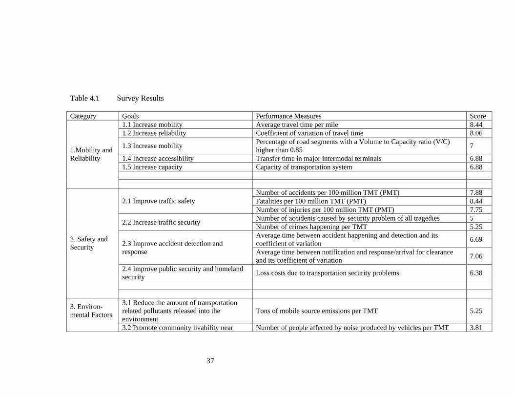
37

Table 4.1 Survey Results Category Goals Performance Measures Score

1.1 Increase mobility Average travel time per mile 8.44 1.2 Increase reliability Coefficient of variation of travel time 8.06

1.3 Increase mobility Percentage of road segments with a Volume to Capacity ratio (V/C) higher than 0.85 7

1.4 Increase accessibility Transfer time in major intermodal terminals 6.88 1.5 Increase capacity Capacity of transportation system 6.88

1.Mobility and Reliability

Number of accidents per 100 million TMT (PMT) 7.88 Fatalities per 100 million TMT (PMT) 8.44 2.1 Improve traffic safety Number of injuries per 100 million TMT (PMT) 7.75 Number of accidents caused by security problem of all tragedies 5 2.2 Increase traffic security Number of crimes happening per TMT 5.25 Average time between accident happening and detection and its coefficient of variation 6.69 2.3 Improve accident detection and

response Average time between notification and response/arrival for clearance and its coefficient of variation 7.06

2.4 Improve public security and homeland security Loss costs due to transportation security problems 6.38

2. Safety and Security

3.1 Reduce the amount of transportation related pollutants released into the environment

Tons of mobile source emissions per TMT 5.25 3. Environ-mental Factors

3.2 Promote community livability near Number of people affected by noise produced by vehicles per TMT 3.81

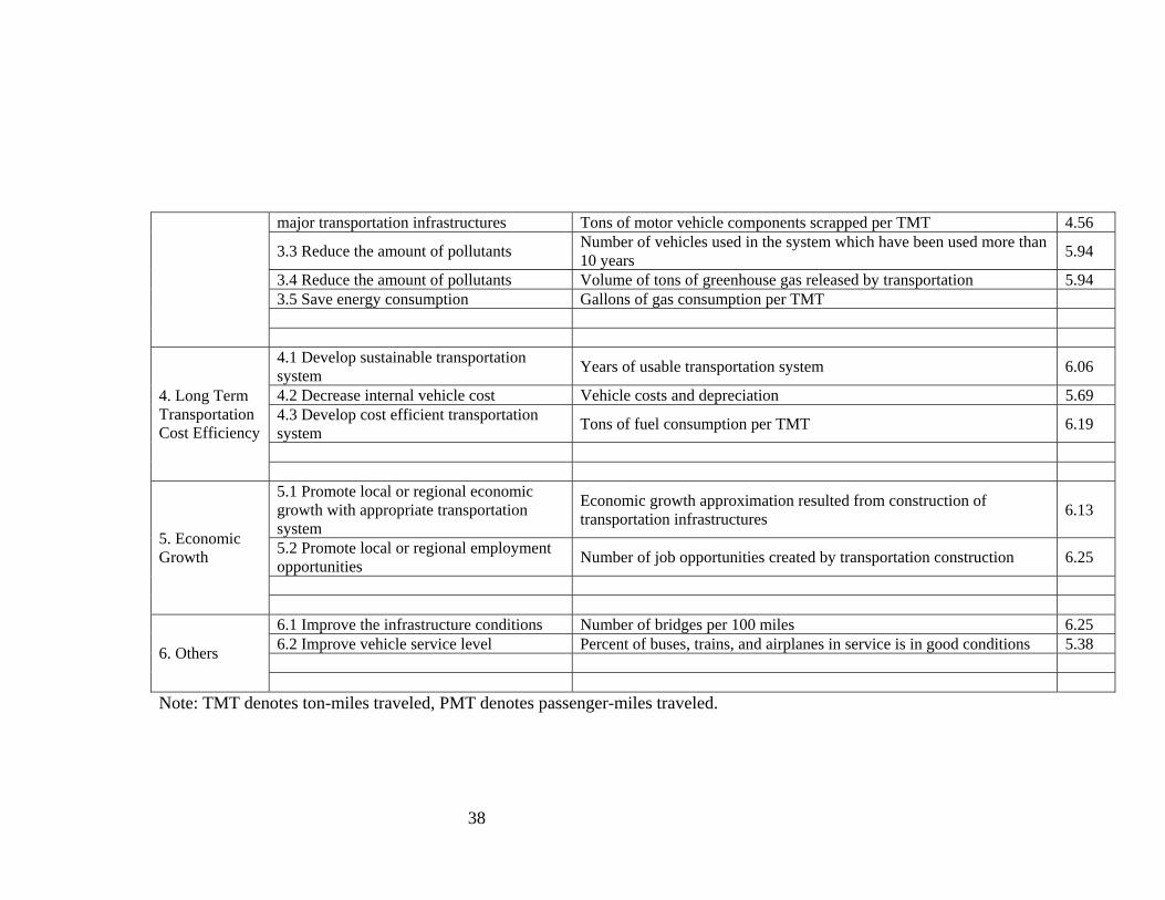
38

major transportation infrastructures Tons of motor vehicle components scrapped per TMT 4.56

3.3 Reduce the amount of pollutants Number of vehicles used in the system which have been used more than 10 years 5.94

3.4 Reduce the amount of pollutants Volume of tons of greenhouse gas released by transportation 5.94 3.5 Save energy consumption Gallons of gas consumption per TMT 4.1 Develop sustainable transportation system Years of usable transportation system 6.06

4.2 Decrease internal vehicle cost Vehicle costs and depreciation 5.69 4.3 Develop cost efficient transportation system Tons of fuel consumption per TMT 6.19

4. Long Term Transportation Cost Efficiency

5.1 Promote local or regional economic growth with appropriate transportation system

Economic growth approximation resulted from construction of transportation infrastructures 6.13

5.2 Promote local or regional employment opportunities Number of job opportunities created by transportation construction 6.25

5. Economic Growth

6.1 Improve the infrastructure conditions Number of bridges per 100 miles 6.25 6.2 Improve vehicle service level Percent of buses, trains, and airplanes in service is in good conditions 5.38 6. Others

Note: TMT denotes ton-miles traveled, PMT denotes passenger-miles traveled.

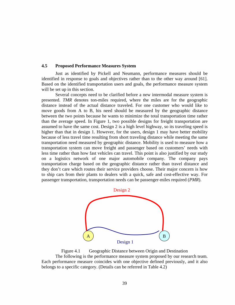
39

4.5 Proposed Performance Measures System Just as identified by Pickell and Neumann, performance measures should be

identified in response to goals and objectives rather than to the other way around [61]. Based on the identified transportation users and goals, the performance measure system will be set up in this section.

Several concepts need to be clarified before a new intermodal measure system is presented. TMR denotes ton-miles required, where the miles are for the geographic distance instead of the actual distance traveled. For one customer who would like to move goods from A to B, his need should be measured by the geographic distance between the two points because he wants to minimize the total transportation time rather than the average speed. In Figure 1, two possible designs for freight transportation are assumed to have the same cost. Design 2 is a high level highway, so its traveling speed is higher than that in design 1. However, for the users, design 1 may have better mobility because of less travel time resulting from short traveling distance while meeting the same transportation need measured by geographic distance. Mobility is used to measure how a transportation system can move freight and passenger based on customers’ needs with less time rather than how fast vehicles can travel. This point is also justified by our study on a logistics network of one major automobile company. The company pays transportation charge based on the geographic distance rather than travel distance and they don’t care which routes their service providers choose. Their major concern is how to ship cars from their plants to dealers with a quick, safe and cost-effective way. For passenger transportation, transportation needs can be passenger-miles required (PMR).

Figure 4.1 Geographic Distance between Origin and Destination

The following is the performance measure system proposed by our research team. Each performance measure coincides with one objective defined previously, and it also belongs to a specific category. (Details can be referred in Table 4.2)

A B Design 1

Design 2

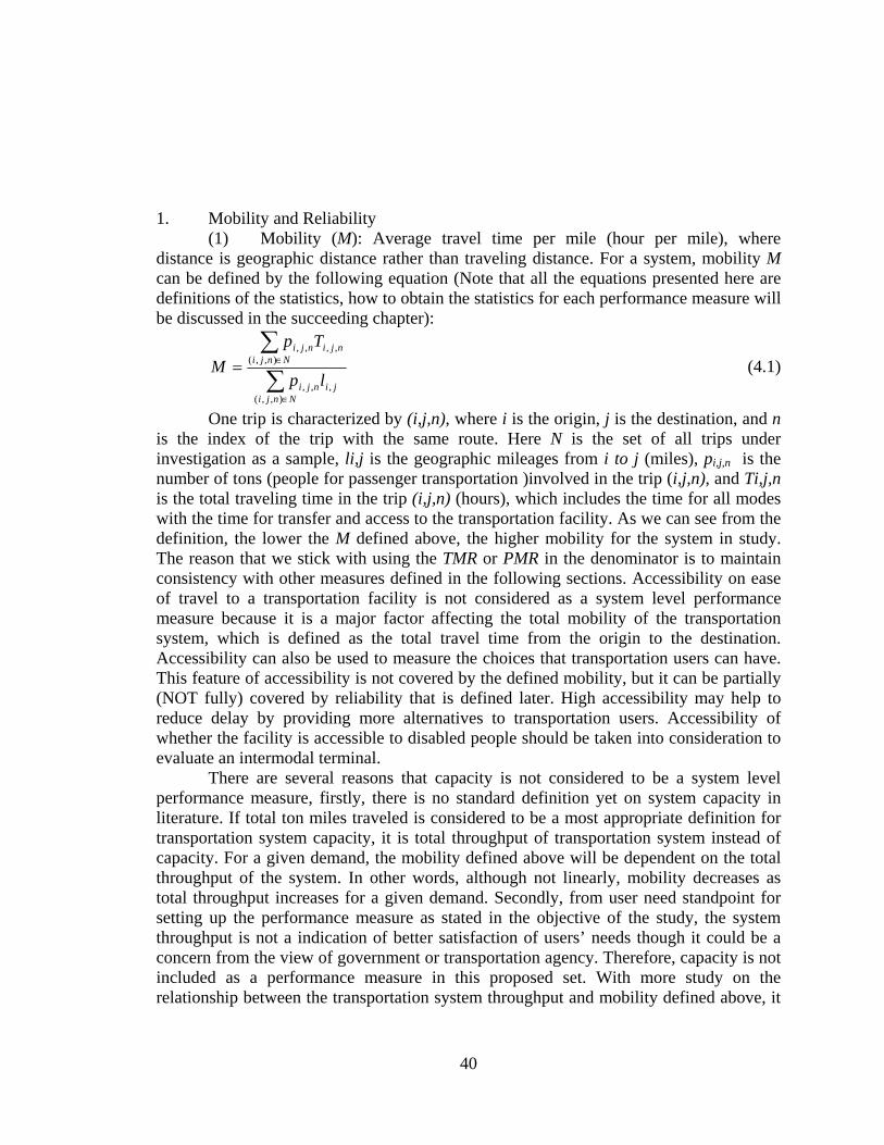
40

1. Mobility and Reliability (1) Mobility (M): Average travel time per mile (hour per mile), where

distance is geographic distance rather than traveling distance. For a system, mobility M can be defined by the following equation (Note that all the equations presented here are definitions of the statistics, how to obtain the statistics for each performance measure will be discussed in the succeeding chapter):

∑∑

∈

∈=

Nnjijinji

Nnjinjinji

lp

TpM

),,(,,,

),,(,,,,

(4.1)

One trip is characterized by (i,j,n), where i is the origin, j is the destination, and n is the index of the trip with the same route. Here N is the set of all trips under investigation as a sample, li,j is the geographic mileages from i to j (miles), pi,j,n is the number of tons (people for passenger transportation )involved in the trip (i,j,n), and Ti,j,n is the total traveling time in the trip (i,j,n) (hours), which includes the time for all modes with the time for transfer and access to the transportation facility. As we can see from the definition, the lower the M defined above, the higher mobility for the system in study. The reason that we stick with using the TMR or PMR in the denominator is to maintain consistency with other measures defined in the following sections. Accessibility on ease of travel to a transportation facility is not considered as a system level performance measure because it is a major factor affecting the total mobility of the transportation system, which is defined as the total travel time from the origin to the destination. Accessibility can also be used to measure the choices that transportation users can have. This feature of accessibility is not covered by the defined mobility, but it can be partially (NOT fully) covered by reliability that is defined later. High accessibility may help to reduce delay by providing more alternatives to transportation users. Accessibility of whether the facility is accessible to disabled people should be taken into consideration to evaluate an intermodal terminal.

There are several reasons that capacity is not considered to be a system level performance measure, firstly, there is no standard definition yet on system capacity in literature. If total ton miles traveled is considered to be a most appropriate definition for transportation system capacity, it is total throughput of transportation system instead of capacity. For a given demand, the mobility defined above will be dependent on the total throughput of the system. In other words, although not linearly, mobility decreases as total throughput increases for a given demand. Secondly, from user need standpoint for setting up the performance measure as stated in the objective of the study, the system throughput is not a indication of better satisfaction of users’ needs though it could be a concern from the view of government or transportation agency. Therefore, capacity is not included as a performance measure in this proposed set. With more study on the relationship between the transportation system throughput and mobility defined above, it

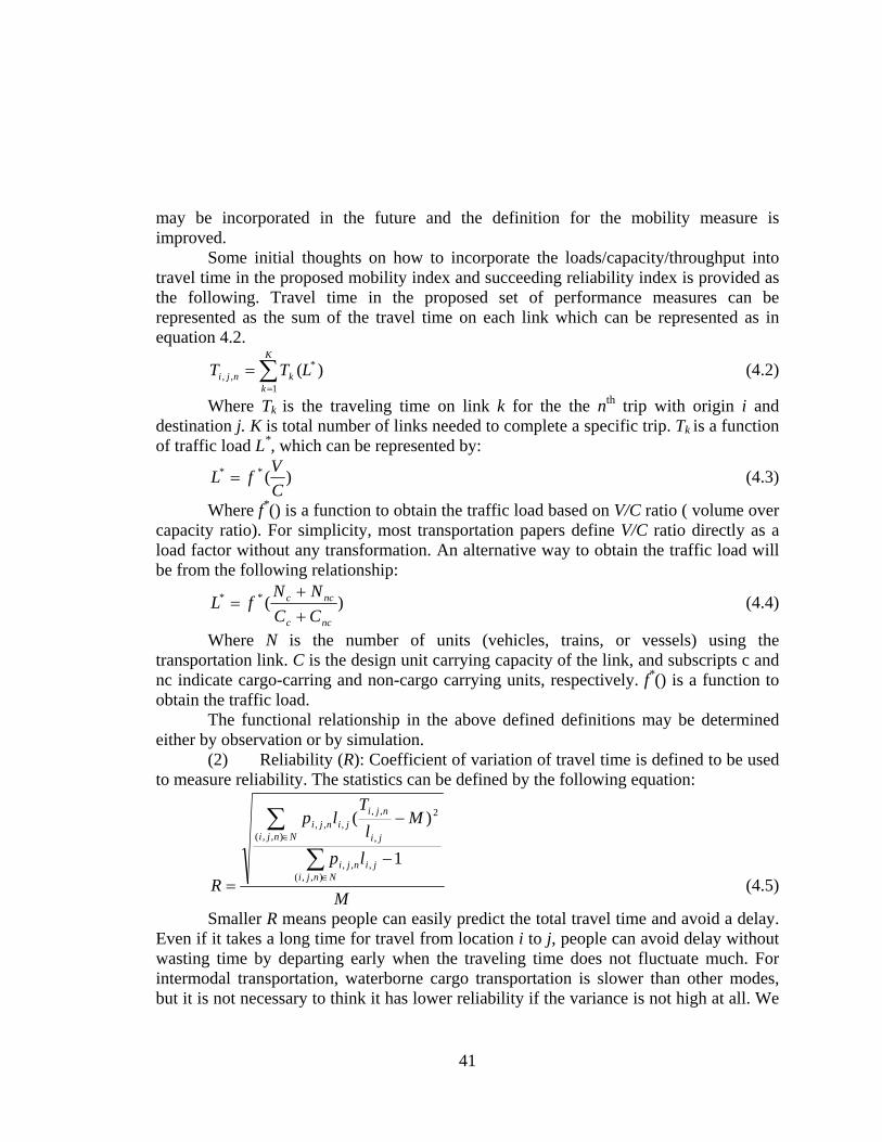
41

may be incorporated in the future and the definition for the mobility measure is improved.

Some initial thoughts on how to incorporate the loads/capacity/throughput into travel time in the proposed mobility index and succeeding reliability index is provided as the following. Travel time in the proposed set of performance measures can be represented as the sum of the travel time on each link which can be represented as in equation 4.2.

)( *

1,, LTT

K

kknji ∑

=

= (4.2)

Where Tk is the traveling time on link k for the the nth trip with origin i and destination j. K is total number of links needed to complete a specific trip. Tk is a function of traffic load L*, which can be represented by:

)(**

CVfL = (4.3)

Where f*() is a function to obtain the traffic load based on V/C ratio ( volume over capacity ratio). For simplicity, most transportation papers define V/C ratio directly as a load factor without any transformation. An alternative way to obtain the traffic load will be from the following relationship:

)(**

ncc

ncc

CCNN

fL++

= (4.4)

Where N is the number of units (vehicles, trains, or vessels) using the transportation link. C is the design unit carrying capacity of the link, and subscripts c and nc indicate cargo-carring and non-cargo carrying units, respectively. f*() is a function to obtain the traffic load.

The functional relationship in the above defined definitions may be determined either by observation or by simulation.

(2) Reliability (R): Coefficient of variation of travel time is defined to be used to measure reliability. The statistics can be defined by the following equation:

M

lp

Ml

Tlp

R Nnjijinji

Nnji ji

njijinji

1

)(

),,(,,,

),,(

2

,

,,,,,

−

−

=∑

∑

∈

∈

(4.5)

Smaller R means people can easily predict the total travel time and avoid a delay. Even if it takes a long time for travel from location i to j, people can avoid delay without wasting time by departing early when the traveling time does not fluctuate much. For intermodal transportation, waterborne cargo transportation is slower than other modes, but it is not necessary to think it has lower reliability if the variance is not high at all. We

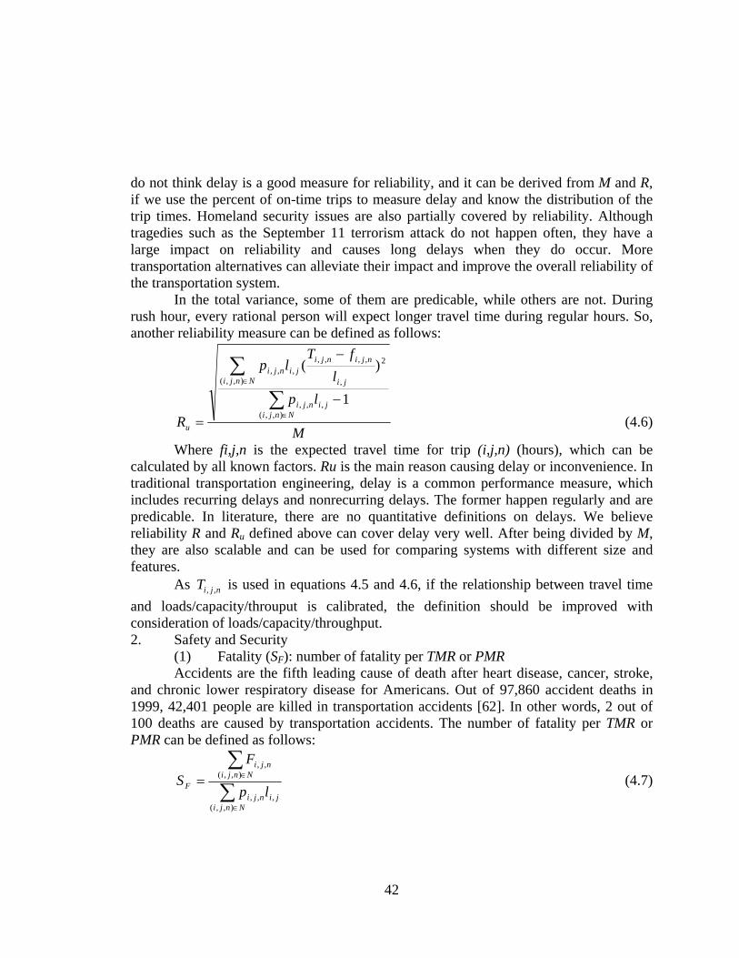
42

do not think delay is a good measure for reliability, and it can be derived from M and R, if we use the percent of on-time trips to measure delay and know the distribution of the trip times. Homeland security issues are also partially covered by reliability. Although tragedies such as the September 11 terrorism attack do not happen often, they have a large impact on reliability and causes long delays when they do occur. More transportation alternatives can alleviate their impact and improve the overall reliability of the transportation system.

In the total variance, some of them are predicable, while others are not. During rush hour, every rational person will expect longer travel time during regular hours. So, another reliability measure can be defined as follows:

M

lpl

fTlp

R Nnjijinji

Nnji ji

njinjijinji

u

1

)(

),,(,,,

),,(

2

,

,,,,,,,

−

−

=∑

∑

∈

∈

(4.6)

Where fi,j,n is the expected travel time for trip (i,j,n) (hours), which can be calculated by all known factors. Ru is the main reason causing delay or inconvenience. In traditional transportation engineering, delay is a common performance measure, which includes recurring delays and nonrecurring delays. The former happen regularly and are predicable. In literature, there are no quantitative definitions on delays. We believe reliability R and Ru defined above can cover delay very well. After being divided by M, they are also scalable and can be used for comparing systems with different size and features.

As njiT ,, is used in equations 4.5 and 4.6, if the relationship between travel time and loads/capacity/throuput is calibrated, the definition should be improved with consideration of loads/capacity/throughput. 2. Safety and Security

(1) Fatality (SF): number of fatality per TMR or PMR Accidents are the fifth leading cause of death after heart disease, cancer, stroke,

and chronic lower respiratory disease for Americans. Out of 97,860 accident deaths in 1999, 42,401 people are killed in transportation accidents [62]. In other words, 2 out of 100 deaths are caused by transportation accidents. The number of fatality per TMR or PMR can be defined as follows:

∑∑

∈

∈=

Nnjijinji

Nnjinji

F lp

FS

),,(,,,

),,(,,

(4.7)

43

Here, Fi,j,n is the number of fatalities for trip (i,j,n), li,j is the actual distance traveled between origin i and destination j. The fatality rate for different modes in urban and rural areas is depicted in Figure 4.2 [63].

Figure 4.2 Fatalities for Different Modes in Urban and Rural Areas

(2) Injury Rate (SI): Number of injuries per TMR or PMR The accident outcomes for different modes are different. An airplane crash may

result in more fatalities rather than injuries than other modes. Similarly, the number of injuries can be defined as follows:

∑∑

∈

∈=

Nnjijinji

Nnjinji

I lp

IS

),,(,,,

),,(,,

(4.8)

Here, Ii,j,n is the number of injuries for trip (i,j,n). Both SF and SI are some of the costs for transportation systems. Safety also has a large impact on delay and Lindley [59] estimates that over 60 percent of the congestion delay experienced on urban freeways is due to accidents rather than recurring congestion.

In the literature, accident detection and response efficiency are usually considered a part of safety measure. Though it influences the outcomes of accidents, it has already been covered by mobility and reliability. The above fatality and injury rate does not consider the loss of congestion caused by accidents.

(3) Property Damage (Sp): Property damage cost per TMR or PMR Besides the loss of human lives and health, accidents can also result in property

damage. We use Sp to capture this effect:

∑∑

∈

∈=

Nnjijinji

Nnjinji

p lp

DS

),,(,,,

),,(,,

(4.9)

Here, Di,j,n is property damage cost caused by accidents in trip (i,j,n) (dollars).

Urban & Rural Transport Fatality Rates: 1990-95

0 0.25

0.5 0.75

1 1.25

1.5 1.75

Auto & Truck School Bus Trolley Bus Trasnit

Motor BusLight Rail Metro Commuter

Rail

Fatalities per 100 Million Passenger Miles

44

In the literature, accident detection and response efficiency are usually considered a part of safety measure. Though it influences the outcomes of accidents, it is already covered by mobility and reliability. The above fatality rate and injury rate doesn’t consider the loss of congestion caused by accidents. 3. Environmental Impact

A transportation system has a big impact on environment and, as a result, vehicle pollution and energy consumption have got more and more attention in transportation system analysis and in the transportation planning process. The main measures we identify are transportation related pollutants released and community livability near major transportation infrastructures. Other issues such as the impact of large constructed transportation project on fragmentation of habitat and wildlife ecology, and water pollution should also be a consideration. However, theses impacts are hard to quantify and they are not developed in the proposed performance measure set yet.

(1) Transportation related pollutants released (P): Tons of mobile source emissions from transportation systems per TMR or PMR, which can be obtained by

∑∑

∈

∈=

Nnjijinji

Nnjinji

lp

POP

),,(,,,

),,(,,

(4.10)

where, POi,j,n is the tons of mobile pollutants emissions involved in trip (i,j,n) (tons). The main emissions include carbon dioxide, carbon monoxide, nitrogen oxides, organic compounds, sulfur dioxide, and lead. Transportation is the main contributor to these air pollutants. For example, the transportation share of total carbon monoxide emission is 70% and that of carbon dioxide is 30%. These emissions can cause health problem, acid rain, global warming, and other damage. Under this systematic measure, we can develop a measure for each pollutant.

(2) Community livability (L): percent of people affected by transportation systems

A transportation system can result in an increase in noise, can influence animal migration, and other issues. For example, one community may be against having an airport in the neighborhood. Though the impact on the community is pretty subjective, we can use survey to figure out the percent of people who think they are negatively impacted by transportation systems for a particular region. We should notice here we do not use TMR or PMR as denominator, because L is not from the passengers or freight viewpoint, but from the community or society viewpoint.

T

a

PP

L = (4.11)

45

where, Pa denotes the number of people that are negatively affected by transportation systems. PT denotes total number of people using the transportation system. 4. Long Term Transportation Cost Efficiency

Here, only the direct cost of a transportation system is considered rather than a comprehensive one, which includes the external impact like environment issue or influence on community livability. The direct cost includes vehicle operation cost, construction, operation, maintenance, and disposal for transportation facilities.

(1) Vehicle Operation Cost (VC): Vehicle operation cost mainly includes cost of fuel consumption, cost for vehicle insurance, cost for vehicle maintenance, and cost for vehicle aging per TMR or PMR. This general cost index will consider the life cycle cost for vehicle operation and may vary for different modes of the transportation system. In order to evaluate the whole system, different components of transportation mode should be taken into consideration for each segment of the trip. The statistics for vehicle operation cost can be defined by the following formula:

∑∑

∈

∈

++++=

Nnjijinji

Nnjinjinjinjinjinji

lp

VOVAVMVIGCVC

),,(,,,

),,(,,,,,,,,,, )(

(4.12)

GCi,j,n is the fuel consumption cost involved in trip (i,j,n) (dollars). VIi,j,n is the vehicle insurance cost involved in trip (i,j,n) (dollars). VMi,j,n is the vehicle maintenance cost involved in trip (i,j,n) (dollars). VAi,j,n is the associated cost with vehicle aging in its life cycle involved in trip (i,j,n) (dollars). njiVO ,, is the other associated cost in its life cycle involved in trip (i,j,n) (dollars).

(2) Transportation Facility Cost (FC): the cost of the transportation facility per TMR or PMR. Since transportation system may be designed to operate for decades and a different type of cost is incurred in different stages of its life cycle, a money flow diagram and interest issue should be considered to get the average cost per TMR or PMR. Figure 4.3 is an example of money flow for a transportation system, which has a 20-year life cycle. The first three years are for design and construction. At the end of the life cycle, there are some disposal costs to get rid of the old system.

Figure 4.3 Money Flow Diagram for a Transportation System

1 2 3 4 5 17 18 19 20

15M

50M 50M

5M 5M 5M 5M 5M 5M

10M

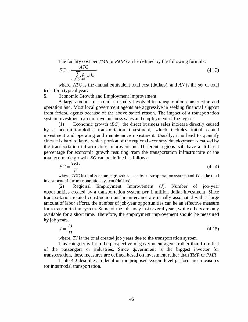
46

The facility cost per TMR or PMR can be defined by the following formula:

∑∈

=

ANnjijinji lp

ATCFC

),,(,,,

(4.13)

where, ATC is the annual equivalent total cost (dollars), and AN is the set of total trips for a typical year. 5. Economic Growth and Employment Improvement

A large amount of capital is usually involved in transportation construction and operation and. Most local government agents are aggressive in seeking financial support from federal agents because of the above stated reason. The impact of a transportation system investment can improve business sales and employment of the region.

(1) Economic growth (EG): the direct business sales increase directly caused by a one-million-dollar transportation investment, which includes initial capital investment and operating and maintenance investment. Usually, it is hard to quantify since it is hard to know which portion of the regional economy development is caused by the transportation infrastructure improvements. Different regions will have a different percentage for economic growth resulting from the transportation infrastructure of the total economic growth. EG can be defined as follows:

TITEGEG = (4.14)

where, TEG is total economic growth caused by a transportation system and TI is the total investment of the transportation system (dollars).

(2) Regional Employment Improvement (J): Number of job-year opportunities created by a transportation system per 1 million dollar investment. Since transportation related construction and maintenance are usually associated with a large amount of labor efforts, the number of job-year opportunities can be an effective measure for a transportation system. Some of the jobs may last several years, while others are only available for a short time. Therefore, the employment improvement should be measured by job years.

TITJJ = (4.15)

where, TJ is the total created job years due to the transportation system. This category is from the perspective of government agents rather than from that

of the passengers or industries. Since government is the biggest investor for transportation, these measures are defined based on investment rather than TMR or PMR.

Table 4.2 describes in detail on the proposed system level performance measures for intermodal transportation.

47

4.6 Data Availability Discussion This section discusses the data availability issue for the proposed performance

measure system. Data availability will directly affect how useful the proposed model is. At the same time, whether data are available depends on where the model is applied. Here, some general discussion and recommendations are provided.

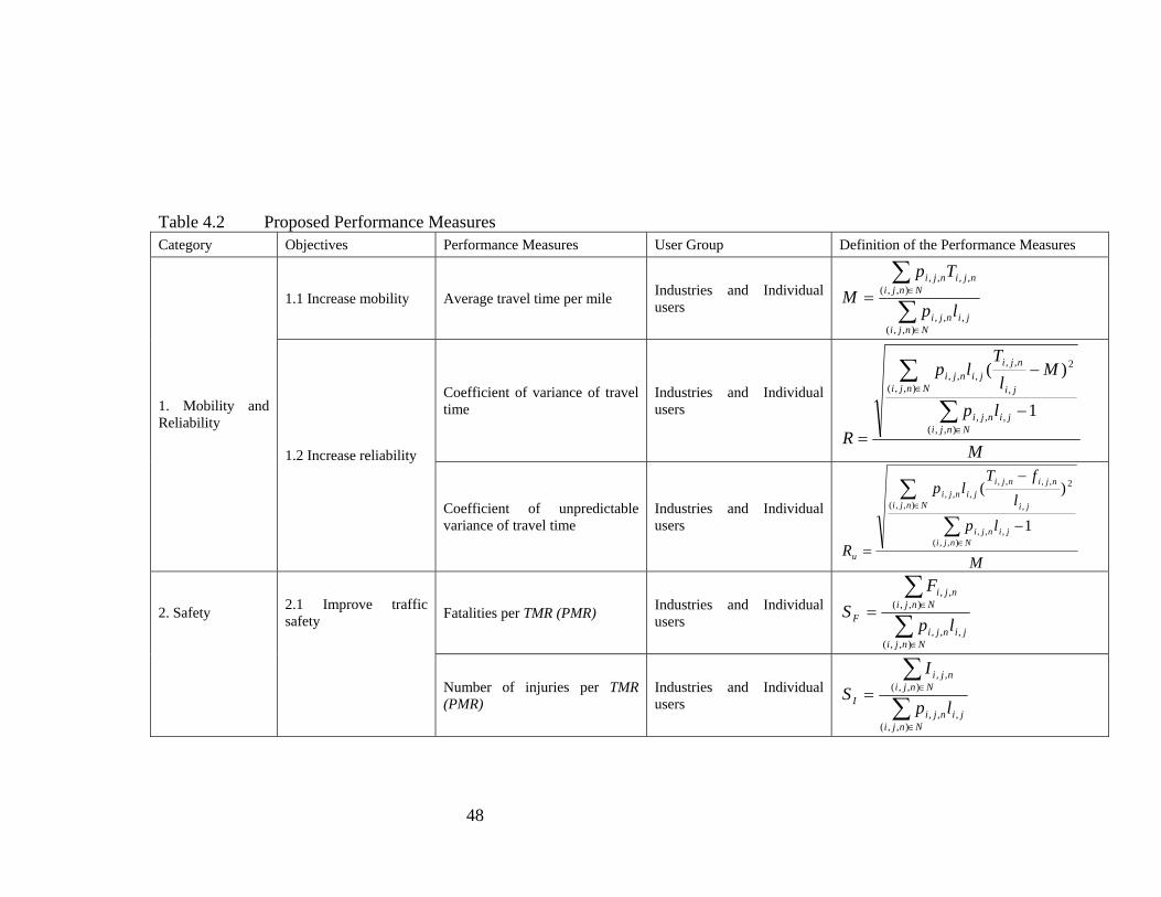
48

Table 4.2 Proposed Performance Measures Category Objectives Performance Measures User Group Definition of the Performance Measures

1.1 Increase mobility Average travel time per mile Industries and Individual users ∑

∑

∈

∈=

Nnjijinji

Nnjinjinji

lp

TpM

),,(,,,

),,(,,,,

Coefficient of variance of travel time

Industries and Individual users

M

lp

Ml

Tlp

R Nnjijinji

Nnji ji

njijinji

1

)(

),,(,,,

),,(

2

,

,,,,,

−

−

=∑

∑

∈

∈

1. Mobility and Reliability

1.2 Increase reliability

Coefficient of unpredictable variance of travel time

Industries and Individual users

M

lpl

fTlp

R Nnjijinji

Nnji ji

njinjijinji

u

1

)(

),,(,,,

),,(

2

,

,,,,,,,

−

−

=∑

∑

∈

∈

Fatalities per TMR (PMR) Industries and Individual users ∑

∑

∈

∈=

Nnjijinji

Nnjinji

F lp

FS

),,(,,,

),,(,,

2. Safety 2.1 Improve traffic safety

Number of injuries per TMR (PMR)

Industries and Individual users ∑

∑

∈

∈=

Nnjijinji

Nnjinji

I lp

IS

),,(,,,

),,(,,

49

Property damage cost per TMR (PMR)

Industries and Individual users ∑

∑

∈

∈=

Nnjijinji

Nnjinji

P lp

DS

),,(,,,

),,(,,

3.1 Reduce pollutants released into the environment

Tons of mobile emissions from on-road motor vehicles per TMR (PMR)

Industries, Society Users, and Individual users ∑

∑

∈

∈=

Nnjijinji

Nnjinji

lp

poP

),,(,,,

),,(,,

3. Environmental Impact 3.2 Promote community

livability near major transportation infrastructures

Percent of people affected by noise produced by vehicles per TMR (PMR)

Industries, Society Users, and Individual users T

a

PP

L =

4.1 Develop cost efficient transportation system

Vehicle operation cost per TMR (PMR)

Industries, Investors, Society Users, and Individual users ∑

∑

∈

∈

++++=

Nnjijinji

Nnjinjinjinjinjinji

lp

VOVAVMVIGCVC

),,(,,,

),,(,,,,,,,,,,

*

)(

4. Long Term Transportation Cost Efficiency 4.2 Save transportation

facility cost Cost of transportation facility per TMR (PMR)

Industries, Investors, and Individual users ∑

∈

=

ANnjijinji lp

ATCFC

),,(,,,

5.1 Promote local or regional economic growth with appropriate transportation system

Economic growth approximation resulted from construction of transportation infrastructures

Society Users TITEGEG =

5. Economic Growth and Employment Improvement 5.2 Promote local or

regional employment opportunities

Number of job opportunities created by transportation system per 1 million dollar investment

Society Users TITJJ =

50

For mobility and reliability indices, O&D data are required to calculate the value of measures. O&D data can be obtained from many statewide or regional transportation planning documents. Another source for O&D data is Commodity Flow Survey data as identified by NCIT and MDOT [65]. Other sources like TRANSEARCH data, Vehicle Inventory and User Survey, and Ground Counts data are also discussed in detail by Zhang, Bowden, and Allen [65]. Travel time can be derived from the traffic assignment results from traditional transportation planning and modeling methods. Different assignment models may be used for different purposes. The numerator in the mobility definition can be obtained by combining the travel time and O&D data. Geographic distances are available through Geographic information system (GIS) related packages. This distance and the O&D data can be combined to get the denominator in the equation. To calculate the reliability index, some historical data have to be collected, and a survey can be conducted in a representative group of people. The cost to perform a survey is high and dependent on how detailed it is. In practice, some available data are based on vehicles instead of tonnages or passengers. A study on average payload or vehicle occupancy is necessary in order to apply the model to a specific problem.

Many states have GIS-based accident information systems, and there are historical data of traffic safety contained in the system. If a smaller scale or region based analysis is required, the data can also be derived from the existing GIS system. Although this system may not be implemented currently in some states, those state DOTs’ have documents containing traffic safety data for every year. With multiple years of data, the accident rate, injury rate, fatality rate, and property damage rate can be derived.

Environment related data can be obtained from various sources. The most popular source is the transportation energy data book distributed by the U.S. Department of Energy. The book is updated regularly, and the newest version is edition 22, published in September 2002 [66]. The book is edited by the Center for Transportation Analysis and Oak Ridge National Laboratory, which is well known for its credible research on environment impacts analysis.

Transportation facility cost and vehicle operation cost can be obtained from some ongoing infrastructure projects or past infrastructure projects. Many DOTs have documents on feasibility analysis of specific transportation infrastructure projects. Each region has its own characteristics including labor cost, raw material cost, transportation cost, etc. These factors have to be addressed in practical application of these performance measures.

Economic growth and employment improvement data can be obtained from the U.S. Census of Bureau [67]. Regional data on economic growth and employment improvement data can also be obtained by the related regional agencies. This effort has to be done with the coordination of the DOTs.

With the emphasis of information technologies applications in transportation research, more data can be obtained than ever before. In California’s PeMS (Performance

51

Measure System) system, historical and real-time data are collected by various ways including sensor and loop detectors. Those data are converted into useful information to improve system management, assist travelers, and challenge the current understanding of freeway traffic behavior [68].

There is further discussion on the data availability and cost analysis related issues in the following chapter. In practical application, more research and study are necessary on the data issue for each category. As we have identified, the data availability in different regions depends on their characteristics and are application specific.

52

CHAPTER V A CASE STUDY FOR PROPOSED PERFORMANCE MEASURES

A case study is conducted to demonstrate how to apply the system-level performance measures. Other potential applications are presented after the case study.

5.1 Introduction The State of Mississippi is chosen as the geographic region for the case study

because some related data are already available for the state. There are totally 82 counties in the state as shown in Figure 5.1 which is generated in TransCAD [69]. The state is divided into the southern region and the northern region as shown in Figure 5.2 for performance comparison between them. There are 44 counties in the northern part of Mississippi and 38 counties in the southern part of Mississippi due to this division (the detailed list of the counties included in each region can be referred in Table 5.1). Their transportation performance in terms of carrying out the within-traffic demand in the state is evaluated based on the proposed performance measures. Highway transportation network in the state is shown in Figure 5.3. The interstate highways are represented by red lines; the U.S. routes are represented by bold blue lines; and the state highways are represented by light blue lines. Figure 5.4 is a visual comparison of the transportation networks of the two regions. Institutively, the southern part of the state has much better transportation infrastructure than the northern part since there are more mileages of high-level highways. Table 5.1 FIPS of Northern and Southern Part in Mississippi County List (FIPS) Total

Northern

28003,28007,28009,28011,28013,28015,28017,28019,28025, 28027,28033,28043,28051,28053,28057,28069,28071,28079, 28081,28083,28087,28093,28095,28097,28099,28103,28105, 28107,28115,28117,28119,28125,28133,28135,28137,28139, 28141,28143,28145,28151, 28155,28159,28161,28163

44 Counties

Southern

2800128005,28021,28023,28029,28031,28035,28037,28039, 28041,28045,28047,28049,28055,28059,28061,28063,28065, 28067,28073,28075,28077,28085,28089,28091,28101,28109, 28111,28113,28121,28123,28127,28129,28131,28147,28149, 28153,28157

38 Counties

53

Figure 5.1 Counties in the State of Mississippi

Figure 5.2 Northern Part of Mississippi and Southern Part of Mississippi

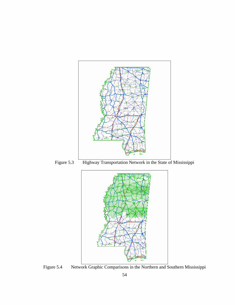
54

Figure 5.3 Highway Transportation Network in the State of Mississippi

Figure 5.4 Network Graphic Comparisons in the Northern and Southern Mississippi

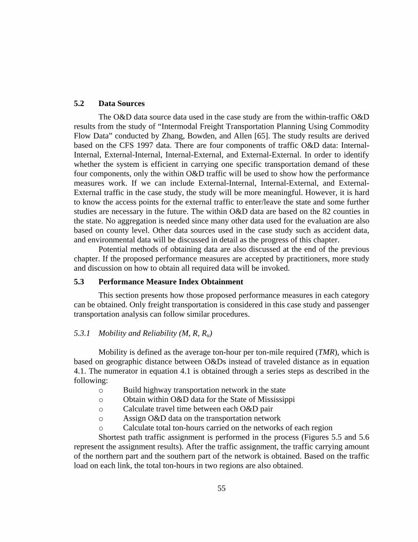
55

5.2 Data Sources The O&D data source data used in the case study are from the within-traffic O&D

results from the study of “Intermodal Freight Transportation Planning Using Commodity Flow Data” conducted by Zhang, Bowden, and Allen [65]. The study results are derived based on the CFS 1997 data. There are four components of traffic O&D data: Internal-Internal, External-Internal, Internal-External, and External-External. In order to identify whether the system is efficient in carrying one specific transportation demand of these four components, only the within O&D traffic will be used to show how the performance measures work. If we can include External-Internal, Internal-External, and External-External traffic in the case study, the study will be more meaningful. However, it is hard to know the access points for the external traffic to enter/leave the state and some further studies are necessary in the future. The within O&D data are based on the 82 counties in the state. No aggregation is needed since many other data used for the evaluation are also based on county level. Other data sources used in the case study such as accident data, and environmental data will be discussed in detail as the progress of this chapter.

Potential methods of obtaining data are also discussed at the end of the previous chapter. If the proposed performance measures are accepted by practitioners, more study and discussion on how to obtain all required data will be invoked.

5.3 Performance Measure Index Obtainment This section presents how those proposed performance measures in each category

can be obtained. Only freight transportation is considered in this case study and passenger transportation analysis can follow similar procedures.

5.3.1 Mobility and Reliability (M, R, Ru)

Mobility is defined as the average ton-hour per ton-mile required (TMR), which is based on geographic distance between O&Ds instead of traveled distance as in equation 4.1. The numerator in equation 4.1 is obtained through a series steps as described in the following:

o Build highway transportation network in the state o Obtain within O&D data for the State of Mississippi o Calculate travel time between each O&D pair o Assign O&D data on the transportation network o Calculate total ton-hours carried on the networks of each region Shortest path traffic assignment is performed in the process (Figures 5.5 and 5.6

represent the assignment results). After the traffic assignment, the traffic carrying amount of the northern part and the southern part of the network is obtained. Based on the traffic load on each link, the total ton-hours in two regions are also obtained.

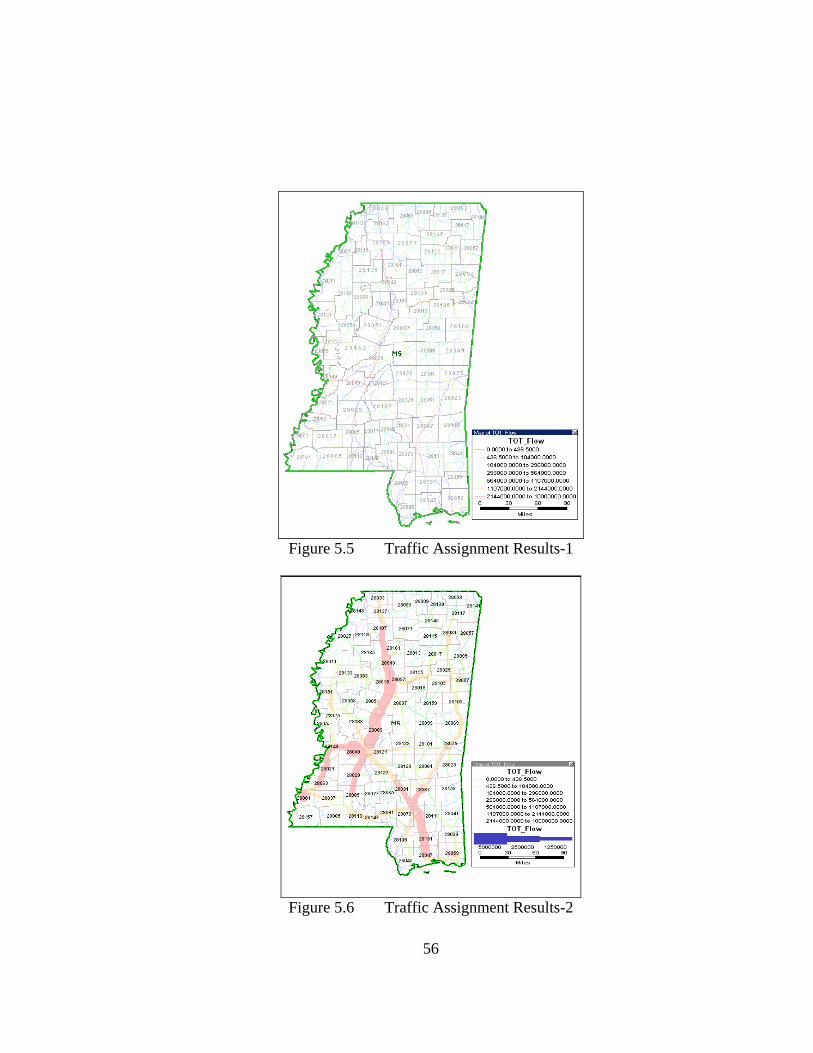
56

Figure 5.5 Traffic Assignment Results-1

Figure 5.6 Traffic Assignment Results-2

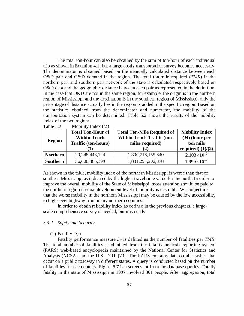
57

The total ton-hour can also be obtained by the sum of ton-hour of each individual trip as shown in Equation 4.1, but a large costly transportation survey becomes necessary. The denominator is obtained based on the manually calculated distance between each O&D pair and O&D demand in the region. The total ton-mile required (TMR) in the northern part and southern part network of the state is calculated respectively based on O&D data and the geographic distance between each pair as represented in the definition. In the case that O&D are not in the same region, for example, the origin is in the northern region of Mississippi and the destination is in the southern region of Mississippi, only the percentage of distance actually lies in the region is added to the specific region. Based on the statistics obtained from the denominator and numerator, the mobility of the transportation system can be determined. Table 5.2 shows the results of the mobility index of the two regions. Table 5.2 Mobility Index (M)

Region

Total Ton-Hour of Within-Truck

Traffic (ton-hours) (1)

Total Ton-Mile Required of Within-Truck Traffic (ton-

miles required) (2)

Mobility Index (M) (hour per

ton mile required) (1)/(2)

Northern 29,248,448,124 1,390,718,155,840 210103.2 −× Southern 36,608,365,399 1,831,294,202,878 210999.1 −×

As shown in the table, mobility index of the northern Mississippi is worse than that of southern Mississippi as indicated by the higher travel time value for the north. In order to improve the overall mobility of the State of Mississippi, more attention should be paid to the northern region if equal development level of mobility is desirable. We conjecture that the worse mobility in the northern Mississippi may be caused by the low accessibility to high-level highway from many northern counties.

In order to obtain reliability index as defined in the previous chapters, a large-scale comprehensive survey is needed, but it is costly.

5.3.2 Safety and Security

(1) Fatality (SF) Fatality performance measure SF is defined as the number of fatalities per TMR.

The total number of fatalities is obtained from the fatality analysis reporting system (FARS) web-based encyclopedia maintained by the National Center for Statistics and Analysis (NCSA) and the U.S. DOT [70]. The FARS contains data on all crashes that occur on a public roadway in different states. A query is conducted based on the number of fatalities for each county. Figure 5.7 is a screenshot from the database queries. Totally fatality in the state of Mississippi in 1997 involved 861 people. After aggregation, total

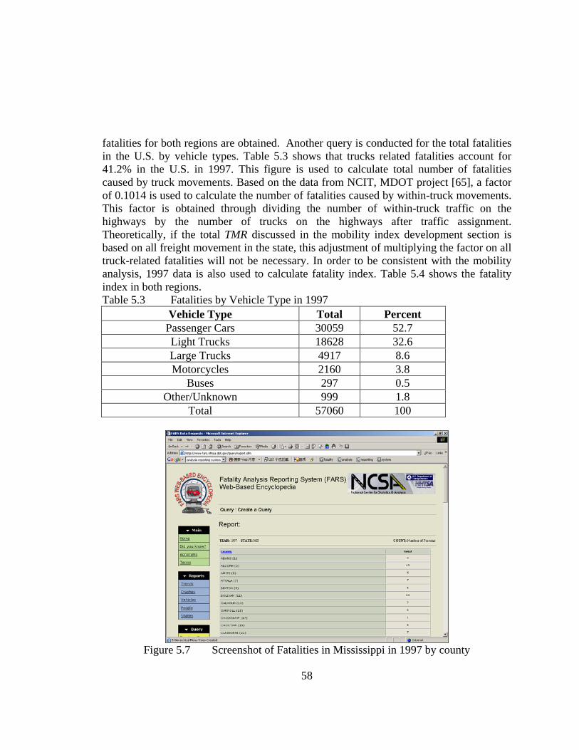
58

fatalities for both regions are obtained. Another query is conducted for the total fatalities in the U.S. by vehicle types. Table 5.3 shows that trucks related fatalities account for 41.2% in the U.S. in 1997. This figure is used to calculate total number of fatalities caused by truck movements. Based on the data from NCIT, MDOT project [65], a factor of 0.1014 is used to calculate the number of fatalities caused by within-truck movements. This factor is obtained through dividing the number of within-truck traffic on the highways by the number of trucks on the highways after traffic assignment. Theoretically, if the total TMR discussed in the mobility index development section is based on all freight movement in the state, this adjustment of multiplying the factor on all truck-related fatalities will not be necessary. In order to be consistent with the mobility analysis, 1997 data is also used to calculate fatality index. Table 5.4 shows the fatality index in both regions. Table 5.3 Fatalities by Vehicle Type in 1997

Vehicle Type Total Percent Passenger Cars 30059 52.7 Light Trucks 18628 32.6 Large Trucks 4917 8.6 Motorcycles 2160 3.8

Buses 297 0.5 Other/Unknown 999 1.8

Total 57060 100

Figure 5.7 Screenshot of Fatalities in Mississippi in 1997 by county

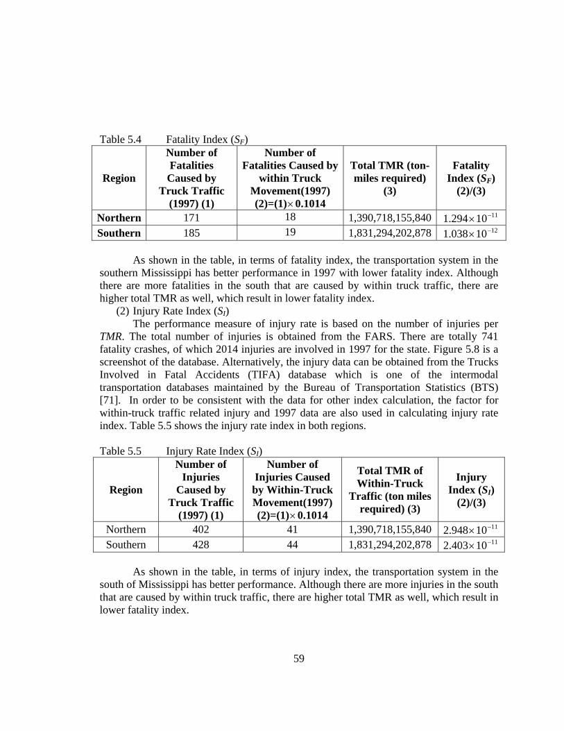
59

Table 5.4 Fatality Index (SF)

Region

Number of Fatalities

Caused by Truck Traffic

(1997) (1)

Number of Fatalities Caused by

within Truck Movement(1997) (2)=(1)×0.1014

Total TMR (ton-miles required)

(3)

Fatality Index (SF)

(2)/(3)

Northern 171 18 1,390,718,155,840 1110294.1 −×

Southern 185 19 1,831,294,202,878 1210038.1 −×

As shown in the table, in terms of fatality index, the transportation system in the southern Mississippi has better performance in 1997 with lower fatality index. Although there are more fatalities in the south that are caused by within truck traffic, there are higher total TMR as well, which result in lower fatality index.

(2) Injury Rate Index (SI) The performance measure of injury rate is based on the number of injuries per

TMR. The total number of injuries is obtained from the FARS. There are totally 741 fatality crashes, of which 2014 injuries are involved in 1997 for the state. Figure 5.8 is a screenshot of the database. Alternatively, the injury data can be obtained from the Trucks Involved in Fatal Accidents (TIFA) database which is one of the intermodal transportation databases maintained by the Bureau of Transportation Statistics (BTS) [71]. In order to be consistent with the data for other index calculation, the factor for within-truck traffic related injury and 1997 data are also used in calculating injury rate index. Table 5.5 shows the injury rate index in both regions.

Table 5.5 Injury Rate Index (SI)

Region

Number of Injuries

Caused by Truck Traffic

(1997) (1)

Number of Injuries Caused by Within-Truck Movement(1997) (2)=(1)×0.1014

Total TMR of Within-Truck

Traffic (ton miles required) (3)

Injury Index (SI)

(2)/(3)

Northern 402 41 1,390,718,155,840 2.948 1110−×

Southern 428 44 1,831,294,202,878 2.403 1110−×

As shown in the table, in terms of injury index, the transportation system in the south of Mississippi has better performance. Although there are more injuries in the south that are caused by within truck traffic, there are higher total TMR as well, which result in lower fatality index.

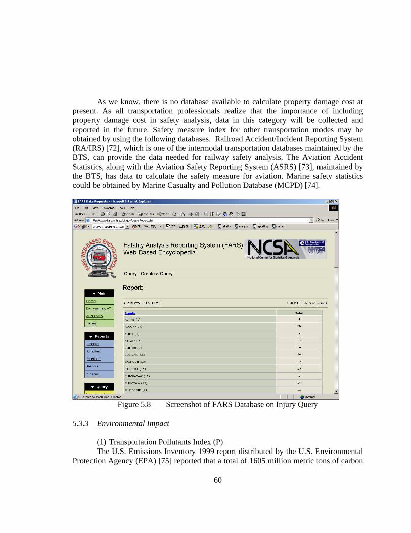
60

As we know, there is no database available to calculate property damage cost at present. As all transportation professionals realize that the importance of including property damage cost in safety analysis, data in this category will be collected and reported in the future. Safety measure index for other transportation modes may be obtained by using the following databases. Railroad Accident/Incident Reporting System (RA/IRS) [72], which is one of the intermodal transportation databases maintained by the BTS, can provide the data needed for railway safety analysis. The Aviation Accident Statistics, along with the Aviation Safety Reporting System (ASRS) [73], maintained by the BTS, has data to calculate the safety measure for aviation. Marine safety statistics could be obtained by Marine Casualty and Pollution Database (MCPD) [74].

Figure 5.8 Screenshot of FARS Database on Injury Query

5.3.3 Environmental Impact

(1) Transportation Pollutants Index (P) The U.S. Emissions Inventory 1999 report distributed by the U.S. Environmental

Protection Agency (EPA) [75] reported that a total of 1605 million metric tons of carbon

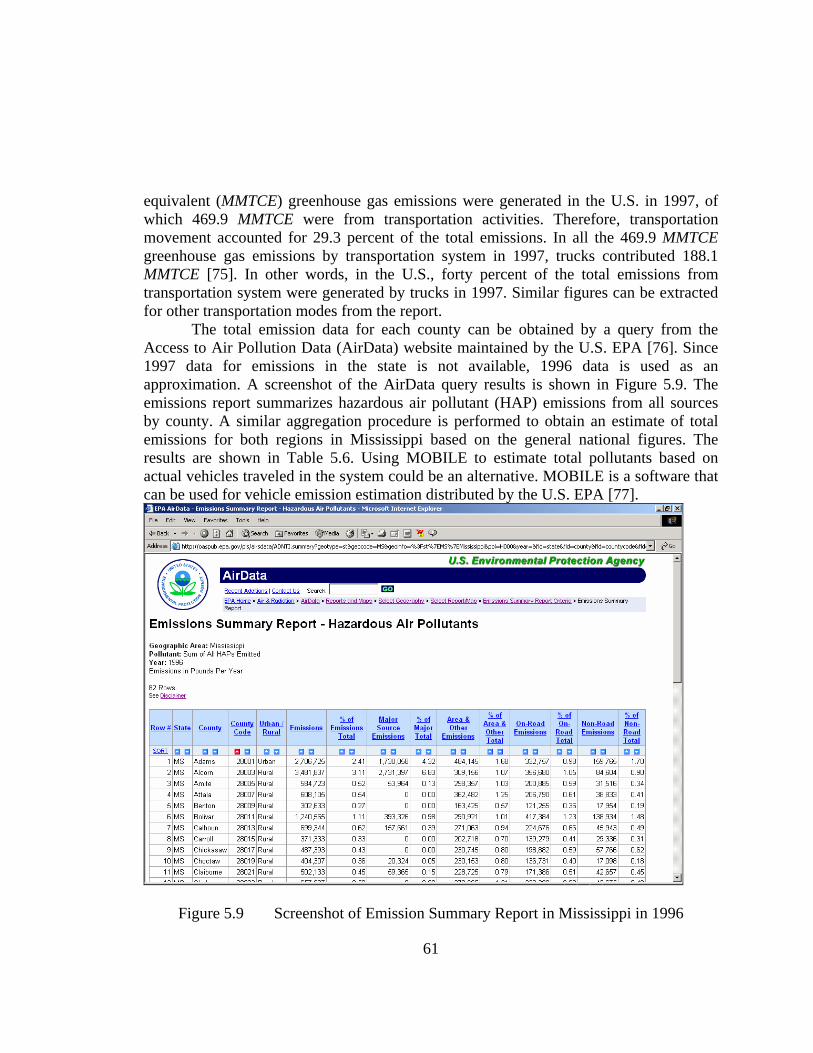
61

equivalent (MMTCE) greenhouse gas emissions were generated in the U.S. in 1997, of which 469.9 MMTCE were from transportation activities. Therefore, transportation movement accounted for 29.3 percent of the total emissions. In all the 469.9 MMTCE greenhouse gas emissions by transportation system in 1997, trucks contributed 188.1 MMTCE [75]. In other words, in the U.S., forty percent of the total emissions from transportation system were generated by trucks in 1997. Similar figures can be extracted for other transportation modes from the report.

The total emission data for each county can be obtained by a query from the Access to Air Pollution Data (AirData) website maintained by the U.S. EPA [76]. Since 1997 data for emissions in the state is not available, 1996 data is used as an approximation. A screenshot of the AirData query results is shown in Figure 5.9. The emissions report summarizes hazardous air pollutant (HAP) emissions from all sources by county. A similar aggregation procedure is performed to obtain an estimate of total emissions for both regions in Mississippi based on the general national figures. The results are shown in Table 5.6. Using MOBILE to estimate total pollutants based on actual vehicles traveled in the system could be an alternative. MOBILE is a software that can be used for vehicle emission estimation distributed by the U.S. EPA [77].

Figure 5.9 Screenshot of Emission Summary Report in Mississippi in 1996

62

Table 5.6 Transportation Pollutants Index (P)

Region

Total Pollutants Generated by

Freight Transportation (1996, tons) (1)

Total Pollutants Generated by Within-Truck Traffic (1996,

tons) (2)=(1) 1014.0×

Total TMR (ton miles required)

(3)

Transportation Pollutants Index (P) (tons per ton mile required)

(2)/(3)

Northern 2824.637 286.418 1,390,718,155,840 1010059.2 −× Southern 3744.575 379.700 1,831,294,202,878 1010073.2 −×

In terms of transportation environment impact, the northern transportation system

has better performance with lower transportation pollutants index. There is no existing data source to calculate the community livability index and a

survey may be necessary. To do the survey, both the sample size and the sample source should be carefully determined along with well-designed survey methods and questionnaires.

5.3.4 Long Term Transportation Cost Efficiency

This section will examine the direct costs related to transportation design, development, operation, maintenance and disposal. They include energy consumption, vehicle insurance, vehicle maintenance, vehicle aging costs, and facility costs.

(1) Vehicle Operation Cost Index (VC) In general, fuel consumption, vehicle insurance, vehicle maintenance, vehicle

aging, and other overhead costs are involved in vehicle operation. Some of them are variable costs (also called out of pocket expenses) such as fuel, oil, and tire wear, which depend on vehicle use, while others are the fixed costs that are not related to how much vehicles are utilized [78]. According to the Office of Transportation Technologies in the U.S. Department of Energy, the U.S. transportation depends on petroleum for about 95% of its energy. In 1999, the U.S. transportation consumed 13 million barrels of petroleum products per day, which are mainly used by on-road vehicles [79]. Petroleum costs are major contributors to vehicle operation costs and they depend on the transportation modes, gas prices, vehicle speed, and vehicle loads. The U.S. has much lower fuel prices and taxes than other countries in European according to the international energy agency’s report [80]. In order to correctly evaluate the transportation fuel costs in U.S., the regional prices difference should be taken into consideration. For on-road vehicles and other transportation modes, fuel consumption rates are much higher for the first several miles of driving due to cold engines. Vehicle insurance costs, vehicle maintenance costs, and other overhead costs are well studied in the literature. Insurance costs are usually

63

higher for new or large size vehicles. Maintenance costs are usually higher for old vehicles and depend on the surface and geometric condition of highway systems.

According to research results by the Committee on Urban Transportation Economics and Policy (CUTEP) of the Urban Transportation Division in American Society of Civil Engineers (ASCE) [81], vehicle operating cost per 1000 miles of travel by vehicle type is concluded as the following Table 5.7. Table 5.7 Vehicle Operating Cost by American Association of State Highway and Transportation Officials (AASHTO)

Vehicle Operating Cost Per 1000 Miles of Travel Vehicle Type Cost at 20mph Cost at 55 mph Cost at 65 mph

Car $192 $207 $222 Single Unit Truck $471 $517 $565

Tractor Trailer Truck $485 $655 $700

Source: AASHTO red book, adjusted for inflation to 1996 dollars. The above results are adopted to estimate the vehicle operation cost in the State of

Mississippi. Theoretically, vehicle operating cost for the southern part and the northern part should be differentiated, but there is no study in the two regions on this topic yet. If a similar study on the vehicle operation cost in the both regions is performed as AASHTO has done for the whole U.S., the operation cost for the regions could be obtained more accurately and reasonably. In average, 81% of trucks (Zhang, Bowden, and Allen [65]) traveling on Mississippi network are single unit trucks. The other 19% of the trucks are tractor trailer trucks. The average vehicle operation cost per 1000 mile travel in Mississippi is derived based on the Committee on Urban Transportation Economics and Policy (CUTEP) results and the truck type distribution in the state. The derived result is $591 per 1000 miles of travel. For other modes, real data need to be collected for a specific region before cost analysis. The average payload of each vehicle in the state (Zhang, Bowden, and Allen [65]) is 17.5 tons. Therefore, the total vehicle operation cost in the northern part of Mississippi and that in the southern of Mississippi can be obtained as shown in the following table 5.8: Table 5.8 Vehicle Operation Cost Index (VC)

Region

Total VMT of Within-Truck

Traffic (vehicle miles traveled)

(1)

Total Vehicle Operation

Cost (dollars)

(2)=(1)×0.591

Total TMR (tone-miles required) (3)

Vehicle Operation Cost Index (VC) (dollars per ton mile required)

(2)/(3) Northern 96,722,000,000 57,162,702,000 1,390,718,155,840 4.111 210−× Southern 128,992,000,000 76,234,272,000 1,831,294,202,878 4.163 210−×

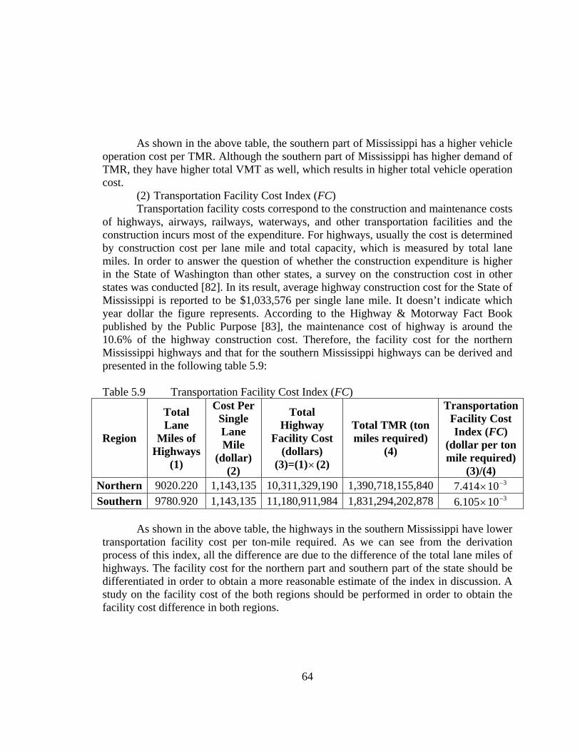
64

As shown in the above table, the southern part of Mississippi has a higher vehicle operation cost per TMR. Although the southern part of Mississippi has higher demand of TMR, they have higher total VMT as well, which results in higher total vehicle operation cost.

(2) Transportation Facility Cost Index (FC) Transportation facility costs correspond to the construction and maintenance costs

of highways, airways, railways, waterways, and other transportation facilities and the construction incurs most of the expenditure. For highways, usually the cost is determined by construction cost per lane mile and total capacity, which is measured by total lane miles. In order to answer the question of whether the construction expenditure is higher in the State of Washington than other states, a survey on the construction cost in other states was conducted [82]. In its result, average highway construction cost for the State of Mississippi is reported to be $1,033,576 per single lane mile. It doesn’t indicate which year dollar the figure represents. According to the Highway & Motorway Fact Book published by the Public Purpose [83], the maintenance cost of highway is around the 10.6% of the highway construction cost. Therefore, the facility cost for the northern Mississippi highways and that for the southern Mississippi highways can be derived and presented in the following table 5.9:

Table 5.9 Transportation Facility Cost Index (FC)

Region

Total Lane

Miles of Highways

(1)

Cost Per Single Lane Mile

(dollar) (2)

Total Highway

Facility Cost (dollars)

(3)=(1)× (2)

Total TMR (ton miles required)

(4)

Transportation Facility Cost Index (FC)

(dollar per ton mile required)

(3)/(4) Northern 9020.220 1,143,135 10,311,329,190 1,390,718,155,840 7.414 310−× Southern 9780.920 1,143,135 11,180,911,984 1,831,294,202,878 6.105 310−×

As shown in the above table, the highways in the southern Mississippi have lower

transportation facility cost per ton-mile required. As we can see from the derivation process of this index, all the difference are due to the difference of the total lane miles of highways. The facility cost for the northern part and southern part of the state should be differentiated in order to obtain a more reasonable estimate of the index in discussion. A study on the facility cost of the both regions should be performed in order to obtain the facility cost difference in both regions.

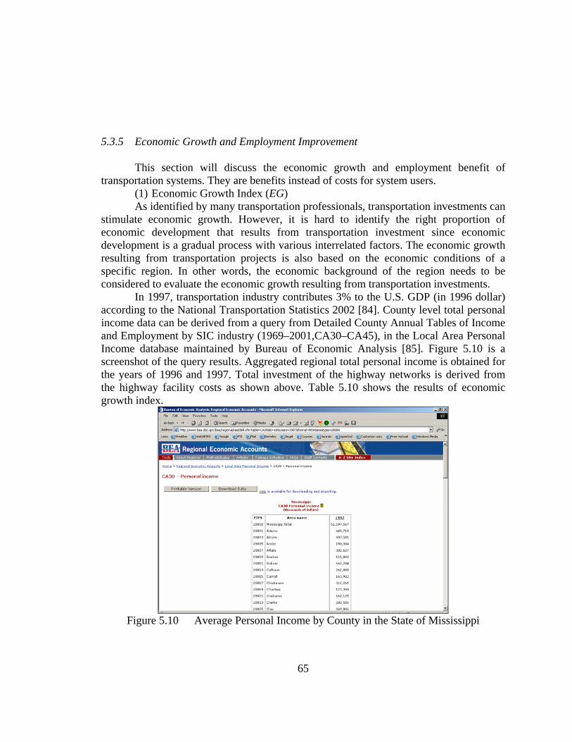
65

5.3.5 Economic Growth and Employment Improvement

This section will discuss the economic growth and employment benefit of transportation systems. They are benefits instead of costs for system users.

(1) Economic Growth Index (EG) As identified by many transportation professionals, transportation investments can

stimulate economic growth. However, it is hard to identify the right proportion of economic development that results from transportation investment since economic development is a gradual process with various interrelated factors. The economic growth resulting from transportation projects is also based on the economic conditions of a specific region. In other words, the economic background of the region needs to be considered to evaluate the economic growth resulting from transportation investments.

In 1997, transportation industry contributes 3% to the U.S. GDP (in 1996 dollar) according to the National Transportation Statistics 2002 [84]. County level total personal income data can be derived from a query from Detailed County Annual Tables of Income and Employment by SIC industry (1969–2001,CA30–CA45), in the Local Area Personal Income database maintained by Bureau of Economic Analysis [85]. Figure 5.10 is a screenshot of the query results. Aggregated regional total personal income is obtained for the years of 1996 and 1997. Total investment of the highway networks is derived from the highway facility costs as shown above. Table 5.10 shows the results of economic growth index.

Figure 5.10 Average Personal Income by County in the State of Mississippi

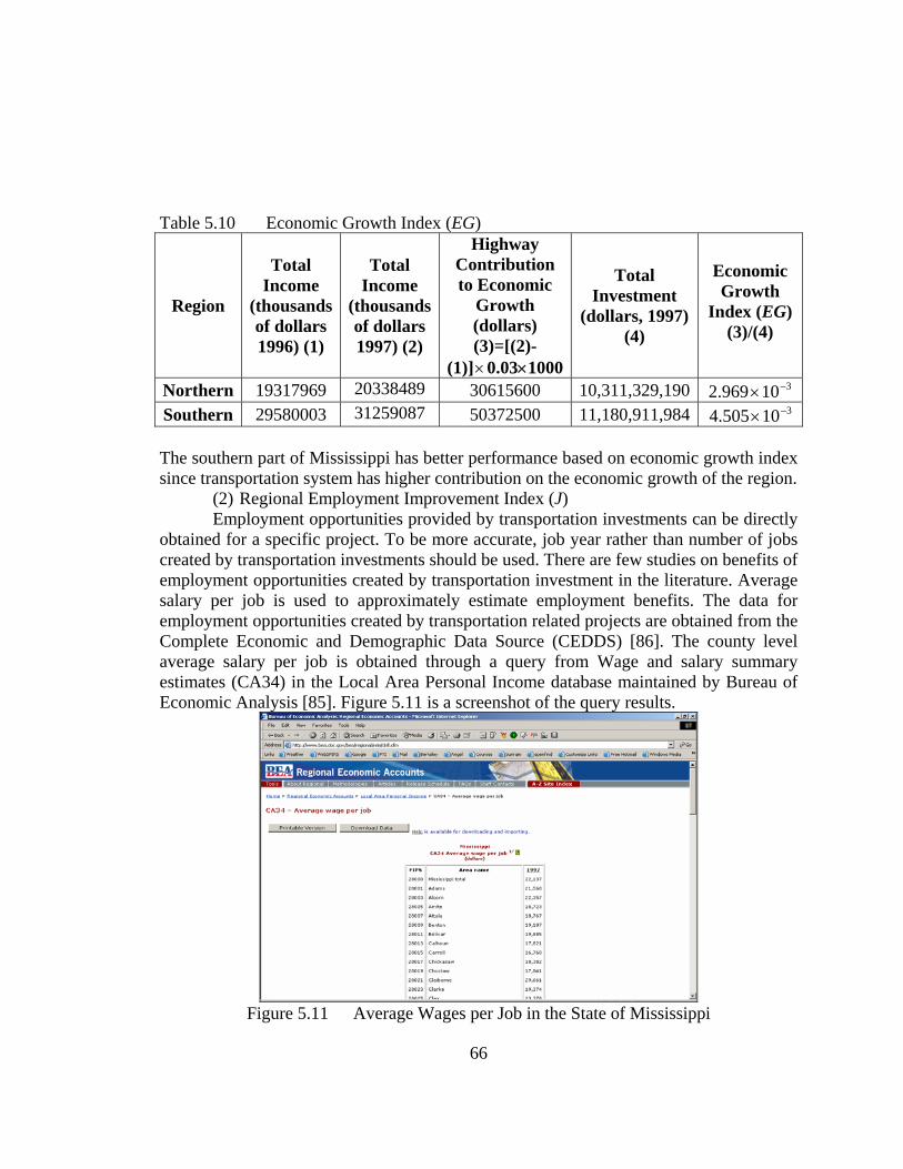
66

Table 5.10 Economic Growth Index (EG)

Region

Total Income

(thousands of dollars 1996) (1)

Total Income

(thousands of dollars 1997) (2)

Highway Contribution to Economic

Growth (dollars) (3)=[(2)-

(1)]×0.03×1000

Total Investment

(dollars, 1997) (4)

Economic Growth

Index (EG) (3)/(4)

Northern 19317969 20338489 30615600 10,311,329,190 310969.2 −×Southern 29580003 31259087 50372500 11,180,911,984 310505.4 −× The southern part of Mississippi has better performance based on economic growth index since transportation system has higher contribution on the economic growth of the region.

(2) Regional Employment Improvement Index (J) Employment opportunities provided by transportation investments can be directly

obtained for a specific project. To be more accurate, job year rather than number of jobs created by transportation investments should be used. There are few studies on benefits of employment opportunities created by transportation investment in the literature. Average salary per job is used to approximately estimate employment benefits. The data for employment opportunities created by transportation related projects are obtained from the Complete Economic and Demographic Data Source (CEDDS) [86]. The county level average salary per job is obtained through a query from Wage and salary summary estimates (CA34) in the Local Area Personal Income database maintained by Bureau of Economic Analysis [85]. Figure 5.11 is a screenshot of the query results.

Figure 5.11 Average Wages per Job in the State of Mississippi

67

A weighted average is obtained for the regional average salary per job. Table 5.10 shows the results of economic growth index.

Table 5.11 Regional Employment Improvement Index (J)

Region Employment (1)

Average Salary

(2)

Total Employment Improvement

(3)=(1)× (2)

Total Investment (4)

Regional Employment Improvement

Index (J) (3)/(4)

Northern 6,941 19,345.18 134,274,894 10,311,329,190 1.302 210−× Southern 14,093 20,412.18 287,668,853 11,180,911,984 2.572 210−×

Transportation investment in the southern Mississippi can yield a larger regional

employment improvement than those in the northern Mississippi as indicated by a higher Regional Employment Improvement Index.

5.3.6 Performance Indices Comparison in the State

As a summary, a complete table for all performance indexes for the northern Mississippi and southern Mississippi are listed in table 5.12. Table 5.12 Performance Measure Indices

Regions Performance Measures N. MS S. MS Mobility (M) 210103.2 −× 210999.1 −× 1. Mobility and Reliability

Reliability (Ru,R) N/A N/A Fatality (SF) 1.294 1110−× 1.038 1210−×

Injury Rate (SI) 2.948 1110−× 2.403 1110−× 2. Safety Property Damage (SP) N/A N/A

Transportation Pollutants (P)

1010059.2 −× 1010073.2 −×3. Environmental Impact Community Livability (L) N/A N/A Vehicle Operation Cost

(VC) 4.111 210−× 4.163 210−× 4. Long Term Cost Efficiency Transportation Facility

Cost (FC) 7.414 310−× 6.105 310−×

Economic Growth (EG) 310969.2 −× 310505.4 −× 5. Economic Growth and Employment Improvement Employment

Improvement (J) 1.302 210−× 2.572 210−×

Note: Please refer to the individual table for the unit of each index

68

A conceptual analysis of the highway network in the northern part of Mississippi and the southern part of Mississippi can be evaluated based on those performance measures. With some what-if scenarios analysis, decision makers may apply the performance measures to make a choice.

Note that some of the calculated index has very small value is due to the large TMR. With the units defined for each measure, the index is comparable for different sizes of transportation network which is one of the objectives of this study. As shown above from evaluation of each performance measures for the two regions. Some general conclusions can be obtained as the following:

o The southern MS network has better performance in terms of mobility in carrying within freight traffic

o The southern MS network has better performance in terms of safety due to the

lower value of fatality and injury rate. o The northern MS network has slightly better performance in terms of

environmental impact due to lower value of environment impact. o The northern MS network has lower vehicle operation cost and higher

transportation facility cost. In order to determine which region has better performance in terms of long term cost efficiency, a weight for these two measures has to be estimated appropriately.

o The southern MS network has better performance in terms of economic growth

and employment improvement due to the higher value for both measures.

Generally speaking, in order to give a final decision on which region has better overall performance, a model to incorporate all the related cost has to be built and weight for each performance measure has to be approximately estimated.

Based on discussion of data availability in the previous chapters and the practical experiences in the case study discussed above, a table on the data availability and sources is generated as in table 5.13.

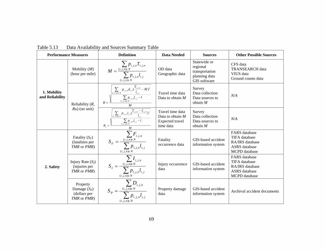
69

Table 5.13 Data Availability and Sources Summary Table Performance Measures Definition Data Needed Sources Other Possible Sources

Mobility (M) (hour per mile) ∑

∑

∈

∈=

Nnjijinji

Nnjinjinji

lp

TpM

),,(,,,

),,(,,,,

OD data Geographic data

Statewide or regional transportation planning data GIS software

CFS data TRANSEARCH data VIUS data Ground counts data

M

lp

Ml

Tdp

R Nnjijinji

Nnji ji

njijinji

1

)(

),,(,,,

),,(

2

,

,,,,,

−

−

=∑

∑

∈

∈

Travel time data Data to obtain M

Survey Data collection Data sources to obtain M

N/A 1. Mobility

and Reliability

Reliability (R, Ru) (no unit)

M

lpl

fTlp

R Nnjijinji

Nnji ji

njinjijinji

u

1

)(

),,(,,,

),,(

2

,

,,,,,,,

−

−

=∑

∑

∈

∈

Travel time data Data to obtain M Expected travel time data

Survey Data collection Data sources to obtain M

N/A

Fatality (SF) (fatalities per TMR or PMR) ∑

∑

∈

∈=

Nnjijinji

Nnjinji

F lp

FS

),,(,,,

),,(,,

Fatality occurrence data

GIS-based accident information system

FARS database TIFA database RA/IRS database ASRS database MCPD database

Injury Rate (SI) (injuries per

TMR or PMR) ∑∑

∈

∈=

Nnjijinji

Nnjinji

I lp

IS

),,(,,,

),,(,,

Injury occurrence data

GIS-based accident information system

FARS database TIFA database RA/IRS database ASRS database MCPD database

2. Safety

Property Damage (SP) (dollars per

TMR or PMR) ∑∑

∈

∈=

Nnjijinji

Nnjinji

P lp

DS

),,(,,,

),,(,,

Property damage data

GIS-based accident information system Archival accident documents

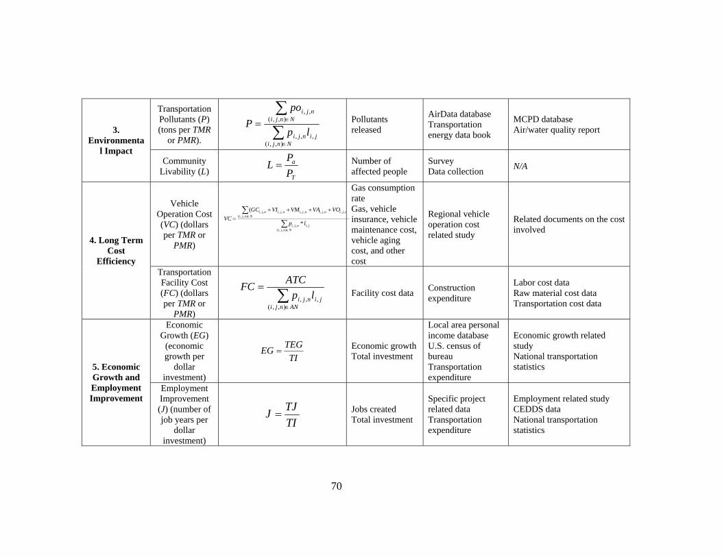
70

Transportation Pollutants (P) (tons per TMR

or PMR). ∑∑

∈

∈=

Nnjijinji

Nnjinji

lp

poP

),,(,,,

),,(,,

Pollutants released

AirData database Transportation energy data book

MCPD database Air/water quality report 3.

Environmental Impact

Community Livability (L)

T

a

PP

L = Number of affected people

Survey Data collection N/A

Vehicle Operation Cost (VC) (dollars per TMR or

PMR)

∑∑

∈

∈

++++=

Nnjijinji

Nnjinjinjinjinjinji

lp

VOVAVMVIGCVC

),,(,,,

),,(,,,,,,,,,,

*

(

Gas consumption rate Gas, vehicle insurance, vehicle maintenance cost, vehicle aging cost, and other cost

Regional vehicle operation cost related study

Related documents on the cost involved

4. Long Term Cost

Efficiency Transportation Facility Cost (FC) (dollars per TMR or

PMR)

∑∈

=

ANnjijinji lp

ATCFC

),,(,,,

Facility cost data Construction expenditure

Labor cost data Raw material cost data Transportation cost data

Economic Growth (EG)

(economic growth per

dollar investment)

TITEGEG = Economic growth

Total investment

Local area personal income database U.S. census of bureau Transportation expenditure

Economic growth related study National transportation statistics 5. Economic

Growth and Employment Improvement

Employment Improvement (J) (number of job years per

dollar investment)

TITJJ =

Jobs created Total investment

Specific project related data Transportation expenditure

Employment related study CEDDS data National transportation statistics

71

5.4 Discussion on Intermodal Aspect of the Case Study

In this study, only highway is used to evaluate the transportation performance of two Mississippi regions. Similarly, the data for other modes can be collected from various sources to obtain all of the proposed performance measures. The data collection processes for all other modes are not performed in this study in order to avoid unnecessary repetitions. There may exist better data sources than those used in the previous section, so more intensive research is necessary in the future before collecting data for other modes. Furthermore, TransCAD does not have networks for other modes’ networks except highways’ and does not have intermodal analysis capability as identified by Zhang, Bowden, and Allen [65]. In order to perform an intermodal transportation analysis, a similar simulation model to the Virtual Intermodal Transportation System (VITS) as discussed by Tan, Bowden, and Zhang [87] should be developed. With the VITS, the value for each of the proposed performance measure can be obtained by running simulation. Some what-if questions can be answered by the simulation model as well. For example, if the commodity flow increases due to the Latin American Trade, what is the performance of the transportation system in different regions might be and what kind of projects are the most cost effective in response to the changes of transportation needs.

5.5 Potential Applications This research result can be used to develop an essential tool to make correct and

scientific decisions. The transportation system performance measures can be applied in the following areas:

o Strategic policies and regulations development Transportation Demand Management (TDM) (also known as Mobility Management) is a technology to identify various strategies that can increase transportation system efficiency [78]. TDM helps to improve transportation systems to meet individual and community needs in the most efficient way, which often reduces total vehicle traffic [78]. With this proposed performance measure system, more TDM strategies can be implemented to improve transportation performance. At the same time, government agencies can use the set of performance measures and associated modeling methods for policy enactment.

o Performance based intermodal transportation planning in state level or regional level Intermodal transportation planning is under study by many state DOTs and MPOs. Performance goals can be set up based on the measures and drive performance based intermodal transportation planning. In different stages of development, the figures of these performance measures need to be predicted, estimated, and evaluated. and appropriate planning decision can be made based on the values of the measures. Performance measure system can influence the

72

overall interactive performance based transportation planning as do goals and objectives.

o Project prioritization Performance measure system can be used to evaluate performance of different projects under investigation. How to priority projects is one major concern of many researchers and DOT personnel. The priority can be obtained based on the life cycle cost and benefit ratio derived from the model. The performance measures developed in this research can be applied to evaluate transportation efficiency no matter what kind of modes are involved and what is the scale of the system. Potential improvements and alternatives can also be identified through the evaluation, as the suggestion proposed in the case study for Mississippi transportation.

o Industry decision making The performance measures can serve the industry as a guideline for decision making, especially mode choice decision-makings. With a systematic measure system, the questions related to transportation operation can be answered. The industry may focus on mobility and reliability, safety, and the direct cost measures.

73

CHAPTER VI AN INDUSTRIAL CASE

In this study, we investigate the finished vehicle distribution for Nissan, a major

automaker. Some of the performance measures defined in chapter IV can be verified by this industrial case.

6.1 Background Nissan has three assembly lines in the North America as well as plants in Japan and

Aquascalientes, Mexico. Two assembly lines are in the US: Smyrna, Tennessee, and Canton, Mississippi. Aguascalientes in Mexico has the other assembly line. The vehicles from Japan are shipped by over water to Los Angeles. Distribution Auto Service (DAS), a full subsidiary of Nissan, is responsible for the distribution of all Nissan vehicles. Their transportation problem is shipping finished vehicles from four origins to about twelve hundred dealers in the continental US. Two major modes are used by DAS to ship finished vehicles: truck or railway.

• Finished vehicles are shipped directly by trucks from the assembly line to the dealers. Figure 6.1 is the location of the dealers with the finished vehicles directly served by trucks from Canton, MS.

• The vehicles are shipped to some ramps by rail at first and then delivered by trucks from ramps to dealers. Figure 6.2 is an example of the ramps in northwest region.

Figure 6.1 Maps of the Dealers Directly Served by Trucks from Canton

Canton

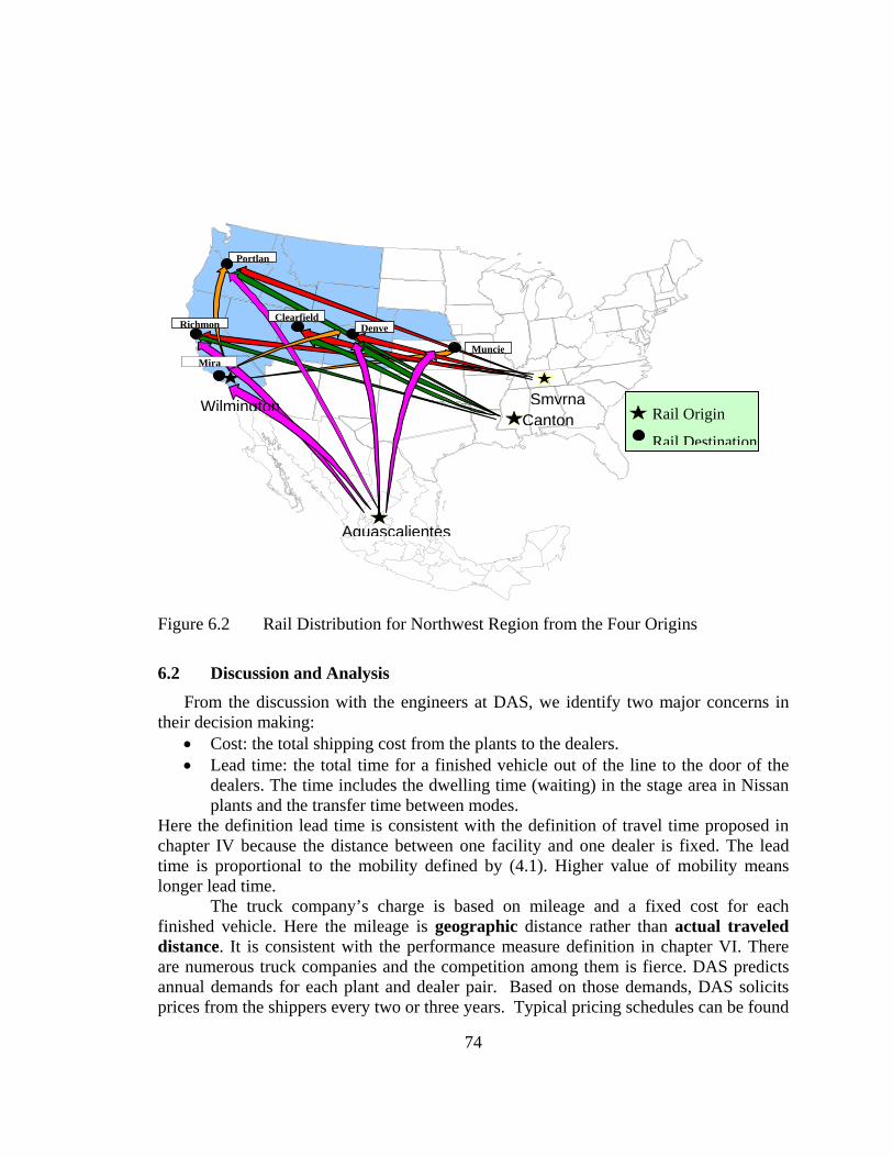
74

Figure 6.2 Rail Distribution for Northwest Region from the Four Origins

6.2 Discussion and Analysis From the discussion with the engineers at DAS, we identify two major concerns in

their decision making: • Cost: the total shipping cost from the plants to the dealers. • Lead time: the total time for a finished vehicle out of the line to the door of the

dealers. The time includes the dwelling time (waiting) in the stage area in Nissan plants and the transfer time between modes.

Here the definition lead time is consistent with the definition of travel time proposed in chapter IV because the distance between one facility and one dealer is fixed. The lead time is proportional to the mobility defined by (4.1). Higher value of mobility means longer lead time.

The truck company’s charge is based on mileage and a fixed cost for each finished vehicle. Here the mileage is geographic distance rather than actual traveled distance. It is consistent with the performance measure definition in chapter VI. There are numerous truck companies and the competition among them is fierce. DAS predicts annual demands for each plant and dealer pair. Based on those demands, DAS solicits prices from the shippers every two or three years. Typical pricing schedules can be found

Rail Origin

Rail Destination

Portlan

Muncie

SmyrnaCanton

Aguascalientes

DenveClearfield

Richmon

Mira

Wilmington

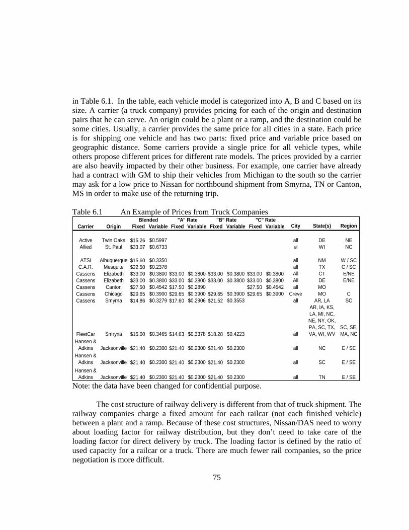
75

in Table 6.1. In the table, each vehicle model is categorized into A, B and C based on its size. A carrier (a truck company) provides pricing for each of the origin and destination pairs that he can serve. An origin could be a plant or a ramp, and the destination could be some cities. Usually, a carrier provides the same price for all cities in a state. Each price is for shipping one vehicle and has two parts: fixed price and variable price based on geographic distance. Some carriers provide a single price for all vehicle types, while others propose different prices for different rate models. The prices provided by a carrier are also heavily impacted by their other business. For example, one carrier have already had a contract with GM to ship their vehicles from Michigan to the south so the carrier may ask for a low price to Nissan for northbound shipment from Smyrna, TN or Canton, MS in order to make use of the returning trip.

Table 6.1 An Example of Prices from Truck Companies

Carrier Origin Fixed Variable Fixed Variable Fixed Variable Fixed Variable City State(s) Region

Active Twin Oaks $15.26 $0.5997 all DE NEAllied St. Paul $33.07 $0.6733 all WI NC

ATSI Albuquerque $15.60 $0.3350 all NM W / SCC.A.R. Mesquite $22.50 $0.2378 all TX C / SC

Cassens Elizabeth $33.00 $0.3800 $33.00 $0.3800 $33.00 $0.3800 $33.00 $0.3800 All CT E/NECassens Elizabeth $33.00 $0.3800 $33.00 $0.3800 $33.00 $0.3800 $33.00 $0.3800 All DE E/NECassens Canton $27.50 $0.4542 $17.50 $0.2890 $27.50 $0.4542 all MOCassens Chicago $29.65 $0.3900 $29.65 $0.3900 $29.65 $0.3900 $29.65 $0.3900 Creve MO CCassens Smyrna $14.86 $0.3279 $17.60 $0.2906 $21.52 $0.3553 all AR, LA SC

FleetCar Smryna $15.00 $0.3465 $14.63 $0.3378 $18.28 $0.4223 all

AR, IA, KS, LA, MI, NC, NE, NY, OK, PA, SC, TX, VA, WI, WV

SC, SE, MA, NC

Hansen & Adkins Jacksonville $21.40 $0.2300 $21.40 $0.2300 $21.40 $0.2300 all NC E / SE

Hansen & Adkins Jacksonville $21.40 $0.2300 $21.40 $0.2300 $21.40 $0.2300 all SC E / SE

Hansen & Adkins Jacksonville $21.40 $0.2300 $21.40 $0.2300 $21.40 $0.2300 all TN E / SE

Blended "A" Rate "B" Rate "C" Rate

Note: the data have been changed for confidential purpose.

The cost structure of railway delivery is different from that of truck shipment. The railway companies charge a fixed amount for each railcar (not each finished vehicle) between a plant and a ramp. Because of these cost structures, Nissan/DAS need to worry about loading factor for railway distribution, but they don’t need to take care of the loading factor for direct delivery by truck. The loading factor is defined by the ratio of used capacity for a railcar or a truck. There are much fewer rail companies, so the price negotiation is more difficult.

76

In general, railway delivery has longer lead time than truck delivery, especially for the ramps with low volume demands. Since railway service is charged based on the number of used railcars rather than the number of finished vehicles, Nissan/DAS may have to delay the delivery of some finished vehicles and temporarily store them in the stage area of the plants waiting for the future vehicles for the same ramp to increase the loading factor of railcars. A railcar may stop in some ramps because of consolidation by railway companies.

Nissan/DAS needs to make the following decisions for each pair of dealer and origin:

• What kind of mode or modes should be selected? • If rail is selected, where is the ramp? • Who are the transportation service providers?

Since cost is the major concern, the decisions for most dealers are easy. In general, direct delivery by trucks is used for the dealers who are close to the origin, and the closest ramp is chosen for a dealer far away from the origin. However, some dealers are around the borders of direct shipment areas or between multiple ramps, and then some careful analysis is necessary to find out the optimal solution. We analyze the shipment from Canton, MS and identify some improvement opportunities. The annual cost savings is about $77,000 (please refer to the attached letter from DAS) just for the Canton plant. To reduce the lead time, some dealers are not served by the cheapest way. The volume of some ramps is too small to consider because of long lead time. They are usually removed and the nearby dealers are served by trucks through other close ramps. Long lead time means not only long waiting time for dealers but also high inventory carrying cost in the stage area of the plants. From this case, we learn than the major concerns an industrial company are costs and travel time, which are covered by Vehicle Operation Cost (VC) and mobility (M) in our proposed performance measures. Their secondary interests are environmental impact and economic growth, which are the interests of governments and the public. Safety issues are usually taken care of by transportation service providers. This case is consistent with our initial analysis on intermodal transportation users and their needs.

6.3 Redistribution Problem

So far, direct delivery by truck and combined delivery of rail-truck have been discussed. For the dealers in the west and plants in Canton and Smyrna, railway is usually used to take advantage of its low costs. Rail is used to transport the vehicles from Smyrna or Canton to Memphis and then to the ramp. It may take a long time for some vehicles to wait in Smyrna or Canton to fill a railcar. A possible solution is redistribution of truck-rail-truck combinations. Trucks are used to transport vehicles from Smyrna and Canton to Memphis, and then the vehicles are consolidated to fill a railcar and shipped by rail to the ramp. Figure 6.3 is used to illustrate the redistribution problem.

77

Figure 6.3 Redistribution Illustration

The following example is given to show the advantages of redistribution. Assume a railcar can hold 21 vehicles. If there are 10 cars in Canton for one ramp, it may take another 7 days to have another 11 cars in Canton to this ramp. If there are another 11 cars in Smyrna for the same ramp, it may take another 5 days to have another 10 cars in Smyrna to this ramp. With redistribution, all these 21 available vehicles are transported by trucks from Canton and Smyrna and then loaded on a railcar. Therefore, the waiting time is significantly reduced.

Obviously, redistribution can decrease the lead time for the vehicles to low volume ramps. However, there are also some disadvantages:

• More cost for truck transportation from Smyrna or Canton to Memphis, • Some additional loading costs in Memphis, • Some additional complexity for operation.

Therefore, redistribution should only be implemented when it is necessary. Since different models have different lengths and their loading may influence the loading factor of a railcar. Loading factor should be considered by DAS rather than railway companies because of the cost structure. When and how to do redistribution is a hard question, so some sophisticated tools are necessary for this intermodal transportation decisions. We developed a mathematical programming optimization model to deal with the redistribution.

Canton

Smyrna

Memphis

Rail

Rail

Rail to the ramp

Canton

Smyrna

Memphis

Truck

Truck

Rail to the ramp

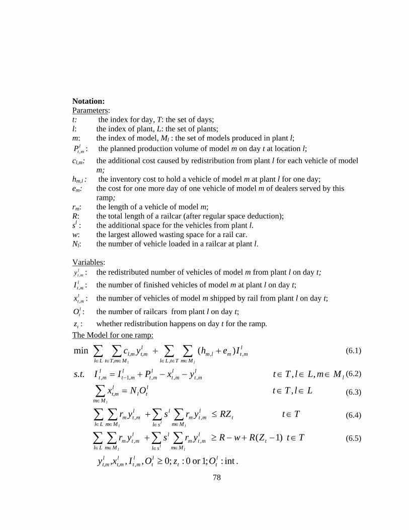
78

.int:;1or 0:;0,,

)1(

,

,,

)( min

,

,,

,,

,,,,1,

,,,

ltt

lt

lmt

lt,m

lt,m

tsl Mm

lmtm

l

Ll Mm

lmtm

tsl Mm

lmtm

l

Ll Mm

lmtm

ltl

Mm

lt,m

ll

mtl

mtlmt

lmt

lmt

TtLl Mm

lmtmlm

Ll MT,mt

lt,ml,m

OzOI,x y

TtZRwR yrs yr

Tt RZ yrs yr

LlT t ONx

MmLlT t yxPIs.t. I

Ieh yc

lll

lll

l

ll

≥

∈−+−≥+

∈≤+

∈∈=

∈∈∈−−+=

++

∑ ∑∑ ∑

∑ ∑∑ ∑

∑

∑ ∑∑ ∑

∈ ∈∈ ∈

∈ ∈∈ ∈

∈

−

∈∈ ∈∈ ∈∈

Notation: Parameters: t: the index for day, T: the set of days; l: the index of plant, L: the set of plants; m: the index of model, Ml : the set of models produced in plant l;

lmtP , : the planned production volume of model m on day t at location l;

cl,m: the additional cost caused by redistribution from plant l for each vehicle of model m;

hm,l : the inventory cost to hold a vehicle of model m at plant l for one day; em: the cost for one more day of one vehicle of model m of dealers served by this

ramp; rm: the length of a vehicle of model m; R: the total length of a railcar (after regular space deduction); sl : the additional space for the vehicles from plant l. w: the largest allowed wasting space for a rail car. Nl: the number of vehicle loaded in a railcar at plant l. Variables:

lmty , : the redistributed number of vehicles of model m from plant l on day t;

lmtI , : the number of finished vehicles of model m at plant l on day t;

lmtx , : the number of vehicles of model m shipped by rail from plant l on day t; ltO : the number of railcars from plant l on day t;

tz : whether redistribution happens on day t for the ramp. The Model for one ramp:

(6.1)

(6.2)

(6.3)

(6.4)

(6.5)

79

The model is explained by the following: 1. Objective function (6.1): the objective is to minimize all costs: additional

redistribution cost, vehicle holding cost in plants, and the penalty of one more day of lead time.

2. Inventory balanced constrain (6.2): The number of vehicles of model m at plant l at the end of day t

= The number of vehicles of model m at plant l at the end of day t-1 + the planned production of vehicles of model m at plant l on day t

- the number of vehicles of model m shipped by the regular railcars - the number of vehicles of model m shipped by the redistribution trucks.

3. Rail delivery constraint (6.3): the number of vehicles shipped by the regular rail at plant l should fill integer number of railcars.

4. Rail delivery constraint (6.4): when any vehicles are shipped by trucks, redistribution happens and the total length of the redistributed vehicles cannot exceed the available length of a railcar.

5. Railcar loading factor requirement constraint (6.4): when redistribution happens, the total length of the redistributed vehicles should exceed a required length.

In this math model, we assume the lengths of the models that are produced in the same plant are close to each other. This math model uses rolling horizon method. It is solved for the next d days and only today’s plan is implemented. Tomorrow, the model is solved again for d days with updated information.

This model captures the situation of truck-rail-truck intermodal transportation. The key point of this model is coordination: the coordination among plants and the coordination between two transportation modes. If there are not enough vehicles to fill a railcar in the redistribution center, no redistribution should be done. The objective of the model captures the two major concerns of an industrial company: cost and lead time. This model can help to reach the trade-off between these two measures.

This model is verified by DAS, but it has not been fully implemented because some advanced optimization software is required to solve this sophisticated model and DAS doesn’t have this kind of software, which is expensive. We may develop some heuristics for DAS to obtain some good solutions rather than the optimal solution.

80

CHAPTER VII CONCLUSIONS AND FUTURE WORK

The objective of this report is to establish a systematic and user-oriented performance measurement system for intermodal transportation and to use case studies to demonstrate and verify the proposed performance measure system. Based on an intensive literature review on transportation performance measures in chapter II of this report, a system level measurement system for any transportation system with different modes and sizes is identified to promote intermodalism in the U.S. Transportation characteristics are analyzed in chapter III in order to help generalize system performance measures for intermodal transportation. After identifying transportation users (interest parties) and their needs in section 4.1 with the U.S. transportation goals in section 4.2, intermodal transportation performance measures are defined on the system level, which are significantly different from those in practice and the literature. The proposed performance measures are discussed in detail in section 4.5 in this report. Five main categories are identified to measure intermodal transportation: mobility and reliability for travel time, safety measures, environmental impact, long term transportation cost efficiency, and economic impact. The developed measure system is user-oriented, scalable, and systematic for intermodal transportation as shown by the definition of those measures (section 4.5) and the case study following (chapter 5).

The performance measures are carefully distinguished from factors. Performance measures are used to evaluate a design or an existing system and to see how well it can satisfy customers. Factors, like capacity, facility condition, accessibility, and others, which are usually defined as measures in the literature, are essentially controllable parameters influencing measures. Project prioritization and the decisions regarding project funding should be based on the values of performance measures rather than the factors.

The proposed measure system is the first one targeted at intermodal transportation and applicable for all kinds of modes as their definitions are not mode specific [88]. Under each category, there are several system-level measures, which are critical to evaluate a transportation system. In other words, they are main costs (benefits) that should be considered during decision making. In practice, different users for different purposes may choose a subset of the proposed performance measures to meet their needs.

A case study is performed for the State of Mississippi highway network as discussed in chapter V. The case study demonstrates how to collect data for those performance measures and suggests improvements. Though some data are available for other modes of transportation system, it is hard to get all data, especially integrated data, for intermodal transportation. This will promote the data-collection effort for intermodal transportation systems.

Another case study based on Nissan/DAS intermodal network for finished vehicle distribution is performed in chapter VI to help industries improve intermodal efficiency.

81

A mode choice analysis helps the company to have $77,000 in annual savings. The case study also verifies the proposed performance measures, especially for the usage of geographic distance as mileage and the total travel time for mobility. A math model is developed to promote the intermodalism of truck-rail-truck combinations for distribution in order to reach the trade-off between costs and lead time.

Since our intermodal transportation performance measure system is significantly different from the existing measures, obtaining required data is a big concern. Although there is some preliminary discussion in section 4.6 of the report, some future research on data acquisition is still necessary. In this report, only system level performance measures are studied. The factors influencing these measures should also be identified in a future study and the results can help transportation designers and decision makers to take effective actions to improve transportation system efficiency. Applying the measures in practice, demonstrating their feasibility based on case studies, and implementing the measures in decision making tools also require further efforts.

82

REFERENCES [1] National Transportation Library. The Intermodal Transportation Efficiency Act of

1991 (ISTEA). Originally accessed at http://ntl.bts.gov/DOCS/ste.html, February 19, 2003.

[2] Federal Highway Administration website. TEA-21 Moving Americans into 21st century. Originally accessed at http://www.fhwa.dot.gov/tea21/, February 19, 2003.

[3] U.S. Department of Transportation. Originally accessed at http://www.dot.gov/PerfPlan2004/intro_strategic.html, February 15, 2003.

[4] Federal Highway Administration (FHWA) 1998 National Strategic Plan. Originally accessed at http://www.fhwa.dot.gov/policy/fhplan.html, February 15,

2003 [5] Freight Program Overview, FHWA Office of Operations. Originally accessed at

http://ops.fhwa.dot.gov/freight/overview/overview.htm, Feburary 19, 2003

[6] “Status of Achieving Key Outcomes and Addressing Major Management Challenges”, U.S. Department of Transportation, 2001

[7] “Institutional Barriers to Intermodal Transportation Policies and Planning in Metropolitan area”, Transportation Research Board, National Research Council, 1996

[8] G.S. Rutherford, “Multimodal Evaluation of Passenger Transportation,” NCHRP, Synthesis of Highway Practice 201, Transportation Research Board, National Research Council.

[9] P. Bickel, S Schmid., W. Krewitt, and R. Friedrich “External Costs of Transport in Externe” Publishable Report, IER, Germany, 1997

[10] B. Blanchard and F. Wolter, “System Engineering and Analysis: 3rd edition” Prentice-Hall, 1998

[11] Mobility and Economic Growth, U.S. DOT Performance Plan for 2004. Originally accessed at http://www.dot.gov/PerfPlan2004/mobiity.html, February 19, 2003.

[12] Highway Safety, U.S. DOT Performance Plan for 2004. Originally accessed at http://www.dot.gov/PerfPlan2004/safety_highway.html, February 19, 2003.

83

[13] Safety, U.S. DOT Performance Plan for 2004. Originally accessed at http://www.dot.gov/PerfPlan2004/safety, February 19, 2003.

[14] Human and Natural Environment, U.S. DOT Performance Plan f0r 2004. Originally accessed at http://www.dot.gov/PerfPlan2004/humanperf.html, February 19, 2003.

[15] Hagler Bailly Services, Inc. “Measuring Improvements in the Movement of Highway and Intermodal Freight”, Final Report Prepared for Federal Highway Administration, 2001.

[16] BRW, Inc, “CDOT Travel Demand Improvement Projects: Improvements to Mobility Performance Measure Calculations”. Report Prepared for Colorado Department of Transportation, 2000.

[17] M.D. Meyer, “Measuring That Which Cannot Be Measured—At Least According to Conventional Wisdom”. Conference Proceedings 26 of Performance Measures to Improve Transportation Systems and Agency Operations, 2001.

[18] R.L. Bertini, M. Leal, and D.J. Lovell, “Generating Performance Measures from Portland’s Archived Advanced Traffic Management System Data”. Transportation Research Board, 2002.

[19] T. Shaw, “ITS Program Performance Measures: ITS Corridor Master Plans for Florida’s Principal FIHS Limited-Access Corridors”. Report Prepared for Florida Department of Transportation, 2002.

[20] Albany, New York, Case Study and the Transportation Improvement Program, Report of a Conference, Conference Proceedings 26, “Performance Measures to Improve Transportation Systems and Agency Operations”. Transportation Research Board, The National Academies, 2001.

[21] R.L. Bertini and A. El-Geneidy, “Using Archived Data to Generate Transit Performance Measures”. Transportation Research Board, Washington D.C. 2003.

[22] Metropolitan Transportation Commission. “Performance measures report for the 2001 regional transportation plan for the San Francisco Bay Area. 2001”. 2001.

[23] E. Dumbaugh and M.D. Meyer, “Exploring the Relationship between Agency Performance Measues and Operations Investments in a Metropolitan Area”. Transportation Research Board, 2003.

84

[24] R. Czerniak, S. Gasier and D. Gerard, “The Use of Intermodal Performance Measures by State Departments of Transportation”. Prepared for U.S. DOT, 1996.

[25] Planning and Intermodal Mobility, BI 2001-2003 Research Program, Washington Department of Transportation. Originally accessed at http://www.wsdot.wa.gov/ppsc/research/BI0103/Mob0103.html, February 19, 2003.

[26] Report of a Conference, Conference Proceedings 26, “Performance Measures to Improve Transportation Systems and Agency Operations”. Transportation Research Board, The National Academies, 2001.

[27] U.S. Department of Transportation, “Combined Performance Plan and Report”. Performance Report for the Year 2001 and Performance Plan for the Year 2003, March, 2002

[28] Ministry of Environment and Energy and National Environmental Research Institute. “Indicators and Performance Measures for Transportation, Environment, and Sustainability in North America”. Report from a German Marshall Fund Fellowship 2000.

[29] Federal Highway Administration (FHWA) Air Quality Performance Measures Fiscal Year (FY) 2002. Originally accessed at http://www.fhwa.dot.gov/environment/perform/aqrpt02.htm, February 19, 2003.

[30] Hickling Lewis Brod, Inc. “Workshop on Productivity Performance Indicators: Report of Proceedings”. Sponsored by U.S. DOT. May 1998.

[31] Department of Transportation, the State of Florida. “Report to Statewide Model Task Force on Freight Modeling and Forecasting Techniques”. February 1998.

[32] California Department of Transportation (Caltrans). “1998 California Transportation Plan: Statewide Goods Movement Strategy”. August 1998.

[33] Act 51 Transportation Funding Study Committee. “Act 51 White Paper – State Trunklines: Performance Measures”. 1999.

[34] “Economic Performance Measures”. A Technical Report from ‘The I-69 Evansville-to-Indianapolis Study, 2000.

[35] East-West Gateway Coordinating Council (St. Louis Region MPO). “Goods Movement Issue Paper”. August 1998.

85

[36] B. Thompson, “Performance Evaluation of Florida’s Public Transit Systems”. Poster Session in Conference Proceedings 26 of Performance Measures to Improve Transportation Systems and Agency Operations, 2001.

[37] U.S. Department of Transportation, Federal Highway Administration (FHWA), “Examination of Transportation Industry Productivity Measures”. Conference Summary Report, 1993.

[38] W.B. Jones, C.R. Cassady, and R.Bowden. Developing a Standard Definition of Intermodal Transportation. Intermodal Transportation: Selected Essays, National Center for Intermodal Transportation, 2001.

[39] FHWA Office of Operations. Originally accessed at http://ops.fhwa.dot.gov/Travel/Deployment_Task_Force/perf_measures.htm, November 22, 2002.

[40] Conference Summary Report, “Performance Measures for California Transportation System Users and Investors”. UCLA Extension Public Policy Program, 1997

[41] U.S. Department of Transportation, Federal Highway Administration, and Federal Transit Administration. “1997 Status of the Nation’s Surface Transportation System: Condition and Performance”. Report to Congress. 1998.

[42] National Center for Intermodal Transportation. “A New Agenda for America: in the Aftermath of 11 September 2001”. November 2001.

[43] U.S. Department of Transportation. “An Assessment of the U.S. Marine Transportation System”. A Report to Congress, September 1999.

[44] The Minnesota department of Transportation. “Quantitative Research Regarding Performance Measures for Intermodal Freight Transportation.”. October 1995.

[45] Oregon’s Intermodal Management System, Summary Report. Originally accessed at http://www.odot.state.or.us/intermodal-freight/Reports/Ims-summ.PDF , March, 2003.

[46] Recommendations of the Minnesota Freight Committee, Freight Performance Measures: A Yardstick for Minnesota’s Transportation System. Measurement and Evaluation Section and Office of Freight, Rail and Waterways, Minnesota Department of Transportation .1999.

86

[47] Capital Improvement Program. Originally accessed at http://www.deldot.net/static/cip01-06/execsumm/prioritizing.html Nov.22,2002

[48] Ohio Department of Transportation. Transportation Review Advisory Council Policies for Selecting Major New Capacity Projects. February 2001. Originally accessed at http://www.dot.state.oh.us/trac/book2002.pdf, Nov. 23, 2001

[49] Florida Mobility Performance Measures Program. Originally accessed at http://www11.myflorida.com/planning/statistics/mobilitymeasures/mmpresentation.pdf, March 2003.

[50] Railroad Performance Measures Website. Originally accessed at http://www.railroadpm.org/welcome_rpm.cfm, January 10 2003.

[51] Burlington Northern Santa Fe Railway (BNSF).Originally accessed at http://www.railroadpm.org/bnsf/definition_bnsf.cfm, February 2003.

[52] CSX Corporation. Originally accessed at http://www.csxt.com, February 2003,

[53] Norfolk Southern. Originally accessed at http://www.nscorp.com/stb, February 2003.

[54] Kansas City Southern. Originally accessed at http://www.kcsi.com/customers.html, February 2003.

[55] Union Pacific. Originally accessed at http://www.uprr.com/, February 2003.

[56] Aviation Safety, FY 2004 Performance Plan. U.S. Department of Transportation. Originally accessed at http://www.dot.gov/PerfPlan2004/safety_aviation.html, April 2003.

[57] Booz. Allen & Hamilton Inc. “Transportation System Performance Measures Aviation: Technical Memorandum”. Transportation System Information Program, California Department of Transportation. November 2001.

[58] Donald J. Guffey, “Capacity Enhancement Developments and System Performance Measures”. Office of System Capacity, Federal Aviation Administration. May 1998.

[59] National Center for Intermodal Transportation. Originally accessed at http://www.ie.msstate.edu/ncit/INTRODUCTION.html, January 2003.

87

[60] Beimborn, A., Eduard “A Transportation Modeling Primer”. Center for Urban Transportation, University of Wisconsin-Milwaukee, May 1995.

[61] S. Pickell and L. Neumann, Cambridge Systematics, Inc. “Resource Paper: Use of Performance Measures in Transportation Decision Making”. 2000.

[62] D. L. Hoyert and S. L. Murphy, “Deaths: Final Data for 1999”. National Vital Statistics Report, Vol. 49, No. 8, 2001.

[63] “Urban Transportation Fact Book”. The Public Purpose, Wendell Cox Consultancy at www.publicpurpose.com, May. 2003.

[64] J. A. Lindley; "Urban Freeway Congestion: Quantification of the Problem and Effectiveness of Potential Solutions". ITE Journal; January 1987.

[65] Y. Zhang, R. O. Bowden, A. J. Allen, “Intermodal Transportation Planning Using Commodity Flow Data”. Final report submitted to National Center for Intermodal Transportation and Mississippi Department of Transportation, June 2003.

[66] Transportation Energy Data Book. Edition 22. Oak Ridge National Laboratory, 2002. 17 TEDB ORNL.

[67] U.S. Bureau of Census. Originally accessed at http://www.census.gov/main/www/cen2000.html, March 2003.

[68] California PeMS (Performance Measure System). originally accessed at http://transacct.eecs.berkeley.edu, March. 10, 2003.

[69] TransCAD-Transportation GIS software. Caliper Corporation, Newton, Massachusetts, 2001.

[70] Fatality Analysis Reporting System (FARS). Originally accessed at http://www-fars.nhtsa.dot.gov/queryReport.cfm, July, 2003.

[71] Truck Involved in Fatal Accidents Database. Originally accessed at http//www.transtats.bts.gov/Tables.asp?DB_ID=415&DB_Name=Trucks%20Involved%20in%20Fatal%20Accidents%20%28TIFA%29&DB_Short_Name=TIFA , July, 2003

[72] Railroad Accident/Incident Reporting System. Originally accessed at http://itdb.bts.gov/Tables.asp?DB_ID=195&DB_Name=Railroad%20Accident/Incident%20Reporting%20System&DB_Short_Name=Railroad%20Accidents, July, 2003

88

[73] Aviation Safety Reporting System (ASRS). Originally accessed at http://asrs.arc.nasa.gov/main.htm, July 2003.

[74] Marine Casualty and Pollution Database. Originally accessed at http://itdb.bts.gov/Tables.asp?DB_ID=610&DB_Name=Marine%20Casualty%20And%20Pollution%20Database&DB_Short_Name=Marine%20Casualty/Pollution, July 2003

[75] U.S. Emissions Inventory 1999. Originally accessed at http://yosemite.epa.gov/oar/globalwarming.nsf/content/ResourceCenterPublicationsGHGEmissionsUSEmissionsInventory1999.html, August 2003.

[76] Air Pollution Data (AirData). Originally accessed at http://www.epa.gov/air/data/geosel.html, August 2003.

[77] MOBILE 6 Vehicle Emission Modeling Software. Originally accessed at http://www.epa.gov/otaq/m6.htm, August 2003.

[78] Victoria Transport Benefit Analysis (VTPI), TDM Encyclopedia. Originally accessed at www.vtpi.org/tdm/tdm82.htm, January 2003.

[79] The Office of Transportation Technologies. Originally accessed at www.ott.dot.gov/benefits.html, March 2003.

[80] International Energy Agency. Originally accessed at http://www.iea.org on March 2003.

[81] CUTEP Guide to Transportation Benefit-Cost Analysis, TOPIC: Valuation of Vehicle Operating Cost. Originally accessed at http://ceenve.calpoly.edu/sullivan/cutep/cutep_topic_B1c.htm, August 2003.

[82] Highway Construction Cost Comparison Survey. Originally accessed at http://www.wsdot.wa.gov/biz/construction/I-C_Const_Cost.pdf, August 2003.

[83] Highway & Motorway Fact Book. Originally accessed at http://www.publicpurpose.com/hwy-fy$.htm, August 2003.

[84] National Transportation Statistics 2002. Originally accessed at http://www.bts.gov/publications/national_transportation_statistics/2002/index.html, August 2003.

[85] Regional Economic Accounts, Bureau of Economic Analysis. Originally accessed at http://www.bea.doc.gov/bea/regional/reis/default.cfm, August 2003.

89

[86] Woods and Pool Economics. “The Complete Economic and Demographic Data Sources (CEDDS)”. Washington D.C. 2001.

[87] A. Tan, R. Bowden, and Y. Zhang, “Virtual Simulation of Statewide Intermodal Freight Traffic”. Transportation Research Board, January 2004.

[88] H. Wang, M. Jin, and N. Rana, “A New Performance Measure System for Intermodal Transportation”. Transportation Research Board, January 2004.

90

Appendix Support Letter from DAS