Tetsuo Sasao and Andre B. FletcherIntroduction to VLBI SystemsChapter 3Lecture Notes for KVN StudentsPartly Based on Ajou University Lecture NotesIssued July 14, 2005revised September 25, 2005revised October 28, 2005revised November 11, 2005(to be further edited)

Radio Interferometry

Contents

1 Fundamentals of Radio Interferometry 41.1 Two Explanations of VLBI . . . . . . . . . . . . . . . . . . . . 4

1.1.1 VLBI System . . . . . . . . . . . . . . . . . . . . . . . 41.1.2 “Geodetic” Explanation — Noise Approach . . . . . . 51.1.3 “Astrophysical” Explanation — Monochromatic Wave

Approach . . . . . . . . . . . . . . . . . . . . . . . . . 61.1.4 Superposition of Monochromatic Waves . . . . . . . . . 71.1.5 Fringe Pattern Appears within an Envelope . . . . . . 91.1.6 Peak of the Envelope . . . . . . . . . . . . . . . . . . . 91.1.7 Fringe Pattern Enclosed by the Envelope . . . . . . . . 10

1.2 Elements of Stationary Random Processes . . . . . . . . . . . 121.2.1 Basic Concepts . . . . . . . . . . . . . . . . . . . . . . 131.2.2 Random Processes in Linear Systems . . . . . . . . . . 261.2.3 Stationary Random Processes . . . . . . . . . . . . . . 281.2.4 Ergodicity . . . . . . . . . . . . . . . . . . . . . . . . 301.2.5 Stationary Random Processes in Linear Systems . . . . 331.2.6 Spectra of Stationary Random Processes . . . . . . . . 351.2.7 Spectra of Outputs of Linear Systems . . . . . . . . . . 411.2.8 Two Designs of Spectrometers . . . . . . . . . . . . . . 431.2.9 Fourier Transforms of Stationary Random Processes . . 45

1

1.3 The White Fringe . . . . . . . . . . . . . . . . . . . . . . . . . 491.3.1 A Simple Interferometer . . . . . . . . . . . . . . . . . 491.3.2 Received Voltages as Stationary Random Processes . . 501.3.3 Cross–Correlation of Received Voltages . . . . . . . . . 511.3.4 Fringe Pattern Enclosed by Bandwidth Pattern . . . . 551.3.5 Amplitude and Phase Spectra of the Correlated Signals 581.3.6 Coherence Interval in the Sky . . . . . . . . . . . . . . 591.3.7 Fringe Spacing in the Sky . . . . . . . . . . . . . . . . 60

2 A Realistic Radio Interferometer 612.1 Source Structure, Visibility and Intensity . . . . . . . . . . . . 63

2.1.1 Source Coherence Function . . . . . . . . . . . . . . . . 632.1.2 Power of Electric Field Incident from a Certain Direction 652.1.3 Poynting Flux . . . . . . . . . . . . . . . . . . . . . . . 662.1.4 Electric Field and Radio Source Intensity — Electro-

magnetics and Astronomy . . . . . . . . . . . . . . . . 692.1.5 Field of View of a Radio Telescope . . . . . . . . . . . 702.1.6 Power Pattern of a Receiving Antenna . . . . . . . . . 722.1.7 New Dimensions of Voltage and Electric Field . . . . . 742.1.8 How Does A Radio Interferometer View the Universe? 752.1.9 Complex Visibility . . . . . . . . . . . . . . . . . . . . 79

2.2 Frequency Conversion in Radio Interferometers . . . . . . . . 802.2.1 Response of RF Filters . . . . . . . . . . . . . . . . . . 812.2.2 Fourier Transform of IF Voltage Signal . . . . . . . . . 832.2.3 Cross–Correlation of Fourier Transforms of IF Signals . 842.2.4 Roles of Low–Pass Filters . . . . . . . . . . . . . . . . 862.2.5 Relationship between RF Spectrum and IF Spectrum . 88

2.3 Delay Tracking and Fringe Stopping . . . . . . . . . . . . . . . 912.3.1 General Form of Cross–Power Spectrum of IF Signals . 912.3.2 “Expected Correlation” of IF Signals . . . . . . . . . . 952.3.3 Radio Source Tracking by an Interferometer . . . . . . 982.3.4 Requirements to the Delay Tracking and Fringe Stopping1002.3.5 Insertion of Instrumental Delay at IF Band . . . . . . . 1042.3.6 Separation of Delay Tracking and Fringe Stopping Due

to Frequency Conversion . . . . . . . . . . . . . . . . . 1062.3.7 Actual Implementations of Delay Tracking . . . . . . . 1082.3.8 Actual Implementations of Fringe Stopping . . . . . . . 109

2.4 Correlator Outputs . . . . . . . . . . . . . . . . . . . . . . . . 1132.4.1 Multiplier and Integrator . . . . . . . . . . . . . . . . . 1132.4.2 Single Sideband (USB or LSB) Reception . . . . . . . . 1152.4.3 Correlator Outputs in Single Sideband Reception . . . 117

2

2.4.4 Fringe Amplitude and Fringe Phase . . . . . . . . . . . 1192.4.5 Group Delay and Fringe Frequency . . . . . . . . . . . 1202.4.6 Complex Correlator . . . . . . . . . . . . . . . . . . . . 1222.4.7 Projected Baseline . . . . . . . . . . . . . . . . . . . . 124

3 Source Structure and Correlated Flux Density 1253.1 Basic Equations of Image Synthesis . . . . . . . . . . . . . . . 126

3.1.1 Complex Visibility as an Observable . . . . . . . . . . 1263.1.2 Visibility and Intensity in EW–NS Coordinate System 1263.1.3 Approximation of a Celestial Sphere by a Tangent Plane1293.1.4 Interferometer is a Fourier Transformer . . . . . . . . . 133

3.2 uv–Coverage . . . . . . . . . . . . . . . . . . . . . . . . . . . . 1343.2.1 uv–Trajectories . . . . . . . . . . . . . . . . . . . . . . 1353.2.2 Synthesized Beams . . . . . . . . . . . . . . . . . . . . 139

3.3 Correlated Flux Density of a Source with Gaussian Intensity(Brightness) Distribution . . . . . . . . . . . . . . . . . . . . . 142

3.4 What Can VLBI Observe? . . . . . . . . . . . . . . . . . . . . 146

4 Signal–to–Noise Ratio in Radio Interferometry 1474.1 Statistical Model of a Correlator Output . . . . . . . . . . . . 148

4.1.1 Signal + Noise Inputs to a Correlator . . . . . . . . . . 1484.1.2 Integration of the Multiplier Output . . . . . . . . . . 1484.1.3 Statistical Expectation of the Correlator Output . . . . 1494.1.4 Dispersion of the Correlator Output . . . . . . . . . . . 150

4.2 Useful Formulae Related to the Correlator Output . . . . . . . 1504.2.1 Fourth Order Moment Relation . . . . . . . . . . . . . 1514.2.2 Multiplier Output as a Stationary Random Process . . 1554.2.3 Time Averaging Operator . . . . . . . . . . . . . . . . 1564.2.4 Power Spectrum of Multiplier Output . . . . . . . . . . 1574.2.5 Power and Cross–Power Spectra of Input Voltages . . . 1584.2.6 Antenna Temperature and System Noise Temperature . 159

4.3 Sensitibity of a Radio Interferometer . . . . . . . . . . . . . . 1604.3.1 Standard Deviation Due to the Noise . . . . . . . . . . 1604.3.2 Signal in the Correlator Output . . . . . . . . . . . . . 1624.3.3 Signal–to–Noise Ratio of the Correlator Output . . . . 1634.3.4 Additional Remarks on the SNR Formula . . . . . . . 1644.3.5 A Simple Interpretation of the

√B τa Factor . . . . . . 165

4.3.6 Formulae for SNR and Minimum Detectable Flux Den-sity . . . . . . . . . . . . . . . . . . . . . . . . . . . . . 166

3

1 Fundamentals of Radio Interferometry

1.1 Two Explanations of VLBI

Two quite different explanations on the principles of Very Long BaselineInterferometry (VLBI) are given in the literature. The two alternative ex-planations are illustrated in Figure 1.

VLBIVLBI

Figure 1: Receptions of noise (left) and monochromatic wave (right) withVLBI. This picture is based on a drawing originally provided by Dr. Kat-suhisa Sato.

1.1.1 VLBI System

The VLBI system itself is described in almost the same way in these twoexplanations:

Two or more antennas are located at distant stations. They ob-serve the same radio source at the same time. The observed data

4

are recorded on magnetic media, such as magnetic tapes, withaccurate time marks generated by independent, but highly sta-ble and well synchronized, clocks (or, better to say, frequencystandards). The recorded media are sent to a correlation center,where they are played back and mutually multiplied and averaged(integrated) for some duration of time. This “multiplication andintegration” procedure is called “correlation processing”.

The geometry of the observation is also presented in a similar way:

The radio wave from the same radio source must travel slightlyfurther to reach antenna ­ (right hand one in Figure 1) thanantenna ¬ (left hand one), with a small time delay τg. The delayτg is determined by the geometric configuration of the antennasand the radio source, and hence it is called the “geometric delay”.

The difference begins with the treatment of the signal from the radiosource.

1.1.2 “Geodetic” Explanation — Noise Approach

One explanation, shown in the left panel of Figure 1, which is favored ingeodetic VLBI, regards the signal as a random noise time series.

If we simply multiply and average the two played–back datastreams recorded at the same time, we must get a nearly zeroresult in most cases, since we are in effect averaging products oftwo random noise time series, which is also random noise, with allpossible positive and negative values. But if, and only if, we shiftthe playback timing of the record from the antenna ­ exactlyby the geometric delay τg, while keeping the playback timing ofthe record from the antenna ¬ unchanged, then the noise pat-terns from the same source in the two records ¬ and ­ coincide.Therefore, the product of the two time series always gives posi-tive values (since plus times plus is plus, and minus times minusis also plus) and the integration yields some finite positive value.Thus, we “get the correlation” of the two records. By carefullyadjusting the time shift value so that the maximum correlationis obtained, we precisely determine the geometric delay with anaccuracy of 0.1 nsec (10−10 sec) or better, which is sufficient todetermine the plate movements of the continents with typicalspeeds of a few cm / year.

5

1.1.3 “Astrophysical” Explanation — Monochromatic Wave Ap-proach

Another explanation, shown in the right panel of Figure 1, which is favored inastronomical VLBI for very high angular resolution imaging of radio sources,regards the signal as a monochromatic sine wave.

Two waves from the same source with an angular sky frequency ωarrive at two antennas, giving rise to sinusoidal oscillations witha small time offset τg due to the geometric delay. Therefore, theplayed–back data records from antennas ¬ and ­ are propor-tional to sin(ωt) and sin(ω(t − τg)), respectively. Their productis then proportional to

sin(ωt) sin(ω(t− τg)) =1

2cos(ωτg) − cos(2ωt− ωτg). (1)

It is clear that the contribution of the rapidly oscillating secondterm in the right hand side of equation (1), at a frequency twiceas large as the sky frequency, is almost nullified after time aver-aging (integration) over some duration. Therefore, only the firstterm, which is proportinal to cos(ωτg), is left after the correlationprocessing.

This term expresses a sinusoidal interferometric fringe pattern onthe sky, because the argument ωτg varies with the source direc-tion in the sky. In particular, since ωτg = 2πcτg/λ, where c is thelight velocity, and λ = 2πc/ω is the wavelength, the fringe patternreverses its sign when the path length difference cτg changes bya half wavelength λ/2, as expected from the standard theory ofinterferometry. The angular distance corresponding to the sepa-ration between two successive peaks of the fringe pattern is calledthe “fringe spacing”. If the radio source is more extended thanthe fringe spacing, contributions from various elements of thesource are mutually compensated in the correlation processing,due to the different signs of the fringe pattern over the extendedsource. Therefore, the strength of an extended radio source issignificantly diminished in the VLBI output. If the source is suf-ficiently compact compared with the fringe spacing, on the otherhand, the amplitude of the source strength is almost the sameas what is measured by a single dish radio telescope. Thus, theVLBI output contains information on the source structure. Byanalysing the VLBI data obtained with various fringe patterns,

6

we can obtain a detailed image of the source structure, with sur-prisingly high angular resolutions of 1 milliarcsecond, or better.

Each of these two explanations, if examined separately, seems clear andinternally consistent. But it looks as if they are explaining completely difer-ent observational technologies, having no common feature at all. Neverthe-less, they are the explanations of the same VLBI instrument, observing thesame radio source, with the same antennas, receivers, frequency standards,magnetic tapes, and correlators. Then, how can we understand the two ex-planations from a unified point of view?

1.1.4 Superposition of Monochromatic Waves

Both of the above two explanations deviate from reality on the same point,but in opposite directions. This point is the spectrum of the received signal.

The noise approach implicitly assumes that the spectrum of the signalis white, i.e. the amplitude of the spectrum is finite, and more or less con-stant, in a very wide range of frequency. While this assumption may notbe too bad for the radio wave propagating in space, it is certainly not validfor the received signal, which must be band–limited due to the frequencycharacteristics of the optical and receiving systems of element antennas.

The monochromatic–wave approach, on the other hand, assumes an in-finitely narrow bandwidth, when it talks about a wave having a certain fre-quency. But this is, of course, far from the reality (Figure 2).

White spectrum in ’geodetic’ explanation. Line spectrum in ’astrophysical’ explanation.

But the reality is a ’band-limited white spectrum’.

ω ω

ω

.

Figure 2: Different source signal spectra assumed in the two explanations.

7

So, what will come out, if we take a more realistic picture, by summing upthe monochromatic waves with different frequencies, spread within a certainbandwidth? Figure 3 shows an answer.

-2 -1.5 -1 -0.5 0 0.5 1 1.5 2

fring

e pa

ttern

s of

mon

ochr

omat

ic w

aves

bandwidth times geometric delay

Fringe Patterns with Different Frequencies within 10 % of Center Frequency

-1

-0.8

-0.6

-0.4

-0.2

0

0.2

0.4

0.6

0.8

1

-2 -1.5 -1 -0.5 0 0.5 1 1.5 2

com

bine

d fri

nge

patte

rns

bandwidth times geometric delay

Combined Cosine Fringe Patterns with Slightly Different Frequencies

Figure 3: Fringe patterns of 11 monochromatic waves with slightly differentfrequencies within a bandwidth which is 10 % of the central frequency (left),and their superposition (right).

Here, we summed up 11 fringe patterns of monochromatic waves (leftpanel of Figure 3), which have slightly different frequencies, distributed ateven intervals within a bandwidth B, centered at ν0 = ω0/2π, to generatethe superposed pattern shown in the right panel of the same figure. The low-ermost curve, in the left panel of Figure 3, shows the fringe pattern cos(ωlτg)with the lowest angular frequency ωl = 2π(ν0 − B/2), while the uppermostone shows the fringe pattern cos(ωuτg) with the highest angular frequencyωu = 2π(ν0 +B/2).

The horizontal axes of both panels in Figure 3 show the geometric delayτg, multiplied by the bandwidth B, within a range of −2 ≤ Bτg ≤ 2. We tookthe center of the horizontal axis at τg = 0, since the noise approach predictsthat the finite correlation is obtained only when the playback timing of onerecord is shifted by the geometric delay. This shift is made to align the tworecords, as if the same wave front is received at the same time by the twoantennas. This is obviously equivalent to effectively reducing the geometricdelay to zero. Therefore, we assume the simplest case, where the sourcedirection is nearly perpendicular to the baseline, so that τg ' 0 from thebeginning.

We assumed here that the bandwidth is equal to 10 % of the centralfrequency (ν0 = 10B).

8

1.1.5 Fringe Pattern Appears within an Envelope

The right panel of Figure 3 shows a rapid oscillation, enclosed by a moreslowly varying envelope. The rapid oscillation has 10 peaks and valleys,within an interval of ∆(Bτg) = 1. The number 10 here is nothing butthe ratio ν0/B. So, this corresponds to the fringe pattern cos(ω0τg) at thecentral angular frequency ω0 = 2πν0, as expected in the monochromatic–wave approach.

But the fringe pattern here does not have a constant amplitude. Instead,it is enclosed by an envelope which takes a maximum value at τg = 0, whenthe two time series, obtained from the same source with two antennas, aremost coincident with each other. This reminds us of the explanation of thecorrelation result in the noise approach.

1.1.6 Peak of the Envelope

-1

-0.8

-0.6

-0.4

-0.2

0

0.2

0.4

0.6

0.8

1

-20 -15 -10 -5 0 5 10 15 20

com

bine

d fri

nge

patte

rns

bandwidth times geometric delay

Combined 100 Cosine Fringe Patterns with Different Frequencies

Figure 4: Superposed fringe patterns of 100 monochromatic waves, withslightly different frequencies, contained within a bandwidth equal to 10 % ofthe central frequency.

In order to see the point more clearly, we make our model still closer toan actual continuum spectrum, by increasing the number of monochromatic

9

waves to 100, but keeping the same bandwidth (B = ν0/10), and showthe superposed fringe patterns over a wider range of the horizontal axis:−20 ≤ Bτg ≤ 20. The result is given in Figure 4.

Now it is clear that the correlation result of the superposed monochro-matic waves has sufficiently large amplitude only within a small range of thegeometric delay around τg = 0, which is roughly given by −1/B ≤ τg ≤ 1/B.Although there are a number of sidelobes due to the finite bandwidth, theamplitude of these sidelobes rapidly decreases with increasing |τg|. Therefore,Figure 4 is actually quite close to what is expected in the noise approach.

As a matter of fact, in a standard procedure for geodetic VLBI, the peakposition of the envelope of the fringe pattern, such as the one shown in Figure4, is searched by effectively shifting the playback timing of one record againstthe another. The peak is obtained at the time shift value which makes the tworecords most coincident, as if the same wave front was received at the sametime by the two antennas. The best time shift value thus obtained yields anestimate of a quantity called the “group delay”, which will be explained laterin more detail. After some corrections for systematic effects, the group delayserves as a good estimate of the geometric delay, which is further analysedto obtain scientific results in geodesy, geophysics, and astronomy.

Since the horizontal axis of the Figure 4 stands for Bτg, the larger thebandwidth, the narrower the envelope is, in terms of the geometric delayτg. Therefore, the accuracy (or statistical error) of determination of thegeometric delay in geodetic VLBI will be proportional to 1/B. Also, theaccuracy must be inversely proportional to the signal–to–noise ratio S/N ofthe observation, since the higher the S/N , the finer we can determine thepeak position of the envelope. Although we do not know the exact number ofthe proportinality coefficient yet, we just assume that the coefficient is closeto 1, for the purpose of a rough estimation.

So, if the bandwidth B is 500 MHz and the S/N is 20, then the expectedaccuracy is around

1

(S/N)B=

1

20 × 5 × 108= 10−10 = 0.1 nsec.

Therefore, we can already understand, at least qualitatively, how a 0.1 nsecaccuracy is achieved in geodetic VLBI.

1.1.7 Fringe Pattern Enclosed by the Envelope

Now, as an opposite extreme, let us adopt a narrower bandwidth B = ν0/40,compared with the central frequency ν0, and look at a narrower range:−0.2 ≤ Bτg ≤ 0.2. The result is given in Figure 5, which clearly shows

10

-1

-0.8

-0.6

-0.4

-0.2

0

0.2

0.4

0.6

0.8

1

-0.2 -0.15 -0.1 -0.05 0 0.05 0.1 0.15 0.2

com

bine

d fri

nge

patte

rns

bandwidth times geometric delay

Combined Fringe Patterns within a Band 2.5% of Center Frequency

Figure 5: Superposed fringe patterns of monochromatic waves, with slightlydifferent frequencies, contained within a bandwidth equal to 2.5 % of thecentral frequency.

the fringe pattern cos(ω0τg), at the central angular frequency ω0 = 2πν0 ofthe band, which is quite similar to the one expected in the monochromatic–wave approach.

Therefore, we can conclude that the two explanations are talking abouttwo extreme cases, corresponding to the very wide and very narrow band-widths, of a common signal, which is composed of the fringe pattern at thecentral frequency enclosed by the envelope pattern, whose sharpness is de-termined by the bandwidth. Geodetic VLBI uses the envelope pattern todetermine the peak position, where the signals obtained at two antennas aremost coincident with each other, to get a good estimate of the geometricdelay τg. VLBI source imaging uses the fringe pattern, which appears withina limited central range of the envelope pattern, to derive the high angularresolution structures of astronomical radio sources. Both tasks can be donewith the same VLBI telescope.

Although we could obtain, at least qualitatively, a unified view on theapparently quite different two approaches, the above discussion assumed theensemble of a finite number of monochromatic waves, which are still notvery realistic. More rigorous treatment of the signals with band–limited

11

continuum spectra can be obtained in the so–called “white fringe theory”(e.g., Thompson, Moran and Swenson, 2001), which is based on the statisticaltheory of the stationary random processes.

1.2 Elements of Stationary Random Processes

The radio waves coming from astronomical sources are mostly generated bychaotic processes occuring in the source regions. For example, the thermalradiation is caused by the thermal random motions of the atoms, moleculesand free electrons, while the synchrotron radiation emerges from the randomexplosive processes, which accelerate relativistic electrons in magnetic fields.Hence, the electromagnetic fields, or the voltages in the receiving systems,associated with the cosmic radio waves, mostly show characteristics of theGaussian random noise time sereis, as the “geodetic explanation” assumed.A mathematical tool, which well describes such a random noise time sereis,is the statistical theory of the stationary random processes. Therefore, webriefly introduce here basic elements of the theory, to the extent which will beneeded in following discussions. For deeper understanding, one can consultwith standard textbooks, for example, “Probability, Random Variables, andStochastic Processes, 2nd Edition” by Athanasios Papoulis (1984) .

(Stationary) Random Process

Spectroscopy

Correlationprocessing

PolarizationReceiver sensitivity

Digital sampling

Data analysis

Statistical physics

Theory ofturbulence

Reduction ofexperiments

Informationtheory

Economicforecasting

Trends inpopulation

Qualitycontrol

Figure 6: Statistical theory of random processes is a powerful tool for avariety of scientific disciplines.

The statistical theory of the random (or Stochastic) processes has wide

12

applications to many disciplines of radio astronomy, as well as other naturaland human sciences, as illustrated in Figure 6.

In the antenna theory, the basic framework was the electromagnetics,and the vector algebra was used as the main mathematical tool. In thetheory of radio interferometry, however, we will no longer newly deal with theelectromagnetics. Instead, we will intensively use the theory of the stationaryrandom process as the fundamental tool for the mathematical developmentof the theory.

1.2.1 Basic Concepts

Random (or Stochastic) Process

A process x(t) is called “random (or Stochastic) process”, if it is a functionof time t, and, if its value x(t) at any time t is a random variable, i.e., mayvary from trial to trial (see Figure 7).

If we characterize each trial of an experiment by an outcome ζ of theexperiment, the random process can be represented as a function of both tand ζ, i.e., as x(t, ζ).

x(t)

t

trial 1

trial 2

trial 3trial 4trial 5

0 t

Figure 7: A random process is a function of time whose value at any time tis a random variable.

The random process is a mathematical model of any time–varying and,in general, deterministically unpredictable process. The properties of therandom process are usually described in terms of statistical quantities, suchas probability distribution, probability density, expectation, correlation, co-variance, etc.

13

Probability Distribution and Probability Density

Let us first consider a real random process x(t).Let us denote a probability for x(t) at a specific time t not to exceed

a certain number x, as Px(t) ≤ x. Also, let us denote a probability foroccurence of multiple events, x(t1) not to exceed x1, x(t2) not to exceed x2,· · ·, and x(tn) not to exceed xn, as Px(t1) ≤ x1, x(t2) ≤ x2, · · · , x(tn) ≤xn.

Now, the first–order probability distribution F (x; t) of the random pro-cess x(t) is defined as:

F (x; t) = Px(t) ≤ x. (2)

Likewise, the second–order probability distribution F (x1, x2; t1, t2) is de-fined as:

F (x1, x2; t1, t2) = Px(t1) ≤ x1, x(t2) ≤ x2, (3)

and the n–th–order probability distribution F (x1, · · · , xn; t1, · · · , tn) is de-fined as:

F (x1, · · · , xn; t1, · · · , tn) = Px(t1) ≤ x1, · · · , x(tn) ≤ xn. (4)

On the other hand, the first–order probability density f(x; t) of the ran-dom process x(t) is defined as a derivative of the distribution F (x; t) withrespect to x:

f(x; t) =∂F (x; t)

∂x. (5)

Since, by definition,

∂F (x; t)

∂x= lim

∆x→0

F (x+ ∆x; t) − F (x; t)

∆x,

the probability density has a meaning:

f(x; t) = lim∆x→0

Px(t) ≤ x+ ∆x − Px(t) ≤ x∆x

= lim∆→0

Px < x(t) ≤ x + ∆x∆x

. (6)

Likewise, the second–order probability density f(x1, x2; t1, t2) is definedas:

f(x1, x2; t1, t2) =∂2F (x1, x2; t1, t2)

∂x1∂x2, (7)

14

and the n–th–order probability density f(x1, · · · , xn; t1, · · · , tn) is defined as:

f(x1, · · · , xn; t1, · · · , tn) =∂nF (x1, · · · , xn; t1, · · · , tn)

∂x1 · · ·∂xn. (8)

Generally speaking, if t is continuous, we need infinite number of variousorders of probability distributions, in order to properly describe a randomprocess. In many practical cases, especially in cases of stationary randomprocesses, however, it is sufficient to take into account first– and second–order distributions only, as we will see later.

Following general properties are satisfied for probability distributions anddensities, as evident from their definitions:

• F (∞; t) = 1,

• F (x1; t1) = F (x1, ∞; t1, t2),

• f(x; t) ≥ 0 (i.e., F (x; t) is a monotonically increasing function of x),

•x2∫

x1

f(x; t) dx = Px1 < x(t) ≤ x2,

• f(x1; t1) =

∞∫

−∞

f(x1, x2; t1, t2) dx2,

•∞∫

−∞

f(x; t) dx = 1.

Now, let us consider a case, where a random process z(t) is a complexprocess:

z(t) = x(t) + i y(t),

where a real part x(t) and an imaginary part y(t) are real random processes,and i is the imaginary unit.

The probability distribution of the complex random process z(t) is definedby the joint probability distribution of x(t) and y(t). Thus, the n–th–orderprobability distribution is defined as:

F (z1, · · · , zn; t1, · · · , tn) = F (x1, · · · , xn; y1, · · · , yn; t1, · · · , tn)= Px(t1) ≤ x1, · · · , x(tn) ≤ xn, y(t1) ≤ y1, · · · , y(tn) ≤ yn, (9)

and the n–th order probability density is defined as:

f(z1, · · · , zn; t1, · · · , tn) = f(x1, · · · , xn; y1, · · · , yn; t1, · · · , tn)

=∂2nF (x1, · · · , xn; y1, · · · , yn; t1, · · · , tn)

∂x1 · · · ∂xn ∂y1 · · · ∂yn. (10)

15

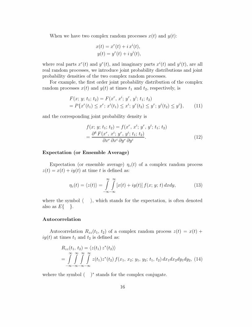
When we have two complex random processes x(t) and y(t):

x(t) = xr(t) + i xi(t),

y(t) = yr(t) + i yi(t),

where real parts xr(t) and yr(t), and imaginary parts xi(t) and yi(t), are allreal random processes, we introduce joint probability distributions and jointprobability densities of the two complex random processes.

For example, the first order joint probability distribution of the complexrandom processes x(t) and y(t) at times t1 and t2, respectively, is

F (x; y; t1; t2) = F (xr, xi; yr, yi; t1; t2)

= Pxr(t1) ≤ xr; xi(t1) ≤ xi; yr(t2) ≤ yr; yi(t2) ≤ yi, (11)

and the corresponding joint probability density is

f(x; y; t1; t2) = f(xr, xi; yr, yi; t1; t2)

=∂4 F (xr, xi; yr, yi; t1; t2)

∂xr ∂xi ∂yr ∂yi. (12)

Expectation (or Ensemble Average)

Expectation (or ensemble average) ηz(t) of a complex random processz(t) = x(t) + iy(t) at time t is defined as:

ηz(t) = 〈z(t)〉 =

∞∫

−∞

∞∫

−∞

[x(t) + iy(t)] f(x; y; t) dxdy, (13)

where the symbol 〈 〉, which stands for the expectation, is often denotedalso as E .

Autocorrelation

Autocorrelation Rzz(t1, t2) of a complex random process z(t) = x(t) +iy(t) at times t1 and t2 is defined as:

Rzz(t1, t2) = 〈z(t1) z∗(t2)〉

=

∞∫

−∞

∞∫

−∞

∞∫

−∞

∞∫

−∞

z(t1)z∗(t2) f(x1, x2; y1, y2; t1, t2) dx1dx2dy1dy2, (14)

wehere the symbol ( )∗ stands for the complex conjugate.

16

Hereafter, we will usually omit sufficies such as zz, for simplicity, whenwe express autocorrelations. Thus, autocorrelations Rxx(t1, t2), Ryy(t1, t2),Rzz(t1, t2), and so on, will be all denoted simply as R(t1, t2), except for cases,when we wish to explicitly specify the random processes under consideration.

Following general properties hold for autocorrelations.

• R(t2, t1) = R∗(t1, t2).

• R(t, t) = 〈| z(t) |2〉 ≥ 0, i.e., real and positive.

• Positive definite, namely,

n∑

i=1

n∑

j=1

aia∗jR(ti, tj) ≥ 0 for any numbers ai (i = 1, 2, · · · , n).

Proof :

0 ≤ 〈|n∑

i=1

aiz(ti) |2〉 =n∑

i=1

n∑

j=1

aia∗j〈z(ti) z∗(tj)〉 =

n∑

i=1

n∑

j=1

aia∗jR(ti, tj).

• An inequality:| R(t1, t2) |2≤ R(t1, t1)R(t2, t2). (15)

Proof :

1. For any complex random variables v and w, we have

〈| v | | w |〉2 ≤ 〈| v |2〉 〈| w |2〉.

Proof :

Since we always have

〈(s | v | + | w |)2〉 = s2〈| v |2〉 + 2s〈| v | | w |〉 + 〈| w |2〉 ≥ 0,

for any real variable s, the discriminant of the above quadraticequation with respect to s must be smaller than or equal to 0, i.e.,

〈| v | | w |〉2 − 〈| v |2〉 〈| w |2〉 ≤ 0,

and, hence,〈| v | | w |〉2 ≤ 〈| v |2〉 〈| w |2〉.

17

2. For any complex random variables v and w, we have

| 〈v w〉 | ≤ 〈| v | | w |〉.Proof :

Let us first prove a general statement that, for any complex ran-dom variable A = a+ ib, where a and b are real random variables,we have

| 〈A〉 | ≤ 〈| A |〉.Let us denote the probability density of A as f(a, b). Then | 〈A〉 |and 〈| A |〉 are expressed as

| 〈A〉 | = |∫ ∫

Af(a, b) dadb |= lim

∆a→0lim

∆b→0|∑∑

Af(a, b)∆a∆b |, (16)

and

〈| A |〉 =∫ ∫

| A | f(a, b) dadb

= lim∆a→0

lim∆b→0

∑∑

| A | f(a, b)∆a∆b

= lim∆a→0

lim∆b→0

∑∑

| Af(a, b)∆a∆b |, (17)

where we replaced the integrtions by the infinite summations,which are performed in the same way in both equations (16) and(17), and we used a property of the probability density f(a, b) inequation (17), that it is always real and greater than or equal tozero.

Now, for any complex numbers B and C, we have

| B + C |≤| B | + | C |,since

| B + C | =√

(B + C)(B + C)∗ =√

| B |2 +B∗C +BC∗+ | C |2

=√

| B |2 +2 | B | | C | cos Φ+ | C |2,where we introduced an angle Φ satisfying

B∗C =| B | | C | eiΦ,is always smaller than | B | + | C |, because cos Φ ≤ 1. Thisrelation is easily extended to the sum of arbitrary number n ofcomplex numbers B1, B, · · ·, Bn, i.e.,

|n∑

i=1

Bi |≤n∑

i=1

| Bi |,

18

because

|n∑

i=1

Bi |=| B1 +n∑

i=2

Bi |≤| B1 | + |n∑

i=2

Bi |=| B1 | + | B2 +n∑

i=3

Bi |

≤| B1 | + | B2 | + |n∑

i=3

Bi |= · · · ≤| B1 | + | B2 | + · · ·+ | Bn | .

Applying the above relation to the summations of equations (16)and (17), we confirm that | 〈A〉 | ≤ 〈| A |〉.This implies that | 〈v w〉 | ≤ 〈| v | | w |〉, since

| v w |=√vwv∗w∗ =

√vv∗

√ww∗ =| v | | w | .

3. From 1. and 2. above, we obtain

| 〈v w〉 |2 ≤ 〈| v | | w |〉2 ≤ 〈| v |2〉 〈| w |2〉,

i.e.,| 〈v w〉 |2 ≤ 〈| v |2〉 〈| w |2〉. (18)

If we adopt here v = z(t1) and w = z∗(t2), then we prove that

| R(t1, t2) |2 ≤ R(t1, t1)R(t2, t2).

Autocovariance

Autocovariance C(t1, t2) of a complex random process z(t) at times t1and t2 is defined as:

C(t1, t2) = R(t1, t2) − η(t1) η∗(t2), (19)

where η(t) ≡ ηz(t) = 〈z(t)〉 is the expectation of z(t) at time t.The autocovariance of z(t) is equal to the autocorrelation of z(t) = z(t)−

η(t), i.e.,C(t1, t2) = Rzz = 〈z(t1) z∗(t2)〉. (20)

In fact,

〈z(t1) z∗(t2)〉 = 〈[z(t1) z∗(t2) − z(t1) η∗(t2) − η(t1) z

∗(t2) + η(t1) η∗(t2)]〉

= R(t1, t2) − η(t1)η∗(t2).

19

Correlation Coefficient

Correlation coefficient r(t1, t2) of a complex random process z(t) at timest1 and t2 is defined as:

r(t1, t2) =C(t1, t2)

√

C(t1, t1)C(t2, t2). (21)

It is evident that

• r(t, t) = 1.

Also, the absolute value of the correlation coefficient is always smaller thanor equal to 1:

• | r(t1, t2) |≤ 1,

since from equations (15) and (20), we have

| C(t1, t2) |2≤ C(t1, t1)C(t2, t2).

Cross–Correlation

Cross–correlation Rxy(t1, t2) of two complex random processes x(t) =xr(t) + i xi(t) and y(t) = yr(t) + i yi(t) at times t1 and t2, respectively, isdefined as:

Rxy(t1, t2) = 〈x(t1) y∗(t2)〉 =∞∫

−∞

∞∫

−∞

∞∫

−∞

∞∫

−∞

x(t1) y∗(t2) f(xr, xi; yr, yi; t1; t2)dx

r dxi dyr dyi, (22)

using the joint probability density of x(t) and y(t), given in equation (12).Following properties hold for cross–correlations.

• Rxy(t2, t1) = R∗yx(t1, t2).

This is evident from the above definition.

• | Rxy(t1, t2) |2 ≤ Rxx(t1, t1)Ryy(t2, t2).This is proven by adopting v = x(t1) and w = y∗(t2) in equation (18).

20

Cross–Covariance

Cross–covariance Cxy(t1, t2) of two complex random processes x(t) andy(t) at times t1 and t2 is defined as:

Cxy(t1, t2) = Rxy(t1, t2) − ηx(t1) η∗y(t2). (23)

Following properties hold for cross-covariances.

• The cross–covariance of x(t) and y(t) is equal to the cross–correlationof x(t) = x(t) − ηx(t) and y(t) = y(t) − ηy(t), i.e.,

Cxy(t1, t2) = Rxy(t1, t2) = 〈x(t1) y∗(t2)〉.

• | Cxy(t1, t2) |2 ≤ Cxx(t1, t1)Cyy(t2, t2).

Cross–Correlation Coefficient

Cross–correlation coefficient rxy(t1, t2) of two complex random processesx(t) and y(t) at times t1 and t2 is defined as:

rxy(t1, t2) =Cxy(t1, t2)

√

Cxx(t1, t1)Cyy(t2, t2). (24)

It is evident that for any cross–correlation coefficient we always have

• | rxy(t1, t2) |≤ 1.

Normal (Gaussian) Process

As an example of the probability density introduced in equations (5), (7),and (8), we consider here probability desnity of a particularly important classof random process, namely normal (or Gaussian) process, which is known tobe a good model of signals from astronomical radio sources, as well as ofnoises produced in antenna–receiving systems or in environments.

Real random process x(t), with expectation η(t) and autocovariance C(t1, t2),is called “normal (or Gaussian) process”, if, at any times t1, t2, · · ·, tn for anyn, random variables x(t1), x(t2), · · ·, x(tn) are jointly normal (or Gaussian),i.e., they are characterized by following probabilty densities.

• First–order Gaussian probability density:

f(x1; t1) =1

σ1

√2π

e−

[x1−η1]2

2σ21 , (25)

21

where η1 ≡ η(t1) and σ21 ≡ C(t1, t1) are expactation and dispersion,

respectively, of x(t) at time t1.

• Second–order Gaussian probability density:

f(x1, x2; t1, t2)

=1

2πσ1σ2

√1 − r2

e− 1

2(1−r2)

(

(x1−η1)2

σ21

−2r(x1−η1)(x2−η2)

σ1σ2+

(x2−η2)2

σ22

)

, (26)

where we introduced notations: η1 ≡ η(t1), η2 ≡ η(t2), σ21 ≡ C(t1, t1),

σ22 ≡ C(t2, t2), and correlation coefficient:

r ≡ C(t1, t2)√

C(t1, t1)C(t2, t2).

• n-th–order Gaussian probability density:

f(x1, · · · , xn; t1, · · · , tn)

=1

√

(2π)n∆e− 1

2

n∑

i=1

n∑

j=1

[xi−ηi]C−1ij

[xj−ηj ]

, (27)

where ηi ≡ η(t1), ηj ≡ η(tj), Cij ≡ C(ti, tj) is autocovariance matrix,C−1ij is its inverse, and ∆ ≡ detCij is its determinant.

When n = 1 and n = 2, equation (27) is reduced to equations (25)and (26). Therefore, the first– and second–order Gaussian probabilitydensities given in equations (25) and (26), respectively, are special casesof the more general expression of the n-th–order normal (or Gaussian)probability density given in equation (27).

Likewise, we can conceive a number of normal (or Gaussian) processeswhich are jointly normal with each other.

• Two real normal processes x(t) and y(t) are called “jointly normal (orGaussian) processes”, if, at any times t1 and t2, random variables x(t1)and y(t2) are jointly normal, i.e., they are characterized by followingjoint probabilty density:

f(x, y; t1, t2)

=1

2πσxσy√

1 − r2xy

e− 1

2(1−r2xy)

(

(x−ηx)2

σ2x

−2 rxy(x−ηx)(y−ηy)

σxσy+

(y−ηy)2

σ2y

)

, (28)

22

where we introduced expectations of x(t1) and y(t2): ηx ≡ ηx(t1) andηy ≡ ηy(t2), dispersions of x(t1) and y(t2): σ2

x ≡ Cxx(t1, t1), σ2y ≡

Cyy(t2, t2), and cross–correlation coefficient:

rxy ≡Cxy(t1, t2)

√

Cxx(t1, t1)Cyy(t2, t2).

Here Cxx(t1, t1), Cyy(t2, t2) and Cxy(t1, t2) are autocovariances andcross–covariance of x(t1) and y(t2), correspondingly.

• An arbitrary number m of normal processes x(1)(t), x(2)(t), · · ·, x(m)(t)are called “jointly normal (or Gaussian) processes”, if, at any times t1,t2, · · ·, tm, random variables x(1)(t1), x(2)(t2), · · ·, x(m)(tm) are jointlynormal, i.e., they are characterized by following joint probabilty den-sity:

f(x(1), · · · , x(m); t1, · · · , tm)

=1

√

(2π)m∆e− 1

2

m∑

i=1

m∑

j=1

[x(i)−η(i)(ti)]C−1(i)(j)

[x(j)−η(j)(tj )]

, (29)

where η(i)(t) is expectation of x(i)(t), C(i)(j) ≡ Cx(i)x(j)(ti, tj) is cross–

covariance matrix, C−1(i)(j) is inverse matrix of C(i)(j), and ∆ ≡ detC(i)(j)

is determinant of C(i)(j).

Of course, equation (28) is a special case of equation (29) with m = 2.

• In the above statement, some random variables among x(1)(t1), x(2)(t2),· · ·, x(m)(tm) could be values of the same normal process taken at dif-ferent times. In such a case, some elements of matrix C(i)(j) are auto-covariances, rather than cross–covariances.

In this sence, joint probability densities of a single normal (or Gaussian)process given in equations (25), (26), and (27) can be regarded asspecial cases of the joint probability density of the jointly normal (orGaussian) processes given in equation (29).

It is not difficult to confirm that the joint probability densities of jointlynormal (or Gaussian) processes given in equations (25) – (29) are consistentwith geneal properties of joint probability densities, as well as with definitionsof the expectation and the covariances, as explained in standard textbooks.For this purpose, we can use well–known integration formulae:

∞∫

−∞

e−a x2

dx =

√

π

a, (30)

23

∞∫

−∞

x e−a x2

dx = 0, (31)

∞∫

−∞

x2 e−a x2

dx =1

2

√

π

a3, (32)

for a > 0.For example, if we take the form of the joint normal (or Gaussian) prob-

ability density given in equation (28), we can confirm following formulae.

•∞∫

−∞f(x, y; t1, t2) dy = f(x ; t1):

∞∫

−∞f(x, y; t1, t2) dy

=1

2πσxσy√

1 − r2xy

∞∫

−∞

e− 1

2(1−r2xy)

(

(x−ηx)2

σ2x

−2 rxy(x−ηx)(y−ηy)

σxσy+

(y−ηy)2

σ2y

)

dy

=1

2πσx√

1 − r2xy

∞∫

−∞

e− 1

2(1−r2xy)

(

(x−ηx)2

σ2x

−2 rxy(x−ηx)

σxy′+y′2

)

dy′

=1

2πσx√

1 − r2xy

∞∫

−∞

e− 1

2(1−r2xy)

[

(1−r2xy)(x−ηx)2

σ2x

+(y′−rxyx−ηx

σx)2]

dy′

=1

2πσx√

1 − r2xy

e−

(x−ηx)2

2 σ2x

∞∫

−∞

e− y′′

2

2 (1−r2xy) dy′′

=1

σx√

2 πe−

(x−ηx)2

2 σ2x = f(x ; t1), (33)

in view of equation (30), where we introduced variable transformations:

y′ =y − ηyσy

, y′′ = y′ − rxyx− ηxσx

.

• Expectation:

〈x〉 =

∞∫

−∞

∞∫

−∞

x f(x, y; t1, t2) dx dy =

∞∫

−∞

x

∞∫

−∞

f(x, y; t1, t2) dy dx

=

∞∫

−∞

xf(x ; t1) dx =1

σx√

2 π

∞∫

−∞

x e−

(x−ηx)2

2 σ2x dx

24

=1

σx√

2 π

∞∫

−∞

[(x− ηx) + ηx] e−

(x−ηx)2

2 σ2x dx

=ηx

σx√

2 π

∞∫

−∞

e−

(x−ηx)2

2 σ2x dx = ηx, (34)

in view of equations (30) and (31).

• Covariance:

〈(x− ηx) (y − ηy)〉

=

∞∫

−∞

∞∫

−∞

(x− ηx) (y − ηy) f(x, y; t1, t2) dx dy

=1

2πσxσy√

1 − r2xy

×∞∫

−∞

∞∫

−∞

(x− ηx) (y − ηy) e− 1

2(1−r2xy)

(

(x−ηx)2

σ2x

−2 rxy(x−ηx)(y−ηy)

σxσy+

(y−ηy)2

σ2y

)

dx dy

=σx σy

2π√

1 − r2xy

∞∫

−∞

∞∫

−∞

x′ y′ e− 1

2(1−r2xy)

(x′2−2rxy x′ y′+y′2)dx′ dy′

=σx σy

2π√

1 − r2xy

∞∫

−∞

∞∫

−∞

(x′′ + rxy y′′) y′′ e

− 1

2(1−r2xy)

[x′′2+(1−r2xy) y′′2]dx′′ dy′′

=σx σy rxy

2π√

1 − r2xy

∞∫

−∞

e− x′′

2

2(1−r2xy) dx′′

∞∫

−∞

y′′2e−

y′′2

2 dy′′

=σx σy rxy

2π√

1 − r2xy

√

2π(1 − r2xy)

√2π = rxy σx σy = Cxy(t1, t2), (35)

in view of equations (30), (31), and (32), where we introduced variabletransformations:

x′ =x− ηxσx

, y′ =y − ηyσy

,

x′′ = x′ − rxy y′, y′′ = y′.

In following discussions, we will mainly use general properties of expectationsand correlations, without specifying explicit forms of probability densities.However, when necessary, we will assume jointly normal (or Gaussian) pro-cesses, and explicitly use expressions of the normal probability density givenin equations (25) – (29).

25

1.2.2 Random Processes in Linear Systems

Definition of Linear Systems

Let us consider a system of two complex functions x(t) and y(t) of timet, which are related with each other by an operator L:

y(t) = L[x(t)], (36)

where x(t) is called “input” and y(t) is called “output” of the operator L.Such a system is called “linear system”, if the operator L satisfies

L[a1 x1(t) + a2 x2(t)] = a1L[x1(t)] + a2L[x2(t)], (37)

for any complex coefficients a1, a2 and for any functions x1(t), x2(t).The linear system is also called as “linear filter”, which linearly “filters”

the input x(t) to yield the output y(t).

Impulse Response

If the input of an operator L is a delta function δ(t) of time t, the outputis called “impulse response” of the operator, which we denote as h(t):

h(t) = L[δ(t)]. (38)

Here, we introduce “convolution” f(t) ∗ g(t) of functions f(t) and g(t),which is defined by a following infinite integration:

f(t) ∗ g(t) =

∞∫

−∞

f(t− α) g(α) dα, (39)

where symbol “∗” stands for the operation of the convolution. Convolutionhas following properties:

f(t) ∗ g(t) = g(t) ∗ f(t) (commutative),

because

g(t)∗f(t) =

∞∫

−∞

g(t−β) f(β) dβ =

∞∫

−∞

f(β) g(t−β) dβ =

∞∫

−∞

f(t−α) g(α) dα,

where we used a transformation of the argument of the integration: α = t−βand hence dβ = −dα,

26

and

f(t) ∗ g(−t) =

∞∫

−∞

f(t− β) g(−β) dβ =

∞∫

−∞

f(t+ α) g(α) dα,

where we used α = −β and dβ = −dα.

Then, the output of the linear system can be represented as a convolutionof the input and the impulse response, i.e.,

y(t) = x(t) ∗ h(t) =

∞∫

−∞

x(t− α) h(α) dα. (40)

This equation is easily proven, based on the definition of the delta function,in the following way:

y(t) = L[x(t)] = L[

∞∫

−∞

x(β) δ(t− β) dβ] =

∞∫

−∞

x(β)L[δ(t− β)] dβ

=

∞∫

−∞

x(β) h(t− β) dβ =

∞∫

−∞

x(t− α) h(α) dα = x(t) ∗ h(t).

Note that L operates only on a function of time t.

Linear Systems with Random Processes as Inputs

Hereafter, we will consider linear systems having random processes asinputs. Then, we have following general properties.

• If x(t) and y(t) are input and output of a linear system, their expec-tations 〈x(t)〉 and 〈y(t)〉 are also related with each other as input andoutput of the same linear system, i.e.,

〈L[x(t)]〉 = L[〈x(t)〉],or

〈x(t) ∗ h(t)〉 = 〈x(t)〉 ∗ h(t),or

ηy(t) = L[ηx(t)]. (41)

Proof :

〈x(t) ∗ h(t)〉 = 〈∞∫

−∞

x(t− α) h(α) dα〉 =

∞∫

−∞

〈x(t− α)〉 h(α) dα

= 〈x(t)〉 ∗ h(t).

27

Note that the impulse response h(t) is a deterministic function of time,and, hence, not affected by the ensemble average.

• Autocorrelation of the output:

Ryy(t1, t2) = Rxx(t1, t2) ∗ h(t1) ∗ h∗(t2),or

Ryy(t1, t2) =

∞∫

−∞

∞∫

−∞

Rxx(t1 − α, t2 − β) h(α) h∗(β) dαdβ. (42)

Proof :

1. Cross–correlation of the input and the output is

Rxy(t1, t2) = 〈x(t1) y∗(t2)〉 = 〈x(t1) x∗(t2) ∗ h∗(t2)〉= 〈x(t1) x∗(t2)〉 ∗ h∗(t2) = Rxx(t1, t2) ∗ h∗(t2),or

Rxy(t1, t2) =

∞∫

−∞

Rxx(t1, t2 − β) h∗(β) dβ.

2. Autocorrelation of the output is

Ryy(t1, t2) = 〈y(t1) y∗(t2)〉 = 〈x(t1) ∗ h(t1) y∗(t2)〉= 〈x(t1) y∗(t2)〉 ∗ h(t1) = Rxy(t1, t2) ∗ h(t1),or

Ryy(t1, t2) =

∞∫

−∞

Rxy(t1 − α, t2) h(α) dα.

3. From 1. and 2. above, we have

Ryy(t1, t2) = Rxx(t1, t2) ∗ h∗(t2) ∗ h(t1)= Rxx(t1, t2) ∗ h(t1) ∗ h∗(t2),or

Ryy(t1, t2) =

∞∫

−∞

∞∫

−∞

Rxx(t1 − α, t2 − β) h(α) h∗(β) dαdβ.

1.2.3 Stationary Random Processes

Definitions

28

• A random process z(t) is called “stationary” (or, more specifically,“wide–sense stationary”), if the expectation does not depend on time,and the autocorrelation is a function of time difference only:

〈z(t)〉 = η = const,

〈z(t1) z∗(t2)〉 = R(τ), (43)

where τ ≡ t1 − t2.

• Random processes x(t) and y(t) are called “jointly stationary”, if bothof them are stationary, and their cross–correlation is a function of timedifference only:

〈x(t1) y∗(t2)〉 = Rxy(τ), (44)

where τ ≡ t1 − t2.

Of course, it is not easy to find actual physical processes which strictly satisfythese conditions. For example, some of quasars or astronomical masers areknown to exihit significant time variations in yearly, or shorter, time scales.In a practical sense, however, physical processes are well approximated bythe stationary random processes, if equations (43) and (44) are fulfilled dur-ing time scales, which are sufficient to estimate their statistical properties(see discussions on ergodicity in section 1.2.4). In this sense, many physicalprocesses can be successfully modeled as stationary random processes.

Properties

Following formulae can be easily derived, by applying general propertiesof correlations, covariances, and so on, to the particular case of the stationaryrandom processes as defined above.

• R(−τ) = R∗(τ).

• R(0) = 〈| z(t) |2〉 ≥ 0.

• Positive definiteness:

n∑

i=1

n∑

j=1

ai a∗jR(ti − tj) ≥ 0, for any ai.

• | R(τ) |≤ R(0).

• C(τ) = R(τ)− | η |2, autocovariance.

29

• r(τ) = C(τ)/C(0), correlation coefficient.

• | r(τ) |≤ 1.

• Rxy(−τ) = R∗yx(τ).

• | Rxy(τ) |2≤ Rxx(0)Ryy(0).

• Cxy(τ) = Rxy(τ) − ηx η∗y, cross–covariance.

• rxy = Cxy(τ)/√

Cxx(0)Cyy(0), cross–correlation coefficient.

• | rxy(τ) |≤ 1.

1.2.4 Ergodicity

How can we estimate various statistical properties of a random process, ifwe are given with a single sample of time series only, which is an outcome ofa single trial?

• Definition.A random process z(t) is called “ergodic” if its ensemble averages areequal to appropriate time averages.

This implies that we can estimate any statistical property ofz(t), using time average of the single sample, if the randomprocess is ergodic.

• Mean–ergotic process.A random process z(t), with constant expectation:

η = 〈z(t)〉,

is called “mean–ergotic”, if its time average tends to η as averagingtime tends to infinity:

ηT =1

2T

T∫

−T

z(t)dt → η as T → ∞.

• A condition for the mean–ergotic process.It is evident that

〈ηT 〉 =1

2T

T∫

−T

〈z(t)〉dt = η.

30

Therefore, z(t) is mean–ergotic, if its “variance”, or “dispersion”, σ2T

tends to 0 as T → ∞, i.e.,

σ2T ≡ 〈| ηT − η |2〉 → 0 as T → ∞.

Since

σ2T = 〈| ηT − η |2〉 =

1

(2T )2

T∫

−T

T∫

−T

〈(z(t1) − η) (z(t2) − η)∗〉 dt1 dt2

=1

(2T )2

T∫

−T

T∫

−T

C(t1, t2) dt1 dt2,

where C(t1, t2) is the autocovariance, and we used here equation (20),the above condition is equivalent to

1

(2T )2

T∫

−T

T∫

−T

C(t1, t2) dt1 dt2 → 0 as T → ∞.

• In the stationary random case.If z(t) is a stationary random process, and, therfore, the autocovarianceis a function of time diffference τ = t1 − t2 only:

C(t1, t2) = C(τ),

the double integral in the above condition is reduced to a single integral:

1

2T

2T∫

−2T

C(τ)

(

1 − | τ |2T

)

dτ → 0 as T → ∞, (45)

because

T∫

−T

T∫

−T

C(t1, t2) dt1 dt2 =

2T∫

−2T

C(τ)(2T− | τ |) dτ, (46)

as we can easily see from Figure 8. In fact, in the rectangular rangeof integration −T ≤ t1 ≤ T and −T ≤ t2 ≤ T in Figure 8, theautocovariance C(τ) is constant along a line t1 − t2 = τ , and an area ofthe hatched region, put between two lines t1−t2 = τ and t1−t2 = τ+∆τis nearly equal to the area of the enclosing parallelogram, which is equalto (2T− | τ |) ∆τ , in the linear approximation with respect to small∆τ .

31

t1

t2

τ+∆ττ

T

T

-T

-T

t1-t2=-2T

t1-t2=t1-t2=t1-t2=2T τ+∆τ

τ

0

2T-|τ|

Figure 8: Geometry of the integration.

• Correlation–ergodic process.A stationary random process z(t) with an autocorrelation

R(ξ) = 〈z(t + ξ) z∗(t)〉,

is called “correlation–ergodic”, if the corresponding process uξ(t):

uξ(t) = z(t + ξ) z∗(t),

is mean–ergotic, i.e., if

RT ≡ 1

2T

T∫

−T

uξ(t) dt→ R(ξ) as T → ∞.

Similarly to the case of the mean–ergotic process, z(t) is correlation–ergotic, if the variance, or dispersion, σ2

RT≡ 〈| RT − R(ξ) |2〉 tends to

0 as T → ∞, or, equivalently, if an autocovarinace of uξ(t):

Cuu(τ) = Ruu(τ) − R2(ξ),

32

where Ruu(τ) is an autocorrelation of uξ(t):

Ruu(τ) = 〈uξ(t + τ) u∗ξ(t)〉 = 〈z(t + ξ + τ) z∗(t + τ) z∗(t+ ξ) z(t)〉,

satisfies the condition in equation (45) for any ξ, i.e.,

1

2T

2T∫

−2T

Cuu(τ)

(

1 − | τ |2T

)

dτ → 0 as T → ∞. (47)

For actual physical processes, which are approximated by the stationaryrandom processes, it is likely that autocovariances are finite everywhere andtend to 0 when τ → ±∞. Therefore, equations (45) and (47) appear wellsatisfied in the most cases. In the followings, we assume that these equationsare fulfilled, and, hence, we can estimate both expectation and correlation ofour physical process in terms of the time averaging of a single sample.

It is known that the power or the correlation of a moderately strongsignal from an astronomical radio source, which is estimated by time averag-ing in a square–law detector or in a correlator, usually reaches a sufficientlyhigh signal–to–noise ratio, that means a small enough dispersion, after aver-aging during seconds to hours, depending on telescope or array sensitivity.The detected power or correlation is usually almost time–invariant duringtime–scales from hours to months. Therefore, radio astronomical data aremostly consistent with assumptions of the stationary random process andthe ergodicity.

1.2.5 Stationary Random Processes in Linear Systems

Let us consider cases when inputs of linear systems are stationary randomprocesses. Then, we have following properties.

• If an input x(t) in a linear system y(t) = L[x(t)] is a stationary randomprocess, then an output y(t) is also a stationary random process.

Proof :

1. Expectation ηy(t) of the output y(t) is constant in time, because

ηy(t) =

∞∫

−∞

ηx(t− α) h(α) dα = ηx

∞∫

−∞

h(α) dα = const,

33

since x(t) is stationary, and hence, ηx(t) = ηx is constant in time.Thus, we have

ηy = ηx

∞∫

−∞

h(α) dα. (48)

2. Autocorrelation Ryy(t1, t2) of the output y(t) is a function of timedifference τ = t1 − t2 only, because

Ryy(t1, t2) =

∞∫

−∞

∞∫

−∞

Rxx(t1 − α, t2 − β) h(α) h∗(β) dαdβ

=

∞∫

−∞

∞∫

−∞

Rxx(τ − α + β) h(α) h∗(β) dαdβ,

since x(t) is stationary, and hence,

Rxx(t1 − α, t2 − β) = Rxx(t1 − α− (t2 − β)) = Rxx(τ − α + β).

Then, the above formula is now expressed as:

Ryy(τ) = Rxx(τ) ∗ h(τ) ∗ h∗(−τ). (49)

• If an input x(t) in a linear system y(t) = L[x(t)] is a stationary randomprocess, then the input x(t) and the output y(t) are jointly stationary.

Proof :

1. We have proven above that, if the input is stationary, then theoutput is also stationary, i.e., both x(t) and y(t) are stationary.

2. Cross–correlation Rxy(t1, t2) of the input x(t) and the output y(t)is a function of time difference τ = t1 − t2 only, because

Rxy(t1, t2) = 〈x(t1) y∗(t2)〉 =

∞∫

−∞

〈x(t1) x∗(t2 − α)〉 h∗(α) dα

=

∞∫

−∞

Rxx(τ + α) h∗(α) dα = Rxx(τ) ∗ h∗(−τ).

Thus, we haveRxy(τ) = Rxx(τ) ∗ h∗(−τ). (50)

34

• Likewise, we can prove an equation:

Ryy(τ) = Rxy(τ) ∗ h(τ), (51)

which, together with equation (50), offers another derivation of equa-tion (49).

• If x1(t) and x2(t) are jointly stationary random processes, then out-puts y1(t) and y2(t), which are obtained from x1(t) and x2(t) througharbitrary linear operators L1 and L2, respectively, are also jointly sta-tionary.

Proof :

Let the two linear operators L1 and L2 correspond to impulse responsesh1(t) and h2(t), respectively. Then we have

y1(t) = L1[x1(t)] = x1(t) ∗ h1(t) =

∞∫

−∞

x1(t− α) h1(α) dα,

y2(t) = L2[x2(t)] = x2(t) ∗ h2(t) =

∞∫

−∞

x2(t− α) h2(α) dα.

Both y1(t) and y2(t) are, of course, stationary, and their cross–correlation:

Ry1y2(t1, t2) = 〈y1(t1) y∗2(t2)〉

=

∞∫

−∞

∞∫

−∞

〈x1(t1 − α) x∗2(t2 − β)〉 h1(α) h∗2(β) dαdβ

=

∞∫

−∞

∞∫

−∞

Rx1x2(τ − α + β) h1(α) h∗2(β) dαdβ,

is a function of time difference τ = t1 − t2 only. This proves the jointstationarity of y1(t) and y2(t), and yields

Ry1y2(τ) = Rx1x2(τ) ∗ h1(τ) ∗ h∗2(−τ). (52)

1.2.6 Spectra of Stationary Random Processes

Definitions

• Fourier transform S(ω) of an autocorrelation R(τ) of a stationary ran-dom process is called “power spectrum” (or “spectral density”) of theprocess. Here, ω is an angular frequency, which is related to a linear

35

frequency ν as ω = 2πν. Thus, the power spectrum and the autocor-relation are related to each other by the Fourier– and inverse Fouriertransforms:

S(ω) =

∞∫

−∞

R(τ)e−iωτ dτ, (53)

R(τ) =1

2π

∞∫

−∞

S(ω)eiωτ dω. (54)

Hereafter, we express a Fourier transform pair by a symbol “⇔”. Then,

S(ω) ⇔ R(τ).

• Fourier transform Sxy(ω) of a cross–correlation Rxy(τ) of jointly sta-tionary random processes x(t) and y(t) is called “cross–power spec-trum”. Thus,

Sxy(ω) =

∞∫

−∞

Rxy(τ)e−iωτ dτ, (55)

Rxy(τ) =1

2π

∞∫

−∞

Sxy(ω)eiωτ dω, (56)

andSxy(ω) ⇔ Rxy(τ).

Note that convergence of Fourier integrals in equations (53) and (55), andtherefore in their inverses in equations (54) and (56), too, is usually guaran-teed, since, for actual physical processes, R(τ) and Rxy(τ) are mostly finiteeverywhere, and tend to zero as τ → ±∞.

Properties

• Power 〈| z(t) |2〉 of a stationary random process z(t) is equal to anintegrated power spectrum over the whole frequency range:

〈| z(t) |2〉 = R(0) =1

2π

∞∫

−∞

S(ω) dω =

∞∫

−∞

S(ω) dν, (57)

where ν = ω/(2π) is a frequency, corresponding to the angular fre-quency ω.

36

• Power spectrum S(ω) is a real function.

Proof :

Since R(−τ) = R∗(τ),

S∗(ω) =

∞∫

−∞

R∗(τ)eiωτ dτ =

∞∫

−∞

R(−τ)eiωτ dτ =

∞∫

−∞

R(τ)e−iωτ dτ = S(ω).

• For any cross–power spectrum, Sxy(ω) = S∗yx(ω).

Proof :

Since Rxy(−τ) = R∗yx(τ),

S∗yx(ω) =

∞∫

−∞

R∗yx(τ)e

iωτ dτ =

∞∫

−∞

Rxy(−τ)eiωτ dτ =

∞∫

−∞

Rxy(τ)e−iωτ dτ

= Sxy(ω).

• A power spectrum S(ω) corresponding to a real autocorrelation R(τ)is an even function of ω (see Figure 9):

S(−ω) = S(ω). (58)

0 ω

S(ω)

Figure 9: Power spectrum is even when autocorrelation is real.

Proof :

Since, in this case, R(−τ) = R(τ) (the real autocorrelation is an evenfunction of τ),

S(−ω) =

∞∫

−∞

R(τ)eiωτ dτ =

∞∫

−∞

R(−τ)eiωτ dτ =

∞∫

−∞

R(τ)e−iωτ dτ = S(ω).

37

• A cross–power spectrum corresponding to a real cross–correlation sat-isfies

Sxy(−ω) = Syx(ω), (59)

and, therefore, is Hermitian symmetric:

Sxy(−ω) = S∗xy(ω), (60)

(see Figure 10).

ω ω0 0

Re Sxy(ω) Im Sxy(ω)

Figure 10: Cross–power spectrum is Hermitian symmetric (i.e., real part iseven and imaginary part is odd) when cross–correlation is real.

Proof :

Since, in this case, Rxy(−τ) = Ryx(τ),

Sxy(−ω) =

∞∫

−∞

Rxy(τ)eiωτ dτ =

∞∫

−∞

Rxy(−τ)e−iωτ dτ =

∞∫

−∞

Ryx(τ)e−iωτ dτ

= Syx(ω),

and, in view of the general property Sxy(ω) = S∗yx(ω), we also have

Sxy(−ω) = S∗xy(ω).

• Real autocorrelation can be described solely by the positive frequencyrange of the power spectrum.

Proof :

Since S(ω) = S(−ω), in this case,

R(τ) =1

2π

∞∫

−∞

S(ω)eiωτ dω =1

2π

0∫

−∞

S(ω)eiωτ dω +

∞∫

0

S(ω)eiωτ dω

38

=1

2π

∞∫

0

[S(−w)e−iωτ + S(ω)eiωτ ] dω =1

2π

∞∫

0

S(ω)[e−iωτ + eiωτ ] dω

=1

π

∞∫

0

S(ω) cos(ωτ) dω =1

π<

∞∫

0

S(ω)eiωτ dω

. (61)

• Real cross–correlation can be described solely by the positive frequencyrange of the cross–power spectrum.

Proof :

Since Sxy(−ω) = S∗xy(ω), in this case,

Rxy(τ) =1

2π

∞∫

−∞

Sxy(ω)eiωτ dω =1

2π

0∫

−∞

Sxy(ω)eiωτ dω +

∞∫

0

Sxy(ω)eiωτ dω

=1

2π

∞∫

0

[Sxy(−w)e−iωτ + Sxy(ω)eiωτ ] dω

=1

2π

∞∫

0

[S∗xy(ω)e−iωτ + Sxy(ω)eiωτ ] dω

=1

π<

∞∫

0

Sxy(ω)eiωτ dω. (62)

• White noise: if the spectrum is flat throughout the whole frequencyrange, then the correlation is proportional to the delta function of τ .

If S(ω) = S = const, then

R(τ) =1

2π

∞∫

−∞

S(ω)eiωτ dω = S1

2π

∞∫

−∞

eiωτ dω = S δ(τ). (63)

If Sxy(ω) = Sxy = const, then

Rxy(τ) =1

2π

∞∫

−∞

Sxy(ω)eiωτ dω = Sxy1

2π

∞∫

−∞

eiωτ dω = Sxy δ(τ). (64)

Here we used a formula

∞∫

−∞

eiωτ dω = 2πδ(τ), (65)

39

which is known as one of the definitions of the delta function.

Thus, if spectra of random processes are completely flat (white), thentheir correlations are non–zero, only when τ = 0.

• Convolution theorem: Fourier transform of a convolution of two func-tions is equal to a product of Fourier transforms of those functions, i.e.,if a(τ) ⇔ A(ω) and b(τ) ⇔ B(ω), then

a(τ) ∗ b(τ) ⇔ A(ω)B(ω). (66)

Proof :∞∫

−∞

a(τ) ∗ b(τ) e−iωτ dτ =

∞∫

−∞

∞∫

−∞

a(τ − α) b(α) e−iωτ dα dτ

=

∞∫

−∞

∞∫

−∞

a(τ ′) e−iωτ′

b(τ ′′) e−iωτ′′

dτ ′ dτ ′′ = A(ω)B(ω),

where we introduced transformations τ ′ = τ − α and τ ′′ = α.

• Another convolution theorem holds for a product of functions a(τ) andb(τ):

a(τ) b(τ) ⇔ 1

2πA(ω) ∗B(ω), (67)

because∞∫

−∞

a(τ) b(τ) e−iωτ dτ

=1

(2π)2

∞∫

−∞

∞∫

−∞

A(ω′) eiω′τ dω′

∞∫

−∞

B(ω′′) eiω′′τ dω′′

e−iωτ dτ

=1

(2π)2

∞∫

−∞

∞∫

−∞

A(ω′)B(ω′′)

∞∫

−∞

e−i(ω−ω′−ω′′) τ dτ

dω′ dω′′

=1

2π

∞∫

−∞

∞∫

−∞

A(ω′)B(ω′′) δ(ω − ω′ − ω′′) dω′ dω′′

=1

2π

∞∫

−∞

A(ω − ω′)B(ω′) dω′ =1

2πA(ω) ∗B(ω),

we used here the relation∞∫

−∞

e−iωτ dτ =

∞∫

−∞

eiωτ dτ = 2πδ(ω).

40

• Shift theorem:If a(τ) ⇔ A(ω), then

a(τ − τ0) ⇔ A(ω) e−iωτ0,

a(τ)eiω0τ ⇔ A(ω − ω0). (68)

Proof :

∞∫

−∞

a(τ − τ0) e−iωτ dτ =

∞∫

−∞

a(τ ′) e−iω(τ ′+τ0) dτ ′

=

∞∫

−∞

a(τ ′)e−iωτ′

dτ ′

e−iωτ0 = A(ω)e−iωτ0,

and,

∞∫

−∞

a(τ)eiω0τ e−iωτ dτ =

∞∫

−∞

a(τ)e−i(ω−ω0)τ dτ = A(ω − ω0). (69)

1.2.7 Spectra of Outputs of Linear Systems

Let us call a Fourier transform H(ω) of an impulse response h(t) of a linearsystem as the “system function”:

H(ω) =

∞∫

−∞

h(t) e−iωt dt, (70)

or

H(ω) ⇔ h(t).

For the system function, we have

H∗(ω) ⇔ h∗(−t),

because

H∗(ω) =

∞∫

−∞

h∗(t)eiωt dt =

∞∫

−∞

h∗(−t)e−iωt dt.

Now, let us consider stationary random processes as inputs of a linearsystem y(t) = L[x(t)] with the impulse response h(t) and the system functionH(ω).

41

• Expectation of the output.

ηy = ηx

∞∫

−∞

h(α) dα = ηxH(0). (71)

• Power spectra of the output Syy(ω) and the inputs Sxx(ω) are mutuallyrelated to each other as

Syy(ω) = Sxx(ω) | H(ω) |2 . (72)

Proof :

In view of the convolution theorem given in equation (66), and prop-erties of correlations,

Rxy(τ) = Rxx(τ) ∗ h∗(−τ) ⇔ Sxy(ω) = Sxx(ω)H∗(ω),

Ryy(τ) = Rxy(τ) ∗ h(τ) ⇔ Syy(ω) = Sxy(ω)H(ω),

and, hence

Ryy(τ) = Rxx(τ) ∗ h(τ) ∗ h∗(−τ) ⇔ Syy(ω) = Sxx(ω) | H(ω) |2 .

• Autocorrelations of the outputs:

Ryy(τ) = 〈y(t+ τ) y∗(t)〉 =1

2π

∞∫

−∞

Sxx(ω) | H(ω) |2 eiωτ dω,

and, in particular,

Ryy(0) = 〈| y(t) |2〉 =1

2π

∞∫

−∞

Sxx(ω) | H(ω) |2 dω. (73)

• If the impulse response h(t) is real, then

H∗(ω) =

∞∫

−∞

h(t)eiωt dt = H(−ω), (74)

and, therefore, | H(ω) |2 is an even function of ω, because

| H(−ω) |2= H(−ω)H∗(−ω) = H∗(ω)H(ω) =| H(ω) |2 . (75)

• Cross–power spectrum of outputs y1(t) = x1(t) ∗ h1(t) and y2(t) =x2(t) ∗ h2(t) of jointly stationary inputs x1(t) and x2(t) through twolinear systems with impulse responses h1(t) and h2(t).

42

As we saw earlier in equation (52), the cross–correlation Ry1y2(τ) ofthe outputs is expressed through the cross–correlation of the inputsRx1x2(τ) as

Ry1y2(τ) = Rx1x2(τ) ∗ h1(τ) ∗ h∗2(−τ).Therefore, the convolution theorem in equation (66) gives us the cross–power spectrum:

Sy1y2(ω) = Sx1x2(ω)H1(ω)H∗2 (ω), (76)

where Sx1x2(ω) ⇔ Rx1x2(τ) is a cross–power spectrum of the inputs.

• Cross–correlation of the outputs.

Ry1y2(τ) = 〈y1(t + τ) y∗2(t)〉 =1

2π

∞∫

−∞

Sx1x2(ω)H1(ω)H∗2(ω)eiωτ dω,

and, hence,

Ry1y2(0) = 〈y1(t) y∗2(t)〉 =

1

2π

∞∫

−∞

Sx1x2(ω)H1(ω)H∗2(ω) dω. (77)

1.2.8 Two Designs of Spectrometers

As an example of applications of the theory of the stationary random process,let us consider principles of two types of spectrometers which have beenwidely used in the radio astronomy (Figures 11 and 12).

In the filterbank spectrometer (Figure 11), received voltage from a radiosource is equally fed to n identical analog narrow–band BPF’s (band–pass–filters), which are called “filterbank” with successive center frequences ν1, ν2,· · ·, νn. Outputs of the BPF’s are squared and averaged by SQ (square–law)detectors and resultant powers yield a spectral shape of the source at theabove frequencies.

LO

BPF ν1 SQ Detector

BPF νn-1 SQ Detector

BPF ν2 SQ Detector

BPF ν3 SQ Detector

BPF νn SQ Detector

Spectrum

Figure 11: Basic design of a filterbank spectrometer.

43

In the autocorrelation spectrometer (Figure 12), on the other hand, thereceived voltage is first digitized by an analog–to–digital converter (A/D),and then equally divided into two digital signals, which are fed to n multi-pliers and integrators, one directly, and another with successive time delays0, τ , 2τ , · · ·, (n − 1)τ . The resultant ‘autocorrelation’ as a function of timedelay is then Fourier transformed, and converted to a power spectrum.

LO

A/D

τ

τ

τ

τ

τ

IntegratorMultiplier

IntegratorMultiplier

IntegratorMultiplier

IntegratorMultiplier

IntegratorMultiplier

IntegratorMultiplierSpectrum

Fou

rier

Tra

nsfo

rmat

ion

Figure 12: Basic design of an autocorrelation spectrometer.

The principles of the two designs look quite different. Do they reallyproduce the same spectrum?

As far as the ergodicity holds, it is clear that the autocorrelation spec-trometer must closely approximate the calculation of the power spectrum ofthe input signal (received voltage) as the Fourier transform of the autocor-relation, as we have described so far.

For the filterbank spectrometer, let us consider i-th narrow–band BPF asa linear system, which has an input stationary random process x(t), whichis the received voltage in this case, an output yi(t), and an impulse responsehi(t), corresponding to a rectangular sytem function Hi(ω):

Hi(ω) =

√

2π∆ω

ωi − ∆ω2

≤ ω ≤ ωi +∆ω2,

0 otherwise,

where ωi = 2πνi is the i-th center angular frequency, and ∆ω is the frequencybandwidth of the BPF. If the power spectrum of the input is Sxx(ω), then,according to equation (72), the power spectrum of the output Syy(ω) is

Syy(ω) = Sxx(ω) | Hi(ω) |2,

(Figure 13). Since, in view of the ergodicity, the time averaging in a square–

44

0

Sxx(ω)

ω ω ω

2π∆ω

Hi(ω) Syy(ω)

0 0

∆ω ∆ω

ωi ωi

Figure 13: Band–pass filter passes a segment of the input power spectrum.

law detector must yield the power, or the autocorrelation at τ = 0, of theoutput signal, if the averaging time is sufficiently long, we obtain

〈| yi(t) |2〉 =1

2π

∞∫

−∞

Syy(ω) dω =1

2π

∞∫

−∞

Sxx(ω) | Hi(ω) |2 dω

=1

∆ω

ωi+∆ω2

∫

ωi−∆ω2

Sxx(ω) dω.

This “power passed by a BPF” is nothing but a mean of the power spec-trum of the received voltage Sxx(ω), involved in the spectral range ωi −∆ω2

≤ ω ≤ ωi + ∆ω2

. Therefore, if ∆ω is sufficiently narrow, and Sxx(ω)is continuous around ωi, then we approximately have

〈| yi(t) |2〉 ' Sxx(ωi).

Thus two spectrometers really yield the same power spectrum of the receivedvoltage.

This example gives us a clear feel, that the power spectrum, defined asa Fourier transform of the autocorrelation of the input signal, is really a“spectrum of the power” of the signal.

1.2.9 Fourier Transforms of Stationary Random Processes

So far, we have considered Fourier transformation of correlations of the sta-tionary random processes. Now, let us proceed to considerations of theFourier transformation of the stationary random processes themselves.

Assume that a Fourier integral of a random process z(t) is expressed as

Z(ω) =

∞∫

−∞

z(t) e−iωt dt. (78)

45

Since z(t) is a random process in time t, it is natural to consider that Z(ω)is a random process in angular frequency ω, i.e., it is a function of ω, and itsvalue at any ω is a random variable, which may vary from trial to trial.

If we apply the inverse Fourier transform to equation (78), we would have

z(t) =1

2π

∞∫

−∞

Z(ω) eiωt dω, (79)

i.e., we could express any random process in time t as a superposition ofinfinite number of frequency components, which are themselves random pro-cesses in angular frequency ω.

Strictly speaking, however, we must be aware that the convergence ofthe intrgrals in equations (78) and (79) is not, in general, guaranteed, sincethe random processes may have finite amplitudes from the infinite past tothe infinite future. Of course, we could restrict the actual integration rangeto −T < t ≤ T with sufficiently large T . In fact, durations of actualphysical processes are most likely to be shorter than the age of our Universe.However, a too strong emphasis on this point may cause difficulties when werequire stationarity to the random processes. Special integral forms are oftenintroduced in the literature to assure the convergence. We will, however,just assume some kind of convergence of the above integrals, without beingheavily involved in the mathematical strictness. Instead, we will concentrateour attentions to several simple but useful statistical relations between therandom process z(t) and its Fourier transform Z(ω).

Properties of Fourier transforms of the random processes.

• Expectation of Z(ω) is a Fourier transform of the expectation η(t) ofz(t).

Proof :

Taking ensemble average of the two sides of the Fourier transformationin equation (78), we have

〈Z(ω)〉 =

∞∫

−∞

〈z(t)〉 e−iωt dt =

∞∫

−∞

η(t) e−iωt dt.

• If z(t) is a stationary random process, the expectaion of Z(ω) has adelta–function form with respect to ω.

46

Proof :

Since〈z(t)〉 = η = const,

we have

〈Z(ω)〉 =

∞∫

−∞

η e−iωt dt = 2π η δ(ω), (80)

according to equation (65).

• An autocorrelation of Z(ω), defined as 〈Z(ω1)Z∗(ω2)〉, is related to

a two–dimensional Fourier transform Γ(ω1, ω2) of an autocorrelationR(t1, t2) = 〈z(t1) z∗(t2)〉 of z(t), which is

Γ(ω1, ω2) =

∞∫

−∞

∞∫

−∞

R(t1, t2) e−i(ω1t1+ω2t2) dt1 dt2,

by a formula:〈Z(ω1)Z

∗(ω2)〉 = Γ(ω1, −ω2). (81)

Proof :

From equation (78),

〈Z(ω1)Z∗(ω2)〉 =

∞∫

−∞

∞∫

−∞

〈z(t1) z∗(t2)〉 e−i(ω1t1−ω2t2) dt1 dt2

=

∞∫

−∞

∞∫

−∞

R(t1, t2) e−i(ω1t1−ω2t2) dt1 dt2 = Γ(ω1, −ω2).

• If z(t) is a stationary random process, having a power spectrum S(ω),we have

〈Z(ω1)Z∗(ω2)〉 = 2π S(ω1) δ(ω1 − ω2). (82)

Proof :

Since, in view of the stationarity of z(t), its autocorrelation 〈z(t1) z∗(t2)〉 =R(t1, t2) = R(τ) is a function of time difference τ = t1−t2 only. There-fore,

〈Z(ω1)Z∗(ω2)〉 =

∞∫

−∞

∞∫

−∞

R(t1, t2) e−i(ω1t1−ω2t2) dt1 dt2

=

∞∫

−∞

∞∫

−∞

R(τ) e−iω1τ−i(ω1−ω2)t2 dτ dt2

47

=

∞∫

−∞

R(τ) e−iω1τ dτ

∞∫

−∞

e−i(ω1−ω2) t2 dt2

= 2π S(ω1) δ(ω1 − ω2).

• If x(t) and y(t) are jointly stationary random processes, having a cross–power spectrum Sxy(ω), a cross–correlation of their Fourier transforms:

X(ω) =

∞∫

−∞

x(t) e−iωt dt, and Y (ω) =

∞∫

−∞

y(t) e−iωt dt,

is equal to〈X(ω1)Y

∗(ω2)〉 = 2π Sxy(ω1) δ(ω1 − ω2). (83)

Proof :

Since the cross–correlation 〈x(t1) y∗(t2)〉 = Rxy(t1, t2) = Rxy(τ) is afunction of time difference τ = t1 − t2 only, we have

〈X(ω1)Y∗(ω2)〉 =

∞∫

−∞

∞∫

−∞

Rxy(t1, t2) e−i(ω1t1−ω2t2) dt1 dt2

=

∞∫

−∞

∞∫

−∞

Rxy(τ) e−iω1τ−i(ω1−ω2)t2 dτ dt2

=

∞∫

−∞

Rxy(τ) e−iω1τ dτ

∞∫

−∞

e−i(ω1−ω2) t2 dt2

= 2π Sxy(ω1) δ(ω1 − ω2).

Thus, the autocorrelation and the cross–correlation of the Fourier transformsof the stationary random processes are uniquely related to their power andcross–power spectra by equations (82) and (83). Therefore, the Fourier trans-forms of the stationary random processes can be regarded as useful tools forcalculating the spectra. The FX–type correlators are the realizations of thisprinciple.

Note that the expectation of Z(ω), which is the Fourier transform of astationary random process z(t), has a delta–function form with respect tothe angular frequency ω, that means not altogether constant in ω, except fora special case when 〈z(t)〉 = η = 0. Also, the RHS of equations (82) and(83) are not functions of angular–frequency difference ω1 − ω2 only, becauseof the dependence on ω1 in S(ω1) and Sxy(ω1), except for special cases of thecomplete white spectra, where S(ω) = const or Sxy(ω) = const. Therefore,

48

the Fourier transforms of the stationary random processes are not wide–sensestationary, in general, with respect to ω.

1.3 The White Fringe

1.3.1 A Simple Interferometer

A radio interferometer, in its simplest form, can be illustrated as Figure 14.

multiplier

integratorcorrelator

v1 v2D

θ

s

cτ g

Figure 14: A simple interferometer.

This ia a two–element interferometer consisting of idential antennas, iden-tial receivers and a correlator, which is a combination of a multiplier andan integrator (a time–averager). We ignore here details of receiving sys-tems, including the frequency conversion, just regarding as if the correlationprocessing is performed at RF (radio frequency) band.

Important information which is derived from interferometric observationsis the geometric delay τg. For an infinitely distant point radio source, whichwe assume in this simplified case, the geometric delay is expressed in a form:

τg =D · sc

=D sin θ

c, (84)

where D is a “baseline vector” connecting reference points of two antennas,s is a “source vector” which is a unit vector directed towards the point radio

49

source, c is the light velocity, and θ is an angle of the source direction s froma plane perpendicular to the baseline vector D. For simplicity, we assumethat the same wavefront of the electromagnetic wave from an astronomicalradio source arrive at two antennas with a time delay, which is equal to thegeometric delay τg, ignoring atmospheric and other delay factors.

We assume a case when the beam centers of the two antennas are exactlyoriented towards the radio source. Also, we assume that the source directionis close to the plane perpendicular to the baseline, i.e., θ ≈ 0, and thegeometric delay τg is within a small range around zero. Also, we ignoreeffects of diurnal motion of an observed radio source, just assuming that thesource is at rest or moving very slowly.

We ignore, at this stage, any contribution of the system noise, in order toconcentrate our attention to the basic characteristics of the correlated radiosource signals only.

In summary, we assume following properties for our simple interferometer:

• point–like radio source,

• identical antennas,

• identical receivers,

• correlation at RF–band,

• source diurnal motion is neglected,

• no delay other than the geometric,

• no system noise contribution.

1.3.2 Received Voltages as Stationary Random Processes

Let us assume that the received voltage v(t), as well as the electric field inten-sity E(t) of the radio wave which generates the voltage, are real stationaryrandom processes, satisfying the ergodicity. Here, we used a scalar functionE(t) for the electric field intensity, since any antenna can receive only onepolarization component of the electric field intensity vector E(t). Therefore,E(t) here stands for a single polarization component of E(t) in a plane per-pendicular to the direction of propagation of the transversal electromagneticwave, which is commonly received by two antennas of the interferometer.

In actual radio astronomical observations, we usually see that the recievedvoltage oscillates around zero value and its time average is just zero, i.e.,time invariant. Also, the outputs of the correlators, which are time–averaged

50

products of the received voltages, are almost time invariant, as far as weneglect the slow intrinsic time variability of the radio source. At the sametime, the correlator outputs vary when we artificially insert different timedelays between the two voltage time series, implying that they are functionsof the time delay (i.e., of the time difference).

Therefore, the situation, which we experience in our observations, is justconsistent with the stationarity and ergodicity assumptions.

Let us consider that the received voltage v(t) and the electric field inten-sity E(t), generating the voltage, are related to each other by a linear systemwith a real impulse response q(t):

v(t) = E(t) ∗ q(t) =

∞∫

−∞

E(t− α) q(α) dα. (85)

Here q(t) expresses the response of the antenna–receiver system to the inci-dent radio wave, which, in particular, determines the frequency characteris-tics of the system as a BPF (band–pass–filter) passing a limited frequencyrange with a bandwidth ∆ω centered at ω0.

As we stated above, we assume that the responses of the antenna–receiversystems, in the two antennas of our simple interferometer, are identical, forsimplicity.

1.3.3 Cross–Correlation of Received Voltages

Let us denote the received voltages of the two antennas as v1(t) and v2(t).Since they are generated by the same electromagnetic wave from a radiosource, but arrived at two antennas at different times due to the geometricdelay τg, we can express them through a common electric field intensity E(t)as:

v1(t) =

∞∫

−∞

E(t− τg − α) q(α) dα,

v2(t) =

∞∫

−∞

E(t− α) q(α) dα, (86)

following equation (85). It is evident that v1(t) and v2(t) are jointly station-ary random processes, because they are the outputs of linear systems (here,we assumed identical) with the same input stationary random process E(t).

Now, let us consider that v1(t) and v2(t) are fed to the correlator shownin Figure 14. Since the correlation processing is the multiplication and inte-

51

gration of the signals, the correlator output R can be modeled as

R =1

2T

T∫

−T

v1(t)v2(t)dt. (87)

Of course, 〈R〉 = 〈v1(t)v2(t)〉, as far as v1(t) and v2(t) are jointly stationaryrandom processes, and, in view of the ergodicity, R tends to 〈v1(t)v2(t)〉 asthe integration time T increases to the infinity:

R → 〈R〉 = 〈v1(t)v2(t)〉, as T → ∞. (88)

Therefore, assuming that the integration time is sufficiently long, we canapproximate the output as

R ∼= 〈v1(t)v2(t)〉 = Rv1v2(0), (89)

where Rv1v2(0) is the cross–correlation of the two jointly stationary randomprocesses v1(t) and v2(t):

Rv1v2(τ) = 〈v1(t)v2(t− τ)〉, (90)

at the time difference τ = 0.Since v1(t) and v2(t) satisfy equation (86), we have

Rv1v2(τ) =

∞∫

−∞

∞∫

−∞

〈E(t− τg − α)E(t− τ − β)〉 q(α) q(β) dαdβ

=

∞∫

−∞

∞∫

−∞

REE(τ − τg − α + β) q(α) q(β) dαdβ, (91)

where REE(τ) is the autocorrelation of E(t):

REE(τ) = 〈E(t)E(t− τ)〉. (92)

Let us introduce the cross–power spectrum Sv1v2(ω) of the received volt-ages v1(t) and v2(t), which forms a Fourier transform pair with the cross–correlation Rv1v2(τ), i.e., Rv1v2(τ) ⇔ Sv1v2(ω), where ω is the angular fre-quency. Using the Fourier transformation equation (55), and the shift theo-rem given in equation (68), we have

Sv1v2(ω) =

∞∫

−∞

Rv1v2(τ) e−iωτ dτ

52

=

∞∫

−∞

∞∫

−∞

∞∫

−∞

REE(τ − τg − α+ β) q(α) q(β) dαdβ

e−iωτ dτ

=

∞∫

−∞

∞∫

−∞

∞∫

−∞

REE(τ ′ − α + β) q(α) q(β) dαdβ

e−iωτ′

dτ ′

e−iωτg

=

∞∫

−∞

REE(τ ′) ∗ q(τ ′) ∗ q(−τ ′) e−iωτ ′ dτ ′

e−iωτg .

Furthermore, let us introduce the power spectrum SEE(ω) of the incidentelectric field intensity E(t), SEE(ω) ⇔ REE(τ):

SEE(ω) =

∞∫

−∞

REE(τ) e−iωτdτ, (93)

and the system function Q(ω) of the impulse responce q(t), Q(ω) ⇔ q(t):

Q(ω) =

∞∫

−∞

q(t)e−iωtdt. (94)

Note that SEE(ω) is a real and even function of ω, since E(t) is a real process,and also Q∗(ω) = Q(−ω) for the real impulse response q(t).

Then, in view of the convolution theorem in the Fourier transformation(see equations (66) and (72)), we obtain

Sv1v2(ω) = SEE(ω)Q(ω)Q(−ω) e−iωτg = SEE(ω) | Q(ω) |2 e−iωτg . (95)

Applying the inverse Fourier transformation to this equation, we obtaina formula for the cross–correlation Rv1v2(τ):

Rv1v2(τ) =1

2π

∞∫

−∞

Sv1v2(ω) eiωτdω =1

2π

∞∫

−∞

SEE(ω) | Q(ω) |2 eiω(τ−τg)dω.

(96)Taking τ = 0 in this equation, we obtain

R ∼= Rv1v2(0) =1

2π

∞∫

−∞

SEE(ω) | Q(ω) |2 e−iωτgdω. (97)

This is an equation which gives a relation between the expectation of thecorrelator output 〈R〉 = Rv1v2(0) of our simple interferometer, and the spec-trum of the radio wave coming from an astronomical source SEE(ω), filteredby the frequency response | Q(ω) |2 of the antenna–receiver systems.

53

As the simplest case of the frequency response | Q(ω) |2, let us assume arectangular filter:

| Q(ω) |2=

G if ω0 − ∆ω2

≤| ω |≤ ω0 + ∆ω2,

0 otherwise,(98)

where ω0 is the band–center angular frequency, ∆ω is the bandwidth inangular frequency, and G is a constant coefficient, as shown in Figure 15. On

ω 0−ω 0 0

∆ω∆ω

ω

G

|Q(ω)|2

Figure 15: Rectangular frequency response of the antenna–receiver system.

the other hand, we can assume, for a continuum spectrum source, that thepower spectrum of the radio wave SEE(ω) is flat, or “white–noise”, in thefilter passband:

SEE(ω) = S(ω0) = S(−ω0) = const. (99)

In such a case, from equations (97), (98) and (99), the expectation of thecorrelator output R is expressed as:

〈R〉 =1

π<

∞∫

0

SEE(ω) | Q(ω) |2 e−iωτgdω

=S(ω0)G

π<

ω0+∆ω2

∫

ω0−∆ω2

e−iωτg dω

=S(ω0)G

π<

e−iω0τg

∆ω2∫

−∆ω2

e−iω′τg dω′

= 2B S(ω0)Gsin(πBτg)

πBτgcos(ω0τg), (100)

54

where < stands for the real part of the complex quantity, B = ∆ω/(2π) isthe frequency bandwidth, and ω′ is chosen to satisfy ω = ω0 +ω′. In derivingthe above equation, we used a well–known integration formula:

1

2

x∫

−x

e−ix′

dx′ = sin x.

A function of a formsin x

xis known as “sinc function”.

1.3.4 Fringe Pattern Enclosed by Bandwidth Pattern

-1

-0.5

0

0.5

1

-8 -6 -4 -2 0 2 4 6 8

norm

aliz

ed c

ross

-cor

rela

tion

bandwidth times geometric delay B τg

White Fringe with a Rectangular Band of 10 % of Center Frequency

Figure 16: A normalized white fringe of a noise signal limited within a rect-angular frequency band of width B, equal to 10 % of central frequency (solidline). Horizontal axis shows Bτg, i.e. the geometric delay multiplied by thebandwidth. Also shown by dashed lines is the behaviour of the 1/(πBτg)term which quickly supresses the fringe amplitude with increasing τg.

Figure (16) shows the expectation of the correlator output 〈R〉 of a whitenoise signal from the radio source, which is limited within a rectangularpassband of width B, according to equation (100). The vertical axis shows

55

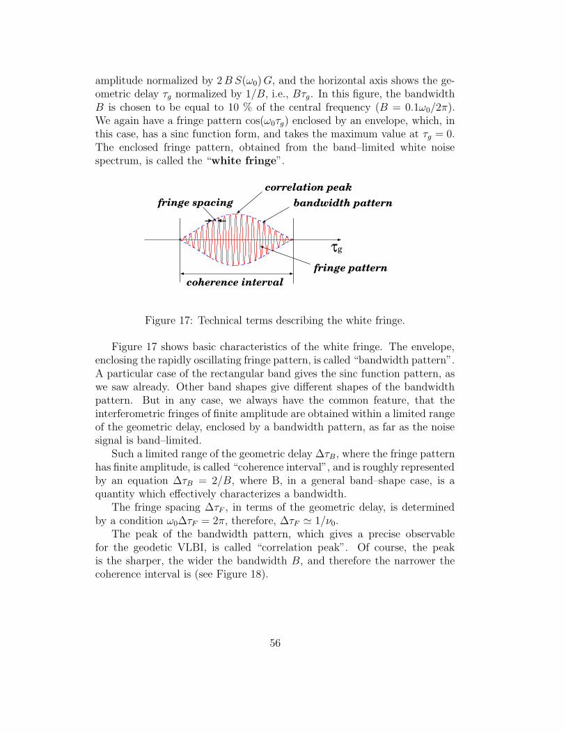
amplitude normalized by 2B S(ω0)G, and the horizontal axis shows the ge-ometric delay τg normalized by 1/B, i.e., Bτg. In this figure, the bandwidthB is chosen to be equal to 10 % of the central frequency (B = 0.1ω0/2π).We again have a fringe pattern cos(ω0τg) enclosed by an envelope, which, inthis case, has a sinc function form, and takes the maximum value at τg = 0.The enclosed fringe pattern, obtained from the band–limited white noisespectrum, is called the “white fringe”.

τg

coherence interval

correlation peakbandwidth pattern

fringe pattern

fringe spacing

Figure 17: Technical terms describing the white fringe.

Figure 17 shows basic characteristics of the white fringe. The envelope,enclosing the rapidly oscillating fringe pattern, is called “bandwidth pattern”.A particular case of the rectangular band gives the sinc function pattern, aswe saw already. Other band shapes give different shapes of the bandwidthpattern. But in any case, we always have the common feature, that theinterferometric fringes of finite amplitude are obtained within a limited rangeof the geometric delay, enclosed by a bandwidth pattern, as far as the noisesignal is band–limited.

Such a limited range of the geometric delay ∆τB, where the fringe patternhas finite amplitude, is called “coherence interval”, and is roughly representedby an equation ∆τB = 2/B, where B, in a general band–shape case, is aquantity which effectively characterizes a bandwidth.

The fringe spacing ∆τF , in terms of the geometric delay, is determinedby a condition ω0∆τF = 2π, therefore, ∆τF ' 1/ν0.

The peak of the bandwidth pattern, which gives a precise observablefor the geodetic VLBI, is called “correlation peak”. Of course, the peakis the sharper, the wider the bandwidth B, and therefore the narrower thecoherence interval is (see Figure 18).

56

-1-0.8-0.6-0.4-0.2

00.20.40.60.8

1

-30 -20 -10 0 10 20 30

norm

aliz

ed c

orre

latio

n

8 GHz white fringe delay in nsec bandwidth 8 MHz

-1-0.8-0.6-0.4-0.2

00.20.40.60.8

1

-30 -20 -10 0 10 20 30

norm

aliz

ed c

orre

latio

n

8 GHz white fringe delay in nsec bandwidth 80 MHz

-1-0.8-0.6-0.4-0.2

00.20.40.60.8

1

-30 -20 -10 0 10 20 30

norm

aliz

ed c

orre

latio

n

8 GHz white fringe delay in nsec bandwidth 800 MHz

Figure 18: White fringes with ceter frequency 8 GHz and various bandwidths:B = 8 MHz (top), B = 80 MHz (middle), and B = 800 MHz (bottom).Horizontal axes show geometric delays covering a range from −30 to 30 nsec.

57

1.3.5 Amplitude and Phase Spectra of the Correlated Signals

Equation (95) shows, that the cross–power spectrum Sv1v2(ω) of the voltagesignals v1(t) and v2(t), received by two antennas, is described through thepower spectrum SEE(ω) of the radio wave coming from a source, and the fre-quency response, assumed rectangular here, of the antenna–receiver system| Q(ω) |2, as:

Sv1v2(ω) = SEE(ω) | Q(ω) |2 e−iωτg .Therefore, if we assume that the real, and even, power spectrum SEE(ω)

0

0 ω

ω

A(ω)

Φ(ω)

∆ω∆ω

ω0ω0-Θ

Figure 19: Amplitude (top) and phase (bottom) spectra of the cross–powerspectrum.

is nearly constant in the receiving frequency band, the amplitude A(ω) andphase Φ(ω) of the cross–power spectrum, which we define as

Sv1v2(ω) = A(ω)e−iΦ(ω), (101)

are expressed as:

A(ω) = SEE(ω) | Q(ω) |2∼= const, (102)

Φ(ω) = ωτg, (103)

within the passband (see Figure 19). Note, that the phase spectrum is ex-pressed by a straight line, crossing the origin and having an inclination tanΘ,which is equal to the geometric delay τg, i.e., tan Θ = τg, in the present sim-ple interferometer model. This is a general feature of the phase spectra ofthe continuum spectrum sources observed by interferometers.

58

1.3.6 Coherence Interval in the Sky

The coherence interval ∆τB = 2/B, in terms of the geometric delay, corre-sponds to a certain angular extent ∆θB in the sky (Figure 20). Following theassumption we made earlier, we consider only a region of the sky which isclose to the direction perpendicular to the baseline of an interferometer withlength D.

∆θB

Figure 20: Coherence interval in the sky.

For a source in the sky, which is separated from a plane perpendicular tothe baseline by an angle θ, the geometric delay τg is equal to

τg =D sin θ

c, and, hence, θ = arcsin

(

c τgD

)

, (104)

where c is the light velocity. Therefore, the angular extent ∆θB is

∆θB = 2 arcsin(

c∆τB2D

)

' c∆τBD

=2c

DB. (105)

The coherence intervals for several values of D and B are listed in Table 1.It is evident from this table that the coherence interval in the sky is fairlynarrow for modern interferometers, especially for VLBI. Therefore, the pas-sive observational mode, which would just “wait for” the passage of a sourcethrough the narrow coherence interval with τg ≈ 0, is extremely ineffectiveand unrealistic, except in the “classical” systems with ∼ 100 m, or shorter,baselines and ∼ a few MHz, or narrower, bandwidths. Consequently, modernradio interferometers are usally equipped with a special mechanism, whichcompensates the delay, by time–shifting one of two received signals, so thatthe signals corresponding to the same wave front are fed to the correlationprocessing simultaneously, as we will see later.

59

bandwidth B 200 kHz 2 MHz 200 MHz 2 GHz

∆τB 10 µsec 1 µsec 10 nsec 1 nsec

∆θB

D = 100 m > 180 > 180 1.7 0.17

D = 10 km 17 1.7 1.′0 6.′′2

D = 1000 km 0.17 1.′0 0.′′62 0.′′062

Table 1: Coherence interval values for various baseline length D and band-width B.

In VLBI, it is very important to know accurate positions of the radiosources and accurate coordinates of the baseline vectors, for successful pre-diction and compensation of the delay, which allow us to detect the fringewithin the quite narrow coherence interval.

1.3.7 Fringe Spacing in the Sky

diurnal motion

∆θfringe spacing

F

Figure 21: Fringe spacing in the sky.

Since the fringe spacing is ∆τF = 1/ν0, in terms of the geometric delay,equation (104) gives the fringe spacing in the sky ∆θF , in the direction nearlyperpendicular to the baseline, as:

∆θF =λ0

D, (106)

where λ0 = c/ν0 is the wave length at the central frequency ν0 of the receivingband (see Figure 21 and Table 2).

60

central frequency ν0 100 MHz 10 GHz 100 GHz

wave length λ0 3 m 3 cm 3 mm

D = 100 m 1.7 1.′0 6.′′2

D = 10 km 1.′0 0.′′62 0.′′062

D = 1000 km 0.′′62 0.′′0062 0.′′00062

Table 2: Fringe spacing values for various baseline length D and centralfrequency ν0.

The angular resolution of an interferometer is usually expressed by equa-tion (106), since the resolution is essentially determined by the fringe spacing.

Since every radio source diurnally moves across the dense fringe patternin the sky with the very short fringe spacing, the phase of the cosine termω0τg in equation (100) changes very rapidly. Therefore, the correlator outputof the signals of our simple interferometer must oscillate also very rapidly.This would make mostly impossible to integrate the multiplier output fora duration of time, which is long enough to detect the white fringe with asufficiently high signal–to–noise ratio, since any simple time averaging (inte-gration) of an oscillating signal results in almost zero signal only (Figure 22).Therefore, modern radio interferometers are usually equipped with a specialmechanism to compensate (or stop) the rapid phase change, as we will seelater.

T

t0

Figure 22: What will come out, if we integrate (time average) this?

2 A Realistic Radio Interferometer

The simple interferometer, which we discussed in the previous section, washelpful for understanding one of the most important concepts for radio inter-

61

ferometry, the white fringe. Nevertheless, the simple model is far from realmodern radio interferometers in following aspects.

First, radio sources are not mere points. They usually show structures,or intensity distributions, in the sky. One of the main purposes of the VLBI,or radio interferometry in general, is to obtain images of the radio sourcestructures. But if the source is not point–like, the delayed voltage modelin equation (86), which was described through a single geometric delay ofa point source, must be no longer valid. Moreover, if the source structuresare extended, we have to take into account the beam patterns of elementantennas, as well.

LocalOscillator

Beam Pattern 2

Beam Pattern 1

Receiver 2Receiver 1

D

s0

cτg =

D s

0.

IntegratorMultiplier

τi

Mixer

InstrumentalDelay

Extended Source

Source structureand different antenna-receivercharacteristics

Frequencyconversion

Compensation ofdelay and phasechange

Correlator

Figure 23: A realistic interferometer.

Second, the antennas and receiving systems in a radio interferometer arenot identical, in general. Therefore, the beam patterns and the frequencyresponses of the antenna–receiver systems may differ from each other, unlikein the simple interferometer model.

Third, receiving systems in modern interferometers are usually based onthe superheterodyne design, and correlation processings are performed for IF(intermediate frequency) signals after the frequency conversion, but not forRF signals, as assumed in the simple interferometer model.

62

Finally, we have to introduce the special mechanisms in order to com-pensate the geometric delay and the rapid phase change in the correlatoroutput, as we noted in the last two paragraphs of the previous section. Thisshould be done so that we can always observe a radio source whenever it isabove the horizon, but not just within a very short duration of time, whilethe source happenes to pass the very narrow coherence interval.

However, we still neglect, for a while, atmospheric and instrumental de-lays, other than the geometric delay. Also, we ignore, as before, any con-tribution of the system noise, in order to concentrate our attention to thecharacteristics of the correlated radio source signals only.

Figure 23 illustrates a “more realistic” 2–element interferometer. In thefollowing subsections, we will examine effects of the source structure anddiffferent antenna–receiver characteristics, the frequency conversion, and thecompensation of the delay and the phase change, in turn.

2.1 Source Structure, Visibility and Intensity

2.1.1 Source Coherence Function

How the correlator output of an interferometer is related to the intensity (orbrightness) distribution of a radio source in the sky?

In order to answer to this question, we must consider how the electro-magnetic field from a source, which is received and converted to the voltagesignal by each antenna of the interferometer, is related to the intensity dis-tribution of the source. For this purpose, we first address ourselves to aproblem regarding properties of radio waves from an extended radio source,namely, whether radio waves coming from different points of a radio sourceare mutually correlated, or not.

Let us choose a certain direction in the source (for example, the directionof the maximum intensity), which is denoted by a unit vector s0, as a refer-ence direction. Then a unit vector s, pointing towards an arbitrary directionin the source, may be expressed as s = s0 + σ, and we can use the “offsetvector from the reference direction” σ ≡ s− s0, as a vector, which is almostconfined in the celestial sphere and indicates the direction s. See Figure 24for the geometry.

As a quantity representing the electromagnetic wave from the source, weagain choose a single polarization component of the electric field intensityE(t), to be received by the antennas. Since the source is now extended, wedenote a component of the electric field intensity, which comes from a unitsolid angle around a direction σ, as e(σ, t). Then the incident electric field

63

s0

s’

sσ ’

e(σ ’,t’)

e(σ ,t)

σ

Figure 24: Radio waves coming from different directions in a radio source.

from the whole source E(t) is expressed through e(σ, t) as

E(t) =∫

source

e(σ, t)dΩ, (107)

where dΩ is an infinitesimal solid angle element. Now, let us consider across–correlation of electric field components e(σ, t) and e(σ ′, t′), comingfrom different directions σ and σ

′, and taken at different times t and t′:

〈e(σ, t) e(σ′, t′)〉,(see Figure 24).

Assuming again that e(σ, t) and e(σ′, t′) are jointly stationary randomprocesses, we express the cross–correlation as a function of time differenceτ = t− t′:

γ(σ,σ′, τ) = 〈e(σ, t) e(σ′, t′)〉. (108)

This function γ(σ,σ′, τ) is called “source coherence function”.Using this source coherence function, we define a cross–correlation coef-

ficient , which is called “normalized source coherence function”:

γN(σ,σ′, τ) =γ(σ,σ′, τ)

√

γ(σ,σ, 0)γ(σ′,σ′, 0), (109)

(here, we assume that the expectation of the electric field 〈e(σ, t)〉 = 0, and,therefore, the cross–correlation is equal to the cross–covariance). Accordingto the general property of the cross–correlation coefficient, the normalizedsource coherence function always satisfies

0 ≤| γN(σ,σ′, τ) |≤ 1.

64

Now we use following definitions.

1. Radio waves from different directions σ and σ′ are called “completely

coherent” if | γN(σ,σ′, τ) |= 1 for any τ , and “completely incoherent”if | γN(σ,σ′, τ) |= 0 for any τ .

2. A radio source is called “coherent” if radio waves from any differentdirections σ and σ

′ in the source are completely coherent, and “inco-herent” if the waves are completely incoherent. In all other cases, theradio source is called “partially coherent”.

If someone puts many transmission antennas in a town, and broadcasts aTV programm, then any “poor–reception–level” problem would simply dis-appear. Instead, however, we would suffer from a serious “ghost” problem,since TV signals from different antennas are mutually coherent. The “ghost”images would drastically change when we slightly shift or rotate our TV re-ception antenna to an extent, comparable with the wavelength of the TVsignal. Therefore, it would even become difficult to know directions of trans-mission antennas in the easy way, by just rotating the reception antennaand watching the screen. But if the TV broadcasting is turned off, and onlyincoherent (independent) noises are emitted from transmission antennas, itwould get much easier to know their directions.

Fortunately, most of actual astronomical radio sources are known to beincoherent, and, therefore, can be imaged relatively simply. This is becauseradio waves emitted from the source regions are just mutually independentnoises generated by random microscopic processes occuring there. Therefore,in following discussions, we assume that radio sources are incoherent.

Then, the source coherence function must be expressed as

γ(σ,σ′, τ) = γ(σ, τ)δ(σ − σ′), (110)

since radio waves from directions σ and σ′ are correlated only when σ = σ

′.The function γ(σ, τ), defined by equation (110), is called “self–coherencefunction”.

2.1.2 Power of Electric Field Incident from a Certain Direction

The autocorrelation of the electric field E(t) is expressed through the self–coherence function as:

〈E(t)E(t′)〉 =∫ ∫

source

〈e(σ, t)e(σ′, t′)〉dΩdΩ′

=∫ ∫

source

γ(σ, τ)δ(σ − σ′)dΩdΩ′ =

∫

source

γ(σ, τ)dΩ. (111)

65

Therefore, we obtain, for a mean square value of the electric field E(t),

〈E(t)2〉 =∫

source

γ(σ, 0)dΩ, (112)

which implies that γ(σ, 0) is a “density per solid angle” of the mean squareelectric field in the direction of σ.

Consequently, if we consider a total electric field vector E(t), which comesfrom a small solid angle element ∆Ω towards a direction σ, and includes bothof the two independent polarization components, then its mean square value(or power) is related to the self–coherence function at τ = 0 as:

1

2〈| E(σ) |2〉 = γ(σ, 0) ∆Ω, (113)

where the coefficient 1 / 2 corresponds to the fact that γ(σ, 0) includes onlya single polarization component of the electric field.

2.1.3 Poynting Flux

Now we proceed to the relation between the incident electric field and thesource intensity (or brightness) distribution. First, we consider a quantity,characterizing the incident electromagnetic wave, which we call “Poyntingflux through a cross section”.

Let us consider the Poynting vector S(σ) of an electromagnetic wave,which comes from the same small solid angle element ∆Ω towards the di-rection σ, as in equation (113). Let ∆Ω be small enough that the wave iswell approximated by a superposition of monochromatic plane waves prop-agating along the same direction, with individual frequencies contained in afinite bandwidth of the incident wave.

As we saw in Chapter 2, the Poynting vector Sm(σ) of a monochromaticplane wave is given, in terms of the corresponding electric field intensityEm(σ), by an equation:

Sm(σ) =1

Zn | Em(σ) |2, (114)

where Z is the intrinsic impedance of the medium, and n = −s = −(s0 +σ)is a unit vector along a direction of the wave propagation.

The term | Em(σ) |2, in equation (114), corresponds to a power of theelectric field, contained within an infinitesimally narrow frequency band ofa monochromatic plane wave. Such a power is equal to the power spectrumat the frequency of the band, multiplied by the bandwidth, as we discussed

66

in subsection 1.2.8. On the other hand, the power | E(σ) |2, contained in afinite bandwidth, is simply equal to the integral of the power spectrum overthe bandwidth. Hence, we obtain the power | E(σ) |2, by just summing upall monochromatic plane wave components | Em(σ) |2 over the bandwidth:

| E(σ) |2=∑

| Em(σ) |2 .Meanwhile, the Poynting vector S(σ), with the finite bandwidth, is a

vector sum of all monochromatic plane wave components Sm(σ):

S(σ) =∑

Sm(σ).

Therefore, an equation, with the same form as the one in the monochro-matic plane wave case, given in equation (114), holds also for the Poyntingvector S(σ) and the power of the electric field | E(σ) |2, having the finitebandwidth:

S(σ) =1

Zn | E(σ) |2 . (115)

Let us now consider “Poynting flux through a cross section”, or simply“Poynting flux”, which we define as equal to the energy of the electromagneticwave passing through a certain cross section of unit area, per unit duration

nN

∆Ωσ

s 0

S( )σθ

s

Figure 25: Poynting flux through a cross section.

of time. If we denote a unit vector normal to the cross section as N , thePoynting flux of the wave coming from the direction σ is given by a projectionof the Poynting vector on the direction N :

S(σ) · N =1

Z| E(σ) |2 cos θ, (116)

67

where θ is an angle between the normal unit vector N of the cross sectionand the direction n of the wave propagation (see Figure 25).

Now we consider the Poynting flux S of the wave not only from a smallsolid angle towards σ, but from the all source area:

S =∑

n

S(σn) · N =1

Z

∑

n

| E(σn) |2 cos θn, (117)

where∑

n

means a summation of all small solid angle elements towards direc-

tions σ1,σ2, · · · ,σn, · · ·, covering the whole source area, and θn is an anglebetween the normal to the cross section N and the direction of propagationnn = −(s0 + σn).

Combining this equation with equation (113), we obtain an equation re-lating a mean Poynting flux to the self–coherence function:

〈S〉 =1

Z

∑

n

〈| E(σn) |2〉 cos θn =2

Z

∑

n

γ(σn, 0) cos θn∆Ωn, (118)

where ∆Ωn is a small solid angle element towards a direction σn. If we replacethe summation, with respect to the small solid angles, by an integration, therelation between the mean Poyinting flux 〈S〉 and the self–coherence functionγ(σ, τ) is given by:

〈S〉 =2

Z

∫

source

γ(σ, 0) cos θdΩ. (119)

If we further introduce the Fourier transform γ(σ, ω) of the self–coherencefunction γ(σ, τ) in the angular frequency ω space, i.e., γ(σ, τ) ⇔ γ(σ, ω):

γ(σ, ω) =

∞∫

−∞

γ(σ, τ) e−iωτdτ, (120)

γ(σ, τ) =1

2π

∞∫

−∞

γ(σ, ω) eiωτdω,

then, we have

γ(σ, 0) =

∞∫

−∞

γ(σ, ω) dν,

where ν is a frequency corresponding to the angular frequency ω, i.e., ν =ω/(2π). Since Fourier transform of a real function is an even function of thefrequency, γ(σ, 0) is also given as:

γ(σ, 0) = 2

∞∫

0

γ(σ, ω) dν. (121)

68

Therefore, the mean Poynting flux in equation (119) is now given as:

〈S〉 =4

Z

∞∫

0

∫

source

γ(σ, ω) cos θ dΩ dν. (122)

2.1.4 Electric Field and Radio Source Intensity — Electromag-netics and Astronomy

As we saw in Chapter 1, results of radio astronomical observations are char-acterized by a number of quantities, such as, “intensity” Iν, “spectral fluxdensity” Sν, and “power flux density” S. These quantities are phenomeno-logically defined in astronomy. For example, the intensity is defined as “thequantity of radiation energy incoming from a certain direction in the sky,per unit solid angle, per unit time, per unit area perpendicular to this di-rection, and per unit frequency bandwidth with center frequency ν”. As wesee, no electromagnetic quantity, such as electric field intensity E, or volt-age v, appears in such a phenomenological definition. Therefore, we mustprecisely define a certain relationship between the electromagnetic and ra-dioastronomical quantities, in order to describe radioastronomical results interms of the electromagnetic quantities, which we actually measure in ourradio telescopes.

Such a relationship was defined by IEEE (Institute of Electrical and Elec-tronics Engineers) in 1977. According to the definition, the power flux densityin astronomy is equal to the time average of the Poynting vector in electro-magnetics.

The power flux density S is defined in astronomy as “the quantity ofradiation energy, over the whole frequency range, incoming through a crosssection of unit area, per unit time”. This quantity is related to the spectralflux density Sν , and to the intensity Iν as:

S =

∞∫

0

Sν dν =

∞∫

0

∫

source

Iν(σ) cos θ dΩ dν, (123)

because the spectral flux density is defined as “the quantity of radiationenergy incoming through a cross section of unit area, per unit frequencybandwidth, and per unit time”, and the intensity is defined as we saw above.

Since the power flux density is given with respect to a certain cross sectionof unit area, we interpret the “Poynting vector”, in the IEEE definition as aPoynting flux, through the cross section.

Then, the definition of IEEE (1977) requires that the mean Poynting flux〈S〉 must be equal to the power flux density S:

〈S〉 = S, (124)

69

since, in view of the Ergodicity, the time average must be equal to the statis-tical mean, provided that the averaging time is sufficiently long. Therefore,from equations (122) and (123), we have

∞∫

0

∫

source

Iν(σ) cos θ dΩ dν =4

Z

∞∫

0

∫

source

γ(σ, ω) cos θ dΩ dν. (125)

Generally speaking, equal integrals do not necessarily mean equal inte-grands, of course. However, in our case of the stationary random signal froman incoherent source, we can equate integrands of the both sides of equation(125). In fact, the total power of the electric field intensity is simply equalto a sum of contributions from all elements in frequency bands and spa-tial solid angles. To make this point more evident, let us imagine a virtualsource which emits radiation only in limited frequency and spatial solid–angleranges of the actual radio source. The average Poynting flux and the powerflux density from this virtual source are equal to those of the actual sourcein the respective frequency and solid–angle ranges. They must be expressedthrough the self–coherence function and the intensity, just in the same formsas those given in equations (122) and (123), but with limited frequency andsolid–angle ranges of the integrations. Since the definition of IEEE (1977)requires their equality, for this virtual source as well, equation (125) musthold for arbitrary frequency range ∆ν and arbitrary spatial solid–angle range∆Ω, i.e.,

∫

∆ν

∫

∆Ω

Iν(σ) cos θ dΩ dν =4

Z

∫

∆ν

∫

∆Ω

γ(σ, ω) cos θ dΩ dν,

which implies that the integrands must be equal to each other. Therefore,we have

Iν(σ) =4

Zγ(σ, ω). (126)

This is a relation between the source intensity distribution and the spectrumof the self–coherence funtion, which is the density per solid angle of the powerof the incident electric field, as we saw before. Thus, we succeeded to relatethe source intensity distribution in astronomy to the incident electric field inelectromagnetics.

2.1.5 Field of View of a Radio Telescope

The incident electric field is converted to the voltage in a radio telescope an-tenna, and this voltage is actually processed in our detecting devices (square–law detectors, or correlators). Then, how can we relate the received voltage

70

v(t) to the source intensity distribution? Here, we must take into accountthat an antenna collects electric fields, coming from different directions in aradio source, weighting them according to its beam pattern, specifically thevoltage reception pattern, which we saw in Chapter 2. This “field of view”effect must be properly corrected for, prior to infering the source intensitydistribution from detected signals (Figure 26).

s0

s’

s σσ ’

e(σ ’,t’)

e(σ ,t)

Voltage reception pattern

v(t)

Figure 26: Voltage reception pattern.

In order to consider this problem, it is convenient to move from the timedomain to the frequency domain, since, as we saw in Chapter 2, the beampattern of an antenna is a function of frequency (the beam width is roughlyproportional to ν−1).

Let us consider Fourier transforms e(σ, ω) and v(ω) of the single polar-ization component of the electric field intensity e(σ, t), coming from a unitsolid angle of direction σ, and the received voltage v(t), respectively.

e(σ, ω) =

∞∫

−∞

e(σ, t)e−iωtdt, (127)

v(ω) =

∞∫

−∞

v(t)e−iωtdt. (128)

Since we assume that the electric field intensity e(σ, t) and the receivedvoltage v(t) are stationary random processes, these are examples of the

71

Fourier transforms of stationary random processes, which we discussed insubsection 1.2.9.

Without being involved in details of electromagnetics on wave reception,we just assume that the received voltage at a certain frequency is proportionalto incident electric field intensity collected by the antenna beam at the samefrequency. Then, we introduce the voltage reception pattern Q(σ, ω) as afunction relating v(ω) and e(σ, ω) through an equation:

v(ω) =∫

source

e(σ, ω)Q(σ, ω) dΩ. (129)

Note that the voltage reception pattern thus defined has a dimension oflength (unit of voltage is V and unit of electric field intensity is Vm−1).The voltage reception pattern is, in general, a complex quantity, since thereception process might be associated with some energy dissipation.

2.1.6 Power Pattern of a Receiving Antenna

Let us now establish a relationship between the voltage reception pattern,as defined in equation (129), and the power pattern of a receiving antenna,which we empirically introduced in Chapter 2. Although this is a topicrelated to a single–dish radio telescope, following discussions will serve asuseful preparations for further considerations of interferometers.

If we denote a resistance in the circuit of the receiving system as R, thenaveraged power W and received voltage v(t) are related to each other by anequation:

W =〈v2〉R. (130)

Introducing an autocorrelation Rvv(τ):

Rvv(τ) = 〈v(t) v(t′)〉, (131)

and power spectrum Svv(ω):

Svv(ω) =

∞∫

−∞

Rvv(τ)e−iωτdτ, (132)

Rvv(τ) =1

2π

∞∫

−∞

Svv(ω)eiωτdω, (133)

of the received voltage v(t), we reexpress equation (130) as

W =Rvv(0)

R=

2

R

∞∫

0

Svv(ω) dν. (134)

72

Hence, the power per unit frequency bandwidth Wν, which satisfies

W =

∞∫

0

Wν dν,

is given by

Wν =2

RSvv(ω). (135)

Now, let us express the power spectrum Svv(ω) in terms of the incidentelectric field intensity. For this purpose, we first calculate the autocorrelationof the Fourier transform v(ω) of the received voltage v(t). In view of equation(129), we have

〈v(ω)v∗(ω′)〉 =∫ ∫

source

〈e(σ, ω)e∗(σ′, ω′)〉Q(σ, ω)Q∗(σ′, ω′)dΩdΩ′. (136)

Here, the cross–correlation 〈e(σ, ω)e∗(σ′, ω′)〉 of the Fourier transforms ofthe incident electric field intensities, must be in a form:

〈e(σ, ω)e∗(σ′, ω′)〉 = 2πγ(σ, σ′, ω) δ(ω − ω′), (137)

since we assume them as stationary random processes, which satisfy equation(83). In the right hand side of equation (137), we introduced a cross–powerspectrum γ(σ, σ

′, ω) of the electric field intensities, which is the Fouriertransform of the source coherence function γ(σ, σ

′, τ), as defined in equation(108).

Since we assume an incoherent source, the source coherence function isexpressed through the self–coherence function γ(σ, τ), as given in equation(110). Therefore, the cross–power spectrum must be given as:

γ(σ, σ′, ω) = γ(σ, ω) δ(σ − σ

′). (138)

Hence, equation (137) is rewritten as:

〈e(σ, ω)e∗(σ′, ω′)〉 = 2πγ(σ, ω)δ(σ − σ′)δ(ω − ω′). (139)

Inserting this equation to equation (136), we obtain

〈v(ω)v∗(ω′)〉 = 2π

∫

source

γ(σ, ω) | Q(σ, ω) |2 dΩ

δ(ω − ω′). (140)

Now, on the other hand, the autocorrelation 〈v(ω)v∗(ω′)〉 must also beexpressed through the power spectrum Svv(ω) of the voltage as:

〈v(ω)v∗(ω′)〉 = 2πSvv(ω)δ(ω − ω′), (141)

73

in view of equation (82), which is a general property of Fourier transformsof the stationary random processes. Thus, from equations (140) and (141),we obtain

Svv(ω) =∫

source

γ(σ, ω) | Q(σ, ω) |2 dΩ, (142)

or, taking into account equations (126) and (135),

Wν =Z

2R

∫

source

Iν(σ) | Q(σ, ω) |2 dΩ. (143)

Equation (143) must be equivalent to the equation

Wν =1

2Ae

∫

source

Iν(σ)Pn(σ)dΩ, (144)

which we introduced in Chapter 2, in order to express the power per unitbandwidth received by an antenna with a normalized power pattern Pn(σ)and an effective aperture Ae. Noting again, that we can select arbitrary solidangle as the source range, we can equate integrands of equations (143) and(144), to obtain

| Q(σ, ω) |2= R

ZAePn(σ). (145)

This is the relation between the voltage reception pattern and the normalizedpower pattern.

From equations (126) and (145), the power spectrum of the received volt-age in equation (142) is now given as:

Svv(ω) =1

4Ae

∫

source

Iν(σ)Pn(σ) dΩ. (146)

2.1.7 New Dimensions of Voltage and Electric Field

For further discussions, it is convenient to redefine the volatage and theelectric field intensity as

v(t)√R

−→ v(t),

e(σ, t)√Z

−→ e(σ, t), (147)

to eliminate constant coefficients of the resistance R and the intrinsic impedanceZ, which may cause rather complicated appearances of our equations. Then,dimensions of the voltage and the electric field intensity change to

74

• voltage v [electric power]1/2 (W1/2)

• electric field intensity e [power flux density]1/2 (W1/2 m−1),

and we have

Svv(ω)

R−→ Svv(ω),

γ(σ, ω)

Z−→ γ(σ, ω), (148)

for the power spectra of the voltage and the electric field intensity.Let us further redefine the voltage reception pattern as

√

Z

RQ(σ, ω) −→ Q(σ, ω). (149)

Then, the voltage — field relation remain in the same form as equation (129):

v(ω) =∫

source

e(σ, ω)Q(σ, ω)dΩ,

and we obtain simple expressions:

Wν = 2Svv(ω),

Iν(σ) = 4γ(σ, ω),

AePn(σ) = | Q(σ, ω) |2,(150)

for the power per unit bandwidth, the source intensity, and the normalizedpower pattern.

2.1.8 How Does A Radio Interferometer View the Universe?

A radio interferometer can be regarded as an instrument which yields a cross–correlation or a cross–power spectrum of voltages received at antennas. Weconsider now the cross–correlation and cross–power spectrum of the voltages“just received”, which we will call hereafter “received voltages”. Althoughactual correlation processing is performed for voltages after frequency conver-sion and compensation of the delay and the phase change, present discussionis quite meaningful, since the final results are described through the spectrumof the received voltages, as we will see later.

Let us again consider a two–element interferometer, such as shown inFigure 27. Let a baseline vector D be drawn from antenna 1 to antenna 2,

75

D

s = s0 + σ

τ g

s0

σ

1 2

(σ)

Figure 27: Geometry of a two element radio interferometer.

and let a unit vector s = s0 + σ point towards a certain direction within aradio source, where s0 shows a reference direction of the source, as before.

Then, the geometric delay, between arrivals of the same wave front fromthe direction s at two antennas, is given by

τg(σ) =D · sc

= τg0 +D · σc

, (151)

where c is the light velocity, τg0 ≡D · s0

cis a geometric delay of the wave

coming from the reference direction s0, and we use the offset vector σ = s−s0

for denoting the direction s within the source. For simplicity, we ignore hereany atmospheric or instrumental delay effect, other than the geometric delay.

Now, the electric field intensities e1(σ, t) and e2(σ, t), with a single po-larization component, which arrive at two antennas at a certain time t fromthe same direction σ, are described through a common incident field intensitye(σ, t), representing the same wave front, as

e1(σ, t) = e(σ, t− τg(σ)),

e2(σ, t) = e(σ, t).(152)

Therefore, their Fourier transforms e1(σ, ω) and e2(σ, ω) are given by

e1(σ, ω) = e(σ, ω)e−iωτg(σ),

e2(σ, ω) = e(σ, ω),(153)

where e(σ, ω) is the Fourier transform of e(σ, t). We used equation (68) ofthe shift theorem, in deriving the upper equation of equation (153).

76

These electric field intensities are converted to voltages at the two anten-nas:

v1(ω) =∫

source

e1(σ, ω)Q1(σ, ω)dΩ,

v2(ω) =∫

source

e2(σ, ω)Q2(σ, ω)dΩ, (154)

according to equation (129).Therefore, their cross–correlation is given by

〈v1(ω) v∗2(ω′)〉 =

∫ ∫

source

〈e1(σ, ω)e∗2(σ′, ω′)〉Q1(σ, ω)Q∗

2(σ′, ω′)dΩdΩ′.

(155)In view of equation (153), we can here express the electric field intensities attwo antennas through the common incident electric field intensity e(σ, ω):

〈e1(σ, ω)e∗2(σ′, ω′)〉 = 〈e(σ, ω)e∗(σ′, ω′)〉e−iωτg(σ). (156)

Since the electric field is regarded as a stationary random process, and theradio source is assumed to be incoherent, we have equation (139) again for〈e(σ, ω)e∗(σ′, ω′)〉:

〈e(σ, ω)e∗(σ′, ω′)〉 = 2πγ(σ, ω) δ(σ − σ′) δ(ω − ω′).

Therefore, the cross–correlation of the Fourier transforms of the receivedvoltages 〈v1(ω) v∗2(ω

′)〉 in equation (155) are now given by

〈v1(ω) v∗2(ω′)〉 = 2π

∫

source

γ(σ, ω)Q1(σ, ω)Q∗2(σ, ω)e−iωτg(σ) dΩ

δ(ω − ω′).

(157)On the other hand, since the voltages received at two antennas are jointly

stationary random processes (they originate from the same incident wavefront), the cross–correlation of their Fourier transforms and their cross–powerspectrum are related to each other by the general formula of equation (83):

〈v1(ω) v∗2(ω′)〉 = 2πSv1v2(ω) δ(ω − ω′). (158)

From equations (157) and (158), we obtain

Sv1v2(ω) =∫

source

γ(σ, ω)Q1(σ, ω)Q∗2(σ, ω) e−iωτg(σ) dΩ. (159)

77

Now, equation (150) shows that the Fourier transform γ(σ, ω) of the self–coherence function and the source intensity Iν(σ) are related to each otheras

γ(σ, ω) =1

4Iν(σ).

Furthermore, equation (150) also shows that the voltage reception patternQ(σ, ω) and the normalized power pattern Pn(σ) of an antenna are relatedto each other as

Ae Pn(σ) =| Q(σ, ω) |2,where Ae is the effective aperture of the antenna. So, let us introduce herean analog of this equation in an interferometer case:

A0AN(σ) = Q1(σ, ω)Q∗2(σ, ω), (160)

where A0 is a geometrical mean of effective apertures of two antennas:

A0 =√

Ae1 Ae2 , (161)

and AN (σ) is called “normalized power pattern of an interferometer”. Whenthe two voltage reception patterns Q1 and Q2 are real quantities (i.e., there isno phase change associated with the field → voltage conversion), or they haveequal phases, AN (σ) is described through the normalized power patterns Pn1

and Pn2 of the respective single–dish antennas as:

AN(σ) =√

Pn1(σ)Pn2(σ). (162)

Taking into account equations (150), (151) and (160), and denoting

ωD · σc

= 2πDλ · σ, (163)

where Dλ = D/λ is the baseline vector normalized by the wavelength λ =2πc/ω, we rewrite equation (159) in a form:

Sv1v2(ω) =1

4A0 e

−iωτg0

∫

source

AN(σ) Iν(σ) e−i2πDλ·σdΩ. (164)

This equation gives a relationship between the cross–power spectrum of thereceived voltages and the intensity distribution of the radio source. This isan interferometer analog of the power–spectrum — intensity relationship ina single dish antenna, given in equation (146):

Svv(ω) =1

4Ae

∫

source

Pn(σ) Iν(σ) dΩ.

78

In closing this subsection, it is worthwhile to notice an approximationmade in our treatment of the geometric delay. In deriving equation (153)from equation (152), we implicitly assumed that the geometric delay τg isconstant in time, though, of course, the geometric delay must change in timedue to the diurnal motion of the Earth. Such a quasi–static approach is goodenough for our present purpose to understand basic features of radio interfer-ometry, and we will continue to follow this approach hereafter. However, itshould be noted that the quasi–static approach does not allow us to properlytake account of some observable effects, such as Doppler shift in amplitude ofcross–power spectrum of a radio source due to the Earth’s rotation. Conse-quently, formulae we provide here lack these effects. More complete accountof this problem will require some modification in our assumption of the sta-tionary random natutre of the received signals.

2.1.9 Complex Visibility

The cross–power spectrum of the received voltages Sv1v2(ω) is an observablequantity, which can be derived from the correlator output, as we will seein more detail, later. Equation (164) shows that the cross–power spectrumis a product of three terms: the geometric mean of the effective aperturesA0, the exponential term which depends on the geometric delay τg0 at thereference direction s0 of the observed source, and an integral over the solidangle of the source. The exponential term stands for the fringe pattern,which we discussed in section 1.3. Therefore, the integral term figures as acomplex coefficient of the fringe pattern. We can derive this integral termfrom the observed cross–power spectrum, since A0 is almost constant and canbe estimated independently, and the fringe pattern is known, as far as weknow the source direction and the baseline vector with sufficient accuracies.

We call the integral, or the complex coefficient of the fringe pattern,“complex visibility”, “fringe visibility”, or just “visibility”, and denote it asV(ω):

V(ω) =∮

AN (σ) Iν(σ) e−i2πDλ·σ dΩ. (165)

Here, we expanded the range of integration from the source region to thewhole sky, since we expect Iν(σ) = 0 outside the source region, and radiosources far from the antenna beam direction do not contribute to the integral,simply because AN (σ) = 0 for those sources.

Equation (165) shows the relationship between the complex visibility andthe intensity distribution of the radio source. Amplitude | V(ω) | and phaseΦv of the complex visibility:

V(ω) =| V(ω) | eiΦv(ω), (166)

79

are called “visibility amplitude” and “visibility phase”, respectively.The complex visibility as shown in equation (165) has a dimension of the

flux density (w m−2 Hz−1). In fact, the complex visibility can be regarded asan analog of the effective flux density Sν received by a single–dish antenna:

Sν =∮

Pn(σ) Iν(σ) dΩ, (167)

which we introduced in Chapter 2. Thus, the visibility amplitude is alsocalled as “correlated flux density”.

Although equations (165) and (167) show similar forms, and the similarityclearly comes from a common physical nature of the complex visibility andthe effective flux density, there is a big difference between these quantities,as well. While angular resolution of a single–dish observation is determinedby the normalized power pattern of an antenna Pn(σ) in equation (167),angular resolution of an interferometer observation is essentially determined

by e−i2πDλ·σ term in equation (165), which represents the fringe patternof the interferometer, but not by the normalized power patterns of elementantennas figuring in AN(σ). In this sense, the complex visibility could beregarded as the “intensity collected by a fringe pattern”, in contrast to theeffective flux density, which is the “intensity collected by an antenna beam”.

The cross–power spectrum of the received voltages is given through thecomplex visibility as:

Sv1v2(ω) =1

4A0 e

−iωτg0 V(ω). (168)

This is an analog of the single–dish relation:

Svv(ω) =1

2Wν =

1

4Ae Sν , (169)

where Ae is the effective aperture of the antenna, and Wν is the receivedpower per unit frequency, as before.

The complex visibility is an important quantity of the interferometry forinfering the structure, or “image”, of the observed source, as we will discusslater.

2.2 Frequency Conversion in Radio Interferometers

It has been technically impossible to cross–correlate received voltage signalsat RF frequencies higher than ∼ 1 GHz. Therefore, in modern radio inter-ferometers, the received RF signals have been frequency–converted to lowerIF frequencies, before the correlation processing (Figure 28).

80

So, let us now consider how cross–power spectra SvI1vI2(ω) of IF sig-

nals are related to the cross–power spectra Sv1v2(ω) of RF signals, which wehave so far discussed (see, for example, equation (168)). It is interesting toemamine, in particular, if the condition of stationary randomness of the RF

v1(t) v2(t)hR2hR1 SvR1vR2(ω)

Sv1v2(ω)

RF Filter(LNA + BPF)

RF signalvR1(t) vR2(t) LocalOscillator

Mixer

hI1 hI2

vI2(t)vI1(t)

SvI1vI2(ω) IF Filter(IF Amp + BPF)

IF signal

to correlator to correlator

Received signal

Figure 28: How the cross–power spectrum SvI1vI2(ω) of IF signals are related

to the cross-power spectrum Sv1v2(ω) of received signals?

signals are conserved after the frequency conversion, where the RF signals are“mixed” (multiplied and then band–pass filtered) with sinusoidal referencesignals provided from LOs (local oscillators).

2.2.1 Response of RF Filters

The RF signals are usually amplified and band–pass filtered, before the fre-quency conversion, in cm– and long mm–wave observations. Therefore, wefirst take into account, in a general form, responses of the RF filters, whichare usually composed of LNAs (low noise amplifiers) and BPFs (band–passfilters). In cases, when first stage devices in receiving systems are mixers,such as SIS mixers used in short mm–wave observations, this step must besimply ommited.

81

Let us consider that an RF filter is a linear system, whose input is thereceived voltage v(t), output is a voltage denoted as vR(t), and filter responseis described by a real impulse response hR(t).

Then, we havevR(t) = v(t) ∗ hR(t). (170)

This means, in view of the convolution theorem given in equation (66), thatFourier transforms v(ω) and vR(ω) of the stationary random processes v(t)and vR(t), respectively, and system function HR(ω) of the impulse responsehR(t):

v(t) ⇔ v(ω), vR(t) ⇔ vR(ω), hR(t) ⇔ HR(ω), (171)

satisfyvR(ω) = v(ω)HR(ω). (172)

The system function HR(ω) here stands for effects of the LNA gain andband–pass characteristics of the BPF.

Thus, for Fourier transforms of input voltage signals v1(t) and v2(t), re-ceived at two antennas, and output voltages vR1(t) and vR2(t) of RF filters,with impulse responses hR1(t) and hR2(t), respectively,

v1(t) ⇔ v1(ω), vR1(t) ⇔ vR1(ω), hR1(t) ⇔ HR1(ω),

v2(t) ⇔ v2(ω), vR2(t) ⇔ vR2(ω), hR2(t) ⇔ HR2(ω), (173)

we have

vR1(ω) = v1(ω)HR1(ω),

vR2(ω) = v2(ω)HR2(ω). (174)

Hence, cross–correlation of vR1(ω) and vR2(ω) is givn by

〈vR1(ω) v∗R2(ω′)〉 = 〈v1(ω) v∗2(ω

′)〉HR1(ω)H∗R2(ω

′). (175)

Now, in view of the general properties of cross–correlations of Fouriertransforms of stationary random processes, given in equation (83), we have

〈vR1(ω) v∗R2(ω′)〉 = 2π SvR1vR2

(ω) δ(ω − ω′),

〈v1(ω) v∗2(ω′)〉 = 2π Sv1v2(ω) δ(ω − ω′), (176)

where Sv1v2(ω) and SvR1vR2(ω) are cross–power spectra of input voltages v1(t)

and v2(t), and output voltages vR1(t) and vR2(t), respectively, of the RFfilters. Consequently, equation (175) yields a relation:

SvR1vR2(ω) = Sv1v2(ω)HR1(ω)H∗

R2(ω), (177)

between the cross–power spectra of input and output signals of the RF filters(see Figure 28). Note that the cross–power spectrum of the received voltagesSv1v2(ω) is related to the complex visibility of an observed source in equation(168).

82

2.2.2 Fourier Transform of IF Voltage Signal

Let us now proceed to the problem of the frequency conversion.Actual frequency conversion is often performed through several steps, by

sequentially shifting a spectral range, which contains observed data, fromhigher frequencies to lower frequencies, in turn. However, we assume herea simplified scheme, where single frequency conversion units down–convertRF signals to final IF signals, at once. Basically, multi–step conversion isequivalent to a single–step conversion, as long as the total frequency shiftsand total band–pass characteristics are the same in both schemes. Therefore,our simplified assumption will not lower generality of following discussions.

Mixer2 cos(ωLOt + φLO)

hI

vR (t)

vI (t)

vm (t)

LO

Figure 29: A simple image of a frequency converter.

Let us consider a simple frequency converter, as illustrated in Figure 29.Generally speaking, amplitude of the LO reference signal can be arbitrarilychosen. We adopted here 2 cos(ωLOt + φLO) as the reference signal, whereωLO is LO frequency and φLO is initial phase, since the coefficient 2 resultsin a simple form of the IF signal after the down–conversion.

Then, an RF voltage signal vR(t) is multiplied with the LO referencesignal by a mixer, and a resulting signal vm(t) has a form:

vm(t) = vR(t) 2 cos(ωLOt+φLO) = vR(t) [ei(ωLOt+φLO) + e−i(ωLOt+φLO)]. (178)

83

Therefore, in view of the shift theorem given in equation (68), a Fouriertransform vm(ω) of vm(t) (i.e., vm(t) ⇔ vm(ω)) is given by

vm(ω) = vR (ω − ωLO) eiφLO + vR (ω + ωLO) e−iφLO , (179)

where vR(ω) is again a Fourier transform of the random process vR(t).An IF filter is usually composed of a BPF and an IF amplifier. So, let us

denote an impulse response and a system function of such an IF filter as hI(t)and HI(ω), respectively. By definition, they form a Fourier transformationpair:

hI(t) ⇔ HI(ω). (180)

Then, an IF voltage signal vI(t), which is an output of the IF filter, is de-scribed through the impulse response hI(t) as

vI(t) = vm(t) ∗ hI(t). (181)

Therefore, in view of the convolution theorem given in equation (66), weobtain a Fourier transform vI(ω) of the IF voltage signal vI(t) (i.e., vI(t) ⇔vI(ω)) in a form:

vI(ω) = vm(ω)HI(ω)

= [vR (ω − ωLO) eiφLO + vR (ω + ωLO) e−iφLO ]HI(ω). (182)

2.2.3 Cross–Correlation of Fourier Transforms of IF Signals

Let us now consider the frequency conversion in an interferometer, as schemat-ically shown in Figure 30.

All notations in the previous subsection are used here again, except fornew sufficies 1 and 2, which distinguish signals and devices in antennas 1 and2. We assume here that reference signals with a common frequency ωLO arefed to two mixers, based on an image of a connected–element interferome-ter, which is equipped with a common frequency standard. In general, thisassumption is not applicable to VLBI, as we will see later.

Now, the Fourier transforms of the IF voltage signals from antennas 1and 2 are given by

vI1(ω) = [vR1 (ω − ωLO) eiφLO1 + vR1 (ω + ωLO) e−iφLO1]HI1(ω),

vI2(ω) = [vR2 (ω − ωLO) eiφLO2 + vR2 (ω + ωLO) e−iφLO2]HI2(ω). (183)

Therefore their cross–correlation is

〈vI1(ω) v∗I2(ω′)〉 = 〈[vR1 (ω − ωLO) eiφLO1 + vR1 (ω + ωLO) e−iφLO1]

84

Mixer2 cos(ωLOt + φLO1)

hI1

vR1 (t)

vI1 (t)

vm1 (t)

LO Mixer2 cos(ωLOt + φLO2)

hI2

vR2 (t)

vI2 (t)

vm2 (t)

Antenna 1 Antenna 2

Figure 30: Frequency conversion in an interferometer.

×[v∗R2 (ω′ − ωLO) e−iφLO2 + v∗R2 (ω′ + ωLO) eiφLO2]〉×HI1(ω)H∗

I2(ω′)

= [ 〈vR1(ω − ωLO) v∗R2(ω′ − ωLO)〉 ei(φLO1−φLO2)

+〈vR1(ω + ωLO) v∗R2(ω′ + ωLO)〉 e−i(φLO1−φLO2)

+〈vR1(ω − ωLO) v∗R2(ω′ + ωLO)〉 ei(φLO1+φLO2)

+〈vR1(ω + ωLO) v∗R2(ω′ − ωLO)〉 e−i(φLO1+φLO2)]

×HI1(ω)H∗I2(ω

′). (184)

Since RF voltage signals vR1(t) and vR2(t) are assumed to be jointly station-ary random processes, their Fourier transforms must satisfy

〈vR1(ω) v∗R2(ω′)〉 = 2π SvR1vR2

(ω) δ(ω − ω′), (185)

as shown in equation (83), where SvR1vR2(ω) is the cross–power spectrum of

RF voltages, which is given in equation (177). Therefore, we obtain

〈vI1(ω) v∗I2(ω′)〉

= 2π[SvR1vR2(ω − ωLO) ei(φLO1−φLO2)HI1(ω)H∗

I2(ω) δ(ω − ω′)

+SvR1vR2(ω + ωLO) e−i(φLO1−φLO2)HI1(ω)H∗

I2(ω) δ(ω − ω′)

+SvR1vR2(ω − ωLO) ei(φLO1+φLO2)HI1(ω)H∗

I2(ω − 2ωLO)

×δ(ω − ω′ − 2ωLO)

+SvR1vR2(ω + ωLO) e−i(φLO1+φLO2)HI1(ω)H∗

I2(ω + 2ωLO)

×δ(ω − ω′ + 2ωLO)].

85

(186)

First two terms in RHS of equation (186) are proportional to δ(ω − ω ′),and therefore, satisfy the condition of jointly stationary processes, given inequation (83). However, third and fourth terms in RHS of equation (186)are proportional to δ(ω − ω′ − 2ωLO) and δ(ω − ω′ + 2ωLO), respectively,and therefore, do not satisfy the condition of equation (83). Consequently,generally speaking, IF voltage signals after the frequency conversion may notbe jointly stationary, i.e. their cross–correlations may depend on time andLO frequency ωLO. This is not surprising, because the mixer output vm(t)in equation (178) is a product of the RF signal with a LO reference signal, aregular cosine oscillation, which is not random, nor stationary.

2.2.4 Roles of Low–Pass Filters

Nevertheless, if the cross–power spectrum of the RF signals is band–limitedwithin a certain frequency range, and the IF filters are designed to pass asuitable low–frequency range only, we can make the third and fourth termsto be zero, so that resulting IF signals become jointly stationary.

In fact, if the cross–power spectrum of the RF signals is band–limitedwithin a range:

0 < ω1 <| ω |< ω2, (187)

and IF filters HI1(ω) and HI2(ω) are both confined within, or proportionalto, a rectangular low–pass filter HLP (ω):

HLP (ω) =

1 for | ω |≤ ωc,

0 otherwise,(188)

with a cut–off frequency ωc, which satisfies conditions:

ω2 − ωLO < ωc,

ωLO − ω1 < ωc,

ωc < ω1 + ωLO,

(189)

then, we can eliminate the third and fourth terms in RHS of equation (186),as illustrated in Figure 31.

Figure 31 shows real and imaginary spectral shapes of original complexcross–power spectrum SvR1vR2

(ω) (solid line) in RF–band, and two spectralfunctions figuring in equation (186), namely, SvR1vR2

(ω + ωLO) (dotted line),and SvR1vR2

(ω − ωLO) (broken line).

86

SvR1vR2(ω) is shown here as Hermitian symmetric, since corresponding

cross–correlation RvR1vR2(τ) is real (equation (60)). SvR1vR2

(ω+ωLO) has thesame spectral shape as the original SvR1vR2

(ω), but shifted by ωLO towardslower frequency side, while SvR1vR2

(ω−ωLO) also has the same spectral shape,but shifted by ωLO towards higher frequency side.

ω2−ωLOωLO−ω1 ω1+ωLO

HLP(ω)HLP(ω+2ωLO) HLP(ω−2ωLO)

SvR1vR2(ω+ωLO)

SvR1vR2(ω−ωLO)

ω

1 2 3

1 2 3

Real

Imaginary

ωLO−ωLO ω1 ω2−ω2 −ω1 0 2ωLO−2ωLO −ωc ωc

ωLO−ωLO ω1 ω2−ω2 −ω1 0 2ωLO−2ωLO −ωc ωc ω

SvR1vR2(ω)

Figure 31: Original complex cross–power spectrum SvR1vR2(ω) (solid

line), and shifted–in–frequency spectra SvR1vR2(ω + ωLO) (dotted line) and

SvR1vR2(ω−ωLO) (broken line). Boxes assigned with numbers show frequency

ranges corresponding to passbands of filters HLP (ω + 2ωLO), HLP (ω), andHLP (ω − 2ωLO), respectively. Only those parts of spectra which are con-fined within the central box can be passed through the product of IF filtersHI1(ω)H∗

I2(ω) in equation (186).

Both spectral functions SvR1vR2(ω + ωLO) and SvR1vR2

(ω − ωLO) consistof lower–frequency and higher–frequency parts, corresponding to negative–frequency and positive–frequency parts of the original band–limited RF cross–power spectrum SvR1vR2

(ω). They are confined in three frequency rangesshown by boxes 1©, 2©, and 3© in Figure 31. These frequency ranges cor-respond to passbands of rectangular filters HLP (ω + 2ωLO), HLP (ω), andHLP (ω−2ωLO), respectively, which are defined by equations (188) and (189).

Let us now examine contributions from 4 terms in RHS of equation (186),one by one.

1. In the first term, the lower–frequency part of SvR1vR2(ω − ωLO), which

87

is inside the box 2©, can be passed through the product of IF filtersHI1(ω)H∗

I2(ω), but the higher frequency part, which is inside the box3©, is cut off by the same filter product.

2. In the second term, the higher–frequency part of SvR1vR2(ω + ωLO),

which is inside the box 2©, can be passed through the product of IFfilters HI1(ω)H∗

I2(ω), but the lower frequency part, which is inside thebox 1©, is cut off by the same filter product.

3. In the third term, the entire spectrum SvR1vR2(ω−ωLO) is cut off by the

product of IF filters HI1(ω)H∗I2(ω − 2ωLO), since the lower–frequency

part, which is inside the box 2©, is cut off by the filter H∗I2(ω− 2ωLO),

while the higher–frequency part, which is in 3©, is cut off by the filterHI1(ω).

4. In the fourth term, again, the entire spectrum SvR1vR2(ω + ωLO) is cut

off by the product of IF filters HI1(ω)H∗I2(ω + 2ωLO), since the lower–

frequency part, which is inside the box 1©, is cut off by the filter HI1(ω),while the higher–frequency part, which is in 2©, is cut off by the filterH∗I2(ω + 2ωLO).

Thus, in the RHS of equation (186), the third and fourth terms are reducedto zero, and only first 2 terms, with the higher–frequency part of SvR1vR2

(ω+ωLO) and lower–frequency part of SvR1vR2

(ω − ωLO), are left.Therefore, equation (186) now results in:

〈vI1(ω) v∗I2(ω′)〉

= 2π[SvR1vR2(ω + ωLO) e−i(φLO1−φLO2)

+SvR1vR2(ω − ωLO) ei(φLO1−φLO2)]

×HI1(ω)H∗I2(ω) δ(ω − ω′). (190)

This equation has a proper form of a cross–correlation of Fourier trans-forms of jointly stationary random processes, which is proportional to δ(ω−ω′), as given in equation (83). Consequently, the IF voltage signals vI1(t)and vI2(t) can now be regarded as jointly stationary random processes.

2.2.5 Relationship between RF Spectrum and IF Spectrum

The result of the previous section means that we can now define a cross–powerspectrum SvI1vI2

(ω) of the IF voltage signals vI1(t) and vI2(t), according toequation (55), as we usually do for jointly stationary random processes. In

88

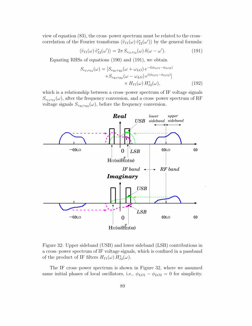
view of equation (83), the cross–power spectrum must be related to the cross–correlation of the Fourier transforms 〈vI1(ω) v∗I2(ω

′)〉 by the general formula:

〈vI1(ω) v∗I2(ω′)〉 = 2π SvI1vI2

(ω) δ(ω − ω′). (191)

Equating RHSs of equations (190) and (191), we obtain

SvI1vI2(ω) = [SvR1vR2

(ω + ωLO) e−i(φLO1−φLO2)

+SvR1vR2(ω − ωLO) ei(φLO1−φLO2)]

×HI1(ω)H∗I2(ω), (192)

which is a relationship between a cross–power spectrum of IF voltage signalsSvI1vI2

(ω), after the frequency conversion, and a cross–power spectrum of RFvoltage signals SvR1vR2

(ω), before the frequency conversion.

ω

Real

Imaginary

ωLO−ωLO 0

ωLO−ωLO 0 ω

IF band RF band

USB

LSB

USB

LSB

HI1(ω)HI2(ω)*

HI1(ω)HI2(ω)*

upper sideband

lower sideband

Figure 32: Upper sideband (USB) and lower sideband (LSB) contributions ina cross–power spectrum of IF voltage signals, which is confined in a passbandof the product of IF filters HI1(ω)H∗

I2(ω).

The IF cross–power spectrum is shown in Figure 32, where we assumedsame initial phases of local oscillators, i.e., φLO1 − φLO2 = 0 for simplicity.

89

The IF spectrum is Hermitian symmetric, according to the general propertyof a cross–power spectrum, which corresponds to a real cross–correlation,as shown in equation (60). In our case, the cross–correlation of IF voltagesignals is surely real, simply because IF voltage signals themselves are real.

Since the cross–correlation can be described by the positive–frequency re-gion of the Hermitian symmetric cross–power spectrum, as we saw in equation(62), we will pay our attension to the positive frequency region (ω ≥ 0) of theIF spectrum. Then, the original RF cross–power spectrum, shown by solidlines in Figure 32, is down–converted to IF–band, and the upper sideband(USB) of SvR1vR2

(ω+ωLO) (shown by a broken line), and the lower sideband(LSB) of SvR1vR2

(ω − ωLO) (shown by a dotted line) are passed through theproduct of the IF filters HI1(ω)H∗

I2(ω) in the positive IF frequency region,as we see in Figure 32.

Thus, we can notice here following properties of the IF spectrum:

• Spectral shape of the RF spectrum is preserved, and just shifted intothe IF–band.

• Upper sideband (USB) and lower sideband (LSB) components are su-perposed in the IF passband of HI1(ω)H∗

I2(ω).

• In the positive frequency range of the IF spectrum, ω ≥ 0, spectrum ofthe LSB component is reversed, compared with the positive frequencypart of the original RF spectrum.

Because of the Hermitian symmetry Sxy(−ω) = S∗xy(ω) for real processes,

as shown in equation (60), we can rewrite equation (192) in a form:

SvI1vI2(ω) = [SvR1vR2

(ωLO + ω) e−i(φLO1−φLO2)

+S∗vR1vR2

(ωLO − ω) ei(φLO1−φLO2)]

×HI1(ω)H∗I2(ω), (193)

using only positive–frequency part of the RF cross–power spectrum. Thefirst term in the RHS of equation (193) shows USB component in the pos-itive frequency side (ω ≥ 0) and LSB component in the negative frequencyside (ω < 0), while the second term shows LSB component in the positivefrequency side (ω ≥ 0) and USB component in the negative frequency side(ω < 0).

90

2.3 Delay Tracking and Fringe Stopping

In subsection 1.3, we saw, based on a simple interferometer model, that aradio interferometer can detect a radio source, only when the source is withinthe “coherence interval” of the white fringe, i.e., within a certain range,around zero, of the delay between arrival times of a common wave front,from an astronomical radio source, at antennas. The delay range is roughlyequal to 2/B, where B is a frequency bandwidth of the received signal. Table1 of subsection 1.3.6 showed that the delay range corresponds to an angularinterval in the sky, which is usually very narrow for modern interferometers,especially for VLBIs. If we do not have any effective means to compensate thedelay, this would imply that we can observe a source, only when the sourcehappens to be within the very narrow region of the sky, where the geometricdelay is nearly zero, that is, of course, highly ineffective and unrealistic.

Also, we saw that the diurnal motion of a radio source causes rapid oscil-lation of the correlator output due to the densely spaced fringe patterns, asschematically illustrated in Figure 21 and Table 2 of subsection 1.3.7. Suchan oscillation would make it practically impossible to integrate the multi-plier output for a duration of time, sufficient to get a signal to noise ratio,necessary for detecting the source.

Therefore, the modern interferometers must be equipped with specialmechanisms, for compensating the delay and stopping the rapid oscillationof the correlator output. They are called “delay tracking” and “fringe stop-ping”, respectively. Now we would like to discuss how these functions arerealized in a relaistic interferometer.

2.3.1 General Form of Cross–Power Spectrum of IF Signals

In order to clarify meanings of the delay tracking and fringe stopping inmore detail, we will first combine results of previous discussions, and derivea general description of the cross–power spectrum of IF voltage signals.

So far, we derived

1. the cross–power spectrum of received voltages:

Sv1v2(ω) =1

4A0 e

−iωτg0 V(ω),

given in equation (168), where A0 is the geometrical mean of effectiveapertures of antennas, and V(ω) is the complex visibility:

V(ω) =∮

AN (σ) Iν(σ) e−i2πDλ·σ dΩ,

91

given in equation (165), where AN(σ) is the normalized power patternof an interferometer, σ = s − s0 is an offset vector showing a certaindirection s in a source with respect to the reference direction s0, Iν(σ)is the source intensity distribution, and Dλ = D/λ is a baseline vectornormalized by a wave length λ,

2. the cross–power spectrum of RF voltage signals after the RF filters(amplifiers and BPFs) with system functions HR1(ω) and HR2(ω):

SvR1vR2(ω) = Sv1v2(ω)HR1(ω)H∗

R2(ω),

given in equation (177),

3. the cross–power spectrum of IF voltage signals after the frequency con-version:

SvI1vI2(ω) = [SvR1vR2

(ωLO + ω) e−i(φLO1−φLO2)

+S∗vR1vR2

(ωLO − ω) ei(φLO1−φLO2)]

×HI1(ω)H∗I2(ω),

given in equation (193), where ωLO is the LO reference frequency, φLO1

and φLO2 are initial phases of two local oscillators, and HI1(ω) andHI2(ω) are system functions of the IF filters.

Combining last two equations, i.e., equations (177) and (193), we have

SvI1vI2(ω)

= [HR1(ωLO + ω)H∗R2(ωLO + ω)Sv1v2(ωLO + ω) e−i(φLO1−φLO2)

+H∗R1(ωLO − ω)HR2(ωLO − ω)S∗

v1v2(ωLO − ω) ei(φLO1−φLO2)]

×HI1(ω)H∗I2(ω). (194)

Here, system functions of real impulse responses of IF filters must satisfyequation (74):

HI1(ω) = H∗I1(−ω), and H∗

I2(ω) = HI2(−ω).

Therefore, introducing new system functions H1(ω) and H2(ω) for responsesof combined IF filters, composed of down–converted RF and original IF fil-ters, in antenna 1 and antenna 2, respectively:

H1(ω) = HR1(ωLO + ω)HI1(ω),

H2(ω) = HR2(ωLO + ω)HI2(ω), (195)

92

we can rewrite equation (194) as:

SvI1vI2(ω)

= H1(ω)H∗2(ω)Sv1v2(ωLO + ω) e−i(φLO1−φLO2)

+H∗1 (−ω)H2(−ω)S∗

v1v2(ωLO − ω) ei(φLO1−φLO2). (196)

Hereafter, we call the complex function H1(ω)H∗2(ω) “bandpass characteris-

tics of combined IF filters”.Then, inserting equation (168) into equation (196), we obtain a general

form of the cross–power spectrum of the IF voltage signals, which describesSvI1vI2

(ω) in terms of source intensity distribution, geometry of observation,filter responses, and parameters of the frequency conversion:

SvI1vI2(ω)

=1

4A0 e−i[(ωLO+ω)τg0+φLO1−φLO2] V(ωLO + ω)H1(ω)H∗

2(ω)

+ei[(ωLO−ω)τg0+φLO1−φLO2] V∗(ωLO − ω)H∗1(−ω)H2(−ω).

(197)

Of course, this equation satisfies the Hermitian symmetry condition:

SvI1vI2(ω) = S∗

vI1vI2(−ω),

required for real processes vI1(t) and vI2(t).Representing the complex visibility in terms of visibility amplitude and

visibility phase, as introduced in equation (166), we have

V(ωLO + ω) = | V(ωLO + ω) | eiΦv(ωLO+ω),

V∗(ωLO − ω) = | V(ωLO − ω) | e−iΦv(ωLO−ω). (198)

Also we represent the bandpass characteristics of combined IF filters in termsof its amplitude | H1(ω)H∗

2(ω) | and phase Φb(ω):

H1(ω)H∗2(ω) = | H1(ω)H∗

2(ω) | eiΦb(ω),

H∗1 (−ω)H2(−ω) = | H1(−ω)H∗

2(−ω) | e−iΦb(−ω). (199)

Then, the cross–power spectrum of IF signals is now reduced to

SvI1vI2(ω)

=1

4A0 | V(ωLO + ω) | | H1(ω)H∗

2(ω) | e−i[(ωLO+ω)τg0+φLO1−φLO2−Φv(ωLO+ω)−Φb(ω)]

+1

4A0 | V(ωLO − ω) | | H1(−ω)H∗

2(−ω) | ei[(ωLO−ω)τg0+φLO1−φLO2−Φv(ωLO−ω)−Φb(−ω)].

(200)

93

Again, first term in the RHS of equation (200) shows USB component inthe positive frequency range (ω ≥ 0) and LSB component in the negativefrequency range (ω < 0), while second term shows LSB component in thepositive frequency range (ω ≥ 0) and USB component in the negative fre-quency range (ω < 0).

amplitude

phaseω

ω

ωLO

ωLO−ωLO

−ωLO 0

0

USB LSB LSB USB

Figure 33: Amplitudes and phases of two terms in a cross–power spectrumof IF voltage signals. Solid lines show original RF spectrum, and dotted andbroken lines correspond to first and second terms of the RHS of equation(200), respectively. For simplicity, only contribution of geometric delay isshown in phase spectrum.

If we denote amplitudes and phases of the first and second terms of theRHS of equation (200) as Ap(ω), Φp(ω, t) and An(ω), Φn(ω, t), respectively,we have

SvI1vI2(ω) = Ap(ω) e−iΦp(ω, t) + An(ω) e−iΦn(ω, t), (201)

with

Ap(ω) =1

4A0 | V(ωLO + ω) | | H1(ω)H∗

2(ω) |,

An(ω) =1

4A0 | V(ωLO − ω) | | H1(−ω)H∗

2(−ω) |, (202)

94

and

Φp(ω, t) = (ωLO + ω)τg0 + φLO1 − φLO2 − Φv(ωLO + ω) − Φb(ω),

Φn(ω, t) = −(ωLO − ω)τg0 − φLO1 + φLO2 + Φv(ωLO − ω) + Φb(−ω).

(203)

Here, we took into account that phases are functions of both frequency andtime, in view of the time–variable geometric delay τg0 . This shows amplitudeand phase spectra of the cross–power spectrum of IF signals, which can becontrasted to those given in equations (101), (102), and (103), for a simpleinterferometer model. Again, first term in the RHS of equation (200) showsUSB component in the positive frequency range (ω ≥ 0) and LSB componentin the negative frequency range (ω < 0), while second term shows LSBcomponent in the positive frequency range (ω ≥ 0) and USB component inthe negative frequency range (ω < 0).

Figure 33 shows the amplitude and phase spectra of two terms of theIF cross–power spectrum in the RHS of equation (200), which can be com-pared with Figure 19 for a simple interferometer. For simplicity, we showedonly contribution of geometric delay τg0 in this figure, ignoring small effectsof φLO1, φLO2, Φv, and Φb terms. The IF band here is assumed to be a“video–band” (or “baseband”), which includes zero frequency, or “DC (di-rect current)”, component with ω = 0.

2.3.2 “Expected Correlation” of IF Signals

If we had an idealized correlator, which would be capable of multiplyingtwo IF voltage signals, and immediately calculating a statistical mean of theproduct, such a correlator would yield the cross–correlation of the IF voltagesignals RvI1vI2

(τ) at time difference τ = 0:

〈vI1(t) vI2(t)〉 = RvI1vI2(0).

According to equation (197), we expect that this “instantaneous correla-tor output” is described by an inverse Fourier transformation of the cross–power spectrum SvI1vI2

(ω), with τ = 0:

RvI1vI2(0) =

1

2π

∞∫

−∞

SvI1vI2(ω) dω =

1

π<

∞∫

0

SvI1vI2(ω) dω

=A0

4π<

e−i(ωLOτg0+φLO1−φLO2)

∞∫

0

V(ωLO + ω) e−iωτg0 H1(ω)H∗2(ω) dω

+ ei(ωLOτg0+φLO1−φLO2)

∞∫

0

V∗(ωLO − ω) e−iωτg0 H∗1 (−ω)H2(−ω) dω

, (204)

95

where we used the property of a Hermitian symmetric cross–power spectrumgiven in equation (74), in order to restrict range of integration to the positivefrequency side only.

ω I−ω I 0

∆ω∆ω

ω

G

H1(ω)H2(ω)*

Figure 34: Rectangular response of a real filter.

If we assume, similarly to what we did in the case of a simple interfer-ometer model in Section 1.3, a real, even, and rectangular system functionsof the combined IF filters, with a gain factor G, bandwidth ∆ω = 2πB andcenter frequency ωI , as shown in Figure 34, i.e.,

H1(ω)H∗2(ω) = H∗

1 (−ω)H2(−ω) =

G if ωI − ∆ω2

≤| ω |≤ ωI + ∆ω2,

0 otherwise,

(205)

and also assume a continuum spectrum source, with almost constant complexvisibility across the frequency bandwidth,

V(ω) ∼= V for ωI −∆ω

2≤| ω |≤ ωI +

∆ω

2, (206)

then, we obtain from equation (204)

RvI1vI2(0) =

A0G

4π<

e−i(ωLOτg0+φLO1−φLO2) VωI+∆ω

2∫

ωI−∆ω2

e−iωτg0 dω

+ ei(ωLOτg0+φLO1−φLO2) V∗

ωI+∆ω2

∫

ωI−∆ω2

e−iωτg0 dω

. (207)

Since the integral in equation (207) is described in terms of the sinc function,as we saw in equation (100):

1

π

ωI+∆ω2

∫

ωI−∆ω2

e−iωτg0 dω = 2Be−iωIτg0sin(πBτg0)

πBτg0,

96

and the complex visibility is represented in terms of its amplitude and phase:

V =| V | eiΦv ,

equation (207) is further reduced to

RvI1vI2(0) =

A0GB | V |2

sin(πBτg0)

πBτg0× [cos(ωLOτg0 + ωIτg0 + φLO1 − φLO2 − Φv)

+ cos(ωLOτg0 − ωIτg0 + φLO1 − φLO2 − Φv)].

(208)

This equation is an analog of eauation (100), which we derived for a simpleinterferometer model observing a continuum spectrum source. The sinc func-tion stands for a bandwidth pattern, and two cosine terms are fringe patternscorresponding to center frequencies of USB and LSB, respectively. Evidently,first cosine term shows contribution of USB component, while second cosineterm shows contribution of LSB component.

Equation (208) again shows that we can detect fringe pattern of a contin-uum spectrum source within a narrow coherence interval, roughly representedby ∆τB = 2/B. Also, time variation of the geometric delay τg0 in the fringepatterns causes rapid sinusoidal oscillation of RvI1vI2

(0), which makes it al-most impossible to integrate (time–average) the product of voltage signalsfor a meaningful duration of time. Therefore, we definitely need the delaytracking and fringe stopping for a realistic interferometer.

There is no widely–accepted name for the “instantaneous correlator out-put” RvX1vX2

(0), where vX1(t) and vX2(t) could be any voltages in radiointerferometry, i.e., they could be received voltages, RF voltages, or IF volt-ages. This is not an actual correlator output, since any correlator outputis obtained only after integration of a product of voltages, or a multiplieroutput, for some duration of time in an integrator. This is not the productof individual voltages, either. This is a statistical expectation of the productof voltages, or the multiplier output, at a certain instance of time.

An important point here is the following. We consider that an actualproduct of voltages consists of a signal component and a noise component,and the signal component is described by this quantity: RvX1vX2

(0). Weapply the fringe stopping, in order to stop the rapid oscillation of this signalquantity, so that we can suppress the noise and detect the signal by timeaveraging.

Hereafter, we call this quantity as an “expected correlation” in a radiointerferometer.

97

2.3.3 Radio Source Tracking by an Interferometer

What is needed is to compensate the geometric delay τg0 to get the sameeffect, which would be obtained, if we move one of the antennas along thesurface of a sphere of diameter equal to the baseline length, such that τg0 isalways maintained equal to zero, as illustrated in Figure 35. Such compensa-

multiplier

integrator

Dcτg = D sinθ

θ

correlator

h2

instrumentaldelay

τi

h1

1 2

vR2(t)vR1(t)

vR2(t)’

0

Figure 35: How to track a radio source by an interferometer? Insertion of aninstrumental delay, which compensates the geometric delay, in the RF–bandcan do the job.

tion of the geometric delay enables an interferometer to “track” the motionof a radio source, in order to keep the source in its “interferometer beam”,just as a single–dish radio telescope does with its antenna beam.

A time–variable delay circuit, which is inserted into the transmission sys-tem of one of the antennas at RF–band, and provides an instrumental delay

98

τi equal to the geometric delay τg0 , as illustrated in Figure 35, can realize, atleast theoretically, the required tracking.

Although this statement must be intuitively obvious, it would be stilluseful to logically trace the effect of delay insertion, in the following way.

Insertion of an instrumental delay τi, in the RF signal transmission systemof antenna 2, would make the RF voltage signal v ′R2(t), after the delay circuit,and its Fourier transform v′R2(ω), to be equal to

v′R2(t) = vR2(t− τi), and therefore, v′R2(ω) = vR2(ω) e−iωτi, (209)

where vR2(t), and vR2(ω), correspond to the RF voltage signal before theinstrumental delay. We used the shift theorem given in equation (68), inderiving equation (209).

Therefore, taking a cross–correlation of Fourier transforms vR1(ω) andv′R2(ω) of RF voltage signals, we see

〈vR1(ω) v′∗R2(ω′)〉 = 〈vR1(ω) v∗R2(ω

′)〉 eiω′τi . (210)

Since we assumed that the RF signals vR1(t) and vR2(t) are jointly station-ary random processes, vR1(t) and v′R2(t) must also be jointly stationary ran-dom processes. Hence, the cross–correlations of their Fourier transforms andcross–power spectra must be related to each other as:

〈vR1(ω) v′∗R2(ω′)〉 = 2πSvR1v

′

R2(ω) δ(ω − ω′),

〈vR1(ω) v∗R2(ω′)〉 = 2πSvR1vR2

(ω) δ(ω − ω′), (211)

in view of equation (83). Comparing equations (210) and (211), we obtaina relation between the cross–power spectrum SvR1v

′

R2(ω) of the RF voltage

signal vR1(t) of antenna 1 and the delay–inserted RF voltage signal v ′R2(t)of antenna 2, and the cross–power spectrum SvR1vR2

(ω) of the RF voltageswithout delay insertion:

SvR1v′

R2(ω) = SvR1vR2

(ω) eiωτi, (212)

which leads to

SvR1v′

R2(ω) = Sv1v2(ω)HR1(ω)H∗

R2(ω) eiωτi

=1

4A0 e

−iω∆τg V(ω)HR1(ω)H∗R2(ω), (213)

where∆τg = τg0 − τi.

99

We used here equations (168) and (177) for expressions of the cross–powerspectra of RF voltages SvR1vR2

(ω), and received voltages Sv1v2(ω).As we see, an only different point between combined equations (168) and

(177) and this equation (213) is that the geometric delay τg0 is replaced bythe delay difference ∆τg = τg0 − τi. Therefore, we can easily derive an ex-pected correlation of an IF voltage vI1(t) of antenna 1 and an IF voltage withdelay inserted at RF–band v′′I2 of antenna 2, RvI1v′′I2

(0), from equation (208),assuming again a rectangular filter, given in equation (205), and constantvisibility over receiving bandwidth, given in equation (206). The result is

RvI1v′′

I2(0) =

A0GB | V |2

sin(πB∆τg)

πB∆τg× [cos(ωLO∆τg + ωI∆τg + φLO1 − φLO2 − Φv)

+ cos(ωLO∆τg − ωI∆τg + φLO1 − φLO2 − Φv)].

(214)

Thus, as long as τi = τg0 , no delay effect is left in the RF cross–powerspectrum, given in equation (213), and, therefore, also in the expected corre-lation of IF voltages in equation (214). This means that the insertion of aninstrumental delay, exactly equal to the geometric delay, at RF–band couldeffectively reduce τg in equation (100), or τg0 in equation (208), to zero. Thiswould allow us to find fringes always at the center of the coherence interval,and to integrate the product of voltage signals, as long as we wish. Or, oth-erwise speaking, we could realize both delay tracking and fringe stopping bya single operation, namely by the insertion of a time variable instrumentaldelay, if we were allowed to do this at RF–band.

Unfortunately, it is almost impossible, in the current level of technology,to realize any delay insertion at RF frequencies, higher than several GHz.Therefore, the delay insertion is usually performed at IF–band.

2.3.4 Requirements to the Delay Tracking and Fringe Stopping

Before proceeding with discussions on actual realization of the delay track-ing and fringe stopping, let us here estimate the ranges of variations, andacuracies required to theoretical predictions, of the geometric delay τg0 andits time rate τg0 . For simplicity, we will implicitly rely upon an image of thedelay insertion at RF–band discussed above, since this does not cause anyloss of generality in present discussions.

If we denote the baseline vector and the unit vector directed to the radiosource as D and s0, respectively, the geometric delay τg0 and its time rate

100

τg0 , due to the diurnal rotation of the Earth, are given by:

τg0 =D · s0

c, (215)

τg0 =D · s0

c=

(ω × D) · s0

c, (216)

where ω is the angular velocity vector of the rotation of the Earth (|ω| '7.3 × 10−5 rad/sec) and c ' 3 × 108 m/sec is the light velocity. Of course,equation (216) is valid for ground–based interferometers only, and not validfor space–VLBI baselines.

For a connected–element radio interferometer (CERI) of 300 m baseline,say, the maximum geometric delay:

τgmax=D

c= 1 µsec,

is obtained when the source direction is parallel to the baseline, and themaximum delay rate:

τgmax=ωD

c= 70 psec/sec,

is obtained when ω ⊥ D and (ω × D) ‖ s0.

ω

D

R

2R

Figure 36: The maximum geometric delay (top) and maximum delay rate(bottom) of the ground–based VLBI.

For the ground–based VLBI, the maximum geometric delay and the max-imum delay rate are obtained in cases shown in Figure 36. If we denote theEarth’s radius as R⊕ = 6300 km, the maximum values are

τgmax=

R⊕

c= 21 msec, (217)

τgmax=

2R⊕ω

c= 3.1 µsec/sec. (218)

101

If we observe at 22 GHz, equations (208) and (218) implies that the expectedcorrelation, defined in subsection 2.1.8, may oscillate with frequency as highas 22 GHz × 3.1 × 10−6 = 68.2 kHz, or 68,200 cycles per second(!), dueto the diurnal motion of the source across the fringe pattern. Indeed, nomeaningful integration of the multiplier output is possible, unless we stopsuch an oscillation.

The ranges of variations of geometric delay and its rate, as examinedabove, and resulting variations of the phase in the cross-power spectrum ofvoltage signals, such as shown in equation (200), are orders of magnitudelarger, than those caused by other delay effects (clock offset, atmosphericpropagation delay, cable delay, etc.), and by other phase terms (LO initialphase, visibility phase, phase of bandpass characteristics, etc.). Therefore,the delay tracking and fringe stopping are, primarily, means for compensationof geometric delay. Although some other, much smaller, effects are also takeninto account in highly precise delay tracking and fringe stopping, performedin VLBI correlators, we will postpone discussion of this problem, until weconsider correlation processings in VLBI.

We use an appropriate theoretical prediction of the time–variable geo-metric delay, in order to determine length and rate of the instrumental delay,to be applied to actual delay tracking and fringe stopping. Hence, the the-oretical prediction itself, for the geometric delay τg0, has been traditionallydenoted as τi, and called “instrumental delay”.

Let us estimate accuracies required to such an instrumental delay τi andits rate τi.

In order to get a white fringe near the peak of the bandwidth pattern,a difference ∆τg between the actual geometric delay τg0 and the predictedinstrumental delay τi, which we call hereafter “residual delay”:

∆τg = τg0 − τi, (219)

must be kept well smaller than the coherence interval ∆τB = 2/B, where Bis an observing bandwidth:

∆τg ∆τB =2

B. (220)

Therefore, the acuuracy of the instrumental delay must be much better than1 µsec when B = 2 MHz, and much better than 1 nsec when B = 2 GHz, asTable 1 shows. We now compare these required accuracies with maximumdelay values τgmax

, estimated above for 300 m baseline connected–elementradio interferometer (CERI), and for VLBI. Table 3 shows relative accuracy,in terms of ∆τg/τgmax

, required to the instrumental delay. The Table shows

102

300 m CERI VLBI

τgmax= 1µsec τgmax

= 21 msec

B = 2 MHz (∆τg 1 µsec) 1 5 × 10−5

B = 2 GHz (∆τg 1 nsec) 10−3 5 × 10−8

Table 3: Relative accuracy of ∆τg/τgmaxrequired to the instrumental delay.

that the required accuracy is rather high, for VLBI.On the other hand, in order to carry out integration of the multiplier

output in a correlator, for a duration of time sufficient to get high enoughS/N ratio, we must apply an accurate theoretical model τi(t) to compensatefor time variation of the geometric delay τg0. If integration time is τa andobserving frequency is ν, a requirement to ∆τg = (τg0 − τi) for successfulintegration, is traditionally given by

2πν∆τgτa ≤ 1. (221)

This requirement corresponds to a condition that an accumulated change ofthe phase of the cross–power spectrum of voltage signals, such as shown inequation (213), or of the phase in cosine terms of the expected correlationin equation (214), does not exceed 1 radian during the integration time τa.Table 4 shows required accuracy of the residual delay rate ∆τg, according to

300 m CERI VLBI

τa = 1000 s, τgmax= 70 ps/s τa = 1 s , τgmax

= 3.1µs/s

ν = 10 GHz ≤ 1.6 ×10−2 ps/s (≤ 2.3 ×10−4) ≤ 16 ps/s (≤ 5.2 ×10−6)

ν = 100 GHz ≤ 1.6 ×10−3 ps/s (≤ 2.3 ×10−5) ≤ 1.6 ps/s (≤ 5.2 ×10−7)

Table 4: Required accuracy of ∆τg and relative accuracy of ∆τg/τgmax(in

parenthes) for a 300 m baseline CERI with integration time τa = 1000 sand maximum delay rate τgmax

= 70 ps/s, and a VLBI with integration timeτa = 1 s and maximum delay rate τgmax

= 3.1 µs/s .

equation (221), and its ratio to the maximum delay rate, estimated above,for a 300 m baseline CERI with a typical integration time τa = 1000 s, and aVLBI with a typical hardware integration time with a VLBI correlator τa = 1s, at two cases of observing frequency, ν = 10 GHz and ν = 100 GHz.

103

The requred accuracies are fairly high, especially in VLBI. Therefore,theoretical prediction of the instrumental delay is usually based on state–of–the–art geophysical and astronomical models of station coordinates, radiosource coordinates, and irregularities in the rotational motion of the Earth.

2.3.5 Insertion of Instrumental Delay at IF Band

Let us consider a case, when a time–variable instrumental delay τi is insertedin the IF–band signal transmission system of antenna 2, as illustrated inFigure 37.

Dcτg = D sinθ

θ

multiplier

integrator

τi

correlator

LO

instrumentaldelay

Figure 37: Time–variable instrumental delay inserted at IF–band.

After the insertion of the delay circuit, IF voltage signal v ′I2(t), and itsFourier transform v′I2(ω), are changed to

v′I2(t) = vI2(t− τi), and, therefore, v′I2(ω) = vI2(ω) e−iωτi, (222)

104

where vI2(t), and vI2(ω), correspond to the IF voltage signal before the in-strumental delay. We again used the shift theorem given in equation (68),for deriving equation (222).

Following discussions in Subsection 2.3.3, we take a cross–correlation ofFourier transforms vI1(ω) and v′I2(ω) of IF voltage signals, to obtain

〈vI1(ω) v′∗I2(ω′)〉 = 〈vI1(ω) v∗I2(ω

′)〉 eiω′τi . (223)

Since the IF signals vI1(t) and v′I2(t), as well as vI1(t) and vI2(t), are assumedto be jointly stationary random processes, the cross–correlations of theirFourier transforms and cross–power spectra are related to each other, byequation (83), as:

〈vI1(ω) v′∗I2(ω′)〉 = 2πSvI1v

′

I2(ω) δ(ω − ω′),

〈vI1(ω) v∗I2(ω′)〉 = 2πSvI1vI2

(ω) δ(ω − ω′). (224)

Comparing equations (223) and (224), we see that the cross–power spec-trum SvI1v′I2

(ω) of the IF voltage signal vI1(t) of antenna 1 and the delay–inserted IF voltage signal v′I2(t) of antenna 2, and the cross–power spectrumSvI1vI2

(ω) of the IF voltages without delay insertion, are related to each otheras:

SvI1v′

I2(ω) = SvI1vI2

(ω) eiωτi. (225)

Inserting equation (197) to this equation, we have

SvI1v′

I2(ω)

=1

4A0 e−i[ωLO τg0+ω∆τg+φLO1−φLO2] V(ωLO + ω)H1(ω)H∗

2(ω)

+ei[ωLO τg0−ω∆τg+φLO1−φLO2] V∗(ωLO − ω)H∗1(−ω)H2(−ω),

(226)

where, again, ∆τg = τg0 − τi is the residual delay. Contrary to equation(213), which describes the effect of the delay insertion at RF–band, we cannothere completely compensate for the geometric delay τg0, even if we insert aninstrumental delay which is exactly equal to the geometric delay τi = τg0 . Infact, a term ωLOτg0 is still left uncompensated in the exponential functionsof equation (226).

In order to see this point more clearly, let us derive the expected corre-lation RvI1v

′

I2(0), as we did in equation (207), assuming again a rectangular

filter, given in equation (205), and constant visibility over receiving band-width, given in equation (206). Since everything is the same as given in

105

equation (207), except for a coefficient of ω term in the exponential func-tions, namely ω∆τg instead of ωτg0, we obtain the result of integration:

RvI1v′

I2(0) =

A0GB | V |2

sin(πB∆τg)

πB∆τg× [cos(ωLOτg0 + ωI∆τg + φLO1 − φLO2 − Φv)

+ cos(ωLOτg0 − ωI∆τg + φLO1 − φLO2 − Φv)],

(227)

where ωI is the IF band center frequency, which is similar to equation (208),except in the argument of sinc function and in the coefficient of ωI term incosine functions.

It is evident, from this equation, that insertion of an instrumental delayτi, which is equal to the geometric delay τg0 , at IF–band, enables us todetect a white fringe at the center of the coherence interval. However, ωLOτg0terms in arguments of cosine functions are left uncompensated, which willcause enormously rapid oscillations of the expected correlation. Therefore,insertion of an instrumental delay at IF–band can perform the delay tracking,but not the fringe stopping.

2.3.6 Separation of Delay Tracking and Fringe Stopping Due toFrequency Conversion

The reason, why the insertion of the instrumental delay at IF–band canperform only the delay tracking, but not the fringe stopping, may be easilyunderstood by examining Figure 38, which illustrates a time variation of thephase spectrum of IF voltage signals shown in Figure 33, in a particular caseof a single–sideband reception of USB component.

Let us consider phase spectra in cross–power spectra of voltage signalswithout delay insertion, and compare the phase spectrum in IF–band withthe one in RF band. In doing so, we ignore minor phase terms, such as LOinitial phase, visibility phase, and phase of bandpass characteristics, whichfigure in equation (200), leaving only the main term due to the geometricdelay.

Then, the phase spectrum in RF–band is a straight line crossing theorigin, with inclination equal to the geometric delay τg0 , as shown in equation(103) and Figure 19 for a simple interferometer model, or in equations (168),and (177), for a more realistic interferometer.

However, after the frequency conversion, the phase spectrum in the IF–band no longer crosses the origin, since the frequency conversion shifts the

106

phasephase phase

phasephase phase

phasephase phase

= +

= +

= +

phase phasephase

= +

IF RF object ofdelaytracking

object offringestopping

τg

ω

ω ω

ω

ω

ω

ω

ω

0

Figure 38: Necessity of fringe stopping, besides delay tracking in IF–band.We assume here a USB single–sideband reception, and show only positivefrequency range of the phase spectrum, except in the bottom panel.

107

band–limited spectrum at RF–band to IF band without changing its shape,as shown in Figures 32, 33, and 38.

Therefore, the frequency converted phase spectrum in IF–band is nowrepresented by a sum of two components, namely an inclined straight lineωτg0, crossing the origin, plus a frequency–independent phase shift equal toωLOτg0, where ωLO is the LO frequency, as illustrated in the right panels ofFigure 38 and in equation (200). This phase shift rapidly changes in time,with the speed as high as several tens kHz (as we saw in the example of anintercontinental VLBI observation with 22 GHz), due to the diurnal variationof the geometric delay τg0.

The insertion of the instrumental delay at the IF–band compensates forthe first component, i.e. reduces the phase slope across the frequency bandto nearly zero, and thus makes it possible to get a white fringe in the mid-dle of the coherence interval, as evident from equation (208). However, theinstrumental delay in the IF–band does not compensate for the second com-ponent at all. Therefore, we still need to compensate for the rapid phase shiftin the second component, by somehow controlling the interferometer phase.This operation is the “fringe stopping”, which is separated from the “delaytracking” after the frequency conversion.

2.3.7 Actual Implementations of Delay Tracking

In early history of radio interferometry, analog delay cables, as schematically

transmission cable

delay cables

Figure 39: Analog delay cables used for delay tracking in early history ofradio interferometry.

illustrated in Figure 39, were used for delay tracking. N delay cables withlengths τ0, 2τ0, 4τ0, 8τ0, · · ·, 2N−1τ0, were mechanically inserted into, andremoved from, a signal transmission cable of an interferometer, to realizea time variable instrumental delay τi with a range of variation: τ0 ≤ τi ≤(2N − 1)τ0. Of cource, the longest delay cable must have a length as largeas about a half of baseline length of the interferometer. Therefore, such

108

analog delay cables could be used for connected–element interferometers withbaseline lengths of several hundreds meters, but definitely not for VLBIs.

writeaddress

readaddress

delay

input data

delayed output data

ring buffer

Figure 40: A “ring buffer” used for digital delay tracking.

Recently, most of radio interferometers, including VLBIs, use digital delaycircuits for delay tracking. In order to use this technique, data signal is firstdigitized, and then fed to a bulk memory, which is a kind of “ring buffer”,schematically shown in Figure 40.

Data are written to, and read from, the ring buffer at different addresses,and these write and read addresses are incremented by one at each “clocktiming pulse” of digital circuit. An interval of succcessive clock timing pulsescorresponds to a sampling interval ts of digitization of the data. Thus, ifthe difference between the write and read addresses in the ring buffer isn, an instrumental delay equal to nts is realized in this way. And furthershifting the write (or read) address periodically, once per a certain numberof clock timing pulses, we can vary this instrumental delay in time. We willexamine this digital delay tracking in more detail, when we will discuss VLBIcorrelators.

2.3.8 Actual Implementations of Fringe Stopping

In connected–element interferometers, the fringe stopping is often carried outby actively controlling the initial phases φLO1 and φLO2 of the LO referencesignals, as illustrated in Figure 41, so that

φLO1(t) − φLO2(t) = −ωLO τi(t) + ψLO1 − ψLO2, (228)

109

Dcτg = D sinθ

θ

multiplier

integrator

delaytracking

τi

correlator

LOΦLO1(t) fringe

stoppingΦLO2(t)

Figure 41: Fringe stopping by active control of LO initial phases.

where ψLO1 − ψLO2 is a nearly constant part of the difference of the initialphases of the LO signals, and τi is the instrumental delay, i.e., the theoreticalprediction of the geometric delay τg0 .

Assuming quasi–static LO initial phases, similarly to what we did insubsection 2.1.8 for the geometric delay, we can just insert equation (228) toequation (226) for the cross–power spectrum of IF voltages, and to equation(227) for the expected correlation in the case of a continuum flat spectrumsource and rectangular filters, after the delay tracking at IF–band. Then, weobtain the cross–power spectrum of IF voltages:

SfvI1v′

I2(ω)

=1

4A0 e−i[ωLO ∆τg+ω∆τg+ψLO1−ψLO2] V(ωLO + ω)H1(ω)H∗

2(ω)

+ei[ωLO ∆τg−ω∆τg+ψLO1−ψLO2] V∗(ωLO − ω)H∗1(−ω)H2(−ω),

(229)

and expected correlation:

RfvI1v

′

I2(0) =

A0GB | V |2

sin(πB∆τg)

πB∆τg

110

× [cos(ωLO∆τg + ωI∆τg + ψLO1 − ψLO2 − Φv)

+ cos(ωLO∆τg − ωI∆τg + ψLO1 − ψLO2 − Φv)],

(230)

respectively.Now we can stop the rapid phase changes in the cross–power spectrum,

as well as in the expected correlation, provided that we can always keep theresidual delay to be nearly zero:

∆τg = τg0 − τi ∼= 0.

Note that this active control of LO initial phases can stop the phasechanges both in USB and LSB components of the cross–power spectrum andexpected correlation of IF voltages, as evidenced by equations (229) and(230). In particular, arguments of first and second cosine terms in the RHSof equation (230), which show USB and LSB contributions, respectively, areboth stopped by this operation.

Another method for fringe stopping, which has been applied to VLBIdigital correlators, in particular, uses multiplication of a sinusoidal functionof time to an IF voltage, as shown in Figure 42.

Dcτg = D sinθ

θ

multiplier

integrator

delaytracking

τi

correlator

LO

2 cos(ωLO τi)

fringe stopping

antenna 1 antenna 2

vI2(t)

vI1(t)

’vI1(t)f

Figure 42: Fringe stopping by multiplication of a sinusoidal function.

111

In this method, a sinusoidal function

2 cos(ωLOτi), (231)

where ωLO is the LO frequency, and τi is the theoretically predicted instru-mental delay, is multiplied to IF voltage vI1(t) of antenna 1.

Assuming again that ωLOτi is a quasi–static quantity, we obtain for a newIF voltage vfI1(t) of antenna 1 after the multiplication of 2 cos(ωLOτi):

vfI1(t) = vI1(t)2 cos(ωLOτi) = vI1(t)(eiωLOτi + e−iωLOτi), (232)

and for its Fourier transform vfI1(ω):

vfI1(ω) = vI1(ω)(eiωLOτi + e−iωLOτi), (233)

where vfI1(ω) is a Fourier transform of vI1(t). Then we have a cross–correlationof Fourier transforms of IF voltages:

〈vfI1(ω)v′∗I2(ω′)〉 = 〈vI1(ω)v′∗I2(ω

′)〉(eiωLOτi + e−iωLOτi), (234)

where v′I2(ω) is the IF voltage of antenna 2 after the delay insertion. As-suming jointly stationary random processes, we obtain for a cross–powerspectrum of IF voltages vfI1(t) and v′I2(t):

SvfI1v

′

I2(ω) = SvI1v

′

I2(ω)(eiωLOτi + e−iωLOτi), (235)

where SvI1v′

I2(ω) is the cross–power spectrum of IF voltages vI1(t) and v′I2(t),

which is given in equation (226). Then, inserting equation (226) to equation(235), we have

SvfI1v

′

I2(ω) =

1

4A0

×e−i[ωLO ∆τg+ω∆τg+φLO1−φLO2] V(ωLO + ω)H1(ω)H∗2(ω)

+e−i[ωLO(τg0+τi)+ω∆τg+φLO1−φLO2] V(ωLO + ω)H1(ω)H∗2(ω)

+ei[ωLO ∆τg−ω∆τg+φLO1−φLO2] V∗(ωLO − ω)H∗1(−ω)H2(−ω)

+ei[ωLO(τg0+τi)−ω∆τg+φLO1−φLO2] V∗(ωLO − ω)H∗1(−ω)H2(−ω),

(236)

where ∆τg = τg0 − τi. In first and third terms in the RHS of this equation,rapid oscillations of exponential terms are almost stopped, as long as τi ∼= τg0 .But, in second and fourth terms in the RHS, even more rapid oscillationswith almost doubled frequency ωLO( ˙τg0 + τi) remain. Contributions of theserapidly oscillating terms almost disappear when the product of IF voltages

112

are integrated for some duration of time in a correlator. Therefore, we havean “effective” cross–power spectrum of IF voltages,

SvfI1v′

I2(ω) =

1

4A0

×e−i[ωLO ∆τg+ω∆τg+φLO1−φLO2] V(ωLO + ω)H1(ω)H∗2(ω)

+ei[ωLO ∆τg−ω∆τg+φLO1−φLO2] V∗(ωLO − ω)H∗1(−ω)H2(−ω),

(237)

which has essentially the same form as the one given in equation (229).Note that, in this simple method of multiplication of a sinusoidal func-

tion to an IF voltage, phase drifts are stopped again in both USB and LSBcomponents.

2.4 Correlator Outputs

2.4.1 Multiplier and Integrator

As we saw earlier, a key component of a correlator in an interferometer is adevice with two inputs and one output, which is composed of a multiplierand an integrator (Figure 43). The expected correlation, which is the sta-

multiplier

integrator

from antenna 1 from antenna 2

.

Figure 43: Multiplier and integrator as a key component of a correlator.

tistical expectation of the product of the voltage signals, must be containedas a signal component in a multiplier output of such a correlator. Sincethe expected correlation does not rapidly oscillate any more after the delaytracking and fringe stopping, we can integrate (time–average) the multiplier

113

output during some time to suppress the noise component, and detect thisnearly constant expected correlation itself with a high signal to noise ratio.Therefore, an output of an actual correlator can be well approximated bythe expected correlation after the delay tracking and fringe stopping. Theexpected correlation is easily derived from the cross–power spectrum (CPS)of the IF voltages by an inverse Fourier transformation, as we showed inequation (204).

Now we have slightly different notations for the CPS of IF voltages inequation (229) and in equation (237), depending on practical implementa-tions of the fringe stopping, though they are essentially equivalent to eachother. We adopt, hereafter, the expression given in equation (237), whichis familiar in VLBI practice, for describing the CPS after the delay trackingand fringe stopping.

Then, the expected correlation, after the delay tracking and fringe stop-ping, is given by

RvfI1v

′

I2(0) =

A0

4π<

e−i(ωLO∆τg+φLO1−φLO2)

∞∫

0

V(ωLO + ω) e−iω∆τg H1(ω)H∗2(ω) dω

+ ei(ωLO∆τg+φLO1−φLO2)

∞∫

0

V∗(ωLO − ω) e−iω∆τg H∗1 (−ω)H2(−ω) dω

.

(238)

In the special case of a continuum flat spectrum source and rectangular filters,the expected correlation will have essentially the same form as the one givenin equation (230):

RvfI1v′

I2(0) =

A0GB | V |2

sin(πB∆τg)

πB∆τg× [cos(ωLO∆τg + ωI∆τg + φLO1 − φLO2 − Φv)

+ cos(ωLO∆τg − ωI∆τg + φLO1 − φLO2 − Φv)].

(239)

We will use expected correlations given in equations (238) and (239) astheoretical expressions of the correlator outputs.

In VLBI, no operation for delay tracking and fringe stopping is done,usually, in observing stations. Instead, they are done in VLBI correlators.Therefore, a VLBI correlator is a little more complicated than the meremultiplier and integrator, as we will see later.

114

2.4.2 Single Sideband (USB or LSB) Reception

So far, we considered a case of double sideband (DSB) reception, i.e. a casewhen we receive signals contained in both upper sideband (USB) and lowersideband (LSB) of LO frequency in original RF–band spectrum. In this case,the USB and LSB contributions are superposed in IF–band spectrum, as wesaw earlier.

The DSB reception is not convenient for observing line spectrum sources,since different lines in USB and LSB are mixed up in the same IF spectrum.Also, the DSB reception causes additional complications in data calibrations.Therefore, in VLBI, we mostly use a single sideband (SSB), i.e., either of USBor LSB, reception.

Amplitude and phase spectra of IF voltage signals, which were shown inFigure 33 in the DSB reception case, now take simpler forms, in the SSBreception case, as shown in Figure 44.

amplitude

phaseω

ω

ωLO

ωLO−ωLO

−ωLO 0

0

USB USBamplitude

phaseω

ω

ωLO

ωLO−ωLO

−ωLO 0

0

LSB LSB

Figure 44: Amplitude and phase spectra of IF voltage signals in USB (left)and LSB (right) receptions. For simplicity, contributions of the geometricdelay only are shown in the phase spectra.

Since, cross–power spectra (CPS) of IF voltages both in USB and LSBreceptions are Hermitian symmetric, as illustrated in Figure 44, we do notlose generality if we confine ourselves to consider only positive frequencyrange (ω ≥ 0) of the spectra.

In positive frequency range ω ≥ 0, cross–power spectra of IF voltagesbefore the delay tracking and fringe stopping in USB and LSB receptions aregiven by

115

SUSBvI1vI2(ω) =

1

4A0 e

−i[ωLO τg0+ωτg0+φLO1−φLO2] V(ωLO + ω)H1(ω)H∗2(ω),

(240)

SLSBvI1vI2(ω) =

1

4A0 e

i[ωLO τg0−ωτg0+φLO1−φLO2] V∗(ωLO − ω)H∗1(−ω)H2(−ω),

(241)

which correspond to positive frequency sides (ω ≥ 0) of the USB and LSBspectra illustrated in Figure 44.

After the delay tracking and fringe stopping, they are reduced to

SUSBvf

I1v′

I2

(ω) =1

4A0 e

−i[ωLO ∆τg+ω∆τg+φLO1−φLO2] V(ωLO + ω)H1(ω)H∗2(ω),

(242)

SLSBvf

I1v′

I2

(ω) =1

4A0 e

i[ωLO ∆τg−ω∆τg+φLO1−φLO2] V∗(ωLO − ω)H∗1(−ω)H2(−ω),

(243)

in the positive frequency range ω ≥ 0.We can rewrite equations (240) and (241), as well as equations (242) and

(243), using amplitudes and phases of the complex visibility and bandpasscharacteristics, which we introduced in equations (198) and (199).

Then, before the delay tracking and fringe stopping, the USB spectrumin ω ≥ 0 is given by

SUSBvI1vI2(ω) = Ap(ω) e−iΦp(ω, t),

with amplitude:

Ap(ω) =1

4A0 | V(ωLO + ω) | | H1(ω)H∗

2(ω) |,and phase:

Φp(ω, t) = (ωLO + ω)τg0 + φLO1 − φLO2 − Φv(ωLO + ω) − Φb(ω),

(244)

while the LSB spectrum in ω ≥ 0 is given by

SLSBvI1vI2(ω) = An(ω) e−iΦn(ω, t),

with amplitude:

An(ω) =1

4A0 | V(ωLO − ω) | | H1(−ω)H∗

2 (−ω) |,and phase:

Φn(ω, t) = −(ωLO − ω)τg0 − φLO1 + φLO2 + Φv(ωLO − ω) + Φb(−ω).

(245)

116

After the delay tracking and fringe stopping, the USB spectrum in ω ≥ 0becomes

SUSBvf

I1v′

I2

(ω) = Ap(ω) e−i∆Φp(ω, t),

with amplitude:

Ap(ω) =1

4A0 | V(ωLO + ω) | | H1(ω)H∗

2(ω) |,and residual phase:

∆Φp(ω, t) = (ωLO + ω)∆τg + φLO1 − φLO2 − Φv(ωLO + ω) − Φb(ω),

(246)

while the LSB spectrum in ω ≥ 0 becomes

SLSBvf

I1v′

I2

(ω) = An(ω) e−i∆Φn(ω, t),

with amplitude:

An(ω) =1

4A0 | V(ωLO − ω) | | H1(−ω)H∗

2(−ω) |,and residual phase:

∆Φn(ω, t) = −(ωLO − ω)∆τg − φLO1 + φLO2 + Φv(ωLO − ω) + Φb(−ω),

(247)

where ∆τg is the residual delay: ∆τg = τg0 − τi.

2.4.3 Correlator Outputs in Single Sideband Reception

As we discussed earlier, correlator outputs are closely approximated by theexpected correlations after the delay tracking and fringe stopping. Therfore,theoretical expressions for the correlator outputs in USB and LSB receptionsare given by

RUSBvf

I1v′

I2

(0) =A0

4π<[e−i(ωLO∆τg+φLO1−φLO2)

∞∫

0

V(ωLO+ω) e−iω∆τg H1(ω)H∗2(ω) dω],

(248)and

RLSBvf

I1v′

I2

(0) =A0

4π<[ei(ωLO∆τg+φLO1−φLO2)

∞∫

0

V∗(ωLO−ω) e−iω∆τg H∗1 (−ω)H2(−ω) dω],

(249)respectively.

117

If we assume the case of rectangular filters and constant visibility, theabove equations are reduced to

RUSBvf

I1v′

I2

(0) =A0GB | V |

2

sin(πB∆τg)

πB∆τgcos(ωLO∆τg+ωI∆τg+φLO1−φLO2−Φv),

(250)and

RLSBvf

I1v′

I2

(0) =A0GB | V |

2

sin(πB∆τg)

πB∆τgcos(ωLO∆τg−ωI∆τg+φLO1−φLO2−Φv).

(251)For a more general case of an arbitrary filter shape, when the complex

visibitlity is assumed to be constant only in each of USB and LSB receivingbandwidths, and the filters, with a passband:

ωI − ∆ω/2 ≤ | ω | ≤ ωI + ∆ω/2,

are not necessarily rectangular, we have

∞∫

0

V(ωLO + ω) e−iω∆τg H1(ω)H∗2(ω) dω

= V(ωLO + ω)

ωI+∆ω2

∫

ωI−∆ω2

e−iω∆τg H1(ω)H∗2(ω) dω

= V(ωLO + ω) e−iωI∆τg

∆ω2∫

−∆ω2

e−iω′∆τg H1(ωI + ω′)H∗

2 (ωI + ω′) dω′,

(252)

in the USB reception, and

∞∫

0

V∗(ωLO − ω) e−iω∆τg H∗1 (−ω)H2(−ω) dω

= V∗(ωLO − ω)

ωI+∆ω2

∫

ωI−∆ω2

e−iω∆τg H∗1 (−ω)H2(−ω) dω

= V∗(ωLO − ω) e−iωI∆τg

∆ω2∫

−∆ω2

e−iω′∆τg H∗

1 (−ωI − ω′)H2(−ωI − ω′) dω′,

(253)

118

in the LSB reception.Now, let us introduce “bandwidth patterns” B12:

BUSB12 (B,∆τg) =1

4π

∆ω2∫

−∆ω2

e−iω′∆τg H1(ωI + ω′)H∗

2(ωI + ω′) dω′, (254)

BLSB12 (B,∆τg) =1

4π

∆ω2∫

−∆ω2

e−iω′∆τg H∗

1 (−ωI − ω′)H2(−ωI − ω′) dω′, (255)

for USB reception and LSB reception, respectively. The suffix ‘12’ here ac-centuates that this pattern comes from bandpass characteristics of receivingsystems in antennas 1 and 2. Then, if we represent complex visibilities andbandwidth patterns through their amplitudes and phases:

V(ωLO + ωI) =| VU | eiΦUv and V(ωLO − ωI) =| VL | eiΦL

v , (256)

and

BUSB12 (B,∆τg) =| BU12 | eiΦU

B and BLSB12 (B,∆τg) =| BL12 | eiΦL

B , (257)

equations (248) and (249) for theoretical expressions for correlator outputsare reduced to

RUSBvf

I1v′

I2

(0) = A0 | VU | | BU12 | cos(ωLO∆τg +ωI∆τg +φLO1 −φLO2 −ΦUv −ΦU

B),

(258)and

RLSBvf

I1v′

I2

(0) = A0 | VL | | BL12 | cos(ωLO∆τg−ωI∆τg +φLO1 −φLO2 −ΦLv +ΦL

B),

(259)for USB reception and LSB reception, respectively.

2.4.4 Fringe Amplitude and Fringe Phase

The above equations again show the white fringes, with bandwidth patternsin | B12 | terms and fringe patterns in cosine terms.

In general, when a correlator output shows a sinusoidal fringe patternA cosΦ in the center of the coherence interval where ∆τg ≈ 0, we call theamplitude A of the fringe pattern the “fringe (or correlation) ampli-tude”, and the phase Φ of the fringe pattern the “fringe (or correlation)phase”.

119

According to the theoretical expressions of correlator outputs in equations(258) and (259), theoretical expressions of fringe amplitude AU and fringephase ΦU in USB reception are given by

AU = A0 | VU | | BU12 |,ΦU = ωLO∆τg + ωI∆τg + φLO1 − φLO2 − ΦU

v − ΦUB, (260)

and theoretical expressions of fringe amplitude AL and fringe phase ΦL inLSB reception are given by

AL = A0 | VL | | BL12 |,ΦL = ωLO∆τg − ωI∆τg + φLO1 − φLO2 − ΦL

v + ΦLB . (261)

In practice of interferometric observations, the fringe amplitude and fringephase in the correlator outputs are often called as “visibility amplitude”and “visibility phase”. Strictly speaking, however, one must correct thefringe amplitude and fringe phase for the residual delay, bandwidth pattern,and other effects, in order to obtain proper visibility amplitude | V | andvisibility phase Φv as defined in equations (165) and (166). Moreover, thefringe phase contains the residual delay ∆τg of the reference direction of theradio source, which could be a useful observable for high precision astrometryand geodesy, if one can resolve the cycle ambiguity and properly correctthe atmospheric and other disturbing effects by means of a suitable phasecompensation technique, while the visibility phase in equation (166) is definedto be free from the residual delay of the source reference direction. Therefore,we will henceforth distinguish the terms “fringe amplitude and phase” fromthe “visibility amplitude and phase”.

In the case of the rectangular filters and constant visibility, equations(258) and (259) are of course reduced to equations (250) and (251), since inthis particular case,

V(ωLO + ωI) = V(ωLO − ωI) =| V | eiΦv ,

and

BUSB12 (B,∆τg) = BLSB12 (B,∆τg) =GB

2

sin(πB∆τg)

πB∆τg. (262)

2.4.5 Group Delay and Fringe Frequency

As we discussed so far, the delay tracking is aimed at reducing the slope of thephase spectrum in the observed bandwidth to nearly zero, thus facilitatingthe fringe detection in the middle of the coherence interval. Therefore, what is

120

needed for successful delay tracking is an accurate prediction or estimation ofthe phase slope, i.e. frequency derivative of the phase spectrum of the cross–power spectrum of voltage signals, which is to be used as the compensatinginstrumental delay. We call the frequency derivative of the phase spectrumΦ(ω, t) the “group delay” τG:

τG =∂Φ(ω, t)

∂ω, (263)

where Φ(ω, t) can be Φp(ω, t) of equation (244) in case of USB reception, orΦn(ω, t) of equation (245) in case of LSB reception. Thus, we need a goodprediction or estimation of the group delay for successful delay tracking.

In an ideally simple case, the group delay is nothing but the geometric de-lay itself (see, for example, equation (103)). In actuality, however, equations(244) and (245) show phase terms other than the contribution of the geo-metric delay, which may depend on the frequency. Moreover, the phase slopemay be affected by other effects as well, such as clock offsets among VLBI an-tennas, atmospheric propagation delays, cable delays in signal transmissionsystems, and so on, which we will see in discussions specific to VLBI. Furher-more, if some propagation delay is dispersive (i.e. frequency–dependent),then the phase slope will also depend on the frequency derivative of the dis-persive delay. In general, the group delay is a quantity which includes all theeffects mentioned above.

On the other hand, the fringe stopping is an operation to compensatethe rapid time variation of the interferometer phase. This is done for thepurpose to integrate the correlation results for some duration of time, whichis sufficient to detect the white fringe with a good enough signal to noiseratio. Therefore, what is needed for successful fringe stopping is an accurateprediction or estimation of the time derivative of the phase spectrum ofthe correlated signals, which can be used for compensating the rapid phaseshift. We call the time derivative of the phase spectrum Φ(ω, t) the “fringefrequency” or “fringe rate”, and denote it as Fr:

Fr =∂Φ(ω, t)

∂t, (264)

where Φ(ω, t) can be Φp(ω, t) of equation (244) in case of USB reception, orΦn(ω, t) of equation (245) in case of LSB reception, as before. Thus, we needa good prediction or estimation of the fringe frequency for successful fringestopping.

Again, the actual fringe frequency may include time derivatives of theclock offsets, propagation delays, cable delays, and other terms, besides thetime derivative of the geometric delay.

121

For connected–element radio interferometers (CERI), a predicted instru-mental delay τi, usually based on the geometric delay model only, is accurateenough to make ∆τg0 almost zero. Therefore, the fringe is normally foundwithin the coherence interval, and the correlated signals can be integratedfor sufficiently long time, by applying the delay tracking and fringe stopping,based on the prediction.

In VLBI, accuracies required to delay tracking and fringe stopping aremuch higher than in CERI, as we saw earlier. Therefore, the theoreticalprediction alone is usually not sufficient for obtaining fringes. Hence, onemust first perform a special search for estimating the group delay and fringefrequency values, using the observed VLBI data themselves. If the search issuccessful, then the delay tracking and fringe stopping are done satisfactorily,and one can finally detect the correlation peak and the white fringe.

This is an additional labor imposed to VLBI, compared with CERI. Butthis “necessity” had led to the birth and the remarkable success of the geode-tic VLBI.

2.4.6 Complex Correlator

When we achieve a complete fringe stopping, the residual delay is kept alwayszero (∆τg = 0), and, therefore, the correlator outputs given in equations (258)and (259) become constants in time. For example, in case of USB reception,we have

RUSBvf

I1v′

I2

(0) = A0 | VU | | BU12 | cos(φLO1 − φLO2 − ΦUv − ΦU

B), (265)

where argument of cosine function (fringe phase) is constant in time.This is not very convenient for further analysis, since, if the correlator

output is just a constant, we cannot separately obtain the fringe amplitudeand the fringe phase.

In order to get rid of this inconvenience, we use so–called complex corre-lators. Complex correlators are two sets of multipliers and integrators whichprovide two correlator outputs of the same signals, but with fringe phasesdifferent to each other by 90 degrees.

Figure 45 shows a design of a complex correlator which uses a quadraturephase–shift network. The quadrature phase–shift network is a special electriccircuit which changes phases of all frequency components of a signal by 90degrees. Then, in case of the USB reception, an output of “real correlator”Rr will have a form such as given in equation (265), i.e.,

Rr = A0 | V | | B12 | cos(φLO1 − φLO2 − Φv − ΦB), (266)

122

while an output of “imaginary correlator” Ri will be 90 degrees shifted inphase, i.e.,

Ri = −A0 | V | | B12 | sin(φLO1 − φLO2 − Φv − ΦB). (267)

Thus, it will be easy to separate fringe amplitude and fringe phase, byusing outputs of these two correlators.

RealCorrelator

ImaginaryCorrelator

multiplier

integrator

.

multiplier

integrator

.

from antenna 1 from antenna 2

QPN

sin cos

+90

Figure 45: A complex correlator using a quadrature phase-shift network.

For a more general case when fringe is almost stopped but still a smallresidual delay ∆τg remains, we have, from equation (258),

Rr = A0 | V | | B12 | cos((ωLO + ωI)∆τg + φLO1 − φLO2 − Φv − ΦB), (268)

and

Ri = −A0 | V | | B12 | sin((ωLO + ωI)∆τg + φLO1 − φLO2 − Φv − ΦB), (269)

for real and imaginary correlator outputs in USB reception.Instead of the quadrature phase–shift network, we can use two LO refer-

ence signals in the frequency conversion, shifted in phase by 90 degrees.Also, we can use multiplications of cosine and sine functions of ωLOτi in

the fringe stopping, as we will see in discussions of VLBI correlators.

123

2.4.7 Projected Baseline

We discussed earlier the fringe pattern in the case when we observe a sourceat a direction nearly perpendicular to the interferometer baseline. When thedelay tracking and fringe stopping are properly performed, however, we arein position to catch a source, within the coherence interval, at any directionof the sky.

DD cos θ

θ

λD cos θ

Figure 46: Fringe spacing at arbitrary direction of the sky with projectedbaseline length D cos θ.

In such a case, our interferometer is equivalent to the one having a baselinelength D cos θ in Figure 46. This “effective baseline length viewed fromthe source” is called “projected baseline length”, since this is a length of abaseline projected onto a plane perpendicular to the source direction. Thefringe pattern is now determined by the projected baseline, as illustrated inFigure 46. Therefore, the fringe pattern now varies in time, as we track asource, which moves in the sky changing the angle θ due to the diurnal motionof the Earth. In particular, the fringe spacing in the sky is now expressed as

∆θF =λ

D cos θ, (270)

and also varies in time.

124

3 Source Structure and Correlated Flux Den-

sity

We saw earlier how a radio source structure (or, more specifically, intensitydistribution) is related to an observable of radio interferometry, the complexvisibility. Using this relationship, we can infer the radio source structure byanalyzing observed complex visibilities.

Figure 47: Helical structure of a jet ejected from a distant quasar 3C273revealed by a VSOP (VLBI Space Observatory Program) observation.

This is the basis of an extensive field on the image synthesis of astro-nomical objects with radio interferometry, which has enabled us to producehigh–resolution images of astronomical objects billions of light years away(as an example, see Figure 47). However, details of the image synthesis tech-niques are out of scope of this note. Here, we confine ourselves to a generalformulation of the problem and a consideration of the effect of the finiteangular size of the source on the correlator output.

125

3.1 Basic Equations of Image Synthesis

3.1.1 Complex Visibility as an Observable

A complex correlator yields the fringe amplitude and fringe phase for anobserved radio source, which enable us to derive the complex visibility of thesource. In fact, in equations (268) and (269), we gave theoretical expressionsfor outputs of a complex correlator in a case of the USB reception:

Rr = A0 | V | | B12 | cos((ωLO + ωI)∆τg + φLO1 − φLO2 − Φv − ΦB),

Ri = −A0 | V | | B12 | sin((ωLO + ωI)∆τg + φLO1 − φLO2 − Φv − ΦB).

Therefore, theoretical expressions of fringe amplitude and fringe phase aregiven by equation (260):

A = A0 | V | | B12 |,

andΦ = (ωLO + ωI)∆τg + φLO1 − φLO2 − Φv − ΦB,

respectively.Consequently, if we achieve a high enough S/N rartio, and if we are

allowed to calibrate the observed fringe amplitude and fringe phase for geo-metric mean of effective apertures A0, the bandwidth pattern | B12 | eiΦB , theresidual delay ∆τg, and the difference in LO initial phases φLO1 − φLO2, onthe basis of suitable measurements or estimations, we can derive the complexvisibility of the observed source:

V(ω) =| V(ω) | eiΦv(ω),

where we denote by ω the center frequency of the RF band, i.e., ω = ωLO+ωI.

3.1.2 Visibility and Intensity in EW–NS Coordinate System

We showed in equation (165), that the complex visibility V(ω) is related tothe source intensity distribution Iν(σ) as

V(ω) =∮

AN (σ) Iν(σ) e−i2πDλ·σ dΩ, (271)

where AN(σ) is the normalized power pattern of an interferometer, Iν(σ)is the source intensity distribution, Dλ = D/λ is the baseline vector D

normalized by the wavelength λ of the observation, and σ is an offset vectorof a direction s in a radio source from a reference direction s0, i.e., σ = s−s0.

126

The meaning of equation (271) becomes clearer if we introduce a rect-angular coordinate system, whose 3-rd axis is chosen towards the referencedirection s0 of the source, and 1-st and 2-nd axes are chosen in the east (rightascension) and the north (declination) directions, respectively (Figure 48).

Taking into account that σ = s − s0 is a vector difference of two unitvectors s and s0, we denote components of the offset vector σ in this new

D

E

N

E

N

u

v

ξ

η

s0 s

σ

u

vw

Figure 48: Source brightness distribution and projected baseline in an EW–NS plane perpendicular to the reference direction s0 of the source.

coordinate system as:

σ = (ξ, η,√

1 − ξ2 − η2 − 1). (272)

Also, we denote components of the baseline vector D and the normalizedbaseline vector Dλ as:

D = (u, v, w), (273)

127

andDλ = (uλ, vλ, wλ), (274)

respectively, in the same coordinate system, where

uλ =u

λ, vλ =

v

λ, and wλ =

w

λ.

Note that ξ and η are taken along right ascention and declination di-rections, respectively, in a celestial equatorial system. Note, also, that w isrelated to the geometric delay of the reference direction τg0 by an equation:w = cτg0 .

Then, we describe the argument of the exponential term in the complexvisibility in equation (271) as:

2πDλ · σ = 2π[uλ ξ + vλ η + wλ (√

1 − ξ2 − η2 − 1)]. (275)

Also, we describe the solid angle element dΩ in the same equation via dξ dηas:

dΩ =dξ dη√

1 − ξ2 − η2, (276)

since dξ dη is the projection of dΩ in the plane perpendicular to s0 (Figure49).

s0 s

dξδηdΩ

celestialsphere

Figure 49: Solid angle element dΩ and area element dξ dη in a plane perpen-dicular to reference direction s0.

Then, the complex visibility in equation (271) is given in terms of ξ, η,uλ, vλ, and wλ, by

V(ω) =

∞∫

−∞

∞∫

−∞

AN(ξ, η)Iν(ξ, η)e−i2π[uλ ξ+vλ η+wλ (

√1−ξ2−η2−1)] dξ dη√

1 − ξ2 − η2.

(277)

128

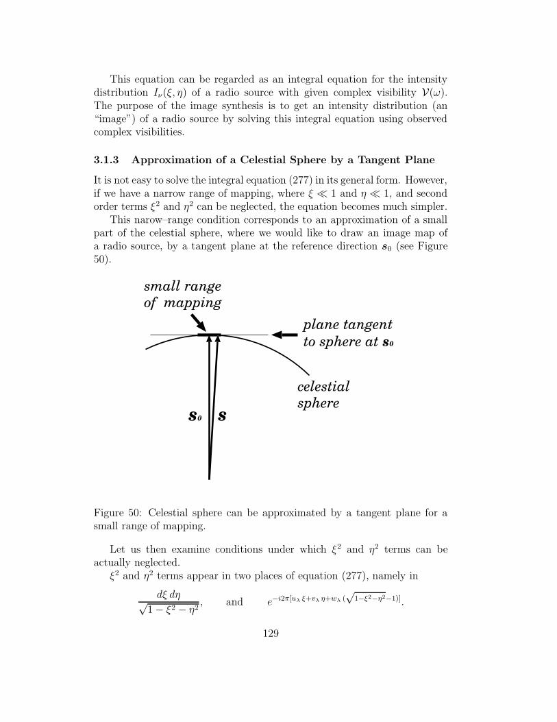
This equation can be regarded as an integral equation for the intensitydistribution Iν(ξ, η) of a radio source with given complex visibility V(ω).The purpose of the image synthesis is to get an intensity distribution (an“image”) of a radio source by solving this integral equation using observedcomplex visibilities.

3.1.3 Approximation of a Celestial Sphere by a Tangent Plane

It is not easy to solve the integral equation (277) in its general form. However,if we have a narrow range of mapping, where ξ 1 and η 1, and secondorder terms ξ2 and η2 can be neglected, the equation becomes much simpler.

This narow–range condition corresponds to an approximation of a smallpart of the celestial sphere, where we would like to draw an image map ofa radio source, by a tangent plane at the reference direction s0 (see Figure50).

s0

celestialsphere

plane tangentto sphere at s0

small rangeof mapping

s

Figure 50: Celestial sphere can be approximated by a tangent plane for asmall range of mapping.

Let us then examine conditions under which ξ2 and η2 terms can beactually neglected.

ξ2 and η2 terms appear in two places of equation (277), namely in

dξ dη√1 − ξ2 − η2

, and e−i2π[uλ ξ+vλ η+wλ (√

1−ξ2−η2−1)].

129

In the first term:dξ dη√

1 − ξ2 − η2, we can neglect ξ2 and η2, provided only

that | ξ | 1 and | η | 1.In the second term, which can be approximated by

e−i2π[uλ ξ + vλ η + wλ (

√

1 − ξ2 − η2 − 1)] ∼= e−i2π[uλ ξ + vλ η −

1

2wλ (ξ2 + η2)]

,(278)

we must be a little careful. Here, ξ2 and η2 terms appear in a phase of aperiodic function, for which only a residue of 2π is meaningful. Therefore,it is not always possible to neglect a term in a phase even when it is muchsmaller than other phase terms. A phase term can be safely neglected onlywhen it is absolutely small as a phase (for example, smaller than 0.1 radian,say). If we require this “ 0.1 radian” condition, then ξ2 and η2 in equation(278) are negligible when

πwλ(ξ2 + η2) 0.1 radian. (279)

Let us now examine how this condition could be satisfied. Let us denote a

(ξ,η)

θf

Dλ

wλ

Figure 51: Length of wλ (left) and a range of mapping (right).

full range of our intended image map (or, range of mapping) as θf . Then,obviously

ξ2 + η2 ≤ (θf2

)2,

(see Figure 51). Therefore, the condition in equation (279) is satisfied if

πwλ(θf2

)2 ≤ 0.1 radian.

Adopting as a maximum value for wλ:

wλmax= Dλ =

D

λ,

130

in view of Figure 51, we see that the condition in equation (279) is readilysatisfied if

π

(

θf2

)2D

λ≤ 0.1, and therefore θ2

f ≤0.4

π

λ

D,

which is approximately equivalent to

θf ≤1

3

√

λ

D. (280)

Thus, the tangent plane approximation, where ξ2 and η2 are neglected, isadequate, if our range of mapping θf satisfies the condition given in equation(280).

It is still left to us to examine whether equation (280) is a realistic con-dition in actual mappings of radio source images.

Angular resolution θr of an interferometric observation is roughly givenby the minimum fringe spacing:

θr ≈λ

D.

Since number of grid points (“pixels”) required for an image mapping isproportional to (θf/θr)

2, a load of numerical processing becomes heavier, asthe range of mapping θf becomes much wider than the angular resolution θr.

Moreover, it is usually meaningless to select a too wide range of mapping,since a radio source, which is much extended than the fringe spacing of aninterferometer θr, tends to be “resolved out” and becomes “invisible” for theinterferometer, as we will see in more detail in later discussions.

Therefore, if we select a range, which is 30 times as large as the angularresolution, as a realistic range of mapping:

θf ≈ 30 × θr ≈ 30 × λ

D,

then, the condition of equation (280) for the tangent–plane approximationbecomes

30λ

D≤ 1

3

√

λ

D, (281)

or√

λ

D≤ 1

90, and, hence,

λ

D≤ 1

8100≈ 0.007 ≈ 25 arcsec. (282)

131

As we saw in Table 2, such a condition on the fringe spacing is generallysatisfied in modern interferometers, except for m–wave or cm–wave CERIarrays of relatively short baselines. In VLBI, as far as our range of mappingis ≤ 30 × (λ/D), we can safely use the tangent–plane approximation. Figure47 gives an example, where the angular resolution is shown as an elliptical“restoring beam” in the right edge.

Figure 52: 15 GHz map of a quasar 3C279 observed with VLBA (Wajimaand Iguchi, private communication in 2005).

Another example of a beautiful VLBI image of a quasar 3C279 observedat 15 GHz with VLBA (Wajima and Iguchi, private communication in 2005)also covers a range of mapping which is smaller than 30 times of the angularresolution (the full width half maximum (FWHM) of an interferometer beamis shown by an ellipse in the left bottom corner).

For typical CERI and VLBI, we have:

• CERI of λ = 1 cm (30 GHz) and D = 2 km:

λ

D= 5 × 10−6 radian = 1 arcsec,

132

1

3

√

λ

D= 7 × 10−4 radian = 140 arcsec.

• VLBI of λ = 1.35 cm (22 GHz) and D = 2300 km:

λ

D= 6.0 × 10−9 radian = 1.2 milliarcsec (mas),

1

3

√

λ

D= 2.6 × 10−5 radian = 5.3 arcsec.

• VLBI of λ = 2.3 mm (129 GHz) and D = 500 km:

λ

D= 4.6 × 10−9 radian = 1.0 milliarcsec (mas),

1

3

√

λ

D= 2.3 × 10−5 radian = 4.7 arcsec.

In all above examples, the condition in equation (281) is well satisfied.Important exceptions, where the tangent–plane approximation is not ap-

plicable, are wide–field mappings of maser sources in massive star–formingregions. They sometimes cover sky ranges of several tens arcseconds, yet in-dividual maser features, of which they consist, are compact at milliarcsecond(mas) level, and thus well detectable with intercontinental VLBIs. In sucha case, the range of mapping θf could be far larger than 30 θr. Therefore,one must properly take into account sphericity of the map surface in suchwide–field mappings.

3.1.4 Interferometer is a Fourier Transformer

Under the tangent plane approximation, equation (277) is reduced to

V(ω) = V(uλ, vλ) =

∞∫

−∞

∞∫

−∞

AN(ξ, η)Iν(ξ, η)e−i2π(uλ ξ+vλ η)dξ dη, (283)

where we reexpressed V(ω) as V(uλ, vλ), stressing dependence of the visibilityon “normalized projected baseline components” uλ and vλ.

Then, it is evident that the complex visibility V(uλ, vλ), as given in equa-tion (283), is a two–dimensional Fourier transform of the source brightnessdistribution Iν(ξ, η) at “spatial frequency” values uλ and vλ.

Consequently, we can regard a radio interferometer as a “Fourier Trans-formation Device”, which yields, at the correlator output, a two–dimensional

133

Fourier component of the source brightness distribution on the sky, at spa-tial frequencies corresponding to two components of the normalized projectedbaseline, uλ and vλ. The Fourier transformation relation described in equa-tion (283) is called “van Cittert–Zernike Theorem”.

Naturally, the source brightness distribution is restored from the mea-sured visibilities by the inverse Fourier transformation:

AN (ξ, η)Iν(ξ, η) =

∞∫

−∞

∞∫

−∞

V(uλ, vλ)ei2π(uλ ξ+vλ η) duλdvλ, (284)

and then by correcting the normalized power pattern of the interferometerAN (ξ, η). This is the basis of the astrophysical imaging of the radio sourcestructure by means of radio interferometry under the tangent plane approxi-mation. This is important also for geodetic and astrometric VLBI, when wecalibrate the effect of the source structure on the measured delay.

Of course, it is impossible to perform a complete inverse Fourier trans-formation, unless a continuous distribution of the visisbility is available overthe whole spatial frequency domain, the uv–plane. Nevertheless, a betterrestoration is achieved, with suitable image processing software, when thevisibilities are sampled at many uλ, vλ points, which nearly homogeneouslycover the uv–plane. It is therefore important to have a good coverage ofuv–plane for radio interferometry observations aimed at astrophysical sourceimaging.

3.2 uv–Coverage

The Earth’s diurnal rotation changes the direction and length of a projectedbaseline of a ground–based interferometer in the uv–plane, and thus helpsus to sample visibilities at different uλ, vλ points. Since the interferometerbaseline rotates around a nearly fixed spin axis of the Earth, the trajectoryof the projected baseline is a circle, if the observed source is located at thecelestial pole. The trajectory is a linear oscillation when the source is at theequator, and is an ellipse, for all other directions in between the celestialequator and the 2 celestial poles. For two stations 1 and 2 on the surfaceof the Earth, we have two baseline vectors with opposite directions D12 andD21 = −D12 connecting these two stations. Therefore, in general, we havetwo point–symmetric arcs of ellipses on the uv–plane for a pair of stations(Figure 53).

Configurations of radio interferometer arrays are designed to achieve goodcoverages of the uv–plane, from the trajectories of projected baselines formedby their antennas.

134

N

E

P

u

v

Figure 53: If we place an end of a baseline vector at the center of the rotatingEarth, by a parallel translation, a tip of the vector draws an ellipse, in general,viewed from a radio source. EW and NS components of the projected baselineare the u and v components. Since we have two vectors of equal lengths andopposite directions which connect two stations, we have two point–symmetricelliptical trajectories.

3.2.1 uv–Trajectories

Figure 54 shows geometry of the diurnal rotation of a baseline vector D.We use an Earth–fixed Cartesian X, Y, Z coordinate system with Z axis

directed towards North Pole, X axis directed towards Greenwich Meridian,and Y axis which completes a right–handed system. Components of thebaseline vector D in this system are denoted by DX , DY , and DZ . Directionof an observed radio source is given by the declination δ and Greenwich hourangle H of the source with respect to this Earth–fixed coordinate system.

First, let us look at the baseline vector from a direction of the North Pole(bottom–left panel of Figure 54). We see two sets of rectangular axes X, Yand S, E in the equatorial plane, which is now perpendicular to our line ofsight. S axis here is chosen along a plane containing both the North Pole axisand the radio source direction, which we call the “PS–plane”. We then con-sider S and E components of the baseline vector D in the equatorial plane.E component is just equal to the u component, i.e. the EW–component ofthe baseline vector viewed from the radio source (top–left panel of Figure54). As for S component of the baseline D, we denote it as DS. Since S,E and X, Y axes are inclined to each other by the Greenwich hour angleH, the u and DS components and DX and DY components of the baselinevector D are related to each other by equations:

u = DX sinH +DY cosH, (285)

135

N

E

P

HDX

DY

DZ

D

u

v

X

Y

N

P

DZ

v

Equa

tori

al p

lane

δ

Z

X

Y

EP

H

DX

DY

u

DS

DS

(Greenwich Meridian)S

S

Figure 54: Geometrical relationship between DX , DY , and DZ components ofa baseline vector D and u, v coordinates. Here, X, Y, Z coordinate system isan Earth–fixed right–handed Cartesian system with Z axis towards the NorthPole P and X axis towards Greenwich Meridian. H and δ are Greenwichhour angle and declination of an observed radio source. The Earth–fixedbaseline vector is shown as viewed from the radio source (top, left), viewedfrom west (top, left), and viewed from the North Pole (bottom).

136

andDS = DX cosH −DY sinH. (286)

Next, when we look at the baseline vector D along the E axis from thewest side (top–right panel of Figure 54), we see equatorial S axis and polarZ axis in the PS–plane, which is now perpendicular to the line of sight. Theradio source direction is offset from the equatorial plane by the declination δ.Therefore, the component of the baseline vector D in an axis perpendicular tothe source direction, which is nothing but the NS–component of the baselinevector viewed from the radio source (top–left panel of Figure 54), i.e. the vcomponent, is related to the DS and DZ components by an equation:

v = −DS sin δ +Dz cos δ. (287)

Combining equations (286) and (287), we obtain

v = −(DX cosH −DY sinH) sin δ +DZ cos δ, (288)

for v component. Equations (285) and (288) allow us to calculate a uv–trajectory of a radio source with varying Greenwich hour angle H.

From equations (285) and (288), we obtain an equation of ellipse:

u2 +(v −DZ cos δ)2

sin2 δ= D2

X +D2Y , (289)

which clearly shows that uv–trajectories are really ellipses.In view of the point symmetry property mentioned above, a set of u and

v:

u = −DX sinH −DY cosH,

v = (DX cosH −DY sinH) sin δ −DZ cos δ, (290)

which satisfies an equation of another ellipse:

u2 +(v +DZ cos δ)2

sin2 δ= D2

X +D2Y , (291)

is also a valid uv–trajectory of the same pair of stations.

When we calculate actual uv–trajectory of a radio source, we must takeinto account that the source can be observed by an interferometer baselineonly when the source is “mutually visible” from two stations of the baseline,i.e. when the source is within lower and upper elevation limits of radio tele-scopes at the two stations. This condition is roughly formulated as follows.

137

P

X

Y

Z

z

H

δ

rs

Figure 55: Zenith distance z of a radio source direction s at a station in adirection r. Also shown is an Earth–fixed Cartesian coordinate system withZ–axis towards the North Pole P and X–axis towards Greenwich Meridian.H and δ are Greenwich hour angle and declination of the source, respectively.

If X, Y , Z coordinates of a station is R = (RX , RY , RZ), and if weapproximate the Earth by a sphere, then a unit vector r oriented towardszenith direction of the station is roughly given by

r =R

R,

whereR =

√

R2X +R2

Y +R2Z .

On the other hand, components of a unit vector s towards a radio source aregiven in the X, Y , Z coordinates by

s = (cos δ cosH, − cos δ sinH, sin δ),

(see Figure 55), where H is the Greenwich hour angle, and δ is the declinationof the source.

Therefore, cosine of the zenith distance z, i.e. the angle between thezenith direction r and the source direction s, is approximately given by

cos z = r · s =RX cos δ cosH − RY cos δ sinH +RZ sin δ

R. (292)

Thus, if upper and lower elevation limits of a radio telescope at a stationare Eu and El, respectively, then the radio source is visible with the telescope

138

whensinEu ≤ cos z ≤ sinEl. (293)

Actual uv–trajectories can be calculated in terms of equations (285),(288), and (290), when the condition of equation (293) is satisfied at bothends of baselines.

Figure 56: uv–trajectories of a combined KVN and VERA arrays, for a sourceat δ = +60.

Figure 56 shows an example of the uv–coverage for the combined VERAand KVN VLBI arrays thus calculated, for a source located at +60 declina-tion.

3.2.2 Synthesized Beams

Let us consider a point source with flux density Sν located at the referencedirection s0 (ξ = 0 and η = 0). In this case, the intensity distribution,which we call here the “true intensity” and denote as I trueν (ξ, η), in order to

139

distinguish it from “synthesized” one to be introduced below, is given by

I trueν (ξ, η) = Sν δ(ξ) δ(η), (294)

where δ(x) is the delta function.For simplicity, we assume that the normalized power pattern of the inter-

ferometer is unity, i.e. AN(ξ, η) = 1, everywhere in our range of mapping.Then, equation (283) gives the complex visibility which is constant at everyuλ, vλ point:

V(uλ, vλ) = Sν = const. (295)

In an actual interferometer array, we can sample the complex visibilityonly along uv–trajectories. Therefore, the “synthesized intensity distribu-tion” calculated by equation (284):

Isyntν (ξ, η) = Sν

∞∫

−∞

∞∫

−∞

ei2π(uλξ+vλη)du dv∣

∣

∣

along uv, (296)

does not reproduce the point but yields some extended distribution. This“response of a synthesis interferometer array to a point source” is called the“synthesized beam” or the “dirty beam” of the array. This is analogousto the beam formation of a single dish antenna with a strange “apertureillumination” along elliptical arcs.

If we approximate the two–dimensional integration by a summation onmeshes, equation (296) is reduced to

Isyntν (ξ, η) = Sν

∑

u

∑

v

ei2π(uλξ+vλη)∆uλ ∆vλ∣

∣

∣

along uv

= Sν

∑

u

∑

v

[ei2π(uλξ+vλη) + e−i2π(uλξ+vλη)]∆uλ ∆vλ∣

∣

∣

along uv1

= 2Sν

∑

u

∑

v

cos(2π[uλξ + vλη])∆uλ ∆vλ∣

∣

∣

along uv1, (297)

where “along uv” means summation along uv–trajectories composed of point–symmetric elliptical arcs given in both equations (289) and (291), whereas“along uv1” means summation along uv–trajectories given by equation (289)only. We can further replace the two–dimensional summation on the uv–plane by a one–dimensional summation along the elliptical uv–trajectorieswith equal intervals of Greenwich hour angle ∆H. Since an interval in Green-wich hour angle ∆H corresponds to a length interval in the uv–plane

√

√

√

√

(

duλdH

)2

+

(

dvλdH

)2

∆H,

140

we obtain from equation (297)

Isyntν (ξ, η) ∝∑

H

cos(2π[uλ(H)ξ+vλ(H)η])

√

√

√

√

(

duλdH

)2

+

(

dvλdH

)2

∆H∣

∣

∣

along uv1.

(298)

Synthesized Beam of KVN+VERA Dec = +60 deg

Freq = 22.0 GHz

-2.5-2-1.5-1-0.500.511.522.5

RA offset (milliarcsec) -2.5-2

-1.5-1

-0.50

0.51

1.52

2.5

Dec offset (milliarcsec)

-0.2

0

0.2

0.4

0.6

0.8

1

normalized beam

Figure 57: Normalized synthesized beam of the combined KVN and VERAVLBI arrays for a radio source at +60 declination with observing frequency22 GHz.

uλ, vλ and their derivatives with respect toH in equation (298) are readilycalculated for a radio source with declination δ from equations (285) and(288), namely we have

uλ =DX sinH +DY cosH

λ, (299)

vλ = −DX cosH −DY sinH

λsin δ +

DZ

λcos δ, (300)

andduλdH

=DX cosH −DY sinH

λ, (301)

dvλdH

=DX sinH +DY cosH

λsin δ. (302)

141

Calculating these quantities with varying H while the source is mutuallyvisible at two ends of baselines, inserting them into equation (298), anddividing the results by a maximum value, we obtain the synthesized beamnormalized by its maximum value:

Isyntν (ξ, η)

Isyntν max

.

Figure 57 shows an example of the normalized synthesized beam for thecombined KVN and VERA VLBI arrays for a radio source located at +60

declination observed at 22 GHz.

3.3 Correlated Flux Density of a Source with Gaussian

Intensity (Brightness) Distribution

How is the correlated flux density related to the size of an observed radiosource? Let us consider this problem for a simple case, when the source hasa circular Gaussian intensity (brightness) distribution (Figure 58):

Iν(ξ, η) =STν

πΘ2s

e− ξ2+η2

Θ2s , (303)

where STνis the total flux density (note that

∞∫

−∞

∞∫

−∞

e− ξ2+η2

Θ2s dξ dη = πΘ2

s ),

Iν(ρ)

ρ

Θ0

Figure 58: Circular Gaussian intensity distribution Iν(ρ) with ρ =√ξ2 + η2.

and Θs is a parameter characterizing the source size. This parameter Θs isrelated to the half–power width of the Gaussian distribution Θ0 by a formula:

Θs =Θ0

2√

ln 2∼= 0.60Θ0. (304)

142

Then, in view of equation (283), the complex visibility of the source isgiven by

V(uλ, vλ) =STν

πΘ2s

∞∫

−∞

∞∫

−∞

e− ξ2 + η2

Θ2s e−i2π(uλ ξ+vλ η) dξ dη

= STνe−π

2 Θ2s (u2

λ+ v2

λ) = STν

e−[πΘs (D cos θλ )]

2

(305)

(see Figure 59 for geometry of the projected baseline), where we took AN(ξ, η) ∼=1, for simplicity, assuming that the source is observed at beam centers of an-tennas. In deriving equation (305), we used an integration formula:

∞∫

−∞

e−x2 − i a x dx =

√π e−

a2

4 .

s0

D

uλ

vλ

θ

D cos θλ

Figure 59: Projected baseline length:√

u2λ + v2

λ = D cos θλ

.

Thus, for a source with the circular Gaussian intensity distribution, wehave

• correlated flux density = | V(uλ, vλ) | = STνe−[πΘs (D cos θ

λ )]2

,• visibility phase = 0.This means that the correlated flux density | V(uλ, vλ | is reduced to the

half of the total flux density STνwhen

[

πΘs(D cos θ

λ)

]2

= ln 2, (306)

143

or, in view of equation (304), when the half–power width of the source dis-tribution Θ0 is equal to

Θ0 =2 ln 2

π

λ

D cos θ∼= 0.44

λ

D cos θ. (307)

correlated flux correlated flux

0 0

STν STν

Θ0 D cos θ / λ

Θ0D cos θ

curve for given baseline curve for given source size

point source

0.44 λ/Dcosθ 0.44 /Θ0

Figure 60: Correlated flux density of a source with Gaussian intensity dis-tribution, as a function of the source size (left), and as a function of theprojected baseline length (right).

Figure 60 shows the correlated flux density of the source, with a circularGaussian intensity distribution, as a function of the half–power width Θ0 ofthe source brightness distribution, assuming a fixed baseline length D (leftpanel); and as a function of the projected baseline length normalized by thewave length, D cos θ/λ, assuming a fixed source size (right panel), accordingto equation (305). This simple example shows that the source appears weakto an interferometer, or “resolved out”, when its size becomes comparablewith or larger than the fringe spacing λ/(D cos θ). In other words, inter-ferometers are sensitive to the sources with angular sizes comparable to orsmaller than their fringe spacings.

It is usual practice in VLBI to infer the size of a source by measuring itscorrelated flux densities at different projected baseline lengths, and fittingthe results to a Gaussian model, as shown in the right panel of Figure 60.Figure 61 shows an example (Wajima and Iguchi, private communication in2005).

144

Figure 61: Visibility amplitude (top) and phase (bottom) versus uv–distancealong a position angle (PA) 60 plot of a quasar 3C279 observed with VLBAat 15 GHz (Wajima and Iguchi, private communication in 2005). Visibilityamplitude (top) decreases with uv–distance (projected baseline length) in arange from 0 to 70×106 λ, similarly to the curve in the right panel of Figure60. However, visibility amplitude becomes almost flat in uv–distance rangefrom 70 × 106 to 400 × 106 λ, showing existence of a compact componentwhich is not resolved even on the longest baseline 400 × 106 λ ' 8000 km.This Figure can be compared with an image map of the same source shownin Figure 52.

145

Figure 62: VLBI can observe very bright, compact objects only.

3.4 What Can VLBI Observe?

The above discussions show that a VLBI (or an interferometer, in general),with baseline length D and observing wavelength λ, can detect only compactsources with characteristic angular diameters Θ0 comparable to or smallerthan λ/D, i.e.,

Θ0 ≤λ

D.

If the brightness temperature of a source is TB, then the intensity Iν andthe flux density Sν are given by:

Iν =2kTBλ2

, and Sν =2kTBλ2

πΘ20

4≤ πkTB

2D2,

where k = 1.381× 10−23 JK−1 is the Boltzmann constant. Note that the lastexpression does not depend on the wavelength.

Now, if the minimum detectable flux density by VLBI is Sνmin, we canimpose a lower limit to the brightness temperature, TBmin, for the detectablesource:

TBmin ∼= 2D2

πkSνmin. (308)

If D = 2300 km and Sνmin = 0.02 Jy, then TBmin ∼= 5 × 107 K (!).

146

Such a high lower limit of the brightness temperature precludes detectionof almost all thermal sources, such as stars and molecular clouds with VLBI,leaving only very bright, compact non–thermal sources, e.g., AGNs, masers,and pulsars (see Figure 62), to be detected.

4 Signal–to–Noise Ratio in Radio Interfer-

ometry

So far, we approximated the result R of the multiplication and integrationin a correlator by the cross–correlation RU1U2(0) of the voltage signals U1(t)and U2(t) at input points of the correlator. In view of the ergodicity, thisapproximation should be good enough when the integration time is suffi-ciently long. Also, one can prove that the mathematical expectation of R isequal to RU1U2(0), if U1(t) and U2(t) are jointly stationary random processes.However, the actual correlator output, with some limited integration time, isinevitably accompanied with thermal noise fluctuations. Therefore, we havesome finite signal–to–noise–ratio in the correlator output, which determinesdetectability of the radio source signal, i.e. the sensitivity (Figure 63).

t

t

signal

signal

Figure 63: Signal–to–noise ratio of the correlator output determines the sen-sitivity of an interferometer.

We will see in the followings that a statistical theory of the dispersion of

147

the time–averaged product of random processes gives a theoretical expressionfor the signal–to–noise ratio S/N of the correlator output.

4.1 Statistical Model of a Correlator Output

4.1.1 Signal + Noise Inputs to a Correlator

Let us consider that the voltages from two antennas U1(t) and U2(t), whichare fed to input points of a correlator, consist of signals V1(t), V2(t) and

multiplier

integrator

from antenna 1 from antenna 2

.

U2=V2+N2U1=V1+N1

RV1V2 + Noise

Figure 64: Input voltages to a correlator consist of signals and noises.

noises N1(t), N2(t) (see Figure 64):

U1(t) = V1(t) +N1(t),

U2(t) = U2(t) +N2(t). (309)

We assume that the delay tracking and fringe stopping were already success-fully applied to the voltages U1(t) and U2(t), so that we can integrade themultiplier output for an appropriate interval of time without losing signalpower.

4.1.2 Integration of the Multiplier Output

If we denote an instantaneous output of the multiplier as y(t):

y(t) = U1(t)U2(t), (310)

an output of the integrator (i.e., correlator output) z(t) is related to the inputy(t) by a linear system of time averaging with an impulse response a(t):

z(t) = y(t) ∗ a(t) =

∞∫

−∞

y(t′)a(t− t′) dt′, (311)

148

where symbol ‘∗’ stands for a convolution, as before.If an input y(t) is a constant y in time, the time averaging result must be

equal to the constant y. Therefore, the impulse response a(t) must satisfy:

∞∫

−∞

a(t) dt = 1. (312)

For example, if we take a simple running mean:

z(t) =1

2T

t+T∫

t−T

y(t′) dt′, (313)

then the impulse response a(t) is given by

a(t) =

12T

for − T ≤ t ≤ T,

0 otherwise.

4.1.3 Statistical Expectation of the Correlator Output

We assume that the noise components from two antennas are not correlatedwith each other, and are not correlated with signal components, either. Then,we have

〈N1(t)N2(t)〉 = 0, 〈Vi(t)Nj(t)〉 = 0 for i = 1, 2 and j = 1, 2, (314)

where 〈 〉 stands for the ensemble average, as before. From equation (314),we obtain

〈y(t)〉 = 〈U1 U2〉 = 〈[V1(t) +N1(t)] [V2(t) +N2(t)]〉 = 〈V1(t)V2(t)〉. (315)

In next subsection, we will see that the multiplier output y(t) = U1(t)U2(t)is a stationary random process, provided that U1(t) and U2(t) are jointly sta-tionary random processes obeying the zero–mean jointly normal (or Gaus-sian) probability density. If so,

〈y(t)〉 = const,

and, therefore,

〈z(t)〉 =

∞∫

−∞

〈y(t′)〉a(t− t′) dt′ = 〈y(t)〉∞∫

−∞

a(t− t′)dt′ = 〈y(t)〉, (316)

in view of equation (312). Equations (315) and (316) show that the statisticalexpectation of the correlator output in radio interferometry does not containsystem–noise contribution unlike in the single–dish radio telescope case.

149

4.1.4 Dispersion of the Correlator Output

As we saw in the discussion of the correlation ergodicity in Subsection 1.2.4,a correlator output z(t) with finite integration time should be associated withnoise–induced fluctuations around the expectation:

z(t) = 〈z(t)〉 + noise = 〈V1(t)V2(t)〉 + noise. (317)

This fluctuation determines detection limit of radio sources as illustrated inFigure 64.

The magnitude of this fluctuation can be estimated by the dispersion σ2z

of the correlator output z(t), as we saw in the discussion of the correlationergotic processes. The dispersion is given by

σ2z = 〈[z(t) − 〈z(t)〉]2〉

= 〈[z2(t) − 2z(t) 〈z(t)〉 + 〈z(t)〉2]〉= 〈z2(t)〉 − 〈z(t)〉2, (318)

and, therefore, the standard deviation is given by

σz =√

〈z2(t)〉 − 〈z(t)〉2. (319)

This is a measure of strength of the noise in the correlator output.On the other hand, strength of the signal in the correlator output is given

by the theoretical expressions of the fringe amplitude AU and AL shown inequations (260) and (261) for USB and LSB receptions, respectively, for acontinuum spectrum source.

Therefore, signal–to–noise ratio SNR for a continuum spectrum sourceis given by

SNR =Aσz, (320)

where A is either AU or AL, depending on a choice of the single sidebandactually received.

In following subsections, we will calculate the standard deviation of thecorrelator output σz, in order to get an explicit expression of the signal–to–noise ratio in terms of physical parameters characterizing the radio sourceand antenna–receiving systems.

4.2 Useful Formulae Related to the Correlator Output

In calculating the standard deviation of the correlator output σz, we will usefollowing formulae relevant to the present problem.

150

4.2.1 Fourth Order Moment Relation

Let x1, x2, · · ·, xn are zero–mean random variables obeying to the jointlynormal (or Gaussian) probability density given in equation (29):

f(x1, · · · , xn) =1

√

(2π)n∆e− 1

2

n∑

i=1

n∑

j=1

xi C−1ij

xj

, (321)

where expectation ηi of the random variable xi figuring in equation (29) iszero by assumption for all i = 1, 2, · · · , n; Cij ≡ 〈xi xj〉 is a covariance matrix,C−1ij is its inverse matrix, and ∆ ≡ detCij is its determinant. In general,

we denote an inverse matrix by a symbol ( )−1 and a determinant by det ( ).A very useful formula is known for such jointly normal random variables

xi (i = 1, · · · , n):

〈xi xj xk xl〉 = 〈xi xj〉 〈xk xl〉 + 〈xi xk〉 〈xj xl〉 + 〈xi xl〉 〈xj xk〉, (322)

which says that a fourth order statistical moment (a term “n–th order sta-tistical moment” is used here to denote a statistical expectation of a productof n random variables) 〈xi xj xk xl〉 is decomposed as a sum of products ofsecond order statistical moment (correlations) 〈xi xj〉.

Proof :

1. Let us reformulate equation (321), using matrix notation of a row vectorX and its transpose XT :

X =

x1

x2

...

xn

, and XT = (x1 x2 · · · xn),

where ( )T denotes a transpose matrix. Then we have

f(X) =1

√

(2π)n∆e−

12XT C−1X , (323)

where C is the covariance matrix which is a positive–definite symmetricmatrix with Cij = 〈xi xj〉 as ij–element.

151

2. Fourier transform of a probability density is called “characteristic func-tion”. A characteristic function F (Ω) of the joint probability densityf(X) in equation (323), where Ω is a row vector of angular frequenciesΩT = (ω1 ω2 · · · ωn), is given by

F (Ω) =

∞∫

−∞

· · ·∞∫

−∞

f(X) e−iΩT X dx1 · · · dxn = 〈e−iΩT X〉

=1

√

(2π)n∆

∞∫

−∞

· · ·∞∫

−∞

e−12XT C−1 X − iΩT X dx1 · · · dxn.

(324)

3. According to the linear algebra, a symmetric matrix can be diagonal-ized by a suitable orthogonal transformation. So, let T be an orthogonalmatrix, which diagonalizes the symmetric matrix C−1:

T T C−1 T =

λ1 0 · · · 0

0 λ2 · · · 0...

.... . .

...

0 0 · · · λn

, (325)

where λ1, λ2, · · · , λn are eigen values of the matrix C−1.

Since T is an orthogonal matrix, by definition we have

T T T = T T T = I, T−1 = T T , det T = 1, (326)

where I is a unit matrix:

I =

1 0 · · · 0

0 1 · · · 0...

.... . .

...

0 0 · · · 1

,

and, therefore,

T T C T = (T T C−1 T )−1 =

λ−11 0 · · · 0

0 λ−12 · · · 0

......

. . ....

0 0 · · · λ−1n

, (327)

152

and

∆ = det C = det T T det C det T = det(T T C T ) =1

λ1 λ2 · · · λn.

(328)

4. If we introduce a new row vector Y :

Y T = (y1 y2 · · · yn),

which is obtained by an orthogonal transformation of X with T :

Y = T T X,

then we have

X = T Y,∂xi∂yj

= Tij,∂(x1 x2 · · · xn)∂(y1 y2 · · · yn)

= det T = 1,

XT C−1X = Y T T T C−1 T Y =n∑

j=1

λj y2j ,

ΩT X = ΩT T Y =n∑

i=1

n∑

j=1

ωi Tij yj. (329)

Therefore, the characteristic function F (Ω) given in equation (324) isreduced to

F (Ω) =1

√

(2π)n∆

∞∫

−∞

· · ·∞∫

−∞

e

−1

2

n∑

j=1

λj y2j − i

n∑

i=1

n∑

j=1

ωi Tij yjdy1 · · · dyn.

(330)If we further introduce new variables:

zj =

√

λj2yj (j = 1, · · · , n),

then we have

F (Ω) =1

√

(2π)n∆

∞∫

−∞

· · ·∞∫

−∞

e

−n∑

j=1

(z2j + i

n∑

i=1

ωi Tij

√

2

λjzj)√ 2n

λ1 · · ·λndz1 · · · dzn,

=1√πn

∞∫

−∞

· · ·∞∫

−∞

e

−n∑

j=1

(z2j + i

n∑

i=1

ωi Tij

√

2

λjzj)

dz1 · · · dzn.

(331)

153

5. Applying the integration formula:∞∫

−∞

e−x2 − i a x dx =

√π e−

a2

4 ,

we reduce equation (331) to

F (Ω) = e

−1

4

n∑

j=1

(

n∑

i=1

ωi Tij

√

2

λj

)2

= e

−1

2

n∑

i=1

n∑

j=1

n∑

k=1

ωi Tij1

λjTkj ωk

= e−12

ΩT C Ω. (332)

6. From equations (324) and (332), we have

〈e−iΩT X〉 = e−12

ΩT C Ω. (333)

Expanding exponential functions in both sides of this equation into theTaylor series, we have

〈e−iΩT X〉 = 1 − 1

2!〈(ΩT X)2〉 + i

1

3!〈(ΩT X)3〉 +

1

4!〈(ΩT X)4〉 − · · · ,

e−12

ΩT C Ω = 1 − 1

2ΩT C Ω +

1

2!(1

2ΩT C Ω)2 − · · · . (334)

Terms with fourth order of ωi ’s in the above equations are

1

4!〈(ΩT X)4〉 =

1

4!

n∑

i=1

n∑

j=1

n∑

k=1

n∑

l=1

〈xi xj xk xl〉ωi ωj ωk ωl, (335)

and

1

2!(1

2ΩT C Ω)2 =

1

2!

1

4

n∑

i=1

n∑

j=1

n∑

k=1

n∑

l=1

Cij Ckl ωi ωj ωk ωl

=1

4!

n∑

i=1

n∑

j=1

n∑

k=1

n∑

l=1

(Cij Ckl + Cik Cjl + Cil Cjk)ωi ωj ωk ωl, (336)

respectively. Right hand sides of equations (335) and (336) are equalto each other in view of equation (333). Consequently, coefficients ofωi ωj ωk ωl in these equations, i.e., 〈xi xj xk xl〉 and Cij Ckl + Cik Cjl +Cil Cjk, must be equal to each other, too, since both of them are in-variant in any substitution of i, j, k, l. Thus, we have

〈xi xj xk xl〉 = Cij Ckl + Cik Cjl + Cil Cjk. (337)

Since Cij = 〈xi xj〉, this completes the proof of equation (322).

154

4.2.2 Multiplier Output as a Stationary Random Process

If two voltage inputs U1(t) and U2(t) of a correlator are jointly station-ary processes and if they obey the zero–mean jointly normal (or Gaus-sian) probability density such as given in equation (321), then their producty(t) = U1(t)U2(t) is also a stationary random process.

Proof :

1. Expectation of y(t) is a constant in time. In fact,

〈y(t)〉 = 〈U1(t)U2(t)〉 = RU1U2(0), (338)

where RU1U2(τ) = 〈U1(t)U2(t − τ)〉 is a cross–correlation of jointlystationary random processes U1(t) and U2(t), and, therefore, 〈y(t)〉 doesnot depend on time t.

2. Autocorrelation of y(t) is a function of time difference only. In fact, inview of equation (322), we have

〈y(t) y(t− τ)〉 = 〈U1(t)U2(t)U1(t− τ)U2(t− τ)〉= 〈U1(t)U2(t)〉 〈U1(t− τ)U2(t− τ)〉+〈U1(t)U1(t− τ)〉 〈U2(t)U2(t− τ)〉+〈U1(t)U2(t− τ)〉 〈U2(t)U1(t− τ)〉

= R2U1U2

(0) +RU1U1(τ)RU2U2(τ) +RU1U2(τ)RU1U2(−τ),(339)

where RU1U1(τ) = 〈U1(t)U1(t − τ)〉 and RU2U2(τ) = 〈U2(t)U2(t − τ)〉are autocorrelations of input voltages U1(t) and U2(t). This equationshows that 〈y(t) y(t− τ)〉 is a function of time difference τ only.

Thus, we proved that the multiplier output y(t) is a stationary random pro-cess.

Since the integrator output (i.e., correlator output) z(t) is an output of alinear system of time averaging, given in equation (311), with the input y(t)which was shown to be a stationary random process, we conclude that z(t)is also a stationary random process.

Hereafter, we will denote autocorrelations of the multiplier output y(t)and the integrator output z(t) as functions of time difference τ :

Ryy(τ) = 〈y(t) y(t− τ)〉,Rzz(τ) = 〈z(t) z(t− τ)〉. (340)

155

4.2.3 Time Averaging Operator

Since the multiplier output y(t) and the integrator output z(t) are relatedto each other through the impulse response a(t) of the operator of timeaveraging, as shown in equation (311):

z(t) = y(t) ∗ a(t),their autocorrelations are related to each other as:

Rzz(τ) = Ryy(τ) ∗ a(τ) ∗ a(−τ), (341)

in view of equation (42).Therefore, if we denote power spectra of y(t) and z(t) as Syy(ω) and

Szz(ω):

Syy(ω) ⇔ Ryy(τ),

Szz(ω) ⇔ Rzz(τ),

where symbol ⇔ stands for a Fourier transformation pair, and introduce asystem function A(ω) of a(t):

A(ω) ⇔ a(t),

then we have, in view of equation (72),

Szz(ω) = Syy(ω) | A(ω) |2 . (342)

Since

A(ω) =

∞∫

−∞

a(t) e−iωtdt,

and, from equation (312),∞∫

−∞

a(t) dt = 1,

the system function A(ω) must always satisfy an equation:

A(0) = 1. (343)

Note that, for the case of a simple running mean, the system functiontakes the sinc function form:

A(ω) =1

2T

T∫

−T

e−iωtdt =sin(ωT )

ω T. (344)

In general, A(ω) can be regarded as a low–pass filter with a narrow pass-band of about ±2π/T , as evident from the above simple case. If the integraltime T is 1 s, for example, the passband is as narrow as ±1 Hz.

156

4.2.4 Power Spectrum of Multiplier Output

Let us now describe the power spectrum of the multiplier output Syy(ω)through power and cross–power spectra of voltages, which are the inputs toour correlator.

From equations (339) and (340), we have

Ryy(τ) = R2U1U2

(0) +RU1U1(τ)RU2U2(τ) +RU1U2(τ)RU1U2(−τ). (345)

Therefore, Fourier transformation of this equation gives us the power spec-trum Syy(ω). Using convolution theorem in Fourier transformation, given inequation (67), for products of functions of τ , we obtain

Syy(ω) =

∞∫

−∞

Ryy(τ)e−iωτdτ

= 2πR2U1U2

(0) δ(ω)

+1

2πSU1U1(ω) ∗ SU2U2(ω) +

1

2πSU1U2(ω) ∗ S∗

U1U2(ω), (346)

where δ(ω) is the delta function of angular frequency ω, and SU1U1(ω),SU2U2(ω), and SU1U2(ω) are power and cross–power spectra of input voltages:

SU1U1(ω) ⇔ RU1U1(τ),

SU2U2(ω) ⇔ RU2U2(τ),

SU1U2(ω) ⇔ RU1U2(τ).

Here we used a relation:

∞∫

−∞

e−iωτdτ = 2πδ(ω),

which was given in equation (65), and for Fourier transform of a real functionRU1U2(−τ):

∞∫

−∞

RU1U2(−τ)e−iωτdτ =

∞∫

−∞

RU1U2(τ)eiωτdτ

=

∞∫

−∞

RU1U2(τ)e−iωτdτ

∗

= S∗U1U2

(ω).

157

4.2.5 Power and Cross–Power Spectra of Input Voltages

Power and cross–power spectra of input voltages figuring in equation (346)can be described as follows.

Assuming, as before, that signal and noise are not correlated with eachother, and noises from different antennas are not correlated, either, we ex-press autocorrelations and cross–correlation of input voltages U1(t) and U2(t)in terms of signal (V ) and noise (N) components:

RU1U1(τ) = RV1V1(τ) +RN1N1(τ),

RU2U2(τ) = RV2V2(τ) +RN2N2(τ),

RU1U2(τ) = RV1V2(τ), (347)

where

RV1V1(τ) = 〈V1(t)V1(t− τ)〉,RV2V2(τ) = 〈V2(t)V2(t− τ)〉,RV1V2(τ) = 〈V1(t)V2(t− τ)〉,

are auto– and cross–correlations of signal voltages V1(t) and V2(t), while

RN1N1(τ) = 〈N1(t)N1(t− τ)〉,RN2N2(τ) = 〈N2(t)N2(t− τ)〉,

are autocorrelations of noise voltages N1(t) and N2(t).Therefore, the power and cross–power spectra are obtained by Fourier

transformation of equations (347) as

SU1U1(ω) = SV1V1(ω) + SN1N1(ω),

SU2U2(ω) = SV2V2(ω) + SN2N2(ω),

SU1U2(ω) = SV1V2(ω), (348)

where

SV1V1(ω) ⇔ RV1V1(τ),

SV2V2(ω) ⇔ RV2V2(τ),

SV1V2(ω) ⇔ RV1V2(τ),

are power and cross–power spectra of signal voltages, while

SN1N1(ω) ⇔ RN1N1(τ),

SN2N2(ω) ⇔ RN2N2(τ),

are power spectra of noise voltages.

158

4.2.6 Antenna Temperature and System Noise Temperature

We saw in equation (169), that a power spectrum Svivi(ω) of a received signal

voltage vi(t) (i = 1, 2) at RF band, which is just received by i–th antenna,and has not yet gone through a receiving system, is given in terms of effectiveflux density Sν of an observed source and efective aperture of i–th antennaAei

by

Svivi(ω) =

1

4Aei

Sν (i = 1, 2).

Since the effective flux density and the antenna temperature TAi(ω), char-

acterizing a received power from a radio source per unit bandwidth, are re-lated to each other by an equation:

k TAi(ω) =

1

2Aei

Sν,

as we saw in Chapter 2, where k = 1.381 × 10−23 JK−1 is Boltzmann’s con-stant, the power spectrum of the received signal voltage is described throughthe antenna temperature as:

Svivi(ω) =

1

2k TAi

(ω) (i = 1, 2). (349)

Since the frequency conversion preserves the power spectrum of the re-ceived signal voltage, we can easily derive from equation (349) a power spec-trum SViVi

(ω) of an IF signal voltage Vi(t) at an input of a correlator. Indeed,if we denote the system function of the receiving system as Hi(ω), as givenin equation (195), and if we assume for definiteness upper sideband (USB)reception, we have

SViVi(ω) =

1

2k TAi

(ωLO + ω) | Hi(ω) |2 (for ω ≥ 0, i = 1, 2), (350)

where ω is frequency in IF band and ωLO is local oscillator frequency of thefrquency conversion. Here we showed only positive frequency side of thepower spectrum, which is an essentially even function of frequency.

On the other hand, the noise component is described through the in-put equivalent system noise temperature TSi

(ω), which is supposed to passthrough the same receiving system as the radio source signal does. Thus, inthe USB reception and in the positive frequency range, we have

SNiNi(ω) =

1

2k TSi

(ωLO + ω) | Hi(ω) |2 (for ω ≥ 0, i = 1, 2). (351)

159

Therefore, from equations (348), (350), and (351), the power spectrum ofthe input voltage Ui(t) is given by

SUiUi(ω) =

1

2k [TAi

(ωLO+ω)+TSi(ωLO+ω)] | Hi(ω) |2 (for ω ≥ 0, i = 1, 2),

(352)in the USB reception and in the positive frequency range.

The cross–power spectrum of two input signal voltages Vi(t), (i = 1, 2) af-ter delay tracking and fringe stopping is given in equation (242), for the caseof the USB reception and in the positive frequency range of the Hermitiansymmetric cross–power spectrum. Therefore, taking into account also equa-tion (348), the cross–power spectrum of the input voltages Ui(t), (i = 1, 2)in the positive frequency range (ω ≥ 0) is given by

SU1U2(ω) = SV1V2(ω) =1

4A0 e

−i(φLO1−φLO2) V(ωLO + ω)H1(ω)H∗2(ω), (353)

where A0 is geometric mean of effective apertures of antennas, φLO1−φLO2 isdifference of initial phases of local oscillators, and we put ∆τg = 0 in equation(242), assuming complete delay tracking and fringe stopping.

In a simple case of a point–like radio source with normalized powerpattern of the interferometer AN (σ) = 1 at centers of antenna beams,the complex visibility of the source is real and equal to its flux density,V(ωLO + ω) = Sν, as given in equation (295), and, therefore,

1

4A0 V(ωLO + ω) =

1

4

√

Ae1Ae2 Sν =1

2k√

TA1(ωLO + ω)TA2(ωLO + ω).

(354)In this case, we have, in ω ≥ 0

SU1U2(ω) =1

2k√

TA1(ωLO + ω)TA2(ωLO + ω) e−i(φLO1−φLO2) H1(ω)H∗2(ω).

(355)

4.3 Sensitibity of a Radio Interferometer

4.3.1 Standard Deviation Due to the Noise

Now we are ready to calculate the standard deviation σz of the correlatoroutput z(t) in equation (319), and then the signal–to–noise ratio in equation(320).

In equation (319):

σz =√

〈z2(t)〉 − 〈z(t)〉2,

160

the first term 〈z2(t)〉 in square root is given by inverse Fourier transformationat τ = 0 of the power spectrum Szz(ω), which is related to Syy(ω) given inequation (346) through equation (342). Therefore, we have

〈z2(t)〉 =1

2π

∞∫

−∞

Szz(ω) dω =1

2π

∞∫

−∞

Syy(ω) | A(ω) |2 dω

=1

2π

∞∫

−∞

[

2πR2U1U2

(0) δ(ω)

+1

2πSU1U1(ω) ∗ SU2U2(ω) +

1

2πSU1U2(ω) ∗ S∗

U1U2(ω)

]

| A(ω) |2 dω= R2

U1U2(0)

+1

(2π)2

∞∫

−∞

[

SU1U1(ω) ∗ SU2U2(ω) + SU1U2(ω) ∗ S∗U1U2

(ω)]

| A(ω) |2 dω,

(356)

where A(ω) is the system function of time averaging, and we used equation(343) for deriving the first term. On the other hand, second term 〈z(t)〉2 isequal to R2

U1U2(0), since, in view of equations (317) and (338), we have

〈z(t)〉 = RU1U2(0).

Therefore, the first term of the right hand side of equation (356) is compen-sated by 〈z(t)〉2, and hence we have

σ2z =

1

(2π)2

∞∫

−∞

[

SU1U1(ω) ∗ SU2U2(ω) + SU1U2(ω) ∗ S∗U1U2

(ω)]

| A(ω) |2 dω.

(357)If we use explicit forms of convolution integrals, equation (357) is reduced to

σ2z =

1

(2π)2

∞∫

−∞

∞∫

−∞

[SU1U1(ω − ω′)SU2U2(ω′)

+SU1U2(ω − ω′)S∗U1U2

(ω′)]

| A(ω) |2 dω′ dω. (358)

Since A(ω) is a very narrow–band low–pass filter around ω = 0, as wesaw earlier, SU1U1(ω−ω′) and SU1U2(ω−ω′) can be replaced by SU1U1(−ω′) =SU1U1(ω

′) and SU1U2(−ω′) = S∗U1U2

(ω′), and we can take them out of theintegration with respect to ω. Thus we obtain,

σ2z =

1

(2π)2

∞∫

−∞

[

SU1U1(ω′)SU2U2(ω

′) + S∗U1U2

(ω′)S∗U1U2

(ω′)]

dω′

∞∫

−∞

| A(ω) |2 dω.

(359)

161

Taking into account that SU1U1(ω′) is an even, and SU1U2(ω

′) is a Hermitiansymmetric, functions, we can further reduce equation (359) to

σ2z =

1

2π2

∞∫

0

SU1U1(ω′)SU2U2(ω

′)

+< [SU1U2(ω′)SU1U2(ω

′)] dω′

∞∫

−∞

| A(ω) |2 dω. (360)

Now, assuming the USB reception, for definiteness, we apply equations(352) and (355) for spectra in positive frequency range (ω ≥ 0) of inputvoltages to obtain

σ2z =

k2

8π2

∞∫

0

(TA1 + TS1) (TA2 + TS2) | H1(ω′) |2| H2(ω

′) |2

+< [(TA1 TA2) e−2i(φLO1

−φLO2)H1(ω

′)H∗2(ω

′)H1(ω′)H∗

2 (ω′)]

dω′

×∞∫

−∞

| A(ω) |2 dω, (361)

where we omitted argument ωLO + ω in TAiand TSi

(i = 1, 2) for simplicity.Since, in actual observations of most of radio sources, antenna tempera-

tures are much smaller than system noise temperatures: TAi TSi

(i = 1, 2),we ignore terms with TAi

, compared with terms with TSi(i = 1, 2). Then,

assuming a flat noise spectrum, we obtain an equation:

σ2z =

k2 TS1 TS2

8π2

∞∫

0

| H1(ω′) |2 | H2(ω

′) |2 dω′

∞∫

−∞

| A(ω) |2 dω, (362)

which describes the dispersion of noise fluctuations in the correlator output.

4.3.2 Signal in the Correlator Output

Now, if we assume a continuum spectrum source and USB reception, thesignal in the correlator output is given by the theoretical expression of thefringe amplitude A in equation (260):

A = A0 | V | | B12 |,

where A0 is the geometric mean of effective apertures of element antennas,| V | is the visibility amplitude, and | B12 | is the amplitude of the bandwidth

162

pattern defined in equation (254). In the simple case of the point–like source,for which the visibility V is equal to the flux density Sν, we have

A0 | V |=√

Ae1 Ae2 Sν = 2 k√

TA1 TA2 ,

and, therefore,

A = 2 k√

TA1 TA2 | B12 | . (363)

4.3.3 Signal–to–Noise Ratio of the Correlator Output

Consequently, the signal–to–noise ratio is given by

SNR =Aσz

= 8π

√

TA1 TA2

TS1 TS2

| B12 |√

2∞∫

0| H1(ω′) |2 | H2(ω′) |2 dω′

1√

∞∫

−∞| A(ω) |2 dω

.

(364)

Let us first assume simple rectangular filters which are given in positivefrequency range (ω ≥ 0) by:

| Hi(ω) |2=

Gi if ωI − ∆ω2

≤ ω ≤ ωI + ∆ω2,

0 otherwise,(365)

where i = 1, 2, Gi is a gain factor in a receiving system of i—th antenna, ωIis a center IF frequency of the filter passband, and ∆ω = 2πB is an angularfrequency bandwidth, corresponding to a frequency bandwidth B.

In this case, the coefficient G of the bandwidth pattern given in equation(262) is equal to G =

√G1G2. Therefore, the amplitude of the bandwidth

pattern | B12 | is reduced to

B12 =

√G1G2B

2

sin(πB∆τg)

πB∆τg=

√G1G2B

2(for ∆τg = 0), (366)

where we assumed complete delay tracking and fringe stopping with residualdelay ∆τg = 0. On the other hand, we obviously have

∞∫

0

| H1(ω′) |2 | H2(ω

′) |2 dω′ = 2π G1G2B. (367)

163

Therefore, we obtain

8π | B12 |√

2∞∫

0| H1(ω′) |2 | H2(ω′) |2 dω′

=√

4π B. (368)

For more general case of non–rectangular filters, we will adopt this equa-tion (368) as a definition of bandwidth B.

On the other hand, if we assume the simple running mean of equation(313) for the time averaging, then an integration time τa is equal to theinterval of averaging τa = 2T . In this case, equation (344) shows that thesystem function of time averaging A(ω) has a simple sinc function form:

A(ω) =sin(ω T )

ω T.

Therefore,

∞∫

−∞

| A(ω) |2 dω =

∞∫

−∞

sin2(ω T )

ω2 T 2dω =

π

T=

2π

τa,

and, hence, we have1

√

∞∫

−∞| A(ω) |2 dω

=

√

τa2π. (369)

For more general case of non–running–mean averaging, we will adopt thisequation (369) as a definition of integration time τa.

Inserting equations (368) and (369) to equation (364), we obtain an equa-tion for the signal–to–noise ratio SNR in radio interferometry:

SNR =Aσz

=

√

TA1 TA2

TS1 TS2

√

2B τa. (370)

This equation (370) is very similar to the one for the single dish telescope,which we mentioned in Chapter 2, except for an extra factor 2 in

√2Bτa.

The difference comes from the fact that, in case of the single baseline inter-ferometry, the system noise contributions from 2 antennas are independent,and, therefore, not correlated, unlike in the single dish telescope case.

4.3.4 Additional Remarks on the SNR Formula

Although we derived equation (370) assuming a point–like and continuumspectrum source in a case of USB reception, the equation can be applied tomore general cases, if we

164

• multiply a ratio of correlated flux density | V | and total flux density

STν, i.e., | V | /STν

, to√

TA1 TA2 for an extended source,

• take line width instead of the filter bandwidth for B for a line spectrumsource,

• take LSB values of TAiand TSi

(i = 1, 2) in LSB reception.

An extra “efficiency factor” ηc, typically ηc ∼= 0.5 ∼ 0.9, is multipliedto the right hand side of equation (370) in case of digital data processing,in order to take into account losses associated with digitization and digitallogics, as we will discuss later. Then, the signal–to–noise ratio SNR is usuallygiven by:

SNR = ηc

√

TA1 TA2

TS1 TS2

√

2B τa. (371)

4.3.5 A Simple Interpretation of the√B τa Factor

τa

ω

signal

signal

noise

noise

Figure 65: Schematic diagram explaining how the signal–to–noise ratio of astationary signal with a continuum spectrum is improved by increasing theintegration time τa and the bandwidth B, in proportion to

√B τa.

Figure 65 gives a qualitative explanation why we have a factor√B τa

in a formula of signal–to–noise ratio. In fact, we can increase the numberof independent measurements, by increasing the integration time τa and thebandwidth B for a stationary source with a continuum spectrum, thus im-proving the signal–to–noise ratio in proportion to

√τa and

√B.

165

4.3.6 Formulae for SNR and Minimum Detectable Flux Density

If correlated flux density of an observed source is Sν, and effective apertures,aperture diameters, and aperture efficiencies of antennas are Ae1, Ae2, L1,L2, and ηA1 , ηA2 , respectively, we can rewrite equation (371) in a form:

SNR = ηc

√

Ae1 Ae2 Sν

2k√

TS1 TS2

√

2B τa, (372)

or

SNR = ηcπ

8k

√ηA1 ηA2 L1 L2 Sν√

TS1 TS2

√

2B τa. (373)

Or, by introducing system equivalent flux densities (SEFDs) of the antennas,

SEFD1 =2 k TS1

Ae1, and SEFD2 =

2 k TS2

Ae2,

we have

SNR = ηcSν√

SEFD1 SEFD2

√

2B τa. (374)

For example, if we observe a source with correlated flux density 0.2 Jy,with antenna diameters of L1 = L2 = 20 m, TS1 = TS2 = 120 K, ηA1 = ηA2 =0.5, B = 256 MHz, ηc = 0.88, and τa = 100 sec, then we expect to obtain asignal–to–noise ratio SNR ∼= 19, which is clearly detectable.

On the other hand, if we denote a limiting SNR value, necessary fordetection of a source by an interferometer, as (SNR), we can derive fromequation (373) the minimum correlated flux density Sνmin detectable by theinterferometer:

Sνmin = (SNR)8k

πηc

√

TS1 TS2√ηA1 ηA2 L1 L2

√2B τa

. (375)

For VLBI, SNR ∼ 6 − 7 is usually adopted as the detection threshold. Ifwe adopt SNR = 7, and assume again L1 = L2 = 20 m, TS1 = TS2 = 120K, ηA1 = ηA2 = 0.5, B = 256 MHz, ηc = 0.88 and τa = 100 sec, then weobtain Sνmin = 0.074 Jy. We can observe many radio sources with such asensitivity. In particular, almost all extragalactic continuum spectrum radiosources regularly observed in international geodetic VLBI observations arereadily detected, since their flux densities are mostly Sν > 0.1 Jy.

166

References

Papoulis, A., 1984, Probability, Random Variables, and Stochas-tic Processes, 2nd Edition, McGraw-Hill (New York).

Thompson, A.R., Moran, J.M., and Swenson, G.W., Jr., 2001,Interferometry and Synthesis in Radio Astronomy, John Wiley

& Sons (New York).

167