Noise Reduction in Dynamic Interferometry Measurements

Michael North Morris, Markar Naradikian and James Millerd

4D Technology Corporation, 3280 E. Hemisphere Loop Suite 146, Tucson, AZ 85706 (520) 294-5600, (520) 294-5601 fax, michael.north-morris@4dtechnology.com

Abstract:

A method for reducing the coherent noise, by a factor of two, in dynamic interferometry measurements is presented. Reducing coherent noise is particularly important in "on-machine" metrology applications where residual noise can be polished into the surface under test. Both theory and experimental measurements are discussed.

Keywords: Interferometer, Spatial Phase-Shifting, Dynamic, Vibration Insensitivity, Extended Source, Coherent Noise, Noise Reduction

1 Introduction Recent advancements in localized polishing methods allow rapid fabrication of large optics through the use of a measurement feedback loopi, ii. A laser interferometer is used to measure the surface shape of the unfinished optic, the results are compared against the desired profile, and a difference map is produced for further polishing. Modern techniques can polish relatively high spatial frequency components directly into the optical surface. Because of this, it has become imperative to reduce coherent noise, which is intrinsic to laser interferometer measurement systems. Without the noise reduction, coherent artifacts will print-through into the measured surface and will be polished into the optic.

To save time and cost it is desirable to measure the surface “on-machine” where the interferometer is integrated into the same polishing machine, either through a tower arrangement or by directly coupling the interferometer to the polishing spindle. In these applications it is necessary to employ interferometers that are insensitive to vibration and motion known as “dynamic interferometers.” Thus, the need exists for a dynamic interferometer with very low coherent noise.

In this paper, we combine the well-known method of using a spatially extended source to reduce the coherent noise in a coherent imaging system with a dynamic, single frame acquisition, interferometer to produce a system that will address the needs of in-situ measurements for localized polishing methods. First, the interferometer and phase-shifting techniques will be discussed, then a brief theory of the extended source will be reviewed and finally experimental results will be presented.

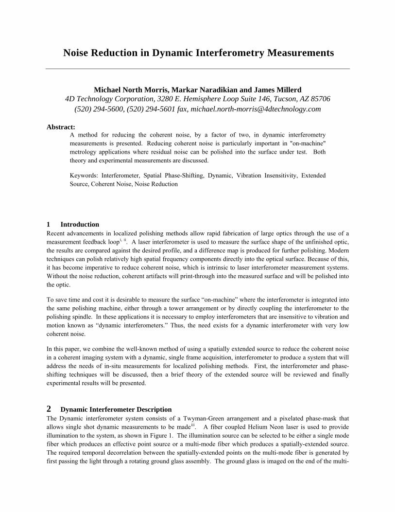
2 Dynamic Interferometer Description The Dynamic interferometer system consists of a Twyman-Green arrangement and a pixelated phase-mask that allows single shot dynamic measurements to be madeiii. A fiber coupled Helium Neon laser is used to provide illumination to the system, as shown in Figure 1. The illumination source can be selected to be either a single mode fiber which produces an effective point source or a multi-mode fiber which produces a spatially-extended source. The required temporal decorrelation between the spatially-extended points on the multi-mode fiber is generated by first passing the light through a rotating ground glass assembly. The ground glass is imaged on the end of the multi-

mode fiber. The light emanating from the multi-mode fiber is psuedo-collimated, and can be considered to be a spectrum of plane waves. The pseudo-collimated beam passes through a linear polarizer to ensure that any effect from birefringence in the fiber is eliminated. An adjustable half-wave plate is used to control the angle of the linearly polarized light which is then split into orthogonally polarized test and reference beams by a polarizing beam splitter. The relative power in the test and reference beams is continuously adjustable by rotating the half-wave plate.

The reference beam passes through a quarter-wave plate oriented to produce circularly polarized light, reflects off the reference mirror and passes through the quarter-wave plate a second time. The linearly polarized light returning from the reference path reflects off the polarizing beam splitter and is directed onto the camera with the pixilated mask via a quarter waveplate that generates the required circularly polarized light. The test arm also has a quarter-wave plate that generates a circularly polarized test beam and rotates the linear polarization leaving the polarizing beam splitter 90 degrees. The difference is that the test beam is polarized horizontally and the reference beam is polarized vertically. As a result, after passing through the quarter-wave plate before the camera the test and reference beams are orthogonally circularly polarized. The orthogonally circularly polarized test and reverence beams impinge on a pixilated phase-mask mounted directly in front of the CCD array. The phase-mask encodes a pixel-wise phase-shift between the test and reference beams facilitating the capture of four phase-shifted interference patterns in a single camera frame capture. The single frame acquisition makes the interferometer substantially immune to vibration and air turbulence.

Camera

PBSQWP

HWP(Adjustable)

Mirror

Interferometer

QWP

HeNe

Test Mirror

Rotating Ground Glass

Multi-Mode Fiber

Pixelated Phase-Mask

Polarizer

Figure 1. Interferometer Schematic: Extended Source Simulated With a Mode Scrambled Multi-Mode Fiber. Single Frame Data Capture Accomplished with Pixelated Phase-Mask.

3 Phase-Shifting Techniques The heart of the measurement system lies in a pixelated phase-mask where each pixel has a unique phase-shift.iv By arranging the phase-steps in a repeating pattern, fabrication of the mask and processing of the data can be simplified.

A small number of discrete steps can be arranged into a “unit cell” which is then repeated contiguously over the entire array. The unit cell can be thought of as a super-pixel; the phase across the unit cell is assumed to change very little. By providing at least three discrete phase-shifts in a unit cell, sufficient interferograms are produced to characterize a sample surface using conventional interferometric algorithms. Figure 1 illustrates a unit cell comprised of four discrete phase steps. Other combinations are possible; however, four phase steps provide optimal sampling. The example shows the phase-steps are in quadrature. For best resolution, a one-to-one correspondence is preferably used between the phase-mask and the detector pixels.

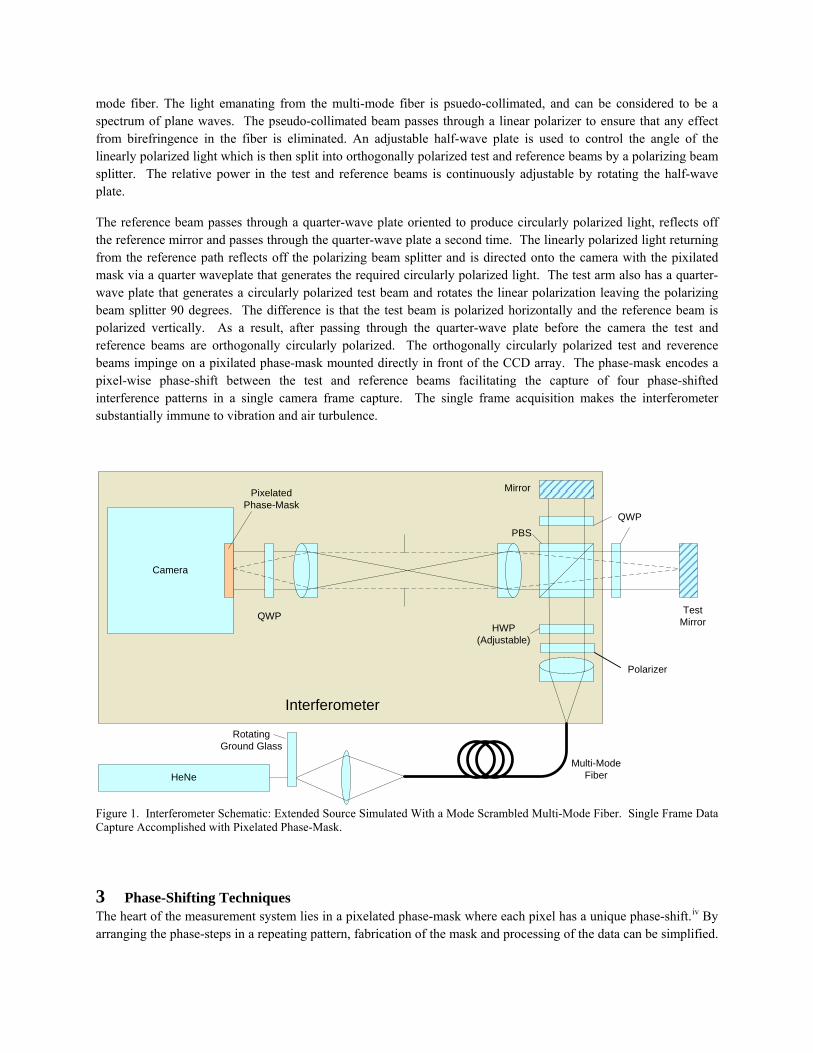
The overall system concept is also shown in Figure 1. and consists of a polarization interferometer that generates a reference wavefront R and a test wavefront T having orthogonal polarization states (which can be linear as well as circular) with respect to each other; a pixelated phase-mask that introduces an effective phase-delay between the reference and test wavefronts at each pixel and subsequently interferes the transmitted light; and a detector array that converts the optical intensity sensed at each pixel to an electrical charge. The pixelated phase-mask and the detector array may be located in substantially the same image plane, or positioned in conjugate image planes.

Figure 2. Basic concept for the pixelated phase-mask dynamic interferometer.

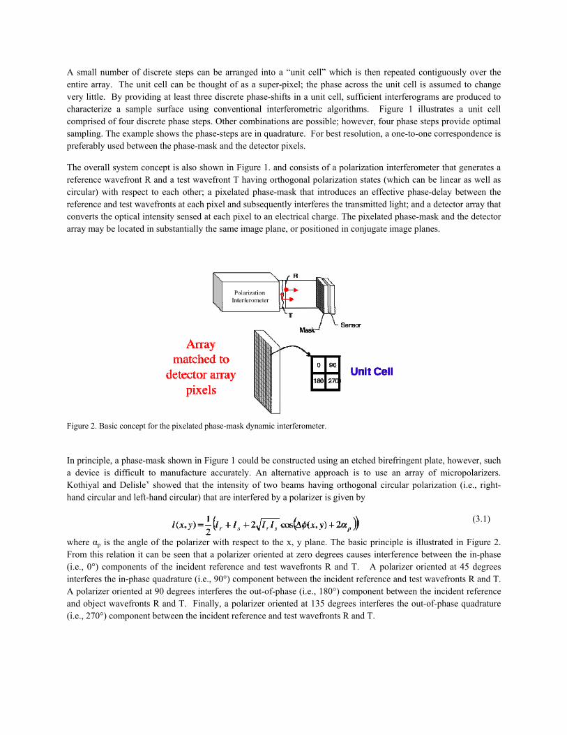
In principle, a phase-mask shown in Figure 1 could be constructed using an etched birefringent plate, however, such a device is difficult to manufacture accurately. An alternative approach is to use an array of micropolarizers. Kothiyal and Delislev showed that the intensity of two beams having orthogonal circular polarization (i.e., right-hand circular and left-hand circular) that are interfered by a polarizer is given by

(3.1)

where αp is the angle of the polarizer with respect to the x, y plane. The basic principle is illustrated in Figure 2. From this relation it can be seen that a polarizer oriented at zero degrees causes interference between the in-phase (i.e., 0°) components of the incident reference and test wavefronts R and T. A polarizer oriented at 45 degrees interferes the in-phase quadrature (i.e., 90°) component between the incident reference and test wavefronts R and T. A polarizer oriented at 90 degrees interferes the out-of-phase (i.e., 180°) component between the incident reference and object wavefronts R and T. Finally, a polarizer oriented at 135 degrees interferes the out-of-phase quadrature (i.e., 270°) component between the incident reference and test wavefronts R and T.

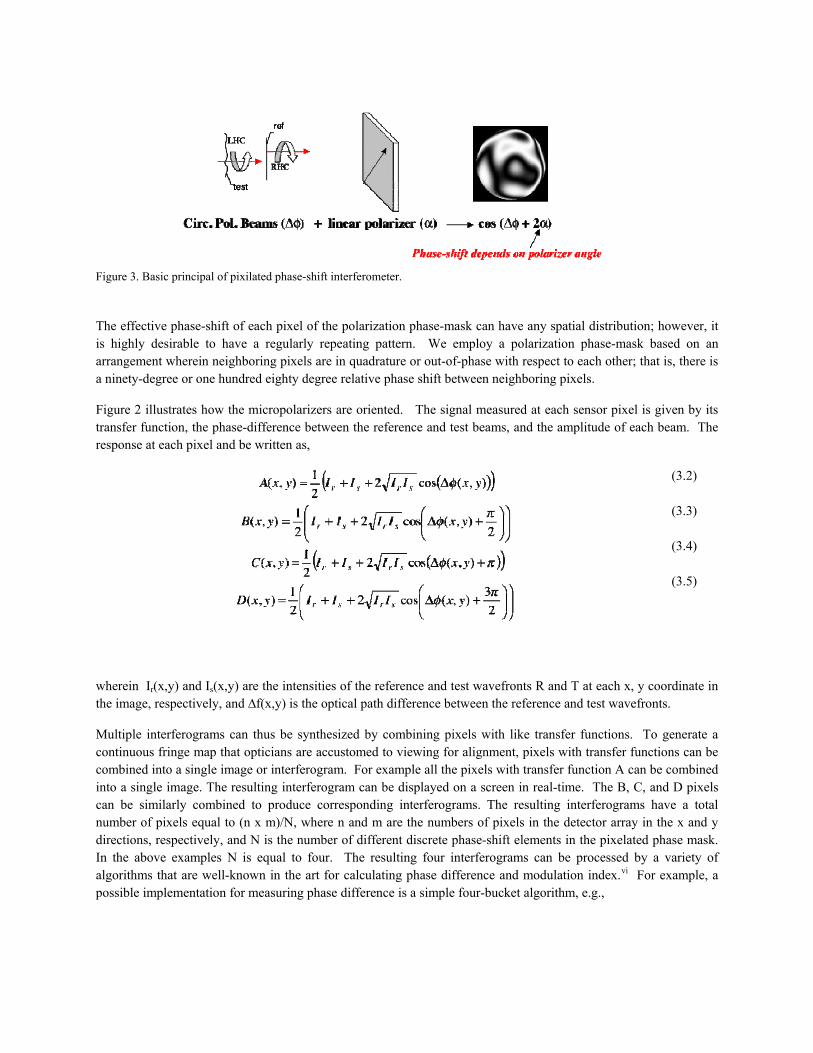
Figure 3. Basic principal of pixilated phase-shift interferometer.

The effective phase-shift of each pixel of the polarization phase-mask can have any spatial distribution; however, it is highly desirable to have a regularly repeating pattern. We employ a polarization phase-mask based on an arrangement wherein neighboring pixels are in quadrature or out-of-phase with respect to each other; that is, there is a ninety-degree or one hundred eighty degree relative phase shift between neighboring pixels.

Figure 2 illustrates how the micropolarizers are oriented. The signal measured at each sensor pixel is given by its transfer function, the phase-difference between the reference and test beams, and the amplitude of each beam. The response at each pixel and be written as,

(3.2) (3.3) (3.4) (3.5)

wherein Ir(x,y) and Is(x,y) are the intensities of the reference and test wavefronts R and T at each x, y coordinate in the image, respectively, and ∆f(x,y) is the optical path difference between the reference and test wavefronts.

Multiple interferograms can thus be synthesized by combining pixels with like transfer functions. To generate a continuous fringe map that opticians are accustomed to viewing for alignment, pixels with transfer functions can be combined into a single image or interferogram. For example all the pixels with transfer function A can be combined into a single image. The resulting interferogram can be displayed on a screen in real-time. The B, C, and D pixels can be similarly combined to produce corresponding interferograms. The resulting interferograms have a total number of pixels equal to (n x m)/N, where n and m are the numbers of pixels in the detector array in the x and y directions, respectively, and N is the number of different discrete phase-shift elements in the pixelated phase mask. In the above examples N is equal to four. The resulting four interferograms can be processed by a variety of algorithms that are well-known in the art for calculating phase difference and modulation index.vi For example, a possible implementation for measuring phase difference is a simple four-bucket algorithm, e.g.,

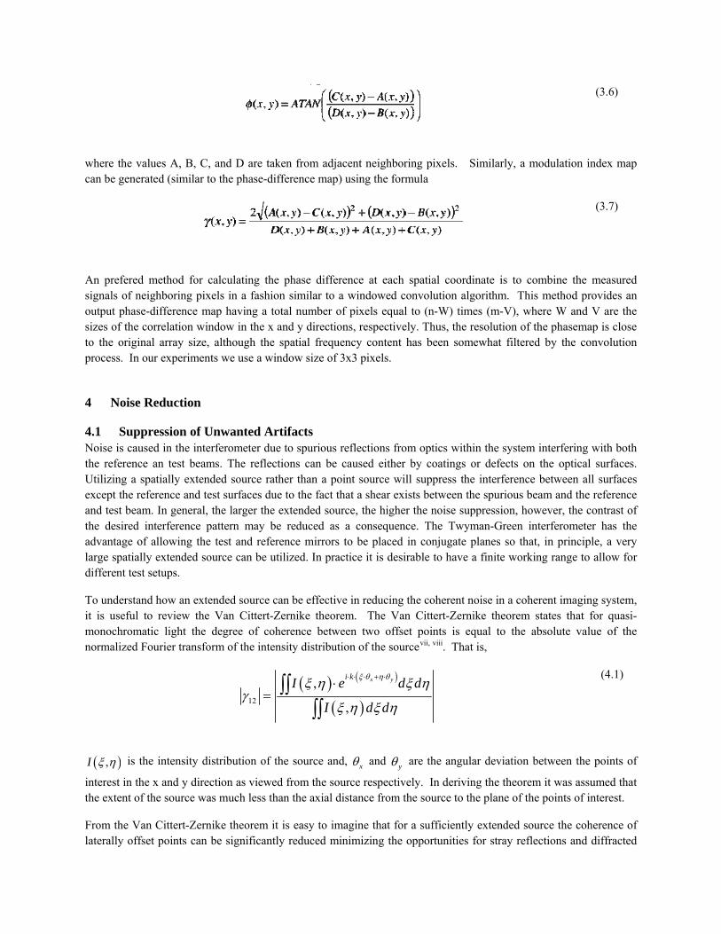
(3.6)

where the values A, B, C, and D are taken from adjacent neighboring pixels. Similarly, a modulation index map can be generated (similar to the phase-difference map) using the formula

(3.7)

An prefered method for calculating the phase difference at each spatial coordinate is to combine the measured signals of neighboring pixels in a fashion similar to a windowed convolution algorithm. This method provides an output phase-difference map having a total number of pixels equal to (n-W) times (m-V), where W and V are the sizes of the correlation window in the x and y directions, respectively. Thus, the resolution of the phasemap is close to the original array size, although the spatial frequency content has been somewhat filtered by the convolution process. In our experiments we use a window size of 3x3 pixels.

4 Noise Reduction

4.1 Suppression of Unwanted Artifacts Noise is caused in the interferometer due to spurious reflections from optics within the system interfering with both the reference an test beams. The reflections can be caused either by coatings or defects on the optical surfaces. Utilizing a spatially extended source rather than a point source will suppress the interference between all surfaces except the reference and test surfaces due to the fact that a shear exists between the spurious beam and the reference and test beam. In general, the larger the extended source, the higher the noise suppression, however, the contrast of the desired interference pattern may be reduced as a consequence. The Twyman-Green interferometer has the advantage of allowing the test and reference mirrors to be placed in conjugate planes so that, in principle, a very large spatially extended source can be utilized. In practice it is desirable to have a finite working range to allow for different test setups.

To understand how an extended source can be effective in reducing the coherent noise in a coherent imaging system, it is useful to review the Van Cittert-Zernike theorem. The Van Cittert-Zernike theorem states that for quasi-monochromatic light the degree of coherence between two offset points is equal to the absolute value of the normalized Fourier transform of the intensity distribution of the sourcevii, viii. That is,

( ) ( )

( )12

,

,

x yi kI e d d

I d d

ξ θ η θξ η ξ ηγ

ξ η ξ η

⋅ ⋅ ⋅ + ⋅⋅= ∫∫

∫∫

(4.1)

( ),I ξ η is the intensity distribution of the source and, xθ and yθ are the angular deviation between the points of

interest in the x and y direction as viewed from the source respectively. In deriving the theorem it was assumed that the extent of the source was much less than the axial distance from the source to the plane of the points of interest.

From the Van Cittert-Zernike theorem it is easy to imagine that for a sufficiently extended source the coherence of laterally offset points can be significantly reduced minimizing the opportunities for stray reflections and diffracted

beam to interfere. The reduction in coherent noise afforded by an extended source has been investigated by many authorsix, x. By taking a slightly more simplified approach the axial coherence of an interferometer cavity for an extended source can be determined.

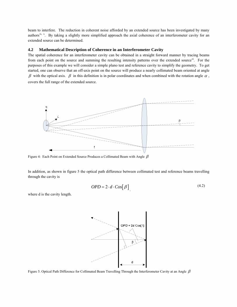
4.2 Mathematical Description of Coherence in an Interferometer Cavity The spatial coherence for an interferometer cavity can be obtained in a straight forward manner by tracing beams from each point on the source and summing the resulting intensity patterns over the extended sourcexi. For the purposes of this example we will consider a simple plano test and reference cavity to simplify the geometry. To get started, one can observe that an off-axis point on the source will produce a nearly collimated beam oriented at angle β with the optical axis. β in this definition is in polar coordinates and when combined with the rotation angle α , covers the full range of the extended source.

Figure 4: Each Point on Extended Source Produces a Collimated Beam with Angle β

In addition, as shown in figure 5 the optical path difference between collimated test and reference beams travelling through the cavity is

[ ]2OPD d Cos β= ⋅ ⋅. (4.2)

where d is the cavity length.

Figure 5. Optical Path Difference for Collimated Beam Travelling Through the Interferometer Cavity at an Angle β

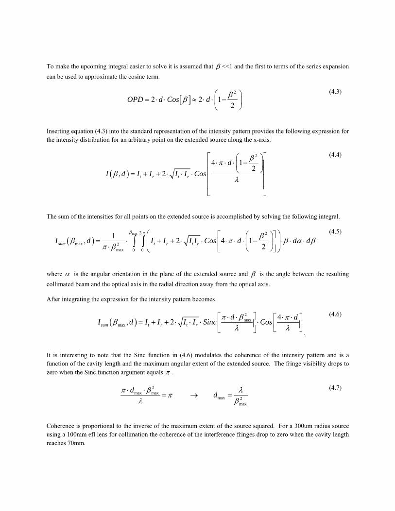
To make the upcoming integral easier to solve it is assumed that β <<1 and the first to terms of the series expansion can be used to approximate the cosine term.

[ ]2

2 2 12

OPD d Cos d ββ⎛ ⎞

= ⋅ ⋅ ≈ ⋅ ⋅ −⎜ ⎟⎝ ⎠

(4.3)

Inserting equation (4.3) into the standard representation of the intensity pattern provides the following expression for the intensity distribution for an arbitrary point on the extended source along the x-axis.

( )

2

4 12

, 2t r t r

dI d I I I I Cos

βπβ

λ

⎡ ⎤⎛ ⎞⋅ ⋅ ⋅ −⎢ ⎥⎜ ⎟

⎝ ⎠⎢ ⎥= + + ⋅ ⋅ ⋅⎢ ⎥⎢ ⎥⎣ ⎦

(4.4)

The sum of the intensities for all points on the extended source is accomplished by solving the following integral.

( )max 2 2

max 2max 0 0

1, 2 4 12sum t r t rI d I I I I Cos d d d

β π ββ π β α βπ β

⋅ ⎛ ⎞⎡ ⎤⎛ ⎞= ⋅ + + ⋅ ⋅ ⋅ ⋅ ⋅ − ⋅ ⋅ ⋅⎜ ⎟⎢ ⎥⎜ ⎟⎜ ⎟⋅ ⎝ ⎠⎣ ⎦⎝ ⎠

∫ ∫ (4.5)

where α is the angular orientation in the plane of the extended source and β is the angle between the resulting collimated beam and the optical axis in the radial direction away from the optical axis.

After integrating the expression for the intensity pattern becomes

( )2max

max4, 2sum t r t r

d dI d I I I I Sinc Cosπ β πβλ λ

⎡ ⎤⋅ ⋅ ⋅ ⋅⎡ ⎤= + + ⋅ ⋅ ⋅ ⋅⎢ ⎥ ⎢ ⎥⎣ ⎦⎣ ⎦ .

(4.6)

It is interesting to note that the Sinc function in (4.6) modulates the coherence of the intensity pattern and is a function of the cavity length and the maximum angular extent of the extended source. The fringe visibility drops to zero when the Sinc function argument equals π .

2

max maxmax 2

max

d dπ β λπλ β

⋅ ⋅= → =

(4.7)

Coherence is proportional to the inverse of the maximum extent of the source squared. For a 300um radius source using a 100mm efl lens for collimation the coherence of the interference fringes drop to zero when the cavity length reaches 70mm.

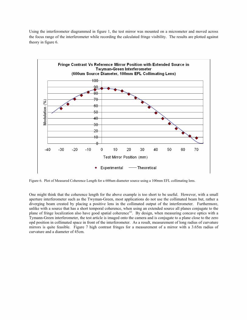
Using the interferometer diagrammed in figure 1, the test mirror was mounted on a micrometer and moved across the focus range of the interferometer while recording the calculated fringe visibility. The results are plotted against theory in figure 6.

Figure 6. Plot of Measured Coherence Length for a 600um diameter source using a 100mm EFL collimating lens.

One might think that the coherence length for the above example is too short to be useful. However, with a small aperture interferometer such as the Twyman-Green, most applications do not use the collimated beam but, rather a diverging beam created by placing a positive lens in the collimated output of the interferometer. Furthermore, unlike with a source that has a short temporal coherence, when using an extended source all planes conjugate to the plane of fringe localization also have good spatial coherencexii. By design, when measuring concave optics with a Tymann-Green interferometer, the test article is imaged onto the camera and is conjugate to a plane close to the zero opd position in collimated space in front of the interferometer. As a result, measurement of long radius of curvature mirrors is quite feasible. Figure 7 high contrast fringes for a measurement of a mirror with a 3.65m radius of curvature and a diameter of 45cm.

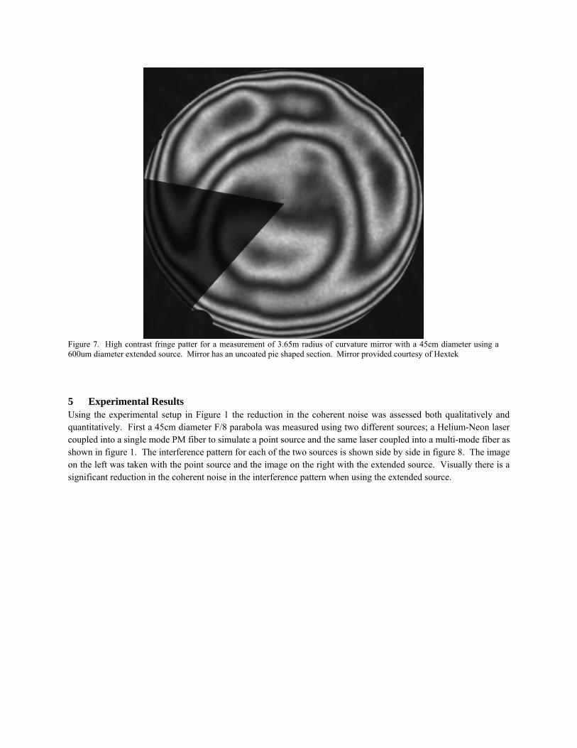
Figure 7. High contrast fringe patter for a measurement of 3.65m radius of curvature mirror with a 45cm diameter using a 600um diameter extended source. Mirror has an uncoated pie shaped section. Mirror provided courtesy of Hextek

5 Experimental Results Using the experimental setup in Figure 1 the reduction in the coherent noise was assessed both qualitatively and quantitatively. First a 45cm diameter F/8 parabola was measured using two different sources; a Helium-Neon laser coupled into a single mode PM fiber to simulate a point source and the same laser coupled into a multi-mode fiber as shown in figure 1. The interference pattern for each of the two sources is shown side by side in figure 8. The image on the left was taken with the point source and the image on the right with the extended source. Visually there is a significant reduction in the coherent noise in the interference pattern when using the extended source.

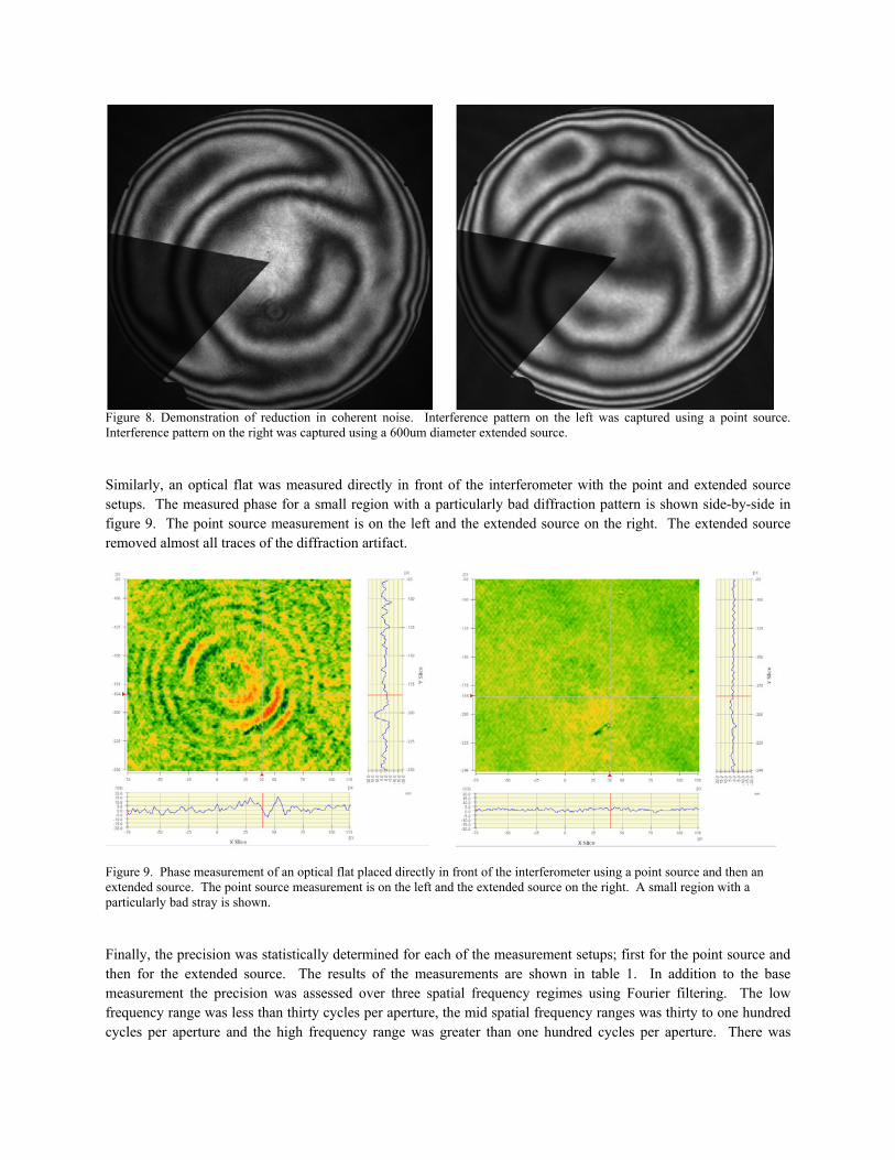
Figure 8. Demonstration of reduction in coherent noise. Interference pattern on the left was captured using a point source. Interference pattern on the right was captured using a 600um diameter extended source.

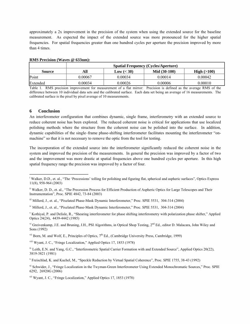
Similarly, an optical flat was measured directly in front of the interferometer with the point and extended source setups. The measured phase for a small region with a particularly bad diffraction pattern is shown side-by-side in figure 9. The point source measurement is on the left and the extended source on the right. The extended source removed almost all traces of the diffraction artifact.

Figure 9. Phase measurement of an optical flat placed directly in front of the interferometer using a point source and then an extended source. The point source measurement is on the left and the extended source on the right. A small region with a particularly bad stray is shown.

Finally, the precision was statistically determined for each of the measurement setups; first for the point source and then for the extended source. The results of the measurements are shown in table 1. In addition to the base measurement the precision was assessed over three spatial frequency regimes using Fourier filtering. The low frequency range was less than thirty cycles per aperture, the mid spatial frequency ranges was thirty to one hundred cycles per aperture and the high frequency range was greater than one hundred cycles per aperture. There was

approximately a 2x improvement in the precision of the system when using the extended source for the baseline measurement. As expected the impact of the extended source was more pronounced for the higher spatial frequencies. For spatial frequencies greater than one hundred cycles per aperture the precision improved by more than 4 times.

RMS Precision (Waves @ 633nm): Spatial Frequency (Cycles/Aperture)

Source All Low (< 30) Mid (30-100) High (>100) Point 0.00067 0.00034 0.00014 0.00042 Extended 0.00034 0.00026 0.00006 0.00010 Table 1. RMS precision improvement for measurement of a flat mirror: Precision is defined as the average RMS of the difference between 10 individual data sets and the calibrated surface. Each data set being an average of 16 measurements. The calibrated surface is the pixel by pixel average of 10 measurements.

6 Conclusion An interferometer configuration that combines dynamic, single frame, interferometry with an extended source to reduce coherent noise has been explored. The reduced coherent noise is critical for applications that use localized polishing methods where the structure from the coherent noise can be polished into the surface. In addition, dynamic capabilities of the single–frame phase-shifting interferometer facilitates mounting the interferometer “on-machine” so that it is not necessary to remove the optic from the tool for testing.

The incorporation of the extended source into the interferometer significantly reduced the coherent noise in the system and improved the precision of the measurements. In general the precision was improved by a factor of two and the improvement was more drastic at spatial frequencies above one hundred cycles per aperture. In this high spatial frequency range the precision was improved by a factor of four.

                                                            i Walker, D.D., et. al., “The ‘Precessions’ tolling for polishing and figuring flat, spherical and aspheric surfaces”, Optics Express 11(8), 958-964 (2003) ii Walker, D. D., et. al., “The Precession Process for Efficient Production of Aspheric Optics for Large Telescopes and Their Instrumentation”, Proc. SPIE 4842, 73-84 (2003) iii Millerd, J., et. al., “Pixelated Phase-Mask Dynamic Interferometer,” Proc. SPIE 5531, 304-314 (2004) iv Millerd, J., et. al., “Pixelated Phase-Mask Dynamic Interferometer,” Proc. SPIE 5531, 304-314 (2004) v Kothiyal, P. and Delisle, R., “Shearing interferometer for phase shifting interferometry with polarization phase shifter,” Applied Optics 24(24), 4439-4442 (1985) vi Greivenkamp, J.E. and Bruning, J.H., PSI Algorithms, in Optical Shop Testing, 2nd Ed., editor D. Malacara, John Wiley and Sons (1992) vii Born, M. and Wolf, E., Principles of Optics, 7th Ed., (Cambridge University Press, Cambridge, 1999) viii Wyant, J. C., “Fringe Localization,” Applied Optics 17, 1853 (1978) ix Leith, E.N. and Yang, G.C., “Interferometric Spatial Carrier Formation with and Extended Source”, Applied Optics 20(22), 3819-3821 (1981) x Freischlad, K. and Kuchel, M., “Speckle Reduction by Virtual Spatial Coherence”, Proc. SPIE 1755, 38-43 (1992) xi Schwider, J., “Fringe Localization in the Twyman-Green Interferometer Using Extended Monochromatic Sources,” Proc. SPIE 6292, 26920G (2006) xii Wyant, J. C., “Fringe Localization,” Applied Optics 17, 1853 (1978)