very long baseline interferometry - yamaguchi...

Tetsuo Sasao and Andre B. FletcherIntroduction to VLBI SystemsChapter 4Lecture Notes for KVN StudentsPartly based on Ajou University Lecture Notes(to be further edited)Version 1. (Unfinished.)Issued on February 19, 2006.

Very Long Baseline Interferometry

Contents

1 Technologies Which Made VLBI Possible 41.1 Basics of Digital Data Processing . . . . . . . . . . . . . . . . 5

1.1.1 Analog Processing Versus Digital Processing . . . . . . 51.1.2 Sampling and Clipping . . . . . . . . . . . . . . . . . . 61.1.3 Discrete–Time Random Process . . . . . . . . . . . . . 61.1.4 Stationary Discrete–Time Random Process . . . . . . . 91.1.5 Sampling . . . . . . . . . . . . . . . . . . . . . . . . . 101.1.6 Comb Function . . . . . . . . . . . . . . . . . . . . . . 121.1.7 Fourier Transform of a Comb Function Is a Comb Func-

tion . . . . . . . . . . . . . . . . . . . . . . . . . . . . 131.1.8 Spectra of Discrete–Time Processes . . . . . . . . . . . 141.1.9 Spectra of Sampled Data . . . . . . . . . . . . . . . . . 171.1.10 Inverse Relations for Spectra of Sampled Data . . . . . 191.1.11 Sampling Theorem . . . . . . . . . . . . . . . . . . . . 201.1.12 Optimum Sampling Interval . . . . . . . . . . . . . . . 221.1.13 Sampling Function . . . . . . . . . . . . . . . . . . . . 251.1.14 Correlations of Nyquist Sampled Data with Rectangu-

lar Passband Spectra . . . . . . . . . . . . . . . . . . . 281.1.15 S/N Ratio of Correlator Output of Sampled Data . . . 331.1.16 Nyquist Theorem and Nyquist Interval . . . . . . . . . 361.1.17 Higher–Order Sampling in VLBI Receiving Systems . . 371.1.18 Clipping (or Quantization) of Analog Data . . . . . . . 391.1.19 Probability Distribution of Clipped Data . . . . . . . . 421.1.20 Cross–Correlation of 1–Bit Quantized Data:

van Vleck Relationship . . . . . . . . . . . . . . . . . . 461.1.21 van Vleck Relationship in Autocorrelation . . . . . . . 51

1

1.1.22 Spectra of Clipped Data . . . . . . . . . . . . . . . . . 511.1.23 Price’s Theorem . . . . . . . . . . . . . . . . . . . . . . 551.1.24 Cross–Correlation of the 2-Bit Quantized Data . . . . . 591.1.25 Cross–Correlation Coefficient of the 2–Bit Quantized

Data . . . . . . . . . . . . . . . . . . . . . . . . . . . . 601.1.26 Power and Cross–Power Spectra of 2-Bit Quantized Data 631.1.27 Dispersion of Digital Correlator Output . . . . . . . . . 661.1.28 S/N Ratio of Digital Correlator Output . . . . . . . . . 671.1.29 Optimum Parameters v0 and n in the 2–Bit Quantization 691.1.30 Effect of Oversampling in S/N Ratio of Clipped Data . 701.1.31 Coherence Factor and Sensitivity with Given Bit Rate 73

1.2 Frequency Standard . . . . . . . . . . . . . . . . . . . . . . . . 761.2.1 VLBI Requires “Absolute” Frequency Stability . . . . . 761.2.2 How to Describe Frequency Stability? . . . . . . . . . . 781.2.3 Types of Phase and Frequency Noises . . . . . . . . . . 801.2.4 Time Domain Measurements . . . . . . . . . . . . . . . 821.2.5 “True Variance” and “Allan Variance” of Fractional

Frequency Deviation . . . . . . . . . . . . . . . . . . . 821.2.6 True Variance and Allan Variance through Power Spec-

trum of Fractional Frequency Deviation . . . . . . . . . 851.2.7 Time–Interval Dependence of Allan Variance . . . . . . 871.2.8 True Variance and Allan Variance through Autocorre-

lation of Phase Noise . . . . . . . . . . . . . . . . . . . 891.2.9 Coherence Function . . . . . . . . . . . . . . . . . . . . 891.2.10 Approximate Estimation of Coherence Time . . . . . . 911.2.11 Estimation of Time–Averaged Phase Noise . . . . . . . 92

1.3 Time Synchronization . . . . . . . . . . . . . . . . . . . . . . 941.4 Recording System . . . . . . . . . . . . . . . . . . . . . . . . . 95

2 Overview of the VLBI System 1012.1 MK–3 As a Prototype of Modern VLBI Systems . . . . . . . . 101

2.1.1 Dual–Frequency Reception . . . . . . . . . . . . . . . . 1022.1.2 First Frequency Conversion . . . . . . . . . . . . . . . 1022.1.3 Transmission to Control Building . . . . . . . . . . . . 1032.1.4 Intermediate Frequency Distributer . . . . . . . . . . . 1032.1.5 Baseband Conversion . . . . . . . . . . . . . . . . . . . 1042.1.6 Formatter . . . . . . . . . . . . . . . . . . . . . . . . . 1062.1.7 Data Recorder . . . . . . . . . . . . . . . . . . . . . . . 1062.1.8 Phase and Delay Calibration . . . . . . . . . . . . . . . 1062.1.9 Hydrogen Maser Frequency Standard . . . . . . . . . . 1082.1.10 Automated Operation by Control Computer . . . . . . 108

2

2.2 Modern VLBI Systems . . . . . . . . . . . . . . . . . . . . . . 1092.2.1 New Recording and Fiber–Link Systems . . . . . . . . 1092.2.2 Digital Baseband Converters . . . . . . . . . . . . . . . 1132.2.3 e–VLBI . . . . . . . . . . . . . . . . . . . . . . . . . . 1142.2.4 VLBI Standard Interface (VSI) . . . . . . . . . . . . . 116

3 Difficulties in Ground–Based VLBI 120

4 Correlation Processing in VLBI 120

5 Observables of VLBI 120

3

1 Technologies Which Made VLBI Possible

Low Noise Amplifier

Video Converter

Formatter

IF Frequency Distributer

Data Recorder

H-Maser Frequency Standard

Correlation Processor

Low Noise Amplifier

Video Converter

Formatter


Data Recorder

Phase and Delay Calibrator


Local Oscillator Local Oscillator

Phase and Delay Calibrator

Digital Data Processing

Figure 1: Schematic view of three major technologies and digital data pro-cessing which realized VLBI.

There were three major technologies which enabled realization of radiointerferometers with very long baselines, exceeding thousands of kilometers.They were:1. high–stability frequency standard,2. high–accuracy time synchronization, and3. high–speed high–density recording, or super–wideband data transmissionin nowadays.

In addition, all signal processings essential to VLBI, such as time marking,recording, delay tracking, fringe stopping, and correlation processing are donedigitally in modern VLBI systems. In this sense, rapid progress in digitaltechnology in the last decades has formed a fundament of VLBI, as illustratedin Figure 1.

4

Therefore, we will first examine theoretical bases of digital signal pro-cessing, to an extent which is necessary to understand principles and rolesof digital circuitries used in VLBI. Then, we will see basic elements of themajor technologies mentioned above.

1.1 Basics of Digital Data Processing

1.1.1 Analog Processing Versus Digital Processing

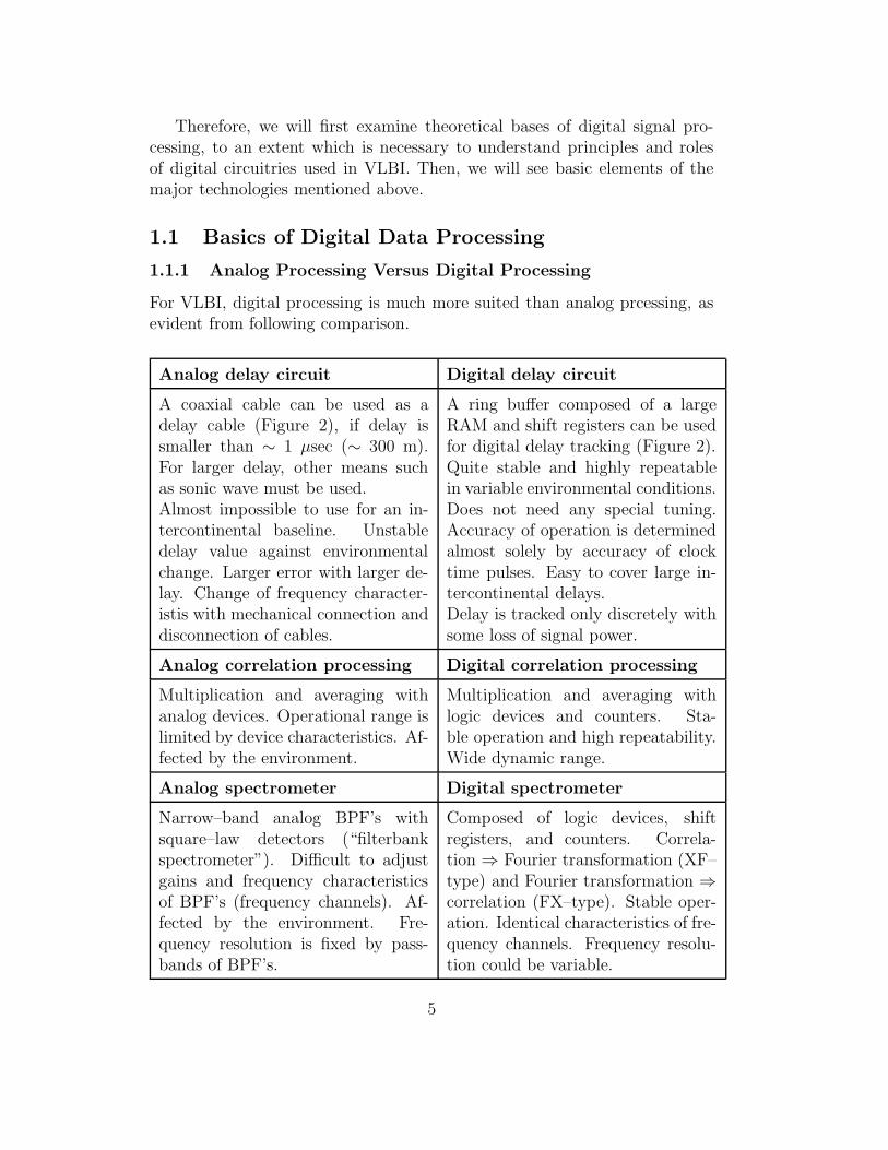
For VLBI, digital processing is much more suited than analog prcessing, asevident from following comparison.

Analog delay circuit Digital delay circuit

A coaxial cable can be used as adelay cable (Figure 2), if delay issmaller than ∼ 1 µsec (∼ 300 m).For larger delay, other means suchas sonic wave must be used.Almost impossible to use for an in-tercontinental baseline. Unstabledelay value against environmentalchange. Larger error with larger de-lay. Change of frequency character-istis with mechanical connection anddisconnection of cables.

A ring buffer composed of a largeRAM and shift registers can be usedfor digital delay tracking (Figure 2).Quite stable and highly repeatablein variable environmental conditions.Does not need any special tuning.Accuracy of operation is determinedalmost solely by accuracy of clocktime pulses. Easy to cover large in-tercontinental delays.Delay is tracked only discretely withsome loss of signal power.

Analog correlation processing Digital correlation processing

Multiplication and averaging withanalog devices. Operational range islimited by device characteristics. Af-fected by the environment.

Multiplication and averaging withlogic devices and counters. Sta-ble operation and high repeatability.Wide dynamic range.

Analog spectrometer Digital spectrometer

Narrow–band analog BPF’s withsquare–law detectors (“filterbankspectrometer”). Difficult to adjustgains and frequency characteristicsof BPF’s (frequency channels). Af-fected by the environment. Fre-quency resolution is fixed by pass-bands of BPF’s.

Composed of logic devices, shiftregisters, and counters. Correla-tion ⇒ Fourier transformation (XF–type) and Fourier transformation ⇒correlation (FX–type). Stable oper-ation. Identical characteristics of fre-quency channels. Frequency resolu-tion could be variable.

5

transmission cable

delay cables

writeaddress

readaddress

delay

input data

delayed output data

ring buffer

Figure 2: Examples of analog delay circuit using delay cables (left) and digitaldelay circuit using a ring buffer (right).

1.1.2 Sampling and Clipping

Two important achievements in the theory of digital data processing werevital for VLBI. They are the sampling theorem by Shannon (1949), and theclipping theorem by van Vleck and Middelton (1966, original work was doneby van Vleck during World War II).

VLBI data are sampled, and clipped (or digitized) with 1–bit or 2–bitquantization (Figure 3).

In the followings, we will see how the information of the analog data isessentially restored from the sampled and clipped data. We will also considersome loss of information accompanied with the digital data processing.

1.1.3 Discrete–Time Random Process

Discrete sequence of variables x[1], x[2], x[3], · · ·, x[i], · · · is called the “ran-dom sequence”, or the “discrete–time random process”, if x[i] at any i is arandom variable, i.e., may vary from trial to trial (Figure 4). This is a “dis-crete version” of the random process continuously varying in time (hence-forth, “continuous–time random process”), which we saw in Chapter 3.

We introduce following statistical concepts for the discrete–time randomprocess.

• Expectation η[i] of a discrete–time random process x[i] (i = 1, 2, 3, · · ·,n, · · ·) is defined by an equation:

η[i] = 〈x[i]〉, (1)

where 〈〉 stands for an ensemble average defined by a joint probabilitydistribution of random variables x[i] (i = 1, 2, 3, · · ·, n, · · ·).

6

0 t

0 t

Sampling

Analog signal

1

-1t

Clipping (or quantization)

0011111110000000000111Bit stream

To digital circuit

Figure 3: Analog–to–digital (A/D) conversion through sampling, clipping,and bit representation. This figure shows a case of 1–bit quantization.

7

trial 1

trial 2

trial 3trial 4trial 5

1 2 3 4 5 6 7 8 9 10 11 i

x[i]

Figure 4: A discrete–time random process is a sequence x[1], x[2], x[3], · · ·,x[i], · · ·, whose value at any i is a random variable.

• Autocorrelation R[m, n] of the discrete–time random process x[i] isdefined by an equation:

R[m, n] = 〈x[m] x∗[n]〉, (2)

where symbol {∗} stands for complex conjugate.

A discrete–time random process x[i] is called the “white noise” if itsautocorrelation satisfies

R[m, n] = 〈| x[m] |2〉 δmn, (3)

where δmn is Kronecker’s delta symbol:

δmn =

1 (m = n)

0 (m 6= n). (4)

• Cross–correlation of two discrete–time random processes:

x[1], x[2], x[3], · · · , x[n], · · ·y[1], y[2], y[3], · · · , y[n], · · ·

is defined byRxy[m, n] = 〈x[m] y∗[n]〉. (5)

8

1.1.4 Stationary Discrete–Time Random Process

The concept of stationary random process, which we introduced in Chapter3 for continuous–time random process, can be transfered to the discrete–timerandom process in the following way (see, for example, Papoulis, 1984).

• Stationary process.A discrete–time random process x[i] is called “stationary” if the expec-tation

η[i] = 〈x[i]〉 = η, (6)

is a constant independent of i, and if the autocorrelation

R[n + m, m] = 〈x[n + m] x∗[n]〉 = R[m], (7)

depends on difference m of arguments only.

In particular, the stationary random discrete–time process is called the“white noise”, if we have

R[m] = R[0] δm0. (8)

• Jointly stationary processes.Two discrete–time random processes x[i] and y[j] are called “jointlystationary” if they are both stationary, and if their cross–correlation

Rxy[n + m, n] = 〈x[n + m] y∗[n]〉 = Rxy[m], (9)


Similarly to the continuous–time process case, we introduce

• correlation coefficient of a zero–mean stationary discrete–time processx[i]:

r[m] =R[m]

R[0], (10)

and

• cross–correlation coefficient of zero–mean jointly stationary discrete–time processes x[i] and y[j]:

rxy[m] =Rxy[m]

√

Rxx[0] Ryy[0], (11)

where, autocovariance is just equal to autocorrelation and cross–covarianceis equal to cross–correlation, since we assumed zero–mean processes (i.e.expectations are equal to zero).

9

1.1.5 Sampling

Let us call the “sampling” an action which makes a discrete–time processby periodically picking up values of a certain continuous–time process with acertain interval of time (“sampling interval”). The discrete–time process thuscreated is called the “time–sample” of the original continuous–time process.

If a discrete–time random process x[n] is a time–sample of a continuous–time random process x(t) with a sampling interval T , i.e. if

x[n] = x(nT ), (12)

then statistical properties of x[n] are determined by statistical properties(i.e., by probability distribution) of x(t).

• Expectation and autocorrelation of a random time–sample.If we denote expectation and autocorrelation of a continuous–time ran-dom process x(t) as η(t) and R(t1, t2), respectively, then expectationand autocorrelation of a random time–sample x[i] = x(iT ) are givenby

η[n] = η(nT ), (13)

andR[m, n] = R(mT, nT ), (14)

respectively.

Proof :

1. η[n] = 〈x[n]〉 = 〈x(nT )〉 = η(nT ).

2. R[m, n] = 〈x[m] x∗[n]〉 = 〈x(mT ) x∗(nT )〉 = R(mT, nT ).

• Cross–correlation of random time–samples.If we denote cross–correlation of continuous–time random processesx(t) and y(t) as Rxy(t1, t2), then cross–correlation of random time–samples x[i] = x(iT ) and y[i] = y(iT ) are given by

Rxy[m, n] = Rxy(mT, nT ). (15)

Proof :

Rxy[m, n] = 〈x[m] y∗[n]〉 = 〈x(mT ) y∗(nT )〉 = Rxy(mT, nT ).

10

• Stationary random time–sample.If a continuous–time random process x(t) is a stationary random pro-cess with constant expectation 〈x(t)〉 = η and autocorrelation〈x(t + τ) x∗(t)〉 = R(τ), then a time–sample x[n] = x(nT ) is a station-ary discrete–time random process with expectation:

η[n] = η, (16)

and autocorrelation:

R[n + m, n] = R[m] = R(mT ). (17)

Proof :

1. Expectation η[n] of the time–sample x[n]

η[n] = 〈x[n]〉 = 〈x(nT )〉 = η,

is a constant independent of argument n.

2. Autocorrelation R[n + m, n] of the time–sample x[n]

R[n + m, n] = 〈x[n + m] x∗[n]〉 = 〈x(mT + nT ) x∗(nT )〉= R(mT ) = R[m],


• Jointly–stationary random time–samples.If x(t) and y(t) are jointly stationary continuous–time random pro-cesses with cross–correlation 〈x(t+τ) y∗(t)〉 = Rxy(τ), then their time–samples x[n] = x(nT ) and y[n] = y(nT ) are jointly stationary discrete–time random processes with cross–correlation:

Rxy[n + m, n] = Rxy[m] = Rxy(mT ). (18)

Proof :

1. Time samples x[n] and y[n] are both stationary discrete–time ran-dom processes, as we saw above.

2. Their cross–correlation

Rxy[n + m, n] = 〈x[n + m] y∗[n]〉 = 〈x(mT + nT ) y∗(nT )〉= Rxy(mT ) = Rxy[m],


11

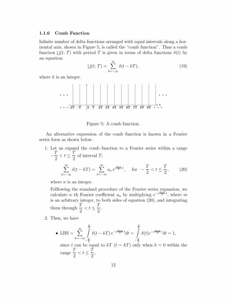
1.1.6 Comb Function

Infinite number of delta functions arranged with equal intervals along a hor-izontal axis, shown in Figure 5, is called the “comb function”. Thus a combfunction

⊔

(t; T ) with period T is given in terms of delta functions δ(t) byan equation:

⊔

(t; T ) =∞∑

k=−∞δ(t − kT ), (19)

where k is an integer.

0 T 2T 3T 4T 5T 6T 7T 8T 9T-T-2Tt. . .

. . .

. . .

. . .

Figure 5: A comb function.

An alternative expression of the comb function is known in a Fourierseries form as shown below.

1. Let us expand the comb function to a Fourier series within a range

−T

2< t ≤ T

2of interval T :

∞∑

k=−∞δ(t − kT ) =

∞∑

n=−∞an ei 2πn

Tt, for − T

2< t ≤ T

2, (20)

where n is an integer.

Folllowing the standard procedure of the Fourier series expansion, wecalculate n–th Fourier coefficient an by multiplying e−i 2πm

Tt, where m

is an arbitrary integer, to both sides of equation (20), and integrating

them throughT

2< t ≤ T

2.

2. Then, we have

• LHS =∞∑

k=−∞

T2∫

−T2

δ(t − kT ) e−i 2πmT

tdt =

T2∫

−T2

δ(t)e−i 2πmT

tdt = 1,

since t can be equal to kT (t = kT ) only when k = 0 within the

rangeT

2< t ≤ T

2,

12

• RHS =∞∑

n=−∞an

T2∫

−T2

ei2π(n−m)

Tt dt = am T,

sinceT2∫

−T2

ei2π(n−m)

Tt dt =

0 if m 6= n

T if m = n.

3. Equating both sides, we have an =1

T, for any n, and hence

∞∑

k=−∞δ(t − kT ) =

1

T

∞∑

n=−∞ei 2πn

Tt, for − T

2< t ≤ T

2. (21)

4. Although we derived this equality in a limited range −T

2< t ≤ T

2, it

actually holds for wider range of t. In fact, functions in the both sidesof equation (21) do not change if we substitute t with t + mT with anarbitrary integer m. This means that they are both periodic functionswith period T . Therefore, equation (21) holds for the whole range of t,i.e. −∞ < t ≤ ∞. Thus, we have a general relation

∞∑

k=−∞δ(t − kT ) =

1

T

∞∑

n=−∞ei 2πn

Tt, (22)

which holds for any t, and, therefore,

⊔

(t; T ) =1

T

∞∑

n=−∞ei 2πn

Tt, (23)

is the alternative expression of the comb function.

1.1.7 Fourier Transform of a Comb Function Is a Comb Function

Fourier transform ˜⊔(ω; T ) of a comb function⊔

(t; T ) of argument t with

period T is a comb function of argument ω with period2π

T(Figure 6).

Proof :According to the general formula of Fourier transformation, we have

˜⊔(ω; T ) =

∞∫

−∞

⊔

(t; T )e−iωt dt =

∞∫

−∞

(

1

T

∞∑

n=−∞ei 2πn

Tt

)

e−iωt dt

13

Comb function with period T

Comb function with period ω0 . . .

. . .0 t

0 ω

Fourier transformation

T

ω0 = 2π Τ

. . .

. . .

Figure 6: Fourier transform of a comb function of t with period T is a comb

function of ω with period ω0 =2π

T.

=1

T

∞∑

n=−∞

∞∫

−∞e−i(ω− 2πn

T ) t dt =2π

T

∞∑

n=−∞δ(

ω − 2πn

T

)

= ω0

∞∑

n=−∞δ(ω − n ω0), (24)

where we introduced a notation:

ω0 =2π

T,

and used the general formula of the delta function:

∞∫

−∞e−iωt dt = 2πδ(ω).

The RHS of equation (24) is nothing but a comb function of ω with a period

ω0 =2π

T:

ω0

∞∑

n=−∞δ(ω − n ω0) = ω0

⊔

(ω; ω0). (25)

Thus,⊔

(t; T ) ⇔ ω0⊔

(ω; ω0),

where a symbol ⇔ implies a Fourier transform pair.

1.1.8 Spectra of Discrete–Time Processes

We introduce following definitions.

14

• Power spectrum.

A power spectrum SD(ω) of a stationary random discrete–time processx[n] with autocorrelation R[m] is given by a discrete Fourier transformwith an arbitrary parameter T (Papoulis, 1984):

SD(ω) =∞∑

m=−∞R[m] e−imωT . (26)

• Cross–power spectrum.

A cross–power spectrum SDxy(ω) of jointly stationary discrete–timeprocesses x[n] and y[n] with cross–correlation Rxy[m] is given by adiscrete Fourier transform with an arbitrary parameter T :

SDxy(ω) =∞∑

m=−∞Rxy[m] e−imωT . (27)

These spectra, as defined by discrete Fourier transforms with an arbitraryparameter T in equations (26) and (27), are periodic functions of ω with

a period2π

T . They have the same forms as Fourier series, with Fourier

coefficients R[m] and Rxy[m], respectively. The spectra SD(ω) and SDxy(ω)are, in general, dependent on the arbitrary parameter T . Later, for particularcases of sampled discrete–time processes (time–samples), we will choose Tto be equal to their sampling intervals. Then, we will be able to establisha relationship between a spectrum of a time–sample and a spectrum of itsoriginal continuous–time process.

• Inverse relations.

Autocorrelation R[m] and cross–correlation RDxy[m] of jointly station-ary random discrete–time processes in equations (26) and (27) are giventhrough the power spectrum SD(ω) and cross–power spectrum SDxy(ω)by inverse relations:

R[m] =T2π

πT∫

− πT

SD(ω) eimωT dω, (28)

Rxy[m] =T2π

πT∫

− πT

SDxy(ω) eimωT dω, (29)

which are nothing but the formulae for Fourier coefficients in the seriesexpansion.

15

Proof :

We prove the inverse relation for the power spectrum SD(ω) given inequation (28) only, since a proof for the cross–power spectrum SDxy(ω)(equation (29)) is given just in a similar way.

1. If SD(ω) =∞∑

n=−∞R[n] e−inωT , then R[m] =

T2π

πT∫

− πT

SD(ω) eimωT dω.

In fact,

T2π

πT∫

− πT

SD(ω) eimωT dω =T2π

∞∑

n=−∞R[n]

πT∫

− πT

ei(m−n)ωT dω = R[m],

sinceπT∫

− πT

ei(m−n)ωT dω =

2πT if n = m,

0 otherwise.

2. If R[m] =T2π

πT∫

− πT

SD(ω) eimωT dω, then SD(ω) =∞∑

n=−∞R[n] e−inωT .

We first prove this statement for a limited range of ω confined

within an interval − π

T < ω ≤ π

T . Inserting first equation to the

RHS of second equation, we have

∞∑

n=−∞R[n] e−inωT =

T2π

πT∫

− πT

SD(ω′)∞∑

n=−∞ein(ω′−ω)T dω′.

Note here that∞∑

n=−∞ein(ω′−ω)T is a comb function given in equation

(23), since, introducing a notation ω0 =2π

T , we have

∞∑

n=−∞ein(ω′−ω)T =

∞∑

n=−∞e

i 2πnω0

(ω′−ω)= ω0

⊔

(ω′ − ω ; ω0)

= ω0

∞∑

k=−∞δ(ω′ − ω − k ω0)

=2π

T∞∑

k=−∞δ(

ω′ − ω − k2π

T)

. (30)

16

Therefore, we obtain

∞∑


∞∑

k=−∞

πT∫

− πT

SD(ω′)δ(

ω′ − ω − k2π

T)

dω′

= SD(ω),

since the delta function in the integrand takes non–zero value when

ω′ = ω + k2π

T ,

and this condition holds only when k = 0, provided that ω is

confined within the interval − π

T < ω ≤ π

T .

Now, if we extend the function SD(ω) to a periodic function with a

period of2π

T , beyond the initially imposed interval − π

T < ω ≤ π

T ,

we have ∞∑

n=−∞R[n] e−inωT = SD(ω),

for any range of ω.

1.1.9 Spectra of Sampled Data

Let us consider discrete–time processes x[n] and y[n], which are time–samplesobtained by sampling jointly stationary continuous–time random processesx(t) and y(t) with a sampling interval T :

x[n] = x(nT ), and y[n] = y(nT ).

Let autocorrelation of x[n], and cross–correlation of x[n] and y[n], be R[m],and Rxy[m], respectively. They satisfy

R[m] = R(mT ), and Rxy[m] = Rxy(mT ),

in view of equations (17) and (18). If we choose the arbitrary parameter Tin the power spectrum SD(ω) and the cross–power spectrum SDxy(ω) of thediscrete–time processes x[n] and y[n], as defined in equations (26) and (27),to be equal to the sampling interval T , i.e.,

T = T, (31)

17

then SD(ω) and SDxy(ω) are related to power spectrum S(ω) and cross–powerspectrum Sxy(ω) of the original continuous–time processes x(t) and y(t) byequations:

SD(ω) =1

T

∞∑

k=−∞S(ω + k ω0), (32)

SDxy(ω) =1

T

∞∑

k=−∞Sxy(ω + k ω0), (33)

where ω0 =2π

T.

Proof :

We prove equation (32) for the power spectrum SD(ω) only, sincea proof of equation (33) for the cross–power spectrum SDxy(ω) isgiven just in a similar way.

According to equations (17), (26), and (31), the power spectrumof the time–sample x[n] = x(nT ) is given by

SD(ω) =∞∑


∞∑

n=−∞R(nT ) e−inωT ,

where T is the sampling interval. Describing the autocorrelationR(τ) of the continuous–time stationary random process x(t) interms of the power spectrum S(ω) through inverse Fourier trans-formation:

R(τ) =1

2π

∞∫

−∞S(ω′) eiω′τ dω′,

we have

SD(ω) =1

2π

∞∑

n=−∞

∞∫

−∞S(ω′) ein(ω′−ω)T dω′

=1

2π

∞∫

−∞S(ω′)

∞∑

n=−∞ein(ω′−ω)T dω′.

According to equation (30),∞∑

n=−∞ein(ω′−ω)T is a comb function:

∞∑

n=−∞ein(ω′−ω)T =

2π

T

∞∑

k=−∞δ(

ω′ − ω − k2π

T

)

.

18

Therefore,

SD(ω) =1

T

∞∑

k=−∞

∞∫

−∞S(ω′) δ(ω′ − ω − k

2π

T) dω′

=1

T

∞∑

k=−∞S(

ω + k2π

T

)

=1

T

∞∑

k=−∞S(ω + k ω0),

where ω0 =2π

T.

1.1.10 Inverse Relations for Spectra of Sampled Data

The inverse relation for the power spectrum SD(ω) of a discrete–time sta-tionary random process x[n]:

R[m] =T

2π

πT∫

− πT

SD(ω) eimωT dω,

as given in equation (28), must yield an autocorrelation which satisfies R[m] =R(mT ), if the process x[n] is a time–sample x[n] = x(nT ) of a continuous–time stationary random process x(t).

Proof :

Substituting equation (32) to the inverse relation, we obtain

R[m] =1

2π

∞∑

k=−∞

πT∫

− πT

S(ω + k2π

T) eimωT dω

=1

2π

∞∑

k=−∞

πT

+k 2πT

∫

− πT

+k 2πT

S(ω′) eim(ω′−k 2πT

)T dω′

=1

2π

∞∑

k=−∞

πT

+k 2πT

∫

− πT

+k 2πT

S(ω′) ei(mω′T−2πkm) dω′

=1

2π

∞∑

k=−∞

πT

+k 2πT

∫

− πT

+k 2πT

S(ω′) eimω′T dω′

=1

2π

∞∫

−∞S(ω′) eimω′T dω′ = R(mT ).

19

Similarly, we confirm that the inverse relation:

Rxy[m] =T

2π

πT∫

− πT

SDxy(ω) eimωT dω,

in equation (29), gives a cross–correlation of time–samples x[n] and y[n]:Rxy[m] = Rxy(mT ).

1.1.11 Sampling Theorem

Shannon (1949) gave a beautiful proof of the sampling theorem, which heformulated as follows:“If a function f(t) contains no frequencies higher than B cps, it is completelydetermined by giving its ordinates at a series of points spaced 1/2B secondsapart.”A mathematical proof showing that “this is not only approximately, butexactly, true” was given as follows.

“Let F (ω) be the spectrum of f(t). Then

f(t) =1

2π

∞∫

−∞F (ω) eiωt dω

=1

2π

2πB∫

−2πB

F (ω) eiωt dω,

since F (ω) is assumed zero outside the band B. If we let

t =n

2B,

where n is any positive or negative integer, we obtain

f(

n

2B

)

=1

2π

2πB∫

−2πB

F (ω) eiω n2B dω.

On the left are the values of f(t) at the sampling points. Theintegral on the right will be recognized as essentially the n–th co-efficient in a Fourier–series expansion of the function F (ω), tak-ing the interval −B to +B as a fundamental period. This meansthat the values of the samples f(n/2B) determine the Fouriercoefficients in the series expansion of F (ω). Thus they determine

20

F (ω), since F (ω) is zero for frequencies greater than B, and forlower frequencies F (ω) is determined if its Fourier coefficients aredetermined. But F (ω) determines the original function f(t) com-pletely, since a function is determined if its spectrum is known.Therefore the original samples determine the function f(t) com-pletely.”

Shannon (1949) mentioned that Nyquist had pointed out the fundamentalimportance of the time interval 1/2B seconds in connection with telegraphy,and proposed to call this the “Nyquist interval” corresponding to the bandB.

Nowadays, we formulate the sampling theorem in a slightly wider form(Figure 7).

t

t

Spectrum of analog continuous-time data

Analog continuous-time signal

Sampled signal

1/(2B)0

0

0 nB (n+1)Bν

-(n+1)B -nB

1/(2B)

Figure 7: Sampling theorem.

Sampling Theorem:All the information in an analog continuous–time signal with a passbandspectrum limited within a frequency range nB ≤ ν < (n + 1)B, where B isa bandwidth and n ≥ 0 is an integer, can be preserved, provided the signal issampled with the Nyquist interval 1/(2B).

Here we assume a real process with even or Hermitian symmetric spec-trum with respect to frequency. Thus, “spectrum” here implies positive fre-quency part of the spectrum. Sampling frequecncy 2B, with Nyquist interval1/(2B), is called the “Nyquist rate”.

21

The proof of the above theorem is given by equations (32) and (33):

SD(ω) =1

T

∞∑

k=−∞S(

ω + k2π

T

)

,

SDxy(ω) =1

T

∞∑

k=−∞Sxy

(

ω + k2π

T

)

,

as illustrated in Figure 8.In fact, equations (32) and (33), and Figure 8, show

• if positive frequency part of the analog continuous–time spectrum S(ω)is confined within a passband nB ≤ ν < (n + 1)B, where n ≥ 0 is aninteger, B is bandwidth, and ν is frequency, and

• if sampling interval T is equal to the Nyquist interval: T = 1/(2B),

then the analog continuous–time spectrum S(ω) is completely preserved inthe spectrum SD(ω) of the sampled data (First and second panels fromthe top of Figure 8). Therefore, all the information of the original ana-log continuous–time signal is preserved in the sampled data. This proves thesampling theorem.

Note, however, that the spectrum SD(ω) of the sampled data in a range0 ≤ ν < B is inverted in frequency compared with the original analogcontinuous–time spectrum S(ω), if the integer n is odd (second panel fromthe top of Figure 8).

On the other hand,

• if the sampling interval T is larger than the Nyquist interval, i.e., T >1/(2B), as shown in the third panel from the top of Figure 8, or, eventhough T = 1/(2B), if the analog continuous–time spectrum is confinedwithin aB ≤ ν < (a + 1)B, where a is not an integer, as shown in thebottom panel of Figure 8,

then foots of spectral components with different n’s in equations (32) and(33) are overlapped with each other (this is called the “aliasing”). There-fore, information of the analog continuous–time spectrum S(ω) is no longerpreserved in the spectrum SD(ω) of the sampled data.

1.1.12 Optimum Sampling Interval

In order to see that the Nyquist interval is the optimum interval for sampling,let us consider an analog continuous–time spectrum which is confined within

22

Spectrum of continuous-time data Spectrum of sampled data

-B0

B

ν

S (ω)

. . .. . .0-1/T 1/T

ν1/2T-1/2T

SD (ω)

0-1/T 1/Tν

1/2T-1/2T

SD (ω)

. . .. . .1/2T-1/2T

S (ω)

-3B -2B -B B 2B 3B0-1/T 1/T1/2T-1/2T

ν-3/2T 3/2T

3/2T

3/2T

-3/2T

-3/2T-3B -2B -B B 2B 3B

B-B1/T-1/T

. . .. . .ν

SD (ω)

0-1/T 1/T1/2T-1/2T

S (ω)

0-1/T 1/T1/2T-1/2Tν

-3/2T 3/2T 3/2T-3/2T-3B -2B -B B 2B 3B -3B -2B -B B 2B 3B

. . .. . .ν

SD (ω)S (ω)

0-1/T 1/T1/2T-1/2Tν

-3/2T 3/2T-3B -2B -B B 2B 3B

0-1/T 1/T1/2T-1/2T 3/2T-3/2T-3B -2B -B B 2B 3B

B

Figure 8: Four cases of relation between spectrum of analog continuous–timedata and spectrum of sampled data given by equations (32) and (33). Top:analog continuous–time spectrum is confined within a passband 2mB ≤| ν |<(2m + 1)B and sampling interval T is equal to Nyquist interval T = 1/(2B).Second from the top: analog continuous–time spectrum is confined withina passband (2m + 1)B ≤| ν |< 2(m + 1)B and T = 1/(2B). Third fromthe top: T > 1/(2B). Bottom: analog continuous–time spectrun is confinedwithin a passband with boundaries of non–integer multiples of B, i.e., aB ≤|ν |< (a+1)B, and T = 1/(2B). Here we adopted notations, ν: frequency, B:bandwidth of the analog continuous–time spectrum, m ≥ 0: an integer, anda: a non–integer number. We assume a real process, and, therefore, an evenor Hermitian symmetric spectrum with respect to frequency. All informationof the original analog continuous–time data is completely preserved in thesampled data in the first two cases, but a part of the information is lost aftersampling in the last two cases.

23

0 Bν

Figure 9: A band–limited baseband spectrum confined within a frequencyrange 0 ≤ ν < B. Here, positive frequency part only is shown.

a baseband 0 ≤ ν < B. Here, the “baseband”, or otherwise called the“video–band”, implies a frequency band containing 0 Hz (or “DC”, whichmeans “direct current”) as the lowest frequency, such as shown in Figure 9.This is a particular case of the passband spectrum within nB ≤ ν < (n+1)Bwhen n = 0. Also, we assume that the bandwidth B here corresponds to anactual extent of the spectrum, that means the spectrum is non–zero in theinside of the interval 0 ≤ ν < B, but zero in the outside.

Then, we can conceive three cases which are shown in Figure 10.

1/2T-1/2T 0 B-B

0 B=1/2T-B=-1/2T

0 B-B1/2T-1/2T

ν

ν

ν

ν

ν

ν

12BT=

12BT<

12BT>

Oversampling

Nyquist sampling

Undersampling

0 1/2T 1/T-1/2T-1/T

0 1/2T 1/T 3/2T 2/T-1/2T-1/T-3/2T-2/T

0 1/T 2/T 3/T-3/T -2/T -1/TB-B

Spectrum of continuous-time data Spectrum of sampled data

Figure 10: Spectra of sampled data in oversampling T < 1/(2B) (top),Nyquist sampling T = 1/(2B) (middle), and undersampling T > 1/(2B)(bottom).

1. OversamplingIf we sample an analog continuous–time signal with sampling interval

24

smaller than the Nyquist interval T < 1/(2B), as shown in top panel ofFigure 10, we will have larger number of data points per unit durationof time, but information contained is not improved at all, comparedwith the Nyquist sampling (sampling with Nyquist interval) case shownin the middle panel of Figure 10. Such a samping with an intervalT < 1/(2B) is called the “oversampling”.

2. UndersamplingOn the contrary, if the sampling interval is larger than the Nyquistinterval T > 1/(2B), a part of information in the original analogcontinuous–time signal is lost in the sampled data due to the alias-ing, as shown in bottom panel of Figure 10. This case is called the“undersampling”.

3. Nyquist samplingTherefore, the Nyquist sampling, i.e. sampling with the Nyquist inter-val T = 1/(2B), is the optimum sampling for an analog continuous–time signal with a band–limited baseband spectrum (middle panel ofFigure 10).

1.1.13 Sampling Function

We saw above that autocorrelation R(τ) and cross–correlation Rxy(τ) ofjointly stationary continuous–time random processes x(t) and y(t) with band–limited baseband spectra are completely restored from autocorrelation R[n] =R(nT ) and cross–correlation Rxy[n] = Rxy(nT ) of time samples of the pro-cesses x[n] = x(nT ) and y[n] = y(nT ), provided that the sampling intervalT is shorter than or equal to the Nyquist interval, i.e. T ≤ 1/(2B), where Bis bandwidth of the spectra. But how can we functionally express R(τ) andRxy(τ) through R[n] and Rxy[n]?

The answer is given by the so–called “second part of the sampling theo-rem”, which states that they satisfy equations:

R(τ) =∞∑

n=−∞R[n]

sin[

πT(τ − nT )

]

πT(τ − nT )

, (34)

and

Rxy(τ) =∞∑

n=−∞Rxy[n]

sin[

πT(τ − nT )

]

πT(τ − nT )

. (35)

The sinc function here:

SAn(τ) ≡sin

[

πT(τ − nT )

]

πT(τ − nT )

, (36)

25

is called the “sampling function”.

Proof :

We prove equation (34) for the autocorrelation only, since equa-tion (35) for the cross–correlation can be derived exactly in thesame way.

According to equation (32), power spectrum S(ω) of a stationaryrandom continuous–time process x(t) and power spectrum SD(ω)of its time–sample x[n] = x(nT ) with a sampling interval T arerelated to each other by

SD(ω) =1

T

∞∑

k=−∞S(

ω + k2π

T

)

.

Therefore, if the sampling interval T is shorter than or equalto the Nyquist interval, T ≤ 1/(2B), we obtain the full analogcontinuous–time baseband spectrum S(ω) by multiplying to thespectrum of the time sample SD(ω) a rectangular window func-tion P (ω) satisfying

P (ω) =

1 − πT

< ω ≤ πT,

0 otherwise,(37)

as illustrated in Figure 11. In fact, we have

S(ω) = T P (ω) SD(ω), (38)

from equation (32).

π/T-π/T 0ω

Continuous-time spectrum S(w) Spectrum of sampled data SD (ω)

ω0 π/T 2π/T-π/T-2π/T

P(ω)

Figure 11: Analog Continuous–Time spectrum S(ω) (left panel) is fully re-stored from spectrum of time samples SD(ω) (right panel) by multiplying arectangular window function P (ω) given in equation (37).

26

If we introduce Fourier transform pairs S(ω) ⇔ R(τ), P (ω) ⇔p(τ) and SD(ω) ⇔ RD(τ), equation (38) implies

R(τ) = T p(τ) ∗ RD(τ) = T

∞∫

−∞p(τ − α) RD(α) dα, (39)

in view of the convolution theorem which we saw in Chapter 3,where symbol “∗” stands for the operation of convolution.

We saw in Chapter 3 that inverse Fourier transform of the rect-angular window function is a sinc function:

p(τ) =1

2π

∞∫

−∞P (ω)eiωτ dω =

1

2π

πT∫

− πT

eiωτ dω =sin

(

πτT

)

πτ. (40)

On the other hand, inverse Fourier transform of equation (32)yields

RD(τ) =1

2π

∞∫

−∞SD(ω)eiωτ dω =

1

2πT

∞∫

−∞

∞∑

k=−∞S(ω + k

2π

T)eiωτ dω

=1

TR(τ)

∞∑

k=−∞e−i 2πk

Tτ = R(τ)

∞∑

n=−∞δ(τ − nT ), (41)

where we used the shift theorem and the property of the combfunction given in equation (22):

1

T

∞∑

k=−∞e−i 2πk

Tτ =

∞∑

n=−∞δ(τ − nT ).

Therefore, equation (39) is reduced to

R(τ) = T∞∑

n=−∞

∞∫

−∞

sin(

πT(τ − α)

)

π(τ − α)R(α) δ(α − nT ) dα

=∞∑

n=−∞R(nT )

sin(

πT(τ − nT )

)

πT(τ − nT )

,

which proves equation (34), since R(nT ) = R[n].

Now we are in position to answer to an interesting question: why ac-curacy of delay determination in VLBI can be much superior (i.e. smaller)

27

than a sampling interval of digitized voltage signals, from which the delay isdetermined? For example, typical delay accuracy of Mark III VLBI systemhas been 0.1 nanosecond (1 × 10−10 sec), while a typical sampling intervalin the Mark III observation has been 125 nanosecond (= 1/(2 × 2 MHz) ).Details apart, an essential point of the answer is in the sampling theorem:Nyquist sampled data are capable of determining the delay as accurately ascontinuous–time data, from which the sampled data are formed, since theyare equivalent to each other in view of the sampling theorem.

The 2B optimal rate and the sampling function have been independentlydiscovered by a number of researchers in different countries, besides Shannon(1949). The history even goes back to the 19th Century. Interested readerscould consult with a review paper by Meijering (2002).

1.1.14 Correlations of Nyquist Sampled Data with RectangularPassband Spectra

Let us consider continuous–time stationary random processes x(t) and y(t)with rectangular power spectra S(ω) with a passband of bandwidth B:

S(ω) =

a 2πnB ≤| ω |< 2π(n + 1)B,

0 otherwise,(42)

where n is an integer, and n = 0 corresponds to the particular case of thebaseband spectrum (Figure 12).

ν = ω /2πnB (n+1)B... ...

-nB-(n+1)B

S(ω)

0 B-B

S(ω)

0 B-B ν = ω /2π

a

a

Figure 12: Rectangular passband (top) and baseband (bottom) power spec-tra.

If we sample the data with Nyquist interval T = 1/(2B), then we obtainfollowing properties for correlations of the time samples.

28

Autocorrelation:Autocorrelation R(τ) of an original continuous–time process x(t) is ob-

tained by an inverse Fourier transformation of the passband power spectrumS(ω) (top panel of Figure 12):

R(τ) =1

2π

∞∫

−∞S(ω) eiωτ dω =

1

π<

∞∫

0

S(ω) eiωτ dω

=a

π<

2π(n+1)B∫

2πnB

eiωτ dω =a

π<

ei2π(n+ 12)Bτ

πB∫

−πB

eiω′τ dω′

=a

π<[

ei2π(n+ 12)Bτ eiπBτ − e−iπBτ

i τ

]

= 2aBsin(πBτ)

πBτcos

[

2π(

n +1

2

)

Bτ]

, (43)

which has the familiar “white–fringe” form with the fringe pattern enclosedby the bandwidth pattern, as we saw in Chapter 3.

In the baseband spectrum (bottom panel of Figure 12), we have n = 0,and the autocorrelation of the continuous–time process has a sinc functionform:

R(τ) = 2aBsin(2πBτ)

2πBτ. (44)

For the correlation coefficient of the continuous–time process:

r(τ) =R(τ)

R(0),

we have,

r(τ) =sin(πBτ)

πBτcos

[

2π(

n +1

2

)

Bτ]

, (45)

in a case of the general passband spectrum, and

r(τ) =sin(2πBτ)

2πBτ, (46)

in the particular case of the baseband spectrum.Now, if we sample the continuous–time process x(t) with the Nyquist

interval T = 1/(2B), correlation coefficient of the time sample is given by

r[m] = r(mT ) =sin

(

mπ2

)

mπ2

cos[

mπ(

n +1

2

) ]

, (47)

29

-1

-0.5

0

0.5

1

-3 -2 -1 0 1 2 3-1

-0.8

-0.6

-0.4

-0.2

0

0.2

0.4

0.6

0.8

1

-3 -2 -1 0 1 2 3

2Bτ

r (τ)

2Bτ

r (τ)

r [m]

m0 1 2 3 4 5-1-2-3-4-5

Figure 13: Correlation coefficient r(τ) of a continuous–time process withrectangular passband spectrum when n = 2 (top left) and baseband spectrum(top right), as given in equations (45) and (46). When this process is sampledwith the Nyquist interval T = 1/(2B), correlation coefficient r[m] of the timesample has the “white–noise” form which is equal to 1 if m = 0, and equalto 0 if m 6= 0 (bottom), since r[m] = r(mT ) = 0 for all m except for m = 0,as shown in the top two panels.

for the passband spectrum, and

r[m] = r(mT ) =sin(mπ)

mπ, (48)

for the baseband spectrum, in particular. Both equations (47) and (48) showthe “white–noise” form of the time sample:

r[m] = δm0 =

1 if m = 0,

0 if m 6= 0,(49)

as given in equation (8), where δij is Kronecker’s delta symbol. This showsthat different sample points are not correlated, and therefore independentof each other, in time samples of Nyquist sampled data with rectangularpassband spectra.

Relationship between the correlation coefficient of the original continuous–time data and that of the sampled data is illustrated in Figure 13.

30

Cross–correlation:If a cross–power spectrum Sxy(ω) of jointly stationary continuous–time

random processes x(t) and y(t) is real (i.e., has zero phase), and rectangu-lar with bandwidth B, such as shown in Figure 12, the situation is muchthe same with the autocorrelation case discussed above, and their cross–correlation has the same functional form as equation (43) or (44). Therefore,cross–correlation coefficient of their time samples has the “white–noise” form,proportional to the one given in equation (49).

Let us now consider a little more general case, when amplitude A(ω) ofthe cross–power spectrum Sxy(ω) is rectangular, as given in equation (42),but phase is non–zero due to some delay τd between correlated signals inprocesses x(t) and y(t), which may in general contain both the signals anduncorrelated noises, just like in an interferometer problem. In such a case,the cross–power spectrum, which contains the signal contribution only, hasa form:

Sxy(ω) = A(ω) e−iωτd, (50)

as we saw in Chapter 3.Strictly speaking, actual passband spectra to be sampled in realistic in-

terferometers are IF spectra after the frequency–conversion, and hence theirphase spectra usually do not cross the origin, i.e., phases are non–zero atω = 0, unlike in equation (50), as we discussed in Chapter 3. Nevertheless,we adopt equation (50) for simplicity, assuming an idealized case of “RFcorrelation”, or a case when the “fringe stopping” is ideally performed sothat the phase crosses the origin, but the phase slope still remains due to animperfect “delay tracking”.

Then, in view of the shift theorem, the cross–correlation Rxy(τ):

Rxy(τ) =1

2π

∞∫

−∞Sxy(ω) eiωτ dω,

should have a similar form as given in equation (43) or (44), but argumentτ is replaced by τ − τd. Thus, cross–correlation coefficient is given by

rxy(τ) =Rxy(τ)

√

Rxx(0) Ryy(0)

=

ρsin[πB (τ − τd)]

πB (τ − τd)cos

[

2π(

n +1

2

)

B (τ − τd)]

(passband),

ρsin[2πB (τ − τd)]

2πB (τ − τd)(baseband),

(51)

31

where ρ is the maximum cross–correlation coefficient:

ρ =Rxy(τd)

√

Rxx(0) Ryy(0). (52)

Note that the cross–correlation coefficient in the case of the passband spec-trum with n 6= 0 again shows the “white–fringe” form with the cosine “fringepattern” enclosed within the sinc function envelope of “bandwidth pattern”.

-1

-0.5

0

0.5

1

-3 -2 -1 0 1 2 3-1

-0.5

0

0.5

1

-3 -2 -1 0 1 2 3

rxy(τ) / ρ rxy[m] / ρrxy[m] / ρ rxy(τ) / ρ

2Bτ2Bτm m

τdτd

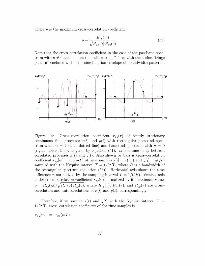
Figure 14: Cross–correlation coefficient rxy(τ) of jointly stationarycontinuous–time processes x(t) and y(t) with rectangular passband spec-trum when n = 2 (left: dotted line) and baseband spectrum with n = 0(right: dotted line), as given by equation (51). τd is a time delay betweencorrelated processes x(t) and y(t). Also shown by bars is cross–correlationcoefficient rxy[m] = rxy(mT ) of time samples x[i] = x(iT ) and y[j] = y(jT )sampled with the Nyquist interval T = 1/(2B), where B is a bandwidth ofthe rectangular spectrum (equation (53)). Horizontal axis shows the timedifference τ normalized by the sampling interval T = 1/(2B). Vertical axisis the cross–correlation coefficient rxy(τ) normalized by its maximum value:

ρ = Rxy(τd)/√

Rxx(0) Ryy(0), where Rxy(τ), Rxx(τ), and Ryy(τ) are cross–

correlation and autocorrelations of x(t) and y(t), correspondingly.

Therefore, if we sample x(t) and y(t) with the Nyquist interval T =1/(2B), cross–correlation coefficient of the time samples is

rxy[m] = rxy(mT )

32

=

ρsin

[

π2

(

m − τd

T

)]

π2

(

m − τd

T

) cos[

π(

n +1

2

) (

m − τd

T

)]

(passband),

ρsin

[

π(

m − τd

T

)]

π(

m − τd

T

) (baseband).

(53)

Relationship between the cross–correlation coefficient of the original continuous–time data and that of the sampled data is illustrated in Figure 14.

The cross–correlation coefficient rxy[m] of the time samples given by equa-tion (53) no longer has the symmetric “white–noise” form, as shown in equa-tion (49) and in the bottom panel of Figure 13, due to the parallel shift of thecross–correlation coefficient of the continuous–time data along the horizontalaxis which is caused by the delay τd. Also, it now depends upon n, i.e. uponlocation of the passband spectrum on the frequency axis, since the “fringepattern” in the “white–fringe” depends on the location.

Thus, in the cross–correlation coefficient, the simple “white–noise” formand the independence of sample points is obtained only when the delay τd isreduced to zero (τd = 0) by a suitable compensating operation, such as the“delay tracking” in the interferometry.

1.1.15 S/N Ratio of Correlator Output of Sampled Data

Let us now imagine a “semi–analog” correlator (non–existing in reality),which would multiply and integrate (i.e. time–average) sampled but notquantized (not clipped) data streams from two antennas of an interferometer.We will estimate here a signal–to–noise ratio of such a correlator, beforeexamining actual digital correlators which deal with sampled and quantizeddata.

Let us assume that the two sampled data streams x[i] and y[i] are timesamples of jointly stationary continuous–time random processes x(t) andy(t), which obey the second–order Gaussian probability distribution, as weassumed in the signal–to–noise–ratio discussion in Chapter 3. We furtherassume that x(t) and y(t) have identical rectangular passband spectra withbandwidth B, as given in equation (42), and they are sampled with theNyquist interval T = 1/(2B). Then, we have x[i] = x(i T ) and y[i] = y(i T ).Also, we assume that the delay tracking and the fringe stopping are perfectelyperformed beforehand, so that the two input data of exactly the same wavefront are being correlated.

In this case, “correlator output” Rs of the sampled data streams is an

33

average of products of time samples over a certain number N :

Rs =1

N

N∑

i=1

x[i] y[i]. (54)

Expectation of this correlator output is nothing but the cross–correlationRxy[0] of x[i] and y[j] at zero argument, since

〈Rs〉 =1

N

N∑

i=1

〈x[i] y[i]〉 =1

N

N∑

i=1

〈x(i T ) y(i T )〉 = Rxy(0) = Rxy[0]. (55)

On the other hand, dispersion of this correlator output σ2s is given by

σ2s = 〈R2

s〉 − 〈Rs〉2, (56)

as we saw in Chapter 3. 〈R2s〉 is described through a double sum of the

fourth statistical momentum in view of equation (54). The fourth statisti-cal momentum is decomposed into a sum of products of second statisticalmomenta (correlations), as we discussed in Chapter 3, since x[i] = x(i T )and y[j] = y(j T ) obey the joint Gaussian probability distribution. Thus, wehave

〈R2s〉 =

1

N2

N∑

i=1

N∑

j=1

〈x[i] y[i] x[j] y[j]〉

=1

N2

N∑

i=1

N∑

j=1

{ 〈x[i] y[i]〉〈x[j] y[j]〉

+ 〈x[i] x[j]〉〈y[i] y[j]〉 + 〈x[i] y[j]〉〈y[i] x[j]〉 }

=1

N2

N∑

i=1

N∑

j=1

{

R2xy[0] + Rxx[i − j] Ryy[i − j] + Rxy[i − j] Rxy[j − i]

}

= 〈Rs〉2 +1

NRxx[0] Ryy[0] +

1

NR2

xy[0]

= 〈Rs〉2 +1

NRxx[0] Ryy[0] (1 + ρ2), (57)

where ρ =Rxy[0]

√

Rxx[0] Ryy[0]=

Rxy(0)√

Rxx(0) Ryy(0)is the maximum cross–correlation

coefficient, given in equation (52), in our assumed case with τd = 0. In de-riving last two lines of equation (57), we used the “white–noise” relations forautocorrelations:

Rxx[i − j] = Rxx[0] δij, and Ryy[i − j] = Ryy[0] δij, (58)

34

in view of equation (49), and for cross–correlation:

Rxy[i − j] = Rxy[0] δij, (59)

which is also satisfied since we assumed τd = 0.Therefore, the dispersion of the correlator output in equation (56) is now

given by

σ2s =

1

NRxx[0] Ryy[0] (1 + ρ2), (60)

and we obtain the signal to noise ratio SNR:

SNR =〈Rs〉σs

=Rxy[0]

√

Rxx[0] Ryy[0] (1 + ρ2)

√N =

ρ√1 + ρ2

√N. (61)

In the expression of the maximum cross–correlation coefficient ρ, the auto-correlations Rxx(0) and Ryy(0) are usually dominated by system noise con-tributions from antenna–receiver systems of a radio interferometer, whilethe cross–correlation Rxy(0) contains contribution of the signal from a ra-dio source only, as we discussed in Chapter 3. Thus, when we observe acontinuum spectrum source, ρ is approximately given by

ρ =

√

TA1 TA2

TS1 TS2

, (62)

as we saw in Chapter 3, where TA1, TA2 are antenna temperatures, whichare assumed constant throughout the frequency band B in the case of thecontinuum spectrum source, and TS1, TS2 are system noise temperatures, ofantenna 1 and antenna 2.

For most of radio sources, TA � TS, and, therefore, ρ � 1. In this case,equation (61) is reduced to

SNR =〈Rs〉σs

= ρ√

N =

√

TA1 TA2

TS1 TS2

√N. (63)

If we denote an integration time of the correlation processing as τa, thenumber of samples N with Nyquist interval 1 / (2 B) is equal to

N = 2 B τa. (64)

Therefore, equation (63) for the continuum spectrum source is reduced to

SNR =

√

TA1 TA2

TS1 TS2

√

2 B τa, (65)

35

which is just identical with what we derived for correlator output of continuous–time voltages in Chapter 3.

This means that the Nyquist sampling does not cause any loss of signal–to–noise ratio of the correlator output, compared with the continuous–timecase, as expected from the sampling theorem. This also means that there isno room for the oversampling, with a sampling rate higher than the Nyquistrate (T < 1 / 2B), in improving the signal–to–noise ratio, despite increasednumber of data points. Thus, the Nyquist sampling is really optimum forthe radio interferometry.

Note that equation (63) can be interpreted as showing√

N–fold improve-ment of the signal–to–noise ratio after repeating and averaging N “measure-ments” of a power (product of two data streams, in our case). This meansthat measurements of a power made at the Nyquist interval are indepen-dent of each other, in the case of the rectangular passband spectra. Thisis a consequence of the independence of time samples themselves discussedearlier.

1.1.16 Nyquist Theorem and Nyquist Interval

The Nyquist theorem (Nyquist, 1928), which we saw in Chapter 2, says thatthermal noise power Wν per unit bandwidth emitted by a resistor in a thermalequilibrium with a temperature T is equal to

Wν = k T, (66)

in the classical limit hν � kT , where k and h are the Boltzmann and rhePlanck constants, respectively. Therefore, energy E emitted within a rect-angular band with a bandwidth B during a time interval t is

E = B t k T. (67)

Since energy per one degree of freedom is equal to1

2k T under the thermal

equilibrium, number of degrees of freedom in this energy must be NF = 2 B t.On the other hand, we have NI = 2 B t Nyquist intervals during the time

t, for the bandwidth B. In the case of the rectangular band, one Nyquistinterval contains one independent sample, as we saw earlier. Therefore, wehave NI independent samples in the emitted energy during the time t.

The equality NI = NF = 2 B t means that one independent sample(Nyquist interval) in the information theory corresponds to one degree offreedom in the physics, in the thermal noise.

36

1.1.17 Higher–Order Sampling in VLBI Receiving Systems

In digital data processings as applied to radio astronomy, sampling of re-ceived voltage signals has been traditionally done at the basebands (or thevideo–bands), containing DC (zero frequency) as the lowest frequency, afterfrequency conversions. This was the safest way for reliable sampling, whenclock rates of sampler circuits were not high enough, and not very stable.

Figure 15: Diagram of receiving system in KVN (Korean VLBI Network)adopting the higher–order sampling technique (figure brought from KVNwebpage http://www.trao.re.kr/ kvn/).

However, it is not easy, in existing analog filtering technology, to im-plement a good enough lowpass filter with sharp rectangular edges. Thissituation has often resulted in rather poor frequency characteristics of thebaseband spectra, and made it difficult to achieve high signal–to–noise ratio,close to the one expected from an ideally rectangular spectrum. Also, be-cause of this difficulty, high quality baseband converters tend to be expensive,especially when wide frequency bands are required.

37

Recently, Noriyuki Kawaguchi and his colleagues successfully applied so–called “higher–order sampling” technique to a number of VLBI systems,including Japanese VERA (VLBI Exploration of Radio Astrometry). Thehigher–order sampling is the sampling at a passband with n > 0, discussedearlier. In general, it is easier to design good analog bandpass filters, withnearly rectangular band shapes, when the ratio B/ν0 of bandwidth B to cen-tral freuency ν0 is smaller. Therefore, it is easier to make a nearly rectangularwideband filter for a passband, than for a baseband. In fact, the higher–ordersampling technique has been effective in wideband receiving systems withtypical bandwidth of 512 MHz or wider, for realizing better frequency char-acteristics and higher signal–to–noise–ratio (Iguchi and Kawaguchi, 2002).

Figure 15 shows a diagram of KVN (Korean VLBI Network) receivingsystem which adopts the higher–order sampling technique. A “basebandconverter” cuts off a 512 MHz band from a 2 GHz–wide first IF signal with8.5 GHz center frequency (i.e. 7.5 – 9.5 GHz band), and converts it to a 512MHz–wide passband signal with 768 MHz central frequency (i.e. 512–1024MHz band), which is then sampled by a high–speed sampler.

Note here that, for the bandwidth B = 512 MHz, the passband nB ≤ ν <(n+1)B with nB = 512 MHz means an odd number of n (i.e. n = 1), whereν is the frequency and n is an integer. Therefore, spectrum of sampled signalis inverted with respect to the spectrum of original continuous–time signal,as we saw in Figure 8. In order to avoid possible inconveniences with theinverted spectra, LO (local oscillator) frequency of the “baseband converter”is chosen so that the passband spectrum is obtained in the lower sideband(LSB), i.e. the spectrum is inverted with respect to the first IF spectrum. Inthis way, one can obtain a spectrum of the sampled signal which is identicalwith the one contained in the first IF signal.

It seems worthwhile to mention an interesting question here. The sam-pling theorem says that the optimal sampling rate for a passband nB ≤ ν <(n + 1)B is 2B. Does this mean that we can use an inexpensive low–speed4 Msps (mega sample per second) sampler for sampling a signal in a high–frequency passband, say, 10.000 – 10.002 GHz? The answer is “NO”, as N.Kawaguchi clearly explains. Although the required sampling interval is really1/(2B), sampling timings must be controlled with much greater accuracy,better than 1/ν0, where ν0 is the central frequency of the passband (the “car-rier” frequency). Otherwise, we will get all chaotically “jittered” data at eachof VLBI stations, from which we will never find any good fringe. Therefore, arequired sampler must be as accurate as, and as stable as, a 20 Gsps sampler,say. Consequently, the high–speed sampling technology is indispensable forsuccessful application of the wideband higher–order sampling technique.

38

1.1.18 Clipping (or Quantization) of Analog Data

The sampling replaces data that are continuous in time with those discretein time. This is undoubtedly a big step towards digitizing analog data.However, the sampling alone still leaves values of time samples analog, whichmay vary arbitrarily from sample to sample. For a complete analog to digital(A/D) conversion, we need to replace each continuously variable value withan element of a finite set of discrete values expressible by a certain numberof bits. This step is called the “clipping” or the “quantization”.

Number of discrete values expressible by a given number of bits deter-mines “number of levels of quantization”. Therefore, 1–bit, 2–bit, · · ·, n–bitquantizations usually correspond to 2–level, 4–level, · · ·, 2n–level quantiza-tions, respectively. There have been exceptions of the n–bit, 2n–level law ofquantization, such as 2–bit, 3–level quantization. However, such exceptionalquantization schemes are rarely used in present–day VLBI systems.

We will denote henceforth a discrete–time process with quantized valuesas x[i]. If number of quantization levels is m, with discrete values x1, x2, · · ·,xm, then x[i] must take one of these m values as illustrated in Figure 16. Aquantized process x[i] is supposed to be related in a prescribed way to anoriginal discrete–time process x[i] with analog values before clipping.

x1

x2

x3

x4

x5

x6

x7

x8

i

x[i]

Figure 16: An image of a quantized discrete–time process.

The larger the number of quantization levels (i.e. bits), the more infor-mation can remain after the clipping. For reducing data size and increasingprocessing speed, however, smaller number of bits is preferable. Thus onehas to choose an optimal number of quantization levels for one’s particu-lar purpose. In VLBI, 1–bit (2–level) and 2–bit (4–level) quantizations aremostly used.

Figure 17 and Table 1 show how quantized values are related to origi-nal analog values in cases of VLBI 1–bit (left panel)and 2–bit (right panel)

39

quantizations.In 1–bit quantization scheme, clipped quantity takes only one of two

values: +1 and −1, depending upon if original analog value is positive ornegative, respectively. It is generally accepted that bit 0 is assigned to −1state and bit 1 is assigned to +1 state.

x

+1

-1

0

0 1bit

x

+n

+1

-1

-n

0-v0 +v0

sign bitmag. bit

0 (1) 0 (1) 1 (0) 1 (0)

0 (1) 1 (0) 0 (0) 1 (1)

x (clipped) x (clipped)

Figure 17: Relations between analog (unquantized) values x and clipped(quantized) values x for 1–bit (left) and 2–bit (right) quantizations, respec-tively. Bit assignments are shown in bottom panels. In case of 2–bit quanti-zation (left), a representative bit assingment for data recorder is shown alongwith that for a correlator chip given in parentheses.

Quantization 1–bit (2–level) 2–bit (4–level)

Analog value x < 0 0 ≤ x x < −v0 −v0 ≤ x < 0 0 ≤ x < v0 v0 ≤ x

Clipped value x = −1 x = +1 x = −n x = −1 x = +1 x = +n

Recorder bit ass. 0 1 s 0, m 0 s 0, m 1 s 1, m 0 s 1, m 1

Correlator bit ass. 0 1 s 1, m 1 s 1, m 0 s 0, m 0 s 0, m 1

Table 1: Clipping criteria and bit assingments of VLBI 1–bit and 2–bit quan-tizations. In the bit assignments for the 2–bit quantization scheme, “s” and“m” stand for sign bit and magnitude bit, respectively.

In 2–bit, 4–level quantization scheme, 4 quantization states are separatedby three threshold values: −v0, 0, and v0. They correspond to 4 clippedvalues: −n, −1, +1, and +n, as shown in left panel of Figure 17 and Table1. Values of parameters v0 and n are chosen so that signal–to–noise ratio

40

of the correlator output is maximized. Note that n thus determined is notnecessarily an integer.

Bit assignments to the 4 quantization states are not uniquely standardizedyet in the 2–bit quantization scheme. Existing VLBI data recording systemsmostly adopt 00, 01, 10, and 11 assignments for −n, −1, +1, and +n states,where first and second bits stand for sign and magnitude bits, respectively,but a widely used 2–bit quantization correlator chip adopts 11, 10, 00, and01 assignments, as shown in Figure 17 and Table 1. Therefore, recorded bitsshould be rearranged before the correlation, when we use a correlator withthe chip.

Sign bits in the 2–bit quantized data are equivalent to 0 and 1 bits inthe 1–bit quantized data. Therefore, it is usually not difficult to cross–correlate 1–bit quantized and 2–bit quantized data, which are obtained indifferent stations in the same VLBI observation with the same samplingrate, using a 1–bit correlation mode, if we sacrify some of information in the2–bit quantized data. In this case, the only necessary thing is to pick up signbits from the 2–bit qunatized data and cross–correlate them with the 1–bitquantized data. Of course, direct cross–correlation of data with differentquantization schemes, such as 1–bit and 2–bit, can be performed withoutloosing information (see, for example, Hagen and Farley, 1973), providedthat a special logical circuit for this purpose is built in a correlator.

0 t

Analog signal

+v0

-v0

2-bit quantized signal

+1

-1t

+n

-n

Figure 18: A schematic view of time variation of original analog data (top)and 2–bit quantized data (bottom).

In the 1–bit quantization scheme, only sign information of the originalanalog data remains in the clipped data, and no information on magnitude(amplitude) is left at all, as illustrated in Figure 3. In the 2–bit quantized

41

data, some information on the magnitude (amplitude) of the analog data isleft, as illustrated in Figure 18, but the information is very vague.

Then, how much can we restore scientific information contained in theoriginal analog data of VLBI after clipping them with 1–bit or 2–bit quanti-zation scheme, which looks quite rough at least at the first glance?

The clipping theorem gives a surprising answer. The theorem was orig-inally developed by J.H. van Vleck in a study of radar–jamming during theWorld War II conducted by the Radio Research Laboratory of Harvard Uni-versity (Report No.51 on July 21, 1943), and was made public more than 20years later by van Vleck and Middleton (1966).

1.1.19 Probability Distribution of Clipped Data

Before proceeding to the clipping theorem, we will examine how we candescribe probability distribution of clipped data.

As we discussed earlier, signals from astronomical radio sources, as well assystem noises produced in antenna–receiving systems and in environments,are well approximated by Gaussian random processes. Therefore, let us con-sider the data as jointly stationary continuous–time random processes x(t)and y(t), which obey the second–order Gaussian probability density, intro-duced in Chapter 3. Here we assume a zero–mean case (i.e. expectationsof x(t) and y(t) are equal to zero), and use notations suited to the currentdiscussions, slightly changing those adopted in Chapter 3. Also, we assumethat both x(t) and y(t) are real processes.

Then, we describe the zero–mean second–order Gaussian probability den-sity of jointly stationary continuous–time random processes x(t+ τ) and y(t)as:

f(x, y; τ) ≡ f(x, y; t + τ, t)

=1

2πσxσy

√

1 − r2xy(τ)

e− 1

2[1 − r2xy(τ)]

[

x2

σ2x

− 2 rxy(τ)x y

σx σy

+y2

σ2y

]

, (68)

where we introduced notations: σ2x ≡ Rxx(0), σ2

y ≡ Ryy(0), for dispersions ofx(t) and y(t), and

rxy(τ) ≡ Rxy(τ)√

Rxx(0) Ryy(0),

for cross–correlation coefficient of x(t+τ) and y(t). Here, Rxy(τ), Rxx(τ), andRyy(τ) are cross–correlation and autocorrelations of x(t) and y(t), as before.We first assume that the cross–correlation coefficient rxy(τ) is smaller than

42

1 in absolute value (i.e. r2xy(τ) < 1) in order to avoid possible singularity in

our calculations which may ocur when r2xy(τ) = 1.

x(t)

y(t)

x+dxx

y+dyy

t

t+τ time

time

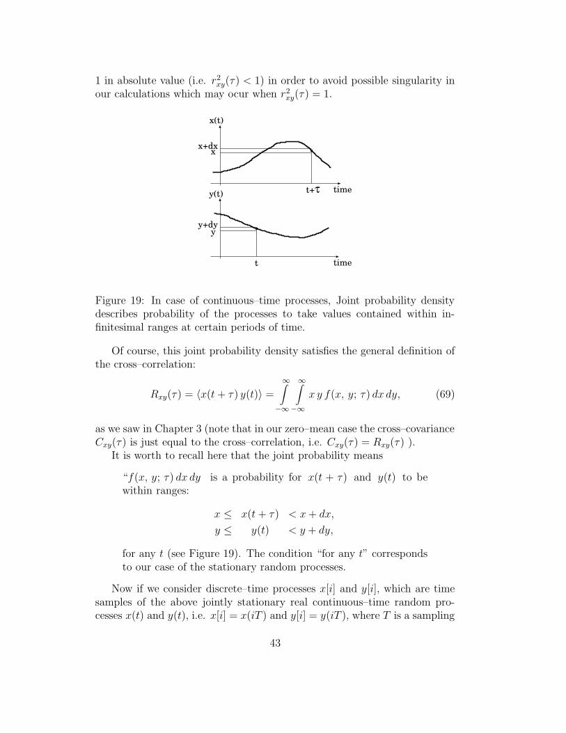
Figure 19: In case of continuous–time processes, Joint probability densitydescribes probability of the processes to take values contained within in-finitesimal ranges at certain periods of time.

Of course, this joint probability density satisfies the general definition ofthe cross–correlation:

Rxy(τ) = 〈x(t + τ) y(t)〉 =

∞∫

−∞

∞∫

−∞x y f(x, y; τ) dx dy, (69)

as we saw in Chapter 3 (note that in our zero–mean case the cross–covarianceCxy(τ) is just equal to the cross–correlation, i.e. Cxy(τ) = Rxy(τ) ).

It is worth to recall here that the joint probability means

“f(x, y; τ) dx dy is a probability for x(t + τ) and y(t) to bewithin ranges:

x ≤ x(t + τ) < x + dx,

y ≤ y(t) < y + dy,

for any t (see Figure 19). The condition “for any t” correspondsto our case of the stationary random processes.

Now if we consider discrete–time processes x[i] and y[i], which are timesamples of the above jointly stationary real continuous–time random pro-cesses x(t) and y(t), i.e. x[i] = x(iT ) and y[i] = y(iT ), where T is a sampling

43

interval, the time samples x[i] and y[i] are also jointly stationary as we sawearlier, and their cross–correlation:

Rxy[m] = 〈x[n + m] y[n]〉 = Rxy(mT ) = 〈x(nT + mT ) y(nT )〉is described by the same joint probability density of the continuous–timeprocesses f(x, y; τ) as

Rxy[m] = Rxy(mT ) =

∞∫

−∞

∞∫

−∞x y f(x, y; mT ) dx dy. (70)

Let us then consider that we clip the time samples x[i] and y[i], andobtain clipped discrete–time processes which we denote as x[i] and y[i]. Theynow take only discrete values of a finite number N (this means N–levelquantization) x1, x2, · · ·, xN and y1, y2, · · ·, yN .

x[i]

y[i]^

^

i

in

n+m

x1

x5

x4

x3

x2

y1

y5

y4

y3

y2

Figure 20: Joint probability P (xi, yj; m) of clipped processes x[n + m] andy[n] describes probability for them to take certain discrete values xi and yj

on quantization levels (here 5–level case is shown).

In this case, their cross–correlation Rxy[m] = 〈x[n + m] y[n]〉 is decribedby an equation:

Rxy[m] =N∑

i=1

N∑

j=1

xi yjP (xi, yj; m), (71)

where P (xi, yj; m) is a joint probability for x[n+m] and y[n] to take values:

x[n + m] = xi,

y[n] = yj,

44

for any n (See Figure 20).This cross–correlation is what should be yielded by a digital correlator.

In fact, in view of the ergodicity, the cross–correlation is well approximatedby a time–average of products of N quantized data x[n + m] and y[n]:

Rxy[m] ∼= 1

NN∑

n=1

(x[m + n] y[n]), (72)

if N is sufficiently large; and the digital correlator is nothing but a machinewhich time–averages a large number of products of digital (i.e. sampled andclipped) data.

At the first glance, equations (70) and (71) look quite different, and itappears difficult to relate Rxy[m] with Rxy[m]. However, if the quantizationcondition is clearly specified, we can calculate P (xi, yj; m) rather easily fromf(x, y; mT ) (van Vleck and Middleton, 1966).

In case of the 1–bit, 2–level quantization, the condition is

x[i] =

+1 for x[i] = x(iT ) ≥ 0,

−1 for x[i] = x(iT ) < 0,

y[i] =

+1 for y[i] = y(iT ) ≥ 0,

−1 for y[i] = y(iT ) < 0.(73)

Therefore, the probability for x[i] to be +1, for example, is nothing but theprobability for x(iT ) to be 0 ≤ x(iT ) < +∞. Thus we can describe jointprobabilities for all combinations of quantization states through equations:

P (+1, +1; m) =

+∞∫

0

+∞∫

0

f(x, y; mT ) dx

dy,

P (−1, −1; m) =

0∫

−∞

0∫

−∞f(x, y; mT ) dx

dy,

P (+1, −1; m) =

0∫

−∞

+∞∫

0

f(x, y; mT ) dx

dy,

P (−1, +1; m) =

+∞∫

0

0∫

−∞f(x, y; mT ) dx

dy. (74)

Integrals in the RHS of these equations are readily calculated, since f(x, y; mT )is given by the joint Gaussian probability density in equation (68).

45

1.1.20 Cross–Correlation of 1–Bit Quantized Data:van Vleck Relationship

In case of the 1–bit quantization, we have

N = 2, and

x1 = −1, x2 = +1,

y1 = −1, y2 = +1.(75)

Therefore, cross–correlation Rxy of clipped data x[i] and y[i] is given by

Rxy[m] =2∑

i=1

2∑

j=1

xi yj P (xi, yj; m)

= (+1) · (+1) · P (+1, +1; m) + (−1) · (−1) · P (−1, −1; m)

+ (+1) · (−1) · P (+1, −1; m) + (−1) · (+1) · P (−1, +1; m)

= P (+1, +1; m) + P (−1, −1; m)

− P (+1, −1; m) − P (−1, +1; m). (76)

Because of symmetric properties of the joint Gaussian probability densityshown in equation (68), the joint probabilities given in equation (74) satisfy

P (+1, +1; m) = P (−1, −1; m),

P (+1, −1; m) = P (−1, +1; m). (77)

Also, by definition of the probability, sum of probabilities of all possible casesmust be equal to 1, and hence

P (+1, +1; m) + P (−1, −1; m) + P (+1, −1; m) + P (−1, +1; m)

= 2 P (+1, +1; m) + 2 P (+1, −1; m) = 1. (78)

Then, from equations (76), (77), and (78), we obtain

Rxy[m] = P (+1, +1; m) + P (−1, −1; m)

− P (+1, −1; m) − P (−1, +1; m)

= 2 P (+1, +1; m) − 2 P (+1, −1; m)

= 4 P (+1, +1; m) − 1. (79)

Substituting the explicit form of the joint Gaussian probability densityin equation (68) into equation (74), we calculte 4 P (+1, +1; m):

4 P (+1, +1; m) = 4

+∞∫

0

+∞∫

0

f(x, y; mT ) dx

dy

46

=

+∞∫

0

+∞∫

0

2

πσxσy

√

1 − r2xy

e− 1

2(1 − r2xy)

(

x2

σ2x

− 2 rxyx y

σx σy+

y2

σ2y

)

dx

dy,

(80)

where T is the sampling interval, as before, and we denoted the cross–correlation coefficient rxy[m] = rxy(mT ) as rxy, for simplicity.

Let us introduce new variables ζ and φ, which satisfy

x = σx ζ cos φ,

y = σy ζ sin φ. (81)

Then the above integral is reduced to

4 P (+1, +1; m) =2

π√

1 − r2xy

π2∫

0

dφ

∞∫

0

e−ζ2(1 − rxy sin 2φ)

2(1 − r2xy) ζ dζ

=2

π

π2∫

0

√

1 − r2xy

1 − rxy sin 2φdφ . (82)

If we further introduce another new variable θ, which satisfies

tan θ =tanφ − rxy√

1 − r2xy

, and, therefore, θ = arctan

tanφ − rxy√

1 − r2xy

, (83)

then we have

dθ

dφ=

1

1 +(

tan φ−rxy√1−r2

xy

)2

1√

1 − r2xy

1

cos2 φ=

√

1 − r2xy

1 − rxy sin 2φ. (84)

Note that this has the same form as the integrand of equation (82). The

limits of the integration φ = 0 and φ =π

2now correspond to

θ = θ0 ≡ − arctan

rxy√

1 − r2xy

and θ =π

2, respectively. Terefore, equation

(82) becomes

4 P (+1, +1; m) =2

π

π2∫

θ0

dθ = 1 − 2

πθ0 = 1 +

2

πarctan

rxy√

1 − r2xy

. (85)

47

Denoting the cross–correlation coefficient rxy through a sine function:

rxy = sin ξ, and, therefore,rxy

√

1 − r2xy

= tan ξ,

we obtain

4 P (+1, +1; m) = 1 +2

πarctan(tan ξ) = 1 +

2

πξ = 1 +

2

πarcsin(rxy). (86)

We must specify here a range of arcsin(rxy), since, in general, arcsine isa multi–value function, while the probability P (+1, +1; m) is certainly not.In view of the general property of the probability, P (+1, +1, m) must beconfined within a range:

0 ≤ P (+1, +1, m) ≤ 1

2.

Indeed, the upper limit corresponds to a case of the complete correlation(identical data), for which

P (+1, +1; m) = P (−1, −1; m) =1

2,

becauseP (+1, −1; m) = P (−1, +1; m) = 0,

while the lower limit corresponds to a case of the complete anti–correlation(identical data but with different signs), for which

P (+1, +1; m) = P (−1, −1; m) = 0.

Since the cross–correlation coefficient rxy of the original unclipped data mustbe 1 in the complete correlation, and −1 in the complete anti–correlation,the arcsine function in equation (86) must be confined within a range:

−π

2≤ arcsin(rxy) ≤

π

2. (87)

Finally, from equation (79), we obtain

Rxy[m] = 4P (+1, +1; m) − 1 =2

πarcsin(rxy[m])

=2

πarcsin

Rxy(mT )√

Rxx(0) Ryy(0)

. (88)

48

Since x[i] x[i] = 1 and y[i] y[i] = 1 for any i, and therefore Rxx[0] = 1 andRyy[0] = 1, for the 1–bit quantized data, their cross–correlation coefficient isequal to their cross–correlation:

rxy[m] =Rxy[m]

√

Rxx[0] Ryy[0]= Rxy[m]. (89)

Therefore, equation (88) is described also as

rxy[m] =2

πarcsin(rxy[m]). (90)

In a particular case of a small cross–correlation coefficient | rxy[m] |� 1,which is usually the case in radio interferometry, we have an approximatelinear equation:

rxy[m] =2

πrxy[m]. (91)

Although we derived equations (88) and (90) assuming that r2xy < 1, it is

worth to confirm here that the resultant equations are valid in the limitingcases of the complete correlation (rxy = 1 and rxy = 1) and the completeanti–correlation (rxy = −1 and rxy = −1), too.

Equation (88) or (90) is generally called the “van Vleck relationship”.This is indeed a surprising result which shows that the cross–correlationcoefficient rxy[m] of the original analog data is almost completely restoredfrom the cross–correlation coefficient rxy[m] of the 1–bit quantized data bya simple equation:

rxy[m] = sin(

π

2rxy[m]

)

. (92)

In the case of the small cross–correlation coefficient | rxy[m] |� 1, we have

rxy[m] =π

2rxy[m]. (93)

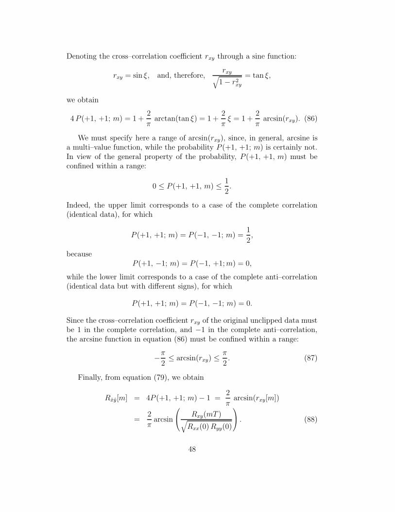
As we saw before, cross–correlation Rxy[m] (= rxy[m]) of digital data isreadily obtained from a digital correlator. Therefore, equations (92) and (93)mean that, we can completely derive functional form and, therefore,spectral shape of the original cross–correlation coefficient from anoutput Rxy[m] of a digital correlator of the 1–bit quantized data, though theamplitude is reduced by a factor of ∼= 2/π (see, for example, Fifure 21).

It is natural that the cross–correlation Rxy(mT ) itself of the original ana-log data cannot be directly obtained from the 1–bit quantized data alonewhich carries sign information only. Nevertheless, we can restore the cross–correlation Rxy(mT ) of the original analog data, if their dispersions Rxx(0)

49

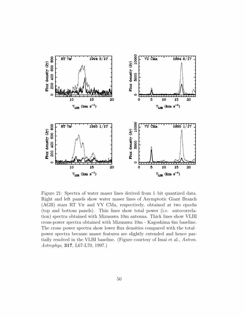
Figure 21: Spectra of water maser lines derived from 1–bit quantized data.Right and left panels show water maser lines of Asymptotic Giant Branch(AGB) stars RT Vir and VY CMa, respectively, obtained at two epochs(top and bottom panels). Thin lines show total–power (i.e. autocorrela-tion) spectra obtained with Mizusawa 10m antenna. Thick lines show VLBIcross-power spectra obtained with Mizusawa 10m - Kagoshima 6m baseline.The cross–power spectra show lower flux densities compared with the total–power spectra because maser features are slightly extended and hence par-tially resolved in the VLBI baseline. (Figure courtesy of Imai et al., Astron.Astrophys, 317, L67-L70, 1997.)

50

and Ryy(0) are known, for example, from suitable system–noise measure-ments.

Derivation of this relationship owes to the clever use of the probabil-ity relations in equation (74) by van Vleck. Note that J.H. van Vleck is ascientist who in 1977 received Nobel Prize in Physics in his major field ofresearch: the “fundamental theoretical investigations of the electronic struc-ture of magnetic and distorted systems”.

1.1.21 van Vleck Relationship in Autocorrelation

Although we examined the derivation of the van Vleck relationship for cross–correlation, there is no restriction in applying the same logic to autocorre-lation of a zero–mean stationary random process x(t). As a matter of fact,van Vleck originally derived his relationship for the autocorrelation. Theonly difference is that we have to use, instead of equation (68), second–orderGaussian probability density for values of x(t) taken at times t + τ and t:

f(x1, x2; τ) =1

2πσ2x

√

1 − r2xx(τ)

e− 1

2(1 − r2xx(τ))

(

x21 − 2rxx(τ) x1x2 + x2

2

σ2x

)

,

(94)

where σ2x = Rxx(0) is the dispersion and rxx(τ) =

Rxx(τ)

Rxx(0)is the correlation

coefficient of x(t).Exactly the same logic as in the cross–correlation case leads to an equa-

tion:

rxx[m] = Rxx[m] =2

πarcsin(rxx[m]) =

2

πarcsin

(

Rxx(mT )

Rxx(0)

)

, (95)

for the correlation coefficient of the 1–bit quantized data x[i], which is thevan Vleck relationship in the autocorrelation.

1.1.22 Spectra of Clipped Data

The derivation of the van Vleck relationship, as we saw above, is quite generaland applicable to any data obeying joint Gaussian probability density. Inparticular, the relationship is well valid for continuous–time data, though wehave dealt with only sampled data in our discussion of digitization of analogdata. Thus, we generally have

Rxy(τ) =2

πarcsin(rxy(τ)), (96)

51

for the cross–correlation, and

Rxx(τ) =2

πarcsin(rxx(τ)), and Ryy(τ) =

2

πarcsin(ryy(τ)), (97)

for the autocorrelations, with arbitrary time interval τ .Therefore, we can calculate cross–power spectrum Sxy(ω), and power

spectra Sxx(ω) and Syy(ω) of clipped data in terms of the ordinary Fouriertransformations:

Sxy(ω) =

∞∫

−∞Rxy(τ) e−iωτ dτ =

2

π

∞∫

−∞arcsin(rxy(τ)) e−iωτ dτ,

Sxx(ω) =

∞∫

−∞Rxx(τ) e−iωτ dτ =

2

π

∞∫

−∞arcsin(rxx(τ)) e−iωτ dτ,

Syy(ω) =

∞∫

−∞Ryy(τ) e−iωτ dτ =

2

π

∞∫

−∞arcsin(ryy(τ)) e−iωτ dτ. (98)

Let us consider a case when analog data have rectangular spectra. This isan important case from a practical point of view, since rectangular bandpassfilters are widely adopted in radio astronomy. We saw earlier that correlationcoefficients of analog data take sinc function forms when their spectra arerectangular. Then, how spectra of the data will look like after clipping?

Figure 22 shows a power spectrum Sxx(ω) of 1–bit quantized data (solidline in bottom panel) which is derived from analog data with a rectangularpower spectrum Sxx(ω) of bandwidth B (broken line in bottom panel). Thepower spectrum of the analog data Sxx(ω) is normalized by the dispersionRxx(0) here. In other words, the “power spectrum” in this Figure is theFourier transform of the correlation coefficient rxx(τ). Therefore, areas underthe spectra (i.e. powers) of the analog and clipped data are equal. Alsoshown are (1) correlation coefficient of the analog data rxx(τ) having a sincfunction form (upper left panel), and (2) correlation coefficient of the clipped

data rxx(τ) = Rxx(τ) =2

πarcsin(rxy(τ)) (upper right panel).

Although the bulk of the spectrum after clipping still remains nearlyband–limited, peak amplitude is somewhat reduced and a low level–skirt ap-pears outside the original band which spreads over a wide range of frequency.Thus, the original Nyquist interval (1 / (2B)) is no longer strictly optimumfor sampling the clipped data.

On the other hand, Figure 23 shows a cross–power spectrum Sxy(ω) of 1–bit quantized data x and y (solid line in bottom panel) which are derived from

52

-0.2

0

0.2

0.4

0.6

0.8

1

-10 -5 0 5 102Bτ

Correlation coefficient of analog data

-0.2

0

0.2

0.4

0.6

0.8

1

-10 -5 0 5 102Bτ

Correlation coefficient of clipped data

0

0.2

0.4

0.6

0.8

1

-8 -6 -4 -2 0 2 4 6 8ν / B

Power spectrum of clipped data

Figure 22: Original rectangular power spectrum Sxx(ω) with bandwidth B(broken line in bottom panel) of analog data, and power spectrum Sxx(ω)(solid line in bottom panel) of clipped data which is derived from the analogdata by means of the 1–bit quantization. Horizontal axis of the bottompanel shows frequency ν normalized by the bandwidth B. Upper panelsshow correlation coefficient rxx(τ) of the original analog data having a sincfunction form (left), and correlation coefficient rxx(τ) of the clipped data(right). Horizontal axes of the upper panels show delay τ normalized by theNyquist interval (1 / (2 B)) of the original analog data.

53

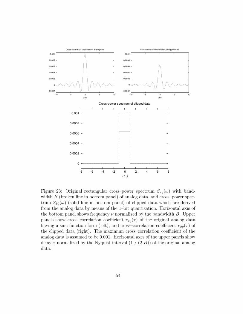
-0.0002

0

0.0002

0.0004

0.0006

0.0008

0.001

-10 -5 0 5 102Bτ

Cross-correlation coefficient of analog data

-0.0002

0

0.0002

0.0004

0.0006

0.0008

0.001

-10 -5 0 5 102Bτ

Cross-correlation coefficient of clipped data

0

0.0002

0.0004

0.0006

0.0008

0.001

-8 -6 -4 -2 0 2 4 6 8ν / B

Cross-power spectrum of clipped data

Figure 23: Original rectangular cross–power spectrum Sxy(ω) with band-width B (broken line in bottom panel) of analog data, and cross–power spec-trum Sxy(ω) (solid line in bottom panel) of clipped data which are derivedfrom the analog data by means of the 1–bit quantization. Horizontal axis ofthe bottom panel shows frequency ν normalized by the bandwidth B. Upperpanels show cross–correlation coefficient rxy(τ) of the original analog datahaving a sinc function form (left), and cross–correlation coefficient rxy(τ) ofthe clipped data (right). The maximum cross–correlation coefficient of theanalog data is assumed to be 0.001. Horizontal axes of the upper panels showdelay τ normalized by the Nyquist interval (1 / (2 B)) of the original analogdata.

54

analog data x and y having a real rectangular cross–power spectrum Sxy(ω)of bandwidth B (broken line in bottom panel). The cross–power spectrum ofthe analog data Sxy(ω) in this Figure is normalized by the geometric mean

of the dispersions√

Rxx(0) Ryy(0), and, therefore, is the Fourier transform of

the cross–correlation coefficient rxy(τ). We assume here that the maximumcross–correlation coefficient of the analog data is small, and, for definiteness,set it to be 0.001. Upper panels of the Figure show (1) cross–correlationcoefficient of the analog data rxy(τ) having a sinc function form (left), and (2)

cross–correlation coefficient of the clipped data rxy(τ) = Rxy(τ) ∼= 2

πrxy(τ)

(right).Unlike in the power spectrum case, the spectrum after clipping remains

rectangular, though peak amplitude is reduced by a factor of 2/π ∼= 0.6366compared with the original analog one, in this cross–power spectrum case.This is because the cross–correlation coefficient of the clipped data is justproportional to the cross–correlation coefficient of the original analog datawith a proportionality coefficient of 2/π, in the approximation of the smallcross–correlation coefficient | rxy(τ) |� 1, which we assumed here.

1.1.23 Price’s Theorem

Now we proceed to the 2–bit quantization case. Although we can derivethe cross–correlation of the 2–bit quantized data by evaluating probabilitiesof quantization states, as we learned in the 1–bit quantization case, use ofPrice’s theorem (Price, 1958) offers a simpler solution.

The theorem states the following.Suppose we have zero–mean stationary random processes x(t) and y(t)

which satisfy joint Gaussian probability density:

f(x, y) ≡ f(x, y; τ) =1

2πσxσy

√1 − r2

e− 1

2(1 − r2)

(

x2

σ2x

− 2 rx y

σx σy+

y2

σ2y

)

,

where σ2x = Rxx(0) and σ2

y = Ryy(0) are dispersions and r ≡ rxy(τ) =Rxy(τ)

σx σy

is a cross–correlation coefficient of the processes x(t) and y(t).Then, for an arbitrary function g(x, y) with expectation

〈g(x, y)〉 =

∞∫

−∞

∞∫

−∞g(x, y)f(x, y) dx dy, (99)

55

we have

1

σnx σn

y

∂n〈g(x, y)〉∂ rn

=⟨

∂2ng(x, y)

∂xn ∂yn

⟩

, (100)

(Price, 1958).

Auxiliary Formula

In order to prove Price’s theorem, we first derive an auxiliary formula(Papoulis, 1984):

1

σnx σn

y

∂nf(x, y)

∂rn=

∂2nf(x, y)

∂xn ∂yn, or

∂nf(x′, y′)

∂rn=

∂2nf(x′, y′)

∂x′n ∂y′n , (101)

where

x′ =x

σx, y′ =

y

σy,

f(x′, y′) =1

2π σx σy

√1 − r2

e−x′2 − 2 r x′ y′ + y′2

2(1 − r2) . (102)

We verify this formula using the method of mathematical induction.

• For n = 1, simple differentiations show

∂f(x′, y′)

∂r=

r (1 − r2) + (r x′ − y′) (r y′ − x′)

2πσx σy (1 − r2)5/2e−x′2 − 2 r x′ y′ + y′2

2(1 − r2) ,

and

∂2f(x′, y′)

∂x′ ∂y′ =r (1 − r2) + (r x′ − y′) (r y′ − x′)

2π σx σy (1 − r2)5/2e−x′2 − 2 r x′ y′ + y′2

2(1 − r2) .

Therefore,∂f(x′, y′)

∂r=

∂2f(x′, y′)

∂x′ ∂y′ , i.e. the formula is valid for n = 1.

• Now, if the formula is valid for n = m:

∂mf(x′, y′)

∂rm=

∂2mf(x′, y′)

∂x′m ∂y′m ,

56

then, for n = m + 1, we have

∂m+1f(x′, y′)

∂rm+1=

∂

∂r

∂mf(x′, y′)

∂rm=

∂

∂r

∂2mf(x′, y′)

∂x′m ∂y′m

=∂2m

∂x′m ∂y′m∂f(x′, y′)

∂r=

∂2m

∂x′m ∂y′m∂2f(x′, y′)

∂x′ ∂y′ =∂2(m+1)f(x′, y′)

∂x′m+1 ∂y′m+1 ,

i.e., the formula is also valid for n = m + 1.

Since the formula is valid for n = 1, this means that the formula isvalid for arbitrary n ≥ 1.

Thus, we confirmed the auxiliary formula.

Proof of Price’s Theorem

We now prove Price’s theorem, using again the method of mathematicalinduction.

• For n = 1, we have

1

σx σy

∂〈g(x, y)〉∂ r

=

∞∫

−∞

∞∫

−∞g

1

σx σy

∂f

∂rdx dy =

∞∫

−∞

∞∫

−∞g

∂2f

∂x ∂ydx dy

=

∞∫

−∞

∞∫

−∞

[

∂

∂x

(

g∂f

∂y

)

− ∂

∂y

(

∂g

∂xf

)

+∂2g

∂x ∂yf

]

dx dy

=

∞∫

−∞

(

g∂f

∂y

)

∣

∣

∣

∣

x=+∞

x=−∞dy −

∞∫

−∞

(

∂g

∂xf

)

∣

∣

∣

∣

y=+∞

y=−∞dx +

∞∫

−∞

∞∫

−∞

∂2g

∂x ∂yf dx dy,

where we used the auxiliary formula:

1

σx σy

∂f(x, y)

∂r=

∂2f(x, y)

∂x ∂y.

First two terms in the RHS vanish as long as g(x, y) e−(x2+y2) convergesto zero at x = ±∞ and y = ±∞. Thus,

1

σx σy

∂〈g(x, y)〉∂ r

=

∞∫

−∞

∞∫

−∞

∂2g(x, y)

∂x ∂yf(x, y) dx dy =

⟨

∂2g(x, y)

∂x ∂y

⟩

,

i.e. the theorem is valid for n = 1.

57

• Now, if the theorem is valid for n = m:

1

σmx σm

y

∂m〈g(x, y)〉∂ rm

=⟨

∂2mg(x, y)

∂xm ∂ym

⟩

,

then, for n = m + 1, we have

1

σm+1x σm+1

y

∂m+1〈g(x, y)〉∂rm+1

=1

σx σy

∂

∂r

(

1

σmx σm

y

∂m〈g(x, y)〉∂ rm

)

=1

σx σy

∂

∂r

⟨

∂2mg(x, y)

∂xm ∂ym

⟩

=

∞∫

−∞

∞∫

−∞

∂2mg(x, y)

∂xm ∂ym

1

σx σy

∂f(x, y)

∂rdx dy

=

∞∫

−∞

∞∫

−∞

∂2mg(x, y)

∂xm ∂ym

∂2f(x, y)

∂x ∂ydx dy.

Integrating by parts again, we see that the last term is equal to

∞∫

−∞

∞∫

−∞

∂2(m+1)g(x, y)

∂xm+1 ∂ym+1f(x, y) dx dy =

⟨

∂2(m+1)g(x, y)

∂xm+1 ∂ym+1

⟩

,

as long as g(x, y) e−(x2+y2) converges to zero at x = ±∞ and y = ±∞.Therefore, the theorem is valid for n = m + 1, and, hence, for anyn ≥ 1.

Thus we proved Price’s Theorem.

Price’s Theorem in the 1–Bit Quantaization Case

Let us experience usefulness of Price’s theorem in the 1–bit quantizationcase as an example. If we choose g(x, y) = x y, then we have

〈g(x, y)〉 = Rxy = 〈x y〉,

with

x(x) =

+1 : x ≥ 0

−1 : x < 0,y(y) =

+1 : y ≥ 0

−1 : y < 0,

in the 1–bit quantization case. We again assume that x and y obey the jointGaussian probability density:

f(x, y) =1

2πσxσy

√1 − r2

e− 1

2(1 − r2)

(

x2

σ2x

− 2 rx y

σx σy

+y2

σ2y

)

.

58

Now, Price’s theorem says

1

σx σy

∂Rxy

∂r=⟨

∂2(x y)

∂x ∂y

⟩

=⟨

∂x

∂x

∂y

∂y

⟩

,

and we have∂x

∂x= 2 δ(x),

∂y

∂y= 2 δ(y),

in the 1–bit quantization case. Therefore

⟨

∂x

∂x

∂y

∂y

⟩

=

∞∫

−∞

∞∫

−∞4 δ(x) δ(y) f(x, y) dx dy =

2

π σx σy

√1 − r2

.

Thus we have∂Rxy

∂r=

2

π√

1 − r2,

and hence

Rxy =2

π

r∫

0

dr′√1 − r′2

=2

πarcsin(r),

where the limits of the integration are chosen to satisfy Rxy = 0 at r = 0.Thus, Price’s theorem allows us to derive the van Vleck relationship in

the really straightforward way.

1.1.24 Cross–Correlation of the 2-Bit Quantized Data

Now we consider, for definiteness, cross–correlation Rxy(τ) of 2–bit quantizeddata x(t) and y(t), though logics below are equally applicable to autocorre-lation as well. Let clipping criteria for the 2–bit quantization are those givenin Figure 17 and Table 1. We assume a simple case where dispersions ofthe original analog data x(t) and y(t) are identical, and denote the commonvalue as σ, i.e. σx = σy = σ. Then, the joint probability density is given by

f(x, y) ≡ f(x, y; τ) =1

2πσ2√

1 − r2e−x2 − 2 r x y + y2

2σ2 (1 − r2) , (103)

where r ≡ rxy(τ) is the cross–correlation coefficient of the analog data.According to Price’s theorem, the cross–correlation of the clipped data

Rxy(τ) satisfies1

σ2

∂Rxy

∂r=⟨

∂2(x y)

∂x ∂y

⟩

=⟨

∂x

∂x

∂y

∂y

⟩

, where the derivatives

59

are now given by

∂x

∂x= (n − 1) δ(x + v0) + 2 δ(x) + (n − 1) δ(x − v0),

∂y

∂y= (n − 1) δ(y + v0) + 2 δ(y) + (n − 1) δ(y − v0).

Using these derivatives, we can calculate

∂Rxy

∂r= σ2

⟨

∂x

∂x

∂y

∂y

⟩

= σ2

∞∫

−∞

∞∫

−∞

∂x

∂x

∂y

∂yf(x, y) dx dy.

After simple manipulations, we obtain

∂Rxy

∂r=

1

π√

1 − r2

{

(n − 1)2

[

e− v2

0σ2(1+r) + e

− v20

σ2(1−r)

]

+ 4(n − 1)e− v2

02σ2(1−r2) + 2

}

.

Therefore, the solution which satisfies a condition Rxy = 0 when r = 0, is

Rxy =1

π

r∫

0

1√1 − r′2

{

(n − 1)2

[

e− v2

0σ2(1+r′) + e

− v20

σ2(1−r′)

]

+4(n − 1)e− v2

0

2σ2(1−r′2) + 2

dr′. (104)

In the limiting case where | r |� 1, the cross–correlation is given by

Rxy =r

π

[

2 (n − 1)2 e−v20

σ2 + 4 (n − 1) e−v20

2σ2 + 2

]

=2 r

π[(n−1) E+1]2, (105)

where we introduced a notation

E ≡ e−v20

2σ2 . (106)

Note that the cross–correlation of the clipped data Rxy(τ) is proportional tothe analog cross–correlation coefficient r = rxy(τ), in this case.

1.1.25 Cross–Correlation Coefficient of the 2–Bit Quantized Data

Now we would like to calculate cross–correlation coefficient rxy(τ) of the 2–bitquantized data. For this purpose, we need their dispersions: σ2

xx = Rxx(0)and σ2

yy = Ryy(0), other than the cross–correlation Rxy(τ).

60

We assumed here that analog data x(t) and y(t) have equal dispersions:Rxx(0) = Ryy(0) = σ2, and therefore they obey identical Gaussian probabilitydensities:

f(x) =1

σ√

2 πe−

x2

2 σ2 , and f(y) =1

σ√

2 πe−

y2

2 σ2 . (107)

Since 4 quantization states in the 2–bit clipped data take values −n, −1,+1, and +n, the joint probabilities of the quantization states of x[n] and x[n](or y[n] and y[n]), taken at the same time, satisfy

P (−n, −n; 0) + P (−1, −1; 0) + P (+1, +1; 0) + P (+n, +n; 0) = 1, (108)

and the dispersion: Rxx(0) = 〈x(t) x(t)〉 =4∑

i=1

xi xi P (xi, xi; 0), must be

Rxx(0) = n2 P (−n, −n; 0) + P (−1, −1; 0)

+ P (+1, +1; 0) + n2 P (+n, +n; 0). (109)

Combining equations (108) and (109), and repeating the same thing for y,we obtain

Rxx(0) = Ryy(0) = Φ + n2 (1 − Φ), (110)

where we introduced a notation:

Φ = P (−1, −1; 0) + P (+1, +1; 0) =1

σ√

2 π

+v0∫

−v0

e−ξ2

2 σ2 dξ. (111)

We used here the explicit form of the probability density in equation (107).Thus, the cross–correlation coefficient of the 2–bit quantized data rxy(τ)

is given by

rxy(τ) =Rxy(τ)

√

Rxx(0) Ryy(0)=

Rxy(τ)

Φ + n2 (1 − Φ)

=1

π [Φ + n2 (1 − Φ)]

rxy(τ)∫

0

1√1 − r′2

{

(n − 1)2

[

e− v2

0σ2(1+r′) + e

− v20

σ2(1−r′)

]

+4(n − 1)e− v2

0

2σ2(1−r′2) + 2

dr′, (112)

as a function of the cross–correlation coefficient of the original analog datar = rxy(τ). This is an analogue of the van Vleck relationship in the 2–bitquantization case.

61

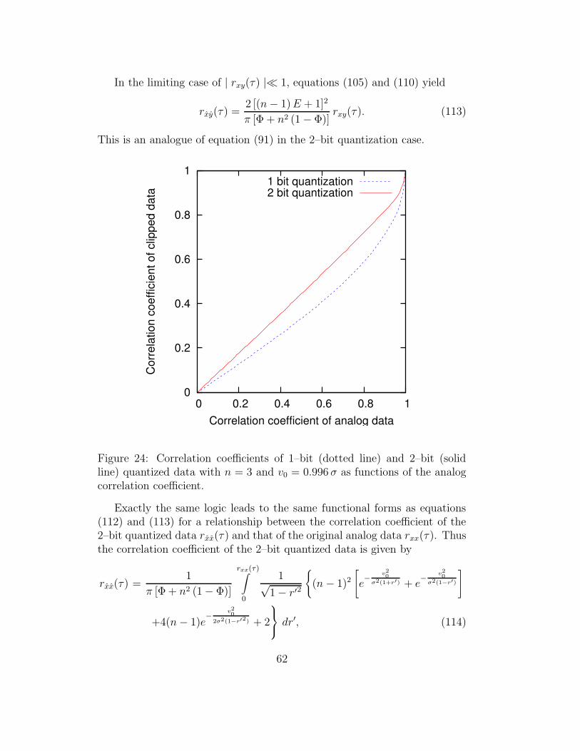
In the limiting case of | rxy(τ) |� 1, equations (105) and (110) yield

rxy(τ) =2 [(n − 1) E + 1]2

π [Φ + n2 (1 − Φ)]rxy(τ). (113)

This is an analogue of equation (91) in the 2–bit quantization case.

0

0.2

0.4

0.6

0.8

1

0 0.2 0.4 0.6 0.8 1

Cor

rela

tion

coef

ficie

nt o

f clip

ped

data


1 bit quantization2 bit quantization

Figure 24: Correlation coefficients of 1–bit (dotted line) and 2–bit (solidline) quantized data with n = 3 and v0 = 0.996 σ as functions of the analogcorrelation coefficient.

Exactly the same logic leads to the same functional forms as equations(112) and (113) for a relationship between the correlation coefficient of the2–bit quantized data rxx(τ) and that of the original analog data rxx(τ). Thusthe correlation coefficient of the 2–bit quantized data is given by

rxx(τ) =1

π [Φ + n2 (1 − Φ)]

rxx(τ)∫

0

1√1 − r′2

{

(n − 1)2

[

e− v2

0σ2(1+r′) + e

− v20

σ2(1−r′)

]

+4(n − 1)e− v2

0

2σ2(1−r′2) + 2

dr′, (114)

62

for a general case, and

rxx(τ) =2 [(n − 1) E + 1]2

π [Φ + n2 (1 − Φ)]rxx(τ), (115)

for the limiting case of | rxx(τ) |� 1.

Figure 24 shows the relationship between the correlation coefficient, whichcould be either (auto–)correlation coefficient or cross–correlation coefficient,of the clipped data and that of the original analog data. The dotted lineshows the van Vleck relationship for the 1–bit quantization case as given byequation (90) or (95). The solid line shows the relationship for the 2–bitquantization case as given by equation (112) or (114) for a particular set ofparameters n = 3 and v0 = 0.996 σ.

1.1.26 Power and Cross–Power Spectra of 2-Bit Quantized Data

We can now calculate power spectrum Sxx(ω) and cross–power spectrumSxy(ω)of the 2–bit quantized data, which are normalized by the dispersion σ2

x andgeometric mean of the dispersions σx σy, respectively, by Fourier transformingthe correlation coefficient rxx(τ) and the cross–correlation coefficient rxy(τ)given in equation (112),

Sxx(ω) =

∞∫

−∞rxx(τ) e−iωτ dτ =

∞∫

−∞F (rxx(τ)) e−iωτ dτ,

Sxy(ω) =

∞∫

−∞rxy(τ) e−iωτ dτ =

∞∫

−∞F (rxy(τ)) e−iωτ dτ, (116)

where the function F (r) is given by

F (r) =1

π (Φ + n2 (1 − Φ)

r∫

0

1√1 − r′2

{

(n − 1)2

[

e− v2

0σ2(1+r′) + e

− v20

σ2(1−r′)

]

+4(n − 1)e− v2

0

2σ2(1−r′2) + 2

dr′.

Let us again consider the case when analog data have rectangular spectra.Figure 25 shows the power spectrum Sxx(ω) of the 2–bit quantized data inthe case with n = 3 and v0 = 0.996 σ (solid line in bottom panel) and that ofthe original analog data Sxx(ω) with the rectangular shape of bandwidth B(broken line in bottom panel). Similarly to the 1–bit case, areas under thespectra (i.e. powers) of the analog and clipped data are equal. Also shownare (1) correlation coefficient of the analog data rxx(τ) having a sinc function

63

-0.2

0

0.2

0.4

0.6

0.8

1

-10 -5 0 5 102Bτ


-0.2

0

0.2

0.4

0.6

0.8

1

-10 -5 0 5 102Bτ

Correlation coefficient of 2-bit quantized data

0

0.2

0.4

0.6

0.8

1

-8 -6 -4 -2 0 2 4 6 8ν / B

Power spectrum of 2-bit quantized data

Figure 25: Original rectangular power spectrum Sxx(ω) with bandwidth B(broken line in bottom panel) of the analog data, and power spectrum Sxx(ω)(solid line in bottom panel) of the 2–bit quantized data with n = 3 and v0 =0.996 σ . Horizontal axis of the bottom panel shows frequency ν normalizedby the bandwidth B. Upper panels show correlation coefficient rxx(τ) ofthe original analog data having a sinc function form (left), and correlationcoefficient rxx(τ) of the 2–bit quantized data (right). Horizontal axes of theupper panels show delay τ normalized by the Nyquist interval (1 / (2 B)) ofthe original analog data.

64

-0.0002

0

0.0002

0.0004

0.0006

0.0008

0.001

-10 -5 0 5 102Bτ

Cross-correlation coefficient of analog data

-0.0002

0

0.0002

0.0004

0.0006

0.0008

0.001

-10 -5 0 5 102Bτ

Cross-correlation coefficient of 2-bit quantized data

0

0.0002

0.0004

0.0006

0.0008

0.001

-8 -6 -4 -2 0 2 4 6 8ν / B

Cross-power spectrum of 2-bit quantized data

Figure 26: Original rectangular cross–power spectrum Sxy(ω) with band-width B (broken line in bottom panel) of the analog data, and cross–powerspectrum Sxy(ω) (solid line in bottom panel) of the 2–bit quantized data withn = 3 and v0 = 0.996 σ . Horizontal axis of the bottom panel shows frequencyν normalized by the bandwidth B. Upper panels show cross–correlation co-efficient rxy(τ) of the original analog data having a sinc function form (left),and cross–correlation coefficient rxy(τ) of the 2–bit quatized data (right).The maximum cross–correlation coefficient of the analog data is assumed tobe 0.001. Horizontal axes of the upper panels show delay τ which is normal-ized by the Nyquist interval (1 / (2 B)) of the original analog data.

65

form (upper left panel), and (2) correlation coefficient of the 2–bit quantizeddata rxx(τ) (upper right panel).

The spectrum after clipping again shows somewhat reduced peak ampli-tude and a low–level skirt extending over a wide range of frequency. Thus,the original Nyquist interval (1 / (2B)) is not strictly optimum for samplingthe clipped data again, though to a smaller extent compared with the 1–bitcase.

On the other hand, Figure 26 shows a cross–power spectrum Sxy(ω) of the2–bit quantized data x and y in the case with n = 3 and v0 = 0.996 σ (solidline in bottom panel) and that of the original analog data x and y, having areal rectangular cross–power spectrum Sxy(ω) of bandwidth B (broken line inbottom panel). We assumed here again that the maximum cross–correlationcoefficient of the analog data is as small as 0.001, for definiteness. Upperpanels of the Figure show (1) cross–correlation coefficient of the analog datarxy(τ) having a sinc function form (left), and (2) cross–correlation coefficientof the clipped data rxy(τ) (right). Note that the spectrum after clippingremains again rectangular, because of the approximate linearity between theanalog and clipped cross–correlation coefficients.

1.1.27 Dispersion of Digital Correlator Output

Let us now examine the signal–to–noise ratio of an output of a digital corre-lator. How does the S/N ratio differ from the one expected from the analogor “semi–analog” correlator, which we saw earlier? For this purpose, we firstconsider dispersion of the digital correlator output.

The output R of a digital correlator, which averages products of N sam-ples of clipped data x[i] and y[i] from two antennas in a radio interferometer,is

R =1

NN∑

i=1

x[i] y[i]. (117)

We again assume here that the delay tracking and the fringe stopping arecompletely performed before the multiplication, so that signal parts in thetwo data streams x[i] and y[i] are perfectly aligned.

Under the assumption of the stationary random processes, the expecta-tion 〈R〉 and the dispersion σ2

R of the output R are given by

〈R〉 = 〈x[i] y[i]〉 = Rxy[0], (118)

σ2R = 〈R2〉 − 〈R〉2 =

1

N 2

N∑

i=1

N∑

j=1

〈x[i] y[i] x[j] y[j]〉 − R2xy[0]. (119)

66

Note that usually N is a huge number. For example, if we integrate datasampled with a rate of 4 Msps (mega sample per second) for 1 second, thenN ≈ 4, 000, 000.

Let us assume that the original analog data x(t) and y(t) have rectangularbaseband spectra with bandwith B, and the data are sampled with Nyquistrate 2B. In such a case, different sample pairs are independent in the analogdata, as we discussed earlier, i.e. Rxy[m], Rxx[m], and Ryy[m] are all zero,if m 6= 0. The same statement is valid for the 1–bit quantized and 2–bitquantized data, since correlation coefficients, and correlations, too, of theseclipped data are equal to zero when those of the original analog data arezero, as we can easily see in equations (90), (95), and (112). Thus, Rxy[m],Rxx[m], and Ryy[m] are also all zero, if m 6= 0. In addition, we assume thatthe cross–correlation Rxy[0] is much smaller than the autocorrelations Rxx[0]and Ryy[0], as usually so in radio interferometers.

Then in the double sum of equation (119):

N∑

i=1

N∑

j=1

〈x[i] y[i] x[j] y[j]〉 =N∑

i=1

〈x[i] y[i] x[i] y[i]〉 +N∑

i=1

N∑

j 6=i

〈x[i] y[i] x[j] y[j]〉,

(120)dominating terms will be

N∑

i=1

N∑

j=1

〈x[i] y[i] x[j] y[j]〉 ∼=N∑

i=1

〈x[i] x[i]〉〈y[i] y[i]〉 +N∑

i=1

N∑

j 6=i

〈x[i] y[i]〉〈x[j] y[j]〉

= N Rxx[0] Ryy[0] + N (N − 1) R2xy[0] ∼= N Rxx[0] Ryy[0] + N 2 R2

xy[0],

(121)

where we neglected 1 compared with the large number N .Now equations (119) and (121) yeild an approximate formula for the

dispersion of the digital correlator output:

σ2R∼= 1

N Rxx[0] Ryy[0] + R2xy[0] − R2

xy[0] =1

N Rxx[0] Ryy[0]. (122)

1.1.28 S/N Ratio of Digital Correlator Output

We are now ready to calculate the signal 〈R〉 to noise σR ratio SNR of thedigital correlator output, using equation (122). We obtain

SNR =〈R〉σR

=√N Rxy[0]√

Rxx[0] Ryy[0]=

√N rxy[0] =

√N rxy[0]

rxy[0]ρ, (123)

where ρ ≡ rxy[0] is the maximum cross–correlation coefficient of the originalanalog data under our assumption of the perfect delay tracking and fringe

67

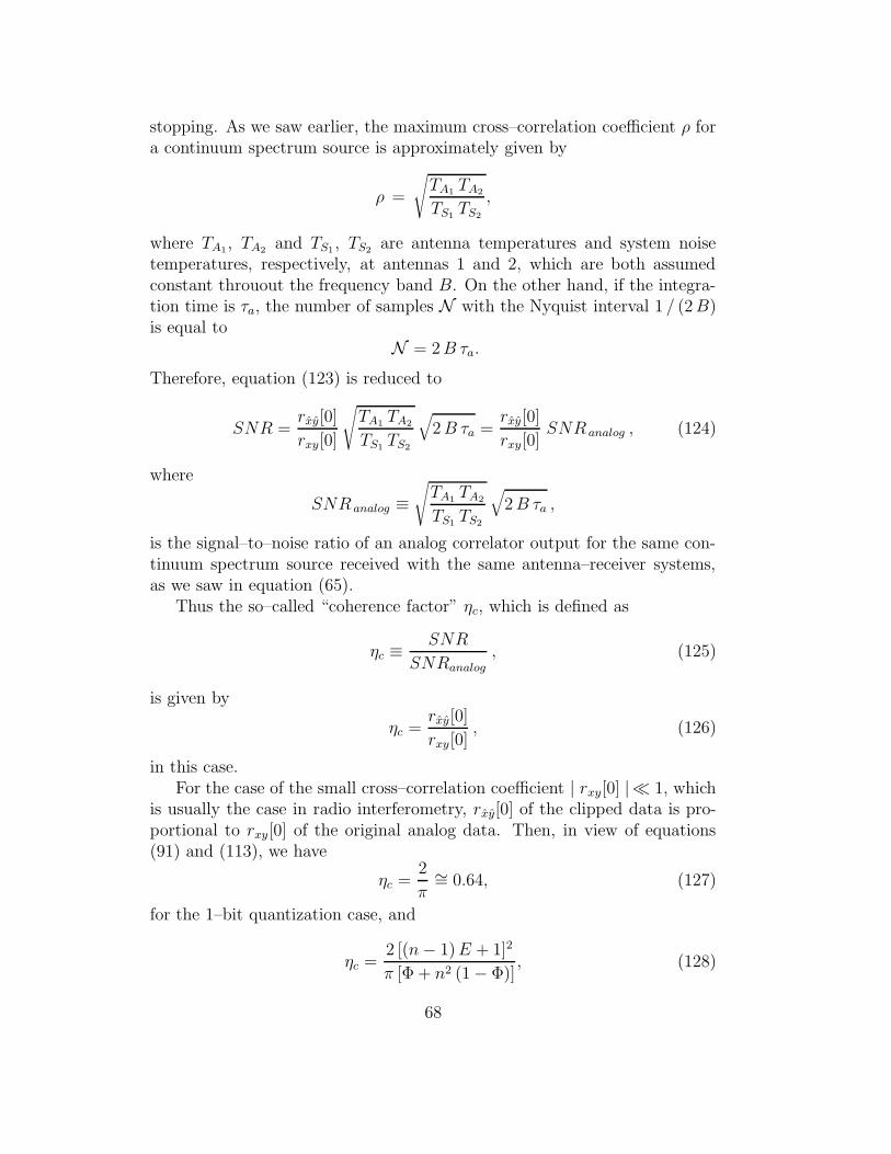
stopping. As we saw earlier, the maximum cross–correlation coefficient ρ fora continuum spectrum source is approximately given by

ρ =

√

TA1 TA2

TS1 TS2

,

where TA1, TA2 and TS1 , TS2 are antenna temperatures and system noisetemperatures, respectively, at antennas 1 and 2, which are both assumedconstant throuout the frequency band B. On the other hand, if the integra-tion time is τa, the number of samples N with the Nyquist interval 1 / (2 B)is equal to

N = 2 B τa.

Therefore, equation (123) is reduced to

SNR =rxy[0]

rxy[0]

√

TA1 TA2

TS1 TS2

√

2 B τa =rxy[0]

rxy[0]SNR analog , (124)

where

SNR analog ≡√

TA1 TA2

TS1 TS2

√

2 B τa ,

is the signal–to–noise ratio of an analog correlator output for the same con-tinuum spectrum source received with the same antenna–receiver systems,as we saw in equation (65).

Thus the so–called “coherence factor” ηc, which is defined as

ηc ≡SNR

SNRanalog

, (125)

is given by

ηc =rxy[0]

rxy[0], (126)

in this case.For the case of the small cross–correlation coefficient | rxy[0] |� 1, which

is usually the case in radio interferometry, rxy[0] of the clipped data is pro-portional to rxy[0] of the original analog data. Then, in view of equations(91) and (113), we have

ηc =2

π∼= 0.64, (127)

for the 1–bit quantization case, and

ηc =2 [(n − 1) E + 1]2

π [Φ + n2 (1 − Φ)], (128)

68

for the 2–bit quantization case.With the coherence factor ηc, equation (124) is reduced to

SNR = ηc

√

TA1 TA2

TS1 TS2

√

2 B τa, (129)

which is an important formula for estimating sensitivity of a radio interfer-ometer observing a continuum spectrum source. Note that the coherencefactor as given by equation (126) still takes into account only the loss dueto effects of clipping. Usually, the factor is further reduced in view of lossesoccuring through digital processing in hardware correlators.

1.1.29 Optimum Parameters v0 and n in the 2–Bit Quantization

We mentioned earlier that the two parameters in the 2–bit quantization, thethreshold v0 and the higher–level value n, are chosen so that the signal–to–noise ratio of the digital correlator output is maximized. This condition is

2.5 3

3.5 4

4.5 0.8 0.85

0.9 0.95

1 1.05

1.1 1.15

0.86

0.865

0.87

0.875

0.88

0.885

Coherence factor of 2-bit quantized data

n

v0 / σ

Figure 27: Coherence factor of the 2–bit quantized data as a function ofnormalized threshold v0/σ and higher–level value n in the limiting case ofthe small cross–correlation coefficient.

69

fulfilled when the coherence factor ηc takes the maximum. In the limiting caseof the small cross–correlation coeficient | rxy[0] |� 1, which is common inradio interferometry, we can calculate the coherence factor ηc using equation(128) with explicit forms for the functions E and Φ given in equations (106)and (111).

Figure 27 shows the coherece factor as a function of the two parameters, v0

normalized by the analog dispersion σ, and n, in the small cross–correlationcoefficient case.

As we see from the Figure, the maximum value of the coherence factorηc = 0.883 is obtained when n = 3.34 and v0 = 0.982 σ. However, froma practical point of view, designing of digital circuitry for 2–bit hardwarecorrelators can be more easily implemented when n is an integer. Therefore,n = 3, v0 = 0.996 σ with ηc = 0.881, and n = 4, v0 = 0.942 σ with ηc = 0.880,are often used in existing VLBI 2–bit quantization systems. This is why weadopted n = 3, v0 = 0.996 σ in Figures 24, 25, and 26.

Accordingly, in the limiting case of the small cross–correlation coefficient| rxy[0] |� 1, the coherence factor, which takes into acount the effect ofclipping only, is given by

ηc∼= 0.64, (130)

for the 1–bit quantization case, and

ηc∼= 0.88, (131)

for the 2–bit quantization case.

1.1.30 Effect of Oversampling in S/N Ratio of Clipped Data

As we saw earlier, power spectra of clipped data show low–level but broadskirt beyond band edges at ν = ±B of the original rectangular spectra ofcorresponding analog data (Figures 22 and 25). Therefore, the Nyquist sam-pling for the original analog data with 2B rate is no longer optimum for theclipped data.

Sampling with a rate higher than the Nyquist rate for the analog data 2B,which is a little incorrectly called the “oversampling”, improves the signal–to–noise ratio of the clipped data. In this case, different sample points are nolonger independent any more, and we have to take into account contributionsof autocorrelations between different sample points, i.e. Rxx[m] and Ryy[m]with m 6= 0, when we calculate the signal–to–noise ratio.

Let us consider that we sample our data with a rate which is β times asfast as the Nyquist rate of the original band–limited analog data 2B. Then,in the calculation of the dispersion of the digital correlator output R shown

70

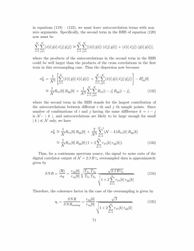
in equations (119) – (122), we must leave autocorrelation terms with non–zero arguments. Specifically, the second term in the RHS of equation (120)now must be

N∑

i=1

N∑

j 6=i

〈x[i] y[i] x[j] y[j]〉 ∼=N∑

i=1

N∑

j 6=i

[〈x[i] y[i]〉〈x[j] y[i]〉 + 〈x[i] x[j]〉〈y[i] y[i]〉],

where the products of the autocorrelations in the second term in the RHScould be well larger than the products of the cross–correlations in the firstterm in this oversampling case. Thus the dispersion now becomes

σ2R =

1

N 2

N∑

i=1

〈x[i] y[i] x[i] y[i]〉 +N∑

i=1

N∑

j 6=i

〈x[i] y[i] x[j] y[j]〉

− R2xy[0]

∼= 1

N Rxx[0] Ryy[0] +1

N 2

N∑

i=1

N∑

j 6=i

Rxx[i − j] Ryy[i − j], (132)

where the second term in the RHS stands for the largest contribution ofthe autocorrelations between different i–th and j–th sample points. Sincenumber of combinations of i and j having the same diffference k = i − jis N− | k |, and autocorrelations are likely to be large enough for small| k |� N only, we have

σ2R∼= 1

N Rxx[0] Ryy[0] +2

N 2

N−1∑

k=1

(N − k)Rxx[k] Ryy[k]

∼= 1

N Rxx[0] Ryy[0] (1 + 2∞∑

k=1

rxx[k] ryy[k]). (133)

Thus, for a continuum spectrum source, the signal–to–noise ratio of thedigital correlator output of N = 2 β B τa oversampled data is approximatelygiven by

SNR =〈R〉σR

=rxy[0]

rxy[0]

√

TA1 TA2

TS1 TS2

√2 β B τa

√

√

√

√1 + 2∞∑

k=1

rxx[k] ryy[k]

. (134)

Therefore, the coherence factor in the case of the oversampling is given by

ηc =SNR

SNRanalog=

rxy[0]

rxy[0]

√β

√

√

√

√1 + 2∞∑

k=1

rxx[k] ryy[k]

. (135)

71

We can estimate this factor, using equations (95) and (114) which describecorrelation coefficients of the clipped data rxx[k] and ryy[k] as functions ofanalog correlation coefficients rxx[k] and ryy[k], which we denote as rxx[k] =fcl(rxx[k]) and ryy[k] = fcl(ryy[k]). Here fcl is the clipping function which isgiven in equation (95) and equation (114) for the 1–bit and 2–bit quatizationcases, respectively.

When the original analog data have rectangular baseband spectra withbandwidth B, as we have assumed in the present discussion, the analogcorrelation coefficients rxx(τ) and ryy(τ) have sinc function forms:

rxx(τ) = ryy(τ) =sin(2π B τ)

2π B τ,

as given in equation (46). Therefore, correlation coefficients of their timesamples x[k] and y[k] with the sampling interval Ts = 1/(2 B β) are given by

rxx[k] = ryy[k] = rxx(k Ts) = ryy(k Ts) =sin

(

π kβ

)

π kβ

. (136)

0

0.2

0.4

0.6

0.8

1

0 2 4 6 8 10 12 14 16 18 20

η c

β

Coherence Factor vs Oversampling Ratio

analogtwo-bitone-bit

Figure 28: Coherence factor ηc for the analog (+), 2–bit quantized (×), and1–bit quantized (∗) data as functions of the oversampling ratio β.

Thus, the signal–to–noise ratio and the coherence factor of the oversam-pled clipped data is given by

SNR = ηc

√

TA1 TA2

TS1 TS2

√

2 B τa, (137)

72

ηc =rxy[0]

rxy[0]

√β

√

√

√

√

√1 + 2∞∑

k=1

f 2cl

sin(

π kβ

)

π kβ

. (138)

Figure 28 shows the coherence factor ηc for the analog, 2–bit quantized,and 1–bit quantized data as functions of the oversampling ratio β, calculatedby means of equation (138). The coherence factor of the clipped data im-proves gradually with increasing β, approaching to some constant values. Onthe other hand, the coherence factor of the analog data is always 1, irrespec-tive of the oversampling ratio β, in accordance with the sampling theorem.

In a particular case of the “double–speed sampling” β = 2, we have ηc =0.744 for the 1–bit quantized data, and ηc = 0.930 for the 2–bit quantizeddata.

1.1.31 Coherence Factor and Sensitivity with Given Bit Rate

Coherence factor ηc with different clipping and oversampling is summarizedin Table 2. It is obvious that the coherence factor increases as we increase

Number of Number of coherence factor ηc

bits Nb quantization levels β = 1 β = 2

1 2 0.64 0.74

2 4 0.88 0.93

Table 2: Relationship of coherence factor ηc with number of bits Nb andoversampling ratio β.

the number of bits Nb and the oversampling ratio β.However, actual observations are usually limited by maximum bit–rate

νb of data streams allowed by correlators or recorders. If the maximum bit–rate νb is fixed, the maximum permissible sampling rate, which is β times aslarge as the Nyquist rate 2B with the analog bandwidth B, is νb/Nb = 2 β B.Therefore, the maximum allowable bandwidth is limited by the bit–rate asB = νb/(2 β Nb). Hence, in view of equation (137), the maximum signal–to–noise ratio, i.e. the sensitivity of the interferometric observation, for acontinuum spectrum source, is proportional to

SNR ∝ ηc

√B ∝ ηc√

βNb

. (139)

73

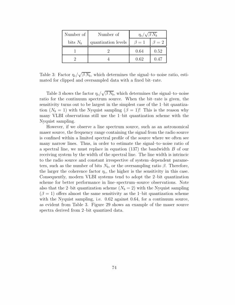
Number of Number of ηc/√

β Nb

bits Nb quantization levels β = 1 β = 2

1 2 0.64 0.52

2 4 0.62 0.47

Table 3: Factor ηc/√

β Nb, which determines the signal–to–noise ratio, esti-mated for clipped and oversampled data with a fixed bit–rate.

Table 3 shows the factor ηc/√

β Nb, which determines the signal–to–noiseratio for the continuum spectrum source. When the bit–rate is given, thesensitivity turns out to be largest in the simplest case of the 1–bit quantiza-tion (Nb = 1) with the Nyquist sampling (β = 1)! This is the reason whymany VLBI observations still use the 1–bit quantization scheme with theNyquist sampling.

However, if we observe a line spectrum source, such as an astronomicalmaser source, the frequency range containing the signal from the radio sourceis confined within a limited spectral profile of the source where we often seemany narrow lines. Thus, in order to estimate the signal–to–noise ratio ofa spectral line, we must replace in equation (137) the bandwidth B of ourreceiving system by the width of the spectral line. The line width is intrincicto the radio source and constant irrespective of system–dependent parame-ters, such as the number of bits Nb, or the oversampling ratio β. Therefore,the larger the coherence factor ηc, the higher is the sensitivity in this case.Consequently, modern VLBI systems tend to adopt the 2–bit quantizationscheme for better performance in line–spectrum–source observations. Notealso that the 2–bit quantization scheme (Nb = 2) with the Nyquist sampling(β = 1) offers almost the same sensitivity as the 1–bit quantization schemewith the Nyquist sampling, i.e. 0.62 against 0.64, for a continuum source,as evident from Table 3. Figure 29 shows an example of the maser sourcespectra derived from 2–bit quantized data.

74

Figure 29: Spectra of the water maser source Cep A in an active region ofstar formation derived from 2–bit quantized data. Upper panel shows total–power spectrum with Mizusawa 20m antenna, and lower panel shows phaseand amplitude of cross–power spectrum with Mizusawa–Ogasawara baselineof the VERA. Profiles of the two spectra are fairly different which indicateeffects of partial resolution of maser features in the VLBI baseline. Notethat amplitude scales are different in the two panels. (T. Hirota, privatecommunication in 2005.)

75

1.2 Frequency Standard

1.2.1 VLBI Requires “Absolute” Frequency Stability

Multiplier Integrator

Multiplier Integrator

Tape recorder

analog digital

instrumental delay

correlator

correlator

Connected Interferometer

VLBI

RF IF ν ν - ν0

Figure 30: Connected–Element Interferometer vs. VLBI system.

Development of the highly stable frequency standard was indispensablefor realization of VLBI.

In the case of the connected–element interferometer, a common frequencystandard is used to generate local oscillator (LO) reference signals for fre-quency conversion in all antennas (see upper panel of Figure 30). Therefore,any phase noise, due to instability in the frequency standard, is common inthe signals from all antennas. Such common phase noise from any given an-tenna is always compensated by the same phase noise from another antenna,in the correlation processing.

In fact, let us assume that a signal from a radio source, which we assumeto be point–like for simplicity, received by antenna A is:

vA(t) ∝ sin[ωt − φ(t)],

and the same signal received by antenna B is:

vB(T ) ∝ sin[ω(t − τg) − φ(t)],

76

where ω is a frequency of the radio signal, τg is the geometric delay betweenthe two antennas, and φ(t) is the common phase noise due to the frequencystandard.

After multiplication of these signals, we have

vA(t) vB(t) ∝ 1

2{cos(ωτg) − cos[2 ωt − ωτg − 2 φ(t)]},

and after integration (averaging), we have

〈vA(t) vB(t)〉 ∝ 1

2cos(ωτg), (140)

since rapidly oscillating second term with frequency 2 ω is averaged out.Thus, no effect of the phase noise remains in the correlator output! Con-

sequently, correlation results in connected–element interferometersare almost unaffected by the instability of the frequency standard.Then, we readily obtain the almost pure fringe pattern ∝ cos(ωτg) in thecrorrelation results as shown in equation (140), as far as we perform suffi-ciently long integration to suppress the thermal noise occuring in receivingsystems and in the environment, and achieve high enough signal–to–noise ra-tio. This is why very high stability of frequency standards is not necessarilyrequired in connected–element interferometers.

How about VLBI, then?Each antenna in VLBI uses its own independent frequency standard to

generate the LO reference signal (see lower panel of Figure 30).Then, a signal from a point–like radio source received by antenna A is

given byvA(t) ∝ sin[ωt − φA(t)],

and the same signal received by antenna B is:

vB(t) ∝ sin[ω(t − τg) − φB(t)],

where φA(t) and φB(t) are phase noises in independent frequency standards.After multiplication, we have

vA(t) vB(t) ∝ 1

2{cos[ωτg − φA(t) + φB(t)] − cos[2 ωt − ωτg − φA(t) − φB(t)]},

and after integration (averaging),

〈vA(t) vB(t)〉 ∝ 1

2cos[ωτg − φA(t) + φB(t)]. (141)

77

Therefore, no compensation of the phase noises is expected in the correlatoroutput of VLBI. In other words, correlation results in VLBI are alwaysdirectly affected by the instability of the frequency standards!

The noise in the fringe phase (the argument of the sinusoidal fringe pat-tern in equation (141)) gives rise to two difficulties in VLBI.

First, the fringe phase, which is the important observable in radio inter-ferometry, is contaminated by the phase noise.

Second, the phase noise severely limits the sensitivity of VLBI. Indeed, itbecomes impossible for us to completely stop the oscillation of the sinusoidalfringe pattern if the phase noise varies in time, even when we ideally compen-sate the geometric delay τg by applying accurate enough delay tracking andfringe stopping. Then, if we further integrate (time–average) the correlatoroutput, hoping to get higher signal–to–noise ratio, the phase–noise–inducedoscillation of the fringe pattern results in smaller amplitude of the averagedsignal. The thermal noise contribution in the correlator output must besurely suppressed by the integration, but the averaged signal itself could bereduced even more rapidly due to the oscillation. Depending on the ratiobetween the integration time and the timescale of the oscillation, the inte-gration may not improve the signal–to–noise ratio at all, but even degradeit. Such an effect is called the “coherence loss”. Therefore, the integrationtime must be short enough not to cause large coherence loss, but this impliesthat the signal–to–noise ratio must be limited by the short integration time.

This is why we need “absolute” stability of frequency standards in VLBI,in order to ease these difficulties.

Of cource, not only the noise due to the frequency standards, but anyother phase noise, due for example to the propagation delay through theturbulent atmosphere, causes similar difficulties, as we will see later.

Now we would like to discuss the way to quantitatively describe the fre-quency stability, and to estimate effects of the incomplete stability.

1.2.2 How to Describe Frequency Stability?

Let us consider a reference signal v(t) which is expected to have a form inan ideal case:

v(t) = v0 cos(ω0 t), (142)

with a nominal frequency ω0. In actuality, however, any real reference signalhas a phase noise φ(t), and therefore has a form:

v(t) = v0 cos(ω0 t + φ(t)). (143)

78

In this actual case, instantaneous frequency ωa(t) will be

ωa(t) = ω0 +dφ(t)

dt. (144)

We then introduce a concept of the “fractional frequency deviation(FFD)” y(t), which is defined by

y(t) =δω(t)

ω0=

ωa(t) − ω0

ω0=

1

ω0

dφ(t)

dt, (145)

as a measure of the frequency stability.Let us assume that φ(t) and y(t) are stationary random processes. Then,

their autocorrelations are functions of the time difference τ :

Rφφ(τ) = 〈φ(t + τ) φ(t)〉, and Ryy(τ) = 〈y(t + τ) y(t)〉, (146)

and their power spectra are given by Fourier transform relations:

Sφφ(ω) =

∞∫

−∞Rφφ(τ) e−iωτ dτ, Rφφ(τ) =

1

2π

∞∫

−∞Sφφ(ω) eiωτ dω,

Syy(ω) =

∞∫

−∞Ryy(τ) e−iωτ dτ, Ryy(τ) =

1

2π

∞∫

−∞Syy(ω) eiωτ dω. (147)

In view of equation (145), the autocorrelations of y(t) and φ(t) are mu-tually related by

Ryy(t, t′) = 〈y(t) y(t′)〉 =

1

ω20

⟨

dφ(t)

dt

dφ(t′)

dt′

⟩

=1

ω20

∂2

∂t ∂t′Rφφ(t, t

′). (148)

In our case of the stationary random processes, this is reduced to

Ryy(τ) = − 1

ω20

d2

dτ 2Rφφ(τ), (149)

where τ = t − t′.From equations (147) and (149), we have

Ryy(τ) = − 1

ω20

d2

dτ 2

1

2π

∞∫

−∞Sφφ(ω) eiωτ dω =

1

2π

∞∫

−∞

ω2

ω20

Sφφ(ω) eiωτ dω,

and, therefore, the power spectra of y(t) and φ(t) are related to each otherby a relation:

Syy(ω) =ω2

ω20

Sφφ(ω). (150)

79

Let us make a comment here about conventions which have been tradi-tionally used for describing power spectra in frequency stability discussions.

Since y(t) and φ(t) are real functions of time, the autocorrelation Rφφ(τ)and Ryy(τ), and power spectra Sφφ(ω), Syy(ω) are all real and even functionsof τ and ω. Using this property, and using frequency ν instead of angularfrequency ω = 2π ν, we can describe the power spectra in the “single–sidedforms” Sφφ(ν) and Syy(ν), which have been widely used in the frequencystability discussions:

Sφφ(ν) = 4

∞∫

0

Rφφ(τ) cos(2π ν τ) dτ, Rφφ(τ) =

∞∫

0

Sφφ(ν) cos(2π ν τ) dν,

Syy(ν) = 4

∞∫

0

Ryy(τ) cos(2π ν τ) dτ, Ryy(τ) =

∞∫

0

Syy(ν) cos(2π ν τ) dν.

(151)

These single–sided spectra Sφφ(ν) and Syy(ν) are related to our double–sidedpower spectra Sφφ(ω) and Syy(ω) by:

Sφφ(ν) = 2 Sφφ(2πν), and Syy(ν) = 2 Syy(2πν), (152)

for the positive frequency range ν ≥ 0. Therefore, their mutual relationshiphas been often given by:

Syy(ν) =ν2

ν20

Sφφ(ν), (153)

instead of equation (150), where ν0 =ω0

2π.

However, we will continue to use our double–sided power spectrum formsin equations (147), following our previous discussions.

1.2.3 Types of Phase and Frequency Noises

Measurements have shown that noises in the frequency stability are classi-fied into following types according to the power–law index α of the powerspectrum of the FFD Syy(ω) = Hα ωα with roughly constant coefficients Hα.Each noise type, or power–law component of the FFD spectrum, has its owncharacteristic name listed in Table 4.

An oscillator in a frequency standard often shows a combination of allpower–law components of Table 4 in various frequency ranges, as shownschematically in Figure 31.

80

α Name of Noise Type Syy(ω) Sφφ(ω)

2 White phase H2 ω2 ω20 H2

1 Flicker phase H1 ω1 ω20 H1 ω−1

0 White frequency H0 ω20 H0 ω−2

-1 Flicker frequency H−1 ω−1 ω20 H−1 ω−3

-2 Random walk of frequency H−2 ω−2 ω20 H−2 ω−4

Table 4: Power–law types of phase and frequency noise spectra.

α=2

α=1

α=0

α=−1

α=−2

Figure 31: A schematic spectrum of the FFD, y(t), of an oscillator showingall power–law components in Table 4 in various frequency ranges. Horizontaland vertical axes show the angular frequency ω and the power spectrumSyy(ω), respectively, in log–scales.

81

1.2.4 Time Domain Measurements

It has traditionally been easier to make measurements in the time domain,than in the frequency domain. Hence, frequency stability characteristics areusually given in terms of the time domain measurements.

Suppose that we have N phase values: φ(t1), φ(t2), · · · , φ(tk), · · · , φ(tN ),measured at equally spaced time points: t1, t2, · · · , tk, · · · , tN , with timeinterval T , where T = tk+1 − tk for any k.

Then, using these phase values measured in the time domain, we form adiscrete time series of the “mean fractional frequency deviation” y[k]which is defined by

y[k] =φ(tk+1) − φ(tk)

ω0 T=

1

ω0 T

tk+1∫

tk

dφ(t′)

dt′dt′ =

1

T

tk+1∫

tk

y(t′)dt′, (154)

and can be described also as

y[k] =1

T

t+T2

∫

t−T2

y(t′)dt′, (155)

where t = tk + T /2. This is a running mean of the FFD y(t) at the pointt = tk + T /2 over the time interval T . Thus, y[k] for any k is given by alinear system of y(t):

y[k] = y(t) ∗ a(t) =

∞∫

−∞y(t − t′) a(t′) dt′, (156)

with an impulse response a(t):

a(t) =

1T if − T

2< t ≤ T

2,

0 otherwise,(157)

at t = tk + T /2, similarly to what we saw in Chapter 3.

1.2.5 “True Variance” and “Allan Variance” of Fractional Fre-quency Deviation

Using the mean fractional frequency deviation y[k], which is obtained byaveraging the FFD y(t) for the time interval T , as shown in equation (155),

82

we introduce the “true variance of the fractional frequency deviation(TVAR)” as a function of the time interval T :

I2(T ) = 〈y2[k]〉, (158)

where, we assumed zero–mean of the mean FFD y[k]:

〈y[k]〉 = 0.

In view of the ergodicity, we can estimate the TVAR I2(T ) by means of atime–average Σt of N − 1 values of the squared mean FFD y2[k]:

Σt =1

N − 1

N−1∑

k=1

y2[k]. (159)

Generally speaking, there seems no difficulty in calculating the time–average Σt, and, therefore, this estimated TVAR appears a good measureof the frequency stability. In actuality, however, Σt, as given in equation(159), diverges for some important types of frequency noises, and thereforecannot be used for characterizing the frequency stability as a whole. Theassumption of the stationary random process, or the ergodicity, is not likelyto be strictly fulfilled in these diverging cases.

In order to overcome this difficulty, David W. Allan proposed to take adifference of successive two samples:

∆y[k] = y[k + 1] − y[k], (160)

and calculate an average of the squared difference (∆y[k])2 divided by two:

Σa =1

2 (N − 2)

N−2∑

k=1

(∆y[k])2, (161)

(Allan, 1966). In view of equation (154), the two sample difference ∆y[k] ofthe mean FFD is easily derived from the measured phase noise φ[k] by

∆y[k] =φ(tk+2) − 2 φ(tk+1) + φ(tk)

ω0 T. (162)

The mean square sum Σa gives an estimation of the “two–sample vari-ance” or “Allan variance (AVAR)”:

σ2y(T ) =

〈(∆y[k])2〉2

, (163)

83

τ

τ

y[k]

∆y[k]=y[k+1]-y[k]

Figure 32: Mean square sum of the two–sample difference of the mean FFD(lower panel) has a better chance to converge than that of the mean FFDitself (upper panel), even when the mean FFD shows a diverging long–time–scale behaviour.

as a function of the time interval T .Estimation of the AVAR with Σa has a better chance to converge than

that of the TVAR with Σt, as schematically illustrated in Figure 32. There-fore, the estimated AVAR is widely accepted as a good measure of the fre-quency stability.

In view of equation (154), we can describe the two–sample difference ofthe mean FFD ∆y[k] through time integrations of the FFD y(t):

∆y[k] = y[k + 1] − y[k] =1

T

tk+2∫

tk+1

y(t′) dt′ −tk+1∫

tk

y(t′) dt′

=1

T

t+T∫

t

y(t′) dt′ −t∫

t−Ty(t′) dt′

, (164)

where t = tk+1. This is nothing but a linear system of the FFD y(t):

∆y[k] = y(t) ∗ b(t) =

∞∫

−∞y(t − t′) b(t′) dt′, (165)

with an impulse response:

b(t) =

1T if − T < t ≤ 0,

− 1T if 0 < t ≤ T ,

0 otherwise,

(166)

84

at time t = tk+1.

1.2.6 True Variance and Allan Variance through Power Spectrumof Fractional Frequency Deviation

Equations (156) and (165) describe the discrete–time series y[k] (the meamFFD) and ∆y[k] (the two–sample difference of the mean FFD) through thelinear systems with impulse responses a(t) and b(t) at times t = tk + T /2and t = tk+1, respectively. We can formally extend these linear systems toyield continuous–time functions y(t) and ∆y(t):

y(t) = y(t) ∗ a(t) =

∞∫

−∞y(t − t′) a(t′) dt′,

∆y(t) = y(t) ∗ b(t) =

∞∫

−∞y(t − t′) b(t′) dt′, (167)

at arbitrary time t, and introduce their autocorrelations

Ryy(τ) = 〈y(t + τ) y(t)〉,R∆y∆y(τ) = 〈∆y(t + τ) ∆y(t)〉, (168)

and power spectra Syy(ω) and S∆y∆y(ω). Of course, y(t) takes the particularvalue y[k] at t = tk + T /2, and ∆y(t) takes the particular value of ∆y[k] att = tk+1, i.e.

y(t) = y[k] at t = tk +T2

,

∆y(t) = ∆y[k] at t = tk+1. (169)

Then, we can describe the TVAR, I2(T ) , through the autocorrelationRyy(τ), and then the power spectrum Syy(ω):

I2(T ) = 〈(y[k])2〉 = Ryy(0) =1

2π

∞∫

−∞Syy(ω) dω. (170)

Similarly, for the AVAR, σ2y(T ) , we have

σ2y(T ) =

〈(∆y[k])2〉2

=R∆y∆y(0)

2=

1

4π

∞∫

−∞S∆y∆y(ω) dω. (171)

Since the functions y(t) and ∆y(t) are related to the FFD y(t) throughthe linear system equations (167), we can describe the power spectra Syy(ω)

85

and S∆y∆y(ω) through the power spectrum Syy(ω) of the FFD y(t), whichwe introduced in equation (147). For this purpose, let us introduce systemfunctions A(ω) and B(ω) of the impulse responses a(t) and b(t), respectively:

A(ω) =

∞∫

−∞a(t) e−iωt dt =

1

T

T2∫

−T2

e−iωt dt =sin(ωT

2)

(ωT2

),

B(ω) =

∞∫

−∞b(t) e−iωt dt =

1

T

0∫

−Te−iωt dt −

T∫

0

e−iωt dt

= 2 isin2(ωT

2)

(ωT2

).

(172)

From general properties of linear systems, we have

Syy(ω) = Syy(ω) | A(ω) |2,

andS∆y∆y(ω) = Syy(ω) | B(ω) |2 .

Therefore, equations (170) and (171) are reduced to

0

0.2

0.4

0.6

0.8

1

0 0.5 1 1.5 2 2.5 3 3.5 4

sin2

(πντ

)(π

ντ)2

ντ

Squared system function of true variance

0

0.2

0.4

0.6

0.8

1

1.2

0 0.5 1 1.5 2 2.5 3 3.5 4

2sin4

(πντ

)( π

ντ)2

ντ

Squared system function of Allan variance

Figure 33: Squared system functions for the TVAR, | A(ω) |2, (left) andthe AVAR, | B(ω) |2, (right). Horizontal axes show the product ν T of thefrequency and the time interval.

I2(T ) =1

2π

∞∫

−∞Syy(ω)

sin2(ωT2

)

(ωT2

)2dω, (173)

σ2y(T ) =

1

2π

∞∫

−∞Syy(ω) 2

sin4(ωT2

)

(ωT2

)2dω. (174)

86

These are the equations which relate the TVAR and the AVAR to the powerspectrum Syy(ω) of the FFD y(t).

Figure 33 shows squared system functions | A(ω) |2 and | B(ω) |2 for theTVAR and the AVAR, respectively. It is evident from this Figure that thelow frequency noise is effectively suppressed in the AVAR.

1.2.7 Time–Interval Dependence of Allan Variance

We can calculate dependence of the TVAR and the AVAR on the time intervalT according to equations (173) and (174) for each power–law index α of theFFD spectrum Syy(ω) ∝ ωα given in Table 4. Results are shown in Table 5,where ωh in the white phase (α = 2) and the flicker phase (α = 1) componentsis a cut–off frequency at the high frequency side of the FFD spectrum.

Noise Type Syy(ω) Sφφ(ω) σ2y(T ) I2(T )

White phase H2 ω2 ω20 H2

3H2ωh

πT 22H2ωh

πT 2

Flicker phase H1 ω1 ω20 H1 ω−1 3H1 ln(ωhT )

πT 2 —

White frequency H0 ω20 H0 ω−2 H0

TH0

T

Flicker frequency H−1 ω−1 ω20 H−1 ω−3 (2 ln 2) H−1

π—

Random walk of frequency H−2 ω−2 ω20 H−2 ω−4 T H−2

3—

Table 5: Time–interval dependence of the AVAR, σ2y(T ), and the TVAR,

I2(T ), for each power–law component of the FFD spectrum. ωh is a cut–offfrequency at the high frequency side of a power–law spectrum Syy(ω).

Figure 34 schematically shows the time–interval dependence of the “Allanstandard deviation (ASD)”, σy(T ), which is defined as the square root of theAVAR. It is clear from this Figure that, having measured ASD as a functionof the time interval between samples T , we can readily distinguish noisetypes, except for the case of the white phase and the flicker phase. Thisdemonstrates the real usefulness of the ASD (or the AVAR) as a measure ofthe frequency stability.

Figure 35 shows characteristic performance of various frequency standardsin terms of the ASD versus the time interval. ASD’s of frequency standardsare approximated by different noise types in different time–interval ranges.The active hydrogen maser, which shows ASD ≤ 10−15 in its flicker frequencyregime, exhibits the highest frequency stability in the time–interval range of1,000 to 10,000 seconds.

87

Figure 34: A shematic view of the time–interval T dependence of the Allanstandard deviation σy(T ) in log–scales. Each noise type shows its own gra-dient in this diagram, though lines of the white phase and the flicker phaseare hardly distinguished by the difference of their gradients.

Figure 35: Performance of various frequency standards in terms of the ASD—the time interval between samples. QZ: Quartz, RB: Rubidium, CS: Cesium,HM: Active Hydrogen Maser. (Figure courtesy of HEWLETT PACKARD,Application Note 1289).

88

1.2.8 True Variance and Allan Variance through Autocorrelationof Phase Noise

We can describe the TVAR and the AVAR also through the autocorrelationRφφ(T ) of the phase noise φ(t). In fact, for the TVAR, equations (154) and(158) yield

I2(T ) = 〈y2[k]〉 =〈[φ(tk + T ) − φ(tk)]

2〉(ω0 T )2

=2 [Rφφ(0) − Rφφ(T )]

(ω0 T )2. (175)

Also, for the AVAR, equations (162) and (163) lead to

σ2y(T ) =

〈(∆y[k])2〉2

=〈[φ(tk + 2T ) − 2 φ(tk + T ) + φ(tk)]

2〉2 (ω0 T )2

=3 Rφφ(0) − 4 Rφφ(T ) + Rφφ(2 T )

(ω0 T )2. (176)

Now, from equation (175), we have,

I2(T ) − I2(2T ) =2 [R(0) − R(T )] − 1

2[R(0) − R(2 T )]

(ω0 T )2

=3 Rφφ(0) − 4 Rφφ(T ) + Rφφ(2 T )

2 (ω0 T )2. (177)

Therefore, in cases when the TVAR I2(T ) does not diverge, we have thefollowing relationship between the AVAR and the TVAR:

σ2y(T ) = 2 [I2(T ) − I2(2T )]. (178)

1.2.9 Coherence Function

As we saw earlier, the phase noise in the fringe phase causes the seriousproblem, the coherence loss, for the sensitivity of VLBI.

The coherence loss due to the phase noise φ(t), after integrating the corre-lator output for duration T , can be estimated by introducing the “coherencefunction” (Rogers and Moran, 1981), which is defined by

C(T ) =∣

∣

∣

1

T

T∫

0

eiφ(t) dt∣

∣

∣. (179)

Magnitude of the squared coherence function is represented by its dispersion:

〈C2(T )〉 =1

T 2

T∫

0

T∫

0

〈ei[φ(t)−φ(t′)]〉 dt dt′. (180)

89

Now, if we assume the Gaussian distribution of the phase noise differenceΦ = φ(t) − φ(t′):

f(Φ) =1

σ√

2πe−

Φ2

2σ2 , (181)

whereσ2 = 〈Φ2〉 = 〈[φ(t) − φ(t′)]2〉,

then, using the formula

∞∫

−∞e−x2−iax dx =

√π e−

a2

4 ,

we obtain

〈eiΦ〉 =

∞∫

−∞f(Φ) eiΦ dΦ = e−

σ2

2 = e−〈Φ2〉

2 .

Hence, we reduce equation (180) to

〈C2(T )〉 =1

T 2

T∫

0

T∫

0

e−〈[φ(t)−φ(t′)]2〉

2 dt dt′ =1

T 2

T∫

0

T∫

0

e−D(t, t′)

2 dt dt′, (182)

where D(t, t′) is the so–called “temporal structure function” defined by

D(t, t′) = 〈[φ(t) − φ(t′)]2〉. (183)

Under the assumption of the stationary random phase noise, we have

D(t, t′) = D(τ),

with τ = t − t′. Then we can reduce the double integral in equation (182)to a single integral. In fact, noting that dz = 1√

2dτ and L =

√2 (T − τ) in

Figure 36, we obtain

〈C2(T )〉 =2

T 2

T∫

0

(T − τ) e−D(τ)

2 dτ =2

T

T∫

0

(

1 − τ

T

)

e−D(τ)

2 dτ. (184)

According to equation (154), the mean FFD y[k] with the sample intervalτ is

y[k] =φ(tk + τ) − φ(tk)

ω0 τ.

Therefore, we can describe the structure function D(τ) through the TVARI2(τ) as

D(τ) = ω20 τ 2 〈y2〉 = ω2

0 τ 2 I2(τ). (185)

90

T

0T

t

t’

τ

T-τ dzL

Figure 36: Geometry of integration in equation (182).

This enable us to describe the dispersion of the coherence function throughthe TVAR:

〈C2(T )〉 =2

T

T∫

0

(

1 − τ

T

)

e−ω20 τ2 I2(τ)

2 dτ

=2

T

T∫

0

(

1 − τ

T

)

e−ω2

0 τ2

4π

∞∫

−∞

Syy(ω)sin2( ωτ

2)

( ωτ2

)2dω

dτ. (186)

Thus, when a functional form of the TVAR I2(τ) is given, we can calcu-late the dispersion of the coherence function 〈C2(T )〉 . Then, we can estimatethe “coherence time τc ”, i.e. the interval during which we can more orless coherently integrate our signal. As the criterion for the coherence timeτc, we usually adopt the time interval which gives 〈C2(τc)〉 ∼ 0.85.

1.2.10 Approximate Estimation of Coherence Time

Precise estimation of the coherence time using equation (186) is sometimesimpractical when the estimation of the TVAR with equation (159) diverses.

For practical purposes, the coherence time is usually estimated by a sim-pler way.

Phase noise accumulated during a time T is approximately given by 'ω0σyT , where σy is “some standard deviation” of the FFD, for which weusually adopt the ASD.

It is obvious that we will not obtain any meaningful correlation result ifthe phase noise varies more than 2π, during an integration time T . It is the

91

usual practice to require that the accumulated phase noise must not exceed1 radian:

ω0σy(T )T ≤ 1 radian. (187)

(Note that σy is, in general, a function of the time interval T .) Thus, thecoherence time τc is estimated as a time which satisfies

ω0σy(τc)τc ' 1. (188)

If we observe at ν = 8 GHz, and require that τc = 1000 sec, say, we needa frequency stability better than

σy(1000 sec) ' 1

2π × 8 × 109 × 103' 2 × 10−14,

which is sometimes described as the “stability of a clock which woulddeviate by 1 sec in 5 × 1013 sec, or 1.6 million years!”

The Active Hydrogen Maser Frequency Standard, which has the fre-quency stability of 10−16 < σy < 10−14 at time scales around 1000 sec (seeFigure 35), fulfilled the requirement, and is widely used in the world VLBIobservations.

1.2.11 Estimation of Time–Averaged Phase Noise

In some applications of VLBI obserrvation, for example in VLBI astrometry,it is meaningful to theoretically estimate the phase noise expected after time–averaging of the correlator output for a duration of time T .

If we have a time series of measured fringe phase with high enough signal–to–noise ratio, the time–averaged phase noise φ is given by a simple model:

φ =1

T

T∫

0

φ(t) dt, (189)

where φ(t) is the phase noise at time t. This model is good enough for thecase of the “vector averaging” of the correlator output, such as shown inequation (179) for the coherence function, as long as the phase noise is keptwell smaller than 1 radian. In fact, if φ(t) � 1, we have

1

T

T∫

0

eiφ(t) dt ∼= 1

T

T∫

0

(1 + i φ(t)) dt ∼= eiφ.

Now, we will derive formulae for the dispersion of the residual phase noisefrom its time average:

∆φ = φ(t) − φ = φ(t) − 1

T

∫ T

0φ(t′)dt′, (190)

92

and that of the time-averaged phase itself, given by equation (189).The dispersions are

σ2∆φ(T )=

⟨

1

T

∫ T

0

[

φ(t) − 1

T

∫ T

0φ(t′)dt′

]2

dt⟩

=2

T 2

∫ T

0(T − τ)[Rφφ(0) − Rφφ(τ)]dτ =

1

T 2

∫ T

0(T − τ) ω2

0 τ 2 I2(τ)dτ.

(191)

σ2φ(T )=

⟨

[

1

T

∫ T

0φ(t)dt

]2 ⟩

=2

T 2

∫ T

0(T − τ)Rφφ(τ)dτ. (192)

Therefore, we can calculate these dispersions if we know the TVAR I2(τ)and the autocorrelation of the phase noise Rφφ(τ). Note that equation (191)describes the accumulated phase noise around its time average. In particular,equation (186) can be reduced to

〈C2(T )〉 =2

T

T∫

0

(

1 − τ

T

)

e−ω20

τ2 I2(τ)

2 dτ

∼= 2

T

T∫

0

(

1 − τ

T

)

[1 − ω20 τ 2 I2(τ)

2]dτ = 1 − σ2

∆φ(T ), (193)

as long as ω20 τ 2 I2(τ) / 2 � 1.

In the simplest case of the white phase noise, we have

I2(τ) =2 H2 ωh

π τ 2, and σ2

y(τ) =3 H2 ωh

π τ 2, (194)

for the TVAR and the AVAR, and

Sφφ(ω) = ω20 H2, and Rφφ(τ) =

1

2π

∞∫

−∞Sφφ(ω) eiωτ dω = ω2

0 H2 δ(τ),

(195)for the power spectrum and the autocorrelation of the phase noise. Then,equations (191) and (192) yield

σ2∆φ(T ) =

1

T 2

∫ T

0(T − τ) ω2

0 τ 2 I2(τ)dτ =H2 ω2

0 ωh

π, (196)

for the dispersion of the residual phase noise, and

σ2φ(T ) =

2

T 2

∫ T

0(T − τ)Rφφ(τ)dτ =

H2 ω20

T, (197)

93

for the dispersion of the time–averaged phase noise.It is evident that, for the white phase noise, the dispersion of the residual

phase noise σ2∆φ(T ) does not depend on the averaging time T . This dispersion

is readily estimated, if we have measured AVAR σ2y(τ), from which we can

easily extract the coefficient H2 ωh.On the other hand, the dispersion of the time–averaged phase noise σ2

φ(T )

decreases with increasing averaging time as ∝ 1/T , just like the thermalnoise. In this case, only H2 figures as the unknown coefficient which is notdirectly available from the measured AVAR alone.

We can estimate the cut–off frequency ωh, and then H2, in the followingway. Suppose that actual measurements of the phase noise are performedwith a time interval τm. If we regard the measured phase noise value asa kind of the running mean for the duration τm, the high frequency cut–offshould be ωh

∼= 1/τm. Then, we can estimate σ2φ(T ), using this ωh and H2 ωh

derived from the measured AVAR.

1.3 Time Synchronization

In order to find the white fringe within the coherence interval, the clocksof the element antennas must be synchronized with accuracy τsync, whichshould be better than the coherence interval 2/B, where B is the recordedbandwidth, as we saw in Chapter 3.

Therefore, even in the early days of VLBI observations, with the typicalbandwidth of B = 2 MHz, we needed high time–synchronization accuracy:

τsync < 1 µsec for B = 2MHz,

which was not easily available from time transfer systems at that time usingsurface waves.

Nowadays, the requirement is much more severe since we use the observ-ing bandwidth with B = 256 MHz or wider. Then, we need

τsync < 7.8 nsec(!) for B = 256MHz.

In actuality, multi–lag correlators, which we will discuss later, can signifi-cantly ease this requirement. But, anyway, we need highly accurate timesynchronization better than 100 nsec.

Fortunately, now GPS (Global Positioning System) Satellites are capa-ble of providing time synchronizations at a few tens nsec level. Therefore,right now we do not have any essential problem in the time synchronizationtechnology.

Once VLBI fringe is successfully detected, VLBI itself serves as the besttime synchronization device, with 1 nsec level accuracy.

94

1.4 Recording System

Even in the very early stages, VLBI required a very high data rate andcapacity for the recording system. For example, if we wish to record digitizeddata, with bandwidth B = 2 MHz, sampled at Nyquist rate (which equals2B samples/sec) with 1 bit (or 2–level) quantization, for a time duration of400 sec, we need a data recording rate of 4 Mbit/sec, and a data capacity ofat least 1.6 Gbit.

Nowadays, new recording sytems, such as the VERA system, allow 1 hourrecording at a 1 Gbit/sec rate, per volume of magnetic tape. Therefore, sucha tape records 3.6 Tbit of data.

Figure 37: VLBI systems (from Thompson, Moran, and Swenson, 2001).

Generations of “VLBI systems” were marked by the development of thedigital data recording technology, as shown in Figure 37.

The Communications Research Laboratory (CRL, now NICT: NationalInstitute of Information and Communications Technology) has developed theMark II–compatible K-1, the experimental real–time VLBI system K-2, theMark III–compatible K-3, and cassette–based K-4 systems, by its own efforts(Takahashi, et al., 2000).

Figures 38, 39, 40 and 41 show the VLBA recorder, S2 recorder, K-4recorder, and the tape handler for K-4 recorder. Figure 42 shows the S2,K-4, and VLBA (Mark IV) tapes.

95

Figure 38: VLBA recorder (MIT Haystack Observatory/NRAO, USA).

96

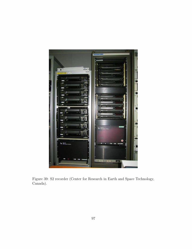
Figure 39: S2 recorder (Center for Research in Earth and Space Technology,Canada).

97

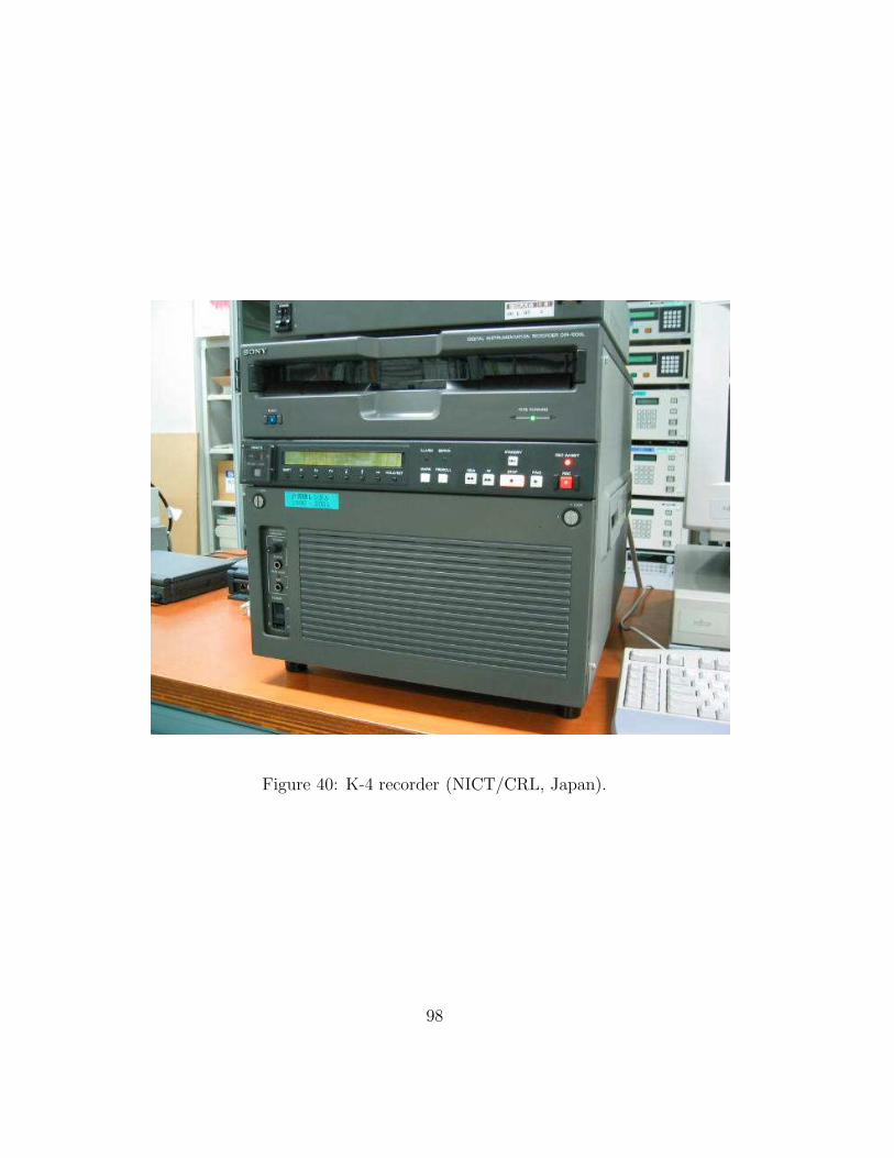
Figure 40: K-4 recorder (NICT/CRL, Japan).

98

Figure 41: Automated tape handler for K-4 (NICT/CRL, Japan).

99

Figure 42: Magnetic tapes used in VLBI: S2 (top left), K-4 (left), andVLBA/Mark IV (right).

100

2 Overview of the VLBI System

2.1 MK–3 As a Prototype of Modern VLBI Systems

Figure 43 shows a schematic view of the Mark III / K-3 VLBI system, oftencalled “MK–3”, which was initially developed by the MIT Haystack Obser-vatory with sponsorship from NASA, and by the CRL (now NICT), in thelate 1970’s. Although this system has now been almost replaced by newersystems, such as the Mark IV, Mark V, VLBA, K-4, K-5 and VSOP, manyimportant elements of these modern VLBI systems were implemented for thefirst time in the MK–3 system, and have been further developed in the latestsystems. Therefore, we briefly describe here the basic components, and theirfunctions, of the MK–3 system.

S and X LowNoise Amplifiers

Video Converter

Formatter


Data Recorder

Local Oscillator

P & D Ground Unit


P & D Antenna Unit

ControlComputer

AntennaControl Unit

Downconverter

VLBI Terminal

Control Building

Receiver RoomS X

Figure 43: A schematic view of the Mark III / K-3 VLBI system.

The MK–3 system was originally developed mainly for realizing high–

101

precision VLBI geodesy, although the system has been extensively used forastrophysical radio source imaging observations as well. In order to accu-rately estimate the group delay, the system adopted a multi–frequency chan-nel design, together with high–speed recording technology; these featureshave been retained in most of the latest systems.

2.1.1 Dual–Frequency Reception

In geodetic applications, a VLBI antenna receives radio waves from distantextragalactic sources usually at two frequencies simultaneously, in order tocorrect the effects of frequency–dependent propagation delay in the iono-sphere. The two frequencies, S–band (2 GHz) and X–band (8 GHz), aremost widely used in global geodetic VLBI observations. The RF frequencybands in the MK–3 system typically covered 200 MHz for S–band (e.g., from2120 to 2320 MHz), and 420 MHz for X–band (e.g., from 8180 to 8600 MHz).Multi–frequency coaxial feed horns are widely used for dual–frequency recep-tion. Other systems, including FSS (Frequency Selective Surfaces) and spiralarrays (see, e.g., Figure 44), are also used.

Figure 44: S/X spiral–array feed system, developed by Hosei University,Japan, is used for dual–frequency reception in VERA.

2.1.2 First Frequency Conversion

In the receiver room, usually built in the antenna structure, the RF signalsare amplified by the S–band and X–band low–noise amplifiers, and down-

102

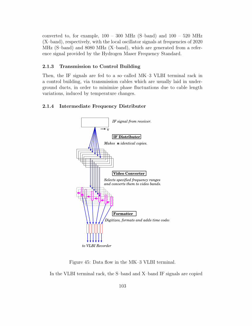
converted to, for example, 100 – 300 MHz (S–band) and 100 – 520 MHz(X–band), respectively, with the local oscillator signals at frequencies of 2020MHz (S–band) and 8080 MHz (X–band), which are generated from a refer-ence signal provided by the Hydrogen Maser Frequency Standard.

2.1.3 Transmission to Control Building

Then, the IF signals are fed to a so–called MK–3 VLBI terminal rack ina control building, via transmission cables which are usually laid in under-ground ducts, in order to minimize phase fluctuations due to cable lengthvariations, induced by temperature changes.

2.1.4 Intermediate Frequency Distributer

ν

Makes n identical copies.

Selects specified frequency rangesand converts them to video bands.

IF signal from receiver.

IF Distributer

Video Converter

Digitizes, formats and adds time codes.

to VLBI Recorder

Formatter

Figure 45: Data flow in the MK–3 VLBI terminal.

In the VLBI terminal rack, the S–band and X–band IF signals are copied

103

over to 6 (S–band) and 8 (X–band) identical signals, respectively, by theso–called “Intermediate Frequency Distributer” unit (Figure 45).

2.1.5 Baseband Conversion

The 6 and 8 identical IF signals are then sent to 14 special units consisting offrequency downconverters, called “Video Converters” (VC’s) (or “BasebandConverters”, BBC’s) located in the same rack. Each Video Converter selectsa specified frequency range in the IF band, and downconverts this range intoa video band, typically from 0 to 2 MHz. For this purpose, a frequency syn-thesizer, which is built in the Video Converter, generates an LO frequencyat the edge of the selected IF range, using a reference signal provided by theHydrogen Maser Frequency Standard. The Video Converter is equipped witha sideband–rejection mixer, which is capable of converting both lower andupper sidebands around the selected LO frequency, separately. Thus, in totalup to 28 (14 × 2 SB’s) baseband frequency channels are generated by the14 Video Converters. Usually, of course, the baseband channels are selectedin such a way that they correspond to different RF frequency ranges. Table6 and Figure 46 show an example of the LO frequency distribution used ina recent geodetic VLBI observation. This apparently strange distribution ofthe data among the baseband channels, which are to be subsequently digi-tized and recorded, are spread over fairly wide ranges of the RF bands; Thisis specifically designed for better estimation of the group delay observablesvia a technique called “bandwidth synthesis”, which will be discussed later.

8200 8250 8300 8350 8400 8450 8500 8550 8600RF frequency (MHz)

2220 2240 2260 2280 2300 2320 2340 2360RF frequency (MHz)

Figure 46: Distributions of baseband channels within the RF frequencyranges, in a sample geodetic VLBI observation, as used in Table 6. Top:X–band, and bottom: S–band.

104

Ch# band LO freequency (MHz) bandwidth (MHz)

1 X 8209.99 4.00

2 X 8219.99 4.00

3 X 8249.99 4.00

4 X 8309.99 4.00

5 X 8419.99 4.00

6 X 8499.99 4.00

7 X 8549.99 4.00

8 X 8569.99 4.00

9 S 2239.99 4.00

10 S 2244.99 4.00

11 S 2259.99 4.00

12 S 2289.99 4.00

13 S 2319.99 4.00

14 S 2329.99 4.00

15 S 2344.99 4.00

16 S 2354.99 4.00

Table 6: An example of the distribution of LO frequencies in baseband chan-nels. Note that this example is taken from a recent geodetic VLBI observa-tion, which uses the K-4 VLBI system. The K-4 is newer than the MK–3,and has 16 Video Converters (therefore, 16 baseband channels), each with 4MHz bandwidth.

105

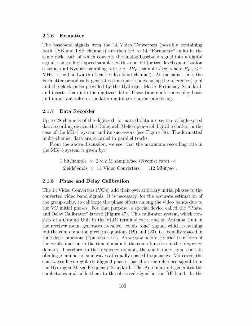
2.1.6 Formatter

The baseband signals from the 14 Video Converters (possibly containingboth USB and LSB channels) are then fed to 14 “Formatter” units in thesame rack, each of which converts the analog baseband signal into a digitalsignal, using a high–speed sampler, with a one–bit (or two–level) quantizationscheme, and Nyquist sampling rate (i.e. 2BV C samples/sec, where BV C ≤ 2MHz is the bandwidth of each video band channel). At the same time, theFormatter periodically generates time mark codes, using the reference signaland the clock pulse provided by the Hydrogen Maser Frequency Standard,and inserts them into the digitized data. These time mark codes play basicand important roles in the later digital correlation processing.

2.1.7 Data Recorder

Up to 28 channels of the digitized, formatted data are sent to a high–speeddata recording device, the Honeywell M–96 open–reel digital recorder, in thecase of the MK–3 system and its successors (see Figure 38). The formattedmulti–channel data are recorded in parallel tracks.

From the above discussion, we see, that the maximum recording rate inthe MK–3 system is given by:

1 bit/sample × 2 × 2 M sample/sec (Nyquist rate) ×2 sidebands × 14 Video Converters = 112 Mbit/sec.

2.1.8 Phase and Delay Calibration

The 14 Video Converters (VC’s) add their own arbitrary initial phases to theconverted video band signals. It is necessary, for the accurate estimation ofthe group delay, to calibrate the phase offsets among the video bands due tothe VC initial phases. For that purpose, a special device called the “Phaseand Delay Calibrator” is used (Figure 47). This calibrator system, which con-sists of a Ground Unit in the VLBI terminal rack, and an Antenna Unit inthe receiver room, generates so-called “comb–tone” signal, which is nothingbut the comb function given in equations (19) and (23), i.e. equally spaced intime delta functions (“pulse series”). As we saw before, Fourier transform ofthe comb function in the time domain is the comb function in the frequencydomain. Therefore, in the frequency domain, the comb–tone signal consistsof a large number of sine waves at equally spaced frequencies. Moreover, thesine waves have regularly aligned phases, based on the reference signal fromthe Hydrogen Maser Frequency Standard. The Antenna unit generates thecomb–tones and adds them to the observed signal in the RF band. In the

106

actual observations, the LO frequencies of the Video Converters are selectedin such a way that at least one comb–tone signal falls into each of the videobands (e.g., at a frequency of 10 kHz in the MK–3 system). The comb–tonesignals pass through the same units as the observed data do, and, therefore,are affected by the same phase offsets due to the VC initial phases, as theobserved data are. Then, the data containing the comb–tones are digitizedand recorded. These comb–tones are later detected in the correlation pro-cessing, and the phases of the comb–tones in the different video bands arecompared with each other, in order to estimate, and then remove from theobserved data, the unknown phase offsets due to the VC initial phases.

Formatter


Data Recorder

Ground Unit

Antenna Unit

H-MaserFrequencyStandard

A cos (ωt)

A cos [ω(t-τ)] Σ Bn cos [nω(t-τ)]n

Round-tripmeasurement of cable delay τ

Antenna feed

t

ω

Fourier transform

Comb pulses in time

Comb tones in spectrum

Video Converter

Comb tones go throughthe same path as theradio source signal.

Comb tones at 10 kHz ofevery video band channel

ω10 kHz

Correlation Processor

tPhase of the 10 kHz tone is detected bycorrelating with a standard 10 kHz signal.

Figure 47: Phase and delay calibration system in the MK–3.

107

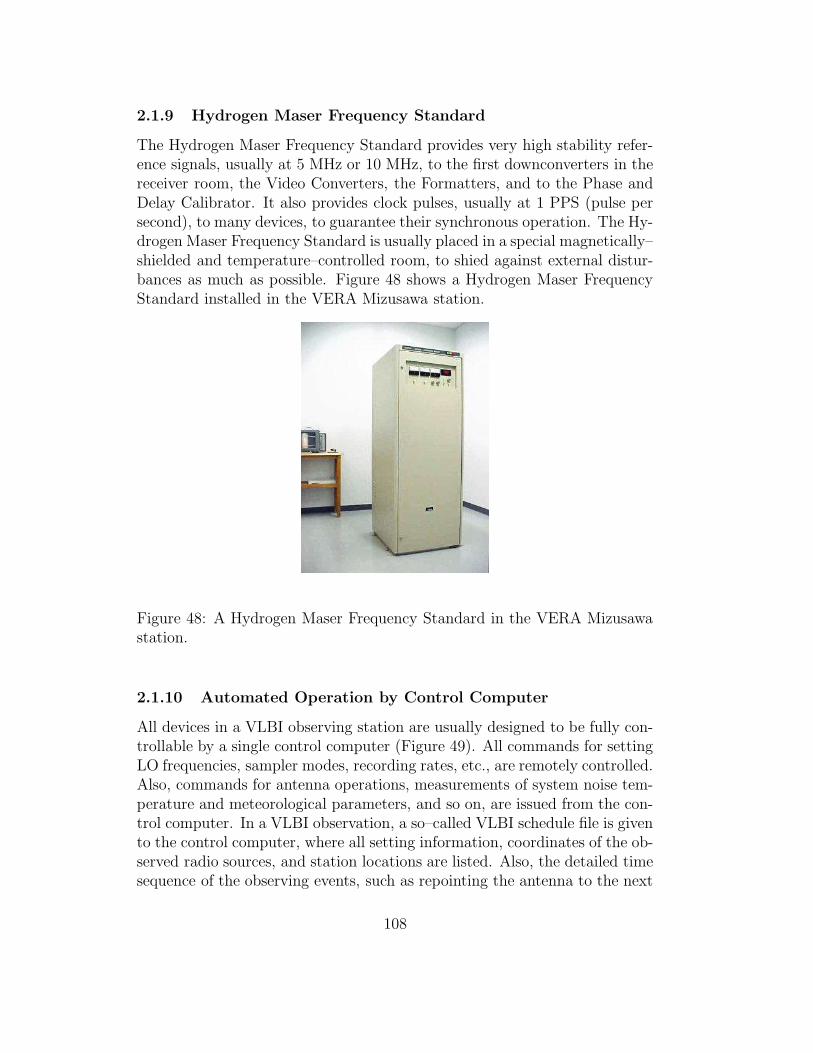
2.1.9 Hydrogen Maser Frequency Standard

The Hydrogen Maser Frequency Standard provides very high stability refer-ence signals, usually at 5 MHz or 10 MHz, to the first downconverters in thereceiver room, the Video Converters, the Formatters, and to the Phase andDelay Calibrator. It also provides clock pulses, usually at 1 PPS (pulse persecond), to many devices, to guarantee their synchronous operation. The Hy-drogen Maser Frequency Standard is usually placed in a special magnetically–shielded and temperature–controlled room, to shied against external distur-bances as much as possible. Figure 48 shows a Hydrogen Maser FrequencyStandard installed in the VERA Mizusawa station.

Figure 48: A Hydrogen Maser Frequency Standard in the VERA Mizusawastation.

2.1.10 Automated Operation by Control Computer

All devices in a VLBI observing station are usually designed to be fully con-trollable by a single control computer (Figure 49). All commands for settingLO frequencies, sampler modes, recording rates, etc., are remotely controlled.Also, commands for antenna operations, measurements of system noise tem-perature and meteorological parameters, and so on, are issued from the con-trol computer. In a VLBI observation, a so–called VLBI schedule file is givento the control computer, where all setting information, coordinates of the ob-served radio sources, and station locations are listed. Also, the detailed timesequence of the observing events, such as repointing the antenna to the next

108

source, tape start, tape stop, and so on, are given in Universal Times (UT).

S and X LowNoise Amplifiers

Video Converter

Formatter


Data Recorder

Local Oscillator

P & D Ground Unit


P & D Antenna Unit

ControlComputer

AntennaControl Unit

Downconverter

VLBI Terminal

Control Building

Receiver RoomS X

Schedule File

Field System

LogFile Mark III

DB

Observation sequenceSource informationAntenna information

Figure 49: A typical automated VLBI operation system.

The control computer automatically conducts all steps of the observationby issuing commands to the antenna control unit, VLBI terminal, and datarecorder, according to the schedule file. As a result, the only remaining task,to be done by an operator in a normal VLBI observation, is to change therecording tapes once an hour or, at most a few times a day, depending on thesystem design. The most widely used software for automated control of theVLBI equipment, which was developed in the NASA Goddard Space FlightCenter (NASA/GSFC), is called the “VLBI Field System”.

2.2 Modern VLBI Systems

2.2.1 New Recording and Fiber–Link Systems

The major successors of the MK–3 system are listed in Figure 37. They arethe VLBA and Mark IV sytems based on the advanced head controls of the

109

Honeywell M–96 recorder (Figure 38), the S2 system using 8 video cassetterecorders in parallel (Figure 39), and the K-4 system based on an ID1 digitalvideo cassette recorder (Figure 40).

Nowadays, modern VLBI recording systems with 1 Gbps recording speedhave been developed and some of them are already in use (Table 7). Theyare the Mark V system (Figure 50) using a hard disk array instead of themagnetic tapes, the K–5 system also based on the hard disk array (Figure51), the GBR-1000 system based on an HDTV video cassette recorder (Figure52), the VERA recording system based on a new ID1 digital video cassetterecorder (Figure 53), and the fiber–linked e–VLBI.

name type bitrate

Mark V hard disk array 1024 Mbps

K–5 hard disk array 512 & 2048 Mbps

GBR-1000 HDTV 1024 Mbps

VERA ID1 1024 Mbps

e–VLBI real–time fiber link > 2048 Mbps

Table 7: New generation recording and fiber–link systems.

Figure 50: Mark V recording system based on a new hard disk array design.

110

Figure 51: K–5 VLBI terminal.

111

Figure 52: GBR-1000 1 Gbps VLBI system based on an HDTV video cassetterecorder.

112

Figure 53: VERA recording system based on a new ID1 digital video cassetterecorder.

2.2.2 Digital Baseband Converters

Another progress is beeing made in several countries for implementing digitalBBC systems based on the digital filtering technology. The idea is first to

Figure 54: Data Aquisition System of the KVN adopting the digital filtersystem for the baseband conversion.

digitize a wideband IF data using a high–speed sampler (analog–to–digitalconverter), and second to cut the digital data into baseband channels bymeans of a high–speed digital filter. Then the baseband data will no longersuffer from irregular bandpass characteristics of analog BBC’s and arbitrary

113

phases added by the LO’s of the BBC’s. In fact, the digital filter can in prin-ciple remove the phase calibration systems discussed above, as far as the LOphase problem only is concerned. Also, the digital filter allows flexible orga-nization of baseband channels meeting different scientific requirements. Forexample, a single channel ultra–wideband data could be suited to imagingvery weak continuum sources, while 16 channel data are necessary for geode-tic observations. Such a digital BBC system was developed and successfullyutilized in 4 stations of the VERA array.

Figure 54 shows the Data Aqusition System (DAS) of the KVN whichuses a digital BBC system for the baseband conversion. The DAS systemincludes 4 high–speed samplers located in the receiver room. The 4 samplersare equipped for 4 frequency bands to be simultaneously received for mm–wave VLBI observations. Each sampler is capable of digitizing IF data of512 MHz bandwidth using the higher–order sampling technique discussedearlier with 1 Gsps speed in the 2–bit quantization mode (therefore, theoutput bit–rate is 2 Gbps). The digital data are transmitted to the controlbuilding via optical fiber cables. Then the digital filter forms 1, 2, 4, 8, and16 baseband channels with bandwidths of 256, 128, 64, 32, and 16 or 8 MHz,correspondingly, out of the 512 MHz / 2–bit / 1 Gsps input, depending onscientific purposes.

2.2.3 e–VLBI

Several groups in the world are now developing VLBI systems based on high–speed data transmission techniques via optical fibers. The idea is to replacethe data tapes by ultra–wide–band transmission cables. This technologyis now called “e–VLBI”. Figures 55 and 56 show the first successful EVN(European VLBI Network) e–VLBI observation conducted by three observa-tories, in April 2004, and a beautiful image of the gravitational lens objectB0218+357 obtained through this coordinated effort.

Of course, this technology by no means transforms VLBI into a connected–element interferometer, since the frequency standards in different stationsmust remain independent, in view of the essential technical difficulties totransmit reference signals over thousands of kilometers without significantdelays or phase fluctuations. Nevertheless, this technology will bring VLBImuch closer to the connected–element interferometer, in the sense that theobserved data could be correlated and analyzed in real–time, or almost inreal time (“near–real-time”). For example, pioneering real–time e–VLBI ex-periments conducted in the KSP (Key Stone Project, 1995–2001) of the CRL(now NICT) regularly yielded final geodetic results a few minutes after eachobservation. Moreover, the optical fiber cables offer even higher data trans-

114

Figure 55: First EVN e–VLBI observation (2004 April) using radio telescopesat Jodrell Bank, UK; Westerbork, the Netherlands; and Onsala, Sweden. Thelower panels show beats of the fringe amplitudes produced by two closelyspaced sources, and an image map obtained during the observation (fromURL: http://www.jive.nl).

Figure 56: A close–up view of the image of a radio–loud gravitational lensJVAS B0218+357, obtained in the first EVN e–VLBI observation (from URL:http://www.jive.nl).

115

mission rates, and therefore higher sensitivity, than the magnetic tapes, orhard disk arrays. Real–time VLBI experiments with 2.5 Gbps transmissionrate have been successfully conducted since 1998 (Figure 57). Even muchhigher transmission rates are expected in new connected–element interfer-ometer arrays (for example, 96 Gbps / antenna is planned for the ExpandedVLA (EVLA), and for the Atacama Large Millimeter and submillimeter Ar-ray (ALMA)). High–speed correlators are now being developed to meet thesehigh data rates.

At the same time, less expensive and more widely accessible VLBI datatransmission, via broad–band Internet using the IP protocol, is also beingintensively studied, and has been successfully tested. This IP–based e–VLBI,or IP–VLBI, seems to be a particularly promising technology which willmake VLBI observations much more user–friendly for many astronomers andgeophysicists around the world. The K–5 system, developed at the NICT, isdesigned to realize the IP–VLBI concept (Figure 58).

2.2.4 VLBI Standard Interface (VSI)

Another remarkable example of progress in modern VLBI is the definition ofthe international “VLBI Standard Interface (VSI)” specifications(http://web.haystack.edu/vsi).

The world VLBI community has long suffered from incompatibily of thevarious different VLBI systems, shown above, which had been developed indifferent institutions. In order to cross–correlate data recorded on differenttapes by different VLBI systems A and B, say, one had to convert the formatof B’s data into A’s format, copy the converted data to A’s tape, and thencross–correlate them with A’s correlator, or vice versa.

The purpose of the VSI specifications is to make all VLBI systems in theworld compatible, provided only that they obey these standard specifications.

So far, a hardware specification called “VSI–H”, and a software specifica-tion called “VSI–S”, were worked out by an international working group ofVLBI specialists. Another specification for e–VLBI, to be called “VSI–E”,is now under intensive discussion and development.

The VSI–H hardware specification defines a standard interface betweenthe “data–acquisition system (DAS)” (i.e. VLBI terminals) and the “data–transmission sytem (DTS)” (i.e. tapes or hard disks), as well as between the“data–transmission system” and the “data–processing system (DPS)” (i.e.correlators). Figure 59 shows how the interface could be realized. EveryDAS, DTS, and DPS must have common connectors with well specified pin–assignments and data rates. The actual data transmission media (the handlerunits for tapes or hard–disks) are supposed to be equipped with a “data

116

Figure 57: 2.5 Gbps fiber–linked real–time VLBI experiment “OLIVE–GALAXY”, Japan (1998, December).

117

Figure 58: IP–based e–VLBI developed for the K–5 system.

118

Figure 59: VSI-H functional diagram (http://web.haystack.edu/vsi).

119

input module (DIM)”, and a “data output module (DOM)”, which interfacethe common connectors, and the connectors of the handler hardware. Theactual data formats in the individual data transmission media are arbitrary,provided that the DIM accepts the input data stream (specified by VSI-H),and the DOM yields the output data stream (also specified by VSI-H).

The VSI–S software specification defines protocols for handling VSI–H–compliant equipment.

A number of VSI–H–compliant VLBI systems have been developed invarious countries, and successfully cross–correlated with each other.

3 Difficulties in Ground–Based VLBI

UNFINISHED.

4 Correlation Processing in VLBI

UNFINISHED.

5 Observables of VLBI

UNFINISHED.

120

References

Allan, D.W., 1966, Statistics of Atomic Frequency Standards,Proc. IEEE, 54, 221–230.

Hagen, J.B., and Farley, D.T., 1973, Digital Correlation Tech-niques in Radio Science, Radio Sci., 8, 775–784.

Iguchi, S., and Kawaguchi, N., 2002, Higher–Order Sampling,Over Sampling and Digital Filtering Techniques for Radio In-terferometry, IEICE, Trans. Commun., E85-B, 1806–1816.

Meijering, E., 2002, A Chronology of Interpolation: From AncientAstronomy to Modern Signal and Image Processing, Proc,IEEE, 90, 319–342.

Papoulis, A., 1984, Probability, Random Variables, and Stochas-tic Processes, 2nd Edition, McGraw-Hill (New York).

Price, R., 1958, A Useful Theorem for Nonlinear Devices HavingGaussian Inputs, IRE Trans. Inf. Theory, IT-4, 69–72.

Rogers, A.E.E., and Moran, J.M., 1981, Coherence Limits forVery–Long–Baseline Interferometry, IEEE Trans. Instrum.Meas., IM–30, 283–286.

Shannon, C.E., 1949, Communication in the Presence of Noise,Proc. IEEE, 37, 10–21.

Thompson, A.R., Moran, J.M., and Swenson, G.W., Jr., 2001,Interferometry and Synthesis in Radio Astronomy, John Wiley& Sons (New York).

Takahashi, F., Kondo, T., Takahashi, Y., and Koyama, Y., 2000,Very Long Baseline Interferometer, Ohmsha (Tokyo).

Van Vleck, J.H., and Middelton, D., 1966, The Spectrum ofClipped Noise, Proc. IEEE, 54, 2–19.

121

very long baseline interferometry - yamaguchi...

Documents