phylogenetics2

Phylogenetics Workshop

Part II : Model-based tree building

De Landtsheer Sébastien, University of Luxemburg

Ahead of the BeNeLux Bioinformatics Conference 2011

Outline of the Workshop

Part I :• General introduction• Alignments• Distance-based methods

Part II :• Maximum likelihood trees• Bayesian trees

Part III :• Advanced bayesian phylogenetics• Hypothesis testing

Outline of the Workshop

Programs featured :

- Topali (http://www.topali.org/download.shtml)- ModelTest in Java GUI

(http://darwin.uvigo.es/software/jmodeltest.html)- BEAUti, BEAST and Tracer

(http://beast.bio.ed.ac.uk/Main_Page)

-

Model-based tree building

Reminder : the main problem in phylogenetics is the HUGE number of possible trees to choose from

What makes a good tree ?

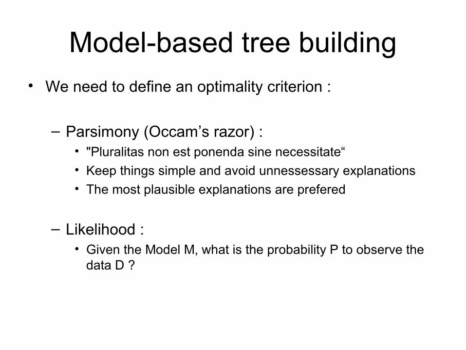
Model-based tree building• We need to define an optimality criterion :

– Parsimony (Occam’s razor) :• "Pluralitas non est ponenda sine necessitate“• Keep things simple and avoid unnessessary explanations• The most plausible explanations are prefered

– Likelihood :• Given the Model M, what is the probability P to observe the

data D ?

Parsimony

Parsimony• What tree represents the minimal number of changes

along the phylogeny ?

• Natural way to find the most plausible (less expensive) explanation

• Example 1 :

ATGTAACGTA

ATGTCAGGTA

ATGTCACGTT

ParsimonyPossible tree 1 :

ACA

CCA

CCT CGA

ACT

4 changes

C->A

T->A

C->A

C->G

ParsimonyPossible tree 2 :

ACA

ACA

AGA ACT

CGA

3 changes

A->C

G->C

No change

A->T

ParsimonyParsimony methods will search for the most parsimonious tree using a simple scoring system. Two are commonly used :

- equal : 0 1 1 1 - tv4 : 0 4 1 4

1 0 1 1 4 0 4 1

1 1 0 1 1 4 0 4

1 1 1 0 4 1 4 0

ParsimonyHow to search the tree space ?

- Brute force : trying all possible trees. Possible up to ~ 11 taxa on modern computers

- Heuristic search : trying arrangements of the (so far) best tree by making tiny changes. If the new tree is better it becomes the (so far) best tree. If not it is rejected and another rearrangement is tried

Tree rearrangements

• Nearest-Neighbor Interchange (NNI)

Tree rearrangements

• Subtree Pruning and Regrafting (SPR)

Tree rearrangements

• Tree Bisection and Reconnection (TBR)

Likelihood

• Probability to observe the data under the model

– Data : already collected, won’t change, holy material

– Model : idea about how things happened, with which we can do whatever we want :

– Tree topology + branch lengths = « the tree »– Mechanism of sequence evolution = « the model » :

- nucleotide composition

- substitution matrix

Likelihood

• The coin-flipping analogy :

– Experimental setting : flipping a coin once

– Data : heads

– Model 1 : fair coin; Likelihood = 0.5

– Model 2 : 2-headed coin; Likelihood = 1

Likelihood

• The coin-flipping analogy :

– Experimental setting : flipping a coin 10 times

– Data : h=6, t=4

– Model 1 : fair coin; Likelihood = 0.205

– Model 2 : 2-headed coin; Likelihood = 0

– Model 3 : unfair coin with p=0.6; Likelihood = 0.251

Likelihood

• Likelihood with DNA :

– Let’s assume a nucleotide composition of :

• A : 25%

• C : 25%

• G : 25%

• T : 25%

– What is the likelihood of the sequence « A » ?

– What is the likelihood of the sequence « ATGTAACA »?

Likelihood



• A : 25%

• C : 25%

• G : 25%

• T : 25%


25%

– What is the likelihood of the sequence « ATGTAACA » ?

25%^8 = 0.00001526

Likelihood



• A : 50%

• C : 10%

• G : 10%

• T : 30%



Likelihood



• A : 50%

• C : 10%

• G : 10%

• T : 30%


50%


50%^4 * 10% * 10% * 30%^2 = 0.0001875

Likelihood


– Under any model, the sum of the likelihoods of all nucleotides, or all dinucleotides, or all possible data is 1 :

• Let’s A=0.1; C=0.4; G=0.2; T=0.3 • => L(A)+ L(C)+ L(G)+ L(T)=1

=> L(AA)+ L(AC)+ L(AG)+ L(AT)+ L(CA)+ L(CC)+ L(CG)+ L(CT)+ L(GA)+ L(GC)+ L(GG)+ L(GT)+ L(TA)+ L(TC)+ L(TG)+ L(TT)=1

=> The probability that some data exist is 1 (and that’s reassuring)

Likelihood


– Nucleotide composition model :

A=0.1; C=0.4; G=0.2; T=0.3

– Nucleotide substitution model : A C G T

A 0.976 0.01 0.007 0.007

C 0.002 0.983 0.005 0.01

G 0.003 0.01 0.979 0.007

T 0.002 0.013 0.005 0.979

– Tree model : one branch

– Data : « A » and « C »

Likelihood


A C

Likelihood of « A » = 0.1

Likelihood of a change from A to C = 0.01

Likelihood of our Data given the Model = 0.1 * 0.01 =

0.001

Likelihood

• Let’s try with a more complicated alignment :

CCAT CCGT

Likelihood of our Data given the Model =

0.4 * 0.983 * 0.4 * 0.983 * 0.1 * 0.007 * 0.3 * 0.979 =

0.0000300

But this is for a branch length of arbitrary unit 1

Likelihood

• We can get the probabilities for longer branches by multiplying the matrix by itself :

0.976 0.01 0.007 0.007

0.002 0.983 0.005 0.01

0.003 0.01 0.979 0.007 =

0.002 0.013 0.005 0.979

0.953 0.02 0.013 0.015

0.005 0.966 0.01 0.02

0.007 0.02 0.959 0.015

0.005 0.026 0.01 0.959

2

Likelihood

• We can calculate the likelihood of D given M under different branch lengths :

Branch length likelihood

1 0.0000300

2 0.0000559

3 0.0000782

10 0.000162

15 0.000177

20 0.000175

30 0.000152

Likelihood

• We can calculate the likelihood of D given M under different branch lengths :

Likelihood

• What do the program do ?– Programs : PAUP, PAML, IQPNNI

– General scheme :• Generate a tree (Neighbor-joining)• Calculate its likelihood

• Optimizing branch lengths• Perform a tree rearrangement (NNI, SPR, TBR)• Evaluate the new tree

– No garantee to find the single best tree, but usually finds a nearly-optimal one

Bayesian Trees

• Are we happy with one tree ?

– Since we cannot test all trees to find the best, we need to find a nearly-optimal one, but how good is a nearly optimum ?

– We would like to find a collection of reasonably good trees and evaluate these

– Probabilistic view : what is the probability of the Data given the Model

– Bayesian view : given the Data, what is the probability of the Model ?

0

0.05

0.1

0.15

0.2

0.25

0.3

1 2 3 4 5 6 7 8 9 10

Bayesian Trees

• Exemple : red and black balls in an urn

We know p=0.5

What is the chance to take exactly 4 black and 6 red ?

We can solve with a binomial distribution

P(D given M) = 20.5%

Bayesian Trees

• Exemple : red and black balls in an urn

We do not know p

We actually take exactly 4 black and 6 red

What is p ? With what confidence ?

We take 10 more balls. They are all black. How does the new information changes our estimate ?

?

Bayesian Trees

• Bayesian phylogenetics : the prior

– We need a prior assumption, which can be strong or not. They represent our A PRIORI HYPOTHESIS ABOUT THE PHENOMENON. They need to be formulated as a prior distribution of the possible values of the parameters

– Our inference will depend both of the prior and the data. The more data we possess, the less the final result will depend of the prior

Bayesian Trees

• Bayesian phylogenetics : example priors– 1) « I have no idea whatsoever what the proportion of the red and black

balls could be »

0

0.005

0.01

0.015

0.02

0.025

0 0.1 0.2 0.3 0.4 0.5 0.6 0.7 0.8 0.9 1

Bayesian Trees

• Bayesian phylogenetics : example priors– 2) « I am nearly sure the proportion of red and black balls is 0.5 »

0

0.01

0.02

0.03

0.04

0.05

0.06

0.07

0.08

0 0.1 0.2 0.3 0.4 0.5 0.6 0.7 0.8 0.9 1

Bayesian Trees

• Bayesian phylogenetics : example priors– 3) « I know the balls is the urn are sampled from a big population of

balls, and this global population has a p of 0.5 »

0

0.005

0.01

0.015

0.02

0.025

0.03

0.035

0.04

0.045

0 0.1 0.2 0.3 0.4 0.5 0.6 0.7 0.8 0.9 1

Bayesian Trees

• Bayesian phylogenetics : example priors– 4) « I know the proportion of balls is around 0.82, and deviations are

more likely to be in high values than low ones. I also know that values below 0.5 are impossible for some reason »

0

0.01

0.02

0.03

0.04

0.05

0.06

0 0.1 0.2 0.3 0.4 0.5 0.6 0.7 0.8 0.9 1

Bayesian Trees

• Bayesian phylogenetics : the posterior

– We get as a result a posterior distribution of the possible values of p

– From this distribution (probability density function) we can directly know the confidence we have in our estimate, estimated as Highest Probability Density (95%HPD)

=> We do not need to subsample (bootstrap) We can directly see the uncertainty in the data

Bayesian Trees

• Bayesian phylogenetics : example posteriors– 1) « I know the balls is the urn are sampled from a big population of

balls, and this global population has a p of 0.5 ». Data = 6 blacks, 4 reds (orange) or 60 blacks, 40 reds (purple)

0

0.02

0.04

0.06

0.08

0.1

0.12

0.14

0.16

0.18

0 0.1 0.2 0.3 0.4 0.5 0.6 0.7 0.8 0.9 1

Data

Prior

0

0.01

0.02

0.03

0.04

0.05

0.06

0.07

0.08

0 0.1 0.2 0.3 0.4 0.5 0.6 0.7 0.8 0.9 1

Bayesian Trees

• Bayesian phylogenetics : example posteriors– 2) « I am nearly sure the proportion of red and black balls is 0.5 ». Data

= 6 blacks, 4 reds (orange) or 60 blacks, 40 reds (purple)

Data

Prior

0

0.1

0.2

0.3

0.4

0.5

0.6

0.7

0.8

0.9

1

1 2 3

p

Bayesian Trees

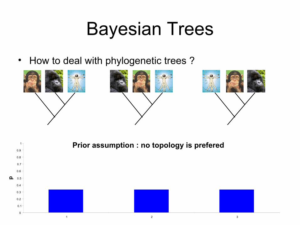
• How to deal with phylogenetic trees ?

Prior assumption : no topology is prefered

Bayesian Trees

• After analysis of the data

0

0.1

0.2

0.3

0.4

0.5

0.6

0.7

0.8

0.9

1

1 2 3

p

Posterior : one of the topologies is prefered

Bayesian Trees

• Markov Chains : how to find the top of the mountain if you are blind ? (the Metropolis-Hastings algorithm)

– MC are algorithms that will start at some arbitrary point in the parameter space and make a small random step

– The step is accepted with a high probability if it increases the posterior probability, low otherwise

– If the step is rejected, the chain returns to its previous state and tries a new random move

Bayesian Trees

• Markov Chains : how to find the top of the mountain if you are blind ?

New altitude is higher : accept always

New altitude is higher : accept rarely

Bayesian Trees

• Markov Chains : how to avoid getting stuck in local maxima ? (Metropolis Coupling)

=> Run multiple « heated » chains and jump from one to another

Bayesian Trees

• Markov Chains : how to get the posterior distribution (Monte-Carlo sampling)

Bayesian Trees

• MCMCMC : what makes a good run ? (a hairy caterpillar)

– No trend in the stable state (convergence)• Sufficient run time

• Good data

– Good mixing in order to have a good sample from the posterior (adequecy of the steps)

• If steps too close to the current states : always accepted• If steps to different : too often rejected• Best mixing is at intermediate values

Bayesian Trees


– 1) Steps too small

Bayesian Trees


– 2) Steps too big

Bayesian Trees


– 3) Steps of acceptable length

Bayesian Trees


Bayesian Trees

• How to set up a bayesian phylogenetic analysis ?

2 main programs :

• MrBayes : command-line

• BEAST : User interface

Molecular Clocks

Global clock No clock

Local clock Relaxed clock

BEASTINGFlexible package :

- BEAUti : to make the xml files

- BEAST : actual calculations

Metropolis – Hastings MCMC sampling

- Tracer : to analyse results

- TreeAnnotator : to sum trees

BEASTINGBEAUti :

Allows dated tips via the Guess dates function

A priori sub-taxa

Setting a model :

- Substitution model (HKY, GTR, TN93)- Site heterogeneity (gamma distribution)- codon partition : (1, 2, 3) (1+2, 3) or none- codon position independence : model parameters and/or rates- Molecular clock : from strict to uncorrelated relaxed

BEASTINGSetting the model priors :

Difficult task, try several approaches, usually the default are good enoughIf the data is good, the priors do not matter…

Setting the operators and the tuning parameters :

Determines the « moves » made by the chain→ auto-optimize function

MCMC settings : - chain lenght 10 000 000, sampling 1000 is a good default - anyway we want about 10 000 points

BEASTINGTracer : result analysis

1) chain convergence diagnosticBad convergence

BEASTINGTracer : result analysis

1) chain convergence diagnosticGood convergence

Sampling from the converged chain provides the posterior distribution of the parameters

BEASTINGAuto-correlation time (ACT) measures independency of sampling procedure

Effective sample size (ESS) = chain length/ACT

Rule of thumb : ESS < 100 is very badESS > 200 is good

Both chain convergence and ESS have to be checked for each parameter

Depending the problem : - increase chain length and decrease sampling frequency- increase burn-in- question models, alignment, priors, tuning

BEASTINGCombining runs :

- different runs with the same xml file- longer runs, different burn-in or sampling- different priors given to the parameters- different operators- LogCombiner even allows resampling from the chain

It does not make sense to combine runs from differents data sets or (even slightly) different models

BEASTINGTreeAnnotator output :

Model Selection

Model Selection : LRTs

Likelihood Ratio Tests are a standard way to compare the fit of two models :

LRT = 2 (logL1 – logL0)

When the models are nested, this statistic is approximately distributed as a χ2 distribution

- only for nested models (H0 is a special case of H1)

- d.f = difference of parameters numbers in the 2 models

- advantage : statistaically sound

- disadvantage : the χ2 distribution only holds for enough data

Model Selection : AIC

Akaike information criterion is another goodness-of-fit measure

AIC = 2k – 2 logL(Data, Model)

where k is the number of parameters in the model

- valid for non-nested models

- sort of likelihood that would be « penalized » if using too many parameters

- more criteria exists (AICc, BIC, etc…)

Bayes FactorsBF = Marginal Likelihood Model1 / Marginal Likelihood Model 2 = log-L1 – log-L2

In practice, the marginal likelihoods are difficult to compute, but are approximated by taking the harmonic mean of the log-likelihoods (might be better in later versions of BEAST)

Rule of thumb : BF < 3 : no significant improvement with model 1 compared with model 2 3 < BF < 10 : significant improvement with model 1 BF > 10 : decisive improvement with model 1

Big advantage of Bayes Factors compared to LRTs : direct comparison of two non-nested models

Model Selection : Topali


Click « Run » : runs remotely

CTRL-click « Run » : runs locally

Model Selection

BEASTing : MCMC robothttp://hydrodictyon.eeb.uconn.edu/people/plewis/software.php

BEASTing

Model Selection

Model Selection

10 000 samples

BEASTing

Beasting

Beasting

.fst

BEAUti

.beast (.xml)

.log .trees

Tracer TreeAnnotator

Parameters of interest Tree

Beasting

Beasting : practicalsThe file « FPV.fas » contains an alignment of 7 feline papilloma virus sequences. Our goal is to

determine the rate of evolution of each lineage based on the divergence dates of their host species. We have some estimates of the speciation times from the littérature.

The file « RSVA.fas » contains an alignment of 35 human respiratory synctitial virus, group A. Our goal is to estimate the rate of evolution, the date of the most recent ancestor, and to get a good tree with measures of statistical support.

The file « Flu.fas » contains an alignment of 21 sequences of southeast-asian H5N1 sequences, from different hosts. Our goal is to reconstitute the history of population parameters to draw epidemiological conclusions.

1) Open Topali. Load the alignment « FPV.fas ». Go to « Analysis » menu and go « Phylogenetics/Model Selection ». Set up two model selection runs : one with PhyML and one with MrBayes (these will perform the model evaluation using likelihood-based methods and bayesian methods, respectively). Keep the default values and click « Run ». The analyses are run distantly on the Scottish Crop Research Institute HPC cluster. One can also CTRL-click on « Run » to run locally.

2) Open JModelTest. Load the file « FPV.fas » and go to the « Analysis » menu. Go to « Compute Likelihood Scores », keep the default values and click « Compute ». Admire the different models being evaluated. When the computations are finished, go to the « Analysis » menu, and click « Do AIC calculations ». Then go to the « Results » menu and get results.

3) Compare the results given with these different methods. Does it make sense ? Which model is the most appropriate for further analysis ?

4) Do the same with the files « RSVA.fas » and « Flu.fas ».

Beasting : practicals5) Open BEAUti. Load the file « FPV.fas ». Now we will define the calibration nodes based on fossil

data.6) Open the « Taxon » tab. Click the little « + » button and create a new taxon containing the FelixPV1,

LynxPV1, and PumaPV1 sequences. Call it « Felix/Lynx/Puma »7) Repeat the procedure with the SnowLeopardPV1 and AsianLionPV1 sequences. Call this taxon

« Lion/Leopard »8) Repeat once again with all sequences except the RacoonPV1 and CanineOralPV1. Call this taxon

« Cats »9) These are contemporary sequences, therefore no action is taken in the « Tip dates » tab.10) Open the « Site models » tab. Based on our model selection, we will chose the model « GTR », set

the base frequencies to « All equal » and include a « Gamma » site heterogeneity model to take into account rate variation between sites.

11) In the « Clock models » tabs, select the « Uncorrelated Lognormal ». Check the « Estimate » checkbox (otherwise the clockrate is calculated from the sample dates, but in this analysis we do not have any dated sample)

12) In the « Trees » tab, select « Speciation, Yule Process ».13) Now the cool part : go to the « Priors » tab and select the following dates for the most recent

ancestors of our taxa : - Felis/Lynx/Puma : normal prior (7.15 My +/- 1.36 My) which gives a 95% CI of 4.5 - 9.8 My, as indicated by the litterature (Rector et al., 2007)- Lion/Leopard : normal prior (3.72 My +/- 1.05 My) which gives a 95% IC of 1.6 - 5.8 My- We will not put an informative prior for the Cats taxon.

5) In the « MCMC » tab, set the chain length to 1000000 (one million) and log parameters every 100 states. Generate the .xml file. When the computer prompts you with inappropriate priors, set them either to their default value if possible by clicking ok, or change the « +INF » to « MAX_VALUE ».

Beasting : practicals15) Open BEAST. Select as input file the .xml file you just generated. Click « Run » and wait a few

minutes. This procedure will produce a .log file and a .trees file. Open Tracer and import the .log file16) Look at the trace of the posterior likelihood. Does it look ok (remember the hairy caterpillar) ?17) Look at the nucleotide substitution rates. Why do they look like this ? Switch from the « trace » tab to

the « Estimates » tabs for the different parameters, and get a feeling of how good the ESS is as an indicator of the confidence you can have in the estimates of the parameters. What do you recommend ?

18) Check the « treeModel.RootHeigth » parameter. How old is the root of the tree ?19) Check the « meanRate » parameter. What is the rate of molecular evolution of FPV ? Include units.20) Check the « CoefficientOfVariation » parameter. Does the rate of evolution differ statistically among

lineages ? Is this a good model ? What do you recommend ?21) Open the TreeAnnotator program. Select the .trees file you generated with BEAST as input and fill a

name like « FPV_MCC.tree » for output.22) As burn-in, we want to discard 10% of our run. We have 10000 trees so we enter « 1000 » in the

« Burnin » field.23) Set the Posterior probability limit to 0. Like this we will annotate all nodes, not only the ones above a

certain threshold.24) The default « Maximum Clade Credibility Tree » will find the tree with the highest likelihood and

annotate it according to the other trees in the .trees file. Select « Mean Heights » and run.25) Once done, you can open the tree with the FigTree program. Try to get error bars on the nodes,

annotate the branches with the posterior probability and color the branches by evolutionary rate.26) Which branch has the fastest rate of evolution ?27) For comparison, examine the file « FPV-max.fas.log.txt », which was run for 100 times longer.

Beasting : practicals28) Now we will examine the RSVA data set. Open BEAUti and load the « RSVA.fas » file. The name of

the sequence contains the date of sampling. In the « Tip dates » tab, check the « Use tip dates » chackbox, click on « Guess dates » and find a way to extract the year of sampling. Ultimately we want dates ranging from 1956 to 2002.

29) In the « Site Models » tab, select « GTR » for the model. Select « Gamma » for site heterogeneity and select « 3 partitions » to let each codon position have its own rate of evolution.

30) We will assume a strict molecular clock and a constant population size. Select a chain length of 1000000 (one million) and sample every 100 states. Deal with the prior settings as before and generate the .xml file. Run it with BEAST.

31) Open the .log file with Tracer. Examine the posterior trace. Notice that the samples are highly correlated, therefore the low ESS indicate that our sample size is small, and that we cannot trust the estimates of the other parameters. What are the options at this point ?

32) Return to BEAUti and change the model to « TN93 ». Given the model comparison we made, how big an approximation is this (check with Topali) ? Run this file and compare the results of the two models (you can select multiple files and multiple parameters in Tracer)

33) Check the mutation rates for the different codon positions. Do this by control-clicking the CP1.mu, CP2.mu and CP3.mu parameters. Select the « Marginal density » tab. What do you observe ? Is this logical ? What could be the explanation ?

34) In what year did the common ancestor of all RSVA viruses live ? What is the rate of evolution of RSVA ? Include units.

35) Use TreeAnnotator to summarize and annotate the trees as before.

Beasting : practicals36) Now we will analyse the H5N1 data set. Open BEAUti and load the « flu.fas » file. In the « Tip

Dates » tab use the « Guess Dates » tool to set the sampling date for each sequence.37) In the « Site Models » tab, leave « HKY » as substitution model. From the model comparison we

made in Topali, do you think this is very wrong ? Select « 3 partitions », but leave « None » as site heterogeneity model.

38) In the « Trees » tab select « Bayesian Skyline » and reduce the number of bins from 10 to 5, because we have only 21 sequences and we do not want to overparameterize the model.

39) In the « MCMC » tab set the chain length to 5000000 (5 millions) and the sampling frequency to 500. Deal with the priors as we are used to and generate the .xml file. Run it with BEAST.

40) Once finished, open the .log file with Tracer. Check the trace of the posterior for convergence and mixing. Does it look right ?

41) Check the mutation rates for the different codon positions. Do this by control-clicking the CP1.mu, CP2.mu and CP3.mu parameters. Select the « Marginal density » tab. What do you observe ? What does this tell you about the selective forces acting on this virus ? What would you change in the settings for further analysis ? Do you understand why we did not select a site heterogeneity model but rather accounted for 3 codon position dependent rates ?

42) In the « Analysis » menu, click « Bayesian skyline reconstruction ». Select the « flu.fas.trees.txt » file Leave the default options and fill « 2005 » for the age of the youngest tip and click OK. What can you say about the effective population size of H5N1 over time ? What assumptions have been made in the model to generate this graph ? How confident are you with these ?

43) Use TreeAnnotator to summarize and annotate the trees as before.44) Enjoy your newly acquired proficiency in bayesian phylogenetics.

phylogenetics2

Data & Analytics

best tree

gparsimonypossible tree

good tree

parsimonious tree

parsimonyparsimonywhat

tree space

new tree

fair coin likelihood