Meso-Scale Modeling of Polycrystal Deformation

DISSERTATION

Presented in Partial Fulfillment of the Requirements for the Degree Doctor of Philosophy in the Graduate School of The Ohio State University

By

Hojun Lim

Graduate Program in Materials Science and Engineering

The Ohio State University

2010

Dissertation Committee:

Robert H. Wagoner, Advisor

Peter M. Anderson

Suliman Dregia

R. Allen Miller

                

Copyright by

Hojun Lim

2010

  

ii

     

ABSTRACT

Computational material modeling of material is essential to accelerate material/

process design and reduce costs in wide variety of applications. In particular, multi-scale

models are gaining momentum in many fields as computers become faster, and finer

structures become accessible experimentally. An effective (i.e. sufficiently accurate and

fast to have practical impact) multi-scale model of dislocation-based metal plasticity may

have many important applications such as metal forming.

A two-scale method to predict quantitatively the Hall-Petch effect, as well as

dislocation densities and lattice curvatures throughout a polycrystal, has been developed

and implemented. Based on a finite element formulation, the first scale is called a Grain-

Scale Simulation (GSS) that is standard except for using novel single-crystal constitutive

equations that were proposed and tested as part of this work (and which are informed

from the second model scale). The GSS allows the determination of local stresses, strains,

and slip magnitudes while enforcing compatibility and equilibrium throughout a

polycrystal in a finite element sense.

The second scale is called here a Meso-Scale Simulation (MSS) which is novel in

concept and application. It redistributes the mobile part of the dislocation density within

grains consistent with the plastic strain distribution, and enforces slip transmission

criteria at grain boundaries that depend on local grain and boundary properties. Stepwise

iii

simulation at the two scales proceeds sequentially in order to predict the spatial

distribution of dislocation density and the flow stress for each slip system within each

grain, and each simulation point. The MSS was formulated with the minimum number of

undermined or arbitrary parameters, three. Two of these are related to the shape of the

strain hardening curve and the other represents the initial yield. These parameters do not

invoke additional length scales.

The new model made possible the following advances:

1) Quantitative prediction of the Hall-Petch slopes without imposing unrealistic or

unobserved dislocation configurations (pile-ups). The predicted slopes agree with

experiment within a factor of 1.5.

2) Quantitative prediction of the spatial distribution of dislocation density on slip

systems consistent with grain dislocation and dislocation-dislocation interactions.

Comparisons with maximum lattice curvatures measured experimentally show

agreement within 5%.

3) A computationally tractable meso-scale treatment of realistic numbers of

dislocations, their interactions, and the relationship between their redistribution

and strain. CPU times required to simulate 64 grains with 8000 elements was 6.5

hours.

4) A simple model and method for deploying it to treat grain boundaries as obstacles

depending on local configurations: grain boundary character, grain misorientation,

and slip system orientation on both sides of the boundary. The magnitude of the

effect of grain boundaries on flow strength was illustrated by simulations.

iv

DEDICATION

To my beloved wife, Jungrim and my daughter, Seohee.

v

ACKNOWLEDGEMENTS

I first wish to express my sincere gratitude to my advisor, Professor Robert H.

Wagoner, for his valuable advice, consistent encouragement, and intellectual guidance

during my graduate studies and thesis research at The Ohio State University. I would also

like to thank Professor Peter M. Anderson, Professor Suliman Dregia for serving as

committee members of my dissertation, and providing their fruitful advice on my

research.

The grant support from National Science Foundation and Air Force Office of

Scientific Research are greatly appreciated. I truly appreciate the valuable discussions

with Dr. Myoung-Gyu. Lee, Dr. Ji Hoon Kim, Dr. John. P. Hirth and all of my colleagues

in our group. The collaboration from Professor Brent Adams, Eric Homer, Colin Landon,

Josh Kacher, Jed Parker at Brigham Young University are greatly appreciated. I am also

grateful to Ms. Christine Putnam for her kind assistance to administrative support.

Finally, I sincerely thank my beloved wife, my daughter, parents, and my brother

for their great support, kind patience and sincere understanding during my graduate

studies.

vi

VITA

1979................................................................Born, Seoul, Korea

2005 ...............................................................B.S. Materials Science and Engineering,

Seoul National University, Korea

2005 ...............................................................Assistant Engineer, Samsung Electronic

Semiconductor Business, Korea

2005 to present ..............................................Graduate Research Associate, Department

of Materials Science and Engineering, The

Ohio State University

PUBLICATIONS

H. Lim, M. G. Lee, J. H. Kim, J. P. Hirth, B. L. Adams, R. H. Wagoner, ‘Prediction of

Polycrystal Deformation with a Novel Two-Scale Approach’, AIMM’10

M. G. Lee, H. Lim, B. L. Adams, R. H. Wagoner, ‘A dislocation density-based single

crystal constitutive equation’, International Journal of Plasticity, 2009.

H. Lim, M. G. Lee, J. Sung, R. H. Wagoner, ‘Time-dependent springback’, International

vii

Journal of Material Forming’, 2008

R. Padmanabhan, J. Sung, H. Lim, M. C. Oliveira, L. F. Menezes, R. H. Wagoner,

‘Influence of draw restrain force on the springback in advanced high strength steels’,

International Journal of Material Forming, 2008, vol. 10, pp. 1-4.

FIELDS OF STUDY

Major Field: Materials Science and Engineering

viii

TABLE OF CONTENTS

ABSTRACT ........................................................................................................................ ii 

DEDICATION ................................................................................................................... iv 

ACKNOWLEDGEMENTS ................................................................................................ v 

VITA .................................................................................................................................. vi 

PUBLICATIONS ............................................................................................................... vi 

FIELDS OF STUDY......................................................................................................... vii 

TABLE OF CONTENTS ................................................................................................. viii 

LIST OF TABLES ............................................................................................................. xi 

LIST OF FIGURES ......................................................................................................... xiii 

1.  INTRODUCTORY NOTE .......................................................................................... 1 

2.  BACKGROUND ......................................................................................................... 3 

2.1  Polycrystal Plasticity Models ............................................................................... 4 

2.2  Theories on Evolution of Dislocation Densities in Plasticity Models ................. 7 

2.3  Hall- Petch Law .................................................................................................. 11 

3.  SINGLE CRYSTAL CONSTITUTIVE EQUATIONS ............................................ 22 

3.1  Abstract .............................................................................................................. 22 

ix

3.2  Introduction ........................................................................................................ 23 

3.3  Crystal Plasticity based on Single Crystal Constitutive Equations .................... 29 

3.3.1  Common Elements of SCCE-T and SCCE-D ............................................. 30 

3.3.2  Single-Crystal Constitutive Equations developed for Texture models

(SCCE-T) ................................................................................................................... 31 

3.3.3  Single-Crystal Constitutive Equations based on the Dislocation density

model (SCCE-D) ....................................................................................................... 32 

3.4  CP-FEM Implementation ................................................................................... 36 

3.5  Prediction of Single Crystal Stress-strain Response .......................................... 37 

3.6  Prediction of stress-strain response and texture evolution in polycrystals ......... 52 

3.7  Role of qlat/qself in SCCE-T ................................................................................ 58 

3.8  Conclusions ........................................................................................................ 59 

4.  TWO-SCALE MODEL ............................................................................................. 61 

4.1  Abstract .............................................................................................................. 61 

4.2  Introduction ........................................................................................................ 62 

4.3  Simulation Procedures........................................................................................ 65 

4.3.1  Grain-Scale Simulation (GSS) .................................................................... 68 

4.3.2  Meso-Scale Simulation (MSS) ................................................................... 71 

4.3.3  1D stressed pileup ....................................................................................... 79 

x

4.4  Experimental Procedures .................................................................................... 82 

4.4.1  Minimum alloy steel tensile specimen ........................................................ 84 

4.4.2  Fe-3% Si tensile specimen .......................................................................... 87 

4.5  Results ................................................................................................................ 88 

4.5.1  Prediction of Multi-Crystal Stress-Strain Response ................................... 89 

4.5.2  Prediction of Hall-Petch Slopes .................................................................. 96 

4.5.3  Prediction of Lattice Curvature ................................................................. 101 

4.6  Discussions ....................................................................................................... 105 

4.6.1  Evolution of Dislocation Densities ........................................................... 105 

4.6.2  Bauschinger Effect .................................................................................... 107 

4.6.3  Efficiency of the Model ............................................................................ 110 

4.7  Conclusions ...................................................................................................... 110 

5.  CONCLUSIONS ..................................................................................................... 113 

6.  REFERENCES ........................................................................................................ 116 

APPENDIX A: Pileup and Drainage Formulation ...................................................... 136 

APPENDIX B: Interaction Force Between Two Edge Dislocation Segments ........... 151 

APPENDIX C: Slip systems for FCC and BCC ......................................................... 154 

APPENDIX D: Grain Orientations for 6 Minimum Alloy Steel Samples .................. 155 

xi

LIST OF TABLES

Table 2.1: Hall-Petch slopes for various materials ........................................................... 13 

Table 2.2: Measured and calculated Hall-Petch slope using the dislocation pileup model

(Unit: MN/m3/2). ................................................................................................................ 16 

Table 3.1: Best fit parameters and range of parameters for fitting SCCCE-T and SCCE-D

........................................................................................................................................... 38 

Table 3.2: Anisotropic elasticity constants for single crystal copper (Simmons and Wang,

1971) and iron (Hirth and Lothe, 1969) (Unit: GPa). ....................................................... 40 

Table 3.3: Standard deviations and error percentage1 between predicted and measured

stress-strain curves. ........................................................................................................... 46 

Table 4.1: Measured obstacle strength for 304 stainless steel (Shen et al., 1986) and

calculated transmissivity for four grain boundaries . ........................................................ 76 

Table 4.2: Chemical composition of minimum alloy steel and Fe-3% Si. ....................... 84 

Table 4.3: Shear modulus and anisotropic elasticity constants (Hirth and Lothe, 1969)

(Unit: GPa) ........................................................................................................................ 89 

Table 4.4: Best fit parameters and standard error of fit for PAN model, two-scale model

and Taylor’s iso-strain model adopting SCCE-T and SCCE-D. ....................................... 90 

Table 4.5: Standard deviations between predicted and measured stress-strain curves

(Unit: MPa). ...................................................................................................................... 94 

xii

Table 4.6: Measured and simulated Hall-Petch slope (ky) obtained at the YS, 5 % and

10% strains, and the UTS................................................................................................ 100 

Table 4.7: Initial grain orientations for four grains in the region of interest in the form of

Bunge’s Euler angles (degrees). ..................................................................................... 102 

xiii

LIST OF FIGURES

Figure 3.1: Schematic view of typical texture analysis and crystal plasticity-finite element

analysis (CP-FEA). Texture analysis imposes highly-simplified inter-grain rules while

CP-FEA imposes compatibility and equilibrium in a finite element sense. ..................... 24 

Figure 3.2: Interaction between a moving dislocation on an active slip system and

corresponding forest dislocation array. ............................................................................. 33 

Figure 3.3: Comparison of stress-strain curves from SCCE-T and SCCE-D constitutive

models and measurements from the literature (Takeuchi, 1975) for copper single crystals

with tensile axes in the following orientations: (a) [001] (b) [-111] (c) [-112] (d) [-123].

The parameters for the SCCE-T and SCCE-D constitutive models have been fitted to the

[001] tensile test results, as shown in part (a). .................................................................. 41 

Figure 3.4: Comparison of stress-strain curves from SCCE-T and SCCE-D constitutive

models and measurements from the literature (Keh, 1965) for iron single crystals with

tensile axes in the following orientations: (a) [001] (b) [011] (c) [-348]. The parameters

for the SCCE-T and SCCE-D constitutive models have been fitted to the [001] tensile test

results, as shown in part (a)............................................................................................... 44 

Figure 3.5: Comparison of stress-strain curves from SCCE-T and SCCE-D constitutive

models and measurements from the literature (Takeuchi, 1975) for copper single crystals

with tensile axes in the following orientations: (a) [-123] (b) [-112] (c) [-111] (d) [001].

xiv

The parameters for the SCCE-T and SCCE-D constitutive models have been fitted to the

[-123] tensile test results, as shown in part (a). ................................................................. 47 

Figure 3.6: Comparison of stress-strain curves from SCCE-T and SCCE-D constitutive

models and measurements from the literature (Keh, 1965) for iron single crystals with

tensile axes in the following orientations: (a) [-348] (b) [011] (c) [001]. The parameters

for the SCCE-T and SCCE-D constitutive models have been fitted to the [-348] tensile

test results, as shown in part (a). ....................................................................................... 50 

Figure 3.7: Initial mesh and pole figures for the initial random orientations used for the

finite element simulations. ................................................................................................ 52 

Figure 3.8: Simulated macroscopic engineering stress-strain curves for uniaxial tension

for (a) polycrystal copper, and (b) polycrystal iron. ......................................................... 53 

Figure 3.9: Simulated macroscopic engineering stress-strain curves for uniaxial

compression for (a) polycrystal copper, and (b) polycrystal iron. .................................... 54 

Figure 3.10: Equal area projection pole figures after 50% tension; (a) {110} pole figure

for copper, and (b) {111} pole figure for iron. .................................................................. 56 

Figure 3.11: Equal area projection pole figures after 50% compression; (a) {110} pole

figure for copper, and (b) {111} pole figure for iron. ....................................................... 57 

Figure 4.1: Schematic view of typical texture analysis and crystal plasticity-finite element

analysis (CP-FEA) based two-scale simulation procedure. .............................................. 65 

Figure 4.2: The flow chart of two-scale modeling scheme. An explicit procedure between

the two scales is shown. .................................................................................................... 67 

xv

Figure 4.3: The coordinate system for expressing the interaction force of superdislocation

segment j on superdislocation segment i having parallel line directions and Burgers

vectors. .............................................................................................................................. 74 

Figure 4.4: Redistribution of the mobile dislocation density from one element to adjacent

elements. ........................................................................................................................... 78 

Figure 4.5: Calculated number of dislocations along the elements using the analytical

solution, force equilibrium method and the two-scale approach. ..................................... 82 

Figure 4.6: Measured Hall-Petch slope for Fe-3% Si, Stainless steel 439 and minimum

alloy steel. ......................................................................................................................... 83 

Figure 4.7: Dimensions of three different tensile sample types for multi-crystal minimum

alloy steel (Unit: mm). ...................................................................................................... 85 

Figure 4.8: OIM grain map for reduced sections of six tensile specimens. ...................... 86 

Figure 4.9: Measured engineering stress-strain response for 6 tensile samples. .............. 87 

Figure 4.10: Comparison of predicted stress-strain curves with the measurement for 6

samples for two-scale model, PAN model and Taylor model adopting SCCE-T and

SCCE-D. The parameters for the constitutive models were fit to the sample 6. .............. 91 

Figure 4.11: Stress-strain responses for minimum alloy steels with four different grain

sizes. .................................................................................................................................. 97 

Figure 4.12: Measured Hall-Petch slope for minimum alloy steel at YS and UTS. ......... 97 

Figure 4.13: Schematics of imaginary samples with different numbers and sizes of the

grain, (a) 2D array of 4 to 64 grains and (b) 3D array of 8 to 125 grains. ........................ 98 

Figure 4.14: Measured and simulated Hall-Petch slope for 2D and 3D grain assemblies.99 

xvi

Figure 4.15: Effect of * on Hall-Petch slope for 3D grain arrays. .............................. 101 

Figure 4.16: Surface image (optical microscope) and inverse pole figure (OIM) for Fe-

3% Si tensile samples...................................................................................................... 102 

Figure 4.17: Deformed Fe-3% Si specimen images after 8% strain (a) Inverse pole figure,

(b) surface image using optical microscope, (c) measured lattice curvature (d) predicted

lattice curvature using the two-scale model .................................................................... 104 

Figure 4.18: Two-scale simulation of a cylindrical grain within a rectangular grain,

lattices misoriented by 45°. (a) Schematics of test geometry and Mises stress at 10%

strain, (b) evolution of dislocation densities at various strains (1%, 5% and 10%), and (c)

dislocation densities for different slip systems. .............................................................. 106 

Figure 4.19: Dislocation densities at 10% strain for inner grain misoriented by 15, 30 and

45 degrees. ...................................................................................................................... 107 

Figure 4.20: Square polycrystal sample with 16 grains and crystal orientations for each

grain in terms of Bunge’s Euler angles (degrees). .......................................................... 108 

Figure 4.21: Simulated (a) tension-compression and (b) compression- tension of 16 grain

square sample with 1%, 3% and 5% pre-strains using the two-scale model. ................. 109 

Figure A.1: Equilibrated dislocation densities with respect to the different pileup domain

length: (a) L/Lan=1, (b) L/Lan=0.75, and (c) L/Lan=1.25 ................................................. 139 

Figure A.2: Schematic view of dislocation density configuration that shows oscillatory

behavior and its averaged sense. ..................................................................................... 141 

Figure A.3: Numerical algorithm to find the stabilized length of pileup. ....................... 142 

Figure A.4: 1D Pileups under constant stress field for different element sizes. ............. 143 

xvii

Figure A.5: Convergence of force norms and pileup lengths for L/Lan= 0.75 and 1.25. 144 

Figure A.6: Dislocation pileup with varying stress field: (a) Stress profiles applied in the

direction of pileup, and (b) Dislocation pileups with different external stress profiles. . 145 

Figure A.7: Numerical algorithm for the energy minimization (non-constraint) method.

......................................................................................................................................... 147 

Figure A.8: Configurations of dislocation pileup using energy minimization (non-

constraint) method. ......................................................................................................... 148 

Figure A.9: 2D dislocation pileup: multi-layer pileup of discrete dislocations and

corresponding mesh. ....................................................................................................... 149 

Figure A.10: 2D dislocation distribution in pileup under constant stress in the pileup

direction: (a) surface plot, and (b) profiles along constant y-path. ................................. 150 

1

1. INTRODUCTORY NOTE

The organization of this dissertation, while appearing to be standard, needs some

explanation in order to be clear in terms of attribution of the work and style of several

chapters. In particular, Chapter 3 is an accepted peer-reviewed paper, and Chapter 4 will

be submitted for publication in a peer-reviewed journal.

Chapter 3 is a peer-reviewed paper accepted for publication by the International

Journal of Plasticity and is in press at this writing. Hojun Lim (who is submitting this

dissertation to fulfill some of the requirements for the Ph.D. at the Ohio State University)

is the second author on this paper. While he did not have the principal responsibility for

initiating the work that appears in that paper and Chapter 3, he carried out the simulations

and their comparison with experiments in order to verify the material model proposed

there. In order to delineate the work for which Mr. Lim had secondary responsibility but

which is essential to understanding the subsequent chapters, Chapter 3 is presented word-

for-word the same as the accepted Int. J. Plasticity paper. Therefore, the background and

conclusions appear and are not duplicated in Chapter 2, where the literature background

is reviewed.

The need for the new model presented in Chapter 3 became apparent by the

remainder of the work presented in this dissertation, for which Mr. Lim had primary

responsibility. “Primary responsibility” means that he conducted the work, drew the

2

conclusions wrote the reports, papers, and dissertation, but had the benefit of the normal

advice and assistance of Professor Robert H. Wagoner and Research Associate Dr. Ji

Hoon Kim, who are co-authors on the papers. This work was collaborative with

Professor Brent L. Adams and his group at the Brigham Young University in Provo, Utah.

Professor Adams’s group performed all orientation imaging microscopy (OIM) reported

in this dissertation, including polishing and specimen preparation after mechanical

deformation and stress-strain measurement. One more technical attribution is significant:

an earlier and now abandoned version of the two-scale model was originally proposed

and tested by Dr. Myoung-Gyu Lee (former Research Associate in the Wagoner group

and now Assistant Professor, Pohang University of Science and Technology). This

model is mentioned briefly in Chapter 4 and Dr. Lee will be a co-author on the paper

represented by Chapter 4. With these two exceptions, Mr. Lim conducted all of the work

presented in Chapter 4.

Chapter 4 forms a second paper to be submitted to the International Journal of

Plasticity. In order to maintain the peer-review paper format, again the introductory part

of the literature pertinent to that work appears in Chapter 4 (and is not duplicated in

Chapter 2), and conclusions to the work appear as part of Chapter 4.

Chapter 5, Conclusions, simply restates the conclusions reached and reported in

Chapters 3 and 4.

.

3

2. BACKGROUND

Many existing models of polycrystal metal deformation are formulated based on

phenomenological approaches that address only the grain texture (i.e. the statistical

orientation of crystal lattices), not the presence of grain boundaries. However, the grain

size and grain boundary character are critical aspects of a material’s microstructure

influencing strength and ductility. For true design of materials for applications, the

fundamental role of grain boundaries must be understood and predictable. The

development of a more physical and predictive simulation model that accounts for

microscopic aspects of the polycrystals would guide the understanding, quantification,

and prediction of the role of grain size and grain boundary character on the mechanical

behavior of polycrystal metals.

The principal obstacle facing a predictive model connecting two extreme length

scales is the large numbers of defects involved (e.g. 1012-1014 dislocations/m2), or,

conversely, the wide disparity of scales to be linked (10-10 m for a typical Burgers vector

versus 10-2 m for a part or component, or, 10-5 m for the size of a typical grain in a

polycrystal). This discrepancy of scales renders a direct multi-scale model of metal

plasticity computationally intractable.

In the current work, a novel two-scale model is proposed to simulate larges

number of dislocation arrays in a tractable way to link two extreme scales and predict

4

quantitatively the Hall-Petch effect. The two-scale model is formulated with the aim of

minimizing the number of arbitrary fitting parameters while being able to accurately

predict stress-strain curves for single- and multi crystals, lattice curvatures as well as the

Hall-Petch Law. In the following sections, a review of the various polycrystal plasticity

models, relevant dislocation theories and the Hall-Petch Law is presented. Note also that

brief, focused reviews appear at the start of Chapter 3 and Chapter 4.

2.1 Polycrystal Plasticity Models

Experimental studies in the early 1900s revealed that the plastic deformation of

the metals is due to the dislocation movement through the crystal lattice and these

microscopic behaviors are closely related to the macroscopic mechanical behavior of

materials. Single crystal plasticity theories have been extended to the polycrystal

plasticity theories that relate the macroscopic properties of polycrystalline materials to

the fundamental mechanisms of single crystal deformation. In order to do this, highly

simplified rules relating grain deformation to polycrystal deformation were formulated.

The main interest of a polycrystal plasticity theory has been to formulate the relations

between the macroscopic and microscopic quantities and to predict mechanical properties

and texture evolution of the polycrystalline bodies.

Early studies on polycrystal plasticity were originated by Sachs (Sachs, 1928) and

Taylor (Taylor, 1938). The Sachs model assumes uniform stress in all grains so that the

equilibrium condition across the grain boundary is satisfied but the kinematical

compatibility condition is neglected. On the other hand, Taylor’s model satisfies the

5

compatibility condition by assuming uniform deformation within grains and across the

grain boundaries but violates equilibrium conditions. Later, relaxed constraints approach

and self consistent approaches were developed in order to provide more accurate texture

predictions and agreement with the experiments (Honneff, 1978; Kocks and Canova,

1981; Van Houtte, 1981). In contrast to the fully constrained Sachs and Taylor models,

relaxed constraints theory allows strain heterogeneities as the individual grains deform

and become non-equiaxed. The problem with this model is that it is difficult to prescribe

a generalized criterion for how to accomplish relaxation.

In order to satisfy equilibrium and compatibility conditions between the grains, a

self consistent model was proposed (Kröner, 1961) and extended by Budiansky and Wu

(Budiansky and Wu, 1962). In this self-consistent model, each grain is regarded as an

inclusion embedded in a homogeneous, isotropic elastic body. In this way, the interaction

between the grains is approximately determined using Eshelby’s theory (Eshelby, 1957).

Self-consistent approaches, however, involve severe assumptions in order to simplify the

formulations and to reduce the computation time.

Strain gradient models have been introduced in order to reproduce measured scale

size effects (Fleck et al., 1994; Fleck and Hutchinson, 1997; Gurtin, 2000, 2002). The

strain gradient and its work conjugate were introduced into phenomenological

constitutive models in order to simulate a length-scale mechanical response of materials.

The differential strengthening of very small grains (near 1-10µm) can be modeled

because of the elastic/constitutive length scales introduced in the models and fit to

experimental data. These models, however, ignore crystal structures, grain boundary

6

structures, and slip systems. Therefore, while they are convenient for application to

continuum mechanics problems, it is difficult to see how they can be predictive based on

material microstructure. Such models generally fail to predict the Hall-Petch effect in the

range of typical interest, that is, for grain sizes from 10 - 1000 µm.

Later, this model was extended by Evers (Evers et al., 2002) and Arsenlis

(Arsenlis and Parks, 2002; Arsenlis et al., 2004) by taking account the evolution of

dislocation densities; geometrically necessary dislocations (GNDs) and statistically stored

dislocations (SSDs). Extension of strain gradient models taking crystal structure and

unitary dislocation mechanisms into account has succeeded in eliminating the need for

arbitrary length scales (Evers et al., 2002; Arsenlis et al., 2004). In the work of Evers et

al. (Evers et al., 2002) material points are considered as aggregates of grains and each

crystal is subdivided into core and its boundaries. By the intragranular incompatibilities

(or heterogeneous deformation near the grain boundary region) by introducing bi-crystals

concept at the grain boundaries, the geometric dislocation density is determined. By this

method, the grain size dependent behavior of polycrystal material was reasonably

described. However, this method includes arbitrary division of crystals into core and

boundaries, which does not consider real grain structure. Also, the stress at each material

point is determined by the averaged response of crystals as done with modified Taylor

approximation.

On the contrary to the work by Evers et al. (Evers et al., 2002), Arsenlis et al.

(Arsenlis et al., 2004) considers a more natural length scale by discretizing each grain

into many finite elements in the framework of crystal plasticity. In this model, dislocation

7

densities are characterized by statistical and geometric parts which evolve by dislocation

mechanism and divergence of dislocation fluxes, respectively. This method is promising

in terms of avoiding arbitrary length scales and taking crystal structure and dislocation

density into account, but is very computationally intensive because of their treatment of

each component of dislocation densities as additional degree of freedom. Therefore,

simulations of idealized single crystal with only simplified single slip geometry were

performed to demonstrate the length scale-dependence of their constitutive models.

To improve on pure texture models, finite element analysis based on crystal

plasticity (CP-FEM) has been developed (Peirce et al., 1982; Asaro, 1983; Dawson,

2000). CP-FEM considers the equilibrium and compatibility as well as interactions

between neighboring grains in a finite element sense, still based on the single crystal

constitutive equations. An integration of crystal plasticity into non-linear variational

formulations was first proposed by Peirce et al. (Peirce et al., 1982) and Asaro (Asaro,

1983). CP-FEM models can represent detailed predictions on the texture evolution and

strain distribution under realistic boundary conditions (Raabe et al., 2002). A finite

element can represent many grains by adopting simple assumptions such as Taylor iso-

strain (Kalidindi et al., 1992; Dawson et al., 2003), a single grain (Nakamachi et al.,

2001) or a small part of one grain (Peirce et al., 1983; Sarma and Dawson, 1996).

2.2 Theories on Evolution of Dislocation Densities in Plasticity Models

An evolution of dislocation density has been studied using various experimental

techniques including etch-pitting, decoration, electron microscopy, x-ray diffraction, and

8

more recently by TEM and electric resistivity tests. From these direct and indirect

experimental measurements, various formulations were developed to describe the

evolution of dislocation densities to be used in dislocation density based polycrystal

plasticity models. In general, evolution of dislocation density is described with two

competing processes: generation and annihilation of dislocations. Generation of

dislocations is generally assumed to be originated from the Frank-Reed type sources or

from the grain boundaries. Cross slip from other slip systems may also increase

dislocation density for one slip system. Annihilation of dislocation is described with the

recovery process, such mechanisms as pairing of dislocation segments with opposite

Burgers vectors which cancel each other (Li, 1963a; Essmann and Mughrabi, 1979),

tangling process between dislocations moving on two different slip planes (Li, 1963a),

cross-slip of screw dislocations (Estrin and Mecking, 1984) or climb of edge dislocations

(Mecking et al., 1986; Roters et al., 2000), respectively. Detailed mechanism for

dislocation annihilation is less well understood compared to generation mechanisms of

dislocations and in some cases, it is neglected at temperatures below 0.5Tm (Domkin et

al., 2003).

Later works (Kocks, 1976; Bergström and Hallen, 1982; Roters et al., 2000;

Zerilli, 2004) distinguished dislocations from mobile and immobile and proposed that

only immobile dislocations affect flow stress of the material. Therefore, evolution of

immobile dislocation density has been mainly focused and developed based on

immobilization and remobilization rate of mobile dislocations. In general, mobile

dislocation density is assumed to be much smaller than immobile dislocation density

9

(Bergström, 1970; Bergström and Hallen, 1982). TEM observations showed that mobile

dislocations are predominantly generated at the cell walls and move towards the opposite

walls where they become immobilized by formation of dislocation locks and dislocation

dipoles in cell walls (Roters et al., 2000; Ma and Roters, 2004). It has been proposed that

remobilizing a stopped dislocation decrease immobile dislocation density (Zerilli, 2004)

but an annihilation of dislocation occurs at a rate negligible in comparison to

immobilization and remobilization of dislocations (Roberts and Bergström, 1973).

The first generation of describing dislocation generation is based on well-known

Orowan’s model (Orowan, 1940) that the dislocation density can be calculated to attain

the plastic shear strains. Orowan’s simple model is extended to describe the increase of

immobile dislocation density as follows (Essmann and Mughrabi, 1979):

( ) 1d d

bL

(2.1)

where L denotes the active slip distance before the immobilization. Above equation can

be further developed by assuming L is proportional to the average spacing between

obstacle dislocations, and hence, inversely proportional to the square root of total

dislocation density as follows (Kocks, 1976):

( )1d k d (2.2)

1k in the above equation is associated with the athermal storage of moving dislocations

which become immobilized after having traveled a distance proportional to the average

spacing between the dislocations.

10

Dislocation annihilation term is associated with dynamic recovery and generally

assumed to follow the first order kinetics, i.e. to be linear with the density of forest

dislocations as follows (Kocks, 1976; Essmann and Mughrabi, 1979; Estrin and Mecking,

1984; Estrin, 1998):

d() k2d (2.3)

2k can be understood as an annihilation rate or the strain- independent probability for

remobilization of immobile dislocations (Bergström and Hallen, 1982).

Whether change of dislocation density is derived using generation-annihilation or

immobilization-remobilization processes, evolution of dislocation density is most

generally represented as follows (Kocks, 1976; Estrin and Mecking, 1984):

1 2d k k d

(2.4)

Some recent works describe dislocation dynamics in two separate phases: in

dense dislocation wall and cell interior with more than one mechanism (Prinz and Argon,

1984; Nix et al., 1985; Gottstein and Argon, 1987; Mughrabi, 1987; Haasen, 1989; Ma

and Roters, 2004; Hirth, 2006). For example, formulation of dislocation dipoles in dense

dislocation walls, thermally activated climb of edge dislocations and interaction between

mobile and immobile dislocations on the same system are considered (Ma and Roters,

2004). Initial models (Prinz and Argon, 1984; Nix et al., 1985; Gottstein and Argon,

1987; Mughrabi, 1987; Haasen, 1989) failed to account for all experimental features and

not sufficient experiments were conducted to check models at large strains (Zehetbauer,

1993). On the other hand, latter models succeeded to predict mechanical behaviors of

11

FCC and BCC materials successfully but intensive fitting is required (Ma and Roters,

2004; Ma et al., 2006).

2.3 Hall- Petch Law

The well-known Hall-Petch relationship has been proposed by Hall (Hall, 1951)

and Petch (Petch, 1953) from their separate works arriving at essentially the same

conclusion that the yield stress of the material is proportional to D-1/2.

y

0 k

yD1/ 2

(2.5)

Here, y and D are the yield stress and the mean grain size of the material, while 0 and

yk are the material constants usually referred to as frictional stress and the Hall-Petch

slope, respectively. Empirically determined 0 and yk have been the subject of much

investigation and their physical significance has been difficult to rationalize.

In general, the frictional stress, 0 , is understood as the stress to move mobile

dislocations in the absence of grain boundaries. 0 can be explained in terms of sum of

solute strengthening plus hardening due to the initial dislocation density (Chia et al.,

2005) or can be considered as an internal back stress. It has been shown that 0 depends

strongly on temperature (Rao et al., 1975; Chia et al., 2005), strain (Jago and Hansen,

1986; Chia et al., 2005) and alloy content (Norström, 1977; Kako et al., 2002), whereas

0 is virtually unaffected by the grain size (Jago and Hansen, 1986) and presence of the

second phase particles (Anand and Gurland, 1976; Chang and Preban, 1985).

12

Hall- Petch slope, yk , represents the strength of grain boundaries as a barrier to

slip that is related to the strength of dislocation locking by impurity atoms (Evans, 1963).

yk depends on grain boundary structure (Wyrzykowski and Grabski, 1986), solute

(Floreen and Westbrook, 1969; Norström, 1977; Varin and Kurzydlowski, 1988; Kako et

al., 2002) and second phase particle concentration (Chang and Preban, 1985) but has less

dependence on strain (Lloyd and Court, 2003; Chia et al., 2005) and temperature (Gray et

al., 1999; Chia et al., 2005). Other factors influencing Hall-Petch slope are grain shapes

(Kuhlmeyer, 1979) and presence of interfaces such as in two phase lamellar alloy.

Hall-Petch slope for various materials are listed in Table 2.1. In general, FCC and

HCP metals have relatively lower yk compared to BCC metals. For FCC materials, yk is

generally below 0.3 MN/m3/2 while BCC materials generally have values close to 1. It

should be noted that yk computed for ultimate tensile strength have slopes approximately

30% higher than ones for yield strength. Apparently, smaller grain sizes (i.e. more grain

boundaries) contribute to strain hardening as well as initial yield.

13

Material Hall-Petch Slope (MN/m3/2)

References

BCC

Fe-3% Si 1.08 (Hull, 1975) Fe-3% Si 0.82 (Abson and Jonas, 1970) Mild Steel (yield point) 0.74 (Meyers and Chawla, 1998) Mild Steel (εp = 0.1) 0.39 (Meyers and Chawla, 1998) Mild Steel (Fe-0.03% C) 0.51 (Abson and Jonas, 1970) UFGF/CH Steel 0.065 (Zhao et al., 2006) IF Steel 0.143 (Tsuji et al., 2001) Spheroidized Steel 0.412-0.581 (Anand and Gurland, 1976) Carbon Steels (0.03%) 0.81 (Chang and Preban, 1985) Carbon Steels (0.07%) 0.88 (Chang and Preban, 1985) Carbon Steels (0.17%) 1.21 (Chang and Preban, 1985) Carbon Steels (0.23%) 1.58 (Chang and Preban, 1985)

FCC

Copper (εp = 0.005) 0.11 (Meyers and Chawla, 1998) Nickel 99.99% (Annealed)

0.3 (Suits and Chalmers, 1961)

Ni – 1.2 % Al 0.19 – 0.88 (Nembach, 1990) Cu – 3.2% Sn (εp = 0) 0.19 (Meyers and Chawla, 1998) Cu – 30% Sn (εp = 0) 0.31 (Meyers and Chawla, 1998) Aluminum 0.11 (Abson and Jonas, 1970) Aluminum (εp = 0.005) 0.07 (Meyers and Chawla, 1998) Al – 4.5% Cu 0.19 – 0.47 (Zoqui and Robert, 1998) Silver (εp = 0.005) 0.07 (Meyers and Chawla, 1998) Silver (εp = 0.20) 0.16 (Meyers and Chawla, 1998) 310 Austenitic Steel 0.24 (Grabski and Wyrzykowski,

1980) HCP

Zinc (εp = 0.005) 0.22 (Meyers and Chawla, 1998) Magnesium (εp = 0.002) 0.28 (Meyers and Chawla, 1998) Titanium (yield point) 0.40 (Meyers and Chawla, 1998)

Table 2.1: Hall-Petch slopes for various materials

Although numerous experimental observations in polycrystalline metals support

the Hall-Petch law, deviations from d-1/2 dependence and better experimental fits were

reported by using exponents other than -1/2 (Baldwin, 1958; Christman, 1993). However,

most of fitted exponents other than -1/2 seem to have no clear supporting physical

14

explanations and exponents ranging from -1/3 to -1 may not deviate much in the normal

grain size range (Kocks, 1959).

The validity of the Hall-Petch Law is most frequently questioned for deviation

from the linear plot of the experimental data at both large and small grain sizes (Anand

and Gurland, 1976). Some suggests deviation from the Hall-Petch Law originates from

extrinsic factors such as microcracks, inclusions, holes or surface defects that may act as

stress concentration generators. However, various experimental results for different

materials over a broad range of grain sizes (4~200 µm for Armco iron; 0.3~10 µm for

AISI 1010; 0.1~130 µm for nickel) clearly showed that the plot of yield stress versus

2/1D is not linear. These results indicate that the linear behavior is an approximation

applicable only over a limited range of grain sizes, typically around 10-1 ~103 µm.

Recent work on nano-scale revealed that evident deviation from the Hall-Petch

relation was observed at small grain size, less than 100 nm. At nano-scale, grain size

strengthening has less effect and even a reverse Hall-Petch relation was observed

(Chokshi et al., 1989; Liu et al., 1993) where the strength decreased with decreasing grain

size. For instance, critical size from a positive to negative Hall-Petch slope is reported to

be 3.4 nm for iron (Nieh and Wadsworth, 1991). Mechanism behind this softening is still

a matter of controversy, but this behavior is most frequently explained by the change of

deformation mechanism (Schiotz and Jacobsen, 1998), Coble creep (Chokshi et al.,

1989), effect of discrete dislocations (Pande et al., 1993) and unique properties of

nanocrystalline materials such as a large porosity. For example, Schiotz and Jacobsen

(Schiotz and Jacobsen, 2003) showed that in the case when grains are in the range of

15

10~20 nm, the plastic deformation is no longer dominated by dislocation motion but by

atomic sliding of grain boundaries. This sliding effect would tend to dominate because of

the larger ratio of grain boundary to crystal lattice and leads to observed softening of a

material.

Nevertheless, in a normal grain size regime (D>1μm), conventional grain size

hardening is relatively well obeyed and various models have been proposed to explain

this empirically observed Hall-Petch law. Existing models can be classified into three

broad categories. The three main models are 1) the dislocation pileup model, 2) the

dislocation density model and 3) the composite model.

The first generation of theories describing the Hall-Petch Law is based on the idea

of a dislocation pileup (Hall, 1951; Petch, 1953; Cottrell, 1958; Li and Liu, 1967; Hirth

and Lothe, 1969; Armstrong, 1970; Conrad, 2004). In this pileup model, grain boundaries

are assumed to act as a barrier to the dislocation motion and mobile dislocations transmit

through grain boundaries when the stress at the head of the pileup exceeds the critical

obstacle stress, obs . The pileup length, l, is given by (Chou, 1967)

l bn

kapplied

(2.6)

where n is the number of dislocations in the pileup, applied is the applied shear stress,

is the shear modulus and b is the Burgers vector. k represents the characteristics of

dislocations where 1k for screw dislocations and 1k for edge dislocations. The

tip stress at the head of the pileup is given by tip appliedn (Hirth and Lothe, 1969) and

accounting for the friction stress, 0 , and orientation factor, M, leads to

16

0 M

bobs

k

1/ 2

D1/ 2

(2.7)

The pileup model reproduces the form of Hall-Petch law readily from a simple

assumption that grain boundaries act as an obstacle to dislocation motion. Despite this

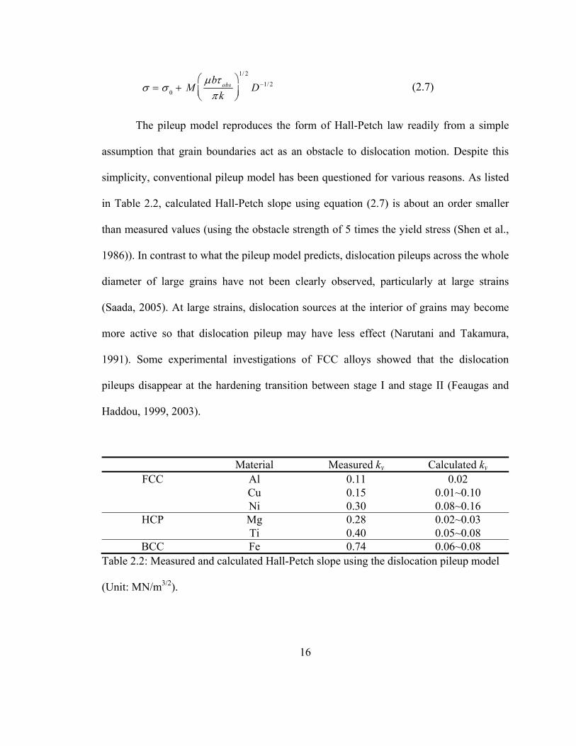
simplicity, conventional pileup model has been questioned for various reasons. As listed

in Table 2.2, calculated Hall-Petch slope using equation (2.7) is about an order smaller

than measured values (using the obstacle strength of 5 times the yield stress (Shen et al.,

1986)). In contrast to what the pileup model predicts, dislocation pileups across the whole

diameter of large grains have not been clearly observed, particularly at large strains

(Saada, 2005). At large strains, dislocation sources at the interior of grains may become

more active so that dislocation pileup may have less effect (Narutani and Takamura,

1991). Some experimental investigations of FCC alloys showed that the dislocation

pileups disappear at the hardening transition between stage I and stage II (Feaugas and

Haddou, 1999, 2003).

Material Measured ky Calculated ky FCC Al 0.11 0.02

Cu 0.15 0.01~0.10 Ni 0.30 0.08~0.16

HCP Mg 0.28 0.02~0.03 Ti 0.40 0.05~0.08

BCC Fe 0.74 0.06~0.08 Table 2.2: Measured and calculated Hall-Petch slope using the dislocation pileup model

(Unit: MN/m3/2).

17

The pileup of dislocation has been seldom observed in pure metals with high

stacking fault energy (Li and Chou, 1970) since cross-slip can occur easily near the grain

boundary. Hence, these metals are expected to have a relatively low Hall-Petch slope.

However, BCC metals tend to have higher Hall-Petch slope despite higher stacking fault

energy compared to FCC metals. This cannot be readily explained in terms of the pileup

model.

Also, equation (2.6) is only applicable when the number of dislocations in the

pileup is large enough that their distributions can be described by a continuous density

function. At smaller length scales, the effect of discrete dislocations has to be taken into

account (Fang and Friedman, 2007). In addition, grain boundary structure should be

introduced in the pileup models through appropriate expressions of grain boundary

obstacle strength.

The dislocation density model, or the work hardening model, is based on an

assumption that flow stress is proportional to the square root of dislocation density

(Conrad, 1961, 1970, 2004; Li, 1963a; Ashby, 1970; Chia et al., 2005). The flow stress is

given by

Mb (2.8)

where M is the average Taylor factor and α is a constant. Hall-Petch relation can be

readily derived from dislocation density model by assuming dislocation density is

inversely proportional to the grain size. Inversely proportional relation between the

dislocation density and the grain size is supported by TEM observations (Keh, 1961;

18

Conrad et al., 1968; Evans and Rawlings, 1969; Chia et al., 2005) and electrical

resistivity tests (Narutani and Takamura, 1991).

It has been proposed that the grain boundaries act as a dislocation source and

these emitted dislocations increase forest dislocation density and the overall flow stress

(Mott, 1946; Li, 1962). TEM observations have shown that dislocations are emitted from

the ledges (Mascanzoni and Buzzichelli, 1970; Murr, 1981) and Li (Li, 1961, 1963b)

proposed correlation between ky and the density of grain boundary source, e.g. ky is

proportional to square root of ledge density. However, various experimental observations

contradict to Li’s model. For instance, it has been reported that the pure nickel showed

linear relation between ky and ledge densities (Venkatesh and Murr, 1978) or no clear

correlation has been established between yk and the density of ledges (Bernstein and

Rath, 1973). Also, discrete dislocation simulations showed that source density and

location have a negligible effect on the Hall-Petch relation (Biner and Morris, 2003).

Ashby (Ashby, 1970) proposed two types of dislocations: the statistically stored

dislocations (SSD) and the geometrically necessary dislocations (GND). SSDs

correspond to the dislocations accumulated during a general, uniform deformation that is

randomly distributed over the entire grain while GNDs are the dislocations necessary to

avoid overlaps or voids near the grain boundaries during a local, non-uniform

deformation (Thompson et al., 1973). Statistically stored dislocation density ( S ) and

geometrically necessary dislocation density ( G ) are expressed as (Cottrell, 1953;

Ashby, 1970):

19

1S

s

C

b

2G

C

bD

(2.9)

where 1C and 2C are constants, s is the average slip length, D is the grain size and b is

the Burgers vector. The flow stress is then represented as follows:

1 20

' '( )

s

C C

D

(2.10)

Equation (2.10) shows similar form of D-1/2 dependence on the flow stress and

implies that the flow stress is increased by the reduction of the slip length and increase in

GND density necessary to maintain the material continuity across the grain boundaries

(Conrad, 1961, 1970). It should be noted that equation (2.10) reduces to Hall-Petch Law

if s D . The major difference between pileup model and dislocation density model is

the consideration of the dislocation arrangement and the effect of grain size on the total

dislocation density (Conrad, 2004). The dislocation density model predicts higher

dislocation density near the grain boundaries in terms of GNDs.

Another approach to describe the Hall-Petch Law is the composite model where

each grain is described as a composite material with the grain interior and the grain

boundary region which have different material properties (Kocks, 1970; Hirth, 1972;

Meyers and Ashworth, 1982). Using a simple law of mixture between two different

materials, overall flow stress is expressed as:

BULKf

GBff ff )1(

(2.11)

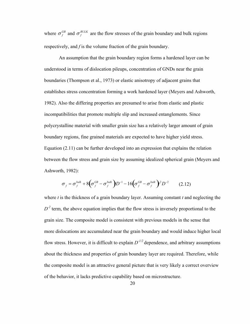
20

where GBf and BULK

f are the flow stresses of the grain boundary and bulk regions

respectively, and f is the volume fraction of the grain boundary.

An assumption that the grain boundary region forms a hardened layer can be

understood in terms of dislocation pileups, concentration of GNDs near the grain

boundaries (Thompson et al., 1973) or elastic anisotropy of adjacent grains that

establishes stress concentration forming a work hardened layer (Meyers and Ashworth,

1982). Also the differing properties are presumed to arise from elastic and plastic

incompatibilities that promote multiple slip and increased entanglements. Since

polycrystalline material with smaller grain size has a relatively larger amount of grain

boundary regions, fine grained materials are expected to have higher yield stress.

Equation (2.11) can be further developed into an expression that explains the relation

between the flow stress and grain size by assuming idealized spherical grain (Meyers and

Ashworth, 1982):

f

fbulk 8

fGB

fbulk tD1 16

fGB

fbulk t2D2

(2.12)

where t is the thickness of a grain boundary layer. Assuming constant t and neglecting the

D-2 term, the above equation implies that the flow stress is inversely proportional to the

grain size. The composite model is consistent with previous models in the sense that

more dislocations are accumulated near the grain boundary and would induce higher local

flow stress. However, it is difficult to explain D-1/2 dependence, and arbitrary assumptions

about the thickness and properties of grain boundary layer are required. Therefore, while

the composite model is an attractive general picture that is very likely a correct overview

of the behavior, it lacks predictive capability based on microstructure.

21

Although these models succeeded to reproduce the form of the Hall-Petch Law

based on simplifying assumptions, none of them seem to capture all the important

mechanisms near the grain boundaries. All models mentioned above lack connection to

the structure or orientation of the grain boundary, the actual slip systems, or the grain

misorientation, all of which are known to affect slip transmission at grain boundaries

(Shen et al., 1986; Wagoner et al., 1998). Therefore, it is difficult to conclude that the

actual mechanism will rigorously follow one of the proposed models but the actual

behavior near the grain boundary is likely to show mechanisms proposed by different

models and affected by the grain boundary structure, actual slip systems and grain

orientations. Hence, an integrated model that would encompass the effect of dislocation

interactions and grain boundary characteristics accurately describe and predict the Hall-

Petch relationship.

22

3. SINGLE CRYSTAL CONSTITUTIVE EQUATIONS

Note: Chapter 3 is presented in the format of a peer-reviewed paper that is accepted for

publication by the International Journal of Plasticity and is in press at this writing (Lee

et al., 2009).

3.1 Abstract

Single-crystal constitutive equations based on dislocation density (SCCE-D) were

developed from Orowan’s strengthening equation and simple geometric relationships of

the operating slip systems. The flow resistance on a slip plane was computed using the

Burger’s vector, line direction, and density of the dislocations on all other slip planes,

with no adjustable parameters. That is, the latent/ self-hardening matrix was determined

by the crystallography of the slip systems alone. The multiplication of dislocations on

each slip system incorporated standard 3-parameter dislocation-density evolution

equations applied to each slip system independently; this is the only phenomenological

aspect of the SCCE-D model. In contrast, the most widely used single-crystal constitutive

equations for texture analysis (SCCE-T) feature 4 or more adjustable parameters that are

usually back-fit from a polycrystal flow curve. In order to compare the accuracy of the

two approaches to reproduce single-crystal behavior, tensile tests of single crystals

oriented for single slip were simulated using crystal-plasticity finite element modeling.

23

Best-fit parameters (3 for SCCE-D, 4 for SCCE-T) were determined using either

multiple or single-slip stress-strain curves for copper and iron from the literature. Both

approaches reproduced the data used for fitting accurately. Tensile tests of copper and

iron single crystals oriented to favor the remaining combinations of slip systems were

then simulated using each model (i.e. multiple slip cases for equations fit to single slip,

and vice versa). In spite of fewer fit parameters, the SCCE-D predicted the flow stresses

with a standard deviation of 14 MPa, less than one half that for the SCCE-T conventional

equations: 31 MPa. Polycrystalline texture simulations were conducted to compare

predictions of the two models. The predicted polycrystal flow curves differed

considerably, but the differences in texture evolution were insensitive to the type of

constitutive equations. The SCCE-D method provides an improved representation of

single-crystal plastic response with fewer adjustable parameters, better accuracy, and

better predictivity than the constitutive equations most widely used for texture analysis

(SCCE-T).

3.2 Introduction

Modern “texture analysis” routinely predicts the plastic anisotropy and texture

evolution of polycrystals during large deformation, particularly for FCC crystal

structures. Such calculations make use of single-crystal constitutive equations based on

slip systems and statistical grain orientation information. The procedure does not consider

specific neighboring grain interactions or the presence of grain boundaries, as illustrated

in Figure 3.1. The linkage among grains in texture analyses is based on numerical

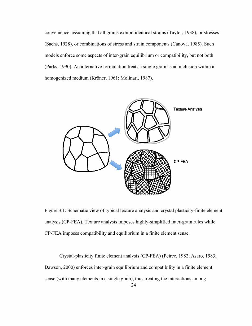
24

convenience, assuming that all grains exhibit identical strains (Taylor, 1938), or stresses

(Sachs, 1928), or combinations of stress and strain components (Canova, 1985). Such

models enforce some aspects of inter-grain equilibrium or compatibility, but not both

(Parks, 1990). An alternative formulation treats a single grain as an inclusion within a

homogenized medium (Kröner, 1961; Molinari, 1987).

Figure 3.1: Schematic view of typical texture analysis and crystal plasticity-finite element

analysis (CP-FEA). Texture analysis imposes highly-simplified inter-grain rules while

CP-FEA imposes compatibility and equilibrium in a finite element sense.

Crystal-plasticity finite element analysis (CP-FEA) (Peirce, 1982; Asaro, 1983;

Dawson, 2000) enforces inter-grain equilibrium and compatibility in a finite element

sense (with many elements in a single grain), thus treating the interactions among

25

neighboring grains more realistically (Raabe, 2002), Figure 3.1, but with large penalties

in computation time. Recent applications of CP-FEA have been extended to the

deformation of single, bi- and polycrystals (Zaefferer, 2003; Ma, 2006; Zaafarani, 2006;

Raabe, 2007), incorporatin size dependence through strain gradient terms (Abu Al-Rub,

2005) and nanoindentation simulations (Wang, 2004; Liu, 2005; Liu, 2008). These

methods are too CPU-intensive for use with large grain assemblies (i.e. typical

polycrystals) or for treating applied deformation boundary-value problems. Modifications

to improve the efficiency of the calculations limit the accuracy by, for example, applying

iso-strain conditions within a grain (Kalidindi, 1992; Dawson, 2003) or having each finite

element represent a single grain (Nakamachi, 2001).

Polycrystal simulations, whether of the texture type or CP-FEA type, use single

crystal plasticity constitutive models based on slip system activity. Typical formulations

are either elastic-plastic rate-independent (Mandel, 1965; Hill, 1966, 1972; Rice, 1971;

Asaro and Rice, 1977; Anand and Kothari, 1996; Marin and Dawson, 1998) or

viscoplastic (Peirce et al., 1982; Asaro and Needleman, 1985). This viscoplastic

approach has recently been referred to in the literature as “PAN” (e.g. (Alcalá et al.,

2008; Patil et al., 2008; Thakare et al., 2009)), named for “Peirce, Asaro, Needleman”

(Peirce et al., 1982; Asaro and Needleman, 1985). The PAN approach uses an arbitrary

small strain-rate sensitivity index to avoid numerical non-uniqueness. The most

commonly used PAN formulation relies on a power-law equation relating shear stress to

shear strain rate on each slip system (Asaro and Needleman, 1985) with the slip system

26

resistance evolving with total slip on each slip system according to latent and self-

hardening (Mandel, 1965; Hill, 1966).

The adjustable parameters in the single-crystal constitutive equations used for

texture analysis are almost universally determined by back-fitting them to mechanical test

results (i.e. uniaxial tension or compression) of macroscopic polycrystals that are

simulated using the same technique for which the constitutive equations are destined.

Such a procedure guarantees that the macroscopic tests used to fit the parameters are

reproduced accurately by the simulations, but not that the single-crystal constitutive

equations represent true single-crystal behavior. Simulations of problems based on such

an approach have proven useful for a range of strain, strain rates, and temperatures

(Mathur and Dawson, 1989; Bronkhorst et al., 1992; Beaudoin et al., 1994; Kumar and

Dawson, 1998; Nemat-Nasser et al., 1998). However, there is evidence that single-crystal

plasticity models fitted in this way do not always represent single-crystal behavior

properly (Becker and Panchanadeeswaran, 1995; Kumar and Yang, 1999; Arsenlis and

Parks, 2002). If the presence and characterization of grain boundaries (and grain shape,

size, misorientation, etc.) influences the relationship between single-crystal and

polycrystal deformation characteristics, the standard back-fitting procedure evidently

would not yield a correct description of single-crystal behavior. Instead, the single-crystal

constitutive equations embed undetermined aspects of the inter-grain interactions and

thus, may not represent single crystal behavior but rather some amalgam of single and

polycrystal aspects. One of the purposes of the current work is to determine whether the

predominant formulation of single-crystal constitutive equations used for a wide range of

27

successful texture calculations (“SCCE-T”) captures single crystal behavior properly,

particularly single slip vs. multiple slip. The answer to that question bears on the

question of whether inter-grain interactions are incorporated in an unknown way into the

SCCE-T’s fit to macroscopic observations.

Note: “SCCE-T” refers in this paper to a set of choices within the broader PAN

framework. It is SCCE-T that is used with wide success in texture calculations

appearing in the literature. SCCE-T is a subset of PAN, the latter of which has

greater flexibility with a commensurate number of additional adjustable parameters.

As a particular example, the majority of successful texture calculations use a fixed

value, 1.4, describing the ratio of latent hardening to self hardening that agrees with

experience at the macro/ texture level. SCCE-T, in addition to having the validation

of wide testing over more than 20 years, has only one additional parameter compared

with the constitutive model proposed here. Thus, comparisons between the two are

meaningful. Summaries of the constitutive forms considered in this paper are

presented later.

Alternate developments to represent single-crystal behavior based on dislocation

densities have appeared. Models of this type typically exhibit considerable complexity

and large numbers of undetermined parameters. Models based on statistical aspects of

dislocation densities represented as internal state variables (Ortiz et al., 1999; Arsenlis

and Parks, 2002) captured the orientation-dependent flow behavior of FCC single

crystals. Developments for FCC and BCC single crystals make use of Orowan’s equation

(Orowan, 1940) and have incorporated many physical complexities, including

28

dislocation velocities, activation energies, and dislocation walls (Roters et al., 2000). In

order to reproduce the compression of aluminum single crystals at elevated temperature,

8 fit parameters and 2 activation energies were required to predict stress strain curves for

a range of strain rates and temperatures in one study (Ma and Roters, 2004).

In the current work, a dislocation-based single crystal constitutive equation

(“SCCE-D”) is newly formulated with 3 undetermined parameters corresponding to a

standard equation representing the evolution of dislocation density. The form is similar to

standard corresponding texture-type equations, except that the dislocation density for

each slip system and its evolution is used explicitly rather than implicitly via slip system

strength and its evolution with total slip (Ortiz and Popov, 1982; Brown et al., 1989;

Kalidindi et al., 1992; Kuchnicki et al., 2006; Wang et al., 2007). Use of physical

dislocation densities allows application of Orowan’s strengthening model (Orowan,

1948) to determine the cross-hardening effects without undetermined parameters (see

also (Bassani and Wu, 1991) and (Liu et al., 2008)). Such cross-hardening effects

depend on the geometry of the crystal lattice type, not on undetermined parameters.

Tests of SCCE-D are made for single-crystal and polycrystal deformation and the

results are compared with corresponding ones using standard SCCE-T. We emphasize

that we have selected the SCCE-T for comparison with the new model because it

dominates successful texture calculations presented in the literature. As such, it

represents an informal “consensus” of what has been found to work. None of the other

variants within the PAN formalism approach the breadth of experience or acceptance in

the community. The question to be answered is whether the SCCE-T formulation that

29

finds broad success for polycrystal simulations represents single-crystal behavior

properly, and if not, whether a less-adjustable/ more predictive formulation can improve

on the single-crystal representation. A secondary question is how such an alternative

formulation would affect macroscopic texture calculations.

3.3 Crystal Plasticity based on Single Crystal Constitutive Equations

The kinematics for either SCCE-T or SCCE-D are based on well-established

developments (Lee, 1969; Rice, 1971; Hill and Rice, 1972; Asaro and Rice, 1977; Peirce

et al., 1982). The total deformation gradient is decomposed into elastic and plastic parts

(Lee, 1969):

e pF F F (3.1)

where Fe corresponds to elastic distortion of lattice, and Fp defines the slip by the

dislocation motion in the unrotated configuration (Mandel, 1965).

The plastic velocity gradient in the unrotated (or intermediate) configuration is:

p p p 1L F F (3.2)

The evolution of the plastic deformation can be expressed as the sum of all

crystallographic slip rates, (Rice, 1971),

np

0 01

L s n

(3.3)

where 0s and 0

n are the vectors representing slip direction and slip plane normal of the

slip system , respectively and n is total number of slip systems.

30

3.3.1 Common Elements of SCCE-T and SCCE-D

For a rate-dependent crystal plasticity model, the plastic shear rate of each slip

system is typically expressed as a power law function of the resolved shear stress as

(Hutchinson, 1976; Peirce et al., 1982):

1

0 signm

g

(3.4)

where 0 is reference shear rate, g is the slip resistance (or flow stress) of the slip

system and m is the rate sensitivity exponent. The initial flow stress is generally

assumed to be the same, i.e. 0g , for all slip systems. Reference shearing rate and rate

sensitivity, 0.001 s-1 and 0.012 respectively, are adopted from the literature (Bronkhorst

et al., 1992; Kalidindi et al., 1992).

To complete the constitutive equations, the second Piola-Kirchhoff stress is

defined as follows, and is related elastically to the strain:

S Ce:E det(Fe )Fe1FeT

(3.5)

where E 1

2FeTFe I is the Lagrangian strain tensor, is the Cauchy stress, and Ce

is the fourth order elastic constant matrix.

The resolved shear stress of slip system in equation (3.4) is approximately,

S : P0 S : s0

n0 or

0j0iij0ijij ns:SPS (3.6)

31

The slip resistance (equivalent to a critical resolved shear stress (CRSS) for a rate-

independent elastic-plastic law) of slip system , g evolves as the slip (or gliding) of

dislocations on the slip system occurs. The governing rule of the evolution of slip

resistance (hardening) is a critical aspect of the constitutive framework and causes the

SCCE-T and SCCE-D approaches to diverge, as described in the following sections.

3.3.2 Single-Crystal Constitutive Equations developed for Texture models

(SCCE-T)

Texture analyses predominantly utilize phenomenological models for the

evolution of flow stress on a slip system as related to the slip increment on all slip

systems as follows (Asaro, 1983):

g h

(3.7)

where h are hardening coefficients. Most texture analyses have adopted the following

form for the hardening coefficient matrix (Hutchinson, 1970; Asaro, 1979; Peirce et al.,

1982):

latselflat qqqhh (3.8)

where is the Kronecker delta and qself and qlat determine the self and latent hardening,

respectively. The hardening matrix contains two distinct values: diagonal terms (qself) for

the self-hardening and off-diagonal terms (qlat) for the latent hardening. Experimental

observations (Kocks, 1970) suggested that the range 1≤qlat /qself ≤1.4 applies for FCC

single crystals, and qlat / qself = 1.4 is typically used in texture analyses of FCC

32

polycrystals (Peirce et al., 1982; Asaro and Needleman, 1985; Mathur and Dawson, 1989;

Kalidindi et al., 1992).

The form of βh in equation (3.8) has been proposed to properly represent the

stress-strain behavior of polycrystals. Here, the widely-used form proposed by Brown et

al. (Brown et al., 1989) is adopted:

a

0 1hh

s

β

g

g

(3.9)

where h0 is the initial hardening rate, gs is the saturated flow stress and a is the hardening

exponent. The initial hardness g0 is typically fitted to reproduce the macroscopic yield

stress. Equations (3.7)-(3.9) have been shown to predict the stress-strain response and

evolution of texture for simple deformation of FCC polycrystals (Mathur and Dawson,

1989; Kalidindi et al., 1992). When the parameters are back-fitted to stress-strain

responses of polycrystals, there are 4 arbitrary parameters to be fit from macroscopic

polycrystal stress-strain curves to complete equations (3.7)-(3.9): h0, gs, g0 and a in

equations (3.4), (3.8) and (3.9). These undetermined parameters, h0, gs, g0, and a are

typically set from the stress strain curve for a polycrystal tensile test.

3.3.3 Single-Crystal Constitutive Equations based on the Dislocation density

model (SCCE-D)

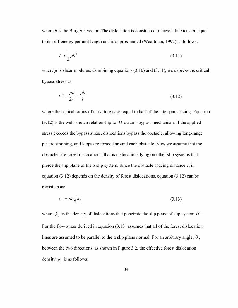
In the SCCE-D derived here, the hardening is expressed in terms of the interaction

of mobile dislocations with corresponding forest dislocations that act as point obstacles,

Figure 3.2. These interactions are evaluated using Orowan’s strengthening model

33

assuming that forest dislocations are hard pins with respect to intersecting mobile

dislocation. That is, the intersection points become immobile and the mobile dislocation

must bypass by looping around the obstacle rather than cutting through it. In fact,

dislocation intersections are known to be hard pins in most metals at low homologous

temperatures (Hirth and Lothe, 1969).

Forest dislocation

Active (moving) dislocation

Slip planeq

n(a)

Figure 3.2: Interaction between a moving dislocation on an active slip system and

corresponding forest dislocation array.

In Orowan’s model (Orowan, 1948), if the applied stress is large enough,

dislocations loop around an obstacle and will overcome and bypass it, leaving dislocation

loops behind. The critical stress ( g ) necessary to bow out a dislocation on a slip system

α to a radius r is calculated by considering the equilibrium with the line tension of the

dislocation, T:

r

Tbgα

(3.10)

34

where b is the Burger’s vector. The dislocation is considered to have a line tension equal

to its self-energy per unit length and is approximated (Weertman, 1992) as follows:

2

2

1μbT

(3.11)

where is shear modulus. Combining equations (3.10) and (3.11), we express the critical

bypass stress as

l

μb

r

μbgα

2

(3.12)

where the critical radius of curvature is set equal to half of the inter-pin spacing. Equation

(3.12) is the well-known relationship for Orowan’s bypass mechanism. If the applied

stress exceeds the bypass stress, dislocations bypass the obstacle, allowing long-range

plastic straining, and loops are formed around each obstacle. Now we assume that the

obstacles are forest dislocations, that is dislocations lying on other slip systems that

pierce the slip plane of the α slip system. Since the obstacle spacing distance l, in

equation (3.12) depends on the density of forest dislocations, equation (3.12) can be

rewritten as:

fα ρμbg

(3.13)

where fρ is the density of dislocations that penetrate the slip plane of slip system .

For the flow stress derived in equation (3.13) assumes that all of the forest dislocation

lines are assumed to be parallel to the α slip plane normal. For an arbitrary angle, ,

between the two directions, as shown in Figure 3.2, the effective forest dislocation

density fρ is as follows:

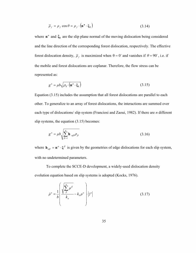
35

fα ξn fff ρθρρ cos

(3.14)

where αn and fξ are the slip plane normal of the moving dislocation being considered

and the line direction of the corresponding forest dislocation, respectively. The effective

forest dislocation density, fρ is maximized when 0θ and vanishes if 90θ , i.e. if

the mobile and forest dislocations are coplanar. Therefore, the flow stress can be

represented as:

ff ξn μbg α

(3.15)

Equation (3.15) includes the assumption that all forest dislocations are parallel to each

other. To generalize to an array of forest dislocations, the interactions are summed over

each type of dislocations/ slip system (Franciosi and Zaoui, 1982). If there are n different

slip systems, the equation (3.15) becomes:

n

α μbg1

h

(3.16)

where ξnh is given by the geometries of edge dislocations for each slip system,

with no undetermined parameters.

To complete the SCCE-D development, a widely-used dislocation density

evolution equation based on slip systems is adopted (Kocks, 1976).

ααb

a

n

β

β

α γρkk

ρ

bρ

1

(3.17)

36

where ka and kb are material parameters for the generation and annihilation terms of

dislocations, respectively. The final SCCE-D defined by equations (3.16) and (3.17) has

three parameters to be determined, each of them related to dislocation density and its

evolution: ka, kb and 0. In order to compare the accuracy and usefulness of SCCE-T and

SCCE-D as described above, the adjustable parameters were fit to reproduce the

measured stress-strain response of single crystals oriented for either multiple or single

slip. The resulting material models were then used with finite element modeling to

predict the stress-strain response for tensile tests oriented for the activation of other

combinations of slip systems. The predicted responses were then compared with

corresponding experimental results from the literature.

3.4 CP-FEM Implementation

The two single-crystal constitutive equations described in the previous section

were implemented into the commercial finite element program ABAQUS/Standard via

the user material subroutine, UMAT (Hibbit, 2005). A single eight-noded continuum

element (C3D8) was utilized to simulate the tensile tests of single crystals. The tensile

direction was aligned with one of the element axes and the two faces of the cube element

were initially perpendicular to the loading axis. During the deformation, the two faces

remain parallel to each other and perpendicular to the loading axis, simulating the

deformation mode imposed by a stiff tensile machine. Crystallographic slip was

considered on the 12 equivalent {111} 110 slip systems for FCC copper and 12

{110} 111 and 12 {112} 111 slip systems for BCC iron.

37

The tensile stress-strain responses for oriented single crystals have been

measured. For FCC copper single crystals, 4 tensile axis orientations are available

(Takeuchi, 1975; Arsenlis and Parks, 2002): <123>, <112>, <100>, and <111>. The

<123> tensile axis is oriented for single slip while <112>, <111> and <100> tensile axes

are oriented for multiple slip, with 2, 6 and 8 equally favored slip systems respectively.

For BCC iron single crystals, 3 tensile axis orientations are available (Keh, 1965): <348>,

<110>, and <100>. The <348> tensile axis is oriented for single slip while the <110>

and <100> tensile axes are orientated for multiple slip, with 2 and 4 equally favored slip

systems respectively.

3.5 Prediction of Single Crystal Stress-strain Response

SCCE-T and SCCE-D models were fit by comparing FE simulations of single-

crystal tensile tests oriented along directions with most equivalent slip systems, [001],

with corresponding experimental stress-strain curves from the literature. The best-fit

parameters, Table 3.1, were determined using the procedure described below. The stress-

strain responses for other orientations of tensile axis were then predicted using the

resulting constitutive equations. For SCCE-T, 0h affects the initial hardening rate, sg

determines the final saturated value of stress, 0g determines initial yield and a affects the

shape of the stress-strain curve (Kalidindi et al., 1992). For SCCE-D, 0 corresponds to

0g for SCCE-T, which determines the yield stress while ak and bk affect the shape of

the flow curve.

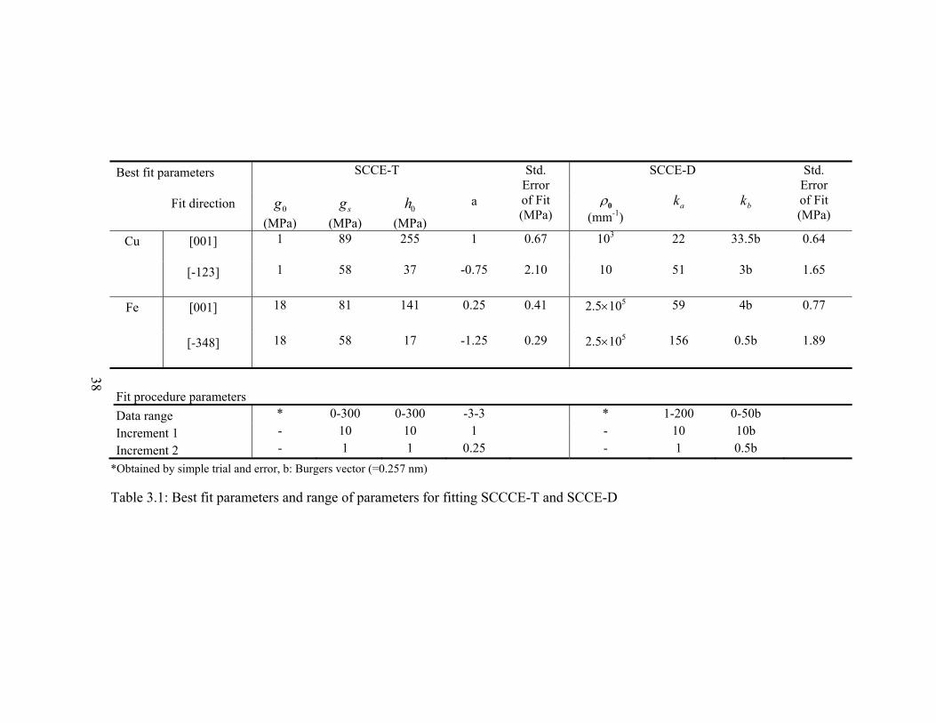
38

Best fit parameters SCCE-T Std. Error of Fit (MPa)

SCCE-D Std. Error of Fit (MPa)

Fit direction 0g

(MPa) sg

(MPa) 0h

(MPa)

a 0

(mm-1) ka kb

Cu [001] 1 89 255 1 0.67 103 22 33.5b 0.64

[-123] 1 58 37 -0.75 2.10 10 51 3b 1.65

Fe [001] 18 81 141 0.25 0.41 2.5105 59 4b 0.77

[-348] 18 58 17 -1.25 0.29 2.5105 156 0.5b 1.89

Fit procedure parameters

Data range * 0-300 0-300 -3-3 * 1-200 0-50b

Increment 1 - 10 10 1 - 10 10b

Increment 2 - 1 1 0.25 - 1 0.5b

*Obtained by simple trial and error, b: Burgers vector (=0.257 nm)

Table 3.1: Best fit parameters and range of parameters for fitting SCCCE-T and SCCE-D

38

39

In order to determine the set of parameters with minimum standard error of fit, 0g

for SCCE-T and 0 for SCCE-D were first obtained from the observed yield stress by

simple trial and error. Then, a 3-D “box” containing an assumed range of all possible

combinations of parameters was constructed, along with equally-spaced interior points.

Using SCCE-T as an example, 6727 equally-spaced interior points (i.e. 31×31×7)

representing 6727 choices of constitutive parameters was considered with ranges and

increments as defined in Table 3.1: Best fit parameters and range of parameters for fitting

SCCCE-T and SCCE-D (Increment 1). The following steps were then followed:

1. For each of the 6727 choices, a finite element analysis was performed and a standard

deviation of stress from the simulation and experiments was determined up to a strain

of 0.1. The set of parameters representing the minimum standard deviation was

identified for further refinement.

2. The behavior of the standard deviation moving along any parametric axis was

examined. For all the cases considered here, the standard deviation increased

monotonically in all such directions moving away from the minimum standard

deviation set identified in Step 1.

3. Starting from the set of parameters identified in Step 1, a smaller set of increments

(Increment 2 in Table 3.1) was used to define 3969 (21×21×9) new sets of parameters

throughout a range that includes the original cells adjacent to the location of the

minimum standard deviation. Step 1 was again carried out using these choices, and

the minimum standard deviation was thus refined. Again, the standard deviation was

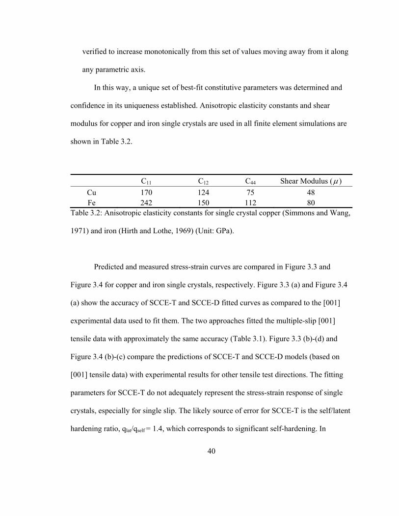
40

verified to increase monotonically from this set of values moving away from it along

any parametric axis.

In this way, a unique set of best-fit constitutive parameters was determined and

confidence in its uniqueness established. Anisotropic elasticity constants and shear

modulus for copper and iron single crystals are used in all finite element simulations are

shown in Table 3.2.

C11 C12 C44 Shear Modulus ( )

Cu 170 124 75 48 Fe 242 150 112 80

Table 3.2: Anisotropic elasticity constants for single crystal copper (Simmons and Wang,

1971) and iron (Hirth and Lothe, 1969) (Unit: GPa).

Predicted and measured stress-strain curves are compared in Figure 3.3 and

Figure 3.4 for copper and iron single crystals, respectively. Figure 3.3 (a) and Figure 3.4

(a) show the accuracy of SCCE-T and SCCE-D fitted curves as compared to the [001]

experimental data used to fit them. The two approaches fitted the multiple-slip [001]

tensile data with approximately the same accuracy (Table 3.1). Figure 3.3 (b)-(d) and

Figure 3.4 (b)-(c) compare the predictions of SCCE-T and SCCE-D models (based on

[001] tensile data) with experimental results for other tensile test directions. The fitting

parameters for SCCE-T do not adequately represent the stress-strain response of single

crystals, especially for single slip. The likely source of error for SCCE-T is the self/latent

hardening ratio, qlat/qself = 1.4, which corresponds to significant self-hardening. In

41

contrast, the measured hardening rate of the stress-strain curve oriented for single slip is

very low, implying negligible self-hardening.*

Engineering Strain

0.00 0.02 0.04 0.06 0.08 0.10

En

gin

eeri

ng

Str

ess

(MP

a)

0

50

100

150

200

250

Measured SCCE-T (Fit)SCCE-D (Fit)

Cu [001] (Takeuchi, 1975)(8 equal slip systems)

(a)

Continued

Figure 3.3: Comparison of stress-strain curves from SCCE-T and SCCE-D constitutive

models and measurements from the literature (Takeuchi, 1975) for copper single crystals

with tensile axes in the following orientations: (a) [001] (b) [-111] (c) [-112] (d) [-123].

The parameters for the SCCE-T and SCCE-D constitutive models have been fitted to the

[001] tensile test results, as shown in part (a).

* There is some hardening in single slip orientations even without self hardening because of the

rotation of the crystallographic direction relative to the tensile axis toward a less favorable slip

orientations (Anand, 1996)

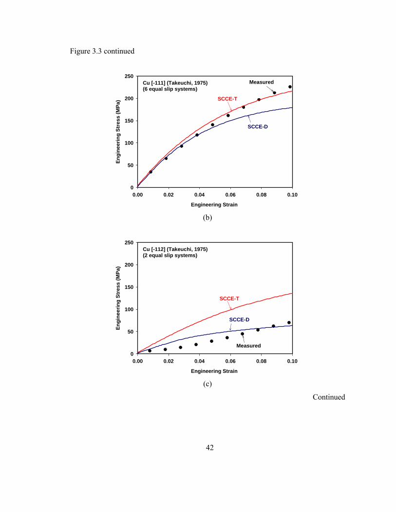
42

Figure 3.3 continued

Engineering Strain

0.00 0.02 0.04 0.06 0.08 0.10

En

gin

eer

ing

Str

ess

(M

Pa

)

0

50

100

150

200

250Cu [-111] (Takeuchi, 1975)(6 equal slip systems)

SCCE-D

SCCE-T

Measured

(b)

Engineering Strain

0.00 0.02 0.04 0.06 0.08 0.10

En

gin

eeri

ng

Str

ess

(MP

a)

0

50

100

150

200

250Cu [-112] (Takeuchi, 1975)(2 equal slip systems)

SCCE-D

SCCE-T

Measured

(c)

Continued

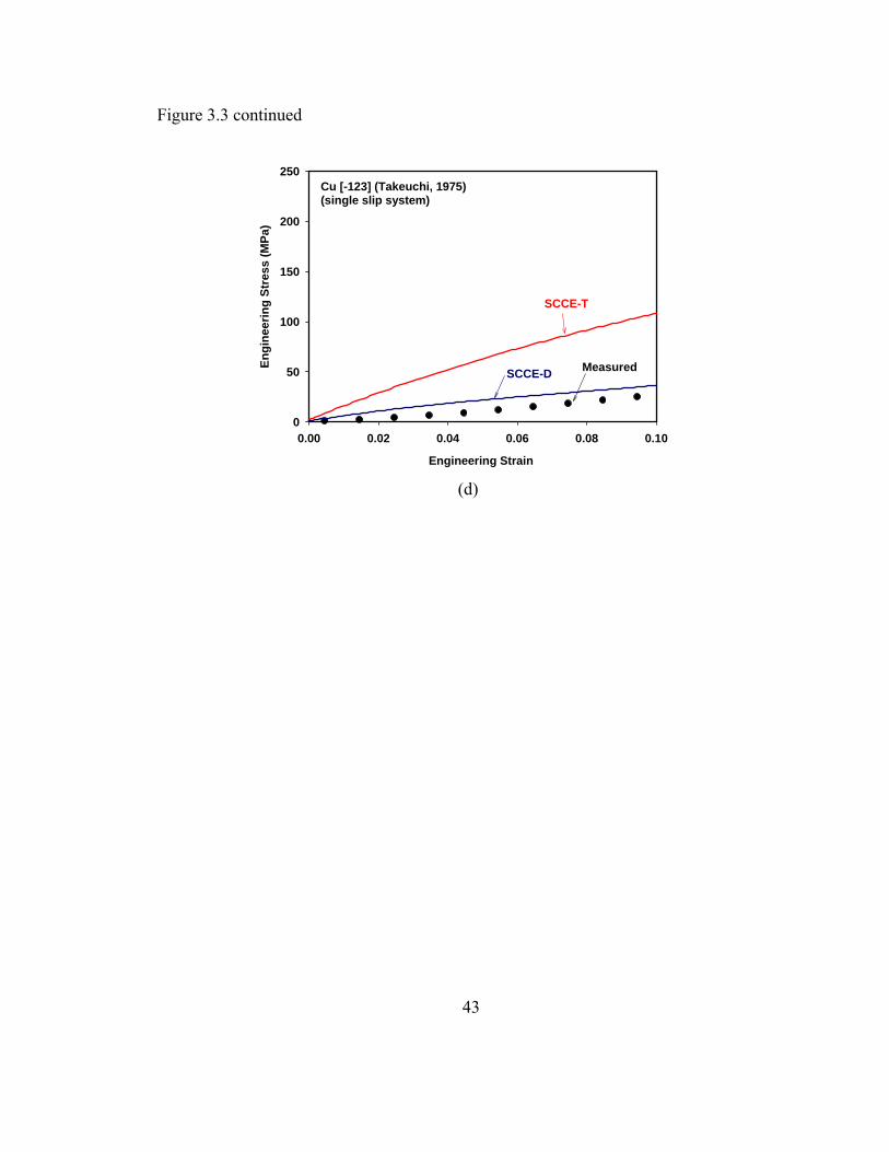
43

Figure 3.3 continued

Engineering Strain

0.00 0.02 0.04 0.06 0.08 0.10

En

gin

eeri

ng

Str

ess

(MP

a)

0

50

100

150

200

250Cu [-123] (Takeuchi, 1975)(single slip system)

SCCE-D

SCCE-T

Measured

(d)

44

Engineering Strain

0.00 0.02 0.04 0.06 0.08 0.10

En

gin

eeri

ng

Str

ess

(MP

a)

0

50

100

150

200

Measured SCCE-T (Fit)SCCE-D (Fit)

Fe [001] (Keh, 1964)(4 equal slip systems)

(a)

Continued

Figure 3.4: Comparison of stress-strain curves from SCCE-T and SCCE-D constitutive

models and measurements from the literature (Keh, 1965) for iron single crystals with

tensile axes in the following orientations: (a) [001] (b) [011] (c) [-348]. The parameters

for the SCCE-T and SCCE-D constitutive models have been fitted to the [001] tensile test

results, as shown in part (a).

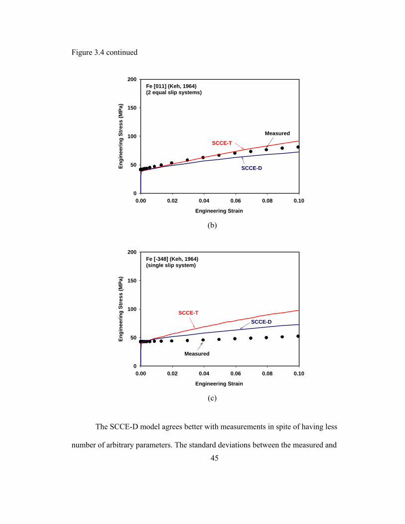
45

Figure 3.4 continued

Engineering Strain

0.00 0.02 0.04 0.06 0.08 0.10

En

gin

eeri

ng

Str

ess

(MP

a)

0

50

100

150

200Fe [011] (Keh, 1964)(2 equal slip systems)

SCCE-D

SCCE-T

Measured

(b)

Engineering Strain

0.00 0.02 0.04 0.06 0.08 0.10

En

gin

eeri

ng

Str

ess

(MP

a)

0

50

100

150

200Fe [-348] (Keh, 1964)(single slip system)

SCCE-D

SCCE-T

Measured

(c)

The SCCE-D model agrees better with measurements in spite of having less

number of arbitrary parameters. The standard deviations between the measured and

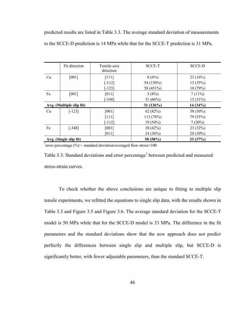
46

predicted results are listed in Table 3.3. The average standard deviation of measurements

to the SCCE-D prediction is 14 MPa while that for the SCCE-T prediction is 31 MPa.

Fit direction Tensile axis direction

SCCE-T SCCE-D

Cu [001] [111] 8 (6%) 23 (16%) [-112] 54 (150%) 13 (35%) [-123] 58 (451%) 10 (79%)

Fe [001] [011] 5 (8%) 7 (11%) [-348] 31 (66%) 15 (31%)

Avg. (Multiple slip fit) 31 (136%) 14 (34%)

Cu [-123] [001] 62 (82%) 38 (50%) [111] 113 (78%) 79 (55%) [-112] 19 (54%) 7 (20%)

Fe [-348] [001] 30 (42%) 23 (32%) [011] 24 (36%) 20 (30%)

Avg. (Single slip fit) 50 (58%) 33 (37%) 1error percentage (%) = standard deviation/averaged flow stress×100

Table 3.3: Standard deviations and error percentage1 between predicted and measured

stress-strain curves.

To check whether the above conclusions are unique to fitting to multiple slip

tensile experiments, we refitted the equations to single slip data, with the results shown in

Table 3.3 and Figure 3.5 and Figure 3.6. The average standard deviation for the SCCE-T

model is 50 MPa while that for the SCCE-D model is 33 MPa. The difference in the fit

parameters and the standard deviations show that the new approach does not predict

perfectly the differences between single slip and multiple slip, but SCCE-D is

significantly better, with fewer adjustable parameters, than the standard SCCE-T.

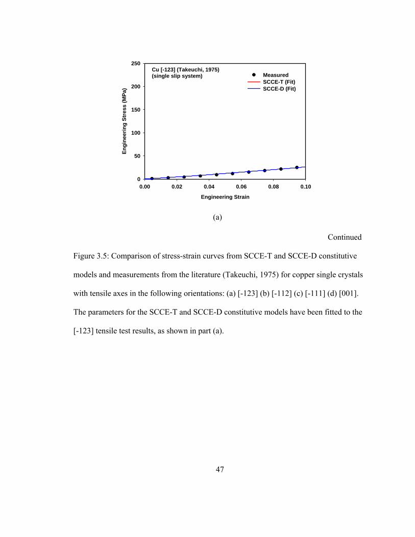
47

Engineering Strain

0.00 0.02 0.04 0.06 0.08 0.10

En

gin

eeri

ng

Str

ess

(M

Pa)

0

50

100

150

200

250

Measured SCCE-T (Fit)SCCE-D (Fit)

Cu [-123] (Takeuchi, 1975)(single slip system)

(a)

Continued

Figure 3.5: Comparison of stress-strain curves from SCCE-T and SCCE-D constitutive

models and measurements from the literature (Takeuchi, 1975) for copper single crystals

with tensile axes in the following orientations: (a) [-123] (b) [-112] (c) [-111] (d) [001].

The parameters for the SCCE-T and SCCE-D constitutive models have been fitted to the

[-123] tensile test results, as shown in part (a).

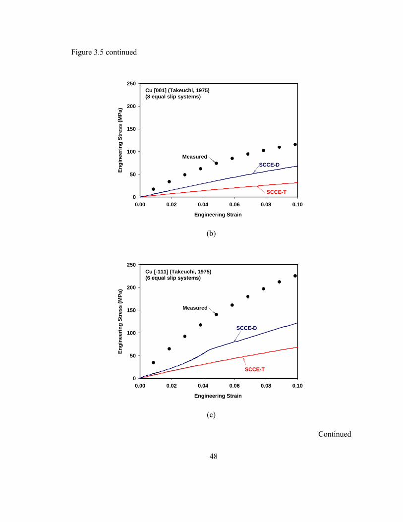
48

Figure 3.5 continued

Engineering Strain

0.00 0.02 0.04 0.06 0.08 0.10

En

gin

eeri

ng

Str

ess

(MP

a)

0

50

100

150

200

250Cu [001] (Takeuchi, 1975)(8 equal slip systems)

SCCE-D

SCCE-T

Measured

(b)

Engineering Strain

0.00 0.02 0.04 0.06 0.08 0.10

En

gin

eeri

ng

Str

ess

(MP

a)

0

50

100

150

200

250Cu [-111] (Takeuchi, 1975)(6 equal slip systems)

SCCE-D

SCCE-T

Measured

(c)

Continued

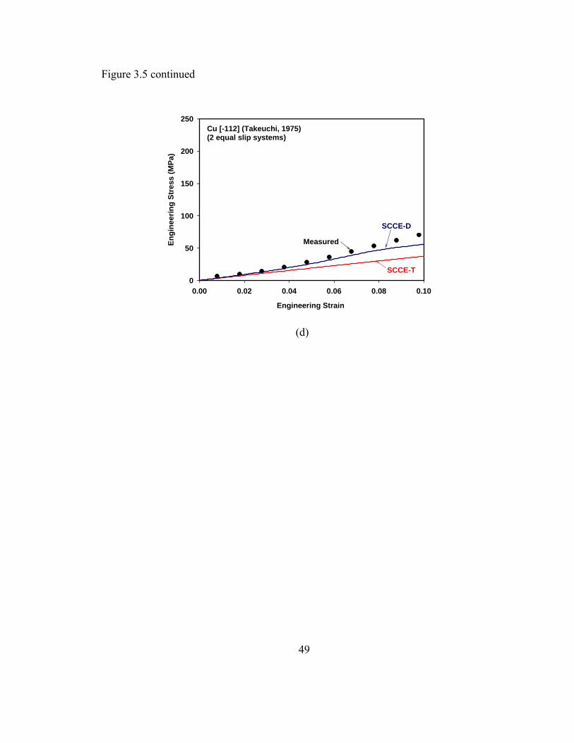
49

Figure 3.5 continued

Engineering Strain

0.00 0.02 0.04 0.06 0.08 0.10

En

gin

eeri

ng

Str

ess

(MP

a)

0

50

100

150

200

250Cu [-112] (Takeuchi, 1975)(2 equal slip systems)

SCCE-D

SCCE-T

Measured

(d)

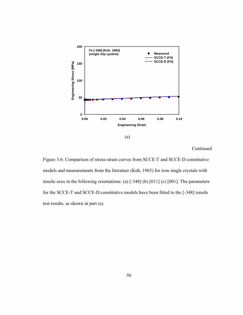
50

Engineering Strain

0.00 0.02 0.04 0.06 0.08 0.10

En

gin

eeri

ng

Str

ess

(M

Pa

)

0

50

100

150

200

Measured SCCE-T (Fit)SCCE-D (Fit)

Fe [-348] (Keh, 1964)(single slip system)

(a)

Continued

Figure 3.6: Comparison of stress-strain curves from SCCE-T and SCCE-D constitutive

models and measurements from the literature (Keh, 1965) for iron single crystals with

tensile axes in the following orientations: (a) [-348] (b) [011] (c) [001]. The parameters

for the SCCE-T and SCCE-D constitutive models have been fitted to the [-348] tensile

test results, as shown in part (a).

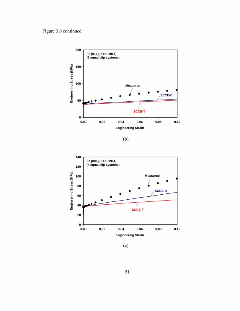
51

Figure 3.6 continued

Engineering Strain

0.00 0.02 0.04 0.06 0.08 0.10

En

gin

eeri

ng

Str

ess

(MP

a)

0

50

100

150

200Fe [011] (Keh, 1964)(2 equal slip systems)

SCCE-D

SCCE-T

Measured

(b)

Engineering Strain

0.00 0.02 0.04 0.06 0.08 0.10

En

gin

eeri

ng

Str

ess

(MP

a)

0

20

40

60

80

100

120

140Fe [001] (Keh, 1964)(4 equal slip systems)

SCCE-D

SCCE-T

Measured

(c)

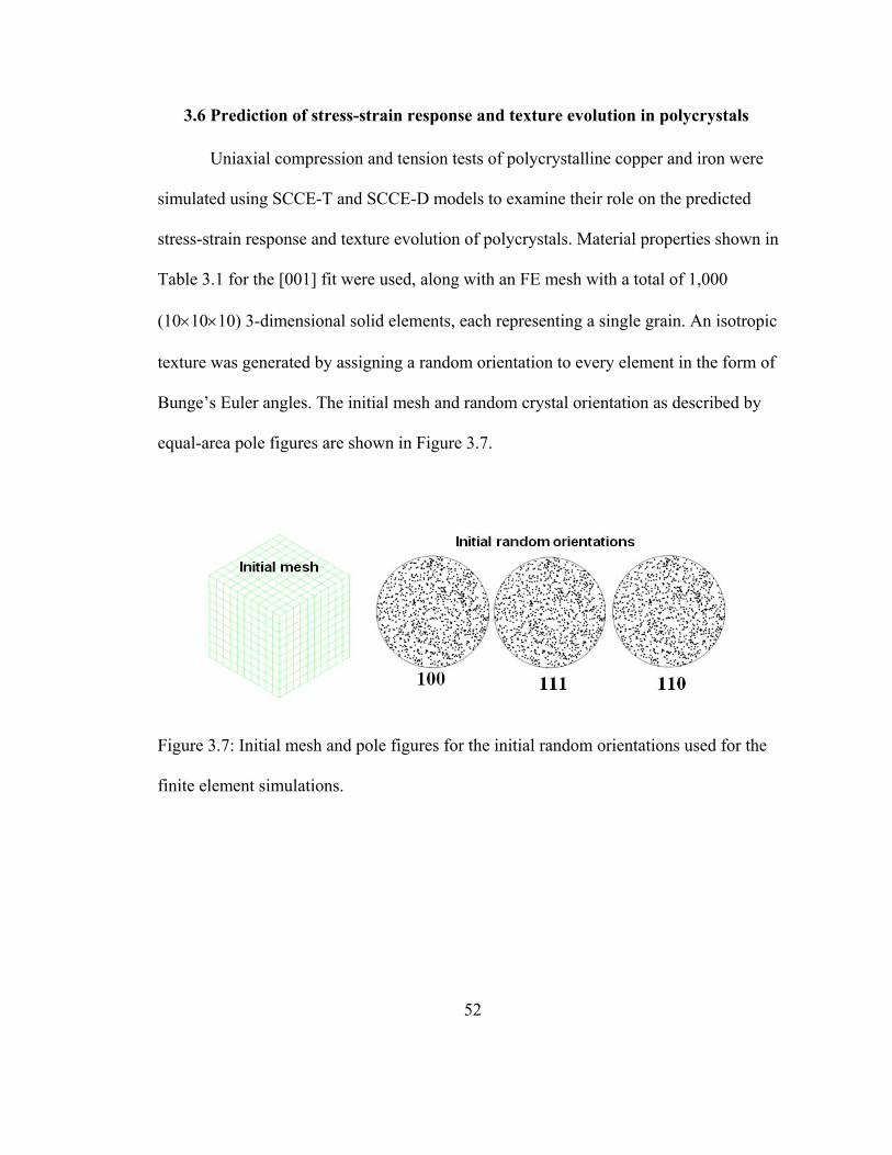
52

3.6 Prediction of stress-strain response and texture evolution in polycrystals

Uniaxial compression and tension tests of polycrystalline copper and iron were

simulated using SCCE-T and SCCE-D models to examine their role on the predicted

stress-strain response and texture evolution of polycrystals. Material properties shown in

Table 3.1 for the [001] fit were used, along with an FE mesh with a total of 1,000

(101010) 3-dimensional solid elements, each representing a single grain. An isotropic

texture was generated by assigning a random orientation to every element in the form of

Bunge’s Euler angles. The initial mesh and random crystal orientation as described by

equal-area pole figures are shown in Figure 3.7.

Figure 3.7: Initial mesh and pole figures for the initial random orientations used for the

finite element simulations.

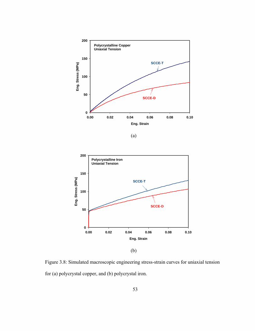
53

Eng. Strain

0.00 0.02 0.04 0.06 0.08 0.10

En

g. S

tre

ss (

MP

a)

0

50

100

150

200

SCCE-T

SCCE-D

Polycrystalline CopperUniaxial Tension

(a)

Eng. Strain

0.00 0.02 0.04 0.06 0.08 0.10

En

g. S

tre

ss (

MP

a)

0

50

100

150

200

SCCE-T

SCCE-D

Polycrystalline IronUniaxial Tension

(b)

Figure 3.8: Simulated macroscopic engineering stress-strain curves for uniaxial tension

for (a) polycrystal copper, and (b) polycrystal iron.

54

Eng. Strain

0.00 0.02 0.04 0.06 0.08 0.10

En

g. S

tre

ss (

MP

a)

0

50

100

150

200

250

300

SCCE-T

SCCE-D

Polycrystalline CopperUniaxial Compression

(a)

Eng. Strain

0.00 0.02 0.04 0.06 0.08 0.10

En

g. S

tre

ss (

MP

a)

0

50

100

150

200

SCCE-T

SCCE-D

Polycrystalline IronUniaxial Compression

(b)

Figure 3.9: Simulated macroscopic engineering stress-strain curves for uniaxial

compression for (a) polycrystal copper, and (b) polycrystal iron.

55

Figure 3.8 and Figure 3.9 show the simulated stress-strain curves for the SCCE-T

model and the SCCE-D model for copper and iron polycrystals. The SCCE-T prediction

for both copper and iron polycrystals shows higher flow stresses than SCCE-D

predictions throughout the tested strain range. Recall that both constitutive models were

fit to single crystals oriented for multiple slip. As Figure 3.3 and Figure 3.4 illustrate, the

SCCE-T model over-predicts the single crystal tensile flow stress for single slip and cases

having limited numbers of slip systems. This over-prediction is apparently important for

large polycrystal arrays; that is, regions of single or limited numbers of slip systems must

still be present, thereby influencing the observed macro behavior, for macroscopic

applied strains up to 0.1.

56

SCCE-T SCCE-D

(a)

SCCE-T SCCE-D

(b)

Figure 3.10: Equal area projection pole figures after 50% tension; (a) {110} pole figure

for copper, and (b) {111} pole figure for iron.

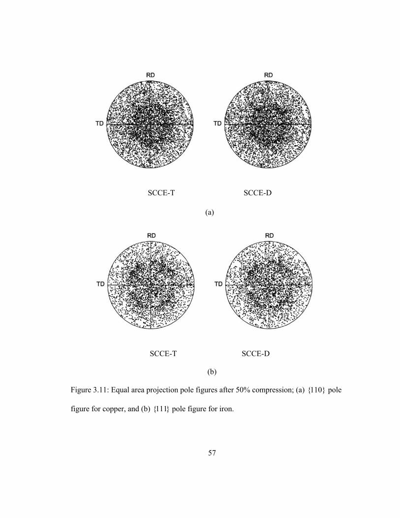
57

SCCE-T SCCE-D

(a)

SCCE-T SCCE-D

(b)

Figure 3.11: Equal area projection pole figures after 50% compression; (a) {110} pole

figure for copper, and (b) {111} pole figure for iron.

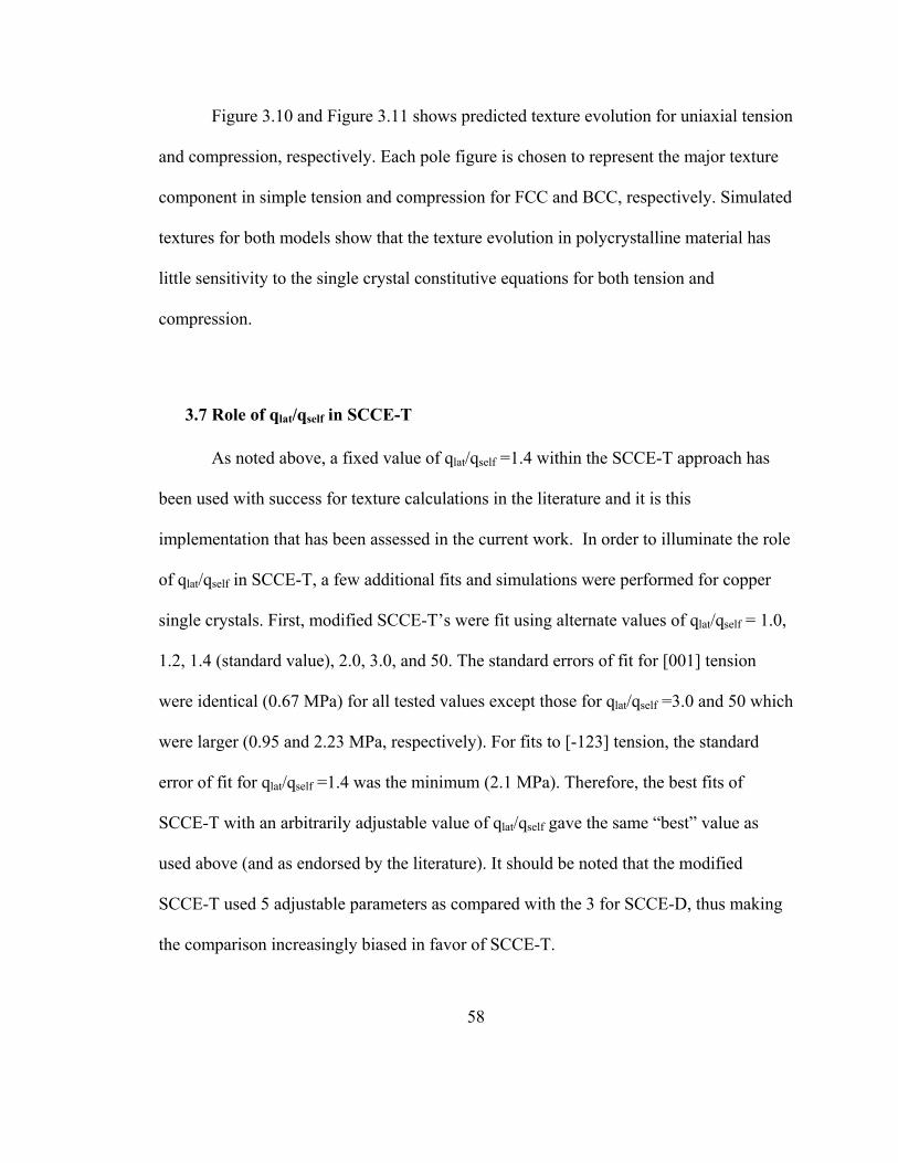
58

Figure 3.10 and Figure 3.11 shows predicted texture evolution for uniaxial tension

and compression, respectively. Each pole figure is chosen to represent the major texture

component in simple tension and compression for FCC and BCC, respectively. Simulated

textures for both models show that the texture evolution in polycrystalline material has

little sensitivity to the single crystal constitutive equations for both tension and

compression.

3.7 Role of qlat/qself in SCCE-T

As noted above, a fixed value of qlat/qself =1.4 within the SCCE-T approach has

been used with success for texture calculations in the literature and it is this

implementation that has been assessed in the current work. In order to illuminate the role

of qlat/qself in SCCE-T, a few additional fits and simulations were performed for copper

single crystals. First, modified SCCE-T’s were fit using alternate values of qlat/qself = 1.0,

1.2, 1.4 (standard value), 2.0, 3.0, and 50. The standard errors of fit for [001] tension

were identical (0.67 MPa) for all tested values except those for qlat/qself =3.0 and 50 which

were larger (0.95 and 2.23 MPa, respectively). For fits to [-123] tension, the standard

error of fit for qlat/qself =1.4 was the minimum (2.1 MPa). Therefore, the best fits of

SCCE-T with an arbitrarily adjustable value of qlat/qself gave the same “best” value as

used above (and as endorsed by the literature). It should be noted that the modified

SCCE-T used 5 adjustable parameters as compared with the 3 for SCCE-D, thus making

the comparison increasingly biased in favor of SCCE-T.

59

As an extension of these tests, the various constitutive models (i.e. best-fit

parameters for each choice of qlat/qself) were then used to simulate tension tests carried out

in the direction not used for fitting. The standard deviations for [-123] tensile tests

simulated using the modified SCCE-T’s were 20 to 68 MPa (160-540%), as compared

with 10 MPa for SCCE-D (80%). The standard deviations for [001] tensile tests

simulated using the modified SCCE-T’s were 45 to 64 MPa (60-85%), as compared with

38 MPa for SCCE-D (50%). Thus, even using the more flexible SCCE-T with arbitrarily

adjustable qlat/qself (5 parameters) over a wide range of values did not match the accuracy

of the fit or predictions obtained with the proposed SCCE-D (3 parameters).

3.8 Conclusions

The following conclusions apply to comparisons of new Single Crystal

Constitutive Equations based on Dislocation Density (SCCE-D) and standard Single

Crystal Constitutive Equations for Texture Analysis (SCCE-T):

1) SCCE-D reproduce flow curves for single slip and multi slip adequately in

FCC and BCC single crystals. SCCE-D have better accuracy than SCCE-T while using

smaller number of adjustable parameters. The average standard deviation predicted by

SCCE-D is 14 MPa while that for the SCCE-T is 31 MPa.

2) SCCE-T, which are usually back-fitted from polycrystal flow curves, do not

adequately represent orientation - dependent single crystal behavior. The discrepancy

may arise from neglecting the effect of grain boundaries, grain size and relative

misorientations between grains.

60

3) Polycrystal simulations using SCCE-T fit to multiple slip single crystal data

predict higher flow stresses than SCCE-D, correlated with the high flow stresses

predicted by the former for single crystals oriented for limited slip system activation. This

correlation implies that there may exist significant regions of limited slip activation in

polycrystals, contrary to the usual assumption.

4) Texture evolution has little sensitivity to the type of constitutive equations.

Simulated textures for SCCE-T and SCCE-D for FCC and BCC polycrystals are similar,

while the simulated macroscopic stress-strain responses differ.

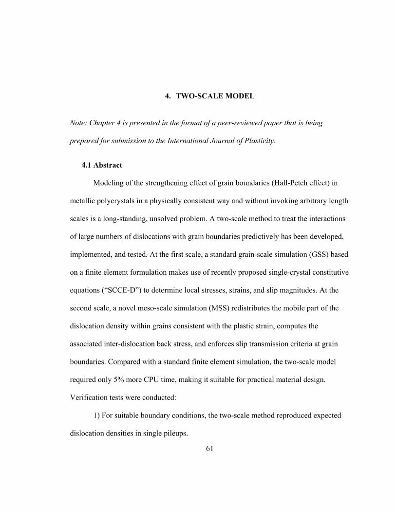
61

4. TWO-SCALE MODEL

Note: Chapter 4 is presented in the format of a peer-reviewed paper that is being

prepared for submission to the International Journal of Plasticity.

4.1 Abstract

Modeling of the strengthening effect of grain boundaries (Hall-Petch effect) in

metallic polycrystals in a physically consistent way and without invoking arbitrary length

scales is a long-standing, unsolved problem. A two-scale method to treat the interactions

of large numbers of dislocations with grain boundaries predictively has been developed,

implemented, and tested. At the first scale, a standard grain-scale simulation (GSS) based

on a finite element formulation makes use of recently proposed single-crystal constitutive

equations (“SCCE-D”) to determine local stresses, strains, and slip magnitudes. At the

second scale, a novel meso-scale simulation (MSS) redistributes the mobile part of the

dislocation density within grains consistent with the plastic strain, computes the

associated inter-dislocation back stress, and enforces slip transmission criteria at grain

boundaries. Compared with a standard finite element simulation, the two-scale model

required only 5% more CPU time, making it suitable for practical material design.

Verification tests were conducted:

1) For suitable boundary conditions, the two-scale method reproduced expected

dislocation densities in single pileups.

62

2) Tensile tests of iron multi-crystal specimens with 9 to 39 grains were

conducted and simulated using the two-scale model and four traditional models for

comparison: finite element model (GSS only) with either SCCE-D or PAN constitutive

models (PAN=Peirce, Asaro, Needleman) (Peirce et al. 1982; Asaro and Needleman,

1985), and Taylor model (Taylor, 1938) with either SCCE-D or PAN constitutive models.

The two-scale approach with SCCE-D predicted flow stresses 2-4 times more accurately

than the other method. None of the other methods predicted the Hall-Petch.

3) Two-scale simulations of 2D and 3D arrays of regular grains predicted Hall-

Petch slopes for iron of 1.2 ± 0.3 MN/m3/2 and 1.5 ± 0.3 MN/m3/2 , in agreements with a

measured slope of 0.9 ± 0.1 MN/m3/2.

4) The lattice curvature of a deformed Fe-3% Si columnar multicrystal was

predicted and measured. The maximum lattice curvature (near some grain boundaries)

agrees within the experimental scatter.

4.2 Introduction

Significant advances have been made in understanding the plastic behavior of

metals at two extreme length scales. At the atomic/single dislocation level, molecular

dynamics reveal how single dislocations move, how they are generated and annihilated in

small reference volumes on the order of thousands of atoms (Kubin et al., 1992; Zbib et

al., 1998; Schwarz, 1999), or in smaller volume elements to represent a single dislocation

(Acharya, 2001). Such methods apply to nano-structures but are difficult to scale up to

63

structures of multiple-micron size, such as are encountered in the grain sizes of typical

structural metals and alloys.

At the other extreme, macroscopic texture analysis of polycrystals predicts the

plastic anisotropy of textured sheets, particularly for FCC single-phase metals (Asaro and

Needleman, 1985; Mathur and Dawson, 1989). As illustrated in Figure 4.1, texture

analysis treats each crystal as a unitary, homogeneous body; it ignores either equilibrium

or compatibility between grains or combinations of these. Such methods show no effect

of grain size on the material strength, i.e. the Hall-Petch effect (Sachs, 1928; Taylor,

1934; Kröner, 1961; Hill and Rice, 1972; Asaro, 1983; Canova et al., 1985; Molinari et

al., 1987; Parks and Ahzi, 1990). The texture approach neglects the roles of grain

boundaries as stress concentrators, and as obstacles to, or generators of, slip. Examples of

simple inter-grain interaction models are Taylor (equi-strain)(Taylor, 1934), Sachs (equi-

stress) (Sachs, 1928; Parks and Ahzi, 1990), relaxed constraint (mixed stress/strain)

(Canova et al., 1985), and self-consistent (grain within averaged grain) models (Kröner,

1961; Molinari et al.,1987). Continuum-based polycrystal simulations have been reported

widely (Follansbee and Kocks, 1988; Mathur and Dawson, 1989; Bronkhorst et al., 1992;

Beaudoin et al., 1994; Kothari and Anand, 1998; Kumar and Dawson, 1998; Nemat-

Nasser et al., 1998) but do not predict polycrystalline strength, strain hardening, or the

role of grain boundary character (Cuitiño and Ortiz, 1992). A computationally efficient,

physically realistic method for treating the interactions of large numbers of dislocations

interacting with grain boundaries has been elusive. There is some guidance at the single-

dislocation level on how boundaries operate as obstacles to slip transmission (Livingston

64

and Chalmers, 1957; Shen et al., 1986, 1988) to induce “plastic incompatibility”, but little

insight regarding the interaction of statistical numbers of dislocations. Conversely, the

stresses arising from elastic incompatibility are readily analyzed by standard finite

element models of polycrystals. The grain boundaries are modeled as welded interfaces

with compatible total strains enforced across the interface. Such elastic methods have

been used successfully to predict spatial distributions of active slip systems in agreement

with experiment without considering the complication of slip transmission (Yao and

Wagoner, 1993; Wagoner et al., 1998).

Polycrystal simulations at either atomic or grain scales tax current computer

capabilities, even using today’s massively parallel machines. A multi-scale model to link

large numbers of dislocations within a grain, and for hundreds of grains would be of great

interest if computationally feasible. One such approach involves the modification of

continuum constitutive equations via the strain gradient to simulate the role of

dislocations with arbitrary length scale (Fleck and Hutchinson, 1994; Fleck et al., 1997;

Gurtin, 2000, 2002). While convenient, such methods involve arbitrary length scales and

do not appear to capture the essence of the physics (Needleman and van der Giessen,

2001). They ignore the crystal size and grain boundary structures as well as discrete

dislocation dynamics. Other approaches divide grains into core and boundary regions,

thus introducing an arbitrary length scale (Evers et al., 2002), or dislocation populations

into statistical and polar populations (Arsenlis et al., 2004).

The proposed two-scale predictive technique seeks as the highest priorities: 1)

introduction of no arbitrary or unknown length scales, 2) sufficient computational

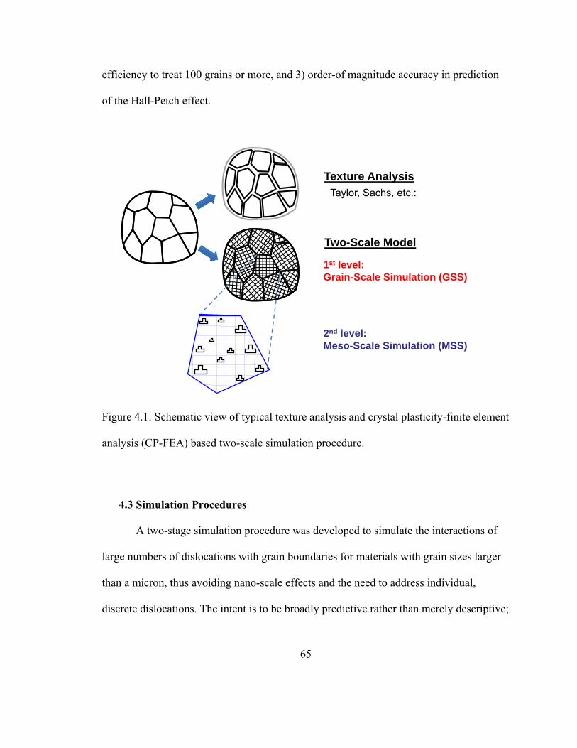
65

efficiency to treat 100 grains or more, and 3) order-of magnitude accuracy in prediction

of the Hall-Petch effect.

2nd

(Dis

Texture Analysis

Two-Scale Model

2nd level: Meso-Scale Simulation (MSS)

1st level: Grain-Scale Simulation (GSS)

Taylor, Sachs, etc.:

Figure 4.1: Schematic view of typical texture analysis and crystal plasticity-finite element

analysis (CP-FEA) based two-scale simulation procedure.

4.3 Simulation Procedures

A two-stage simulation procedure was developed to simulate the interactions of

large numbers of dislocations with grain boundaries for materials with grain sizes larger

than a micron, thus avoiding nano-scale effects and the need to address individual,

discrete dislocations. The intent is to be broadly predictive rather than merely descriptive;

66

therefore the number of undetermined, arbitrary parameters was minimized for the initial

treatment presented here.

The core of the proposed method relies on a standard finite element discretization

of a polycrystal with numerous elements per grain, as shown in Figure 4.1. The Grain-

Scale Simulation (GSS) follows well-established developments appearing in the literature

(Peirce et al., 1983; Asaro and Needleman, 1985; Beaudoin et al., 1994; Sarma and

Dawson, 1996; Dawson et al., 2002; Lee et al., 2009). Mechanical equilibrium is

enforced while maintaining material compatibility in a finite element sense (i.e. at the

nodes). The GSS computes inhomogeneous stress, strain, and slip activity, and, as

inferred from slip magnitudes using established principles, the local generation of

dislocation density on each slip system in each element. (The three constants relating

dislocation density to strain, i.e. strain hardening, are the only undetermined constants in

the formulation. They are readily fit from a measured tensile stress-strain curve.)

The novel Meso-Scale Simulation (MSS) redistributes the mobile dislocation

content for each slip system, as represented by a superdislocation at the center of each

finite element. The mobile part of dislocation density is redistributed in order to

accommodate the plastic strain. The redistribution of mobile dislocation content modifies

the flow stress and back stress in each element according to Orowan’s equation and

elastic inter-dislocation interactions, respectively, which in turn alters the GSS results at

the next time step. Figure 4.2 shows the flow chart of the two-scale modeling scheme.

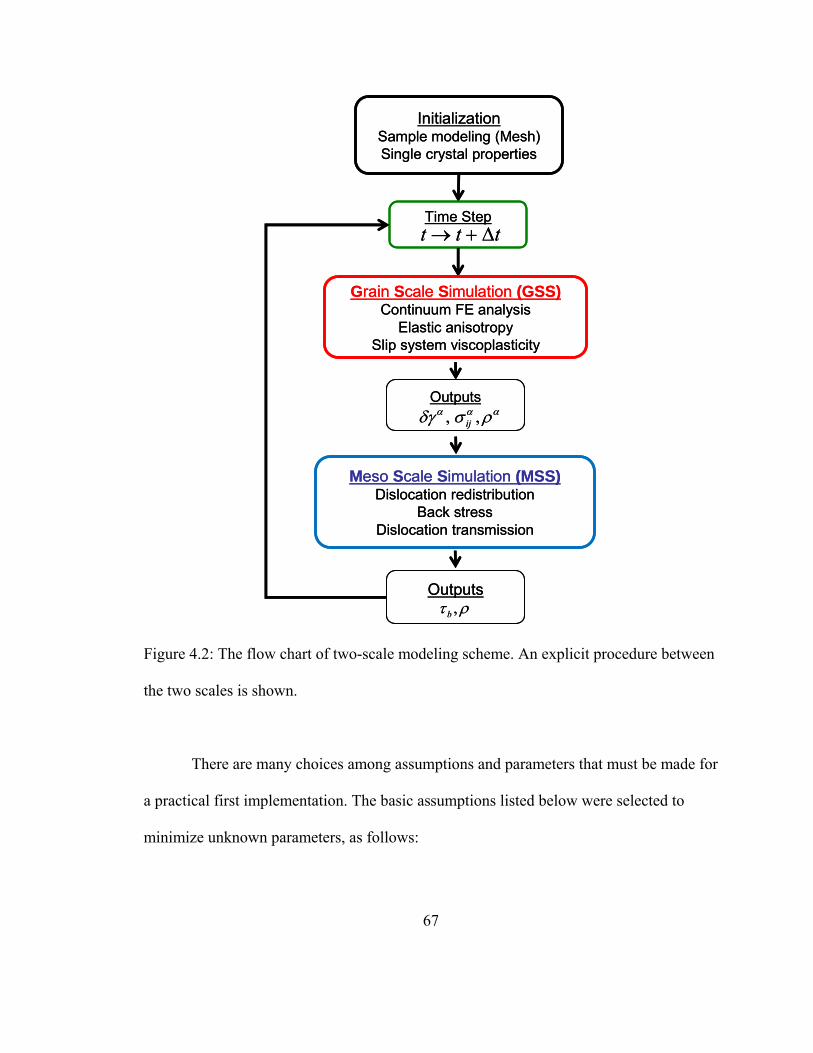
67

InitializationSample modeling (Mesh)Single crystal properties

Time Step

Grain Scale Simulation (GSS)Continuum FE analysis

Elastic anisotropySlip system viscoplasticity

t t t

Outputs

Meso Scale Simulation (MSS)Dislocation redistribution

Back stressDislocation transmission

,b Outputs

, ,ij

InitializationSample modeling (Mesh)Single crystal properties

Time Step

Grain Scale Simulation (GSS)Continuum FE analysis

Elastic anisotropySlip system viscoplasticity

t t t

Outputs

Meso Scale Simulation (MSS)Dislocation redistribution

Back stressDislocation transmission

,b Outputs

, ,ij

Figure 4.2: The flow chart of two-scale modeling scheme. An explicit procedure between

the two scales is shown.

There are many choices among assumptions and parameters that must be made for

a practical first implementation. The basic assumptions listed below were selected to

minimize unknown parameters, as follows:

68

1) All plastic deformation occurs only by slip on fixed slip systems; climb, twinning,

grain boundary sliding, cross-slip and other mechanisms are ignored.

2) The entire dislocation density has edge character such that the line direction is

uniquely determined by slip plane and Burger’s vector.

3) The dislocation density on a single slip system in a finite element can be lumped

into a single superdislocation.

4) For purposes of computing a back stress, dislocations interact only with other

dislocations within the same slip system in a single grain. These interactions are

approximated using isotropic elasticity.

5) Elastic image effects between the dislocation content and the boundaries are

ignored, except as lumped into a grain boundary obstacle stress. The obstacle

stress is the sole effect arising from plastic incompatibility.

4.3.1 Grain-Scale Simulation (GSS)

The GSS procedure follows well-established continuum mechanical principles in

the literature (Lee, 1969; Rice, 1971; Hill and Rice, 1972; Asaro, 1979; Peirce et al.,

1982). It is based on the classical crystal plasticity framework that the total deformation

gradient at a material point within a crystal is described by a multiplicative

decomposition (Lee, 1969).

pFFF e (4.1)

The velocity gradient, pL , is represented in the intermediate configuration in

terms of shear rates as follows (Rice, 1971; Asaro, 1983):

69

1 ( ) ( ) ( )0 0

1

NSp p p

L F F s n

(4.2)

For a strain-rate-dependent crystal model, the crystalline visco-plastic shear rate of the

power-law form defined on the -th slip system may be written as (Hutchinson, 1976;

Peirce et al., 1982):

1

( )( ) ( )

0 ( )sign

m

g

(4.3)

where 0 is a reference shear rate, ( ) and ( )g are the resolved shear stress and the slip

resistance of -th slip system, respectively and m is the rate sensitivity exponent.

Reference shearing rate and rate sensitivity, 0.001 s-1 and 0.012 respectively, were

adopted from the literature (Bronkhorst et al., 1992; Kalidindi et al., 1992).

To this point, the constitutive equations mirror those used routinely for texture

analysis and appearing in the literature. Those standard forms are referred to as the PAN

constitutive model (Peirce, Asaro, Needleman) (Peirce et al., 1982). The evolution of

( )g was formulated using novel single crystal constitutive equations based on

dislocation density herein referred to briefly as SCCE-D (Lee et al., 2009). These

constitutive equations were shown to represent single-crystal behavior accurately for both

FCC and BCC metals (Lee et al., 2009). The remainder of this section outlines the

development of the SCCE-D briefly, with reference to the original publication for details

and testing against measured single crystal behavior and PAN model predictions (Lee et

al., 2009).

70

The dislocation density for SCCE-D in each slip system for each element,

( ) , is computed explicitly. For the first time step, a homogeneous initial dislocation

density, ρ0, corresponding to the yield stress is adopted as using the standard relationship

(Taylor, 1934):

0by (4.4)

where is the shear modulus, b is the Burgers vector, and the parameter is a constant

that depends on the arrangement of dislocations (Widersich, 1964; Olivares and Sevillano,

1987; Schafler et al., 2005). The parameter has been measured and theoretically

calculated for various materials and is generally reported to be in the range 0.3-0.6

(Widersich, 1964; Schoeck and Friedman, 1972; Kassner, 1990; Orlová, 2004; Schafler

et al., 2005; Gubicza et al., 2009). Here, a value of =0.4 was selected as a reasonable

intermediate value. The slip resistance, ( )g , is expressed as follows:

( ) ( )

1

g b h'n

(4.5)

where )( is the dislocation density for slip system , and )(0

)(0αβh ξn

are

interaction cosines where )(0ξ is the dislocation line vector for slip system . To

complete the constitutive equations for a single crystal, a standard phenomenological

model of dislocation evolution is adopted (Kocks, 1976).

71

ba

1k

b k

NS

(4.6)

where, ka and kb are material parameters representing generation and annihilation of

dislocations, respectively. There are thus three fitting parameters for SCCE-D; ρ0, ka

and kb, whereas the conventional PAN model requires four or more adjustable

parameters.

4.3.2 Meso-Scale Simulation (MSS)

The novel MSS utilizes the slip activity and stress computed in each element from

the GSS and redistributes the mobile part of dislocation densities thus changing slip

resistance at the next time step in the GSS. Dislocations interact elastically with the stress

field from the other dislocations and the external stress field. Thus, for n discrete

dislocations interacting, n2 interactions would need to be computed to obtain the

equilibrated spatial distribution of discrete dislocations. A typical range of dislocation

densities is 1010 – 1016 m-2 (Dieter, 1976). It is the size of this problem that puts the direct

treatment of individual dislocation in real materials beyond any realistic estimate

computational abilities.

Discrete dislocations can be treated in a computationally more tractable way by

lumping them within an element to form a superdislocation. A physical pileup of n

discrete dislocations of Burgers vector b can be transformed mathematically into a

statically equivalent one at large distances by lumping the dislocation content within a

72

volume element into a single “superdislocation” with Burgers vector B=nb, where n is

the number of individual dislocation that were lumped. For each slip system type, the

number of interacting superdislocations is equal to the number of finite elements in a

grain (NE). Using this method, the positions of each discrete dislocation is lost, but the

dislocation density within a volume corresponding to the element size is obtained.

A superdislocation for the -th slip system has strength B(), equal to the discrete

dislocation content in that volume on that slip system, as follows:

( ) ( ) ( )( ) ( ) ( )

( )

V bB n b

L

(4.7)

where n() is the number of discrete dislocations of Burgers vector b() on the α-th slip

system and V() and L() are the volume and characteristic length (in the direction parallel

to dislocation line vector) of the element which are stereologically equivalent values for

the slip plane orientation. The characteristic length L() is determined from a line parallel

to the dislocation line passing through the center of the element and terminating at the

element boundaries. The boundaries of the element are readily determined using the

nature of the isoparametric finite elements employed (ABAQUS element C3D8).

The elastic force per unit length operating on the i-th edge superdislocation

segments caused by the stress filed of j-th superdislocation with parallel Burgers vectors

of magnitude B1 and B2 in an isotropic elastic medium is as follows (Hirth and Lothe,

1969):

111 22 12 212 2

2 1 1 2

F 1F

4 (1 ) ( )glide i j

iji

B B rg g g g

dl x x r r

(4.8)

73

where

2,1,)(

)(

222

21

22

21

22

21

22

jixyrrR

rr

rrRx

R

rg

jiij

ijjij

ij

Here, 1r , 2r and 3r are components of position vector ijR as shown in Figure 4.3.

Variables ix and iy denote relative termini of two dislocations in having line direction,

i .

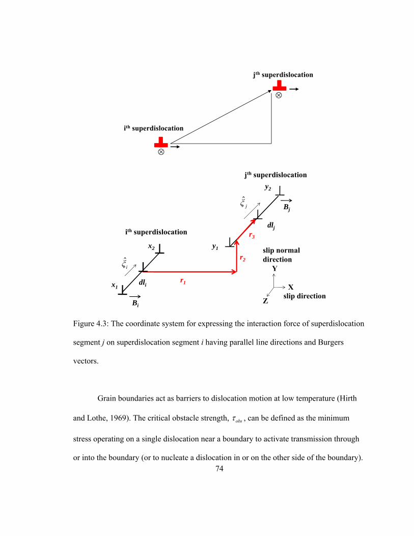
74

ith superdislocation

jth superdislocation

r1

r2

r3

dlj

dli

ith superdislocation

Y

X

Zslip direction

slip normal direction

y2

y1x2

x1

Bi

Bj

jth superdislocation

ˆiξ

ˆjξ

Figure 4.3: The coordinate system for expressing the interaction force of superdislocation

segment j on superdislocation segment i having parallel line directions and Burgers

vectors.

Grain boundaries act as barriers to dislocation motion at low temperature (Hirth

and Lothe, 1969). The critical obstacle strength, obs , can be defined as the minimum

stress operating on a single dislocation near a boundary to activate transmission through

or into the boundary (or to nucleate a dislocation in or on the other side of the boundary).

75

obs may depend on the orientation of the grain boundary (Shen et al., 1986, 1988), the

misorientation of the grains (Livingston and Chalmers, 1957; Shen et al., 1986; De

Messemaeker and Van Humbeek, 2004; Anderson and Shen, 2006), the slip system

geometry and stacking fault energies of the slip plane adjacent to the boundary (Anderson

and Shen, 2006) .

Livingston and Chalmers (Livingston and Chalmers, 1957) first proposed a slip

criterion considering a geometry of slip systems in two adjacent grains and defined slip

transmissivity, N, as follows:

1 1 1 1i i i iN e e g g e g g e (4.9)

where 1e and 1g are the slip plane normal and slip direction of the pileup dislocations in

the incoming plane, and ie and ig are the corresponding quantities in the adjacent grain.

This criterion predicts that dislocations are most easily transmitted through the grain

boundary if the slip transmissivity, N, has a maximum value. This criterion, however,

does not consider the orientation of the grain boundary and failed to predict the emitted

slip systems (Shen et al., 1986).

Shen et al. (Shen et al., 1986) proposed series of alternative slip transmission

criteria (SWC criteria) that consider grain boundary orientations, applied stress or both.

In particular, SWC 2nd criterion (Shen et al., 1986) considers boundary orientation and

predicted emitted slip system relatively well without involving complicated calculation of

local stresses. SWC 2nd criterion is as follows:

1 1( ) ( )i iN L L g g (4.10)

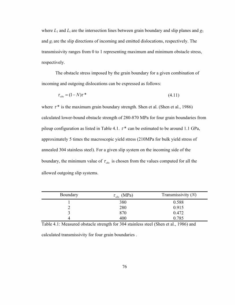
76

where L1 and Li are the intersection lines between grain boundary and slip planes and g1

and gi are the slip directions of incoming and emitted dislocations, respectively. The

transmissivity ranges from 0 to 1 representing maximum and minimum obstacle stress,

respectively.

The obstacle stress imposed by the grain boundary for a given combination of

incoming and outgoing dislocations can be expressed as follows:

(1 ) *obs N (4.11)

where * is the maximum grain boundary strength. Shen et al. (Shen et al., 1986)

calculated lower-bound obstacle strength of 280-870 MPa for four grain boundaries from

pileup configuration as listed in Table 4.1. * can be estimated to be around 1.1 GPa,

approximately 5 times the macroscopic yield stress (210MPa for bulk yield stress of

annealed 304 stainless steel). For a given slip system on the incoming side of the

boundary, the minimum value of obs is chosen from the values computed for all the

allowed outgoing slip systems.

Boundary obs (MPa) Transmissivity (N)

1 380 0.588 2 280 0.915 3 870 0.472 4 400 0.785

Table 4.1: Measured obstacle strength for 304 stainless steel (Shen et al., 1986) and

calculated transmissivity for four grain boundaries .

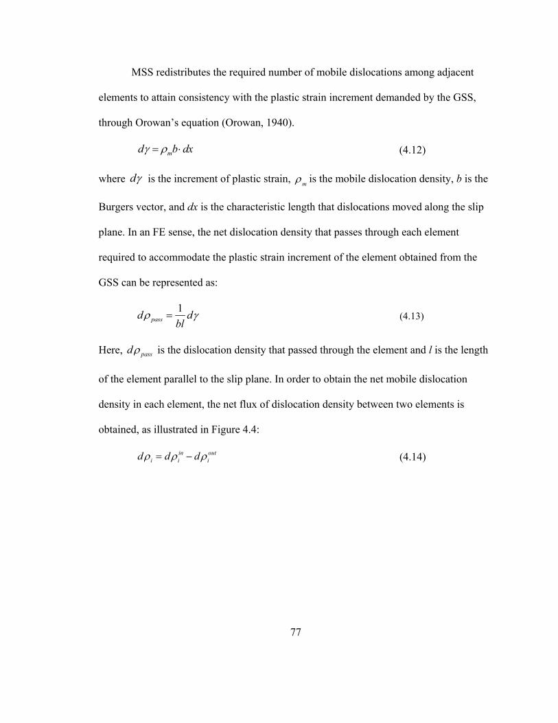
77

MSS redistributes the required number of mobile dislocations among adjacent

elements to attain consistency with the plastic strain increment demanded by the GSS,

through Orowan’s equation (Orowan, 1940).

md b dx (4.12)

where d is the increment of plastic strain, m

is the mobile dislocation density, b is the

Burgers vector, and dx is the characteristic length that dislocations moved along the slip

plane. In an FE sense, the net dislocation density that passes through each element

required to accommodate the plastic strain increment of the element obtained from the

GSS can be represented as:

1passd d

bl

(4.13)

Here, passd is the dislocation density that passed through the element and l is the length

of the element parallel to the slip plane. In order to obtain the net mobile dislocation

density in each element, the net flux of dislocation density between two elements is

obtained, as illustrated in Figure 4.4:

in outi i id d d (4.14)

78

net in outi i id d d

inid out

id

1id id 1id

1il il 1il

netid

1

1( )in i ii

i i

d dd

b l l

1

1( )out i ii

i i

d dd

b l l

Figure 4.4: Redistribution of the mobile dislocation density from one element to adjacent

elements.

After mobile dislocations are redistributed, the back stress is obtained by

considering dislocation interactions within the same slip plane. In contrast to back stress

formulations based on statistical models (Groma, 1997; Yefimov and Van der Giessen,

2004) or strain gradient approaches (Evers et al., 2004), the two-scale model keeps track

of dislocation densities (or, equivalently, the number of dislocations) for each element

and slip system so that the back stress can be obtained explicitly without involving an

arbitrary length scale. The back stress on the i-th dislocation can be represented as

follows:

1

1 Nbi ij

jij i

Fb

(4.15)

The back stress and obstacle strength imposed by the grain boundary are incorporated in

the slip system constitutive response (equation (4.3)) as follows:

For non-grain boundary elements,

79

1/

0 ( )m

effeffsign

g

(4.16)

where ( )beff , and for grain boundary elements,

eff obs

1/

0

'( )

m

eff obseff obssign

g

eff obs 0

(4.17)

(4.18)

where *' (1 )obs N . Note that the obstacle stress is the stress that opposes the slip for

the grain boundary elements and cannot exceed eff . That is, it functions like a frictional

stress and only attains its maximum value when dislocations are being transmitted.

4.3.3 1D stressed pileup

A simple set of parametric test is conducted using the two-scale model to see how

dislocations are redistributed in 1D array of elements upon constant applied stress.

Constant shear stress of 110 MPa is imposed on 1D array of elements (20 solid elements)

with the dimension of 1mm × 20µm × 20µm. Isotropic elasticity is used to calculate the

interaction between dislocations and initial dislocation density is assumed to be zero. One

end of the 1D mesh is assumed to be the grain boundary having * of 375 MPa, while

the other end is regarded as the free surface. For simplicity, only two slip systems are

considered; one that is activated for the slip and the other that only act as forest

dislocations. Constant slip resistance of 10 MPa and reference shear rate of 0.001 s-1 are

adopted. The rate sensitivity exponent, m, is chosen to be 1 to prevent rapid increase of

80

the strain rate. Constant shear stress of 110 MPa to promote the accumulation of

dislocations against the grain boundary is imposed until the tip stress at the head of the

pileup reached the critical obstacle stress. The total number of dislocations within the

specimen was 1.2×104 before the dislocations started to transmit through the grain

boundary.

The identical problem is then solved by using two other methods: (a) analytical

solution based on continuous pileup, and (b) force equilibrium model using finite element

discretization into superdislocations. The analytical solution for the single pileup against

an obstacle by a shear stress is available in Hirth and Lothe (Hirth and Lothe, 1969):

1

22(1 )( )

v l xn x

b x

(4.19)

where is the shear modulus, v is the Poisson’s ratio and b is the Burger’s vector,

respectively. Here, n(x)dx is the number of dislocations between x and x+dx. The pileup

length, l, is obtained from equation (2.6) using the total number of dislocations obtained

from the two-scale model.

Since dislocations experience a net force from other dislocations and applied

stress field, equilibrium requires that the sum of forces on any dislocation is zero. Hence,

using the superdislocation concept, and ignoring lattice friction stresses or other local

constraints to dislocation motion, the defect equilibrium equation condition may be

expressed as follows:

ˆ 0i ij i ij

F F B

(4.20)

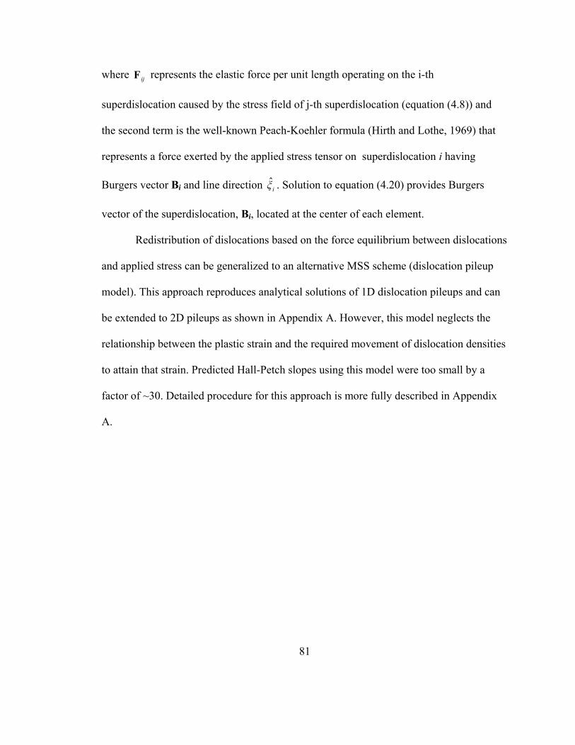
81

where ijF represents the elastic force per unit length operating on the i-th

superdislocation caused by the stress field of j-th superdislocation (equation (4.8)) and

the second term is the well-known Peach-Koehler formula (Hirth and Lothe, 1969) that

represents a force exerted by the applied stress tensor on superdislocation i having

Burgers vector Bi and line direction iξ . Solution to equation (4.20) provides Burgers

vector of the superdislocation, Bi, located at the center of each element.

Redistribution of dislocations based on the force equilibrium between dislocations

and applied stress can be generalized to an alternative MSS scheme (dislocation pileup

model). This approach reproduces analytical solutions of 1D dislocation pileups and can

be extended to 2D pileups as shown in Appendix A. However, this model neglects the

relationship between the plastic strain and the required movement of dislocation densities

to attain that strain. Predicted Hall-Petch slopes using this model were too small by a

factor of ~30. Detailed procedure for this approach is more fully described in Appendix

A.

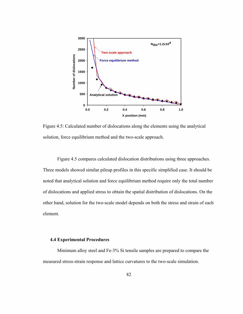
82

X position (mm)

0.0 0.2 0.4 0.6 0.8 1.0

Nu

mb

er o

f d

islo

cati

on

s

0

500

1000

1500

2000

2500

3000

Analytical solution

Two-scale approach

Force equilibrium method

Ndis=1.2x104

Figure 4.5: Calculated number of dislocations along the elements using the analytical

solution, force equilibrium method and the two-scale approach.

Figure 4.5 compares calculated dislocation distributions using three approaches.

Three models showed similar pileup profiles in this specific simplified case. It should be

noted that analytical solution and force equilibrium method require only the total number

of dislocations and applied stress to obtain the spatial distribution of dislocations. On the

other hand, solution for the two-scale model depends on both the stress and strain of each

element.

4.4 Experimental Procedures

Minimum alloy steel and Fe-3% Si tensile samples are prepared to compare the

measured stress-strain response and lattice curvatures to the two-scale simulation.

83

Minimum alloy steel (essentially pure iron with Mn for control of hot shortness) provided

by Severstal N/A has advantages that a wide range of grain sizes is obtainable, it has

good ductility, and, a large Hall-Petch slope was measured as shown in Figure 4.6.

Coarse-grained Fe-3% Si tensile sample which has only single grain through the

thickness is fabricated and provided by AK steel. Material parameters for single crystal

constitutive equations for Fe-3% Si are reasonably well established (Wagoner et al.,

1998) and has an advantage that a wide range of grain sizes, from 10 μm to 30 mm, can

be readily obtained but the sample with grains larger than 2mm showed poor ductility

(<7%). The chemical composition of minimum alloy steel and Fe-3% Si is listed Table

4.2.

D-0.5 (m-0.5)

0 50 100 150 200 250

Yie

ld S

tres

s (

0.2

% o

ffse

t) (

MP

a)

0

100

200

300

400

500

600

0.44 MN/m3/2

0.88 MN/m3/2

0.70 MN/m3/2

Minimum alloy steel

Stainless steel 439

Fe-3% Si

100

D (m)

500 50 30 202000

Figure 4.6: Measured Hall-Petch slope for Fe-3% Si, Stainless steel 439 and minimum

alloy steel.

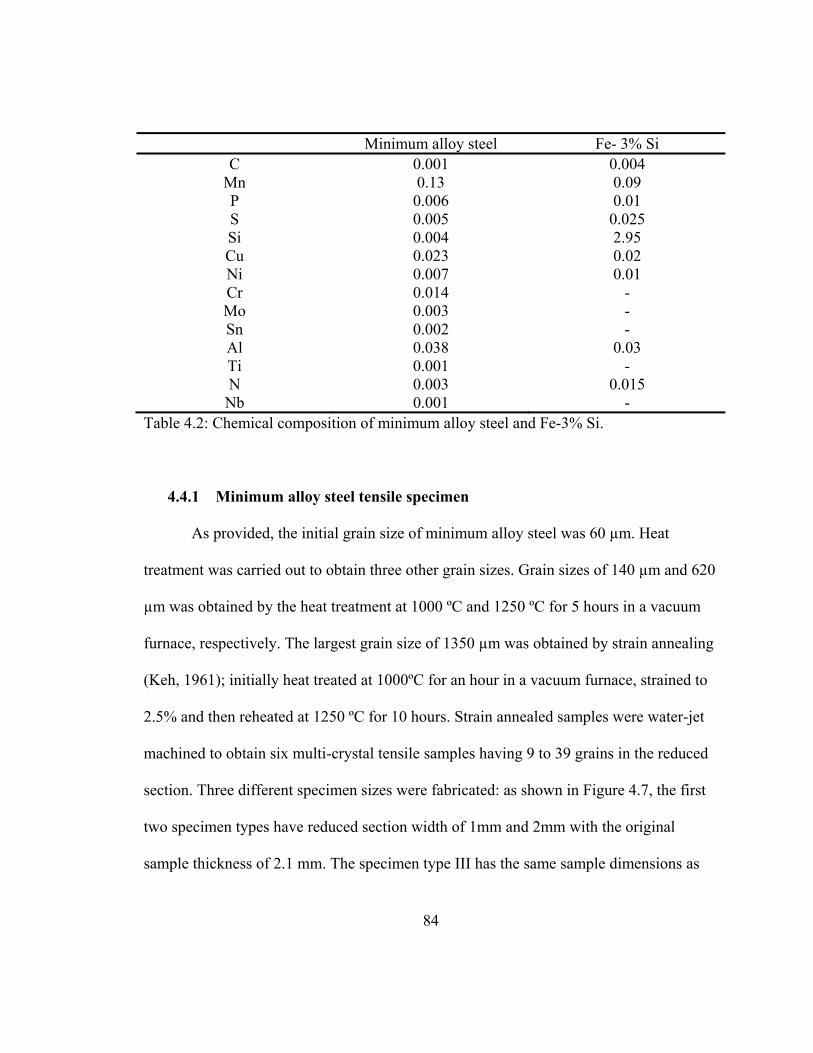
84

Minimum alloy steel Fe- 3% Si C 0.001 0.004

Mn 0.13 0.09 P 0.006 0.01 S 0.005 0.025 Si 0.004 2.95 Cu 0.023 0.02 Ni 0.007 0.01 Cr 0.014 - Mo 0.003 - Sn 0.002 - Al 0.038 0.03 Ti 0.001 - N 0.003 0.015 Nb 0.001 -

Table 4.2: Chemical composition of minimum alloy steel and Fe-3% Si.

4.4.1 Minimum alloy steel tensile specimen

As provided, the initial grain size of minimum alloy steel was 60 µm. Heat

treatment was carried out to obtain three other grain sizes. Grain sizes of 140 µm and 620

µm was obtained by the heat treatment at 1000 ºC and 1250 ºC for 5 hours in a vacuum

furnace, respectively. The largest grain size of 1350 µm was obtained by strain annealing

(Keh, 1961); initially heat treated at 1000ºC for an hour in a vacuum furnace, strained to

2.5% and then reheated at 1250 ºC for 10 hours. Strain annealed samples were water-jet

machined to obtain six multi-crystal tensile samples having 9 to 39 grains in the reduced

section. Three different specimen sizes were fabricated: as shown in Figure 4.7, the first

two specimen types have reduced section width of 1mm and 2mm with the original

sample thickness of 2.1 mm. The specimen type III has the same sample dimensions as

85

type II but rolled in the cold press to obtain the thickness of 0.4 mm (19% of original

thickness).

15.42

60.00

10.00

R16.00

1.00

8.00

15.42

62.00

10.00

R16.00

2.00

10.00

Type I

Type II

Type III

Thickness=2.1 mm

Thickness=2.1 mm

Thickness=0.4 mm

15.42

62.00

10.00

R16.00

2.00

10.00

Sample 1, Sample 2

Sample 3, Sample 6

Sample 4, Sample 5

Figure 4.7: Dimensions of three different tensile sample types for multi-crystal minimum

alloy steel (Unit: mm).

Grain orientations for each sample were then measured using OIM and a FEI-

Philips XL-30 SFEG equipped with a DigiCam system. Figure 4.8 shows grain shapes

within the entire reduced sections of six tensile specimens. Grain orientations

corresponding to the grain numbers indicated in Figure 4.8 are listed in Appendix D.

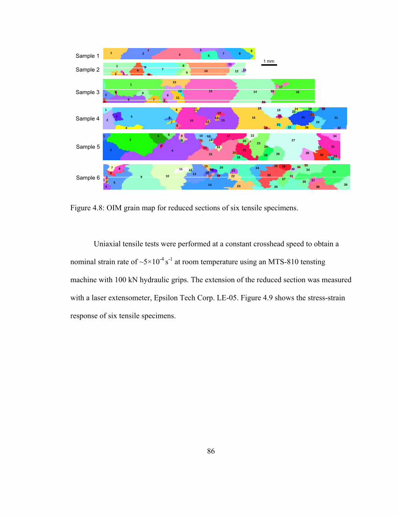
86

1

2

53

6

9

7

4

8

11

1014

13

12

19

18

17

16

15

23

22

21

20

25

24 31

30

29

28

27

26

34

3332

1

2

53

69

7

4

811

10

141312 18

1716

15

1

253 6

97

4

8

1312

1615

14

21

20

19

18

17

26

24

25

22

31

29

28

10

1123

27

30

32

1 2 4

3 58

67

9

1

24

3

5 8

6

79 10

11

12 13

12

53

6

7

4

11

1312 18

1716

15

19

20

10

14

8

9

21

22

23

24

25

26

27

2830

29

31

32 33

34

35

36

37

3839

Sample 1

Sample 2

Sample 3

Sample 4

Sample 5

Sample 6

1 mm

Figure 4.8: OIM grain map for reduced sections of six tensile specimens.

Uniaxial tensile tests were performed at a constant crosshead speed to obtain a

nominal strain rate of ~5×10-4 s-1 at room temperature using an MTS-810 tensting

machine with 100 kN hydraulic grips. The extension of the reduced section was measured

with a laser extensometer, Epsilon Tech Corp. LE-05. Figure 4.9 shows the stress-strain

response of six tensile specimens.

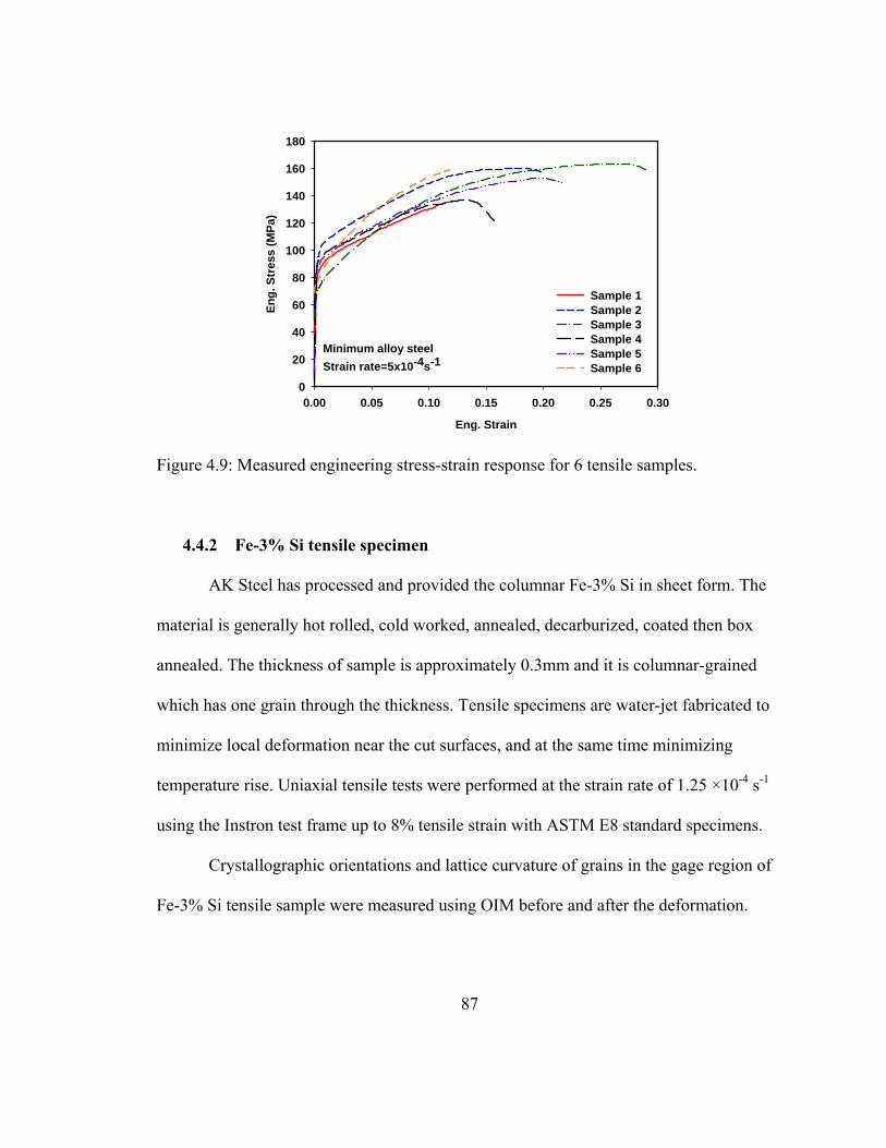
87

Eng. Strain

0.00 0.05 0.10 0.15 0.20 0.25 0.30

En

g. S

tres

s (M

Pa)

0

20

40

60

80

100

120

140

160

180

Sample 1 Sample 2 Sample 3 Sample 4 Sample 5 Sample 6

Minimum alloy steel

Strain rate=5x10-4s-1

Figure 4.9: Measured engineering stress-strain response for 6 tensile samples.

4.4.2 Fe-3% Si tensile specimen

AK Steel has processed and provided the columnar Fe-3% Si in sheet form. The

material is generally hot rolled, cold worked, annealed, decarburized, coated then box

annealed. The thickness of sample is approximately 0.3mm and it is columnar-grained

which has one grain through the thickness. Tensile specimens are water-jet fabricated to

minimize local deformation near the cut surfaces, and at the same time minimizing

temperature rise. Uniaxial tensile tests were performed at the strain rate of 1.25 ×10-4 s-1

using the Instron test frame up to 8% tensile strain with ASTM E8 standard specimens.

Crystallographic orientations and lattice curvature of grains in the gage region of

Fe-3% Si tensile sample were measured using OIM before and after the deformation.

88

The primary objective of OIM analysis is to estimate the small changes in the

orientation of the crystal lattice within the grain of same nominal orientation. This change

has been reported to be associated with the pile-up of dislocation densities near the grain

boundaries. The change in orientation with respect to the change in point of measurement

is described by the lattice curvature tensor, ij (Nye, 1953; Sun et al., 2000).

j

i

dx

d ij

(4.21)

where, id is the change in orientation and jxd is the change in position of the test point.

The diagonal components of ij represent twisting of the lattice about the ix axes, and

the off-diagonal terms represent bending of the ix plane, about the jx direction. Under

the assumption that the mean curvature associated with a specified grain boundary

can be expressed as averaged value of six in-plane components (Adams and Field, 1992;

Sun et al., 2000; El-Dasher et al., 2003).

3

1

2

1

3

1

2

1 6

1

6

1

i j j

i

i jij dx

d

(4.22)

4.5 Results

The two-scale simulation procedure was implemented into ABAQUS/ Standard

(Hibbit, 2005) via user material subroutine UMAT. To assess the accuracy of the

formulation, tensile tests of multicrystal specimens of minimum alloy steel and lattice

curvature of Fe-3% Si alloy with simple two-dimensional columnar structure were

89

simulated and compared with that for the measured. Hardening behavior of multicrystal

minimum alloy steel sample is also predicted using Taylor’s iso-strain model (Taylor,

1938) and conventional PAN constitutive model (Peirce et al., 1982) to be compared with

the two-scale model.

4.5.1 Prediction of Multi-Crystal Stress-Strain Response

The material constitutive response for the two-scale model, PAN model (Peirce et

al., 1982), and Taylor’s iso-strain model adopting SCCE-T and SCCE-D were fit to

reproduce the measured stress-strain response of tensile sample 6, having the most

number of grains (39). Bitmap data for each specimen’s grain map from the OIM

measurements was utilized to distinguish grains and a regular mesh with linear brick

elements (C3D8) was superposed on the image using a total of 8671 elements. The size

of the element was chosen to be smaller than the OIM measurement step size. Detailed

procedures used to obtain the best-fit parameters and the effect of each variable were

described previously (Lee et al., 2009). Anisotropic elasticity constants and shear

modulus for minimum alloy steel used for the simulation are shown in Table 4.3.

µ C11 C12 C44

80 242 150 112 Table 4.3: Shear modulus and anisotropic elasticity constants (Hirth and Lothe, 1969)

(Unit: GPa)

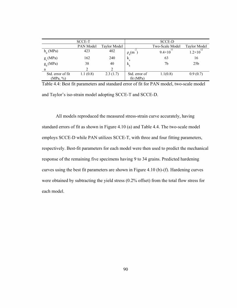
90

SCCE-T SCCE-D PAN Model Taylor Model Two-Scale Model Taylor Model

h0 (MPa) 423 402 ρ

0(m

-2) 9.4×10

11 1.2×10

12

gs (MPa) 162 240 k

a 63 16

g0 (MPa) 38 40 k

b 7b 25b

a 2 2 Std. error of fit

(MPa, %) 1.1 (0.8) 2.3 (1.7) Std. error of

fit (MPa) 1.1(0.8) 0.9 (0.7)

Table 4.4: Best fit parameters and standard error of fit for PAN model, two-scale model

and Taylor’s iso-strain model adopting SCCE-T and SCCE-D.

All models reproduced the measured stress-strain curve accurately, having

standard errors of fit as shown in Figure 4.10 (a) and Table 4.4. The two-scale model

employs SCCE-D while PAN utilizes SCCE-T, with three and four fitting parameters,

respectively. Best-fit parameters for each model were then used to predict the mechanical

response of the remaining five specimens having 9 to 34 grains. Predicted hardening

curves using the best fit parameters are shown in Figure 4.10 (b)-(f). Hardening curves

were obtained by subtracting the yield stress (0.2% offset) from the total flow stress for

each model.

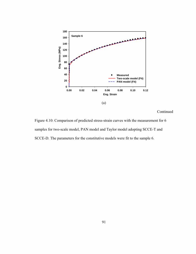
91

0.00 0.02 0.04 0.06 0.08 0.10 0.120

20

40

60

80

100

120

140

160

180

Measured Two-scale model (Fit)PAN model (Fit)

Eng. Strain

En

g. S

tre

ss (

MP

a)

Sample 6

(a)

Continued

Figure 4.10: Comparison of predicted stress-strain curves with the measurement for 6

samples for two-scale model, PAN model and Taylor model adopting SCCE-T and

SCCE-D. The parameters for the constitutive models were fit to the sample 6.

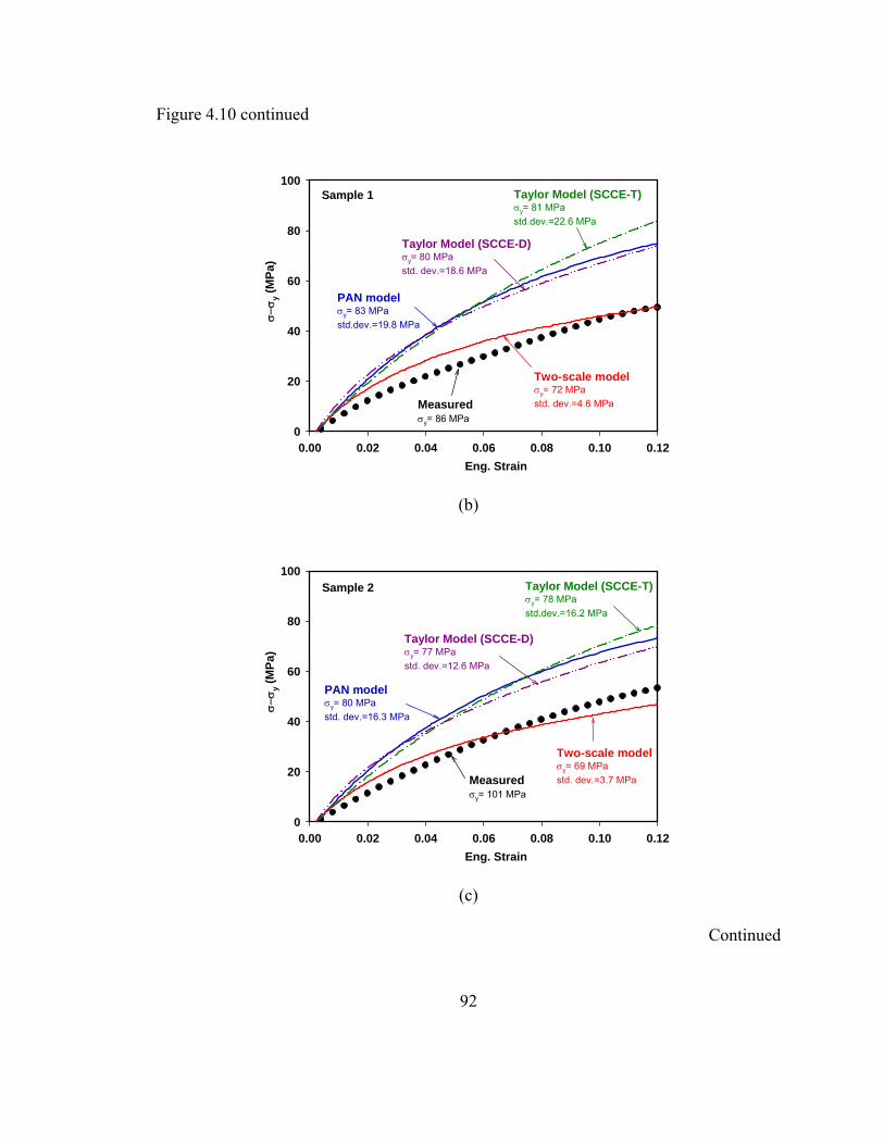
92

Figure 4.10 continued

0.00 0.02 0.04 0.06 0.08 0.10 0.120

20

40

60

80

100

Eng. Strain

y

(M

Pa

)

Sample 1

PAN modely= 83 MPa

std.dev.=19.8 MPa

Two-scale modely= 72 MPa

std. dev.=4.6 MPaMeasuredy= 86 MPa

Taylor Model (SCCE-T)y= 81 MPa

std.dev.=22.6 MPa

Taylor Model (SCCE-D)y= 80 MPa

std. dev.=18.6 MPa

(b)

0.00 0.02 0.04 0.06 0.08 0.10 0.120

20

40

60

80

100

Eng. Strain

y

(M

Pa

)

Sample 2 Taylor Model (SCCE-T)y= 78 MPa

std.dev.=16.2 MPa

Taylor Model (SCCE-D)y= 77 MPa

std. dev.=12.6 MPa

PAN modely= 80 MPa

std. dev.=16.3 MPa

Two-scale modely= 69 MPa

std. dev.=3.7 MPaMeasuredy= 101 MPa

(c)

Continued

93

Figure 4.10 continued

0.00 0.02 0.04 0.06 0.08 0.10 0.120

20

40

60

80

100

Eng. Strain

y

(M

Pa

)

Sample 3 Taylor Model (SCCE-T)y= 76 MPa

std.dev.=6.0 MPaTaylor Model (SCCE-D)y= 75 MPa

std. dev.=18.0 MPa

PAN modely= 81 MPa

std. dev.=6.0 MPa

Two-scale modely= 70 MPa

std. dev.=4.4 MPaMeasuredy= 74 MPa

(d)

0.00 0.02 0.04 0.06 0.08 0.10 0.120

20

40

60

80

100

Eng. Strain

y

(M

Pa

)

Sample 4 Taylor Model (SCCE-T)y= 82 MPa

std.dev.=24.5 MPa

Taylor Model (SCCE-D)y= 80 MPa

std. dev.=8.7 MPa

Two-scale modely= 73 MPa

std. dev.= 4.2 MPaMeasuredy= 95 MPa

PAN modely= 82 MPa

std. dev.= 22.3 MPa

(e)

Continued

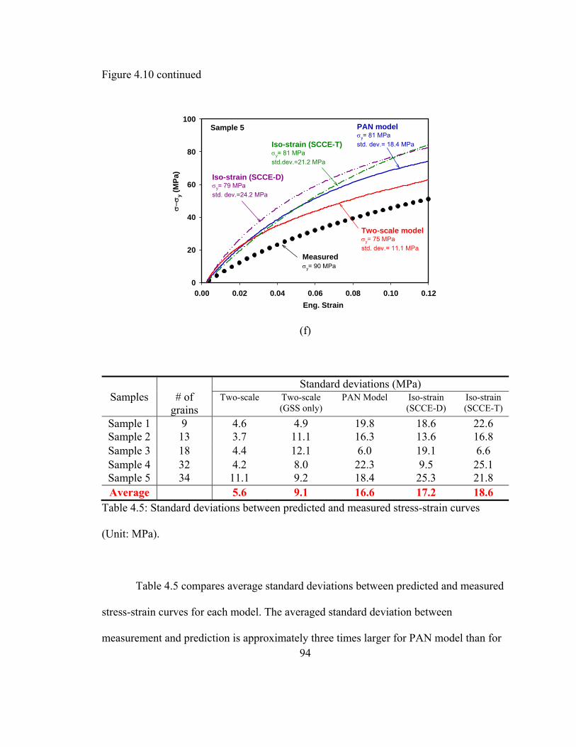
94

Figure 4.10 continued

0.00 0.02 0.04 0.06 0.08 0.10 0.120

20

40

60

80

100

Eng. Strain

y

(M

Pa)

Sample 5

Iso-strain (SCCE-T)y= 81 MPa

std.dev.=21.2 MPa

Iso-strain (SCCE-D)y= 79 MPa

std. dev.=24.2 MPa

PAN modely= 81 MPa

std. dev.= 18.4 MPa

Two-scale modely= 75 MPa

std. dev.= 11.1 MPa

Measuredy= 90 MPa

(f)

Samples

# of

grains

Standard deviations (MPa) Two-scale Two-scale

(GSS only) PAN Model Iso-strain

(SCCE-D) Iso-strain (SCCE-T)

Sample 1 9 4.6 4.9 19.8 18.6 22.6 Sample 2 13 3.7 11.1 16.3 13.6 16.8Sample 3 18 4.4 12.1 6.0 19.1 6.6 Sample 4 32 4.2 8.0 22.3 9.5 25.1 Sample 5 34 11.1 9.2 18.4 25.3 21.8 Average 5.6 9.1 16.6 17.2 18.6

Table 4.5: Standard deviations between predicted and measured stress-strain curves

(Unit: MPa).

Table 4.5 compares average standard deviations between predicted and measured

stress-strain curves for each model. The averaged standard deviation between

measurement and prediction is approximately three times larger for PAN model than for

95

the two-scale model (16.6 MPa vs. 5.6 MPa, respectively). In accordance with similar

tests for single crystals (Lee et al., 2009), the two-scale model adopting SCCE-D agrees

better with measurements compared to the PAN model in spite of having fewer arbitrary

parameters. Taylor models, whether adopting SCCE-T or SCCE-D showed larger

standard deviation compared to two-scale model and PAN model.

The likely source of error for the PAN model and Taylor models lies in ignoring

the role of grain boundaries except as an integral part of the single-crystal constitutive

equation. Figure 4.10 (b)-(f) illustrate that the PAN model tends to over-predict

hardening of the multi-crystals. Recall that all models were fit to multi-crystals with the

most number of grains and the stress-strain response was then predicted for samples with

fewer grains. This over-prediction implies that the best-fit parameters obtained from

Sample 6, which is the most polycrystal-like, do not represent well the hardening

behavior for samples with fewer grains. The averaged standard deviation for prediction

using GSS alone is 9.1 MPa, Table 4.5, larger than the full two-scale model. This

indicates that the back stress and redistribution of mobile dislocations within the MSS

increases accuracy of the prediction over a range of grain configurations.

Despite the two-scale model showing good agreement for hardening of multi-

crystals, both models failed to predict the measured yield stresses accurately using the

current prediction scheme. Values of ρ0 and g0 for SCCE-D and SCCE-T were

determined from the initial yield stress of Sample 6 and the same values. The predicted

yield stresses for the other specimens were 70 to 76 MPa and 81 to 84 MPa for the two-

scale model and PAN model, respectively, while the measured yield stress ranged from

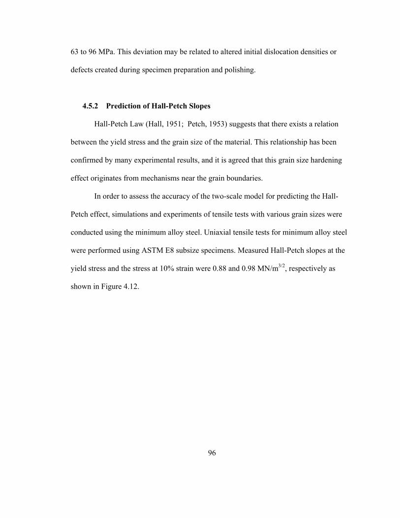
96

63 to 96 MPa. This deviation may be related to altered initial dislocation densities or

defects created during specimen preparation and polishing.

4.5.2 Prediction of Hall-Petch Slopes

Hall-Petch Law (Hall, 1951; Petch, 1953) suggests that there exists a relation

between the yield stress and the grain size of the material. This relationship has been

confirmed by many experimental results, and it is agreed that this grain size hardening

effect originates from mechanisms near the grain boundaries.

In order to assess the accuracy of the two-scale model for predicting the Hall-

Petch effect, simulations and experiments of tensile tests with various grain sizes were

conducted using the minimum alloy steel. Uniaxial tensile tests for minimum alloy steel

were performed using ASTM E8 subsize specimens. Measured Hall-Petch slopes at the

yield stress and the stress at 10% strain were 0.88 and 0.98 MN/m3/2, respectively as

shown in Figure 4.12.

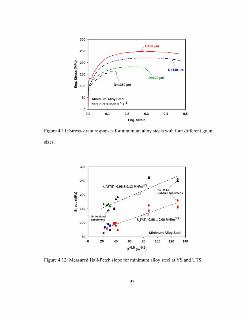
97

Eng. Strain

0.0 0.1 0.2 0.3 0.4 0.5

En

g. S

tres

s (M

Pa)

0

50

100

150

200

250

300

D=1350 m

D=620 m

D=140 m

D=60 m50um

Minimum Alloy Steel

Strain rate =5x10-4 s-1

Figure 4.11: Stress-strain responses for minimum alloy steels with four different grain

sizes.

D-0.5 (m-0.5)

0 20 40 60 80 100 120 140

Str

ess

(MP

a)

50

100

150

200

250

300

ky(UTS)=0.98 0.13 MN/m3/2

ky(YS)=0.88 0.08 MN/m3/2

ASTM E8 Subsize specimens

Undersizedspecimens

Minimum Alloy Steel

Figure 4.12: Measured Hall-Petch slope for minimum alloy steel at YS and UTS.

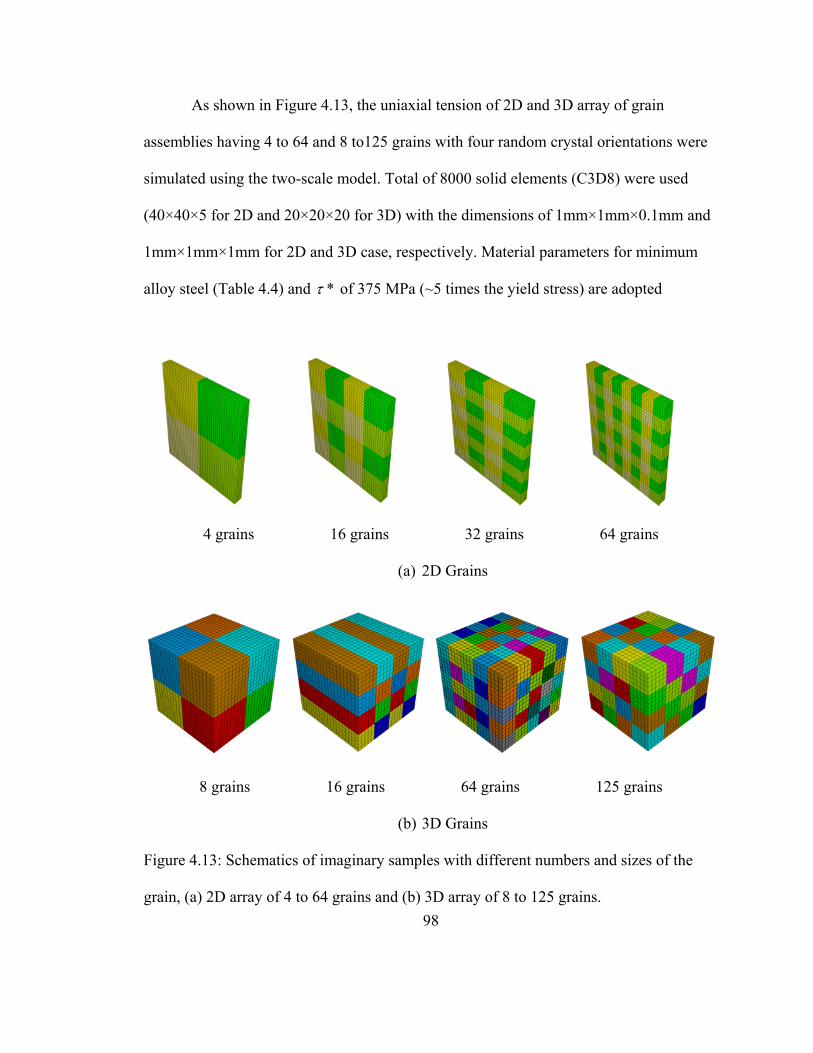
98

As shown in Figure 4.13, the uniaxial tension of 2D and 3D array of grain

assemblies having 4 to 64 and 8 to125 grains with four random crystal orientations were

simulated using the two-scale model. Total of 8000 solid elements (C3D8) were used

(40×40×5 for 2D and 20×20×20 for 3D) with the dimensions of 1mm×1mm×0.1mm and

1mm×1mm×1mm for 2D and 3D case, respectively. Material parameters for minimum

alloy steel (Table 4.4) and * of 375 MPa (~5 times the yield stress) are adopted

4 grains 16 grains 32 grains 64 grains

(a) 2D Grains

8 grains 16 grains 64 grains 125 grains

(b) 3D Grains

Figure 4.13: Schematics of imaginary samples with different numbers and sizes of the

grain, (a) 2D array of 4 to 64 grains and (b) 3D array of 8 to 125 grains.

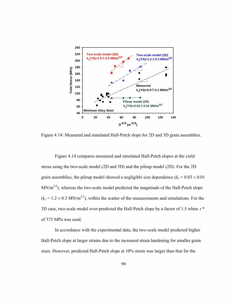
99

D-0.5 (m-0.5)

0 20 40 60 80 100 120 140

Yie

ld S

tres

s (M

Pa)

40

60

80

100

120

140

160

180

200

220

240

Measured

Two-scale model (2D)Two-scale model (3D)

ky(YS)=0.9 0.1 MN/m3/2

Minimum Alloy Steel

ky(YS)=1.2 0.3 MN/m3/2ky(YS)=1.5 0.3 MN/m3/2

Pileup model (2D)ky(YS)=0.03 0.01 MN/m3/2

Figure 4.14: Measured and simulated Hall-Petch slope for 2D and 3D grain assemblies.

Figure 4.14 compares measured and simulated Hall-Petch slopes at the yield

stress using the two-scale model (2D and 3D) and the pileup model (2D). For the 2D

grain assemblies, the pileup model showed a negligible size dependence (ky = 0.03 ± 0.01

MN/m3/2), whereas the two-scale model predicted the magnitude of the Hall-Petch slope

(ky = 1.2 ± 0.3 MN/m3/2), within the scatter of the measurements and simulations. For the

3D case, two-scale model over-predicted the Hall-Petch slope by a factor of 1.5 when *

of 375 MPa was used.

In accordance with the experimental data, the two-scale model predicted higher

Hall-Petch slope at larger strains due to the increased strain hardening for smaller grain

sizes. However, predicted Hall-Petch slope at 10% strain was larger than that for the

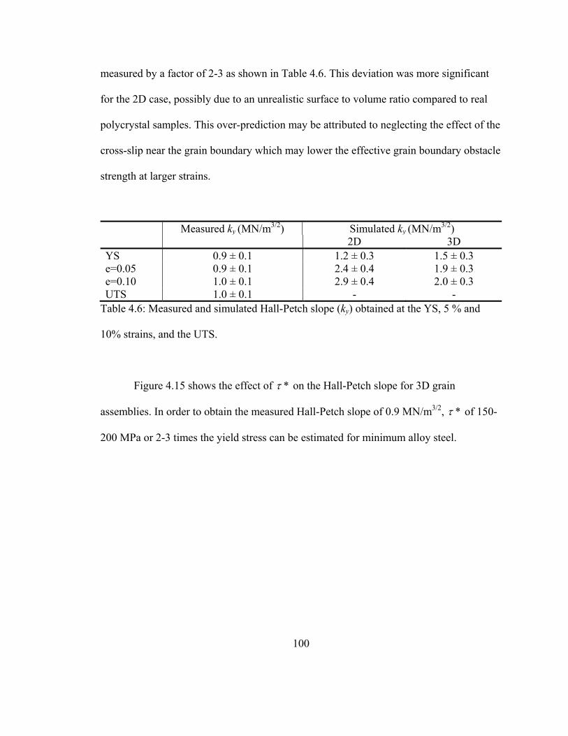
100

measured by a factor of 2-3 as shown in Table 4.6. This deviation was more significant

for the 2D case, possibly due to an unrealistic surface to volume ratio compared to real

polycrystal samples. This over-prediction may be attributed to neglecting the effect of the

cross-slip near the grain boundary which may lower the effective grain boundary obstacle

strength at larger strains.

Measured ky (MN/m3/2) Simulated ky (MN/m3/2) 2D 3D

YS 0.9 ± 0.1 1.2 ± 0.3 1.5 ± 0.3 e=0.05 0.9 ± 0.1 2.4 ± 0.4 1.9 ± 0.3 e=0.10 1.0 ± 0.1 2.9 ± 0.4 2.0 ± 0.3 UTS 1.0 ± 0.1 - -

Table 4.6: Measured and simulated Hall-Petch slope (ky) obtained at the YS, 5 % and

10% strains, and the UTS.

Figure 4.15 shows the effect of * on the Hall-Petch slope for 3D grain

assemblies. In order to obtain the measured Hall-Petch slope of 0.9 MN/m3/2, * of 150-

200 MPa or 2-3 times the yield stress can be estimated for minimum alloy steel.

101

* (MPa)

0 200 400 600

Hal

l-P

etch

Slo

pe,

ky

(MN

/m3

/2)

0.0

0.5

1.0

1.5

2.0

2.5

Measured ky (YS)

Measured ky (e=0.1)

Simulated ky (e=0.1)

Simulated ky (YS)

Figure 4.15: Effect of * on Hall-Petch slope for 3D grain arrays.

4.5.3 Prediction of Lattice Curvature

The initial grain orientations in the gage region of Fe-3% Si tensile specimen are

scanned using the OIM with the step size of 10 µm as shown in Figure 4.16. In order to

measure the lattice curvature with finer OIM step sizes, smaller region of interest with

four grains and two triple junctions is selected (Figure 4.16). The initial Bunge’s Euler

angles for the four grains are listed in Table 4.7. After 8% tensile strain was applied to

the sample, the average lattice curvature is remeasured with 1µm scanning step size.

From the initial grain map, the region of interest is meshed with 9600 elements (C3D8)

and measured stress-strain curve is fitted using the two-scale model, similar to procedure

for minimum alloy steel samples. Best-fit parameters for Fe-3% Si sample are as follows:

ρ0= 7×1012 m-2, ka=98 and kb=8b.

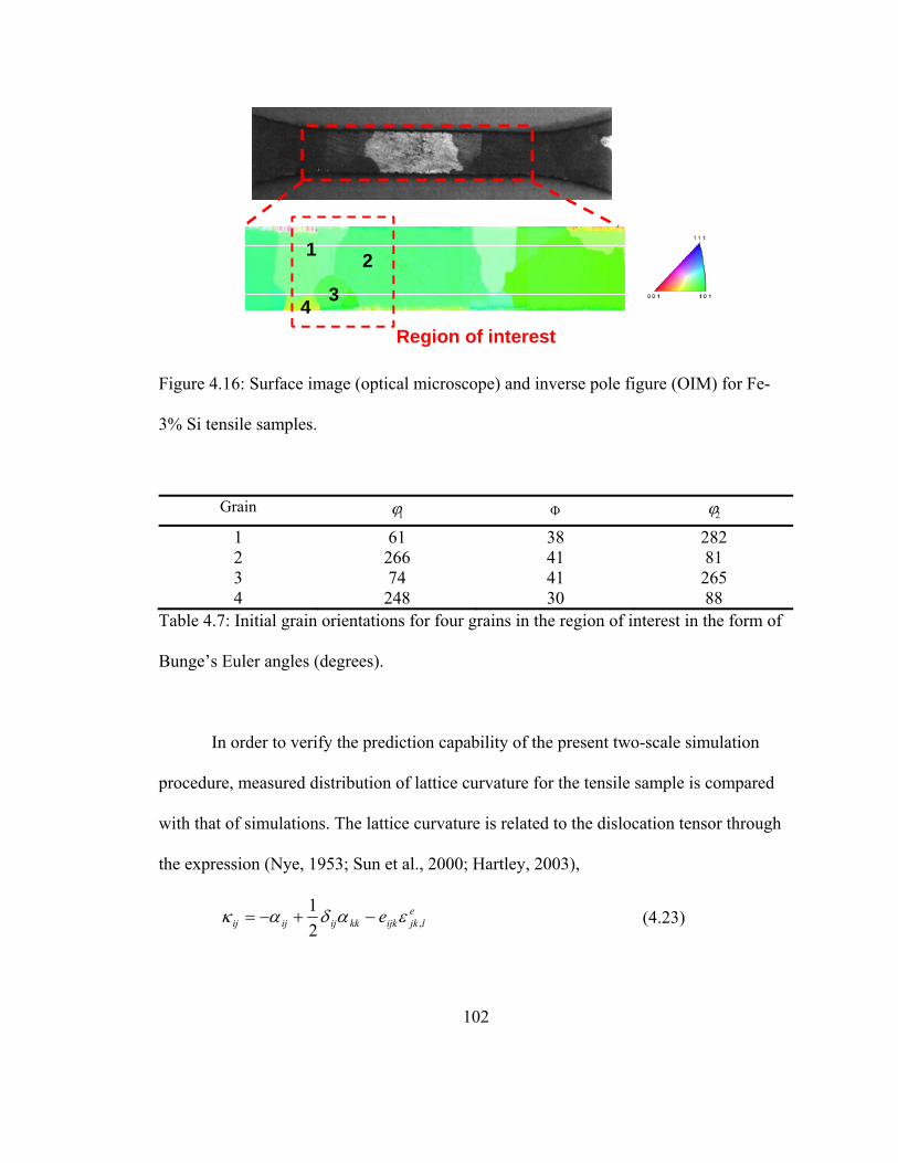
102

Region of interest

12

34

Figure 4.16: Surface image (optical microscope) and inverse pole figure (OIM) for Fe-

3% Si tensile samples.

Grain 1 2

1 61 38 282 2 266 41 81 3 74 41 265 4 248 30 88

Table 4.7: Initial grain orientations for four grains in the region of interest in the form of

Bunge’s Euler angles (degrees).

In order to verify the prediction capability of the present two-scale simulation

procedure, measured distribution of lattice curvature for the tensile sample is compared

with that of simulations. The lattice curvature is related to the dislocation tensor through

the expression (Nye, 1953; Sun et al., 2000; Hartley, 2003),

eljkijkkkijijij e ,2

1

(4.23)

103

where ij is dislocation tensor, ijke denotes components of the permutation tensor. As

shown by Nye (Nye, 1953), there exists a relation between the dislocation tensor and the

network of dislocations as:

NS

s

sss

1

)()()( zbα or

NS

s

sj

si

sij zb

1

)()()( (4.24)

where )(s denotes the density of dislocation type s, b(s) is the Burgers vector of that

type, and z(s) is the line direction of the dislocation type. Since only edge dislocation is

considered in the present two-scale model, the dyadic in equation (4.24) is uniquely

determined with a geometric definition of dislocation on each slip system.

Using equations (4.22), (4.23) and (4.24), the average lattice curvatures are

calculated from the lattice misorientation and dislocation distribution inside the grains.

Figure 4.17 (c)-(e) show the first example of simulated lattice curvature for a Fe-3% Si

specimen after 8% strain. As shown in this figure, high curvatures are developed near the

grain boundaries and near the two triple junctions with predicted curvature distribution

confirmed by the measurements.

Note that high lattice curvatures were measured near the specimen edges due to

surface irregularities. Excluding high lattice curvatures measured near the specimen

edges (dotted line in Figure 4.17 (c)), the difference in maximum magnitude of

curvatures is within 4%: 9.2×10-3 rad/m for the prediction using the two-scale model

and 9.5×10-3 rad/m for the measurement. Two-scale model accurately predicted

maximum lattice curvature and notably low lattice curvature at some grain boundaries, i.e.

the vertical boundary in Figure 4.17 (c). On the other hand, measured averaged lattice

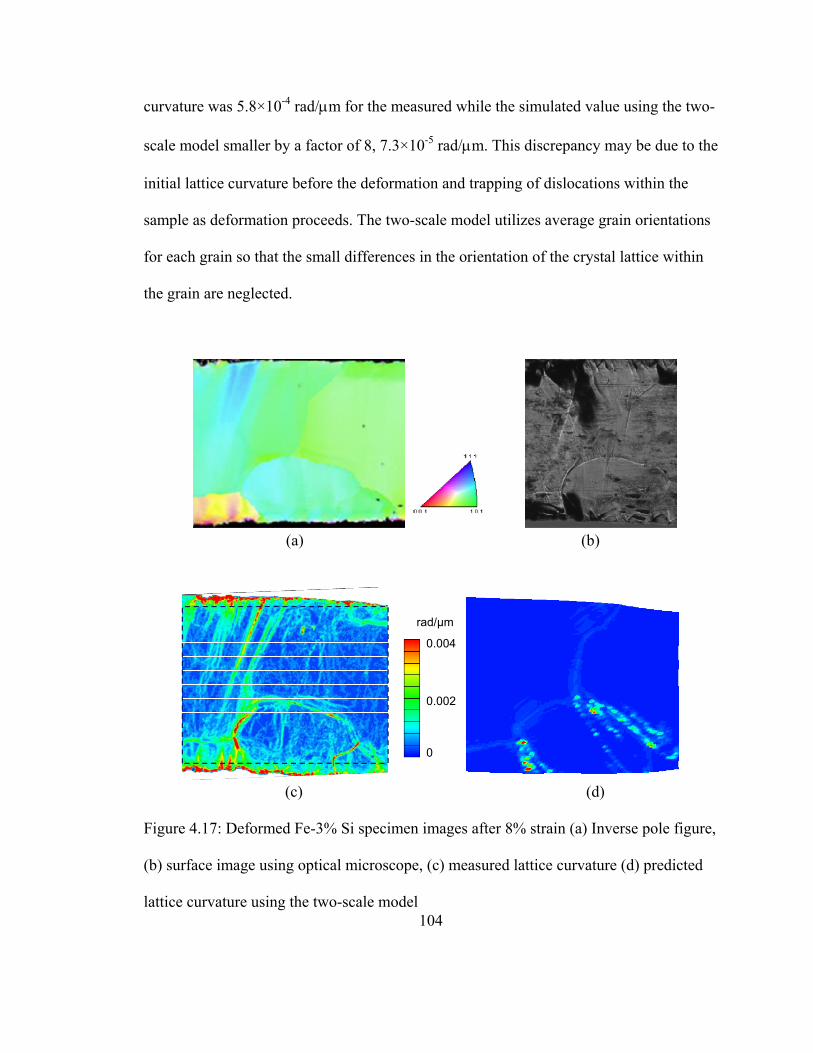
104

curvature was 5.8×10-4 rad/m for the measured while the simulated value using the two-

scale model smaller by a factor of 8, 7.3×10-5 rad/m. This discrepancy may be due to the

initial lattice curvature before the deformation and trapping of dislocations within the

sample as deformation proceeds. The two-scale model utilizes average grain orientations

for each grain so that the small differences in the orientation of the crystal lattice within

the grain are neglected.

(a) (b)

rad/μm

0.004

0.002

0

(c) (d)

Figure 4.17: Deformed Fe-3% Si specimen images after 8% strain (a) Inverse pole figure,

(b) surface image using optical microscope, (c) measured lattice curvature (d) predicted

lattice curvature using the two-scale model

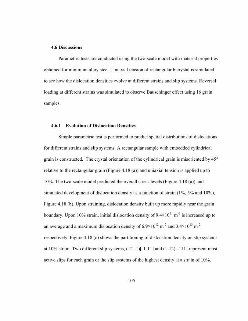
105

4.6 Discussions

Parametric tests are conducted using the two-scale model with material properties

obtained for minimum alloy steel. Uniaxial tension of rectangular bicrystal is simulated

to see how the dislocation densities evolve at different strains and slip systems. Reversal

loading at different strains was simulated to observe Bauschinger effect using 16 grain

samples.

4.6.1 Evolution of Dislocation Densities

Simple parametric test is performed to predict spatial distributions of dislocations

for different strains and slip systems. A rectangular sample with embedded cylindrical

grain is constructed. The crystal orientation of the cylindrical grain is misoriented by 45°

relative to the rectangular grain (Figure 4.18 (a)) and uniaxial tension is applied up to

10%. The two-scale model predicted the overall stress levels (Figure 4.18 (a)) and

simulated development of dislocation density as a function of strain (1%, 5% and 10%),

Figure 4.18 (b). Upon straining, dislocation density built up more rapidly near the grain

boundary. Upon 10% strain, initial dislocation density of 9.4×1011 m-2 is increased up to

an average and a maximum dislocation density of 6.9×1012 m-2 and 3.4×1013 m-2,

respectively. Figure 4.18 (c) shows the partitioning of dislocation density on slip systems

at 10% strain. Two different slip systems, (-21-1)[-1-11] and (1-12)[-111] represent most

active slips for each grain or the slip systems of the highest density at a strain of 10%.

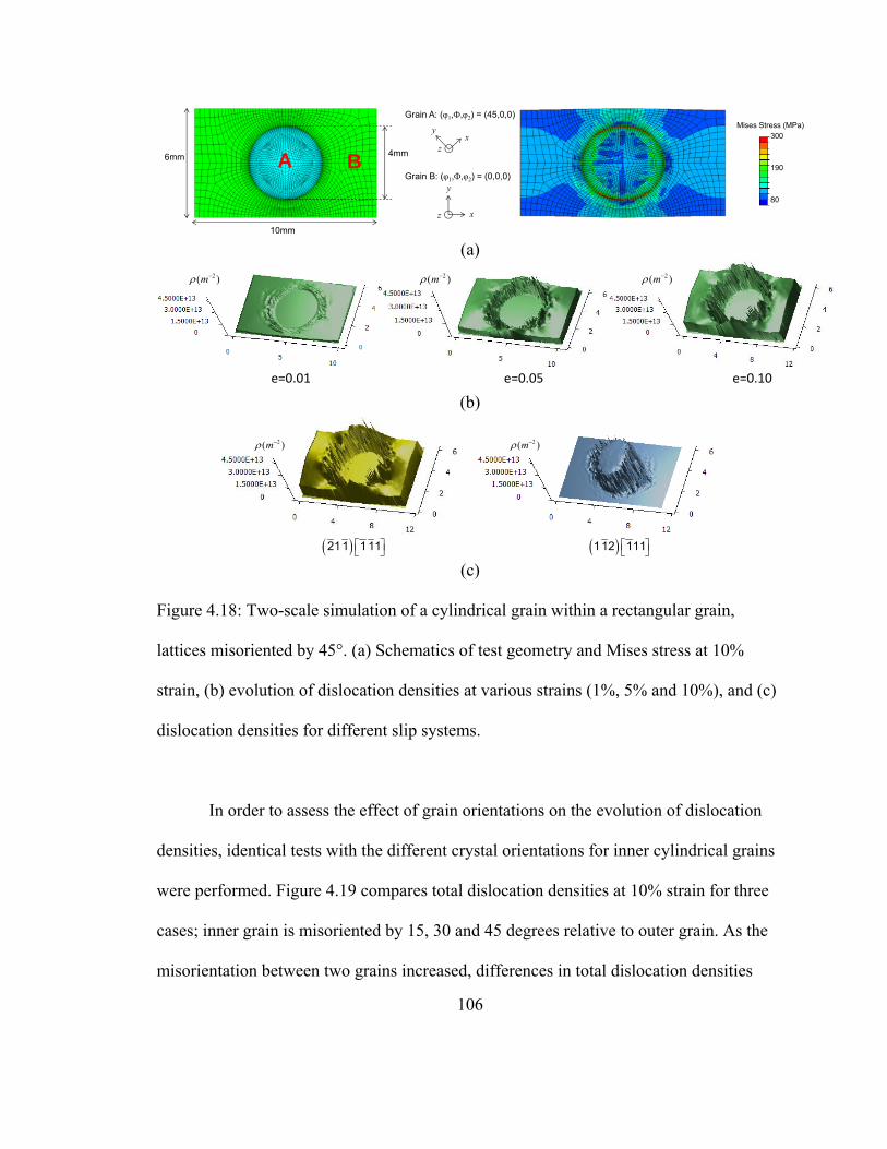
106

6mm

10mm

4mmA By

xz

xy

z

Grain A: (φ1,Ф,φ2) = (45,0,0)

Grain B: (φ1,Ф,φ2) = (0,0,0)

300

80

190

Mises Stress (MPa)

(a) 2( )m 2( )m 2( )m

e=0.01 e=0.05 e=0.10 (b)

2( )m 2( )m

211 111 112 111 (c)

Figure 4.18: Two-scale simulation of a cylindrical grain within a rectangular grain,

lattices misoriented by 45°. (a) Schematics of test geometry and Mises stress at 10%

strain, (b) evolution of dislocation densities at various strains (1%, 5% and 10%), and (c)

dislocation densities for different slip systems.

In order to assess the effect of grain orientations on the evolution of dislocation

densities, identical tests with the different crystal orientations for inner cylindrical grains

were performed. Figure 4.19 compares total dislocation densities at 10% strain for three

cases; inner grain is misoriented by 15, 30 and 45 degrees relative to outer grain. As the

misorientation between two grains increased, differences in total dislocation densities

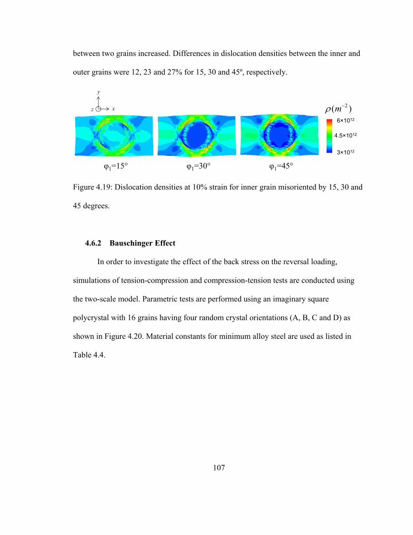
107

between two grains increased. Differences in dislocation densities between the inner and

outer grains were 12, 23 and 27% for 15, 30 and 45º, respectively.

φ1=15° φ1=30° φ1=45°

6×1012

2( )m

4.5×1012

3×1012

y

xz

Figure 4.19: Dislocation densities at 10% strain for inner grain misoriented by 15, 30 and

45 degrees.

4.6.2 Bauschinger Effect

In order to investigate the effect of the back stress on the reversal loading,

simulations of tension-compression and compression-tension tests are conducted using

the two-scale model. Parametric tests are performed using an imaginary square

polycrystal with 16 grains having four random crystal orientations (A, B, C and D) as

shown in Figure 4.20. Material constants for minimum alloy steel are used as listed in

Table 4.4.

108

A B

DC

A B

DC

A B

DC

A B

DCGrain

A 56.66 62.97 185.38

B 130.72 35.24 10.28

C 259.85 25.34 357.48

D 353.88 131.70 271.78

1 2

Figure 4.20: Square polycrystal sample with 16 grains and crystal orientations for each

grain in terms of Bunge’s Euler angles (degrees).

Figure 4.21 (a) and (b) show simulated tension-compression and compression-

tension tests with reversal loadings at 1, 3, and 5% strains. Contrary to most conventional

continuum models, e.g. PAN model, the two-scale model predicted lower yield stress at

the reversal loading due to the back stress. The two-scale model does not require any

fitting parameters to obtain back stress since it is explicitly obtained using interaction

forces among dislocations, equation (4.15) .

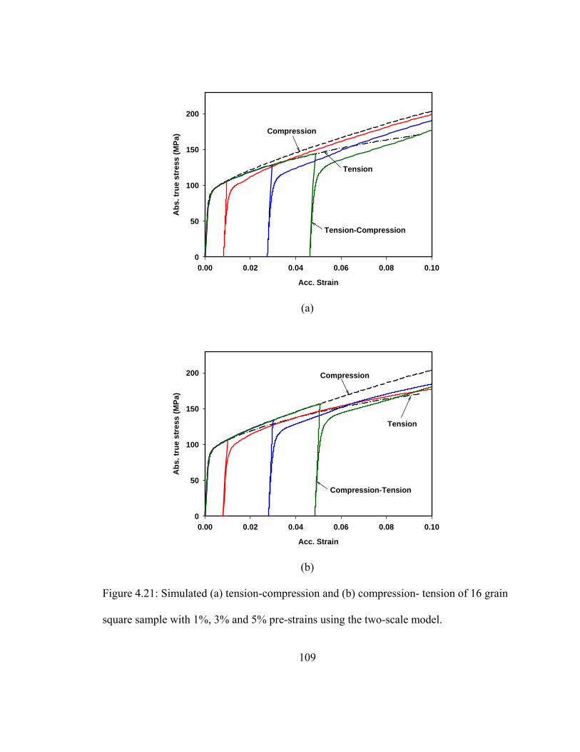
109

Acc. Strain

0.00 0.02 0.04 0.06 0.08 0.10

Ab

s. t

rue

stre

ss (

MP

a)

0

50

100

150

200

Compression

Tension

Tension-Compression

(a)

Acc. Strain

0.00 0.02 0.04 0.06 0.08 0.10

Ab

s. t

rue

stre

ss (

MP

a)

0

50

100

150

200 Compression

Tension

Compression-Tension

(b)

Figure 4.21: Simulated (a) tension-compression and (b) compression- tension of 16 grain

square sample with 1%, 3% and 5% pre-strains using the two-scale model.

110

4.6.3 Efficiency of the Model

The two-scale model was computationally efficient, CPU times required to

simulate 64 grains with 8000 elements was 6.5 hours while that for the pileup model was

13.5 hours. Computational time for the GSS alone was around 6.2 hours so that MSS

contributed only 5% of the total CPU time. Therefore, two-scale model is an efficient and

promising method for treating 100 or more grains.

4.7 Conclusions

A computationally efficient two-scale model was developed capable of predicting

the Hall-Petch effect quantitatively with no arbitrary length scales and only three

arbitrary parameters corresponding to measured strain hardening rates for a single

specimen and grain size. Here are the main conclusions of the work.

1. A two-scale model was developed that is capable of effective and practical

simulation of dislocation densities in polycrystals and their interactions with grain

boundaries based on local boundary/grain properties while reproducing simple

dislocation pile-up solutions. The CPU time to simulate 64 grains with 8000

finite elements deformed to a strain of 10% was 6.5 hours, 95% of which was

used in the standard finite element routine at the larger length scale.

2. The two-scale model accurately predicted the strain hardening of 5 multi-crystal

tensile samples having 9 to 39 grains. Standard texture-type simulations exhibited

standard deviations 3 times greater than those of the two-scale model in spite of

111

having additional undetermined parameters. The average standard deviation

predicted by the two-scale model is 6 MPa as compared with those for the PAN

(Peirce, Asaro, Needleman) / Taylor models with SCCE-D or SCCE-T of 17-19

MPa.

3. PAN and Taylor iso-strain models failed to predict the hardening of multi-crystal

tensile samples accurately. The PAN model was back-fitted from the polycrystal

flow curve (as is usual) and did not adequately represent the behavior of multi-

crystals with fewer numbers of grains. The discrepancy presumably arises from

neglecting the effect of grain boundaries and interaction with dislocations.

4. The two-scale model accurately predicted maximum lattice curvature for a Fe-3%

Si specimen after 8% strain. The maximum lattice curvature predicted by the two-

scale model is 9.5×10-3 rad/m while that for the measured is 9.2×10-3 rad/m,

within 5% deviation.

5. The two-scale model predicted the Hall-Petch effect and its magnitude without

involving related arbitrary parameters. (Only three arbitrary parameters related to

strain hardening were fit, none related to grain size or other lengths scales.) The

simulated Hall-Petch slopes for minimum alloy steel were 1.2 ± 0.3 and 1.5 ± 0.3

MN/m3/2 for 2D and 3D grain assemblies respectively while the corresponding

measured slope was 0.9 ± 0.1 MN/m3/2, approximately within the scatter of the

experiment and simulation.

112

6. Parametric tests showed that if grain boundary strength were treated as an

undetermined parameter, a value 2-3 times the yield stress would match measured

Hall-Petch slopes for minimum alloy steel.

7. Quantitative prediction of spatial distribution of dislocation density has been

carried out and presented. Accumulation of dislocations near grain boundaries

occurs.

113

5. CONCLUSIONS

A computationally efficient two-scale model based on inhomogeneous dislocation

generation, annihilation and accumulation was formulated, implemented and tested

(Chapter 4). In order to implement the two-scale model, a new, more accurate

constitutive model for single crystals was developed (Chapter 3).

1. SCCE-D (the proposed single-crystal constitutive model) reproduces flow curves

for single slip and multi slip in FCC and BCC single crystals. SCCE-D have

better accuracy than SCCE-T (the dominant constitutive model appearing in the

literature) while using a smaller number of adjustable parameters. The average

standard deviation predicted by SCCE-D is 14 MPa while that for the SCCE-T is

31 MPa.

2. SCCE-T, which are usually back-fitted from polycrystal flow curves, do not

adequately represent orientation - dependent single crystal behavior. The

discrepancy may arise from neglecting the effect of grain boundaries, grain size

and relative misorientation between pairs of grains.

3. Polycrystal simulations using SCCE-T fit to multiple-slip single-crystal data

predict higher flow stresses than SCCE-D, correlated with the high flow stresses

predicted by the former for single crystals oriented for limited slip system

114

activation. This correlation implies that there may exist significant regions of

limited slip activation in polycrystals, contrary to the usual assumption.

4. Texture evolution has little sensitivity to the type of constitutive equation.

Simulated textures for SCCE-T and SCCE-D for FCC and BCC polycrystals are

similar, while the simulated macroscopic stress-strain responses differ.

The following conclusions were drawn from the work presented in Chapter 4:

1. A two-scale model was developed that is capable of effective and practical

simulation of dislocation densities in polycrystals and their interactions with grain

boundaries based on local boundary/grain properties while reproducing simple

dislocation pile-up solutions. The CPU time to simulate 64 grains with 8000

finite elements deformed to a strain of 10% was 6.5 hours, 95% of which was

used in the standard finite element routine at the larger length scale.

2. The two-scale model accurately predicted the strain hardening of 5 multi-crystal

tensile samples having 9 to 39 grains. Standard texture-type simulations exhibited

standard deviations 3 times greater than those of the two-scale model in spite of

having additional undetermined parameters. The average standard deviation

predicted by the two-scale model is 6 MPa as compared with those for the PAN

(Peirce, Asaro, Needleman) / Taylor models with SCCE-D or SCCE-T of 17-19

MPa.

3. PAN and Taylor iso-strain models failed to predict the hardening of multi-crystal

tensile samples accurately. The PAN model was back-fitted from the polycrystal

115

flow curve (as is usual) and did not adequately represent the behavior of multi-

crystals with fewer numbers of grains. The discrepancy presumably arises from

neglecting the effect of grain boundaries and interaction with dislocations.

4. The two-scale model accurately predicted maximum lattice curvature for a Fe-3%

Si specimen after 8% strain. The maximum lattice curvature predicted by the two-

scale model is 9.5×10-3 rad/m while that for the measured is 9.2×10-3 rad/m,

within 5% deviation.

5. The two-scale model predicted the Hall-Petch effect and its magnitude without

involving related arbitrary parameters. (Only three arbitrary parameters related to

strain hardening were fit, none related to grain size or other lengths scales.) The

simulated Hall-Petch slopes for minimum alloy steel were 1.2 ± 0.3 and 1.5 ± 0.3

MN/m3/2 for 2D and 3D grain assemblies respectively while the corresponding

measured slope was 0.9 ± 0.1 MN/m3/2, approximately within the scatter of the

experiment and simulation.

6. Parametric tests showed that if grain boundary strength were treated as an

undetermined parameter, a value 2-3 times the yield stress would match measured

Hall-Petch slopes for minimum alloy steel.

7. Quantitative prediction of spatial distribution of dislocation density has been

carried out and presented. Accumulation of dislocations near grain boundaries

occurs.

116

6. REFERENCES

Abson, D. J., Jonas, J. J. (1970). "Hall-Petch relation and high-temperature subgrains."

Metal. Sci. J. 4: 24-28.

Acharya, A. (2001). "A model of crystal plasticity based on the theory of continuously

distributed dislocations." J. Mech. Phys. Solids(49): 761.

Adams, B. L., Field, D. P. (1992). "Measurement and representation of grain boundary

texture." Metall. Trans A(23A): 2501.

Alcalá, J., Casals, O., Očenášek, J. (2008). "Micromechanics of pyramidal indentation in

fcc metals: Single crystal plasticity finite element analysis." J. Mech. Phys. Solids

56: 3277-3303.

Anand, L., Gurland, J. (1976). "Effect of internal boundaries on the yield strengths of

spheroidized steels." Met. Trans. A 7A: 191.

Anand, L., Kothari, M. (1996). "A computational procedure for rate-independent crystal

plsticity." J. Mech. Phys. Solids 44: 525.

Anderson, P. M., Shen, Y. (2006). "Transmission of a screw dislocation across a coherent,

slipping interface." Acta. Mater. 54: 3941-3951.

Armstrong, R. W. (1970). "Influence of polycrystal grain size on mechanical properties."

Adv. Mater. Res. 4: 101-145.

117

Arsenlis, A., Parks, D. M. (2002). "Modeling the evolution of crystallographic

dislocation density in crystal plasticity." J. Mech. Phys. Solids 5-: 1979.

Arsenlis, A., Parks, D. M., Becker, R., Bulatov, V. V. (2004). "On the evolution of

crystallographic dislocation density in non-homogeneously deforming crystals." J.

Mech. Phys. Solids(52): 1213.

Asaro, R. J. (1979). Acta. Met. 27: 445.

Asaro, R. J. (1983). "Micromechanics of crystals and polycrystals." Adv. Appl. Mech.

23: 1-115.

Asaro, R. J., Needleman, A. (1985). "Texture development and strain hardening in rate

dependent polycrystals." Acta metall. 33: 923-953.

Asaro, R. J., Rice, J. R (1977). "Strain localization in ductile single crystals." J. Mech.

Phys. Solids 25: 309-338.

Ashby, M. F. (1970). "Mechancial effects of a dispersion of a second phase." Phil. Mag.

21: 399.

Baldwin, W. M. (1958). Acta Mater. 11: 75.

Bassani, J. L., Wu, T. Y. (1991). "Latent hardening in single crystals ii. Analytical

characterization and predictions." Proc. R. Soc. London A 435: 21.

Beaudoin, A. J., Dawson, P. R., Mathur, K. K., Kocks, U. F., Korzekwa, D. A. (1994).

"Application of polycrystal plasticity to sheet forming." Computer methods in

applied mechanics and engineering 117: 49-70.

Becker, R., Panchanadeeswaran, S. (1995). "Effects of grain interactions on deformation

and local texture in polycrystals." Acta Metall. Mater. 43: 2701.

118

Bergström, Y. (1970). "Dislocation model for the stress-strain behaviour of

polycrystalline alpha-iron with special emphasis on the variation of the densities

of mobile and immobile dislocations." Mat. Sci. Eng. 5(4): 193-200.

Bergström, Y., Hallen, H. (1982). "An improved dislocation model for the stress-strain

behaviour of polycrystalline a-Fe." Mat Sci Eng 55: 49-61.

Bernstein, I. M., Rath, B. B. (1973). "Role of grain boundary solutes and structure on the

yielding and intergranular cracking of Fe." Met. Trans. 4(6): 1545-1551.

Biner, S. B., Morris, J. R. (2003). "The effects of grain size and dislocation source

density on the strengthening behaviour of polycrystals: a two dimensional discrete

dislocation simulation." Phil. Mag. 83: 3677-3690.

Bronkhorst, C. A., Kalidinidi, S. R., Anand, L. (1992). "Polycrystalline plasticity and the

evolution of crystallographic texture in FCC metals." Philos. Trans. Roy. Soc.

London A 341(443).

Brown, L. M., Kim, K. H., Anand, L. (1989). "An internal variable constitutive model for

hot working of metals." Int. J. Plasticity 5: 95-130.

Budiansky, B., Wu, T. T. (1962). Theoretical prediction of plastic strains of polycrystals. .

Procd. 4th U. S. Nat. Cong. of Applied Mech.

Bunge, H. J. (1965). "Zur darstellung allgemeiner texturen." Z. Metallk.(56): 872.

Canova, G. R., Kocks, U. F., Tome, C. N., Jonas, J. J. (1985). "The yield surface of

textured polycrystals." J. Mech. Phys. Solids 33: 371-397.

119

Chang, P. H., Preban, A. G. (1985). "The effect of ferrite grain size and martensite

volume fraction on the tensile properties of dual phase steel." Acta metall. 33(5):

897-903.

Chia, K., Jung, K., Conrad, H. (2005). "Dislocation density model for the effect of grain

size on the flow stress of a Ti-15.2 at.% Mo b-alloy at 4.2-650K." Mater. Sci.

Eng.A 409: 32-38.

Chokshi, A. H., Rosen, A., Karch, J., Gleiter, H. (1989). "On the validity of the Hall-

Petch relationship in nanocrystalline materials." Scripta. Met. 23: 1679-1684.

Chou, Y. T. (1967). "Dislocation Pileups Against a Locked Dislocation of a Different

Burgers Vector." J. Appl. Phys. 38: 2080-2085.

Christman, T. (1993). "Grain Boundary Strengthening Exponent in Conventional and

Ultrafine Microstructures." Scr. Metall. Mater. 28(12): 1495-1500.

Clark, W. A. T., Wagoner, R. H., Shen, Z. Y. (1992). "On the criteria for slip

transmission across interfaces in polycrystals." Scripta. Met. et Mater 26: 203-206.

Conrad, H. (1961). Electron Microscopy and Strength of Crystals, Interscience, New

York.

Conrad, H. (1970). Ultrafine-Grain Metals, Syracuse University Press, Syracuse, New

York.

Conrad, H. (2004). "Grain-size dependence of the flow stress of Cu from millimeters to

nanometers." Metall. Mat. Trans. A 35A: 2681-2695.

Conrad, H., Feuerstein, S., Rice, L (1968). Trans. Japan Inst. Metals 9: 481.

120

Cottrell, A. H. (1953). Dislocations and plastic flow in crystals, Oxford University Press,

London.

Cottrell, A. H. (1958). "Theory of brittle fracture in steel and similar metals." Trans.

Metall. Soc. AIME. 212: 192-203.

Cuitiño, A. M., Ortiz, M. (1992). "Computational modeling of single crystals." Model.

Simul. Mater. Sci. Eng. 1: 225.

Dawson, P. R. (2000). "Computational crystal plasticity." International Journal of Solids

and Structures 37: 115-130.

Dawson, P. R., MacEwen, S. R., Wu, P. D. (2003). "Advances in sheet metal forming

analyses, dealing with mechanical anisotropy from crystallographic texture." Int.

Mater. Rev. 48 (2): 86-122.

Dawson, P. R., Mika, D.P., Barton, N.R. (2002). "Finite element modeling of lattice

misorientations in aluminum polycrystals." Scripta Mater 47(10): 713-717.

De Messemaeker, J. V., B., Van Humbeek, J. (2004). "On the strength of boundaries in

submicrom IF steel." Materials Letters 58: 3782-3786.

Dieter, G. E. (1976). Mechanical Metallurgy. McGraw Hill, Second Edition.

Domkin, K., Lindgren, L., Segle, P. (2003). Dislocation density based models for plastic

hardening and parameter identification. 7th International Conference on

Computational Plasticity, COMPLA2003, Barcelona.

El-Dasher, B. S., Adams, B. L., Rollett, A. D. (2003). "Viewpoint: Experimental

recovery of geometrically necesary dislocation density in polycrystals." Scripta

Mater(48): 141.

121

Eshelby, J. D. (1957). The determination of the elastic field of an ellipsoidal inclusion,

and related problems. Proc. R. Soc. Lond.

Essmann, U., Mughrabi, H. (1979). "Annihilation of dislocations during tensile and

cyclic deformation and limits of dislocation densities." Phil. Mag. A40: 731.

Estrin, Y. (1998). "Dislocation theory based constitutive modelling: foundations and

applications." Journal of Materials Processing Technology 80-81: 33-39.

Estrin, Y., Mecking, H. (1984). "A unified phenomenological description of work

hardening and creep based on one-parameter model." Acta metall. 32(1): 57-70.

Evans, J. W., Rawlings, R. D. (1969). Mater Sci Eng A 4: 197.

Evans, P. R. V. (1963). "The dependence of the lower yield stress on grain size in

niobium." J. Inst. Metals 92: 57.

Evers, L. P., Brekelmans, W. A. M., Geers, M. G. D. (2004). "Non-local crystal plasticity

model with intrinsic SSD and GND effects." J. Mech. Phys. Solids 52: 2379-2401.

Evers, L. P., Parks, D. M., Brekelmans, W. A. M., Geers, M. G. D. (2002). "Crystal

plasticity model with enhanced hardening by geometrically necessary dislocation

accumulation." J. Mech. Phys. Solids 50(11): 2403-2424.

Fang, L., Friedman, L. H. (2007). "Analytical treatment of metallic multilayer strength at

all length scales: Influence of dislocation sources." Acta Mater. 55: 1504-1514.

Feaugas, X., Haddou, H (1999). "On the origin of the tensile flow stress in the stainless

steel AISI 316L at 300K: back stress and effective stress." Acta Mater. 47: 3617.

Feaugas, X., Haddou, H (2003). "Grain-size effects on tensile behavior of nicke and AISI

316L strainless steel." Met. Trans. A 34: 2329.

122

Fleck, N. A., Hutchinson, J. W. (1997). "Strain gradient plasticity." Adv. Appl.

Mech.(33): 295.

Fleck, N. A., Muller, G. M., Ashby, M. F., Hutchinson, J. W. (1994). "Strain gradient

plasticity, theory and experiment." Acta Metall. Mater.(42): 475.

Floreen, S., Westbrook, J. H. (1969). "Grain-boundary segregation and the grain-size

dependence of strength of nickel-sulphur alloys." Acta Metall. 17(9): 1175-1181.

Follansbee, P. S., Kocks, U. F. (1988). "A constitutive description of the deformation of

copper based on the use of the mechanical threshold stress as an internal state

variable." Acta Metall. Mater.(36): 81.

Franciosi, P., Zaoui, A. (1982). "Multislip in F.C.C crystals: a theoretical approach

compared with experimental data." Acta Metall. 30: 1627.

Gottstein, G., Argon, A. S. (1987). "Dislocation theory of steady state deformation and its

approach in creep and dynamic tests." Acta Metal. 92(1-2): 1261-1271.

Grabski, M. W. W., J W (1980). "The Effect of the Spreading of Grain Boundary

Dislocations on the Tensile Behavior of a Fine-Grained Austenitic Steel at High

Temperatures." Mater. Sci. Eng. 44(2): 229-237.

Gray, I. G. T., Chen, S. R., Vecchio, K. S. (1999). "Influence of grain size on the

constitutive response and substructure evolution of MONEL 400." Metall. Mat.

Trans. A 30: 1235.

Groma, I. (1997). "Link between the microscopic and mesoscopic length-scale

description of the collective behavior of dislocations." Physical Review B. 56(10):

5807-5813.

123

Gubicza, J., Chinh, N. Q., Lábár, J. L., Dobatkin, S., Hegedüs, Z., Langdon, T. G. (2009).

"Correlation between microstructure and mechanical properties of severely

deformed metals." Journal of Alloys and Compounds 483: 271-274.

Gurtin, M. E. (2000). "On the plasticity of single crystals, free energy, microforces,

plastic strain gradients." J. Mech. Phys. Solids(48): 989.

Gurtin, M. E. (2002). "A gradient theory of single-crystal viscoplasticity that accounts for

geometrically necessary dislocations." J. Mech. Phys. Solids(50): 5.

Haasen, P. (1989). "A Cell Theory for Stage IV Work Hardening of Metals and

Semiconductors." J. Phys. France 50(18): 2445-2453.

Hall, E. O. (1951). "The deformation and ageing of mild steel." Proc. Roy. Soc. (London)

B64: 747.

Hall, E. O. (1970). Yield point phenomena in metals and alloys. New York, Plenum Press.

Hartley, C. S. (2003). "A method for linking thermally activated dislocation mechanisms

of yielding with contiuum plasticity theory." Phil. Mag.(83): 3783.

Hibbit, K. S. I. (2005). ABAQUS/Standard User's Manual.

Hill, R. (1966). "Generallized constitutive relations for incremental deformation of metal

crystals by multislip." J. Mech. Phys. Solids 14(95).

Hill, R., Rice, J.R. (1972). "Constitutive analysis of elastic plastic crystals at arbitrary

strain." J. Mech. Phys. Solids 20(401).

Hirth, J. P. (1972). "Influence of grain boundaries on mechancal properties." Met. Trans.

3: 3047.

124

Hirth, J. P. (2006). "Dislocation pileups in the presence of stress gradients." Philos. Mag.

86 (25,26): 3959-3963.

Hirth, J. P., Lothe, J. (1969). Theory of Dislocations, McGraw-Hill, New York.

Honneff, H. (1978). Analysis of the deformation texture at different rolling conditions,

Berlin: Springer-Verlag.

Hook, R. E., Hirth, J. P. (1967). "The deformation behavior of isoaxial bicrystals of Fe-

3% Si." Acta Metal.(15): 535.

Hull, D. (1975). "Effect of grain size and temperature on slip twinning and fracture in 3%

silicon iron." Acta. Met. 9(191).

Hutchinson, J. W. (1970). "Elastic-plastic behaviour of polycrystalline metals and

composites." Proc. Roy. Soc. London A319: 247-272.

Hutchinson, J. W. (1976). Bounds and self-consistent estimates for creep of

polycrystalline materials. Proc. R. Soc. London.

Jago, R. A., Hansen, N. (1986). "Grain size effects in the deformation of polycrystalline

iron." Acta metall. 34(9): 171101720.

Kako, K., Kawakami, E., Ohta, J., Mayuzumi, M (2002). "Effect of various alloying

elements on tensile properties of high purity Fe-18Cr-(14-16) Ni alloys at room

temperature." Materials transactions 43(2): 155-162.

Kalidindi, S. R., Bronkshorst, C. A., Anand, L. J. (1992). "Crystallographic texture

evolution in bulk deformation processing of FCC metals." J. Mech. Phys. Solids

40(537).

125

Kassner, M. E. (1990). "A case for Taylor hardening during primary and steady-state

creep in aluminium and type 304 stainless steel." J. Mater. Science. 25: 1997-

2003.

Keh, A. S. (1961). Electron Microscopy and Strength of Crystals, Interscience, New York

Keh, A. S. (1965). "Work hardening and deformation sub-structure in iron single crystals

deformed in tension at 298K." Phil. Mag. 12: 9.

Kocks, U. F. (1959). Acta metall. 7: 131.

Kocks, U. F. (1970). "The relation between polycrystal deformation and single crystal

deformation." Metall. Trans. 1: 1121-1143.

Kocks, U. F. (1976). "Laws for Work-hardening and low-temperature creep." J. Engng

Mater. Tech. (ASME H) 98: 76.

Kocks, U. F., Canova, G. R. (1981). How many slip systems and which?, Ris National

Laboratory, Roskilde.

Kothari, M., Anand, L. (1998). "Elasto-viscoplastic constitutive equations for

polycrystalline metals: Application to tantalum." J. Mech. Phys. Solids 46(1): 51-

83.

Kröner, E. (1961). "Zur Plastichen Verformung des Vielkristalls." Acta Metall 9(155).

Kubin, L. P., Canova, G., Condat, M., Devincre, B., Pontikis, V., Brechet, Y. (1992).

"Dislocation microstructures and plastic flow: a 3D simulation." Solid State

phenom.(23-24): 455.

126

Kuchnicki, S. N., Cuitiño, A. M., Radovitzky, R. A. (2006). "Efficient and robust

constitutive integrators for single-crystal plasticity modeling." International

Journal of Plasticity 22: 1988-2011.

Kuhlmeyer, M. (1979), Preceedings of ICSMA, Haasen, A., Pergamon, Oxford.

Kumar, A., Dawson, P. R. (1998). "Modeling crystallographic texture evolution with

finite elements over neo-eulerian orientation spaces." Comp Meth in Appl Mech

and Eng 153: 259.

Kumar, A. V., Yang, C. (1999). "Study of work hardening models for single crystals

using three dimensional finite element analysis." Int. J. Plast. 15: 737.

Lasalmonie, A., Strudel, J. L. (1986). "Influence of Grain Size on the Mechanical

Behaviour of Some High Strength Materials." J. Mat. Sci 21(6): 1837-1852.

Lee, E. H. (1969). "Elastic-plastic deformation at finite strains." J. Appl. Mech. 36(1).

Lee, M. G., Kim, S. J., Wagoner, R. H., Chung, K., Kim, H. Y. (2009). "Constitutive

modeling for anisotropic/asymmetric hardening behavior of magnesium alloy

sheets: Application to sheet springback." International Journal of Plasticity 25:

70-104.

Lee, M. G., Lim, H., Adams, B. L., Hirth, J.P., Wagoner, R. H., (2009). "A dislocation

density-based single crystal constitutive equation." International Journal of

Plasticity.

Lee, T. C., Robertson, I. M., Birnbaum, H. K. (1989). "Prediction of slip transfer

mechanisms across grain boudnaries." Scripta. Met. 23: 799-803.

Li, J. C. M. (1961). J. Appl. Phys. 32: 525.

127

Li, J. C. M. (1962). Direct Observation of Imperfections in Crystals, New York,

Interscience.

Li, J. C. M. (1963). "A dislocation mechanism of transient creep." Acta Metall. 11: 1269.

Li, J. C. M. (1963). "Petch relation and grain boundary sources." Trans. metall. Soc. A.I.

M. E. 227: 239.

Li, J. C. M., Chou, Y. T (1970). The Role of Dislocations in the Flow Stress-Grain Size

Relationships. Proceedings of the Symposium on the Deformation and Strength of

Polycrystals, Met.Trans.

Li, J. C. M., Liu, G. C. T. (1967). Phil. Mag. 38: 1059.

Lim, H., Lee, M. G., Kim, J. H., Hirth, J. P., Adams, B. L., Wagoner, R. H. (2010).

"Prediction of polycrystal with a novel two-scale approach". AIMM’10.

Liu, X. D., Wang, J. T., Ding, B. Z. (1993). "Preparation and properties of

nanocrystalline (Fe0.99Mo0.01)78Si9B13 alloys." Scripta Metall. et materialia 28: 59-

64.

Liu, Y., Varghese, S., Ma, J., Yoshino, M., Lu, H., Komanduri, R. (2008). "Orientation

effects in nanoindentation of single crystal copper." International Journal of

Plasticity 24: 1990-2015.

Livingston, J. D., Chalmers, B. (1957). "Multiple slip in bi-crystal deformation." Acta

metall. 5(322).

Lloyd, D. J., Court, S. A. (2003). "Influence of grain size on tensile properties of Al- Mg

alloys." Materials Science and Technology 19: 1349-1354.

128

Ma, A., Roters, F. (2004). "A constitutive model for fcc single crystals based on

dislocation densities and its application to uniaxial compression of aluminum

single crystals." Acta Mater. 52: 3603-3612.

Ma, A., Roters, F., Raabe, D. (2006). "A dislocation density based constitutive model for

crystal plasticity FEM including geometrically necessary dislocations." Acta

Mater. 54: 2169-2179.

Mandel, J. (1965). "Generalization de la theorie de la plasticite de W.T. Koiter." Int. J.

Solid Struc.(1): 273.

Marin, E. B., Dawson, P. R. (1998). "On modeling the elasto-viscoplastic response of

metals using polycrystal plasticity." Comp Meth in Appl Mech and Eng 165(1-4):

1-21.

Mascanzoni, A., Buzzichelli, G. (1970). "Electron microscopy evidence for a Frank-Read

source operating from a grain boundary in alpha-iron." Phil. Mag. 22(178): 857-

860.

Mathur, K. K., Dawson, P. R. (1989). "On modeling the development of crystallographic

texture in bulk forming precesses." Int. J. Plast. 5: 67-94.

Mecking, H., Nicklas, B., Zarubova, N., Kocks, U. F. (1986). Acta metall. 34: 527.

Meyers, M. A., Ashworth, E (1982). "A model for the effect of grain size on the yield

stress of metals." Phil. Mag. A 46(5): 737-759.

Meyers, M. A., Chawla, K. K. (1998). Mechanical Behavior of Materials, Prentice- Hall,

Upper Saddle.

129

Molinari, A., Canova, G. R., Ahzi, S. (1987). "A self consistent approach of the large

deformation polycrystal viscoplasticity." Acta metall. 35: 2983-2994.

Mott, N. F. (1946). J. Inst. Metals 72: 367.

Mughrabi, H. (1987). Mater Sci Eng A 85: 15.

Murr, L. E. (1981). "Strain-induced dislocation emission from grain boundaries in

strainless steel." Mater. Sci. Eng. 15: 71.

Nakamachi, E., Xie, C. L., Harimoto, M. (2001). "Drawbility assessment of BCC steel

sheet by using elastic/crystalline viscoplastic finite element analyses." Int. J.

Mech. Sci. 43: 631-652.

Narutani, T., Takamura, J. (1991). "Grain-size strengthening in terms of dislocation

density measured by resistivity." Acta Metall. Mater. 39(8): 2037-2049.

Needleman, A., van der Giessen, E. (2001). "Discrete dislocation and continuum

description of plastic flow." Mat Sci Eng(A309-310): 1-13.

Nemat-Nasser, S., Ni, L. Q., Okinaka, T. (1998). "A constitutive model for fcc crystals

with application to polycrystalline copper." Mech. Mater. 30: 325.

Nembach, E. (1990). "The Dependence of the Hall--Petch Slope on the gamma '-

Precipitate Dispersion of Polycrystals of a Nickel-Base Superalloy " Scr. Metall.

Mater. 24(4): 787-792.

Nieh, T. G., Wadsworth, J. (1991). "Hall-Petch relation in nanocrystalline solids." Scripta.

Met.Mater. 25: 955.

Nix, W. D., Gibeling, J. C., Hughes, D. A. (1985). "Time-dependent deformation of

metals." Metall. Trans A 16A: 2215.

130

Norström, L.-A. (1977). "Influence of Ni and Grain Size on Yield Strength in Type AISI

316L Austenitic Stainless Steel." Met. Sci. 11(6): 208-212.

Nye, J. F. (1953). "Some gemetrical relations in dislocated crystals." Acta metall.(1): 153.

Olivares, F. H., Sevillano.J. Gil. (1987). "A quantitative assessment of forest hardening in

FCC materials." Acta. Met. 35: 631-641.

Orlová, A. (2004). "Relation between the internal stress measured in creep and the stress

generated by the dislocation structure in the fcc metals." Philos. Mag. 11(84):

3419-3426.

Orowan, E. (1940). "Problems of plastic gliding." Proc.Phys. Soc. 52: 8-22.

Orowan, E. (1948). Symposium on Internal Stresses in Metals and Alloys. London, The

Institute of Metals: 451-453.

Ortiz, M., Popov, E. (1982). "A statistical theory of polycrystalline plasticity." Computer

Methods in Applied Mechanics and Engineering 90: 781.

Ortiz, M., Repetto, E. A., Stainer, L. (1999). "A theory of subgrain dislocation

structures." Journal of the Mechanics and Physics of Solids 48: 2077-2114.

Pande, C. S., Masamura, R. A., Armstrong, R. W. (1993). Nanostruct. Mater. 2: 323.

Parks, D. M., Ahzi, S. (1990). "Polycrystalline plastic deformation and texture evolution

for crystals lacking five independent slip systems." J. Appl. Phys. Solids 38: 701-

724.

Patil, S. D., Narasimhan, R., Biswas, P., Mishra, R. K. (2008). "Crack tip fields in a

single edge notched aluminum single crystal specimen." J. Eng. Mater. Technol.

130(2): 021013-021011-021013-021011.

131

Peirce, D., Asaro, R. J., Needleman, A. (1982). "An analysis of nonuniform and localized

deformation in ductile single crystals." Acta Metall 30: 1087.

Peirce, D., Asaro, R. J., Needleman, A. (1983). "Materials rate dependence and localized

deformation in crystalline solids." Acta metall. 31: 1951-1976.

Petch (1953). J. Iron Stee. Inst.

Prinz, F. B., Argon, A. S. (1984). "The evolution of plastic resistance in large strain

plastic flow of single phase sugrain forming metals." Acta Metall. 32(7): 1021-

1028.

Raabe, D., Klose, P., Engl, B., Imlau, K. P., Friedel, F., Roters, F. (2002). "Concepts for

integrating plastic anisotropy into metal forming simulation." Adv. Eng. Mater

4(4): 169-180.

Rao, V. K., Taplin, D. M. R., Rao, P. R. (1975). "Grain Size Dependence of Flow and

Fracture in a Cr-Mn-N Austenitic Steel From 300 to 1300 K." Met. Trans. 6A: 77.

Rice, J. R. (1971). "Inelastic constitutive relations for solids: an internal-variable theory

and its application to metal plasticity." J. Mech. Phys. Solids 19(433).

Roberts, W., Bergström, Y (1973). "The stress-strain behaviour of single crystals and

polycrystals of face centered cubic metals - a new dislocation treatment." Acta

metal. 21: 457-469.

Roe, R. J. (1966). "Inversion of pole figures for materials having cubic symmetry." J.

Appl. Phys.(37): 2069.

132

Roters, F., Raabe, D., Gottstein, G. (2000). "Work hardening in heterogeneous alloys

alloys - a microstructural approach based on three internal state variables." Acta

Mater. 48: 4181-4189.

Saada, G. (2005). "Hall- Petch revisited." Mat Sci Eng A 400-401: 146-149.

Sachs, G. (1928). "Zur Ableitung Einer Fliessbedingung." Z. Ver. Dtsch. Ing. 12: 134-

136.

Sarma, G. B., Dawson, P. R. (1996). "Effects of interactions among crystals on the

inhomogeneous deformations of polycrystals." Acta Mater. 44(5): 1937-1953.

Schafler, E., Simon, K., Bernstorff,S., Hanák, P., Tichy,G., Ungár,T., Zehetbauer, M.J.

(2005). "A second-order phase-transformation of the dislocation structure during

plastic deformation determined by in situ synchrotron X-ray diffraction." Acta.

Mater. 53: 315-322.

Schiotz, J., Di Tolla, F. D., Jacobsen, K. W. (1998). "Softening of nanocrystalline metals

at very small grains." Nature 391: 561.

Schiotz, J., Jacobsen, K. W. (2003). "A maximum in the strength of nanocrystalline

copper." Science 301: 1357-1359.

Schoeck, G., Frydman, R. (1972). "The contribution of the dislocation forest to the flow

stress." Phys. Stat. Sol. B 53: 661.

Schwarz, K. W. (1999). "Simulation of dislocations on the mesoscopic scale: Methods

and examples." J. Appl. Phys.(85): 108.

Shen, Z., Wagoner, R. H., Clark, W. A. T. (1986). "Dislocation pile-up and grain

boundary interactions in 304 stainless steel." Scripta Metall. 20: 921.

133

Shen, Z., Wagoner, R. H., Clark, W. A. T. (1988). "Dislocation and grain boundary

interactions in metals." Acta metal. 36(12): 3231-3242.

Shen, Z., Wise, C., Yao. Z., Wagoner, R. H., Clark, W. A. T. (1988). The analysis of slip

propagation across grain boundaries using TEM, anisotropic elasticity, and FEM

techniques. Mat. Res. Soc. Symp. Proc.

Simmons, G., Wang, H. (1971). Single crystal elastic constants and calculated aggregate

properties, The MIT press, Cambridge, MA.

Suits, J. C., Chalmers, B (1961). "Plastic microstrain in silicon-iron." Acta metal. 9: 854-

860.

Sun, S., Adams, B. L., King, W. E. (2000). "Observation of lattice curvatue near the

interface of a deformed aluminum bicrystals." Phil. Mag. A(80): 9.

Takeuchi, T. (1975). "Work hardening of copper single crystals with multiple glide

orientation." Trans. Japan Inst. Metals 62: 307.

Taylor, G. I. (1934). "The mechanism of plastic deformation of crystals." Proc. R. Soc.

A165: 362.

Taylor, G. I. (1938). "Plastic Strain in Metals." Journal of the Institute of Metals 62(307).

Thakare, A. G., Narasimhan, R., Mishra, R. K. (2009). "Numerical simulations of void

growth near a notch tip in ductile single crystals." Mech. Mater 41: 506-519.

Thompson, A. W., Baskes, M. I., Flanagan, W. F. (1973). "Dependence of Polycrystal

Work Hardening on Grain Size." Acta metall. 21: 1017.

Tsuji, N., Ito, Y., Ueji, R., Minamino, Y., Koizumi, Y., Saito, Y. (2001). Mechanical

properties of ultrafine grained ferritic steels produced by accumulative roll-

134

bonding (ARB) process. ISUGS 2001: International Symposium on Ultrafine

Grained Steels, Fukuoka; Japan.

Van Houtte, P. (1981). "Adaptation of the Taylor theory to the typical substructure of

some cold rolled FCC metals." Tokyo: Iron Institute of Japan 428.

Varin, R. A., Kurzydlowski (1988). "The Effects of Nitrogen Content and Twin

Boundaries on the Yield Strength of Various Commercial Heats of Type 316

Austenitic Stainless Steel." Mater. Sci. Eng. A 101: 221-226.

Venkatesh, E., Murr, L. E. (1978). "Influence of Grain Boundary Ledge Density on the

Flow Stress in Ni." Mater. Sci. Eng. 33: 69.

Wagoner, R. H. (1981). "Calculating dislocation spacings in pile-ups at grain

boundaries." Metall. Trans A(12A): 2015-2023.

Wagoner, R. H., Yao, Z. C., Wu, Q. (1998). Finite element analysis of plastic yielding in

Fe-3% Si bicrystals, boundaries & interfaces in materials. The David A. Smith

Symposium, TMS, Warrendale, PA.

Wang, H., Hwang, K. C., Huang, Y., Wu, P. D., Liu, B., Ravichandran, G., Han, C-S.,

Gao, H. (2007). "A conventional theory of strain gradient crystal plasticity based

on the Taylor dislocation model." International Journal of Plasticity 23: 1540-

1554.

Weertman, J., Weertman, J. R. (1992). Elementary dislocation theory, Oxford Univ. Press.

Wenk, H. R., Kocks, U. F. (1987). "The representation of orientation distributions."

Metall. Trans A(A18): 1083.

135

Widersich, H. (1964). "Hardening mechanisms and the theory of deformation." J. Met.

16: 423.

Wyrzykowski, J. W., Grabski, M. W. (1986). "The Hall-Petch relation in aluminum and

its dependence on the grain -boundary structure." phil. Mag. A 53: 505.

Yao, Z., Wagoner, R. H. (1993). "Active slip in aluminum multicrystals." Acta Metall.

Mater. 41: 451-468.

Yefimov, S. G., I., Van der Giessen, E. (2004). "A comparison of a statistical-mechanics

based plasticity model with discrete dislocation plasticity calculations." J. Mech.

Phys. Solids 52: 279-300.

Zbib, H. M., Rhee, M., Hirth, J. P. (1998). "On plastic deformation and dynamics of 3D

dislocations." int. J. Mech. Sci.(40): 113.

Zehetbauer, M. (1993). "Cold work hardening in stages IV and V of FCC metals - II.

Model fits and physical results." Acta Metall. Mater. 41: 589-599.

Zerilli, F. J. (2004). "Dislocation mechanics-based constitutive equations." Metall. Mat.

Trans. A 35A: 2547-2555.

Zhao, M. C., Hanamura, T., Qiu, H., Nagai, K., Yang, K. (2006). "Grain growth and

Hall–Petch relation in dual-sized ferrite/cementite steel with nano-sized cementite

particles in a heterogeneous and dense distribution " Scripta Mater 54: 1193-1197.

Zoqui, E. J., Robert, M. H. (1998). "Structural modifications in rheocast Al-Cu alloys by

heat treatment and implications on mechanical properties." Journal of Materials

Processing Technology (Netherlands). 78(1-3): 198-203.

136

APPENDIX A: Pileup and Drainage Formulation

Alternative MSS scheme is the pileup and drainage formulation that is based on a

3D generalization of a dislocation pileup model where an assumed mobile fraction (here

½) of the dislocation density is redistributed to satisfy inter-dislocation force equilibrium.

The ratio of mobile to immobile incremental dislocation density would likely vary with

immobilizing and mobilizing rates of dislocation density by the formation of sessile

Lomer-Cottrell locks, dislocation dipoles and other factors, but there is little guidance in

the literature on such variation, so an arbitrary constant value of ½ was selected.

Each dislocation experiences a net force from other dislocations and from the

applied stress field. Equilibrium requires that the sum of forces on any dislocation is zero.

Hence, using the superdislocation concept, and ignoring lattice friction stresses or other

local constraints to dislocation motion, the defect equilibrium equation condition may be

expressed as equation (4.20). The stress tensor in equation (4.20) is obtained from the

GSS, and thus reflects elastic incompatibilities among grains, but not internal

contributions of the dislocation or superdislocation stress fields.

Constraints are required in order to obtain a nontrivial solution of equation (4.20)

because like dislocations repel each other and mobile dislocations will move infinitely

apart in the unconstrained case. Equation (4.20) may be solved in two ways. First

approach, method used for discrete dislocation equilibration (Wagoner et al., 1981),

137

calculates the positions of each dislocation or superdislocation where the force acting on

them is within some specified tolerance. Alternatively, equation (4.20) can be solved by

finding the superdislocation content at fixed spatial locations, i.e. at the centers of the

elements, while maintaining the overall dislocation content on each slip system ( B( ))

constant. The constraint can be enforced by ignoring equilibrium requirements for

superdislocations adjacent to grain boundaries, prohibiting a transfer of dislocation

content out of the grain.

Dislocations are transmitted across the grain boundary or nucleate new

dislocations in the adjacent grain if the stress at the head of the accumulated dislocation is

sufficient (Shen et al., 1986, 1988). Therefore, a more realistic constraint will involve slip

transmission or absorption whenever the tip stress exceeds critical obstacle force at the

grain boundary. If obs 0, dislocations are free to pass through the grain boundary.

In order to test the concept of pileup model, a 1D implementation for a single slip

system was derived. The procedure is equivalent to solving for the generalized

dislocation pileup mechanism using the superdislocation concept. Isotropic elasticity is

used to calculate interaction between dislocations and a fixed number of dislocations are

injected into finite elements while infinite obstacle strength is imposed at one end of the

1D mesh. For simplicity, dislocations with infinite line length and a constant applied

stress field ( ) is assumed. Equation (4.20) can be represented as:

Fi K jBi

xi x jj1j i

NE

Bi 0 (i 1, 2, NE )

(A.1)

138

where jK is the material constant associated with the character of the j-th

superdislocation where 2 (1- )v

jj B

K = for edge and 2

j

j BK for screw dislocations,

respectively. jB is the Burgers vector and NE is number of superdislocations (or

elements). Note that the unknowns are the jB , while the spatial positions are prescribed

at the center of the elements. Therefore, the numerical procedure to solve the dislocation

contents (or Burgers vector of superdislocation) in fixed positions becomes linear system

on the dislocation contents, which makes the problem more numerically tractable. In the

following section, solving a simple 1D stressed pileup using this method will be

addressed.

In the case of 1D pileup, by taking K

2 as unity and assuming that the magnitude

of dislocations is identical ( ji bb ), equation (A.1) can be simplified as follows:

12

1 1 1( 2, , )

2

EN

j Eji i ji j

N N i Nx x x

(A.2)

In equation (A.3), iN defines the Burgers vector of i-th superdislocation and 1N

represents the dislocation content of the element adjacent to the obstacle. For a current

numerical test, total of 10 dislocations are injected to the domain (or the slip plane on

which the dislocations glide), discretized by 100 regular elements for three different

domain lengths (L), 30, 40 and 50. It should be noted that an analytical solution for a

pileup length, Lan, for a given condition is 40 (Hirth and Lothe, 1969).

139

-0.5

0

0.5

1

1.5

2

2.5

0 5 10 15 20 25 30 35 40

Analytical SolutionLinear SolutionAveraged Solution

Dis

loc

atio

n D

ensi

ty

Pileup length

L/Lanal

=1

(a)

-0.5

0

0.5

1

1.5

2

0 5 10 15 20 25 30

Analytical SolutionLinear SolutionAveraged Solution

L/Lanal

=0.75

Dis

loc

atio

n D

ensi

ty

Pileup length

(b)

Continued

Figure A.1: Equilibrated dislocation densities with respect to the different pileup domain

length: (a) L/Lan=1, (b) L/Lan=0.75, and (c) L/Lan=1.25

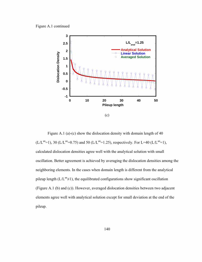
140

Figure A.1 continued

-1

-0.5

0

0.5

1

1.5

2

2.5

3

0 10 20 30 40 50

Analytical SolutionLinear SolutionAveraged Solution

Dis

loc

atio

n D

ensi

ty

Pileup length

L/Lanal

=1.25

(c)

Figure A.1 (a)-(c) show the dislocation density with domain length of 40

(L/Lan=1), 30 (L/Lan=0.75) and 50 (L/Lan=1.25), respectively. For L=40 (L/Lan=1),

calculated dislocation densities agree well with the analytical solution with small

oscillation. Better agreement is achieved by averaging the dislocation densities among the

neighboring elements. In the cases when domain length is different from the analytical

pileup length (L/Lan≠1), the equilibrated configurations show significant oscillation

(Figure A.1 (b) and (c)). However, averaged dislocation densities between two adjacent

elements agree well with analytical solution except for small deviation at the end of the

pileup.

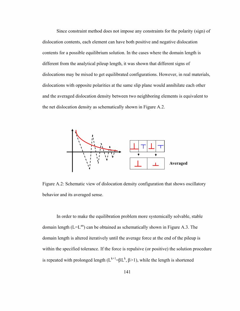
141

Since constraint method does not impose any constraints for the polarity (sign) of

dislocation contents, each element can have both positive and negative dislocation

contents for a possible equilibrium solution. In the cases where the domain length is

different from the analytical pileup length, it was shown that different signs of

dislocations may be mixed to get equilibrated configurations. However, in real materials,

dislocations with opposite polarities at the same slip plane would annihilate each other

and the averaged dislocation density between two neighboring elements is equivalent to

the net dislocation density as schematically shown in Figure A.2.

Averaged

Figure A.2: Schematic view of dislocation density configuration that shows oscillatory

behavior and its averaged sense.

In order to make the equilibration problem more systemically solvable, stable

domain length (L=Lan) can be obtained as schematically shown in Figure A.3. The

domain length is altered iteratively until the average force at the end of the pileup is

within the specified tolerance. If the force is repulsive (or positive) the solution procedure

is repeated with prolonged length (Lk+1=Lk, >1), while the length is shortened

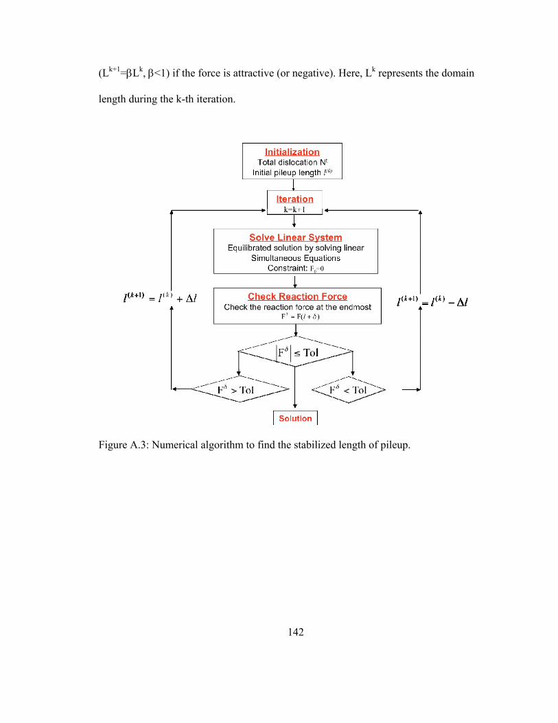
142

(Lk+1=Lk, <1) if the force is attractive (or negative). Here, Lk represents the domain

length during the k-th iteration.

Figure A.3: Numerical algorithm to find the stabilized length of pileup.

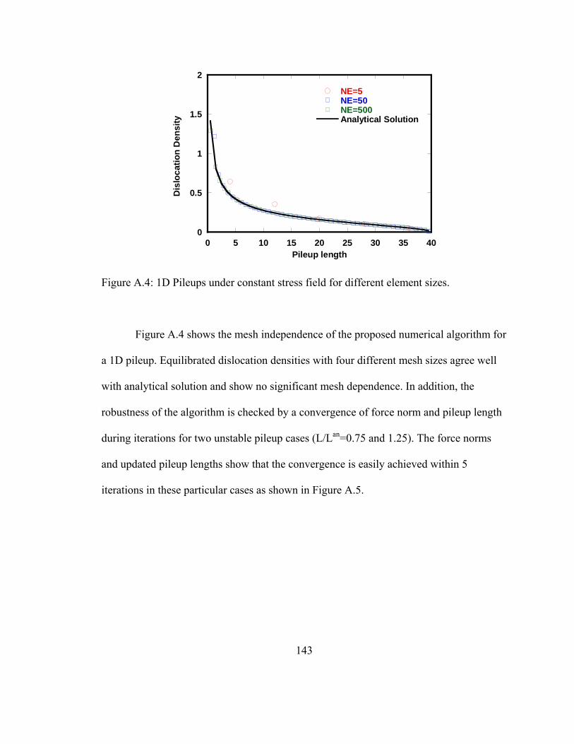
143

0

0.5

1

1.5

2

0 5 10 15 20 25 30 35 40

NE=5NE=50NE=500Analytical Solution

Dis

loc

atio

n D

ensi

ty

Pileup length

Figure A.4: 1D Pileups under constant stress field for different element sizes.

Figure A.4 shows the mesh independence of the proposed numerical algorithm for

a 1D pileup. Equilibrated dislocation densities with four different mesh sizes agree well

with analytical solution and show no significant mesh dependence. In addition, the

robustness of the algorithm is checked by a convergence of force norm and pileup length

during iterations for two unstable pileup cases (L/Lan=0.75 and 1.25). The force norms

and updated pileup lengths show that the convergence is easily achieved within 5

iterations in these particular cases as shown in Figure A.5.

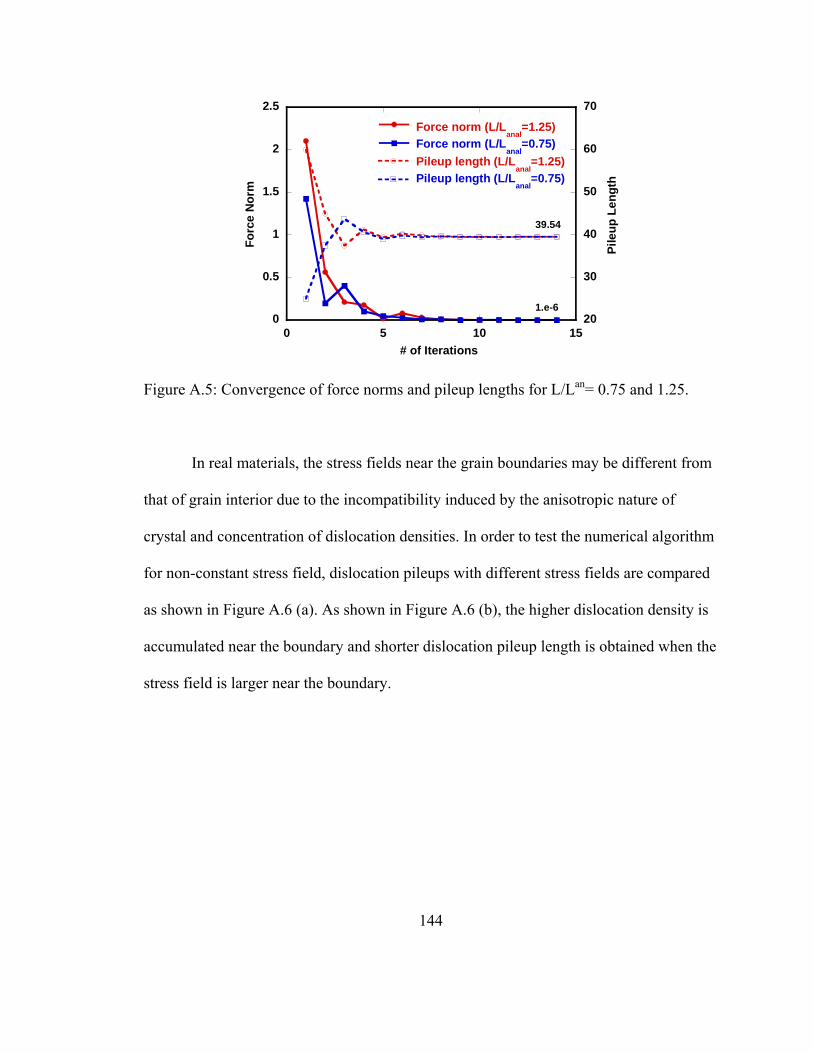
144

0

0.5

1

1.5

2

2.5

20

30

40

50

60

70

0 5 10 15

B

F

C

G

Fo

rce

No

rm

# of Iterations

Force norm (L/Lanal

=1.25)

Force norm (L/Lanal

=0.75)

Pileup length (L/Lanal

=1.25)

Pileup length (L/Lanal

=0.75)

Pile

up

Le

ng

th

39.54

1.e-6

Figure A.5: Convergence of force norms and pileup lengths for L/Lan= 0.75 and 1.25.

In real materials, the stress fields near the grain boundaries may be different from

that of grain interior due to the incompatibility induced by the anisotropic nature of

crystal and concentration of dislocation densities. In order to test the numerical algorithm

for non-constant stress field, dislocation pileups with different stress fields are compared

as shown in Figure A.6 (a). As shown in Figure A.6 (b), the higher dislocation density is

accumulated near the boundary and shorter dislocation pileup length is obtained when the

stress field is larger near the boundary.

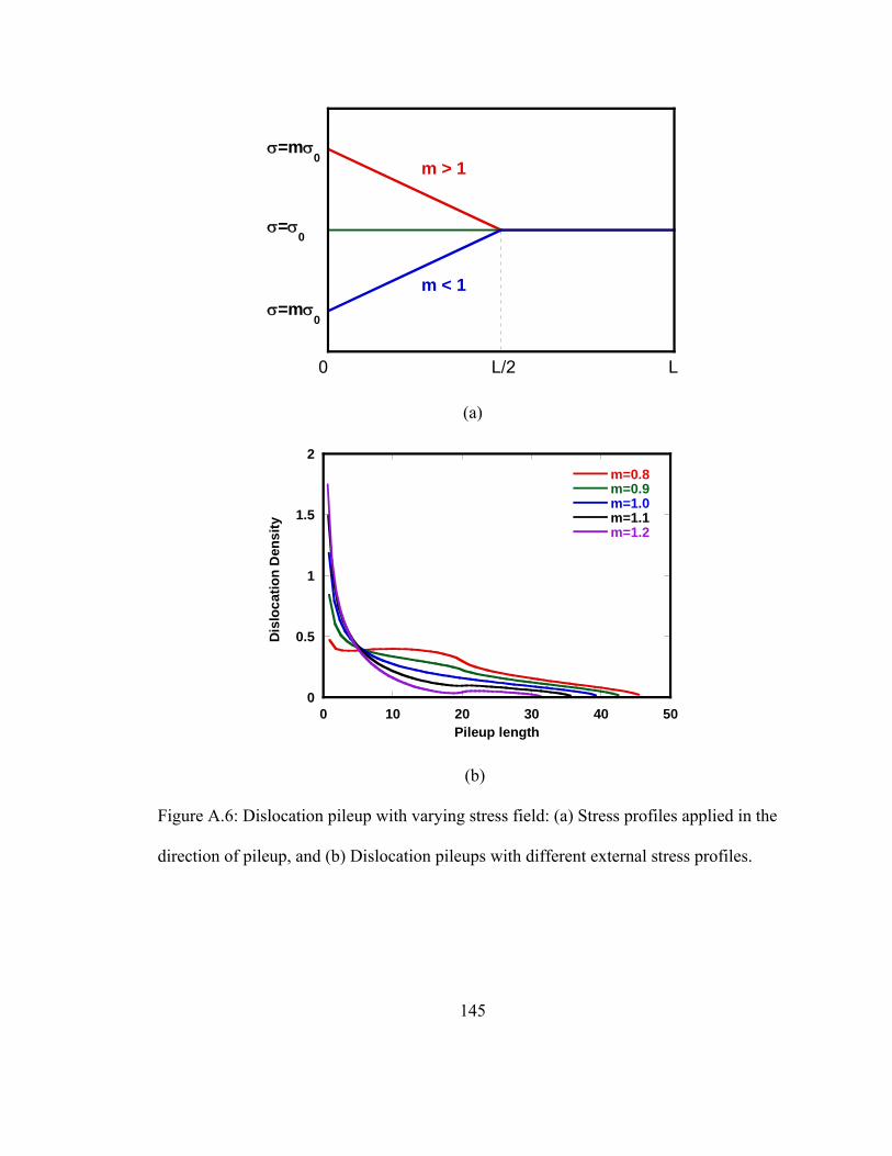
145

m > 1

m < 1

=m0

=0

=m0

L/2 L0

(a)

0

0.5

1

1.5

2

0 10 20 30 40 50

m=0.8m=0.9m=1.0m=1.1m=1.2

Dis

loc

atio

n D

ens

ity

Pileup length

(b)

Figure A.6: Dislocation pileup with varying stress field: (a) Stress profiles applied in the

direction of pileup, and (b) Dislocation pileups with different external stress profiles.

146

Alternative method to solve the equilibrium equation, equation (A.1) with the

superdislocation concept is to use energy minimization procedure as in Monte Carlo

method. The general equilibrium equation, equation (B.3), can be rewritten as:

12

1 1 10 ( 2, , )

2

EN

j i Eji i ji j

N N N i Nx x x

(A.3)

In order to obtain static solution, small fraction of dislocation content is moved

into neighboring element from the initial dislocation distribution and the norm of force

imbalance is checked. If the force norm is decreased compared with that of previous time

step, new distribution is accepted. This iterative procedure continues until the force norm

is within the prescribed tolerance. The brief summary of this algorithm is illustrated in

Figure A.7.

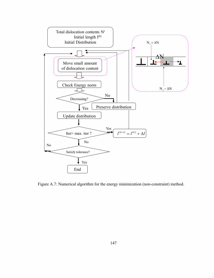
147

NNi

NN j

Total dislocation contents Nt

Initial length l(0)

Initial Distribution

Move small amount of dislocation content

Check Energy norm

Decreasing?No

Yes

Update distribution

Preserve distribution

No

Iter> max. iter ?

No

Satisfy tolerance?

Yes

Yes

End

lll kk )()1(

N

Figure A.7: Numerical algorithm for the energy minimization (non-constraint) method.

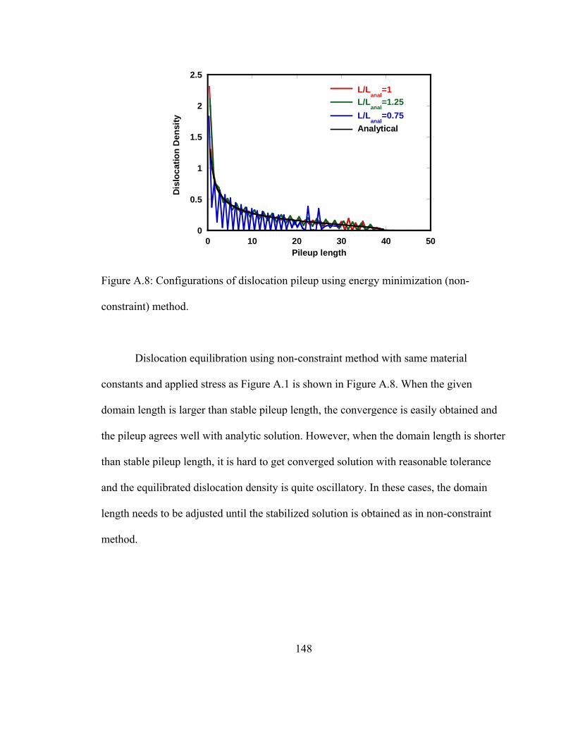
148

0

0.5

1

1.5

2

2.5

0 10 20 30 40 50

B

E

H

K

Dis

loc

atio

n D

ensi

ty

Pileup length

L/Lanal

=1

L/Lanal

=1.25

L/Lanal

=0.75

Analytical

Figure A.8: Configurations of dislocation pileup using energy minimization (non-

constraint) method.

Dislocation equilibration using non-constraint method with same material

constants and applied stress as Figure A.1 is shown in Figure A.8. When the given

domain length is larger than stable pileup length, the convergence is easily obtained and

the pileup agrees well with analytic solution. However, when the domain length is shorter

than stable pileup length, it is hard to get converged solution with reasonable tolerance

and the equilibrated dislocation density is quite oscillatory. In these cases, the domain

length needs to be adjusted until the stabilized solution is obtained as in non-constraint

method.

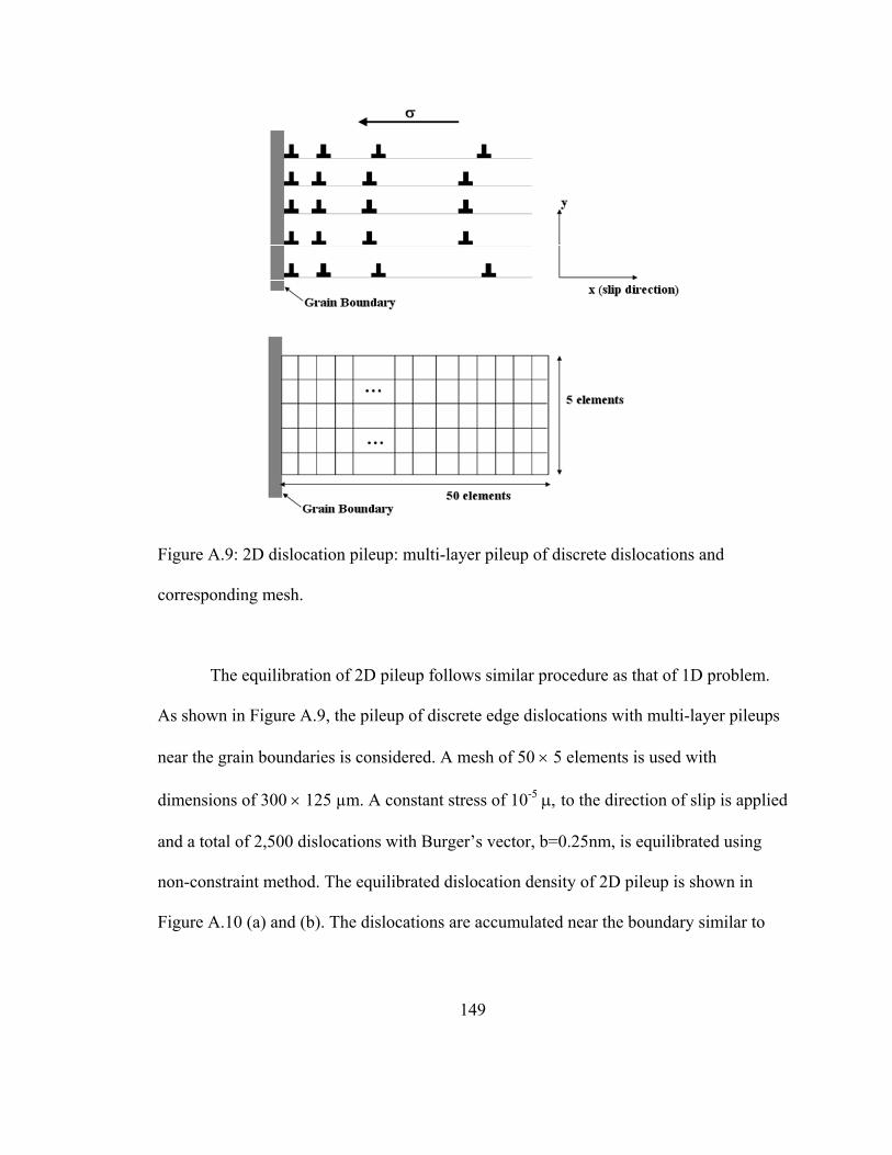
149

Figure A.9: 2D dislocation pileup: multi-layer pileup of discrete dislocations and

corresponding mesh.

The equilibration of 2D pileup follows similar procedure as that of 1D problem.

As shown in Figure A.9, the pileup of discrete edge dislocations with multi-layer pileups

near the grain boundaries is considered. A mesh of 50 5 elements is used with

dimensions of 300 125 µm. A constant stress of 10-5 to the direction of slip is applied

and a total of 2,500 dislocations with Burger’s vector, b=0.25nm, is equilibrated using

non-constraint method. The equilibrated dislocation density of 2D pileup is shown in

Figure A.10 (a) and (b). The dislocations are accumulated near the boundary similar to

150

1D pileup and the distribution along the y-direction is almost uniform in this particular

example as shown in Figure A.10 (b).

(a)

(b)

Figure A.10: 2D dislocation distribution in pileup under constant stress in the pileup

direction: (a) surface plot, and (b) profiles along constant y-path.

151

APPENDIX B: Interaction Force Between Two Edge Dislocation Segments

In this section, the glide force on an edge dislocation segment (1) by a parallel

edge dislocation segment (2) with parallel Burgers vectors is derived. The position vector

from the centers of segment (1) to segment (2) is zyx ˆˆˆ 321 rrrr

. 1dl and 2dl are

segment lengths; and the Cartesian coordinate system is as shown in Figure 4.3 ( x = glide

direction z = line direction). Following the approach of Hirth and Lothe (Hirth and Lothe,

1969), the force on dl1 by the segment y1y2 is given as

)()( 1112 xyxy FFF (B.1)

where F is a total force acting on dl1. When 12 yy ,

dy

xyd

yy

xyxy

dl

dyy

),(),(),(lim 1

12

1112

2 12

FFFF

(B.2)

By assuming Burgers vector is in 2e direction and considering only the glide component,

),( xyF can be represented as:

13

22

2

22

3

121

)(1

)()1(4),( dl

rRR

r

R

r

rRR

rbbxy

F

(B.3)

where 222

21 )( xyrrR . Equation (B.3) can be rewritten as:

N

k

kif

bbxyxy

1

211112 )1(4)(F)(FF

(B.4)

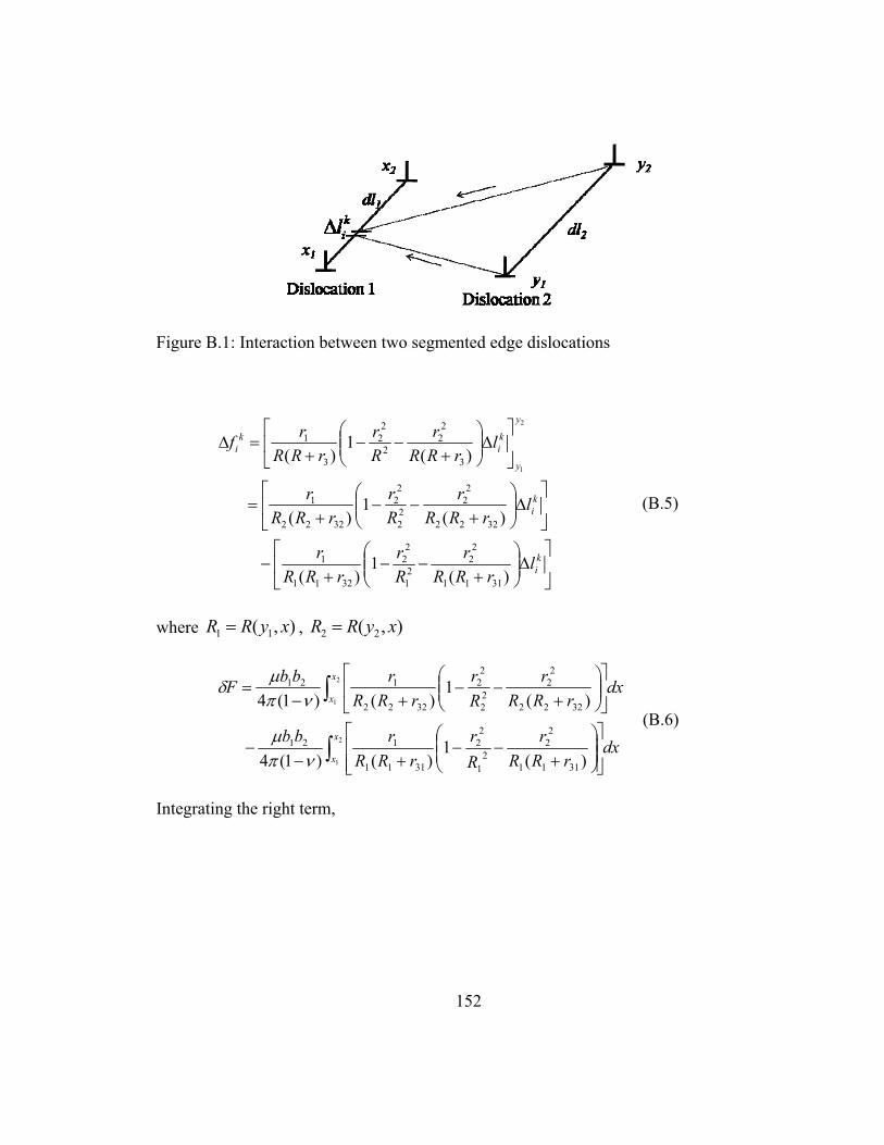
152

Figure B.1: Interaction between two segmented edge dislocations

ki

ki

y

y

ki

ki

lrRR

r

R

r

rRR

r

lrRR

r

R

r

rRR

r

lrRR

r

R

r

rRR

rf

)(1

)(

)(1

)(

)(1

)(

3111

22

21

22

3211

1

3222

22

22

22

3222

1

3

22

2

22

3

1

2

1

(B.5)

where ),( 11 xyRR , ),( 22 xyRR

dxrRR

r

R

r

rRR

rbb

dxrRR

r

R

r

rRR

rbbF

x

x

x

x

2

1

2

1

)(1

)()1(4

)(1

)()1(4

3111

22

21

22

3111

121

3222

22

22

22

3222

121

(B.6)

Integrating the right term,

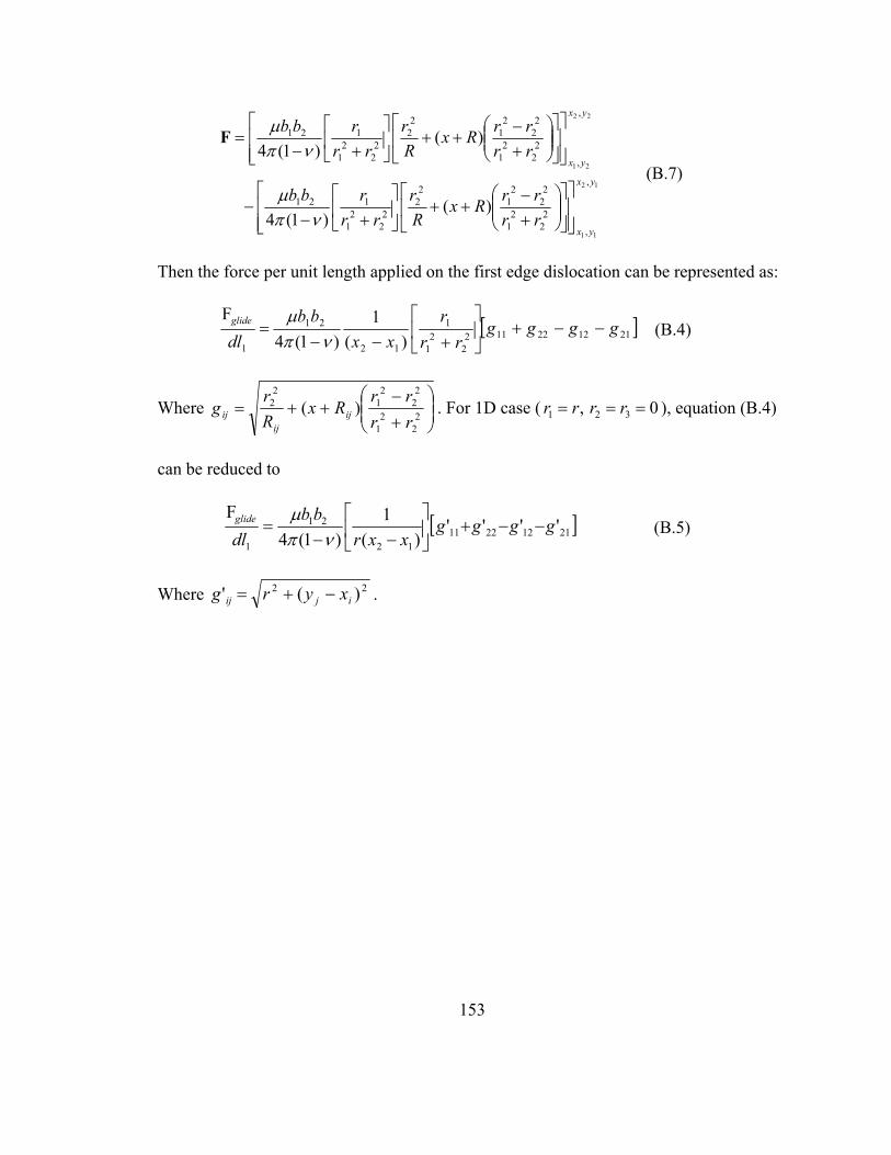
153

12

11

22

21

,

,

22

21

22

21

22

22

21

121

,

,

22

21

22

21

22

22

21

121

)()1(4

)()1(4

yx

yx

yx

yx

rr

rrRx

R

r

rr

rbb

rr

rrRx

R

r

rr

rbb

F

(B.7)

Then the force per unit length applied on the first edge dislocation can be represented as:

2112221122

21

1

12

21

1 )(

1

)1(4

Fgggg

rr

r

xx

bb

dlglide

(B.4)

Where

2

22

1

22

21

22 )(

rr

rrRx

R

rg ij

ijij . For 1D case ( 0, 321 rrrr ), equation (B.4)

can be reduced to

21122211

12

21

1

'''')(

1

)1(4

Fgggg

xxr

bb

dlglide

(B.5)

Where 22 )(' ijij xyrg .

154

APPENDIX C: Slip systems for FCC and BCC

FCC Slip system Slip normal Slip direction Slip system Slip normal Slip direction

1 (111) [110] 7 (111) [110]

2 (111) [101] 8 (111) [111] 3 (111) [01 1] 9 (111) [101] 4 (111) [110] 10 (111) [110] 5 (111) [101] 11 (111) [101]

6 (111) [01 1] 12 (111) [011]

BCC

Slip system Slip normal Slip direction Slip system Slip normal Slip direction

1 (011) [111] 13 (211) [111]

2 (101) [111] 14 (121) [111]

3 (110) [111] 15 (112) [111]

4 (011) [111] 16 (211) [111]

5 (101) [111] 17 (121) [111]

6 (110) [111] 18 (112) [111]

7 (011) [111] 19 (211) [111]

8 (101) [111] 20 (121) [111]

9 (110) [111] 21 (112) [111]

10 (011) [111] 22 (211) [111]

11 (101) [111] 23 (121) [111]

12 (110) [111] 24 (112) [111]

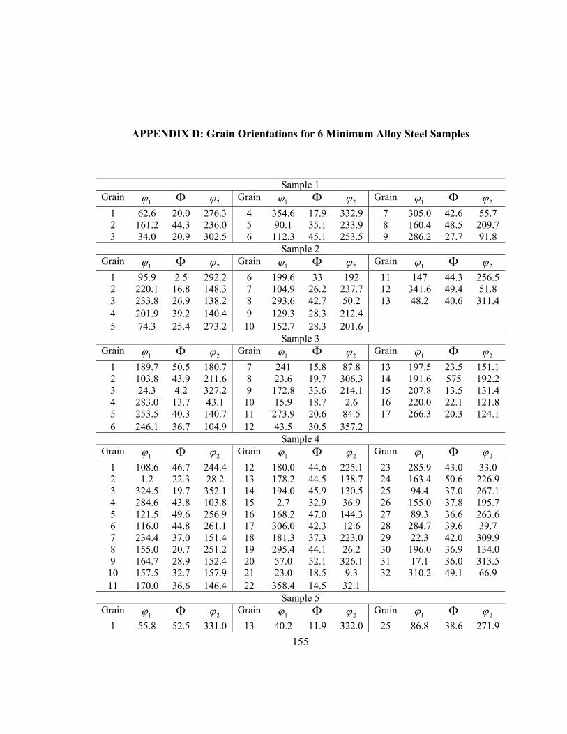
155

APPENDIX D: Grain Orientations for 6 Minimum Alloy Steel Samples

Sample 1Grain

1 2 Grain1 2 Grain

1 2

1 62.6 20.0 276.3 4 354.6 17.9 332.9 7 305.0 42.6 55.72 161.2 44.3 236.0 5 90.1 35.1 233.9 8 160.4 48.5 209.73 34.0 20.9 302.5 6 112.3 45.1 253.5 9 286.2 27.7 91.8

Sample 2Grain

1 2 Grain

1 2 Grain1 2

1 95.9 2.5 292.2 6 199.6 33 192 11 147 44.3 256.52 220.1 16.8 148.3 7 104.9 26.2 237.7 12 341.6 49.4 51.83 233.8 26.9 138.2 8 293.6 42.7 50.2 13 48.2 40.6 311.44 201.9 39.2 140.4 9 129.3 28.3 212.4 5 74.3 25.4 273.2 10 152.7 28.3 201.6

Sample 3Grain

1 2 Grain

1 2 Grain1 2

1 189.7 50.5 180.7 7 241 15.8 87.8 13 197.5 23.5 151.12 103.8 43.9 211.6 8 23.6 19.7 306.3 14 191.6 575 192.23 24.3 4.2 327.2 9 172.8 33.6 214.1 15 207.8 13.5 131.44 283.0 13.7 43.1 10 15.9 18.7 2.6 16 220.0 22.1 121.85 253.5 40.3 140.7 11 273.9 20.6 84.5 17 266.3 20.3 124.16 246.1 36.7 104.9 12 43.5 30.5 357.2

Sample 4Grain

1 2 Grain

1 2 Grain1 2

1 108.6 46.7 244.4 12 180.0 44.6 225.1 23 285.9 43.0 33.02 1.2 22.3 28.2 13 178.2 44.5 138.7 24 163.4 50.6 226.93 324.5 19.7 352.1 14 194.0 45.9 130.5 25 94.4 37.0 267.14 284.6 43.8 103.8 15 2.7 32.9 36.9 26 155.0 37.8 195.75 121.5 49.6 256.9 16 168.2 47.0 144.3 27 89.3 36.6 263.66 116.0 44.8 261.1 17 306.0 42.3 12.6 28 284.7 39.6 39.77 234.4 37.0 151.4 18 181.3 37.3 223.0 29 22.3 42.0 309.98 155.0 20.7 251.2 19 295.4 44.1 26.2 30 196.0 36.9 134.09 164.7 28.9 152.4 20 57.0 52.1 326.1 31 17.1 36.0 313.5

10 157.5 32.7 157.9 21 23.0 18.5 9.3 32 310.2 49.1 66.911 170.0 36.6 146.4 22 358.4 14.5 32.1

Sample 5Grain

1 2 Grain

1 2 Grain1 2

1 55.8 52.5 331.0 13 40.2 11.9 322.0 25 86.8 38.6 271.9

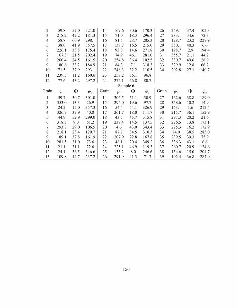
156

2 59.8 57.0 321.0 14 169.6 30.6 170.3 26 259.1 37.4 102.33 218.2 42.2 181.3 15 71.0 18.3 296.4 27 283.1 34.6 72.34 58.8 60.9 298.1 16 81.5 28.7 285.3 28 128.7 23.2 227.95 38.0 41.9 357.5 17 138.7 16.5 215.0 29 350.1 40.3 6.66 226.1 33.8 175.4 18 93.8 14.6 271.8 30 198.7 2.9 194.47 167.3 21.5 202.4 19 74.9 46.1 281.0 31 355.7 21.1 44.28 200.4 24.5 161.5 20 254.8 36.4 102.5 32 330.7 49.6 28.99 180.6 33.2 184.9 21 84.3 7.1 318.3 33 329.9 12.8 66.2

10 71.5 37.9 293.1 22 248.3 32.2 110.5 34 202.8 27.1 140.711 239.5 11.2 160.6 23 258.2 36.1 96.8 12 77.6 43.2 297.2 24 272.1 26.8 80.7

Sample 6Grain

1 2 Grain

1 2 Grain1 2

1 59.7 30.7 301.0 14 306.5 51.1 30.9 27 162.6 38.8 189.02 353.0 13.3 26.9 15 294.0 19.6 97.7 28 358.6 10.2 14.93 24.2 15.0 357.3 16 54.4 54.1 326.9 29 163.1 1.6 212.44 326.9 37.9 40.8 17 261.7 18.0 111.7 30 215.7 36.1 152.95 44.9 52.9 299.0 18 43.5 45.7 315.8 31 297.3 20.2 21.66 318.7 9.0 61.2 19 237.4 14.5 137.5 32 226.5 13.8 173.17 293.8 29.0 106.5 20 4.6 43.0 343.4 33 225.3 16.2 172.98 218.1 23.4 129.7 21 87.7 34.5 310.3 34 74.0 38.5 285.09 189.1 37.8 161.9 22 207.9 22.8 167.8 35 239.5 39.3 75.9

10 281.5 31.0 73.6 23 48.1 20.4 349.2 36 336.3 43.1 6.611 21.1 31.1 22.6 24 225.1 46.9 119.3 37 260.7 20.9 124.612 24.1 36.5 346.6 25 133.2 8.0 246.6 38 134.6 15.0 204.713 109.8 44.7 237.2 26 291.9 41.3 71.7 39 102.4 36.8 287.9