homogenization of the hamilton-jacobi …sorrenti/homepage_files/homogenizationhj.pdf ·...
TRANSCRIPT

HOMOGENIZATION OF THE HAMILTON-JACOBI EQUATION
ALFONSO SORRENTINO
Abstract. Since the celebrated work by Lions, Papanicolaou and Varadhan in 1980’s, therehas been a considerable attention to the homogenization problem for Hamilton-Jacobi equation:
roughly speaking, how to describe what macroscopic properties and aspects of this equationsurvive, once all of its local features are neglected (for example, by averaging over faster and
faster oscillations). The interest in this question – besides the importance of the Hamilton-Jacobi
equation in many different contexts (classical mechanics, symplectic geometry, PDEs, etc...) –has been in recent years boosted by the manifold connections that it shares with new prominent
areas of research: Aubry-Mather theory, weak KAM theory, symplectic homogenization, just to
mention a few of them.In this article, we discuss a very natural and important question, namely how to extend these
classical results beyond the Euclidean setting, which has been recently addressed in a work by
Contreras, Iturriaga and Siconolfi. Starting from their result and from the above-mentioned workby Lion, Papanicolaou and Varadhan, we first describe how both of them can be interpreted as a
particular case of a more intrinsic and geometric approach, i.e., the case of Tonelli Hamiltonians
which are invariant under the action of a discrete group. In particular, we point out the leadingrole played by the algebraic nature of the group (more specifically, its rate of growth) in driving
the homogenization process and determining the features of the limit problem. Then, we prove ahomogenization result in the case of Hamiltonians that are invariant under the action of a discrete
(virtually) nilpotent group (i.e., with polynomial growth).
Besides being more intrinsic and geometric, this novel approach provides a much clearer un-derstanding of the structures of both the limit space and the homogenized equation, unveiling
features and phenomena that in the previously-studied cases were shadowed by either the homo-
geneity of the ambient space or the abelianity of the acting group.
1. Introduction
Since the celebrated work by Lions, Papanicolaou and Varadhan [30], there has been a con-siderable attention to the homogenization of Hamilton-Jacobi equation and, more generally, tohomogenization problems. This increasing interest is justified by the wide spectrum of applica-tions, particularly to all of those models characterized by the coexistence of phenomena of differentscales and diverse complexities. Naively speaking, one aims at describing the macroscopic behaviourand the global picture of these problems, by averaging over their microscopic oscillations and ne-glecting their local features: in a pictorial sense, the goal is to single out what remains visible toa (mathematical) observer, as her/his point of view moves farther and farther away. One of theadvantage of this large scale description is that it is expected to be easier to study and possiblyto implement (for example, numerically); at the same time, this model continues to encode much
Date: November 11, 2015.2010 Mathematics Subject Classification. 35B27, 35B40, 35F21, 74Q10 (primary), and 20F69, 22E25, 35R03,
37J50 (secondary).
1

2 ALFONSO SORRENTINO
interesting information on the original (non-homogenized) problem.
1.1.1. The Hamilton-Jacobi Equation. Let us start by briefly recalling what is the classical Hamilton-Jacobi Equation1. It consists of a first-order nonlinear partial differential equation of the form
∂tu(x, t) +H(x, ∂xu(x, t)) = 0
where H : Rn×Rn −→ R is called the Hamiltonian and (x, t) ∈ Rn×R are independent variables.2
This equation can be easily defined on a general manifold M :
∂tu(x, t) +H(x, ∂xu(x, t)) = 0
where H : T ∗M −→ R is now defined on the cotangent bundle of M and (x, t) ∈ M × R continueto be independent variables.
This equation has many applications in dynamical systems and classical mechanics; its solutions,for example, are related to the existence of Lagrangian submanifolds that are invariant under theassociated Hamiltonian flow (e.g., KAM tori) and could be used, at least in principle, as generatorsof canonical (i.e., symplectic) changes of coordinates that simplify the equations of motion andmake them explicitly integrable. These special solutions – which are known to exist only underspecial circumstances – are the subject of the so-called KAM theory (named after the Kolmogorov,Arnol’d, and Moser).
Besides Hamiltonian dynamics, the Hamilton-Jacobi equation arises in many other differentcontexts, including: PDEs, calculus of variations, control theory, optimal mass transportationproblems, conservation laws, classical limits of Schrodinger equation, semi-classical quantum theory,etc... See for example [1, 5, 16, 29, 20, 5].
1.1.2. Classical Homogenization: the Euclidean Periodic Setting. Let us start by recalling a simplemodel of homogenization introduced and discussed by Lions, Papanicolaou and Varadhan in [30].Let H : Rn × Rn −→ R be a C2 Hamiltonian that is Zn-periodic in the space variables x, strictly
convex in the fiber-variables/momenta p (in the C2 sense, i.e., ∂2
∂p2H(x, p) is positive definite ev-
erywhere) and superlinear in each fiber.3 Observe that such a Hamiltonian can be seen as the liftof a Hamiltonian defined on Tn × Rn ' T ∗Tn; using a more modern terminology, we would call ita Tonelli Hamiltonian (see subsection 2.2).
The homogenization problem is related to understanding the limit behaviour of solutions tothe Hamilton-Jacobi equation, when the Hamiltonian is modified in order to have faster and fasteroscillatory spatial dependence. More specifically, for small ε > 0 one considers the rescaled equation
(1)
∂tu
ε(x, t) +H(xε , ∂xuε(x)) = 0 x ∈ Rn, t > 0
uε(x, 0) = fε(x).
1Sir William Rowan Hamilton (1805-1865) introduced this equation in his studies of geometrical optics in an arbi-trary medium with varying index of refraction. Later, Carl Gustav Jacob Jacobi (1804-1851) sharpened Hamilton’s
formulation and clarified some mathematical issues, making significant applications to classical mechanics.2Actually, more general versions could be considered; for instance, one could include parameters or choose the
right-hand side to be a non-vanishing function. For example:
∂tu(x, α, t) +H(x, α, ∂xu(x, α, t)) = K(α, t),
where (x, α, t) ∈ Rn × Rn × R are independent variables and K : Rn × R −→ R plays the role of an integrable
Hamiltonian.3Actually, the result in [30] is stated under less stringent hypothesis on the Hamiltonian. We restrict ourselves
to this setting, because we are interested in applying methods coming from Aubry–Mather theory and Lagrangian
dynamics.

HOMOGENIZATION OF THE HAMILTON-JACOBI EQUATION 3
It is a well-known result [27, 11] that if fε ∈ C(Rn) and has linear growth, then there exists aunique viscosity solution4 to the above problem. In [30] the authors studied what happens to thesesolutions as ε goes to 0, under the (natural) condition that in the limit fε converge uniformly to acontinuous function f with linear growth. In particular, they proved that the solutions uε convergelocally uniformly to the unique viscosity solution u of the limit (or homogenized) problem:
(2)
∂tu(x, t) +H(∂xu(x)) = 0 x ∈ Rn, t > 0u(x, 0) = f(x),
where H : Rn −→ R is a convex Hamiltonian (not necessarily strictly convex) which does notdepend on x; H is called effective (or homogenized) Hamiltonian. While H is usually highly non-differentiable, nevertheless the solution u of the limit problem are very easy to describe, since thecharacteristic curves for the limit equation are straight lines: for each x ∈ Rn and t > 0
(3) u(x, t) = miny∈Rn
f(y) + tL
(x− yt
),
where L : Rn −→ R is the Legendre-Fenchel transform of H (or effective Lagrangian), given byL(v) := maxp∈Rn
p · v −H(p)
.
Let us point out what are the main steps that characterize the homogenization process (thisaspect will be of crucial importance in order to extend these results to a more general setting):
H1. Determine the space and the setting to consider; in [30] the authors considered Rn withZn-periodic conditions (i.e., lifts of Tonelli Hamiltonian on T ∗Tn to the universal coverRn × Rn).
H2. Rescale the equation in order to increase the oscillations of the space variables; in theprevious discussion, this was achieved by multiplying the space variables by a parameterε→ 0+ (see (1)).
H3. Determine the limit problem, e.g. the homogenized Hamiltonian H and the space on whichit is defined; in the previous case, H was also defined on Rn. See subsection 1.1.3 for amore detailed discussion on H.
H4. Describe the solutions to the limit problem (see (3)).H5. Prove the convergence of the solutions to the rescaled problem to the solution to the limit
one (i.e., uε −→ u locally uniformly as ε→ 0+).
1.1.3. The Homogenized Hamiltonian. The identification of the effective Hamiltonian is definitelyan important step in the homogenization procedure. In [30], H : Rn −→ R was obtained bystudying the so-called cell problem (or stationary ergodic Hamilton-Jacobi equation, see equation(4)), an auxiliary equation arising in the formal expansion in ε of (2). More specifically, for eachp ∈ Rn, there exists a unique λ ∈ R for which the following equation admits a viscosity (periodic)solution v : Rn −→ R:
(4) H(x, p+ ∂xv(x)) = λ x ∈ Rn.
We denote such a value λ by H(p), thus defining H : Rn −→ R; see [30, Theorem 1]. Observethat this equation can be thought as a nonlinear eigenvalue problem with the effective Hamiltonian
4The concept of viscosity solution concept was introduced in the early 1980’s by Pierre-Louis Lions and Michael
G. Crandall as a generalization of the classical concept of solution to a partial differential equation and is based onthe maximum principle for PDE’s. We refer interested readers, for example, to [10, 21].

4 ALFONSO SORRENTINO
H(p) and the solution v playing respectively the roles of the eigenvalue and the eigenfunction.
This description of the effective Hamiltonian can be generalized to the case of a Hamiltoniandefined on the cotangent bundle of an arbitrary compact manifold M (see for example [12, 24]);the previous example – because of the periodicity assumption – corresponds to the case M = Tnand T ∗M = Tn × Rn. However, a general compact manifold M is not necessarily parallelizable,therefore one should pay attention to how replace the role of p (i.e., the argument of the effectiveHamiltonian) in (4).
Let us start by remarking that looking for a (smooth) periodic solution v of (4) is equivalent tosearching a closed 1-form on Tn with cohomology class p, whose graph is contained in an energylevel of the Hamiltonian H (the graph of a 1-form corresponds in fact to a section of T ∗Tn). Hence,the change of p can be interpreted as searching for solutions with different cohomology classes (re-call that H1(Tn;R) ' Rn).
Let now M be a general smooth compact manifold without boundary and let H : T ∗M −→ Rbe a Tonelli Hamilonian, i.e., a C2 Hamiltonian, which is strictly convex and superlinear in eachfiber (see subsection 2.2 for a more precise definition). Then one can define the associated effectiveHamiltonian in the following way:
- Let η be a closed 1-form on M and let [η] ∈ H1(M ;R) denote its cohomology class.- There exists a unique λ ∈ R for which the following equation admits a viscosity solution v
(see [12, 24]):
(5) H(x, η(x) + dxv(x)) = λ x ∈M.
- Clearly, this unique value λ does not depend on η, but only on its cohomology class. Infact, if η and η′ are two closed 1-forms with [η] = [η′], then η − η′ is exact and thereforethere exists w : M −→ R such that η − η′ = dw, which will affect only the form of thesolution and not the energy value.
- We denote this unique value of λ by H([η]), hence defining a function
H : H1(M ;R) −→ Rthat will be called effective Hamiltonian.
Remark 1.1. It is important to recall that H1(M ;R) ' Rb1(M), where b1(M) denotes the firstBetti number of M . In general, differently from what happens in the euclidean periodic case, thereis no relation between the dimension of M and b1(M), so the effective Hamiltonian is defined ona space that can have a drastically larger or smaller dimension. For example, if M is a surface ofgenus g ≥ 0, then b1(M) = 2g, which can be arbitrary larger than dimM = 2.
1.1.4. Digression: The Effective Hamiltonian and Mather–Mane Theory. It turns out that theeffective Hamiltonian – that we have defined in subsection 1.1.3 in terms of the solutions to the cellproblem – is also extremely significant from a dynamical systems point of view, particularly in thestudy of the associated Hamiltonian dynamics by means of variational methods: what is nowadaysknown as Mather and Mane theory. We refer interested readers to [33, 32, 13, 41] for more detailedpresentations of these topics.
Roughly speaking, this theory is based on the study of particular orbits and invariant measures ofthe flow that are obtained as minimizing solutions to variational problems related to the so-calledPrinciple of least (Lagrangian) action. As a result of this, these objects present a much richer

HOMOGENIZATION OF THE HAMILTON-JACOBI EQUATION 5
structure and rigidity than one might generally expect, and the corresponding invariant sets – theso-called Mather, Aubry and Mane sets – play an important role in determining both the local andthe global dynamics of the system.
In this setting, the value of the effective Hamiltonian appears in many noteworthy forms and hasconsequently been named in different ways by the various communities: minimal average action,Mather’s α-function, Mane critical values, etc...
Let us briefly recall some of these definitions. In what follows, let L : TM −→ R denote theLagrangian associated to H (given by Legendre-Fenchel duality) and for any cohomology classc ∈ H1(M ;R) let us consider a closed 1-form ηc representing it (it is easy to check that the defini-tions below do not depend on the chosen representative, but only on their cohomology class). Then:
1) If ML denotes the set of invariant probability measures for the Euler-Lagrange flow associ-ated to L, then:
H(c) = − minµ∈ML
∫TM
(L(x, v)− ηc(x) · v) dµ.
The value of the right-hand side is usually denoted by α(c) and the collection of these valuesα : H1(M ;R) −→ R is what is known as Mather’s α-function or Mather’s minimal averageaction.
2) For any absolutely continuous curve γ : [a, b] −→M , we define its L-action as
AL,ηc(γ) :=
∫ b
a
(L(γ(t), γ(t))− ηc(γ(t)) · γ(t)
)dt.
Then:
H(c) = infk ∈ R : AL+k,ηc(γ) ≥ 0, ∀ abs. cont. loop γ= supk ∈ R : AL+k,ηc(γ) < 0 for some abs. cont. loop γ .
The values on the right-hand sides are often called Mane critical values.
3) In [8] Dias Carneiro proved that H(c) represents the energy (i.e., the value of the Hamil-tonian) of action-minimizing measures or action-minimizing orbits of cohomology class c.
4) It was proved in [38] that H(c) represents the infimum of the energy values k’s such thatthe energy sublevel H(x, p) ≤ k contains in its interior a smooth Lagrangian graph ofcohomology class c. In particular, it corresponds to the smallest energy sublevel containingLipschitz Lagrangian graphs of cohomology class c.
Remark 1.2. Finally, it is also interesting to observe that the homogenized Hamiltonian H coin-cides with the symplectic homogenized Hamiltonian defined by Viterbo in [44] for Hamiltonians onT ∗Tn. This definition was later extended to Hamiltonian on general compact manifolds in [36].
1.1.5. How to Homogenize on a General Manifold. We want now to address the main (and verynatural) question at the core of this work: how to generalize Lions, Papanicolaou and Varadhan’s

6 ALFONSO SORRENTINO
result to the case of (Tonelli) Hamiltonians defined on more general spaces, not necessarily euclidean.
In the light of the homogenization steps H1-5 singled out in subsection 1.1.2, we need to addressthe following questions:
Q1 - How to rescale a general Hamilton-Jacobi equation?Q2 - How to define the homogenized Hamiltonian H? In particular, on which space should the
limit problem be defined?Q3 - How to intend (and prove) the convergence of solutions to the limit one?
Q1. Let us start by discussing the first question, which is relatively easy to address. As suggestedin [14], let us observe that in the euclidean periodic case (i.e., on Tn) if uε is a solution to therescaled Hamilton-Jacobi equation (1), then vε(x, t) := uε(εx, t) is a Zn-periodic solution to
(6) ∂tvε(x, t) +H
(x,
1
ε∂xv
ε(x, t)
)= 0 x ∈ Rn, t > 0.
This equation – which is indeed equivalent to (1) – can be interpreted in the following geometricway: we do not rescale the space variables, but we consider a rescaled metric on it (which affectsonly the momenta). Observe that equation (6) corresponds to Hamilton-Jacobi equation on themetric space (Tn, dε := εdeucl), where deucl denotes the euclidean metric on Tn. The advantage ofthis formulation of the problem is that this makes sense on a general metric space, whereas rescalingthe space variables is possible only on spaces equipped with dilations, or having a homogeneousstructure.
Hence, if X is a smooth connected (not necessarily compact) manifold without boundary, en-dowed with a complete Riemannian metric d and H : T ∗X −→ R is a Hamiltonian, then for eachε > 0 we shall consider the following rescaled Hamilton-Jacobi equation:
∂tvε(x, t) +H(x, 1
ε∂xvε(x, t)) = 0 x ∈ X, t > 0
vε(x, 0) = fε(x),
where fε : X −→ R is a function on the rescaled metric space Xε := (X, dε := εd) (of course, morehypothesis will be needed in order to prove a homogenization result).
Q2 & Q3. The second and third questions are definitely less straightforward and – as we shall seelater – they will represent the core of this article (in particular, see section 3 for Q3 and section 4for Q2).
Actually, a more fundamental (and urgent) question should be:
Q0 - What setting to consider?
To the best of our knowledge, the only article in which this latter issue has been addressed beforeis [14], where the authors consider a closed manifold M and discuss how to extend classical homog-
enization results for litfs of Tonelli Hamiltonians on the cotangent bundle of its abelian cover M(observe that Rn corresponds to both the universal and the abelian cover of Tn). In what follows,

HOMOGENIZATION OF THE HAMILTON-JACOBI EQUATION 7
we shall start by recalling the reasons justifying this choice and we shall later propose a different,more general, setting that we believe better suits the nature of the problem.
1.1.6. Homogenization on the Abelian Cover. Let us summarize the main result and ideas in [14]. Aswe have discussed in subsections 1.1.3 and 1.1.4, for Tonelli Hamiltonian T ∗M , where M is a closedmanifold, there is a natural candidate for the homogenized Hamiltonian, H : H1(M ;R) −→ R.However, there is a crucial obstacle that one has to consider: while this limit Hamiltonian H isdefined on H1(M ;R), the rescaled solutions are functions on M ; the problem of convergence ismade even more critical by the fact that – as we have pointed out in Remark 1.1 – these spaceshave different dimensions (this difference might be very large!).
Inspired by a strategy that had already been exploited in the context of Mather’s theory (seefor example [15, 22, 33, 34]), the authors propose to solve this problem by considering the liftof the Hamiltonian to the so-called (maximal free) abelian cover of M , i.e., the covering space
of M whose fundamental group is π1(M) = ker h, where h denotes the Hurewicz homomorphismπ1(M) −→ H1(M ;R), and whose group of deck transformations is isomorphic to the free part ofH1(M ;Z), i.e., Zb1(M) with b1(M) := dimH1(M ;R).
Observe that the lifted Hamiltonian H : T ∗M −→ R satisfies a sort of “periodicity” property:it is invariant under the action of the group of deck transformations. Hence, one can identify some“privileged” directions, which are not canceled by the rescaling process. Figuratively speaking,as one looks as the manifold from far away (i.e., rescales the metric by a parameter that goes tozero), while all local properties pass out of sight, these “homological directions” remain clearly
identifiable. Then, in some sense, M has a (homological) “structure” like Zb1(M) and consequentlythe ε-rescaled metric space has a structure like εZb1(M), which, as ε goes to zero, becomes moreand more similar to Rb1(M) ' H1(M ;R).
This idea allowed the authors of [14] to define a “homological” coordinate map G : M −→H1(M ;R) (which depends, of course, on a reference point in M and on the choice of a basis ofH1(M ;R), like a sort of “homological compass”) and to give a meaningful notion of convergence
of (M, εd) to H1(M ;R) (where d denotes the lifted metric), as well as a notion of convergence of
functions on M to functions defined on H1(M ;R); see [14, Section 2] for more details.
Theorem (Contreras, Iturriaga and Siconolfi, [14]). Let M be a closed manifold, H : T ∗M −→ Ra Tonelli Hamiltonian and let H : T ∗M −→ R denote the lift of H to the cotangent bundle of the
maximal free abelian cover M . Let fε : M −→ R and f : H1(M ;R) −→ R be continuous maps, with
f of at most linear growth, and assume that fε converge uniformly to f . Let vε : M× [0,+∞) −→ Rbe the viscosity solution to the problem
∂tvε(x, t) +H(x, 1
ε∂xvε(x, t)) = 0 x ∈ M, t > 0
vε(x, 0) = fε(x).
Then, the family of functions vε converges locally uniformly in M×(0,+∞) to the viscosity solutionv : H1(M ;R)× [0,+∞) −→ R of the homogenized problem:
∂tv(x, t) +H(∂xv(x, t)) = 0 x ∈ H1(M ;R), t > 0v(x, 0) = f(x),
where the effective Hamiltonian H : H1(M ;R) −→ R coincides with Mather’s α-function.

8 ALFONSO SORRENTINO
Moreover, there is a representation formula for v:
v(x, t) = miny∈H1(M ;R)
f(y) + tL
(x− yt
)for x ∈ H1(M ;R), t > 0,
where L : H1(M ;R) −→ R denotes the effective Lagrangian associated to H, i.e., its Legendre-Fenchel transform (also known as Mather’s β-function).
Remark 1.3. i) The notion of convergence in the above statement must be understood in thesense introduced in [14, Section 2], which is reminiscent of (pointed) Gromov–Hausdorff conver-gence for (non-compact) metric spaces (see section 3.1 and [7]). Very roughly speaking, using the
map G : M −→ H1(M ;R), one can transpose the problem to H1(M ;R) ' Rb1(M).ii) Observe that while the limit function v(·, t) is defined on H1(M ;R), the homogenized Hamilton-ian H is defined on H1(M ;R). In fact, the argument of H is the differential of u(·, t) which is anelement of the dual space (H1(M ;R))∗ ' H1(M ;R).iii) In [14] the authors also discuss the case in which the Hamiltonian is lifted to a non-maximalfree abelian cover and obtain similar results.
This theorem automatically raises a very natural question: is there any reason why one has toconsider the abelian cover of M and lift the problem to this space?
First of all, it is clear that the homogenization process must take place in a non-compact manifold,otherwise it would lead to a trivial result in the limit as the rescaling parameter goes to 0. Forinstance, in [30] the authors consider the problem not on Tn, as one could think, but on Rn withZn-periodicity conditions.
Yet, there are many other non-compact covers of M and many possible periodicity conditions:what makes the abelian cover special or preferable?
From a technical point of view, this choice has the advantage of transforming the problem into aproblem on the euclidean space Rb1(M) ' H1(M ;R) and makes possible to exploit the homogeneityof this space to provide a meaningful notion of convergence and extend classical results. Moreover,the ideas and techniques used in the proof, are crucially dependent on the abelianity of this group(i.e., of the group of the deck transformations of the abelian cover).
On the other hand, apparently this choice seems to be the natural one, if one wishes the ho-mogenized Hamiltonian H to be defined on H1(M ;R), as it is reasonable to expect in the light ofwhat discussed in subsection 1.1.3. However, one could ask her/himself whether the fact that H isdefined on H1(M ;R), necessarily requires the solution v to be defined on H1(M ;R).
1.1.7. Beyond the Abelian Case. In order to address the above issues and try to investigate towhich extent the homogenization process can be generalized to general manifolds (hence providinga satisfactory answer to Q0), it is useful to reinterpret the result in [14] (and therefore the classicalone in [30]) in a different way. In particular, this different point of view presents the advantage ofremoving – or, at least, hiding – the arbitrariness of the choice of the cover to which one lifts H;moreover, it is closer to the spirit of the classical result in [30] (where no lift to a covering space is

HOMOGENIZATION OF THE HAMILTON-JACOBI EQUATION 9
involved, since the periodicity condition is assigned a-priori).
Let us start by observing that the lifted Hamiltonian H : T ∗M −→ R is still a Tonelli Hamilton-ian (it is strictly convex and superlinear in each fiber) and has the property of being invariant under
the action of the group of deck transformations Γ := Aut(M,M) ' Zb1(M) (to be more precise, itis invariant under the lifted action of Γ to the cotangent bundle; see subsection 2.2). This actionenjoys many good properties (see subsection 2.1), which essentially come from the fact that the
quotient Γ\M is a closed manifold (in this specific case, this quotient coincides with M) and thatthe covering map is regular.
Hence, we believe that the most natural setting to generalize this homogenization result is thefollowing:
• Let X be a smooth connected (non-compact) manifold without boundary, endowed with a
complete Riemannian metric d; in the previous case, X = M .• Let Γ be a finitely generated (torsion free) group, which acts smoothly on X by isometries
(in other words, the metric d is the lift of a metric on the quotient space Γ\X); in the
previous case, Γ := Aut(M,M) ' Zb1(M).• Suppose that this action is free, properly discontinuous and co-compact (i.e., the quotient
space Γ\X is a compact manifold); in the previous case, these properties were clearlysatisfied.
• Let H : T ∗X −→ R be a Tonelli Hamiltonian. The lifted action of Γ to T ∗X is given by
Γ× T ∗X −→ T ∗X
(γ, (x, p)) 7−→ γ · (x, p) := (γ(x), p dγ(x)γ−1).
We require that H is invariant under this action, namely
H(x, p) = H(γ(x), p dγ(x)γ−1) ∀ (x, p) ∈ T ∗X and ∀ γ ∈ Γ.
Our aim in the following sections is to provide an answer to this question:
Is it possible to prove in this setting a homogenization result for the associated Hamilton-Jacobiequation?
We shall see that the answer to this question profoundly depends on the algebraic nature ofthe group Γ, more specifically, on its rate of growth (see subsection 3.2.1). Let us provide first avery sketchy idea on the role of Γ and on how it intervenes in this process (see subsection 3.2.1 formore details). Let us start with the following observation. When we look at a metric space (X, d)from “far away”’ (i.e., we rescale the metric by a small positive parameter ε and let it go to zero),although no local property survive, yet one can still try to describe the asymptotic shape and theasymptotic properties of this “limit” space, if any limit exists (see Definition 3.6). The key point isthat these asymptotic information will be the same for metric spaces that are “close” or “similar”enough; more precisely, for metric spaces that are at finite Gromov-Hausdorff distance from eachother (see section 3).

10 ALFONSO SORRENTINO
In our specific case, since Γ is acting on X and the action satisfies all of the above properties,then each orbit Γ · x0 can be seen as a copy of Γ embedded in X; in particular, as ε goes to zero,this copy becomes denser and denser in X with respect to the rescaled metric.
Hence, instead of looking at the behavior of (X, d), one can consider Γ equipped with somesuitable distance dΓ, and study how this new metric space behaves under rescaling; this limit space– when it exists – is called the asymptotic cone of Γ. The existence of this limit space and itsuniqueness are very subtle issues; as it turns out, a positive answer to these questions stronglydepends on the algebraic nature of the group, in particular on its rate of growth, which must be atmost polinomial (we shall describe these results and provide useful references in subsection 3.2.1).In the following we shall consider discrete free groups with polinomial growth, more specifically,torsion free nilpotent groups.
Remark 1.4. The fact that the growth of Γ must be at most polynomial should not be too supris-ing. For example, there is a very tight link between the rate of growth of the fundamental group ofa compact manifold M and the rate of growth of the volume of balls on its universal cover X (inthis case, π1(M) plays the role of Γ); see for example [18] and Remark 3.9. How the volume of ballson X grows is definitely a significant piece of information in order to study the homogenizationprocess and to show the the convergence of the rescaled solutions.
In light of this, it is very clear that the leading role in driving the homogenization process andin determining the structure of the limit space and of the homogenized equation, is played by the“periodicity” of the Hamiltonian (i.e., the acting group Γ), and not by the fundamental domainof this action (i.e., the compact quotient Γ\X). Somehow, this also better justifies the name “ho-mogenization”. In particular, lifting a Tonelli Hamiltonian from a compact manifold to its abeliancover, corresponds to choosing of a specific periodic extension of the Hamiltonian, yet not unique,nor necessarily more natural than others.
1.1.8. Main Results. Let us now describe our result on the homogenization of the Hamilton-Jacobiequation. The setting is the one that we have described in the previous subsection and, as we haveremarked above, it is important to impose a condition of the growth of the discrete groups Γ; morespecifically, we shall ask that Γ is a discrete torsion-free nilpotent group (see subsection 3.3.1 for adefinition of nilpotency).
Remark 1.5. (i) Clearly this setting embraces both the case considered in [30] (X = Rn and
Γ = Zn), and the one in [14] (X = M and Γ ' Zb1(M), where M is the (maximal) abelian cover ofa closed manifold M and b1(M) = rank H1(M ;Z)). The case of abelian subcovers – discussed in[14] – can be also treated in this way.
(ii) One can easily apply this result to the case of Γ being a finitely generated torsion-free groupwith polinomial growth (see subsection 3.2.1 II). In fact, by a theorem of Gromov [26] (see alsosubsection 3.2.1), Γ is virtually nilpotent, i.e., it contains a nilpotent torsion-free subgroup Γ′ offinite index; therefore, one can consider the action of Γ′ and apply our result to it (see also Remark4.1).
When Γ is nilpotent, not only its asymptotic cone exists and is unique, but it also enjoys manyinteresting and useful properties. In particular (as we shall see in section 3.3): the corresponding

HOMOGENIZATION OF THE HAMILTON-JACOBI EQUATION 11
limit metric space is a simply connected nilpotent Lie group G∞, and its Lie algebra g∞ can beequipped with a one-dimensional family of dilations, which will be extremely useful when definingand implementing the homogenization process, somehow replacing the homogeneity of the euclideancase. More specifically:
i) The asymptotic cone of Γ is a simply connected nilpotent Lie group G∞ := G∞(Γ), inwhich Γ embeds as a co-compact lattice. Moreover, its Lie algebra g∞ is stratified (seesubsection 3.3.3).
ii) The dimension of G∞ coincides with
∞∑k=1
rank(
Γ(k)/Γ(k+1)),
where Γ(k) are the subgroups forming the lower central series of Γ (see (7)). Observe thatif Γ is abelian, then this corresponds to the rank of Γ.
iii) G∞ comes equipped with a Carnot-Caratheodory distance d∞ and a one-dimensional familyof dilations δt (dilations can be also seen as automorphisms of the algebra); see subsection3.3.4.
We can now state our main theorem.
Main Theorem. Let X be a smooth connected (non-compact) manifold without boundary, endowedwith a complete Riemannian metric d. Let Γ be a finitely generated torsion-free nilpotent group,which smoothly acts on X by isometries; suppose that this action is free, properly discontinuous andco-compact.
Let H : T ∗X −→ R be a Γ-invariant Tonelli Hamiltonian and let L : TX −→ R be the associatedΓ-invariant Tonelli Lagrangian.
For ε > 0, let Xε denote the rescaled metric spaces (X, dε := εd) and consider the rescaledHamilton-Jacobi equation:
∂tvε(x, t) +H(x, 1
ε∂xvε(x, t)) = 0 x ∈ Xε, t > 0
vε(x, 0) = fε(x),
where fε : Xε −→ R are equiLipschitz with respect to the metrics dε and, as ε goes to zero, theyconverge uniformly on compact sets (in the sense of Definition 4.9) to a function f : G∞ −→ Rwith at most linear growth. Then:
i) The rescaled solutions (for x ∈ Xε and T > 0)
vε(x, T ) = inf
fε(γ(0)) +
∫ T
0
L(γ(t), εγ(t)) dt∣∣ γ ∈ C1([0, T ], Xε), γ(T ) = x
converge uniformly on compact sets of G∞ × (0,+∞) (in the sense of Definition 4.9) to afunction
v : G∞ × (0,+∞) −→ R(x, T ) 7−→ inf
y∈G∞
f(y) + TL
(δ1/T (y−1x)
),

12 ALFONSO SORRENTINO
where L : G∞ −→ R depends only on the Hamiltonian H (or, equivalently, on the associatedLagrangian L ). In particular, L is superlinear, i.e.,
∀ A > 0 ∃ B = B(A) ≥ 0 : L(x) ≥ A d∞(e, x)−B ∀ x ∈ G∞and convex, namely
L(δλ(x) · δ1−λ(y)
)≤ λL(x) + (1− λ)L(y) ∀ λ ∈ (0, 1) and ∀ x, y ∈ G∞.
We shall call this function Generalized Mather’s β-function.ii) For each x ∈ G∞
L(x) := infσ∈Hx
∫ 1
0
β(π(σ(s))) ds,
where Hx denotes the set of absolutely continuous horizontal curves σ : [0, 1] −→ G∞ con-necting e to x, β : H1(Γ\X;R) −→ R is Mather’s β-function associated to the LagrangianL projected on T (Γ\X), and π : g∞ −→ g∞
[g∞,g∞] −→ H1(Γ\X;R)
iii) Moreover, v is the unique viscosity solution to the following problem:∂tv(x, t) +H(∇Hv(x, t)) = 0 (x, t) ∈ G∞ × (0,∞)v(x, 0) = f(x) x ∈ G∞,
where ∇Hv(x, t) denotes the horizontal gradient (with respect to the x-component) of v(·, t)and H :
(g∞
[g∞,g∞]
)∗−→ R is the convex conjugate of β restricted to the subspace π(g∞) ⊆
H1(Γ\X;R).
Remark 1.6. In the abelian case, i.e., when X is the maximal free abelian cover of a closedmanifold M and Γ is Zb1(M), then we recover exactly the result in [14]. Similarly, for the abelian-subcover case.
1.1.9. Some Final Comments. As we have already remarked, besides providing a more unified (andgeneral) setting for the study of the homogenization of Hamilton-Jacobi equation, this differentapproach provides a clearer – and somehow more intrinsic – explanation of various features andphenomena that characterize this process. In particular, it unravels the entangled link with thestructure of the acting group, contributing to shed more light on interesting properties of the limitspace, of the homogenized equation and of its solution. These important aspects were totally veiled,in the previously studied cases, by the abelianity of the acting group [14] and by the homogeneityof the ambient space [30].
On the other hand, this result opens the way to other interesting directions of research andpossible applications:
- In our work we have pursued an homogenization approach a la Lions, Papanicolaou andVaradhan [30]. However, it seems very reasonable to try to apply these very same ideas toother techniques of homogenization of Hamilton-Jacobi equation, such as – just to mentionone of the most important – Evan’s perturbed test function method (see [19]). At the sametime, this would provide a natural setting to consider other classical homogenization prob-lems and extend them to more general settings: e.g., homogenization of the Riemannian

HOMOGENIZATION OF THE HAMILTON-JACOBI EQUATION 13
Laplacian, of quasi-linear PDEs, etc ...
- As it will be clear from the proof, our method naturally adapts to deal with discrete prob-lems (essentially, we reduce to study what happens on orbits of the acting group Γ). Thiscalls for a generalization of these results to Hamiltonians or other dynamical problemsdefined on graphs or networks. In recent years, in fact, there has been an increasing in-terest in dynamical systems and differential equation on networks, due to their interestingapplications to various fields (for example, to data transmission and traffic managementproblems). A big obstacle when considering these problems, is the topological complexityof these graphs; usually, simplifying assumptions on their structure are imposed, which,however, reduce the range of applications. We believe that our approach could contributeto extend these results significantly, by allowing more situations (for example, the Cayleygraph associated to a discrete group Γ).
- Finally, a new dynamically-interesting object that was unveiled while studying the limit ofthe rescaled solutions is what we called generalized Mather’s β-function L (see the state-ment of the Main Theorem, item ii)). As we have pointed out, this function is related toMather’s β-function: in some sense this latter represents a sort of “abelian shadow” of L,and, therefore, encodes significantly less information.It could be interested to study what kind of extra dynamical information one can extractfrom L. It seems plausible that this should be related to the study of action-minimizingproperties of the system, once lifted on the covering space. This has been object of a greatamount of attention over the last years (see, just to mention a few works, [9, 15, 22, 24, 42])and it has been shown that – differently from what happens on the compact case – severalnew phenomena can occur (for example, empty Aubry sets, infinite Peierls’ barriers, etc...). However, one the main difficulty in pushing our understanding further and completelydescribe the occurence of these new pheonmena, is that the available objects (e.g., Mather’sα and β functions) are not enough and do not seem to encode all needed information.As a side-remark (speculation), I find interesting to notice that in [24] the authors relatean algebraic property of the fundamental group of the manifold (namely, its amenability,see Remark 3.9 ii)) to an action-minimizing property of the system (more specifically, to aproperty of its Mane critical value on the universal cover). Maybe an explanation of thiscurious fact might be found and understood in terms of properties of L, and this could justbe the “tip a bigger iceberg”.
1.2. Organization of the Article.
- In section 2 we recall some background material on group actions (subsection 2.1) andwe introduce the notion of group-invariant Tonelli Hamiltonian and Lagrangian (subsection2.2).
- In section 3 we address one of the most important issues involved in our constructionand related to questions Q2&3: the asymptotic structure and geometry of rescaled metricsspaces. After having recalled some classical material on Gromov’s theory of metrics spaces(subsection 3.1), we introduce the concept of asymptotic cone of a metric space and discussits existence and properties in the case of a finitely generated group (subsection 3.2). Inparticular, we present Gromov and Pierre Pansu’s results on the asymptotic cone of a

14 ALFONSO SORRENTINO
finitely generated nilpotent group (subsection 3.3). Background material on the theory ofnilpotent (Lie) groups is provided.
- In section 4 we present the homogenization procedure and prove our main result. Wefirst start by discussing properties of solutions to the rescaled Hamilton-Jacobi equation(subsection 4.3); then, we introduce a notion of convergence for functions defined on theserescaled metric spaces, which is achieved by means of suitably defined rescaling maps (sub-section 4.4). Next, a crucial step is to study the convergence of rescaled Mane potentialsand define what we call generalized Mather’s β-function: this will play the role of the effec-tive Lagrangian (subsection 4.5). Finally, by combining all these ingredients we can provethe convergence of solutions to the rescaled problem to a solution to a well-identified limitproblem, and complete the proof of the main result (subsection 4.6).
Acknowledgements. I wish to express my deepest and sincere gratitude to Andrea Davini andAntonio Siconolfi for sharing with me their expertise on homogenization of Hamilton-Jacobi equa-tion and for many helpful discussions, which helped these ideas develop in the right direction. Iwould also like to thank Enrico Le Donne for his kind explanation of the results in [6].This work has been partially supported by the italian national project PRIN 2012 “Critical PointTheory and Perturbative Methods for Nonlinear Differential Equations” and by the INdAM-GNAMPAproject 2013 “Tecniche simplettiche, variazionali e di viscosita nell’omogeneizzazione”.
2. Setting: Group Actions and Group-Invariant Tonelli Hamiltonians
Throughout this article X will be a smooth connected manifold without boundary, endowed witha complete Riemannian metric. We denote by TX its tangent bundle and by T ∗X the cotangentone. Moreover, we denote by ‖ · ‖ both the norm on TX and the dual norm on T ∗X, and by d thecorresponding metric on X.
We want to consider a group action on X and assume that the metric is invariant under thisaction (in other words, the group is acting by isometries).
2.1. Group action. Let (Γ, ·) be a group which acts on X by isometries, i.e., there exists a grouphomemorphism
ϕ : (Γ, ·) −→ (Isomd(X), )γ 7−→ γ(·).
Observe that this determines indeed a group action on X; in fact, it defines a map
Γ×X −→ X
(γ, x) 7−→ γ · x := γ(x)
such that

HOMOGENIZATION OF THE HAMILTON-JACOBI EQUATION 15
• (γ1 ·γ2)(x) = γ1(γ2(x)) for all γ1, γ2 ∈ Γ (it follows from the fact that ϕ is a homomorphism);• e(x) = x for all x ∈ X (e denotes the identity in Γ and it is mapped by ϕ into the identity
in Isomd(X), which is the identity map on X).
In particular, the metric d is Γ-invariant (i.e., invariant under this action): d(γ(x), γ(y)) =d(x, y) for all x, y ∈ X and γ ∈ Γ (this is a consequence of the fact that Γ acts by isometries).
We assume that this action is:
• Free: if γ(x) = x for some x ∈ X, then γ = e. In other words, for each x ∈ X thestabilizer subgroup Stabx = γ ∈ Γ : γ(x) = x is trivial. In particular, this implies that ϕis injective.
• Properly discontinuous: for each x ∈ X there exists a neighborhood Ux such that its Γ-translates meet Ux only for finitely many γ ∈ Γ: i.e., γ(Ux)∩Ux 6= ∅ only for finitely manyγ ∈ Γ.Observe that being free and properly discontinuous implies that for each x ∈ X there existsa neighborhood of x, Ux, such that γ(Ux)∩Ux 6= ∅ for all γ 6= e. In particular, the quotientΓ\X is a smooth Riemannian manifold and the projection p : X −→ Γ\X is a coveringmap.
• Co-compact: the quotient space Γ\X is compact (with respect to the quotient topology).
2.1.1. Examples. Consider a compact manifold M and let p : M −→M be a regular covering map
with M being a manifold; we recall that a covering map p : M −→ M is said to be regular (also
called normal or Galois), if p∗π1(M, x0) is a normal subgroup of π1(M,x0). This implies that theaction of the group of deck transformations (or automorphisms) Aut(p) is free and transitive on allfibers. In particular, Aut(p) is isomorphic to a subgroup of π1(M); more precisely,
Aut(p) ' π1(M,x0)
p∗(π1(M, x0)).
• Universal cover: We take X = M , the universal cover of M , and Γ = Aut(p) ' π1(M).
• Maximal Abelian cover: We take X = M , the abelian cover of M , i.e., the covering space
of M whose fundamental group is π1(M) = ker h, where h denotes the Hurewicz homo-morphism π1(M) −→ H1(M ;Z). In this case the group of deck transformations is givenby Aut = Im h ' [π1(M), π1(M)], that is the commutator subgroup; in particular Γ is anabelian group:
Γ ' π1(M)
[π1(M), π1(M)]' H1(M ;Z).
Remark 2.1. Hereafter we shall refer to the maximal free abelian cover as the covering
space X = M whose fundamental group is π1(M) = ker h and whose group of Deck trans-formation is isomorphic to the free part of H1(M ;Z), i.e., it is isomorphic to Zb1(M) whereb1(M) denotes the first Betti number of M .

16 ALFONSO SORRENTINO
2.1.2. Metrics on Γ. One can define several different metrics on Γ:
I. With the above conditions on the action, it follows that every Γ-invariant metric d on Xand every point x ∈ X determine a left-invariant metric on Γ, called an orbit metric:
dΓ,x(γ1, γ2) = d(γ1(x), γ2(x)).
In other words, one identifies the group Γ with the orbit Γ · x: the metric dΓ,x is nothingelse than the metric d restricted to Γ · x.Note that if X is a length space with the above Γ-action and we consider the projectionmap p : X −→ Γ\X, then the group Γ with the metric dΓ,x is isometric to p−1(y) withthe metric induced from X. In particular, p−1(y) is a separated net5 in X (where y = p(x)).
II. If Γ is finitely generated, one can introduce the notion of word metric. Let S = s1, . . . , skbe a symmetric generating set (symmetric means that if s ∈ S then also its inverse s−1
belongs to S). For each γ ∈ Γ we define the algebraic norm
‖γ‖S := minn ∈ N : γ ∈ Sn,that is the smallest m ∈ N such that γ = si1 · . . . · sim , with sij elements of S. The word
distance between γ1 and γ2 is given by ρS(γ1, γ2) := ‖γ−11 γ2‖S . Clearly it is a metric and
it is also left-invariant.
It is possible to relate these different kinds of metrics (see [7, Theorem 8.3.19]).
Proposition 2.2. Let Γ be a finitely generated group and dΓ,x be an orbit metric of a free, co-compact action of Γ by isometries on a length space X. Then, dΓ,x is bi-Lipschitz equivalent to aword metric. Since all word metrics on Γ are bi-Lipschitz equivalent to one another, then all suchorbit metrics and word metrics on Γ are bi-Lipschitz equivalent to one another.
2.2. Group-Invariant Tonelli Hamiltonians and Lagrangians. First of all, observe that theabove action of Γ on X by isometries naturally extends to an action on T ∗X and TX, by means ofthe differentials of these maps:
Γ× T ∗X −→ T ∗X
(γ, (x, p)) 7−→ γ · (x, p) := (γ(x), p dγ(x)γ−1)
and
Γ× TX −→ TX
(γ, (x, v)) 7−→ γ · (x, v) := (γ(x), dxγ(v)).
Now, let H : T ∗X −→ R be a Γ-invariant Tonelli Hamiltonian. More specifically:
5Recall that a set S ⊂ X is called a net in X if the Hausdorff distance between X and S is finite (see Definition
3.1). S is separated net if it is a net and there exists ε > 0 such that d(x1, x2) ≥ ε for all x1, x2 ∈ S; in particular, Sis also said ε-separated.

HOMOGENIZATION OF THE HAMILTON-JACOBI EQUATION 17
(i) H ∈ C2(T ∗X);
(ii) H is C2-strictly convex in each fibre, i.e., ∂2H∂p2 (x, p) is strictly positive definite for every
(x, p) ∈ T ∗X;(iii) H is uniformly superlinear in each fibre: for every A ≥ 0, there exists B(A) ∈ R such that
H(x, p) ≥ A‖p‖x −B(A) ∀ (x, p) ∈ T ∗X;
(iv) H is Γ-invariant, i.e., H is invariant under the action of Γ on T ∗X:
H(γ(x), p dγ(x)γ−1) = H(x, p) ∀ (x, p) ∈ T ∗X and ∀ γ ∈ Γ
(or equivalently H(γ(x), p) = H(x, p dxγ) for every (x, p) ∈ T ∗X and γ ∈ Γ).
In other word, H is the lift of a Tonelli Hamiltonian on T ∗(Γ\X). Since Γ\X is a compact manifold,then it follows from the above conditions that the Hamiltonian flow of H is complete.
Let us now consider its associated Lagrangian L : TX −→ R, defined by Legendre-Fenchelduality:
L(x, v) = supp∈T∗xX
(〈p, v〉 −H(x, p)) .
One can easily check that L is still of Tonelli type (i.e., it satisfies (i)–(iii)). Moreover, it followsfrom (iv) that L is also Γ-invariant . In fact, for all (x, v) ∈ TX and γ ∈ Γ we have:
L(γ(x), dxγ(v)) = supp∈T∗
γ(x)X
(〈p, dxγ(v)〉 −H(γ(x), p))
= supp∈T∗
γ(x)X
(〈p dxγ, v〉 −H(x, p dxγ))
= supp∈T∗xX
(〈p, v〉 −H(x, p))
= L(x, v).
3. Asymptotic Geometry of the Rescaled Spaces
In this section we would like to provide a concise presentation of some classical material relatedto our discussion of questions Q2&3. We refer interested readers to [7] for a more comprehensivediscussion of these (and many other related) topics.
3.1. Gromov–Hausdorff Convergence of Metric Spaces. Let us start by recalling the defi-nition of distance between metric spaces and use it to introduce a meaningful notion of convergence.
Definition 3.1 (Hausdorff distance). Let (X, d) be a metric space and let A and B be twosubsets of X. The Hausdorff distance between them, denoted dH(A,B), is defined by
dH(A,B) = inf r > 0 : A ⊂ Ur(B) and B ⊂ Ur(A) ,

18 ALFONSO SORRENTINO
where Ur(A) denotes the r-neighborhood of A, i.e., the set of points x such that d(x,A) := infd(x, y) :y ∈ A < r (similarly for Ur(B)).
Definition 3.2 (Gromov–Hausdorff distance). Let X1 = (X1, d1) and X2 = (X2, d2) be twometric spaces. The Gromov–Hausdorff distance between them, denoted dGH(X1, X2), is defined bythe following relation. For any r > 0, dGH(X1, X2) < r if and only if there exist a metric spaceZ = (Z, dZ) and subspaces X ′1 and X ′2 of it which are isometric, respectively, to X1 and X2 andsuch that dH(X ′1, X
′2) < r. In other words, dGH(X1, X2) is the infimum of positive r for which the
above Z, X ′1 and X ′2 exist.
Remark 3.3. Some properties of the Gromov–Hausdorff distance:
(i) dGH satisfies the triangle inequality:
dGH(X1, X2) ≤ dGH(X1, X3) + dGH(X3, X2)
for any metric spaces X1, X2 and X3.
(ii) It is easy to check, using the definition, that the Gromov–Hausdorff distance between isometricspaces is zero. In particular, in the case of compact metric spaces the converse is true: if X1 andX2 are compact metric spaces such that dGH(X1, X2) = 0, then they are isometric. Hence, dGHdefines a finite metric on the space of isometry classes of compact metric spaces (see [7, Theorem7.3.30]).One can actually prove something more: if X1 is a compact metric space and X2 is a completemetric space such that dGH(X1, X2) = 0, then X1 and X2 are isometric.
(iii) Let us first recall the definition of ε-isometry. Let (X1, d1) and (X2, d2) be two metric spacesand let ε > 0; f : X1 −→ X2 is an ε-isometry if:
1. dis(f) := supx,x′∈X1|d2(f(x), f(x′))− d1(x, x′)| ≤ ε (dis(f) is called distortion of f);
2. f(X1) is a ε-net in X2, i.e., for every x2 ∈ X2 we have d2(x2, f(X1)) ≤ ε.
We can now state a sort of generalisation of property (iii) above (see [7, Corollary 7.3.27]). Let(X1, d1) and (X2, d2) be two metric spaces. The following result is true:
• if dGH(X1, X2) < ε, then there exists a 2ε-isometry from X1 to X2;• if there exists an ε-isometry from X1 to X2, then dGH(X1, X2) < 2ε.
(iv) It follows from the definition, that if X2 is an ε-net in a metric space X1 = (X1, d1), thendGH(X1, X2) ≤ ε, where the metric on X2 is the metric induced from d1. In fact, it is sufficent totake Z = X1, X ′1 = X1 and X ′2 = X2. In particular, let X be a length space and Γ be a groupacting on it (we assume, as usual, the action to be free, properly discontinuous and co-compact).Then, for any y ∈ Γ\X, p−1(y) is a separated net in X and the group Γ with the orbit metric dΓ isisometric to p−1(y) with the metric induced from X. In particular, the Gromov–Hausdorff distancebetween X and the group is finite.
We would like to introduce a notion of convergence of metric spaces. One could easily considerthe notion given by dGH . While this works well for compact metric spaces, for non-compact ones a

HOMOGENIZATION OF THE HAMILTON-JACOBI EQUATION 19
slighlty more general notion is needed6. Roughly speaking, a sequence (Xn, dn) of metric spacesconverges to a space (X, d) if for every r > 0 the balls of radius r in Xn centered at some fixedpoints converge (as compact metric spaces) to a ball of radius r in X.
Let us state this convergence more precisely. First of all, recall that a pointed metric space is atriple (X, d, x), where (X, d) is a metric space and x a point in X.
Definition 3.4 (Pointed Gromov-Hausdorff convergence). A sequence of pointed metricspaces (Xn, dn, xn) converges in the Gromov-Hausdorff sense to a pointed metric space (X,x)
– which we shall denote (Xn, dn, xn)GH−→ (X, d, x) – if the following holds. For every r > 0 and
ε > 0 there exists n0 ∈ N such that for every n > n0 there is a (not necessarily continuous) mapfn : Br(xn) −→ X such that the following hold:
(1) fn(xn) = x;(2) dis(fn) < ε (recall the definition of distortion in Remark 3.3 (iii));(3) the ε-neighborhood of the set fn(Br(xn)) contains the ball Br−ε(x).
Remark 3.5. (i) For compact metric spaces this convergence is equivalent to the ordinary Gromov–Hausdorff convergence.
(ii) Requirements (1) and (2) in the above definition imply that the image fn(Br(xn)) is containedin the ball of radius r + ε centered at x. In particular, this and requirement (3) imply (see [7,Corollary 7.3.28]) that the ball Br(xn) in Xn lies within the Gromov–Hausdorff distance of order εfrom a subset of X between the balls of radii r− ε and r+ ε centered at x (here “between” meansthat the sets contains one ball and is contained in the other).
(iii) Obviously, if a sequence of pointed metric spaces converges to a pointed metric space (X, d, x),then it also converges to its completion. Hence, we shall always consider complete metric spaces asGromov–Hausdorff limits. Then, a Gromov–Hausdorff limit of pointed spaces is essentially unique(see [7, Theorem 8.1.7]): let (X, d, x) and (X ′, d′, x′) be two (complete) Gromov–Hausdorff limits ofa sequence (Xn, dn, xn), and assume that X is boundedly compact (i.e., all closed and boundedsets are compact). Then, there exists an isometry f : X −→ X ′ with f(x) = x′.
(iv) Let (Xn, dn, xn)GH−→ (X, d, x), where Xn are length spaces (i.e., the metric is obtained from a
length structure) and X is complete, then X is also a length space.
(v) If X is a length space, property (ii) can be made more precise. In fact, one can show thatfor every r > 0 the r-balls in Xn centered at pn converge (with respect to the Gromov–Hausdorffdistance) to the r-ball in X centered at x.
6The situation is similar to what happens with the uniform convergence of functions on a fixed domain. If thedomain is compact, then uniform convergence is a widely used notion; however, it becomes very restrictive once
non-compact domains come into questions. For, one introduces the notion of uniform convergence on compact sets:
a sequence of functions converges if it converges uniformly on every compact subset of the domain.

20 ALFONSO SORRENTINO
3.2. Large Scale Geometry and Asymptotic Cones. In this subsection we want to study thelarge scale geometry of a metric space. Roughly speaking, we shall look at a metric space from “faraway” and try to describe its asymptotic shape and properties. As we shall see, no local propertieswill survive, while asymptotic properties will be the same for spaces at finite Gromov–Hausdorffdistance from each other.
Let us recall that for a metric space X = (X, d) and ε > 0 one can consider a rescaled metric spaceXε = (X, εd), i.e., the same set of points equipped with a rescaled metric. Similarly, for a pointedmetric space. In particular, a pointed metric space (X, d, x) is called a cone if it is invariant un-der rescaling, i.e., for every ε > 0 we have that (X, εd, x) is isometric to (X, d, x) as a pointed space.
Definition 3.6 (Asymptotic Cone). Let (X, d) be a (compactly bounded) metric space and x ∈ X.A Gromov–Hausdorff limit of pointed spaces (X, εd, x) as ε→ 0, if any exists, is called a Gromov–Hausdorff asymptotic cone of X at infinity.
Remark 3.7. (i) The asymptotic cone is a cone and it does not depend on the choice of the refer-ence point x (see [7, Proposition 8.2.8]).
(ii) Let (X1, d1) and (X2, d2) be two metric spaces such that dGH(X1, X2) < ∞. Then, if X1 hasan asymptotic cone, then Y has one too, and the two cones are isometric. In particular, if a metricspace X1 lies within finite Gromov–Hausdorff distance from some cone Y , then Y is an asymptoticcone of X.
(iii) Not all spaces have an asymptotic cone. For example, the hyperbolic plane H2 with Poincare’smetric has no asymptotic cone; the reason, in plain words, is that its metric balls grow too fastwhen the radius goes to infinity (see [7, Exercise 8.2.13]).
We have already pointed out that if X is a length space and Γ is a group acting on it (we assume,as usual, the action to be free, properly discontinuous and co-compact), then the Gromov–Hausdorffdistance between X and the group (with any orbit or word metric) is finite. Hence, for large scaleconsiderations one can replace X by Γ.This can be stated more precisely. First, let us recall that two metric spaces (X1, d1) and (X2, d2)are quasi-isometric if there exists a map f : X1 −→ X2 such that
λ−1d1(x, y)− C ≤ d2(f(x1), f(x′1)) ≤ λ d1(x, y) + C
for some constants C ≥ 0 and λ ≥ 1 and for every x1, x′1 ∈ X1.
The above considerations imply the following (see also [7, Corollary 8.3.20] and Proposition 2.2).
Proposition 3.8. All length spaces X admitting a free, properly discontinuous, co-compact actionof a given group Γ are quasi isometric to one another, and are quasi-isometric to the group Γequipped with any (word or orbit) metric.
In particular, being quasi-isometric implies that the spaces have finite Gromov–Hausdorff distance;hence, using what remarked above, the asymptotic cone of X is isometric to the asymptotic cone

HOMOGENIZATION OF THE HAMILTON-JACOBI EQUATION 21
of the group Γ. In the following subsection we shall discuss the asymptotic cone of a group.
3.2.1. Asymptotic Cone of a Finitely Generated Group. Let Γ be a finitely generated group equippedwith a (word or orbit) metric d (see subsection 2.1.2). Consider the sequence of metric spacesΓε = (Γ, dε) where dε(γ1, γ2) = ε d(γ1, γ2). An asymptotic cone of Γ, which we shall denote G∞(Γ)(or simply G∞, if there is no ambiguity on Γ), corresponds to a Gromov-Hausdorff limit of themetric spaces Gε, if any limit exists. Because of Proposition 3.8, the choice of the metric doesnot play any significant role in its definition (up to isometry).
This raises the following questions: when does an asymptotic cone exist? If it exists, is it unique?
These questions have different answers according to the algebraic nature of the group.
I. Let us start with the easier case of finitely generated abelian groups. If Γ is a finitelygenerated abelian group, then Γ can be decomposed into the direct sum Zk ⊕ Γ0 where k ≥ 0 isthe rank of Γ and Γ0 is some finite group (consisting of elements of finite order), called the torsionsubgroup. Since Γ is at finite Hausdorff distance from its Zk component, then the asymptotic coneof Γ is the same as the asymptotic cone of Zk. Let V be the ambient vector space, obtained from Γby tensor multiplication, G∞ = Γ⊗R (in other words, one can assume without any loss of generalitythat Γ ' Zk and G∞ ' Rk). Then:
- for any γ ∈ Γ, the limit limn→+∞d(0,nγ)
n exists (see [7, Proposition 8.5.1]);
- there exists a unique norm ‖ · ‖∞ on G∞, such that ‖γ‖∞ = limn→+∞d(0,nγ)
n for all γ ∈ Γ(the so-called stable norm of Γ);
- the asymptotic cone of (Γ, d) is isometric to (G∞, d∞), where d∞ is the distance inducedby ‖ · ‖∞.
II. More generally, let us see what happens in the case of finitely generated groups withpolinomial growth. Let Γ be a finitely generated group with a word metric d and let us denoteby e its identity element. We say that Γ has polinomial growth if there exist C > 0 and K > 0 suchthat for each r > 0 we have
]γ ∈ Γ : d(e, γ) ≤ r ≤ CrK .It is possible to check that this notion is well-defined and that the definition does not depend onthe choice of the word metric [26].
Examples:i) Finitely generated abelian groups have clearly polynomial growth. It is an easy exercise to checkthat the growth rate equals the rank of the group).ii) Finite extensions of groups with polynomial growth, have polynomial growth.iii) A finitely generated group with a nilpotent subgroup of finite index, has polynomial growth(this was proved by Wolf in [45]; see also Bass’ result in [4]). The growth rate corresponds to whatis called the homogeneous dimension of the group (see (8)).
Gromov in [26] proved the following converse result:

22 ALFONSO SORRENTINO
Theorem (Gromov [26]). If a finitely generated group Γ has polynomial growth, then it contains anilpotent subgroup of finite index.
In the following we shall refer to these groups as virtually nilpotent, i.e., they are finitely gener-ated and contain a nilpotent subgroup of finite index (or equivalently, they have polinomial growth).In this case, Gromov [26] and Pansu [37] provided a very precise description of the asymptotic coneand of its properties; we shall discuss it in more details in the next subsection.
Remark 3.9. i) Recall that the fundamental group of a compact manifold X has polynomial growthif and only if the universal covering Y of X has polynomial growth7 [26, Section 2]. Observe thatmost (complete, non-compact) manifolds have exponential growth, but there are some interestingexamples of manifolds of polynomial growth:
a) complete manifolds of non-negative Ricci curvature;b) real algebraic submanifolds in Rn;c) nilpotent Lie groups with left invariant metrics;d) leaves of Anosov foliations.
ii) Observe that if Γ has polinomial growth, then it is amenable. In fact, non-amenable groups haveexponential growth (see [28, Lemma A.12]). Let us recall that a group Γ is amenable if (there aremany equivalent definitions) there exists a right invariant mean on `∞(Γ), the space of real valuedand bounded functions on Γ, i.e., a linear form m : `∞(Γ) −→ R such that:
1. m(c) = c, for a constant function c;2. m(ϕ1) ≥ m(ϕ2), if ϕ1(γ) ≥ ϕ2(γ) for every γ ∈ Γ;3. m(γ∗ϕ) = m(ϕ), where for γ ∈ Γ and for ϕ : Γ −→ R, the function γ∗ϕ is defined byg∗ϕ(γ′) = ϕ(γ′γ) for each γ ∈ Γ.
III. Even though we shall not be interested in this case, for the sake of completeness let us mentionthat the polinomial growth condition is essentially optimal to have both existence and uniqueness ofthe asymptotic cone. For arbitrary finitely generated group, L. van den Dries and A. J. Wilkie[17] generalised Gromov’s construction: their sophisticated construction is based on the use of thetheory of non-standard extentions and involves the choice of a non-principal ultrafilter, which playsa crucial role in the determination of the asymptotic cone. In fact, S. Thomas and B. Velickovicexhibited in [43] an example of a finitely generated group Γ and two non-principal ultrafilters ω
and ω′, such that the asymptotic cones Gω∞(Γ) and Gω′
∞(Γ) are not homeomorphic to each other.We refer the interested readers to [17, 43] and references therein.
7Consider a Riemannian manifold Y and for y ∈ Y denote by Voly(r) the volume of the ball of radius r aroundy. The growth of Y is defined as the asymptotic behaviour of Voly(r) as r goes to infinity. Efremovic [18] pointed
out that the growth of a manifold Y , which covers a compact manifold X, only depends on the fundamental groups
π1(X), π1(Y ) and the inclusion π(Y ) ⊂ π1(X).

HOMOGENIZATION OF THE HAMILTON-JACOBI EQUATION 23
3.3. Asymptotic Cone of Nilpotent Groups. In the case of a finitely generated (virtually)nilpotent group, it is possible to provide a very precise description of the asymptotic cone and ofits properties. In [37], in fact, Pierre Pansu proved the following theorem (see also [26] and alsothe very nice presentation in [6], where the authors, amongst other things, discuss the rate of thisconvergence):
Theorem 3.10 (Pansu). If Γ is a finitely generated virtually nilpotent group, then the sequenceof metric spaces Γε = (Γ, dε) – for any word or orbit metric – converges in the pointed Gromov–Hausdorff topology to a limit space (G∞, d∞), where G∞ is a connected, simply connected nilpotent(graded) Lie group and d∞ is a left-invariant Carnot-Caratheodory metric on G∞.
Remark 3.11. The limit Lie group G∞ and the limit metric d∞ only depend on Γ.
In the following subsections, we aim to explain more carefully this result and the objects thatare mentioned in its statement.
3.3.1. Nilpotent Lie groups. Let Γ be a finitely generated nilpotent group with no torsion elements.We recall that a group Γ is said to be nilpotent if its lower central series terminates in the trivialsubgroup after finitely many steps:
(7) Γ(1) := Γ ≥ Γ(2) := [Γ(1),Γ] ≥ . . . ≥ Γ(i+1) := [Γ(i),Γ] ≥ . . . ≥ Γr > Γr+1 = e;
the smallest r such that Γ has a lower central series of length r is called the nilpotency class of Γ.
Examples.
• every abelian group is nilpotent (with r = 1);• the smallest non-abelian example is provided by the quaternion group Q8 (with r = 2);• the direct product of nilpotent groups is itself nilpotent;• every finite nilpotent group is direct product of p-groups (which are nilpotent);• the Heisenberg group H2n+1(Z) is an example of infinite non-abelian nilpotent group. Recall
that this group is defined by
H2n+1(Z) =⟨a1, b1, . . . , an, bn, t
∣∣ [ai, bi] = t for each i and all other brackets are 0⟩.
One can check that its nilpotency class is 2.
Remark 3.12. Wolf in [45] proved that a finitely generated nilpotent group has polinomial growth,i.e., there exist C > 0 and K > 0 such that for each r > 0
]γ ∈ Γ : d(e, γ) ≤ r ≤ CrK
(this notion is independent of the metric d). It is easy to check that if Γ is abelian and we choosethe word metric on Γ, then K coincides with the rank Γ. More generally, Bass proved in [4] that ifΓ is a finitely generated nilpotent group, then
(8) K =
r∑k=1
k · rank(
Γ(k)/Γ(k+1)),

24 ALFONSO SORRENTINO
sometimes called the homogeneous dimension of the group. To understand where this unusualexpression comes from, let us consider this example. Suppose Γ is generated by γ1, . . . , γn ∈ Γand nilpotent of class 2 (this is the case of the above-mentioned Heisenberg group). Becausecommutators commute with all the generators, one may reduce words to a normal form. Forinstance, one can normalize γ = γ1γ2γ1γ
−13 as
γ = γ1[γ1, γ2][γ1, γ2]−1γ2γ1γ−13 = γ2
1γ2γ−13 [γ1, γ2]−1.
More generally, any word of length r can be put in normal form in at most r2 transpositions ofadjacent elements. Suppose the commutator subgroup Γ(1) is generated by elements h1, . . . , hk,then a word of length r has a normalized form γ = γa1
1 · . . . · γamm hb11 · . . . · hbkk where ai ≤ r. The
normalization introduces at worst r2 commutators, which are then represented using h1, . . . , hk,introducing a multiplicative term independent of r, so
∑i bi ≤ r2. Combining these estimates, we
have]γ ∈ Γ : d(e, γ) ≤ r ≤ Crn+2k.
3.3.2. Malcev’s Closure. The importance of nilpotent groups, as far as this discussion is concerned,comes from the following result. In [31] Malcev proved that every finitely generated torsion-freenilpotent group Γ can be “completed” to be a simply connected nilpotent Lie group, which is oftencalled the Malcev’s closure of Γ (exactly in the same way Rn can be thought as a completion ofZn). More precisely,
Theorem 3.13 (Malcev). Let Γ be a finitely generated torsion free nilpotent group. There exists aunique (up to isomorphisms) simply connected nilpotent Lie group G, in which Γ can be embeddedas a co-compact discrete subgroup.
The idea behind Malcev’s construction is essentially the following. First, Malcev proved that ev-ery finitely generated nilpotent torsion-free group Γ possesses a canonical set of generators; namely,there exist elements γ1, . . . , γd ∈ Γ such that every γ ∈ Γ may be written uniquely as γ = γa1
1 ·. . .·γadd
with a1, . . . , ad ∈ Z (the idea is similar to the one explained in Remark 3.12). Then, he proves thatthe group structure on Γ can be defined in terms of polynomials in the ai’s; these polynomials -if one considers ai ∈ R rather than integers - define a group structure on Rd which defines thecompletion group G.
Remark 3.14.
• The dimension of G is given byr∑
k=1
rank(
Γ(k)/Γ(k+1)).
• If Γ = Zn this construction gives exactly G = Rn. As a less-trivial example, one canconsider the Heisenberg group
H2n+1(Z) =⟨a1, b1, . . . , an, bn, t
∣∣ [ai, bi] = t for each i and all other brackets are 0⟩.
It is not difficult to check that in this case Malcev’s construction leads to G = H2n+1(R) 'Cn ×R, with the group structure given by (z, t) ∗ (z′, t′) = (z+ z′, t+ t′ + Im〈z, z′〉), where

HOMOGENIZATION OF THE HAMILTON-JACOBI EQUATION 25
〈·, ·〉 denotes the standard Hermitian pairing of complex vectors.
As we are going to describe in the following subsection, an important property of this comple-tion is that to every simply connected nilpotent Lie group G one can associate a graded Lie group(or Carnot group) G∞. In particular, this new group will admit a one-parameter subgroup of R-diagonalisable automorphisms that can be interpreted as dilations (or homotheties), and that willbe of fundamental importance in the homogenization process.
3.3.3. Stratified Lie Algebras and Graded Lie Groups. A Lie algebra g is called a stratified algebraif it admits a stratification, namely there exist vector subspaces V1, . . . , Vr ⊂ g (called strata) suchthat
g = V1 ⊕ . . .⊕ Vrand [Vj , V1] = Vj+1 for j = 1, . . . , r − 1, with Vr 6= 0 but [Vr, V1] = 0 (by [V,W ] we mean thevector subspace generated by commutators of the form [v, w] with v ∈ V and w ∈W ).
A Lie group is said to be graded if it is simply connected and its Lie algebra is stratified.
Remark 3.15.
• A stratified Lie algebra is nilpotent with nilpotency class equals to the number of strata.• The first stratum V1 completely determines the other strata.• The commutator subalgebra [g, g] coincides with V2⊕. . .⊕Vr and therefore V1 is in bijection
with the the abelianization g[g,g] .
Let us go back to the core of our discussion. Although the Malcev’s closure G of a finitelygenerated nilpotent group Γ is not necessarily graded, yet there is a canonical way to associateto it a graded algebra. Let g be a nilpotent Lie algebra of nilpotency class r and let us considerthe descending central series given by g(1) := g and, inductively, g(i+1) := [g, g(i)] for i = 1, . . . , r.The graded Lie algebra associated to g is given by the Lie algebra g∞ given by the direct-sumdecomposition
g∞ :=
r⊕i=1
g(i)/g(i+1)
endowed with the unique Lie bracket [·, ·]∞ that has the property that if v ∈ g(i) and w ∈ g(j), thenthe bracket is defined as
[v, w]∞ = [v, w] (modulo g(i+j+1)).
Notice that g∞ is a stratified algebra. One can then consider the unique connected, simplyconnected Lie group G∞ whose Lie algebra is g∞. This group will be called the graded group of g.
Remark 3.16. One can identify g and g∞ (yet, this identification is not unique, as it will be clearfrom the following). Let us choose r subspaces of g, namely V1, . . . , Vr such that g(j) = g(j+1) ⊕ Vjfor each j = 1, . . . , r. In particular, the projection whose kernel is g(j+1) provides a linear isomor-phism between Vj and g(j)/g(j+1) and this induces a linear isomorphism between g and g∞. Inparticular, identifying G with g and G∞ with g∞ via the respective exponential maps, one finds an

26 ALFONSO SORRENTINO
identification between G and G∞; this identification is a diffeomorphism, but not a group isomor-phism. However, one can use this identification to pull back the lie group structure of G∞ on G,and define a new Lie product on G which makes it a graded Lie group.
3.3.4. Metric Structures on Graded Lie Groups: Carnot Groups. Let G be a graded Lie group withstratified algebra
g = V1 ⊕ . . .⊕ Vr.
Let us consider a norm ‖ · ‖ on V1 and let ∆ denote the horizontal distribution induced by V1,namely the left-invariant subbundle of the tangent bundle of G such that a vector v at a pointp ∈ G is an element of ∆ if and only if L∗pv ∈ V1 (where Lp denotes the left multiplication by p).This allows one to extend the norm on V1 to the whole ∆, simply by defining ‖v‖ := ‖L∗pv‖.
The triple (G,∆, ‖ · ‖) is an example of subFinsler manifold. We can define on it a distancefunction, called Carnot-Caratheodory-Finsler metric, in the following way. A curve γ : [0, t] −→ Gis said to be horizontal (with respect to ∆) if it is absolutely continuous and its velocity γ(s) ∈ V1
for almost all s ∈ [0, t]. In particular, if p, q ∈ G we define:
dsF(p, q) := inf
∫ t
0
‖γ(s)‖ ds : γ is horizontal from p to q and t > 0
.
Since, as remarked above, the first stratum V1 generates the whole g, then this function dsF isfinite (i.e., every two points in G can be connected by horizontal paths) and defines a geodesicdistance that induces the topology manifold on G (this follows from a theorem by Chow, see forexample [35, Chapter 2]).
The group G with the metric dsF is called a Carnot group. A peculiarity of Carnot groups is thatthey admits dilations. In fact, for each λ ∈ R, one can introduce the algebra-dilations δλ : g −→ gwhich are defined linearly by imposing δλ(v) = λiv for every v ∈ Vi with i = 1, . . . , r; if λ 6= 0 theseare algebra automorphisms and the maps λ 7−→ δλ for λ ≥ 0 constitute a one-parameter subgroupof Aut(g).Observe that since G is simply connected, than the exponential map is a diffeomorphism andtherefore these dilations induce unique automorphisms of G (that we shall refer to as group dilationsand continue to denote by δλ), which are given by δλ(p) = exp δλ exp−1(p) for all λ ∈ R andp ∈ G. In particular, one can easily check that
dsF(δλ(p), δλ(q)) = λ dsF(p, q) ∀ p, q ∈ G and λ ∈ R+.
In our case, on G∞ - i.e., the graded Lie group associated to Γ - we consider the Carnot-Caratheodory metric d∞ associated to:
• a horizontal subspace V1, which is transverse to the commutator subalgebra (see subsection3.3.3);
• a norm ‖ · ‖∞ on V1 defined in the following way (see [37, Section 21] for more details). Let| · | denote a norm on Γ (see subsection 2.1.2); this induces a norm on the abelian subgroup
A := Γ[Γ,Γ] , which can be seen a subspace of the vector space B := g
[g,g] = g(1)
g(2) . If one
HOMOGENIZATION OF THE HAMILTON-JACOBI EQUATION 27
homogenizes the norm on A, i.e., considers8
|a|∞ = limk→+∞
|k · a|k
,
then this function can be extended to norm on B, making it a Banach space. Observe nowthat the homomorphism G∞ −→ g∞
[g∞,g∞] induces a isomorphism between V1 and B, that
can be used to transport the norm on V1.
4. Homogenization Procedure and Proof of the Main Result
In this section we shall prove the main result stated in the Introduction, namely a Homogeniza-tion theorem/procedure for Hamilton-Jacobi equation associated to a Tonelli Hamiltonian which isinvariant under the action of a discrete nilpotent group.
4.1. Notation and Assumptions. Before proceeding with our discussion, in order to help thereader, we summarize and recall our notation and assumptions so far, and add a few more (simpli-fying) ones.
• X is a smooth connected (non-compact) manifold without boundary, endowed with a com-plete Riemannian metric d. TX and T ∗X denote the tangent and cotangent bundles. Weshall denote by Xε the rescaled metric space (X, dε := εd). We also fix a reference pointx0 ∈ X (our main result will be independent of this choice).
• Γ is a finitely generated torsion-free nilpotent group of nilpotency step r and | · | denote anorm on Γ: either the algebraic one ‖ · ‖S associated to a symmetric generating set S orthe one associated to the orbit metric |γ| := dΓ,x0(x0, γ · x0); we denote by dΓ the inducedmetric (see subsection 2.1.2). BΓ(r) will denote the closed ball of radius r in (Γ, |·|) centeredat the identity e.
• We assume that Γ acts on X by isometries (i.e., d is invariant under the action of Γ) andthat this action is free, properly discontinuous and co-compact. As we have recalled insubsection 2.2, this action naturally extends to actions on TX and T ∗X.
• We denote by G the Malcev’s closure of Γ and by g its Lie algebra, which is nilpotent of classr; its descending central series will be denoted by g(1) := g and, inductively, g(i+1) := [g, g(i)]for i = 1, . . . , r.
• G∞ represents the graded group associated to G, as explained in section 3.3, and g∞ isits stratified Lie algebra (with strata V1, . . . , Vr). We shall denote with a bar (e.g., x) theelements of G∞.Recall that G∞ comes equipped with a Carnot-Caratheodory distance d∞ and a one-dimensional family of dilations δt (which can be interpreted, via the exponential map,either as automorphisms of the group or of the algebra). We shall indicate with B∞(R) the
8Compare this with what discussed in Case I in section 3.2.1. Moreover, this construction is closely related tothe so-called stable norm on H1(M ;R), where M is a Riemannian manifold, defined by Federer and Fleming in [25].

28 ALFONSO SORRENTINO
closed ball of radius R in (G, d∞) centered at the identity e.
• We fix an identification between g and g∞ (see also Remark 3.16). Let us choose Wi asupplementary subspace of g(i+1) in g(i), i.e., g(i) = g(i+1) ⊕Wi and consider the uniquelinear bijection L : g −→ g∞ such that L(Wi) = Vi, where V i is the i-th stratum in thestratification of g∞, and – modulo the isomorphisms Wi ' g(i)/g(i+1) and Vi ' g(i)/g(i+1)
– L corresponds to the identity map.
• H : T ∗X −→ R is a Γ-invariant Tonelli Hamiltonian and L : TX −→ R is the correspondingΓ-invariant Tonelli Lagrangian.
• Up to modifying the Lagrangian by adding a constant, we can assume without loss of gen-erality that β(0) = −minc∈H1(Γ\X;R) α(c) = 0, where α = αL and β = βL denote Mather’sminimal average actions associated to L : T (Γ\X) −→ R (hereafter we omit the dependenceon L to simplify the notation); see for instance [33, 13, 41].
• In order to simplify the presentation of the proof, we also assume that H1(X;R) = 0, sothat g
[g,g] ' H1(Γ\X;R). Otherwise, all results remain true, up to identifying g[g,g] with a
(possibly proper) subgroup of H1(Γ\X;R).
Remark 4.1. One could also consider the more general case of Γ being a finitely generated torsion-free group with polinomial growth; then, by the already-mentioned theorem by Gromov [26] (seealso subsection 3.2.1), Γ is virtually nilpotent, i.e., it contains a nilpotent torsion-free subgroup Γ′
of finite index. The strategy would be to consider the action of Γ′. In fact, the torsion elementsform a finite subgroup T in Γ (see [37, Proposition 67]) and one can consider the quotient groupΓ′ = Γ/T , which is nilpotent and torsion-free; observe that since Γ and Γ′ have finite Hausdorffdistance from each other, then they have the same asymptotic cone.
4.2. Outline of the Proof.
- In subsection 4.3 we consider rescaled Hamilton-Jacobi equations and discuss properties oftheir solutions.
- In subsection 4.4 we introduce a useful notion of convergence for functions defined onrescaled metric spaces: this will be achieved by defining suitable rescaling maps that willallow us to “transport” these functions to/from the limit space.
- In subsection 4.5 we study the convergence of the Mane potentials associated to the rescaledLagrangians and define what we shall call “generalized Mather’s β-function” (in accordanceto what happens in the abelian case). This map plays the role of the effective Lagrangianfor the limit problem.
- Finally, in subsection 4.6 we prove the convergence of solutions to the rescaled problem toa solution to the limit problem: this will complete the proof of our main result.
4.3. Rescaled Hamilton-Jacobi Equation. Given ε > 0, we consider the following problem:
HOMOGENIZATION OF THE HAMILTON-JACOBI EQUATION 29
(9)
∂tv
ε(x, t) +H(x, 1ε∂xv
ε(x, t)) = 0 x ∈ Xε, t > 0vε(x, 0) = fε(x),
where fε : Xε −→ R are equiLipschitz functions on Xε = (X, dε := εd). As we have explained insubsection 1.1.5, this problem corresponds to Hamilton-Jacobi equation with a rescaled metric dεon X. We would like to give a meaning to the fact that these functions converge to some function fdefined on a limit space (G∞ would be the best candidate); we shall discuss this issue in subsection4.4.1.
Let us now start by studying the dependence of this problem and of its solutions on ε. Let usdenote by Hε(x, p) := H(x, 1
εp) the new Hamiltonian and by Lε(x, v) := L(x, εv) the correspondingLagrangian.
It is a classical result that the variational solution to (9) is given by the Lax–Oleinik formula(see for example [20, 23, 29] ):
vε(x, T ) = inf
vε(γ(0), 0) +
∫ T
0
Lε(γ(t), γ(t)) dt∣∣ γ ∈ C1([0, T ], X), γ(T ) = x
= inf
vε(γ(0), 0) +
∫ T
0
L(γ(t), εγ(t)) dt∣∣ γ ∈ C1([0, T ], X), γ(T ) = x
.(10)
If we consider the curve η :[0, Tε
]−→ X, given by η(s) := γ(εs), then∫ T
0
L(γ(t), εγ(t)) dt = ε
∫ Tε
0
L(η(s), η(s)) ds,
and therefore:
vε(x, T ) = inf
vε(γ(0), 0) + ε
∫ T/ε
0
L(η(s), η(s)) ds,∣∣ η ∈ C1([0, T/ε], X), η(T/ε) = x
= inf
y∈Xvε(y, 0) + ε φ(y, x, T/ε) ,
where φ represents the so-called Mane potential (see for instance [13, 41] for more details):
(11) φ(y, x, S) := inf
∫ S
0
L(η(s), η(s)) ds∣∣ η ∈ C1([0, S], X), η(0) = y, η(S) = x
;
this quantity is well-defined since Tonelli’s theorem (on the existence of action-minimizing curves)holds in the non-compact setting as well, as long as the Lagrangian is superlinear (see [13, Chapter3]).
Moreover, one can prove the following result.
Lemma 4.2. Let λ > 0. Then, there exists a positive constant K = K(λ) > 0 such that for eachT ≥ λ and for each x, y, z ∈ X
d(y, z) <T
2=⇒ |φ(x, y, T )− φ(x, z, T )| ≤ Kd(y, z).

30 ALFONSO SORRENTINO
Remark 4.3. The Lipschitz constant K = K(λ) that one obtaines from the proof goes to infinityas λ goes to zero.
Proof. Let T ≥ λ. It follows from the superlinearity of the Lagrangian that there exists A =A(λ) > 1 such that if γ : [0, T ] −→ X is a Tonelli minimizer, then ‖γ(t)‖ ≤ A for all t ∈ [0, T ] (see[33, Appendix 1] and [13, Lemma 3.2-1 & Corollary 3.2-2]). Let
Q1 := sup‖v‖≤2A
|L(x, v)| and Q2 := sup‖v‖≤2A
|∂vL(x, v) · v|.
If a ∈ [ 12 , 2] and ‖v‖ ≤ A we have that:∣∣∣∣L(x, av) · 1
a− L(x, v)
∣∣∣∣ ≤ 1
a|L(x, av)− L(x, v)|+
∣∣∣∣a− 1
a
∣∣∣∣ |L(x, v)|
≤ 1
a
(∫ a
1
∂vL(x, sv) · v ds)
+
∣∣∣∣a− 1
a
∣∣∣∣ |L(x, v)|
≤∣∣∣∣a− 1
a
∣∣∣∣Q2 +
∣∣∣∣a− 1
a
∣∣∣∣Q1.(12)
Let now z ∈ X such that d := d(y, z) < T2 and let γ : [0, T ]→ X be a Tonelli minimizer such that
γ(0) = x and γ(T ) = z, i.e.,
φ(x, z, T ) =
∫ T
0
L(γ(t), γ(t)) dt.
Define a new curve η : [0, T − d] −→ X by η(s) := γ(s · T
T−d
). Then, applying (12) with a = T
T−d(which, because of our choice of T , belongs to [1/2, 2]):
φ(x, z, T − d) ≤∫ T−d
0
L(η(s), η(s)) ds
=
∫ T
0
L
(γ(t),
T
T − dγ(t)
)·(T − dT
)dt
≤∫ T
0
L (γ(t), γ(t)) dt+d
T − d(Q1 +Q2)
≤ φ(x, z, T ) +2
T(Q1 +Q2) d(y, z).
Moreover, considering the shortest geodesic connecting z to y, one also obtains:
φ(z, y, d) ≤ Q1d(y, z).
Using the triangle inequality, we conclude that:
φ(x, y, T ) ≤ φ(x, z, T − d) + φ(z, y, d)
≤ φ(x, z, T ) +
[Q1 +
2
T(Q1 +Q2)
]d(y, z).
Similarly, one proves that
φ(x, z, T ) ≤ φ(x, y, T ) +
[Q1 +
2
T(Q1 +Q2)
]d(y, z).

HOMOGENIZATION OF THE HAMILTON-JACOBI EQUATION 31
This concludes the proof of the theorem with K := Q1 + 2λ (Q1 +Q2).
Using this lemma, one can now prove the following result.
Proposition 4.4. Let r > 0. There exists K = K(r) > 0 such that if T ≥ 2 rε, then vε(x, T ) isεK-Lipschitz (in the x-component) in any ball of radius r (with respect to the metric d).Moreover, if ε < 1 and T ≥ 2 r then the function vε(·, T ) : Xε −→ R is K-Lipschitz (in the x-component) in any ball of radius r (with respect to the rescaled metric dε).
Remark 4.5. The Lipschizt constant K = K(r) can be chosen to be the same as the one in Lemma4.2 (with λ = r).
Proof. Let x, z ∈ X with d(x, z) < r < T2ε . Let K = K(r) be the Lipschitz constant from Lemma
4.2 and let yn ∈ X be such that
vε(x, T ) = limn→+∞
vε(yn, 0) + εφ(yn, x, T/ε) .
Then, observing that φ(yn, x, T/ε) ≥ φ(yn, z, T/ε)−Kd(x, z), we conclude that:
vε(x, T ) = limn→+∞
vε(yn, 0) + εφ(yn, x, T/ε)
≥ lim supn→+∞
vε(yn, 0) + εφ(yn, z, T/ε)− εKd(x, z)
≥ vε(z, T )− εKd(x, z),
or equivalentlyvε(z, T )− vε(x, T ) ≤ εKd(x, z).
The reversed inequality can be proven similarly.
Let us now prove the second part of the statement. Let x, z ∈ Xε with dε(x, z) < r and T ≥ 2 r
(recall that dε(x, z) := εd(x, y)). Therefore, d(x, z) = dε(x,z)ε < r
ε ≤T2ε . Let K = K(r) be the
Lipschitz constant from Lemma 4.2 (observe that since ε < 1, then r ≤ rε ) and let yn ∈ Xε be such
thatvε(x, T ) = lim
n→+∞vε(yn, 0) + εφ(yn, x, T/ε) .
Then, observing that φ(yn, x,Tε ) ≥ φ(yn, z, T/ε)−Kd(x, z), we conclude that:
vε(x, T ) = limn→+∞
vε(yn, 0) + εφ(yn, x, T/ε)
≥ lim supn→+∞
vε(yn, 0) + εφ(yn, z, T/ε)− εKd(x, z)
≥ vε(z, T )− εKd(x, z)
= vε(z, T )−Kdε(x, z),or equivalently
vε(z, T )− vε(x, T ) ≤ Kdε(x, z).The reversed inequality can be proven similarly.

32 ALFONSO SORRENTINO
4.4. Limit problem, Rescaling Maps and Convergence. In this subsection we want to discussthe convergence to the limit problem, introducing a suitable notion of convergence. For, we needto introduce suitable “rescaling maps” that will allow us to “transfer” solutions to the rescaledproblems on the limit metric space (our inspiration came from [37]).
4.4.1. Rescaling Maps. We distinguish two different cases (the first can be considered as a subcaseof the second, but we believe it might be useful itself for illustrative purposes):
I. Γ is a finitely generated torsion-free nilpotent group which is already a discrete co-compactsubgroup of a graded nilpotent Lie group G = G∞ (e.g., abelian groups or the Heisenberggroup, see subsection 3.3.1).
II. Γ is a general finitely generated torsion-free nilpotent group.
Case I. The limit space. Let us start with the easier case in which Γ is a finitely generated nilpo-tent group which is already a discrete co-compact subgroup of a graded nilpotent Lie groupG = G∞, with stratified Lie algebra g = g∞.
Construction of the rescaling maps. Let us choose a compact fundamental domain Ω forthe action of Γ in G (we can assume that the identity e ∈ Ω); for each ε > 0 let us definethe rescaling maps hε : G −→ Γ such that for each x ∈ G, hε(x) equals an element γ ∈ Γsuch that δ1/ε(x) ∈ γ · Ω.
Remark 4.6. Properties of these maps hε (see [37, §27]):i) For each R > 0, there exists θ(ε) → 0 as ε → 0 such that hε maps the ball B∞(R)
into BΓ
(R+θ(ε)
ε
), which corresponds to the ball of radius R+ θ(ε) with respect to the
rescaled norm ε| · |.ii) If γε is a sequence in Γ such that δεγε → x 6= e as ε→ 0, then ε|γε| tends to d∞(e, x)
(see [37, Proposition 41]). In particular, for each x ∈ G \ e we have that δε(hε(x))converges to x in G; in fact:
d∞(δε(hε(x)), x) = εd∞(hε(x), δ1/ε(x)) ≤ Cεdiam(Ω)ε→0+
−→ 0.
iii) Moreover, if x 6= y, then δε(hε(x)−1hε(y)
)tends to x−1y in G and, in particular,
ε|hε(x)−1hε(y)| → d∞(x, y) as ε tends to zero; this convergence is uniform on compactsets of G.
Case II. The limit space. Let us consider now the general case in which Γ is a general finitelygenerated torsion-free nilpotent group. As we have recalled in section 3.3.3, Γ embeds asa co-compact lattice in its Malcev closure G; however, differently from case I, this groupmight not be graded, hence one needs to consider the associated graded group G∞. Recallthat this group can be naturally identified with G, but this identification is not a homo-morphism (it is only a diffeomorphism); however, one could interpret this graded group asG with a different Lie structure and a different group operation.
Construction of the rescaling maps. The main problem in constructing the rescaling mapsin this case is that, differently from case I, on G (or equivalently on g) there are no dilations
HOMOGENIZATION OF THE HAMILTON-JACOBI EQUATION 33
δε. This problem can be overcome by considering a bigger metric space S which contains gand g∞ and which does possess dilating maps.
Let us consider S := g∞ × (0,+∞] and define
∆t : S −→ S(v, s) 7−→ (δt(v),
s
t).
Let us denote by Gt := g∞ × t. Observe that G1 can be equipped with a Lie structure[·, ·]1 such that L : g −→ G1 is an isomorphism (L is the identification between g and g∞,see subsection 4.1).Similarly, each Gt can be endowed with a Lie structure [·, ·]t such that the dilation map
∆ 1t
: G1 −→ Gtis an isomorphism (so we can think of G1 as a copy of g in S). One can show that [·, ·]tdepends continuously on t ∈ (0,+∞] (see [37, Section 39]).Moreover, let us denote by Gt the Lie group whose corresponding Lie algebra is Gt, by exptthe corresponding exponential map and by logt its inverse. Each Gt contains a copy Γt ofΓ which becomes denser and denser in Gt as t goes to infinity (see [37, Section 39]).
We can now define the rescaling map hε in the following way. For each ε > 0, let us first
consider the map δ1/ε : G∞ −→ G given by:
G∞log∞ //
δ1/ε
44g∞ i1/ε // G1/ε
∆−1ε // G1
L // gexp // G.
It follows easily from the definition that
(13) δ 1αε
(δα(x)) = δ 1ε(x) ∀ x ∈ G∞ and α > 0.
In the following, we shall also consider the maps δε : G −→ S (in some sense the inversesof the above maps) given by:
Glog //
δε
55g L−1// G1
∆ε // G1/ε i // S.
Observe that S can be endowed with a length metric – that we shall denote by Q – whichis compatible with the topology of S and for which ∆t are dilations (see [37, Section 40]).
Let us choose a compact fundamental domain Ω for the action of Γ in G (we can assumethat the identity e ∈ Ω); for each ε > 0 let us define the rescaling maps hε : G∞ −→ Γ such
that for each x ∈ G∞, hε(x) equals an element γ ∈ Γ such that δ1/ε(x) ∈ γ · Ω.
In particular, it follows easily from the definition of hε and (13) that:
(14) hαε(δα(x)) = hε(x) ∀ x ∈ G∞ and α > 0.

34 ALFONSO SORRENTINO
Remark 4.7. In the specific setting considered in case I, we have that G = G∞ and g = g∞and it is easy to check that the two definitions of hε coincide.
Remark 4.8. Properties of these maps hε:i) For each R > 0, there exists θ(ε) → 0 as ε → 0 such that hε maps the ball B∞(R)
in G∞ into BΓ
(R+θ(ε)
ε
)in Γ, which corresponds to the ball of radius R + θ(ε) with
respect to the rescaled norm ε| · | (see [37, §27]).ii) If γε is a sequence in Γ1/ε such that γε → x 6= e as ε → 0 (i.e., (γε,
1ε ) → (x,∞) in
the Q-metric topology on S), then ε|γε| tends to d∞(e, x) (see [37, Proposition 41]).
In particular, for each x ∈ G∞ \ e we have that δε(hε(x)) converges to x; namely, ifwe denote by xε := (log∞ x, 1/ε) then
Q(δε(hε(x)), xε) = εQ(hε(x), δ1/ε(x)) ≤ ε diamQ(Ω),
which tends to 0 as ε tends to 0.iii) Moreover, if x 6= y, then δε
(hε(x)−1hε(y)
)tends to x−1y and ε|hε(x)−1hε(y)| →
d∞(x, y) as ε tends to zero (see [37, §27]); this convergence is uniform on compact setsof G∞.
4.4.2. Convergence of Functions. Next step consists in introducing and discussing the right notionof convergence for functions defined on these rescaled metric spaces. We fix a reference point x0 ∈ X.
Definition 4.9. Let Fε : Xε −→ R and let F : G∞ −→ R. We shall say that:
• Fε converges pointwise to F , if for each x ∈ G∞ we have limε→0+ Fε(hε(x) · x0) = F (x).
• Fε converges locally uniformly to F , if for each R > 0 we have that
limε→0+
supB∞(R)
|Fε(hε(x) · x0)− F (x)| = 0.
Remark 4.10. • If Fε are equicontinuous, then the pointwise limit does not depend on thechoice of x0. In fact, if Fε are equicontinuous, then for each δ > 0 there exists η = η(δ)such that
dε(x, y) < η =⇒ |Fε(x)− Fε(y)| < δ.
Let us now consider x0, x1 ∈ X and let x ∈ G∞; it is sufficient to show that for each δ > 0,there exists ε0 = ε0(δ) such that
|Fε(hε(x) · x0)− Fε(hε(x) · x1)| < δ ∀ 0 < ε < ε0.
Observe that
dε(hε(x) · x0, hε(x) · x1) = εd(hε(x) · x0, hε(x) · x1)
= εd(x0, x1),
where we used the Γ-left-invariance of d. Hence, it follows from the equicontinuity of Fε,that it is sufficient to choose ε0 < d(x0, x1)/η.

HOMOGENIZATION OF THE HAMILTON-JACOBI EQUATION 35
• Similarly, if Fε are equicontinuous, then the locally uniform limit does not depend on thechoice of x0. In fact, if x0, x1 ∈ X it follows from what we have said above that for eachδ > 0
limε→0+
supB∞(R)
|Fε(hε(x) · x0)− F (hε(x) · x1)| ≤ δ
and consequently (for the arbitrariness of δ)
limε→0+
supB∞(R)
|Fε(hε(x) · x0)− F (hε(x) · x1)| = 0.
Hence, using the triangle inequality (and the fact that the sup of a sum is less or equal thanthe sum of the sup’s):
limε→0+
supB∞(R)
|Fε(hε(x) · x0)− F (x)| = 0 =⇒ limε→0+
supB∞(R)
|Fε(hε(x) · x1)− F (x))| = 0.
4.5. Rescaled Mane Potentials and Generalized Mather’s β-function. Let T > 0; for each0 < ε < 1 consider the rescaled Mane potential φε, i.e., the Mane potential associated to the rescaledmetric dε. Observe that
φε(y, x, S) := inf
∫ S
0
L(η(s), εη(s)) ds∣∣∣ η ∈ C1([0, S], X), η(0) = y, η(S) = x
= ε inf
∫ Sε
0
L(η(t), η(t)) ds∣∣∣ η ∈ C1([0, S/ε], X), η(0) = y, η(S/ε) = x
= εφ(y, x, S/ε),
where φ denotes the standard Mane potential associated to L with the metric d, as defined in (11)(see also [13, 41] for more details).
Recalling the definition of hε (see subsection 4.4.1), let us define the following family of functions(x0 is a fixed reference point in X):
Fε : G∞ × (0,+∞) −→ R(x, T ) 7−→ φε(x0, hε(x) · x0, T ).(15)
We want to discuss some properties of these functions.
Proposition 4.11. Let λ > 0 and K be a compact subset of G∞. Then, for ε sufficiently small,the maps Fε are equiLipschitz on K × [λ,+∞).
Proof. Let λ > 0 and let us prove the statement for closed balls of radius λ/8 in (G∞, d∞) (theproof for a general compact set follows by covering it with a finite number of such balls9). Observe
9Observe that as λ approaches zero, then the Lipschitz constant tends to infinity since a larger and larger numberof balls is needed to cover the space.

36 ALFONSO SORRENTINO
that if x, y belong to such a ball, then it follows from Remark 4.8 (iii) that for ε sufficiently small
ε d(hε(x) · x0, hε(y) · x0) < 2 d∞(x, y) ≤ 2 · λ4
=λ
2.
Therefore, if T ≥ λ, then T2ε >
λ2 and using Lemma 4.2 with K = K(λ) and Remark 4.8 (iii), we
obtain:
|Fε(x, T )− Fε(y, T )| = |φε(x0, hε(x) · x0, T )− φε(x0, hε(y) · x0, T )|= ε |φ(x0, hε(x) · x0, T/ε)− φ(x0, hε(y) · x0, T/ε)|≤ εKd(hε(x) · x0, hε(y) · x0)
= εKdΓ,x0(hε(x), hε(y))
≤ εc1K|hε(x)−1hε(y)|≤ 2 c1Kd∞(x, y)
=: K1d∞(x, y),
where c1 is a constant (independent of λ) which relates the orbit metric to the word metric (a-priorithe norm that we are considering on Γ might come from the word metric for some set of generators);see subsection 2.1.2 and Proposition 2.2.
To prove that Fε are Lipschitz in the T -variable, let us observe that the Mane potential isLipschitz in the time component for T ≥ λ > 0 (the Lipschitz constant depends on λ; see [13,Proposition 3-4.1]). Then, if we denote by C = C(λ) this Lipschitz constant, we obtain for S, T ≥ λ:
|Fε(x, T )− Fε(x, S)| = |φε(x0, hε(x) · x0, T )− φε(x0, hε(x) · x0, S)|= ε |φ(x0, hε(x) · x0, T/ε)− φ(x0, hε(x) · x0, S/ε)|
≤ εC
∣∣∣∣Tε − S
ε
∣∣∣∣= C |T − S|.
Let us now prove the following rescaling property.
Proposition 4.12. For each ε > 0, x ∈ G∞ and T, S > 0, the following rescaling property holds:
Fε(x, S) =S
TFεTS
(δTS
(x), T).
Proof. It suffices to consider the definition of Fε and φε, and to apply the formula of change ofvariables in the integral. In fact, if γ : [0, S] −→ X is a curve with end-points x0 and hε(x) ·x0, thenone can reparametrize it to obtain a curve η : [0, T ] −→ X with the same end-points (i.e., η(t) =γ(ST t)) and such that ∫ S
0
L(γ(s), εγ(s)) ds =S
T
∫ T
0
L
(η(t),
εT
Sη(t)
)dt.
HOMOGENIZATION OF THE HAMILTON-JACOBI EQUATION 37
Therefore,
Fε(x, S) = φε(x0, hε(x) · x0, S)
=S
Tφε
TS (x0, hε(x) · x0, T )
=S
Tφε
TS
(x0, hεTS
(δTS
(x))· x0, T
)=
S
TFεTS
(δTS
(x), T),
where in the second-last equality we used (14).
4.5.1. Generalized Mather’s β-Function. For each T > 0 and x ∈ G∞ we can define the followingfunction:
β(x, T ) := limε→0+
Fε(x, T ) = limε→0+
φε(x0, hε(x) · x0, T ).(16)
The existence of this limit will be discussed in Proposition 4.17. For now, let us assume that thislimit exists and let us prove the main properties of this generalized (time-T ) Mather’s β function
β(·, T ).
First of all, observe that this limit does not depend on the particular choice of x0 since φε arelocally equiLipschitz (with respect to dε), hence equicontinuous (see Remark 4.10). Moreover, itenjoys a rescaling property similar to what we have seen in Proposition 4.12.
Proposition 4.13. For each T, S > 0 and for each x ∈ G∞, we have:
1
Sβ(x, S) =
1
Tβ(δT/S(x), T ).
In particular, for each T > 0 and x ∈ G∞ we have:
β(x, T ) = T β(δ1/T (x), 1
).
Proof. It is an easy consequence of Proposition 4.12:
β(x, S) = limε→0+
Fε(x, S)
= limε→0+
(S
TFεTS
(δTS
(x), T))
=S
Tlimε→0+
FεTS
(δTS
(x), T)
=S
Tlimε′→0
Fε′(δTS
(x), T)
=S
Tβ(δT/S(x), T ).

38 ALFONSO SORRENTINO
Let us prove other two important features of β(·, 1).
Proposition 4.14. I. β(·, 1) : G∞ −→ R is a convex function, i.e., for each λ ∈ (0, 1) and for eachx, y ∈ G∞ we have:
β(δλ(x) · δ1−λ(y), 1
)≤ λβ(x, 1) + (1− λ)β(y, 1).
II. β(·, 1) is a superlinear function, i.e., for each A > 0 there exists B = B(A) ≥ 0 such that
β(x, 1) ≥ A d∞(e, x)−B.
Proof. Let us start by observing that:
φε(x0, hε(δλ(x) · δ1−λ(y)) · x0, 1) ≤ φε(x0, hε(δλ(x)) · x0, λ)
+ φε(hε(δλ(x)) · x0, hε(δλ(x) · δ1−λ(y)) · x0, 1− λ).(17)
Using Proposition 4.12 with T = 1 and S = λ, we obtain that:
φε(x0, hε(δλ(x)) · x0, λ) = λφε/λ(x0, hε/λ(δ1/λδλ(x)) · x0, 1)
= λφε/λ(x0, hε/λ(x) · x0, 1).(18)
It follows from Remark 4.8 (iii) that for every x 6= y, one has
dε
((hε(x))
−1hε(y), hε(x
−1y))−→ 0 as ε→ 0.
Using the local equiLipschitzianeity of Fε (see Proposition 4.12) and the fact that L is invariantunder the action of Γ, we know that (similarly to what done in (18)):
φε(hε(δλ(x)) · x0, hε(δλ(x) · δ1−λ(y)) · x0, 1− λ)(19)
= φε(x0,(hε(δλ(x)
)−1hε(δλ(x) · δ1−λ(y)
)· x0, 1− λ
)= φε
(x0, hε(δλ(x)−1δλ(x)δ1−λ(y)) · x0, 1− λ
)+ oε(1)
= φε (x0, hε(δ1−λ(y)) · x0, 1− λ) + oε(1)
= (1− λ)φε
1−λ (x0, h ε1−λ
(y) · x0, 1) + oε(1).(20)
Taking the limit as ε goes to zero in (17), using (18), (19) and the definition of β, we concludethat
β(δλ(x) · δ1−λ(y), 1
)≤ λβ(x, 1) + (1− λ)β(y, 1).
II. Since L is superlinear, then for each A > 0 there exists B = B(A) ≥ 0 such that for each(x, v) ∈ TX
L(x, v) ≥ A‖v‖x −B,where ‖ · ‖x is the norm associated to the Γ-invariant Riemannian metric that we are consideringon X. Then, for each η : [0, T ]→ X joining x to y we have:∫ T
0
L(η(t), η(t)) dt ≥∫ T
0
A‖η(t)‖ dt−BT ≥ Ad(x, y)−BT.
Then, it follows easily that
φε(x0, hε(x) · x0, 1) ≥ εAd (x0, hε(x) · x0)−B= AεdΓ,x0 (e, hε(x))−B.

HOMOGENIZATION OF THE HAMILTON-JACOBI EQUATION 39
Taking the limit as ε goes to zero (recall Remark 4.8) we can conclude that:
β(x, 1) ≥ Ad∞(e, x)−B.
Remark 4.15. Observe that for proving Propositions 4.13 and 4.14 it would be sufficient to considerthe limsup in (16), rather than the limit (however, this is not enough for the proof of the maintheorem). Therefore, if we denoted by
β+(x, T ) := lim supε→0+
Fε(x, T ) = lim supε→0+
φε(x0, hε(x) · x0, T ),
where T > 0 and x ∈ G∞, then this function would satisfy the same rescaling property and wouldremain convex (in the same sense as in Proposition 4.14) and superlinear.On the other hand, if one considers
β−(x, 1) = lim infε→0+
φε(x0, hε(x) · x0, 1)
then this function would continue to satisfy the rescaling property in Proposition 4.13, but a-prioriconvexity and superlinearity could not be deduced from the same arguments as in Proposition 4.14.
We can now define one of the main object in the statement (and in the proof) of the main result(see statement in subsection 1.1.8).
Definition 4.16. We define the Generalized Mather’s β-function as
L : G∞ −→ Rx 7−→ β(x, 1).
We can now prove the following result, which describes what is L and therefore – using Proposi-tion 4.13 – proves the existence of the limit in (16). Let us first recall that an absolutely continuouscurve γ : [a, b] −→ G∞ is said to be horizontal if for almost every t ∈ [a, b] the tangent vectorγ(t) ∈ V1, i.e., it lies in the first layer of the graded algebra g∞.
Proposition 4.17. Let β : H1(Γ\X;R) −→ R be Mather’s β-function associated to the projectionof L to T (Γ\X) and let us consider the projection π : g∞ −→ g∞
[g∞,g∞] 'g
[g,g] ' H1(Γ\X;R). Then,
for each x ∈ G∞ we have:
L(x) := limε→0+
φε(x0, hε(x) · x0, 1) = infσ∈Hx
∫ 1
0
β(π(σ(s))) ds,
where Hx denotes the set of horizontal curves σ : [0, 1] −→ G∞ connecting e to x.
Remark 4.18. (i). Note that if Γ = Zk, then G∞ = g∞ = Rk and it follows from the convexity of
β and Jensen’s inequality that infσ∈Hx∫ 1
0β(π(σ(s))) ds = β(x). This is consistent with Mather’s
result [33, Proposition 1].

40 ALFONSO SORRENTINO
(ii) Observe that this expression of L(x) = β(x, 1) coincides with the value function L(·, 1) intro-
duced in [2, section 2.3]. Hence, all properties of β discussed in Propositions 4.13 and 4.14 couldbe also deduced from analogous properties of L proved in [2, Proposition 2.4].
Before proving Proposition 4.17, let us discuss what happens when x ∈ exp∞(V1), i.e., what wecould call the “abelian part”. We shall prove that in this case the limit in (16) exists and is relatedto Mather’s β-function. Hereafter, we shall identify H1(Γ\X;R) ' g∞
[g∞,g∞] .
Remark 4.19. By assumption we are considering the case in which H1(X;R) = 0; otherwise, theproof is essentially the same, but since the map π is not surjective, g
[g,g] will be identified with a
(possibly) proper subgroup of H1(Γ\X;R). This corresponds, for example, to the abelian subcovercase discussed in [14].
Let us consider L : T (Γ\X) −→ R the associated Tonelli Lagrangian on the maximal free abelian
cover of Γ\X (see, for example, subsection 2.1.1). Let p : X → Γ\X be the projection on this cover
and let us denote by φ the associated Mane potential. It is easy to check that:
(21) φ(x, y, T ) ≥ φ(p(x), p(y), T )
(essentially, it follows from the definition, since φ is obtained by taking the infimum over a set ofcurves, which is larger than the projected set of curves in X connecting x to y).
Hence:
φε(x0, hε(x) · x0, 1) = εφ(x0, hε(x) · x0, 1/ε)
≥ εφ(p(x0), p(hε(x) · x0), 1/ε)ε→0+
−→ β(π(log∞ x)),(22)
where in the last step we have used [33, Proposition 1].
Lemma 4.20. If x ∈ exp∞(V1) ≤ G∞, then
limε→0+
φε(x0, hε(x) · x0, 1) = β(π(log∞ x)).
In particular, L(x) := β(x, 1) = β(π(log∞ x)).
Proof. In the light of (22), it is sufficient to prove that lim supε→0+ φε(x0, hε(x)·x0, 1) ≤ β(π(log∞ x)).Let us consider the projection πΓ : Γ −→ Γ ∩ exp(V1) (recall that we are identifying W1 ' V1),defined in the following way. Following Malcev [31] (see also [37, section 36]), the subgroup ofcommutators [Γ,Γ] coincides with Γ ∩ [G,G], and the image π(Γ) is a co-compact lattice in V1 (πdenotes here the projection from G to g
[g,g] ). Then:
Γ //
πΓ
44π(Γ) ≤ g
[g,g] ' V1exp // Γ ∩ exp(V1)

HOMOGENIZATION OF THE HAMILTON-JACOBI EQUATION 41
Then, using the Lipschitzianeity of φ:
φε(x0, hε(x) · x0, 1) = εφ(x0, hε(x) · x0, 1/ε)
≤ εφ(x0, πΓ(hε(x)) · x0, 1/ε) + Cdε(πΓ(hε(x)) · x0, hε(x) · x0)
≤ εφ (p(x0), p (πΓ(hε(x)) · x0) , 1/ε) + C ′ε|πΓ(hε(x))−1hε(x)|ε→0+
−→ β(π(log x)),
where in the last step we have used that ε|πΓ(hε(x))−1hε(x)| tends to zero (since x ∈ exp(V1)) and
the fact that φ(x0, πΓ(hε(x)) ·x0, 1/ε) = φ(p(x0), p (πΓ(hε(x)) · x0) , 1/ε), where the equality in (21)holds because the minimizer in the abelian cover lifts to a curve connecting x0 to πΓ(hε(x)) ·x0 andconsequently this lifted curve must be the minimizer in X as well.
We can now prove Proposition 4.17.
Proof. [Proposition 4.17] As observed in Remark 4.15, if β+(x, T ) denotes the lim supε→0+ φε(x0, hε(x)·x0, T ), then this function satisfies the same rescaling and convexity properties as β.Let w : [0, 1] −→ G∞ be a horizontal curve connecting e to x and let N ∈ N. We definexNk := w( kN ) ∈ G∞, for k = 0, . . . , N (where xN0 = e and xNN = x). Then:
φε(x0, hε(x) · x0, 1) ≤N−1∑k=0
φε(hε(x
Nk ) · x0, hε(x
Nk+1) · x0,
1
N
)
=
N−1∑k=0
φε(x0, (hε(x
Nk )−1hε(x
Nk+1)) · x0,
1
N
).
Therefore, using the fact that w is horizontal and Lemma 4.20:
β+(x, 1) = lim supε→0+
φε(x0, hε(x) · x0, 1)
≤N−1∑k=0
lim supε→0+
φε(x0, hε((x
Nk )−1xNk+1) · x0,
1
N
)=
N−1∑k=0
β+
((xNk )−1xNk+1,
1
N
)
=
N−1∑k=0
1
Nβ+(δN ((xNk )−1xNk+1), 1
)=
N−1∑k=0
1
Nβ(π log∞(δN ((xNk )−1xNk+1))
) N→+∞−→∫ 1
0
β(π(w(s))) ds.
Hence,
β+(x, 1) ≤ infw∈Hx
∫ 1
0
β(π(w(s))) ds.
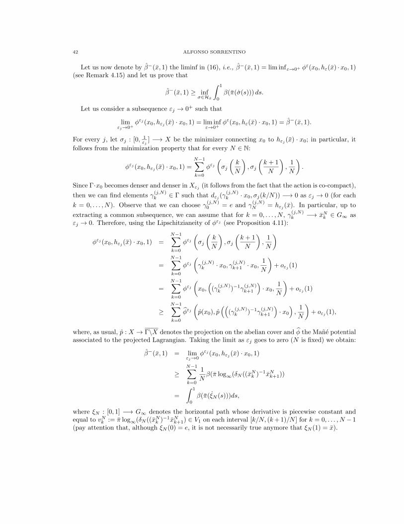
42 ALFONSO SORRENTINO
Let us now denote by β−(x, 1) the liminf in (16), i.e., β−(x, 1) = lim infε→0+ φε(x0, hε(x) ·x0, 1)(see Remark 4.15) and let us prove that
β−(x, 1) ≥ infσ∈Hx
∫ 1
0
β(π(σ(s))) ds.
Let us consider a subsequence εj → 0+ such that
limεj→0+
φεj (x0, hεj (x) · x0, 1) = lim infε→0+
φε(x0, hε(x) · x0, 1) = β−(x, 1).
For every j, let σj : [0, 1εj
] −→ X be the minimizer connecting x0 to hεj (x) · x0; in particular, it
follows from the minimization property that for every N ∈ N:
φεj (x0, hεj (x) · x0, 1) =
N−1∑k=0
φεj(σj
(k
N
), σj
(k + 1
N
),
1
N
).
Since Γ·x0 becomes denser and denser in Xεj (it follows from the fact that the action is co-compact),
then we can find elements γ(j,N)k ∈ Γ such that dεj (γ
(j,N)k · x0, σj(k/N)) −→ 0 as εj → 0 (for each
k = 0, . . . , N). Observe that we can choose γ(j,N)0 = e and γ
(j,N)N = hεj (x). In particular, up to
extracting a common subsequence, we can assume that for k = 0, . . . , N , γ(j,N)k −→ xNk ∈ G∞ as
εj → 0. Therefore, using the Lipschitzianeity of φεj (see Proposition 4.11):
φεj (x0, hεj (x) · x0, 1) =
N−1∑k=0
φεj(σj
(k
N
), σj
(k + 1
N
),
1
N
)
=
N−1∑k=0
φεj(γ
(j,N)k · x0, γ
(j,N)k+1 · x0,
1
N
)+ oεj (1)
=
N−1∑k=0
φεj(x0,(
(γ(j,N)k )−1γ
(j,N)k+1
)· x0,
1
N
)+ oεj (1)
≥N−1∑k=0
φεj(p(x0), p
(((γ
(j,N)k )−1γ
(j,N)k+1
)· x0
),
1
N
)+ oεj (1),
where, as usual, p : X → Γ\X denotes the projection on the abelian cover and φ the Mane potentialassociated to the projected Lagrangian. Taking the limit as εj goes to zero (N is fixed) we obtain:
β−(x, 1) = limεj→0
φεj (x0, hεj (x) · x0, 1)
≥N−1∑k=0
1
Nβ(π log∞(δN ((xNk )−1xNk+1))
=
∫ 1
0
β(π(ξN (s)))ds,
where ξN : [0, 1] −→ G∞ denotes the horizontal path whose derivative is piecewise constant andequal to vNk := π log∞(δN ((xNk )−1xNk+1) ∈ V1 on each interval [k/N, (k+ 1)/N ] for k = 0, . . . , N − 1(pay attention that, although ξN (0) = e, it is not necessarily true anymore that ξN (1) = x).

HOMOGENIZATION OF THE HAMILTON-JACOBI EQUATION 43
Observe that since the norm of the velocities of the minimizers σj are equibounded (let us de-
note by A a possible upper-bound), then dεj (γ(j,N)k · x0, γ
(j,N)k+1 · x0) ≤ A
N + oεj (1) and therefore
εjdΓ(γ(j,N)k , γ
(j,N)k+1 ) ≤ B
N + oεj (1), for some positive constant B (which may differ from A, if dΓ is
not the orbit metric). Hence, d∞(e, δN ((xNk )−1xNk+1)) ≤ B for k = 0, . . . , N .We can then apply [6, Lemma 1.5 and Lemma 3.2] and deduce that d∞(ξN (1), x) = O(1/N). Hence:
β−(x, 1) ≥∫ 1
0
β(π(ξN (s)))ds ≥ infσ∈Hx
∫ 1
0
β(π(σ(s))) ds+O(1/N).
The claim follows by taking the limit as N → +∞. And this concludes the proof.
4.6. Convergence of Rescaled Solutions and Proof of the Main Theorem. We want toshow now that the rescaled solutions vε(·, ·) of (9) – see formula (10) – converge uniformly oncompact sets (in the sense of Definition 4.9) to
v(x, T ) = infy∈G∞
f(y) + β
(y−1x, T
)= inf
y∈G∞
f(y) + TL
(δ1/T (y−1x)
),
where the second equality follows from Proposition 4.13.
Remark 4.21. It has been proven in [2, Theorem 3.4] that such a v is the unique viscosity solutionto the following problem:
∂tv(x, t) +H(∇Hv(x, t)) = 0 (x, t) ∈ G∞ × (0, T )v(x, 0) = f(x) x ∈ G∞,
where H : g∞[g∞,g∞] −→ R is the convex conjugate of β restricted to the subspace π(g∞) '
H1(Γ\X;R) (observe that without assuming H1(X;R) = 0, π(g∞) might be a proper subspaceof H1(Γ\X;R)). In particular, modulo identifying H1(Γ\X;R) with g∞
[g∞,g∞] , we can conclude that
H coincides with Mather’ α-function, analogously to what happens in [30, 14].
Let us start by proving the following Lemma (see also [14, Lemma 3.3]).
Lemma 4.22. Given a compact set K ⊂ G∞ and a compact interval J ⊂ (0,+∞), there exists apositive constant C > 0 such that for sufficiently small ε > 0:
dε(hε(x) · x0, yε) ≤ C
for any x ∈ K, T ∈ J and yε ∈ X realizing the minimum in the definition of vε(hε(x) · x0, T ).

44 ALFONSO SORRENTINO
Proof. Since f : G∞ → R is assumed to have at most linear growth, i.e.,
supx∈G∞
|f(x)|1 + d∞(e, x)
<∞,
then there exist A,B > 0 such that:
f(x) ≥ −Ad∞(e, x)−B.
Since fε are assumed to converge locally uniformly to f (see Definition 4.9), if x is in a compactset K ⊂ G∞, then for ε sufficiently small we have that fε(hε(x) · x0) ≤ Q, for some Q > 0, and
fε(hε(x) · x0) ≥ f(x)− 1
≥ −Ad∞(e, x)− (B + 1).(23)
Recall now that L is superlinear, therefore for any M > 0 there exists N = N(M) > 0 such that,taken any pair x, y ∈ X and a curve γ linking them in time T , then:
(24)
∫ T
0
L(γ, εγ)dt ≥M dε(x, y)−NT.
Moreover, from the definition of vε:
vε(hε(x) · x0, T ) := inf
fε(γ(0)) +
∫ T
0
Lε(γ(t), γ(t)) dt∣∣ γ ∈ C1([0, T ], X), γ(T ) = hε(x) · x0
.
Then, if follows easily that for ε small, if x ∈ K and T ∈ J then (let us denote MJ := maxT∈J T ):
vε(hε(x) · x0, T ) ≤ Q+MJ maxy∈X|L(y, 0)| ≤ Q1.(25)
Let yε be a point achieving the infimum in vε(hε(x) · x0, T ) for some x ∈ K and T ∈ J . Then,using that fε are equiLipschitz (with constant Λ), the estimate in (24) with M sufficiently large (itsuffices to take M > Λ) and (23), we obtain:
vε(hε(x) · x0, T ) ≥ fε(yε) +M dε(hε(x) · x0, yε)−NT≥ fε(hε(x) · x0) + (M − Λ)dε(hε(x) · x0, yε)−NT≥ −Ad∞(e, x)− (B + 1) + (M − Λ)dε(hε(x) · x0, yε)−NMJ
≥ M1dε(hε(x) · x0, yε)−N1,
where M1 := M − Λ and N1 := A diam∞(K) + B + 1 + NMJ . Using this estimate and (25), wecan conclude that:
dε(hε(x) · x0, yε) ≤ 1
M1(A1 +Q1) =: C = C(J,K).

HOMOGENIZATION OF THE HAMILTON-JACOBI EQUATION 45
4.6.1. Proof of the Main Theorem. We can now prove the Main Theorem (see statement in subsec-tion 1.1.8). Observe that once we have proved the convergence of vε to v as ε goes to zero (part i)),then the proof will be essentially complete: part ii), in fact, follows from Proposition 4.17, whilepart iii) follows from Remark 4.21.
Proof. [Main Theorem] Let us consider a point (x, T ) in G∞ × (0,+∞); the sequence δε(hε(x))converges to x with respect to the metric Q (see Remark 4.8 ii)).
• Let us first prove the pointwise convergence, i.e.,
limε→0+
vε(hε(x) · x0, T ) = v(x, T ).
Assume that vεk(hεk(x) · x0, T ) is a subsequence converging to the liminf and let us denote by yεkthe corresponding points at which the infimum (minimum) in the definition of vεk(hεk(x) · x0, T )is achieved. Let us denote by γεk a sequence of elements of Γ such that εkd(γεk · x0, yεk) → 0 asεk goes to zero (this is possible, since the set Γ · x0 becomes denser and denser, with respect tothe distance dεk). According to Lemma 4.22, dεk(hεk(x) · x0, yεk) < C for εk small, so this means
that (at least for εk small) δεk(γεk) lie in a compact set (see Remark 4.8 ii)) and therefore – up to
possibly extracting a subsequence – we can assume that δεkγεk converges to some y ∈ G∞ (in thesense of Remark 4.8 ii)).
In particular, δεk(γ−1εkhεk(x)
)converges to y−1x and
limεk→0+
φεk(γεk · x0, hεk(x) · x0, T ) = limεk→0+
φεk(x0,(γ−1εkhεk(x)
)· x0, T )
= limεk→0+
φεk(x0, hεk(y−1x) · x0, T )
= β(y−1x, T ).
Moreover,
|fεk(yεk)− fεk(γεk · x0)| ≤ εkK1d(yεk , γεk · x0) −→ 0
and
|φεk(yεk , hεk(x) · x0, T )− φεk(γεk · x0, hεk(x) · x0, T )| ≤ εkK2d(yεk , γεk · x0) −→ 0.
Therefore,
limεk→0
vεk(hεk(x) · x0) = limεk→0
(fεk(yεk) + φεk(yεk , hεk(x) · x0, T ))
= limεk→0
(fεk(γεk · x0) + φεk(γεk · x0, hεk(x) · x0, T ))
= f(y) + limεk→0
φεk(γεk · x0, hεk(x) · x0, T )
= f(y) + β(y−1x, T ) ≥ v(x, T ).
Therefore,
(26) lim infε→0+
vε(hε(x) · x0) ≥ v(x, T ).

46 ALFONSO SORRENTINO
Let now y be the optimal element in the definition of v(·, T ) (it does exist since L is convex andsuperlinear) and consider the sequence hε(y).Then:
vε(hε(x) · x0, T ) ≤ fε(hε(y) · x0) + φε(hε(y) · x0, hε(x) · x0, T ).
Taking the limit as ε goes to zero we obtain:
lim supε→0+
vε(hε(x) · x0, T ) ≤ lim supε→0+
(fε(hε(y) · x0) + φε(hε(y) · x0, hε(x) · x0, T ))
≤ f(y) + limε→0+
φε(x0, (hε(y)−1hε(x)) · x0, T )
= f(y) + β(y−1x, T ) = v(x, T ).
This and (26) allow us to conclude that for each T > 0 and x ∈ G∞ we have
limε→0+
vε(hε(x) · x0, T ) = v(x, T ).
• Let now xε → x in (G∞, d∞) and Tε → T . Then, using the equiLipschitzianity of the vε (seeProposition 4.4, observing that for T in a compact set of (0,+∞) the Lipschitz constant can bechosen uniformly, at least for small ε):
|vε(hε(xε) · x0, Tε)− v(x, T )| ≤ |vε(hε(xε) · x0, Tε)− vε(hε(x) · x0, Tε)|+ |vε(hε(x) · x0, Tε)− vε(hε(x) · x0, T )|+ |vε(hε(x) · x0, T )− v(x, T )|
≤ K1dε(hε(xε) · x0, hε(x) · x0) +K2|Tε − T |+ |vε(hε(x) · x0, T )− v(x, T )|
≤ K3d∞(xε, x) +K2|Tε − T |+ |vε(hε(x) · x0, T )− v(x, T )|,
which goes to zero as ε goes to zero. Hence:
(27) limε→0+
vε(hε(xε) · x0, Tε) = v(x, T ).
• Let us now prove that this convergence is uniform for x in compact sets of G∞ and T in a compactinterval J ⊂ (0,+∞), i.e.,
limε→0+
supB∞(R)×J
|vε(hε(x) · x0, T ))− v(x, T )| = 0.
If by contraddiction this were not true, then we could find a sequence εk → 0, elements (xk, Tk) ∈B∞(R)× J and δ > 0, such that
(28) |vεk(hεk(xk) · x0, Tk)− v(xk, Tk)| > δ ∀ k.
Up to extracting a subsequence, we could assume that xk → x ∈ B∞(R) and Tk → T > 0, andit would follow from (27) that
limεk→0
vεk(hεk(xk), Tk) = v(x, T ),
which clearly contradicts (28). Therefore, the convergence must be uniform.

HOMOGENIZATION OF THE HAMILTON-JACOBI EQUATION 47
Remark 4.23. It follows from the proof that v is Lipschitz on compact subsets of G∞ × (0,+∞),hence continuous.
References
[1] Vladimir I. Arnol′d. Mathematical methods of classical mechanics. Graduate Texts in Mathematics 60, Springer-
Verlag, New York, pp. xvi + 516, 1989.[2] Z. M. Balogh, A. Calogero and R. Pini. The Hopf-Lax formula in Carnot groups: a control theoretic approach.
Calc. Var. Partial Differential Equations 49 (3-4): 13791414, 2014.
[3] Guy Barles. Solutions de viscosite des equations de Hamilton-Jacobi. Mathematiques & Applications 17: x+194pp., Springer Verlag, 1994.
[4] Hyman Bass. The degree of polynomial growth of finitely generated nilpotent groups. Proc. London Math. Soc.
25 (3): 603–614, 1972.[5] Stanley H. Jr. Benton. The Hamilton-Jacobi equation. A global approach. Mathematics in Science and Engi-
neering, Vol. 131. Academic Press, New York-London, pp. xi+147 , 1977.
[6] Emmanuel Breuillard and Enrico Le Donne. Nilpotent groups, asymptotics cones and subfinsler geometry.Preprint, 2012.
[7] Dmitri Burago, Yuri Burago and Sergei Ivanov. A course in metric geometry. Graduate Studies in Mathematics,
Vol. 33, American Mathematical Society, 2001.[8] Mario J. Dias Carneiro. On minimizing measures of the action of autonomous Lagrangians.. Nonlinearity 8 (6):
1077–1085, 1995.[9] Kai Cieliebak, Urs Frauenfelder and Gabriel P. Paternain. Symplectic topology of Mane critical values. Geom.
Topol., 14 (3): 1765–1870, 2010
[10] Michael G. Crandall and Pierre-Louis Lions. Viscosity solutions of Hamilton-Jacobi equations. Transactions ofthe AMS 277 (1): 1–42, 1983.
[11] Michael G. Crandall and Pierre-Louis Lions. On existence and uniqueness of solutions to Hamilton-Jacobi
equations. Nonlinear Anal. 10 (4): 353–370, 1986.[12] Gonzalo Contreras. Action potential and weak KAM solutions. Cal. Var. Part. Diff. Eq. 13 (4): 427– 458, 2001.
[13] Gonzalo Contreras and Renato Iturriaga. Global minimizers of Autonomous Lagrangian systems. 22th Coloquio
Bras. Mat., IMPA, Rio de Janeiro, 1999.[14] Gonzalo Contreras, Renato Iturriaga and Antonio Siconolfi. Homogenization on arbitrary manifolds. Cal. Var.
Part. Diff. Eq. 52 (1-2): 237–252, 2015.
[15] Gonzalo Contreras and Gabriel P. Paternain. Connecting orbits between static classes for generic Lagrangiansystems. Topology 41 (4): 645–666, 2002.
[16] Richard Courant and David Hilbert. Methods of mathematical physics, Vol. II. Wiley Classics Library, John
Wiley & Sons, Inc., New York, pp. xxii+830, 1989.[17] L. van den Dries and A. J. Wilkie. Gromov’s theorem on groups of polinomial growth and elementary logic. J.
Algebra 89 (2): 349–374, 1984.[18] Vadim A. Efremovic. On proximity geometry of Riemannian manifolds. Uspekhi Math. Nauk 8 189–191, 1953
(Russian). English translation: Amer. Math. Soc. Transl. (2) 39: 167–170, 1964.
[19] Lawrence C. Evans. The perturbed test function method for viscosity solutions to nonlinear PDE. Proceedingsof the Royal Society of Edinburgh, 111 A: 359–375, 1989.
[20] Lawrence C. Evans. Weak KAM theory and partial differential equations. Calculus of variations and nonlinearpartial differential equations, 123–154, Lecture Notes in Math., 1927, Springer, Berlin, 2008.
[21] Lawrence C. Evans. Partial differential equations. Second edition. Graduate Studies in Mathematics, 19, Amer-ican Mathematical Society, xxii+749 pp., 2010.
[22] Albert Fathi. Orbites heteroclines et ensemble te Peierls. C. R. Acad. Sci. Paris Ser. I Math. 326 (10): 1213–126, 1998.
[23] Albert Fathi. Weak KAM Theorem in Lagrangian Dynamics. Preliminary version number 10, 2008. Undercontract with Cambridge University Press.
[24] Albert Fathi and Ezequiel Maderna. Weak KAM theorem on non compact manifolds. NoDEA 14: 1–27, 2007.[25] Herbert Federer and Wendell H. Fleming. Normal and integral currents. Ann. of Math. 72: 458–520, 1960.[26] Mikhael Gromov. Groups of polinomial growth and expanding maps. Publ. Math. IHES 53: 53–73, 1981.
[27] Hitoshi Ishii. Remarks on existence of viscosity solutions to Hamilton-Jacobi equations. Bull. Fac. Sci. Eng.
Chuo Univ. 26: 5–24, 1983.

48 ALFONSO SORRENTINO
[28] Bruce Kleiner. A new proof of Gromov’s theorem on groups of polynomial growth. J. Amer. Math. Soc. 23 (3):815–829, 2010.
[29] Pierre-Louis Lions. Generalized solutions to Hamilton-Jacobi equations. Research Notes in Mathematics 69,
Pitman, iv+317 pp, 1982.[30] Pierre-Louis Lions, Georgios Papanicolaou and S. R. Srinivasa Varadhan. Homogeneization of Hamilton-Jacobi
equations. Preprint, 1987.[31] Anatoly I. Malcev. On a class of homogeneous spaces. Isvestiya 13: 9–32, 1949 (Russian). English translation:
Amer. Math. Soc. Trans. 39, 1951.
[32] Ricardo Mane. Lagrangian flows: the dynamics of globally minimizing orbits. Bol. Soc. Brasil. Mat. (N.S.) 28(2): 141–153, 1997.
[33] John N. Mather. Action minimizing invariant measures for positive definite Lagrangian systems. Math. Z. 207:
169–207, 1991.[34] John N. Mather. Variational construction of connecting orbits. Ann. Inst. Fourier (Grenoble), 43 (5): 1349-1386,
1993.
[35] Richard Montgomery. A tour of subriemannian geometries, their geodesics and applications. Mathematical Sur-veys and Monographs, Vol. 91, American Mathematical Society, Providence, RI, 2002.
[36] Alezandra Monzner, Nicolas Vichery and Frol Zapolsky. Partial quasi-morphisms and quasi-states on cotangent
bundles and symplectic homogenization. Journal of Modern Dynamic 6 (2): 205–249, 2012.[37] Pierre Pansu. Croissance des boules et des geodesiques fermees dans les nilvarietes. Ergodic Theory Dynam.
Systemes, 3(3): 415–445, 1983.
[38] Gabriel P. Paternain, Leonid Polterovich and Karl F. Siburg. Boundary rigidity for Lagrangian submanifolds,non–removable intersections, and Aubry-Mather theory. Mosc. Math. J., 3 (2): 593–619, 2003.
[39] M. S. Raghunathan. Discrete subgroups of Lie groups. Ergebnisse der Mathematik und ihrer Grenzgebiete, Band68, Springer-Verlag, New York, 1972.
[40] Mark Sapir. Asymptotic cones of groups. Lecture notes from a mini-course at CRM, Universite de Montreal,
August 2010.[41] Alfonso Sorrentino. Action-minimizing methods in Hamiltonian dynamics: an introduction to Aubry-Mather
theory. Mathematical Notes Vol. 50, Princeton and Oxford University Press, pp. xi + 128, May 2015.
[42] Alfonso Sorrentino and Gabriel P. Paternain. Symplectic and contact properties of the Man?e critical value of
the universal cover. To appear on NoDEA: Nonlinear Differ. Equ. Appl., 2014.[43] Simon Thomas and Boban Velickovic. Asymptotic cones of finitely generated groups. Bull. London Math. Soc.
32 (2): 203–208, 2000.
[44] Claude Viterbo. Symplectic Homogenization. Preprint, 2014.[45] Joseph A. Wolf. Growth of finitely generated solvable groups and curvature of riemannian manifolds. J. Diff.
Geom. 2: 421–446, 1968.
E-mail address: [email protected]
Dipartimento di Matematica, Universita degli Studi di Roma “Tor Vergata”, Viale della Ricerca
Scientifica 1, 00133 Rome (Italy).