homogenization of metric hamilton-jacobi...

HOMOGENIZATION OF METRIC HAMILTON-JACOBIEQUATIONS

ADAM M. OBERMAN, RYO TAKEI, AND ALEXANDER VLADIMIRSKY

Abstract. In this work we provide a novel approach to homogeniza-tion for a class of static Hamilton-Jacobi (HJ) equations, which we callmetric HJ equations. We relate the solutions of the HJ equations tothe distance function in a corresponding Riemannian or Finslerian met-ric. The metric approach allows us to conclude that the homogenizedequation also induces a metric. The advantage of the method is that wecan solve just one auxiliary equation to recover the homogenized Hamil-tonian H(p). This is significant improvement over existing methodswhich require the solution of the cell problem (or a variational problem)for each value of p. Computational results are presented and comparedwith analytic results when available for piece-wise constant periodic andrandom speed functions.

Contents

1. Introduction 21.1. Particle speeds and front normal velocities 31.2. The periodic checkerboard 51.3. The random checkerboard 51.4. The toy three scale problem 62. Paths and fronts in an inhomogeneous medium 72.1. Summary of notation and relationship between the variables 82.2. The speed function, vectograms 82.3. The arrival time function 92.4. The Hamilton-Jacobi equation 92.5. The Lagrangian 102.6. Special cases: isotropic and homogeneous speeds 102.7. The geodesic distance 112.8. Relating the geodesic metric and the arrival time 122.9. Dual Norms, the Eikonal equation 133. Homogenization 14

Date: June 7, 2009.2000 Mathematics Subject Classification. 49L25, 60G40, 35B27.Key words and phrases. partial differential equations, Hamilton-Jacobi, homogeniza-

tion, geodesic, metric, front propagation.The second author was supported in part by ONR grant N00014-03-1-0071. The third

author was supported in part by the NSF grant DMS-0514487.

1

2 ADAM M. OBERMAN, RYO TAKEI, AND ALEXANDER VLADIMIRSKY

3.1. Homogenization background 143.2. Homogenization in one dimension 143.3. The cell problem for Hamilton-Jacobi equations 153.4. Variational formulation for fronts 153.5. Homogenization of metrics 163.6. Main Homogenization Result 164. The Numerical Method 194.1. Computing the homogenized speed function 204.2. Numerical Solution of the HJ equation 204.3. ENO interpolation of vectograms 214.4. Solving the homogenized equation on a coarse grid 224.5. A graph-based discretization of Ω. 225. Numerical Results 245.1. Homogenized speed functions 245.2. The toy three scale problem 255.3. Methods and parameters used 265.4. Cell and domain resolutions 285.5. Front propagation in random media 296. Conclusions 30References 31

1. Introductionsec:intro

In this work we provide a novel approach to homogenization for a class ofconvex Hamilton-Jacobi (HJ) equations, which we call metric HJ equations.We relate the solutions of the HJ equations to the distance function in acorresponding Riemannian or Finslerian metric. By appealing to a homog-enization result for metrics, we conclude that the homogenized equation isalso the distance in a homogenized metric. The advantage of our methodis that we can solve just one auxiliary equation to recover the homogenizedHamiltonian H(p). This is significant improvement over existing methodswhich require the solution of the cell problem (or a variational problem) foreach value of p.

An application is front propagation problems in multiscale media. Thewide range of spatial scales prohibits the direct solution of the fully re-solved problem. However the separation of scales allows homogenization:the medium which varies on small scales is replaced by a homogeneousmedium, which approximates the propagation of the fronts on the largerscale.

The main theoretical idea is to recognize that the distance function in thehomogenized metric captures the solution to a variational problem for thegeodesics corresponding to all directions. This distance function, which isapproximated by solving a single Hamilton-Jacobi equation, can be used torecover the entire homogenized metric. To make this procedure work, we

HOMOGENIZATION OF METRIC HAMILTON-JACOBI EQUATIONS 3

need to be able to easily translate results for anisotropic front propagationbetween various formulations (reviewed in section §2). The first formulationexpresses the speed of propagation in the media by a local speed function.The speed function induces a metric on the space, given by the least timeto traverse using admissible paths. The distance function in this metricsatisfies an eikonal-type Hamilton-Jacobi equation.

Remark. Our results apply to the metric Hamiltonian H(p, x) = 1, definedbelow, which homogenizes to H(p). We mention here that the results ex-tend to some other cases, provided H(p, x) is a metric Hamiltonian. Whileit is not completely obvious, it is true that H2(∇u, x) = 1 homogenizes toH2(∇u) = 1. In the time-dependent case, ut = H(∇u, x), homogenizes tout = H(∇u). In addition, ut = H2(∇u, x) homogenizes to ut = H2(∇u).These results can be obtained using the Hopf-Lax formula. For an explana-tion, see the remarks at the end of section §2.9 and at the start of section §3.

Another natural definition of metric in an inhomogeneous medium is pro-vided by the geodesic distance. In this case a cost function is minimized.over admissible paths (which are not required to have bounded speeds). Therelationship between the cost function and the speed function which makesthe geodesic metric equal to the metric induces by the speed function isgiven in §2.8.

In our approach, we compute an approximation to the homogenized La-grangian L(q) for all values of q. The Legendre transform is then appliedto obtain H(p) for all values of p. In fact, it is often more convenient tosolve anisotropic Hamilton-Jacobi equations by semi-Lagrangian numericalmethods. In that case, all that is needed is L(q), and the additional step ofapplying Legendre transform can be avoided.

Contents. The remainder of this section introduces anisotropic front prop-agation, and presents a few model problems. Section §2 reviews front prop-agation more thoroughly. The HJ equation for the arrival time is derived,and the geodesic distance is presented. The Lagrangian and the Hopf-Laxformula are reviewed. Section §3 contains a review of homogenization andthe proof of the main theoretical result. The algorithmic details of our nu-merical method are provided in section §4, and the numerical results can befound in section §5.

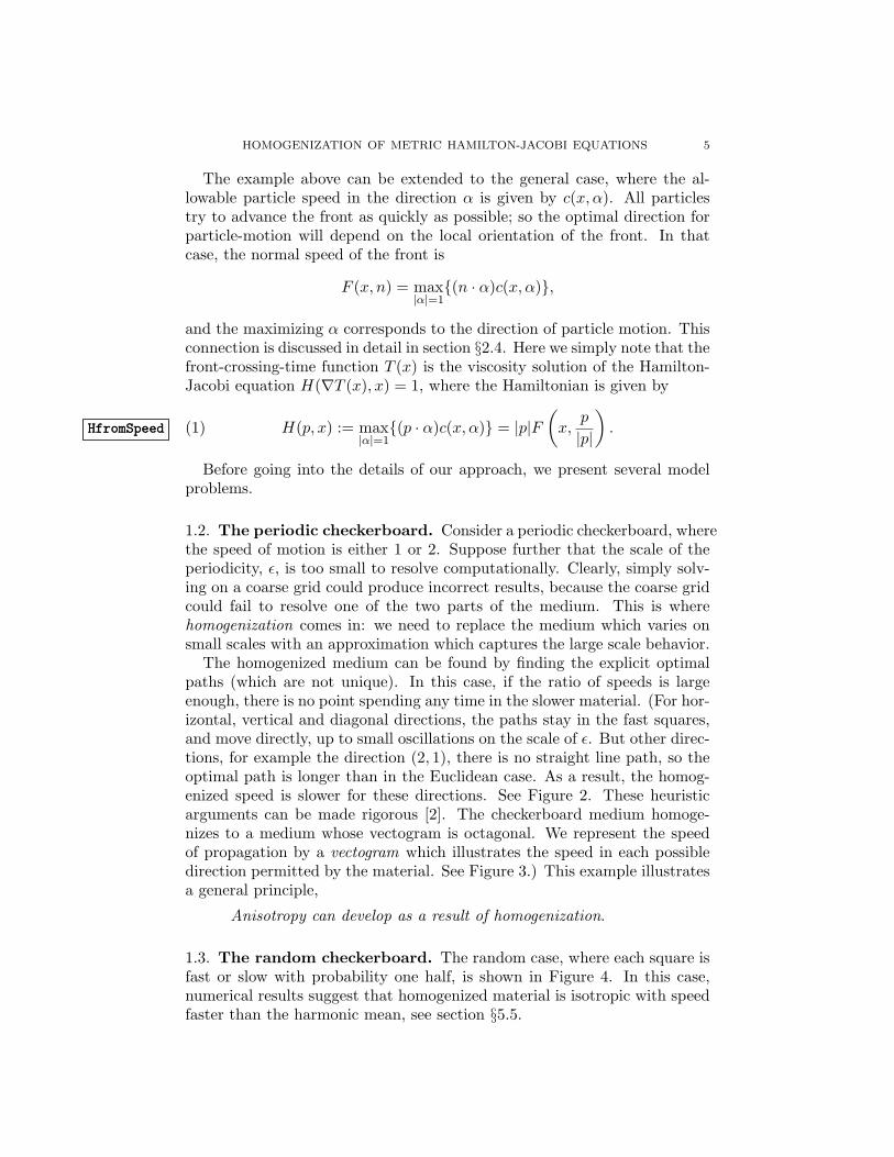
1.1. Particle speeds and front normal velocities. Suppose Γ is theinitial position of a front which is advancing monotonically, passing througheach point only once. In this case the position of the front at time t canbe represented by the level set of a single function T (x). If T (x) is thetime when the front passes through the point x, then the level-sets of Tgive subsequent positions of the front. Assume that the normal speed of thefront, F (x, n), depends only on the position, x, and normal direction, n. Ifthe front remains smooth, its normal direction is n = ∇T

|∇T | and the rate ofincrease of T in that direction is equal to |∇T |. On the other hand, this rate


n

v

v

v vn

Figure 1: Illustration of normal front speed versus particle speed. fig:front

of increase should be the reciprocal of the normal speed, F . This yields thefollowing static Hamilton-Jacobi equation

F

(x,∇T (x)|∇T (x)|

)|∇T (x)| = 1

with the boundary condition T = 0 on Γ. However, this argument is formal,since the advancing front will generally not remain smooth. (For two grow-ing circles, the front develops a cusp when they intersect.) To deal withsingularities, the notion of viscosity solutions should be used to interpretthis Partial Differential Equation (PDE) [15].

A Lagrangian formulation of the same problem results from consideringa front as an aggregate of infinitely many particles, all of which are movingalong optimal trajectories, with the goal of advancing in the front’s normaldirection as quickly as possible. The optimal particle trajectories coincidewith the characteristics of the above PDE, and the front remains smooth aslong as these optimal trajectories do not intersect.

In order to properly link the Hamilton-Jacobi equation with the La-grangian formulation, we need to be particularly careful when dealing withanisotropic speeds. In the isotropic case, F (x, n) = c(x) and the opti-mal direction for particle-travel is also orthogonal to the front, yielding theEikonal PDE

c(x)|∇T (x)| = 1.

In the anisotropic case, the normal velocity of the front is different from thevelocity of the moving particles which make up that front.

Example. Suppose particles move horizontally with speed 1, and have novertical speed allowed. Then the front with normal (1, 1)/

√2 moves with

speed 1/√

2 in the normal direction, whereas the vertical front moves atspeed 1 and a horizontal front does not move at all. See Figure 1.


The example above can be extended to the general case, where the al-lowable particle speed in the direction α is given by c(x, α). All particlestry to advance the front as quickly as possible; so the optimal direction forparticle-motion will depend on the local orientation of the front. In thatcase, the normal speed of the front is

F (x, n) = max|α|=1(n · α)c(x, α),

and the maximizing α corresponds to the direction of particle motion. Thisconnection is discussed in detail in section §2.4. Here we simply note that thefront-crossing-time function T (x) is the viscosity solution of the Hamilton-Jacobi equation H(∇T (x), x) = 1, where the Hamiltonian is given by

HfromSpeedHfromSpeed (1) H(p, x) := max|α|=1(p · α)c(x, α) = |p|F

(x,

p

|p|

).

Before going into the details of our approach, we present several modelproblems.

1.2. The periodic checkerboard. Consider a periodic checkerboard, wherethe speed of motion is either 1 or 2. Suppose further that the scale of theperiodicity, ε, is too small to resolve computationally. Clearly, simply solv-ing on a coarse grid could produce incorrect results, because the coarse gridcould fail to resolve one of the two parts of the medium. This is wherehomogenization comes in: we need to replace the medium which varies onsmall scales with an approximation which captures the large scale behavior.

The homogenized medium can be found by finding the explicit optimalpaths (which are not unique). In this case, if the ratio of speeds is largeenough, there is no point spending any time in the slower material. (For hor-izontal, vertical and diagonal directions, the paths stay in the fast squares,and move directly, up to small oscillations on the scale of ε. But other direc-tions, for example the direction (2, 1), there is no straight line path, so theoptimal path is longer than in the Euclidean case. As a result, the homog-enized speed is slower for these directions. See Figure 2. These heuristicarguments can be made rigorous [2]. The checkerboard medium homoge-nizes to a medium whose vectogram is octagonal. We represent the speedof propagation by a vectogram which illustrates the speed in each possibledirection permitted by the material. See Figure 3.) This example illustratesa general principle,

Anisotropy can develop as a result of homogenization.

1.3. The random checkerboard. The random case, where each square isfast or slow with probability one half, is shown in Figure 4. In this case,numerical results suggest that homogenized material is isotropic with speedfaster than the harmonic mean, see section §5.5.


Figure 2: An optimal path in the (2, 1) direction for the checkerboard ma-terial.

fig:path

Figure 3: Homogenization of the checkerboard material, illustrated withvectograms.

fig:checkerboard

toy3scale1.4. The toy three scale problem. Consider a two dimensional materialmade up of fifty by fifty unit blocks. Each block is allowed to have a differentperiodic small scale structure. See Figure 5.

To solve the full three scale problem, we apply a two step procedure.First in each block, homogenize to get a homogenous material with a new(anisotropic) speed profile. Next, on the large scale, solve the front propaga-tion problem on a grid which resolves each block, using the speed profile forthe homogenized blocks. See Figure 5 and Figure 11. Accurate results canbe obtained with a modest number of grid points on each block, see §5.2.


Figure 4: Optimal paths in a random media. The particle speed is c0 > 1in the dark and 1 in the light region. Left: c0 = 2. Right: c0 = 10.

fig:randomPath

Figure 5: The three scale problem (left), result of homogenization in eachmedium scale cell (right)

fig:3scaleSol

2. Paths and fronts in an inhomogeneous mediumsec:fronts

In this section we review front propagation in an inhomogeneous andanisotropic medium from the perspective of the optimal control theory. We


discuss the least time perspective, and the related Eikonal equation for thedistance.

We recall the derivation of the Hamilton-Jacobi equation for the distancefunction. The distance function is interpreted as the first arrival time fora front given as the envelope of particles moving along the optimal pathsat speed given by c. The normal speed of a front is not the same as theparticle speed. However, we make the observation in 2.9 that the particlespeed function defines a norm, and that the HJ equation for the distance isa generalized eikonal equation in the dual norm.

These different interpretations of HJ equations are later used in section §3to derive an efficient method for homogenization.

sec:summary2.1. Summary of notation and relationship between the variables.• x is a generic point in Rn representing position.• p, q are generic vectors in Rn representing velocity.• β is a generic vector in Rn satisfying |β| ≤ 1.• α is a generic unit vector in Rn representing direction.• c(x, α) is the particle speed in the direction α.• f(x, α) gives the particle velocity in the direction α, f(x, α) = αc(x, α)• F (x, n) gives the speed for a front with normal n.• b(x, q) is the cost at x to move with velocity q.• The vectogram, Vc(x) = f(x, β) | |β| ≤ 1 is a set of all permissible

velocities at the point x.• The Hamiltonian, H(p, x) = |p|F (x, p/|p|).• The Lagrangian L(q, x) = 0 if q ∈ Vc(x), ∞ otherwise.

The normal speed F and particle speed c are related by the homogeneousLegendre Transform [31]. The Hamiltonian, H, and the Lagrangian L arerelated by the Legendre Transform, see section §2.5. The particle speed c andthe metric cost function b are one sided inverse functions, see section §2.8.For each fixed x, the metric cost function b and the Hamiltonian H arenorms on Rn. These are dual norm, see section §2.9.

2.2. The speed function, vectograms. Consider a medium which allowsparticle motion at limited speeds. Let x denote the position, and β denotethe control value. Write x(s, β(s)) := d

dsx(s, β(s)). The admissible pathsx(s, β(s)) satisfy the controlled ordinary differential equation

dynamicsdynamics (ODE) x(s, β(s)) = f(x(s, β(s)), β(s)),

where β(·) ∈ B := β(·) : [0,∞)→ Rn, |β| ≤ 1, measurable is the control.We restrict to the special case where the control is the choice of direction:

speedfunctionspeedfunction (2) f(x, β(s)) = c

(x,

β(s)|β(s)|

)β(s).

The speed function c : Rn × Sn−1 → [0,+∞) gives the maximum speedallowed in the direction α, where α = β(s)|β(s)|−1 is a unit vector. We


assume that c is convex in its second argument and satisfies the small-timecontrollability condition:

growthgrowth (3) 0 < c1 ≤ c(x, α) ≤ C1 < +∞ for every x ∈ Rn, |α| = 1.

The function c is homogeneous if it is independent of x, c(x, α) = c(α),isotropic if it is independent of the direction, α, c(x, α) = c(x), and sym-metric if

speedsymmetricspeedsymmetric (4) c(x,−α) = c(x, α).

We assume symmetry to ensure that the resulting distances on Rn, Tc(x1, x2),are symmetric, although the assumption can be dropped at the expense ofsome additional bookkeeping (we would need to distinguish between arrivaltimes, and times to reach a target, some of the formulas will have minus signsin the velocities, see [31] and norms are replaced by asymmetric norms).

For fixed x ∈ Rn, the speed function c is a mapping of the unit sphere,Sn, and also defines a vectogram Vc ⊂ Rn:

Vc =c(x, β|β|−1

)β∣∣ |β| ≤ 1

.

Vectograms [23] provide a simple way to illustrate the speed profile for eachpoint x. See Figures 3 and 8.

sec:arrivaltime2.3. The arrival time function. We can define a distance on Rn usingthe minimum time needed to move between two points along the admissiblepaths:

dsds (5) Tc(x1, x2) = infx(·) admissible

t | x(0) = x1, x(t) = x2.

It is easy to show that Tc defines a metric on Rn, where the symmetryproperty results from the fact that any admissible path from x1 to x2 can beretraced backwards taking the same amount of time (using (4)). The small-time controllability condition (3) can be used to show that the infimum isattained and that an optimal (not necessarily unique) control β(s) actuallyexists. Moreover, since the goal is to minimize the time, it is clear thatalong any optimal path the particle should be moving with the maximumallowable speed for the current direction; i.e., |β(s)| = 1 and f(x(s), β(s)) ison the boundary of the vectogram Vc a.e. in [0, t]. Thus, the same distancefunction can be defined by using the class of admissible controls A := α(·) :[0,∞)→ Rn, |α| = 1, measurable.

sec:dist2.4. The Hamilton-Jacobi equation. In this section we show directlythat the first arrival time function satisfies the Hamilton-Jacobi equation,using the Dynamic Programming Principle [5]. Here we give a formal proof(assuming the solution remains smooth), for the reader’s convenience, and toestablish consistent notation. A rigorous treatment (using visosity solutionsto handle the non-smoothness) as well as the proof of uniqueness for similarequations can be found in [18] and [5].


lem:1 Property 1. The arrival time to the origin, T (x) = Tc(x, 0), is the viscositysolution to the Hamilton-Jacobi equation

hjbhjb (HJ) H(∇T, x) = 1, T (0) = 0,

where the Hamiltonian H(p, x) is given by (1).

Proof. Assume that T (x) is smooth and consider all paths, which start fromx and move in the constant direction α for a small time h. Define yα =x+ hc(x, α)α. Then

T (x) = minαT (yα) + h+ o(h2)

= minαT (x) + c(x, α) (α · ∇T (x)) + h+ o(h2).

Subtracting T (x), dividing by h, and taking the limit h→ 0 gives

−1 = minαc(x, α) (α · ∇T (x)),

or max|α|=1c(x,−α) (α · ∇T (x)) = 1 as in (1), where we have used thesymmetry of the speed (4).

sec:Lagrangian2.5. The Lagrangian. An equivalent way to define the distance, (5), isusing the Lagrangian,

LagDefLagDef (6) L(q, x) =

0 q ∈ Vc,∞ otherwise.

Then the definition of distance (5) can be rewritten as the Hopf-Lax for-mula [18] for the arrival time function

HopfLaxHopfLax (7) T (x) = inft+∫ t

0L(x(s), x(s)) ds

∣∣∣∣ x(0) = 0, x(t) = x

,

where the infimum is over W 1,1 ((0, t); Rn). For consistency, we verify thatthe Hamiltonian H(p, x) is obtained from the Lagrangian via the Legendretransformation [18]

H(p, x) = L∗(p, x) = maxqp · q − L(q, x)

= maxq∈Vc

p · q

= max|α|=1(p · α) c(x, α).

2.6. Special cases: isotropic and homogeneous speeds. The optimalparticle trajectories are given by the characteristics of the Hamilton-Jacobiequation. In the anisotropic case, the normal speed F (x, n) is given by (1),

F (x, n) = max|α|=1(n · α) c(x,−α).


When c(x, α) = c(x) is isotropic, then F (x, n) = c(x). and H(p, x) =|p|c(x) = 1, which is an Eikonal equation. In this case, the characteristiccurves coincide with the gradient lines of the viscosity solution, yielding

n =∇T (x)|∇T (x)|

.

On the other hand, in the special case where the speed function is homo-geneous, c(x, α) = c(α), the optimal paths are straight lines, and the arrivaltime to a point is simply given by the ratio of the distance to the speed.

TimeHomogTimeHomog (8) T (x) =|x|

c(x/|x|), when T (0) = 0 and c(x, α) = c(α)

For the more general boundary condition T (x) = g(x) on Γ, we obtain

homogenized_from_Gammahomogenized_from_Gamma (9) T (x) = miny∈Γ

|x− y|

c(x−y|x−y|

) + g(y)

.

sec:geodesic2.7. The geodesic distance. We review the notion of geodesic distancein this context, and below we will relate it to Hamilton-Jacobi equations.The link between Hamilton-Jacobi equations and metrics has been observedbefore. We refer to [32] and the references therein.

We are given a metric cost function, b(x, q) which is positively 1-homogeneousin the second variable,

1homogfc1homogfc (10) b(x, tq) = tb(x, q), for every (x, q) ∈ Rn × Rn and t > 0.

This will ensure that the distance defined below is invariant under changeof parameterizations of the path. In addition, we assume that b is convex inthe second variable and satisfies the growth condition:

growthfcgrowthfc (11) c2|q| ≤ b(x, q) ≤ C2|q|, for every (x, q) ∈ Rn × Rn,

with 0 < c2 ≤ C2 < +∞. Under the assumptions (10) and (11), the costfunction defines a norm on Rn, for each x,

FcnormFcnorm (12) ‖q‖b = b(x, q).

We also assume that b(x, q) = b(x,−q), which ensures the distance is sym-metric, db(x1, x2) = db(x2, x1).

Given a path x(·) ∈W 1,1 ((0, t); Rn), the total cost of the path is

JdefnJdefn (13) J [x(·)] =∫ t

0b (x(s), x(s)) ds.

The geodesic distance between two points is the minimal cost

geodesicgeodesic (14) db(x1, x2) = inf J [x(·)] | x(0) = x1, x(t) = x2

where the infimum is over x(·) ∈W 1,1 ((0, t); Rn).


Remark (Riemannian and Finslerian metrics). If the cost function is givenby the square root of a convex quadratic function, i.e.

b(x, α) =√gij(x)αiαj ,

for g(x) a symmetric positive definite matrix, the resulting metric, db, isRiemannian. (In that case the vectograms Vc are ellipses.) Otherwise, db isa Finslerian metric [32].

Remark (Non-differentiable geodesics). In a Finslerian metric, geodesicsneed not be differentiable, as is the case for the octagon norm. See [12][4]for more information on Finslerian metrics. The distance function may alsobe non-differentiable.

sec:relating

2.8. Relating the geodesic metric and the arrival time. So far wehave defined two distances. The arrival time, Tc(x1, x2), (5), is the arrivaltime using paths which move at speed admissible by the speed functionc(x, α). The geodesic distance, db(x1, x2), (14) is the minimal cost of paths,where the cost is measured using the metric cost function b(x, p). The twodistances are equal if the metric cost function and the particle speed functionare (one-sided) inverses.

lem:2 Lemma 1. The distances defined by (5) and (14), respectively, are equal,

distequaldistequal (15) Tc(x1, x2) = db(x1, x2),

provided that the speed function, c, and the cost function, b, are related by

fcdefnfcdefn (16) b(x, c(x, α)α) = 1, for all |α| = 1, x ∈ Rn,

with the remaining values of b determined by homogeneity (10).

Proof. We argue formally, assuming the infimum in the definitions is achievedby differentiable paths. The proof can be made rigorous by approximation.Given x1, x2 ∈ Rn, suppose Tc(x1, x2) = t and db(x1, x2) = s.

First letx(·) : [0, t]→ Rn, x(0) = x0, x(t) = x1.

be an admissible curve for the speed function c. Then x(·) satisfies (ODE),and Tc(x0, x1) = t. Compute the integral in the definition (14) using thepath x(·). Then by (ODE), x(s) ∈ Vc. Furthermore, we can assume thatx(s) ∈ ∂Vc, since otherwise the curve could be made faster. Thus by (16),b(x, x) = 1, so s ≤ t.

Next let x(·) be a curve from x1 to x2 for which the cost J [x(·)] = s. Wecan find a parameterization of the path by arclength, i.e. a path y(·), forwhich b(y(s), y(s)) = 1. Then by (16), y(s) ∈ Vc, the vectogram at y(s), soy(·) is an admissible path for the distance function Tc. Thus t ≤ s.

A similar proof of this property can be also found in [33].


sec:dualnorm2.9. Dual Norms, the Eikonal equation. We recall that (HJ) can berewritten as an Eikonal equation in a suitable (x-dependent) norm. Thisrelates the speed or cost functions to the normal velocity.

We refer to [7][ Appendix 1.1.6] for material on norms and dual norms. Aclosed, bounded set with non-empty interior, e.g. Vc, can be used to definea norm (by using the set as the norm ball and extending by homogeneity)provided the set is symmetric about the origin, and convex. Convexity ofthe set ensures the triangle inequality for the norm.

Given a norm ‖ · ‖ on Rn, the dual norm ‖ · ‖∗ is defined as

dualnormdualnorm (17) ‖x‖∗ = maxx · y | ‖y‖ = 1.

Then ‖x‖∗∗ = ‖x‖.

Example. The p-norms ‖x‖p = (∑n

i=1 |x|p)1/p are dual to the q norms, with1/p + 1/q = 1 for 1 ≤ p ≤ ∞. This follows from Holder’s inequality onRn, x · y ≤ ‖x‖p‖y‖q. In particular this is true for p = 1 and p = ∞,where the norm balls are diamonds and squares. Generalizing this case, dualpolygonal norms can be obtained as well. For example, the dual of the norm‖x‖ = max(|x1|, |x2|, |x1 + x2|), is the norm ‖x‖∗ = max(|x1|, |x2|, |x1 − x2|)

Write, for fixed x, the dual norm

‖p‖b∗ := maxp · q | ‖q‖b = 1= max|q|=1p · q c(x, p).

by (16). Thus equation (1) is equivalent to

H(∇T (x), x) = ‖∇T (x)‖b∗.

If we are given the Hamilton-Jacobi equation H(p, x) which is positive1-homogeneous in p for each x, we can recover the cost function by takingthe dual

fcfromHfcfromH (18) ‖q‖b = maxpq · p | H(p, x) = 1.

The Legendre transform of the norm ‖·‖b∗ is the dual norm unit ball [7][pg 93],which gives the vectogram.

Remark. In general it is not true that homogenizing and squaring commute,by which we mean that if the Hamiltonian S(p, x) = H2(p, x) it may notbe the case that S(p) = H(p)2, even assuming both homogenize. However,if H(p, x) is a metric Hamiltonian, then that last formula does hold. Thisresult can be seen by using the variational interpretation, and noting thatthe Legendre transform of a norm is the indicator set of the dual norm, whilethe Legendre transform of a norm squared is the dual norm squared (see [7]example 3.26 and 3.27). Thus the results of [13] (for eikonal squared) and[14] (for eikonal) can be translated from one to the other.


3. Homogenizationsec:homog

We provide an overview of prior homogenization results and different vari-ational perspectives in Sections 3.1-3.5. Combining these different interpre-tations and the Hopf-Lax formula (8), we derive Theorem 1 in Section 3.6.This theorem serves as a basis for the efficient numerical methods describedin Section 4.

sec:31

3.1. Homogenization background. Theoretical works on homogeniza-tion provide existence results and convergence rates for the solution of thehomogenization problem. We mention the early unpublished work [25] forHamilton-Jacobi equations, and refer to the textbooks, [26] for linear equa-tions, and [8], for homogenization of HJ equations and Riemannian metrics[pp142–145]. A list of more detailed references can be found in the review [17]

Variational interpretations for the homogenization problem, and a seriesof explicit analytic solutions can be found in [13] and in [14]. Both worksfind explicit solutions by homogenizing the Lagrangian, refer to sections §3.4and §2.5. The first work used Hamiltonians which are homogeneous ordertwo in p, (H(p, x)2 in our notation), and so the resulting Lagrangian wasalso homogeneous order two in p. The second work used a time-dependentequation, with a similar Hamiltonian to the one herein. In both cases, theLagrangian is related to the Hamiltonian by the Legendre transform.

The cell problem (section §3.3) can be solved numerically to computeH(p). This was done for front propagation in [24] and [11], and for moregeneral Hamiltonians in [27] and [28]. There are other methods for com-puting H(P ), see [19]. Theoretical justification for some of the numericalapproaches can be found in [1, 9].

3.2. Homogenization in one dimension.

Example. For the case of front propagation in a one-dimensional periodicmedium, it is not difficult to show that the homogenized speed function isthe harmonic mean of the speed function over a periodic cell. Suppose ourone dimensional domain consists of ε-intervals with the speed alternatingbetween 1 and 5. Then the travel times in these materials are 1 and 1/5,so the total time for the front to traverse the entire domain is 3/5, and theaverage speed is 5/3, the harmonic mean of 1 and 5.

To obtain this result formally for the Hamilton-Jacobi equation, we gothrough the following procedure. (i) rewrite c(x)|Tx| = 1, as |Tx| = c(x)−1,(ii) average the reciprocal of the speed function (iii) divide by the averagedcoefficient, to obtain

1average of c(x)−1

|Tx| = 1.

Remark. This heuristic is quite similar to the one used when homogenizinglinear equations, but it is not directly applicable to HJ equations in higherdimensions. To obtain the total cost to travel from x0 to x1 the cost is


integrated along the optimal trajectory, (which need not be a straight line).The homogenized cost for that direction is then obtained by dividing thetotal cost by |x0− x1|. The cost has units of inverse speed, the average costis the time divided by the distance.

sec:cell3.3. The cell problem for Hamilton-Jacobi equations. In this sectionwe outline the cell problem. A precise statement of a typical theorem canbe found, for example, in [10], or in the review [17]. The cell problem isderived using a formal asymptotic expansion, typical examples of which canbe found in Chapter 5 of [21].

Let H (p, x) be a Hamiltonian with is periodic on the cube [−1, 1)n. LetT ε(x) be the solution of

H(∇T ε(x),

x

ε

)= 1

with T ε(0) = 0. We are interested in the limit ε → 0. Formally expandthe solution, T ε, in ε, T (x) = T 0(x, x/ε) + εT 1(x, x/ε) + O(ε2). Additionalarguments which we skip show that we can assume

T ε(x) = T 0(x) + εT 1(x/ε) +O(ε2).

Inserting the expansion into the equation, and collecting terms of O(1) gives

H(∇xT 0 +∇yT 1, y

)= 1,

where y = x/ε. The variable in this last equation is y, so ∇xT 0 = p, anunknown constant. The left hand side of the previous equation is a functionof y, while the right hand side is constant. Thus we have a solvabilitycondition: we need to find a periodic function v(y), and a vector p whichsolve the cell problem

H(p+∇v, x) = 1.

Then we can defineH(p) = 1,

for that particular value p, and extend H to other values along the lineq = tp by homogeneity. According to the theorem, T ε converges (uniformlyon compact subsets) to the solution of

H(∇T ) = 1.sec:var_fronts

3.4. Variational formulation for fronts. For time-dependent fronts, avariational formulation of the homogenization problem was used in [14]. Thisis based on the Lagrangian formulation of the problem, and the convergenceis in the sense of Γ-convergence [8]. The variational problem takes the form

L(q) = lim infT→∞

1T

infφ∈H1

0 (0,T )

∫ T

0L(qt+ φ(t), q + φ(t)) dt.


In this case, the minimization is performed for each value of q, and theHamiltonian H(p) is recovered via the Legendre transform. The result-ing Hamiltonian is homogeneous of order one in the gradient, and the La-grangian is a characteristic function, as in (6). We note that the discon-tinuous nature of the Lagrangian limits the usefulness of this approach fornumerical approximation.

sec:homogmetric3.5. Homogenization of metrics. In this section, we review a homoge-nization result for the geodesic distance functional.

We use the result from [3]. Consider the metric cost functional (13).In addition to (10) and (11), in this section we also assume that b(·, q) is[−1, 1)n periodic for every q ∈ Rn. Then for every ε > 0, set

J ε[x(·)] =∫ t

0b

(x(s)ε, x(s)

)ds,

According to the theorem from [3], Jε Γ-converges on W 1,1 ((0, t); Rn) (inthe L1-topology) to the function defined by

J [x(·)] =∫ t

0b(x(s)) ds.

Here b : Rn → [0,+∞) is 1-homogeneous convex function which also satis-fies (11) and is given by

barfbarf (19) b(q) = limε→0+

infx(·)

∫ t

0b

(x(s)ε, x(s)

)ds | x(0) = 0, x(t) = q

,

where again the infimum is over x(·) ∈W 1,1 ((0, t); Rn).sec:36

3.6. Main Homogenization Result. It is too costly to use the formula (19)which requires the solution of a path minimization problem for each direc-tion q. However, if we knew the homogenized Hamiltonian, we could readit off from the solution of the equation for the first arrival time to the ori-gin (HJ). But we can approximate this solution by the solution of theinhomogeneous small ε equation (HJ ε). This results in an efficient methodfor H(p) We record this result in Theorem 1. See Figure 6 for an illustrationof the result, taken from a computation.

Definition 1. The Hamiltonian H(p, x) : Rn×Rn → R is a metric or gener-alized eikonal Hamiltonian if for each fixed x, H(·, x) : Rn → R satisfies thefollowing

H(·, x) is convex

H(tp, x) = tH(p, x) for all t ≥ 0

c2|p| ≤ H(p, x) ≤ C2|p|

with 0 < c2 ≤ C2 < +∞.


Figure 6: The arrival time T ε(x) using the periodic cost function b(x/ε, p)converges to the arrival time T (x) with the homogenized cost b(p).

fig:cones

Remark. The next theorem begins by collecting different formulations ofthe Hamiltonian. The metric formulations allows us to avoid solving a cellproblem for each value p. Instead, equation (22) can be used to solve only onehigh resolution problem, from which the entire homogenization Hamiltoniancan be recovered.

thm:HJ Theorem 1. Let H(p, x) be a metric Hamiltonian which is periodic on theunit hypercube. Then

H(p, x) = max|α|=1(p · α)c(x, α) = ‖p‖b∗

where c(x, α) is the particle speed, b(x, p) is the metric cost function, andthe subscript ∗ indicates the dual norm.

The viscosity solutions T ε(x) of the Hamilton-Jacobi equation

HJeHJe (HJ ε)

H(∇T ε(x), xε

)= 1,

T ε(0) = 0,

converge uniformly on compact subsets to the viscosity solution T (x) of

HJbHJb (HJ)

H(∇T (x)) = 1,T (0) = 0.

H(p) is also a metric Hamiltonian, given by

HJbarHJbar (20) H(p) = max‖α‖=1

(p · α)c(α) = ‖p‖b∗


where c(α), b are the homogenized speed and cost functions, respectively.These functions can be obtained from the arrival time function in the ho-mogenized metric

fcbarfcbar (21) b(q) =1c(q)

=T (q)|q|

,

and are approximated by

raterate (22) b(q) =1c(q)

=T ε(q)|q|

+O(ε),

where T ε is the solution of (HJ ε).

Remark (Convergence rate). The formal analysis used to obtain the conver-gence rate (22) gives the error as a power series in ε, c1ε+O(ε2). This lastfact, which we do not address here, allows the use of Richardson extrapola-tion in ε to better approximate T (x).

This result is obtained from translating freely between the various for-mulations of the front propagation problems, as summarized in §2.1 and asexplained in the earlier sections.

Proof. We begin with the definition of H in terms of the particle speed (1)

H(p, x) := max‖α‖=1

(p · α)c(x, α).

Since H(p, x) is a metric Hamiltonian, we can recover the cost functionb(x, p) from the Hamiltonian using the dual norm formula (18)

b(x, q) = ‖q‖b = maxpq · p | H(p, x) = 1.

By Property 1, the solution T ε(x) of the Hamilton-Jacobi equation (HJ ε)is the arrival time from the origin using admissible speeds cε, given by (5)

T ε(x) = infx(·)t | x(0) = 0, x(t) = x, x(·) admissible for cε(x, α) .

Using Lemma 1 in Section §2.8, this is equal to the distance in the bε metric,

T ε(x) = infx(·)

∫ t

0bε (x(s), x(s)) ds

∣∣∣∣ x(0) = 0, x(t) = x

,

for x(·) ∈W 1,1 ((0, t); Rn).At this stage, we appeal to the convergence result for metrics, [3], which

is summarized in Section §3.5. The functionals, J ε, Γ-converge to the ho-mogenized cost functional, J . The cost function, bε(x, q), converges to acost function, b(q), which is also homogeneous of order one. The mini-mizing paths xε(·) are minimizers of the functionals, and converge in theL1-topology to the minimizer of the homogenized functional. The distancesin the metric T ε(x) are the minimum values of the functional for paths fromthe origin to the point x. The values T ε(x) converge (in R) to T (x) over theminimizing sequences xε as ε→ 0.


Again using Lemma 1, we can write the distance, T (x), in the homog-enized metric b as the solution of the Hamilton-Jacobi equation for thehomogenized cost (20), which gives the last equality in (20),

H(p) = ‖p‖b∗.

If we know H(p), we can recover the speed function from the cost functionusing (18) (actually the formula for the inverse), giving the second equalityin (20),

H(p) = max‖α‖=1

(p · α)c(α).

Since these functions are convex, the optimal path is a straight line, inthe directions α = x/|x|. Then the travel time for a particle is simply thedistance over the particle speed (8)

cbareqcbareq (23) T (x) =|x|

c(x/|x|)which gives the second equality in (21).

The convergence of metrics result is useful because it ensures that the His also a metric Hamiltonian. However, to obtain the convergence rate (22),we appeal to results which apply in the more general context of homog-enization of period Hamilton-Jacobi equations. We can apply the resultof [10], if we transform our equation using the Kruzkov transformation:T ε(x) = − log(1− vε(x)). The result is the convergence rate (22),

T (x) = T ε(x) +O(ε).

Remark. We note that the variational interpretations of the homogenizationprocess have been previously used in [13] and[14]. Moreover, the formula forhomogenizing b has been recognized as a convenient building block for ex-pressing H(p) (see, for example, formula (3.2) in [14]). However, the noveltyof our approach is based on observing that b can be efficiently approximatedfor all q’s simultaneously by solving a single PDE, thus making the ap-proximation of H(p) for multiple directions p much less computationallyexpensive.

4. The Numerical Methodsec:numerical_method

In this section we present our numerical method for homogenization. Forthe sake of notational simplicity, the method is described in two dimensions,but the generalization to higher dimensional problems is straightforward.

The first step of our algorithm solves (HJ ε) to obtain an approxima-tion to the homogenized speed and cost functions, c(α), b(q), using (22)in Theorem 1, see sections 4.1 and 4.3. If we are only interested in solv-ing (HJ), then the solution is provided by (23). If instead, we want to solveH(∇T ) = 1 with general boundary conditions, then the solution can berecovered from (9), or it can be obtained numerically. While the analyticalformula is useful for evaluating the solution at one point, it is more efficient


to solve the equation numerically on a coarse grid, see section 4.4, if thevalues of the solution on a domain are required.

By combining multiscale problems with different homogenized Hamilto-nians in different regions, we solve a toy three scale problem in §5.2, withminor modifications of the method outlined in section §4.4.

To summarize, the complete algorithm consists of two steps: the first isto compute the homogenized speed function c(α) for all unit vectors α onthe small scale, and the second is to use the homogenized speed function tosolve numerically for T (x) on the large scale.

sec:homog_speed_numerics4.1. Computing the homogenized speed function. Our plan for com-puting c(α) is based on the formula (21) in §3.

• INPUT: speed function cε(x, α).• OUTPUT: c(α), the approximation to the homogenized speed in the

direction α.

(A1) Choose 0 < h ε 1. Numerically solve (HJ ε) on a uniformcartesian grid on Q = [−1, 1]2 with spatial resolution h.

(A2) Choose k vectors qiki=1, which lie on the grid and are of lengthclose to unity, and whose directions αi = qi

|qi| are nearly equallydistributed on the circle. Approximate c on the grid directions,using (21)

c (αi) :=|qi|

T ε(qi), i = 1, ..., k.

(A3) Interpolate the values c(αi)ki=1 to approximate c(α) for all direc-tions α.

4.2. Numerical Solution of the HJ equation. Equation (HJ ε) can besolved by standard methods. In the isotropic case, cε(x, α) = cε(x), the PDEis Eikonal, which makes both Fast Marching [30] and Fast Sweeping [34]methods directly applicable. A computational comparison of fast marchingand fast sweeping approaches to Eikonal PDEs can be found in [22, 20].

Since the discretization of (HJ ε) uses a relatively fine grid, the com-putational efficiency of the method used to obtain the discretized solutionis important. The Fast Marching Method computes the numerical solu-tion in O(M logM) operations, where the total number of gridpoints isM = O(h−n), in Rn, regardless of how oscillatory cε(x) is. On the otherhand, the number of sweeps needed in the fast sweeping method is propor-tional to the number of times the characteristics switch their direction fromquadrant to quadrant. As a result, the highly oscillatory nature of cε(x)mean that the Fast Sweeping Method will require many more sweeps thanin the constant cε case.

In the more general case where cε is anisotropic, the step (A1) can becarried out using Ordered Upwind Methods [31].


sec:ENO4.3. ENO interpolation of vectograms. We use a second-order essen-tially non-oscillatory (ENO) method for interpolation. The ENO methodcan exactly interpolate piecewise quadratic functions. This class matches theshape of the vectograms corresponding to the homogenized speed functions.See Figure 7. In particular, since it can capture vectograms with corners,the ENO method is suitable for approximating not only Riemannian, butalso general (Finslerian) metrics.

−1 0 1

−1

−0.5

0

0.5

1

−1 0 1

−1

−0.5

0

0.5

1

−1 0 1

−1

−0.5

0

0.5

1

−1 −0.5 0 0.5 1

−1

−0.5

0

0.5

1

Figure 7: Interpolation using ENO. Interpolated circle, using 8, 16, and 24points. Interpolated octagon using 16 points.

fig:ENOcircle

The second order ENO method works as follows. Order the unit vectorsαi in the counter-clockwise direction. Interpolate c(αi)αi between i = jand j + 1 as follows. Write

c(αi)αi = (xi, yi)

We describe the case where xi is the independent variable, which shouldbe applied where |xj − xj+1| is not too small. The case where yi is theindependent variable follows similarly, where |yj − yj+1| is not too small.

Step 1 Find the interpolating quadratics

h1(x) = a1x2 + a2x+ a3, h1(xi) = yi, i = j − 1, j, j + 1,

h2(x) = b1x2 + b2x+ b3, h2(xi) = yi, i = j, j + 1, j + 2.

Step 2 If |a1| < |b1|, choose h1(α) as the interpolating function betweenc(αj)αj and c(αj+1)αj+1. Otherwise, choose h2(α) as the interpo-lating function.

Remark. We interpolate in Cartesian coordinates, not polar coordinates,even though the latter appears simpler. This method has the special advan-tage that it captures piecewise linear vectograms exactly, which the polarcoordinate version does not.

Remark. The method is more accurate for anisotropy which is aligned alongthe grid directions. More interpolation points along more grid directionscan be added when this is not the case.


sec:coarse_grid_numerics

4.4. Solving the homogenized equation on a coarse grid. The ho-mogenized PDE can be written as

H(∇T ) = max|α|=1(α · ∇T )c(α) = 1.

Given c, formula (8) provides the solution of this PDE on Ω with the bound-ary condition T (0) = 0. As was stated earlier, the solution of H(∇T ) = 1with general boundary conditions can be recovered from (9). However, agood approximation to T (x) can be obtained more efficiently by solving thisPDE numerically on a coarse grid in Ω.

Remark. The availability of c(α) makes semi-Lagrangian discretizations ofthe homogenized Hamilton-Jacobi PDE particularly attractive. (Any Euler-ian discretization would require an extra step of approximating the dualnorm to b.) Fast non-iterative methods are available for many semi-Lagran-gian discretizations. If a finite list of directions of motion is well-representedon a large-scale grid, this results in an auxiliary grid-based graph with pos-itive edge-weights. As a result, the shortest path problem can be solved onthat graph using a non-iterative Dijkstra’s methods, section §4.5. A moreaccurate semi-Lagrangian discretization, spanning all possible directions oflarge-scale motion, was also shown to posses similar causal properties, re-sulting in related non-iterative Ordered Upwind Methods described in [31].

sec:Dijkstra4.5. A graph-based discretization of Ω. We implement a discrete ana-logue of the dynamic programming principle, where the optimal path isapproximated by piecewise linear paths on a finite set of nodes in Ω. Weembed a network X in Ω consisting of a finite node set V ⊂ Ω and weighteddirected edges E ⊂ V × V . For each x ∈ V , the neighbors of x form the set

N (x) = y ∈ V : (x, y) ∈ E.We call the set

C(x) = y − x : y ∈ N (x),the local connectivity of X at x ∈ V . Construct X so that for all x, y ∈ V

y ∈ N (x)⇔ x ∈ N (y),

and generally,|v| is small for all v ∈ C(x), x ∈ V .

The latter condition allows for more accurate approximation of the optimaltrajectories (and consequently of the value function) by piecewise linearpaths. Naturally, the metric between two adjacent nodes are assigned asthe (directed) edge weights. The shortest path problem on a network canthen be efficiently solved using Dijkstra’s method [16] or by a variant of aFast Sweeping Method.• INPUT: c(α) from phase one of the algorithm.• OUTPUT: T , the discrete approximation to the T (x) defined on V .


(B1) For each ei = (x, y) ∈ E assign a positive edge weight

wi = w(x, y) = |y − x|/c(y − x|y − x|

).

(B2) Initialize:

T 0(x) =

g(x) if x ∈ V ∩ Γ,∞ if x ∈ V \Γ.

(B3) Use either Dijkstra’s algorithm or the Fast Sweeping Method tocompute the value function T (x) (i.e., the least cost to travel fromV ∩ Γ to a node x using the edges in E) for all x ∈ V \Γ.

The value function satisfies the following system of discretized equations

value_funcvalue_func (24) T (x) = maxy∈N (x)

w(x, y) + T (y)

, ∀x ∈ V \Γ.

If M = |V \Γ| and k = max |N (x)|, Dijkstra’s method solves this system inO(kM logM) operations.

Choice of grid directions qi and network X. Using Dijkstra’s algorithm(B1) - (B3) to approximate the value function, step (A3) may be omittedby carefully choosing the grid directions qi (in (A2)) and network X.

For example, consider the network where the vertices V are given byuniform cartesian discretization of Ω with refinement h, and for each interiornode, the neighbors are the eight closest nodes,

C = C(x) = (±h, 0), (±h,±h), (0,±h).Then by choosing the grid directions

qi = vi/h where vi ∈ C, i = 1, . . . , 8,

in the step (A2), we can avoid the interpolation step (A3), since the valuesat the grid directions are the only values needed to compute the weights in(B1).

However, this introduces an additional error, because the paths used forcomputing the metric in (19) are being restricted to those which are piece-wise linear with slopes corresponding to the grid directions. This error canbe reduced by using more grid directions.

Alternatively, the use of a more accurate semi-Lagrangian discretizationdescribed in [31] will automatically minimize over all possible directions ofmotion, but with that approach the step (A3) becomes unavoidable.

Extension to piecewise-periodic problems. Our algorithm generalizes natu-rally to problems with multiple regions, each with different periodic struc-ture. Suppose Ω =

⋃ki=1 Ωi is a (finite) partition of the domain, where each

Ωi is equipped with a speed function cεi(x, α). By repeating (A1) - (A3) ineach domain, we approximate ci(α) for each i. Define the piecewise constant(in x) speed function on Ω by

c(x, α) = ci(α), x ∈ Ωi.


Then proceed as before with the weights assigned as in (B1) using the glob-ally defined speed function c(x, α). A numerical example of this kind isconsidered in §5.2.

Remark. In the periodic medium, the characteristics of the homogenizedPDE will be straight lines. In the piecewise-periodic case, the effectiveHamiltonian is discontinuous, and the characteristics might change the di-rection upon crossing the boundary between Ωi and Ωj . Nevertheless, for areasonably small number of subdomains k, the fast sweeping approach willbe even more efficient than Dijkstra’s method here, since the characteristicsrarely switch direction from quadrant to quadrant.

5. Numerical Resultssec:numericalresults

Numerical results and validation are presented in this section. We presenthomogenization results in several cases where an analytic solution is known.The methods and parameters used in our implementation are described. Wenumerically validate the first order convergence in ε. Finally, we present aresult for the three scale problem.

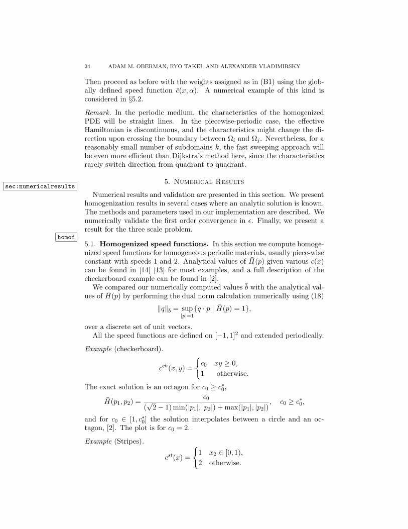
homof5.1. Homogenized speed functions. In this section we compute homoge-nized speed functions for homogeneous periodic materials, usually piece-wiseconstant with speeds 1 and 2. Analytical values of H(p) given various c(x)can be found in [14] [13] for most examples, and a full description of thecheckerboard example can be found in [2].

We compared our numerically computed values b with the analytical val-ues of H(p) by performing the dual norm calculation numerically using (18)

‖q‖b = sup|p|=1q · p | H(p) = 1,

over a discrete set of unit vectors.All the speed functions are defined on [−1, 1]2 and extended periodically.

Example (checkerboard).

cch(x, y) =

c0 xy ≥ 0,1 otherwise.

The exact solution is an octagon for c0 ≥ c∗0,

H(p1, p2) =c0

(√

2− 1) min(|p1|, |p2|) + max(|p1|, |p2|), c0 ≥ c∗0,

and for c0 ∈ [1, c∗0] the solution interpolates between a circle and an oc-tagon, [2]. The plot is for c0 = 2.

Example (Stripes).

cst(x) =

1 x2 ∈ [0, 1),2 otherwise.


The exact solution for general stripes pattern can be found in [14]. Weexplain a simple heuristic for computing the cost in this case. The totalcost for crossing a large number of stripes is the same even if the pattern isrearranged so that all the slow parts come first and the fast parts second.Then, given a path with slope m, the optimal path will have a corner atthe interface and slopes m1,m2 in the slow and fast parts, respectively. Theoptimal path for this configuration can be found by solving for the optimalslopes, which results in Snell’s law of refraction.

Example (Squares).

csq(x) =

1 x1 = 0 or x2 = 0,1/2 otherwise.

The exact solution is readily seen to be given by a diamond shaped vec-togram, since the optimal paths move only in the vertical and horizontaldirections.

circle Example (Circles).

ccir(x) =

1 ‖x‖ ≤ 1,2 otherwise.

The exact solution is in [13] [14],

H(p1, p2) = max|p1|, |p2|,

2π

(|p1|+ |p2|).

The optimal paths are made of segments which are either vertical lines,horizontal lines, or quarter circles.

The numerically computed homogenized vectograms are shown in Figure8, overlaid on the exact result. We also compared the error for a fixed pattern(checkerboard or stripes) but different speed ratios c in the material. Theerror was computed for a fixed directions as a function of c, and also as afunction of the direction for fixed c. See Figures 9 and 10.

sec:toy3scale_results5.2. The toy three scale problem. In this section we consider the modelproblem from §1.4. Consider the following speed function:

c(x) =

cch(x) for x ∈ [−1,−1

3 ]2 ∪ [−13 ,

13 ]2 ∪ [1

3 , 1]2,cst(x) for x ∈ [−1,−1

3 ]× [−13 ,

13 ] ∪ [−1

3 ,13 ]× [1

3 , 1],cvert(x) for x ∈ [−1

3 ,13 ]× [−1,−1

3 ] ∪ [13 , 1]× [−1

3 ,13 ],

csq(x) otherwise.

where cvert is the horizontal stripes cst rotated by 90 degrees. We solve foru0(x) in (HJ ε), in [−1, 1]2 with starting point (−0.7,−0.7). The numericallycomputed homogenized value function is shown in Figure 11.


Figure 8: Period domains and computed vectograms: checkerboard, stripes,squares, and circles.

fig:vectograms

1 2 3 4 5

0.997

0.9975

0.998

0.9985

0.999

0.9995

1

c

f 0(α), α

= (1

,1)

ComputedExact

1 2 3 4 5

3.22

3.23

3.24

3.25

3.26

3.27x 10−3

c

max

sam

pled

erro

r

Figure 9: Results using the checkerboard pattern for speeds in ∈ [1, 5]. Left:c(α) for α = (1, 1). Right: maximum error over all sampled directions.

fig:varyChecker

5.3. Methods and parameters used. We used the first order Fast March-ing Method to solve the boundary value problem (HJ ε) for grid size n =1200 and 2400 (so the refinements are h = 1/600 and 1/1200). Then weapplied Richardson’s extrapolation on h, the spatial resolution, to obtainsecond order accuracy. The grid directions qi were chosen to be the 24directions on a 7× 7 stencil, see Figure 12.

For the connectivity C of the network, first note that the weights fornodes on the edges of the 7× 7 stencil (marked by circles in Figure 12) areknown. Then, the weights for all other stencil nodes can be interpolatedalong the grid direction rays (the weight at the origin is zero), except fornodes not on the grid direction rays. Subsequently, for (B1) - (B3), the local


1 2 3 4 5

0.4

0.5

0.6

0.7

0.8

0.9

1

c

f 0(α), α

= (0

,1)

ExactComputed

1 2 3 4 51

2

3

4

5

6

7

8 x 10−6

c

max

sam

pled

erro

rFigure 10: Results using the horizontal stripes pattern for various speeds in[1, 5]. Left: c(α) for the direction α = (0, 1). Right: maximum error overall sampled directions.

fig:varyHorizontal

−1 −0.5 0 0.5 1−1

−0.8

−0.6

−0.4

−0.2

0

0.2

0.4

0.6

0.8

1

Figure 11: Level sets of the homogenized solution T (x). The dotted linesare the interfaces where the periodic pattern changes.

threeScaleProb

connectivities of the uniformly cartesian network X were chosen to be:

C = (ah, bh) : a, b ∈ 0,±1,±2,±3 − (ah, 2bh), (2ah, bh) : a, b ∈ ±1.The shortest path problem on X was computed using the Fast Sweeping

Method.The main script was written in Matlab, and the Fast Marching Method

was implemented in C, using code downloaded from [6]. The computations


Figure 12: The grid directions qi. fig:24direction

took a few seconds on a desktop computer. The default ratio of fast andslow speed in the cells was 2.

justifyextrap5.4. Cell and domain resolutions. In practice, computations were per-formed for finite values of ε. More accurate numerical results were obtainedby using Richardson extrapolation for two small values of ε. In this situa-tion, there is a trade off between the number of periodic cells on the domain,and the number of grid points in each cell.

We found that accurate results could be obtained by resolving each pe-riodic cell very well, even if a relatively small number of cells were used.Finally, we extrapolated in the spatial resolution h as well. Table 1 com-pares the errors resulting from different extrapolation choices. Extrapolationin both parameters yields the best accuracy.

Given n (n2 is the number of grid points used in step (A1).), and ε, definethe cell refinement by

nε := nε.

The accuracy of our algorithm depends on two parameters: ε and nε. Weobserved that the convergence rate depends more strongly on nε, than on ε.

extrapetable

pattern exactc(α)

error forh = ε/25, ε/50ε = 1/24

error forh = ε/25, ε/50ε = 1/12, 1/24

error forh = ε/100, ε/200ε = 1/3, 1/6

Checkerboard 1 -2.46E-02 -1.64E-02 -3.25E-03Squares 1/

√2 9.70E-04 9.65E-04 6.54E-05

Circles 0.90031 -5.10E-02 -4.74E-02 -1.70E-02Stripes 0.70051 -2.58E-03 -1.53E-02 -1.60E-06

Table 1: Errors in c(α) using extrapolation in: h only; h and ε (ε small); hand ε (ε large).


10−1 100

10−1

ε (log scale)

Erro

r (lo

g sc

ale)

nε = (20,40)

nε = (40,80)

nε = (80,160)

nε = (160,320)

O(ε)

Figure 13: Convergence rate in ε for various cell resolutions nε. circleepsiloninterp

Figure 13 shows the convergence rate as a function of ε of c(α) to theexact c(α). We used α = (cos(3π/4), sin(3π/4)) for the circle pattern §5.1.Similar results were observed for the other patterns.

In conclusion, the best accuracy is achieved when the two values of ε werechosen to be the two largest cell sizes such that the grid directions qi alllie on corners of periodic cells, and Richardson’s extrapolation is applied.When we used 24 directions, qi, the best choice was ε = 1/3 and 1/6.

sec:random_media_results5.5. Front propagation in random media. We now consider a randommedia example. Consider a random checkerboard structure, where in eachcell the speed

c(x) =

1 with probability 0.5,c0 > 1 with probability 0.5.

In this section, computations were performed using higher resolution, butplots use coarser computations for visualization purposes. Sample optimalpaths are shown in Figure 4 for two different values of c0, and with ε = 1/40.Experimentally, the homogenized speed c(α), averaged over several realiza-tions, is isotropic; the vectogram is a circle. Computations were performedaveraging over 20 trials, and sampling 24 sampled directions.

The mean and variance of c were computed, as a function of c0. In eachcase, the variance was less than 10−3. Figure 14 shows the averaged c(α)for ε = 0.01 on a 20002 grid (but plotted on an 802 grid) and the ENOinterpolated vectogram with 24 sampled directions, averaged over 20 trials.The dependence of c on the value c0 is also plotted, It was more informativeto plot b = 1/c as a function of 1/c0., see Figure 14.

Remark (Average cost in the random case). An upper bound for the homog-enized cost is the average of the costs in each cell. This is achieved by pathsmoving in a straight line in the direction α. But since optimal paths canwander to lower cost cells, the actual computed cost is lower. Better upper


bounds can be achieved by estimating the probability that a neighboring cellis low cost. We are not aware of any known formulas for the homogenizedspeed in this case.

−1 −0.5 0 0.5 1

−1

−0.5

0

0.5

1

random, α = 2

0 5 10 151

1.2

1.4

1.6

1.8

cost

1/(

mean r

adiu

s)

Figure 14: Illustration of the homogenized speed/cost in the random case.Left: computed vectogram, averaged over several trials, for c = 1, 1/2 withprobability 1/2. Right: computed homogenized cost b as a function of therandom cost b = 1, or b = b0 = 1/c0 with probability 1/2.

randomMV

randomConeCircle

6. Conclusions

We have introduced a new efficient method for approximating front prop-agation in periodic multi-scale media. Our approach is based on homog-enization of static convex Hamilton-Jacobi equations. We discuss the re-lationship between several interpretations of such PDEs (from front prop-agation to time-optimal control to geodesic distance computations). Theeffective Hamiltonian, resulting from the homogenization, is homogeneous.In more general settings it may vary slowly on the large scale. We includea brief overview of prior methods for homogenization based on solving thecell problem for each direction of front propagation. In contrast, our newtechnique uses a single auxiliary boundary value problem to approximatethe homogenized speed of particle motion for all directions. The methodtakes advantage of the special structure of the Hamiltonian, and the re-lationship to the Finsler metric, to compute the homogenized metric, andthen recover the homogenized Hamiltonian. The homogenized metric costfunction and the homogenized particle speed function are related to dualnorms, an equivalent way to relate front speeds and particle speeds is viathe homogeneous Legendre transform. The added advantage of is the easeof use of semi-Lagrangian numerical schemes on the large scales.

We have illustrated our method with a number of examples of periodic,piecewise-periodic and random checkerboards. All of these examples start


with an isotropic front propagation on the small scale, but still result inanisotropic speeds of front propagation after homogenization. Our numericalalgorithm uses a Fast Marching Method [29] to solve an auxiliary (isotropic,highly-oscillatory) problem to approximate the homogenized particle-speedsfor a finite number of directions, then applies ENO-type interpolation tocomplete the speed profile. With the anisotropic particle speed profile inhand, we then use a variant of Fast Sweeping Method to solve the semi-Lagrangian discretization of the homogenized Hamilton-Jacobi PDE.

Four extensions of the above approach will be of interest in applications.First, if the small-scale propagation is anisotropic, we would need to use Or-dered Upwind Methods [31] to approximate the homogenized speed profiles.Second, if the small-scale behavior is described by a non-convex Hamilton-ian, then our homogenization results do not apply directly, and new methodsare required. Third, if additional length scales are present in the problem,our methods must be generalized. The toy 3-scale problem considered in thispaper is piecewise-periodic, so one homogenized speed profiles was computedfor each periodic piece. If instead, the homogenized profile varies continu-ously on some intermediate scale, any efficient computation on the largescale would require additional interpolation of homogenized speed profiles.Fourth, further exploration of the random case, where we are not aware ofanalytical solutions. Numerical results suggest the profile is isotropic, andgive the homogenized speed as a function of the ratio of the slow and fastspeeds for a range of speeds. We intend to address these extensions in thenear future.

References

CamilliHomogenization 1. Yves Achdou, Fabio Camilli, and Italo Capuzzo Dolcetta, Homogenization ofHamilton-Jacobi equations: numerical methods, Math. Models Methods Appl. Sci.18 (2008), no. 7, 1115–1143. MR MR2435187

homogChecker 2. M. Amar, G. Crasta, and A. Malusa, On the finsler metrics obtained as limit of chess-board structures, available as http://cvgmt.sns.it/papers/amacramal08/, 2008.

HomogFinsler 3. M. Amar and E. Vitali, Homogenization of periodic Finsler metrics, J. Convex Anal.5 (1998), no. 1, 171–186. MR MR1649453 (99k:49026)

FinslerBook 4. D. Bao, S.-S. Chern, and Z. Shen, An introduction to Riemann-Finsler geome-try, Graduate Texts in Mathematics, vol. 200, Springer-Verlag, New York, 2000.MR MR1747675 (2001g:53130)

BardiNotes 5. Martino Bardi, Some applications of viscosity solutions to optimal control and differ-ential games, Viscosity solutions and applications (Montecatini Terme, 1995), Lec-ture Notes in Math., vol. 1660, Springer, Berlin, 1997, pp. 44–97. MR MR1462700(98f:49029)

bornemann 6. Folkmar Bornemann, Fast eikonal solver in 2d, available as http://www-m3.ma.tum.

de/twiki/bin/view/Software/FMWebHome.BoydBook 7. Stephen Boyd and Lieven Vandenberghe, Convex optimization, Cambridge University

Press, Cambridge, 2004. MR MR2061575 (2005d:90002)BraidesBook 8. Andrea Braides and Anneliese Defranceschi, Homogenization of multiple integrals,

Oxford Lecture Series in Mathematics and its Applications, vol. 12, The ClarendonPress Oxford University Press, New York, 1998. MR MR1684713 (2000g:49014)

http://cvgmt.sns.it/papers/amacramal08/

http://www-m3.ma.tum.de/twiki/bin/view/Software/FMWebHome

http://www-m3.ma.tum.de/twiki/bin/view/Software/FMWebHome


CamilliMeasureable 9. Fabio Camilli and Antonio Siconolfi, Effective Hamiltonian and homogenization ofmeasurable eikonal equations, Arch. Ration. Mech. Anal. 183 (2007), no. 1, 1–20.MR MR2259338 (2007h:35006)

IshiiCD 10. I. Capuzzo-Dolcetta and H. Ishii, On the rate of convergence in homogenization ofHamilton-Jacobi equations, Indiana Univ. Math. J. 50 (2001), no. 3, 1113–1129.MR MR1871349 (2002j:35027)

CaraTourin 11. Mirela Cara and Agnes Tourin, A direct method for computing the effective Hamilton-ian in the Majda-Souganidis model of turbulent combustion, Canadian Applied MathQuarterly 13 (2005), no. 2, 107–121.

FinslerNotices 12. Shiing-Shen Chern, Finsler geometry is just Riemannian geometry without thequadratic restriction, Notices Amer. Math. Soc. 43 (1996), no. 9, 959–963.MR MR1400859 (97e:53129)

concordel 13. Marie C. Concordel, Periodic homogenisation of Hamilton-Jacobi equations. II.Eikonal equations, Proc. Roy. Soc. Edinburgh Sect. A 127 (1997), no. 4, 665–689.MR MR1465414 (2000c:35012)

BhattacharyaFronts 14. Bogdan Craciun and Kaushik Bhattacharya, Homogenization of a Hamilton-Jacobiequation associated with the geometric motion of an interface, Proc. Roy. Soc. Edin-burgh Sect. A 133 (2003), no. 4, 773–805. MR MR2006202 (2004m:35017)

VSCL 15. Michael G. Crandall and Pierre-Louis Lions, Viscosity solutions of Hamilton-Jacobiequations, Trans. Amer. Math. Soc. 277 (1983), no. 1, 1–42. MR MR690039(85g:35029)

Dijkstra 16. E.W. Dijkstra, A note on two problems in connection with graphs, Numerische Math-ematik 1 (1959), 269–271.

SougandisEngquistReview 17. B. Engquist and P. E. Souganidis, Asymptotic and numerical homogenization, ActaNumer. 17 (2008), 147–190. MR MR2436011

EvansBook 18. Lawrence C. Evans, Partial differential equations, Graduate Studies in Mathemat-ics, vol. 19, American Mathematical Society, Providence, RI, 1998. MR MR1625845(99e:35001)

ObermanGomes 19. Diogo A. Gomes and Adam M. Oberman, Computing the effective Hamiltonian using avariational approach, SIAM J. Control Optim. 43 (2004), no. 3, 792–812 (electronic).MR MR2114376 (2006a:49049)

GremaudKuster 20. P.A. Gremaud and C.M. Kuster, Computational study of fast methods for the eikonalequation, SIAM J. Sc. Comp. 27 (2006), 1803–1816.

HolmesBook 21. Mark H. Holmes, Introduction to perturbation methods, Texts in Applied Mathematics,vol. 20, Springer-Verlag, New York, 1995. MR MR1351250 (96j:34095)

HysingTurek 22. S.-R. Hysing and S. Turek, The eikonal equation: Numerical efficiency vs. algorithmiccomplexity on quadrilateral grids, Proceedings of Algoritmy 2005, 2005, pp. 22–31.

IsaacsBook 23. Rufus Isaacs, Differential games. A mathematical theory with applications to warfareand pursuit, control and optimization, John Wiley & Sons Inc., New York, 1965.MR MR0210469 (35 #1362)

BourliouxFronts 24. Boualem Khouider and Anne Bourlioux, Computing the effective Hamiltonian in theMajda-Souganidis model of turbulent premixed flames, SIAM J. Numer. Anal. 40(2002), no. 4, 1330–1353 (electronic). MR MR1951897 (2003m:76099)

LionsPapVar 25. Pierre-Louis Lions, George Papanicolaou, and S.R.S. Varadhan, Homogenization ofHamilton-Jacobi equations.

StuartBook 26. Grigorios A. Pavliotis and Andrew M. Stuart, Multiscale methods, Texts in AppliedMathematics, vol. 53, Springer, New York, 2008, Averaging and homogenization.MR MR2382139

QianHomog 27. J Qian, Two approximations for effective hamiltonians arising from homogenizationof Hamilton–Jacobi equations, http://www.math.ucla.edu/applied/cam/, 2003.

RorroHomog 28. M. Rorro, An approximation scheme for the effective Hamiltonian and applications,Appl. Numer. Math. 56 (2006), no. 9, 1238–1254. MR MR2244974 (2007e:65093)

http://www.math.ucla.edu/applied/cam/


SethianBook 29. J. A. Sethian, Level set methods and fast marching methods, second ed., CambridgeMonographs on Applied and Computational Mathematics, vol. 3, Cambridge Uni-versity Press, Cambridge, 1999, Evolving interfaces in computational geometry, fluidmechanics, computer vision, and materials science. MR MR1700751 (2000c:65015)

SethFMM 30. J.A. Sethian, A fast marching level set method for monotonically advancing fronts,Proc. Nat. Acad. Sci. 93 (1996), no. 4, 1591–1595.

SethianVladOUM 31. James A. Sethian and Alexander Vladimirsky, Ordered upwind methods for staticHamilton-Jacobi equations: theory and algorithms, SIAM J. Numer. Anal. 41 (2003),no. 1, 325–363 (electronic). MR MR1974505 (2004f:65161)

SoconolfiMetricHJ 32. Antonio Siconolfi, Metric character of Hamilton-Jacobi equations, Trans. Amer. Math.Soc. 355 (2003), no. 5, 1987–2009 (electronic). MR MR1953535 (2005k:35043)

VladThesis 33. Alexander Vladimirsky, Fast methods for static Hamilton-Jacobi Partial DifferentialEquations, Ph.D. thesis, University of California, Berkeley, 2001.

ZhaoFSM 34. Hongkai Zhao, A fast sweeping method for eikonal equations, Math. Comp. 74 (2005),no. 250, 603–627.

Department of Mathematics, Simon Fraser UniversityE-mail address: [email protected]

Department of Mathematics, University of California, Los AngelesE-mail address: [email protected]

Department of Mathematics, Cornell UniversityE-mail address: [email protected]

homogenization of metric hamilton-jacobi...

Documents