on the homogenization of the hamilton-jacobi...

On the Homogenization of the Hamilton-Jacobi Equation

Alfonso Sorrentino

Seminario di AnalisiRome, 30th May 2016

Homogenization of the Hamilton-Jacobi Equation

Classical Hamilton-Jacobi equation is a first-order nonlinear PDE of theform

(HJ) : ∂tu(x , t) + H(x , ∂xu(x , t)) = 0 (x , t) ∈ Rn × R

where H : Rn × Rn −→ R is called the Hamiltonian.

This equation has many applications in classical mechanics (e.g., itssolutions are related to the existence of invariant Lagrangiansubmanifolds), calculus of variations, optimal control, conservation laws,classical limits of Schrodinger equation, semi-classical quantum theory,etc...

This equation can be easily generalized on a general manifold M and inthis case the Hamiltonian H will be defined on the cotangent bundle T ∗Mand u : M × R −→ R.

1 / 34

Homogenization of Hamilton-Jacobi Equation

Naively speaking, the goal is to describe the macroscopic structure and theglobal properties of a problem, by “neglecting” its microscopic oscillationsand its local features.

Pictorially, we want to describe what remains visible to a (mathematical)observer, as she/he moves her/his (mathematical) point of view furtherand further.

2 / 34

Periodic Homogenization of Hamilton-Jacobi in Rn

Recall the classical result by Lions, Papanicolaou and Varadhan (LPV) in their famous

preprint from 1987.

Let H : Rn × Rn −→ R be a Tonelli Hamiltonian (i.e., C 2, strictly convexand superlinear in the momentum variable p) + Zn-periodic in the spacevariable x .

H can be also seen as the lift of a Tonelli Hamiltonian on T ∗Tn (withTn = Rn

Zn ) to its universal cover.

Problem: Consider faster and faster oscillations of the x-variable and studythe associated HJ equations:

(HJε) :

ε(x , t) + H( xε , ∂xuε(x , t)) = 0 x ∈ Rn, t > 0

uε(x , 0) = fε(x)

where ε > 0 and fε : Rn −→ R is some initial datum.

3 / 34

preprint from 1987.

(HJε) :

uε(x , 0) = fε(x)

3 / 34

preprint from 1987.

(HJε) :

uε(x , 0) = fε(x)

3 / 34

preprint from 1987.

(HJε) :

uε(x , 0) = fε(x)

where ε > 0 and fε : Rn −→ R is some initial datum.3 / 34

Theorem (Lions, Papanicolaou & Varadhan, 1987)

Let fε : Rn −→ R be Lipschitz and assume that fεε→0+

−→ f uniformly.Then, as ε→ 0+, the unique viscosity solution uε of (HJε) convergeslocally uniformly to a function u : Rn × [0,+∞)→ R, which solves

(HJ) :

∂t u(x , t) + H(∂x u(x , t)) = 0 x ∈ Rn, t > 0u(x , 0) = f (x),

where H : Rn −→ R is called the effective Hamiltonian.

Remarks:

H depends only on H.

As one expects, H is independent of x (due to the limit process).

H is in general not differentiable.

H is convex, but not necessarily strictly convex.

4 / 34

(HJ) :

Remarks:

4 / 34

(HJ) :

Remarks:

4 / 34

(HJ) :

Remarks:

4 / 34

(HJ) :

Remarks:

H is convex, but not necessarily strictly convex.4 / 34

Since H is convex, let us consider its Legendre-Fenchel transform:

L : Rn −→ Rv 7−→ sup

p∈Rn

(p · v − H(p)

L is called the effective Lagrangian (it is also convex and notnecessarily differentiable).

Representation formula for u:

u(x , t) = infy∈Rn

f (y) + tL

(x − y

)x ∈ Rn, t > 0.

This follows from the fact that, although H is not differentiable,characteristic lines of (HJ) are straight lines.

5 / 34

p∈Rn

(p · v − H(p)

f (y) + tL

(x − y

)x ∈ Rn, t > 0.

5 / 34

p∈Rn

(p · v − H(p)

f (y) + tL

(x − y

)x ∈ Rn, t > 0.

5 / 34

How to Generalize to a Non-Euclidean Setting?

Main steps in LPV’s Theorem:

Rescale (HJ): for ε > 0 consider the transformation x 7−→ xε .

The new Hamiltonian Hε(x , p) = H( xε , p) is still of Tonelli type, but itbecomes εZn-periodic (its oscillations in the space variable becomefaster).

Determine the limit problem, i.e., the effective Hamiltonian H and thelimit space in which it is defined (in LPV’s case, this is Rn).

Prove the convergence of solutions to (HJε) to solutions to (HJ), asε→ 0+.

Find a representation formula for the solution to (HJ) in terms of theeffective Lagrangian L.

A first generalization of [LPV] to non Euclidean setting has been proved in:

[CIS] - G. Contreras, R. Iturriaga and A. Siconolfi, “Homogenization on arbitrary manifolds”,

Calc. Var. & PDE Vol. 52 (1-2): 237-252, 2015.

6 / 34

Calc. Var. & PDE Vol. 52 (1-2): 237-252, 2015.

6 / 34

Calc. Var. & PDE Vol. 52 (1-2): 237-252, 2015.

6 / 34

Calc. Var. & PDE Vol. 52 (1-2): 237-252, 2015.

6 / 34

Calc. Var. & PDE Vol. 52 (1-2): 237-252, 2015.

6 / 34

Calc. Var. & PDE Vol. 52 (1-2): 237-252, 2015.

6 / 34

How to Do the Rescaling?

As observed in [CIS], if uε(x , t) is a solution to∂tu

uε(x , 0) = fε(x)

then v ε(x , t) = uε(εx , t) is a solution to

(HJε) :

ε(x , t) + H(x , 1ε∂xv

ε(x , t)) = 0 x ∈ Rn, t > 0

v ε(x , 0) = fε(εx) =: fε(x).

If we denote by deuc the Euclidean metric on Rn, then (HJε) can beinterpreted as the Hamilton-Jacobi equation (HJ) associated to H on therescaled metric space (Rn, εdeuc).

Rescale the metric, not the space!

7 / 34

uε(x , 0) = fε(x)

(HJε) :

ε(x , t) + H(x , 1ε∂xv

ε(x , t)) = 0 x ∈ Rn, t > 0

v ε(x , 0) = fε(εx) =: fε(x).

7 / 34

uε(x , 0) = fε(x)

(HJε) :

ε(x , t) + H(x , 1ε∂xv

ε(x , t)) = 0 x ∈ Rn, t > 0

v ε(x , 0) = fε(εx) =: fε(x).

7 / 34

The Effective Hamiltonian and the Cell-Problem

In [LPV], H : Rn −→ R was obtained by means of the cell problem (orstationary ergodic HJ), namely: for a fixed c ∈ Rn and λ ∈ R one searchfor solutions of the following equation

(CPc) : H(x , c + du(x)) = λ x ∈ Tn.

Proposition [LPV]

For any c ∈ Rn, there exists a unique λc ∈ R for which (CPc) admits a(periodic) viscosity solution.

LPV defined the effective Hamiltonian to be H(c) := λc .

Observe that (CPc) can be also thought of as a nonlinear eigenvalueproblem with H(c) and the solution u playing the roles of the eigenvalueand the eigenfunction.

8 / 34

(CPc) : H(x , c + du(x)) = λ x ∈ Tn.

Proposition [LPV]

8 / 34

(CPc) : H(x , c + du(x)) = λ x ∈ Tn.

Proposition [LPV]

8 / 34

(CPc) : H(x , c + du(x)) = λ x ∈ Tn.

Proposition [LPV]

8 / 34

(CPc) : H(x , c + du(x)︸︷︷︸closed 1-form on Tn

) = λ x ∈ Tn.

Proposition [LPV]

8 / 34

Let M a closed manifold and H : T ∗M −→ R a Tonelli Hamiltonian. LetH1(M;R) denote the first cohomology group of M (i.e., H1(M;R) ' Rb1(M)).

For every c ∈ H1(M;R), let us choose a smooth closed 1-form ηc of cohomologyclass [ηc ] = c . The cell-problem becomes:

(CPc) : H(x , ηc(x) + du(x)) = λ x ∈ M.

Remark: Clearly, the existence of solutions does not depend on the choice of therepresentative but only on its cohomology class!

For each c ∈ H1(M;R), there exists a unique λc ∈ R for which (CPc)admits a viscosity solution.

One can define the effective Hamiltonian as before:

H : H1(M;R) −→ Rc 7−→ H(c) := λc .

Problem: A-priori there is no relation between dimM and dimH1(M;R)!

9 / 34

(CPc) : H(x , ηc(x) + du(x)) = λ x ∈ M.

H : H1(M;R) −→ Rc 7−→ H(c) := λc .

9 / 34

(CPc) : H(x , ηc(x) + du(x)) = λ x ∈ M.

H : H1(M;R) −→ Rc 7−→ H(c) := λc .

9 / 34

(CPc) : H(x , ηc(x) + du(x)) = λ x ∈ M.

H : H1(M;R) −→ Rc 7−→ H(c) := λc .

9 / 34

(CPc) : H(x , ηc(x) + du(x)) = λ x ∈ M.

H : H1(M;R) −→ Rc 7−→ H(c) := λc .

9 / 34

(CPc) : H(x , ηc(x) + du(x)) = λ x ∈ M.

H : H1(M;R) −→ Rc 7−→ H(c) := λc .

Problem: A-priori there is no relation between dimM and dimH1(M;R)!9 / 34

The Effective Hamiltonian and Aubry-Mather theory

Notation: Let L : TM → R be the Tonelli Lagrangian associated to H, let ML be the set

of its invariant probability measures and let AL denote the Lagrangian action on curves

associated to L.

It coincides with Mather’s α-function (Mather, 1991):

H(c) = − minµ∈ML

(L(x , v)− 〈ηc(x), v〉) dµ =: α(c).

It coincides with Mane’s critical values (Mane, 1997):

H(c) = infk ∈ R : AL−ηc+k(γ) ≥ 0 ∀ abs. cont. loop γ =: c(L− ηc).

H(c) represents the energy level containing global action-minimizing orbitsor measures of L− ηc (Carneiro,1995).

In terms of Lagrangian graphs: H(c) = infu∈C∞(M)

maxx∈M

H(x , ηc + du(x))

(Contreras, Iturriaga, Paternain, Paternain, 1998).

H coincides with the Symplectic Homogenization introduced by Viterbo in2009 (and also by Monzner, Vichery, Zapolsky, 2012).

10 / 34

associated to L.

(L(x , v)− 〈ηc(x), v〉) dµ =: α(c).

maxx∈M

H(x , ηc + du(x))

10 / 34

associated to L.

(L(x , v)− 〈ηc(x), v〉) dµ =: α(c).

maxx∈M

H(x , ηc + du(x))

10 / 34

associated to L.

(L(x , v)− 〈ηc(x), v〉) dµ =: α(c).

maxx∈M

H(x , ηc + du(x))

10 / 34

associated to L.

(L(x , v)− 〈ηc(x), v〉) dµ =: α(c).

maxx∈M

H(x , ηc + du(x))

10 / 34

associated to L.

(L(x , v)− 〈ηc(x), v〉) dµ =: α(c).

maxx∈M

H(x , ηc + du(x))

10 / 34

How to generalize?

Let (M, d) closed Riemannian manifold and H : T ∗M −→ R. We would like to

study (HJε) associated to H.

Problems:

We should work in a non-compact metric space, otherwise the rescalingprocess becomes trivial!

The effective Hamiltonian is H : H1(M;R) −→ R. But in general M andH1(M;R) may have drastically different dimensions (e.g., for a surface Σg

of genus g , H1(Σg ;R) ' R2g !)

In particular: how to define convergence of functions on M to a function onH1(M;R)?

11 / 34

How to generalize?

Problems:

11 / 34

How to generalize?

Problems:

11 / 34

The Abelian Cover

Idea: In analogy to what often done in Aubry-Mather theory, in [CIS] the authorssuggest to consider the lift of H to a cover of (M, d), in particular to theso-called maximal free abelian cover.

The maximal free abelian cover is the covering space pab : M −→ M such that

π1(M) ' Ker h and Deck (M) ' (Im h)free ' (H1(M;Z))free ' Zb1(M),

where h : π(M) −→ H1(M;R) denotes the Hurewicz homomorphism.

For example, in the case M = Tn this cover M coincides with the universalone, i.e., Rn.

12 / 34

The Abelian Cover

12 / 34

The Abelian Cover

12 / 34

Example:

Let us consider a surface Σ3 ofgenus 3 and consider a coverspace whose group of Decktransformations is isomorphicto Z3.

Remark: This is a free abelian

cover, but not the maximal

one (since b1(Σ3) = 6).

13 / 34

The Abelian Cover

The advantage of this cover is that it has a Zb1(M)-periodic structure givenby the action of the group of Deck transformations.

Heuristically, the rescaled metric space (M, εd) has a εZb1(M)-structure;hence, as ε→ 0+, it is reasonable to expect that it “converges” to Rb1(M)

with some metric d∞.

12 / 34

The Abelian Cover

The advantage of this cover is that it has a Zb1(M)-periodic structure givenby the action of the group of Deck transformations.

Heuristically, the rescaled metric space (M, εd) has a εZb1(M)-structure;hence, as ε→ 0+, it is reasonable to expect that it “converges” to Rb1(M)

with some metric d∞.

12 / 34

Homogenization on the Abelian Cover of a Closed Manifold

Theorem (Contreras, Iturriaga & Siconolfi)

Let fε : M −→ R and f : H1(M;R) −→ R be continuous functions, such that f has atmost linear growth and fε converges uniformly to f as ε→ 0+.Then, the viscosity solution uε : M × [0,+∞) −→ R to

∂tuε(x , t) + H(x , 1

ε∂xu

ε(x , t)) = 0 x ∈ M, t > 0uε(x , 0) = fε(x),

converges locally uniformly to the viscosity solution u : H1(M;R) −→ R to∂t u(x , t) + H(∂x u(x , t)) = 0 x ∈ H1(M;R), t > 0u(x , 0) = f (x),

where H : H1(M;R)→ R is the effective Hamiltonian (or Mather’s α function).Moreover,

u(x , t) = infy∈H1(M;R)

f (y) + tL

(x − y

)x ∈ H1(M;R), t > 0,

where L : H1(M;R)→ R is the effective Lagrangian (or Mather’s β function).

14 / 34

Why the Abelian Cover?

This very interesting result raises a natural question:

Why has one to consider the abelian cover?

Homogenization must take place on a non-compact covering space of M,otherwise the rescaling process will lead to a trivial metric space (M is infact compact).Yet there are many other possible (non-compact) covers of M!

From a technical point of view, this choice has the advantage of transferringthe problem (using the homological structure) onto some space resemblingεZb1(M), which in the limit as ε→ 0+ resembles Rb1(M) ' H1(M;R).

This seems to be the right setting to obtain H : H1(M;R) −→ R (Mather’sα function) as the effective Hamiltonian.Would it be possible to obtain a different one, in spite of the analogy withLPV’s case?

15 / 34

A Different Point of View

Lifting to a cover is equivalent to give a periodicity to the Hamiltonian H and itdetermines the structure of the homogenized problem.

In [LPV] the periodicity is given (i.e., Zn) and it determines the limit spaceto be Rn (which happens to coincide also with the x-space).

In [CIS] the periodicity is chosen smartly to be Zb1(M) ' (H1(M;Z))free andthis determines the limit space to be Rb1(M) ' H1(M;R).

In both cases periodicity can be interpreted as the invariance of H under theaction of an abelian group (Zb1(M) ' H1(M;R)).

Idea/Problem: Let us consider Hamiltonians on non compact manifoldswhich are invariant under the action of a discrete group.

16 / 34

Setting

Let X a smooth connected (non-compact) manifold without boundary,endowed with a complete Riemannian metric d .

Let Γ be a finitely generated (torsion free) group.

Assume Γ acts smoothly by isometries on X (i.e., d is Γ-invariant).

The group action is free, properly discontinuous and cocompact (in otherwords, X is a regular cover of the compact manifold X/Γ).

H : T ∗X −→ R is a Tonelli Hamiltonian and it is equivariant for the (lifted)action of Γ on T ∗X :

H(x , p) = H(γ(x), p dγ(x)γ−1)

for all (x , p) ∈ T ∗X and γ ∈ Γ.

Is it possible to prove an homogenization result for HJ in this setting?

17 / 34

Setting

H(x , p) = H(γ(x), p dγ(x)γ−1)

17 / 34

Setting

H(x , p) = H(γ(x), p dγ(x)γ−1)

17 / 34

Setting

H(x , p) = H(γ(x), p dγ(x)γ−1)

17 / 34

Setting

H(x , p) = H(γ(x), p dγ(x)γ−1)

17 / 34

Setting

H(x , p) = H(γ(x), p dγ(x)γ−1)

17 / 34

Many Questions Searching for an Answer

Do solutions uε : X × (0,+∞) −→ R to (HJε) converge to any function u?

In which sense should this convergence be meant?

What is the limit space in which u is defined?

What is the limit problem that u satisfies?

Does there exist an effective Hamiltonian and on which space is it defined?

Is there any representation formula for u in terms of an effective Lagrangian?

A positive answer to these questions profoundly depend on the algebraic natureof the acting group Γ, more specifically on its rate of growth.

Not surprising: there exists a link between the rate of growth of Γ and therate of volume growth of balls in (X , d) (Efremovich, 1953).

This fact makes more evident the leading role of Γ (periodicity) in thehomogenization process and not of the fundamental domain X/Γ.

18 / 34

Rescaling (and Convergence) of Metric Spaces

The rescaling process consists in considering HJ on the rescaled metric space(X , εd) as ε→ 0+. Does it have a limit? In which sense?

Gromov-Hausdorff (GH) “distance”: Let X1 := (X1, d1) and X2 := (X2, d2) be

metric spaces. We say that dGH(X1, X2) < r if there exist a metric space (Z , d)

and two subspaces Z1,Z2 ⊂ Z isometric (respectively) to X1 and X2, such thattheir Hausdorff distance in (Z , d) is dH(Z1,Z2) < r .

[Recall that dH(A,B) = infr > 0 : Nr (A) ⊃ B andNr (B) ⊃ A, where Nr (·) denotes the open

neighborhood of size r ]

Convergence of metric spaces:

One could consider the notion of convergence given by dGH (but it workswell only on compact metric spaces).

For non-compact metric spaces, a more useful notion is the one of pointedGromov-Hausdorff (pGH) convergence.

Roughly: (Xn, dn, xn)→ (X , d , x0) if balls of radius r > 0 and centers at xn (inXn) converge (in the GH distance) to the ball of radius r and center at x0 (in X ).

19 / 34

Asymptotic Cone of Metric Spaces

Let (X , d) be a metric space. If there exists any limit (in the (pGH) sense) of(X , εd) as ε goes to 0+, then this is called an asymptotic cone of (X , d).

An asymptotic cone (X∞, d∞) is a cone, i.e., for every ε > 0 the rescaled space(X∞, εd∞) is isometric to (X∞, d∞).

Remarks:

Asymptotic cones might not exist. For example, the hyperbolic plane H2

with the Poincare’s metric has no asymptotic cone. A rough explanation isthat the volume of balls grows too fast as the radius increases.

Asymptotic cones might not be unique (even up to isometry) [Thomas &Velickovic (2000)]

Spaces at finite GH distance have the same asymptotic cones (if any).

20 / 34

Remarks:

20 / 34

Remarks:

20 / 34

Remarks:

20 / 34

Remarks:

20 / 34

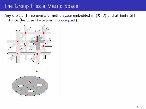
The Group Γ as a Metric Space

Any orbit of Γ represents a metric space embedded in (X , d) and at finite GHdistance (because the action is cocompact).

Two possible metrics in Γ:

Orbit metric: fix x0 ∈ Γ and definedΓ,x0 (γ1, γ2) := d(γ1(x0), γ2(x0))

Word metric: Let S = s1, . . . , sk be asymmetric set of generators of Γ. For eachγ ∈ Γ we denote

‖γ‖S := minn ∈ N : γ ∈ Sn

and we define dS(γ1, γ2) := ‖γ−11 γ2‖S .

These metrics are both left-invariant and theyare all bi-Lipschitz equivalent.

Idea: We study the asymptotic cone of Γ as a metric space.

21 / 34

Idea: We study the asymptotic cone of Γ as a metric space.21 / 34

Asymptotic Cone of a Group

Let Γ be a finitely generated group with a metric dΓ (one of the metric introducedbefore).

Γ abelian: Γ ' Zk ⊕ Γ0, where k = rank Γ and Γ0 is the torsion subgroup (afinite group). Then, the asymptotic cone is G∞ ' Rk and the asymptoticdistance is related to the stable norm, i.e., the unique norm ‖ · ‖∞ such thatfor each γ ∈ Zk :

‖γ‖∞ = limn→+∞

dΓ(0, nγ)

If Γ has polynomial growth, i.e., there exist C > 0 and K > 0 such that

]γ ∈ Γ : ‖γ‖S ≤ r ≤ CrK ∀ r > 0

then the asymptotic cone exists and it is unique (Gromov, 1981).

Gromov proved that Γ has polynomial growth if and only if it is virtuallynilpotent, i.e., it contains a nilpotent subgroup of finite index.

Polynomial growth is the optimal condition to ensure both existence anduniqueness of the asymptotic cone.

22 / 34

‖γ‖∞ = limn→+∞

dΓ(0, nγ)

]γ ∈ Γ : ‖γ‖S ≤ r ≤ CrK ∀ r > 0

22 / 34

‖γ‖∞ = limn→+∞

dΓ(0, nγ)

]γ ∈ Γ : ‖γ‖S ≤ r ≤ CrK ∀ r > 0

22 / 34

‖γ‖∞ = limn→+∞

dΓ(0, nγ)

]γ ∈ Γ : ‖γ‖S ≤ r ≤ CrK ∀ r > 0

22 / 34

Nilpotent Groups

A finitely generated group Γ is said to be nilpotent if the lower central series endsafter finitely many steps:

Γ(1) := Γ ≥ Γ(2) := [Γ(1), Γ] ≥ . . . ≥ Γ(i+1) := [Γ(i), Γ] ≥ . . . ≥ Γ(r) > Γ(r+1) = e,

where [·, ·] denotes the commutator subgroup and r is called the nilpotency classof Γ.

Examples:

Abelian groups (r = 1);

Quaternionic group Q8 (r = 2) ← (smallest non-abelian example)

Heisenberg group H2n+1(Z) (r = 2):

H2n+1(Z) = 〈a1, b1, . . . , an, bn, t : [ai , bi ] = t ∀ i = 1, . . . , n and all others brackets = 0〉.

Nilpotent groups have polynomial growth (Wolf, 1968). In particular, Bass (1972)proved that the rate is

K =r∑

k · rank(

Γ(k)/Γ(k+1)),

also called the homogeneous dimension of Γ.

23 / 34

Nilpotent Groups

Examples:

K =r∑

k · rank(

Γ(k)/Γ(k+1)),

also called the homogeneous dimension of Γ.

23 / 34

Nilpotent Groups

Examples:

K =r∑

k · rank(

Γ(k)/Γ(k+1)),

also called the homogeneous dimension of Γ.23 / 34

Asymptotic Cone of a Nilpotent Group

In order to study the asymptotic cone of a nilpotent group, it would be useful toembed it into some ambient space (similarly to what happens with Zn and Rn).

Theorem [Malcev, 1951]

Let Γ be a f.g. torsion free nilpotent group. There exists a unique (up toisomorphisms) simply connected, nilpotent Lie group G , in which Γ can beembedded as a cocompact discrete subgroup (G is the Malcev closure of Γ).

Idea of the proof:

Γ has a canonical set of generators, namely there exist γ1, . . . , γd such thatevery γ ∈ Γ can be written uniquely as γ = γα1

1 · . . . · γαd

d , for αi ∈ Z.

The group structure on Γ can be then described in terms of polynomialrelations in the αi ’s −→ new group structure on Zd .

These polynomial relations can be used to define a group structure on Rd ,which will provide the Malcev closure G .

Remark: d = dimG =∑r

k=1 rank(Γ(k)/Γ(k+1)

24 / 34

Idea of the proof:

1 · . . . · γαd

d , for αi ∈ Z.

24 / 34

Idea of the proof:

1 · . . . · γαd

d , for αi ∈ Z.

24 / 34

Idea of the proof:

1 · . . . · γαd

d , for αi ∈ Z.

24 / 34

Idea of the proof:

1 · . . . · γαd

d , for αi ∈ Z.

24 / 34

Idea of the proof:

1 · . . . · γαd

d , for αi ∈ Z.

24 / 34

Stratified Lie Algebra and Dilations

A Lie Algebra g is called a stratified algebra if it admits a stratification, i.e., thereexist vector subspaces V1, . . . ,Vr ⊂ g (called strata) such that

g = V1 ⊕ . . .⊕ Vr

and [Vj ,V1] = Vj+1 for j = 1, . . . , r , with Vr 6= 0 and [Vr ,V1] = 0([V ,W ] denotes the subspace generated by commutators).

A graded Lie group G is a simply connected Lie group whose algebra is stratified.

A stratified algebra is nilpotent (some sort of vice-versa is true).

The first stratum V1 completely determines the other strata and it is inbijection with the abelianization g

[g,g] .

We can define dilations: for each λ ∈ R we define δλ : g −→ g which is analgebra automorphism defined linearly by imposing δλ(v) = λiv for everyv ∈ Vi , with i = 1, . . . , r . Using the exponential map, we can define theassociated group automorphisms δλ : G −→ G .

25 / 34

g = V1 ⊕ . . .⊕ Vr

[g,g] .

25 / 34

g = V1 ⊕ . . .⊕ Vr

[g,g] .

25 / 34

g = V1 ⊕ . . .⊕ Vr

[g,g] .

25 / 34

g = V1 ⊕ . . .⊕ Vr

[g,g] .

25 / 34

If Γ is a finitely generated nilpotent group, not only the asymptotic cone(G∞, d∞) exists and is unique, but it also enjoys many interesting properties(Pansu, 1983) −→ G∞ it is related to the Malcev closure of Γ.

G∞ is a simply connected, nilpotent Lie group (with nilpotency class r).

dimG∞ =∑r

Γ embeds in G∞ as a cocompact lattice.

Its Lie algebra g∞ is stratified: g∞ = V1 ⊕ . . .⊕ Vr . Therefore, it hasdilations δλ : g∞ −→ g∞ for each λ > 0 (or, via the exp. map,δλ : G∞ −→ G∞).

d∞ is a Carnot-Caratheodory distance and d∞(δλ(x), δλ(y)) = λd∞(x , y)for all x , y ∈ G∞ and λ > 0.

Let ∆ ⊂ TG∞ the horizontal distribution induced by V1. There exists anorm ‖ · ‖∞ on ∆ (obtained similarly to what done for the stable norm)and d∞ is the sub-Riemannian distance induced by (G∞,∆, ‖ · ‖∞),i.e., for x , y ∈ G∞ we define:

d∞(x , y) = inf∫ T

0‖γ(t)‖∞ : γ : [0,T ]→ G∞is horizontal and︸︷︷︸

γ(t)∈∆ for a.e. t∈[0,T ]

γ(0) = x , γ(T ) = y

26 / 34

dimG∞ =∑r

d∞(x , y) = inf∫ T

γ(t)∈∆ for a.e. t∈[0,T ]

γ(0) = x , γ(T ) = y

26 / 34

dimG∞ =∑r

d∞(x , y) = inf∫ T

γ(t)∈∆ for a.e. t∈[0,T ]

γ(0) = x , γ(T ) = y

26 / 34

dimG∞ =∑r

d∞(x , y) = inf∫ T

γ(t)∈∆ for a.e. t∈[0,T ]

γ(0) = x , γ(T ) = y

26 / 34

dimG∞ =∑r

d∞(x , y) = inf∫ T

γ(t)∈∆ for a.e. t∈[0,T ]

γ(0) = x , γ(T ) = y

26 / 34

dimG∞ =∑r

d∞(x , y) = inf∫ T

γ(t)∈∆ for a.e. t∈[0,T ]

γ(0) = x , γ(T ) = y

26 / 34

Main Theorem (Part 1/3)

Let H : T ∗X −→ R be a Γ-invariant Tonelli Hamiltonian and let L : TX −→ R be theassociated Γ-invariant Tonelli Lagrangian.

For ε > 0, let Xε denote the rescaled metric spaces (X , dε := εd) and consider therescaled Hamilton-Jacobi equation:

(HJε)

ε(x , t) + H(x , 1ε∂xu

ε(x , t)) = 0 x ∈ Xε, t > 0uε(x , 0) = fε(x),

where fε : Xε −→ R are equiLipschitz with respect to the metrics dε and, as ε goes tozero, they converge uniformly on compact sets to a function f : G∞ −→ R with at mostlinear growth.

1. The rescaled solutions (for x ∈ Xε and T > 0)

uε(x ,T ) = inf

fε(γ(0)) +

0L(γ(t), εγ(t)) dt

∣∣ γ ∈ C1([0,T ],Xε), γ(T ) = x

converge uniformly on compact sets of G∞ × (0,+∞) to a functionu : G∞ × (0,+∞)→ R.

27 / 34

Let H : T ∗X −→ R be a Γ-invariant Tonelli Hamiltonian and let L : TX −→ R be theassociated Γ-invariant Tonelli Lagrangian.

For ε > 0, let Xε denote the rescaled metric spaces (X , dε := εd) and consider therescaled Hamilton-Jacobi equation:

(HJε)

ε(x , t) + H(x , 1ε∂xu

ε(x , t)) = 0 x ∈ Xε, t > 0uε(x , 0) = fε(x),

where fε : Xε −→ R are equiLipschitz with respect to the metrics dε and, as ε goes tozero, they converge uniformly on compact sets to a function f : G∞ −→ R with at mostlinear growth.

1. The rescaled solutions (for x ∈ Xε and T > 0)

uε(x ,T ) = inf

fε(γ(0)) +

∣∣ γ ∈ C1([0,T ],Xε), γ(T ) = x

converge uniformly on compact sets of G∞ × (0,+∞) to a functionu : G∞ × (0,+∞)→ R.

27 / 34

2. For x ∈ G∞ and T > 0:

u(x ,T ) = infy∈G∞

f (y) + TL

(δ1/T (y−1x)

where L : G∞ −→ R depends only on the Hamiltonian H, it is superlinear, i.e.,

∀ A > 0 ∃ B = B(A) ≥ 0 : L(x) ≥ A d∞(e, x)− B ∀ x ∈ G∞

and convex, namely

L(δλ(x) · δ1−λ(y)

)≤ λL(x) + (1− λ)L(y) ∀ λ ∈ (0, 1) and ∀ x , y ∈ G∞.

We shall call this function Generalized Mather’s β-function.

3. For each x ∈ G∞

L(x) := infσ∈Hx

β(π(σ(s))) ds,

where Hx denotes the set of absolutely continuous horizontal curvesσ : [0, 1] −→ G∞ connecting e to x , β : H1(X/Γ;R) −→ R is Mather’s β-functionassociated to the Lagrangian L projected on T (X/Γ), andπ : g∞ −→ g∞

[g∞,g∞]−→ H1(X/Γ;R).

28 / 34

2. For x ∈ G∞ and T > 0:

f (y) + TL

(δ1/T (y−1x)

where L : G∞ −→ R depends only on the Hamiltonian H, it is superlinear, i.e.,

∀ A > 0 ∃ B = B(A) ≥ 0 : L(x) ≥ A d∞(e, x)− B ∀ x ∈ G∞

and convex, namely

L(δλ(x) · δ1−λ(y)

)≤ λL(x) + (1− λ)L(y) ∀ λ ∈ (0, 1) and ∀ x , y ∈ G∞.

We shall call this function Generalized Mather’s β-function.

3. For each x ∈ G∞

L(x) := infσ∈Hx

β(π(σ(s))) ds,

where Hx denotes the set of absolutely continuous horizontal curvesσ : [0, 1] −→ G∞ connecting e to x , β : H1(X/Γ;R) −→ R is Mather’s β-functionassociated to the Lagrangian L projected on T (X/Γ), andπ : g∞ −→ g∞

[g∞,g∞]−→ H1(X/Γ;R).

28 / 34

u is the unique viscosity solution to the following problem:∂t u(x , t) + H(∇Hu(x , t)) = 0 (x , t) ∈ G∞ × (0,∞)u(x , 0) = f (x) x ∈ G∞,

where ∇Hu(x , t) denotes the horizontal gradient of u(·, t) (with respect to the

x-component) and H :(

g∞[g∞,g∞]

)∗−→ R is the convex conjugate of β restricted

to the subspace π(g∞) ⊆ H1(X/Γ;R).

29 / 34

Some Ideas on the Proof: Rescaling Maps

Note: For simplifying the presentation, let us assume that G∞ coincides with theMalcev closure of Γ.

Fix x0 ∈ X and choose a fundamental domain Ω of the action of Γ in G∞, suchthat x0 ∈ Ω.

Rescaling maps: For each ε > 0 we define a map hε : G∞ −→ Γ in thefollowing way. If x ∈ G∞, then hε(x) = γ such that δ 1

ε(x) ∈ γ · Ω.

Properties:

1. For each R > 0, there exists θ(ε)→ 0 as ε→ 0+, such that hε mapsthe ball Bd∞

R (e) into BdεR+θ(ε)(x0).

2. δε(hε(x)) −→ x in G∞ and if x 6= y then δε(hε(x)hε(y)−1) −→ x y−1

in G∞.

30 / 34

ε(x) ∈ γ · Ω.

Properties:

in G∞.

30 / 34

ε(x) ∈ γ · Ω.

Properties:

in G∞.

30 / 34

ε(x) ∈ γ · Ω.

Properties:

in G∞.

30 / 34

Some Ideas on the Proof: Notion of Convergence

Convergence: Let Fε : Xε → R and F : G∞ → R. We say that:

1. Fε → F poinwise as ε→ 0+, if for each x ∈ G∞ we have

limε→0+

Fε(hε(x) · x0) = F (x).

2. Fε → F locally uniformly as ε→ 0+, if for each R > 0 we have

limε→0+

supBd∞R (e)

∣∣Fε(hε(x) · x0)− F (x)∣∣ = 0.

Note: If Fε are equicontinuous, also this notion is independent of x0.

31 / 34

Some Ideas on the Proof: Notion of Convergence

Convergence: Let Fε : Xε → R and F : G∞ → R. We say that:

1. Fε → F poinwise as ε→ 0+, if for each x ∈ G∞ we have

limε→0+

Fε(hε(x) · x0) = F (x).

2. Fε → F locally uniformly as ε→ 0+, if for each R > 0 we have

limε→0+

supBd∞R (e)

∣∣Fε(hε(x) · x0)− F (x)∣∣ = 0.

Note: If Fε are equicontinuous, also this notion is independent of x0.

31 / 34

Some Ideas on the Proof: Rescaled Mane potential

Recall the representation formula for the solution to (HJε):

uε(x ,T ) = inffε(γ(0)) +

∣∣ γ ∈ C1([0,T ],Xε), γ(T ) = x

We define the Mane potential associated to Lε(x , v) = L(x , εv) as (let x , y ∈ Xand T > 0):

Φε(x , y ,T ) := inf

∣∣ γ ∈ C1([0,T ],Xε), γ(0) = x , γ(T ) = y

∫ T/ε

0L(γ(t), γ(t)) dt

∣∣ γ ∈ C1([0,T/ε],X ), γ(0) = x , γ(T/ε) = y

Note: We are assuming that the Mane critical value of L : T (X/Γ)→ R is zero.

32 / 34

0L(γ(t), εγ(t)) dt︸︷︷︸

Mane potential

∣∣ γ ∈ C1([0,T ],Xε), γ(T ) = x

∣∣ γ ∈ C1([0,T ],Xε), γ(0) = x , γ(T ) = y

∫ T/ε

0L(γ(t), γ(t)) dt

∣∣ γ ∈ C1([0,T/ε],X ), γ(0) = x , γ(T/ε) = y

32 / 34

0L(γ(t), εγ(t)) dt︸︷︷︸

Mane potential

∣∣ γ ∈ C1([0,T ],Xε), γ(T ) = x

∣∣ γ ∈ C1([0,T ],Xε), γ(0) = x , γ(T ) = y

∫ T/ε

0L(γ(t), γ(t)) dt

∣∣ γ ∈ C1([0,T/ε],X ), γ(0) = x , γ(T/ε) = y

32 / 34

Some Ideas on the Proof: Limit of Rescaled Mane potential

Let us define the following function

Fε : G∞ × (0,+∞) −→ R(x ,T ) 7−→ Φε(x0, hε(x) · x0,T ).

Rescaling property: Fε(x ,S) = ST F T

S ε(δ T

S(x),T ) for all x ∈ G∞ and S ,T > 0.

Proposition

For all x ∈ G∞ and T > 0

∃ limε→0+

Fε(x ,T ) =: β(x ,T ).

Clearly, β(x ,S) = ST β(δ T

The effective Lagrangian is defined as L(x) := β(x , 1). It has an explicitexpression in terms of Mather’s β function (see statement of the theorem).

33 / 34

Fε : G∞ × (0,+∞) −→ R(x ,T ) 7−→ Φε(x0, hε(x) · x0,T ).

S ε(δ T

Proposition

∃ limε→0+

Fε(x ,T ) =: β(x ,T ).

33 / 34

Fε : G∞ × (0,+∞) −→ R(x ,T ) 7−→ Φε(x0, hε(x) · x0,T ).

S ε(δ T

Proposition

∃ limε→0+

Fε(x ,T ) =: β(x ,T ).

33 / 34

Fε : G∞ × (0,+∞) −→ R(x ,T ) 7−→ Φε(x0, hε(x) · x0,T ).

S ε(δ T

Proposition

∃ limε→0+

Fε(x ,T ) =: β(x ,T ).

33 / 34

Some Ideas on the Proof: Convergence

Then one can show that uε→ u locally uniformaly in G∞ × (0,+∞) as ε goes tozero, where

f (y) + TL

(δ1/T (y−1x)

Moreover, from this Hopf-like representation formula & a result by Balogh,Calogero and Pini (2014), we can deduce that u solves a Hamilton-Jacobiequation associated to some specific effective Hamiltonian H (see the statementof the theorem):

∂t u(x , t) + H(∇Hu(x , t)) = 0 (x , t) ∈ G∞ × (0,∞)u(x , 0) = f (x) x ∈ G∞,

34 / 34

Thank you for your attention!

on the homogenization of the hamilton-jacobi...

Documents