geospatial intermodal freight transport (gift) model with
TRANSCRIPT
Evaluating the Environmental Attributes of Freight Traffic along the U.S West Coast
Geospatial Intermodal Freight Transport (GIFT) Model with Cargo Flow Analysis
Prepared for the California Air Resources Board California Environmental Protection Agency
Contract No.: 07-314
James J. Corbett, University of Delaware
J. Scott Hawker, Rochester Institute of Technology James J. Winebrake, Rochester Institute of Technology
Presented at the ARB Air Pollution Seminar Series
7 June 2011
1

Project Objective • Quantify environmental impact of containerized freight movement in the
West Coast Freight Gateway and Corridor
• Apply a GIS-based model modified to include California-specific inputs
• Demonstrate potential system improvements to achieve GHG reductions and address environmental issues related to freight transport
Source: U.S. Maritime Administration
2

Discussion Items
• Background on Freight Transport
• Reasons to Model Alternatives
• GIFT Model
• Research Methodology
• Results and Analysis
• Summary
3

FREIGHT TRANSPORT BACKGROUND
Attributes of Freight Transport
© http://www.freightcaptain.com/
4
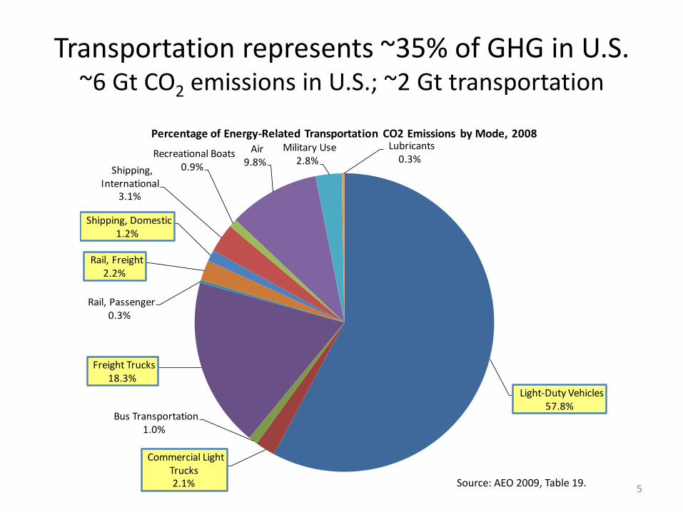
Light-Duty Vehicles57.8%
Commercial Light Trucks2.1%
Bus Transportation1.0%
Freight Trucks18.3%
Rail, Passenger0.3%
Rail, Freight2.2%
Shipping, Domestic1.2%
Shipping, International
3.1%
Recreational Boats0.9%
Air9.8%
Military Use2.8%
Lubricants0.3%
Percentage of Energy-Related Transportation CO2 Emissions by Mode, 2008
Source: AEO 2009, Table 19.
Transportation represents ~35% of GHG in U.S. ~6 Gt CO2 emissions in U.S.; ~2 Gt transportation
5
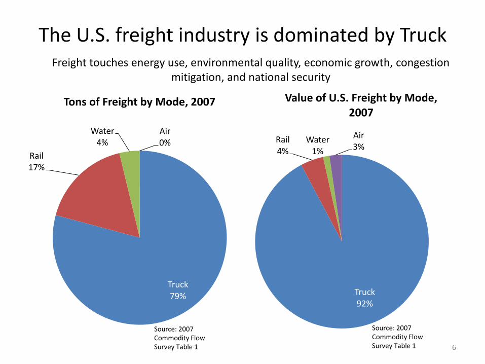
The U.S. freight industry is dominated by Truck
Truck 79%
Rail 17%
Water 4%
Air 0%
Tons of Freight by Mode, 2007
Source: 2007 Commodity Flow Survey Table 1
Truck 92%
Rail 4%
Water 1%
Air 3%
Value of U.S. Freight by Mode, 2007
Source: 2007 Commodity Flow Survey Table 1
Freight touches energy use, environmental quality, economic growth, congestion mitigation, and national security
6

Freight Overview • Energy use within freight mode is proportional to work done
• Carbon intensity (and other emissions) not symmetric across modes
Global and US Cargo Flows (Gt-km) by Mode (2005)
James J. Corbett, James J. Winebrake ©2010
1
10
100
1,000
10,000
100,000
Road Shipping Aviation Rail
Ca
rgo
Vo
lum
e (
Gtk
m)
U.S. Freight (Gtkm) EU25 Freight World Freight Gtkm
1
10
100
1,000
10,000
Truck Rail Ship (Domestic) Air
Gtk
m/y
r an
d T
gCO
2/y
r
Annual Freight Demand and CO2 Emissions by Mode, 2005
Gtkm/yr TgCO2/yr
7

Goods Movement and GDP
3000
3200
3400
3600
3800
4000
4200
4400
4600
4800
6000 7000 8000 9000 10000 11000 12000
Ton
-Mile
s (B
illio
ns)
GDP (Billions, 2000$)
Ton-Miles v. GDP for the U.S. (1987-2005)
For every trillion dollar increase in GDP, we expect an additional 242 billion ton-miles.
Source: Corbett and Winebrake, 2008. James J. Corbett, James J. Winebrake ©2010
8

Calculating Impacts from the Bottom Up
Calculators developed by RIT and the University of Delaware to support research activities under the Sustainable Intermodal Freight Transportation Research (SIFTR) program
MODAL MODELING OF POSSIBILITIES
9

THE GIFT MODEL Geospatial Intermodal Freight Transportation Model
10

VISUALIZING GOALS MODELING
ALTERNATIVES
Intermodal freight network optimization model to evaluate objective tradeoffs.
Developing resources for “table-top” exercises with industry and agencies.
Evaluates performance against benchmarks and optimizes with respect to possible targets
Web-version in development.
Geospatial Intermodal Freight Transportation (GIFT) Model
Decision makers can explore tradeoffs among alternative
routes, across modes, and identify optimal routes for
economic, energy and environmental objectives.
11

How are we using GIFT?
• Table-top exercises with leaders in transportation – Modal experts and industry decision makers
– Public infrastructure planners at regional and national levels
– Environmental, energy interests in public and private sectors
infrastructure fuels technologies operations logistics demand
12

The GIFT Model Integrating the National Transportation Atlas Database (NTAD) Components
NTAD Road Network NTAD Rail Network
STEEM Water Network
Intermodal Freight Transport
Each segment and spoke of the network contains temporal, economic, and environmental attributes- called “cost factors”
Attribute values used to search for routes that minimize the total “Costs”
13

The Geospatial Intermodal Freight Transportation (GIFT) Model
• GIS-based optimization model
• Intermodal network (Road, Rail, Water and Facilities)
• Calculation of least time, least cost , least energy and least emissions (CO2, PM10, NOx, SOx, VOC) routes
• Tool to aid decision makers understand environmental, economic, energy impact of intermodal freight transportation and to compare trade-offs among various policy scenarios
14
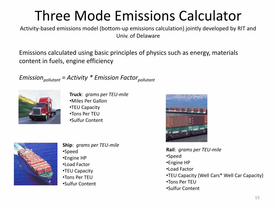
Three Mode Emissions Calculator
Activity-based emissions model (bottom-up emissions calculation) jointly developed by RIT and Univ. of Delaware
Truck: grams per TEU-mile •Miles Per Gallon •TEU Capacity •Tons Per TEU •Sulfur Content
Rail: grams per TEU-mile •Speed •Engine HP •Load Factor •TEU Capacity (Well Cars* Well Car Capacity) •Tons Per TEU •Sulfur Content
Ship: grams per TEU-mile •Speed •Engine HP •Load Factor •TEU Capacity •Tons Per TEU •Sulfur Content
Emissions calculated using basic principles of physics such as energy, materials content in fuels, engine efficiency Emissionpollutant = Activity * Emission Factorpollutant
15

RESEARCH METHODOLOGY
California-specific application of GIFT Preparing, importing and processing data in ArcGIS
16

Structure and use of the GIFT model
Vehicle and Facility Emissions and Operations Data• Trucks, Trains, Ships• Ports, Rail yards,
Distribution centers
Transportation Network Geospatial Data• Highways, Railroads,
Waterways• Multimodal transfer
facilities
Freight Flow Data• Originations/
Destinations• Volumes
Freight Transportation Data
Vehicle and FacilitySelection and Characterization
Scenario Configuration
Data
Network Configuration• Select cost
attributes to compare
• Select cost attributes to minimize
Freight Flow Selection and Characterization
Geospatial Intermodal Freight
Transportation (GIFT) Analysis
Scenario Data Comparison and Analysis for Case
Studies
Scenario Analysis Results
Find Least “Cost” Routes
Source:(J.S. Hawker, et al., 2010)
17

Methodology Gathering Data
• Commodity Flow Survey 2007 – National freight flow figures which include estimated shipping volumes (value,
tons, and ton-miles) by commodity and mode of transportation at varying levels of geographic detail
– Lists freight tonnage between the major O-D pairs
• Port Generated Traffic- US Army Corps of Engineers 2007 – Waterborne container traffic for US Port/ Waterway 2007
• Cambridge Systematics Origin-Destination (O-D) Database – Disaggregated Freight Analysis Framework 2.2 (FAF 2) data at a county level
– FAF2 data publicly available and built from CFS and other data sources
18

Route Identification Method Building a multiple O-D framework
19
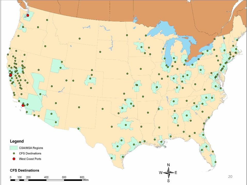
20

Plural methods for allocating freight flows Approaches to distributing freight using CFS data
Outside CA, freight split evenly between destinations in the “Remainder of” regions in the states
21

Methodology Emissions Assumptions
Mode Type/Spoke Type
CO2 Emissions by Mode Type (g/TEU-Mile)
Intermodal Transfer CO2 Emissions by Spoke Type (g/TEU)
Mode Attributes
Truck MY 1998-02
830 9200 •Fuel Economy: 6 MPG •TEU Capacity: 2 •Tons Per TEU: 10 •Engine Efficiency: 42% •Fuel Type: Distillate Diesel with 15ppm Sulfur
Rail Tier 1 Line Haul
320 4100 •Speed: 25 mph •Engine HP: 8000 •Load Factor: 70% •Engine Efficiency: 42% •TEU Capacity: 400 •Tons Per TEU: 10 •Fuel Type: Distillate Diesel with 15ppm Sulfur
Ship ‘Dutch Runner ‘
410 2500 •Speed: 13.5 mph •Engine HP: 3070 •Load Factor: 80% •Engine Efficiency: 40% •TEU Capacity: 220 •Tons Per TEU: 10 •Fuel Type: Marine Diesel with 5000 ppm Sulfur 22
RESULTS AND ANALYSES Analyzing the benefits of a Modal Shift in Freight
23

Least-Time Freight Flow Results
From Ports To Ports
24

Least-CO2 Scenario Results
From Ports To Ports
25

Air Basin Allocation Example
Least Time Least CO2
26

Air Basin Emissions Allocation Change (difference between “least-time” and “least CO2” routing in GIFT)
27
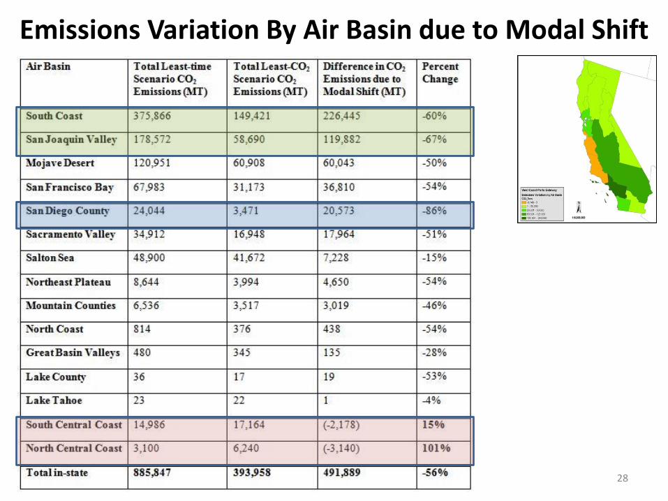
Emissions Variation By Air Basin due to Modal Shift
28

Comparison of Emissions Across Scenarios Least Time Scenario
Least CO2 Scenario
Total Emissions Comparison
29

SUMMARY
30

Conclusion
• Idealized use of least-CO2 routing constraints illustrates emissions savings can be achieved through modal shifts.
• Total emissions reductions of 1.7 MMT (~0.5 MMT within California)of CO2 achievable through a nationwide modal shift of West-Coast ports generated goods movement.
• Results are based on assumption that all port-related goods movement occurs through truck (not adjusted for amount moving through rail and other modes)
• Results have relevance for consideration of system-wide improvements that may achieve energy savings, CO2 reductions, and associated benefits for air quality.
31
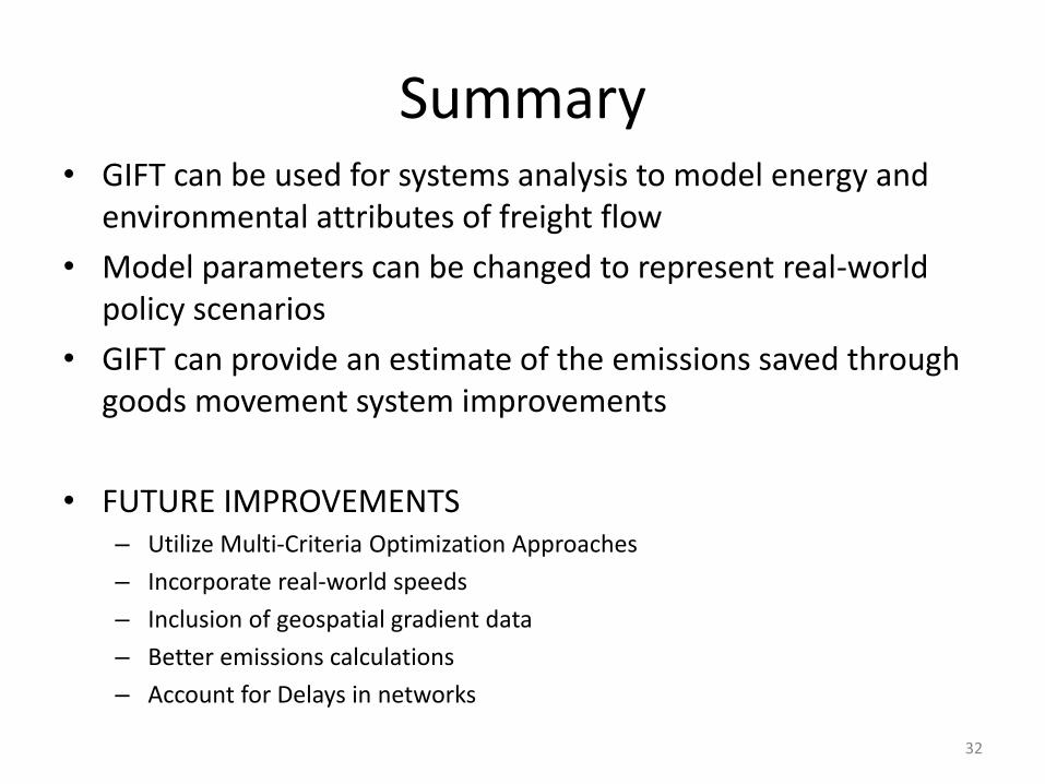
Summary • GIFT can be used for systems analysis to model energy and
environmental attributes of freight flow
• Model parameters can be changed to represent real-world policy scenarios
• GIFT can provide an estimate of the emissions saved through goods movement system improvements
• FUTURE IMPROVEMENTS – Utilize Multi-Criteria Optimization Approaches
– Incorporate real-world speeds
– Inclusion of geospatial gradient data
– Better emissions calculations
– Account for Delays in networks
32

Questions?
33