fish&rivers in stress - ch.9,10, acknowls.pdf
TRANSCRIPT

Environmental factors associated with carp populations 225
CRC For Freshwater Ecology RACAC NSW Fisheries
9 The role of the natural environment andhuman impacts in determining biomassdensities of common carp in New SouthWales rivers
P.D. DriverA, J.H. HarrisB, R.H. NorrisA, and G.P. ClossC
A Cooperative Research Centre for Freshwater Ecology, University of Canberra, PO Box 1, Belconnen, ACT, 2616
B Cooperative Research Centre for Freshwater Ecology, NSW Fisheries Research Institute, PO Box 21, Cronulla, NSW,
2230.C
Department of Zoology, University of Otago, PO Box 56, Dunedin, New Zealand.
Summary
The environmental factors associated with the biomass density (kg site-1) of common carp (Cyprinuscarpio L.) in rivers of New South Wales were explored. Carp were not found in any of the 20 montane sites. Ininland rivers, carp were present in all sites below an altitude of ca. 500 m ASL. In coastal river systems, thedistribution of carp was restricted to only six sites in an altitudinal range of 0-60 m ASL within regulatedlowland rivers. All inland rivers had higher carp biomass densities than the coastal rivers. Carp biomass densitiesin the inland rivers were found to increase slightly (r2 = 0.18) with altitude, for altitudes up 500 m ASL. Theseslightly higher carp biomass densities in the inland rivers were associated with an abundance of riffle habitat andcoarse particles in the substratum. This unexpected association was probably the result of upstream migration ofadult carp from spawning habitats, and the presence of barriers to fish dispersal including dams and natural riverfeatures. The likely spawning habitats from which adult carp migrated were lowland areas (below 200 m ASL)and water storages in mid-altitudes (200-500 m ASL).
Across New South Wales, higher carp biomass densities were associated with variables indicating humanimpacts, in particular the effects of dams and agriculture. Alteration of flows and water temperatures, physicalbarriers to fish migration, carp spawning habitat created in artificial lakes, and agricultural effects on waterquality are all factors suggested as leading to higher carp biomass densities.
These results suggest that river management focused on carp spawning habitat, migration from thesespawning areas, and the effects of agriculture and river regulation would be effective in reducing carp biomassdensities, improving water quality and increasing native fish stocks.

226
CRC For Freshwater Ecology RACAC
INTRODUCTION
Justifications for this study
Most studies of common carp (Cyprinus carpio hereafter referred to as carp) and their
habitat have considered only the impacts of carp at smaller scales, such as in billabongs or
experimental ponds (e.g. papers cited within Taylor et al. 1984 and King 1995). These studies
provide important information regarding the local effects of carp on water chemistry and
freshwater biota, and demonstrate that the impacts of carp are partly dependent on the biomass
density (kg ha–1) of carp. However, additional information is required for quantifying and
controlling the effects of carp in Australia. Small-scale effects of carp (e.g. increased turbidity)
can be obscured by processes occurring at larger spatial scales (e.g. flow regulation or geology)
(Hume et al. 1983; Wiens 1989). Furthermore, how the environment affects carp distribution and
abundance, and ultimately the impact carp can have, has been poorly considered. To partly fill
these knowledge gaps, this study describes the distribution and the kilogram-per-site biomass
density of carp (carp biomass density) in relation to the physical environment associated with
rivers at the catchment scale.
Carp in Australia
Carp in Australia are an alien benthic omnivorous fish species derived from the wild carp
of Asia Minor and around the Caspian Sea (Balon 1974). They are widespread in southeastern
Australia and can constitute most of the total fish biomass (e.g. in the Murray River, Gehrke et al.
1995). There are four strains of carp in Australia. The two strains of most concern to fisheries
managers are the Boolara or River carp and the Koi carp (Shearer and Mulley 1978; Harris 1995;
Davis 1997). Although the Boolara strain is the most abundant and widespread, the Koi strain is
more abundant in some areas such as in Lake Burley Griffin (Australian Capital Territory), Lake
Crescent (Tasmania), and the Shoalhaven and Richmond Rivers (New South Wales) (Shearer and
Mulley 1978; Harris 1995; Davis 1997). The Prospect strain of carp has a distribution limited to
Prospect Reservoir, and the Yanco strain is limited in distribution and has been genetically diluted
by the Boolara strain (Shearer and Mulley 1978; Davis 1997). The four strains are not
differentiated in this survey.
Environmental factors associated with carp
Although carp have been found in a wide range of habitats, optimal habitat for carp in
Australia and overseas is generally considered to be low-altitude, slow-flowing waters, with access

Environmental factors associated with carp populations 227
NSW Fisheries - Office of Conservation
to shallow, vegetated habitat for spawning, as would be found in larger rivers or billabongs (e.g.
McCrimmon 1968; Panek 1987; Rahel and Hubert 1991; Brown and Coon 1994; Brown 1996;
Lyons 1996; McDowall 1996). Carp have often been found in waters that are turbid, with poor
water-quality (e.g. McCrimmon 1968; Panek 1987; McDowall 1996). In addition, due to benthic
feeding adaptations (Sibbing et al. 1986) adult carp may also be more reliant on substrata with
fine aggraded particles, such as silt.
High biomass densities (kg ha-1) of carp have been associated with the loss of native fish
species, reduction in aquatic macrophyte abundance and deterioration of water quality; in
particular an increase in turbidity (Crivelli 1983; Taylor et al. 1984; Fletcher et al. 1985;
Breukelaar et al. 1994; Faragher and Harris 1994; Gehrke and Harris 1994; Harris 1995; King
1995; Roberts et al. 1995; Robertson et al. 1995). The association between carp biomass densities
and measures of turbidity and aquatic vegetation abundance would be less significant when
measured at catchment scales because larger-scale physical and ecological processes tend to
obscure small-scale effects (Wiens 1989). This was demonstrated in a study within the Goulburn
River catchment of north-eastern Victoria where background levels of turbidity and flow variation
obscured the effects of carp on turbidity and macrophytes (Fletcher et al. 1985).
Some of the strongest associations likely to occur at the catchment scale are between carp
and human impacts. The broad ecological tolerances of carp suggest that carp populations would
thrive relative to native fish populations under human disturbance (McCrimmon 1968; Crivelli
1981; Panek 1987; Arthington et al. 1989; Harris 1997). Studies overseas have found that carp
can become a much larger component of fish communities after disturbances in flow, damming
and alteration of the stream bed (e.g. Whitley 1974 and Sparks and Starret 1975, both cited in
Welcomme 1979; Hoyt and Robison 1980; Winston et al. 1991). Large dams may be an
important component of these effects leading to increase in carp abundance. Large dams in the
United States of America have had upstream and downstream effects that lead to major changes in
the fish community, and an increase in carp numbers (e.g. Hoyt and Robison 1980; Winston et al.
1991). These local fish community changes due to regulation may reflect larger-scale changes
favouring carp. Such large-scale effects were indicated by an Australian study (Gehrke et al.
1995) which found that a measure of river regulation (measuring the deviation from natural
flows) was positively associated with carp-dominated fish communities. Other effects of human
activities within river catchments have been associated with similar changes in fish communities.
Agricultural activities have been associated with substantial reductions in flows due to irrigation,
chemical enrichment, aggradation of fine sediments and changes in stream morphology
(Cadwallader 1978; Rinne 1990; Koehn and O’Connor 1990; Faragher and Harris 1994;
Metzeling et al. 1995; Brierley et al. 1996; Finlayson and Silburn 1996). In Australia, with these
types of human impact there has been a corresponding and severe decline in native fish
communities (e.g. Cadwallader 1978; Pierce 1988; Arthington et al. 1989; Faragher and Harris
1994; Cullen et al. 1996). Under these circumstances, carp would also be expected to prosper.
228
CRC For Freshwater Ecology RACAC
Objectives
This study of carp in New South Wales rivers first describes the differences in carp biomass
density across the spatial and temporal scales covered by the NSW Rivers Survey. This determined
the spatial scales that were comparable in terms of carp biomass density (e.g. all inland rivers).
To test our predictions regarding environmental conditions and carp, the presence of carp
and carp biomass density were related to large-spatial-scale variables (e.g. minimum annual
temperatures, catchment area, livestock densities), smaller-spatial-scale habitat description (e.g.
conductivity, depth, substrate type) and long-term climatic data. More specifically, we tested
whether the following environmental conditions were associated with carp and high carp biomass
densities:
1. Low altitude
2. Low velocity flows
3. Large dams
4. High agricultural land use
METHODS
Field collection of data
The statistical design and sampling regime used in the NSW Rivers Survey are described in
detail in Chapter 1. However, details especially relevant to this chapter are repeated here. A suite of
fish-sampling techniques standardised for major habitat types were used at every site to ensure
accurate representation of fish species present. The number of fish of each species was recorded
for each site. For each replicate unit of gear used for fish sampling only the first ten fish of any
species had their length measured. Habitat characteristics were assessed using estimates that
involved a rapid, subjective grading system for features such as flow, depth, width, substrate,
vegetation and observer-assessed turbidity (Table 9.1, Table 9.2). Dissolved oxygen, pH,
conductivity and temperature were also measured, using a Horiba U-10 water quality meter. The
region, river type, season, year, date and times of the use of each gear type were also recorded
(Table 9.2).

Environmental factors associated with carp populations 229
NSW Fisheries - Office of Conservation
Preparation of data for analysis
Conversion of data for analyses
Habitat variables using the rapid, subjective grading system were converted to numerical
data as shown in Table 9.1. All variables used in analyses, and their abbreviations, are listed in
Table 9.2.
Table 9.1 Conversion of class variables to ranked variables for statistical analysis. AFOR refers to the categoriesAbundant, Frequent, Occasional, Rare and Absent which were used for variables describing streamsubstratum, terrestrial vegetation, aquatic vegetation, substratum cover and instream habitat Refer toTable 9.2 for details of variable codes.
AFORvariables
Level(WatLev )
Turbidity(OTurb)
RelativeF l o w(RelFlow )
StreamVelocity(WatVel)
Presence/absence of stream(stream) orchannel(channel)
Valueused inanalyses
Nil Clear Nil 0
Rare Fallingor rising
Low Low Slow Present 1
Occasional
Steady Moderate Moderate Moderate 2
Frequent High High Fast 3
Abundant 4
Addition of environmental variables
An additional number of environmental variables in Table 9.2 were manually derived from
maps. Latitude and longitude were calculated from 1:100,000 maps or directly from GPS
readings, and verified using the New South Wales drainage data from the Land Information
Centre's GIS (Department of Land & Water Conservation, Bathurst). Altitude (m ASL, metres
above sea level) was derived from Australian Surveying and Land Information Group (AUSLIG)
or Central Mapping Authority 1:100,000 maps. Catchment areas were produced by AUSLIG by
plotting the New South Wales drainage layer from their GEODATA 250K topographic data and
manually calculating catchment areas using a digital planimeter. Other environmental variables
were derived from the most recent maps that had graphically summarised information of interest.
The average annual 50% rainfall percentiles were derived from Lee and Gaffney (1986), as was
rainfall variability:
Variability = ((90 percentile)-(10 percentile)) / (50 percentile).................................Eqn. 1
230
CRC For Freshwater Ecology RACAC
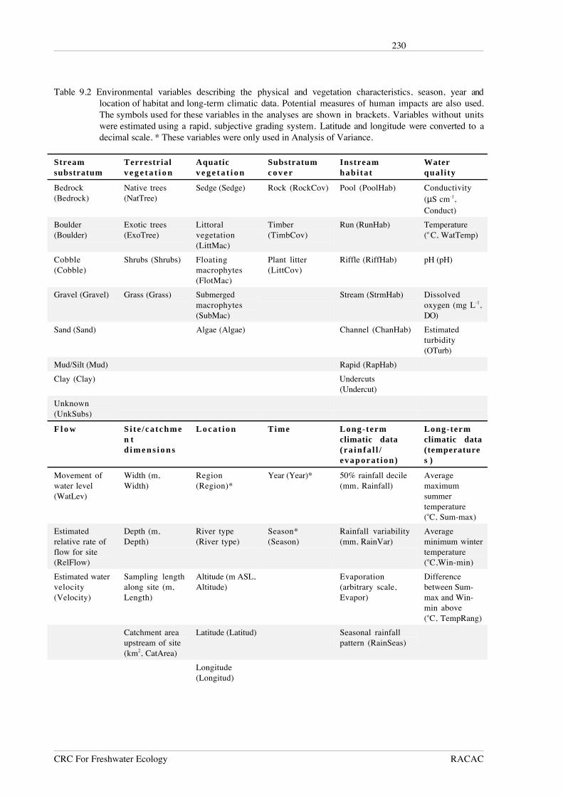
Table 9.2 Environmental variables describing the physical and vegetation characteristics, season, year andlocation of habitat and long-term climatic data. Potential measures of human impacts are also used.The symbols used for these variables in the analyses are shown in brackets. Variables without unitswere estimated using a rapid, subjective grading system. Latitude and longitude were converted to adecimal scale. * These variables were only used in Analysis of Variance.
Streamsubstratum
Terrestrialv e g e t a t i o n
Aquaticv e g e t a t i o n
Substratumc o v e r
Instreamhabi ta t
Waterqual i ty
Bedrock(Bedrock)
Native trees(NatTree)
Sedge (Sedge) Rock (RockCov) Pool (PoolHab) Conductivity(µS cm-1,Conduct)
Boulder(Boulder)
Exotic trees(ExoTree)
Littoralvegetation(LittMac)
Timber(TimbCov)
Run (RunHab) Temperature(o C, WatTemp)
Cobble(Cobble)
Shrubs (Shrubs) Floatingmacrophytes(FlotMac)
Plant litter(LittCov)
Riffle (RiffHab) pH (pH)
Gravel (Gravel) Grass (Grass) Submergedmacrophytes(SubMac)
Stream (StrmHab) Dissolvedoxygen (mg L-1,DO)
Sand (Sand) Algae (Algae) Channel (ChanHab) Estimatedturbidity(OTurb)
Mud/Silt (Mud) Rapid (RapHab)
Clay (Clay) Undercuts(Undercut)
Unknown(UnkSubs)
F l o w Si te / ca tchmen td i m e n s i o n s
L o c a t i o n Time Long-termclimatic data(ra in fa l l /evaporat ion)
Long-termclimatic data(temperatures )
Movement ofwater level(WatLev)
Width (m,Width)
Region(Region)*
Year (Year)* 50% rainfall decile(mm, Rainfall)
Averagemaximumsummertemperature(oC, Sum-max)
Estimatedrelative rate offlow for site(RelFlow)
Depth (m,Depth)
River type(River type)
Season*(Season)
Rainfall variability(mm, RainVar)
Averageminimum wintertemperature(oC,Win-min)
Estimated watervelocity(Velocity)
Sampling lengthalong site (m,Length)
Altitude (m ASL,Altitude)
Evaporation(arbitrary scale,Evapor)
Differencebetween Sum-max and Win-min above(oC, TempRang)
Catchment areaupstream of site(km2, CatArea)
Latitude (Latitud) Seasonal rainfallpattern (RainSeas)
Longitude(Longitud)
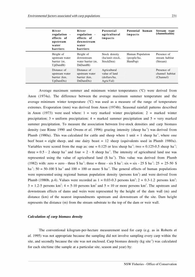
Environmental factors associated with carp populations 231
NSW Fisheries - Office of Conservation
R i v e rregulation -effects ofupstreamwaterbarriers
R i v e rregulation -effects ofdownstreamwaterbarriers
P o t e n t i a lagriculturali m p a c t s
Potential humani m p a c t s
Stream type(channelization)
Height ofupstream waterbarrier (m,UpDamHt)
Height ofdownstreamwater barrier (m,DnDamHt)
Stock density(ha/unit-stock,StockDen)
Human Population(people/ha,HumPop)
Presence ofstream habitat(Stream)
Distance ofupstream waterbarrier (km,UpDamDis)
Distance ofupstream waterbarrier (km,DnDamDis)
Agriculturalvalue of land(dollars/ha,AgricVal)
Presence ofchannel habitat(Channel)
Average maximum summer and minimum winter temperatures (oC) were derived from
Anon (1974a). The difference between the average maximum summer temperature and the
average minimum winter temperature (oC) was used as a measure of the range of temperature
extremes. Evaporation (mm) was derived from Anon (1974b). Seasonal rainfall patterns described
in Anon (1973) were used where: 1 = very marked winter precipitation; 2 = marked winter
precipitation; 3 = uniform precipitation; 4 = marked summer precipitation and 5 = very marked
summer precipitation. To measure the association between live-stock densities and carp biomass
density (see Rinne 1990 and Owens et al. 1996) grazing intensity (sheep ha-1) was derived from
Plumb (1980a). This was calculated for cattle and sheep where 1 unit = 1 sheep ha-1, where one
beef beast = eight sheep, and one dairy beast = 12 sheep (equivalents used in Plumb 1980a).
Variables were scored from the map as: one = 0.125 or less sheep ha-1; two = 0.125-0.5 sheep ha-1;
three = 0.5 - 2 sheep ha-1 and four = 2 - 8 sheep ha-1. The intensity of agricultural land use was
represented using the value of agricultural land ($ ha-1). This value was derived from Plumb
(1982) with: zero = zero - three $ ha-1; three = three - six $ ha-1; six = six - 25 $ ha-1; 25 = 25-50 $
ha-1; 50 = 50-100 $ ha-1 and 100 = 100 or more $ ha-1. The general effects of human populations
were represented using regional human population density (persons km2) and were derived from
Plumb (1980b, p.4). Values were recorded as 1 = 0.03-0.3 persons km2; 2 = 0.3-1.2 persons km2;
3 = 1.2-5 persons km2; 4 = 5-10 persons km2 and 5 = 10 or more persons km2. The upstream and
downstream effects of dams and weirs were represented by the height of the dam wall (m) and
distance (km) of the nearest impoundments upstream and downstream of the site. Dam height
represents the distance (m) from the stream substrate to the top of the dam or weir wall.
Calculation of carp biomass density
The conventional kilogram-per-hectare measurement used for carp (e.g. as in Roberts et
al. 1995) was not appropriate because the sampling did not involve sampling every carp within the
site, and secondly because the site was not enclosed. Carp biomass density (kg site-1) was calculated
for each site/time (the sample at a particular site, season and year) by:
232
CRC For Freshwater Ecology RACAC
Number of carp caught (count) x average weight of measured carp (kg)..................Eqn. 2
Average weight of measured carp at each site was based on the average of individually
calculated fish weights for each site/time combination. Individual calculations of weight were
based on fish fork lengths recorded during the NSW Rivers Survey and the length-weight
regression relationship of carp collected in the study by Gehrke et al. (1995). This was based on
7109 carp individuals collected from the Paroo, Darling, Murrumbidgee and Murray Rivers (r2 =
0.9881; df = 1, 7107; F = 591874.253; p < 0.001). The length-weight equation used was:
ln (weight (g)) = -10.813 + 3.077 ln (fork length (mm))..........................................Eqn. 3
Fork length (mm) was converted into ln (weight (g)) using equation 3, and then weight
(kg). This value for weight (kg) was then used in equation 2.
Analyses
The relationship between carp biomass density and habitat in New South Wales
For all analyses where a relationship with carp biomass density was tested the following
expression was used to transform carp biomass density: (kg site-1)
‘Carp biomass density’ = log10 (carp biomass density (kg site-1) + 2.3)..................Eqn. 4
This transformation increased the homogeneity of variance, as assessed by using residual
plots, and the normality of the distribution as measured by the Shapiro-Wilks statistic; thereby
reducing the type I error rate (SAS Institute 1990). The use of a constant in this transformation
was necessary to avoid attempting to calculate a logarithm of zero at sites without carp. The
constant represents the average weight of a carp in the New South Rivers Survey (2.293 kg).
Spatial and temporal scales of variation in carp biomass density
To determine the spatial and temporal scales at which most variation in carp biomass
density occurs, Analyses of Variance (ANOVA) using a fully crossed and balanced design were
performed (SAS Institute 1990). Temporal effects (year and season) were only analysed to check
if they should be considered as confounding effects on the spatial distribution of carp biomass
density. This was initially done using the factors: region, river class, year and season (see
Chapter 1 for explanations of region and river class). Regions found to be not significantly
different, using ANOVA and the Tukey-Kramer procedure for unplanned comparisons of means
(SAS Institute 1990, hereafter collectively referred to as the Tukey-Kramer test), were pooled and
the variance of carp biomass density was tested using factors: river type, year and season.
Environmental factors associated with carp populations 233
NSW Fisheries - Office of Conservation
(“Significant” indicates α = 0.05 hereafter unless otherwise stated). The Tukey-Kramer test
controls the rate of Type I error when comparing many treatments (e.g. river type).
The effects of large dams
The dam wall height and distance from the site of dams, both upstream and downstream,
were used for all coastal-river analyses, and with the use of all correlation matrices. However, with
stepwise regression and Discriminant Function Analysis (DFA, SAS Institute 1990) applied to the
inland rivers data (discussed below), dam height was not used as a variable in the initial analysis,
for either upstream or downstream dams, because of missing values (8 and 32 missing values out
of 120 respectively).
Environmental factors associated with carp presence
To describe the environmental variables that may discriminate between sites with and
without carp, stepwise DFA was used. Stepwise DFA removes autocorrelated variables from the
model. Variables with a high F-value, including those removed because of autocorrelation, were
used in alternative (non-stepwise) DFA models for predicting carp presence. This DFA model was
tested using the cross-validation procedure for DFA in SAS (SAS Institute 1990). This runs the
DFA on a subset of the data and validates the model with the rest of the data. Each prediction of a
site to a group (either ‘carp’ or ‘no carp’), using the DFA model, was calculated separately thus
giving unbiased discrimination. Montane sites (sites higher than 700 m ASL) were not included in
these analyses because we considered the processes that exclude carp from montane sites (e.g.
migration barriers, high water velocity) could be very different to those excluding carp in lower-
altitude sites.
In addition, to explore what factors may physically exclude carp in montane sites, or what
makes montane habitat unsuitable for carp (e.g. lack of fine sediment), differences betwen
montane and non-montane sites were tested. This involved using ANOVA and the Tukey-Kramer
test 21 times so the significance level of α = 0.05 was adjusted to α = 0.0024 in accordance with
the Dunn-Sidak correction suggested in Sokal and Rohlf (1981).
Environmental gradients over which carp biomass density varies
The habitat factors related to carp biomass density within regions, in non-montane sites,
were determined using multiple stepwise regression (SAS Institute 1990). A correlation matrix,
using Pearson product-moment correlations (SAS Institute 1990), was also used to identify
variables significantly ( r ≥ 0.3) correlated with carp biomass density, including those variables
removed because of colinearity during stepwise regression. Regions that were not significantly
different in carp biomass density in the ANOVA procedures were pooled for analyses (e.g. the
234
CRC For Freshwater Ecology RACAC
Murray and Darling regions). Outliers in the regressions considered to have a disproportionate
effect on the regression line, as assessed using the Cooks D statistic (SAS Institute 1990), were
removed. Montane sites were not included in these analyses. As no carp were caught in them
(Harris et al. 1995) they would have created unnecessary ‘noise’ in the analyses. The change in
the average weight of carp and the carp catch along an altitudinal gradient in non-montane inland
New South Wales was also tested with linear regression (SAS Institute 1990).
RESULTS
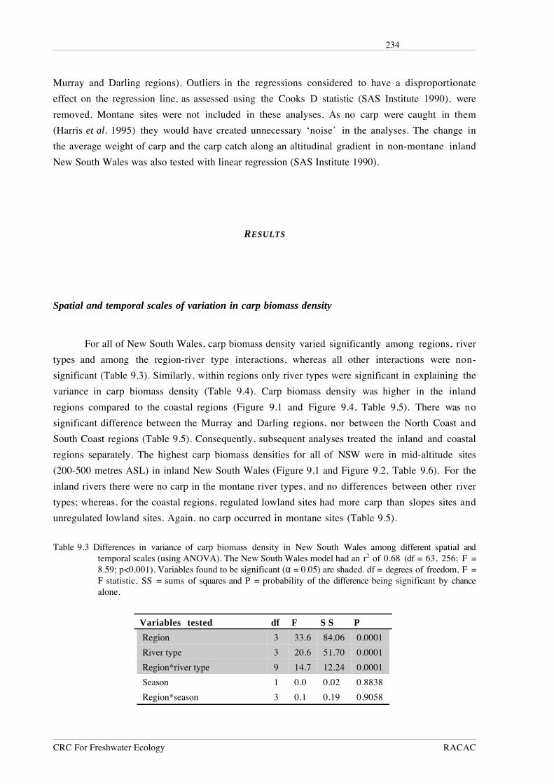
Spatial and temporal scales of variation in carp biomass density
For all of New South Wales, carp biomass density varied significantly among regions, river
types and among the region-river type interactions, whereas all other interactions were non-
significant (Table 9.3). Similarly, within regions only river types were significant in explaining the
variance in carp biomass density (Table 9.4). Carp biomass density was higher in the inland
regions compared to the coastal regions (Figure 9.1 and Figure 9.4, Table 9.5). There was no
significant difference between the Murray and Darling regions, nor between the North Coast and
South Coast regions (Table 9.5). Consequently, subsequent analyses treated the inland and coastal
regions separately. The highest carp biomass densities for all of NSW were in mid-altitude sites
(200-500 metres ASL) in inland New South Wales (Figure 9.1 and Figure 9.2, Table 9.6). For the
inland rivers there were no carp in the montane river types, and no differences between other river
types; whereas, for the coastal regions, regulated lowland sites had more carp than slopes sites and
unregulated lowland sites. Again, no carp occurred in montane sites (Table 9.5).
Table 9.3 Differences in variance of carp biomass density in New South Wales among different spatial andtemporal scales (using ANOVA). The New South Wales model had an r2 of 0.68 (df = 63, 256; F =8.59; p<0.001). Variables found to be significant (α = 0.05) are shaded. df = degrees of freedom, F =F statistic, SS = sums of squares and P = probability of the difference being significant by chancealone.
Variables tested df F S S P
Region 3 33.6 84.06 0.0001
River type 3 20.6 51.70 0.0001
Region*river type 9 14.7 12.24 0.0001
Season 1 0.0 0.02 0.8838
Region*season 3 0.1 0.19 0.9058
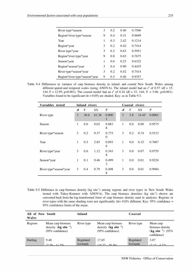
Environmental factors associated with carp populations 235
NSW Fisheries - Office of Conservation
River type*season 3 0.2 0.40 0.7560
Region*river type*season 9 0.4 0.31 0.9699
Year 1 0.3 2.42 0.1214
Region*year 3 0.2 0.42 0.7414
River type*year 3 0.3 0.63 0.5951
Region*river type*year 9 0.8 0.63 0.7675
Season*year 1 0.0 0.23 0.6322
Region*season*year 3 0.4 0.90 0.4435
River type*season*year 3 0.2 0.42 0.7414
Region*river type*season*year 9 0.5 0.40 0.9357
Table 9.4 Differences in variance of carp biomass density in inland, and coastal New South Wales amongdifferent spatial and temporal scales (using ANOVA). The inland model had an r2 of 0.57 (df = 15,144; F = 12.95; p<0.001). The coastal model had an r2 of 0.24 (df = 15, 144; F = 3.06; p<0.001).Variables found to be significant (α = 0.05) are shaded. Key: as in Table 9.3.
Variables tested Inland rivers Coastal rivers
df F SS P df F SS P
River type 3 30.6 61.36 0.0001
3 3.8 14.45 0.0001
Season 1 0.0 0.02 0.8838
1 0.0 0.00 0.9575
River type*season 3 0.2 0.37 0.7750
3 0.2 0.74 0.5313
Year 1 0.5 2.85 0.0936
1 0.0 0.15 0.7007
River type*year 3 0.6 1.12 0.3438
3 0.0 0.07 0.9755
Season*year 1 0.1 0.46 0.4993
1 0.0 0.01 0.9224
River type*season*year 3 0.4 0.79 0.4988
3 0.0 0.01 0.9984
Table 9.5 Difference in carp biomass density (kg site-1) among regions and river types in New South Wales(tested with Tukey-Kramers with ANOVA). The carp biomass densities (kg site-1) shown areconverted back from the log-transformed form of carp biomass density used in analyses. Regions orriver types with the same shading were not significantly (α= 0.05) different. Key: 95% confidence =95% confidence limits of the mean.
All of New SouthWales
Inland Coastal
Regions Mean carp biomassdensity (kg site -1)(95% confidence)
River type Mean carp biomassdensity (kg site -1)(95% confidence)
River type Mean carpbiomass density(kg site -1) (95%confidence)
Darling 9.40
(7 79 - 11 25)
Regulatedlowlands
17.65
(15 27 - 20 36)
Regulatedlowlands
3.07
(2 12 - 4 22)
236
CRC For Freshwater Ecology RACAC
Murray 11.89
(9 81 14 33)
Unregulatedlowlands
18.21
(15 56 21 26)
Unregulatedlowlands
0.0
(0 00 0 00)North coast 0.56
(0 32 - 0 82)
Slopes 27.01
(21 05 - 36 79)
Slopes 0.26
(0 07 - 0 46)South coast 0.69
(0 46 - 0 93)
Montane 0.0
(0 00 - 0 00)
Montane 0.0
(0 00 - 0 00)
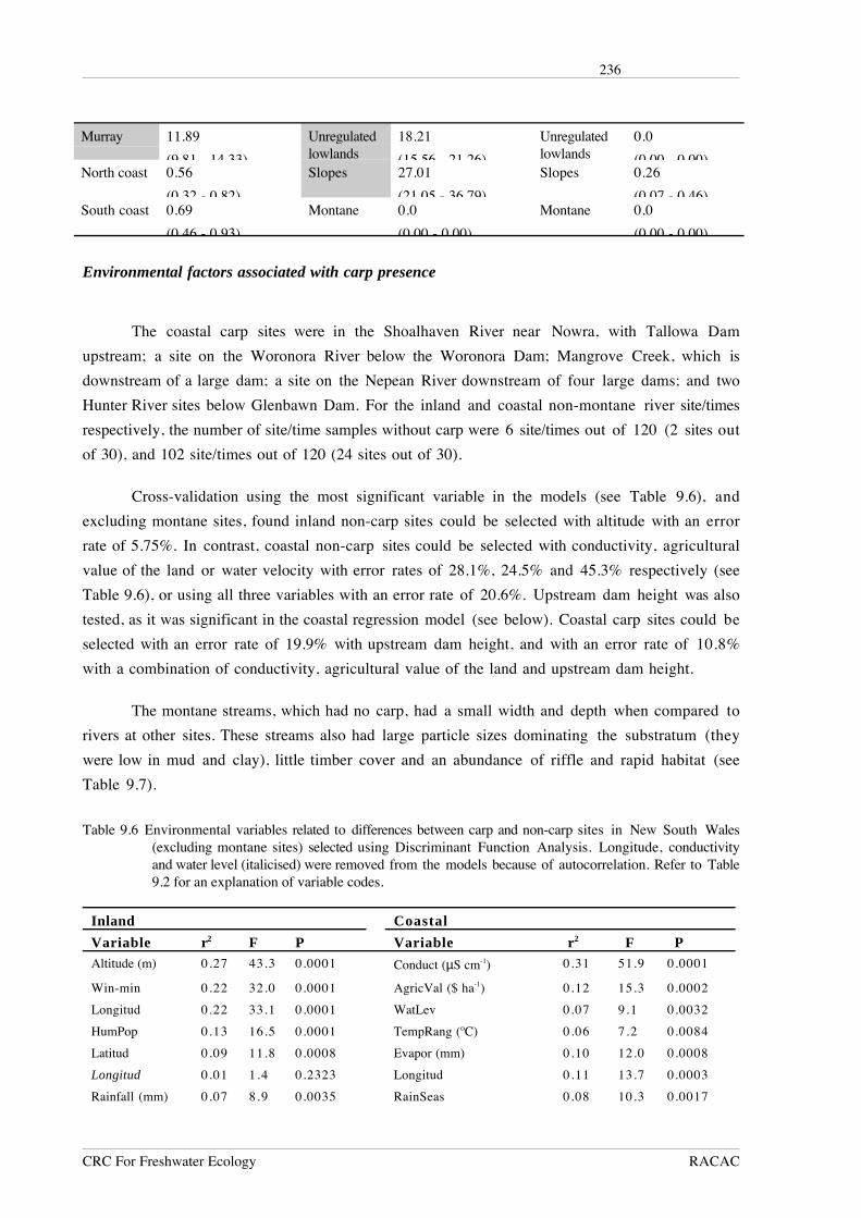
Environmental factors associated with carp presence
The coastal carp sites were in the Shoalhaven River near Nowra, with Tallowa Dam
upstream; a site on the Woronora River below the Woronora Dam; Mangrove Creek, which is
downstream of a large dam; a site on the Nepean River downstream of four large dams; and two
Hunter River sites below Glenbawn Dam. For the inland and coastal non-montane river site/times
respectively, the number of site/time samples without carp were 6 site/times out of 120 (2 sites out
of 30), and 102 site/times out of 120 (24 sites out of 30).
Cross-validation using the most significant variable in the models (see Table 9.6), and
excluding montane sites, found inland non-carp sites could be selected with altitude with an error
rate of 5.75%. In contrast, coastal non-carp sites could be selected with conductivity, agricultural
value of the land or water velocity with error rates of 28.1%, 24.5% and 45.3% respectively (see
Table 9.6), or using all three variables with an error rate of 20.6%. Upstream dam height was also
tested, as it was significant in the coastal regression model (see below). Coastal carp sites could be
selected with an error rate of 19.9% with upstream dam height, and with an error rate of 10.8%
with a combination of conductivity, agricultural value of the land and upstream dam height.
The montane streams, which had no carp, had a small width and depth when compared to
rivers at other sites. These streams also had large particle sizes dominating the substratum (they
were low in mud and clay), little timber cover and an abundance of riffle and rapid habitat (see
Table 9.7).
Table 9.6 Environmental variables related to differences between carp and non-carp sites in New South Wales(excluding montane sites) selected using Discriminant Function Analysis. Longitude, conductivityand water level (italicised) were removed from the models because of autocorrelation. Refer to Table9.2 for an explanation of variable codes.
Inland Coastal
Variable r2 F P Variable r2 F PAltitude (m) 0.27 43.3 0.0001 Conduct (µS cm-1) 0.31 51.9 0.0001
Win-min 0.22 32.0 0.0001 AgricVal ($ ha-1) 0.12 15.3 0.0002
Longitud 0.22 33.1 0.0001 WatLev 0.07 9.1 0.0032
HumPop 0.13 16.5 0.0001 TempRang (ºC) 0.06 7.2 0.0084
Latitud 0.09 11.8 0.0008 Evapor (mm) 0.10 12.0 0.0008
Longitud 0.01 1.4 0.2323 Longitud 0.11 13.7 0.0003
Rainfall (mm) 0.07 8.9 0.0035 RainSeas 0.08 10.3 0.0017
Environmental factors associated with carp populations 237
NSW Fisheries - Office of Conservation
DnDamDis (km) 0.07 8.5 0.0043 WatLev 0.01 0.7 0.4227
Latitud 0.05 5.6 0.0199
Conduct(µS cm-1) 0.03 3.2 0.0774
StockDen (unit-stock ha-1) 0.04 5.2 0.0244
Environmental gradients over which carp biomass density varies
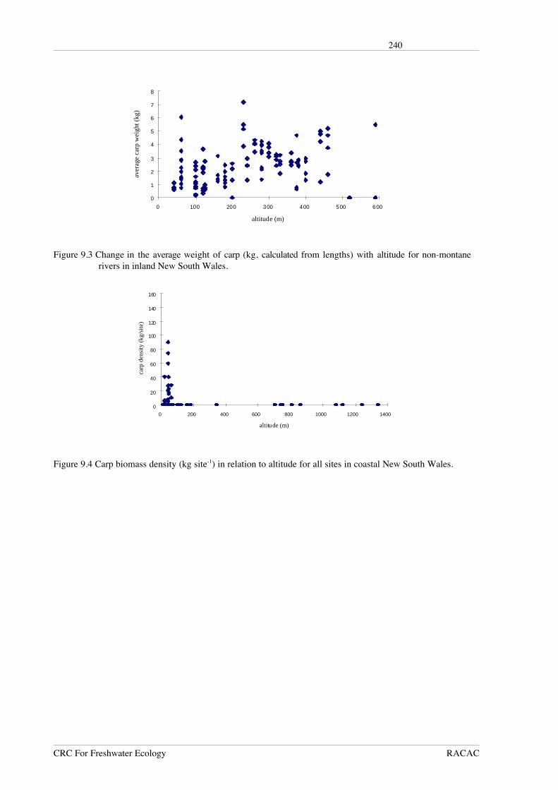
Site altitude was the variable most strongly correlated with carp biomass densities in the
inland regions (stepwise regression and correlation table, Table 9.8 and Table 9.9). The regression
model excluded observations with no carp as these site values - all of which are above 500 m ASL
- each had a Cook’s D value of 0.038. These values had a disproportionate effect on the
regression line, as carp biomass density was progressively higher with altitude up to about 500 m,
beyond which there was only one site with carp (at 600 m, Figure 9.1 and Figure 9.2). The change
in carp biomass density along this altitudinal gradient can be explained by larger average carp
weights (r2 = 0.20; df = 1, 111; F = 27.93; p<0.001) and not a larger carp catch (r2 = 0.001; df =
1, 111; F = 0.13; p>0.05) with higher altitudes in non-montane sites up to 500 m ASL (Figure
9.3). The height of downstream dams was the next most correlated variable with carp biomass
density (Table 9.8, Figure 9.2). The highest carp biomass densities were in mid-altitude sites above
dams or weirs (Table 9.10). High carp biomass density sites also had more riffle habitat, and had a
substratum with more coarse particles (boulders, gravel and rocks) but fewer fine particles such as
clay. These habitats also had smaller catchment areas upstream and lower average winter minimum
temperatures, lower evaporation and higher rainfall (Table 9.9).
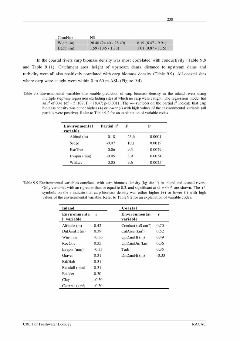
Table 9.7 Environmental factors describing the physical habitat of montane sites versus non-montane sites.Shaded variables are those significantly different at α =0.0024 (which corrects for the increased type Ierror rate with multiple tests). NS = not significantly different at α =0.05.
Variable Mean (95% confidence)
Non-montane sites Montane sites
Boulder NSCobble NSBedrock 1.25 (1.07 - 1.43) 1.81 (1.45 - 2.17)Gravel 1.60 (1.40 - 1.80) 2.13 (1.81 - 2.45)Sand 1.96 (1.76 - 2.16) 2.36 (2.04 - 2.68)Mud 2.30 (2.10 - 2.50) 1.68 (1.34 - 2.02)Clay 1.05 (0.85 - 1.25) 0.30 (0.08 - 0.52)RockCov 1.89 (1.69 - 2.09) 2.38 (2.06 - 2.70)TimbCov 2.72 (2.60 - 2.84) 1.65 (1.41 - 1.89)PlantLitt NSUndercut 1.60 (1.46 - 1.74) 2.03 (1.79 - 2.27)RunHab 0.97 (0.79 - 1.15) 1.51 (1.17 - 1.85)RiffHab 1.23 (1.05 - 1.41) 1.85 (1.59 - 2.11)RapHab 0.18 (0.10 - 0.26) 0.75 (0.47 - 1.03)PoolHab NSStrmHab NS
238
CRC For Freshwater Ecology RACAC
ChanHab NSWidth (m) 26.40 (24.40 - 28.40) 8.19 (6.47 - 9.91)Depth (m) 1.59 (1.45 - 1.73) 1.01 (0.87 - 1.15)
In the coastal rivers carp biomass density was most correlated with conductivity (Table 9.9
and Table 9.11). Catchment area, height of upstream dams, distance to upstream dams and
turbidity were all also positively correlated with carp biomass density (Table 9.9). All coastal sites
where carp were caught were within 0 to 60 m ASL (Figure 9.4).
Table 9.8 Environmental variables that enable prediction of carp biomass density in the inland rivers usingmultiple stepwise regression excluding sites at which no carp were caught. The regression model hadan r2 of 0.41 (df = 5, 107; F = 18.47; p<0.001) . The +/- symbols on the partial r2 indicate that carpbiomass density was either higher (+) or lower (-) with high values of the environmental variable (allpartials were positive). Refer to Table 9.2 for an explanation of variable codes.
Environmentalvariable
Partial r2 F P
Altitud (m) 0.18 23.6 0.0001
Sedge -0.07 10.1 0.0019
ExoTree -0.06 9.3 0.0029
Evapor (mm) -0.05 8.9 0.0034
WatLev 0.05 9.6 0.0025
Table 9.9 Environmental variables correlated with carp biomass density (kg site -1) in inland and coastal rivers.Only variables with an r greater than or equal to 0.3, and significant at α = 0.05 are shown. The +/-symbols on the r indicate that carp biomass density was either higher (+) or lower (-) with highvalues of the environmental variable. Refer to Table 9.2 for an explanation of variable codes.
Inland Coastal
Environmental variable
r Environmentalvariable
r
Altitude (m) 0.42 Conduct (µS cm-1) 0.70
DnDamHt (m) 0.39 CatArea (km2) 0.52
Win-min -0.36 UpDamHt (m) 0.49
RocCov 0.35 UpDamDis (km) 0.36
Evapor (mm) -0.35 Turb 0.35
Gravel 0.31 DnDamHt (m) -0.33
RiffHab 0.31
Rainfall (mm) 0.31
Boulder 0.30
Clay -0.30
CatArea (km2) -0.30

Environmental factors associated with carp populations 239
NSW Fisheries - Office of Conservation
0
20
40
60
80
100
120
140
160
0 200 400 600 800 1000 1200 1400
altitude (m)
carp
den
sity
(kg
/site
)
Figure 9.1 Carp biomass density (kg site-1) in relation to altitude for all sites in inland New South Wales. Apossible threshold, possibly representing environmental conditions unsuitable for carp, is shownstarting at 600 m.
-0.5
0
0.5
1
1.5
2
2.5
3
3.5
4
0-99 100-199 200-299 300-399 400-499
altitude (m)
aver
age
stan
dard
ised
sca
le
carp density (kg/site) DnDamHt Gravel(kg site-1
)
Figure 9.2 Means of carp biomass density (kg site-1), downstream dam height (m, DnDamHt) and abundance ofgravel (Gravel) in the substratum of the inland rivers at different categories of altitude in sites wherecarp were caught. Means of variables for each altitude category were divided by the overall mean forthat variable so relative trends could be illustrated. Error bars indicate 95% confidence limits of themeans.
240
CRC For Freshwater Ecology RACAC
0
1
2
3
4
5
6
7
8
0 100 200 300 400 500 600
altitude (m)
ave
rage
car
p w
eigh
t (kg
)
Figure 9.3 Change in the average weight of carp (kg, calculated from lengths) with altitude for non-montanerivers in inland New South Wales.
0
20
40
60
80
100
120
140
160
0 200 400 600 800 1000 1200 1400
altitude (m)
carp
den
sity
(kg
/site
)
Figure 9.4 Carp biomass density (kg site-1) in relation to altitude for all sites in coastal New South Wales.

Environmental factors associated with carp populations 241
NSW Fisheries - Office of Conservation
Table 9.10 The eight inland sites (out of 40) that had carp densities above 90 kg site-1 and the wall height (m)and distance (km) of the closest upstream and downstream dams. Each site was sampled four times soa biomass density greater than 90 kg site-1 could occur more than once. ‘?‘ indicates that the valuewas unknown.
Sitecode
Carpbiomassdensity
(kg site -1)
River Damupstream
Distancefrom site(km)
Wallheight(m)
Dam downstream Distancefrom site(km)
Wallheight(m)
MS31 155.3 Lachlan None Wyangala 95 82
MRL28 142.7 Tumut Blowering 20 30 Berembed weir 500 3
DS11 135.6 Peel Keepit 18 55 Paradise weir 32 ?
DS13 96.7/132.4 Talbragar None Narromine weir 150 4
MS32 109.4/93.6 Goodradigbee None Burrinjuck 25 80
DUL19 97.7 Bogan None Nyngan Weir 10 3
DS15 96.0/96.5 Horton None Tareelaroi 115 ?
MS34 105.5 Abercrombie None Wyangala 53 82
DS11
DS13
DS15
DUL19
MRL28
MS31
MS32
MS34
NCRL47
NCS54
SCRL66
SCRL67
SCRL69
SCRL70
50 0 100
Scale (km)
Darling
Murray
Nor
th c
oast
Sou
th c
oast
Figure 9.5 The NSW Rivers Survey sites where the highest carp biomass densities (kg site-1) were recorded inNew South Wales. The coastal sites marked represent the only sites where carp were found. Theinland sites marked represent the eight sites (out of 40) which had carp densities above 90 kg site-1.
242
CRC For Freshwater Ecology RACAC
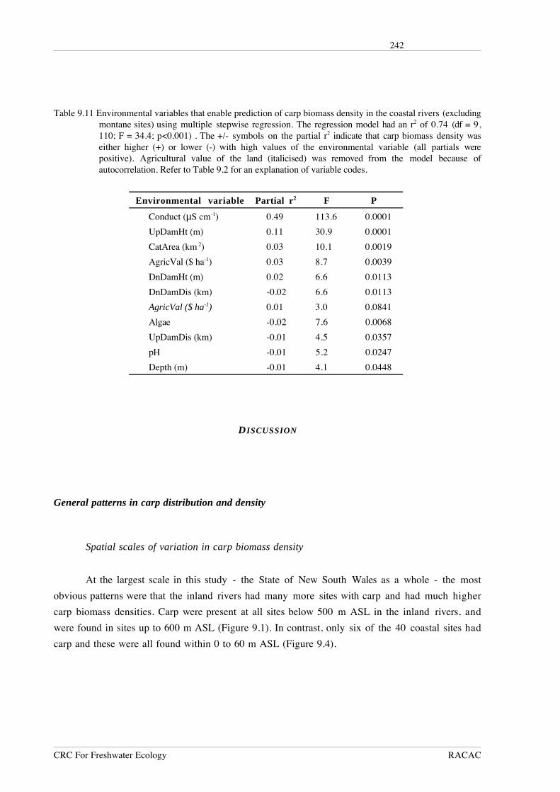
Table 9.11 Environmental variables that enable prediction of carp biomass density in the coastal rivers (excludingmontane sites) using multiple stepwise regression. The regression model had an r2 of 0.74 (df = 9,110; F = 34.4; p<0.001) . The +/- symbols on the partial r2 indicate that carp biomass density waseither higher (+) or lower (-) with high values of the environmental variable (all partials werepositive). Agricultural value of the land (italicised) was removed from the model because ofautocorrelation. Refer to Table 9.2 for an explanation of variable codes.
Environmental variable Partial r2 F P
Conduct (µS cm-1) 0.49 113.6 0.0001
UpDamHt (m) 0.11 30.9 0.0001
CatArea (km 2) 0.03 10.1 0.0019
AgricVal ($ ha-1) 0.03 8.7 0.0039
DnDamHt (m) 0.02 6.6 0.0113
DnDamDis (km) -0.02 6.6 0.0113
AgricVal ($ ha-1) 0.01 3.0 0.0841
Algae -0.02 7.6 0.0068
UpDamDis (km) -0.01 4.5 0.0357
pH -0.01 5.2 0.0247
Depth (m) -0.01 4.1 0.0448
DISCUSSION
General patterns in carp distribution and density
Spatial scales of variation in carp biomass density
At the largest scale in this study - the State of New South Wales as a whole - the most
obvious patterns were that the inland rivers had many more sites with carp and had much higher
carp biomass densities. Carp were present at all sites below 500 m ASL in the inland rivers, and
were found in sites up to 600 m ASL (Figure 9.1). In contrast, only six of the 40 coastal sites had
carp and these were all found within 0 to 60 m ASL (Figure 9.4).
Environmental factors associated with carp populations 243
NSW Fisheries - Office of Conservation
How big were the carp biomass densities?
A very coarse estimate of what the carp biomass densities may indicate in terms of
kilograms per hectare can be derived from the calibration experiment on the Bogan River
(Chapter 3). The first day’s sampling, equivalent to one river survey sample, yielded 30.1 kg site-1.
The density estimate from a subsequent five days’ sampling the same site is 147 kg site-1,
equivalent to 609.5 kg ha-1; (values from Dennis Reid, NSW Fisheries Research Institute). It is very
unlikely that a simple linear relationship to generalise between the biomass density of the carp
caught and the actual biomass density of carp can be accurately used because of variation in catch
efficiency due to factors such as fish size, habitat variation, etc. At least for the Bogan River site,
catch efficiency (i.e. the ratio of Rivers Survey biomass density, 30.1 kg site-1, to total estimated
biomass density, 609.5 kg ha-1) was approximately 1:20. Assuming there was a similar catch
efficiency in the Lachlan River site (Table 9.10) where the highest carp biomass density was
recorded during the NSW Rivers Survey, the carp were at a biomass density of about 3144 kg ha-1.
Environmental factors associated with carp presence and carp biomass densities
The importance of slow-flowing habitat
One of the principal findings of this study is that carp are strongly associated with the
lower altitudes of New South Wales (Figure 9.1 and Figure 9.4). Similarly, large spatial scale
research on fish communities in North America has found carp to predominantly occupy lower
altitudes (e.g. Rahel and Hubert 1991; Brown and Coon 1994; Lyons 1996). Comparisons
between numerous general observations or research results across different altitudes also suggest
that carp predominantly occupy low altitudes in Australia (Brown 1996; McDowall 1996) and in
North America (McCrimmon 1968; Panek 1987). Lowland sites provide breeding habitat in the
form of floodplains, backwaters, shallow river edges and billabongs, all of which are more
prevalent in low altitude sites (Warner 1987; Schumm 1988). These lowland habitats would also be
subject to fewer periodic or episodic high-velocity flows. The high biomass densities of carp in the
inland rivers can be partly explained by the greater availability of lowland habitat that provides
suitable slow-flowing spawning grounds and nursery areas for carp. For most of their length the
inland rivers are dominated by low-gradient, low-velocity habitat at low altitudes (Warner 1987).
In contrast, the coastal rivers have very short sections with low gradients (Warner 1987).
The absence of carp from the 20 montane sites sampled may have been due to the lack of
access to slow-flowing habitat. The montane streams are characterised by small channels, high
gradients, frequent rapids and riffles, large substrate particles and few deep areas (Table 9.7).
They are erosive zones rather than the depositional floodplain habitats favoured by carp. These
streams would have little habitat in which carp could spawn or take refuge from high flows. The

244
CRC For Freshwater Ecology RACAC
combination of these unsuitable conditions and the presence of barriers, both natural (waterfalls)
and artificial (dams and weirs), blocking upstream dispersal from the original lower-Murray
source of Boolara carp in the inland rivers (Davis 1977) would have excluded carp from many
montane sites.
In spite of the importance of low-velocity flows to carp spawning, conditions indicating
low energy flows were not consistently associated with high carp biomass densities. The highest
carp biomass densities were found in association with conditions indicating high-energy flows
(coarse substrate) in mid-altitude sites in the inland rivers, and yet carp in the coastal rivers were
found in association with high conductivity and low altitudes which suggest low-energy flows
(Table 9.9 and Table 9.11). Conductivity is a coarse measure of chemical richness (Welcomme
1979), and therefore can be higher at low flows because salts leaching into the stream from the
water table become more concentrated (Lawrence et al. 1981; Metzeling et al. 1995). Velocity
was not a significant variable (Table 9.2, Table 9.8 - Table 9.11) possibly because critical high
flows detrimental to carp were poorly represented over time, as only four measurements were
taken per site, two during a drought, and field sampling was scheduled to avoid floods.
Furthermore, within the lowland reaches of both the inland and coastal rivers, breeding sites of
carp would have largely been in the slow-flowing backwaters and billabongs, which were not
sampled. However, these limitations in sampling do not explain the conflicting results between the
coastal and inland rivers. These conflicting results could be expected if adults from self-sustaining
carp populations were able to migrate into high-altitude, high-energy flow habitat. For the inland
rivers the breeding populations of carp may have been within the lower altitudes (below 200 m
ASL) or in downstream water storages (Table 9.10) Low carp recruitment at high altitudes was
indicated by the small proportion of fish less than 1kg above an altitude of 200 m ASL (Figure
9.3), suggesting also that the dense carp populations found in mid-altitude sites consist of adult
fish recruiting from downstream reaches and migrating upstream. Carp length-frequency
distributions for the Darling River, Bogan River and Little River (Chapter 2) also show clear
increases in average size with increasing altitude. The higher altitude populations would have
resulted from the strong upstream migration that has been documented for adult carp (Mallen-
Cooper et al. 1995). These results indicate that viable high biomass density carp populations of
high biomass density do not require the conditions associated with low-energy flows and fine
substrata if they are maintained by migration from downstream breeding populations.
Human impacts and carp
The human impact most clearly indicated as an effect on carp in this study was flow
regulation. The heights of dam (or weir) walls in New South Wales, upstream of coastal sites, and
downstream of inland sites, were positively correlated with carp biomass densities (Table 9.8, Table
9.9, Table 9.11, Figure 9.2). In addition, carp were only found in regulated lowland rivers in the
coastal region (Figure 9.5). Large larger dams usually result in greatly altered flow variability and,
Environmental factors associated with carp populations 245
NSW Fisheries - Office of Conservation
for sites downstream of most dams, summer water temperatures are suppressed (Cadwallader 1978;
Faragher and Harris 1984). Such changes in flow and temperature are suitable for adult carp but
not for native fish (Harris 1997; Gehrke et al. 1995, Chapter 4). The direction (upstream or
downstream) of the carp sites relative to these dams reflected the location of higher carp biomass
densities. Large-biomass populations were in higher altitudes (200-500 m ASL) in the inland
rivers both upstream and downstream of large dams (Table 9.10) but only in the lower altitudes of
the coast. The positive correlation between coastal carp biomass densities and distance from
upstream dams (Table 9.9) is likely to be an artefact of natural barriers to upstream migration of
carp, and associated with the scarcity of regulated reaches in coastal lowland rivers and their
invariable occurrence near sea level.
This association between large dams and carp was more evident in the inland rivers,
probably reflecting a greater impact. As well as having more habitat area which supports carp, the
flows of major inland rivers are also more intensely modified to provide water for irrigation, as
opposed to the coastal dams which are mainly for municipal water supply (Chapter 7). These
results also reflected the association between fish communities dominated by carp and the more-
regulated inland New South Wales rivers found by Gehrke et al. (1995). In the inland rivers, dams
have prevented upstream migration of native fish, thereby affecting fish-community composition
in the mid-altitudes (Mallen-Cooper et al. 1995; Harris and Mallen-Cooper 1994). Large carp
biomass densities would have resulted from carp travelling upstream and congregating beneath
dams such as Keepit Dam and Blowering Dam (Table 9.10). The passage of migrating carp may
also have been blocked by natural barriers such as waterfalls. Inland rivers upstream of many
dams are also suitable for carp (e.g. sites in Table 9.10). Upstream of dams, where the largest carp
biomass densities occurred (Figure 9.2), abundant carp populations breeding in water storages
may also have affected upstream fish communities. Dam construction in the United States of
America led to increases in carp numbers in the storages of these dams (Hoyt and Robison 1980;
Winston et al. 1991). These American carp populations are said to proliferate in impoundments
and then move upstream in large numbers (Winston et al. 1991). Artificial lakes such as Lake
Burley Griffin in the Australian Capital Territory that have a high proportion of carp in the fish
catch (Lintermans 1996) may also supplement carp biomass densities in inflowing rivers by
upstream migration.
The relative importance of natural effects and human impacts is difficult to discern for the
coastal rivers, as carp populations, conditions indicating low-energy flows (low altitude and higher
conductivity), rivers with large upstream dams, and greater agricultural use were all found along a
narrow coastal strip (Table 9.9, Table 9.11). The more important human impacts are also not
clear, In the six coastal sites in which carp were present the agricultural value of land was high and
the upstream dams were large. The high conductivities also give some indication of water quality
in coastal carp habitats. These rivers could be chemically enriched by reduced or naturally low
flows which can lead to a greater mixing of salts with the water table (Lawrence et al. 1981;
Metzeling et al. 1995). High conductivity could also indicate increased input of sediments and
246
CRC For Freshwater Ecology RACAC
dissolved solids from catchment modification associated with agriculture. A greater chemical
richness could also result from other human activities. For example, nutrient loading from human
treated sewage affects the Hawkesbury-Nepean River and has caused a marked change in the fish
community and increased carp abundance (Pollard et al. 1994).
It is possible that flow regulation and agriculture played a more equal role in affecting
carp biomass densities than this study indicates. The association between areas of high agricultural
value and high carp biomass densities may also have been found in the inland rivers if adult carp
were unable to migrate upstream from spawning sites. Agricultural land use and the resulting
ecological effects have been often been documented for southeastern Australia (Cadwallader
1978; Koehn and O’Connor 1990; Faragher and Harris 1994; Metzeling et al. 1995; Brierley et
al. 1996; Finlayson and Silburn 1996; Ogden 1996). These disturbances generally lead to a
decline in native species and an increase in alien species such as carp (Harris 1997; Arthington et
al. 1989).
CONCLUSION
This study indicates that carp were suited by conditions that existed before European
settlement, but also that flow regulation and activities associated with agricultural land use lead to
higher carp biomass densities. The association with flow regulation was more evident in the inland
rivers, where carp are more widespread. The modification of water temperatures and flow
variability by dams would have reduced the size of native fish populations and increased the
abundance of carp. Carp populations breeding in water storages behind, and also in lowland
habitats (less than 200 m ASL) probably maintain some inland carp populations at higher
altitudes (200-500 m ASL) through the upstream migration of adult carp. Barriers to fish
migration, dams and natural barriers, would have blocked these upstream migrations and thereby
created a concentration of carp biomass densities in mid-altitude sites. These high-biomass density
populations were also associated with conditions indicating high-energy flows such as coarse
substrate, suggesting that carp populations can be maintained in sub-optimal habitat through adult
migration. For the coastal rivers the relative importance of different human impacts on carp
biomass density was difficult to discern. Carp populations, conditions indicating low-energy flows,
river reaches with large upstream dams and land of greater agricultural value were all found along
a narrow coastal strip. The implications of these results are that river management focused on carp
spawning sites, carp migration, the effects of agriculture, and river regulation would be effective in
reducing carp biomass densities, improving water quality and increasing native fish stocks.
Environmental factors associated with carp populations 247
NSW Fisheries - Office of Conservation
ACKNOWLEDGMENTS
We are very grateful for the enormous effort by the Rivers Survey team, in particular,
Simon Hartley and Andrew Bruce. Cathy Hale, University of Canberra, was extremely useful as an
authority for univariate statistics. Ken Thomas, Phillip Sloane, Justen Simpson, Kerry Beggs, Geoff
Gordon and Dennis Reid also provided statistical advice. Peter Gehrke and Craig Schiller allowed
the use of length-weight data. Peter Gehrke, Martin Thoms, Mark Lintermans, Kylie Peterson,
Louisa Oswald, Chris Driver, Marita Sydes, Jane Roberts, Bruce Chessman and the Applied Science
Writers Group gave useful comments on the manuscript. This report was made possible by the
financial support of the New South Wales Resource and Conservation Assessment Council, the
Cooperative Research Centre for Freshwater Ecology, the NSW Fisheries Research Institute and the
University of Canberra.
REFERENCES
Anon (1973). Climate. Atlas of Australian Resources. Second series. Department of Minerals andEnergy, Canberra.
Anon (1974a). Climatic Atlas of Australia, Map Set 1, Temperature. Department of Science,Bureau of Meteorology. Australian Government Publishing Service.
Anon (1974b). Climatic Atlas of Australia, Map Set 3, Evaporation. Department of Science,Bureau of Meteorology. Australian Government Publishing Service.
Arthington, A.H., Hamlet, S. and Bluhdorn, D.R. (1989). The role of habitat disturbance in theestablishment of introduced warm-water fishes in Australia. In ‘Introduced andTranslocated Fishes and their Ecological Effects’. (Ed. D.A. Pollard). (Department ofPrimary Industry and Energy, Bureau of Rural Resources. Proceedings No. 8. AustralianSociety for Fish Biology Workshop). p. 61-66
Balon, E.K. (1974). Domestication of the Carp Cyprinus carpio L. Royal Ontario Museum LifeSciences, Miscellaneous Publication.
Breukelaar, A.W., Lammens, E.H.R.R., Klein Breteler, Jan G.B. and Tatrai, I. (1994). Effects ofbenthivorous bream (Abramis brama) and carp (Cyprinus carpio ) on sedimentresuspension and concentration of nutrients and chlorophyll a. Freshwater Biology 32,113-121.
Brierley, G.J., Fryirs, K. and Cohen, T. (1996). Geomorphology and river ecology in southeasternAustralia: an approach to catchment characterisation. Part one. A geomorphic approachto catchment characterisation. Graduate School of the Environment. Working paper 9603,Macquarie University, Sydney.

248
CRC For Freshwater Ecology RACAC
Brown, D.J. and Coon, T.G. (1994). Abundance and Assemblage Structure of Fish Larvae in theLower Missouri River and its Tributaries. Transactions of the American Fish Society 123,718-732.
Brown, P. (1996). Carp in Australia. Fishfacts 4, (NSW Fisheries, Sydney.)
Bureau of Meterology (1973). Climate. Atlas of Australian Resources. Second series. Departmentof Minerals and Energy, Canberra.
Bureau of Meterology (1974a). Climatic Atlas of Australia, Map Set 1, Temperature. Departmentof Science, Bureau of Meteorology. Australian Government Publishing Service.
Bureau of Meterology (1974b). Climatic Atlas of Australia, Map Set 3, Evaporation. Departmentof Science, Bureau of Meteorology. Australian Government Publishing Service.
Cadwallader, P.L. (1978). Some causes of the decline in range and abundance of native fish in theMurray-Darling river system. Proceedings of the Royal Society of Victoria 90, 211-224.
Crivelli, A.J. (1981). The biology of the common carp, Cyprinus carpio L. in the Camargue,southern France. Journal of Fish Biology 18, 271-290.
Crivelli, A.J. (1983). The destruction of aquatic vegetation by carp. Comparison between SouthernFrance and the United States. Hydrobiologia 106, 37-41.
Cullen, P., Doolan, J., Harris, J., Humphries, P., Thoms, M. and Young, W. (1996). Environmentalallocations - the ecological imperatives. In Managing Australia’s Inland Waters. Roles forScience and Technology. Prime Ministers Science and Engineering Council. Departmentof Industry, Science and Tourism, Canberra.
Davis, K. (1997) Investigations into the genetic variation of the carp, Cyprinus carpio Linnaeus, insouth-eastern Australia. Ph.D. Thesis, University of New South Wales
Faragher, R.A. and Harris, J.H. (1994). The historical and current status of freshwater fish in NewSouth Wales. Australian Zoologist 29, 166-176.
Finlayson, B. and Silburn, M. (1996). Soil, nutrient and pesticide movements from different landuse practices, and subsequent transport by rivers and streams In Downstream Effects ofLand Use, pp. 129-140. Department of Natural Resources, Queensland, Australia.
Fletcher, A.R., Morison, A.K. and Hume, D.J. (1985). Effects of carp, Cyprinus carpio L., onCommunities of Aquatic Vegetation and Turbidity of Waterbodies in the Lower GoulburnRiver Basin. Australian Journal of Marine and Freshwater Research 26, 311-27.
Gehrke, P.C. and Harris, J.H. (1994). The role of fish in cyanobacterial blooms in Australia.Australian Journal of Marrine and Freshwater Research 45, 905-15.
Gehrke, P.C., Brown, P., Schiller, C.B., Moffatt, D.B. and Bruce, A.M. (1995). River regulation andfish communities in the Murray-Darling System, Australia. Regulated Rivers: Researchand Management 11, 363-375
Harris, J. H. (1995). Carp: the prospects for control? Water 22, 25-28.
Harris, J. H., Bruce, A., Davis, K., Hartley, S. and Silveira, R. (1995). Study of the Fish Resourcesof NSW Rivers. First Annual Report, May 1995. NSW Fisheries Research Institute andCooperative Research Center for Freshwater Ecology.
Harris, J.H. (1997). Environmental rehabilitation and carp control. In “Controlling Carp:exploring the options for Australia”. Proceedings of a workshop 22-24 October 1996,Albury. (Roberts, J. and Tilzey, R., Eds.). CSIRO Land and Water, Griffith.

Environmental factors associated with carp populations 249
NSW Fisheries - Office of Conservation
Harris, J.H. and Mallen-Cooper, M. (1994). Fish passage development in the rehabilitation offisheries in mainland south-eastern Australia. Proceedings of the International Symposiumand Workshop on Rehabilitation of Inland Fisheries, Hull, 6-10 April, 1992. (Ed. I.Cowx) pp. 185-193.
Hoyt, R.D. and Robison, W.A. (1980). Effects on impoundment on the fishes in two Kentuckytailwaters. Proceedings of the Annual Conference of the South Eastern Association ofFisheries and Wildlife Agencies 24, 307-317.
Hume, D.J., Fletcher, A.R. and Morison, A.K. (1983). Carp program Final Report. No.10. ArthurRylah Institute for Environmental Research, Fisheries and Wildlife Division, Ministry forConservation, Victoria.
Hume. D.J. and Pribble, H.J. (1980). Carp program. No. 5. The biology and behaviour of carp(Cyprinus carpio): a brief review. Fisheries and Wildlife Division, Ministry forConservation.
King, A. (1995). The effects of carp on aquatic ecosystems - a literature review. A report preparedfor the Environmental Protection Authority NSW, Murray region; November, 1995.
Koehn, J.D. and O’Connor, W.G. (1990). Threats to Victorian native freshwater fish. VictorianNaturalist 107, 5-12.
Lawrence, I., Lansdown, P. and Newsome, H. (1981). Waters of the Canberra Region. MetropolitanPlanning Issues. Technical Paper 30. February 1981. National Capital DevelopmentCommission, Canberra, ACT.
Lee, D.M. and Gaffney, D.O. (1986). District Rainfall Deciles-Australia. MeteorologicalSummary, September 1986. Bureau of Meteorology, Department of Science. AustralianGovernment Publishing Service, Canberra.
Lintermans, M. (1996). The Lake Burley Griffin Fishery - 1996 sampling report. A report to theNational Capital Planning Authority. August 1996. Wildlife Research Unit, ACT Parks andConservation Service.
Lyons, J. (1996). Patterns in the species composition of fish assemblages among Wisconsinstreams. Environmental Biology of Fishes 45: 329-341.
Mallen-Cooper, M., Stuart, I.G., Hides-Pearson, F. and Harris, J.H. (1995). Fish migration in theMurray River and assessment of the Torrumbarry Fishway. Final Report for NaturalResources Management Strategy Project N002. NSW Fisheries Research Institute and theCooperative Research Centre for Freshwater Ecology.
McCrimmon, H.R. (1968). Carp in Canada. Bulletin of the Fisheries Research Board of Canada165. 93 pp.
McDowall, R. (1996). Freshwater Fishes of South-eastern Australia. A.H. and A.W. Reed Pty Ltd.,Sydney.
Metzeling, L., Doeg, T. and O’Connor, W. (1995). The impact of salinization and sedimentationon aquatic biota. In ‘Conserving Biodiversity: Threats and Solutions. (Eds R.A. Bradstock,T.D. Auld, D.A. Keith, R.T. Kingsford, D. Lunney and D.P. Sivertson.) pp. 126-136(Surrey Beatty and Sons.)
Ogden, R. (1996). Potential for the restoration of aquatic macrophytes in billabongs. in “FirstNational Conference on Stream Management in Australia”. Merrijig 19-23 February1996. (I. Rutherford and M. Walker, Eds.).
Owens, L.B., Edwards, W.W., and Van Keuren, R.W. (1996). Sediment losses from a pasturedwatershed before and after stream fencing. Journal of Water and Soil Conservation, 51,90-4.
250
CRC For Freshwater Ecology RACAC
Panek, F.M. (1987). Biology and ecology of carp. In ‘Carp in North America’. ( Ed. E. L.Cooper.) pp. 1-15. American Fisheries Society, Bethesda, Maryland.
Pierce, B.E. (1988). Improving the status of our River Murray fishes. A discussion paper on thepotential of cooperative management. In “Proceedings of the workshop on native fishmanagement”. Canberra 16-17 June, 1988. (Lawrence, B., Ed.). Murray-Darling BasinCommission, Canberra.
Plumb, T. (1980a). Atlas of Australian Resources, Third Series. Volume 1. Soils and Land Use.Division of National Mapping, Canberra.,
Plumb, T. (1980b). Atlas of Australian Resources, Third Series. Volume 2. Population. Division ofNational Mapping, Canberra.
Plumb, T. (1982). Atlas of Australian Resources, Third Series. Volume 3. Agriculture. Division ofNational Mapping, Canberra.
Pollard, D.A., Growns, I.O., Pethebridge, R.L. and Marsden, T.J. (1994). The Hawkesbury-Nepeanfish ecology study. Six month report. May 1994. New South Wales Fisheries ResearchInstitute, Cronulla.
Rahel, F.J. and Hubert, W.A. (1991). Fish assemblages and habitat gradients in a Rocky Mountain-Great Plains stream: biotic zonation and additive patterns of community change.Transactions of the American Fish Society 120, 319-332.
Rinne, J. (1990). Minimizing livestock grazing effects on riparian stream habitats:recommendations for research and management. In Enhancing States Lake/WetlandManagement Programs. (G. Flock, Ed.). North American Lake Management Society,Washington, D.C. pp. 15-28.
Roberts, J., Chick, A., Oswald, L. and Thompson, P. (1995). Effect of Carp, Cyprinus carpio L., anExotic Benthivorous Fish, on Aquatic Plants and Water Quality in Experimental Ponds.Marine and Freshwater Research 46:1171-80.
Robertson, A.I., King, A.J., Healey, M.R., Robertson, D.J. and Helliwell, S. (1995). The impact ofcarp on billabongs. A report prepared for the Environmental Protection Authority NSW,Riverina region.
SAS. Institute (1990). SAS/STAT User’s Guide. Version 6. Fourth Edition. SAS Institute Inc. SASCampus Drive, Cary, NC.
Schumm, S.A. (1988). Variability of the fluvial system in space and time. In ‘Scales and Globalchange’ (Rosswall, T., Woodmansee, R.G. and Riiser, P.G., Eds.). Wiley, Chichester.
Shearer, K.D. and Mulley, J.C. (1978). The Introduction and Distribution of the Carp, Cyprinuscarpio Linnaeus, in Australia. Australian Journal of Marine & Freshwater Research 29,551-63
Sibbing, F.A., Osse, J.W.M. and Terlouw, A. (1986). Food handling in the carp (Cyprinus carpio):its movement patterns, mechanisms and limitations. Journal of Zoology, London. (A) 210,161-203.
Sokal, R.R. and Rohlf, F.J. (1981). Biometry. W.H. Freeman and Company, New York.
Taylor, J.N., Courtenay, W.R. Jnr and McCann, J.A. (1984). Known impacts of exotic fishes in thecontinental United States. In ‘Distribution, Biology and Management of Exotic Fishes’.(Courtenay, W.R. and Stauffer, J.R., Eds.). The John Hopkins University Press, Baltimore.
Warner, J.A. (1987). Spatial adjustments to temporal variation in flood regime in some AustralianRivers. pp. 14-40, In ‘River Channels’. (K. Richards Ed.). Blackwell, London.
Environmental factors associated with carp populations 251
NSW Fisheries - Office of Conservation
Warner, R.F. (1986). Hydrology. pp. 49-79. In ‘Australia: a Geography’, Volume One, TheNatural Environment. (D.N. Jeans, Ed.). Sydney University Press, Sydney.
Welcomme, R.L. (1979). Fisheries ecology of floodplain rivers. Longman, London.
Wiens, J.A. (1989). Spatial scaling in ecology. Functional Ecology 3, 385-397.
Winston. M.R., Taylor, C.M. and Pigg, J. (1991). Upstream extirpation of four minnow speciesdue to damming of a prairie stream. Transactions of the American Fisheries Society 120,98-105.


Performance of gear types in the NSW Rivers Survey
CRC For Freshwater Ecology RACAC NSW Fisheries
251
10 Performance of sampling-gear types in theNew South Wales Rivers Survey
R.A. Faragher and M. Rodgers
Cooperative Research Centre for Freshwater Ecology, NSW Fisheries Research Institute, PO Box 21, Cronulla, NSW2230
Summary
Better knowledge of sampling-gear performance is needed to improve the design and benefit/cost offreshwater fish surveys. Aspects needing clarification include ability to sample representatively from the fullrange of fish species and sizes; capacity to collect an abundant sample quickly; cost, and ability to sample non-destructively. Five fish-sampling methods were used during the NSW Rivers Survey: boat electrofishing, back-pack electrofishing, fyke netting, panel netting and Gee trapping. The sampling regime was varied to suit rivertype (montane, slopes, and lowland) and a different suite of gear was used in each river type.
Of the gear used, boat electrofishing captured the greatest number of fish (11,255). Boat electrofishingalso captured 50 of the 55 species sampled during the survey. The six missing species were all classified as ‘rare’(<1% of total regional sample) and four were predominantly estuarine. The number of species (and number offish) captured by the other methods were: back-pack electrofishing in pools, 13 spp. (724), back-packelectrofishing in riffles, 29 spp. (2,324), fyke netting, 27 spp. (760), Gee trapping, 30 spp. (8,936), and panelnetting, 27 spp. (3,325). Electrofishing with both back-pack and boat units captured the majority of the fish bynumber in all river types and regions.
A comparison of panel-net catches with those from the boat electrofisher, FRV Electricus, at sites whereturbidity was estimated showed that the catch by boat electrofisher at high turbidity was not significantlydifferent from those at lower turbidities. The most effective method for collecting riverine fish to discern theeffects of disturbance on a community are those which collect the most species, as the chance of capturingspecies which are sensitive to the change are increased. Electrofishing has benefit/cost advantages over passivegear types, it is rapid, relatively less selective of size and species, and can be applied among threatened species,so it is the method of choice for sampling most south-eastern Australian fish communities.
NSW Rivers Survey
CRC For Freshwater Ecology RACAC
252
INTRODUCTION
Five different types of gear were chosen for fish sampling in the NSW Rivers Survey
(Chapter 1). This broad range of equipment was needed to ensure that the catch represented the
full range of fish species, sizes and habitat preferences at each site. The broad selection also
reflects the lack of published knowledge on fishing-gear performance in the sampling of
Australian freshwater species, with only the work of Growns et al. (1996) showing better species
and size representation, as well as greater cost-effectiveness, of electrofishing compared to gill-
netting.
This section of the report addresses the question of fishing-gear performance and
efficiency in terms of the number and diversity (in terms of size and habitat preferences) of
species captured by various gear types. Better knowledge on the performance of freshwater fish-
sampling gear is needed for several reasons. Fish communities provide valuable indicators of river
health (Chapter 6), but good data on the costs and efficiencies of sampling-gear types are needed
for evaluating efficiency. Since most species are threatened or in decline, there is a need for
knowledge on the risks to fish of the various gear types. Most immediately, it is likely that gear-
performance data can guide the streamlining of fish-sampling procedures. In particular,
electrofishing is generally a rapid and efficient technique (Reynolds 1983), and can be applied
effectively in daylight, whereas the passive netting and trapping methods demand more time and
are often less effective in daylight, necessitating fieldwork outside normal working hours. Thus, if
the sampling performance of electrofishing compares well with the passive methods, substantial
benefit/cost improvements are available.
METHODS
Fish sampling methods used in the survey were boat electrofishing, back-pack
electrofishing, fyke nets, panel nets and Gee traps (Chapter 1). The sampling regime was modified
to suit each of the main river types and is summarised in Table 1.1, Chapter 1.
Performance of gear types in the NSW Rivers Survey
NSW Fisheries - Office of Conservation
253
Boat Electrofishing
Two 5 m electrofishing boats, FRV Electricus and FRV AC/DC, were used in the survey. In
each boat an on-board petrol-powered 7.5KW Smith-Root generator produces an electric current
which passes to a rectifier unit which produces a pulsed DC waveform, and an electric field is
produced in the water through large electrodes (Cowx 1990; Cowx and Lamarque 1990). Output
variable settings included; four voltage settings, 170, 340, 500, or 1000 volts; two pulse settings, 60
pulses per second or 120 pps; with a duty cycle range from 10%-100%. Amperage ranged from
two amps up to 25 amps depending on water conductivity and output settings decided on site to
maximise catch efficiency. Fish of all species and sizes are susceptible to the field, being attracted
near the electrodes then immobilised, but there are variations in sensitivity (Growns et al. 1996;
Reynolds 1983).
The sampling procedure involved electrofishing navigable habitats within the river channel,
with one operator controlling the boat and two fish catchers. Electrofishing was carried out in
standardised two-minute replicates or "shots" during which immobilised fish were netted from the
river and placed in a live-well in the boat to recover before examination and release. Wherever
possible 10 shots were made at each site. In a few cases where the habitat area was too small, fewer
shots were made, and the catch data were subsequently adjusted to account for this. This technique
is generally considered most efficient in areas of low turbidity (so fish catchers can see the fish
more easily) and mid-range conductivity (100-500 µ S cm-1) (Cowx and Lamarque 1990).
Back-pack electrofishing
Back-pack electrofishing uses the same principles as boat electrofishing, but on a smaller
scale. This method is used in shallow pools and riffles (to a maximum depth of operator hip
height) that are unsuitable for boating. Electricity is provided from batteries then transferred into
the water, as a pulsed DC waveform, via a back-pack unit carried by the operator, with portable
electrodes. The electrofishing units used were Smith-Root backpack models mark 12-A, operating
from 24 volts and capable of producing 100-1000 volts output which was varied depending on
the water conductivity. Immobilised fish are dip-netted from the water by an assistant, and placed
in a bucket of water for recovery. The fish were identified and examined before being returned to
the water. Fishing effort was standardised by fishing set bank lengths of riffle and pool stream
habitats (Chapter 1).
NSW Rivers Survey
CRC For Freshwater Ecology RACAC
254
Fyke nets
Fyke nets are a medium-sized trap which consist of a 6-metres-long wing or wall of net to
direct fish into the body of the trap itself, which is fitted with three internal funnels which restrict
the escape of fish. Mesh size was 30 mm (stretched mesh) and the width of the mouth was
300 mm. The fyke nets were set obliquely to the stream bank, and facing downstream to catch fish
moving against the direction of flow. Trapped fish were retained in the ‘cod-end’ at the base of
the trap until being examined and released. A float was placed in the cod-end to allow air-
breathing, non-target animals such as platypus and turtles to survive if caught.
Gee traps
Gee traps are small (350 mm long, 200 mm diameter) oval funnel traps of galvanised wire
mesh (3 mm square mesh) with a funnel entrance in each end tapering to a 15 mm opening. Traps
were set unbaited on the stream bed and anchored to the bank or a snag. Nine traps were used to
sample a variety of habitats at each site. Gee traps target the small-fish community (ie.<150 mm
length) and, like fyke nets, are a non-destructive method of sampling.
Panel nets
Panel nets consist of a series of short gill-net panels made of monofilament line joined to
form a wall of diamond-shaped meshes which entangle fish. Panel nets used in the survey consist
of three sections of different mesh (38 mm, 67 mm, and 100 mm, stretched mesh size), with a 5m
length of hung net for each mesh size. The panels were arranged in random sequence to avoid
any location bias. Nets had a drop of 2 m and were rigged to sink. Panel nets are most efficient at
sampling large and medium-sized fish in deep and/or turbid water, and in this way they may
complement the catches from boat electrofishing (Growns et al. 1996).
Subsampling procedure
Where there were large catches of a species, subsampling was used to limit the numbers of
fish to be measured in length and examined for abnormalities. For any single unit of gear (ie. a
particular trap or net, electrofishing shot, etc.) only ten fish, of each species caught, selected at
random, were measured. The nine Gee traps were treated as a single unit of gear, with their
catches being combined. Ten fish of each species from the total Gee trap catch were measured
and examined.
Performance of gear types in the NSW Rivers Survey
NSW Fisheries - Office of Conservation
255
All fish caught in all gear units were counted and identified to species in the field, or
occasionally preserved for later identification in the laboratory when field identification was
difficult. Total numbers of fish referred to in this section are for actual captures by the gear
concerned.
RESULTS
Fish abundance by gear type
Of the gear used, the boat electrofishers captured more fish (41.2%) than any other single
gear tpe used during the survey without regard to river type or region (Figure 10.1).
0
2000
4000
6000
8000
10000
12000
Boat B-packpools
B-packriffles
Fykenet
Geetrap
Panelnet
Num
ber
of f
ish
The number of fish from each species captured by each gear type during the whole survey
(Table 10.1) indicate the important role of boat electrofishing in sampling about half the total
catch of fish during the survey. Whilst Gee traps captured 32.7% of the total fish by number, these
represented only the smaller fish species.
Figure 10.1 Numbers of fish captured by each method for the whole river survey

NSW Rivers Survey
CRC For Freshwater Ecology RACAC
256
Table 10.1 Species and numbers of fish captured during all four surveys, listed by gear type.
Species Boat e l e c t r o f i s h i n
Backpack p o o l s
Backpack r i f f l e s Fyke net Gee trap Panel net
Acanthopagrus australis 6 0 0 0 0 2 Ambassis agassizi 61 0 0 0 1 0 Ambassis nigripinnis 17 0 2 0 473 0 Anguilla australis 3 15 11 19 0 0 Anguilla reinhardtii 245 33 211 89 0 0
Arius graeffei 0 0 0 0 0 59 Arrhamphus sclerolepis 4 0 0 0 0 0 Bidyanus bidyanus 1 0 0 0 2 6 Carassius auratus 361 33 26 26 5 58 Carcharhinus leucas 0 0 0 0 0 1
Craterocephalus fluviatilis 1 0 0 0 0 0 Craterocephalus marjoriae 10 0 0 0 0 0 Craterocephalus stercusmuscarum 208 0 9 0 5 0 Cyprinus carpio 1641 1 46 130 19 197 Gadopsis bispinosus 3 0 0 0 0 0
Gadopsis marmoratus 14 4 3 1 0 Galaxias brevipinnis 7 0 0 0 8 0 Galaxias maculatus 186 0 5 0 342 0 Galaxias olidus 1 98 476 0 141 0 Gambusia holbrooki 130 386 566 3 547 0
Gnathanodon speciosus 1 0 0 0 0 2 Gobiomorphus australis 454 0 9 14 492 0 Gobiomorphus coxii 352 0 332 12 142 0 Herklotsichthys castelnaui 2 0 0 1 0 4 Hypseleotris compressa 763 0 8 0 2109 1
Hypseleotris galii 146 0 7 0 584 0 Hypseleotris species 438 21 177 1 3305 0 Leiopotherapon unicolor 24 0 0 41 8 31 Liza argentea 22 0 0 0 0 0 Maccullochella peelii 44 0 3 1 0 2
Macquaria ambigua 121 0 0 47 2 52 Macquaria australasica 10 0 0 5 1 6 Macquaria colonorum 0 0 0 0 1 8 Macquaria novemaculeata 353 0 0 33 0 685 Melanotaenia duboulayi 216 0 3 0 93 0
Melanotaenia fluviatilis 94 0 2 0 1 0 Mordacia praecox 33 0 0 0 0 0 Mugil cephalus 547 0 0 17 0 178 Myxus elongatus 1 0 0 0 1 0 Myxus petardi 278 0 1 11 0 435
Nematalosa erebi 1193 3 0 108 0 697 Notesthes robusta 36 0 0 14 1 19 Oncorhynchus mykiss 26 10 31 6 0 23 Perca fluviatilis 233 22 33 56 4 74 Philypnodon grandiceps 229 4 24 4 427 0
Philypnodon sp1 69 0 9 0 69 0 Platycephalus fuscus 0 0 0 0 0 1 Potamalosa richmondia 249 0 0 6 0 347 Prototroctes maraena 9 0 1 8 0 44 Pseudaphritis urvillii 17 0 1 2 0 9
Pseudomugil signifer 73 0 26 0 94 0 Redigobius macrostoma 0 0 0 0 1 0 Retropinna semoni 2199 0 198 0 57 0 Salmo trutta 32 84 82 16 0 69 Tandanus tandanus 106 0 21 87 0 329
Total Number of fish 11255 724 2324 760 8936 3339
Total Number of species 50 13 29 27 30 27

Performance of gear types in the NSW Rivers Survey
NSW Fisheries - Office of Conservation
257
Fish abundance by gear within river types
Electrofishing with both boat and backpack units captured the majority of the fish sampled
in all river types (Figure 10.2) by number. In regulated lowland rivers, boat electrofishing
accounted for 52.2% of the total catch. Electrofishing, both backpack and boat, similarly
accounted for 57.6% of the total numbers captured in the slopes sites with the majority of the
residual catch being from Gee traps (Figure 10.2). In the unregulated lowland sites, the boat
electrofisher again accounted for the largest catch, with 46.2% being taken by this method and
38.6% taken by the Gee traps.
0
200
400
600
800
1000
Num
ber
of f
ish
Montane
Boat B-packpools
B-packriffles
Fykenet
Geetrap
Panelnet
0
500
1000
1500
2000
2500
Slopes
Boat B-packpools
B-packriffles
Fykenet
Geetrap
Panelnet
0
1000
2000
3000
4000
5000
Num
ber
of f
ish
UnregulatedLowland
Boat B-packpools
B-packriffles
Fykenet
Geetrap
Panelnet
0
1000
2000
3000
4000
RegulatedLowland
Boat B-packpools
B-packriffles
Fykenet
Geetrap
Panelnet
Figure 10.2 Number of fish captured by each gear type, by river types. Boat electrofishing was not used inmontane reaches, and back-pack electrofishing was not used in the lowland reaches.

NSW Rivers Survey
CRC For Freshwater Ecology RACAC
258
Fish abundance by gear within regions
Catches in each of the four regions, Darling, Murray, South Coast and North Coast, again
showed that the electrofishing boat captured the greatest numbers of fish (Figure 10.3). Total fish
abundance by all methods was highest in the North Coast region (9925 fish) followed by the
Darling (9187 fish), the South Coast (5920 fish) and the Murray region (2292 fish). The
electrofishing boats captured the most fish in all regions.
0
1000
2000
3000
4000
Num
ber
of f
ish
Darling
0
400
800
1200
1600 Murray
0
1000
2000
3000
4000
Num
ber
of f
ish
North Coast
0
500
1000
1500
2000
2500South Coast
Boat B-packpools
B-packriffles
Fykenet
Geetrap
Panelnet
Boat B-packpools
B-packriffles
Fykenet
Geetrap
Panelnet
Boat B-packpools
B-packriffles
Fykenet
Geetrap
Panelnet
Boat B-packpools
B-packriffles
Fykenet
Geetrap
Panelnet
Figure 10.3 Numbers of fish captured by each gear type, by region, over all four surveys.

Performance of gear types in the NSW Rivers Survey
NSW Fisheries - Office of Conservation
259
Nine fish species were captured by only one gear type. These species were Arrhamphus
sclerolepis, Craterocephalus fluviatilis, Craterocephalus marjoriae, Liza argentea, Mordacia
praecox (caught by the electrofishing boats) and Carcharhinus leucas, Platycephalus fuscus, and
Arius graeffei (Panel nets) and Redigobius macrostoma (Gee traps).
Fish abundance by gear between seasons
Over the four survey rounds each method, except for backpack electrofishing in pools,
captured more fish by number in summer surveys (survey rounds two and four) than in winter
ones (survey rounds one and three).
Species captured by each gear type
Of the 55 fish species captured during the survey, 50 species were sampled by the
electrofishing boats. The five species (and their numbers) not captured by the boat electrofisher
were Carcharhinus leucas (1), Platycephalus fuscus (1), Redigobius macrostoma (1), Arius
graeffei (59) and Macquaria colonorum (9). Except for Arius graeffei, these are all predominantly
marine or estuarine species, and all were classed as rare species in the survey, constituting <1% of
the total sample for the region (Chapter 2). Of the remaining gear types, backpack electrofishing
collected 13 species in pools and 29 species in riffle zones while fyke nets, Gee traps and panel
nets collected 27, 30 and 27 species, respectively.
Analysis of the numbers of species captured according to river type, with differing gear
combinations used, indicates that electrofishing (both boat and backpack) was most efficient in
capturing the majority of the species (Figure 10.4)
Table 10.2 Catch for each gear type for combined time periods, where Survey 1 & 3 represent the winter monthsand Survey 2 & 4 represent the summer months.
Method Fish Number
Survey 1 & 3 Survey 2 & 4
Boat Electrofishing 4758 6497 Backpack Pools 423 301 Backpack Riffles 926 1398 Fyke Net 188 572 Gee Trap 2742 6194 Panel Net 1329 1996 Totals 10366 16958
NSW Rivers Survey
CRC For Freshwater Ecology RACAC
260
0
3
6
9
12
Num
ber
of s
peci
es
Montane
Boat B-packpools
B-packriffles
Fykenet
Geetrap
Panelnet
0
10
20
30
40Slopes
Boat B-packpools
B-packriffles
Fykenet
Geetrap
Panelnet
Num
ber
of s
peci
es
UnregulatedLowland
0
10
20
30
40
RegulatedLowland
Boat B-packpools
B-packriffles
Fykenet
Geetrap
Panelnet
Boat B-packpools
B-packriffles
Fykenet
Geetrap
Panelnet
0
7
14
21
28
35
42
Figure 10.4 Number of species contributing to the catch by each gear type in each river type. Boat electrofishingwas not used in montane reaches, and back-pack electrofishing was not used in the lowland reaches.
Table 10.3 shows that, as for fish abundance, species richness was greater for all sampling-
gear types, except backpack electrofishing in pools, during the summer surveys.
In the montane sites, where backpack electrofishing was the only electrofishing method
used, only one species, Galaxias brevipinnis, was not captured by this method (N = 12) and this
species was rare. In the Slopes river type, two species were not captured by the boat electrofisher.
These species, Craterocephalus stercusmuscarum and Gnathodon speciosus, are similarly regarded
Performance of gear types in the NSW Rivers Survey
NSW Fisheries - Office of Conservation
261
as rare in this river type with the former having a distribution in the lowland areas of the Murray-
Darling and the latter being an estuarine fish.
In the regulated lowlands rivers the electrofishing boat captured all but six of the 44
species taken. Of these all except Ambassis nigripinnis are also defined as ‘rare’. Electrofishing in
the unregulated lowlands failed to capture four of the 46 species taken in this river type. These
species were Arius graeffei (rare), Bidyanus bidyanus (rare), Carcharhinus leucas (rare and
estuarine) and Platycephalus fuscus (rare and estuarine).
Species acquisition over the four surveys
The total number of species captured during the survey was 55. This cumulative total was
attained during the last survey round. However, 50 of the species (91%), were captured after only
two rounds. The five species collected in the final two rounds were Arius graeffei, Craterocephalus
fluviatilis, Gnathodon speciosus, Herklotsichthys castelnaui, and Liza argentea, all of which were
classed as ‘rare’ species.
Figure 10.5 (a) shows that in the South Coast region, all but one were caught by the second
survey and the last species, Macquaria colonorum, was captured during Survey 4. In the Darling,
the last three species were caught during survey 2 and no other new species were caught after this
survey. In the Murray and the North Coast however, Figure 10.5(a) indicates that, although most
species were recorded in the first survey, additional species were caught in each subsequent survey.
In the North Coast, Ambassis agassizi and Liza argentea were caught during Survey 3 and
Herklotsichthys castelnaui and Gnathanodon speciosus were caught during Survey 4. In the
Murray, two new species, Craterocephalus fluviatilis and Melanotaenia fluviatilis, were caught in
Survey 3, and four species, Bidyanus bidyanus, Craterocephalus stercusmuscarum, Galaxias
brevipinnis, and Leiopotherapon unicolor, were caught in Survey 4. All of these were ‘rare’
species in the Murray region catches.
Table 10.3 Catch for each gear type for combined time periods, where Surveys 1 & 3 represent the wintermonths and Surveys 2 & 4 represent the summer months.
Method Species RichnessSurvey 1 & 3 Survey 2 & 4
Boat electrofishing 41 46Backpack pools 11 13Backpack riffles 22 28Fyke net 21 25Gee trap 21 25Panel net 21 27

NSW Rivers Survey
CRC For Freshwater Ecology RACAC
262
Figure 10.5(b) shows that, in the Montane sites, all but one species were caught in Survey
1. The other river types had an increase in species numbers with each survey.
0
10
20
30
40
Spec
ies
num
bers
Survey 1 Survey 2 Survey 3 Survey 4
a.
DM
NC
SC
0
10
20
30
40
50
Survey 1 Survey 2 Survey 3 Survey 4
b.
M
SULRL
Spec
ies
num
bers
Figure 10.5 Cumulative number of species captured over the four survey rounds (a) by Region, where D -Darling, M - Murray, NC - North Coast, SC - South Coast, and (b) by River type where M -Montane, S - Slopes, UL - Unregulated Lowland, and RL - Regulated Lowland.
Overall, 75% of species were caught in the first survey, and only ‘rare’ species, many of
them estuarine, were added to lists in the subsequent surveys.
Species acquisition at selected sites
Three sites, Leycester Creek (NCUL60), Clarence River (NCR52), and the Macleay River
(NCR53) which were sites where ten or more species were taken by the boat electrofisher, were
chosen to analyse species acquisition over electrofishing shots in the ten-shot sample during the
second survey round. This was done to estimate the number of shots which most efficiently
sampled the full complement of fish species. Figure 10.6 shows that in site NCUL60, 13 of the 14
species were captured by shot five, with one species not captured until shot ten. At site NCR53
only half of the species had been sampled by shot five, and new species were captured in shot
nine. The ten species captured in site NCR52 were all captured by shot five.
Gear type and fish size
Each of the gear types used in the survey was included to maximise the likelihood of fish
capture in all habitats, and to ensure that all sizes of the available fish were caught. Mean length of
fish varied with gear type, with panel nets contributing the highest mean length (Table 10.4). The
greatest fish-length range was recorded by the electrofishing boat (12-1300 mm). Mean fish
length may have been underestimated for this gear type, as many of the eels observed were not
measured. This could also be the case with backpack electrofishing and to a lesser extent the fyke
Performance of gear types in the NSW Rivers Survey
NSW Fisheries - Office of Conservation
263
nets. The high mean length of fish and large length range recorded from the fyke nets was
contributed to by the comparatively large number of eels captured by this method.
0
3
6
9
12
15
1 2 3 4 5 6 7 8 9 10
Electrofishing shot
Cum
ulat
ive
num
ber
of s
peci
es
NCUL60
NCR52
NCR53
Figure 10.6 Cumulative catch over the 10 boat electrofisher shots at three sites for second survey. (SiteNCUL60: Leycester Creek at Lismore; NCR53, Macleay River at Bellbrook; NCR52, ClarenceRiver at Tabulam).
0
2
1
3
4
5
6
7
8
9
1 2 3 4 5 6 7 8 9 10
Electrofishing shot
Cum
ulat
ive
num
ber
of s
peci
es
DUL19
DUL18
DUL17
Figure 10.7 Cumulative catch over the 10 boat electrofisher shots at three inland sites for second survey (SiteDUL17, Bogan River at Bourke; DUL18, Macquarie River at Carinda; DUL19, Bogan River atNyngan).

NSW Rivers Survey
CRC For Freshwater Ecology RACAC
264
Gee traps, with the small (15 mm) opening are designed to capture the smaller fish species
as is reflected in the small mean size of fish captured.
Table 10.4 Fish-size statistics from each gear type. All fish which were measured for length were included.
MethodBoat
electrofishingBackpack
poo l sBackpack
riffles Fyke net Gee trapPanel
net
Mean Length (mm) 165.4 108.1 89.7 240.7 46.9 252.7 SD 162.8 144.9 102.3 182.9 19.1 100.7 SE 1.7 6.5 2.4 6.9 0.4 1.9 n 8830.0 490.0 1804.0 703.0 2373.0 2847.0 Min Length (mm) 12.0 12.0 16.0 21.0 16.0 53.0 Max Length (mm) 1300.0 1000.0 950.0 1200.0 186.0 700.0
Comparison of boat electrofishing with panel nets
Mean catches obtained using panel nets and boat electrofishing (by FRV Electricus) were
compared for those sampling occasions (N = 235) at which both gear-types were used and at
which the turbidity was estimated. For the same sites, mean catch from all gear types combined
was also calculated. Turbidity was classed as either clear, low, moderate or high. Effects of
turbidity on fish catches were assessed by t-tests between turbidity levels.
Catches from Electricus showed no significant difference among turbidity levels (p>0.05),
indicating that catches did not decline in turbid waters because of the operators’ impaired ability
to observe and capture fish (Figure 10.8). Mean catch per visit by all methods combined was not
significantly different among waters rated as having clear, low or moderate turbidity. However,
catches were significantly lower (p<0.05) in sites with high turbidity. Catches obtained using panel
nets showed no significant differences between clear, low and moderate turbidity sites, but the
mean catch at high turbidity sites was significantly lower than at lower turbidity levels (p<0.05).
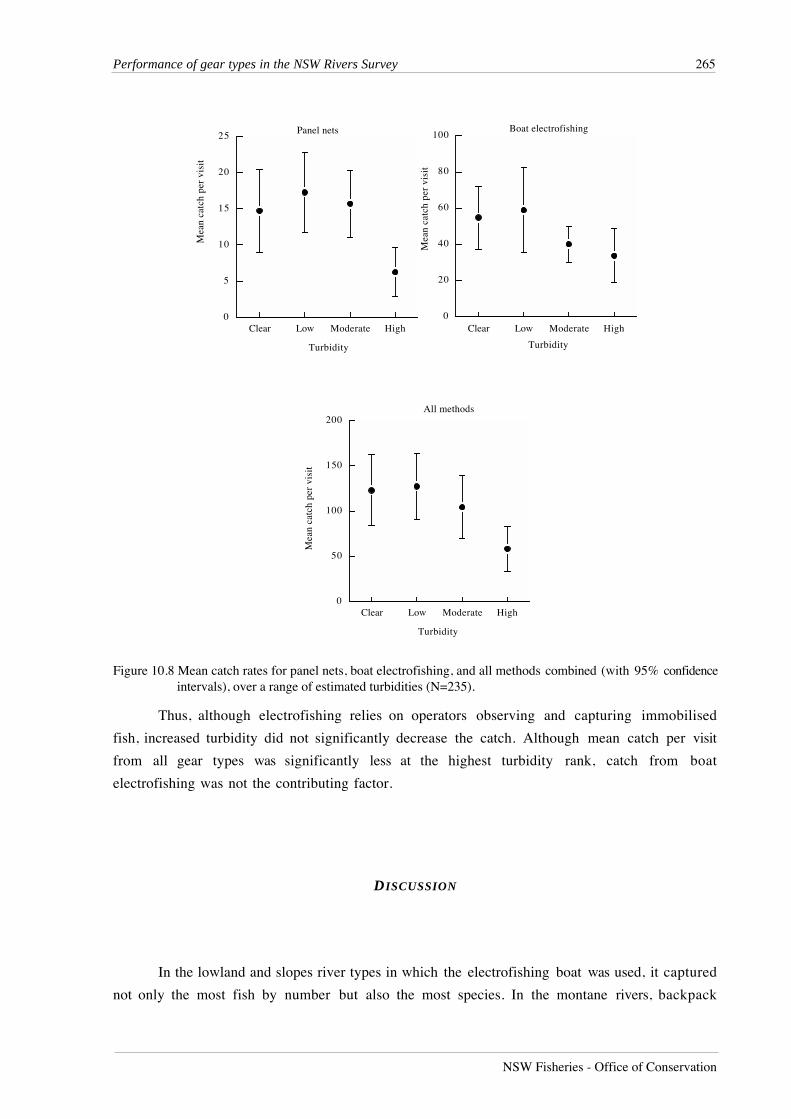
Performance of gear types in the NSW Rivers Survey
NSW Fisheries - Office of Conservation
265
Thus, although electrofishing relies on operators observing and capturing immobilised
fish, increased turbidity did not significantly decrease the catch. Although mean catch per visit
from all gear types was significantly less at the highest turbidity rank, catch from boat
electrofishing was not the contributing factor.
DISCUSSION
In the lowland and slopes river types in which the electrofishing boat was used, it captured
not only the most fish by number but also the most species. In the montane rivers, backpack
0
5
10
15
20
25
Mea
n ca
tch
per
visi
t
Clear Low Moderate High
Turbidity
Panel nets
0
20
40
60
80
100
Mea
n ca
tch
per
visi
t
Clear Low Moderate High
Turbidity
Boat electrofishing
0
50
100
150
200
Mea
n ca
tch
per
visi
t
Clear Low Moderate High
Turbidity
All methods
Figure 10.8 Mean catch rates for panel nets, boat electrofishing, and all methods combined (with 95% confidenceintervals), over a range of estimated turbidities (N=235).
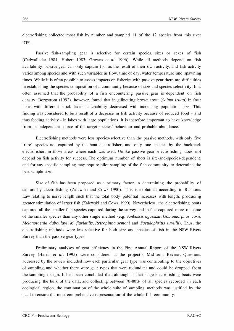
NSW Rivers Survey
CRC For Freshwater Ecology RACAC
266
electrofishing collected most fish by number and sampled 11 of the 12 species from this river
type.
Passive fish-sampling gear is selective for certain species, sizes or sexes of fish
(Cadwallader 1984; Hubert 1983; Growns et al. 1996). While all methods depend on fish
availability, passive gear can only capture fish as the result of their own activity, and fish activity
varies among species and with such variables as flow, time of day, water temperature and spawning
times. While it is often possible to assess impacts on fisheries with passive gear there are difficulties
in establishing the species composition of a community because of size and species selectivity. It is
often assumed that the probability of a fish encountering passive gear is dependent on fish
density. Borgstrom (1992), however, found that in gillnetting brown trout (Salmo trutta) in four
lakes with different stock levels, catchability decreased with increasing population size. This
finding was considered to be a result of a decrease in fish activity because of reduced food - and
thus feeding activity - in lakes with large populations. It is therefore important to have knowledge
from an independent source of the target species’ behaviour and probable abundance.
Electrofishing methods were less species-selective than the passive methods, with only five
‘rare’ species not captured by the boat electrofisher, and only one species by the backpack
electrofisher, in those areas where each was used. Unlike passive gear, electrofishing does not
depend on fish activity for success. The optimum number of shots is site-and-species-dependent,
and for any specific sampling may require pilot sampling of the fish community to determine the
best sample size.
Size of fish has been proposed as a primary factor in determining the probability of
capture by electrofishing (Zalewski and Cowx 1990). This is explained according to Rushtons
Law relating to nerve length such that the total body potential increases with length, producing
greater stimulation of larger fish (Zalewski and Cowx 1990). Nevertheless, the electrofishing boats
captured all the smaller fish species captured during the survey and in fact captured more of some
of the smaller species than any other single method (e.g. Ambassis agassizii, Gobiomorphus coxii,
Melanotaenia duboulayi, M. fluviatilis, Retropinna semoni and Pseudaphritis urvillii). Thus, the
electrofishing methods were less selective for both size and species of fish in the NSW Rivers
Survey than the passive gear types.
Preliminary analyses of gear efficiency in the First Annual Report of the NSW Rivers
Survey (Harris et al. 1995) were considered at the project’s Mid-term Review. Questions
addressed by the review included how each particular gear type was contributing to the objectives
of sampling, and whether there were gear types that were redundant and could be dropped from
the sampling design. It had been concluded that, although at that stage electrofishing boats were
producing the bulk of the data, and collecting between 70-80% of all species recorded in each
ecological region, the continuation of the whole suite of sampling methods was justified by the
need to ensure the most comprehensive representation of the whole fish community.
Performance of gear types in the NSW Rivers Survey
NSW Fisheries - Office of Conservation
267
Growns et al. (1996), in a Hawkesbury River sampling experiment comparing boat
electrofishing and gill nets of mesh sizes ranging from 22 mm to 132 mm, found that the
electrofishing boat captured more species (16) than the mesh nets (7). The electrofishing boat also
captured more fish by number than the nets. They considered that the most effective methods of
collecting fish to discern the effects of a disturbance on community would be those which collect
most species, as the chances of capturing the species which are sensitive to the disturbance is
greater. Faith and Norris (1989) found that for pattern analysis the inclusion of the greatest
number of taxa improves the definition of the environmental gradients. Growns et al. (1996) state
that the use of change in number of indicator species or species richness requires a collecting
method that is unbiased between disturbed and undisturbed sites. Boat electrofishing satisfies these
criteria. Electrofishing also has considerable benefit/cost advantages (Chapter 2): it is rapid, and
can be safely applied by skilled operators in populations of many threatened species or
communities (Cowx and Lamarque 1990, NSW Fisheries, unpublished data). Thus, final results of
the Rivers Survey strongly support the conclusion that electrofishing is the method of choice for
sampling south-east Australian freshwater fish communities.
REFERENCES
Borgstrom, R. (1992). Effect of population density on gillnet catchability in four allopatricpopulations of brown trout (Salmo trutta) Canadian Journal of Fish and Aquatic Sciences49, 1539-45.
Cadwallader. P.L. (1984). Comparison of electrofishing techniques with other collecting methods.First Australian Electrofishing Workshop. Arthur Rylah Institute for EnvironmentalResearch. Technical Report Series No. 17. pp 34-50.
Cowx, I.G. (1990). Developments in Electric Fishing. Fishing News Books, Oxford, UK.
Cowx, I.G. and Lamarque, P. (eds). (1990). Fishing with electricity; applications in freshwaterfisheries management. Fishing News Books, Oxford, UK.
Faith, D.P. and Norris, R.H. (1989). Correlation of environmental variables with patterns ofdistribution and abundance of common and rare freshwater macroinvertebrates.Biological Conservation 50, 77-98.
Growns, I.O., Pollard, D.A, and Harris, J.H. (1996). A comparison of electric fishing andgillnetting to examine the effects of anthropogenic disturbance on riverine fishcommunities. Fisheries Management and Ecology, 3 (1).
Harris, J.H., Bruce, A., Davis, K., Hartley, S., and Silveira, R. (1995). Study of the fish resources ofNSW Rivers. First Annual Report, May 1995, for Natural Resources Audit Council (ProjectG8). NSW Fisheries Research Institute and Cooperative Research Centre for FreshwaterEcology.
Hubert, W.A. (1983). Passive capture techniques. In Nielsen, L.A. and Johnson, D.L. (eds).Fisheries Techniques, American Fisheries Society, Bethesda. pp. 95-122.
Reynolds, J.B. (1983). Electrofishing. In Nielsen, L.A. and Johnson, D.L. (eds). FisheriesTechniques, American Fisheries Society, Bethesda. pp. 147-163.

NSW Rivers Survey
CRC For Freshwater Ecology RACAC
268
Zalewski, M. and Cowx, I.G. (1990). Factors affecting the efficiency of electric fishing. In Cowx,I.G. and Lamarque, P. (eds). (1990) Fishing with electricity; applications in freshwaterfisheries management. Fishing News Books, Oxford, UK.
Acknowledgments 269
CRC For Freshwater Ecology RACAC NSW Fisheries
ACKNOWLEDGMENTS
Many people helped to achieve the successful outcome of the NSW Rivers Survey. Those
who were directly involved in sampling, analysis and reporting are listed below. They included
employed staff of NSW Fisheries at Cronulla and Narrandera, the CRC for Freshwater Ecology
and ACT Parks and Conservation. Seven of those listed were summer students or volunteers from
various universities. The Rivers Survey was completed with support, encouragement, facilities and
funds provided by NSW Fisheries and the Cooperative Research Centre for Freshwater Ecology
(CRCFE), as well as the NSW Resource and Conservation Assessment Council (RACAC) and the
NSW Department of State Development. Helpful comments on a draft of the final report were
provided by NSW Environmental Protection Authority (EPA), NSW Department of Land and
Water Conservation (DLWC) and the Murray-Darling Basin Commission. Professor Peter Cullen
(CRCFE), Dr John Paxton (Australian Museum), Ms Kate Boyd (EPA), Mr Paul O’Connor and Dr
Stuart Rowland (NSW Fisheries), and Mr John Koehn (Marine and Freshwater Research Institute)
all suggested improvements for the report. Comprehensive editing suggestions were provided by
Ms Gillian Higginson (RACAC). A detailed scientific review by Dr Bruce Chessman (DLWC) was
especially valuable. We particularly wish to thank the many landowners who provided access
through their properties to river sites and other support, and who took a close interest in the
progress of the Rivers Survey.
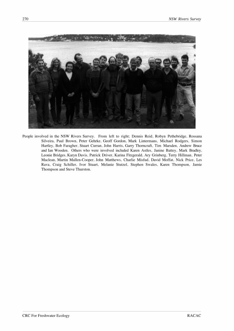
NSW Rivers Survey
CRC For Freshwater Ecology RACAC
270
People involved in the NSW Rivers Survey. From left to right; Dennis Reid, Robyn Pethebridge, RossanaSilveira, Paul Brown, Peter Gehrke, Geoff Gordon, Mark Lintermans, Michael Rodgers, SimonHartley, Bob Faragher, Stuart Curran, John Harris, Garry Thorncraft, Tim Marsden, Andrew Bruceand Ian Wooden. Others who were involved included Karen Astles, Janine Battey, Mark Bradley,Leonie Bridges, Karyn Davis, Patrick Driver, Karina Fitzgerald, Ary Grinberg, Terry Hillman, PeterMaclean, Martin Mallen-Cooper, John Matthews, Charlie Misfud, David Moffat, Nick Price, LesRava, Craig Schiller, Ivor Stuart, Melanie Stutzel, Stephen Swales, Karen Thompson, JamieThompson and Steve Thurston.