draft watershed characterization and model study plan for
TRANSCRIPT
DRAFT
Watershed Characterization and Model Study Plan for the
South Fork Eel River
JULY 7, 2017
PREPARED FOR:
State Water Resources Control Board 1001 I St, Sacramento, CA 95814
PREPARED BY:
Paradigm Environmental 9320 Chesapeake Drive, Suite 100 San Diego, CA 92123

Watershed Characterization and Model Study Plan
THIS PAGE INTENTIONALLY LEFT BLANK

Watershed Characterization and Model Study Plan
June 2017
CONTENTS 1. Introduction............................................................................................................................ 1
1.1 Background ..................................................................................................................... 1 1.2 Study Objectives .............................................................................................................. 2
2. Watershed Characterization .................................................................................................... 3
2.1 Land Characteristics ........................................................................................................ 5 2.2 Climatic Characteristics ................................................................................................... 7 2.3 Geology ........................................................................................................................... 8
Bedrock Geology ...................................................................................................... 8 2.3.1 Surface Processes and Channel Morphology ........................................................... 11 2.3.2 Soils ....................................................................................................................... 11 2.3.3 Hydrogeology ......................................................................................................... 13 2.3.4
2.4 Consumptive Water Use ................................................................................................ 17 Municipal Use ........................................................................................................ 18 2.4.1 Agriculture and Grazing ......................................................................................... 18 2.4.2 Timber Harvest....................................................................................................... 21 2.4.3 Cannabis Cultivation ............................................................................................... 21 2.4.4
2.5 Historic Instream Flows ................................................................................................. 23 3. Model Study Plan ................................................................................................................. 27
3.1 The Model Development Cycle ...................................................................................... 27 3.2 Overview of Proposed Modeling System ........................................................................ 28 3.3 Model Segmentation ...................................................................................................... 29 3.4 Meteorological Boundary Conditions ............................................................................. 33
Primary Precipitation (GHCND) ............................................................................ 34 3.4.1 Secondary Precipitation (PRISM) ........................................................................... 38 3.4.2 Evapotranspiration (CIMIS) ................................................................................... 42 3.4.3
3.5 Other Considerations for Model Configuration .............................................................. 44 Hydrologic Response Units ..................................................................................... 44 3.5.1 Groundwater Interactions ....................................................................................... 45 3.5.2
3.6 Process for Model Calibration and Validation ................................................................ 49 Model Validation.................................................................................................... 57 3.6.1
3.7 Model Scenarios to Investigate Study Objectives ............................................................ 57 4. References ............................................................................................................................ 58
Figures
Figure 2-1. South Fork Eel River watershed. ................................................................................... 4 Figure 2-2. NLCD Land Cover in the South Fork Eel River watershed. .......................................... 6 Figure 2-3. NLCD Percent Impervious Cover in the South Fork Eel River watershed. ..................... 7 Figure 2-4. Geologic map of the South Fork Eel River watershed. ................................................. 10 Figure 2-5. SSURGO Hydrologic Soil Group in the South Fork Eel River watershed. ................... 12 Figure 2-6. Alluvial aquifers recognized within the South Fork Eel River watershed and water provider boundaries. .................................................................................................................... 14 Figure 2-7. Conceptual model for rock moisture and groundwater dynamics in the weathered bedrock zone (Salve et al. 2012). ................................................................................................... 17 Figure 2-8. Grazing pasture and developed areas from the CropScape database April, 2016 ........... 20

Watershed Characterization and Model Study Plan
ii
Figure 2-9. Flow gages in the South Fork Eek River watershed. .................................................... 24 Figure 2-10. Summary of streamflow trends in the South Fork Eel River watershed gages between 1953 and 2014 (adapted from Asarian 2015). ................................................................................ 25 Figure 3-1. Process schematic and example runoff and recharge outputs for the USGS Basin Characterization Model (Flint and Flint 2014). .................................. Error! Bookmark not defined. Figure 3-2. Conceptual schematic of a model development cycle. .................................................. 28 Figure 3-3. Hydrology model schematic (based on Stanford Watershed Model). ............................ 29 Figure 3-4. Elevation and 10-digit hydrologic boundaries of the South Fork Eel River watershed. .. 31 Figure 3-5. Spatial considerations for South Fork Eel River subwatershed delineation ................... 32 Figure 3-6. Historical location of Benbow Lake and Dam. ............................................................ 33 Figure 3-7. Average number of consecutive dry days by month at two South Fork Eel River rainfall stations. ....................................................................................................................................... 35 Figure 3-8. GHCND precipitation gage data before and after patching missing data for the South Fork Eel River watershed. ............................................................................................................ 36 Figure 3-9. PRISM rainfall coverage for the South Fork Eel River watershed vs. selected GHCND gages. ........................................................................................................................................... 39 Figure 3-10. Validation of observed GHCND (047404) vs. PRISM (333015) monthly rainfall totals. .................................................................................................................................................... 40 Figure 3-11. Validation of observed GHCND (048490) vs. PRISM (338636) monthly rainfall totals. .................................................................................................................................................... 41 Figure 3-12. Average monthly reference evaporation for CIMIS zones in the South Fork Eel River watershed. ........................................................................................................................... 43 Figure 3-13. Example summary table showing the intersect of HRU components. ......................... 44 Figure 3-14. Conceptual linkage of a simple groundwater model with HSPF. ................................ 46 Figure 3-15. Currently-available pumping well locations in Mendocino County and the accuracy of these locations. ........................................................................................................................... 48 Figure 3-16. Development of groundwater response functions for HSPF using and a simple groundwater model. ..................................................................................................................... 49 Figure 3-17. Process for model calibration to minimize propagation of uncertainty. ....................... 50 Figure 3-18. Model parameterization and calibration sequence for land hydrology. ....................... 51 Figure 3-19. Model parameterization and calibration sequence for waterbodies and stream transport. .................................................................................................................................................... 51 Figure 3-20. Example calibrated water balance for modeled watershed. ......................................... 53 Figure 3-21. Example surface runoff and evapotranspiration summaries by land use category. ....... 54 Figure 3-22. Examples of daily and monthly modeled versus observed streamflow. ....................... 55 Figure 3-23. Example seasonal average and interquartile modeled versus observed streamflow. ..... 56 Figure 3-24. Process for model validation and identification of data gaps. ..................................... 57 Figure 3-25. Example flow-duration curve analysis to define summer low-flow critical conditions. 58
Watershed Characterization and Model Study Plan
June 2017
Tables
Table 2-1. NLCD land use summary .............................................................................................. 5 Table 2-2. Rainfall summary statistics at the Standish Hickey State Park rainfall gage (048490) ....... 8 Table 2-3. Alluvial aquifers recognized within the South Fork Eel River watershedError! Bookmark not defined. Table 2-4. Water providers and associated water use within the South Fork Eel River watershed. .. 18 Table 2-5. Estimated agricultural water use within the South Fork Eel River watershed. ................ 21 Table 2-6. Summary of USGS streamflow data quantity and quality in the South Fork Eel River watershed ..................................................................................................................................... 26 Table 3-1. Summary of GHCND precipitation gage data before and after patching missing data for the South Fork Eel River watershed .............................................................................................. 37 Table 3-2. Examples of estimated stratification of modeled ET by land cover type ......................... 42 Table 3-3. Performance targets for HSPF hydrology simulation (modeled vs. observed) ................. 52
ACKNOWLEDGEMENTS
The following project team members supported Paradigm Environmental, Inc. in the preparation of this report:
2NDNATURE, LLC GSI Environmental, Inc. R2 Resource Consultants Riverbend Sciences Stillwater Sciences, Inc. S.S. Papadopulos & Associates Daniel Wendell


Watershed Characterization
June 2017
1. INTRODUCTION
1.1 Background
The California Natural Resources Agency, the California Environmental Protection Agency, and the California Department of Food and Agriculture developed the California Water Action Plan (WAP), released on January 22, 2014. The WAP has been developed to meet three (3) broad objectives:
1. More reliable water supplies; 2. The restoration of important species and habitat; and 3. A more resilient, sustainably managed water resources system (water supply, water quality,
flood protection, and environment) that can better withstand inevitable and unforeseen pressures in the coming decades.
Action Four (4) of the WAP, to “Protect and Restore Important Ecosystems,” contains a sub-action that states the following:
“The State Water Resources Control Board and the Department of Fish and Wildlife will implement a suite of individual and coordinated administrative efforts to enhance flows statewide in at least five stream systems that support critical habitat for anadromous fish. These actions include developing defensible, cost-effective, and time-sensitive approaches to establish instream flows using sound science and a transparent public process. When developing and implementing this action, the State Water Resources Control Board and the Department of Fish and Wildlife will consider their public trust responsibility and existing statutory authorities such as maintaining fish in good condition.”
Through a coordinated effort between the State Water Resources Control Board (Water Board) and California Department of Fish and Wildlife (CDFW), the following five (5) priority stream systems have been identified as a starting point for the WAP effort:
1. Shasta River, tributary to the Klamath River, Siskiyou County 2. South Fork Eel River, tributary to the Eel River, Humboldt and Mendocino Counties 3. Mark West Creek, tributary to the Russian River, Sonoma County 4. Mill Creek, tributary to the Sacramento River, Shasta and Tehama Counties 5. Ventura River, Santa Barbara and Ventura Counties
The Water Board and CDFW are currently working to identify potential actions that may be taken to enhance and establish instream flow for anadromous fish in these five (5) priority streams and other streams of importance to the WAP objectives. The development of hydrologic characterization models is one of the first efforts that the Water Board will work on to better understand water supply, water demand, and instream flow needs in the priority watersheds.
This document specifically focuses on the South Fork Eel River (SFER) watershed, and provides:
1. An overview of the characteristics of the watershed that influence hydrology and can inform development of a hydrologic model.
Watershed Characterization and Model Study Plan
2
2. A Study Plan that summarizes the proposed approach to development of a model that meets the study objectives.
1.2 Study Objectives
The objectives of this study and the characteristics of the watershed will influence hydrologic model selection and development. The Water Board identified the following key study objectives to be addressed with the hydrologic model:
Estimation of existing instream flows at multiple points of interest (POI) throughout the mainstem SFER and its tributaries where no flow measurement data are available.
Prediction of unimpaired flows1 at each POI that would occur with no water diversions, pumping, or storage.
Representation of water use and other human activities that impact instream flows and how they affect the water balance.
The model simulation period should be long enough to capture the variability of the full range of water year types from drought to flood years.
In addition, the Water Board identified other model capabilities that should be considered in the current study to support future studies and planning efforts. Although these capabilities may require future model refinements or linkages to other models, the base hydrologic modeling system will be developed in a manner that supports these potential future upgrades or linkages. Additional capabilities of interest include:
Support assessments of habitat for important species. Representation of water rights priority system to evaluate water management scenarios. Projections for climate change and future water demands. Simulation of water quality or the ability to link the surface water hydrology model to
separate water quality models. Simulation of groundwater or the ability to link the surface water hydrology model to a
groundwater model. Section 2 provides a summary of the characteristics of the SFER watershed that influence hydrology and the selection of the modeling approach. Section 3 provides an overview of the Model Study Plan proposed for the project.
1 Unimpaired flow is the flow that would have occurred had the natural flow regime remained unaltered in rivers instead of being stored in reservoirs, imported, exported, or diverted. Unimpaired flow is a modeled flow generally based on historical gage data with factors applied to primarily remove the effects of dams and diversion within the watersheds. Unimpaired flow differs from full natural flow in that the modeled unimpaired flow does not remove changes that have occurred such as channelization and levees, loss of floodplain and wetlands, deforestation, and urbanization. Where no diversion, storage, or consumptive use exists in the watershed, the historical gage data is often assumed to represent unimpaired flow.

Watershed Characterization
June 2017
2. WATERSHED CHARACTERIZATION
The Eel River basin is located in northwestern California, with the Pacific Ocean to the west, Klamath National Forest to the north, and Six Rivers National Forest and Shasta-Trinity National Forest to the east. The Eel River contains approximately 3,526 stream miles, and the main stem (197 miles long) receives flow from 832 perennial tributaries (Eel River Forum 2016). The west side of the watershed is vegetated primarily with redwood and Douglas-fir, while the east side contains mostly grasslands and oak woodlands. Approximately 20% of land is publicly owned by the California State Park system and the U.S. Department of Interior Bureau of Land Management, while the rest is privately owned and primarily used for timber production and cattle and dairy ranching. Less than 100,000 people live in the watershed. The river has been given both state and federal Wild and Scenic River Status (Eel River Forum 2016). Numerous sub-basins and tributaries join the Eel River including the North Fork Eel River (286 square miles), Middle Fork Eel River (753 square miles), which drains the Yolla Bolly Wilderness, Van Duzen River (420 square miles), and the SFER (689 square miles). Located within Mendocino and Humboldt Counties, the SFER watershed is the second largest sub-basin of the Eel River, running northwest from its headwaters near the town of Branscomb to its mouth near the town of Weott (CDFW 2016). Figure 2-1 shows the SFER watershed and subwatersheds defined by the 10-digit Hydrologic Unit Code (HUC) Watershed Boundary Dataset from (WBD) the United States Geological Survey (USGS).
The SFER watershed is known for its high sediment loads, large floods (due to heavy rainfall), and high annual discharge. The SFER has a mean annual discharge of approximately 1.33 million acre-feet as estimated at Miranda (USGS flow gage 11476500) (Eel River Forum 2016). The SFER has a wide range in annual discharge due to the prevailing Mediterranean climate and limited groundwater storage (CDFW 2016). Seasonal weather patterns have a major impact on watershed hydrology, especially during the summer when flows are low and temperatures are high. Rainfall in the winter months is several orders of magnitude higher than during the summer and early fall, which creates higher streamflow rates and water yield (Asarian 2015). In recent years, however, flows have been decreasing due to extended dry periods in winter and early spring, as well as increases in legal and illegal water diversions. There are many surface water diversions and groundwater wells associated with rural residences, cannabis cultivation, pastures, crops, and municipal water systems (Asarian 2015). Since the legalization of cannabis, cultivation of the crop has expanded dramatically in the basin, and is associated with increased water diversions (Bauer et al. 2015). Consumptive water use is discussed in more detail in Section 2.4.
CDFW characterized the Eel River as one of California’s most important anadromous fish streams, ranking second in Coho Salmon and Steelhead Trout production and third in Chinook Salmon production (Eel River Forum 2016). The basin, which once sustained large populations of these species, has seen significant declines in the past century. Much of this decline can be attributed to lost or degraded habitat due to human activities, including commercial and recreational fishing, timber harvest, agricultural practices, water diversions, residential development, and non-native species introduction. In 2005, the California Fish and Game Commission listed Coho Salmon as threatened, and the U.S. Environmental Protection Agency (USEPA) listed all seven sub-basins of the Eel River as impaired on the federal Clean Water Act 303(d) list, primarily for sediment and increased water temperatures.TMDLs have been developed for each sub-basin. Many additional research studies have been performed in the watershed on specific issues or management actions.

Watershed Characterization and Model Study Plan
4
The following sections discuss the SFER watershed in greater detail to provide a full characterization of major factors that influence hydrologic processes. The discussion outlines surface and groundwater resources, geology, land use, climate and precipitation, and soils.
Figure 2-1. South Fork Eel River watershed.

Watershed Characterization
June 2017
2.1 Land Characteristics
In the late 1850s, homesteaders and ranchers began taking possession of land within the SFER watershed and displacing the Sinkyone and Cahto tribes. Due to its remoteness, the watershed did not experience rapid population growth until the 1900s. In the early 1900s, the tanbark industry was the main economic driver in the region, and harvesting tanbark killed many tanoak trees, resulting in deforestation and significant environmental impacts. The industry collapsed around 1920. Timber harvests then increased and had a large impact on the physical nature of the SFER in addition to landscape changes relating to agricultural and ranch land conversion. Highly erosive Franciscan geology is found throughout the watershed, contributing to increased sediment loads in the river. These naturally erosive conditions and high rainfall amounts, combined with the increase in human activities that disturb riparian and upland areas, has led to increased erosion and sedimentation, causing streams to become wider and shallower. Water demand has also increased as residential and urbanized land use continues to rise (NOAA Fisheries 2014).
Land use/land cover data, geology, and soils are the primary GIS layers that form the basis for characterizing surface hydrology. The primary source of land use/land cover for this effort was the 2011 National Land Cover Database (NLCD). Secondary datasets like the CropScape coverage are also available for characterizing vegetative cover for estimating consumptive use, as further described in Section 2.4. Figure 2-2 shows NLCD land use coverage for the SFER watershed. Table 2-1 summarizes the composite land use distribution within the watershed. NLCD also has a grid-based layer that has information on percent impervious cover, shown in Figure 2-3. Detail about geology and soils in the SFER watershed can be found in Section 2.3.1 and Section 2.3.3, respectively.
Table 2-1. NLCD land use summary
NLCD Class Classification Description Area
(acres) Percent
11 Open Water 1,799.68 0.41%
21 Developed, Open Space 18,965.37 4.29%
22 Developed, Low Intensity 790.77 0.18%
23 Developed, Medium Intensity 278.52 0.06%
24 Developed, High Intensity 40.55 0.01%
31 Barren Land 1,467.91 0.33%
41 Deciduous Forest 19,410.55 4.39%
42 Evergreen Forest 296,923.00 67.16%
43 Mixed Forest 18,944.65 4.28%
52 Shrub/Scrub 48,791.43 11.04%
71 Grassland/Herbaceous 33,462.85 7.57%
81 Pasture/Hay 182.93 0.04%
82 Cultivated Crops 64.62 0.01%
90 Woody Wetlands 798.35 0.18%
95 Emergent Herbaceous Wetlands 215.91 0.05%
Total: 442,137.08 100.00%

Watershed Characterization and Model Study Plan
6
Figure 2-2. NLCD Land Cover in the South Fork Eel River watershed.

Watershed Characterization
June 2017
Figure 2-3. NLCD Percent Impervious Cover in the South Fork Eel River watershed.
2.2 Climatic Characteristics
Climate in the SFER watershed is characterized by a long rainy season and a foggy to dry summer season. The rainy season, which generally begins in October and lasts through April, accounts for 90 percent of the mean annual runoff for the Eel River basin. Data from the Standish Hickey State Park rainfall gage, which is centrally-located within the SFER watershed, are representative of typical climate conditions in the watershed. Table 2-2 presents summary statistics of monthly and annual rainfall at this gage. Annual rainfall is about 65 inches at this location, with an annual average of 23 consecutive dry days between storms. The number of consecutive dry days between measurable precipitation from May through October ranges from 19 days to 51 days, but ranges between 9 to 14

Watershed Characterization and Model Study Plan
8
days between November and April. High levels of winter precipitation can lead to widespread flooding throughout the basin (CDFG 2010). Higher rainfalls (i.e. storms ≥0.5 inches per day), which mainly occur during the wettest winter months, have been responsible for shaping the geomorphology of the basin, as further described in Section 2.3. The northern and western regions of the watershed are somewhat influenced by a coastal marine layer, defined by morning fog and overcast conditions, whereas the inland eastern region of the watershed is generally very hot and dry in summer (CDFW 2014). Additional details on the meteorological characteristics and available data to support model development is presented in Section 3.
Table 2-2. Rainfall summary statistics at the Standish Hickey State Park rainfall gage (048490)
Period Mean(in.) Dry
Days High Low 1-Day Maximum Average No. Rain Days1
(in.)
Water Year
(in.) Water Year
(in.) Date ≥0.01 ≥0.10 ≥0.50 ≥1.00
Oct 3.5 33 9.2 1983 0.0 2009 4.8 10/30/1982 6 4 2 1
Nov 8.0 12 23.8 1989 0.0 2004 6.7 11/18/1982 12 8 4 3
Dec 13.1 9 32.0 2003 0.2 1990 10.0 12/14/2002 14 11 7 5
Jan 11.2 9 39.4 1995 0.0 2005 7.0 1/11/2000 14 10 6 4
Feb 10.9 10 33.3 1986 0.0 2010 6.7 2/6/2015 12 10 6 4
Mar 9.3 10 27.3 1983 0.0 1986 4.8 3/13/1983 13 10 6 3
Apr 4.3 14 13.4 1982 0.3 1985 3.5 4/29/2003 9 6 3 1
May 2.6 19 12.2 1990 0.0 2008 3.6 5/22/1990 6 4 2 1
Jun 0.9 27 3.2 2013 0.0 2007 1.8 6/3/1988 3 2 1 0
Jul 0.3 38 2.8 1992 0.0 2014 1.3 7/3/1992 1 0 0 0
Aug 0.3 51 4.7 1983 0.0 2014 3.1 8/31/1983 2 0 0 0
Sep 0.9 46 7.2 1986 0.0 2012 2.4 9/27/1981 2 1 1 0
Annual 65.1 23 132.4 1983 33.8 2008 10.0 12/14/2002 95 67 39 23
1: Average number of rainfall days with a rainfall total greater than or equal to the depth (inches) shown. 2: Relative Color Gradient: Rainfall depth/distribution and average consecutive dry days. Darker is higher.
2.3 Geology
Bedrock Geology 2.3.1The SFER watershed can be divided into three general planning sub-basins (Northern, Eastern, and Western) (Figure 3-4) that are based largely on bedrock geology, hydrologic and surficial geomorphic processes, and land cover characteristics (CDFW 2014). Differences in the composition and strength of bedrock firmly control variability in topography, drainage network, surficial geomorphic processes, and hydrology between the sub-basins.
The Eel River watershed is in a tectonically active plate-boundary deformation zone, defined by right-lateral movement along the San Andreas Fault Zone that separates the Pacific plate to the west from the North American plate to the east (Kelsey and Carver 1988). Northward progression of the San Andreas Fault Zone is characterized by lateral shearing and vertical compression due to the major westward turn in the fault zone upon reaching the Mendocino Triple Junction near Cape Mendocino. These primary deformation styles are what create the dominant NNW-SSE trending

Watershed Characterization
June 2017
topographic and structural grain in the region. The evolution of this regional topographic and structural grain has developed pervasive shearing, fracturing, and faulting throughout the north coast of California. These geologic structures have significant implications for where groundwater is stored and how it is transmitted through the landscape.
The SFER watershed is predominantly composed of the Franciscan Complex, consisting of three structurally separated belts: the Eastern, Central, and Coastal belts (Figure 2-4) (Jayko et al. 1989). These belts decrease in age from east to west, reflecting accretion of oceanic sediments to western North America. The western portion of the watershed is predominantly underlain by the Coastal and Yager Terranes of the Coastal Belt Franciscan Complex. The Coastal Terrane and Yager Terrane consist predominantly of fine-grained marine sandstone, argillite, and minor conglomerate. The higher rock-strength in Coastal Belt rocks in the western side of the basin typically leads to steeper, ridge-and-valley topography with better organized drainage networks compared to the eastern side. The eastern side of the watershed is predominantly underlain by the Central Belt Franciscan Complex. The Central belt consists of a Late Jurassic to Middle Cretaceous argillaceous mélange matrix encompassing blocks and slabs of sandstone and shale turbidite sequences (McLaughlin et al. 2000). The Central belt is especially prone to widespread landsliding in the form of large earthflow complexes (Brown and Ritter 1971, Mackey and Roering 2011), typically leading to hummocky topography with disorganized drainage networks. Large blocks of meta-sandstone, meta-basalt and high-grade blueschist rocks occur as topographic highs within the Central belt.
Overlying the accreted Franciscan Complex belts are deposits of younger marine sedimentary rocks, as well as river terraces, alluvial valley fills, alluvial fans, and landslide deposits (McLaughlin et al. 2000). Landslides and geomorphic features related to landsliding have been mapped from aerial photography throughout most of the SFER watershed (CDMG 1999). Alluvial valley fills are unconsolidated to loosely cemented gravel, sand, silt, and clay deposited in the major valleys and small basins along major stream courses during the Quaternary Period. The larger alluvial valley fills (e.g. Leggett area and Laytonville Valley) were deposited in topographically separated structural basins. Consequently, the units are correlative from one basin to another but are not continuous between basins. Farrar (1986) subdivided valley fill into three hydrogeologic units based on age and origin: continental basin deposits, continental terrace deposits, and Holocene alluvium. The geologic attributes of each unit result in differences in water-bearing properties.

Watershed Characterization and Model Study Plan
10
Figure 2-4. Geologic map of the South Fork Eel River watershed.

Watershed Characterization and Model Study Plan
June 2017
Surface Processes and Channel Morphology 2.3.2The Eel River has the highest recorded average suspended sediment load per unit area of any river of its size or larger in the conterminous United States (Lisle 1990). The high erosion and sediment transport rates have been attributed to a combination of rapid uplift and tectonic deformation, erosive bedrock, high seasonal rainfall and intense storm events, and anthropogenic disturbance (e.g. forest management, road construction, and agriculture). The SFER watershed has proportionally less sediment supply and transport than other Eel River sub-basins (USEPA 1999). Stream channel morphology and grain size in the Eel River basin is closely linked to stochastic hillslope processes and high flow events that produce and transport fluvial sediment (Lisle 1982).
Historical land use changes (e.g. timber harvest and associated vegetation change, road development, increased impervious surface area, and water diversions) and large flood events have increased channel sediment storage, simplified channel morphology, and altered basin hydrologic responses (e.g. more rapid runoff, less groundwater retention, and reduced dry-season streamflow). Some reaches of the mainstem SFER aggraded up to 11 feet from 1968 to 1998 (USACE 1999). Notable sedimentation has also occurred in SFER tributaries. Cuneo Creek, for example, aggraded more than 30 feet and widened from 30 to 300 feet (LaVen 1987; Short 1987). Channels in the watershed typically recover from large events over decades of subsequent exposure to smaller discharges that remobilize and sort stored sediment (Lisle 1981; Lisle 1982). In some reaches, channel patterns and flood deposits along the higher channel margins may persist until floods of equal or greater magnitude occur (Kelsey 1977; Lisle 1981).
Major knickzones in the SFER watershed reflect channel incision in response to regional uplift and base-level lowering. A prominent eight-mile long, 380-foot tall knickzone has developed on the mainstem of the SFER between Rattlesnake Creek (RM 74) and Tenmile Creek (RM 82) (CDFW 2014). Associated tributary knickzones are expressed as waterfalls or cascade channel reach morphology (Foster 2010). Minor knickzones can form in response to variable rock resistance, faulting, and base level control induced by landslide deposits.
Soils 2.3.3Weak bedrock in the SFER watershed results in a moderate to highly unstable soil mantle prone to erosion and transport by mass wasting, fluvial processes, and wind. Predominantly silt-loam to cobbly-loam soil types range from 1 to 7 feet in depth. The dominant soil series in the SFER watershed is Wohly-Holohan-Casabonne which covers approximately 43% of the basin area (CDFW 2014) and is associated with mélange and sandstone bedrock of the Central Belt, Coastal Belt, and Yager Terrane (CDFW 2014).
The State Soil Geographic and Soil Survey Geographic Database (STATSGO/SSURGO) has four main hydrologic soil groups that characterize soil runoff potential. Group A generally has the lowest runoff potential and Group D has the highest runoff potential. The soils database is composed of a GIS layer of polygon map units, and a linked database with multiple soil properly tables. Figure 2-5 presents the spatial distribution and a tabular summary of the STATSGO/SSURGO hydrologic soil groups for the SFER watershed. The dominant soil group in the watershed is Group B, containing moderately well to well-drained silt loams and loams. Group C is the next most common soil group in the watershed, containing sandy clay loam that typically have low infiltration rates.

Watershed Characterization and Model Study Plan
12
Figure 2-5. SSURGO Hydrologic Soil Group in the South Fork Eel River watershed.

Watershed Characterization and Model Study Plan
June 2017
Hydrogeology 2.3.4
Alluvial Aquifers 2.3.4.1
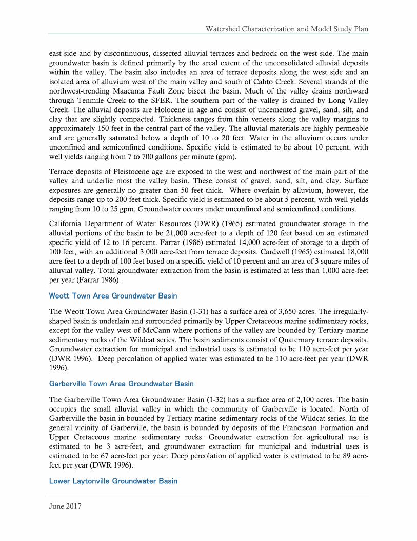
There are five major alluvial aquifers within the SFER watershed (Table 2-3, Figure 2-6). These alluvial aquifers consist of primarily sand and gravel and finer sediments within Holocene alluvium and older Quaternary terraces (Farrar 1986). Holocene alluvial deposits are uncemented and only slightly compacted, whereas Quaternary terraces have varying degrees of cementation and compaction that typically increase with age. Porosity and permeability in these alluvial aquifers is generally high. The larger alluvial valley fills occur in the Laytonville Valley and Leggett area. Groundwater contours in these areas are approximately concentric with the outline of the valley floor, indicating that groundwater moves from the valley margins toward the center (Farrar 1986). Quaternary river terraces occur throughout the mainstem SFER valley and larger tributary valleys.
Table 2-3. Alluvial aquifers recognized within the South Fork Eel River watershed
Basin Name Area (acres) Groundwater
Budget Type1
1-12 Laytonville Valley 5,020 A
1-31 Weott Town Area 3,650 B
1-32 Garberville Town Area 2,100 B
1-38 Lower Laytonville Valley 2,150 C
1-39 Branscomb Town Area 1,320 C
1 (A) a groundwater budget exists, a groundwater model exists that can be used to calculate a groundwater budget, or groundwater extraction data exist; (B) use-based estimate of groundwater extraction for the basin; (C) not enough data exists to provide an estimate of the groundwater budget (DWR 1996).

Watershed Characterization and Model Study Plan
14
Figure 2-6. Alluvial aquifers recognized within the South Fork Eel River watershed and water provider boundaries.
Laytonville Valley Groundwater Basin
The Laytonville Valley Groundwater Basin (1-12) has a surface area of 5,020 acres. The valley consists of a narrow alluvium-filled trough bounded by bedrock of the Franciscan Complex on the
Watershed Characterization and Model Study Plan
June 2017
east side and by discontinuous, dissected alluvial terraces and bedrock on the west side. The main groundwater basin is defined primarily by the areal extent of the unconsolidated alluvial deposits within the valley. The basin also includes an area of terrace deposits along the west side and an isolated area of alluvium west of the main valley and south of Cahto Creek. Several strands of the northwest-trending Maacama Fault Zone bisect the basin. Much of the valley drains northward through Tenmile Creek to the SFER. The southern part of the valley is drained by Long Valley Creek. The alluvial deposits are Holocene in age and consist of uncemented gravel, sand, silt, and clay that are slightly compacted. Thickness ranges from thin veneers along the valley margins to approximately 150 feet in the central part of the valley. The alluvial materials are highly permeable and are generally saturated below a depth of 10 to 20 feet. Water in the alluvium occurs under unconfined and semiconfined conditions. Specific yield is estimated to be about 10 percent, with well yields ranging from 7 to 700 gallons per minute (gpm).
Terrace deposits of Pleistocene age are exposed to the west and northwest of the main part of the valley and underlie most the valley basin. These consist of gravel, sand, silt, and clay. Surface exposures are generally no greater than 50 feet thick. Where overlain by alluvium, however, the deposits range up to 200 feet thick. Specific yield is estimated to be about 5 percent, with well yields ranging from 10 to 25 gpm. Groundwater occurs under unconfined and semiconfined conditions.
California Department of Water Resources (DWR) (1965) estimated groundwater storage in the alluvial portions of the basin to be 21,000 acre-feet to a depth of 120 feet based on an estimated specific yield of 12 to 16 percent. Farrar (1986) estimated 14,000 acre-feet of storage to a depth of 100 feet, with an additional 3,000 acre-feet from terrace deposits. Cardwell (1965) estimated 18,000 acre-feet to a depth of 100 feet based on a specific yield of 10 percent and an area of 3 square miles of alluvial valley. Total groundwater extraction from the basin is estimated at less than 1,000 acre-feet per year (Farrar 1986).
Weott Town Area Groundwater Basin
The Weott Town Area Groundwater Basin (1-31) has a surface area of 3,650 acres. The irregularly-shaped basin is underlain and surrounded primarily by Upper Cretaceous marine sedimentary rocks, except for the valley west of McCann where portions of the valley are bounded by Tertiary marine sedimentary rocks of the Wildcat series. The basin sediments consist of Quaternary terrace deposits. Groundwater extraction for municipal and industrial uses is estimated to be 110 acre-feet per year (DWR 1996). Deep percolation of applied water was estimated to be 110 acre-feet per year (DWR 1996).
Garberville Town Area Groundwater Basin
The Garberville Town Area Groundwater Basin (1-32) has a surface area of 2,100 acres. The basin occupies the small alluvial valley in which the community of Garberville is located. North of Garberville the basin in bounded by Tertiary marine sedimentary rocks of the Wildcat series. In the general vicinity of Garberville, the basin is bounded by deposits of the Franciscan Formation and Upper Cretaceous marine sedimentary rocks. Groundwater extraction for agricultural use is estimated to be 3 acre-feet, and groundwater extraction for municipal and industrial uses is estimated to be 67 acre-feet per year. Deep percolation of applied water is estimated to be 89 acre-feet per year (DWR 1996).
Lower Laytonville Groundwater Basin

Watershed Characterization and Model Study Plan
16
The Lower Laytonville Groundwater Basin (1-38) has a surface area of 2,150 acres. Lower Laytonville Valley is a narrow north and northwest-trending alluvial basin. The town of Laytonville is situated approximately 1.5 miles southeast of the southern extent of this valley. The main alluvial portion of the valley is approximately 4 miles long and ranges in width from 0.25 to 1 mile. The groundwater basin is primarily defined by the areal extent of unconsolidated alluvial deposits within the valley bounded by Franciscan Complex. Terrace deposits located northeast and west of the main alluvial valley are also included in the basin. This basin is separated from the Laytonville Valley Groundwater Basin to the south by a narrow section of Tenmile Creek formed in Franciscan Complex bedrock. Strands of the northwest-trending Maacama Fault Zone bisect the basin. Water bearing formations in Lower Laytonville Valley include Holocene alluvium and older terrace deposits of Pliocene to Pleistocene age. Based on information from wells installed in Holocene alluvium in Laytonville Valley, yields in this formation range from 7 to 700 gpm and estimated specific yields range from 10 to 16 percent (DWR 1965). Based on information from wells installed in older terraces deposits in Laytonville Valley, water yields range from 10 to 25 gpm and estimated specific yields are 5 percent (DWR 1996).
Branscomb Town Area Groundwater Basin
The Branscomb Town Area Groundwater Basin (1-38) has a surface area of 1,320 acres. This elongate, north and northwest-trending valley is about 6 miles in length and has a width ranging from about 0.2 to 0.7 miles. The Branscomb Town Area Groundwater Basin is defined by the areal extent of Holocene and Quaternary Alluvium, which is bounded on all sides by bedrock of the Franciscan Formation. Alluvium and river channel deposits of Holocene age consist largely of unconsolidated silts, gravels, clays, and sands. Limited data suggests the alluvium averages 10 to 15 feet thick (DWR 1958). The maximum thickness of these deposits is unknown. No published well yield or specific yield data were identified for wells in this area; however, wells drilled in small nearby alluvial valleys have been unproductive due to low permeability. Groundwater in the alluvial deposits is typically unconfined but may be locally semi-confined.
Fractured-Rock Aquifers 2.3.4.2
Most the SFER watershed is underlain by fractured-rock aquifers that occur in the mountainous areas. Water movement from hillslopes to stream channels in fractured-rock aquifers is controlled by topography, bedrock lithology, stratigraphic structure (e.g. bedding planes contained within sedimentary units of the Coastal belt Franciscan Complex), structural deformation (e.g. fracturing and internal shear), and the properties of weathering rock. The increased hydraulic conductivity and porosity in weathered bedrock allows water to perch on underlying fresh bedrock and flow laterally to stream channels. The depth and topography of weathered bedrock is therefore an important factor influencing runoff (Rempe and Dietrich 2014). Where hillslopes are composed of a soil mantle and weathered bedrock zone over fresh bedrock (e.g. western portion of the SFER watershed), runoff occurs as overland flow, shallow subsurface flow perched at the soil-bedrock boundary, and flow through fractured or fresh bedrock (Salve et al. 2012) (Figure 2-7). Perched groundwater can deliver most of the stream runoff and can be the source of sustained summer baseflow (Salve et al. 2012). Deep runoff can also be generated on hillslopes during storms if precipitation moves quickly through the weathered unsaturated zone (Salve et al. 2012). In-field studies of soil and rock moisture dynamics in a western SFER sub-basin, Salve et al. (2012) found: (1) the first rains after a dry season rapidly penetrate through the soil mantle and into the underlying weathered bedrock; (2) large rains generate a response as deep as 20 feet into the weathered bedrock within a few weeks, but the

Watershed Characterization and Model Study Plan
June 2017
perched groundwater responds within hours to days of the start of rain; (3) rock moisture in the shallow, weathered bedrock tends to vary less after initial wet up; and (4) water transmitted to the water table through fracture flow is a key process influencing runoff characteristics. Groundwater from fractured-rock aquifers tends to supply individual domestic and stock wells, or small community water systems and tends to have less capacity and reliability than wells in alluvial aquifers.
Figure 2-7. Conceptual model for rock moisture and groundwater dynamics in the weathered bedrock zone (Salve et al. 2012).
2.4 Consumptive Water Use
Since the establishment of residences and smaller ranches during the last century, the need for water supplies in the SFER watershed has increased, with most of the current demand satisfied by in-stream diversions or shallow wells (NOAA Fisheries 2014). For the entire Eel River basin, most usable water is delivered during the winter months with only 1.5% of the annual flow occurring during the 5 driest months of the year (June – October) (Eel River Forum 2016). Water is extracted throughout the basin for domestic, agricultural (including Cannabis), municipal, stock watering, fish culture, fire protection, and road dust control (primarily for timber harvest) purposes.
Watershed Characterization and Model Study Plan
18
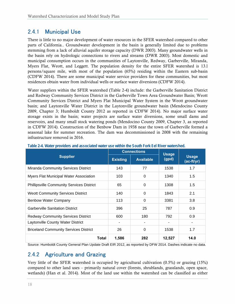
Municipal Use 2.4.1There is little to no major development of water resources in the SFER watershed compared to other parts of California.. Groundwater development in the basin is generally limited due to problems stemming from a lack of alluvial aquifer storage capacity (DWR 2003). Many groundwater wells in the basin rely on hydrologic connections to rivers and streams (DWR 2003). Most domestic and municipal consumption occurs in the communities of Laytonville, Redway, Garberville, Miranda, Myers Flat, Weott, and Leggett. The population density for the entire SFER watershed is 13.l persons/square mile, with most of the population (65%) residing within the Eastern sub-basin (CDFW 2014). There are some municipal water service providers for these communities, but most residences obtain water from individual wells or surface water diversions (CDFW 2014).
Water suppliers within the SFER watershed (Table 2-4) include: the Garberville Sanitation District and Redway Community Services District in the Garberville Town Area Groundwater Basin; Weott Community Services District and Myers Flat Municipal Water System in the Weott groundwater basin; and Laytonville Water District in the Laytonville groundwater basin (Mendocino County 2009, Chapter 3; Humboldt County 2012 as reported in CDFW 2014). No major surface water storage exists in the basin; water projects are surface water diversions, some small dams and reservoirs, and many small stock watering ponds (Mendocino County 2009, Chapter 3, as reported in CDFW 2014). Construction of the Benbow Dam in 1938 near the town of Garberville formed a seasonal lake for summer recreation. The dam was decommissioned in 2008 with the remaining infrastructure removed in 2016.
Table 2-4. Water providers and associated water use within the South Fork Eel River watershed.
Supplier Connections
Usage (gpd)
Usage
(ac-ft/yr) Existing Available
Miranda Community Services District 143 77 1538 1.7
Myers Flat Municipal Water Association 103 0 1340 1.5
Phillipsville Community Services District 65 0 1308 1.5
Weott Community Services District 140 0 1843 2.1
Benbow Water Company 113 0 3381 3.8
Garberville Sanitation District 396 25 787 0.9
Redway Community Services District 600 180 792 0.9
Laytonville County Water District - - - -
Briceland Community Services District 26 0 1538 1.7
Total 1,586 282 12,527 14.0
Source: Humboldt County General Plan Update Draft EIR 2012, as reported by DFW 2014. Dashes indicate no data.
Agriculture and Grazing 2.4.2Very little of the SFER watershed is occupied by agricultural cultivation (0.5%) or grazing (15%) compared to other land uses – primarily natural cover (forests, shrublands, grasslands, open space, wetlands) (Han et al. 2014). Most of the land use within the watershed can be classified as either

Watershed Characterization and Model Study Plan
June 2017
timber harvest, or open space and parks. Approximately 20% of land ownership in the watershed is publicly owned by the California State Park system, the U.S. Department of Interior, Bureau of Land Management, and large timber companies. Ranches, small communities, and rural residential areas make up most of the remaining lands (CDFW 2016).
DWR provides the best data available for estimating crop-specific water application and consumptive use rates, and the SFER watershed matches DWR’s most detailed geographic scale of data, a ‘detailed analysis unit.’ The U.S. Department of Agriculture (USDA) CropScape dataset provides spatial files that depict coverage of a wide array of crop types across the U.S. at the 30-meter pixel scale, and a minimum mapping unit of 1 pixel (approximately 0.25 acre) (Han et al. 2014). Land use from the CropScape database was classified into categories that align with the DWR irrigated crops data to illustrate areal coverage of irrigated and developed areas. DWR data were used to estimate agricultural consumptive use across the watershed (see Figure 2-8).

Watershed Characterization and Model Study Plan
20
Figure 2-8. Grazing pasture and developed areas from the CropScape database April, 20162
2 https://nassgeodata.gmu.edu/CropScape/ (Han et al. 2014). Note that agricultural crops are present in the basin, but occupy too small an area to show on the map.

Watershed Characterization and Model Study Plan
June 2017
Land use from the CropScape database was classified into categories that align with the DWR irrigated crops data to estimate agricultural consumptive uses across the watershed. Water usage data were available for 2005-2010 from DWR for the SFER watershed. Most of the watershed includes natural cover (forests, shrublands, grasslands, open space, wetlands) with only small portions attributed to urban development, grazing pastures, or agricultural cultivation (Table 2-5). Grazing pastures are the most prevalent land use identified in the CropScape data with associated water use data from DWR, but only a small portion of this area is listed as irrigated area during any single year by DWR (Table 2-5) compared to the area mapped in the CropScape data. Other deciduous crops (identified as Pears in the CropScape data), row crops, and vineyards make up the remainder of cultivated area. A few other crop types are present in the watershed, but with very small acreages and no corresponding irrigated acreage listed by DWR (see Table 2-5). Based on these data, the total annual consumptive use from agricultural crop and grazing pastures is approximately 209.8 acre-feet/year.
Table 2-5. Estimated agricultural water use within the South Fork Eel River watershed.
Crop Types
Irrigated Area (ac) (DWR)
Consumptive Use
(ac-ft/ac/year)
Consumptive Use
(ac-ft/year) USDA CropScape DWR
Grass/Pasture Pasture 69.77 2.47 172.3
Clover/Wildflowers
Pears Other Deciduous
0.38 1.45 0.6
Fallow/Idle Cropland Row Crops 20.84 0.70 14.6
Grapes Vineyards 62.07 0.36 22.3
Total 153.06 209.8
Crop types are listed for both USDA CropScape data and DWR along with irrigated acreage from DWR and water usage for each CWDR crop type. Vineyards, Grain, Pistachios, Corn, and Alfalfa crop types occurred in the CropScape data, but there were no corresponding water use estimates from DWR.
Timber Harvest 2.4.3Water is used for dust abatement on timber company roads throughout Humboldt and Mendocino Counties between May 15th
and October 15th (CDFW 2014). Estimates of water used each harvest season range from 2,000 to 4,000 gallons/mile/day (treating two times each day). One timber company with approximately 400,000 acres located in Northwestern California estimated an annual use of two million gallons for dust abatement (CDFW 2014). Given the anecdotal nature of these accounts and limited information sources, a reliable overall estimate of consumptive water use from timber harvest is not currently feasible for the entire SFER watershed.
Cannabis Cultivation 2.4.4Mendocino and Humboldt Counties are home to some of the largest Cannabis growing operations in California, which have been increasing in number and scale during recent years. The consumptive demand for Cannabis farms impact summer stream flows during low-flow periods. This altered hydrologic function is one of the most critical stressors for juvenile salmonids in the SFER

Watershed Characterization and Model Study Plan
22
watershed, particularly in more urbanized areas such as the Salmon Creek and Redwood Creek watersheds where Cannabis cultivation coincides with domestic usage (NOAA Fisheries 2014).
Cannabis growing has not been comprehensively mapped for the entire SFER watershed, but recent studies that identify grow operations via aerial imagery provide some key insights on consumptive water use in many watersheds. A CDFW study by Bauer et al. (2015) identified 567 grows (estimated 20,000 plants) in the Salmon Creek drainage and 549 grows (estimated 18,000 plants) in the Redwood Creek watershed. These operations were estimated to consume more than 55.2 and 50.6 acre-feet of water per season in Salmon Creek and Redwood Creek, respectively (Bauer et al. 2015). In 60 randomly sampled 12-digit subwatersheds in Humboldt County with an average size of 109 km2, Butsic and Brenner (2016) counted an average of 70 grows and 4770 plants per subwatershed, equating to an estimated water use of 9 acre-feet per sub-watershed. Butsic and Brener (2016) noted that the number and size of Cannabis sites has likely continued to increase since their analysis. In the Mad River watershed, north of the SFER, Bauer (2015) found that the acreage under cultivation increased approximately 170% from 2009 to 2014, equivalent to 34% per year. Butsic and Brener (2016) and Bauer et al. (2015) both use Humboldt Growers Association (2010) estimates of 22.7 liters per plant per day and a 150-day growing season to estimate per-plant water usage as 3,405 liters (0.0028 acre-feet) per year. Bauer et al. (2015) estimated a range of 76 – 132 plants/km2
within the study watersheds, and Butsic and Brenner (2016) calculated an average of 4,770 plants per each similarly sized subwatershed. Given the SFER watershed has an approximate area of 1782 km2, Bauer’s estimates of plant density would provide a range between 135,000 – 235,000 plants for the entire watershed. With 19 subwatersheds within the SFER watershed on the same order as Butsic and Brenner’s sample (WBD 12-digit HUC), their mean plant number would provide an estimate of 90,630 plants within the SFER watershed. Since Bauer et al. (2015) selected watersheds with known high densities of Cannabis cultivation, it is not surprising that the estimate is higher than the random sample of Butsic and Brenner (2016), which is probably a more appropriate number for inference about the entire SFER watershed in the absence of other information. Given the mean number of plants (4,770) calculated by Butsic and Brener (2016), water use for Cannabis cultivation within the entire SFER watershed can be roughly estimated at 252 acre-feet/yr.
Upon request Butsic ran a GIS intersection of plant counts and four land ownership categories (public, tribal, timber company, and other private), and provided a county-wide summaries (not watershed level summaries due to privacy concerns) for those land ownership categories. The results indicate a much higher density of plants on "other private" land (70 plants/km2), whereas the other categories ranged from 0.3-2 plants/km2 (Van Butsic, personal comm., October 13, 2016). These densities could be combined with a land ownership GIS layer to generate a spatially specific estimate for use in hydrologic modeling.
With the clandestine nature of Cannabis cultivation, data are limited and likely have a high degree of uncertainty in both plant water usage estimates as well as number of grow sites and plants within the SFER watershed. However, given the high degree of impacts on summer low flows, capturing this component of consumptive use within the basin will be important. Additional information about observed plant density for specific subwatersheds would be valuable to incorporate into future estimates and constrain uncertainty in water usage estimates.

Watershed Characterization and Model Study Plan
June 2017
2.5 Historic Instream Flows
There are five USGS streamflow gages in the SFER watershed with observed data between water years 2007 and 2016. There are three other gages that have observed data between 1957 and 2006. The data were analyzed to assess the quantity and quality of the observed record. Table 2-6 is a summary of USGS data quantity and quality in the SFER watershed. Additional recent flow data are available from CalTrout gages (2015-2016) in Sproul Creek, Salmonid Restoration Federation (SRF) gages (2015) in Redwood Creek (Klein and Eastwood 2016), and the University of California, Berkeley gage (1990 to present) at historic (1947-1970) USGS gage 11475500. Gage locations in the SFER watershed are shown in Figure 2-9Error! Reference source not found.. The Water Board is in the process of installing multiple additional flow gages in the watershed that will be active in 2017. During model development, streamflow data from all available sources will be further assessed to identify important critical conditions in space and time to focus on during model calibration. Data quantity and quality will impact both the selection of data to be used for calibration as well as the interpretation of model performance during those associated time periods. More weight will be given to locations and time periods with higher quantity and quality of data.
Previous studies have analyzed streamflow trends in the SFER watershed. For example, Asarian (2015) found statistically-significant declining streamflow trends at most tributary sites of the Eel River basin (during the summer low-flow season) between 1953 and 2014 (Figure 2-10). The streamflow declines were most pronounced from July through mid-October. In addition to looking at streamflow, the study also examined precipitation-adjusted streamflow, which statistically reduces fluctuations caused by precipitation variability that occurs from year to year. The results suggest that precipitation can explain only a portion of the streamflow declines. For example, Elder Creek, a tributary to the SFER, is one of the most undisturbed watersheds within the SFER basin. Elder Creek experienced a declining trend in streamflow but showed very little change in precipitation-adjusted streamflow. This suggests that a portion of the streamflow decrease at the other gages may be attributed to other factors such as increased diversions or increased evapotranspiration due to changes in vegetation composition (e.g. due to fire suppression or timber harvest) or climate (e.g. increased air temperature or reduced fog). Because evapotranspiration comprises a major component of the water budget, even small changes in evapotranspiration may have an amplified effect on summer streamflows.
Other studies have attributed the decline of endangered species of anadromous fish, such as the coho salmon, to the decline in summer streamflows (NMFS 2014; Bauer et al. 2015). While water diversions were not quantified by Asarian (2015), the results of the precipitation-adjusted streamflow analysis suggest that diversions are a significant contributing factor to declining summertime flows and, thus, anadromous fish habitat. CDFW estimates of diversions related to cannabis cultivation range from 1 to 10 cubic meters per day per square kilometer of watershed area (Bauer 2015; Bauer et al. 2015), while Asarian (2015) found that the magnitude of decline in precipitation-adjusted streamflow at gages within the SFER was 30 to 100 cubic meters per day per square kilometer of watershed area. If those estimates are correct, it suggests that cannabis cultivation may account for approximately 1 to 33 percent of the total precipitation-adjusted streamflow declines experienced in the Eel River basin. The remaining decline might be attributed to other factors that increase evapotranspiration, as discussed in the preceding paragraph.

Watershed Characterization and Model Study Plan
24
Figure 2-9. Flow gages in the South Fork Eek River watershed.3
3 Map does not include locations of flow gages currently being installed by the Water Board.

Watershed Characterization and Model Study Plan
June 2017
Figure 2-10. Summary of streamflow trends in the South Fork Eel River watershed gages between 1953 and 2014 (adapted from Asarian 2015).4
4 Number of days in May through October (184 possible days) with increasing or decreasing trends in (A) streamflow and (B) precipitation-adjusted streamflow at mainstem and tributary sites for WY 1953 – 2014. Bars are stacked with colors indicating statistical significance and labels indicating the total number of days with an increasing or decreasing trend. Summary of WY1953-2014 Mann-Kendall trend tests for each (365) day of the year for (A) streamflow and (B) precipitation-adjusted streamflow at long-term USGS gages in the SFER watershed. Symbols are color-coded by direction and statistical significance of the trend. Dashed lines are LOESS (Locally Estimated Scatterplot Smoothing) curves provided as visual aids to indicate the overall seasonal pattern. A horizontal line is placed at zero in each panel, so declining days are below the line and increasing days are above the line. Average (mean) of all July-October days is shown in lower-left corner of each panel.

Watershed Characterization and Model Study Plan
26
Table 2-6. Summary of USGS streamflow data quantity and quality in the South Fork Eel River watershed
1957
1958
1959
1960
1961
1962
1963
1964
1965
1966
1967
1968
1969
1970
1971
1972
1973
1974
1975
1976
11475500 ● ● ● ● ● ● ● ● ● ● ● ● ● ●
11475560 ● ● ● ● ● ● ● ● ●
11475610
11475700 ● ● ● ● ● ● ● ● ● ● ● ● ● ● ● ● ●
11475800 ● ● ● ● ● ● ● ● ● ● ●
11475940 ● ● ● ● ● ● ●
11476500 ● ● ● ● ● ● ● ● ● ● ● ● ● ● ● ● ● ● ● ●
11476600 ● ● ● ● ● ● ● ● ● ● ● ● ● ● ● ●
1977
1978
1979
1980
1981
1982
1983
1984
1985
1986
1987
1988
1989
1990
1991
1992
1993
1994
1995
1996
11475500
11475560 ● ● ● ● ● ● ● ● ● ● ● ● ● ● ● ● ● ◕ ● ●
11475610
11475700
11475800 ● ● ● ● ● ● ● ● ● ● ● ● ● ● ● ● ● ● ●
11475940
11476500 ● ● ● ● ● ● ● ● ● ● ● ● ● ● ● ● ● ● ● ●
11476600 ● ● ● ● ● ● ● ● ● ● ● ● ◕ ● ◕ ◕ ● ● ◕ ◕
1997
1998
1999
2000
2001
2002
2003
2004
2005
2006
2007
2008
2009
2010
2011
2012
2013
2014
2015
2016
11475500
11475560 ● ● ● ● ● ● ● ● ● ● ● ● ● ● ● ● ● ● ● ●11475610 ● ● ● ● ● ● ● ● ●11475700
11475800 ● ● ● ● ● ● ● ● ◕ ● ● ● ● ● ● ● ●
11475940
11476500 ● ● ● ● ● ● ● ● ● ● ● ● ● ● ● ● ● ● ● ◕
11476600 ● ◕ ● ● ● ● ● ● ● ● ● ● ● ● ● ● ● ● ● ●
1997 ‐ 2016
Water Years (October 1, 1996 – September 30, 2016)STAID
Water Years (October 1, 1956 – September 30, 1976)
Water Years (October 1, 1976 – September 30, 1996)STAID
Per
iod
1977 ‐ 1996
Per
iod
Per
iod
STAID
1957‐1976
Data Quantity (Percent Complete): Data Quality (Percent Estimated):
Legend: 0% 25% 50% 75% 100% ○ ◔ ◑ ◕ ●No Data 90‐100% 65‐90% 35‐65% 10‐35% 0‐10%

Watershed Characterization and Model Study Plan
June 2017
3. MODEL STUDY PLAN
Based on the study objectives identified in Section 1.2 and the preliminary characterization of the watershed presented in Section 2, a Model Study Plan was prepared. The model selection process considered the available data compiled to date, ongoing or future data collection efforts, and past and parallel modeling efforts within the watershed. The primary goal of the Study Plan is to outline a modeling approach with sufficient robustness to address the study objectives, while considering available data to base modeling assumptions or support model calibration. The Model Study Plan also considered flexibility of the model to address future planning needs. The following sections outline considerations and recommendations for the Model Study Plan.
3.1 The Model Development Cycle
The model development process can be a good platform for gaining valuable information and insight about the system. If well-designed, the model development process is an iterative and adaptive cycle that improves understanding of the system over time as better information becomes available. Ultimately a model can inform future data acquisition efforts and management decisions by highlighting factors that have the most impact on the behavior of a natural system. Figure 3-1 is a conceptual schematic of a model development cycle, which is represented as circular as opposed to linear. That cycle can be summarized in six interrelated steps:
1. Assess Available Data: these data are used for source characterization, trends analysis, and defining modeling objectives.
2. Delineate Project Extent: which refers to model segmentation and discretization. 3. Set Boundary Conditions: including quality-controlled spatial and temporal model inputs. 4. Represent Processes: refers to calibration of model rates and constants to mimic observed
physical processes of the natural system. 5. Confirm Responses: refers to validation of model processes over space and time to assess if
the model is a robust predictive tool. 6. Assess Data Gaps: Sometimes the rigidity of modeled responses can highlight unrepresented
physical processes in the natural system. Those data gaps sometimes provide a sound basis for further data collection efforts to refine the model, which cycles back to Step 1.

Watershed Characterization and Model Study Plan
28
Figure 3-1. Conceptual schematic of a model development cycle.
3.2 Overview of Proposed Modeling System
The hydrologic model proposed for this study is the Loading Simulation Program in C++ (LSPC) (Tetra Tech and USEPA 2002), which is a watershed modeling system that includes Hydrologic Simulation Program–FORTRAN (HSPF) (Bicknell et al. 1997; USEPA 2000) algorithms for simulating watershed hydrology, temperature, erosion, water quality processes, and in-stream fate and transport processes. Groundwater interactions are an important element of this study; therefore, LSPC will be coupled with a simplified groundwater model to address groundwater pumping influence on instream flows. The MODFLOW code (Modular Three-Dimensional Finite-Difference Groundwater Flow Model) is the proposed platform for developing this groundwater model. Section 3.5.2 provides more detail regarding the conceptual approach for coupling LSPC with the simplified groundwater model.
LSPC integrates GIS outputs, comprehensive data storage and management capabilities, the original HSPF algorithms, and a data analysis/post-processing system into a convenient PC-based Windows environment. The algorithms of LSPC are identical to a subset of those in the HSPF model with selected additions, such as algorithms to address land use change over time. LSPC is a public domain watershed model originally made available through EPA’s Office of Research and Development in Athens, Georgia as a component of EPA’s National TMDL Toolbox. Some of the
Watershed Characterization and Model Study Plan
June 2017
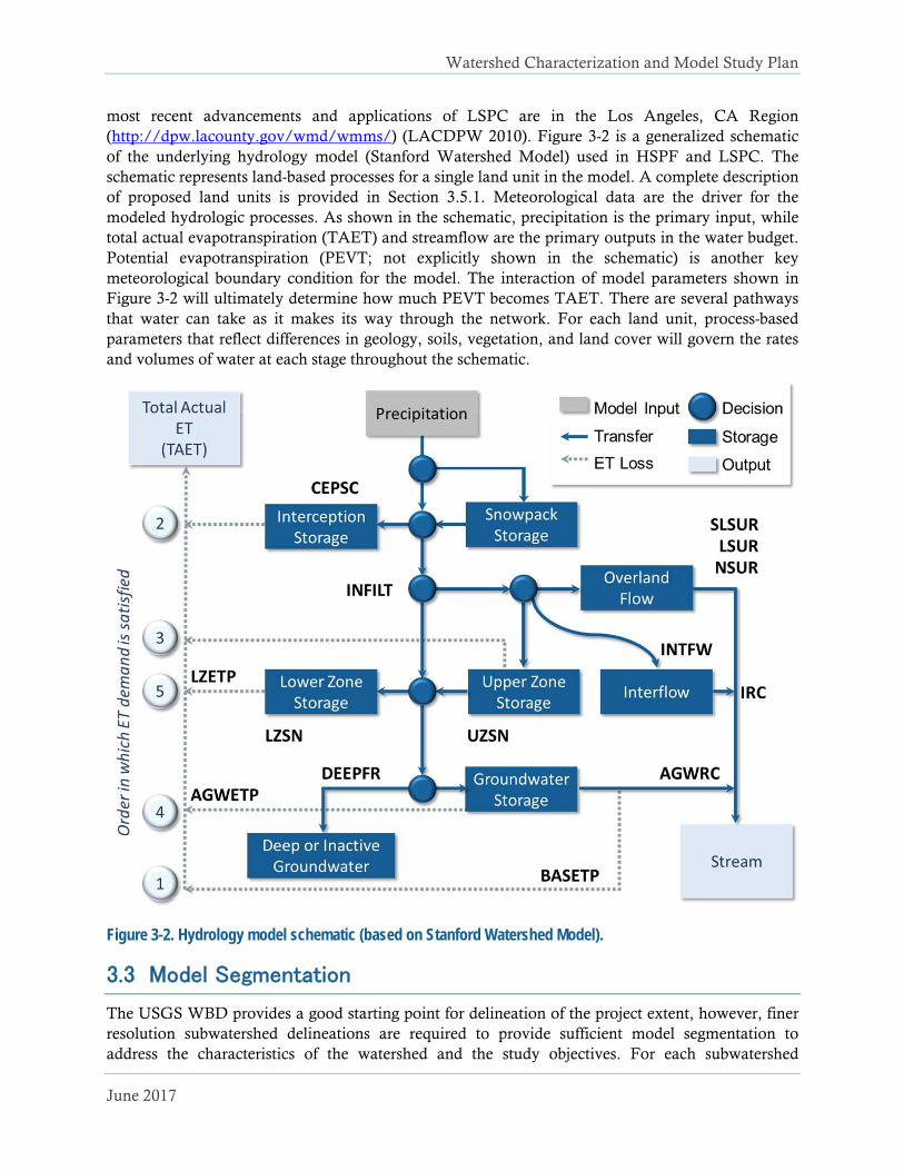
most recent advancements and applications of LSPC are in the Los Angeles, CA Region (http://dpw.lacounty.gov/wmd/wmms/) (LACDPW 2010). Figure 3-2 is a generalized schematic of the underlying hydrology model (Stanford Watershed Model) used in HSPF and LSPC. The schematic represents land-based processes for a single land unit in the model. A complete description of proposed land units is provided in Section 3.5.1. Meteorological data are the driver for the modeled hydrologic processes. As shown in the schematic, precipitation is the primary input, while total actual evapotranspiration (TAET) and streamflow are the primary outputs in the water budget. Potential evapotranspiration (PEVT; not explicitly shown in the schematic) is another key meteorological boundary condition for the model. The interaction of model parameters shown in Figure 3-2 will ultimately determine how much PEVT becomes TAET. There are several pathways that water can take as it makes its way through the network. For each land unit, process-based parameters that reflect differences in geology, soils, vegetation, and land cover will govern the rates and volumes of water at each stage throughout the schematic.
Figure 3-2. Hydrology model schematic (based on Stanford Watershed Model).
3.3 Model Segmentation
The USGS WBD provides a good starting point for delineation of the project extent, however, finer resolution subwatershed delineations are required to provide sufficient model segmentation to address the characteristics of the watershed and the study objectives. For each subwatershed
Watershed Characterization and Model Study Plan
30
represented in the LSPC model, continuous estimates of in-stream flows can be output from the model. Therefore, careful consideration will be made in the delineation of subwatersheds to correspond with POIs or other instream assessment points potentially considered for future investigations. Subwatersheds will also be delineated to correspond to locations of instream monitoring gage locations, allowing direct comparison of model-predicted flows with observed flows for model calibration and measurement of model accuracy.
A preliminary analysis was performed to delineate subwatersheds of the SFER watershed at a finer spatial resolution. This process provided a validation of HUC watershed boundaries, while considering physical characteristics and locations for model segmentation to support the study objectives and model calibration. Subwatersheds were delineated based on known physical, biological, and geologic parameters. Primary characteristics that drive boundary investigation are elevation (Figure 3-3), topography, reach connectivity, and locations of instream monitoring gages (Section 2.5). Secondary characteristics for subwatershed delineation include underlying geology, dominant climatic patterns, and dominant land cover or vegetation. Figure 3-4 presents preliminary subwatershed delineations with some of the high-level spatial considerations (CDFW 2014), as well as the locations of flow monitoring gages. Detailed descriptions and analyses of these specific watershed characteristics are found in Section 2.1 (land use), Section 2.2 (climate), and Section 2.3.4 (hydrogeology).
Following approval of the Model Study Plan and during model development, the subwatershed delineations will continue to be refined based on additional information and considerations, including such factors as:
POIs for instream flow recommendations or other future investigations. Subwatershed boundaries that correspond to additional instream flow gage locations (e.g.
CalTrout, SRF, Water Board, and UC Berkeley gages). Jurisdictional boundaries to make it possible to summarize information or representation of
management activities that are associated with specific jurisdictions. Improved management of complex stream connectivity, locations of impoundments,
diversions, or refinement of areas with large or sudden changes in elevation, topography, or other influential spatial attributes.
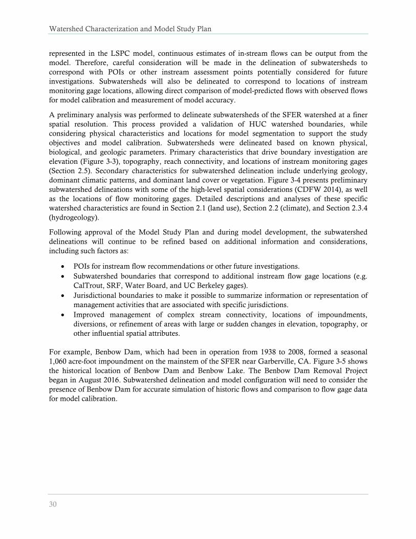
For example, Benbow Dam, which had been in operation from 1938 to 2008, formed a seasonal 1,060 acre-foot impoundment on the mainstem of the SFER near Garberville, CA. Figure 3-5 shows the historical location of Benbow Dam and Benbow Lake. The Benbow Dam Removal Project began in August 2016. Subwatershed delineation and model configuration will need to consider the presence of Benbow Dam for accurate simulation of historic flows and comparison to flow gage data for model calibration.

Watershed Characterization and Model Study Plan
June 2017
Figure 3-3. Elevation and 10-digit hydrologic boundaries of the South Fork Eel River watershed.

Watershed Characterization and Model Study Plan
32
Figure 3-4. Spatial considerations for South Fork Eel River subwatershed delineation

Watershed Characterization and Model Study Plan
June 2017
Figure 3-5. Historical location of Benbow Lake and Dam.
3.4 Meteorological Boundary Conditions
Meteorological data such as precipitation, evapotranspiration, temperature, and other climate time series are the primary forcing functions of the model—analytical considerations include data quantity and quality. Several primary and secondary meteorological data products were compiled and reviewed for this effort. Three such datasets described in further detail in the following sections include precipitation data from the Global Historical Climatology Network (GHCN), precipitation and air temperature data from the Parameter-elevation Regressions on Independent Slopes Model (PRISM), and potential evapotranspiration estimates from the California Irrigation Management Information System (CIMIS).
Watershed Characterization and Model Study Plan
34
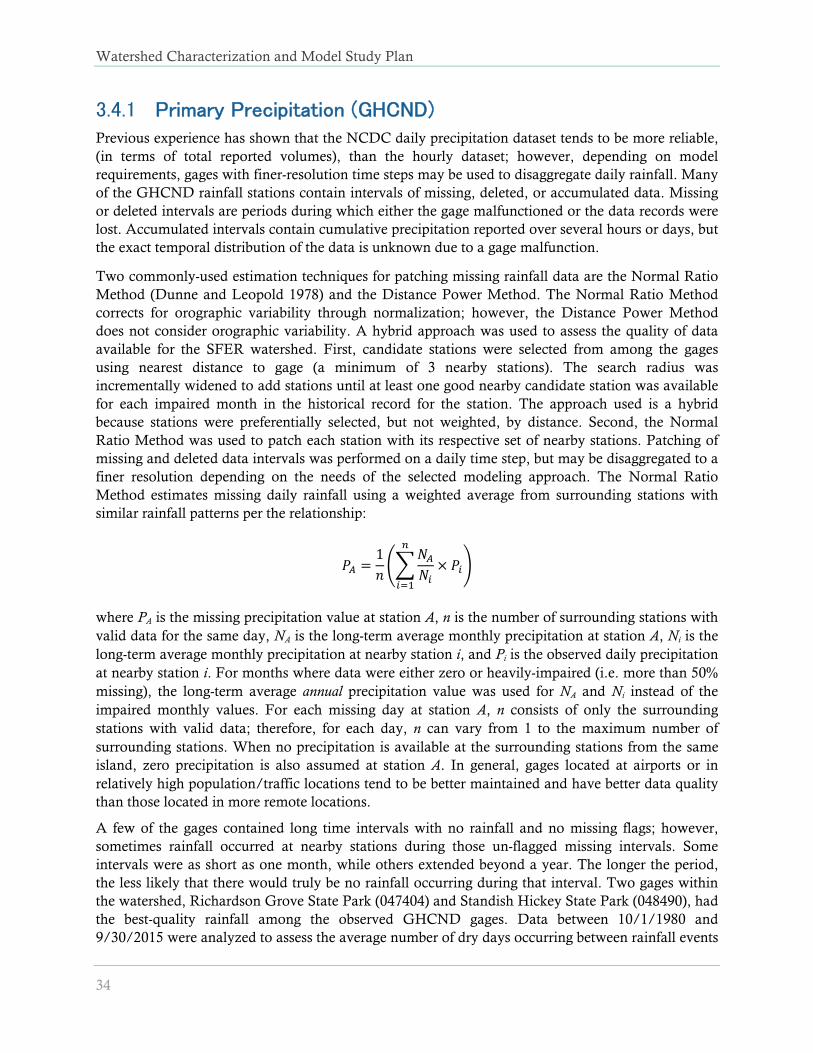
Primary Precipitation (GHCND) 3.4.1Previous experience has shown that the NCDC daily precipitation dataset tends to be more reliable, (in terms of total reported volumes), than the hourly dataset; however, depending on model requirements, gages with finer-resolution time steps may be used to disaggregate daily rainfall. Many of the GHCND rainfall stations contain intervals of missing, deleted, or accumulated data. Missing or deleted intervals are periods during which either the gage malfunctioned or the data records were lost. Accumulated intervals contain cumulative precipitation reported over several hours or days, but the exact temporal distribution of the data is unknown due to a gage malfunction.
Two commonly-used estimation techniques for patching missing rainfall data are the Normal Ratio Method (Dunne and Leopold 1978) and the Distance Power Method. The Normal Ratio Method corrects for orographic variability through normalization; however, the Distance Power Method does not consider orographic variability. A hybrid approach was used to assess the quality of data available for the SFER watershed. First, candidate stations were selected from among the gages using nearest distance to gage (a minimum of 3 nearby stations). The search radius was incrementally widened to add stations until at least one good nearby candidate station was available for each impaired month in the historical record for the station. The approach used is a hybrid because stations were preferentially selected, but not weighted, by distance. Second, the Normal Ratio Method was used to patch each station with its respective set of nearby stations. Patching of missing and deleted data intervals was performed on a daily time step, but may be disaggregated to a finer resolution depending on the needs of the selected modeling approach. The Normal Ratio Method estimates missing daily rainfall using a weighted average from surrounding stations with similar rainfall patterns per the relationship:
1
where PA is the missing precipitation value at station A, n is the number of surrounding stations with valid data for the same day, NA is the long-term average monthly precipitation at station A, Ni is the long-term average monthly precipitation at nearby station i, and Pi is the observed daily precipitation at nearby station i. For months where data were either zero or heavily-impaired (i.e. more than 50% missing), the long-term average annual precipitation value was used for NA and Ni instead of the impaired monthly values. For each missing day at station A, n consists of only the surrounding stations with valid data; therefore, for each day, n can vary from 1 to the maximum number of surrounding stations. When no precipitation is available at the surrounding stations from the same island, zero precipitation is also assumed at station A. In general, gages located at airports or in relatively high population/traffic locations tend to be better maintained and have better data quality than those located in more remote locations.
A few of the gages contained long time intervals with no rainfall and no missing flags; however, sometimes rainfall occurred at nearby stations during those un-flagged missing intervals. Some intervals were as short as one month, while others extended beyond a year. The longer the period, the less likely that there would truly be no rainfall occurring during that interval. Two gages within the watershed, Richardson Grove State Park (047404) and Standish Hickey State Park (048490), had the best-quality rainfall among the observed GHCND gages. Data between 10/1/1980 and 9/30/2015 were analyzed to assess the average number of dry days occurring between rainfall events

Watershed Characterization and Model Study Plan
June 2017
by month (Figure 3-6). The summer months of August and September were the driest months with an average of 50 dry days between rainfall events; however, the wetter months had fewer dry days between rainfall events. Based on that finding, a threshold of 50 days was selected so that any unflagged “dry” intervals greater than 50 days in the original GHCND time series would be flagged as “missing,” thereby giving them the opportunity to be patched as needed if there was rainfall observed at nearby gages. If no rainfall occurred at any of the nearby stations, the missing intervals were left as dry days.
Figure 3-6. Average number of consecutive dry days by month at two South Fork Eel River rainfall stations.
Figure 3-7 shows a summary of precipitation data near the SFER watershed that have been analyzed to fill in missing records. Table 3-1 is a tabular summary of observed vs. quality-controlled GHCND rainfall in the SFER watershed. The blue-highlighted and labeled columns are the selected gages with the best quality time series. The darker-tone portion of each station/column represents the recorded portion of annual average rainfall, while the lighter-tone portion represents the missing or extended portion of the rainfall record. The differences highlight some of the spatial and temporal quantity and quality deficiencies commonly found in observed rainfall data. The rainfall totals were also plotted against gage elevation to highlight macroscale orographic influences on rainfall totals. This two-dimensional profile does not consider the spatial locations of gages. For this reason, microscale orographic influences like aspect and rain-shadow are reflected as fluctuations in totals among gages at or near the same elevation. The SFER rainfall gages show fairly-consistent rainfall magnitude across the study area, regardless of gage elevation.

Watershed Characterization and Model Study Plan
36
Figure 3-7. GHCND precipitation gage data before and after patching missing data for the South Fork Eel River watershed.

Watershed Characterization and Model Study Plan
June 2017 37
Table 3-1. Summary of GHCND precipitation gage data before and after patching missing data for the South Fork Eel River watershed
Quality Rank
Station Name Station
ID Elevation
(ft) Evaluation Period Percent Missing
Rainfall (inches/year)
Start End Reported Adjusted Reported Adjusted
1 RICHARDSON GR ST PK 047404 500 1/1/1980 10/1/2011 14% 35% 55.98 64.04
2 STANDISH HICKEY ST PK 048490 850 1/1/1980 12/15/2010 16% 36% 54.19 64.20
3 SHELTER COVE AV 048163 246 1/1/1980 5/1/2007 26% 39% 41.46 51.46
4 HONEYDEW 1 SW 044074 370 5/7/2004 3/9/2017 66% 75% 11.90 37.10
5 MAD RIVER 7.4 SE TY0006 2,762 11/8/2008 3/9/2017 78% 82% 11.04 51.01
6 MIRANDA 4.1 SW HM0014 539 12/13/2008 3/9/2017 78% 82% 13.63 62.25
7 REDWAY 4.8 WNW HM0013 1,820 1/1/2009 2/21/2017 79% 85% 6.45 32.90
8 GARBERVILLE 2.2 SW HM0030 415 8/28/2010 3/9/2017 83% 86% 8.65 50.33
9 LAYTONVILLE 1.1 SW MD0017 1,647 10/22/2010 3/8/2017 84% 86% 8.64 51.04
10 GARBERVILLE 2.9 SW HM0031 389 9/19/2010 3/8/2017 83% 86% 8.93 52.14
11 SHELTER COVE 1.2 ENE HM0036 1,107 11/19/2010 10/16/2016 84% 87% 12.06 80.88
12 MAD RIVER RANGER STN 045244 2,675 1/1/1980 5/31/1988 79% 87% 8.09 46.92
13 REDWAY 1.8 WSW HM0044 955 3/25/2012 3/8/2017 88% 89% 6.55 55.51
14 GARBERVILLE 043320 340 1/1/1980 3/28/1985 88% 90% 8.94 62.42
15 FOREST GLEN 043130 2,339 1/2/1980 6/3/1985 87% 91% 8.06 65.21
16 REDWAY 4.3 W HM0010 612 11/1/2008 8/5/2012 90% 91% 6.75 58.57
17 LAYTONVILLE 9.8 NNW MD0022 2,078 1/27/2013 3/8/2017 90% 92% 3.47 34.70
18 WESTPORT 1.6 NNE MD0019 722 11/20/2012 3/7/2017 89% 93% 2.87 29.30
19 GARBERVILLE 1.1 WSW HM0032 510 10/24/2010 2/16/2017 84% 95% 2.77 40.31
20 REDWAY 9.9 ENE HM0056 1,577 10/31/2014 6/17/2016 95% 95% 3.30 63.22
21 CUMMINGS 042218 1,289 1/1/1980 6/12/1981 98% 98% 1.41 51.26
22 WHITETHORN 1.7 NNW HM0066 967 1/20/2016 3/9/2017 98% 99% 1.32 1.32
23 ALDERPOINT 040088 459 1/1/1980 5/25/1980 100% 100% 0.00 58.34

Watershed Characterization and Model Study Plan
38
Secondary Precipitation (PRISM) 3.4.2Secondary datasets are available to help overcome deficiencies commonly found in primary observed datasets. Behnke et al. (2016) published a first-of-its-kind study that comprehensively evaluated many of the available secondary datasets on a large geographical scale. Four key findings from their study were that: (1) temperature was represented more accurately than precipitation, (2) climate averages were more consistently predicted across datasets than weather extremes, (3) datasets with the best agreement to observed data varied geographically, (4) accuracy did not depend on spatial resolution. Behnke et al. ultimately concluded that no single secondary dataset was “best” everywhere for all variables, highlighting the need to spatially validate selected dataset against observed data to assess if it is adequately representative for the goals of the study.
PRISM was among the datasets reviewed by Behnke et al. (2016). PRISM provides a spatially-refined climatological coverage for the lower 48 contiguous United States at a 4-km spatial resolution. Developed and maintained by the PRISM Climate Group at Oregon State University (http://prism.oregonstate.edu), PRISM provides gridded estimates of event-based climate parameters including precipitation, temperature, and dew point. The algorithm uses observed point data, a digital elevation model, and other spatial datasets to capture influences such as high mountains, rain shadows, temperature inversions, coastal regions, and other complex climatic regimes (Gibson et al. 2002).
PRISM data were downloaded and summarized for the 36-year period between 10/1/1980 and 9/30/2016. Figure 3-8 shows annual average gridded PRISM rainfall coverage near the SFER watershed. The selected NCDC stations from Figure 3-6 (and labeled on Figure 3-7) were also plotted against data from the nearest PRISM centroid to validate the temporal representation of PRISM (seasonally and monthly). Figure 3-9 and Figure 3-10 are validation plots that show a close match between PRISM and observed GHCND rainfall at Richardson Grove State Park (047404) and Standish Hickey State Park (048490), respectively. This corroborates findings of others (Oswald and Dupigny-Giroux 2015; Daly et al. 2008) that PRISM can be a robust predictor of observed rainfall variability.

Watershed Characterization
June 2017
Figure 3-8. PRISM rainfall coverage for the South Fork Eel River watershed vs. selected GHCND gages.5
5 PRISM Climate Group, Oregon State University, http://prism.oregonstate.edu, created 30 Mar 2017

Watershed Characterization and Model Study Plan
40
Figure 3-9. Validation of observed GHCND (047404) vs. PRISM (333015) monthly rainfall totals.6
6 PRISM Climate Group, Oregon State University, http://prism.oregonstate.edu, created 30 Mar 2017

Watershed Characterization
June 2017
Figure 3-10. Validation of observed GHCND (048490) vs. PRISM (338636) monthly rainfall totals.7
7 PRISM Climate Group, Oregon State University, http://prism.oregonstate.edu, created 30 Mar 2017

Watershed Characterization and Model Study Plan
42
Evapotranspiration (CIMIS) 3.4.3Evapotranspiration (ET), the combined loss of water to the atmosphere from soil evaporation, plant surfaces, and plant transpiration, accounts for a large portion of a hydrologic water budget. Actual ET varies depending on vegetative cover (type, density, height) and soil conditions, making it virtually impossible to measure precisely for all environmental conditions. Nevertheless, having approximate estimates for ET is beneficial for efficient management of irrigation, which saves water, energy, and money. The (CIMIS) was established to help irrigators efficiently manage water resources. CIMIS was developed in 1982 by the DWR and the University of California, Davis. The network is composed of over 145 automated weather stations throughout California where primary weather data including temperature, relative humidity, wind speed, and solar radiation are monitored and quality-controlled. Those data are measured over standardized reference surfaces (e.g. well-watered grass or alfalfa) and are used to estimate reference evapotranspiration (ETo) using the customized Penman and Penman-Monteith equations. CIMIS has divided California into 18 zones based on long-term monthly average ETo values calculated using data from CIMIS weather stations. Figure 3-11 is a map of CIMIS zones for the SFER watershed with a plot of monthly average ETo for the mapped zones.
The western portion of the SFER watershed that is closest to the coast falls under CIMIS Zone 1, Coastal Plains Heavy Fog Belt. Less than 3 percent of the watershed falls within Zone 1. The marine cloud layer in this region reduces potential evapotranspiration (PEVT) by limiting solar radiation exposure. As shown in Figure 3-11, this results in 28 percent lower PEVT per unit area in Zone 1 compared to the rest of the watershed.
CIMIS provides relative macro-scale differences in potential ET; however actual ET varies in magnitude as a function of vegetative cover. Local practitioners in the watershed have observed regional changes to instream flows due to changes in agriculture and irrigation demand. For water budget calculations, ET coefficients are applied to PEVT data as a function of land cover to reflect stratification of vegetative impacts. Example ET coefficients are shown in Table 3-2. This approach adds spatial resolution by allowing ET to vary as a function of land cover, which also varies by subwatershed. Stratification by land cover, using coefficients like those presented in Table 3-2, adds more texture and spatial variability when calculating the ET component of the water balance.
Table 3-2. Examples of estimated stratification of modeled ET by land cover type
Cover Type Land Cover Evapotranspiration
Multiplier Rationale 1
Urban
Impervious 1.2 Above average ET (warm exposed surfaces)
Pervious 0.9 Grass or shrub vegetation
Construction 1.0 No vegetation, use standard ET rate
Rural 2
Agriculture 0.9 Grass or shrub vegetation
Barren 0.9 Grass or shrub vegetation
Forest/Wetland 0.85 Light wind, high relative humidity
Grass-Shrub 0.9 Grass or shrub vegetation
Water Water 1.0 Use evaporation rate for open water 1 Reference: Bedient and Huber, 2002. Table 1.2, Page 47. 2 Rural Land Cover categories and ET coefficients will be further refined to account for irrigation activity.

Watershed Characterization and Model Study Plan
June 2017 43
Figure 3-11. Average monthly reference evaporation for CIMIS zones in the South Fork Eel River watershed.
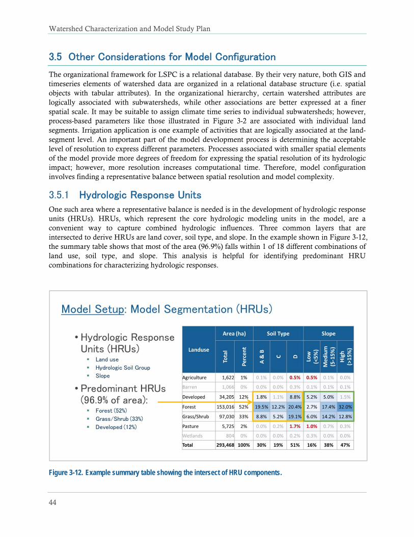
Watershed Characterization and Model Study Plan
44
3.5 Other Considerations for Model Configuration
The organizational framework for LSPC is a relational database. By their very nature, both GIS and timeseries elements of watershed data are organized in a relational database structure (i.e. spatial objects with tabular attributes). In the organizational hierarchy, certain watershed attributes are logically associated with subwatersheds, while other associations are better expressed at a finer spatial scale. It may be suitable to assign climate time series to individual subwatersheds; however, process-based parameters like those illustrated in Figure 3-2 are associated with individual land segments. Irrigation application is one example of activities that are logically associated at the land-segment level. An important part of the model development process is determining the acceptable level of resolution to express different parameters. Processes associated with smaller spatial elements of the model provide more degrees of freedom for expressing the spatial resolution of its hydrologic impact; however, more resolution increases computational time. Therefore, model configuration involves finding a representative balance between spatial resolution and model complexity.
Hydrologic Response Units 3.5.1One such area where a representative balance is needed is in the development of hydrologic response units (HRUs). HRUs, which represent the core hydrologic modeling units in the model, are a convenient way to capture combined hydrologic influences. Three common layers that are intersected to derive HRUs are land cover, soil type, and slope. In the example shown in Figure 3-12, the summary table shows that most of the area (96.9%) falls within 1 of 18 different combinations of land use, soil type, and slope. This analysis is helpful for identifying predominant HRU combinations for characterizing hydrologic responses.
Figure 3-12. Example summary table showing the intersect of HRU components.

Watershed Characterization
June 2017
Groundwater Interactions 3.5.2Groundwater pumping is one of the activities in the watershed that can have a direct impact on instream flows. Groundwater storage in LSPC (as shown in Figure 3-1) is represented as series of independent land-use-associated compartments. Recharge from the surface layers becomes either active-groundwater inflow (AGWI) or inactive groundwater inflow (IGWI), which is the volume of water that is lost to an inactive groundwater layer. The groundwater storage layer of LSPC simply provides a compartment to attenuate and release a portion of recharge back to the streams as active groundwater outflow (AGWO). Furthermore, there is no physical connection between groundwater storage compartments of adjacent land segments. A simplified groundwater model has been proposed to better represent subsurface water movement. That model would be dynamically coupled to the surface hydrology model to better represent surface-subsurface interactions and the impact of groundwater pumping on instream flows.
Groundwater Model 3.5.2.1
MODFLOW (MODFLOW-2005: Harbaugh 2005; Harbaugh et al. 2017; MODFLOW-USG: Panday et al. 2015), a widely used and accepted finite-difference flow simulator developed by USGS, will be used for developing the groundwater model. The groundwater model will adopt a basic approach based on available data and various assumptions as described below. The LSPC model will provide the AGWI to the model. The groundwater model will be used to evaluate baseflow response in stream segments resulting from changes in well-pumping. That model will be used to develop response functions that predict changes to AGWO as a function of AGWI and groundwater pumping. These functions will then replace the existing groundwater components of LSPC, as shown in Figure 3-13.
The proposed groundwater model will have a single layer encompassing the hydrologic boundaries of the SFER watershed as shown in Figure 3-4. The watershed boundary will constitute the active model domain. Lateral boundaries of the groundwater model will be no-flow conditions where the groundwater basin boundary coincides with the watershed boundary, or general head boundary conditions to allow for lateral flow to/from adjacent groundwater basins as needed. The model will be spatially partitioned into six zones: five zones representing five alluvial aquifers as listed in Section 2.3.4.1, and one zone representing the fractured rock aquifer. Spatially-distributed aquifer thickness information for the groundwater basin will need to be determined or estimated. A uniform model cell spacing of a quarter of a mile will be used initially and will be updated or refined as necessary. A transient model will be simulated to match the duration of the LSPC model. The model calibration objective for the groundwater model will be to match historical baseflow and stream depletion records as a function of recharge and pumping inputs from the watershed model.
Hydraulic conductivity and storage coefficients will be spatially varied based on the six groundwater zones as specified above. These two parameters will be estimated initially based on available descriptions of the aquifers and well-log data. The hydraulic conductivity and storage coefficients will then be subject to parameter estimation to appropriately capture: (1) gaining or losing stream reaches; (2) dry gaps; and (3) estimated baseflow rates. These stream conditions will be provided by measured data, site information, and the LSPC model. PEST (Doherty, 2008) will be used for parameter estimation. The “confined” option of MODFLOW-2005 will be implemented to
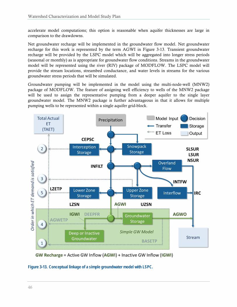
Watershed Characterization and Model Study Plan
46
accelerate model computations; this option is reasonable when aquifer thicknesses are large in comparison to the drawdowns.
Net groundwater recharge will be implemented in the groundwater flow model. Net groundwater recharge for this work is represented by the term AGWI in Figure 3-13. Transient groundwater recharge will be provided by the LSPC model which will be aggregated into longer stress periods (seasonal or monthly) as is appropriate for groundwater flow conditions. Streams in the groundwater model will be represented using the river (RIV) package of MODFLOW. The LSPC model will provide the stream locations, streambed conductance, and water levels in streams for the various groundwater stress periods that will be simulated.
Groundwater pumping will be implemented in the model using the multi-node-well (MNW2) package of MODFLOW. The feature of assigning well efficiency to wells of the MNW2 package will be used to assign the representative pumping from a deeper aquifer to the single layer groundwater model. The MNW2 package is further advantageous in that it allows for multiple pumping wells to be represented within a single aquifer grid-block.
Figure 3-13. Conceptual linkage of a simple groundwater model with LSPC.

Watershed Characterization
June 2017
Groundwater Pumping 3.5.2.2
Currently, well location data are available for Mendocino County. Approximate locations are available for a total of 797 wells in the Mendocino County, of which, location accuracy for 65 wells have a tract number placing these within approximately one-eighth of a mile accuracy, 718 wells have a section number available placing these within approximately half-mile accuracy, and 14 wells have only a township and range number placing these within a three-mile accuracy. Figure 3-14 shows the available pumping well locations and spatial accuracy. It is assumed that a similar dataset will be provided by the Water Board for the remainder of the model domain in Humboldt County.
Pumping rates for wells will be estimated based on their designated use and either the population that the well serves or irrigation usage, and will be consistent between the groundwater model and the LSPC model. Pumping rate estimates will ultimately be aggregated by subwatershed as a function of consumptive uses associated with groundwater sources.
Historical records will be evaluated to determine a representative steady-state starting period for the model. The model will then be run in transient mode through water year 2016, in accordance with the time period simulated by the LSPC model. Quarterly stress periods will be used to vary recharge and pumping. Recharge output from the LSPC model as well as pumping estimates will be aggregated into quarterly periods for input to the groundwater model. The steady-state model will be calibrated to baseflow estimates for various stream reaches, including gaining or losing conditions and estimates of dry gap locations. The transient model will be calibrated to the general changes in these conditions resulting from changes in groundwater recharge and pumping.
The approach discussed above will provide a preliminary assessment of groundwater pumping on instream flows. The model may be applied to evaluate the impact of reduced recharge to the groundwater domain or increased pumping from groundwater wells on baseflow to streams. The model is a first-step towards a fully coupled surface water – groundwater system and provides the foundation for increasing complexity of the modeling or coupling, if warranted. Therefore, the system of models is well suited for supporting the current study objectives, while providing flexibility for future refinements to address other investigations of the overall water balance of the SFER watershed.
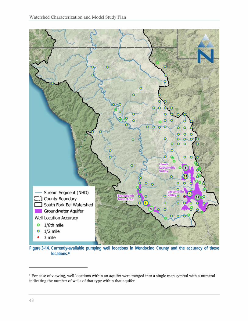
Watershed Characterization and Model Study Plan
48
Figure 3-14. Currently-available pumping well locations in Mendocino County and the accuracy of these
locations.8
8 For ease of viewing, well locations within an aquifer were merged into a single map symbol with a numeral indicating the number of wells of that type within that aquifer.

Watershed Characterization
June 2017
Coupled Surface-Groundwater Model 3.5.2.3
The AGWO component of LSPC has an attenuated and delayed response compared to the surface runoff (SURO) and interflow outflow (IFWO) components. Coupling LSPC to the simplified groundwater model involves some spatial and temporal aggregation. Because groundwater interactions have a longer temporal response period (i.e. monthly or seasonal) compared to surface interactions, it is reasonable to aggregate recharge inputs to a monthly time step at the subwatershed scale. Using best available information to characterize the groundwater basin, the groundwater model will be calibrated to match observed trends in stream depletion. As illustrated in Figure 3-15, the goal of this effort is to develop groundwater response functions that can be used to predict changes in AGWO as a function of AGWI and groundwater pumping rates. Outputs from the groundwater model would be translated back to an hourly temporal scale when linking to the LSPC model. The resulting outputs would be applied in the same way as the original LSPC model prior to coupling.
Figure 3-15. Development of groundwater response functions for HSPF using and a simple groundwater model.
3.6 Process for Model Calibration and Validation
The modeling approach is designed to follow internationally-recognized modeling protocols and conventions. For example, the USEPA (2002) guidance for Quality Assurance Project Plans (QAPP) for modeling refers to calibration as the configuration and refinement of the analytical instruments

Watershed Characterization and Model Study Plan
50
that will be used to generate analytical data. The “instrument” is the predictive tool (i.e. the model) that is to be developed and/or applied. Figure 3-16 is a schematic describing a process for model calibration that aims to minimize the propagation of uncertainty. This process builds upon the model development cycle and elements of data quality control previously shown in Figure 3-1. Through development of the Model Study Plan, the analysis of weather data was initiated and discussed in Section 3.4. Snowfall is not considered to be a factor for the SFER watershed, and will not be addressed in the Model Study Plan. Therefore, the calibration process discussed herein will focus on the land hydrology and stream transport components of Figure 3-16.
Figure 3-16. Process for model calibration to minimize propagation of uncertainty.
The demonstration of model calibration is key to the model development process, as it forms the basis for establishing the degree of uncertainty in model predictions and the reliability of the model to base management decisions. Models will be deemed acceptable when they can simulate field data within predetermined statistical measures. In evaluating a given calibration, it will be useful to look at several parameters. After weather data and meteorological boundary conditions are well established, a top-down weight of evidence approach will progress as follows: (1) calibrate background conditions, (2) add intermediate mixed land use areas, and (3) aggregate all sources via routing to a downstream location for comparison with co-located flow data. Figure 3-17 is a schematic showing the parameterization and calibration sequence for land hydrology. Unit-area results from this step will be summarized and compared relative to each other and against representative published literature values. This step will provide an early opportunity to identify possible errors, anomalies, or other unrepresentative behavior prior to aggregation, instream routing, and transport.

Watershed Characterization
June 2017
Figure 3-17. Model parameterization and calibration sequence for land hydrology.
Figure 3-18 is a schematic of stream transport model parameterization and calibration sequence. Outputs from land hydrology will be aggregated and routed to the stream transport model, where other features such as impoundments, diversions, withdrawals, and point sources may influence the water balance. Using the most representative spatial and temporal data inputs to characterize elements at this stage will further minimize propagation of uncertainty through the model.
Figure 3-18. Model parameterization and calibration sequence for waterbodies and stream transport.
A two-phase weight-of-evidence approach is proposed to guide LSPC’s calibration. In the first phase, the model will be set up with typical parameter values, such as those suggested in BASINS Technical Note 6: Estimating Hydrology and Hydraulic Runoff Parameters (USEPA 2006). Land-level hydrology will be calibrated to best reflect the central tendency of land use runoff using supporting information such as geology, soil type, canopy cover, and surface cover conditions. After the model has been calibrated to reflect overall trends and reasonable process dynamics, the second phase involves fine tuning the parameters and calculating various error statistics to find a most appropriate calibration within the range of acceptable parameter values to characterize instream transport routing processes in conjunction with other natural or anthropogenic activities, as applicable.

Watershed Characterization and Model Study Plan
52
For hydrologic calibration of HSPF, performance targets have been specified in various literature sources, including Donigian et al. (1984), Lumb et al. (1994), and Donigian (2000). The LSPC model is functionally identical to the HSPF model. Based on those literature sources, performance targets for simulation of the water balance components are summarized in Table 3-3. The relative error is the ratio of the absolute mean error to the mean of the observations and is expressed as a percent. Model performance will be deemed fully acceptable where a performance evaluation of “Good” or “Very Good” is attained. Nevertheless, every calibration outcome will be explained, with some insights and rationale provided for both “Very Good” to “Poor” calibration metrics in light of the top-down weight-of-evidence approach described above. If these levels are not attained, an analysis of sources of uncertainty and implications for model usability will be conducted.
Table 3-3. Performance targets for HSPF hydrology simulation (modeled vs. observed)
Model Component Very Good Good Fair Poor
Error in Total Volume < 5% 5-10% 10-15% > 15%
Error in 50% Lowest Flow Volumes < 10% 10-15% 15-25% > 25%
Error in 10% Highest Flow Volumes < 10% 10-15% 15-25% > 25%
Error in Storm Volumes < 10% 10-15% 15-25% > 25%
Winter Volume Error <15% 15-30% 30-50% >50%
Spring Volume Error <15% 15-30% 30-50% >50%
Summer Volume Error <15% 15-30% 30-50% >50%
Fall Volume Error <15% 15-30% 30-50% >50%
R2 Daily >= 0.8 >= 0.7 >= 0.6 <0.6
R2 Monthly >= 0.85 >= 0.75 >= 0.65 < 0.65
The top-down weight-of-evidence based approach for model calibration will use a variety of graphical and statistical points of comparison. Figure 3-19 summarizes the long-term calibrated water balance for an example watershed. Figure 3-20 shows example calibrated surface runoff and evapotranspiration summaries by land use category. Some sample timeseries plots of modeled versus observed streamflow timeseries are also shown in Figure 3-21 and Figure 3-22.
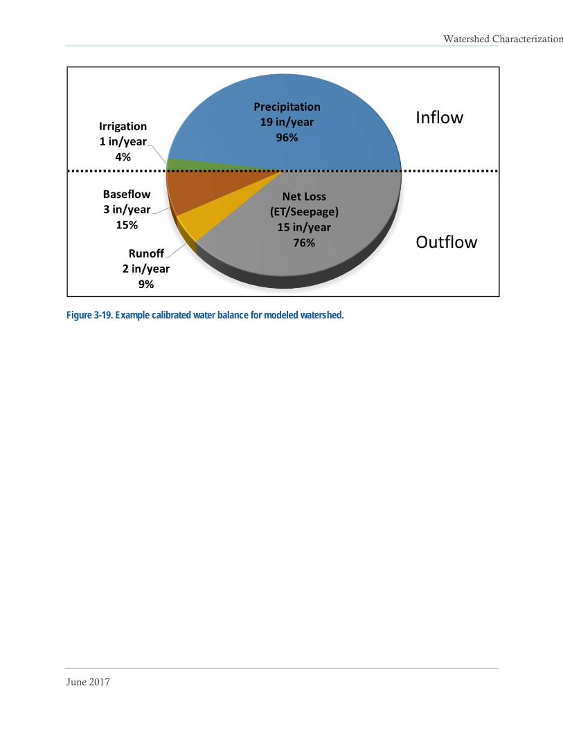
Watershed Characterization
June 2017
Figure 3-19. Example calibrated water balance for modeled watershed.

Watershed Characterization and Model Study Plan
54 June 2017
Figure 3-20. Example surface runoff and evapotranspiration summaries by land use category.

Watershed Characterization and Model Study Plan
June 2017 55
Figure 3-21. Examples of daily and monthly modeled versus observed streamflow.
0
2
4
6
8
10
12
14
16
18
200
1,000
2,000
3,000
4,000
5,000
6,000
7,000
8,000
Precipitation (in.)
Stream
flow (cfs)
Precipitation (in.) Observed: Malibu Creek Below Cold Creek Modeled Streamflow
0
10
20
30
40
50
600
1
2
3
4
5
6
7
8
9
10
10/1/2000
1/1/2001
4/1/2001
7/1/2001
10/1/2001
1/1/2002
4/1/2002
7/1/2002
10/1/2002
1/1/2003
4/1/2003
7/1/2003
10/1/2003
1/1/2004
4/1/2004
7/1/2004
10/1/2004
1/1/2005
4/1/2005
7/1/2005
10/1/2005
1/1/2006
4/1/2006
7/1/2006
10/1/2006
1/1/2007
4/1/2007
7/1/2007
10/1/2007
1/1/2008
4/1/2008
7/1/2008
10/1/2008
1/1/2009
4/1/2009
7/1/2009
10/1/2009
1/1/2010
4/1/2010
7/1/2010
Precipitation (in.)
Norm
alized Streamflow (in.)
Daily Streamflow
Monthly Streamflow
(Normalized by Area)
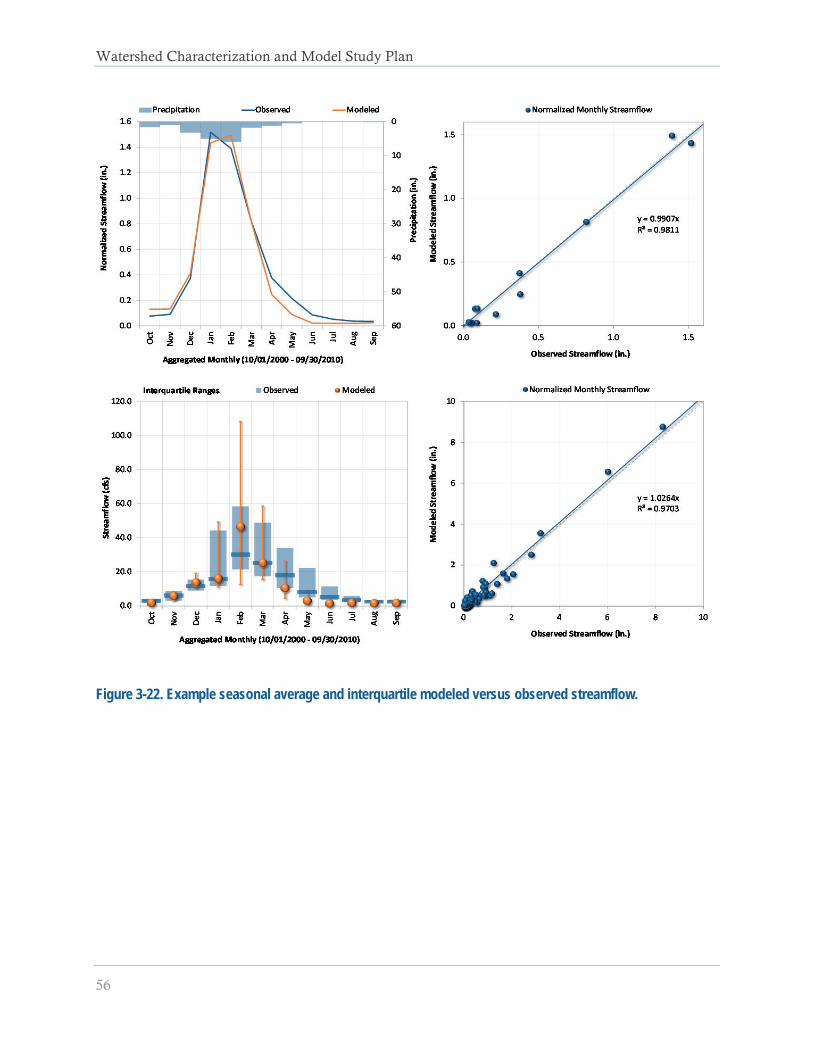
Watershed Characterization and Model Study Plan
56
Figure 3-22. Example seasonal average and interquartile modeled versus observed streamflow.

Watershed Characterization
June 2017
Model Validation 3.6.1Validation is defined as testing the model through application to a set of data not used to develop the calibration. Model validation is an extension of the calibration process. Its purpose is to test the predictive ability of the calibrated model, identify aspects of the calibration that might need further refinement, and provide information on prediction uncertainty.
Although several approaches can be used to validate a model, perhaps the most effective way is to use only a portion of the available observed values for calibration and use the rest for validation. Once final calibration parameters are developed, simulation will be performed for the remaining period of observed values and the goodness-of-fit between recorded and simulated values will be reassessed. Such a split-sample calibration and validation procedure is commonly used for evaluating model robustness. Figure 3-23 presents an overview of the model validation process which begins with testing the locked down model response for alternative points in space and time (snow is likely not relevant for the SFER watershed).
Figure 3-23. Process for model validation and identification of data gaps.
3.7 Model Scenarios to Investigate Study Objectives
Based on the calibrated model, analyses will be performed for modeled streamflows at various locations and POIs throughout the watershed to address the study objectives. Assessment will be performed for various flow regimes, including historic peak flows, low flows, annual volumes during various periods, and unimpaired flows. The analysis will support the generation of flow “return periods,” or the statistical likelihood that various high and low percentile flows occur within various stream and tributary reaches of each watershed.
Figure 3-24 presents an example flow-duration curve analysis to define a critical condition flow rate during dry weather, with a focus on summer conditions. A representative watershed model can provide mechanistically-derived estimates of hydrological conditions where there are gaps in spatial or temporal resolution.

Watershed Characterization and Model Study Plan
58
Figure 3-24. Example flow-duration curve analysis to define summer low-flow critical conditions.
4. REFERENCES
Asarian, J.E. 2015. Long-term Streamflow and Precipitation Trends in the Eel River Basin. Prepared by Riverbend Sciences for Friends of the Eel River, Arcata, CA. 30p.
Bauer, S., J. Olson, A. Cockrill, M. van Hattem, L. Miller, M. Tauzer, and G. Leppig. 2015. Impacts of Surface Water Diversions for Marijuana Cultivation on Aquatic Habitat in Four Northwestern California Watersheds. PLoS ONE 10:e0120016. doi: 10.1371/journal.pone.0120016.
Bauer, S. 2015. Marijuana Cultivation in the Mad River Watershed. Presentation to the Humboldt Bay Municipal Water District. California Department of Fish and Wildlife, Eureka, CA.
Bicknell, B. R., J. C. Imhoff, A. S. Donigian, R. C. Johanson. 1997. Hydrological Simulation Program – FORTRAN (HSPF), User’s Manual For Release 11. EPA – 600/R-97/080. U.S. Environmental Protection Agency, Athens, GA.
Brooks P.D., Chorover J., Fan Y., Godsey S.E., Maxwell R.M., McNamara J.P., and Tague C. 2015. Hydrological partitioning in the critical zone: Recent advances and opportunities for developing transferable understanding of water cycle dynamics. Water Resources Research 51 (9): 6973-6987.
Watershed Characterization
June 2017
Brown, W., and J. Ritter. 1971. Sediment transport and turbidity in the Eel River basin, California. U.S. Geological Survey Water Supply Paper 1986, 70 p.
CDFW (California Department of Fish and Wildlife). 2014. South Fork Eel River Watershed Assessment. Coastal Watershed Planning and Assessment Program. California Department of Fish and Wildlife.
CDFW (California Department of Fish and Wildlife). 2016. Study Plan: Habitat and Instream Flow Evaluation for the Anadromous Salmonids in the South Fork Eel River and Tributaries, Humboldt and Mendocino Counties. CDFW Instream Flow Program, Sacramento, CA.
CDMG (California Division of Mines and Geology). 1999. North Coast Watersheds Mapping by the California Department of Forestry as part of the North Coast Watershed Assessment Program.
Doherty, J., PEST: Model-Independent Parameter Estimation, Watermark Numerical Computing, Brisbane, Australia, 2008. http://pesthomepage.org/
Donigian, A.S. Jr. 2000. HSPF Training Workshop Handbook and CD. Lecture #19. Calibration and Verification Issues. Prepared for U.S. Environmental Protection Agency, Office of Water, Office of Science and Technology, Washington, DC.
Dunne, T. and L.B. Leopold. 1978. Water in Environmental Planning. W.H. Freeman and Company, New York.
Eel River Forum. 2016. The Eel River Action Plan: A Compilation of Information and Recommended Actions. Eel River Forum, California Trout, San Francisco, CA.
Farrar, C. 1986. Ground-water resources in Mendocino County, California. USGS Water Resources Investigations REpor 85-4258. July
Field, J.P., D.D. Breshears, D.J. Law, J.C. Villegas, L. López-Hoffman, P.D. Brooks, J. Chorover, G.A. Barron-Gafford, R.E. Gallery, M.E. Litvak, Rebecca A. Lybrand, J.C. McIntosh, T. Meixner, G-Y. Niu, S.A. Papuga, J.D. Pelletier, C.R. Rasmussen and P.A. Troch. 2014. Critical Zone Services: Expanding Context, Constraints, and Currency beyond Ecosystem Services. Vadose Zone Journal. doi:10.2136/vzj2014.10.0142.
Flint, L.E. and Flint, A.L. 2014. California Basin Characterization Model: A Dataset of Historical and Future Hydrologic Response to Climate Change. U.S. Geological Survey Data Release, doi:10.5066/F76T0JPB.
Foster, M. 2010. Knickpoints in the tributaries of the South Fork Eel River, Northern California. Thesis presented to faculty of Humboldt State University, Environmental Systems : Geology. May.
Harbaugh, A.W. 2005. MODFLOW-2005, the U.S. Geological Survey modular ground-water model -- the Ground-Water Flow Process: U.S. Geological Survey Techniques and Methods 6-A16.
Harbaugh, A.W., Langevin, C.D., Hughes, J.D., Niswonger, R.N., and Konikow, L. F. 2017. MODFLOW-2005 version 1.12.00, the U.S. Geological Survey modular groundwater

Watershed Characterization and Model Study Plan
60
model: U.S. Geological Survey Software Release, 03 February 2017, http://dx.doi.org/10.5066/F7RF5S7G
Jayko, A.S., Blake, M.C., McLaughlin, R.J., Ohlin, H.N., Ellen, S.D., and Kelsey, H.M. 1989. Reconnaissance Geologic Map of the Covelo 30-by 60-Minute Quadrangle, Northern California: U.S. Geological Survey Miscellaneous Field Investigation Map MF-2001, scale 1:100 000.
LaVen, R.D. 1987. A late Pleistocene and Holocene erosion history of the South Fork of the Eel River. Humboldt State University Foundation. Arcata, CA.
Kelsey, H.M. 1977. Landsliding, Channel Changes, Sediment Yield and Land Use in the Van Duzen River Basin, North Coastal California, 1941–1975 [Ph.D. thesis]: Santa Cruz, University of California, 370 p.
Kelsey, H.M. and Carver, G.A. 1988. Late Neogene and Quaternary tectonics associated with northward growth of the San Andreas transform fault, northern California, Journal of Geophysical Research, 93, (B5) 4797-4819.
Klein, R. and B. Eastwood. 2016. Preliminary Low Flow Stream Discharge Monitoring Report for the Redwood Creek Watershed. September 14, 2016. Prepared for the Salmonid Restoration Federation.
LACDPW (Los Angeles County Department of Public Works). 2010. Los Angeles County Watershed Model Configuration and Calibration—Part I: Hydrology. Prepared for LACDPW, Watershed Management Division, Los Angeles County, CA, by Tetra Tech, Pasadena, CA.
Lisle, T. 1981. Recovery of aggraded stream channels at gaging stations in northern California and southern Oregon. Davis, T. R. H.; Pearce, A. J., eds. Erosion and sediment transport in Pacific Rim steeplands, symposium; IAHS-AISH Publ. 132, 189-200.
Lisle, T. 1982. Effects of aggradation and degradation on riffle-pool morphology in natural gravel channels, northwestern California. Water Resources Research 18 (6), 1643–1651.
Lisle, T. 1990. The Eel River, Northwestern California: high sediment yields from a dynamic landscape. Pages 311–314 in M. G. Wolman and H. G. Riggs, editors. Surface water hydrology, v O-1. The geology of North America. Geological Society of America.
Lumb, A.M., R.B. McCammon, and J.L. Kittle Jr. 1994. User’s Manual for an Expert System (HSPEXP) for Calibration of the Hydrological Simulation Program–FORTRAN. Water-Resources Investigations Report 94-4168. U.S. Geological Survey, Reston, VA.
Mackey, B., and J. Roering. 2011. Sediment yield, spatial characteristics, and the long-term evolution of active earthflows determined from airborne LiDAR and historical aerial photographs, Eel River, California. Geological Society of America Bulletin. doi:10.1130/B30306.1.1.
McKay, L., Bondelid, T., Dewald, T., Johnston, J., Moore, R., and Rea, A., NHDPlus Version 2: User Guide, 2012

Watershed Characterization
June 2017
McLaughlin, R. J., S. D. Ellen, et al. (2000). Geology of the Cape Mendocino, Eureka, Garberville, and Southwestern part of the Hayfork 30 X 60 minute quadrangles and adjacent offshore area, Northern California, U.S. Department of the Interior, United States Geological Survey: 27 p.
NOAA Fisheries (National Marine Fisheries Service). 2014. Final Recovery Plan for the Southern Oregan/ Northern California Coast Evolutionarily Significant Unit of Coho Salmon (Oncorhynchus kisutch). National Marine Fisheries Service, Arcata, CA.
National Research Council. 2001. Basic Research Opportunities in Earth Science. Washington, DC: The National Academies Press.
Panday, Sorab, Langevin, C.D., Niswonger, R.G., Ibaraki, Motomu, and Hughes, J.D. 2015. MODFLOW-USG version 1.3.00: An unstructured grid version of MODFLOW for simulating groundwater flow and tightly coupled processes using a control volume finite-difference formulation: U.S. Geological Survey Software Release, 01 December 2015.
Rempe, D. and W. Dietrich. 2014. A bottom-up control on fresh-bedrock topography under landscapes. Proceedings of the National Academy of Sciences. Vol. 111, No. 18. May.
Salve, R. D. Rempe, and W. Dietrich. 2012. Rain, rock moisture dynamics, and the rapid response of perched groundwater in weathered, fractured argillite underlying a steep hillslope. Water Resources Research, VOL. 48, W11528, doi:10.1029/2012WR012583.
Short, D. 1984. Cuneo Creek, Land Use History and Changes in Channel Morphology.
U.S. Army Corps of Engineers. 1999. Eel and Van Duzen Rivers, General Assessment of Historical Change in Channel Morphology. San Francisco, CA.
Tetra Tech and USEPA (U.S. Environmental Protection Agency). 2002. The Loading Simulation Program in C++ (LSPC) Watershed Modeling System – User’s Manual. Tetra Tech, Fairfax, VA, and U.S. Environmental Protection Agency, Washington, DC.
USEPA (United States Environmental Protection Agency). 2000. BASINS Technical Note 6: Estimating Hydrology and Hydraulic Parameters for HSPF. EPA-823-R00-012. USEPA, Office of Water, Washington D.C. July 2000.
USEPA (U.S. Environmental Protection Agency). South Fork Eel River Total Maximum Daily Loads for Sediment and Temperature: 57.
USEPA (U.S. Environmental Protection Agency). 2000. BASINS Technical Note 6: Estimating Hydrology and Hydraulic Parameters in HSPF – EPA-823-R00-012. U.S. Environmental Protection Agency, Office of Water, Washington, DC.
USEPA (United States Environmental Protection Agency). 2002. Guidance for Quality Assurance Project Plans for Modeling – EPA QA/G-5M. EPA/240/R-02/007. United States Environmental Protection Agency. Office of Environmental Information. December 2002.
USEPA (U.S. Environmental Protection Agency). 2006. BASINS Technical Note 8: Sediment Parameter and Calibration Guidance for HSPF– June 2006. U.S. Environmental Protection Agency, Office of Water, Washington, DC.
Watershed Characterization and Model Study Plan
62
USEPA (U.S. Environmental Protection Agency). 2006a. Data Quality Assessment: A Reviewers Guide – EPA QA/G-9R. EPA/240/B-06/002. U.S. Environmental Protection Agency, Office of Environmental Information, Washington, DC.
USEPA (U.S. Environmental Protection Agency). 2006b. Data Quality Assessment: Statistical Methods for Practitioners – EPA QA/G-9S. EPA/240/B-06/003. U.S. Environmental Protection Agency, Office of Environmental Information, Washington, DC.
USEPA (U.S. Environmental Protection Agency). 2006c. Guidance on Systematic Planning Using the Data Quality Objectives Process – EPA QA/G-4. EPA/240/B-06/001. U.S. Environmental Protection Agency, Office of Environmental Information, Washington, DC.