CALIPSO QualityStatements

Lidar Level 2 Cloud andAerosol Layer ProductsVersion Releases: 3.01,

3.02

Introduction | Documentation and References | Standard and Expedited Data Set Definitions | CALIPSO Lidar Level 2 Data Products |Overview | Revision Summary: Version 3.02 and Version 3.01

Introduction

This document provides a high-level quality assessment of the cloud and aerosol layer products derived from the CALIPSO lidarmeasurements, as described in section 2.4 of the CALIPSO Data Products Catalog (Version 3.2) (PDF). As such, it represents the minimuminformation needed by scientists and researchers for appropriate and successful use of these data products. We strongly suggest that allauthors, researchers, and reviewers of research papers review this document periodically, and familiarize themselves with the latest statusbefore publishing any scientific papers using these data products.

These data quality summaries are published specifically to inform users of the accuracy of CALIOP data products as determined by theCALIPSO Science Team and Lidar Science Working Group (LSWG). This document is intended to briefly summarize key validation results;provide cautions in those areas where users might easily misinterpret the data; supply links to further information about the data products andthe algorithms used to generate them; and offer information about planned algorithm revisions and data improvements.

The primary geophysical variables reported by Cloud and Aerosol Layer Products are the spatial locations of layers (e.g., layer base and topaltitudes), the surrounding meteorological conditions (e.g., temperature and pressure) and a number of measured and derived opticalproperties. Optical properties that are directly measured include integrated attenuated backscatter, volume depolarization ratio, andattenuated total color ratio. Derived optical properties are those that can only be obtained via application of the CALIPSO extinction retrieval.Optical depth is the primary derived optical property reported in the Layer Products. Others include ice water path, particulate depolarizationratio, and particulate color ratio. PLEASE NOTE: Users of those CALIOP parameters that are produced by or otherwise depend on theextinction retrieval(s) should read and thoroughly understand the information provided in the Profile Products Data Quality Summary. Thissummary contains an expanded description of the extinction retrieval process from which the layer optical depths are derived, and providesessential guidance in the appropriate use of all CALIOP extinction-related data products.

Data Product Maturity

Because validation for different parameters can require different levels of effort, and because the uncertainties inherent in some retrievals canbe substantially larger than in others, the maturity levels of the parameters reported in the different layer products files are not uniform.Therefore, within this document, maturity levels are provided separately for each scientific data set (SDS) included with the data files. Thedata product maturity levels for the CALIPSO layer products are defined in the table below.

Maturity Level DefinitionsBeta: Early release products for users to gain familiarity with data formats

and parameters. Users are strongly cautioned against theindiscriminate use of these data products as the basis forresearch findings, journal publications, and/or presentations.

Provisional: Limited comparisons with independent sources have been made andobvious artifacts fixed.

Validated Stage 1: Uncertainties are estimated from independent measurements atselected locations and times.

Validated Stage 2: Uncertainties are estimated from more widely distributed independentmeasurements.

Validated Stage 3: Uncertainties are estimated from independent measurementsrepresenting global conditions.

External: Data are not CALIPSO measurements, but instead are eitherobtained from external sources (e.g., the Global Modeling andAssimilation Office (GMAO)) or fixed constants in the CALIPSOretrieval algorithm (e.g., the 532 nm calibration altitude).

As a general (but not immutable) rule, the parameters in the cloud and aerosol layer products whose derivation depends wholly or in part onthe extinction retrieval are assigned a product maturity level of provisional. Those products derived from the layer detection and sceneclassification algorithms only are designated as ValStage1.

Documentation and References

Algorithm Theoretical Basis Documents (ATBDs)

PC-SCI-202.01 - Mission, Instrument, and Algorithms Overview (PDF)PC-SCI-202.02 - Feature Detection and Layer Properties Algorithms (PDF)PC-SCI-202.03 - Scene Classification Algorithms (PDF)PC-SCI-202.04 - Extinction Retrieval Algorithms (PDF)

General References

PC-SCI-503 : CALIPSO Data Products Catalog (Version 3.2) (PDF)Data analysis overview: Fully automated analysis of space-based lidar data: an overview of the CALIPSO retrieval algorithms and dataproducts (PDF)CALIPSO algorithm papers published in a special issue of the Journal of Atmospheric and Oceanic TechnologyPeer-reviewed CALIPSO validation papersAdditional peer-reviewed publications discussing scientific applications and studies using CALIPSO dataRecent conference proceedings covering a broad range of CALIPSO-related science and data analysis topicsCALIPSO Data Read Software

Standard and Expedited Data Set Definitions

Standard Data Sets:Standard data processing begins immediately upon delivery of all required ancillary data sets. The ancillary data sets used in standardprocessing (e.g., GMAO meteorological data and data from the National Snow and Ice Data Center) must be spatially and temporally matchedto the CALIPSO data acquisition times, and thus the time lag latency between data onboard acquisition and the start of standard processingcan be on the order of several days.The data in each data set are global, but are produced in files by half orbit, with the day portion of an orbit in one file and the night portion ofthe orbit in another.

Expedited Data Sets:Expedited data are processed as soon as possible after following downlink from the satellite and delivery to LaRC. Latency between onboardacquisition and analysis expedited processing is typically on the order of 6 to 28 hours. Expedited processing uses the most recently currentavailable set of ancillary data (e.g., GMAO meteorological profiles) and calibration coefficients available, which may lag the CALIPSO dataacquisition time/date by several days.Expedited data files contain at the most, 90 minutes of data. Therefore, each file may contain both day and night data.NOTE: Users are strongly cautioned against using Expedited data products as the basis for research findings or journalpublications. Standard data sets only should be used for these purposes.

The differences between expedited processing and standard processing are explained in more detail in "Adapting CALIPSO ClimateMeasurements for Near Real Time Analyses and Forecasting" (PDF).

CALIPSO Cloud and Aerosol Layer Products

Overview

The CALIPSO Cloud and Aerosol Layer Products are built around two tightly coupled data types. The first of these is a set of columnproperties, which describe the temporal and spatial location of the vertical column (or, for averaged data, curtain) of atmosphere beingsampled. Column properties include satellite position data and viewing geometry, information about the surface type and lighting conditions,and the number of features (e.g., cloud and/or aerosol layers) identified within the column. For each set of column properties, there is anassociated set of layer properties. These layer properties specify the spatial and optical characteristics of each feature found, and includequantities such as layer base and top altitudes, integrated attenuated backscatter, layer-integrated volume depolarization ratio, and opticaldepth. Below we provide brief descriptions of each of the column properties and the layer properties. Where appropriate, we also provide anassessment of the quality and accuracy of the data in the current release.

The layer products are generated at three different spatial resolutions.

The 1/3 km layer products report cloud detection information obtained at the highest spatial resolution of the lidar: 1/3 km horizontallyand 30-m vertically. Due to constraints on CALIPSO's downlink bandwidth, this full resolution data is only available from ~8.3 kmabove mean sea level, down to -0.5 km below sea level.

The 1 km layer products report cloud detection information obtained at a horizontal resolution of 1 km, over a vertical range extendingfrom ~20.2 km above mean sea level, down to -0.5 km below sea level.

The 5 km layer products report (separately) cloud and aerosol detection information on a 5 km horizontal grid. At present there is noseparate stratospheric data product. Stratospheric features are recorded in the 5 km aerosol product.

Users should be aware that while the 5 km layer products are reported on a uniform 5 km grid, the amount of horizontal averagingrequired to detect a layer may exceed 5 km. For example, detection of subvisible cirrus during daylight operations may requireaveraging to 20 km or even 80 km horizontally. In these cases, the layer properties of the feature detected are replicated as necessaryto span the full extent of the averaging interval required for detection. For example, the layer properties for an aerosol layer that couldonly be detected after averaging over 20 km horizontally will be repeated over four consecutive 5 km columns.

The fundamental data product provided by the CALIPSO layer products is the vertical location of cloud and aerosol layer boundaries. All otherlayer properties -- e.g., integrated attenuated backscatters and layer two-way transmittances -- are computed with reference to theseboundaries. To make proper use of the CALIPSO layer products, all users must be aware of the uncertainties inherent in the fully automatedrecognition of layer boundaries. Note too that clouds and aerosols are reported separately in the CALIPSO layer products. Therefore, toobtain a complete representation of all features detected within any region, users must use both the cloud and the aerosol layer products.

In the remainder of this document we provide brief descriptions of the individual parameters contained within the layer products files.Accompanying these descriptions are qualitative summaries of the product maturity level. Where appropriate, specific quality flags areincluded in the data products, and these too are described in some detail. The data descriptions are grouped into several major categories, asfollows:

Column Time ParametersColumn Geolocation ParametersColumn Spacecraft OrientationColumn Surface PropertiesColumn Meteorological DataColumn Optical PropertiesColumn QA InformationLayer Spatial PropertiesLayer Meteorological PropertiesLayer Measured Optical PropertiesLayer Derived Optical PropertiesLayer QA InformationFile Metadata Parameters

Column Time Parameters

Day Night FlagThis field indicates the lighting conditions at an altitude of ~24 km above mean sea level; 0 = day, 1 = night.

Profile TimeTime expressed in International Atomic Time (TAI). Units are in seconds, starting from January 1, 1993. Times reported in the 1/3 kmlayer products are for the individual laser pulses from which the layer statistics were derived. Times reported in the 1 km layerproducts represent the temporal midpoint of the three laser pulses averaged to generate the 1 km horizontal resolution. For the 5 kmlayer products, three values are reported: the time for the first pulse included in the 15 shot average; the time for the final pulse; andthe time at the temporal midpoint (i.e., at the 8th of 15 consecutive laser shots).

Profile Time UTCTime expressed in Coordinated Universal Time (UTC), and formatted as 'yymmdd.ffffffff', where 'yy' represents the last two digits ofyear, 'mm' and 'dd' represent month and day, respectively, and 'ffffffff' is the fractional part of the day. Times reported in the 1/3 kmlayer products are for the individual laser pulses from which the layer statistics were derived. Times reported in the 1 km layerproducts represent the temporal midpoint of the three laser pulses averaged to generate the 1 km horizontal resolution. For the 5 kmlayer products, three values are reported: the time for the first pulse included in the 15 shot average; the time for the final pulse; andthe time at the temporal midpoint (i.e., at the 8th of 15 consecutive laser shots).

Column Geolocation Information

LatitudeGeodetic latitude, in degrees, of the laser footprint on the Earth's surface. Latitudes reported in the 1/3 km layer products are for theindividual laser pulses from which the layer statistics were derived. The latitudes reported in the 1 km layer products representfootprint latitude at the temporal midpoint of the three laser pulses averaged to generate the 1 km horizontal resolution. For the 5 kmlayer products, three values are reported: the footprint latitude for the first pulse included in the 15 shot average; the footprint latitudefor the final pulse; and the footprint latitude at the temporal midpoint (i.e., at the 8th of 15 consecutive laser shots).

LongitudeLongitude, in degrees, of the laser footprint on the Earth's surface. Longitudes reported in the 1/3 km layer products are for theindividual laser pulses from which the layer statistics were derived. The longitudes reported in the 1 km layer products represent

footprint longitude at the temporal midpoint of the three laser pulses averaged to generate the 1 km horizontal resolution. For the 5 kmlayer products, three values are reported: the footprint longitude for the first pulse included in the 15 shot average; the footprintlongitude for the final pulse; and the footprint longitude at the temporal midpoint (i.e., at the 8th of 15 consecutive laser shots).

Column Spacecraft Orientation

Off Nadir AngleThe angle, in degrees, between the viewing vector of the lidar and the nadir angle of the spacecraft. Beginning in June 2006,CALIPSO operated with the lidar pointed at 0.3 degrees off-nadir (along track in the forward direction), with the exception of November6-17, 2006 and August 21 to September 7, 2007. During these periods, CALIPSO operated with the lidar pointed at 3.0 degrees offnadir. Beginning November 28, 2007, the off-nadir angle was permanently changed to 3.0 degrees.

Scattering AngleThe angle, in degrees, between the lidar viewing vector and the line of sight to the sun.

Solar Azimuth AngleThe azimuth angle, in degrees, from north of the line of sight to the sun.

Solar Zenith AngleThe angle, in degrees, between the zenith at the lidar footprint on the surface and the line of sight to the sun.

Spacecraft PositionReports the position, in kilometers, of the CALIPSO satellite. The position is expressed in Earth Centered Rotating (ECR) coordinatesystem as X-axis in the equatorial plane through the Greenwich meridian, the Y-axis lies in the equatorial plane 90 degrees to the eastof the X-axis, and the Z-axis is toward the North Pole.

Column Surface Properties

DEM Surface Elevation (external)Surface elevation at the lidar footprint, in kilometers above local mean sea level, obtained from the GTOPO30 digital elevation map(DEM). The 5 km layer products report the minimum, maximum, mean, and standard deviation of all DEM surface samples along the 5km averaging interval.

IGBP Surface Type (external)International Geosphere/Biosphere Programme (IGBP) classification of the surface type at the lidar footprint. The IGBP surface typesreported by CALIPSO are the same as those used in the CERES/SARB surface map.

Lidar Surface Elevation (ValStage1)Surface elevation at the lidar footprint, in kilometers above local mean sea level, determined by analysis of the lidar backscatter signal;see section 7.3 of the CALIPSO Feature Detection ATBD (PDF). The 1/3 km and 1 km layer products report the base and top of thedetected surface spike. The 5 km layer products report statistics (minimum, maximum, mean, and standard deviation for both theupper and lower boundaries of the surface echo) derived from an analysis of the 1 km signal. If the surface is detected at the 5 kmresolution but not at 1 km, only the maximum and minimum values are reported for each boundary. If no surface is detected, this fieldwill contain fill values.

The CALIOP surface detection routine uses a digital elevation map (DEM), GTOPO30 as the starting point in its search for the lidarsurface echo, and thus the reliability of the lidar surface elevations depends to some extent on the accuracy of the informationrecorded in GTOPO30. The GTOPO30 data is very reliable over oceans, but can be considerably less so in rugged terrain, such as inthe Andes mountains of Peru, and over the polar regions. Note too that due to aberrations in the signal caused by a non-idealtransient response in the 532 nm detectors, the geometric thickness associated with the lidar surface elevation (i.e., surface top -surface base) can be extremely misleading. This non-ideal transient response must be carefully considered whenever the (apparent)subsurface portions of the lidar signals analyzed

NSIDC Surface Type (external)Snow and ice coverage for the surface at the lidar footprint; data obtained from the National Snow and Ice Data Center (NSIDC).

Surface Elevation Detection Frequency (ValStage1; 5 km products only)A bit-mapped 8-bit integer that reports both the horizontal averaging resolution at which the surface was originally detected and, whereapplicable, the frequency with which the surface was subsequently detected at the 1-km averaging resolution. Bit interpretation is asfollows.

Bits 1, 2, and 3 indicate the horizontal resolution at which the surface was detected:

0 = not detected

1 = detected at 1/3-km averaging2 = detected at 1-km averaging3 = detected at 5-km averaging4 = detected at 20-km averaging5 = detected at 80-km averaging

Bits 4 and 5 are not used and are set to zero. Taken together, bits 6, 7, and 8 report the 5-km detection frequency:

0 = detection frequency = 0%1 = detection frequency = 20%2 = detection frequency = 40%3 = detection frequency = 60%4 = detection frequency = 80%5 = detection frequency = 100%

Column Meteorological Data

Surface Wind Speed (external; aerosol products only)Zonal and meridional surface wind speeds, in meters per second, obtained from the GEOS-5 data product provided to the CALIPSOproject by the GMAO Data Assimilation System.

Tropopause Height (external)Tropopause height, in kilometers above local mean sea level; derived from the GEOS-5 data product provided to the CALIPSO projectby the GMAO Data Assimilation System.

Tropopause Temperature (external)Tropopause temperature, in degrees C; derived from the GEOS-5 data product provided to the CALIPSO project by the GMAO DataAssimilation System.

Column Optical Properties

Column Feature Fraction (ValStage1; 5-km products only)The fraction of the 5-km horizontally averaged profile, between 30-km and the DEM surface elevation, which has been identified ascontaining a feature (i.e., either a cloud, an aerosol, or a stratospheric layer)

Column Integrated Attenuated Backscatter 532 (ValStage1; 5-km products only)The integral with respect to altitude of the 532 nm total attenuated backscatter coefficients. The limits of integration are from the onsetof the backscatter signal at ~40-km, down to the range bin immediately prior to the surface elevation specified by the digital elevationmap. This quantity represents the total attenuated backscatter measured within a column. Physically meaningful values of the columnintegrated attenuated backscatter (hereafter, γ'column) range from ~0.01 sr (completely clear air), to greater than 1.5 sr (e.g., due toanomalous backscatter from horizontally oriented ice crystals; see Hu et al. (Optics Express 15, 2007)).

Column IAB Cumulative Probability (ValStage1; 5-km products only)The cumulative probability of measuring a total column integrated attenuated backscatter value equal to the value computed for thecurrent profile. Values in this field range between 0 and 1. The cumulative probability distribution function, shown below in Figure 1,was compiled using all CALIOP total column IAB measurements acquired between 15 June, 2006 and 18 October, 2006.

Figure 1: Distribution of γ'column at 532 nm

Column Optical Depth Cloud 532 (provisional; 5-km products only)Optical depth of all clouds detected within a 5 km averaged profile, obtained by integrating the 532 nm cloud extinction profile reportedin the CALIPSO 5 km Cloud Profile Products.

Column Optical Depth Cloud Uncertainty 532 (provisional; 5-km products only)Estimated uncertainty in the Column Optical Depth Cloud 532 parameter, computed according to the CALIPSO Version 3 ExtinctionUncertainty Document (PDF).

Column Optical Depth Aerosols 532 (provisional; 5-km products only)Optical depth of all aerosols detected within a 5 km averaged profile, obtained by integrating the 532 nm aerosol extinction profilereported in the CALIPSO 5 km Aerosol Profile Products.

Column Optical Depth Aerosols Uncertainty 532 (provisional; 5-km products only)Estimated uncertainty in the Column Optical Depth Aerosol 532 parameter, computed according to the CALIPSO Version 3 ExtinctionUncertainty Document (PDF).

Column Optical Depth Aerosols 1064 (provisional; 5-km products only)Optical depth of all aerosols detected within a 5 km averaged profile, obtained by integrating the 1064 nm aerosol extinction profilereported in the CALIPSO 5 km Aerosol Profile Products.

Column Optical Depth Aerosols Uncertainty 1064 (provisional; 5-km products only)Estimated uncertainty in the Column Optical Depth Aerosol 1064 parameter, computed according to the CALIPSO Version 3Extinction Uncertainty Document (PDF).

Column Optical Depth Stratospheric 532 (provisional; 5-km products only)Optical depth of all stratospheric layers within a 5 km averaged profile, obtained by integrating the stratospheric particulate extinctioncoefficients reported at 532 nm in the CALIPSO 5 km Aerosol Profile Products.

Column Optical Depth Stratospheric Uncertainty 532 (provisional; 5-km products only)Estimated uncertainty in the Column Optical Depth Stratospheric 532 parameter, according to the CALIPSO Version 3 ExtinctionUncertainty Document (PDF).

Column Optical Depth Stratospheric 1064 (provisional; 5-km products only)Optical depth of all stratospheric layers within a 5 km averaged profile, obtained by integrating the stratospheric particulate extinctioncoefficients reported at 1064 nm in the CALIPSO 5 km Aerosol Profile Products.

Column Optical Depth Stratospheric Uncertainty 1064 (provisional; 5-km products only)Estimated uncertainty in the Column Optical Depth Stratospheric 1064 parameter, according to the CALIPSO Version 3 ExtinctionUncertainty Document (PDF).

Parallel Column Reflectance 532 (provisional)Bi-directional column reflectance derived from the root-mean-square (RMS) variation of the 532 nm parallel channel backgroundmeasurements. For the 1/3-km layer products, single shot values are reported; for the 1-km and 5-km layer products, mean values arereported.

Parallel Column Reflectance RMS Variation 532 (provisional; 5-km products only)

The RMS variation of the parallel channel reflectance values computed using the 15 samples that comprise a nominal 5-km horizontalswath of CALIOP lidar measurements.

Parallel Column Reflectance Uncertainty 532Not calculated for the current release; data products contain fill values in this field.

Perpendicular Column Reflectance 532 (provisional)Bi-directional column reflectance derived from the RMS variation of the 532 nm perpendicular channel background measurements. Forthe 1/3-km layer products, single shot values are reported; for the 1-km and 5-km layer products, mean values are reported.

Perpendicular Column Reflectance RMS Variation 532 (provisional; 5-km products only)The RMS variation of the perpendicular channel reflectance values computed using the 15 samples that comprise a nominal 5-kmhorizontal swath of CALIOP lidar measurements.

Perpendicular Column Reflectance Uncertainty 532Not calculated for the current release; data products contain fill values in this field.

Column QA Information

Calibration Altitude 532 (external)Top and base altitudes, in kilometers above mean sea level, of the region of the atmosphere used for calibrating the 532 nm parallelchannel. The calibration algorithm and procedures are explained in detail in the CALIOP Level 1 ATBD (PDF).

Feature Finder QC (ValStage1)To generate data at a nominal 5 km horizontal resolution requires averaging 15 consecutive laser pulses. For each 5 km average, wereport a set of feature finder QC flags. Conceptually, these flags are a set of 15 Boolean values which tell the user whether or not afeature (cloud, aerosol, or surface echo) was detected in each of the 15 laser pulses. The flags are implemented as a 16-bit integer.The most significant bit is unused, and always set to zero. Each of the 15 remaining bits represents the "features found" state for asingle full-resolution profile. A bit value of zero indicates that one or more features were found within the profile. A feature finder QCflag value of zero for any 5 km column indicates complete feature finder success.

Normalization Constant Uncertainty (provisional)Uncertainty in the 532 nm and 1064 nm calibration constants due solely to random error in the backscatter measurements in thecalibration region; reported as a relative error (i.e., dC/C) in a N x 2 array, with the 532 nm uncertainties stored in first column, and the1064 nm uncertainties in the second column.

Layer Spatial Properties

Horizontal Averaging (external; 5 km products only)The amount of horizontal averaging required for a feature to be detected. For all data versions up to and including the 3.01 release,the values in this field will be either 0, 5, 20, or 80. 0 is a fill value; the remaining values indicate features detected at 5-km, 20-km, and80-km averaging intervals, respectively.

Layer Top Altitude and Layer Base Altitude (ValStage1)Layer top and base altitudes are reported in units of kilometers above mean sea level. Due to the on-board data averaging scheme,the precision with which CALIPSO can make this measurement is itself a function of altitude. Between -0.5 km and ~8.2 km, thevertical resolution of the lidar is 30-meters. From ~8.2 km to ~20.2 km, the vertical resolution of the lidar is 60-meters. Above ~20.2km, the vertical resolution is 180-meters.

The CALIOP layer detection algorithm used for the Version 1 and Version 2 data releases is described in detail in Vaughan et al.,2009 and in the CALIPSO Feature Detection ATBD (PDF). For Version 3, an additional refinement has been incorporated into thebase determination procedure. Under certain conditions, described here, the initial estimate of base altitude for those layers identifiedas aerosols will be extended to a new, lower altitude located 90 m above the local surface. The Layer Base Extended flag identifiesthose layers for which the base altitude has been altered by this procedure.

The uncertainties associated with detection of cloud and aerosol layers in backscatter lidar data are examined in detail in Section 5 ofthe CALIPSO Feature Detection ATBD (PDF). The ATBD contains quantitative assessments of feature finder performance derivedusing simulated data sets, for which all layer boundaries were known exactly. In the real world of layer detection, we do not haveaccess to this underlying truth. Therefore in this document we provide the following set of "rules of thumb" that users can apply to thedata products to obtain a qualitative understanding of the layer boundaries reported, and of the optical properties associated withthese layers.

a. Strongly scattering features are easier to detect than weakly scattering features. The scattering intensity of each layer isreported in the 532 nm and 1064 nm attenuated backscatter statistics and by the integrated attenuated backscatter at 532 nm

and 1064 nm.

b. Detection of layers during the nighttime portion of the orbits is more reliable than during the daytime portion of the orbits. Dueto solar background signals, the noise levels in the daytime measurements are much larger than those at night, and thisadditional noise can obscure faint features, and can lead to boundary detection errors even in more strongly scattering layers.

c. Features become increasingly difficult to detect with increasing optical depth above feature top. Put another way, detection ofthe lower layers in a multi-layer scene is made more difficult by the signal losses that occur as the laser light passes throughthe upper layers. (In a sense, this is a restatement of (a), since the backscatter intensity of secondary features is reduced fromwhat it otherwise might be by the signal attenuation caused by the overlying features.) The Overlying Integrated AttenuatedBackscatter and the Layer Integrated Attenuated Backscatter QA factor serve as proxies for the optical depth above eachfeature, and thus provide qualitative assessments of the confidence that users should assign to the reported layer properties.

d. In general, our confidence in the location of the top of a layer is somewhat greater than our confidence in the location of thebase of the same layer. For transmissive features, one reason for this is that the backscatter signal is attenuated by traversingthe feature, thus degrading the potential contrast between feature and "non-feature" at the base. Additionally, in stronglyscattering layers, multiple scattering effects and signal perturbations introduced by the non-ideal transient response of the 532nm detectors can also make base determination less certain.

e. The Opacity Flag is used to indicate features that completely attenuate the backscatter signal. For these features, the basealtitude reported must be considered as an "apparent" base rather than a true base.

f. In those cases where the layer base has been extended to 90 m above the local surface, the assumption is that extendedregion contains aerosol that lies below the detection limits of the standard algorithm. The resulting increase in aerosol opticaldepths indicates that this procedure is appropriate far more often than not.

g. Stratospheric features reported during daylight -- especially those reported above 20 km between 60N and 60S -- are oftennoise artifacts and should be treated with suspicion.

Additional assessments of layer detection performance can be found in McGill et al., 2007 and Vaughan et al., 2009

Number Layers Found (ValStage1)The number of layers found in this column; cloud data products report (only) the number of cloud layers found, and aerosol dataproducts report (only) the number of aerosol layers found.

Interpretation of the number of layers found parameter is straightforward for the 1-km and 1/3-km layer products: individual layers arealways separated by regions of "clear air", and layer boundaries never overlap in the vertical dimension. However, this simplicity ofinterpretation does not always carry over into the 5-km cloud and aerosol layer products. CALIPSO uses a nested multi-grid featurefinding algorithm (see the layer detection ATBD), and thus the search for layer boundaries is conducted at multiple horizontalaveraging resolutions. While the 1-km and 1/3-km layer products report only those features detected at, respectively, averagingresolutions of 1-km and 1/3-km, the 5-km products report layers detected at multiple averaging resolutions (5-km, 20-km, and 80-km inthe version 3 products). Because the reporting resolution (5-km) is not always identical to the detection resolution, layers may appearto overlap in the vertical dimension.

Figure 2 shows a wholly fictitious but heuristically useful schematic of layer detection results for a data segment extending 80-kmhorizontally and 465-m vertically. Yellow/orange/brown colors indicate an aerosol layer detected at horizontal averaging resolutions of,respectively, 80, 20 or 5 km. Shades of blue likewise represent clouds detected at 80, 20, and 5 km resolutions. The white regions are(presumably) clear air, where no features were found. The labeled rows at the bottom indicate the 'number of layers found' that will bereported in the cloud and aerosol layer products for each 5-km column.

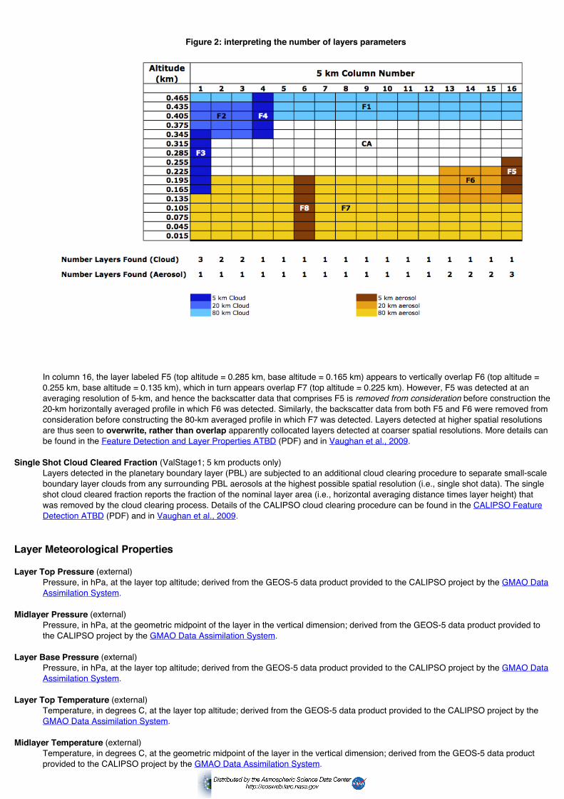
Figure 2: interpreting the number of layers parameters

In column 16, the layer labeled F5 (top altitude = 0.285 km, base altitude = 0.165 km) appears to vertically overlap F6 (top altitude =0.255 km, base altitude = 0.135 km), which in turn appears overlap F7 (top altitude = 0.225 km). However, F5 was detected at anaveraging resolution of 5-km, and hence the backscatter data that comprises F5 is removed from consideration before construction the20-km horizontally averaged profile in which F6 was detected. Similarly, the backscatter data from both F5 and F6 were removed fromconsideration before constructing the 80-km averaged profile in which F7 was detected. Layers detected at higher spatial resolutionsare thus seen to overwrite, rather than overlap apparently collocated layers detected at coarser spatial resolutions. More details canbe found in the Feature Detection and Layer Properties ATBD (PDF) and in Vaughan et al., 2009.

Single Shot Cloud Cleared Fraction (ValStage1; 5 km products only)Layers detected in the planetary boundary layer (PBL) are subjected to an additional cloud clearing procedure to separate small-scaleboundary layer clouds from any surrounding PBL aerosols at the highest possible spatial resolution (i.e., single shot data). The singleshot cloud cleared fraction reports the fraction of the nominal layer area (i.e., horizontal averaging distance times layer height) thatwas removed by the cloud clearing process. Details of the CALIPSO cloud clearing procedure can be found in the CALIPSO FeatureDetection ATBD (PDF) and in Vaughan et al., 2009.

Layer Meteorological Properties

Layer Top Pressure (external)Pressure, in hPa, at the layer top altitude; derived from the GEOS-5 data product provided to the CALIPSO project by the GMAO DataAssimilation System.

Midlayer Pressure (external)Pressure, in hPa, at the geometric midpoint of the layer in the vertical dimension; derived from the GEOS-5 data product provided tothe CALIPSO project by the GMAO Data Assimilation System.

Layer Base Pressure (external)Pressure, in hPa, at the layer top altitude; derived from the GEOS-5 data product provided to the CALIPSO project by the GMAO DataAssimilation System.

Layer Top Temperature (external)Temperature, in degrees C, at the layer top altitude; derived from the GEOS-5 data product provided to the CALIPSO project by the GMAO Data Assimilation System.

Midlayer Temperature (external)Temperature, in degrees C, at the geometric midpoint of the layer in the vertical dimension; derived from the GEOS-5 data productprovided to the CALIPSO project by the GMAO Data Assimilation System.

Layer Base Temperature (external)Temperature, in degrees C, at the layer base altitude; derived from the GEOS-5 data product provided to the CALIPSO project by the GMAO Data Assimilation System.

Relative Humidity (external; 5 km aerosol products only)Relative humidity, in percent, at the geometric midpoint of the layer in the vertical dimension; derived from the GEOS-5 data productprovided to the CALIPSO project by the GMAO Data Assimilation System.

Layer Measured Optical Properties

Integrated Attenuated Backscatter 532 (provisional @ 5 km; ValStage1 @ 1 km & 1/3 km)The 532 nm integrated attenuated backscatter (hereafter, γ'532 or IAB) for any layer is computed according to equation 3.14 in section3.2.9.1 of the CALIPSO Feature Detection ATBD (PDF).

For the uppermost layer in any column, the quality of the estimate for γ'532 is determined by the accuracy of the top and baseidentification, the reliability of the 532 nm channel calibrations, and by the signal-to-noise ratio (SNR) of the backscatter data within thelayer. For layers beneath the uppermost, the quality of our estimate for γ'532 also depends on either obtaining an independent estimateof the two-way transmittance, T2, for all overlying layers, or by estimating this quantity directly from the lidar backscatter data. In thosesituations where an extended region of clear air exists between successive layers, and where the uppermost layer has no more than amoderate optical depth of -- say -- between 0.4 and 2.0, T2 can be estimated directly from the attenuated backscatter data (albeit withsome uncertainty due to noise and the possibility of aerosol contamination of the clear air regions). Otherwise, the only way toestimate T2 is to compute a full extinction retrieval for the profile being examined. In this case, additional error can be introduced intothe estimate of γ'532 by uncertainties in the approximation of the lidar ratio(s) for the overlying layer(s). Furthermore, the effects oferrors caused by misestimating T2 can increase sharply as the optical thickness above a layer increases. For the 5 km layer products,the CALIOP processing scheme always attempts to correct estimates of γ'532 for the attenuation imparted by previously identifiedoverlying features. As a consequence, we will occasionally report unrealistically large values for γ'532 in the 5 km layer products.However, because extinction solutions are only derived for data averaged to a 5-km (or greater) resolution, the γ'532 values reported inthe 1 km and 1/3 km layer products are not corrected for the signal attenuation effects imparted by overlying layers.

The values reported for γ'532 should always be positive, and for the results derived directly from the layer detection algorithm (i.e., inthe 1 km and 1/3 km layer products) this is indeed always true. However, in the 5 km products there are certain rare and pathologicalcases where a secondary layer could only be detected after averaging to 20 km or even 80 km horizontally, and where the overlyinglayers were detected at 5 km and have vastly different optical depths. In these cases, integrating the reaveraged data within thesecondary layer will occasionally yield a negative γ'532. Such layers can be identified by a special CAD score of 105. All measured andderived optical properties for these layers are unreliable, and should be ignored. In evaluating the reliability of the spatial properties ofthese layers, users should carefully consider the layer IAB QA factor.

Integrated Attenuated Backscatter Uncertainty 532 (provisional @ 5 km; ValStage1 @ 1 km & 1/3 km)The uncertainties reported for the 532 nm integrated attenuated backscatters provide an estimate of the random error in thebackscatter signal. The general procedure used for calculating uncertainties for integrated quantities is described by Liu et al., 2006(PDF). The specific formula is given by equation 6.7 in the CALIPSO Feature Detection ATBD (PDF).

Attenuated Backscatter Statistics 532 (provisional @ 5 km; ValStage1 @ 1 km & 1/3 km)This field reports the minimum, maximum, mean, standard deviation, centroid, and skewness coefficient of the 532 nm attenuatedbackscatter coefficients for each layer. Formulas used for each of the statistical calculations can be found in section 6 of the CALIPSOFeature Detection ATBD (PDF).

Integrated Attenuated Backscatter 1064 (provisional @ 5 km; ValStage1 @ 1 km & 1/3 km)The 1064 nm integrated attenuated backscatter (hereafter, γ'1064) for any layer is computed according to equation 6.6 in section 6.5 ofthe CALIPSO Feature Detection ATBD (PDF).

As is the case for γ'532, in the uppermost layer within any column, the quality of the estimate for γ'1064 is determined by the accuracy ofthe top and base identification, the reliability of the 1064 nm calibration constant, and by the signal-to-noise ratio (SNR) of thebackscatter data within the layer. However, unlike the measurements at 532 nm, reliable estimates of T2 cannot be derived from ananalysis of the 1064 nm backscatter signal in the (assumed to be) clear air regions, and thus in the 5 km products, the T2 correctionsfor the attenuation from overlying layers are always obtained from an extinction solution that uses prescribed values of the lidar ratiosfor all overlying layers. As is the case at 532 nm, no T2 corrections are applied to the γ'1064 values reported in the 1 km and 1/3 kmlayer products. Furthermore, because the CALIOP layer detection algorithm typically examines only the 532 nm backscatter signals,negative (i.e., non-physical) values may occasionally be reported for γ'1064 in all resolutions of the layer products. Unlike the layers forwhich γ'532 is negative, layers with negative γ'1064 are not indicated by a special CAD score. Negative values of γ'1064 occur most oftenfor very weakly scattering layers (e.g., subvisible cirrus and faint aerosols) and in those layers for which the backscatter signal hasbeen highly attenuated by other, overlying layers.

Integrated Attenuated Backscatter Uncertainty 1064 (provisional @ 5 km; ValStage1 @ 1 km & 1/3 km)The uncertainties reported for the 1064 nm integrated attenuated backscatter values provide an estimate of the random error in thebackscatter signal. The general procedure used for calculating uncertainties for integrated quantities is described by Liu et al., 2006(PDF). The specific formula is given by equation 6.7 in the CALIPSO Feature Detection ATBD (PDF).

Attenuated Backscatter Statistics 1064 (provisional @ 5 km; ValStage1 @ 1 km & 1/3 km)This field reports the minimum, maximum, mean, standard deviation, centroid, and skewness coefficient of the 1064 nm attenuatedbackscatter coefficients for each layer. Formulas used for each of the statistical calculations can be found in section 6 of the CALIPSOFeature Detection ATBD (PDF).

Integrated Volume Depolarization Ratio (ValStage1)The layer integrated 532 nm volume depolarization ratio (hereafter, δv) is computed according to equation 6.10 in section 6.7 of the CALIPSO Feature Detection ATBD (PDF).

The quality of the estimate for δv is determined by the accuracy of the top and base identification, the reliability of the polarization gainratio calibration, and by the signal-to-noise ratio (SNR) of the backscatter data within the layer. In general, the CALIOP δv estimatesare highly reliable. Histograms of δv compiled for midlatitude cirrus in the northern hemisphere compare very well with previouslyreported distributions, e.g., Sassen & Benson, 2001 (PDF).

Integrated Volume Depolarization Ratio Uncertainty (ValStage1)The uncertainties reported for the 532 nm layer-integrated volume depolarization ratios provide an estimate of the total random error inthe combined backscatter signals (i.e., the 532 nm parallel and perpendicular signals within the feature). The general procedure usedfor calculating uncertainties for integrated quantities is described by Liu et al., 2006 (PDF). The specific formula is given by equation6.11 in the CALIPSO Feature Detection ATBD (PDF).

Volume Depolarization Ratio Statistics (ValStage1)This field reports the minimum, maximum, mean, standard deviation, centroid, and skewness coefficient of the 532 nm volumedepolarization ratios for each layer. Formulas used for each of the statistical calculations can be found in section 6 of the CALIPSOFeature Detection ATBD (PDF).

In regions with acceptable SNR, the accuracy with which the range resolved depolarization ratios can be determined will dependalmost entirely on the accuracy of the polarization gain ratio calibration.

Users can have high confidence in the calculation of all of the values in the depolarization ratio statistics fields. However, the meaningof these numbers can be somewhat obscure. This is because each of the range resolved depolarization ratios within any layer is theratio of two noisy numbers. Especially where the feature is relatively faint, and in regions of low SNR, data values in both thenumerator (the 532 nm perpendicular channel) and the denominator (the 532 nm parallel channel) can randomly and independentlyapproach zero, which in turn can generate extremely large or extremely small (and even non-physical) depolarization ratios. Whencomputing layer means, standard deviations, and centroids, these values can dominate the calculation, and thus return entirelyunrealistic estimates. When assessing the depolarization ratio that characterizes a layer, δv and the layer median are both morereliable indicators than the mean.

Integrated Attenuated Total Color Ratio (provisional @ 5 km; ValStage1 @ 1 km & 1/3 km)The layer integrated attenuated total color ratio (hereafter, χ'layer) is computed according to equation 6.13 in section 6.7 of the CALIPSO Feature Detection ATBD (PDF).

The quality of the estimate for χ'layer is determined by the accuracy of the top and base identification, the reliability of the 532 nmcalibration constant and the 1064 nm calibration constant, and by the signal-to-noise ratio (SNR) of the backscatter data within thelayer. For the 5 km layer products, the attenuated backscatter coefficients used in the calculation of χ'layer are corrected for theestimated overlying two-way transmittance. No such correction is attempted for the 1 km and 1/3 km values, as no extinction solutionis computed at these resolutions.

Integrated Attenuated Total Color Ratio Uncertainty (provisional @ 5 km; ValStage1 @ 1 km & 1/3 km)The uncertainties reported for the layer-integrated attenuated total color ratios provide an estimate of the total random error in thecombined backscatter signals (i.e., at 532 nm and 1064 nm). The general procedure used for calculating uncertainties for integratedquantities is described by Liu et al., 2006 (PDF). The specific formula is given by equation 6.14 in the CALIPSO Feature DetectionATBD (PDF).

Attenuated Total Color Ratio Statistics (provisional @ 5 km; ValStage1 @ 1 km & 1/3 km)This field reports the minimum, maximum, mean, standard deviation, centroid, and skewness coefficient of the attenuated total colorratios for each layer. Formulas used for each of the statistical calculations can be found in section 6 of the CALIPSO FeatureDetection ATBD (PDF).

Users can have high confidence in the calculation of all of the values in the attenuated total color ratio statistics fields. However, aswith the 532 nm depolarization ratio statistics, the meaning of the various numbers can be somewhat misleading. Like thedepolarization ratios, the attenuated total color ratios are produced by dividing one noisy number (the 1064 nm attenuated backscattercoefficient) by a second noisy number (the 532 nm attenuated backscatter coefficient). Depending on the noise in any pair of samples,the resulting values can range from large negative values to extremely large positive values. When computing layer means, standarddeviations, and centroids, these outliers can dominate the calculation, and thus return entirely unrealistic estimates.

Measured Two Way Transmittance 532 (provisional; 5 km products only)Provides the measured value of the layer two-way transmittance (T2) for isolated transparent layers. In this context, an isolated layer isone that is not in contact with another layer or the surface at either its upper or lower boundaries. T2 is derived by computing the ratioof the mean attenuated scattering ratios in the "clear air" regions immediately below and above the layer. Details of the calculation areprovided in the layer detection ATBD (PDF). This quantity is reported only for the 532 nm data, as the CALIOP 1064 nm channel is

essentially insensitive to molecular backscatter. Physically meaningful measurements of two-way transmittance lie between 0 and 1;however, due to noise in the backscatter signal, and perhaps to undetected aerosol contamination of the "clear air" regions, the valuesreported in the CALIOP data products will sometimes exceed these bounds.

Measured Two Way Transmittance Uncertainty 532 (provisional; 5 km products only)The relative error in the two-way transmittance measurement, calculated using standard techniques for error propagation in ratioedquantities.

Opacity Flag (ValStage1; 5 km products only)In the context of the 5-km CALIOP layer products, a layer is considered opaque if (a) it is the lowest feature detected in a column, and(b) it is not subsequently classified as a surface return. An opacity flag value of 1 indicates an opaque layer; values of 0 indicatetransparent layers. Users should be aware that the opacity flag does not indicate that an individual layer is actually opaque in thenormal sense of the term. Instead, the opacity flag identifies that layer in which the backscatter signal becomes completely attenuated(i.e., indistinguishable from the background signal level). For those features having an opacity flag of 1, the reported base altitudemust be considered as an apparent base, rather than a true base.

Because all features reported in 1/3-km and 1-km layer products are detected at a single horizontal averaging resolution (i.e., either at1/3-km or 1-km), the opacity flag is not reported. When using these products, opacity, in the sense described above, can be assessedas follows. If the surface was detected (i.e., the lidar surface altitude field does not contain fill values) then there are no opaque layersin the column. If the surface was not detected, then the lowest layer in the column is considered to be opaque.

Layer Derived Optical Properties

Feature Optical Depth 532 (provisional; 5 km products only)Feature Optical Depth 1064 (provisional; 5 km aerosol products only)

Reports estimates of layer optical depth computed according to the procedures outlined in the CALIOP extinction retrieval ATBD(PDF). Estimates for aerosol optical depths are provided at both wavelengths. Because the extinction coefficients for clouds arelargely independent of wavelength in the spectral region sampled by CALIOP, cloud optical depth is reported only for the 532 nmmeasurements. When using any of these values in scientific studies, users are cautioned to take note of several important caveats:

For the vast majority of cases, CALIOP cannot provide a direct measurement of layer optical depth. In these cases, estimatesof optical depth are derived using extinction-to-backscatter ratios (i.e., lidar ratios) that are specified based on an assessmentof layer type and subtype. Uncertainties in the value of the lidar ratio, which can arise both from natural variability and fromoccasional misclassification of layer type, propagate non-linearly into subsequent estimates of layer optical depth.

Retrievals of optical depth from space-based lidar measurements must account for contributions from multiple scattering thatare generally considered negligible in ground-based and aircraft based measurements. The theoretical basis for CALIPSO'streatment of multiple scattering is provided in the extinction retrieval ATBD (PDF) and in Winker, 2003 (PDF).

Similar to the layer detection problem, estimates of layer optical depth become increasingly fraught with error in multiple layerscenes, as errors incurred in overlying layers are propagated into the solutions derived for underlying features.

IMPORTANT NOTICE: before proceeding, all users of the CALIOP optical depth data should read and thoroughly understandthe information provided in the Profile Products Data Quality Summary. This summary contains an expanded description of theextinction retrieval process from which the layer optical depths are derived, and provides essential guidance in the appropriateuse of all CALIOP extinction-related data products.

Despite these caveats, users should not be unduly pessimistic about the quality and usability of the CALIPSO optical depth estimates.Figure 3 (below) shows a preliminary comparison of CALIPSO version 3 aerosol optical depths with the optical depths derived fromMODIS for all daytime measurements acquired during January 2007. The comparison is generally good, with MODIS appearing toslightly over-estimate values at the lower end of the optical depth range.

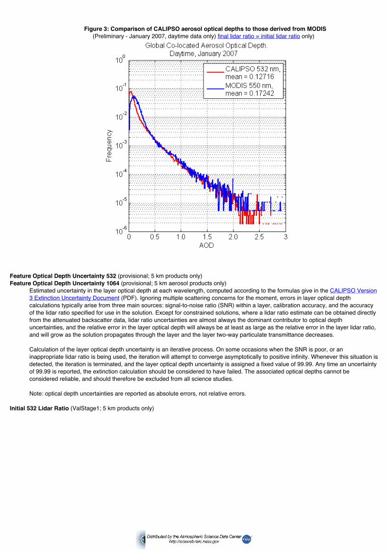
Figure 3: Comparison of CALIPSO aerosol optical depths to those derived from MODIS(Preliminary - January 2007, daytime data only) final lidar ratio = initial lidar ratio only)

Feature Optical Depth Uncertainty 532 (provisional; 5 km products only)Feature Optical Depth Uncertainty 1064 (provisional; 5 km aerosol products only)

Estimated uncertainty in the layer optical depth at each wavelength, computed according to the formulas give in the CALIPSO Version3 Extinction Uncertainty Document (PDF). Ignoring multiple scattering concerns for the moment, errors in layer optical depthcalculations typically arise from three main sources: signal-to-noise ratio (SNR) within a layer, calibration accuracy, and the accuracyof the lidar ratio specified for use in the solution. Except for constrained solutions, where a lidar ratio estimate can be obtained directlyfrom the attenuated backscatter data, lidar ratio uncertainties are almost always the dominant contributor to optical depthuncertainties, and the relative error in the layer optical depth will always be at least as large as the relative error in the layer lidar ratio,and will grow as the solution propagates through the layer and the layer two-way particulate transmittance decreases.

Calculation of the layer optical depth uncertainty is an iterative process. On some occasions when the SNR is poor, or aninappropriate lidar ratio is being used, the iteration will attempt to converge asymptotically to positive infinity. Whenever this situation isdetected, the iteration is terminated, and the layer optical depth uncertainty is assigned a fixed value of 99.99. Any time an uncertaintyof 99.99 is reported, the extinction calculation should be considered to have failed. The associated optical depths cannot beconsidered reliable, and should therefore be excluded from all science studies.

Note: optical depth uncertainties are reported as absolute errors, not relative errors.

Initial 532 Lidar Ratio (ValStage1; 5 km products only)

Initial 1064 Lidar Ratio (ValStage1; 5 km aerosol products only)Retrieving optical depth and profiles of extinction and backscatter coefficients from the CALIOP measurements requires an estimate ofthe particulate extinction-to-backscatter ratio, which in the lidar community is commonly known as the "lidar ratio". These initialestimates are selected based on the type and subtype of the layer being analyzed. The values used in the current release are givenbelow. Values highlighted in red have been changed since the version 2 release.

Initial lidar ratios used in the version 3.01 extinction solver Type Subtype Initial 532 nm lidar ratio Initial 1064 nm lidar ratiocloud water 19 ± 10 sr N/Acloud ice 25 ± 10 sr N/Acloud unknown phase 22 ± 11 sr N/A

aerosol marine 20 ± 6 sr 45 ± 23 sraerosol desert dust 40 ± 20 sr 55 ± 17 sraerosol polluted continental 70 ± 25 sr 30 ± 14 sraerosol clean continental 35 ± 16 sr 30 ± 17 sraerosol polluted dust 55 ± 22 sr 48 ± 24 sraerosol biomass burning 70 ± 28 sr 40 ± 24 sr

stratospheric all 25 ± 10 sr 25 ± 10 sr

The aerosol lidar ratios used for the CALIOP analyses represent well established mean values that are characteristic of the naturalvariability exhibited for each aerosol species (e.g., see Omar et al., 2005 (PDF); Cattrall et. al., 2005; and Figure 4 below). The clearimplication of this natural variability is that even for those cases where the aerosol type is correctly identified, the initial lidar ratiorepresents an imperfect estimate of the layer-effective lidar ratio of any specific aerosol layer. These same caveats apply equally tothe mean values used for the initial cloud lidar ratios. For all layer types, cloud-aerosol discrimination errors can exacerbate the errorassociated with the specification of the initial lidar ratio. Uncertainty can also be introduced by the cloud ice-water phase classificationand the aerosol subtype identification procedures. However, the CALIOP extinction algorithm incorporates some error-correctingmechanisms that in many cases will adjust the initial estimate of lidar ratio so that a more suitable value is ultimately used in theretrieval. Details of the lidar ratio adjustment scheme are provided in the extinction retrieval ATBD (PDF). Algorithm architecturalinformation and generalized error analyses for CALIPSO's cloud-aerosol discrimination algorithms, cloud ice-water phase algorithms,and aerosol subtyping algorithms can be found in the CALIPSO Scene Classification ATBD (PDF).

Figure 4: Distributions for AERONET-derived lidar ratios, computed for aerosol types described in Omar et al., 2005 (PDF);

The version 3.0 aerosol subtyping scheme is different from the previous versions. Two of the aerosol models, dust and polluted dust,discussed in Omar et al. (2009) and used in prior versions have been updated in light of the latest advances in the science. Recentmeasurements of size distributions of dust aerosol during NAMMA and T-Matrix calculations of the phase functions allowed a morerealistic estimate of the dust lidar ratio at 1064 nm which, thus far, was based on a single measurement during SAFARI 2000. Thedust phase function (squares in Figure 4a) is determined by T-Matrix calculations using NAMMA measurements of size distributionsand refractive indices and the smoke phase functions (circles in Figure 4a) are determined from Mie calculations using sizedistributions and refractive indices of the biomass burning cluster of the AERONET measurements. The dust lidar ratios determinedpartly using NAMMA measurements are 40 sr and 55 sr at 532 nm and 1064 nm, respectively. The 55 sr at 1064 nm is a significantdeparture from the 30 sr used to calculate 1064 nm extinction coefficients in previous versions.

Since the polluted dust model is built from a smoke fine component and a dust coarse component, the above adjustment in the dustmodel is also reflected in the polluted dust model. A composite phase function (Figure 5b) of dust coarse mode and smoke fine modefrom the individual phase functions is shown in Figure 5a. The resulting polluted dust lidar ratios are 55 sr at 532 nm and 48 sr at 1064nm. The former is a departure from the old values of 65 sr at 532 nm. This is because in the original model most of the polluted dustaerosol was comprised of smoke, while this new model, partly based on NAMMA observations, apportions a significant surface area tothe coarse mode dominated by dust. The old model used Mie calculations to generate polluted dust phase functions and lidar ratioswhile the new model uses Mie model calculations for the fine mode (smoke) and T-Matrix calculations for the coarse mode (dust) togenerate the phase functions and lidar ratios.

Figure 5: (a) Smoke and Dust phase functions determined by Mie and T-Matrix calculations respectively, and (b) compositedust and smoke phase functions representative of the polluted dust aerosol model

Final 532 Lidar Ratio (provisional; 5 km products only)Final 1064 Lidar Ratio (provisional; 5 km aerosol products only)

This parameter reports the lidar ratio in use at the conclusion of the extinction processing for each layer. The final lidar ratio may be (1)the initial lidar ratio supplied by the Scene Classification Algorithms, (2) the result of modifications to this initial lidar ratio to avoid a non-physical solution, or (3) a lidar ratio determined from a measured layer transmittance. In cases where a suitable estimate of layeroptical depth is available, the lidar ratio derived from that measurement will be used to generate the extinction solution. The extinctionprocessing terminates when either a successful solution is obtained, or when the required adjustments to the lidar ratio exceed somepredetermined bounds. Within those bounds, which range from 0 sr to 250 sr in the version 3.01 release, the extinction algorithm will,if necessary, adjust the initial lidar ratio as required to produce a physically plausible solution consistent with the measured data. Userscan determine the status of the final lidar ratio by examining the extinction QC flags.

For weakly scattering features, the lidar ratio is most often left unchanged by the extinction solver, as a physical solution is usuallyobtained on the first iteration. In these cases, the uncertainties in the final lidar ratio are the same as the uncertainties in the initial lidarratio. The exception to this statement would be if either the cloud-aerosol discrimination or the layer sub-typing procedures havemisclassified the layer. However, for weak layers, the relative error in the lidar ratio is (approximately) linearly related to the resultingerror in the derived optical depth estimate.

Retrievals of opaque and strongly scattering layers are very sensitive to the initial lidar ratio selection. Too large a value will cause theretrieval algorithm to, in effect, extinguish all available signal before reaching the measured base of the feature. When that point isreached the retrieval becomes numerically unstable and the calculated extinction coefficients will asymptote toward positive infinity. Inthese cases, a successful solution can only be obtained by reducing the lidar ratio. The CALIOP extinction routine does thisautomatically, and will repeat the process until a stable solution is achieved. When this happens, the final lidar ratio reported in thedata products is the first one for which a physically meaningful (albeit not necessarily correct) solution was obtained for the entiremeasured depth of the layer.

The optical depths and extinction profiles derived in those cases where the layer lidar ratio must be reduced are generally notaccurate. The current lidar ratio reduction scheme terminates after identifying (a very close estimate of) the largest lidar ratio for whicha physically meaningful solution can be generated for the backscatter measured in the layer. However, the optical depths and

extinction profiles reported in these situations can only be considered as upper bounds; the true values are somewhat, or perhapseven significantly, lower. Because the associated optical depth uncertainties cannot be reasonably estimated, these data should beexcluded from statistical analyses of layer optical properties, and even the most sophisticated users are advised to treat these caseswith extreme caution.

When an independent estimate of layer optical depth is available from a measured layer two-way transmittance, the CALIOP extinctionalgorithm will retrieve the optimal estimate of the layer-effective lidar ratio, irrespective of layer type, and use this retrieved lidar ratio inthe extinction retrieval. These so-called 'constrained' retrievals are more accurate than unconstrained retrievals. For constrainedretrievals, the uncertainty in the final lidar ratio can be well estimated using equation 7.4 from the CALIPSO Scene ClassificationATBD (PDF). An extinction QC value of 1 indicates a successful constrained retrieval.

Lidar Ratio 532 Selection Method (external; 5 km products only)Lidar Ratio 1064 Selection Method (external; 5 km aerosol products only)

Specifies the internal procedure used to select the initial lidar ratio for each layer; valid values in this field are...

Value Method0 not determined1 constrained retrieval (using two-way transmittance)2 based on cloud phase3 based on aerosol species99 fill value

Layer Effective 532 Multiple Scattering Factor (provisional; 5 km aerosol products only)Layer Effective 1064 Multiple Scattering Factor (provisional; 5 km products only)

The layer effective multiple scattering factors, η532 and η1064, are specified at each wavelength according to layer type and subtype.Values range between 0 and 1; 1 corresponds to the limit of single scattering only, with smaller values indicating increasingcontributions to the backscatter signal from multiple scattering. Multiple scattering effects are different in aerosols, ice clouds, andwater clouds. A discussion of multiple scattering factors for ice clouds and several aerosol types can be found in Winker, 2003 (PDF).Multiple scattering in water clouds is discussed in Winker and Poole (1995).

Ice clouds: for the CALIOP viewing geometry, simulations show multiple scattering effects are nearly independent of range and, asparameterized in the CALIOP retrieval algorithm (Winker et al. 2009), are nearly independent of extinction. In Version 2, ice cloudswere assigned a range-independent multiple scattering factor of η532 = 0.6. Validation comparisons indicate this is an appropriatevalue and the same value is used in Version 3.

Water clouds: in Version 2 the multiple scattering factor for water clouds was set to unity, resulting in large errors in retrievals ofextinction and optical depth. In Version 3, a value of η532 = 0.6 is used. Based on Monte Carlo simulations of multiple scattering, thisvalue appears to be appropriate for semitransparent water clouds (τ < 1). (It is purely coincidental this is the same value used for iceclouds.) For denser water clouds (τ > 1) the multiply-scattered component of the signal becomes much larger than the single-scatteredcomponent, η532 becomes dependent on both cloud extinction and range into the cloud, and the retrieval becomes very sensitive toerrors in the multiple scattering factor used. In these cases the multiple scattering cannot be properly accounted for in the currentretrieval algorithm and retrieval results are unreliable.

Aerosols: simulations of multiple scattering effects on retrievals of aerosol layer optical depth indicate the effects are small in mostcases. There is uncertainty in these estimates, however, due to poor knowledge of aerosol scattering phase functions. Validationcomparisons conducted to date do not indicate significant multiple scattering effects on aerosol extinction profile retrievals. Multiplescattering effects may become significant in dense aerosol layers (σ > 1 /km), but in these cases retrieval errors are usually dominatedby uncertainties in the lidar ratio or failure to fully penetrate the layer. In Version 3, as in Version 2, multiple scattering factors for bothwavelengths are set to unity.

Integrated Particulate Depolarization Ratio (provisional; 5 km products only)Similar to the layer-integrated volume depolarization ratio, except for particulates only. The particulate depolarization ratio representsthe contribution to the volume depolarization ratio that is due only to the cloud and/or aerosol particles within the layer. For non-spherical particles (e.g., ice, dust) the particulate depolarization ratio will normally be higher than the volume depolarization ratio (howmuch higher depends on the particulate concentration within the volume). For layers consisting of spherical particles, the particulatedepolarization ratio would normally be equal to or even slightly lower than the volume depolarization ratios. However, if the layeroptical depth is high (e.g., water clouds), multiple scattering can cause the integrated particulate depolarization ratio to be substantiallyhigher than otherwise expected.

While the volume depolarization ratio is a direct measurement, the layer integrated 532 nm particulate depolarization ratio, δp, is a post-extinction quantity, calculated from ratio of the layer integrated perpendicular and parallel polarization components of particulatebackscatter coefficient within the layer, using

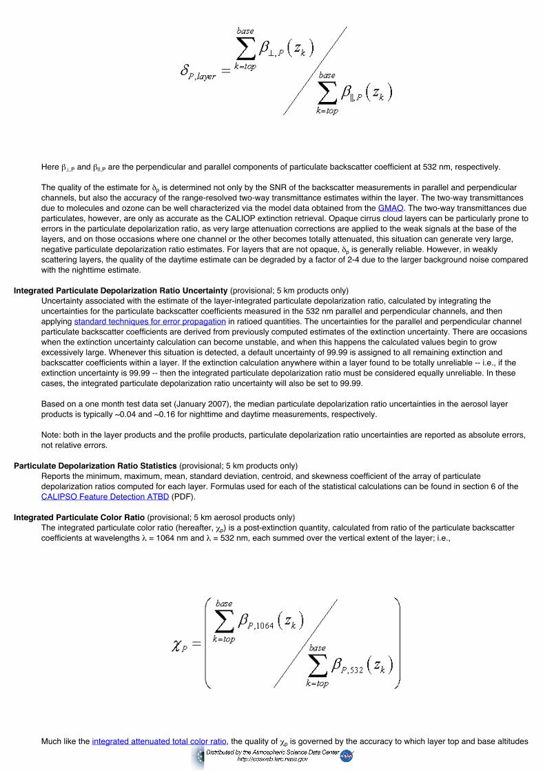
Here β⊥,P and β||,P are the perpendicular and parallel components of particulate backscatter coefficient at 532 nm, respectively.

The quality of the estimate for δp is determined not only by the SNR of the backscatter measurements in parallel and perpendicularchannels, but also the accuracy of the range-resolved two-way transmittance estimates within the layer. The two-way transmittancesdue to molecules and ozone can be well characterized via the model data obtained from the GMAO. The two-way transmittances dueparticulates, however, are only as accurate as the CALIOP extinction retrieval. Opaque cirrus cloud layers can be particularly prone toerrors in the particulate depolarization ratio, as very large attenuation corrections are applied to the weak signals at the base of thelayers, and on those occasions where one channel or the other becomes totally attenuated, this situation can generate very large,negative particulate depolarization ratio estimates. For layers that are not opaque, δp is generally reliable. However, in weaklyscattering layers, the quality of the daytime estimate can be degraded by a factor of 2-4 due to the larger background noise comparedwith the nighttime estimate.

Integrated Particulate Depolarization Ratio Uncertainty (provisional; 5 km products only)Uncertainty associated with the estimate of the layer-integrated particulate depolarization ratio, calculated by integrating theuncertainties for the particulate backscatter coefficients measured in the 532 nm parallel and perpendicular channels, and thenapplying standard techniques for error propagation in ratioed quantities. The uncertainties for the parallel and perpendicular channelparticulate backscatter coefficients are derived from previously computed estimates of the extinction uncertainty. There are occasionswhen the extinction uncertainty calculation can become unstable, and when this happens the calculated values begin to growexcessively large. Whenever this situation is detected, a default uncertainty of 99.99 is assigned to all remaining extinction andbackscatter coefficients within a layer. If the extinction calculation anywhere within a layer found to be totally unreliable -- i.e., if theextinction uncertainty is 99.99 -- then the integrated particulate depolarization ratio must be considered equally unreliable. In thesecases, the integrated particulate depolarization ratio uncertainty will also be set to 99.99.

Based on a one month test data set (January 2007), the median particulate depolarization ratio uncertainties in the aerosol layerproducts is typically ~0.04 and ~0.16 for nighttime and daytime measurements, respectively.

Note: both in the layer products and the profile products, particulate depolarization ratio uncertainties are reported as absolute errors,not relative errors.

Particulate Depolarization Ratio Statistics (provisional; 5 km products only)Reports the minimum, maximum, mean, standard deviation, centroid, and skewness coefficient of the array of particulatedepolarization ratios computed for each layer. Formulas used for each of the statistical calculations can be found in section 6 of the CALIPSO Feature Detection ATBD (PDF).

Integrated Particulate Color Ratio (provisional; 5 km aerosol products only)The integrated particulate color ratio (hereafter, χp) is a post-extinction quantity, calculated from ratio of the particulate backscattercoefficients at wavelengths λ = 1064 nm and λ = 532 nm, each summed over the vertical extent of the layer; i.e.,

Much like the integrated attenuated total color ratio, the quality of χp is governed by the accuracy to which layer top and base altitudes

are determined and by the signal-to-noise ratios of the backscatter data within the layer. Additionally, since all of the βP,λ(z) values arederived by the Hybrid Extinction Retrieval Algorithm (HERA), the quality of χp also depends on the success of the HERA profile solverin deriving accurate solutions for βP,λ(z). As such, the quality of χp can be partially assessed via the extinction QC flags which reportthe final state of the HERA solution attempt. In general, solutions where the final lidar ratio is unchanged (extinction QC = 0) or theextinction solution is constrained (extinction QC = 1) yield physically plausible solutions more often. Conversely, solutions tend to bemore uncertain in those cases where the lidar ratio for either wavelength must be reduced.

Integrated Particulate Color Ratio Uncertainty (provisional; 5 km aerosol products only)Uncertainty associated with the estimate of the layer-integrated particulate backscatter color ratio, calculated by first integrating theuncertainties for the particulate backscatter coefficients measured at each wavelength, and then applying standard techniques forerror propagation in ratioed quantities. The error estimates in the particulate backscatter coefficients at both wavelengths arecomputed by the extinction retrieval algorithm. There are occasions when this calculation can become unstable, and the backscatteruncertainty calculation can grow excessively large. In these cases, a default uncertainty of 99.99 is assigned to all remainingbackscatter coefficients (and extinction) coefficients within a layer. If the backscatter uncertainty calculation fails anywhere within alayer -- that is, if the uncertainty in any of the backscatter coefficients used to compute the particulate color ratio uncertainty is set to99.99 -- then the particulate color ratio uncertainty for that layer will also be reported as 99.99.

Note: Uncertainties for layer-integrated particulate backscatter color ratios are reported as absolute errors, not relative errors.

Particulate Color Ratio Statistics (provisional; 5 km aerosol products only)Reports the minimum, maximum, mean, standard deviation, centroid, and skewness coefficient of the array of particulate backscattercolor ratios computed for each layer. Formulas used for each of the statistical calculations can be found in section 6 of the CALIPSOFeature Detection ATBD (PDF).

Users can have high confidence in the calculation of all the values in the attenuated particulate color ratio statistics fields. However,particulate color ratios are produced by dividing one noisy number (the 1064 nm mean particulate backscatter coefficient) by a secondnoisy number (the 532 nm mean particulate backscatter coefficient), resulting in values that can range from large negative values toextremely large positive values, depending on the noise in any pair of samples. When computing layer means, standard deviations,and centroids, these outliers can dominate the calculation, and thus return entirely unrealistic estimates. Therefore, the integratedparticulate ratio characterizes the particulate color ratio of a layer more reliably than does the mean value of the individual particulatecolor ratios within a layer.

Ice Water Path (provisional; 5 km cloud products only)The integral, from layer top to layer base, of the ice-water content profile within any ice cloud layer. Ice water content is derived fromthe cloud particulate extinction coefficient using a parameterization derived from in-situ measurements (see Heymsfield, Winker, andvan Zadelhoff, Extinction-ice water content-effective radius algorithms for CALIPSO, GRL, vol. 32).

Ice Water Path Uncertainty (provisional; 5 km cloud products only)Uncertainty associated with the estimate of ice water path, computed by integrating the uncertainties computed for the ice watercontent within the layer. Because the ice water content is derived directly from the 532 nm extinction estimates, uncertainties in icewater path are directly related to uncertainties in layer optical depths. If the 532 nm optical depth for a layer is entirely uncertain (i.e., Δτ = 99.99), the ice water path uncertainty will also be entirely uncertain (i.e., ΔIWP = 99.99).

Cirrus Shape Parameter (5 km cloud products only)Not calculated for the current release; data products contain fill values in this field.

Cirrus Shape Parameter Invalid Points (5 km cloud products only)Not calculated for the current release; data products contain fill values in this field.

Cirrus Shape Parameter Uncertainty (5 km cloud products only)Not calculated for the current release; data products contain fill values in this field.

Layer QA Information

CAD Score (ValStage1)The cloud-aerosol discrimination (CAD) score, which is reported in the 1-km and 5-km layer products, provides a numerical confidencelevel for the classification of layers by the CALIOP cloud-aerosol discrimination algorithm. The CAD algorithm separates clouds andaerosols based on multi-dimensional histograms of scattering properties (e.g., intensity and spectral dependence) as a function ofgeophysical location. In areas where there is no overlap or intersection between these histograms, features can be classified withcomplete confidence (i.e., |CAD score| = 100).

In the current release (version 3), the CAD algorithm uses newly developed five-dimensional (5D) probability density functions (PDFs),rather than the three-dimensional (3D) PDFs used in previous versions. In addition to the parameters used in the earlier 3D version ofthe algorithm (layer mean attenuated backscatter at 532 nm, layer-integrated attenuated backscatter color ratio, and altitude), the new5D PDFs also include feature latitude and the layer-integrated volume depolarization ratio. Detailed descriptions of the CAD algorithmcan be found in Sections 4 and 5 of the CALIPSO Scene Classification ATBD (PDF). Enhancements made to incorporate the 5DPDFs used in version 3 release are described in Liu et al., 2010 (PDF). For further information on the CAD algorithm architecture and

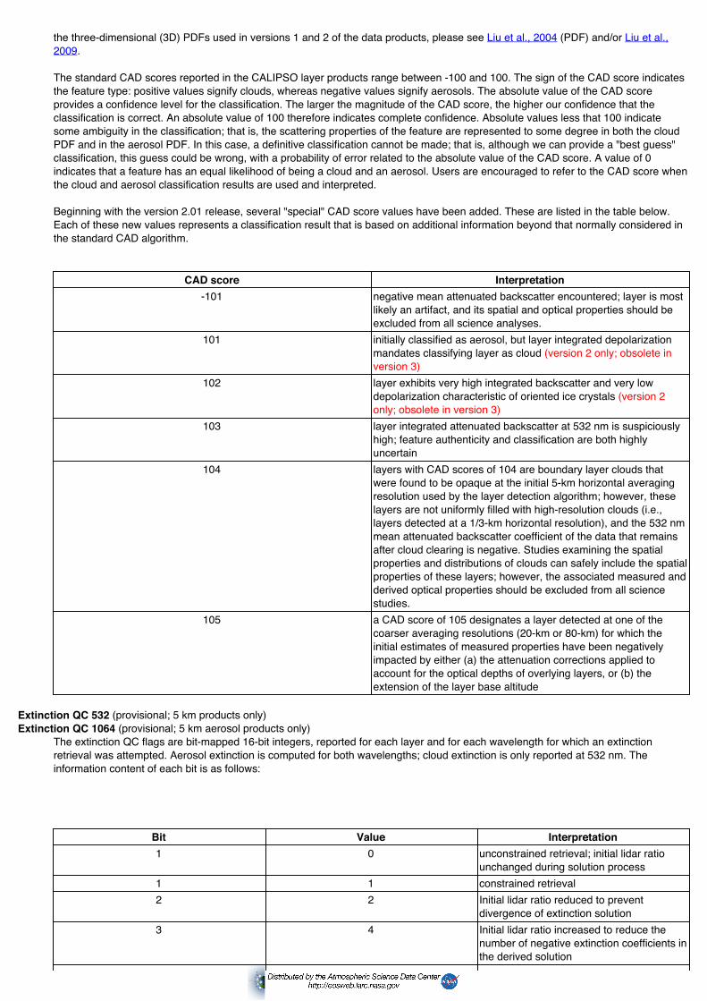
the three-dimensional (3D) PDFs used in versions 1 and 2 of the data products, please see Liu et al., 2004 (PDF) and/or Liu et al.,2009.

The standard CAD scores reported in the CALIPSO layer products range between -100 and 100. The sign of the CAD score indicatesthe feature type: positive values signify clouds, whereas negative values signify aerosols. The absolute value of the CAD scoreprovides a confidence level for the classification. The larger the magnitude of the CAD score, the higher our confidence that theclassification is correct. An absolute value of 100 therefore indicates complete confidence. Absolute values less that 100 indicatesome ambiguity in the classification; that is, the scattering properties of the feature are represented to some degree in both the cloudPDF and in the aerosol PDF. In this case, a definitive classification cannot be made; that is, although we can provide a "best guess"classification, this guess could be wrong, with a probability of error related to the absolute value of the CAD score. A value of 0indicates that a feature has an equal likelihood of being a cloud and an aerosol. Users are encouraged to refer to the CAD score whenthe cloud and aerosol classification results are used and interpreted.

Beginning with the version 2.01 release, several "special" CAD score values have been added. These are listed in the table below.Each of these new values represents a classification result that is based on additional information beyond that normally considered inthe standard CAD algorithm.

CAD score Interpretation-101 negative mean attenuated backscatter encountered; layer is most

likely an artifact, and its spatial and optical properties should beexcluded from all science analyses.

101 initially classified as aerosol, but layer integrated depolarizationmandates classifying layer as cloud (version 2 only; obsolete inversion 3)

102 layer exhibits very high integrated backscatter and very lowdepolarization characteristic of oriented ice crystals (version 2only; obsolete in version 3)

103 layer integrated attenuated backscatter at 532 nm is suspiciouslyhigh; feature authenticity and classification are both highlyuncertain

104 layers with CAD scores of 104 are boundary layer clouds thatwere found to be opaque at the initial 5-km horizontal averagingresolution used by the layer detection algorithm; however, theselayers are not uniformly filled with high-resolution clouds (i.e.,layers detected at a 1/3-km horizontal resolution), and the 532 nmmean attenuated backscatter coefficient of the data that remainsafter cloud clearing is negative. Studies examining the spatialproperties and distributions of clouds can safely include the spatialproperties of these layers; however, the associated measured andderived optical properties should be excluded from all sciencestudies.

105 a CAD score of 105 designates a layer detected at one of thecoarser averaging resolutions (20-km or 80-km) for which theinitial estimates of measured properties have been negativelyimpacted by either (a) the attenuation corrections applied toaccount for the optical depths of overlying layers, or (b) theextension of the layer base altitude

Extinction QC 532 (provisional; 5 km products only)Extinction QC 1064 (provisional; 5 km aerosol products only)

The extinction QC flags are bit-mapped 16-bit integers, reported for each layer and for each wavelength for which an extinctionretrieval was attempted. Aerosol extinction is computed for both wavelengths; cloud extinction is only reported at 532 nm. Theinformation content of each bit is as follows:

Bit Value Interpretation1 0 unconstrained retrieval; initial lidar ratio

unchanged during solution process1 1 constrained retrieval2 2 Initial lidar ratio reduced to prevent

divergence of extinction solution3 4 Initial lidar ratio increased to reduce the

number of negative extinction coefficients inthe derived solution

4 8 Calculated backscatter coefficient exceedsthe maximum allowable value

5 16 Layer being analyzed has been identified bythe feature finder as being totallyattenuating (i.e., opaque)

6 32 Estimated optical depth error exceeds themaximum allowable value

7 64 Solution converges, but with anunacceptably large number of negativevalues

8 128 Retrieval terminated at maximum iterations9 256 No solution possible within allowable lidar

ratio bounds16 32768 Fill value or no solution attempted

The bit assignments are additive, so that (for example) an extinction QC value of 18 represents an unconstrained retrieval (bit 1 isNOT set) for which the lidar ratio was reduced to prevent divergence (+2; bit 2 is set), and for which the feature finder has indicatedthat the layer is opaque (+16; bit 5 is set). For the version 2.01 release, bits 10-15 are not used. Complete information about theconditions under which each extinction QC bit is toggled can be found in the CALIPSO Extinction Retrieval ATBD (PDF).

Feature Classification Flags (ValStage1)For each layer, we report a set of feature classification flags that provide assessments of (a) feature type (e.g., cloud vs. aerosol vs.stratospheric layer); (b) feature subtype; (c) layer ice-water phase (clouds only); and (d) the amount of horizontal averaging requiredfor layer detection. The complete set of flags is stored as a single 16-bit integer. A comprehensive description of the feature finderclassification flags, including their derivation and physical significance, quality assessments, and guidelines for interpreting them incomputer codes, can be found in the documentation for the vertical feature mask data product.

Correct interpretation of the feature subtype bits depends on the status of the feature type; e.g., the interpretation is different for cloudsand aerosols. For aerosols, the feature subtype is one of eight types: desert dust, biomass burning, background, polluted continental,marine, polluted dust, other, and 'not determined'. Desert dust is mostly mineral soil. Biomass burning is an aged smoke aerosolconsisting primarily of soot and organic carbon (OC), clean continental (also referred to as background or rural aerosol) is a lightlyloaded aerosol consisting of sulfates (SO4

2-), nitrates (NO3-), OC, and Ammonium (NH4

+), polluted continental is background aerosolwith a substantial fraction of urban pollution, marine is a hygroscopic aerosol that consists primarily of sea-salt (NaCl), and polluteddust is a mixture of desert dust and smoke or urban pollution. Extensive test data generated prior to the version 3 release revealed anegligibly minute number of layers with spurious lidar ratios and aerosol type designations. These trace layers are currently labeled'not determined'. The 'other' designation is a place-holder for another, yet to be determined, aerosol type. While this set does not coverall possible aerosol mixing scenarios, it accounts for a majority of mesoscale aerosol layers. In essence the algorithm trades offcomplex transient multi-component mixtures for relatively stable layers with large horizontal extent (10-1000 km).

Layer Base ExtendedA non-zero value indicates that the base of the layer has been extended from the initial altitude assigned by the layer detectionalgorithm to a new, lower altitude lying three range bins (90 m) above the Earth's surface. Non-zero values represent the layer's feature classification flags prior to the base being extended.

In Version 1 and 2 data, the base altitudes of optically thick aerosol layers were sometimes biased high due to lidar signal attenuationor signal perturbations, causing aerosol optical depth (AOD) underestimates. In Version 3, to compensate for this, layer base altitudesof aerosol layers meeting the following criteria (hereafter termed, 'extended layers') are lowered to three range bins (90 m) from thesurface as reported by the lidar surface elevation. The criteria for aerosol layer base extension are:

1. The layer must be the lowest layer in the 5 km resolution column2. The surface must be detected below the layer3. The difference between the original base altitude and Lidar Surface Elevation must be less than the science-tunable

parameter, 'maximum gap distance', currently = 2.5 km4. The mean attenuated backscatter at 532 nm beneath the original base altitude must be positive

These criteria attempt to ensure that only boundary-layer aerosol layers with useable signals beneath their original bases areextended. The possibility of introducing surface contamination in layer optical properties is reduced by assigning the extended base toan altitude 90 m above the local surface height. Hence, surface contamination in extended layers is minimal and confined to regionswith rugged terrain. However, this also means that profiles within layers with extended bases always stop 90 meters above thesurface. In four months of global test data, the base altitudes of 8.6% of all layers originally classified as aerosol were extended, withaverage base altitudes lowered by 0.54 km.

Layer descriptors are re-computed after base extension and each extended layer is re-analyzed by the scene classification algorithmsto assign feature type, subtype, and CAD Score. Consequently, the feature type or subtype of these layers may change since theiroptical properties have changed. Hence, layer base extended descriptors are populated with the feature classification flags of theselayers prior to base extension so their previous type and subtype can be discerned. In four months of test data, 17% of extendedaerosol layer subtypes changed due to base extension. Additionally, 12% of all extended aerosol layers were reclassified as cloudlayers, accounting for 0.3% of all cloud layers. This typically occurs in scenes with low SNR, or when surface contamination is

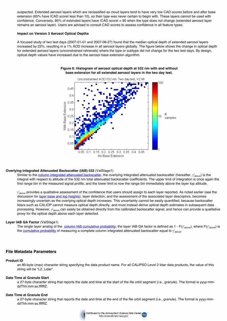
suspected. Extended aerosol layers which are reclassified as cloud layers tend to have very low CAD scores before and after baseextension (65% have |CAD score| less than 10), so their type was never certain to begin with. These layers cannot be used withconfidence. Conversely, 85% of extended layers have |CAD score| > 90 when the type does not change (extended aerosol layerremains an aerosol layer). Users are advised to consult CAD scores to assess confidence in all feature types.

Impact on Version 3 Aerosol Optical Depths

A focused study of two test days (2007-01-01 and 2007-08-27) found that the median optical depth of extended aerosol layersincreased by 22%, resulting in a 1% AOD increase in all aerosol layers globally. The figure below shows the change in optical depthfor extended aerosol layers (unconstrained retrievals) where the type or subtype did not change for the two test days. By design,optical depth values have increased due to the aerosol base extension algorithm.

Figure 6: Histogram of aerosol optical depth at 532 nm with and withoutbase extension for all extended aerosol layers in the two day test.

Overlying Integrated Attenuated Backscatter (IAB) 532 (ValStage1)Similar to the column integrated attenuated backscatter, the overlying integrated attenuated backscatter (hereafter, γ'above) is theintegral with respect to altitude of the 532 nm total attenuated backscatter coefficients. The upper limit of integration is once again thefirst range bin in the measured signal profile, and the lower limit is now the range bin immediately above the layer top altitude.

γ'above provides a qualitative assessment of the confidence that users should assign to each layer reported. As noted earlier (see thediscussion for layer base and top heights), layer detection, and the assessment of the associated layer descriptors, becomesincreasingly uncertain as the overlying optical depth increases. This uncertainty cannot be easily quantified, because backscatterlidars such as CALIOP cannot measure optical depth directly, and must instead derive optical depth estimates in subsequent dataprocessing. However, γ'above can easily be obtained directly from the calibrated backscatter signal, and hence can provide a qualitativeproxy for the optical depth above each layer detected.

Layer IAB QA Factor (ValStage1)The single layer analog of the column IAB cumulative probability; the layer IAB QA factor is defined as 1 - F(γ'above), where F(γ'above) isthe cumulative probability of measuring a complete column integrated attenuated backscatter equal to γ'above.

File Metadata Parameters

Product IDan 80-byte (max) character string specifying the data product name. For all CALIPSO Level 2 lidar data products, the value of thisstring will be "L2_Lidar".

Date Time at Granule Starta 27-byte character string that reports the date and time at the start of the file orbit segment (i.e., granule). The format is yyyy-mm-ddThh:mm:ss.ffffffZ.

Date Time at Granule Enda 27-byte character string that reports the date and time at the end of the file orbit segment (i.e., granule). The format is yyyy-mm-ddThh:mm:ss.ffffffZ.

Date Time at Granule ProductionThis is a 27-byte character string that defines the date at granule production. The format is yyyy-mm-ddThh:mm:ss.ffffffZ.

Number of Good ProfilesThis is a 32-bit integer specifying the number of good attenuated backscatter profiles contained in the granule.

Number of Bad ProfilesThis is a 32-bit integer specifying the number of bad attenuated backscatter profiles contained in the granule.

Initial Subsatellite LatitudeThis field reports the first subsatellite latitude of the granule.

Initial Subsatellite LongitudeThis field reports the first subsatellite longitude of the granule.

Final Subsatellite LatitudeThis field reports the last subsatellite latitude of the granule.

Final Subsatellite LongitudeThis field reports the last subsatellite longitude of the granule.

Orbit Number at Granule StartThis field reports the orbit number at the granule start time.

Orbit Number at Granule EndThis field reports the orbit number at the granule stop time.

Orbit Number Change TimeThis field reports the time at which the orbit number changes in the granule.

Path Number at Granule StartThis field reports the path number at the granule start time.

Path Number at Granule EndThis field reports the path number at the granule stop time.

Path Number Change TimeThis field reports the time at which the path number changes in the granule.

Lidar Level 1 Production Date TimeFor each CALIOP Lidar Level 2 data product, the Lidar Level 1 Production Date Time field reports the file creation time and date forthe CALIOP Level 1 Lidar data file that provided the source data used in the Level 2 analyses.

Number of Single Shot Records in Filefor internal use only

Number of Average Records in Filefor internal use only

Number of Features Foundfor internal use only

Number of Cloud Features Foundfor internal use only

Number of Aerosol Features Foundfor internal use only

Number of Indeterminate Features Foundfor internal use only

Lidar Data AltitudeThis field defines the lidar data altitudes (583 range bins) to which lidar Level 1 profile products are registered.

GEOS VersionThis is a 64-byte character that reports the version of the GEOS data product provided by the GMAO.

Classifier Coefficients Version NumberVersion number of the classifier coefficients file that stores the five-dimensional probability distribution functions used by the cloud-aerosol discrimination (CAD) algorithm.

Classifier Coefficients Version DateCreation date of the classifier coefficients file that stores the five-dimensional probability distribution functions used by the cloud-aerosol discrimination (CAD) algorithm.

Production ScriptProvides the configuration information and command sequences that were executed during the processing of the CALIOP Lidar Level2 data products. Documentation for many of the control constants found within this field is contained in the CALIPSO Lidar Level 2Algorithm Theoretical Basis Documents.

Data Release Versions

Lidar Level 2 Cloud and Aerosol Layer InformationHalf orbit (Night and Day) lidar cloud and aerosol layer products describe both column and layer properties

Release Date Version Data Date Range Maturity Level

December 2011 3.02 11/01/11 to 02/28/13 1/3 km: Validated Stage 11 km: Validated Stage 15 km: Provisional

May 2010 3.01 06/13/06 to 02/16/09 03/17/09 to 10/31/11

1/3 km: Validated Stage 11 km: Validated Stage 15 km: Provisional

Data Quality Statement for the release of the CALIPSO Lidar Level 2 Cloud and Aerosol Layer ProductVersion 3.02, December 2011

The CALIPSO Team is releasing Version 3.02 which represents a transition of the Lidar, IIR, and WFC processing and browse code to a newcluster computing system. No algorithm changes were introduced and very minor changes were observed between V 3.01 and V 3.02 as aresult of the compiler and computer architecture differences. Version 3.02 is being released in a forward processing mode beginningNovember 1, 2011.

Data Quality Statement for the release of the CALIPSO Lidar Level 2 Cloud and Aerosol Layer ProductsVersion 3.01, May 2010

Version 3.01 of the Lidar Level 2 data products is a significant improvement over previous versions. Major code and algorithm improvementsinclude

the elimination of a vicious, vile, and pernicious bug in the cloud clearing code that caused a substantial overestimate of low cloudfraction in earlier data releases (details given in Vaughan et al., 2010 (PDF));enhancements to the cloud-aerosol discrimination algorithm that increase the number of diagnostic parameters used to makeclassification decisions (details given in Liu et al., 2010 (PDF));improved daytime calibration procedures, resulting in more accurate estimates of layer spatial and optical properties (details given in Powell et al., 2010 (PDF)); andan entirely new algorithm for assessing cloud thermodynamic phase (details given in Hu et al., 2009).

In addition to the numerous algorithm updates, several new parameters have been added to the layer products. These include

column optical depths and their associated uncertainties for clouds, aerosols, and stratospheric layers;additional meteorological parameters reported for each layer (e.g., cloud top pressure and cloud top temperature);derived optical properties such as layer-integrated particulate depolarization ratio, layer-integrated particulate color ratio (aerosollayers only), and ice-water path (ice clouds only); anduncertainty estimates for layer optical depths and all derived optical properties.

The sections below highlight important changes to the layer detection, scene classification, and extinction algorithms that have implications forthe overall quality of the Lidar Level 2 data products.

Layer DetectionAs in previous versions, the layer boundaries reported in the Lidar Level 2 Cloud and Aerosol Layer Products appear to be quiteaccurate. Some false positives are still found beneath optically thick layers; these, however, can generally be identified by their verylow CAD scores (e.g., |CAD score| <= 20).In opaque layers, the lowest altitude where signal is reliably observed is reported as thebase. In actuality, this reported base may lie well above the true base. Opaque layers are denoted by an opacity flag. In this release,the layers which are reported represent a choice in favor of high reliability over maximum sensitivity. Weakly scattering layerssometimes will go unreported, in the interest of minimizing the number of false positives.

Cloud-Aerosol DiscriminationFigure 7 (below) compares the distributions of CAD scores derived from four months of version 3 test data to the correspondingversion 2.01 data. The V3 curve shows a smoother distribution and generally has fewer low CAD values (i.e., values less than ~|95|),reflecting the better separation of clouds and aerosols when using the version 3 5-D PDFs as compared to the separation provided by3-D PDFs in previous versions. One notable exception to this observation is the bump between -10 and 20 in the V3 test curve, whichaccounts for ~ 6% of the total features. The CAD scores in this region identify both outlier features whose optical/physical propertiesare not correctly measured or derived, and those features whose attributes fall within the overlap region between the cloud andaerosol PDFs. In contrast, these outliers are populated over the entire CAD span in the V2 release.

Figure 7: Histograms of CAD scores for Version 2 (red) and Version 3 (blue)

Figure 8 (below) presents the relationship between the CAD score and the layer IAB QA factor, which provides a measure of theintegrated attenuated backscatter overlying a cloud or an aerosol layer. A layer IAB QA factor close to 1 indicates that the atmosphereabove the layer under is clear. Decreasing values indicate the increasing likelihood of overlying layers that have attenuated the signalwithin the layer under consideration, and thus decreased the SNR of the measurement. A layer IAB QA factor of 0 would indicate totalattenuation of the signal. As seen in the figure, the IAB QA is highest for high magnitude CAD scores and slopes down gradually forsmall CAD score magnitudes. This relationship reflects the fact that the presence of overlying features tends to add difficulty to thecloud-aerosol classification task, and therefore reduces the confidence of the classifications made. The dip between -10 and 20represents features that are outliers in the 5-D CAD PDFs, and indicates that these outliers most often lie beneath other relativelydense features. The cloud layers with special CAD scores (103 and 104) have the smallest IAB QA values. The relatively big value atCAD = 0 corresponds to the features having zero CAD values at high altitudes where the probability of the presence of overlyingfeatures is low. At high altitudes the separation of clouds and aerosols is not as good as at low altitudes because of the presence ofsubvisible cirrus clouds.

Figure 8: Relation between CAD score and Layer IAB QA Factor

Overall, because of the better separation between clouds and aerosols in the 5D space, the 5D CAD algorithm significantly improvesthe reliability of the CAD scores. The improvements include:

1. Dense aerosol layers (primarily very dense dust and smoke over and close to the source regions), which are sometimeslabeled as cloud in the V2 release, are now correctly identified as aerosol, largely because of the addition of the integratedvolume depolarization ratio to the diagnostic parameters used for cloud-aerosol discrimination. In addition, in the open oceans,dense aerosols that were previously classified as clouds are now frequently observed in the marine boundary layer.Improvements are also seen for these maritime aerosols. Note, however, dense dust/smoke layers found at single-shot (0.333km) resolution will be classified as cloud by default. This issue will be revisited for post-V3 releases.

2. Because the V2 CAD algorithm used a latitude-independent set of 3D PDFs, a class of optically thin clouds encountered in thepolar regions that can extend from the surface to several kilometers were sometimes misclassified as aerosols. In version 3,these features are now correctly classified as cloud.

3. Correct classification of heterogeneous layers is always difficult. An example of a heterogeneous layer would be an aerosollayer that is vertically adjacent to a cloud or contains an embedded cloud, but which is nonetheless detected by the featurefinder as a single entity in the V2 release. By convention, heterogeneous layers should be classified as clouds. The version 3feature finding algorithm has also been improved greatly, and can now much better separate the embedded or adjacent single-shot cloud layers from the surrounding aerosol. This improvement in layer detection contributes significantly to theimprovement of the CAD performance.

4. Some so-called features identified by the layer detection scheme are not legitimate layers, but instead are artifacts due to thenoise in the signal, multiple scattering effects, or to artificial signal enhancements caused by non-ideal detector transientresponse or an over estimate of the attenuation due to overlying layers. These erroneous "pseudo-features" are neither cloudnor aerosol and are distributed outside of the cloud and aerosol clusters in the PDF space. The V3 CAD algorithm can betteridentify these outlier features by assigning a small CAD score (the bump between -10 and 20 in the V3 CAD histogram) andclassify most of them as cloud by convention. A CAD threshold of 20 can effectively filter out these outliers.

Some misclassification may still occur with the 5D algorithm. For example, dust aerosols can be transported long distance to theArctic. When moderately dense dust layers are occasionally transported to high latitudes, where cirrus clouds can present even in thelow altitudes, they may be misclassified. This is also the case for moderately dense smoke aerosols occasionally transported to thehigh latitudes. Smoke can be mixed with ice particles during the long range transport, which makes the smoke identification even moredifficult. When moderately dense dust and smoke are transported vertically to high altitudes, even at low latitudes, misclassificationscan occur due to the presence of cirrus clouds. Volcanic aerosol that is newly injected into the high altitudes may have a large cross-polarized backscatter signal and thus may be misclassified as cloud.

Aerosol Type IdentificationThe main objective of the aerosol subtyping scheme is to estimate the appropriate value of the aerosol extinction-to-backscatter ratio(Sa) to within 30% of the true value. Sa is an important parameter used in the determination of the aerosol extinction and subsequentlythe optical depth from CALIOP backscatter measurements. Sa is an intensive aerosol property, i.e., a property that does not depend

on the number density of the aerosol but rather on such physical and chemical properties as size distribution, shape and composition.These properties depend primarily on the source of the aerosol and such factors as mixing, transport, and in the case of hygroscopicaerosols, hydration.

The extinction products are produced by first identifying an aerosol type and then using the appropriate values of Sa and the multiplescattering factor, η(z). Note that multiple scattering corrections have not yet been implemented for the current data release, so that η(z) = 1 for all aerosol types. The accuracy of the Sa value used in the lidar inversions depends on the correct identification of the typeof aerosol. In turn, the accuracy of the subsequent optical depth estimate depends on the accuracy of Sa.

The underlying paradigm of the type classification is that a variety of emission sources and atmospheric processes will act to produceair masses with a typical, identifiable aerosol 'type'. This is an idealization, but one that allows us to classify aerosols based onobservations and location in a way to gain insight into the geographic distribution of aerosol types and constrain the possible values ofSa for use in aerosol extinction retrievals.

The aerosol subtype product is generated downstream of the cloud-aerosol discrimination (CAD) scheme and, therefore, depends onthe cloud-aerosol classification scheme in a very fundamental way. If a cloud feature is misclassified as aerosol, the aerosol subtypealgorithm will identify this 'aerosol' as one of the aerosol subtypes. The user must exercise caution where the aerosol subtype lookssuspicious or unreasonable. Such situations can occur with some frequency in the southern oceans and the polar regions.

Cloud Ice/Water Phase DiscriminationThe cloud phase algorithm used in Version 2 has been replaced with a new, completely different algorithm. The Version 3 algorithmclassifies detected cloud layers as water, randomly-oriented ice (ROI), or horizontally-oriented ice (HOI) based on relations betweendepolarization, backscatter, and color ratio (Hu et al. 2009). These classifications have not yet been rigorously validated, which isdifficult, but many of the obvious artifacts found in the Version 2 data have been eliminated.

The version 2 algorithm included a rudimentary ability to identify a specific subset of high confidence instances of HOI. These cloudswere classified as ice clouds, and flagged with a 'special CAD score' of 102, indicating that they had been further classified as HOI.The new version 3 algorithm implements a much more sophisticated scheme for recognizing HOI that correctly identifies many moreinstances of these sorts of ice clouds. The special CAD score of 102 is no longer used to identify these layers. Instead, the "ice cloud"and "mixed phase cloud" classifications have been eliminated, and replaced as shown in the table below.

Value Version 2 Interpretation Version 3 Interpretation0 unknown/not determined unknown/not determined1 ice randomly oriented ice (ROI)2 water water3 mixed phase horizontally oriented ice (HOI)

The Ice/water Phase QA flags have also been redefined slightly for Version 3, as follows:

Value Version 2 Interpretation Version 3 Interpretation0 no confidence no/low confidence1 low confidence phase based on temperature only2 medium confidence medium confidence3 high confidence high confidence

A confidence flag of QA=1 indicates the phase classification is based on temperature. Initial classification tests are based on layerdepolarization, layer-integrated backscatter, and layer-average color ratio. Layers classified as water with temperature less than -40 Care forced to ROI and given a confidence flag of QA=1. Layers classified as ROI or HOI with temperature greater than 0 C are forcedto water and also given a confidence flag of QA=1. Clouds for which the phase is 'unknown/not determined' are assigned a confidencevalue of 0 (no/low confidence).

Layers classified as HOI based on anomalously high backscatter and low depolarization are assigned QA=3. These layercharacteristics are rarely detected after the CALIOP viewing angle was changed to 3° in November 2007. The Version 3 algorithmcomputes the spatial correlation of depolarization and integrated backscatter, and uses this as an additional test of cloud phase.Layers classified as HOI using this test are assigned QA=2. The spatial correlation test is responsible for the majority of the layersclassified as HOI. These layers typically have higher backscatter than ROI but similar depolarization, and are common even at aviewing angle of 3°. We interpret this as clouds with significant perpendicular backscatter from ROI but containing enough HOI toproduce enhanced backscatter. These layers tend to be found at much colder temperatures than the high confidence HOI (see Hu etal. 2009).

Cloud and Aerosol Optical DepthsThe reliability of cloud and aerosol optical depths reported in the version 3 data products is considerably improved over the version 2release. Whereas the version 2 optical depths were designated as a beta quality product, and not yet suitable for use in scientificpublications, the maturity level of the version 3 optical depths has been upgraded to provisional. Several algorithm improvements andbugs fixes factored into the decision to upgrade the maturity level. Among these were the addition of the aerosol layer base extensionalgorithm, which greatly improves AOD estimates in the planetary boundary layer (PBL), and several significant improvements to thecode responsible for rescaling the attenuated backscatter coefficients in lower layers to compensate for the beam attenuation thatoccurs when traversing transparent upper layers.

PLEASE NOTE: Users of the CALIOP optical depths should read and thoroughly understand the information provided in the ProfileProducts Data Quality Summary. This summary contains an expanded description of the extinction retrieval process from which thelayer optical depths are derived, and provides essential guidance in the appropriate use of all CALIOP extinction-related dataproducts. Validation and improvements to the profile products QA are ongoing efforts, and additional data quality information will beincluded with future releases.

Powered by TCPDF (www.tcpdf.org)