ISBN-13 978-3-936310-43-6 33

Aut

hor

vers

ion

Arbitrary Lagrangian-Eulerian Finite Element Formulations

Applied to Geotechnical Problems Montaser Bakroon, Reza Daryaei, Daniel Aubram, Frank Rackwitz

Abstract: The Arbitrary Lagrangian Eulerian (ALE) method is an explicit numerical for-mulation which has become a standard tool to solve large deformation problems in solid mechanics. In this study, a strip footing problem has been modeled to evaluate the compe-tences of ALE in the context of geotechnical engineering. This evaluation is done by ap-plying ALE into a previously analytically solved problem. Moreover, ALE has been inves-tigated in two commercial codes: Abaqus and LS-DYNA. This includes a detailed compar-ison regarding the ALE remapping method, mesh size optimization and sensitivity analysis, time step size, computation time, accuracy, and stability of results. Results from ALE so-lution showed a good accuracy of both codes compared with analytical solution. In addi-tion, it was observed that automatic time step determination of the codes is accurate and by decreasing the time step size no significant improvement is observed. ALE approved its efficiency in solving large deformation geotechnical problems.

1 Introduction

Geotechnical processes such as structural installations impose a large deformation on the soil. Modelling such large deformation has been one of the main focuses of research in recent dec-ades. During the last decade, numerical methods have been increasingly employed to study soil behavior and characteristic in various geotechnical problems. In comparison to theoretical and experimental solutions, numerical methods showed reliable and accurate results considering complex soil behavior. Currently there are many presented and implemented calculation algo-rithms in commercial codes. One of the most consistent methods is the Finite Element Method (FEM). There are numerous approaches in FEM such as Lagrangian, Eulerian, and ALE. Conventionally Lagrangian methods are used for small deforming problems. For large defor-mation problems, the Lagrangian approach encounters large mesh distortion which causes sta-bility issues. A Eulerian method can treat large deformations by letting the material to flow through fixed mesh elements, which is called advection. This allows the material to undergo large deformation without any mesh distortion, making the solution to continue. The limitation of the traditional Eulerian methods used in fluid dynamics is that they are not able to treat situations where different materials interact or the materials possess path-dependent behavior. ALE methods use a generalized formulation and capture the advantages of both Eulerian and Lagrangian methods for simulating large deformation problems. Therefore, the ALE approach is particularly suited for geotechnical applications. (Aubram et al., 2015) modelled shallow penetration and pile penetration problems into sand by implementing ALE into the commercial FEM code Ansys. A good agreement between numer-ical results and experimental measurement was observed. (Dijkstra et al., 2011) modelled full phase pile installation using ALE. In his study, an elastic pile is fixed and the soil flows around the pile. The model handled large deformation induced by pile installation and provided com-parable results. (Konkol and Bałachowski, 2016) used Abaqus to compare Lagrangian and ALE method regarding a pile jacking simulation. ALE provided better results in comparison to La-grangian method. As the focus of this study is to assess capabilities of ALE, a brief description

34

Aut

hor

vers

ion

of Lagrangian and Eulerian methods beside ALE are presented in the second section. Subse-quently, the strip footing problem along with theoretical background are described in section three. Numerical considerations are also mentioned as well. Finally, the results are presented and discussed in section four followed by the conclusion.

2 Numerical methods description

2.1 Lagrangian approach

Conventionally Lagrangian algorithm is used to assess soil behavior under static, quasi-static, and dynamic loads which usually induce deformations. In this formulation, each individual nodes of mesh are attached to material particles, meaning that they move with soil particles as they deform. This method naturally maintains free surfaces and interfaces (Belytschko et al., 2000; Wriggers, 2008). Moreover, advanced soil material models can be implemented almost straightforward by this method (Das, 2008). There are cases of Lagrangian method application in large deforming problems available in literature (Dijkstra et al., 2011; Hong et al., 2015). However, they are not generally well-suited for these problems, since they usually terminate at early stages due to extreme mesh distortion. Even if convergence occurs, low quality mesh after huge displacement arises, making the results unreliable (Aubram, 2014).

2.2 Eulerian approach

Eulerian algorithm is a widely used method for large deformation problems such as fluid dy-namics. The mesh is fixed to its place and particles move freely inside the mesh. After each solution step, advection phase is carried out, where the material is transferred between mesh elements. Eulerian mesh is better suited for large and turbulent deformations, such as gas and fluid flow problems. However, Eulerian codes are expensive in view of computation time due to advection step. Furthermore, the precision of this method is lower than Lagrangian view as a result of advection step (Benson, 1992; Aubram et al., 2017).

2.3 Arbitrary Lagrangian Eulerian approach

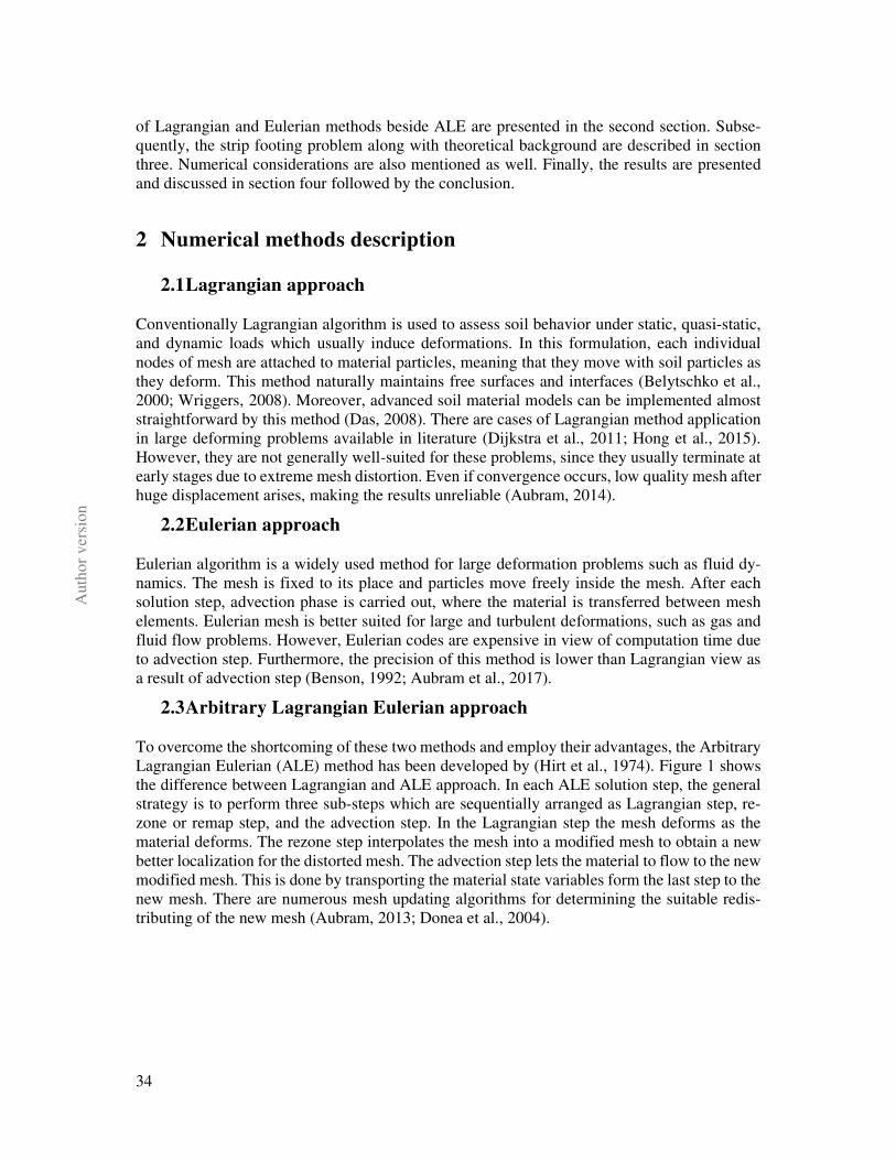
To overcome the shortcoming of these two methods and employ their advantages, the Arbitrary Lagrangian Eulerian (ALE) method has been developed by (Hirt et al., 1974). Figure 1 shows the difference between Lagrangian and ALE approach. In each ALE solution step, the general strategy is to perform three sub-steps which are sequentially arranged as Lagrangian step, re-zone or remap step, and the advection step. In the Lagrangian step the mesh deforms as the material deforms. The rezone step interpolates the mesh into a modified mesh to obtain a new better localization for the distorted mesh. The advection step lets the material to flow to the new modified mesh. This is done by transporting the material state variables form the last step to the new mesh. There are numerous mesh updating algorithms for determining the suitable redis-tributing of the new mesh (Aubram, 2013; Donea et al., 2004).

35

Aut

hor

vers

ion

Figure 1: FE model Initial configuration (left), Material deformation in a Lagrangian analysis

(middle) and an Arbitrary Lagrangian Eulerian analysis ALE (right)

3 Numerical Model Description

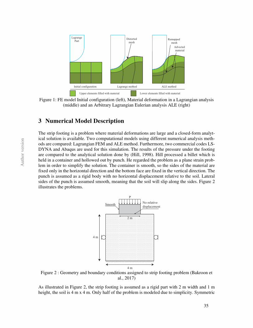
The strip footing is a problem where material deformations are large and a closed-form analyt-ical solution is available. Two computational models using different numerical analysis meth-ods are compared: Lagrangian FEM and ALE method. Furthermore, two commercial codes LS-DYNA and Abaqus are used for this simulation. The results of the pressure under the footing are compared to the analytical solution done by (Hill, 1998). Hill processed a billet which is held in a container and hollowed out by punch. He regarded the problem as a plane strain prob-lem in order to simplify the solution. The container is smooth, so the sides of the material are fixed only in the horizontal direction and the bottom face are fixed in the vertical direction. The punch is assumed as a rigid body with no horizontal displacement relative to the soil. Lateral sides of the punch is assumed smooth, meaning that the soil will slip along the sides. Figure 2 illustrates the problems.

Figure 2 : Geometry and boundary conditions assigned to strip footing problem (Bakroon et

al., 2017)

As illustrated in Figure 2, the strip footing is assumed as a rigid part with 2 m width and 1 m height, the soil is 4 m x 4 m. Only half of the problem is modeled due to simplicity. Symmetric

Upper elements filled with material Lower elements filled with material

Remapped

mesh

Advected

material

Distorted

mesh

Initial configuration ALE methodLagrange method

Lagrange

Part

4 m

4 m

Smooth

2 m

No relative

displacement

P

36

Aut

hor

vers

ion

boundary conditions are imposed on the plane of symmetry by prescribing fixed condition in the normal direction. The plane strain condition is applied. For the ratio of base over soil width = 0.5, the maximum punch pressure for this problem can

be calculated with ���� = 2�(1 +�

� ) where � is the soil shear strength (Hill, 1950).

The soil material parameters used in the problem are shown in Table 1, where � is Poisson ratio and � is the modulus of elasticity. The Tresca constitutive model is adopted.

Table 1 : Material parameters for the soft soil

� [kPa] � [kPa] � [-]

2980 10 0.49

In Abaqus, a 4-node bilinear plane strain quadrilateral with reduced integration and hourglass control (Abaqus element type CPE4R) is used. The rigid body elements were meshed by a 2-node 2D linear rigid link (R2D2). In LS-DYNA, 1-point ALE element were used (ELFORM 5 in *SECTION_SOLID keyword). The rigid body was modelled with the reduced 4-point element formulation (ELFORM 1). This is an efficient formulation which is applicable to general cases. For both softwares the rigid footing nodes were tied to soil’s surface nodes to reduce model dependency on contact. Frictionless tangential penalty contact between the lateral side of the footing and the top soil surface is defined to allow sliding between soil and foundation. Among various smoothing methods, equipotential algorithm as described in (Winslow, 1963) was used for both LS-DYNA and Abaqus. This smoothing algorithm is more commonly used and provides more stable results (Dassault Systèmes, 2016). In this smoothing method, by solv-ing Laplace equations the new mesh is drawn. For advection step, there are two methods avail-able in LS-DYNA: Donor cell and Van Leer. Van Leer method is preferred over donor cell since it benefits from second order accuracy and is more stable (Hallquist, 2016). Therefore, Van Leer advection method was used.

4 Results

In this section, the comparison between Lagrangian and ALE method is presented. The same problem was used by (Qiu et al., 2011) to compare the results of implicit, explicit Lagrangian, and CEL formulation. The results of this study were comparable with values calculated by (Qiu et al., 2011). Afterwards, a thorough investigation for a 2D Lagrangian and ALE performance comparison was made such as mesh size optimization, ALE remapping step, analysis time com-parison, and effect of time step size. The simulations are carried out using a server at TU Berlin with two 2.93 GHz quad-core Intel CPU X5570 and 48 GB of RAM. Due to limited number of elements in the model, only one core of the CPU was used to scale up the computation time. The utilized versions of codes were LS-DYNA R9.1.0 and Abaqus 2017. The comparison is conducted based on pressure results and computation time. In the following sub-sections, different criteria and considerations were studied and discussed.

37

Aut

hor

vers

ion

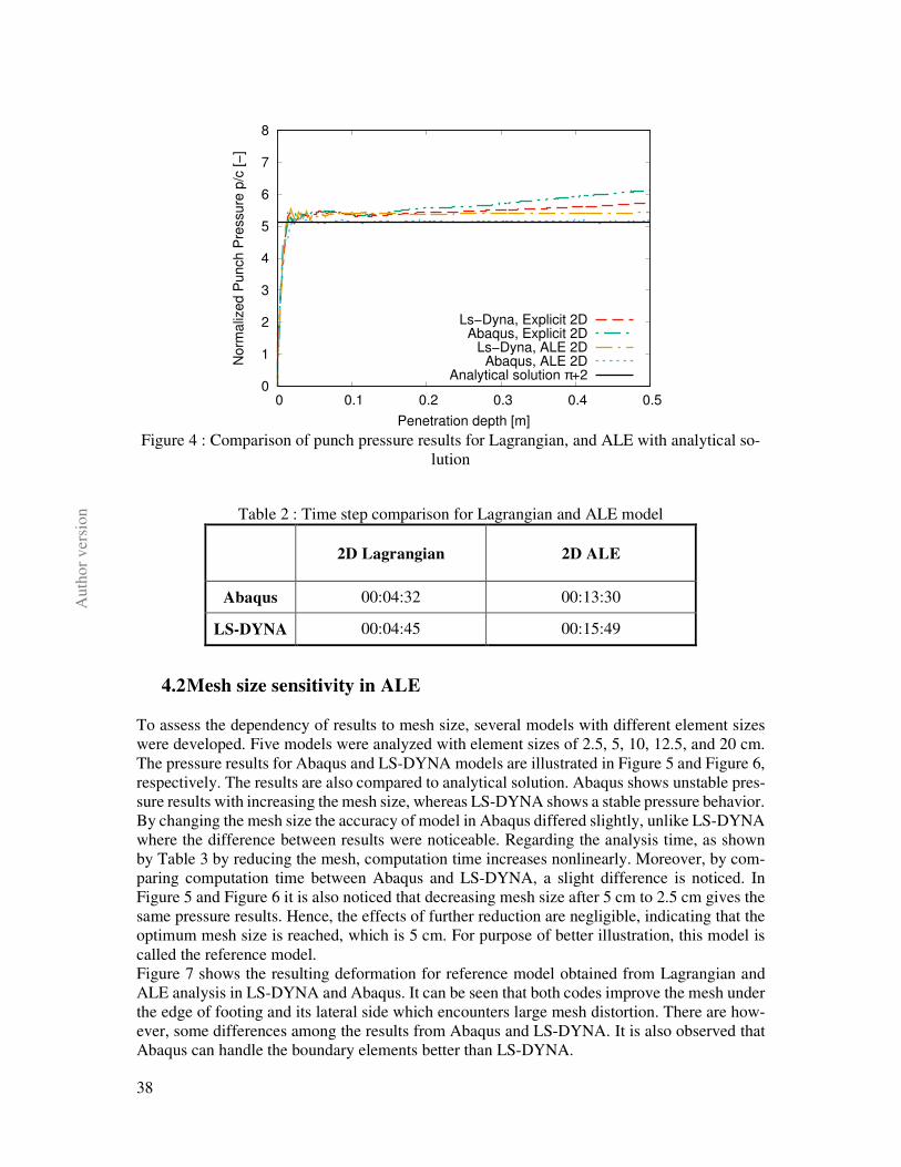
4.1 Model Verification

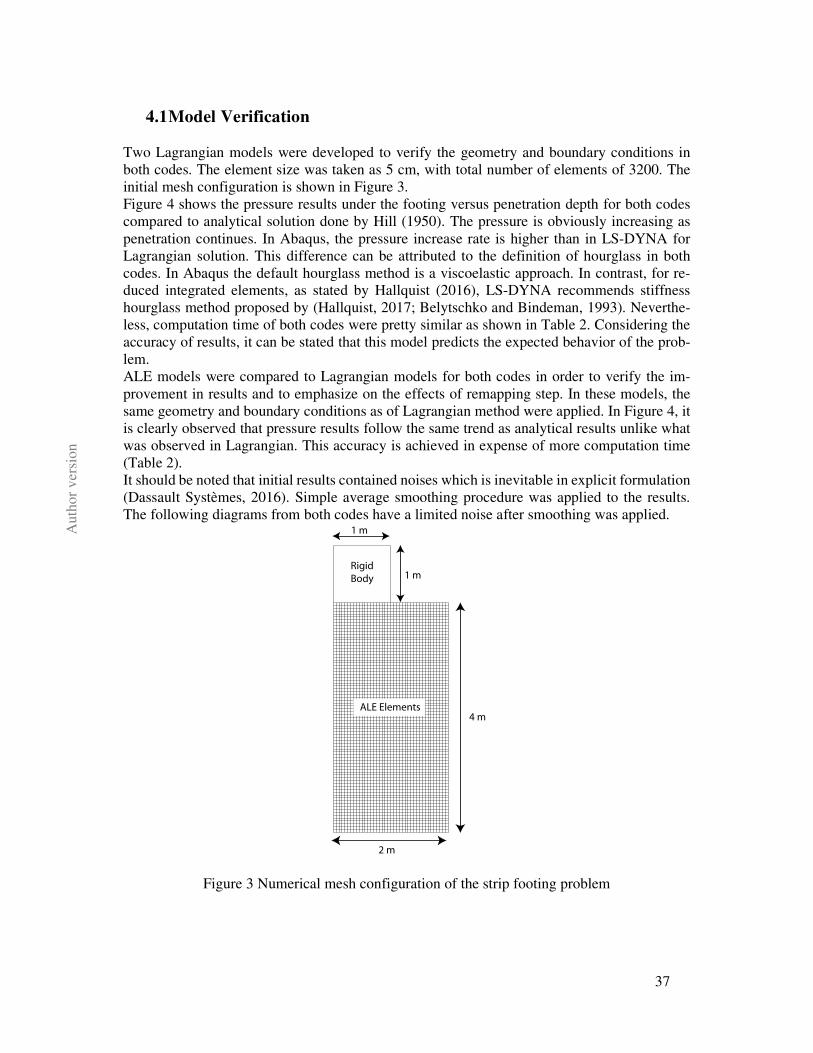
Two Lagrangian models were developed to verify the geometry and boundary conditions in both codes. The element size was taken as 5 cm, with total number of elements of 3200. The initial mesh configuration is shown in Figure 3. Figure 4 shows the pressure results under the footing versus penetration depth for both codes compared to analytical solution done by Hill (1950). The pressure is obviously increasing as penetration continues. In Abaqus, the pressure increase rate is higher than in LS-DYNA for Lagrangian solution. This difference can be attributed to the definition of hourglass in both codes. In Abaqus the default hourglass method is a viscoelastic approach. In contrast, for re-duced integrated elements, as stated by Hallquist (2016), LS-DYNA recommends stiffness hourglass method proposed by (Hallquist, 2017; Belytschko and Bindeman, 1993). Neverthe-less, computation time of both codes were pretty similar as shown in Table 2. Considering the accuracy of results, it can be stated that this model predicts the expected behavior of the prob-lem. ALE models were compared to Lagrangian models for both codes in order to verify the im-provement in results and to emphasize on the effects of remapping step. In these models, the same geometry and boundary conditions as of Lagrangian method were applied. In Figure 4, it is clearly observed that pressure results follow the same trend as analytical results unlike what was observed in Lagrangian. This accuracy is achieved in expense of more computation time (Table 2). It should be noted that initial results contained noises which is inevitable in explicit formulation (Dassault Systèmes, 2016). Simple average smoothing procedure was applied to the results. The following diagrams from both codes have a limited noise after smoothing was applied.

Figure 3 Numerical mesh configuration of the strip footing problem

1 m

1 mRigid

Body

4 m

2 m

ALE Elements

38

Aut

hor

vers

ion

Figure 4 : Comparison of punch pressure results for Lagrangian, and ALE with analytical so-

lution

Table 2 : Time step comparison for Lagrangian and ALE model

2D Lagrangian 2D ALE

Abaqus 00:04:32 00:13:30

LS-DYNA 00:04:45 00:15:49

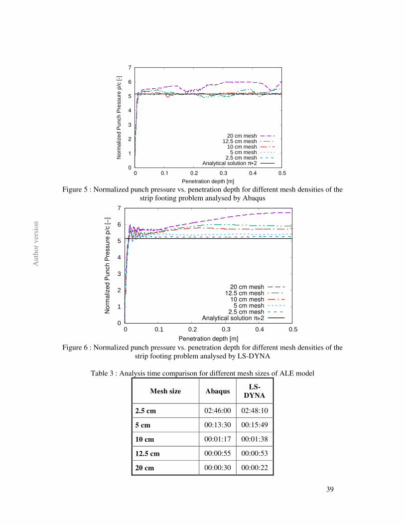
4.2 Mesh size sensitivity in ALE

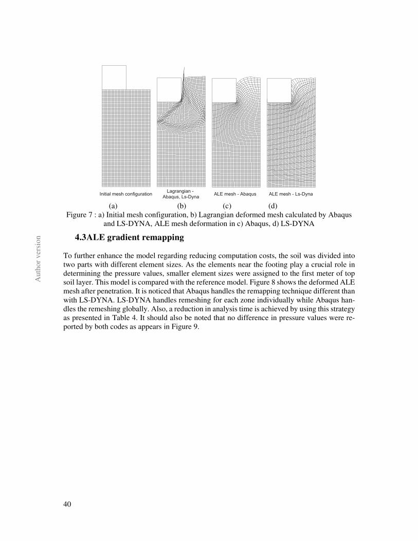
To assess the dependency of results to mesh size, several models with different element sizes were developed. Five models were analyzed with element sizes of 2.5, 5, 10, 12.5, and 20 cm. The pressure results for Abaqus and LS-DYNA models are illustrated in Figure 5 and Figure 6, respectively. The results are also compared to analytical solution. Abaqus shows unstable pres-sure results with increasing the mesh size, whereas LS-DYNA shows a stable pressure behavior. By changing the mesh size the accuracy of model in Abaqus differed slightly, unlike LS-DYNA where the difference between results were noticeable. Regarding the analysis time, as shown by Table 3 by reducing the mesh, computation time increases nonlinearly. Moreover, by com-paring computation time between Abaqus and LS-DYNA, a slight difference is noticed. In Figure 5 and Figure 6 it is also noticed that decreasing mesh size after 5 cm to 2.5 cm gives the same pressure results. Hence, the effects of further reduction are negligible, indicating that the optimum mesh size is reached, which is 5 cm. For purpose of better illustration, this model is called the reference model. Figure 7 shows the resulting deformation for reference model obtained from Lagrangian and ALE analysis in LS-DYNA and Abaqus. It can be seen that both codes improve the mesh under the edge of footing and its lateral side which encounters large mesh distortion. There are how-ever, some differences among the results from Abaqus and LS-DYNA. It is also observed that Abaqus can handle the boundary elements better than LS-DYNA.

0

1

2

3

4

5

6

7

8

0 0.1 0.2 0.3 0.4 0.5

No

rma

lize

d P

un

ch

Pre

ssu

re p

/c [

−]

Penetration depth [m]

Ls−Dyna, Explicit 2DAbaqus, Explicit 2D

Ls−Dyna, ALE 2DAbaqus, ALE 2D

Analytical solution π+2

39

Aut

hor

vers

ion

Figure 5 : Normalized punch pressure vs. penetration depth for different mesh densities of the

strip footing problem analysed by Abaqus

Figure 6 : Normalized punch pressure vs. penetration depth for different mesh densities of the

strip footing problem analysed by LS-DYNA

Table 3 : Analysis time comparison for different mesh sizes of ALE model

Mesh size Abaqus LS-

DYNA

2.5 cm 02:46:00 02:48:10

5 cm 00:13:30 00:15:49

10 cm 00:01:17 00:01:38

12.5 cm 00:00:55 00:00:53

20 cm 00:00:30 00:00:22

0

1

2

3

4

5

6

7

0 0.1 0.2 0.3 0.4 0.5

Nor

mal

ized

Pun

ch P

ress

ure

p/c

[-]

Penetration depth [m]

20 cm mesh12.5 cm mesh

10 cm mesh5 cm mesh

2.5 cm meshAnalytical solution π+2

0

1

2

3

4

5

6

7

0 0.1 0.2 0.3 0.4 0.5

Norm

aliz

ed P

unch P

ressure

p/c

[−

]

Penetration depth [m]

20 cm mesh12.5 cm mesh

10 cm mesh5 cm mesh

2.5 cm meshAnalytical solution π+2

40

Aut

hor

vers

ion

(a) (b) (c) (d)

Figure 7 : a) Initial mesh configuration, b) Lagrangian deformed mesh calculated by Abaqus and LS-DYNA, ALE mesh deformation in c) Abaqus, d) LS-DYNA

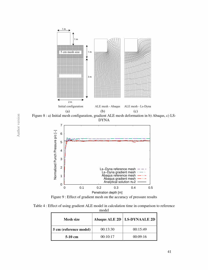
4.3 ALE gradient remapping

To further enhance the model regarding reducing computation costs, the soil was divided into two parts with different element sizes. As the elements near the footing play a crucial role in determining the pressure values, smaller element sizes were assigned to the first meter of top soil layer. This model is compared with the reference model. Figure 8 shows the deformed ALE mesh after penetration. It is noticed that Abaqus handles the remapping technique different than with LS-DYNA. LS-DYNA handles remeshing for each zone individually while Abaqus han-dles the remeshing globally. Also, a reduction in analysis time is achieved by using this strategy as presented in Table 4. It should also be noted that no difference in pressure values were re-ported by both codes as appears in Figure 9.

ALE mesh - Ls-DynaALE mesh - AbaqusInitial mesh configurationLagrangian -

Abaqus, Ls-Dyna

41

Aut

hor

vers

ion

(a) (b) (c)

Figure 8 : a) Initial mesh configuration, gradient ALE mesh deformation in b) Abaqus, c) LS-DYNA

Figure 9 : Effect of gradient mesh on the accuracy of pressure results

Table 4 : Effect of using gradient ALE model in calculation time in comparison to reference

model

Mesh size Abaqus ALE 2D LS-DYNAALE 2D

5 cm (reference model) 00:13:30 00:15:49

5-10 cm 00:10:17 00:09:16

Initial configuration ALE mesh - Abaqus ALE mesh - Ls-Dyna

1 m

1 m

1 m

3 m

2 m

10 cm mesh size

5 cm mesh size

0

1

2

3

4

5

6

7

0 0.1 0.2 0.3 0.4 0.5

No

rma

lize

d P

un

ch

Pre

ssu

re p

/c [

−]

Penetration depth [m]

Ls−Dyna reference meshLs−Dyna gradient meshAbaqus reference mesh

Abaqus gradient meshAnalytical solution π+2

42

Aut

hor

vers

ion

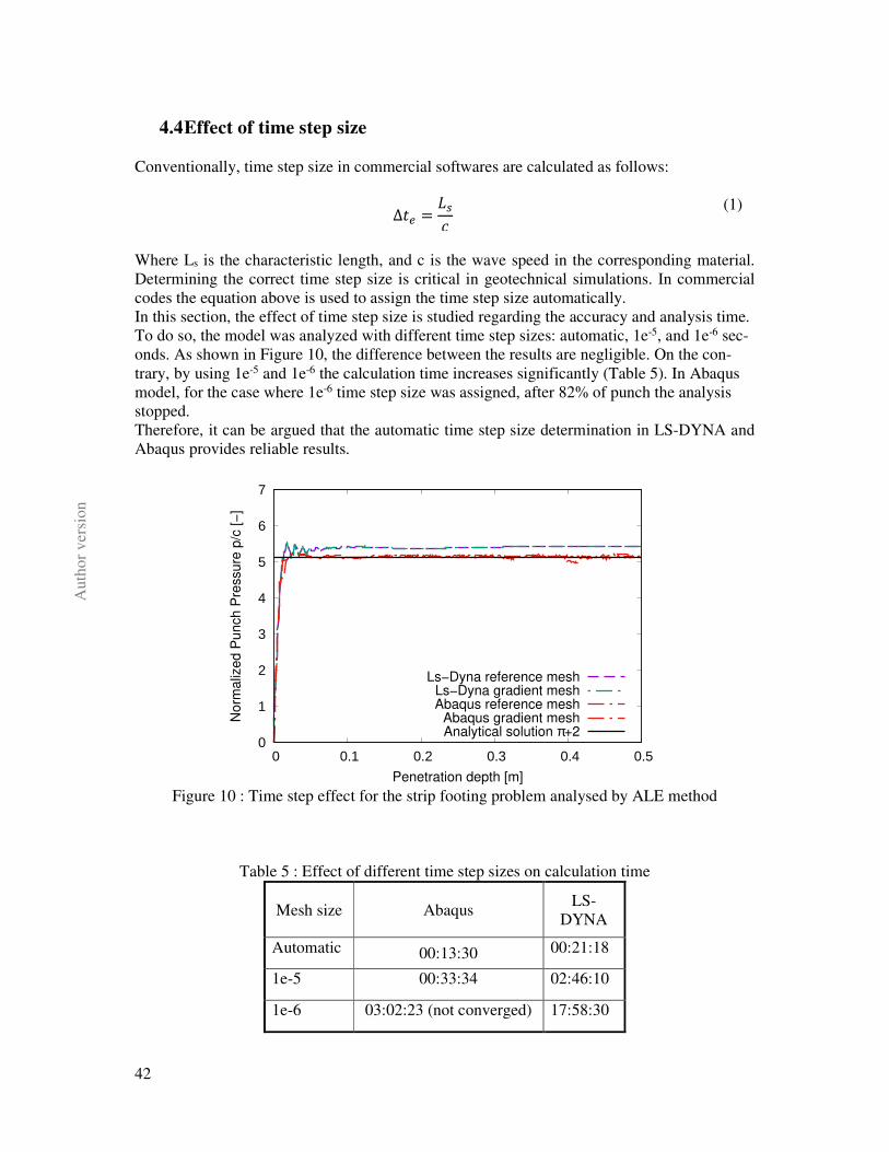
4.4 Effect of time step size

Conventionally, time step size in commercial softwares are calculated as follows:

∆�� =��

�

(1)

Where Ls is the characteristic length, and c is the wave speed in the corresponding material. Determining the correct time step size is critical in geotechnical simulations. In commercial codes the equation above is used to assign the time step size automatically. In this section, the effect of time step size is studied regarding the accuracy and analysis time. To do so, the model was analyzed with different time step sizes: automatic, 1e-5, and 1e-6 sec-onds. As shown in Figure 10, the difference between the results are negligible. On the con-trary, by using 1e-5 and 1e-6 the calculation time increases significantly (Table 5). In Abaqus model, for the case where 1e-6 time step size was assigned, after 82% of punch the analysis stopped. Therefore, it can be argued that the automatic time step size determination in LS-DYNA and Abaqus provides reliable results.

Figure 10 : Time step effect for the strip footing problem analysed by ALE method

Table 5 : Effect of different time step sizes on calculation time

Mesh size Abaqus LS-

DYNA

Automatic 00:13:30 00:21:18

1e-5 00:33:34 02:46:10

1e-6 03:02:23 (not converged) 17:58:30

0

1

2

3

4

5

6

7

0 0.1 0.2 0.3 0.4 0.5

No

rma

lize

d P

un

ch

Pre

ssu

re p

/c [

−]

Penetration depth [m]

Ls−Dyna reference meshLs−Dyna gradient meshAbaqus reference mesh

Abaqus gradient meshAnalytical solution π+2

43

Aut

hor

vers

ion

Conclusion

In this research a strip footing problem, for which an analytical solution is available, has been simulated by two commercial codes Abaqus and LS-DYNA. ALE method capabilities in ge-otechnical applications were evaluated by comparing the results to Lagrangian method. Alt-hough the Lagrangian solution converged, the mesh quality reduced drastically after app. 25 cm of penetration. In contrast, by using remapping feature in ALE, the level of mesh distortion was limited, and therefore the accuracy and reliability of the results was increased. In order to study the mesh size effect, five mesh sizes where used: 2.5, 5, 10, 12.5, and 20 cm. The Abaqus results showed an accurate behaviour in comparison to the analytical solution with noticeable fluctuations. On the other hand, the LS-DYNA results shows stable solutions but in expense of losing accuracy. Automatic time step size allocations feature in both codes were compared to smaller manual max. time step assignment. It was observed that there is no significant improvement in results by decreasing time step sizes. This shows the robustness of automatic time step size technique implemented in both Abaqus and LS-DYNA. Computation time was also evaluated between Abaqus and LS-DYNA. In case of using large mesh sizes, no major difference was observed. However, by using finer meshes the computation cost of Abaqus was less compared to LS-DYNA. Comparing pressure values with empirical solution, the error of Abaqus was less than 1% while the error of LS-DYNA was less than 5%.

References

[1] Aubram D., Rackwitz F., Wriggers P., and Savidis S. A. (2015): An ALE method for penetration into sand utilizing optimization-based mesh motion. Computers and Geotech-

nics, 65:241-249.

[2] Dijkstra J., Broere W., and Heeres O. M. (2011): Numerical simulation of pile installa-tion. Computers and Geotechnics, 38 (5):612-622.

[3] Konkol J., and Bałachowski L. (2016): Large deformation finite element analysis of un-drained pile installation. Studia Geotechnica et Mechanica, 38 (1).

[4] Belytschko, Ted; Liu, W. K.; Moran, B. (2000): Nonlinear finite elements for continua and structures. Chichester: John Wiley.

[5] Wriggers, P. (2008): Nonlinear finite element methods. Berlin, London: Springer.

[6] Das, Braja M. (2008): Advanced soil mechanics. 3rd ed. London: Taylor & Francis.

[7] Hong Y., Soomro M. A., Ng C., Wang L. Z., Yan J. J., and Li B. (2015): Tunnelling under pile groups and rafts. Numerical parametric study on tension effects. Computers and

Geotechnics, 68:54-65.

[8] Aubram D. (2014): Über die Berücksichtigung großer Bodendeformationen in numerischen Modellen. Vorträge zum Ohde-Kolloquium, Dresden, Germany:109-122.

[9] Benson D. (1992): Computational methods in Lagrangian and Eulerian hydrocodes. Com-

puter Methods in Applied Mechanics and Engineering, 99:235-394.

44

Aut

hor

vers

ion

[10] Aubram D., Rackwitz F., and Savidis S. A. (2017): Contribution to the Non-Lagrangian Formulation of Geotechnical and Geomechanical Processes. In: Theodoros Triantafyl-lidis (Hg.): Holistic Simulation of Geotechnical Installation Processes: Theoretical Re-sults and Applications: Springer International Publishing:53-100.

[11] Hirt C. W., Amsden A. A., and Cook J. L. (1974): An Arbitrary Lagrangian-Eulerican Computing Method for All Flow Speeds. JOURNAL OF COMPUTATIONAL PHYSICS,

14:227-253.

[12] Aubram, D. (2013): Arbitrary Lagrangian-Eulerian method for penetration into sand at finite deformations. Germany: Shaker Verlag, Aachen.

[13] Donea, J.; Huerta, A.; Ponthot, J.-Ph.; Rodriguez-Ferran, A. (2004): Arbitrary Lagran-gian–Eulerian Methods: John Wiley & Sons, Ltd (1).

[14] Hill, R. (1998): The mathematical theory of plasticity. Oxford: Clarendon Press (Oxford classic texts in the physical sciences, 11).

[15] Bakroon, M.; Aubram, D.; Rackwitz, F. (Hg.) (2017): Geotechnical large deformation numerical analysis using implicit and explicit integration (In review). 3rd International Conference on New Advances in Civil Engineering.

[16] Winslow A. M. (1963): Equipotential Zoning of Two-Dimensional Meshes. Lawrence

Radiation Laboratory, University of California.

[17] Dassault Systèmes (2016): Abaqus. Version 2016 documentation. Version 2016.

[18] Hallquist, J. O. (2016): Ls-Dyna Theory Manual.

[19] Qiu G., Henke S., and Grabe J. (2011): Application of a Coupled Eulerian–Lagrangian approach on geomechanical problems involving large deformations. Computers and Ge-

otechnics, 38 (1):30-39.

[20] Hallquist J. O. (2017): LS-DYNA. Theoretical manual. Version. Livermore: Livermore Software Technology Corporation.

[21] Belytschko T., and Bindeman L. P. (1993): Assumed strain stabilization of the eight node hexahedral element. Computer Methods in Applied Mechanics and Engineering, 105 (2):225-260.

Authors

Montaser Bakroon M.Sc., Reza Daryaei M.Sc., Dr.-Ing. Daniel Aubram, Prof. Dr.-Ing. Frank Rackwitz Technische Universität Berlin Fachgebiet Grundbau und Bodenmechanik Gustav-Meyer-Allee 25 13355 Berlin Tel.: +49 (0) 30 - 314 72341 Fax: +49 (0) 40 - 314 72343 e-mail: info@grundbau.tu-berlin.de Web: www.grundbau.tu-berlin.de