applications of coupled eulerian-lagrangian method to ... · pdf fileapplications of coupled...

2009 SIMULIA Customer Conference 1

Applications of Coupled Eulerian-Lagrangian Method to Geotechnical Problems with Large

Deformations

G. Qiu, S. Henke, and J. Grabe

Institute of Geotechnical and Construction Engineering, Hamburg University of Technology, Germany

Abstract: In recent years, finite element method has been considered the main tool for solving geomechanical boundary value problems. Studying geotechnical problems like collapse analysis of a quay wall construction or pile penetration into the subsoil, it is evident that large deformation of the soil body can occur. The main problems in these analyses are contact problems and large deformations of the FE-mesh. Abaqus, version 6.8 now provides a new tool, the Coupled Eulerian-Lagrangian method (CEL), to deal with large deformation problems. With this new method the drawback of the FE-method, which originates from its reliance on a lagrangian mesh, can be overcome. In this paper, two benchmark problems are analyzed using the CEL-method, the results are compared to classic implicit- and explicit-solutions. Concluding, the application of CEL for pile penetration analysis is investigated.

Keywords: Abaqus, finite element method, Coupled Eulerian-Lagrangian, large deformation analysis, soil mechanics, geotechnics, strip footing, anchor plate, pile penetration.

1. Introduction

In recent years, finite element method has been considered the main tool for solving geotechnical problems. A three-dimensional FE-simulation of a quay wall construction in service state at the port of Hamburg has been done by Mardfeldt (2005). Regarding exceptional load cases like extreme tide, scouring, or grounding of a ship the quay wall construction may reach its limit state. In such cases large deformations of the soil and the structure can occur. Another application with large deformations in geotechnical engineering is the analysis of pile penetration into the subsoil. Several researchers investigated the pile penetration process using finite element method. First investigations have been made by Mabsout and Tassoulas (1994) using a special zipper-type-technique to allow the simulation of discrete hammer blows on a prebored pile. This technique has been extended by Cudmani (2001) to simulate the cone penetration test using an axisymmetric model. A comparison of different pile installation methods (pile jacking, vibratory pile driving, impact pile driving) has been done by Mahutka et al. (2006). These investigations are also constrained to axisymmetric calculations. Henke and Grabe (2006) extended this modeling

2 2009 SIMULIA Customer Conference

technique to allow three-dimensional analyses of pile installation so that the installation of piles with open cross-section is possible (Henke and Hügel, 2007).

It is evident that finite element method has many problems solving geotechnical problems with large deformations. Especially, contact problems and large mesh distortions may occur so that a convergent solution often cannot be found. In this paper, simulations of large deformation problems using Abaqus’ newly built-in feature CEL are fulfilled and the results are compared to those received by classical implicit and explicit calculations to show the capabilities of this tool.

2. Numerical methods

2.1 Implicit analysis

The implicit solver is implemented in Abaqus/Standard. Because of implemented convergence criteria the implicit solver is implicitly stable. The implicit procedure uses an automatic incremental strategy based on the success rate of a full Newton iterative solution method. For every step the quantities of the time step t and t+t are taken into account. This means that for every time step a nonlinear system of equations has to be solved using e.g. Newmarks method.

2.2 Explicit analysis

The explicit solver is a numerical solution algorithm to solve the equation of motion:

fKuuCuM

Using the explicit solver the equation of motion is solved for a certain time step by direct integration using the central difference rule. This method is especially effective, if a lumped or diagonal mass matrix exists. In this case, the unknown deformations appear only at one side of the system of equations so that the solution is easy to receive. The explicit solution procedure is not implicitly stable. A stable time increment tcrit has to be defined for which the solution is conditionally stable.

d

ecrit c

Lt

Le is the minimum element length and cd the dilatory wave speed. The main problem using an explicit solver is that solution control is very difficult because no convergence criterion exists.

2.3 Coupled Eulerian-Lagrangian (CEL) analysis

If a continuum deforms or flows, the position of the small volumetric elements changes with time. These positions can be described as functions of time in two ways:

Lagrangian description: the movement of the continuum is specified as a function of its initial coordinates and time.


Eulerian description: the movement of the continuum is specified as a function of its instantaneous position and time.

In simulations with Lagrangian formulation the interface between two parts is precisely defined and tracked. In these simulations large deformation of a part leads to hopeless mesh and element distortion. In Eulerian analysis a Eulerian reference mesh, which remains undistorted and does not move, is needed, to trace the motion of the particles. The advantage of a Eulerian formulation is that no element distortions occur. Disadvantageously, the interface between two parts cannot be described as precise as if a Lagrangian formulation is used. Numerical diffusion can happen during the simulation. A Coupled Eulerian-Lagrangian (CEL) method, which attempts to capture the strength of the Lagrangian and the Eulerian method, is implemented in Abaqus/Explicit. For general geotechnical problems, a Lagrangian mesh is used to discretize structures, while a Eulerian mesh is used to discretize the subsoil. The interface between structure and subsoil can be represented using the boundary of the Lagrangian domain. On the other hand, the Eulerian mesh, which represents the soil that may experience large deformations, has no problems regarding mesh and element distortions.

3. Benchmark

3.1 Strip footing problem

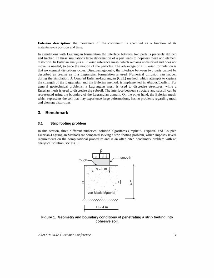
In this section, three different numerical solution algorithms (Implicit-, Explicit- and Coupled Eulerian-Lagrangian Method) are compared solving a strip footing problem, which imposes severe requirements on the computational procedure and is an often cited benchmark problem with an analytical solution, see Fig. 1.

D = 4 m

4 m

d = 2 m

p

smoothrough

von Mises Material

Figure 1. Geometry and boundary conditions of penetrating a strip footing into cohesive soil.


This plane strain problem has been analytically solved by Hill (1950) using the slip line theory. According to Hill (1950) the maximum punch pressure for this problem with a ratio d/D = 0.5 (Fig. 1) can be calculated with:

cp )2( ,

where c is the shear strength of the soil which is described using a von MISES material.

Numerical analyses have been executed by van Langen (1991) using a TRESCA material. Analogue to his work in this study the von MISES material parameters in Tab. 1 are used for the analyses.

Table 1. Material parameters for cohesive soil.

Property G c [kpa] [-] [kPa] Value 1000 0.49 10

The side of the footing is modeled smooth, whereas the base is rough. The footing, which penetrates into a cohesive but weightless soil with dimension 4 m x 4 m, has a width of 2 m and a height of 1 m. The strip footing is discretized as a rigid body. The plane strain problem is modeled two-dimensionally using the implicit- and the explicit-solution algorithm. The subsoil is meshed using linear elements with reduced integration (element type: CPE4R). Regarding the Coupled Eulerian-Lagrangian analysis the penetration process must be simulated three-dimensionally. Three-dimensional Eulerian elements are used to discretize the soil body (element type: EC3D8R).

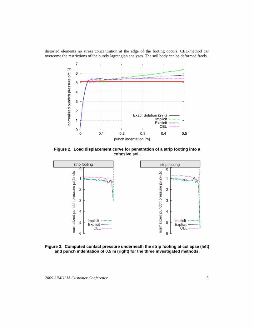
The load-displacement curves that have been obtained out of the comparative analyses are depicted in Fig. 2. The maximum reaction force is reached at a punch indentation of less than 0.1 m in all analyses. The agreement between numerical solutions and the analytical solution is very satisfactory. The difference remains within 8%. After reaching a maximum reaction force the solution of the CEL-analysis remains nearly constant, whereas the solution of implicit- and explicit-method increases continuously.

The increasing reaction force in the implicit analysis can be explained considering Fig. 3. This figure shows the calculated contact stresses underneath the strip footing for the three investigated methods. Stress concentrations can be seen at the edge of the footing regarding the implicit calculation which cannot be explained physically. According to the theoretical solution, the contact pressure cannot be greater than c)2( . The contact pressure must be evenly distributed

at the bottom of the footing. There should be no stress concentration at the corner of the footing. In contrast, the stress concentration at the corner regarding the implicit analysis increases with growing punch indentation. As shown in Fig. 4, the velocity gradient near the edge of the footing is very high. The soil is pushed down, slips sideways and then moves upwards. The velocity field is not uniquely to define. This point is well known as singular plasticity point. The velocity gradient is too high to be simulated using the implicit method. The soil nearby the corner can only move down and than moves sideways. An upward motion cannot be found in Fig. 4. To overcome the effect of singular plasticity points, van Langen (1991) incorporated some potential slip lines into his implicit model. Regarding the explicit analysis the element at the edge of the footing is distorted extremely. Furthermore, an upward motion cannot be found, too. Due to the observed


distorted elements no stress concentration at the edge of the footing occurs. CEL-method can overcome the restrictions of the purely lagrangian analyses. The soil body can be deformed freely.

0

1

2

3

4

5

6

7

0 0.1 0.2 0.3 0.4 0.5

norm

aliz

ed p

undc

h pr

essu

re p

/c [-

]

punch indentation [m]

Exact Solution (2+π)ImplicitExplicit

CEL

Figure 2. Load displacement curve for penetration of a strip footing into a cohesive soil.

norm

aliz

ed p

undc

h pr

essu

re p

/(2+

)c

strip footing

ImplicitExplicit

CEL 6

5

4

3

2

1

0

norm

aliz

ed p

undc

h pr

essu

re p

/(2+

)c

ImplicitExplicit

CEL 6

5

4

3

2

1

0

strip footing

Figure 3. Computed contact pressure underneath the strip footing at collapse (left) and punch indentation of 0.5 m (right) for the three investigated methods.


Implicit Explicit CEL

Figure 4. Velocity field of the strip footing problem after a punch indentation of 0.5 m for the three investigated numerical methods .

3.2 Anchor plate problem

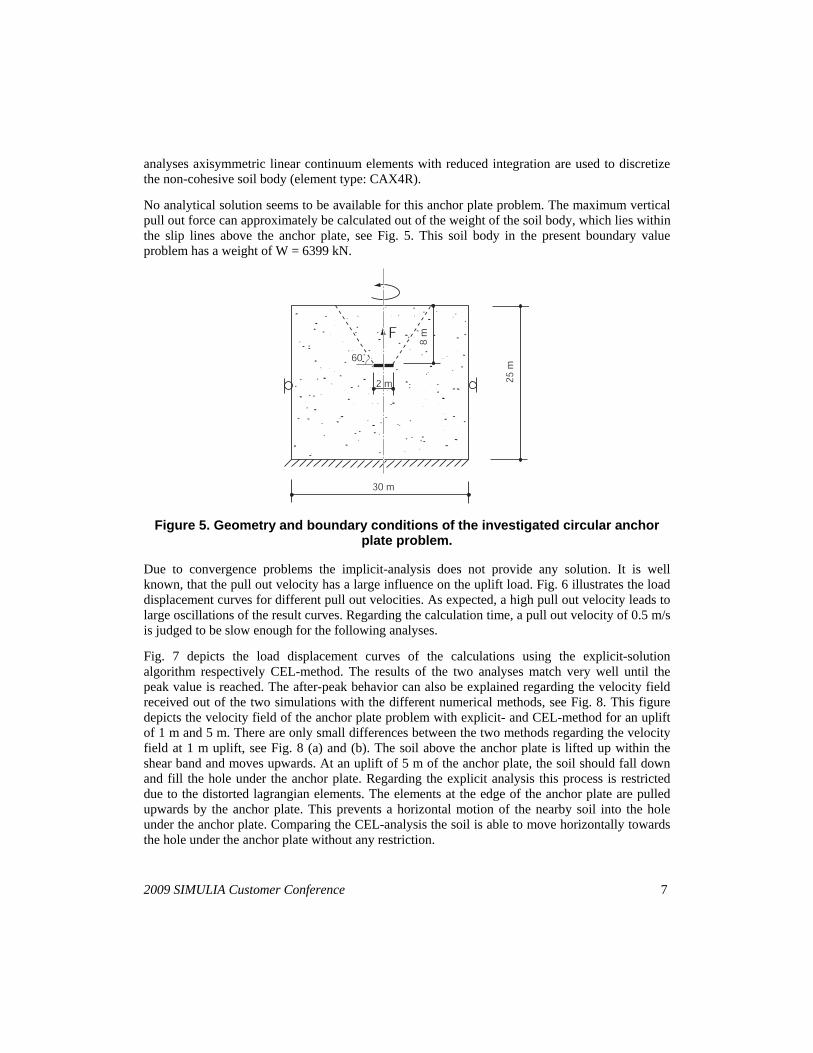
In this section, the three investigated numerical methods are used to solve a circular anchor plate problem. A smooth circular anchor plate, with a radius of 1 m and a thickness of 0.1 m, is pulled out of a non-cohesive soil, see Fig. 5. The soil has a friction angle = 30°. The Druck-Prager material model is used to simulate the soil. In this material model the friction angle is needed which can be calculated as follows:

sin3

sin6tan

.

The used material parameters are given in table 2.

Table 2. Material parameters for non-cohesive soil.

Property E K ρ [kPa] [-] [°] [-] [t] Value 35000 0.3 50.2 1.0 2.0

The pull out process is simulated axially symmetric in the implicit- and explicit-analysis, whereas the CEL-analysis has to be done three-dimensionally. Same as in the strip footing problem the anchor plate is modeled as a rigid body. Three-dimensional Eulerian elements are used to discretize the soil (element type: EC3D8R) in the CEL analysis. In the implicit- and explicit


analyses axisymmetric linear continuum elements with reduced integration are used to discretize the non-cohesive soil body (element type: CAX4R).

No analytical solution seems to be available for this anchor plate problem. The maximum vertical pull out force can approximately be calculated out of the weight of the soil body, which lies within the slip lines above the anchor plate, see Fig. 5. This soil body in the present boundary value problem has a weight of W = 6399 kN.

F

30 m

25 m

2 m

8 m

60˚

Figure 5. Geometry and boundary conditions of the investigated circular anchor plate problem.

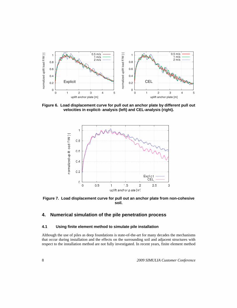
Due to convergence problems the implicit-analysis does not provide any solution. It is well known, that the pull out velocity has a large influence on the uplift load. Fig. 6 illustrates the load displacement curves for different pull out velocities. As expected, a high pull out velocity leads to large oscillations of the result curves. Regarding the calculation time, a pull out velocity of 0.5 m/s is judged to be slow enough for the following analyses.

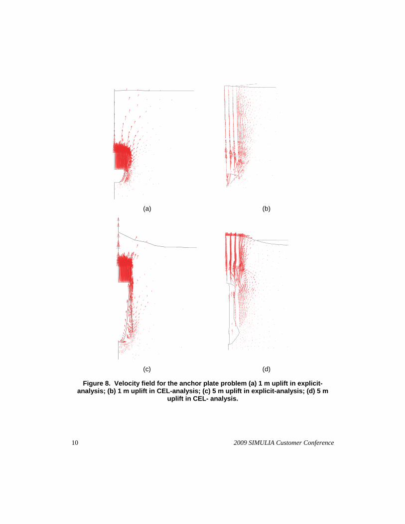
Fig. 7 depicts the load displacement curves of the calculations using the explicit-solution algorithm respectively CEL-method. The results of the two analyses match very well until the peak value is reached. The after-peak behavior can also be explained regarding the velocity field received out of the two simulations with the different numerical methods, see Fig. 8. This figure depicts the velocity field of the anchor plate problem with explicit- and CEL-method for an uplift of 1 m and 5 m. There are only small differences between the two methods regarding the velocity field at 1 m uplift, see Fig. 8 (a) and (b). The soil above the anchor plate is lifted up within the shear band and moves upwards. At an uplift of 5 m of the anchor plate, the soil should fall down and fill the hole under the anchor plate. Regarding the explicit analysis this process is restricted due to the distorted lagrangian elements. The elements at the edge of the anchor plate are pulled upwards by the anchor plate. This prevents a horizontal motion of the nearby soil into the hole under the anchor plate. Comparing the CEL-analysis the soil is able to move horizontally towards the hole under the anchor plate without any restriction.


0

0.2

0.4

0.6

0.8

1

0 1 2 3 4 5

norm

aliz

ed u

plift

load

F/W

[-]

uplift anchor plate [m]

0.5 m/s1 m/s2 m/s

Explicit

0

0.2

0.4

0.6

0.8

1

0 1 2 3 4 5

norm

aliz

ed u

plift

load

F/W

[-]

uplift anchor plate [m]

0.5 m/s1 m/s2 m/s

CEL

Figure 6. Load displacement curve for pull out an anchor plate by different pull out velocities in explicit- analysis (left) and CEL-analysis (right).

Figure 7. Load displacement curve for pull out an anchor plate from non-cohesive soil.

4. Numerical simulation of the pile penetration process

4.1 Using finite element method to simulate pile installation

Although the use of piles as deep foundations is state-of-the-art for many decades the mechanisms that occur during installation and the effects on the surrounding soil and adjacent structures with respect to the installation method are not fully investigated. In recent years, finite element method


is used by many authors to simulate a part or even the whole penetration process. Mainly, there are three different approaches:

Simulation of the pile driving process by cavity expansion, for example published by Chopra and Dargush (1992). In these analyses a predefined hole is expanded horizontally to simulate the installation process. The main disadvantage of this approach is that the pile toe resistance is not modeled correctly and that it is nearly impossible to consider dynamic effects.

Simulation of single hammer blows at a pile which is simulated prebored to a certain depth (e.g. Mabsout and Tassoulas, 1994). In these analyses dynamic effects can be considered but the disadvantages are that only single hammer blows can be computed and that only a small part of the penetration process is simulated. This means that the effects of pile driving on the surrounding soil cannot be predicted precisely.

Simulation of the whole penetration process using a zipper-type technique, see e.g. Cudmani (2001), Mahutka et al. (2006) or Henke (2008). To allow penetration of the pile into the continuum a rigid tube is modeled into the axis of penetration. This tube is in frictionless contact with the surrounding soil. During the simulation, the pile slides over the tube and contact between pile and soil can be established. This approach makes it possible to simulate several meters of penetration using different installation methods. But there are main problems regarding mesh distortions and the contact between pile and soil. Furthermore, the rigid tube prevents the pile from drifting out of the vertical axis and imposes severe problems in complex soil-structure-interaction problems.

In the following section the capabilities of CEL to simulate the pile installation process are examined simulating the installation of a steel-pile into the soil.

4.2 Geometry

The penetration of a 10 m long Peiner steel-pile PSt 500/158 into the subsoil is investigated. An idealized cross-section of the PSt 500/158 is shown in Fig. 9. Due to symmetry only one fourth of the whole model is considered in the three-dimensional analysis. The pile is modeled with conventional Lagrangian continuum elements with reduced integration (C3D8R), whereas the soil body is meshed using Eulerian elements (EC3D8R). The initial lateral stress coefficient K0 is set to 0.5 for the sand with a friction angle = 30°.


(a) (b)

(c) (d)

Figure 8. Velocity field for the anchor plate problem (a) 1 m uplift in explicit-analysis; (b) 1 m uplift in CEL-analysis; (c) 5 m uplift in explicit-analysis; (d) 5 m

uplift in CEL- analysis.


381

506

472

1717

12

20.2

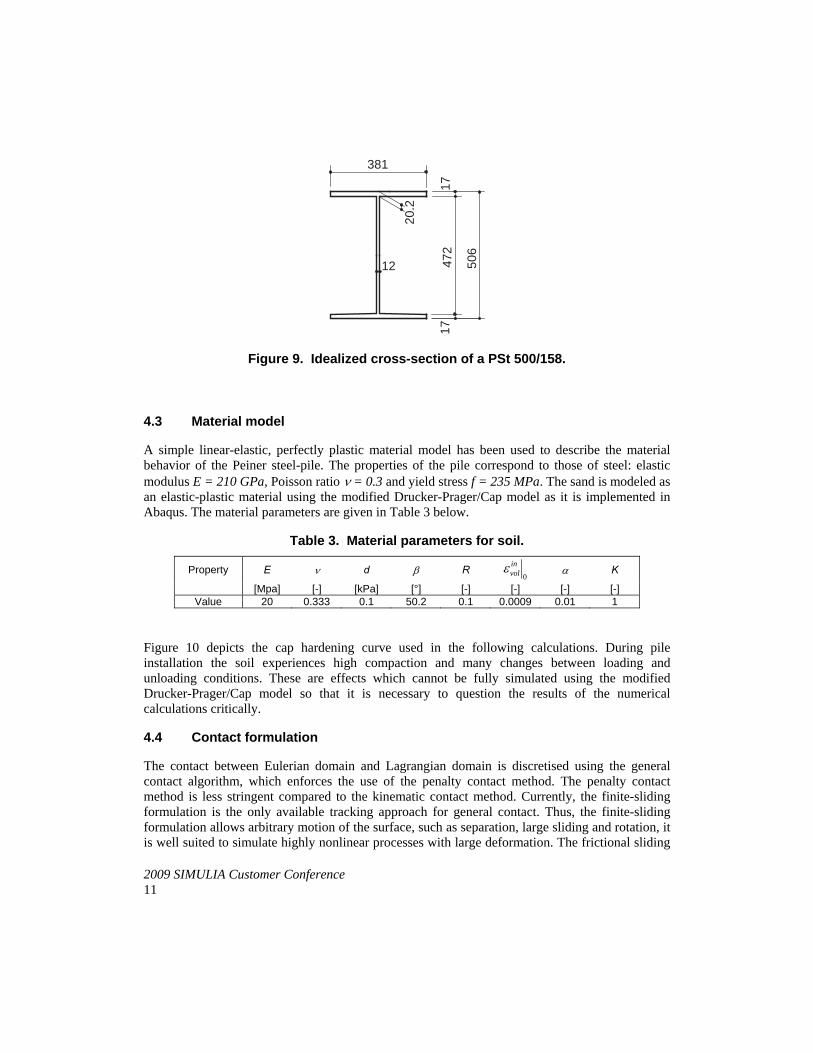
Figure 9. Idealized cross-section of a PSt 500/158.

4.3 Material model

A simple linear-elastic, perfectly plastic material model has been used to describe the material behavior of the Peiner steel-pile. The properties of the pile correspond to those of steel: elastic modulus E = 210 GPa, Poisson ratio = 0.3 and yield stress f = 235 MPa. The sand is modeled as an elastic-plastic material using the modified Drucker-Prager/Cap model as it is implemented in Abaqus. The material parameters are given in Table 3 below.

Table 3. Material parameters for soil.

Property E d R 0

invol K

[Mpa] [-] [kPa] [°] [-] [-] [-] [-] Value 20 0.333 0.1 50.2 0.1 0.0009 0.01 1

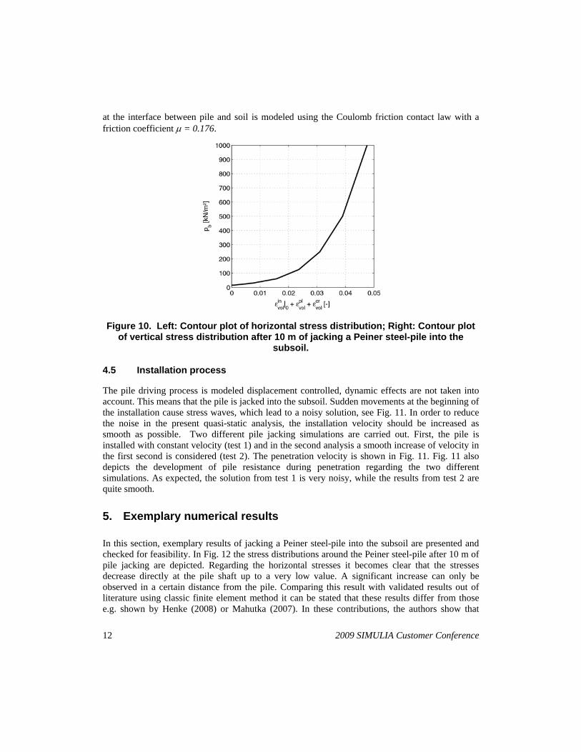
Figure 10 depicts the cap hardening curve used in the following calculations. During pile installation the soil experiences high compaction and many changes between loading and unloading conditions. These are effects which cannot be fully simulated using the modified Drucker-Prager/Cap model so that it is necessary to question the results of the numerical calculations critically.

4.4 Contact formulation

The contact between Eulerian domain and Lagrangian domain is discretised using the general contact algorithm, which enforces the use of the penalty contact method. The penalty contact method is less stringent compared to the kinematic contact method. Currently, the finite-sliding formulation is the only available tracking approach for general contact. Thus, the finite-sliding formulation allows arbitrary motion of the surface, such as separation, large sliding and rotation, it is well suited to simulate highly nonlinear processes with large deformation. The frictional sliding


at the interface between pile and soil is modeled using the Coulomb friction contact law with a friction coefficient = 0.176.

Figure 10. Left: Contour plot of horizontal stress distribution; Right: Contour plot of vertical stress distribution after 10 m of jacking a Peiner steel-pile into the

subsoil.

4.5 Installation process

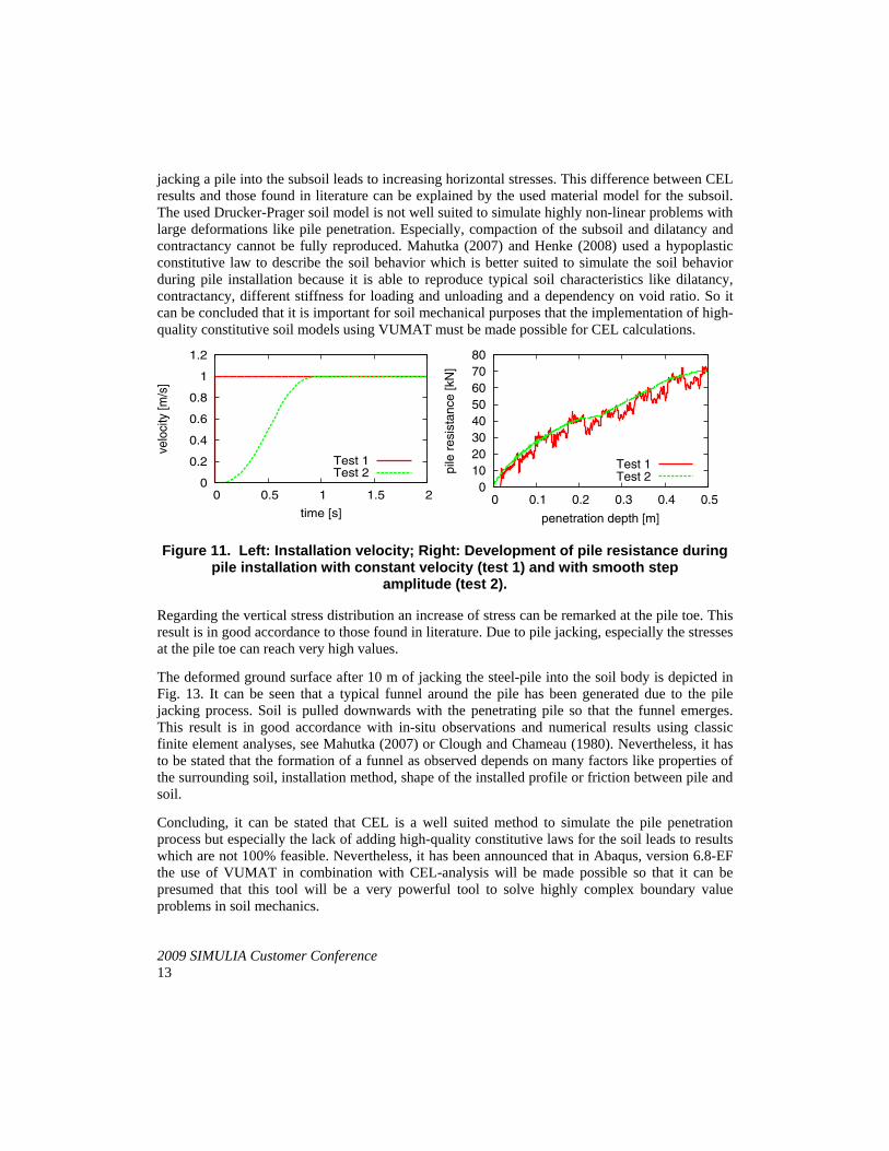
The pile driving process is modeled displacement controlled, dynamic effects are not taken into account. This means that the pile is jacked into the subsoil. Sudden movements at the beginning of the installation cause stress waves, which lead to a noisy solution, see Fig. 11. In order to reduce the noise in the present quasi-static analysis, the installation velocity should be increased as smooth as possible. Two different pile jacking simulations are carried out. First, the pile is installed with constant velocity (test 1) and in the second analysis a smooth increase of velocity in the first second is considered (test 2). The penetration velocity is shown in Fig. 11. Fig. 11 also depicts the development of pile resistance during penetration regarding the two different simulations. As expected, the solution from test 1 is very noisy, while the results from test 2 are quite smooth.

5. Exemplary numerical results

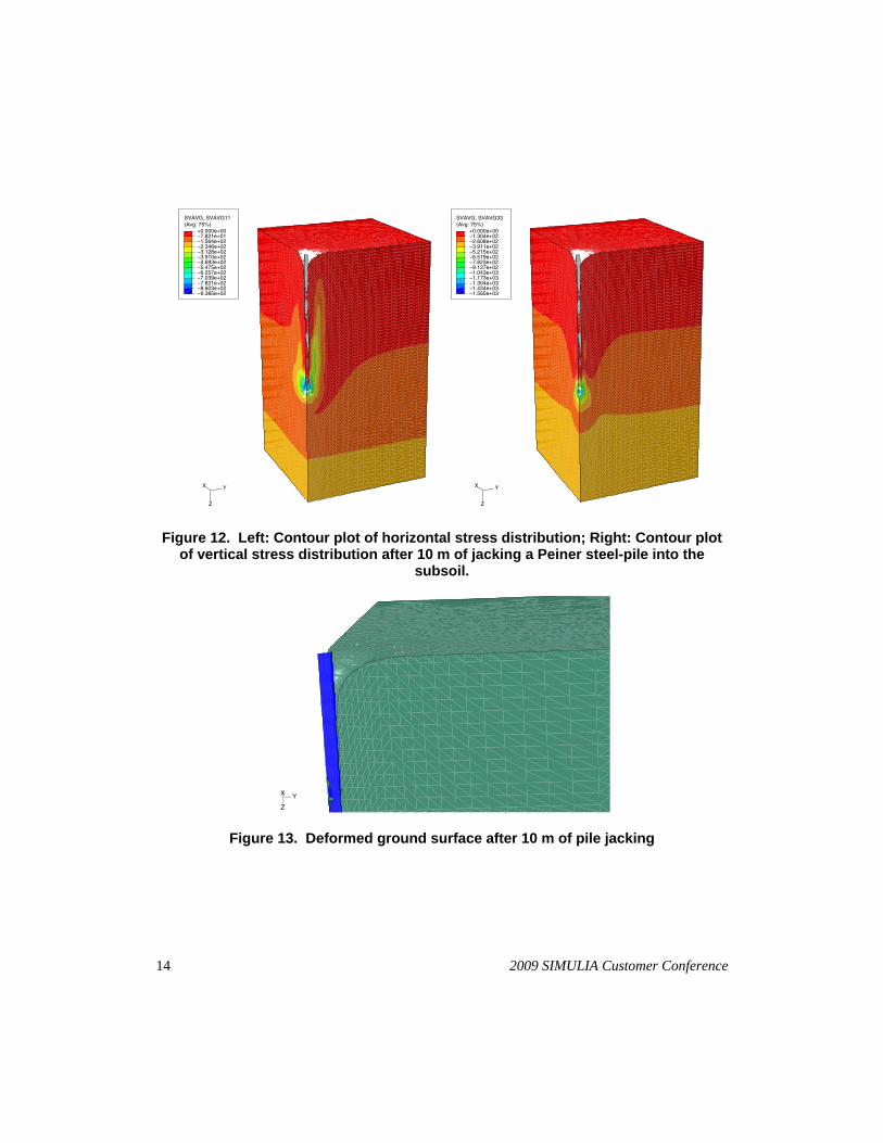
In this section, exemplary results of jacking a Peiner steel-pile into the subsoil are presented and checked for feasibility. In Fig. 12 the stress distributions around the Peiner steel-pile after 10 m of pile jacking are depicted. Regarding the horizontal stresses it becomes clear that the stresses decrease directly at the pile shaft up to a very low value. A significant increase can only be observed in a certain distance from the pile. Comparing this result with validated results out of literature using classic finite element method it can be stated that these results differ from those e.g. shown by Henke (2008) or Mahutka (2007). In these contributions, the authors show that


jacking a pile into the subsoil leads to increasing horizontal stresses. This difference between CEL results and those found in literature can be explained by the used material model for the subsoil. The used Drucker-Prager soil model is not well suited to simulate highly non-linear problems with large deformations like pile penetration. Especially, compaction of the subsoil and dilatancy and contractancy cannot be fully reproduced. Mahutka (2007) and Henke (2008) used a hypoplastic constitutive law to describe the soil behavior which is better suited to simulate the soil behavior during pile installation because it is able to reproduce typical soil characteristics like dilatancy, contractancy, different stiffness for loading and unloading and a dependency on void ratio. So it can be concluded that it is important for soil mechanical purposes that the implementation of high-quality constitutive soil models using VUMAT must be made possible for CEL calculations.

0

0.2

0.4

0.6

0.8

1

1.2

0 0.5 1 1.5 2

velo

city

[m/s

]

time [s]

Test 1Test 2

0 10 20 30 40 50 60 70 80

0 0.1 0.2 0.3 0.4 0.5

pile

res

ista

nce

[kN

]

penetration depth [m]

Test 1Test 2

Figure 11. Left: Installation velocity; Right: Development of pile resistance during pile installation with constant velocity (test 1) and with smooth step

amplitude (test 2).

Regarding the vertical stress distribution an increase of stress can be remarked at the pile toe. This result is in good accordance to those found in literature. Due to pile jacking, especially the stresses at the pile toe can reach very high values.

The deformed ground surface after 10 m of jacking the steel-pile into the soil body is depicted in Fig. 13. It can be seen that a typical funnel around the pile has been generated due to the pile jacking process. Soil is pulled downwards with the penetrating pile so that the funnel emerges. This result is in good accordance with in-situ observations and numerical results using classic finite element analyses, see Mahutka (2007) or Clough and Chameau (1980). Nevertheless, it has to be stated that the formation of a funnel as observed depends on many factors like properties of the surrounding soil, installation method, shape of the installed profile or friction between pile and soil.

Concluding, it can be stated that CEL is a well suited method to simulate the pile penetration process but especially the lack of adding high-quality constitutive laws for the soil leads to results which are not 100% feasible. Nevertheless, it has been announced that in Abaqus, version 6.8-EF the use of VUMAT in combination with CEL-analysis will be made possible so that it can be presumed that this tool will be a very powerful tool to solve highly complex boundary value problems in soil mechanics.


(Avg: 75%)SVAVG, SVAVG11

−9.385e+02−8.603e+02−7.821e+02−7.039e+02−6.257e+02−5.475e+02−4.693e+02−3.910e+02−3.128e+02−2.346e+02−1.564e+02−7.821e+01+0.000e+00

X Y

Z

(Avg: 75%)SVAVG, SVAVG33

−1.565e+03−1.434e+03−1.304e+03−1.173e+03−1.043e+03−9.127e+02−7.823e+02−6.519e+02−5.215e+02−3.911e+02−2.608e+02−1.304e+02+0.000e+00

X Y

Z

Figure 12. Left: Contour plot of horizontal stress distribution; Right: Contour plot of vertical stress distribution after 10 m of jacking a Peiner steel-pile into the

subsoil.

X Y

Z

Figure 13. Deformed ground surface after 10 m of pile jacking


6. Conclusion and outlook

According to two benchmark problems it can be concluded that the CEL-method is well suited to solve geotechnical problems with large deformations of the soil body and the interacting structure. Solving soil-structure-interaction problems singular plasticity points often can be found at the edge of the structures. The free deformable soil in an Eulerian domain can overcome the effect of singular plasticity points automatically. Due to large deformations of the structure a clearance between soil and structure can occur. This leads to non-linearities at the boundary and can induce convergence problems if an implicit analysis is chosen. Regarding the two investigated benchmark problems it can be stated that only CEL-method is able to predict the resulting loads at limit state correctly because the Eulerian mesh is not restricted by mesh or element distortions.

Furthermore, an example of simulating pile penetration into the subsoil is shown to show the capabilities of CEL to simulate complex geotechnical problems involving large deformations. It can be stated that CEL is well suited to simulate the pile penetration process without the limitations of a classical finite element formulation.

Nevertheless, there are some features that have to be improved. Especially, it is necessary for soil mechanical purposes that user subroutines (esp. VUMAT) are made available for Eulerian domains. Soil is a complex material which cannot be described correctly using the Abaqus’ built-in constitutive models. Especially, if complex boundary value problems involving large deformations and/or dynamic effects have to be solved, high-quality constitutive models are necessary.

If the use of VUMAT in combination with CEL is made possible, CEL is expected to be a very powerful tool to deal with geotechnical boundary value problems, which are nowadays hardly solvable using finite element method.

7. References

1. Chopra, M.B., Dargush, G.F., Finite-Element Analysis of time-dependant large-deformations Problems. International Journal for Numerical and Analytical Methods in Geomechanics 16, 101-130, 1992.

2. Clough, G.W., Chameau, J.-L., Measured Effects of Vibratory Sheetpile Driving. Journal of Geotechnical Engineering Division, 106(10): 1081-1099, 1980.

3. Cudmani, R.O., Statische, alternierende und dynamische Penetration in nichtbindigen Böden. Dissertation. Veröffentlichungen des Institutes für Bodenmechanik und Felsmechanik der Universität Fridericiana in Karlsruhe, Heft 152, 2001.

4. Henke, S., Grabe, J., Simulation of pile driving by 3-dimensional Finite-Element analysis. Proceedings of 17th European Young Geotechnical Engineers’ Conference, Zagreb, pp.215-233, 2006.

5. Henke, S., Hügel, H.M., Räumliche Analysen zur quasi-statischen und dynamischen Penetration von Bauteilen in den Untergrund. Tagungsband zur 19. deutschen Abaqus-Benutzerkonferenz in Baden-Baden, Artikel 2.13, 2007.


6. Henke, S., Herstellungseinflüsse aus Pfahlrammung im Kaimauerbau. Dissertation. Veröffentlichungen des Instituts für Geotechnik und Baubetrieb der Technischen Universität Hamburg-Harburg, Heft 18, 2008.

7. Hill, R., “The Mathematical Theory of Plasticity,” Oxford, 1950.

8. van Langen, H., “Numerical analysis of soil-structure interaction ,” Ph.D. Thesis, Delft University of Technology, 1991.

9. Mabsout, M.E., Tassoulas, J.L., A finite element model for the simulation of pile driving. International Journal for Numerical and Analytical Methods in Geomechanics, 37, 257-278, 1994.

10. Mahutka, K.-P., König, F., Grabe, J., Numerical modeling of pile jacking, driving and vibro driving. Proceedings of International Conference on Numerical Simulations of Construction Processes in Geotechnical Engineering for Urban Environment (NSC06), Bochum, pp. 235-246, 2006.

11. Mahutka, K.-P., Zur Verdichtung von rolligen Böden infolge dynamischer Pfahleinbringung und durch Oberflächenrüttler. Dissertation. Veröffentlichungen des Instituts für Geotechnik und Baubetrieb der Technischen Universität Hamburg-Harburg, Heft 15, 2007.

12. Mardfeldt, B., “Verformungsverhalten von Kaimauerkonstruktionen im Gebrauchszustand”, Promotionsschrift, Veröffentlichungen des Instituts für Geotechnik und Baubetrieb der Technische Universität Hamburg-Harburg, Heft 11, 2005.

Acknowledgement

The authors thank the German Research Foundation (DFG) for funding the present project in the framework of the post-graduate programme “Seaports for container ships of future generations”.

applications of coupled eulerian-lagrangian method to ... · pdf fileapplications of coupled...

Documents