arbitrary lagrangian-eulerian simulations of a...
TRANSCRIPT
Bag plate Bag plate
Bag
Pressure tank Nozzle
Pressure pulse
Dust
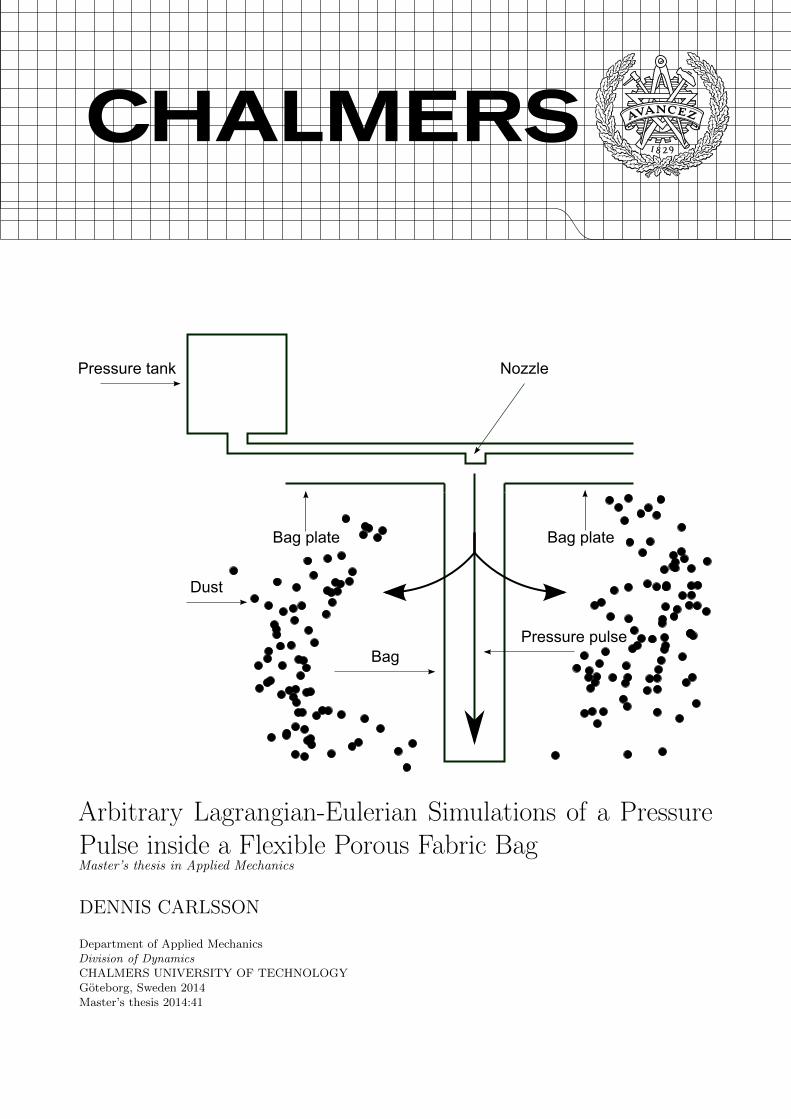
Arbitrary Lagrangian-Eulerian Simulations of a PressurePulse inside a Flexible Porous Fabric BagMaster’s thesis in Applied Mechanics
DENNIS CARLSSON
Department of Applied MechanicsDivision of DynamicsCHALMERS UNIVERSITY OF TECHNOLOGYGoteborg, Sweden 2014Master’s thesis 2014:41

MASTER’S THESIS IN APPLIED MECHANICS
Arbitrary Lagrangian-Eulerian Simulations of a Pressure Pulse inside aFlexible Porous Fabric Bag
DENNIS CARLSSON
Department of Applied MechanicsDivision of Dynamics
CHALMERS UNIVERSITY OF TECHNOLOGY
Goteborg, Sweden 2014
Arbitrary Lagrangian-Eulerian Simulations of a Pressure Pulse inside a Flexible Porous Fabric BagDENNIS CARLSSON
c© DENNIS CARLSSON, 2014
Master’s thesis 2014:41ISSN 1652-8557Department of Applied MechanicsDivision of DynamicsChalmers University of TechnologySE-412 96 GoteborgSwedenTelephone: +46 (0)31-772 1000
Cover:A pressure pulse is injected inside a fabric bag to remove dust from the bag surface
Chalmers ReproserviceGoteborg, Sweden 2014
Arbitrary Lagrangian-Eulerian Simulations of a Pressure Pulse inside a Flexible Porous Fabric BagMaster’s thesis in Applied MechanicsDENNIS CARLSSONDepartment of Applied MechanicsDivision of DynamicsChalmers University of Technology
Abstract
In today’s society, combustion processes are important for heat and power generation. A negative effect of thecombustion processes are the increase of emissions in the air which can affect the environment and humanhealth in a negative manner. To reduce emissions and increase air quality, Air Quality Control Systems (AQCS)can be used. There are different kinds of AQCS but in this thesis the focus is on fabric filters, which is anAQCS that reduce the amount of particles and dust in the air. In a fabric filter there are hundreds of fabricbags, hanging in the ceiling of the filter. The air is flowing through the bag and the dust gets stuck on thesurface of the bag. When the bag gets covered by dust, the filtering effect decrease and the bag needs to becleaned. The cleaning of a bag is done by a powerful pressure pulse on the inside of the bag. The pressurepulse gives the bag an acceleration, which removes the dust from the bag. In this thesis a parameter study wasmade to see how the acceleration was affected by different parameters. The considered parameters were thepermeability of the bag and the weight of the dust on the bag surface and these were compared to a referencecase representing a clean bag. There existed experimental results that were compared to the simulation results.
The cleaning of a bag was modelled in LS-DYNA using the Arbitrary Lagrangian-Eulerian (ALE) approachwith a fluid-structure interaction between the bag and the air. Unfortunately, the pressure propagated muchslower in the simulations compared to the experiments and also the magnitude of the pressure pulse was tolow. The reason for this was probably due to the boundary condition defining the pressure pulse. Even if thepressure was not accurate in all respects, the acceleration of the bag was investigated to see if any trends ofhow the bag was affected by the different parameters could be found. Unfortunately, an uneven distribution ofinitial deformation (also called slack), made it hard to predict some aspects regarding the acceleration due tothat the acceleration differed a lot between different points at the same height on the bag. To be able to usethis kind of simulations to improve the cleaning of a bag, the pressure pulse needs to be defined in such a wayso that it get a better agreement with the experimental result. Also a method about how the accelerationsshould be measured needs to be investigated.
Keywords: Arbitrary Lagrangian-Eulerian, ALE, Fluid-Structure Interaction, FSI, Fabrics, Porous
i

ii
Preface
In this study, the possibilities to model the dynamics of a fabric bag resulting from a pressure pulse duringcleaning were investigated. The thesis was made during January to June 2014 at ALSTOM POWER SWEDENAB in Vaxjo. I want to thank my supervisor at ALSTOM, Micko Bjorck, for his dedication and help during thisthesis. I also want to thank Robert Moestam and Lars-Erik Johansson at the ALSTOM laboratory for providingme with experimental data and tips about the modelling approach. Also a thank to Matthias Kirchhoff atBWF Envirotec in Offingen, Germany for providing me with material data for the fabric bag. A special thanksto Livermore Software Technology Corporation (LSTC) in Livermore, CA, United States for providing mewith free licenses to the finite element program LS-DYNA, which have been used in this thesis. I also want tothank my examiner at the department of Applied Mechanics, division of Dynamics at Chalmers Univeristy ofTechnology, Peter Folkow, for support during the thesis. Also a thank to Karin Brolin for help with LS-DYNArelated questions.
Vaxjo, June 2014Dennis Carlsson
iii

iv

Nomenclature
Roman Symbols
Symbol DescriptionAn Ergun’s viscous coefficientBn Ergun’s inertial coefficientCp Specific heat at constant pressureCv Specific heat at constant volumed Penetrating distanceDijkl Stiffness tensore Total internal energy per unit massEij Green-Lagrange strain tensorFi Force vectorFij Deformation gradiente0 Total initial energy per unit massI0 MomentumIij Moment of inertia tensorks Contact stiffnessLi Angular momentum vector around center of gravitym MassMi Moment vector around center of gravityni Normal vectorp Pressurep0 Total pressureR Gas constantt Time or thickness∆tcr Critical time step sizeT Temperatureui Displacement vectorvi Velocity vectorvi Mesh velocity vectorvn Relative velocityW Energy/Workxi Spatial coordinate vectorXj Reference position vector
Greek Symbols
Symbol Descriptionγ Ratio of the specific heatsδij Kronecker’s delta functionε Porosityε′ij Strain rate tensorµ Dynamic viscosityρ Densityσij Cauchy stress tensorσ′ij Deviatoric Cauchy stress tensorφ Transport quantityωi Angular velocity vectorωmax Highest eigenfrequency
Abbreviations
ALE Arbitrary Lagrangian-EulerianAQCS Air Quality Control SystemsFEM Finite Element MethodFSI Fluid Structure InteractionLSTC Livermore Software Technology CorporationMMALE Multi Material Arbitrary Lagrangian-Eulerian
v

vi
Contents
Abstract i
Preface iii
Nomenclature v
Contents vii
1 Introduction 11.1 Background . . . . . . . . . . . . . . . . . . . . . . . . . . . . . . . . . . . . . . . . . . . . . . . . . 31.2 Purpose and problem description . . . . . . . . . . . . . . . . . . . . . . . . . . . . . . . . . . . . . 41.3 Delimitations . . . . . . . . . . . . . . . . . . . . . . . . . . . . . . . . . . . . . . . . . . . . . . . . 4
2 Theory 52.1 Arbitrary Lagrangian-Eulerian simulations . . . . . . . . . . . . . . . . . . . . . . . . . . . . . . . . 52.1.1 Lagrangian and Eulerian formulation . . . . . . . . . . . . . . . . . . . . . . . . . . . . . . . . . 52.1.2 Multi Material Arbitrary Lagrangian-Eulerian description . . . . . . . . . . . . . . . . . . . . . . 52.2 Solid bodies . . . . . . . . . . . . . . . . . . . . . . . . . . . . . . . . . . . . . . . . . . . . . . . . . 62.3 Fluid-structure interaction . . . . . . . . . . . . . . . . . . . . . . . . . . . . . . . . . . . . . . . . . 72.3.1 Constrained based coupling . . . . . . . . . . . . . . . . . . . . . . . . . . . . . . . . . . . . . . . 72.3.2 Penalty based coupling . . . . . . . . . . . . . . . . . . . . . . . . . . . . . . . . . . . . . . . . . 82.4 Advection algorithms . . . . . . . . . . . . . . . . . . . . . . . . . . . . . . . . . . . . . . . . . . . 82.4.1 Donor Cell algorithm . . . . . . . . . . . . . . . . . . . . . . . . . . . . . . . . . . . . . . . . . . 92.4.2 Van Leer MUSCL scheme . . . . . . . . . . . . . . . . . . . . . . . . . . . . . . . . . . . . . . . . 92.5 Critical time step size . . . . . . . . . . . . . . . . . . . . . . . . . . . . . . . . . . . . . . . . . . . 102.6 Porosity and permeability . . . . . . . . . . . . . . . . . . . . . . . . . . . . . . . . . . . . . . . . . 112.7 Total and static pressure . . . . . . . . . . . . . . . . . . . . . . . . . . . . . . . . . . . . . . . . . . 112.8 Artificial bulk viscosity . . . . . . . . . . . . . . . . . . . . . . . . . . . . . . . . . . . . . . . . . . 12
3 Simulation set-up 133.1 Geometry and model dimensions . . . . . . . . . . . . . . . . . . . . . . . . . . . . . . . . . . . . . 133.2 Part modelling . . . . . . . . . . . . . . . . . . . . . . . . . . . . . . . . . . . . . . . . . . . . . . . 153.3 Boundary conditions and loads . . . . . . . . . . . . . . . . . . . . . . . . . . . . . . . . . . . . . . 163.4 Contact definitions . . . . . . . . . . . . . . . . . . . . . . . . . . . . . . . . . . . . . . . . . . . . . 183.5 Cases . . . . . . . . . . . . . . . . . . . . . . . . . . . . . . . . . . . . . . . . . . . . . . . . . . . . 183.5.1 Reference case . . . . . . . . . . . . . . . . . . . . . . . . . . . . . . . . . . . . . . . . . . . . . . 193.5.2 Other cases . . . . . . . . . . . . . . . . . . . . . . . . . . . . . . . . . . . . . . . . . . . . . . . . 19
4 Result 214.1 Comparison with experiments . . . . . . . . . . . . . . . . . . . . . . . . . . . . . . . . . . . . . . . 214.1.1 Mass of the inflowing air into a bag . . . . . . . . . . . . . . . . . . . . . . . . . . . . . . . . . . 214.1.2 Pressure at the bag surface . . . . . . . . . . . . . . . . . . . . . . . . . . . . . . . . . . . . . . . 224.2 Reference case . . . . . . . . . . . . . . . . . . . . . . . . . . . . . . . . . . . . . . . . . . . . . . . 274.2.1 Flow characteristics . . . . . . . . . . . . . . . . . . . . . . . . . . . . . . . . . . . . . . . . . . . 274.2.2 Bag dynamics . . . . . . . . . . . . . . . . . . . . . . . . . . . . . . . . . . . . . . . . . . . . . . . 344.3 Cases with different permeability . . . . . . . . . . . . . . . . . . . . . . . . . . . . . . . . . . . . . 404.4 Case with different dust cake weight . . . . . . . . . . . . . . . . . . . . . . . . . . . . . . . . . . . 40
5 Discussion 445.1 Future work . . . . . . . . . . . . . . . . . . . . . . . . . . . . . . . . . . . . . . . . . . . . . . . . . 45
6 Conclusions 46
References 47
vii
A Index notation and Einstein convention I
B Proof of symmetric stress tensor II
C Keyword input commands IV
viii
1 Introduction
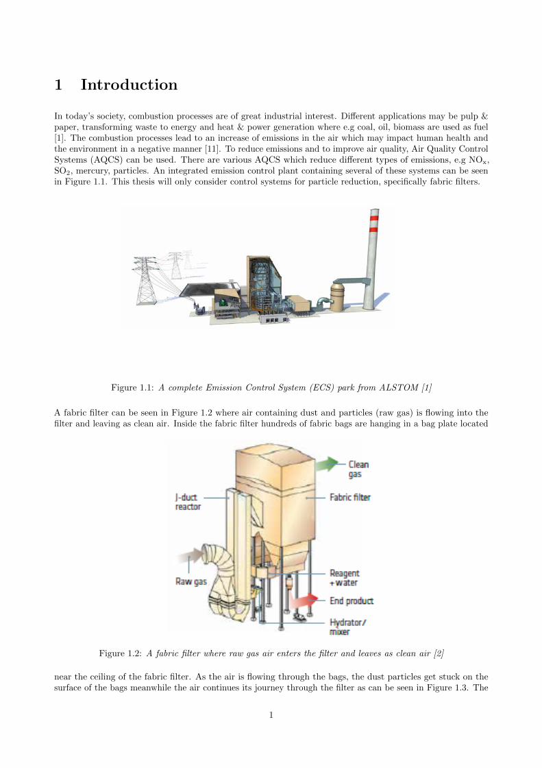
In today’s society, combustion processes are of great industrial interest. Different applications may be pulp &paper, transforming waste to energy and heat & power generation where e.g coal, oil, biomass are used as fuel[1]. The combustion processes lead to an increase of emissions in the air which may impact human health andthe environment in a negative manner [11]. To reduce emissions and to improve air quality, Air Quality ControlSystems (AQCS) can be used. There are various AQCS which reduce different types of emissions, e.g NOx,SO2, mercury, particles. An integrated emission control plant containing several of these systems can be seenin Figure 1.1. This thesis will only consider control systems for particle reduction, specifically fabric filters.
Figure 1.1: A complete Emission Control System (ECS) park from ALSTOM [1]
A fabric filter can be seen in Figure 1.2 where air containing dust and particles (raw gas) is flowing into thefilter and leaving as clean air. Inside the fabric filter hundreds of fabric bags are hanging in a bag plate located
Figure 1.2: A fabric filter where raw gas air enters the filter and leaves as clean air [2]
near the ceiling of the fabric filter. As the air is flowing through the bags, the dust particles get stuck on thesurface of the bags meanwhile the air continues its journey through the filter as can be seen in Figure 1.3. The
1
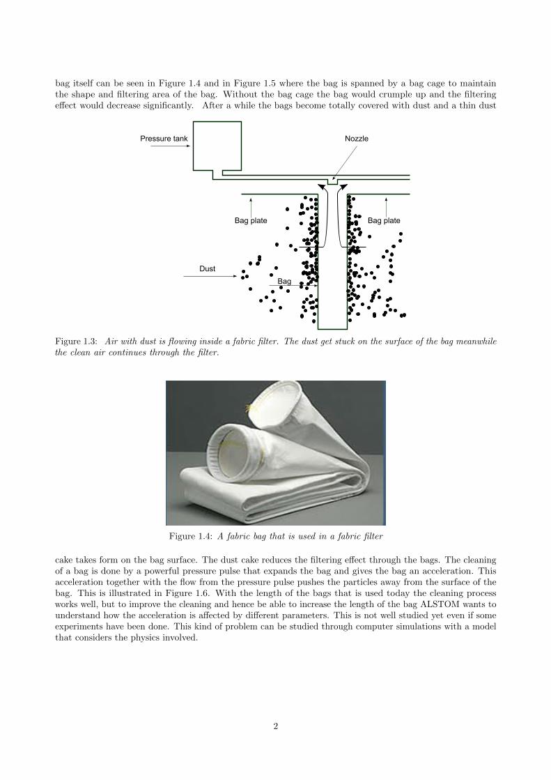
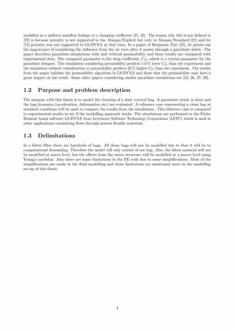
bag itself can be seen in Figure 1.4 and in Figure 1.5 where the bag is spanned by a bag cage to maintainthe shape and filtering area of the bag. Without the bag cage the bag would crumple up and the filteringeffect would decrease significantly. After a while the bags become totally covered with dust and a thin dust
Bag plate Bag plate
Bag
Pressure tank Nozzle
Dust
Figure 1.3: Air with dust is flowing inside a fabric filter. The dust get stuck on the surface of the bag meanwhilethe clean air continues through the filter.
Figure 1.4: A fabric bag that is used in a fabric filter
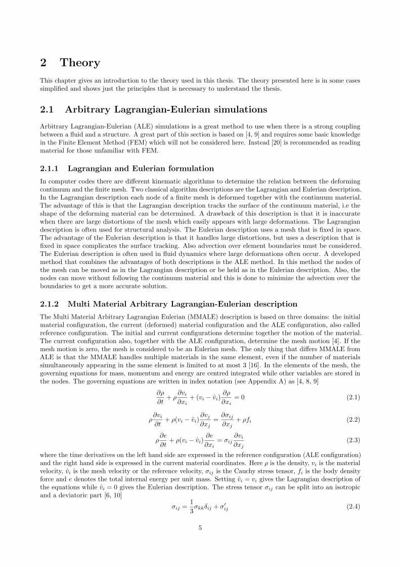
cake takes form on the bag surface. The dust cake reduces the filtering effect through the bags. The cleaningof a bag is done by a powerful pressure pulse that expands the bag and gives the bag an acceleration. Thisacceleration together with the flow from the pressure pulse pushes the particles away from the surface of thebag. This is illustrated in Figure 1.6. With the length of the bags that is used today the cleaning processworks well, but to improve the cleaning and hence be able to increase the length of the bag ALSTOM wants tounderstand how the acceleration is affected by different parameters. This is not well studied yet even if someexperiments have been done. This kind of problem can be studied through computer simulations with a modelthat considers the physics involved.
2
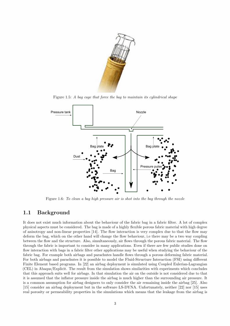
Figure 1.5: A bag cage that force the bag to maintain its cylindrical shape
Bag plate Bag plate
Bag
Pressure tank Nozzle
Pressure pulse
Dust
Figure 1.6: To clean a bag high pressure air is shot into the bag through the nozzle
1.1 Background
It does not exist much information about the behaviour of the fabric bag in a fabric filter. A lot of complexphysical aspects must be considered. The bag is made of a highly flexible porous fabric material with high degreeof anisotropy and non-linear properties [14]. The flow interaction is very complex due to that the flow maydeform the bag, which on the other hand will change the flow behaviour, i.e there may be a two way couplingbetween the flow and the structure. Also, simultaneously, air flows through the porous fabric material. The flowthrough the fabric is important to consider in many applications. Even if there are few public studies done onflow interaction with bags in a fabric filter other applications may be useful when studying the behaviour of thefabric bag. For example both airbags and parachutes handle flows through a porous deforming fabric material.For both airbags and parachutes it is possible to model the Fluid-Structure Interaction (FSI) using differentFinite Element based programs. In [22] an airbag deployment is simulated using Coupled Eulerian-Lagrangian(CEL) in Abaqus/Explicit. The result from the simulation shows similarities with experiments which concludesthat this approach suits well for airbags. In that simulation the air on the outside is not considered due to thatit is assumed that the inflator pressure inside the airbag is much higher than the surrounding air pressure. Itis a common assumption for airbag designers to only consider the air remaining inside the airbag [25]. Also[15] consider an airbag deployment but in the software LS-DYNA. Unfortunately, neither [22] nor [15] usesreal porosity or permeability properties in the simulations which means that the leakage from the airbag is
3
modelled as a uniform massflow leakage or a damping coefficient [21, 25]. The reason why this is not defined in[22] is because porosity is not supported in the Abaqus/Explicit but only in Abaqus/Standard [21] and for[15] porosity was not supported in LS-DYNA at that time. In a paper of Benjamin Tutt [25], he points outthe importance of considering the influence from the air even after it passes through a parachute fabric. Thepaper describes parachute simulations with and without permeability and these results are compared withexperimental data. The compared parameter is the drag coefficient, CD, which is a crucial parameter for theparachute designer. The simulation considering permeability predicts 1.6 % lower CD than the experiment andthe simulation without consideration to permeability predicts 25 % higher CD than the experiment. The resultsfrom the paper validate the permeability algorithm in LS-DYNA and show that the permeability may have agreat impact on the result. Some other papers considering similar parachute simulations are [24, 26, 27, 29].
1.2 Purpose and problem description
The purpose with this thesis is to model the cleaning of a dust covered bag. A parameter study is done andthe bag dynamics (acceleration, deformation etc) are evaluated. A reference case representing a clean bag atstandard conditions will be used to compare the results from the simulations. This reference case is comparedto experimental results to see if the modelling approach works. The simulations are performed in the FiniteElement based software LS-DYNA from Livermore Software Technology Corporation (LSTC) which is used inother applications considering flows through porous flexible materials.
1.3 Delimitations
In a fabric filter there are hundreds of bags. All these bags will not be modelled due to that it will be tocomputational demanding. Therefore the model will only consist of one bag. Also, the fabric material will notbe modelled at micro level, but the effects from the micro structure will be modelled at a macro level usingYoung’s modulus. Also there are some limitations in the FE code due to some simplifications. Most of thesimplifications are made in the fluid modelling and those limitations are mentioned more in the modellingset-up of this thesis.
4
2 Theory
This chapter gives an introduction to the theory used in this thesis. The theory presented here is in some casessimplified and shows just the principles that is necessary to understand the thesis.
2.1 Arbitrary Lagrangian-Eulerian simulations
Arbitrary Lagrangian-Eulerian (ALE) simulations is a great method to use when there is a strong couplingbetween a fluid and a structure. A great part of this section is based on [4, 9] and requires some basic knowledgein the Finite Element Method (FEM) which will not be considered here. Instead [20] is recommended as readingmaterial for those unfamiliar with FEM.
2.1.1 Lagrangian and Eulerian formulation
In computer codes there are different kinematic algorithms to determine the relation between the deformingcontinuum and the finite mesh. Two classical algorithm descriptions are the Lagrangian and Eulerian description.In the Lagrangian description each node of a finite mesh is deformed together with the continuum material.The advantage of this is that the Lagrangian description tracks the surface of the continuum material, i.e theshape of the deforming material can be determined. A drawback of this description is that it is inaccuratewhen there are large distortions of the mesh which easily appears with large deformations. The Lagrangiandescription is often used for structural analysis. The Eulerian description uses a mesh that is fixed in space.The advantage of the Eulerian description is that it handles large distortions, but uses a description that isfixed in space complicates the surface tracking. Also advection over element boundaries must be considered.The Eulerian description is often used in fluid dynamics where large deformations often occur. A developedmethod that combines the advantages of both descriptions is the ALE method. In this method the nodes ofthe mesh can be moved as in the Lagrangian description or be held as in the Eulerian description. Also, thenodes can move without following the continuum material and this is done to minimize the advection over theboundaries to get a more accurate solution.
2.1.2 Multi Material Arbitrary Lagrangian-Eulerian description
The Multi Material Arbitrary Lagrangian Eulerian (MMALE) description is based on three domains: the initialmaterial configuration, the current (deformed) material configuration and the ALE configuration, also calledreference configuration. The initial and current configurations determine together the motion of the material.The current configuration also, together with the ALE configuration, determine the mesh motion [4]. If themesh motion is zero, the mesh is considered to be an Eulerian mesh. The only thing that differs MMALE fromALE is that the MMALE handles multiple materials in the same element, even if the number of materialssimultaneously appearing in the same element is limited to at most 3 [16]. In the elements of the mesh, thegoverning equations for mass, momentum and energy are centred integrated while other variables are stored inthe nodes. The governing equations are written in index notation (see Appendix A) as [4, 8, 9]
∂ρ
∂t+ ρ
∂vi∂xi
+ (vi − vi)∂ρ
∂xi= 0 (2.1)
ρ∂vi∂t
+ ρ(vi − vi)∂vj∂xj
=∂σij∂xj
+ ρfi (2.2)
ρ∂e
∂t+ ρ(vi − vi)
∂e
∂xi= σij
∂vi∂xj
(2.3)
where the time derivatives on the left hand side are expressed in the reference configuration (ALE configuration)and the right hand side is expressed in the current material coordinates. Here ρ is the density, vi is the materialvelocity, vi is the mesh velocity or the reference velocity, σij is the Cauchy stress tensor, fi is the body densityforce and e denotes the total internal energy per unit mass. Setting vi = vi gives the Lagrangian description ofthe equations while vi = 0 gives the Eulerian description. The stress tensor σij can be split into an isotropicand a deviatoric part [6, 10]
σij =1
3σkkδij + σ′ij (2.4)
5
where δij is the Kroneckers delta function which equals unity if i = j and equals zero if i 6= j. This meansthat the first term in eq (2.4) is only active in the normal directions. As pressure p acts in negative normaldirection we conclude that σkk/3 = −p in eq (2.4) [6]. The deviatoric part σ′ij contains the shear stress and isdefined as [17]
σ′ij = 2µε′ij (2.5)
where µ is the dynamic viscosity and ε′ij is the strain rate tensor defined as
ε′ij =1
2
(∂vi∂xj
+∂vj∂xi
)(2.6)
Inserting all together, a final expression for the stress tensor is achieved
σij = −pδij + µ
(∂vi∂xj
+∂vj∂xi
)(2.7)
In the one dimensional case of the governing equations there are four unknown variables, ρ, vi=1, e and pbut there are only three equations. Therefore an extra equation is needed to close the system. The requiredequation is the equation of state which determine the pressure. The equation of state is dependent on theproblem type but for a gas the ideal gas law can be used
p = ρRT = ρ(Cp − Cv)T (2.8)
where ρ is the density, T is the temperature, Cp and Cv are the specific heat coefficients at constant pressureand constant volume, respectively. Using the ideal gas approach the initial energy per unit mass for the fluidis defined as e0 = CvT where the total initial energy per unit mass is defined as e = e0 + (1/2)vivi. In thethree dimensional case there are three velocity components vi, where i = 1, 2, 3 but there are also two extraequations for the momentum and together with the equation of state the system will be closed.
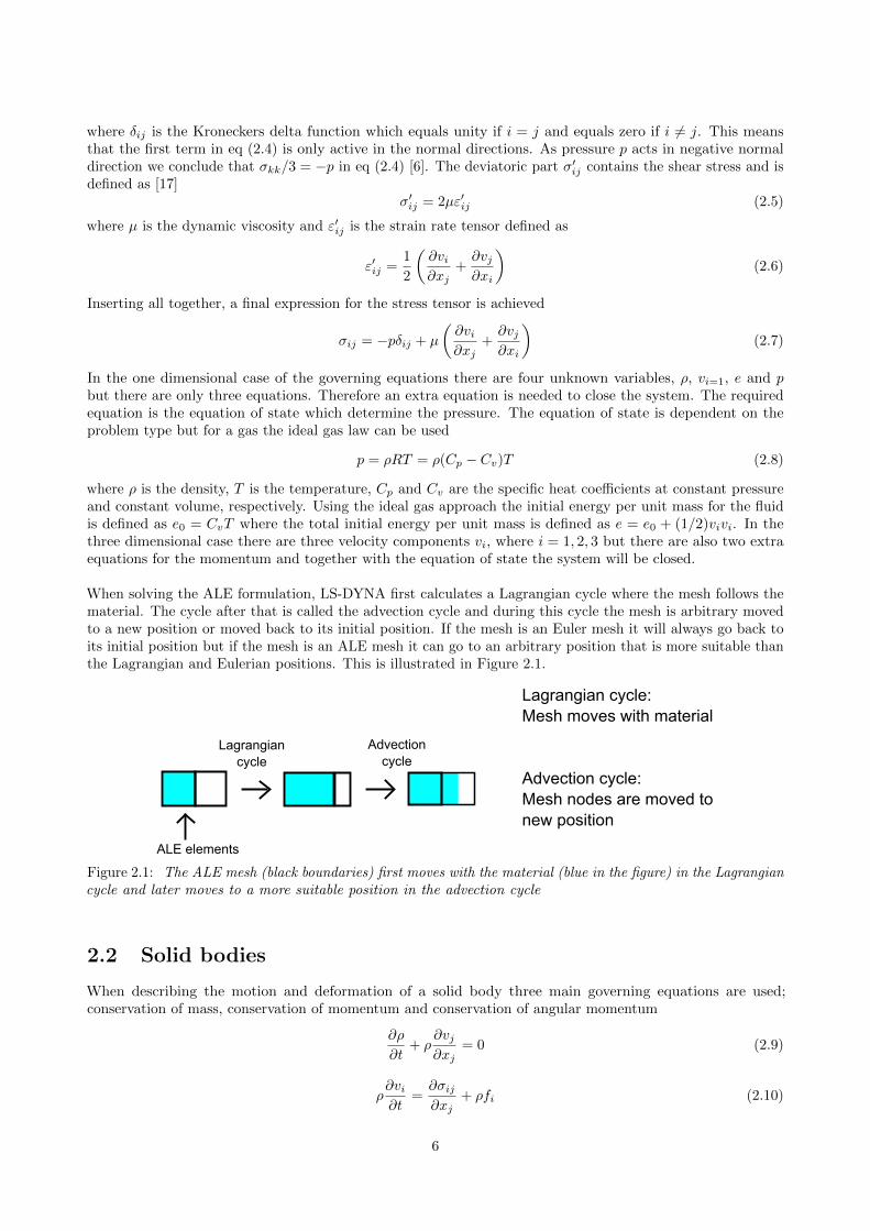
When solving the ALE formulation, LS-DYNA first calculates a Lagrangian cycle where the mesh follows thematerial. The cycle after that is called the advection cycle and during this cycle the mesh is arbitrary movedto a new position or moved back to its initial position. If the mesh is an Euler mesh it will always go back toits initial position but if the mesh is an ALE mesh it can go to an arbitrary position that is more suitable thanthe Lagrangian and Eulerian positions. This is illustrated in Figure 2.1.
Lagrangian
cycle
Advection
cycle
ALE elements
Lagrangian cycle:
Mesh moves with material
Advection cycle:
Mesh nodes are moved to
new position
Figure 2.1: The ALE mesh (black boundaries) first moves with the material (blue in the figure) in the Lagrangiancycle and later moves to a more suitable position in the advection cycle
2.2 Solid bodies
When describing the motion and deformation of a solid body three main governing equations are used;conservation of mass, conservation of momentum and conservation of angular momentum
∂ρ
∂t+ ρ
∂vj∂xj
= 0 (2.9)
ρ∂vi∂t
=∂σij∂xj
+ ρfi (2.10)
6
Mi = ˙Li where Li = Iijωj (2.11)
Equation (2.9) and (2.10) are the same as (2.1) and (2.2) in the ALE section but with the Lagrangian formulationinstead. In eq (2.11) Li is the angular momentum, Iij the moment of inertia, ωj angular velocity and Mi themoment [5]. A bar over a notation means that it is considered around the center of mass and a dot over anotation indicates time derivative. The conservation of angular momentum is used to prove symmetry of thestress tensor, σij = σji. The proof can be seen in Appendix B. This reduce the unknowns of σij from nine tosix components. Still there are more unknowns than equations and therefore the generalized Hooke’s law isused to express the stresses
σij = DijklEkl (2.12)
Here Dijkl is a forth order stiffness tensor and Ekl is the Green-Lagrange strain tensor which is used when largedeformations are present [23]. The Green-Lagrange strain tensor is defined by the deformation gradient Fij
Eij =1
2(FkiFkj − δij) (2.13)
Fij =∂xi∂Xj
(2.14)
where xi is the current position and Xj is the reference (undeformed) position. The displacement can beexpressed as
ui = xi −Xi (2.15)
Equation (2.14) and (2.15) into (2.13) gives a final expression for the Green-Lagrange strain as
Eij =1
2
(∂ui∂Xj
+∂uj∂Xi
+∂uk∂Xi
∂uk∂Xj
)(2.16)
If the body have small deformations the last term in eq (2.16) will be very small and the deformed and theundeformed reference location will almost coincide
Eij =1
2
(∂ui∂Xj
+∂uj∂Xi
)≈ 1
2
(∂ui∂xj
+∂uj∂xi
)= εij (2.17)
which means that for small deformations the Green-Lagrange strain can be approximated by the engineeringstrain εij .
2.3 Fluid-structure interaction
In many applications it is suitable to treat parts in different formulations. For example in fluid structureinteraction it is often a good choice to treat the fluid in Eulerian or ALE-formulation and the structure inLagrangian formulation. Therefore a coupling algorithm is needed for the different parts to communicate [19].For this coupling to work properly it is required that at least 2 or 3 coupling points per ALE element lengthare used during the whole simulation. These coupling points should be defined with care. In LS-DYNA thesepoints are defined on the Lagrangian segments which means that the user must consider the relative mesh sizebetween the Lagrangian and ALE mesh at the location of contact. Also too many coupling points may lead toinstabilities and too few lead to leakage [16]. Two methods for the coupling in LS-DYNA are the constrainedbased and the penalty based coupling. Both methods require that the ALE (or Eulerian) and the Lagrangianmesh overlap even if the nodes do not need to coincide [13].
2.3.1 Constrained based coupling
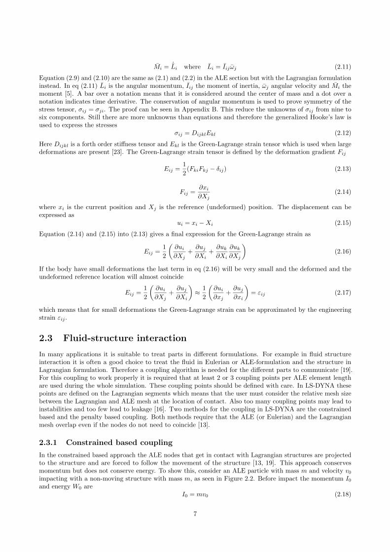
In the constrained based approach the ALE nodes that get in contact with Lagrangian structures are projectedto the structure and are forced to follow the movement of the structure [13, 19]. This approach conservesmomentum but does not conserve energy. To show this, consider an ALE particle with mass m and velocity v0
impacting with a non-moving structure with mass m, as seen in Figure 2.2. Before impact the momentum I0and energy W0 are
I0 = mv0 (2.18)
7
W0 =1
2mv2
0 (2.19)
When the ALE particle impacts the Lagrangian structure it get stuck on the Lagrangian structure. Themomentum is conserved during the impact which gives a velocity v1 = 1
2v0 for the system after the impactwhich can be concluded from eq (2.20). As a result of this new velocity the kinetic energy after the impact islower than before the impact which can be seen in eq (2.21).
I1 = (m+m)v1 = 2mv1 = I0 (2.20)
W1 =1
2(2m) (v1)
2=
1
2(2m)
(1
2v0
)2
=1
4mv2
0 < W0 (2.21)
Before impact After impact
m m m m
v0 v1 v1
a) b)
Figure 2.2: a) An ALE particle (left) is travelling ahead a non moving structure (right) b) After impacting thestructure, the ALE particle is moving together with the structure at the same speed
2.3.2 Penalty based coupling
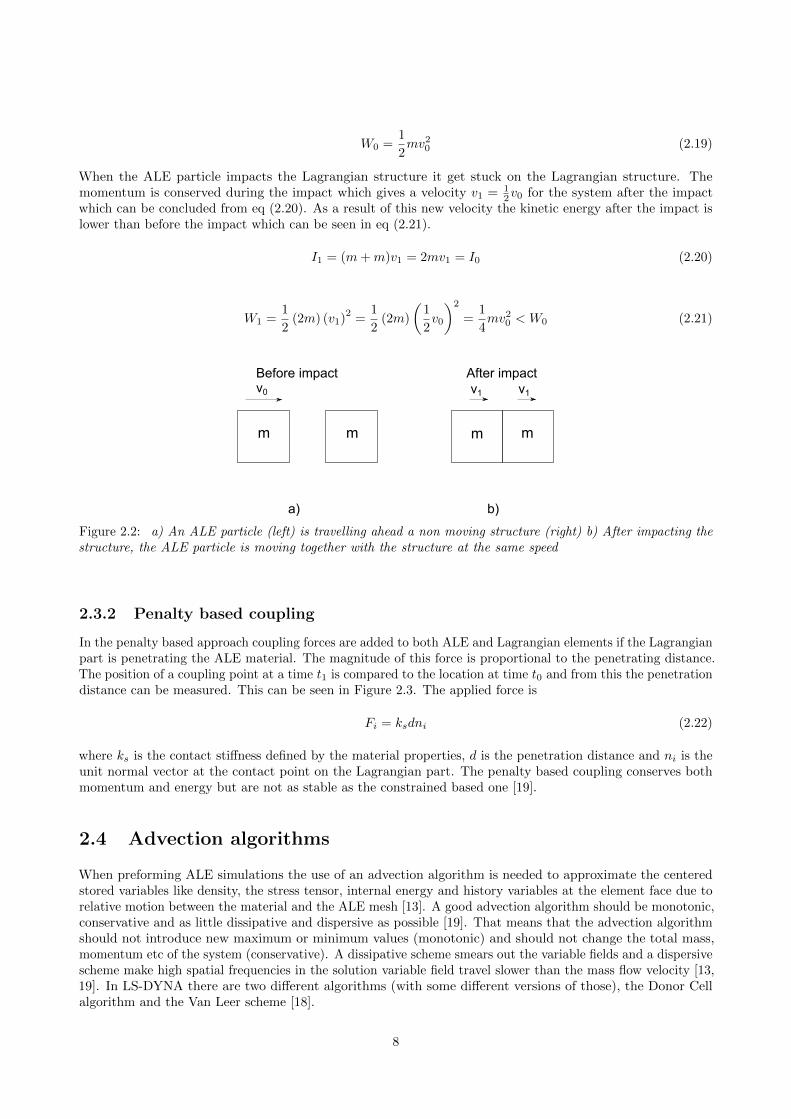
In the penalty based approach coupling forces are added to both ALE and Lagrangian elements if the Lagrangianpart is penetrating the ALE material. The magnitude of this force is proportional to the penetrating distance.The position of a coupling point at a time t1 is compared to the location at time t0 and from this the penetrationdistance can be measured. This can be seen in Figure 2.3. The applied force is
Fi = ksdni (2.22)
where ks is the contact stiffness defined by the material properties, d is the penetration distance and ni is theunit normal vector at the contact point on the Lagrangian part. The penalty based coupling conserves bothmomentum and energy but are not as stable as the constrained based one [19].
2.4 Advection algorithms
When preforming ALE simulations the use of an advection algorithm is needed to approximate the centeredstored variables like density, the stress tensor, internal energy and history variables at the element face due torelative motion between the material and the ALE mesh [13]. A good advection algorithm should be monotonic,conservative and as little dissipative and dispersive as possible [19]. That means that the advection algorithmshould not introduce new maximum or minimum values (monotonic) and should not change the total mass,momentum etc of the system (conservative). A dissipative scheme smears out the variable fields and a dispersivescheme make high spatial frequencies in the solution variable field travel slower than the mass flow velocity [13,19]. In LS-DYNA there are two different algorithms (with some different versions of those), the Donor Cellalgorithm and the Van Leer scheme [18].
8
d
a) b)
ALE
element
Lagrangian structure
At t=t0 At t=t1
coupling
point
Figure 2.3: a) Lagrangian structure penetrates an ALE element and the position of the coupling point at time t0is registered b) At time t1 the penetrating distance d can be measured from the updated position of the couplingpoint
2.4.1 Donor Cell algorithm
The Donor Cell Algorithm is a first order algorithm that is stable, monotonic and fast but it is also stronglydissipative and dispersive. However, due to the strong dissipation, the high frequencies that travel to slow arequickly damped out [19]. This limits the use of the Donor cell algorithm to fluids [19]. The one dimensionalDonor Cell Algorithm for a transport quantity, φ, between node j and j + 1, is
φn+1j+1/2 = φnj+1/2+
∆t
∆x(fφj − f
φj+1)
fφj =aj2
(φnj−1/2 + φnj+1/2)+|aj |2
(φnj−1/2 − φnj+1/2)
(2.23)
where φnj−1/2 and φnj+1/2 are the initial values of φ to the left and right of node j, respectively. aj is the velocity
at node j which also decides the sign of fφj and thereby also the upstream direction [18].
2.4.2 Van Leer MUSCL scheme
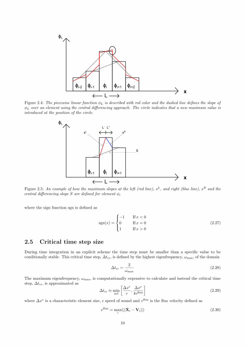
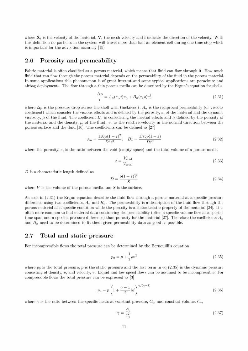
The Van Leer MUSCL Scheme is a scheme that is monotonic, conservative and second order accurate. Thisscheme is much slower than the Donor cell algorithm [19]. The principles of the Van Leer scheme is to include alinear variation of the field variable φ over an element. This is done by introducing a piecewise linear function,φL. The slope, S, of this piecewise linear function over an element in one dimension can be calculated by usingcentral differencing
Si =φi+1 − φi−1
L(2.24)
where i indicates the element. Using only the central differencing to calculate the slope over an element mayintroduce new minimum and maximum values as seen in Figure 2.4 and therefore another formulation is neededto ensure a monotonic scheme. In this new formulation the maximum allowed slope at the left and to the rightof an element are calculated. How these slopes are defined can be seen in Figure 2.5 together with the slopefrom the usage of central differencing. The maximum slope to the left, sL, and to the right, sR, are expressedas
sL =φi − φi−1
L−
sR =φi+1 − φi
L+
(2.25)
Now when the maximum slopes over an element are defined, the piecewise linear function with monotonicbehaviour are defined as
∂φL∂x
=1
2(sgn(sL) + sgn(sR)) min(|sL|, |sR|, |S|) (2.26)
9
x
ϕL
ϕi-2 ϕi-1 ϕi ϕi+1 ϕi+2
L
Figure 2.4: The piecewise linear function φL is described with red color and the dashed line defines the slope ofφL over an element using the central differencing approach. The circle indicates that a new maximum value isintroduced at the position of the circle.
x
ϕL
ϕi-1 ϕi ϕi+1
L
L-L+
sL
sR
S
Figure 2.5: An example of how the maximum slopes at the left (red line), sL, and right (blue line), sR and thecentral differencing slope S are defined for element φi
where the sign function sgn is defined as
sgn(x) =
−1 Ifx < 0
0 Ifx = 0
1 Ifx > 0
(2.27)
2.5 Critical time step size
During time integration in an explicit scheme the time step must be smaller than a specific value to beconditionally stable. This critical time step, ∆tcr, is defined by the highest eigenfrequency, ωmax, of the domain
∆tcr =2
ωmax(2.28)
The maximum eigenfrequency, ωmax, is computationally expensive to calculate and instead the critical timestep, ∆tcr, is approximated as
∆tcr ≈ minnel
[∆xe
c,
∆xe
4vflux
](2.29)
where ∆xe is a characteristic element size, c speed of sound and vflux is the flux velocity defined as
vflux = maxi
(||Xi −Vi||) (2.30)
10
where Xi is the velocity of the material, Vi the mesh velocity and i indicate the direction of the velocity. Withthis definition no particles in the system will travel more than half an element cell during one time step whichis important for the advection accuracy [19].
2.6 Porosity and permeability
Fabric material is often classified as a porous material, which means that fluid can flow through it. How muchfluid that can flow through the porous material depends on the permeability of the fluid in the porous material.In some applications this phenomenon is of great interest and some typical applications are parachute andairbag deployments. The flow through a thin porous media can be described by the Ergun’s equation for shells
∆p
t= An(ε, µ)vn +Bn(ε, ρ)v2
n (2.31)
where ∆p is the pressure drop across the shell with thickness t, An is the reciprocal permeability (or viscouscoefficient) which consider the viscous effects and is defined by the porosity, ε, of the material and the dynamicviscosity, µ of the fluid. The coefficient Bn is considering the inertial effects and is defined by the porosity ofthe material and the density, ρ, of the fluid. vn is the relative velocity in the normal direction between theporous surface and the fluid [16]. The coefficients can be defined as [27]
An =150µ(1− ε)2
D2ε3; Bn =
1.75ρ(1− ε)Dε3
(2.32)
where the porosity, ε, is the ratio between the void (empty space) and the total volume of a porous media
ε =Vvoid
Vtotal(2.33)
D is a characteristic length defined as
D =6(1− ε)V
S(2.34)
where V is the volume of the porous media and S is the surface.
As seen in (2.31) the Ergun equation describe the fluid flow through a porous material at a specific pressuredifference using two coefficients, An and Bn. The permeability is a description of the fluid flow through theporous material at a specific condition while the porosity is a characteristic property of the material [24]. It isoften more common to find material data considering the permeability (often a specific volume flow at a specifictime span and a specific pressure difference) than porosity for the material [27]. Therefore the coefficients Anand Bn need to be determined to fit these given permeability data as good as possible.
2.7 Total and static pressure
For incompressible flows the total pressure can be determined by the Bernouilli’s equation
p0 = p+1
2ρv2 (2.35)
where p0 is the total pressure, p is the static pressure and the last term in eq (2.35) is the dynamic pressureconsisting of density, ρ, and velocity, v. Liquid and low speed flows can be assumed to be incompressible. Forcompressible flows the total pressure can be expressed as [3]
po = p
(1 +
γ − 1
2M
)γ/(γ−1)
(2.36)
where γ is the ratio between the specific heats at constant pressure, Cp, and constant volume, Cv,
γ =CpCv
(2.37)
11
and M is the Mach number of the flowM =
v
a(2.38)
where a is the speed of sound in the fluid
a =
√γp
ρ(2.39)
For a gas, the speed of sound can be modified with the ideal gas law, p = ρRT
a =√γRT (2.40)
where R = Cp − Cv and T is the static temperature. It should be notated that for flows with low velocity,v → 0, the total pressure and the static pressure are almost equal
po ≈ p (2.41)
2.8 Artificial bulk viscosity
A shock wave gives rise to a discontinuous jump in pressure, density, particle velocity and energy. This kind ofdiscontinuous behaviour often results in numerical issues. To be able to solve this in a computer most wavepropagation codes use an artificial bulk viscosity [18]. This artificial bulk viscosity, q, is added to smear theshock so it changes rapidly but in a continuous way. In LS-DYNA this viscosity is defined as
q =
{ρl(C0lε
′2kk − C1aε
′kk) If ε′kk < 0
0 If ε′kk ≥ 0(2.42)
where C0 and C1 are dimensionless constants, a is the speed of sound, ρ is the density, l = 3√V is a characteristic
length based on the element volume V and ε′kk is the trace of the strain rate tensor defined in eq (2.6).
12
3 Simulation set-up
In this thesis the Finite Element based software LS-DYNA was used to create the model and to perform thecalculations. The simulations ran on a computer with 128 GB RAM and 16 cores. Several models have beenmade to evaluate how different parameters affect the acceleration of the bag. A case that was representinga clean bag at typical standard conditions was first made as a reference case. In the other cases only oneparameter was changed compared to the reference case. The study included:
• Different permeability of the bag
• Different weight of the dust cake
The simulations did not include dust particles in the flow. Only the dust that got stuck on the bag wereincluded as an extra weight on the bag. Also it was not possible to model turbulence in the MMALE methodand no account for boundary layer effects could be made [7]. All commandos used in the different cases couldbe seen in Appendix C.
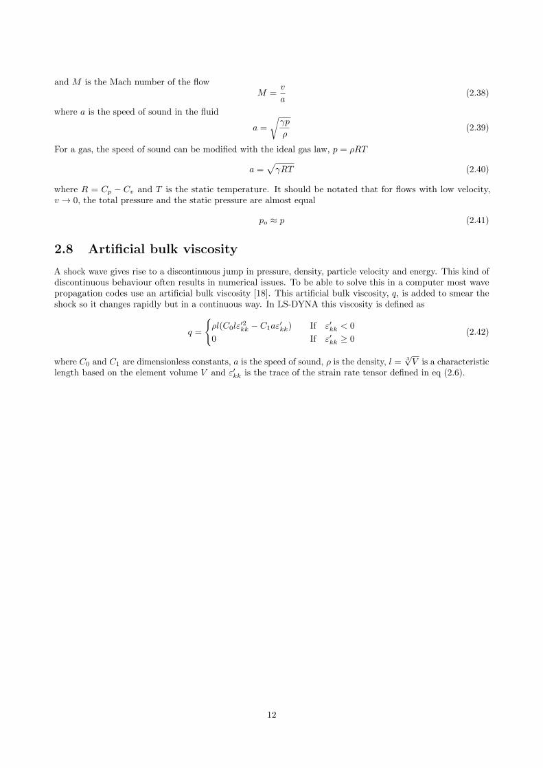
3.1 Geometry and model dimensions
All models contained the same parts with the same dimensions. All models included a nozzle, bag plate, bag,cage and three air domains. One air domain represents the air below the bag plate, one the air between thebag plate and the nozzle inlet and the last represents the air in a tank. The dimensions of the geometry couldbe seen in Figure 3.1 and 3.2 where D = 0.129 m, d = 0.04 m and L = 10 m. The cage consisted of eight rods
0.3 m
0.1 m
L+0.1 m
D
d
NozzleAir above
Bag
Air below
Bag plate
L
Air tank 0.1 m
Figure 3.1: Side view of the model geometry with cage parts excluded.
equally spaced on the inside of the bag and a plate, with slightly smaller dimensions than the bag, located nearthe bottom of the bag. The cage prevented the bag from crumpling when the air flowed through the filter. Thecage parts could be seen in Figure 3.3 together with the bag plate and the bag and by itself in Figure 3.4.The cage parts were located in such a way that it initially existed a gap of 1 mm between the bag and the cageparts. This was done to prevent initial penetration which could lead to non-physical accelerations in the bag.
13
0.3 m
0.3 m
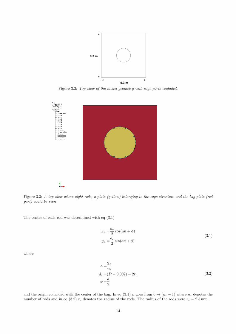
Figure 3.2: Top view of the model geometry with cage parts excluded.
Figure 3.3: A top view where eight rods, a plate (yellow) belonging to the cage structure and the bag plate (redpart) could be seen
The center of each rod was determined with eq (3.1)
xn =dc2
cos(an+ φ)
yn =dc2
sin(an+ φ)
(3.1)
where
a =2π
nrdc =(D − 0.002)− 2rc
φ =a
2
(3.2)
and the origin coincided with the center of the bag. In eq (3.1) n goes from 0→ (nr − 1) where nr denotes thenumber of rods and in eq (3.2) rc denotes the radius of the rods. The radius of the rods were rc = 2.5 mm.
14
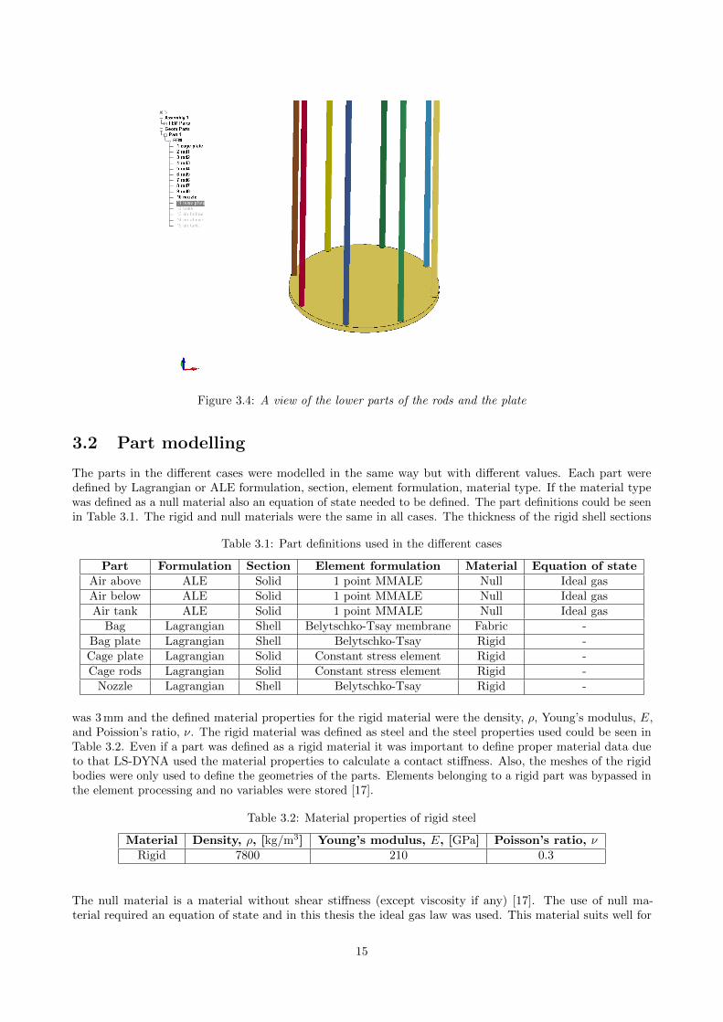
Figure 3.4: A view of the lower parts of the rods and the plate
3.2 Part modelling
The parts in the different cases were modelled in the same way but with different values. Each part weredefined by Lagrangian or ALE formulation, section, element formulation, material type. If the material typewas defined as a null material also an equation of state needed to be defined. The part definitions could be seenin Table 3.1. The rigid and null materials were the same in all cases. The thickness of the rigid shell sections
Table 3.1: Part definitions used in the different cases
Part Formulation Section Element formulation Material Equation of stateAir above ALE Solid 1 point MMALE Null Ideal gasAir below ALE Solid 1 point MMALE Null Ideal gasAir tank ALE Solid 1 point MMALE Null Ideal gas
Bag Lagrangian Shell Belytschko-Tsay membrane Fabric -Bag plate Lagrangian Shell Belytschko-Tsay Rigid -Cage plate Lagrangian Solid Constant stress element Rigid -Cage rods Lagrangian Solid Constant stress element Rigid -
Nozzle Lagrangian Shell Belytschko-Tsay Rigid -
was 3 mm and the defined material properties for the rigid material were the density, ρ, Young’s modulus, E,and Poission’s ratio, ν. The rigid material was defined as steel and the steel properties used could be seen inTable 3.2. Even if a part was defined as a rigid material it was important to define proper material data dueto that LS-DYNA used the material properties to calculate a contact stiffness. Also, the meshes of the rigidbodies were only used to define the geometries of the parts. Elements belonging to a rigid part was bypassed inthe element processing and no variables were stored [17].
Table 3.2: Material properties of rigid steel
Material Density, ρ, [kg/m3] Young’s modulus, E, [GPa] Poisson’s ratio, νRigid 7800 210 0.3
The null material is a material without shear stiffness (except viscosity if any) [17]. The use of null ma-terial required an equation of state and in this thesis the ideal gas law was used. This material suits well for
15
fluid-like materials. This material model was used to model the air and the properties defined were the density,ρ, and the dynamic viscosity, µ. These properties could be seen in Table 3.3. The properties of the equation ofstate for the standard condition (SC) could be seen in Table 3.4. The standard condition of the equation ofstate were used in all cases.
Table 3.3: Material properties for the null material
Material Density, ρ, [kg/m3] Dynamic viscosity, µ, [Pa · s]Null 1.2 1.85 · 10−5
Table 3.4: Equation of state properties at standard conditions (SC)
Equation of state Cv, [J/(kg ·K)] Cp, [J/(kg ·K)] Temperature, [K] Relative volume, ρo/ρIdeal gas (SC) 717 1004 295 1
The bag1 was modelled with a fabric material. This material was only supported for 3 or 4 nodes mem-brane elements [17] and this was the reason why this model ran as a 3D model instead of an axisymmetric 2Dmodel. The strain formulation used in the fabric model was the Green-Lagrange strain formulation due tothat relatively large deformation could occur. The properties defined for the fabric were the density, Young’smodulus, Poisson’s ratio and Ergun’s coefficients (to consider the permeability of the bag, see eq (2.32)). Thefabric was assumed to behave isotropic due to that deformations were mainly expected to occur in radialdirection due to influence of the cage bottom plate (no air could flow through the cage plate and thereforemost air would leave the bag in the radial direction). Both the density, ρ, and the Ergun’s coefficients An andBn needed to be calculated from known data. For the bag the area density, ρA, i.e mass per unit area wasknown and the following equation was used to calculate the density ρ of the bag
ρ =ρAt
(3.3)
where t was the thickness of the bag. Also the permeability was known for a specific pressure drop. It wasassumed that the pressure drop had a linear relation to the flow velocity2 and therefore the inertial coefficient,Bn, could be put to zero and only the viscous coefficient, An, was determined. Here an arbitrary value qdenotes the value of the permeability, vn
vn = qliters
dm2 ·minute(3.4)
The unit in eq (3.4) needed to be consistent and was rewritten to SI units and this resulted in
vn =q
600
m
s(3.5)
Equation (3.5) in eq (2.31) gave
An =∆p
t · vn= 600
∆p
t · q(3.6)
The properties of the bag differed between the cases and are instead presented under respective case ratherthan here.
3.3 Boundary conditions and loads
For a given problem the boundary conditions and loads must be defined for the parts in the model. Allinflow/outflow boundaries were set to be non-reflecting boundaries to avoid reflection when the air was flowingout of the domain. An alternative way to the non-reflecting boundaries could have been the use of an extralayer of AET (Ambient element type) on the boundaries of the domain [30]. The AET option could be foundin the element formulation and if it was used it defined the ambient conditions. The walls of the tank weremodelled with *ALE ESSENTIAL BOUNDARY where it was defined that no fluid could flow through thewalls.
1PPS/PPS 554 glaze CS31 bag2It is a quite linear correlation, as flow is very laminar inside the bag, according to the supplier at BWF Envirotec
16
Pressure loads on the ALE parts
The initial flow in the models resulted from a pressure difference, ∆p, between the air above and below the bagplate. Due to that the compressible solver was used it was not sufficient to just define the pressure differencebut also the absolute pressure was needed. The atmospheric pressure, patm, was set to be 100 kPa in all cases.The pressure below the bag plate, p1, was set to be the atmospheric pressure plus the pressure difference
p1 = patm + ∆p (3.7)
and the pressure above the bag plate, p2, was set equal to the atmospheric pressure
p2 = patm (3.8)
In reality a big tank was emptied and the flow was distributed over several nozzles and bags, but it was toocomputer demanding to consider all of them. Instead of simulating a full scale tank a pressure boundarycondition was used. The total pressure, p0(t), at the nozzle was known and was applied as a boundary condition
p0(t) = patm + p0,over(t) (3.9)
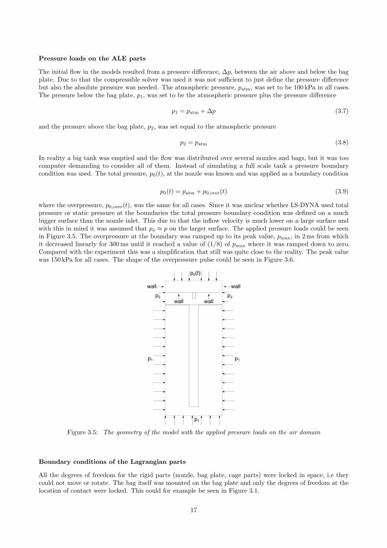
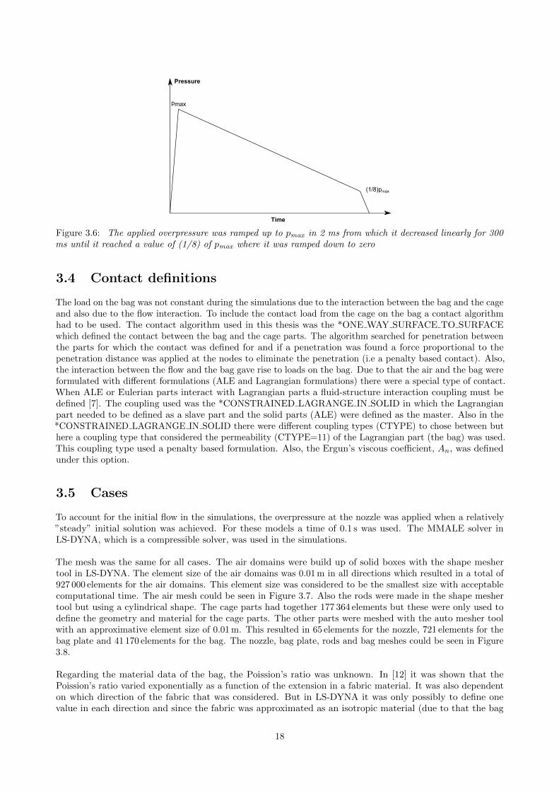
where the overpressure, p0,over(t), was the same for all cases. Since it was unclear whether LS-DYNA used totalpressure or static pressure at the boundaries the total pressure boundary condition was defined on a muchbigger surface than the nozzle inlet. This due to that the inflow velocity is much lower on a large surface andwith this in mind it was assumed that po ≈ p on the larger surface. The applied pressure loads could be seenin Figure 3.5. The overpressure at the boundary was ramped up to its peak value, pmax, in 2 ms from whichit decreased linearly for 300 ms until it reached a value of (1/8) of pmax where it was ramped down to zero.Compared with the experiment this was a simplification that still was quite close to the reality. The peak valuewas 150 kPa for all cases. The shape of the overpressure pulse could be seen in Figure 3.6.
p0(t)
p1 p1
p1
p2 p2
wall
wall wall
wall
Figure 3.5: The geometry of the model with the applied pressure loads on the air domain
Boundary conditions of the Lagrangian parts
All the degrees of freedom for the rigid parts (nozzle, bag plate, cage parts) were locked in space, i.e theycould not move or rotate. The bag itself was mounted on the bag plate and only the degrees of freedom at thelocation of contact were locked. This could for example be seen in Figure 3.1.
17
Pressure
Time
pmax
(1/8)pmax
Figure 3.6: The applied overpressure was ramped up to pmax in 2 ms from which it decreased linearly for 300ms until it reached a value of (1/8) of pmax where it was ramped down to zero
3.4 Contact definitions
The load on the bag was not constant during the simulations due to the interaction between the bag and the cageand also due to the flow interaction. To include the contact load from the cage on the bag a contact algorithmhad to be used. The contact algorithm used in this thesis was the *ONE WAY SURFACE TO SURFACEwhich defined the contact between the bag and the cage parts. The algorithm searched for penetration betweenthe parts for which the contact was defined for and if a penetration was found a force proportional to thepenetration distance was applied at the nodes to eliminate the penetration (i.e a penalty based contact). Also,the interaction between the flow and the bag gave rise to loads on the bag. Due to that the air and the bag wereformulated with different formulations (ALE and Lagrangian formulations) there were a special type of contact.When ALE or Eulerian parts interact with Lagrangian parts a fluid-structure interaction coupling must bedefined [7]. The coupling used was the *CONSTRAINED LAGRANGE IN SOLID in which the Lagrangianpart needed to be defined as a slave part and the solid parts (ALE) were defined as the master. Also in the*CONSTRAINED LAGRANGE IN SOLID there were different coupling types (CTYPE) to chose between buthere a coupling type that considered the permeability (CTYPE=11) of the Lagrangian part (the bag) was used.This coupling type used a penalty based formulation. Also, the Ergun’s viscous coefficient, An, was definedunder this option.
3.5 Cases
To account for the initial flow in the simulations, the overpressure at the nozzle was applied when a relatively”steady” initial solution was achieved. For these models a time of 0.1 s was used. The MMALE solver inLS-DYNA, which is a compressible solver, was used in the simulations.
The mesh was the same for all cases. The air domains were build up of solid boxes with the shape meshertool in LS-DYNA. The element size of the air domains was 0.01 m in all directions which resulted in a total of927 000 elements for the air domains. This element size was considered to be the smallest size with acceptablecomputational time. The air mesh could be seen in Figure 3.7. Also the rods were made in the shape meshertool but using a cylindrical shape. The cage parts had together 177 364 elements but these were only used todefine the geometry and material for the cage parts. The other parts were meshed with the auto mesher toolwith an approximative element size of 0.01 m. This resulted in 65 elements for the nozzle, 721 elements for thebag plate and 41 170 elements for the bag. The nozzle, bag plate, rods and bag meshes could be seen in Figure3.8.
Regarding the material data of the bag, the Poission’s ratio was unknown. In [12] it was shown that thePoission’s ratio varied exponentially as a function of the extension in a fabric material. It was also dependenton which direction of the fabric that was considered. But in LS-DYNA it was only possibly to define onevalue in each direction and since the fabric was approximated as an isotropic material (due to that the bag
18
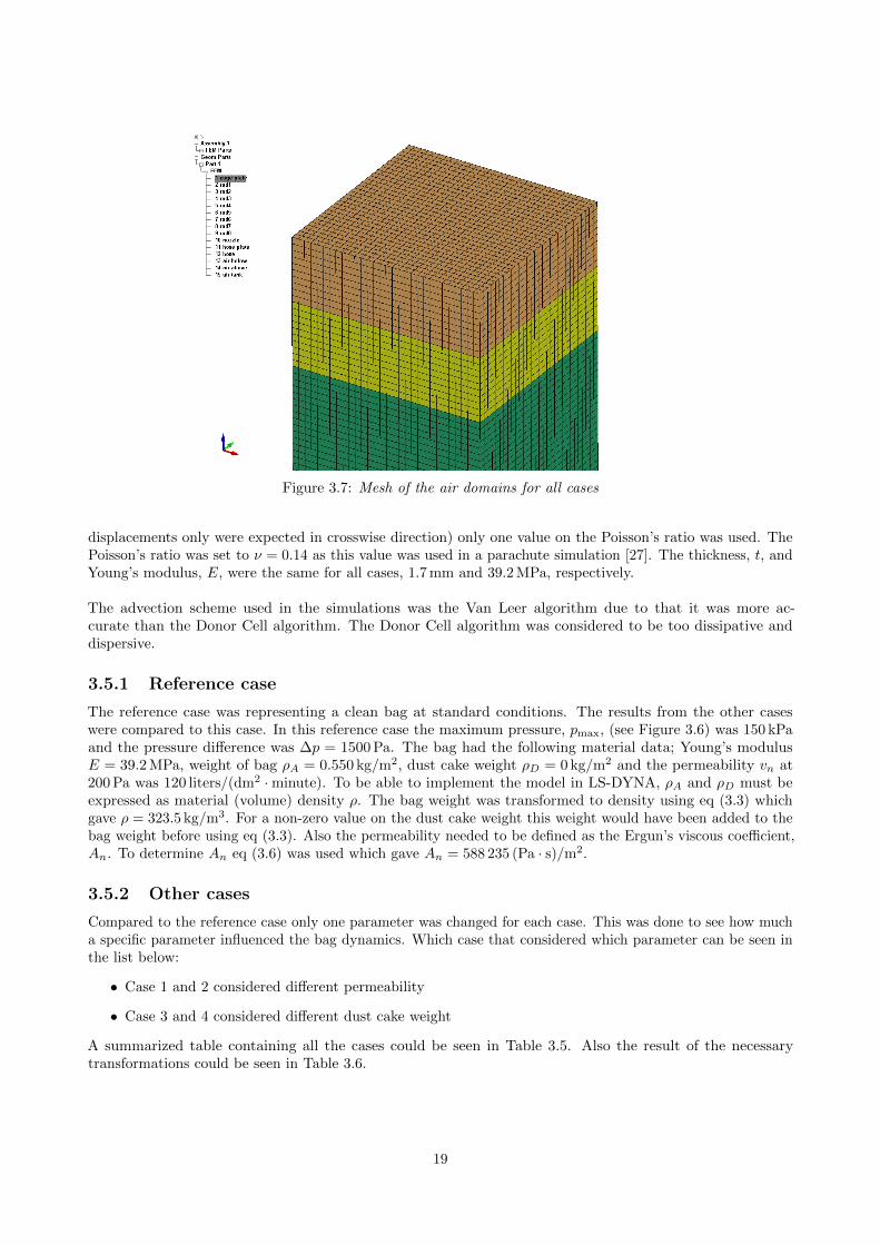
Figure 3.7: Mesh of the air domains for all cases
displacements only were expected in crosswise direction) only one value on the Poisson’s ratio was used. ThePoisson’s ratio was set to ν = 0.14 as this value was used in a parachute simulation [27]. The thickness, t, andYoung’s modulus, E, were the same for all cases, 1.7 mm and 39.2 MPa, respectively.
The advection scheme used in the simulations was the Van Leer algorithm due to that it was more ac-curate than the Donor Cell algorithm. The Donor Cell algorithm was considered to be too dissipative anddispersive.
3.5.1 Reference case
The reference case was representing a clean bag at standard conditions. The results from the other caseswere compared to this case. In this reference case the maximum pressure, pmax, (see Figure 3.6) was 150 kPaand the pressure difference was ∆p = 1500 Pa. The bag had the following material data; Young’s modulusE = 39.2 MPa, weight of bag ρA = 0.550 kg/m2, dust cake weight ρD = 0 kg/m2 and the permeability vn at200 Pa was 120 liters/(dm2 ·minute). To be able to implement the model in LS-DYNA, ρA and ρD must beexpressed as material (volume) density ρ. The bag weight was transformed to density using eq (3.3) whichgave ρ = 323.5 kg/m3. For a non-zero value on the dust cake weight this weight would have been added to thebag weight before using eq (3.3). Also the permeability needed to be defined as the Ergun’s viscous coefficient,An. To determine An eq (3.6) was used which gave An = 588 235 (Pa · s)/m2.
3.5.2 Other cases
Compared to the reference case only one parameter was changed for each case. This was done to see how mucha specific parameter influenced the bag dynamics. Which case that considered which parameter can be seen inthe list below:
• Case 1 and 2 considered different permeability
• Case 3 and 4 considered different dust cake weight
A summarized table containing all the cases could be seen in Table 3.5. Also the result of the necessarytransformations could be seen in Table 3.6.
19
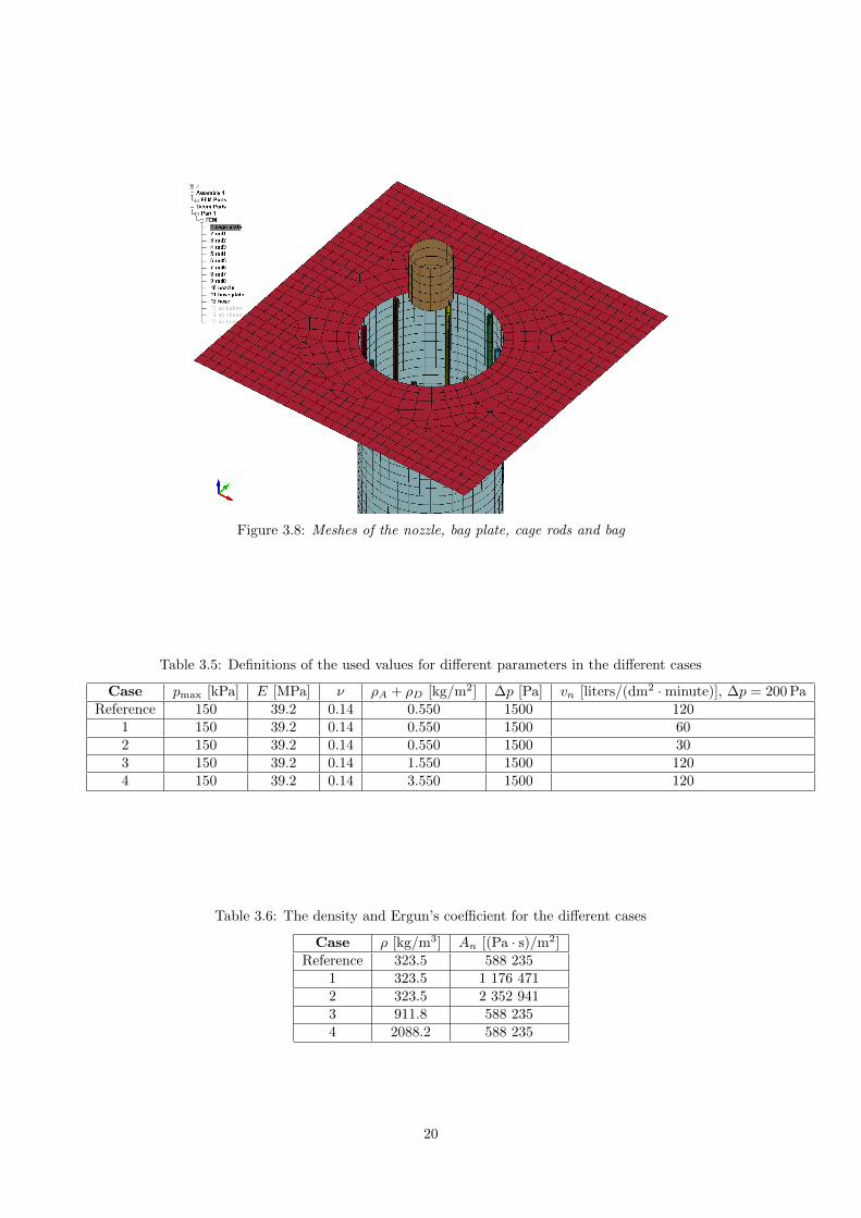
Figure 3.8: Meshes of the nozzle, bag plate, cage rods and bag
Table 3.5: Definitions of the used values for different parameters in the different cases
Case pmax [kPa] E [MPa] ν ρA + ρD [kg/m2] ∆p [Pa] vn [liters/(dm2 ·minute)], ∆p = 200 PaReference 150 39.2 0.14 0.550 1500 120
1 150 39.2 0.14 0.550 1500 602 150 39.2 0.14 0.550 1500 303 150 39.2 0.14 1.550 1500 1204 150 39.2 0.14 3.550 1500 120
Table 3.6: The density and Ergun’s coefficient for the different cases
Case ρ [kg/m3] An [(Pa · s)/m2]Reference 323.5 588 235
1 323.5 1 176 4712 323.5 2 352 9413 911.8 588 2354 2088.2 588 235
20
4 Result
In this chapter the results are presented. Some graphs look strange due to that there was some problem withviewing the results in the post-processor. There were some intervals where the results were missing which madeit hard to analyse the results. The reason for the problem was unknown, but probably it had something withthe hardware due to that LSTC did not have any problems when running the keyword-file on their computers.
4.1 Comparison with experiments
Some experimental results did exist and the data have been used to see how the ALE simulation of the bagpredicted this kind of physics. The known data were the total mass flow into a bag, pressure near the bagsurface and how long time it took for the pressure pulse to reach the cage plate located in the bottom of thebag. Most of the experimental results and the experiment set-up was confidential and could not be sheared inthis thesis. In this section the results from the simulation of a clean bag were compared with these knownexperimental data.
4.1.1 Mass of the inflowing air into a bag
To clean the bags a high pressure tank was emptied. The pressurized air was directed to the bags by severalnozzles. When the tank opens, the air flows from the tank to the nozzles until the pressure in the tank reachesatmospheric pressure i.e the mass representing the overpressure flows out of the tank. The mass of the airflowing out of the tank could be calculated as
mtank = ρtankVtank (4.1)
and together with the ideal gas law this could be expressed as
mtank =ptank
RTVtank (4.2)
where mtank is the mass, ptank is the tank overpressure, R is the gas constant for air, T is temperature andVtank is the tank volume. The volume that this mass occupies in atmospheric conditions can be calculated as
Vatm =m
ρatm(4.3)
where ρatm is the density in atmospheric conditions. This resulted in that 32.3 liters of air at atmosphericconditions was flowing into each bag. This value could be checked against the value of the mass flow inthe model. A function that calculates the mass flow through a surface in LS-DYNA was not found so anapproximation of the mass flow has been made instead. The mass flow rate can be expressed as
m = ρvA (4.4)
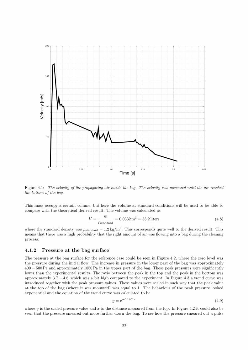
where m is the mass flow rate, ρ is the density of the air, v is the velocity of the air at the nozzle inlet and A isthe area of the nozzle. The velocity was assumed to behave linearly (same behaviour as the pressure at thenozzle) and to simplify the approximation a mean value of the velocity, v, was used. The velocity used was
v =vmax + vmin
2(4.5)
The velocities used in eq (4.5) was chosen to be vmax = 170 m/s and vmin = 0 m/s. The maximum velocitywas motivated by that this was the highest velocity of the inflowing air, as can be seen in Figure 4.1 and theminimum value will be zero when the tank pressure has reached atmospheric conditions. Also the densityvaried during the inflow and the mean value was put to be 1.25 kg/m3. Using eq (4.4) with nozzle diameter,d = 0.04 m, gives the average massflow rate through a nozzle as
¯m = 0.133 kg/s (4.6)
The total mass flow through a nozzle during the cleaning was (time t for the cleaning was approximately 300 ms)
m = ¯m · t = 0.0398 kg (4.7)
21
0
50
100
150
200
0 0.05 0.1 0.15 0.2 0.25
Vel
ocity
[m/s
]
Time [s]
Figure 4.1: The velocity of the propagating air inside the bag. The velocity was measured until the air reachedthe bottom of the bag.
This mass occupy a certain volume, but here the volume at standard conditions will be used to be able tocompare with the theoretical derived result. The volume was calculated as
V =m
ρstandard= 0.0332 m3 = 33.2 liters (4.8)
where the standard density was ρstandard = 1.2 kg/m3. This corresponds quite well to the derived result. Thismeans that there was a high probability that the right amount of air was flowing into a bag during the cleaningprocess.
4.1.2 Pressure at the bag surface
The pressure at the bag surface for the reference case could be seen in Figure 4.2, where the zero level wasthe pressure during the initial flow. The increase in pressure in the lower part of the bag was approximately400− 500 Pa and approximately 1850 Pa in the upper part of the bag. These peak pressures were significantlylower than the experimental results. The ratio between the peak in the top and the peak in the bottom wasapproximately 3.7− 4.6 which was a bit high compared to the experiment. In Figure 4.3 a trend curve wasintroduced together with the peak pressure values. These values were scaled in such way that the peak valueat the top of the bag (where it was mounted) was equal to 1. The behaviour of the peak pressure lookedexponential and the equation of the trend curve was calculated to be
y = e−0.1801x (4.9)
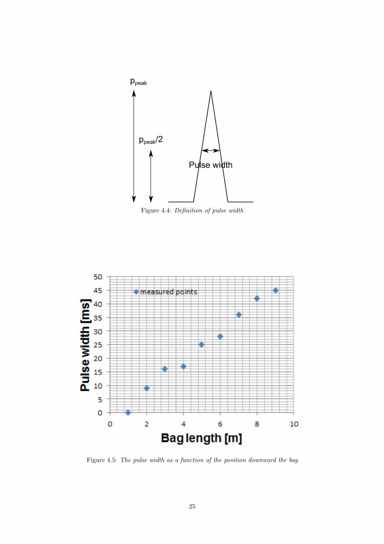
where y is the scaled pressure value and x is the distance measured from the top. In Figure 4.2 it could also beseen that the pressure smeared out more further down the bag. To see how the pressure smeared out a pulse
22
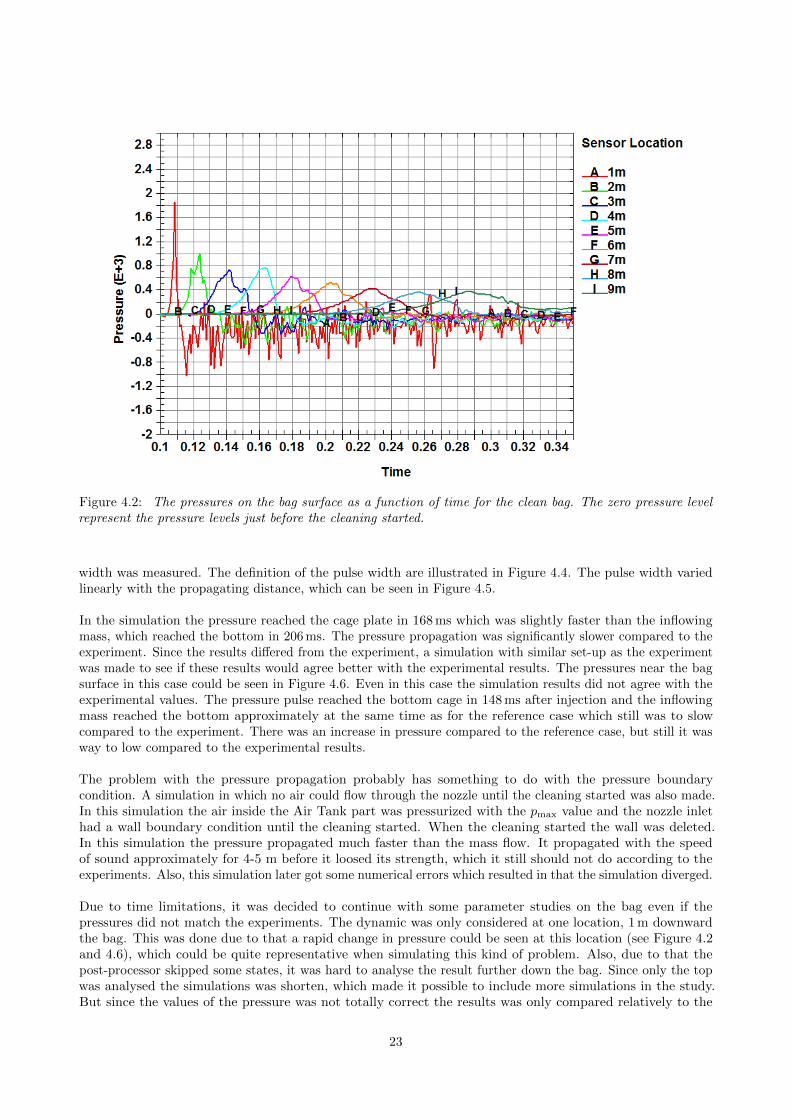
Figure 4.2: The pressures on the bag surface as a function of time for the clean bag. The zero pressure levelrepresent the pressure levels just before the cleaning started.
width was measured. The definition of the pulse width are illustrated in Figure 4.4. The pulse width variedlinearly with the propagating distance, which can be seen in Figure 4.5.
In the simulation the pressure reached the cage plate in 168 ms which was slightly faster than the inflowingmass, which reached the bottom in 206 ms. The pressure propagation was significantly slower compared to theexperiment. Since the results differed from the experiment, a simulation with similar set-up as the experimentwas made to see if these results would agree better with the experimental results. The pressures near the bagsurface in this case could be seen in Figure 4.6. Even in this case the simulation results did not agree with theexperimental values. The pressure pulse reached the bottom cage in 148 ms after injection and the inflowingmass reached the bottom approximately at the same time as for the reference case which still was to slowcompared to the experiment. There was an increase in pressure compared to the reference case, but still it wasway to low compared to the experimental results.
The problem with the pressure propagation probably has something to do with the pressure boundarycondition. A simulation in which no air could flow through the nozzle until the cleaning started was also made.In this simulation the air inside the Air Tank part was pressurized with the pmax value and the nozzle inlethad a wall boundary condition until the cleaning started. When the cleaning started the wall was deleted.In this simulation the pressure propagated much faster than the mass flow. It propagated with the speedof sound approximately for 4-5 m before it loosed its strength, which it still should not do according to theexperiments. Also, this simulation later got some numerical errors which resulted in that the simulation diverged.
Due to time limitations, it was decided to continue with some parameter studies on the bag even if thepressures did not match the experiments. The dynamic was only considered at one location, 1 m downwardthe bag. This was done due to that a rapid change in pressure could be seen at this location (see Figure 4.2and 4.6), which could be quite representative when simulating this kind of problem. Also, due to that thepost-processor skipped some states, it was hard to analyse the result further down the bag. Since only the topwas analysed the simulations was shorten, which made it possible to include more simulations in the study.But since the values of the pressure was not totally correct the results was only compared relatively to the
23
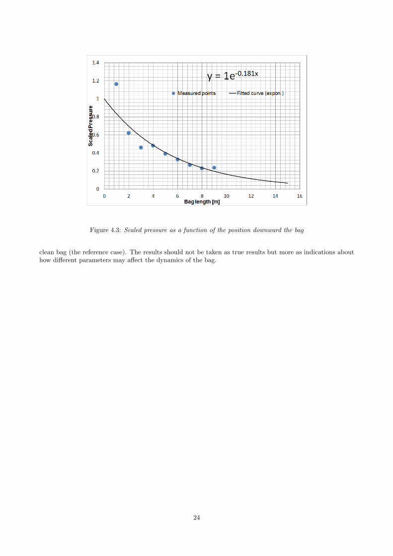
Figure 4.3: Scaled pressure as a function of the position downward the bag
clean bag (the reference case). The results should not be taken as true results but more as indications abouthow different parameters may affect the dynamics of the bag.
24
ppeak
ppeak/2
Pulse width
Figure 4.4: Definition of pulse width
Figure 4.5: The pulse width as a function of the position downward the bag
25
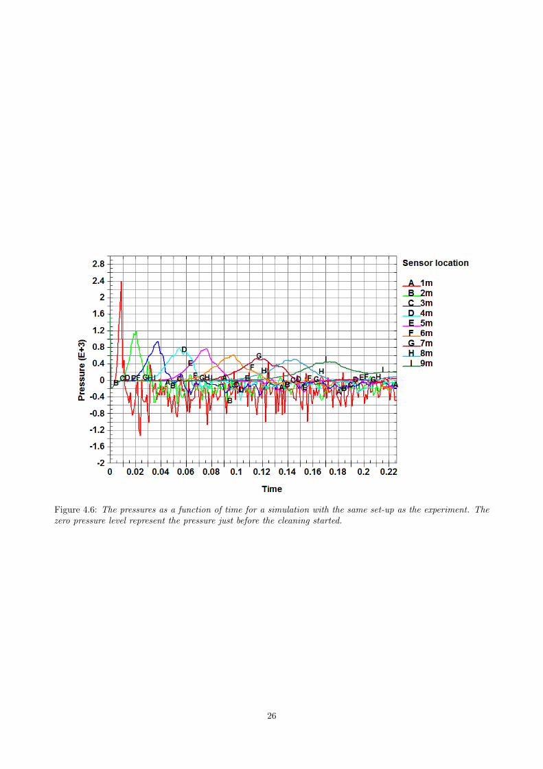
Figure 4.6: The pressures as a function of time for a simulation with the same set-up as the experiment. Thezero pressure level represent the pressure just before the cleaning started.
26
4.2 Reference case
The reference case representing a clean bag was used to compare the relative change between the differentcases. This was done to see how the cases differed when some specific parameter was changed. The main areaof interest was to see how the bag was affected during the cleaning. To get a better understanding of thedynamics of the bag, also the flow was analysed.
4.2.1 Flow characteristics
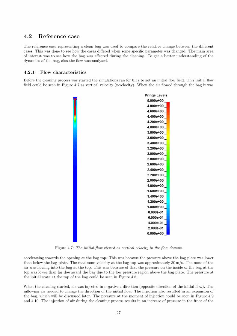
Before the cleaning process was started the simulations ran for 0.1 s to get an initial flow field. This initial flowfield could be seen in Figure 4.7 as vertical velocity (z-velocity). When the air flowed through the bag it was
Figure 4.7: The initial flow viewed as vertical velocity in the flow domain
accelerating towards the opening at the bag top. This was because the pressure above the bag plate was lowerthan below the bag plate. The maximum velocity at the bag top was approximately 30 m/s. The most of theair was flowing into the bag at the top. This was because of that the pressure on the inside of the bag at thetop was lower than far downward the bag due to the low pressure region above the bag plate. The pressure atthe initial state at the top of the bag could be seen in Figure 4.8.
When the cleaning started, air was injected in negative z-direction (opposite direction of the initial flow). Theinflowing air needed to change the direction of the initial flow. The injection also resulted in an expansion ofthe bag, which will be discussed later. The pressure at the moment of injection could be seen in Figure 4.9and 4.10. The injection of air during the cleaning process results in an increase of pressure in the front of the
27
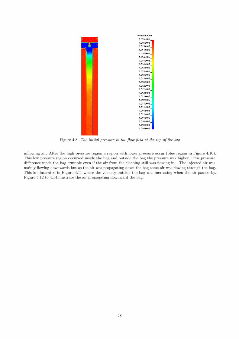
Figure 4.8: The initial pressure in the flow field at the top of the bag
inflowing air. After the high pressure region a region with lower pressure occur (blue region in Figure 4.10).This low pressure region occurred inside the bag and outside the bag the pressure was higher. This pressuredifference made the bag crumple even if the air from the cleaning still was flowing in. The injected air wasmainly flowing downwards but as the air was propagating down the bag some air was flowing through the bag.This is illustrated in Figure 4.11 where the velocity outside the bag was increasing when the air passed by.Figure 4.12 to 4.14 illustrate the air propagating downward the bag.
28
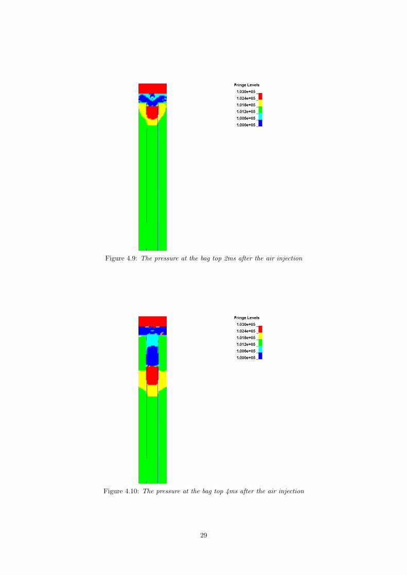
Figure 4.9: The pressure at the bag top 2ms after the air injection
Figure 4.10: The pressure at the bag top 4ms after the air injection
29
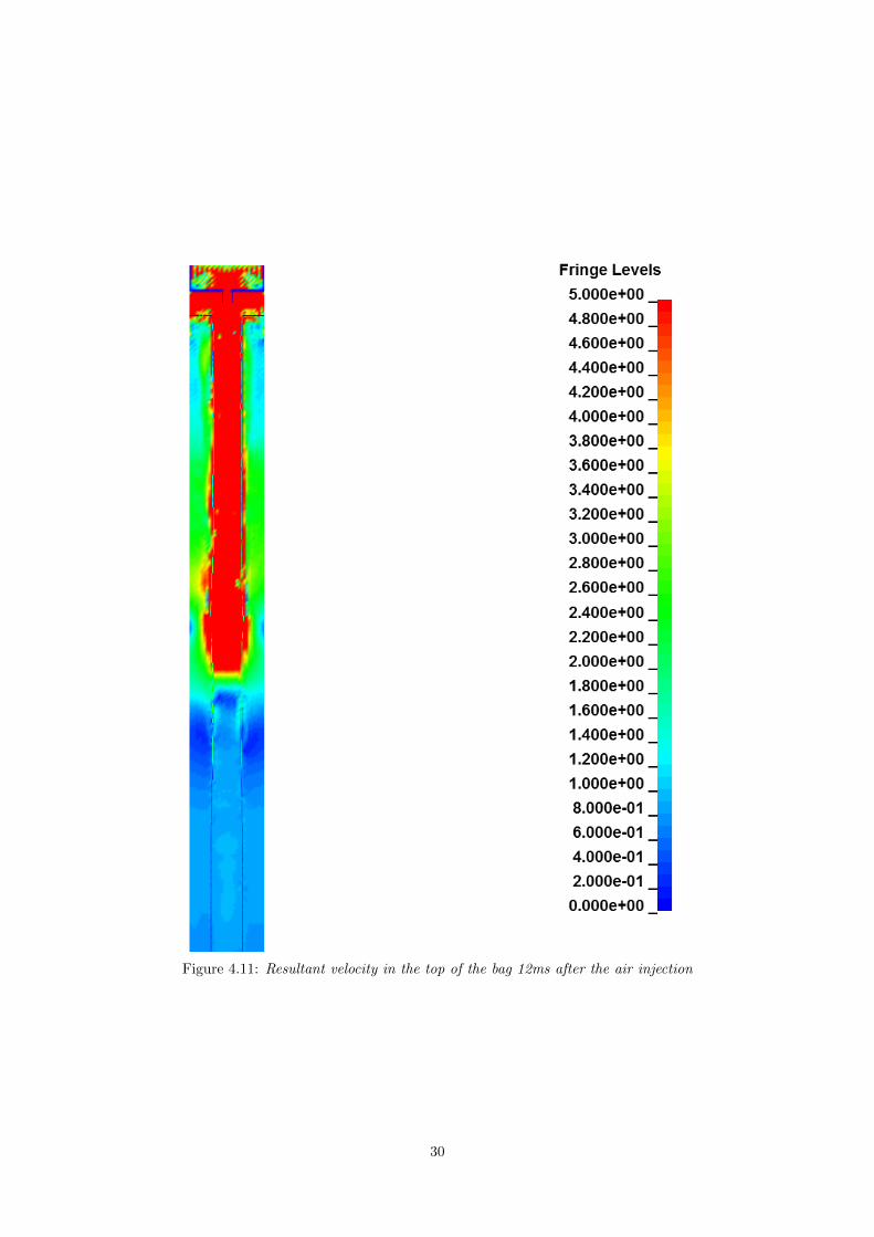
Figure 4.11: Resultant velocity in the top of the bag 12ms after the air injection
30
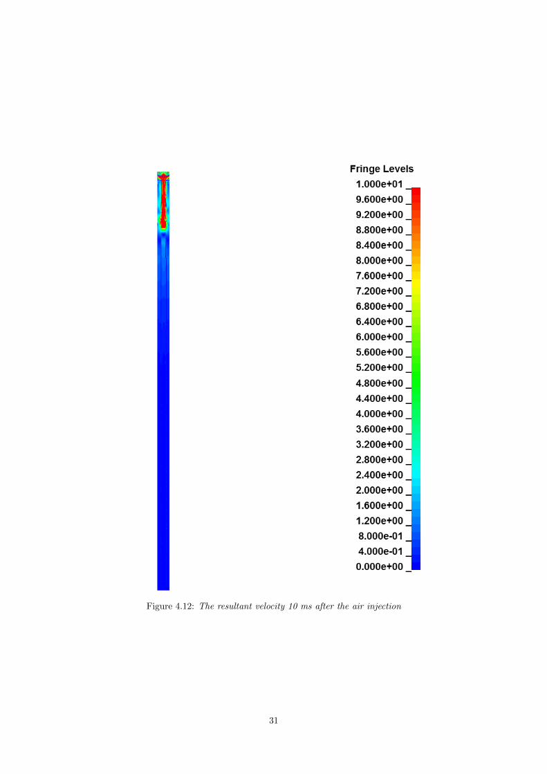
Figure 4.12: The resultant velocity 10 ms after the air injection
31
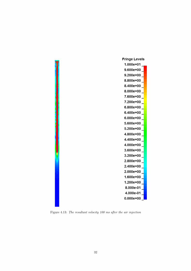
Figure 4.13: The resultant velocity 100 ms after the air injection
32
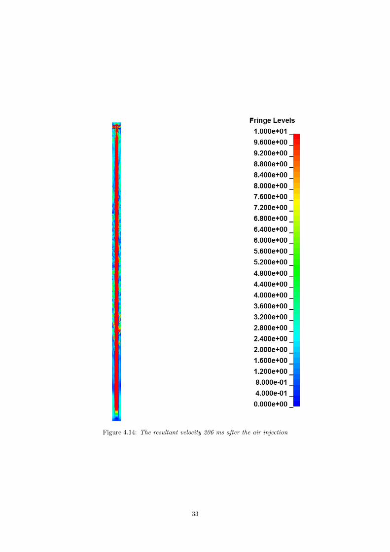
Figure 4.14: The resultant velocity 206 ms after the air injection
33
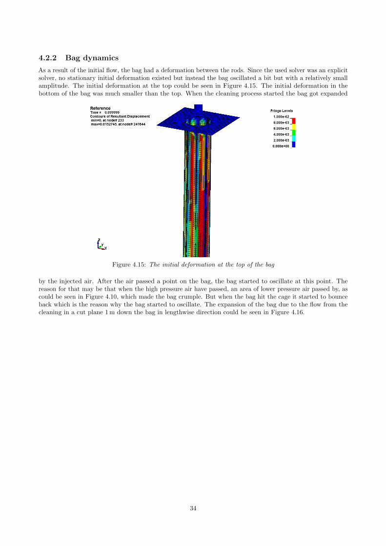
4.2.2 Bag dynamics
As a result of the initial flow, the bag had a deformation between the rods. Since the used solver was an explicitsolver, no stationary initial deformation existed but instead the bag oscillated a bit but with a relatively smallamplitude. The initial deformation at the top could be seen in Figure 4.15. The initial deformation in thebottom of the bag was much smaller than the top. When the cleaning process started the bag got expanded
Figure 4.15: The initial deformation at the top of the bag
by the injected air. After the air passed a point on the bag, the bag started to oscillate at this point. Thereason for that may be that when the high pressure air have passed, an area of lower pressure air passed by, ascould be seen in Figure 4.10, which made the bag crumple. But when the bag hit the cage it started to bounceback which is the reason why the bag started to oscillate. The expansion of the bag due to the flow from thecleaning in a cut plane 1 m down the bag in lengthwise direction could be seen in Figure 4.16.
34
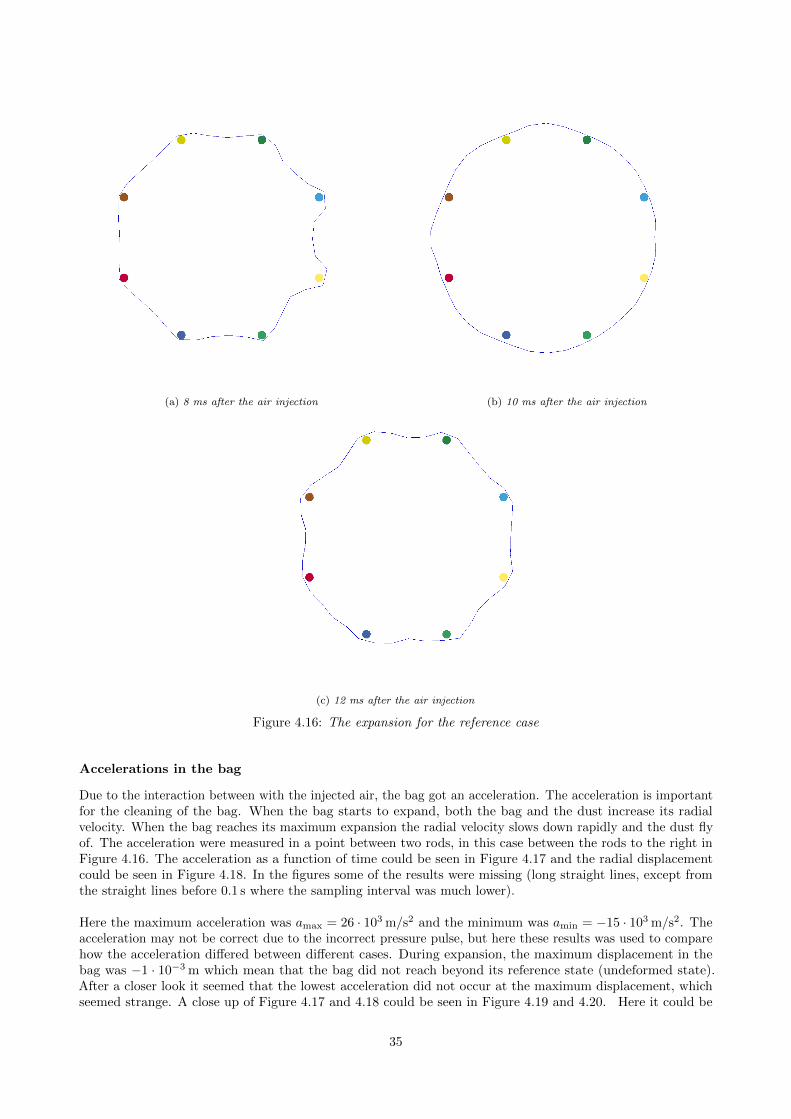
(a) 8 ms after the air injection (b) 10 ms after the air injection
(c) 12 ms after the air injection
Figure 4.16: The expansion for the reference case
Accelerations in the bag
Due to the interaction between with the injected air, the bag got an acceleration. The acceleration is importantfor the cleaning of the bag. When the bag starts to expand, both the bag and the dust increase its radialvelocity. When the bag reaches its maximum expansion the radial velocity slows down rapidly and the dust flyof. The acceleration were measured in a point between two rods, in this case between the rods to the right inFigure 4.16. The acceleration as a function of time could be seen in Figure 4.17 and the radial displacementcould be seen in Figure 4.18. In the figures some of the results were missing (long straight lines, except fromthe straight lines before 0.1 s where the sampling interval was much lower).
Here the maximum acceleration was amax = 26 · 103 m/s2 and the minimum was amin = −15 · 103 m/s2. Theacceleration may not be correct due to the incorrect pressure pulse, but here these results was used to comparehow the acceleration differed between different cases. During expansion, the maximum displacement in thebag was −1 · 10−3 m which mean that the bag did not reach beyond its reference state (undeformed state).After a closer look it seemed that the lowest acceleration did not occur at the maximum displacement, whichseemed strange. A close up of Figure 4.17 and 4.18 could be seen in Figure 4.19 and 4.20. Here it could be
35
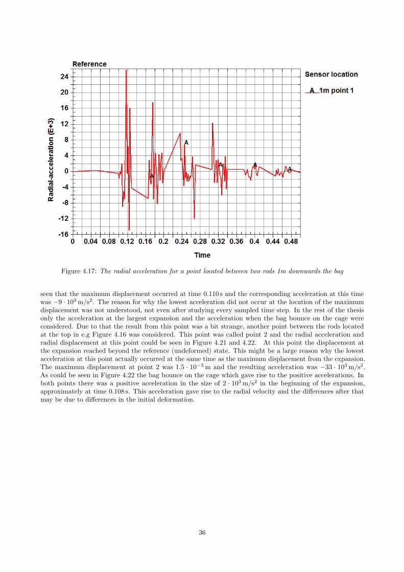
Figure 4.17: The radial acceleration for a point located between two rods 1m downwards the bag
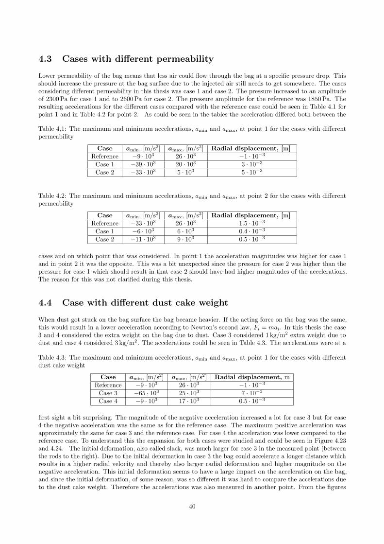
seen that the maximum displacement occurred at time 0.110 s and the corresponding acceleration at this timewas −9 · 103 m/s2. The reason for why the lowest acceleration did not occur at the location of the maximumdisplacement was not understood, not even after studying every sampled time step. In the rest of the thesisonly the acceleration at the largest expansion and the acceleration when the bag bounce on the cage wereconsidered. Due to that the result from this point was a bit strange, another point between the rods locatedat the top in e.g Figure 4.16 was considered. This point was called point 2 and the radial acceleration andradial displacement at this point could be seen in Figure 4.21 and 4.22. At this point the displacement atthe expansion reached beyond the reference (undeformed) state. This might be a large reason why the lowestacceleration at this point actually occurred at the same time as the maximum displacement from the expansion.The maximum displacement at point 2 was 1.5 · 10−3 m and the resulting acceleration was −33 · 103 m/s2.As could be seen in Figure 4.22 the bag bounce on the cage which gave rise to the positive accelerations. Inboth points there was a positive acceleration in the size of 2 · 103 m/s2 in the beginning of the expansion,approximately at time 0.108 s. This acceleration gave rise to the radial velocity and the differences after thatmay be due to differences in the initial deformation.
36
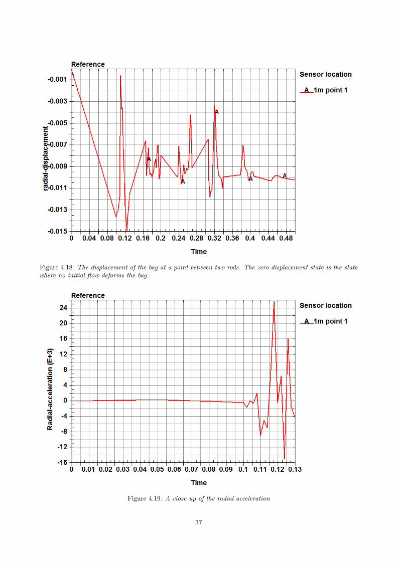
Figure 4.18: The displacement of the bag at a point between two rods. The zero displacement state is the statewhere no initial flow deforms the bag.
Figure 4.19: A close up of the radial acceleration
37
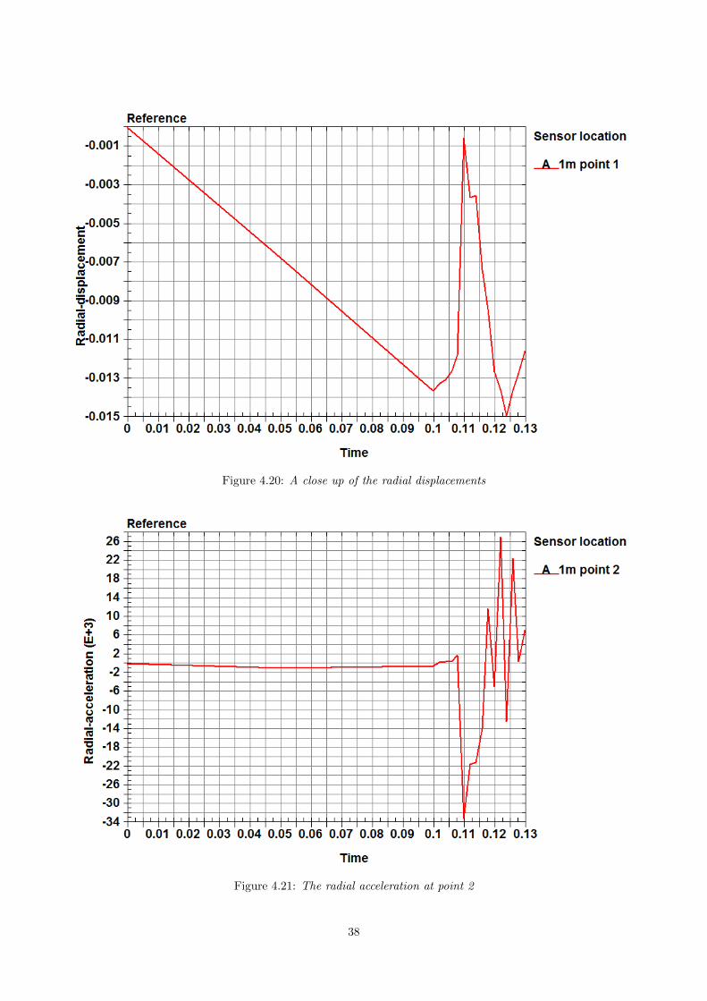
Figure 4.20: A close up of the radial displacements
Figure 4.21: The radial acceleration at point 2
38
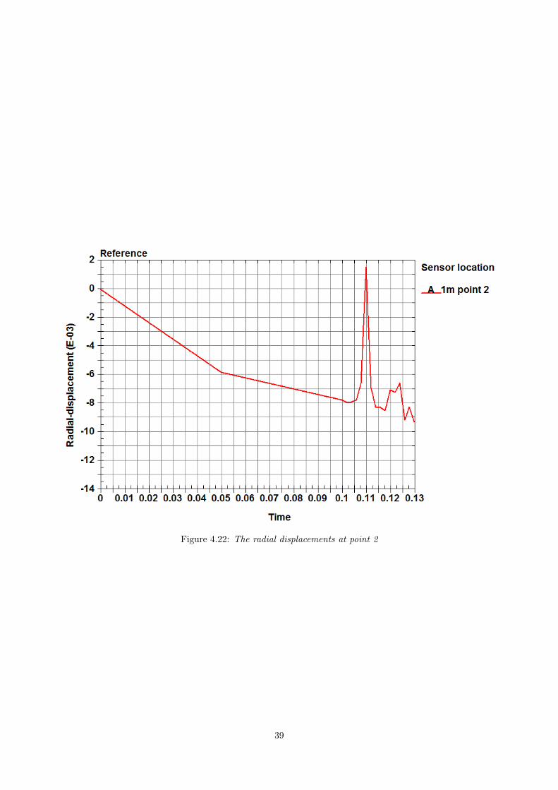
Figure 4.22: The radial displacements at point 2
39
4.3 Cases with different permeability
Lower permeability of the bag means that less air could flow through the bag at a specific pressure drop. Thisshould increase the pressure at the bag surface due to the injected air still needs to get somewhere. The casesconsidering different permeability in this thesis was case 1 and case 2. The pressure increased to an amplitudeof 2300 Pa for case 1 and to 2600 Pa for case 2. The pressure amplitude for the reference was 1850 Pa. Theresulting accelerations for the different cases compared with the reference case could be seen in Table 4.1 forpoint 1 and in Table 4.2 for point 2. As could be seen in the tables the acceleration differed both between the
Table 4.1: The maximum and minimum accelerations, amin and amax, at point 1 for the cases with differentpermeability
Case amin, [m/s2] amax, [m/s2] Radial displacement, [m]Reference −9 · 103 26 · 103 −1 · 10−3
Case 1 −39 · 103 20 · 103 3 · 10−3
Case 2 −33 · 103 5 · 103 5 · 10−3
Table 4.2: The maximum and minimum accelerations, amin and amax, at point 2 for the cases with differentpermeability
Case amin, [m/s2] amax, [m/s2] Radial displacement, [m]Reference −33 · 103 26 · 103 1.5 · 10−3
Case 1 −6 · 103 6 · 103 0.4 · 10−3
Case 2 −11 · 103 9 · 103 0.5 · 10−3
cases and on which point that was considered. In point 1 the acceleration magnitudes was higher for case 1and in point 2 it was the opposite. This was a bit unexpected since the pressure for case 2 was higher than thepressure for case 1 which should result in that case 2 should have had higher magnitudes of the accelerations.The reason for this was not clarified during this thesis.
4.4 Case with different dust cake weight
When dust got stuck on the bag surface the bag became heavier. If the acting force on the bag was the same,this would result in a lower acceleration according to Newton’s second law, Fi = mai. In this thesis the case3 and 4 considered the extra weight on the bag due to dust. Case 3 considered 1 kg/m2 extra weight due todust and case 4 considered 3 kg/m2. The accelerations could be seen in Table 4.3. The accelerations were at a
Table 4.3: The maximum and minimum accelerations, amin and amax, at point 1 for the cases with differentdust cake weight
Case amin, [m/s2] amax, [m/s2] Radial displacement, mReference −9 · 103 26 · 103 −1 · 10−3
Case 3 −65 · 103 25 · 103 7 · 10−3
Case 4 −9 · 103 17 · 103 0.5 · 10−3
first sight a bit surprising. The magnitude of the negative acceleration increased a lot for case 3 but for case4 the negative acceleration was the same as for the reference case. The maximum positive acceleration wasapproximately the same for case 3 and the reference case. For case 4 the acceleration was lower compared to thereference case. To understand this the expansion for both cases were studied and could be seen in Figure 4.23and 4.24. The initial deformation, also called slack, was much larger for case 3 in the measured point (betweenthe rods to the right). Due to the initial deformation in case 3 the bag could accelerate a longer distance whichresults in a higher radial velocity and thereby also larger radial deformation and higher magnitude on thenegative acceleration. This initial deformation seems to have a large impact on the acceleration on the bag,and since the initial deformation, of some reason, was so different it was hard to compare the accelerations dueto the dust cake weight. Therefore the accelerations was also measured in another point. From the figures
40
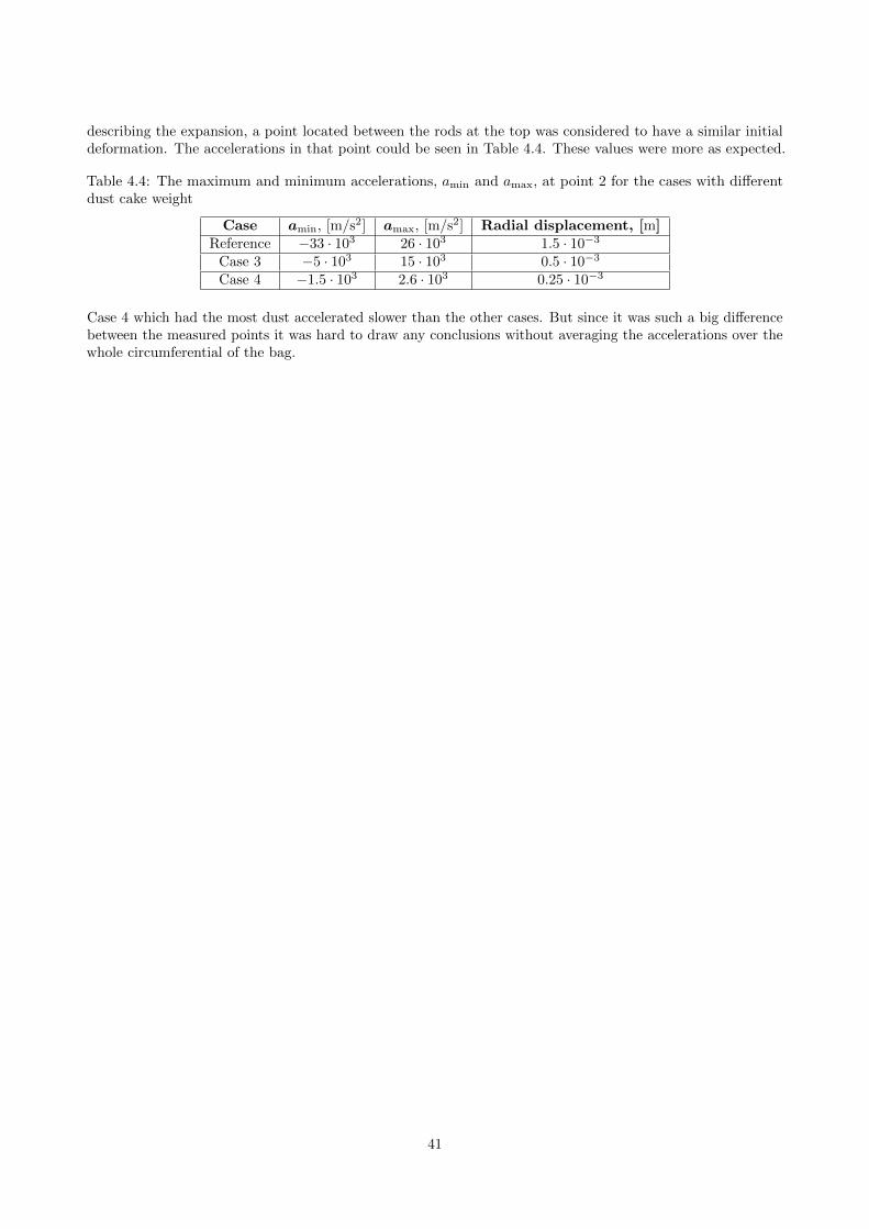
describing the expansion, a point located between the rods at the top was considered to have a similar initialdeformation. The accelerations in that point could be seen in Table 4.4. These values were more as expected.
Table 4.4: The maximum and minimum accelerations, amin and amax, at point 2 for the cases with differentdust cake weight
Case amin, [m/s2] amax, [m/s2] Radial displacement, [m]Reference −33 · 103 26 · 103 1.5 · 10−3
Case 3 −5 · 103 15 · 103 0.5 · 10−3
Case 4 −1.5 · 103 2.6 · 103 0.25 · 10−3
Case 4 which had the most dust accelerated slower than the other cases. But since it was such a big differencebetween the measured points it was hard to draw any conclusions without averaging the accelerations over thewhole circumferential of the bag.
41
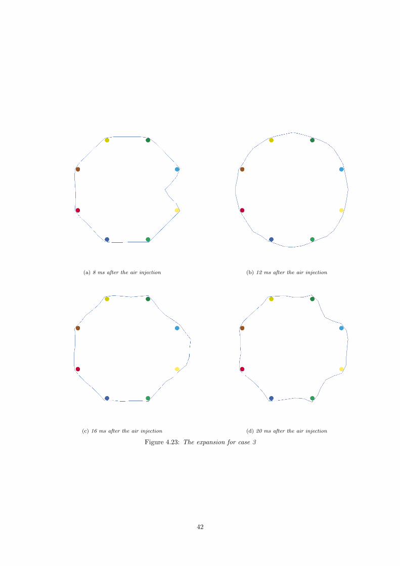
(a) 8 ms after the air injection (b) 12 ms after the air injection
(c) 16 ms after the air injection (d) 20 ms after the air injection
Figure 4.23: The expansion for case 3
42
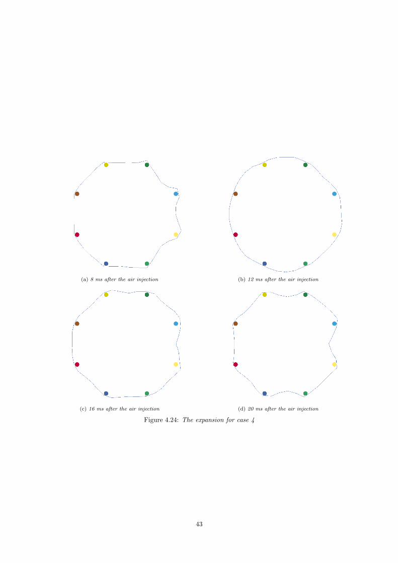
(a) 8 ms after the air injection (b) 12 ms after the air injection
(c) 16 ms after the air injection (d) 20 ms after the air injection
Figure 4.24: The expansion for case 4
43
5 Discussion
The simulations made in this thesis failed to predict the pressure pulse during the injection. According toexperiments, the pressure pulse should propagate significantly faster and with a higher magnitude than predictedfrom the simulations. The reason for this have probably something to do with the pressure boundary conditionabove the nozzle (the surface where the air injection occur). This boundary condition, describing the totalpressure, have been tested in several ways. At first, the boundary condition was put at the nozzle inlet. Butsince the pressure pulse did not propagate correctly a new boundary condition was set on a larger surface. Thiswas done because it was unsure how LS-DYNA defined the pressure at a segment, i.e if it was static or totalpressure that was defined. The approach of defining the total pressure on a larger surface was made becauseof that the total pressure approximates the static pressure if the velocity is low. If the pressure boundarycondition was put on a larger surface, the velocity at the boundary would be lower and therefore the effectof the dynamic pressure would decrease. Still, this was not enough to solve the problem with the pressurepropagation. The next try was to pre-pressurize the air above the nozzle and prevent the air from flowingthrough the nozzle inlet until the cleaning process started. This was done with a wall boundary condition atthe nozzle inlet and was suddenly deleted when the cleaning process started. Here the pressure propagatedmuch faster. It actually propagated with the speed of sound, but unfortunately only for while and it also gotsome numerical issues and gave non-physical velocities through the bag. But from this simulation, it was shownthat just the pressure boundary condition was not sufficient to trigger the pressure pulse propagation correctly.Due to time limitation, it was decided to continue with some parameter studies. But if there was more time, itwould be a top priority to find a new way to model the injection. A way could be to model the full scale tankbut today that would be too computational demanding.
The acceleration in the bag was expected to increase with lower permeability due to that the pressureshould increase if less air was flowing through the bag surface (more air remains inside the bag). If dust gotstuck on the bag surface it was expected that the bag would react slower on the changes in the flow field due tohigher inertia and the acceleration magnitudes would decrease with the weight of the dust cake. But as couldbe seen in the result chapter, this was not the case. The trends were hard to predict and the expectations wereonly fulfilled at point 2 for the cases with different dust cake weight. The reason for the unexpected results wasprobably the uneven initial deformation (also called slack). The slack was much higher in one locations (point 1for all cases). In some cases the slack resulted in that the expansion did not reach the undeformed state, but incase 3 this initial slack was much larger than the other cases and this resulted in that the bag could accelerate fora longer distance. This resulted in that the bag expanded a lot. Since it seems that the initial slack affects theaccelerations a lot in the simulations, it could not be seen in the simulations how the studied parameters affectedthe bag. Since the simulations were transient, the initial deformation changed with time and therefore theaccelerations may have looked different if the injection should have started in a different time. Why there was anuneven slack in the simulations was not understood. It was expected to be approximately the same slack betweenall the rods, but this was not the case in the simulations. In reality, the number of rods are higher and the initialslack should be smaller than in the simulations. Also, since the accelerations differed a lot in different pointsin the same case, some kind of standard should be implemented about how the accelerations should be measured.
The initial deformation were much larger at the top compared to the bottom of the bag. In the simula-tions this was because the pressure difference between the inside and the outside of the bag was much largerat the top than the bottom due to the lower pressure above the bag plate. This resulted in that the most ofthe air flowed through the bag at the top and almost nothing in the bottom. This may not be the case inreality and the problem was probably because two pressure boundary conditions were used (i.e the pressuregradient, ∂p/∂xi, which drives the flow was larger at the top than the bottom). Maybe a velocity boundarycondition at the boundaries at the air part below the bag plate could have been a better choice. This velocitycould be estimated if the amount of air flowing into the fabric filter was known. Also the initial flow was onlyrunning for 0.1 s. Even if it seemed to be steady at a first sight, maybe a longer initial solution could affect thedeformations in the lower parts of the bag. But running the initial solution for a longer time is expensive. Dueto that LS-DYNA used an explicit solver, the time step needed to be small enough to be conditionally stable.In the simulations in this thesis the stable time step was between 1− 5 · 10−6 s and this resulted in many timesteps. The simulation of the reference case, which was simulated for 0.5 s, took 5-6 days on 16 cores. The othersimulations were shorter but still took approximately 2 days on 16 cores. Also [7] states that the compressibleALE solver in LS-DYNA was developed for short duration problems with high pressure and velocity gradients
44
and therefore does not suit well for flows with low pressure gradients.
5.1 Future work
This thesis was a first step of modelling the dynamics of a bag during cleaning. To be able to use this kind ofsimulations to improve the cleaning process, the model needs to be modified. A list of things that needs to bedone follows:
• The pressure pulse and injection of air needs to be modelled in such a way that the pressure propagatesfaster and with the right pressure magnitude. The amount of injected air should be approximately thesame as in this thesis.
• The initial deformation may need to be distributed in a more even way
• The dynamics of the bag should be investigated in the bottom of the bag to see if the lower parts of thebag get cleaned
• Also simulations of longer bags could be interesting, because longer bags could filter more air
• Fabric material often have anisotropic or orthotropic material behaviours and this could be included in afuture project
• The parameter studies could include more simulations on every case and also include other parameterslike different Young’s modulus, different size of the pressure pulse from the cleaning, different initial flow,different distribution of the dust on the bag etc
45
6 Conclusions
The aim of this thesis was to evaluate the dynamics of a bag when a pressure pulse was injected inside adeformable porous fabric bag. The simulations did not agree to experimental values but still it is too early toreject the modelling approach. If the injected air is modelled with another boundary condition it might bepossible to study the dynamics of the bag. This thesis shows that it might be possible to model the cleaning ofthe bag. The model included the fluid structure interaction between flowing air and a porous fabric. Also acontact between the bag and the cage was included to prevent the bag from to large deformation (crumpling).All this was included in the Arbitrary Lagrangian-Eulerian method. A great advantage of using the ALEmethod is the fact that it is only one code, which means that it does not have to communicate with otherprograms.
The dynamics of the bag showed different results in different points and a need of a standard of how theseresult should be measured needs to be defined if the results should make any sense. Also, since the solver wasan explicit solver there did not exist a steady initial solution. Therefore the initial solution differed at differenttimes and with different cases. The uneven slack in the simulations affected the bag in a way that was notunderstood at the time of this thesis. To be able to analyse the dynamics of the bag, the initial slack should becontrolled somehow so it does not affect the solution to much.
Since the model predicted the pressure pulse was not accurate in all respects, also the accelerations were notaccurate. But with improvement of the boundary condition, the modelling approach may be sufficient.
46
References
[1] ALSTOM. Air Quality Control Systems. Pure Air, Clean Solutions. Online; accessed 11-February-2014.url: http://www.alstom.com/Global/Power/Resources/Documents/Brochures/air- quality-control-systems.pdf.
[2] ALSTOM. NID Flue Gas Desulphurization. Online; accessed 11-February-2014. url: http://www.alstom.com/Global/Power/Resources/Documents/Brochures/nid-flue-gas-desulphurisation.pdf.
[3] J. D. Anderson. Modern Compressible Flow. with historical perspective. 3rd ed. McGraw-Hill, 2004. isbn:007-124136-1.
[4] N. Aquelet. ALE Adaptive Mesh Refinement in LS-DYNA. 12th International LS-DYNA Users Conference(2012).
[5] A. Bostrom. Rigid Body Dynamics. Oct. 2013.[6] L. Davidsson. Fluid mechanics, turbulent flow and turbulence modeling. Sept. 2012.[7] J. Day. Guidelines for ALE modelling in LS-DYNA. Oct. 2010.[8] A. Derviux et al. Total energy conservation in ALE schemes for compressible flows. European Journal of
Computational Mechanics (2010).[9] J Donea et al. “Arbitrary Lagrangian-Eulerian Methods”. Encyclopedia of Computational Mechanics.
Fundamentals. Vol. 1. John Wiley & Sons Ltd, 2004. isbn: 0-470-84699-2.[10] M. Ekh. TME075 Mechanics of solids - linear elasticity. Sept. 2012.[11] Environmental Protection Agancy - United States. Human Health and Environmental Effects of Emissions
from Power Generation. Online; accessed 11-February-2014. url: http://www.epa.gov/captrade/documents/power.pdf.
[12] N. Erzaz Shahabi, S. Saharkhiz, and S Mohmammad Hosseini Varkiyani. Effect of Fabric Structure andWeft Density on the Poission’s Rato of Worsted Fabric. Journal of Engineering Fibers and Fabrics (2013).
[13] M. Forsblom. “Supersonic Artillery Projectile Fin Deployment Simulation Methodology”. MA thesis.Lulea University of Technology, June 2013.
[14] Franhofer Institute for High-Speed Dynamics, Ernst-Mach-Institute. Characterization and Modeling ofFabric Materials. Online; accessed 21-April-2014. url: http://www.en.emi.fraunhofer.de/business-segments/transport/characterization-and-modeling-of-fabric-materials/.
[15] A. Haufe, K. Weimar, and U. Gohner. Advanced Airbagsimulation using Fluid-Structure-Interaction andthe Eulerian Method in LS-DYNA. 2004.
[16] Livermore Software Technology Corporation. LS DYNA - Keyword User’s Manual. Volume 1. 2014.[17] Livermore Software Technology Corporation. LS DYNA - Keyword User’s Manual. Volume 2. 2014.[18] Livermore Software Technology Corporation. LS-DYNA - Theory Manual. 2014.[19] L. Olovsson. Training class in ALE and fluid-structure interaction. 2006.[20] N. Ottosen and H. Petersson. Introduction to the Finite Element Method. Pearson, 1992. isbn: 978-0-13-
473877-2.[21] SIMULIA. Abaqus Analysis User’s Manual. Version 6.12.[22] SIMULIA. Simulation of Airbag Deployment Using Coupled Eulerian-Lagrangian Method in Abaqus/Explicit.
June 2011.[23] B. Sundstrom, ed. Handbok och formelsamling i Hallfasthetslara. Instutionen for hallfasthetslara KTH,
1999.[24] B. Tutt et al. Finite Mass Simulation Techniques in LS-DYNA. 21st AIAA Aerodynamic Decelerator
Systems Technology Conference and Seminar (2011).[25] B. Tutt. The Application of a New Material Porosity Algorithm for Parachute Analysis. 9th International
LS-DYNA Users Conference (2006).[26] B. Tutt et al. Development of Parachute Simulation Techniques in LS-DYNA. 11th International LS-DYNA
Users Conference (2010).[27] J. Wang et al. Porous Euler-Lagrange Coupling: Application to Parachute Dynamics. 9th International
LS-DYNA Users Conference (2006).[28] Wikipedia. Cauchy Stress Tensor — Wikipedia, The Free Encyclopedia. [Online; accessed 6-April-2014].
2013. url: http://en.wikipedia.org/wiki/Cauchy_stress_tensor.[29] G. Xing-long et al. Fluid-Structure Interaction Simulation of Parachute in Low Speed Airdrop. Proceedings
of the World Congress on Engineering 3 (July 2013).
47
[30] R. Zong. “Finite Element Analysis of ship-ice collision using LS-DYNA”. MA thesis. Memorial Universityof Newfoundland, July 2012.
48
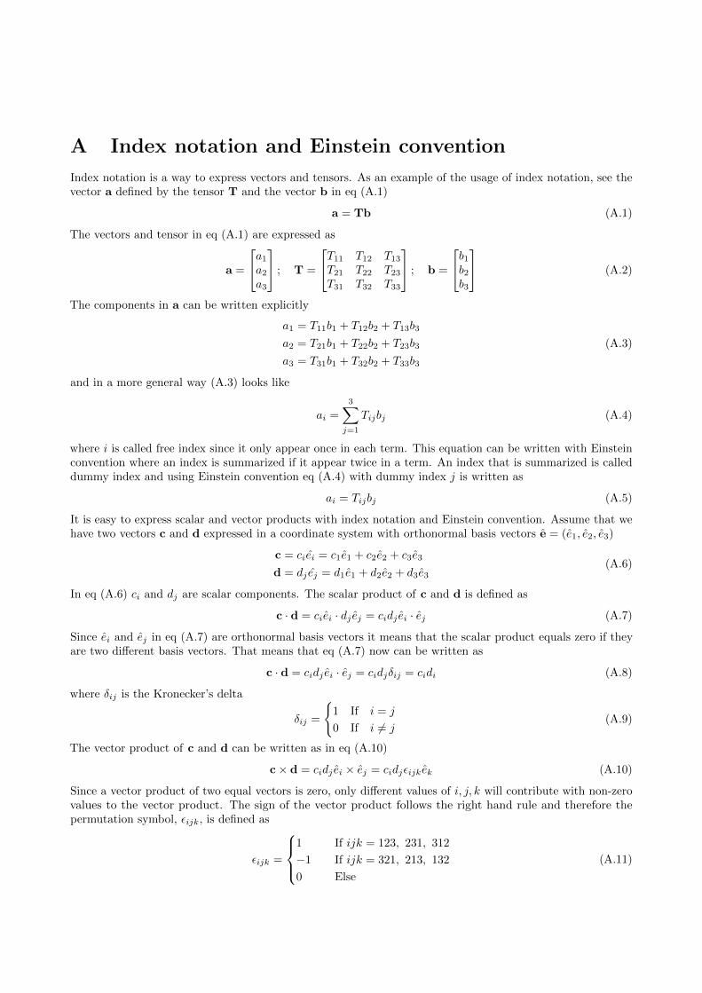
A Index notation and Einstein convention
Index notation is a way to express vectors and tensors. As an example of the usage of index notation, see thevector a defined by the tensor T and the vector b in eq (A.1)
a = Tb (A.1)
The vectors and tensor in eq (A.1) are expressed as
a =
a1
a2
a3
; T =
T11 T12 T13
T21 T22 T23
T31 T32 T33
; b =
b1b2b3
(A.2)
The components in a can be written explicitly
a1 = T11b1 + T12b2 + T13b3
a2 = T21b1 + T22b2 + T23b3
a3 = T31b1 + T32b2 + T33b3
(A.3)
and in a more general way (A.3) looks like
ai =
3∑j=1
Tijbj (A.4)
where i is called free index since it only appear once in each term. This equation can be written with Einsteinconvention where an index is summarized if it appear twice in a term. An index that is summarized is calleddummy index and using Einstein convention eq (A.4) with dummy index j is written as
ai = Tijbj (A.5)
It is easy to express scalar and vector products with index notation and Einstein convention. Assume that wehave two vectors c and d expressed in a coordinate system with orthonormal basis vectors e = (e1, e2, e3)
c = ciei = c1e1 + c2e2 + c3e3
d = dj ej = d1e1 + d2e2 + d3e3
(A.6)
In eq (A.6) ci and dj are scalar components. The scalar product of c and d is defined as
c · d = ciei · dj ej = cidj ei · ej (A.7)
Since ei and ej in eq (A.7) are orthonormal basis vectors it means that the scalar product equals zero if theyare two different basis vectors. That means that eq (A.7) now can be written as
c · d = cidj ei · ej = cidjδij = cidi (A.8)
where δij is the Kronecker’s delta
δij =
{1 If i = j
0 If i 6= j(A.9)
The vector product of c and d can be written as in eq (A.10)
c× d = cidj ei × ej = cidjεijkek (A.10)
Since a vector product of two equal vectors is zero, only different values of i, j, k will contribute with non-zerovalues to the vector product. The sign of the vector product follows the right hand rule and therefore thepermutation symbol, εijk, is defined as
εijk =
1 If ijk = 123, 231, 312
−1 If ijk = 321, 213, 132
0 Else
(A.11)
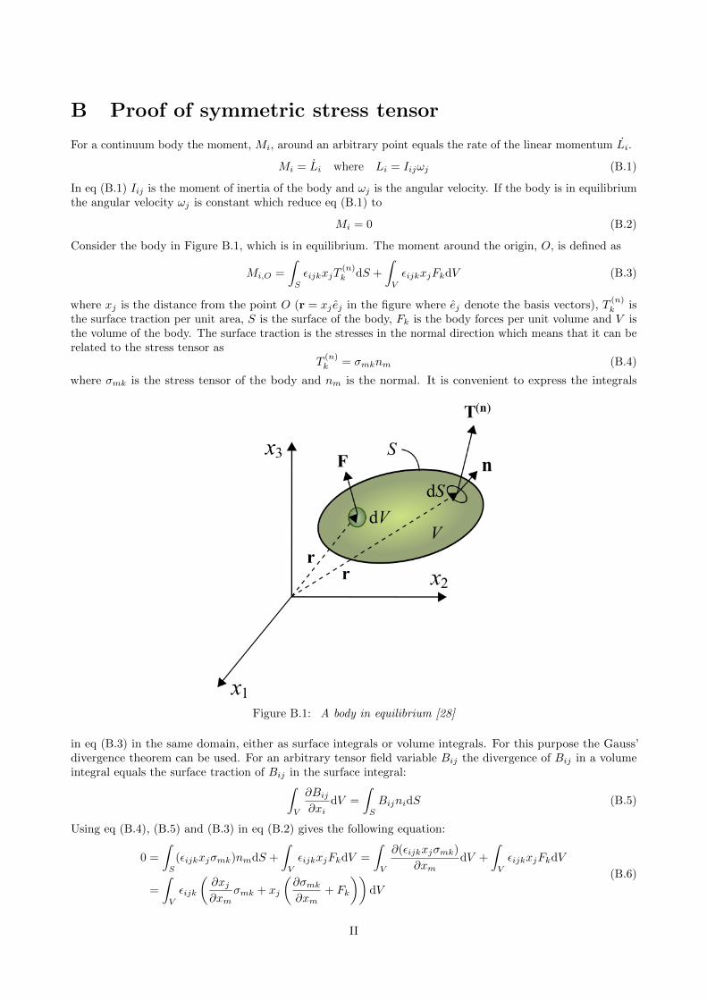
B Proof of symmetric stress tensor
For a continuum body the moment, Mi, around an arbitrary point equals the rate of the linear momentum Li.
Mi = Li where Li = Iijωj (B.1)
In eq (B.1) Iij is the moment of inertia of the body and ωj is the angular velocity. If the body is in equilibriumthe angular velocity ωj is constant which reduce eq (B.1) to
Mi = 0 (B.2)
Consider the body in Figure B.1, which is in equilibrium. The moment around the origin, O, is defined as
Mi,O =
∫S
εijkxjT(n)k dS +
∫V
εijkxjFkdV (B.3)
where xj is the distance from the point O (r = xj ej in the figure where ej denote the basis vectors), T(n)k is
the surface traction per unit area, S is the surface of the body, Fk is the body forces per unit volume and V isthe volume of the body. The surface traction is the stresses in the normal direction which means that it can berelated to the stress tensor as
T(n)k = σmknm (B.4)
where σmk is the stress tensor of the body and nm is the normal. It is convenient to express the integrals
Figure B.1: A body in equilibrium [28]
in eq (B.3) in the same domain, either as surface integrals or volume integrals. For this purpose the Gauss’divergence theorem can be used. For an arbitrary tensor field variable Bij the divergence of Bij in a volumeintegral equals the surface traction of Bij in the surface integral:∫
V
∂Bij∂xi
dV =
∫S
BijnidS (B.5)
Using eq (B.4), (B.5) and (B.3) in eq (B.2) gives the following equation:
0 =
∫S
(εijkxjσmk)nmdS +
∫V
εijkxjFkdV =
∫V
∂(εijkxjσmk)
∂xmdV +
∫V
εijkxjFkdV
=
∫V
εijk
(∂xj∂xm
σmk + xj
(∂σmk∂xm
+ Fk
))dV
(B.6)
II
Here the second term in the final expression contains the governing equation for conservation of momentum,which equals zero at equilibrium conditions. Also it should be noted that the partial derivative in the first termequals zero if j 6= m and equals unity if j = m. Therefore this term equals the Kronecker’s delta, δjm. Theonly non-zero terms appears when j = m and eq (B.6) is now written as:
0 =
∫V
εijkσjkdV (B.7)
The equation is valid for an arbitrary volume V which means that
εijkσjk = 0 (B.8)
must be fulfilled. Doing the summation gives three relations
ε123σ23 + ε132σ32 = σ23 − σ32 = 0 (B.9)
ε213σ13 + ε231σ31 = σ13 − σ31 = 0 (B.10)
ε312σ12 + ε321σ21 = σ12 − σ21 = 0 (B.11)
This can generally be written asσij = σji (B.12)
which proofs that the stress tensor, σij is symmetric.
III
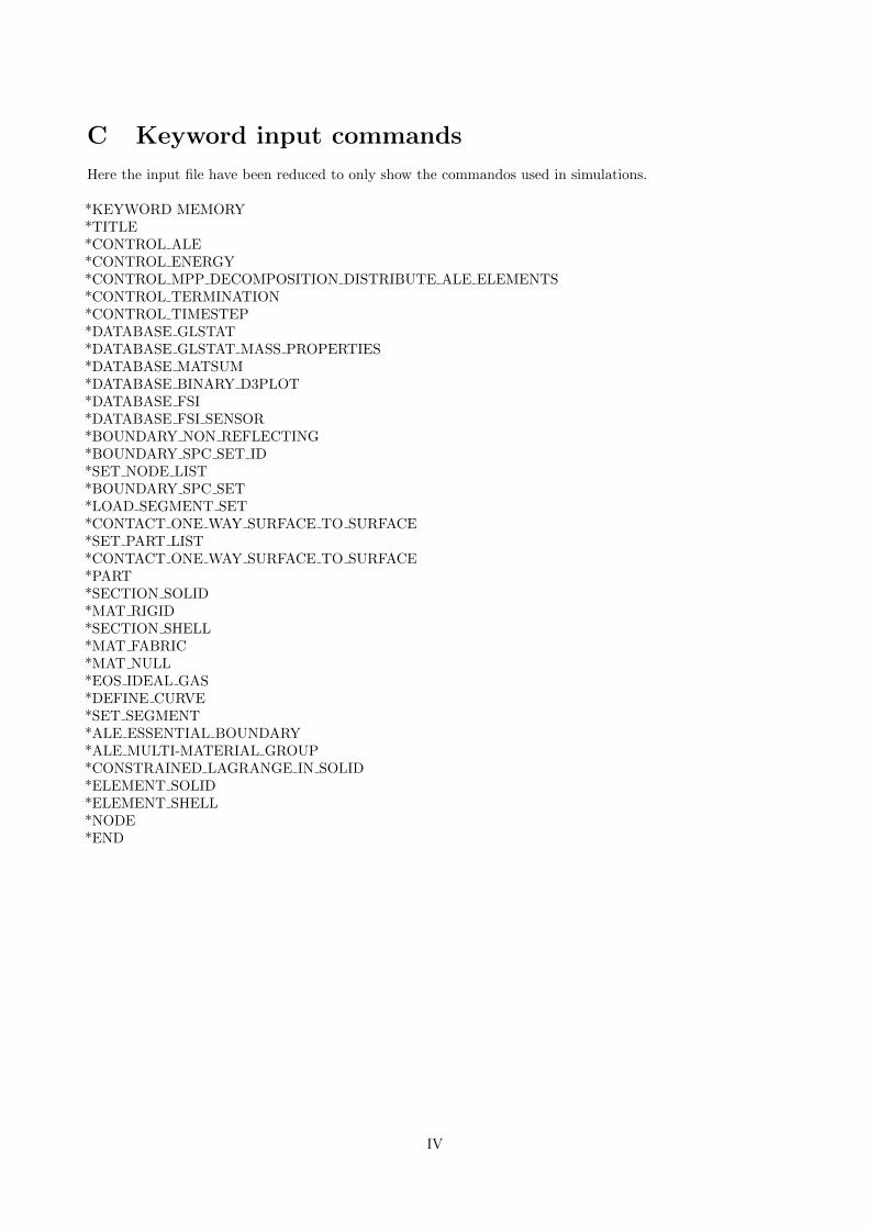
C Keyword input commands
Here the input file have been reduced to only show the commandos used in simulations.
*KEYWORD MEMORY*TITLE*CONTROL ALE*CONTROL ENERGY*CONTROL MPP DECOMPOSITION DISTRIBUTE ALE ELEMENTS*CONTROL TERMINATION*CONTROL TIMESTEP*DATABASE GLSTAT*DATABASE GLSTAT MASS PROPERTIES*DATABASE MATSUM*DATABASE BINARY D3PLOT*DATABASE FSI*DATABASE FSI SENSOR*BOUNDARY NON REFLECTING*BOUNDARY SPC SET ID*SET NODE LIST*BOUNDARY SPC SET*LOAD SEGMENT SET*CONTACT ONE WAY SURFACE TO SURFACE*SET PART LIST*CONTACT ONE WAY SURFACE TO SURFACE*PART*SECTION SOLID*MAT RIGID*SECTION SHELL*MAT FABRIC*MAT NULL*EOS IDEAL GAS*DEFINE CURVE*SET SEGMENT*ALE ESSENTIAL BOUNDARY*ALE MULTI-MATERIAL GROUP*CONSTRAINED LAGRANGE IN SOLID*ELEMENT SOLID*ELEMENT SHELL*NODE*END
IV