geometric study of lagrangian and eulerian structures in ...geometric study of lagrangian and...

J. Fluid Mech. (2011), vol. 674, pp. 67–92. c© Cambridge University Press 2011

doi:10.1017/S0022112010006427

67

Geometric study of Lagrangian and Eulerianstructures in turbulent channel flow

YUE YANG† AND D. I. PULLINGraduate Aerospace Laboratories, 205-45, California Institute of Technology,

Pasadena, CA 91125, USA

(Received 9 August 2010; revised 7 December 2010; accepted 13 December 2010;

first published online 2 March 2011)

We report the detailed multi-scale and multi-directional geometric study of bothevolving Lagrangian and instantaneous Eulerian structures in turbulent channel flowat low and moderate Reynolds numbers. The Lagrangian structures (material surfaces)are obtained by tracking the Lagrangian scalar field, and Eulerian structures areextracted from the swirling strength field at a time instant. The multi-scale and multi-directional geometric analysis, based on the mirror-extended curvelet transform, isdeveloped to quantify the geometry, including the averaged inclination and sweepangles, of both structures at up to eight scales ranging from the half-height δ of thechannel to several viscous length scales δν . Here, the inclination angle is on the planeof the streamwise and wall-normal directions, and the sweep angle is on the plane ofstreamwise and spanwise directions. The results show that coherent quasi-streamwisestructures in the near-wall region are composed of inclined objects with averagedinclination angle 35◦–45◦, averaged sweep angle 30◦–40◦ and characteristic scale 20δν ,and ‘curved legs’ with averaged inclination angle 20◦–30◦, averaged sweep angle 15◦–30◦ and length scale 5δν–10δν . The temporal evolution of Lagrangian structures showsincreasing inclination and sweep angles with time, which may correspond to the liftingprocess of near-wall quasi-streamwise vortices. The large-scale structures that appearto be composed of a number of individual small-scale objects are detected using cross-correlations between Eulerian structures with large and small scales. These packetsare located at the near-wall region with the typical height 0.25δ and may extend over10δ in the streamwise direction in moderate-Reynolds-number, long channel flows. Inaddition, the effects of the Reynolds number and comparisons between Lagrangianand Eulerian structures are discussed.

Key words: boundary layer structure, turbulence theory, turbulent boundary layers.

1. IntroductionCoherent motions or structures with identifiable tube-like shapes that appear to

contain concentrated vorticity have been extensively observed and reported fromvisualizations of laboratory experiments and numerical simulations of wall-boundedturbulence. Although the role played by turbulent coherent, near-wall structures isstill not fully understood, over the past several decades many studies have providedevidence supporting the hypothesis that these structures constitute, in some statisticalsense, basic elemental vortices that participate in the dynamics of near-wall turbulence

† Email address for correspondence: [email protected]

68 Y. Yang and D. I. Pullin

and are important for drag reduction, turbulent control and other applications (seeRobinson 1991; Panton 2001). In addition, it has been argued that the scaling lawsand high-order statistics of the mean velocity and velocity fluctuations are influencedby inclined, coherent structures in the near-wall region (see Adrian 2007) and large-scale structures in the outer layer (see Hutchins & Marusic 2007). In what follows, wewill generally use the term ‘quasi-streamwise vortices’, which has been hypothesizedin the cited references, to denote individual inclined structures or objects that exist innear-wall turbulence. In the present work, we describe geometry-based metrics thatfurther supports the existence of these structures.

Both Lagrangian- and Eulerian-based approaches have been used to study wallturbulence. Lagrangian methods typically track trajectories of fluid particles, oftenusing visualization techniques. Particle tracers such as hydrogen bubbles (e.g. Klineet al. 1967) or passive scalars such as smoke or dye (e.g. Head & Bandyopadhyay1981) show evolving flow structures. These visual studies revealed rich geometriesin turbulent structures but remain mainly qualitative (Robinson 1991). Eulerianmethodologies benefited from the development of direct numerical simulation (DNS)(e.g. Kim, Moin & Moser 1987) and experimental particle-image velocimetry (PIV)(e.g. Liu et al. 1991) which provide full, two- or three-dimensional instantaneousvelocity fields. The Eulerian structures are usually extracted using either iso-surfacesof vorticity magnitude or popular vortex identification criteria (e.g. Hunt, Wray &Moin 1988; Chong, Perry & Cantwell 1990; Jeong & Hussain 1995).

Major observations on coherent structures in wall turbulence include that thestreamwise velocity field close to the wall is organized into alternating narrowstreaks of high- and low-speed velocity (Kline et al. 1967) and that candidatehairpin- or Λ-like vortices may exist in the logarithmic region, while the turbulentmotion appears to be less active in the outer layer. The conceptual model of thehairpin vortex was developed by Theodorsen (1952) and supported by experiment(Head & Bandyopadhyay 1981) and computation visualizations (Moin & Kim 1982).The modern model of the hairpin vortex is usually described as a combinationeddy composed of a hairpin body and two relatively short counter-rotating quasi-streamwise vortices that create low-speed streaks in the buffer layer (Adrian 2007).Furthermore, recent DNS and PIV studies provide evidence that hairpin-like structurescan autogenerate to form packets that occupy a significant volume fraction of theboundary layer (e.g. Zhou et al. 1999).

Although observation of Eulerian structures can perhaps elucidate turbulenceflow physics at a time instant, the Lagrangian approach seems better suited forinvestigation of the temporal evolution of turbulent coherent structures and theirdynamical role in turbulent transition and mixing. This issue was discussed by Green,Rowley & Haller (2007) who showed the evolution of single vortex-like structures intoa packet of similar structures in turbulent channel flow by identifying ‘Lagrangiancoherent structures’ (Haller 2001). Yang, Pullin & Bermejo-Moreno (2010) illustratedand quantified the evolutionary geometry in the breakdown of initially large-scaleLagrangian structures in isotropic turbulence using a multi-scale geometric analysis.

Consensus on the accepted geometry of vortical structures in wall-boundedturbulence remains elusive. From flow visualization studies of the turbulent boundarylayer, Falco (1977) showed that large-scale structures of the smoke concentrationfield, with typical length scales from δ to 3δ, inclined to the wall at a characteristicangle 20◦–25◦, while Head & Bandyopadhyay (1981) measured an inclination angle40◦–50◦ for candidate hairpins. Using large-eddy simulation (LES) and correlationstudies, Moin & Kim (1985) obtained a most probable inclination angle of local

Geometric study of structures in turbulent channel flow 69

vorticity vector as 45◦, while Honkan & Andreopoulos (1997) found that the vorticityis inclined at 35◦ from multi-probe hot wire measurements. Using PIV experimentsand statistical tools Ganapathisubramani, Longmire & Marusic (2006) identifiedindividual vortex cores most frequently inclined at 45◦. The model developed byBandyopadhyay (1980) gives that the inclination angle of candidate hairpin packetsis 18◦. Christensen & Adrian (2001) found an inclination angle of 12◦–13◦ for theenvelope of a series of swirling motions. In contrast, contour-dynamics simulation(Pullin 1981) of a two-dimensional, uniform vorticity layer adjacent to a wall showedinclined structures that resemble flow features observed in the smoke visualization(Falco 1977) of the interface between turbulent and non-turbulent fluid in the outerpart of a turbulent boundary layer. This suggests that at least these outer featuresmay not be generated entirely by three-dimensional effects. Open questions remainwhose resolution may depend on the scale of structures, Reynolds numbers and theusage of Lagrangian or Eulerian methods in investigations.

The geometry of eddies is also of interest for structure-based models of near-wall turbulence. Predictive models have been developed, based on the attached eddyhypothesis (Townsend 1976), that utilize random superpositions of hierarchies ofeither hairpins (Perry & Chong 1982; Perry, Henbest & Chong 1986; Perry & Marusic1995) or hairpin packets (Marusic 2001). A particular geometry or shape of hairpinor Λ-like vortices is assumed. Additionally, geometrical issues may inform near-wall,subgrid-scale modelling for LES based on small-scale, vortical structures (Chung &Pullin 2009). The existence of coherent structures with characteristic geometric featuresmay suggest a possible sparse representation for reconstructing a whole channelflow with a greatly reduced number of optimal basis functions utilizing either awavelet- or curvelet-based extraction method (e.g. Okamoto et al. 2007; Ma et al.2009).

In the present work, the multi-scale geometric analysis of both Lagrangian andEulerian structures (Bermejo-Moreno & Pullin 2008; Yang et al. 2010) in isotropicturbulence is extended to turbulent channel flow by introducing the multi-directionaldecomposition and mirror-extended data. The extended geometric analysis, which isbased on the mirror-extended curvelet transform (see Candes et al. 2006; Demanet &Ying 2007), will include both multi-scale and multi-directional decompositions ofa specific scalar field with non-periodic boundary conditions in wall turbulence.This provides quantitative statistics on the orientation of turbulent structures atdifferent locations, scales and Reynolds numbers. Phenomena in wall turbulence tobe investigated include the following: first, the detailed geometry of quasi-streamwisevortices and other structures in the near-wall region (about 5δν to 0.3δ); second, thestructural evolution of near-wall vortices, with initially almost spanwise orientationwithin the buffer region very close to the wall, into possible Λ-like or hairpin vorticesat a larger wall distance; third, the existence and geometry of packets, based onstatistical evidence obtained from multi-scale analysis.

We begin in § 2 by giving a simulation overview for the DNS, using a spectralmethod, and the computation of Lagrangian fields with the backward-particle-tracking method. In § 3, a systematic framework is introduced to quantify geometriesincluding averaged inclination and sweep angles of flow structures at multiple scales.Section 4 shows the application of the multi-scale and multi-directional geometricanalysis to investigate the geometry of Lagrangian structures at different length scalesin time evolution. In § 5 we investigate the geometry of multi-scale, Eulerian structuresand provide statistical evidence supporting the formation of structure packets. Finally,some conclusions are drawn in § 6.


xy

z

U

(0, 0, 0)

(Lx, Ly, Lz)

α+

α−

β+β− x – y plane

x – z plane

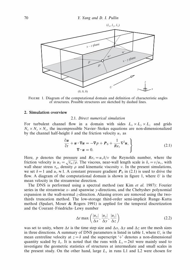
Figure 1. Diagram of the computational domain and definition of characteristic anglesof structures. Possible structures are sketched by dashed lines.

2. Simulation overview2.1. Direct numerical simulation

For turbulent channel flow in a domain with sides Lx ×Ly ×Lz and gridsNx ×Ny ×Nz, the incompressible Navier–Stokes equations are non-dimensionalizedby the channel half-height δ and the friction velocity uτ as

∂u∂t

+ u · ∇u = −∇p + P0 +1

Reτ

∇2u,

∇ · u = 0.

⎫⎬⎭ (2.1)

Here, p denotes the pressure and Reτ = uτ δ/ν the Reynolds number, where thefriction velocity is uτ =

√τw/ρ. The viscous, near-wall length scale is δν = ν/uτ , with

wall shear stress τw , density ρ and kinematic viscosity ν. In the present simulations,we set δ =1 and uτ ≈ 1. A constant pressure gradient P0 in (2.1) is used to drive theflow. A diagram of the computational domain is shown in figure 1, where U is themean velocity in the streamwise direction.

The DNS is performed using a spectral method (see Kim et al. 1987): Fourierseries in the streamwise x- and spanwise y-directions, and the Chebyshev polynomialexpansion in the wall-normal z-direction. Aliasing errors are removed using the two-thirds truncation method. The low-storage third-order semi-implicit Runge–Kuttamethod (Spalart, Moser & Rogers 1991) is applied for the temporal discretizationand the Courant–Friedrichs–Lewy number

�t max

(|ux |�x

,|uy |�y

,|uz|�z

)(2.2)

was set to unity, where �t is the time step size and �x, �y and �z are the mesh sizesin three directions. A summary of DNS parameters is listed in table 1, where Uc is themean centreline velocity at z = δ and the superscript ‘+’ denotes a non-dimensionalquantity scaled by δν . It is noted that the runs with Lx = 2πδ were mainly used toinvestigate the geometric statistics of structures at intermediate and small scales inthe present study. On the other hand, large Lx in runs L1 and L2 were chosen for


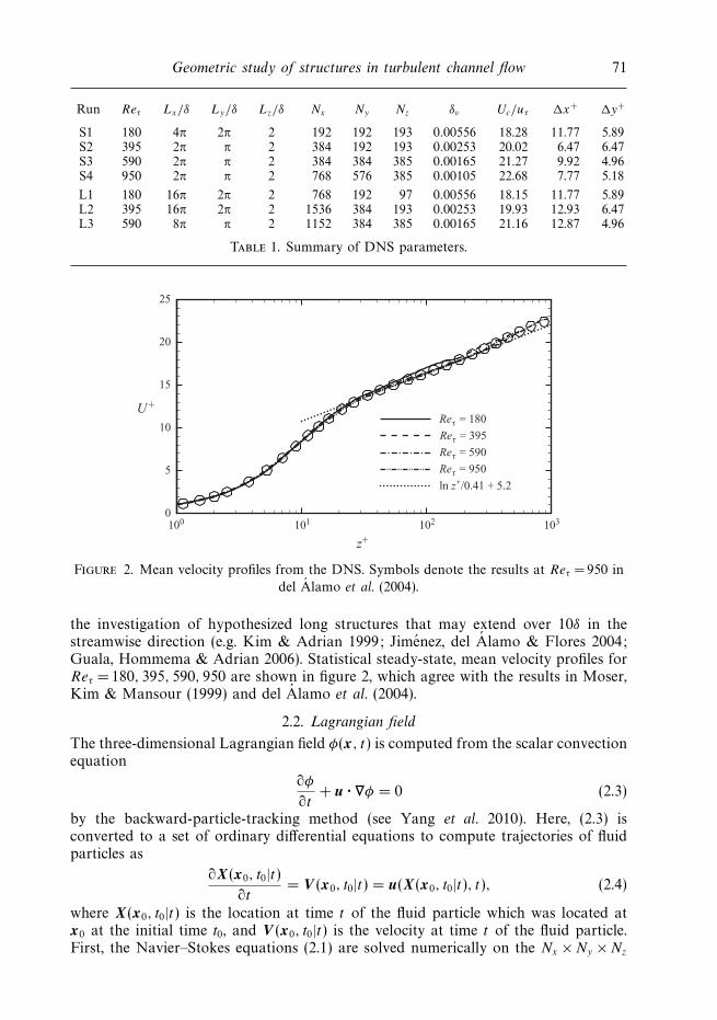
Run Reτ Lx/δ Ly/δ Lz/δ Nx Ny Nz δν Uc/uτ �x+ �y+

S1 180 4π 2π 2 192 192 193 0.00556 18.28 11.77 5.89S2 395 2π π 2 384 192 193 0.00253 20.02 6.47 6.47S3 590 2π π 2 384 384 385 0.00165 21.27 9.92 4.96S4 950 2π π 2 768 576 385 0.00105 22.68 7.77 5.18

L1 180 16π 2π 2 768 192 97 0.00556 18.15 11.77 5.89L2 395 16π 2π 2 1536 384 193 0.00253 19.93 12.93 6.47L3 590 8π π 2 1152 384 385 0.00165 21.16 12.87 4.96

Table 1. Summary of DNS parameters.

100 101 102 1030

5

10

15

20

25

Reτ = 180

Reτ = 395

Reτ = 590

Reτ = 950

U +

z+

ln z+/0.41 + 5.2

Figure 2. Mean velocity profiles from the DNS. Symbols denote the results at Reτ = 950 in

del Alamo et al. (2004).

the investigation of hypothesized long structures that may extend over 10δ in thestreamwise direction (e.g. Kim & Adrian 1999; Jimenez, del Alamo & Flores 2004;Guala, Hommema & Adrian 2006). Statistical steady-state, mean velocity profiles forReτ = 180, 395, 590, 950 are shown in figure 2, which agree with the results in Moser,Kim & Mansour (1999) and del Alamo et al. (2004).

2.2. Lagrangian field

The three-dimensional Lagrangian field φ(x, t) is computed from the scalar convectionequation

∂φ

∂t+ u · ∇φ = 0 (2.3)

by the backward-particle-tracking method (see Yang et al. 2010). Here, (2.3) isconverted to a set of ordinary differential equations to compute trajectories of fluidparticles as

∂X(x0, t0|t)∂t

= V (x0, t0|t) = u(X(x0, t0|t), t), (2.4)

where X(x0, t0|t) is the location at time t of the fluid particle which was located atx0 at the initial time t0, and V (x0, t0|t) is the velocity at time t of the fluid particle.First, the Navier–Stokes equations (2.1) are solved numerically on the Nx ×Ny ×Nz


grid in some time interval from t0 to t > t0, and the full Eulerian velocity field issaved on disk in this simulation period. The time increment is selected to capturethe finest resolved scales in the velocity field. At time t at the end of the solutionperiod, particles are placed at the uniform grid points of NL

x ×NLy ×NL

z . Presently,the resolution of the Lagrangian field is two times that of the velocity field in orderto capture fine-scale Lagrangian structures in the evolution (Yang et al. 2010). Then,particles are released and their trajectories calculated by solving (2.4) backwards intime. A three-dimensional, fourth-order Lagrangian interpolation scheme was usedto calculate fluid velocity at the particle location. The trajectory of each particle wasthen obtained using an explicit, second-order Adams–Bashforth scheme. For eachparticle the backward tracking is performed from t to the initial time t0 with thereversed Eulerian velocity fields saved previously. After the backward tracking, initiallocations of particles x0 can be obtained. From a given initial condition consisting ofa smooth Lagrangian field φ(x0, t0), we can then obtain φ(x, t) on the Cartesian gridby a simple mapping with Lagrangian coordinates

φ(x, t) = φ(X(x0, t0|t), t)←→ φ(x0, t0). (2.5)

3. Multi-scale and multi-directional methodology3.1. Multi-scale and multi-directional filter based on curvelet transform

When a scalar field has preferential orientations, e.g. streaks in an image, the Fouriertransform of the scalar field should have high intensities at some particular localizedregions in Fourier space. Thus, the directional decomposition of the scalar field canbe obtained by spectral directional/fan filters, which have been used in computervision, seismology and image compression (e.g. Bamberger & Smith 1992). Presently,to obtain statistical, geometric information on preferential orientations in a three-dimensional field at different scales, we apply a multi-scale directional filter basedon the curvelet transform (see Candes et al. 2006, and references therein) to asequence of two-dimensional plane-cuts and then compute the angular spectrum andcorresponding averaged angles.

An arbitrary two-dimensional scalar field ϕ(x) can be represented by the Fourierexpansion

ϕ(x) =∑

k

ϕ(k) eik·x, (3.1)

where x = (x1, x2), k = (k1, k2) and the Fourier coefficient

ϕ(k) =1

2π

∫ϕ(x) e−ik·x dx. (3.2)

In the numerical implementation, ϕ(x1, x2) is discretized on a rectangular domainof side L1×L2 using an N1×N2 grid with indices (n1, n2) in physical space. Thecorresponding Fourier space can be discretized on the grid N1×N2 with indices(m1, m2). The discrete Fourier transform (DFT) and inverse DFT of ϕ(x) are

ϕ(k1,m1, k2,m2

) =1

N1

1

N2

N1−1∑n1=0

N2−1∑n2=0

ϕ(x1,n1, x2,n2

) exp[−i(k1,m1x1,n1

+ k2,m2x2,n2

)], (3.3)

ϕ(x1,n1, x2,n2

) =

N1−1∑m1=0

N2−1∑m2=0

ϕ(k1,m1, k2,m2

) exp[i(k1,m1x1,n1

+ k2,m2x2,n2

)], (3.4)


respectively, with

ki,mi= mi�ki, xi,ni

= ni�xi, �xi = Li/Ni, �ki = 2π/Li. (3.5)

A filtered ϕ(x) at scale j and along the direction l can then be extracted from ϕ(k)in Fourier space by the frequency window function

Uj (r, θ) = 2−3j/4W (2−j r)V (tl(θ)), (3.6)

in polar coordinates (r, θ) with r =√

k21 + k2

2 and θ = arctan(k2/k1). The frequencywindow function Uj (r, θ) is based on the curvelet transform (Candes et al. 2006),which is a combination of the radial window function (e.g. Ma et al. 2009)

W (r) =

⎧⎪⎪⎨⎪⎪⎩

cos(πµ(5− 6r)/2), 2/3 � r � 5/6,

1, 5/6 � r � 4/3,

cos(πµ(3r − 4)/2), 4/3 � r � 5/3,

0, else,

(3.7)

and the angular window function

V (tl) =

⎧⎨⎩

1, |tl |� 1/3,

cos(πµ(3|tl | − 4)/2), 4/3 � tl � 5/3,

0, else,

(3.8)

with the smoothing function µ(x) = 3x2 − 2x3 satisfying

µ(x) =

{1, x � 0,

0, x � 1,µ(x) + µ(1− x) = 1. (3.9)

Both radial and angular window functions satisfy the admissibility conditions:

∞∑r=−∞

W 2(2j r) = 1, r > 0, (3.10)

∞∑tl=−∞

V 2(tl) = 1, tl ∈ �. (3.11)

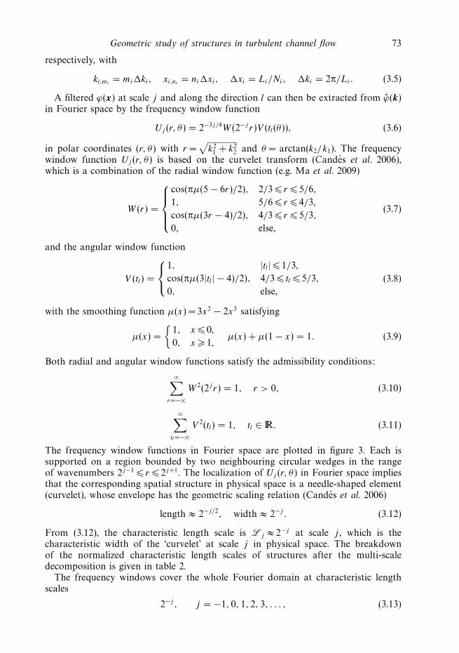
The frequency window functions in Fourier space are plotted in figure 3. Each issupported on a region bounded by two neighbouring circular wedges in the rangeof wavenumbers 2j−1 � r � 2j+1. The localization of Uj (r, θ) in Fourier space impliesthat the corresponding spatial structure in physical space is a needle-shaped element(curvelet), whose envelope has the geometric scaling relation (Candes et al. 2006)

length ≈ 2−j/2, width ≈ 2−j . (3.12)

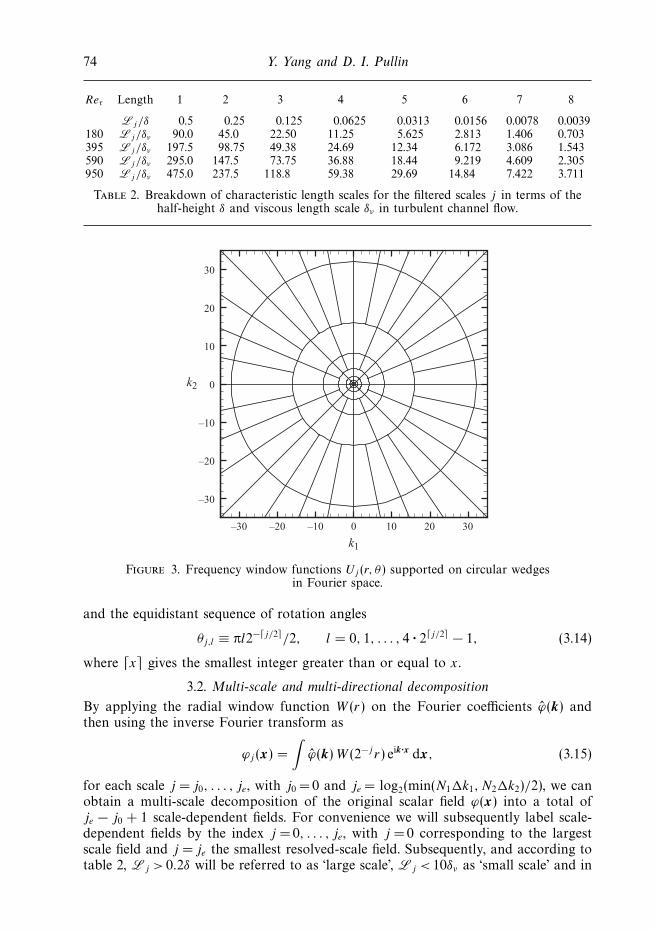
From (3.12), the characteristic length scale is Lj ≈ 2−j at scale j , which is thecharacteristic width of the ‘curvelet’ at scale j in physical space. The breakdownof the normalized characteristic length scales of structures after the multi-scaledecomposition is given in table 2.

The frequency windows cover the whole Fourier domain at characteristic lengthscales

2−j , j = −1, 0, 1, 2, 3, . . . , (3.13)


Reτ Length 1 2 3 4 5 6 7 8

Lj /δ 0.5 0.25 0.125 0.0625 0.0313 0.0156 0.0078 0.0039180 Lj /δν 90.0 45.0 22.50 11.25 5.625 2.813 1.406 0.703395 Lj /δν 197.5 98.75 49.38 24.69 12.34 6.172 3.086 1.543590 Lj /δν 295.0 147.5 73.75 36.88 18.44 9.219 4.609 2.305950 Lj /δν 475.0 237.5 118.8 59.38 29.69 14.84 7.422 3.711

Table 2. Breakdown of characteristic length scales for the filtered scales j in terms of thehalf-height δ and viscous length scale δν in turbulent channel flow.

–30 –20 –10 0 10 20 30

–30

–20

–10

0

10

20

30

k2

k1

Figure 3. Frequency window functions Uj (r, θ ) supported on circular wedgesin Fourier space.

and the equidistant sequence of rotation angles

θj,l ≡ πl2−�j/2�/2, l = 0, 1, . . . , 4 · 2�j/2� − 1, (3.14)

where �x� gives the smallest integer greater than or equal to x.

3.2. Multi-scale and multi-directional decomposition

By applying the radial window function W (r) on the Fourier coefficients ϕ(k) andthen using the inverse Fourier transform as

ϕj (x) =

∫ϕ(k) W (2−j r) eik·x dx, (3.15)

for each scale j = j0, . . . , je, with j0 = 0 and je = log2(min(N1�k1, N2�k2)/2), we canobtain a multi-scale decomposition of the original scalar field ϕ(x) into a total ofje − j0 + 1 scale-dependent fields. For convenience we will subsequently label scale-dependent fields by the index j = 0, . . . , je, with j = 0 corresponding to the largestscale field and j = je the smallest resolved-scale field. Subsequently, and according totable 2, Lj > 0.2δ will be referred to as ‘large scale’, Lj < 10δν as ‘small scale’ and in


x1 x1

x2

�θ

x2

〈�θ〉j−

〈�θ〉j+

(a) (b)

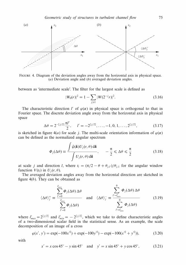
Figure 4. Diagram of the deviation angles away from the horizontal axis in physical space.(a) Deviation angle and (b) averaged deviation angles.

between as ‘intermediate scale’. The filter for the largest scale is defined as

|W0(r)|2 = 1−∑j�1

|W (2−j r)|2. (3.16)

The characteristic direction l′ of ϕ(x) in physical space is orthogonal to that inFourier space. The discrete deviation angle away from the horizontal axis in physicalspace

�θ = 2−�j/2�πl′

2, l′ = −2�j/2�, . . . ,−1, 0, 1, . . . , 2�j/2�, (3.17)

is sketched in figure 4(a) for scale j . The multi-scale orientation information of ϕ(x)can be defined as the normalized angular spectrum

Φj (�θ) ≡

∫ϕ(k)Uj (r, θ) dk∫

Uj (r, θ) dk, − π

2� �θ �

π

2(3.18)

at scale j and direction l, where tl = (π/2 − θ + θj,l′)/θj,1 for the angular windowfunction V (tl) in Uj (r, θ).

The averaged deviation angles away from the horizontal direction are sketched infigure 4(b). They can be obtained as

〈�θ〉+j ≡

l′max∑l′=0

Φj (�θ) �θ

l′max∑l′=0

Φj (�θ)

and 〈�θ〉−j ≡

0∑l′=l′min

Φj (�θ) �θ

0∑l′=l′min

Φj (�θ)

(3.19)

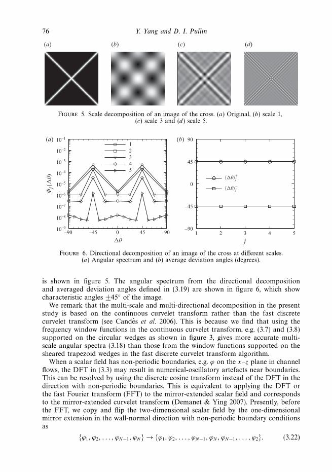
where l′max = 2�j/2� and l′min = − 2�j/2�, which we take to define characteristic anglesof a two-dimensional scalar field in the statistical sense. As an example, the scaledecomposition of an image of a cross

ϕ(x ′, y ′) = exp(−100x ′2) + exp(−100y ′2)− exp(−100(x ′2 + y ′2)), (3.20)

with

x ′ = x cos 45◦ − y sin 45◦ and y ′ = x sin 45◦ + y cos 45◦, (3.21)


(a) (b) (c) (d)

Figure 5. Scale decomposition of an image of the cross. (a) Original, (b) scale 1,(c) scale 3 and (d) scale 5.

–90 –45 0 45 9010–9

10–8

10–7

10–6

10–5

10–4

10–3

10–2

10–1

Φj(

�θ)

12345

1 2 3 4 5–90

–45

0

45

90

j

(a) (b)

�θ

〈�θ〉j−

〈�θ〉j+

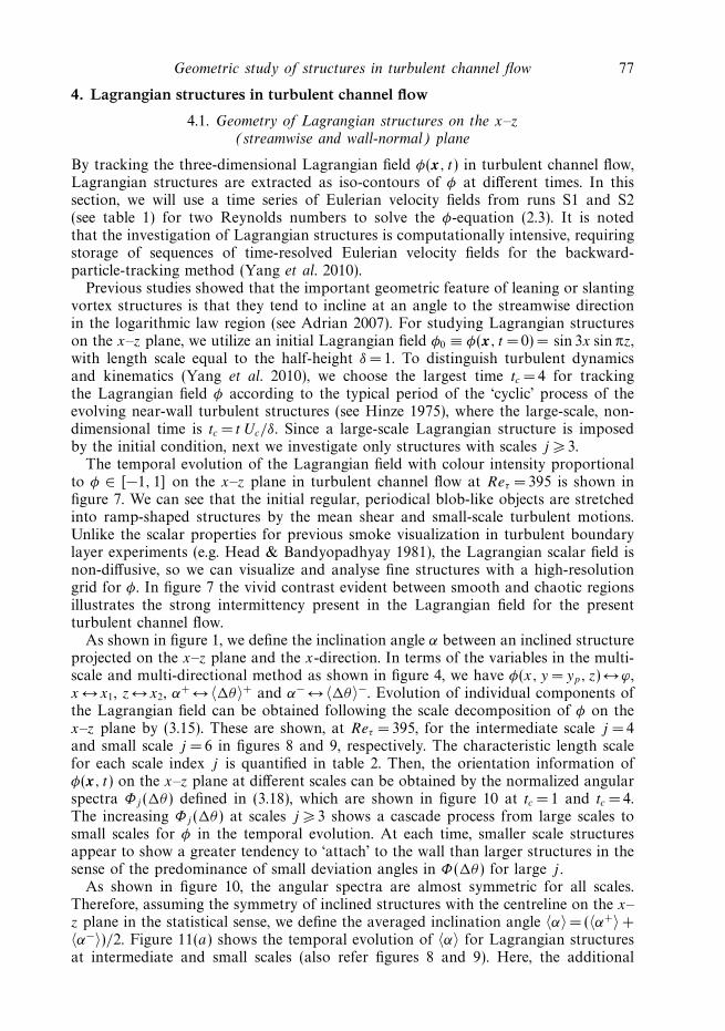
Figure 6. Directional decomposition of an image of the cross at different scales.(a) Angular spectrum and (b) average deviation angles (degrees).

is shown in figure 5. The angular spectrum from the directional decompositionand averaged deviation angles defined in (3.19) are shown in figure 6, which showcharacteristic angles ±45◦ of the image.

We remark that the multi-scale and multi-directional decomposition in the presentstudy is based on the continuous curvelet transform rather than the fast discretecurvelet transform (see Candes et al. 2006). This is because we find that using thefrequency window functions in the continuous curvelet transform, e.g. (3.7) and (3.8)supported on the circular wedges as shown in figure 3, gives more accurate multi-scale angular spectra (3.18) than those from the window functions supported on thesheared trapezoid wedges in the fast discrete curvelet transform algorithm.

When a scalar field has non-periodic boundaries, e.g. ϕ on the x–z plane in channelflows, the DFT in (3.3) may result in numerical-oscillatory artefacts near boundaries.This can be resolved by using the discrete cosine transform instead of the DFT in thedirection with non-periodic boundaries. This is equivalent to applying the DFT orthe fast Fourier transform (FFT) to the mirror-extended scalar field and correspondsto the mirror-extended curvelet transform (Demanet & Ying 2007). Presently, beforethe FFT, we copy and flip the two-dimensional scalar field by the one-dimensionalmirror extension in the wall-normal direction with non-periodic boundary conditionsas

{ϕ1, ϕ2, . . . , ϕN−1, ϕN} → {ϕ1, ϕ2, . . . , ϕN−1, ϕN, ϕN−1, . . . , ϕ2}. (3.22)


4. Lagrangian structures in turbulent channel flow

4.1. Geometry of Lagrangian structures on the x–z

(streamwise and wall-normal) plane

By tracking the three-dimensional Lagrangian field φ(x, t) in turbulent channel flow,Lagrangian structures are extracted as iso-contours of φ at different times. In thissection, we will use a time series of Eulerian velocity fields from runs S1 and S2(see table 1) for two Reynolds numbers to solve the φ-equation (2.3). It is notedthat the investigation of Lagrangian structures is computationally intensive, requiringstorage of sequences of time-resolved Eulerian velocity fields for the backward-particle-tracking method (Yang et al. 2010).

Previous studies showed that the important geometric feature of leaning or slantingvortex structures is that they tend to incline at an angle to the streamwise directionin the logarithmic law region (see Adrian 2007). For studying Lagrangian structureson the x–z plane, we utilize an initial Lagrangian field φ0 ≡ φ(x, t =0)= sin 3x sin πz,with length scale equal to the half-height δ =1. To distinguish turbulent dynamicsand kinematics (Yang et al. 2010), we choose the largest time tc =4 for trackingthe Lagrangian field φ according to the typical period of the ‘cyclic’ process of theevolving near-wall turbulent structures (see Hinze 1975), where the large-scale, non-dimensional time is tc = t Uc/δ. Since a large-scale Lagrangian structure is imposedby the initial condition, next we investigate only structures with scales j � 3.

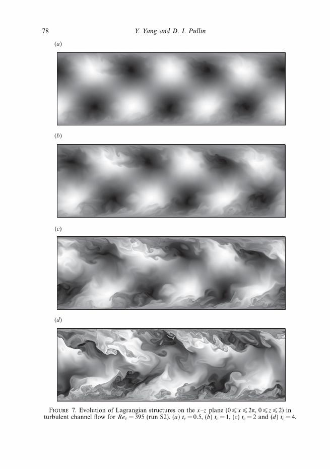
The temporal evolution of the Lagrangian field with colour intensity proportionalto φ ∈ [−1, 1] on the x–z plane in turbulent channel flow at Reτ = 395 is shown infigure 7. We can see that the initial regular, periodical blob-like objects are stretchedinto ramp-shaped structures by the mean shear and small-scale turbulent motions.Unlike the scalar properties for previous smoke visualization in turbulent boundarylayer experiments (e.g. Head & Bandyopadhyay 1981), the Lagrangian scalar field isnon-diffusive, so we can visualize and analyse fine structures with a high-resolutiongrid for φ. In figure 7 the vivid contrast evident between smooth and chaotic regionsillustrates the strong intermittency present in the Lagrangian field for the presentturbulent channel flow.

As shown in figure 1, we define the inclination angle α between an inclined structureprojected on the x–z plane and the x-direction. In terms of the variables in the multi-scale and multi-directional method as shown in figure 4, we have φ(x, y = yp, z)↔ϕ,x↔ x1, z↔ x2, α+↔〈�θ〉+ and α−↔〈�θ〉−. Evolution of individual components ofthe Lagrangian field can be obtained following the scale decomposition of φ on thex–z plane by (3.15). These are shown, at Reτ = 395, for the intermediate scale j =4and small scale j = 6 in figures 8 and 9, respectively. The characteristic length scalefor each scale index j is quantified in table 2. Then, the orientation information ofφ(x, t) on the x–z plane at different scales can be obtained by the normalized angularspectra Φj (�θ) defined in (3.18), which are shown in figure 10 at tc = 1 and tc = 4.The increasing Φj (�θ) at scales j � 3 shows a cascade process from large scales tosmall scales for φ in the temporal evolution. At each time, smaller scale structuresappear to show a greater tendency to ‘attach’ to the wall than larger structures in thesense of the predominance of small deviation angles in Φ(�θ) for large j .

As shown in figure 10, the angular spectra are almost symmetric for all scales.Therefore, assuming the symmetry of inclined structures with the centreline on the x–z plane in the statistical sense, we define the averaged inclination angle 〈α〉= (〈α+〉+〈α−〉)/2. Figure 11(a) shows the temporal evolution of 〈α〉 for Lagrangian structuresat intermediate and small scales (also refer figures 8 and 9). Here, the additional


(a)

(b)

(c)

(d)

Figure 7. Evolution of Lagrangian structures on the x–z plane (0 � x � 2π, 0 � z � 2) inturbulent channel flow for Reτ = 395 (run S2). (a) tc = 0.5, (b) tc = 1, (c) tc = 2 and (d) tc = 4.


(a) (b)

(c) (d)

Figure 8. Evolution of Lagrangian structures at scale 4 on the x–z plane (0 � x � 2π, 0 � z � 2)in turbulent channel flow for Reτ = 395 (run S2). (a) tc = 0.5, (b) tc = 1, (c) tc =2 and (d) tc = 4.

(a) (b)

(c) (d)

Figure 9. Evolution of Lagrangian structures at scale 6 on the x–z plane (0 � x � 2π, 0 � z � 2)in turbulent channel flow for Reτ = 395 (run S2). (a) tc = 0.5, (b) tc = 1, (c) tc =2 and (d) tc = 4.

averaging on 〈α〉 was taken over 50 x–z planes at y = yp uniformly distributedbetween y =0 and y = Ly . As shown in figure 9(a), the small-scale structures withsmall 〈α〉 appear at early times, around tc = 0.5, produced by intense near-wall shearmotions. Then, the small-scale structures are uplifted as shown in figures 9(c) and9(d ), which may signal ejections of low-speed fluid outward from the wall. Finally,some small-scale structures are bent downwards to the wall, which may be imprintsof the sweeps of high-speed fluid towards the wall. In figure 11(a), 〈α〉 grows withincreasing time; the trend is slightly slower for tc > 3. These observations are consistentwith the conceptual ejection-sweep-burst-inrush process (Hinze 1975). At tc =1 andtc = 4, 〈α〉 at different scales is shown in figure 11(a). We find that 〈α〉 of Lagrangianstructures at scales smaller than 20δν are higher for Reτ = 395 than for Reτ = 180,which may imply stronger turbulent transport in higher-Reynolds-number flows bycoherent motions that eject more fluid from the viscous sublayer to the logarithmicregion.

In addition, from simulations using different initial fields, e.g. φ0 = sin 3x andφ0 = πz (not shown), we find that the resulting Lagrangian structures producequantitatively similar averaged inclination angles at intermediate scales and smallscales for long times to those described above. This suggests that an attractor for


34567 x

z

10–10

10–8

10–6

10–4

10–2

100

Φj(

�θ)

(a)

–90 –45 0 45 90

�θ

�θ

10–10

10–8

10–6

10–4

10–2

100(b)

–90 –45 0 45 90

�θ

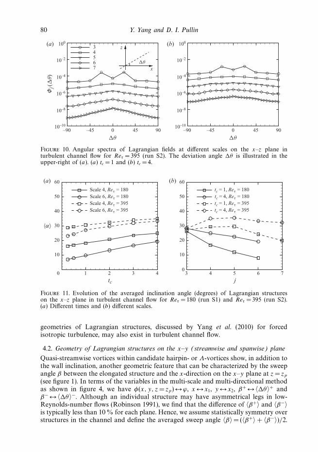
Figure 10. Angular spectra of Lagrangian fields at different scales on the x–z plane inturbulent channel flow for Reτ = 395 (run S2). The deviation angle �θ is illustrated in theupper-right of (a). (a) tc = 1 and (b) tc = 4.

1 2 3 40

10

20

30

40

50

60

Scale 4, Reτ = 180Scale 6, Reτ = 180Scale 4, Reτ = 395Scale 6, Reτ = 395

tc = 1, Reτ = 180tc = 4, Reτ = 180tc = 1, Reτ = 395tc = 4, Reτ = 395

tc

4 5 6 730

10

20

30

40

50

60

j

〈α〉

(a) (b)

Figure 11. Evolution of the averaged inclination angle (degrees) of Lagrangian structureson the x–z plane in turbulent channel flow for Reτ = 180 (run S1) and Reτ =395 (run S2).(a) Different times and (b) different scales.

geometries of Lagrangian structures, discussed by Yang et al. (2010) for forcedisotropic turbulence, may also exist in turbulent channel flow.

4.2. Geometry of Lagrangian structures on the x–y (streamwise and spanwise) plane

Quasi-streamwise vortices within candidate hairpin- or Λ-vortices show, in addition tothe wall inclination, another geometric feature that can be characterized by the sweepangle β between the elongated structure and the x-direction on the x–y plane at z = zp

(see figure 1). In terms of the variables in the multi-scale and multi-directional methodas shown in figure 4, we have φ(x, y, z = zp)↔ϕ, x↔ x1, y↔ x2, β+↔〈�θ〉+ andβ−↔〈�θ〉−. Although an individual structure may have asymmetrical legs in low-Reynolds-number flows (Robinson 1991), we find that the difference of 〈β+〉 and 〈β−〉is typically less than 10 % for each plane. Hence, we assume statistically symmetry overstructures in the channel and define the averaged sweep angle 〈β〉=(〈β+〉+ 〈β−〉)/2.


(a) (b)

(c) (d)

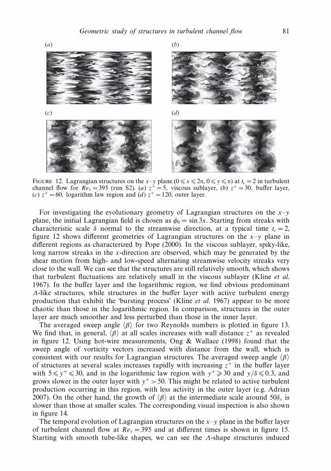
Figure 12. Lagrangian structures on the x–y plane (0 � x � 2π, 0 � y � π) at tc = 2 in turbulentchannel flow for Reτ = 395 (run S2). (a) z+ = 5, viscous sublayer, (b) z+ = 30, buffer layer,(c) z+ = 60, logarithm law region and (d) z+ = 120, outer layer.

For investigating the evolutionary geometry of Lagrangian structures on the x–y

plane, the initial Lagrangian field is chosen as φ0 = sin 3x. Starting from streaks withcharacteristic scale δ normal to the streamwise direction, at a typical time tc = 2,figure 12 shows different geometries of Lagrangian structures on the x–y plane indifferent regions as characterized by Pope (2000). In the viscous sublayer, spiky-like,long narrow streaks in the x-direction are observed, which may be generated by theshear motion from high- and low-speed alternating streamwise velocity streaks veryclose to the wall. We can see that the structures are still relatively smooth, which showsthat turbulent fluctuations are relatively small in the viscous sublayer (Kline et al.1967). In the buffer layer and the logarithmic region, we find obvious predominantΛ-like structures, while structures in the buffer layer with active turbulent energyproduction that exhibit the ‘bursting process’ (Kline et al. 1967) appear to be morechaotic than those in the logarithmic region. In comparison, structures in the outerlayer are much smoother and less perturbed than those in the inner layer.

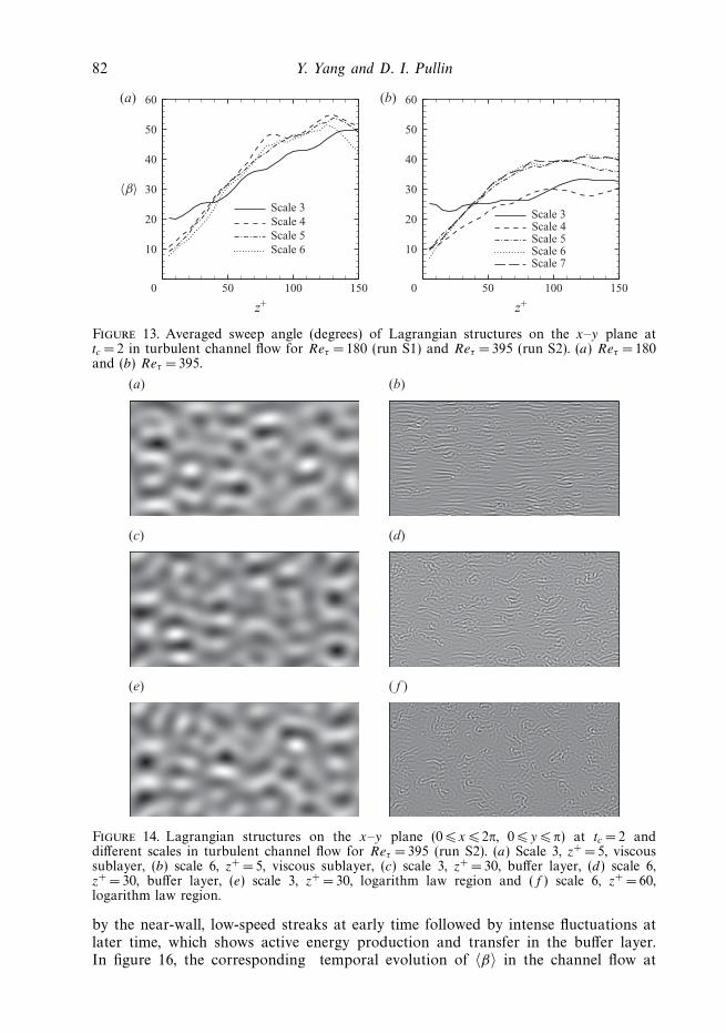
The averaged sweep angle 〈β〉 for two Reynolds numbers is plotted in figure 13.We find that, in general, 〈β〉 at all scales increases with wall distance z+ as revealedin figure 12. Using hot-wire measurements, Ong & Wallace (1998) found that thesweep angle of vorticity vectors increased with distance from the wall, which isconsistent with our results for Lagrangian structures. The averaged sweep angle 〈β〉of structures at several scales increases rapidly with increasing z+ in the buffer layerwith 5 � y+ � 30, and in the logarithmic law region with y+ � 30 and y/δ � 0.3, andgrows slower in the outer layer with y+ > 50. This might be related to active turbulentproduction occurring in this region, with less activity in the outer layer (e.g. Adrian2007). On the other hand, the growth of 〈β〉 at the intermediate scale around 50δν isslower than those at smaller scales. The corresponding visual inspection is also shownin figure 14.

The temporal evolution of Lagrangian structures on the x–y plane in the buffer layerof turbulent channel flow at Reτ = 395 and at different times is shown in figure 15.Starting with smooth tube-like shapes, we can see the Λ-shape structures induced


50 100 1500

10

20

30

40

50

60

z+

Scale 3Scale 4Scale 5Scale 6

Scale 3Scale 4Scale 5Scale 6Scale 7

〈β〉

(a)

50 100 1500

10

20

30

40

50

60

z+

(b)

Figure 13. Averaged sweep angle (degrees) of Lagrangian structures on the x–y plane attc = 2 in turbulent channel flow for Reτ =180 (run S1) and Reτ = 395 (run S2). (a) Reτ =180and (b) Reτ = 395.

(a) (b)

(c) (d)

(e) ( f )

Figure 14. Lagrangian structures on the x–y plane (0 � x � 2π, 0 � y � π) at tc = 2 anddifferent scales in turbulent channel flow for Reτ = 395 (run S2). (a) Scale 3, z+ = 5, viscoussublayer, (b) scale 6, z+ = 5, viscous sublayer, (c) scale 3, z+ = 30, buffer layer, (d) scale 6,z+ = 30, buffer layer, (e) scale 3, z+ = 30, logarithm law region and (f ) scale 6, z+ = 60,logarithm law region.

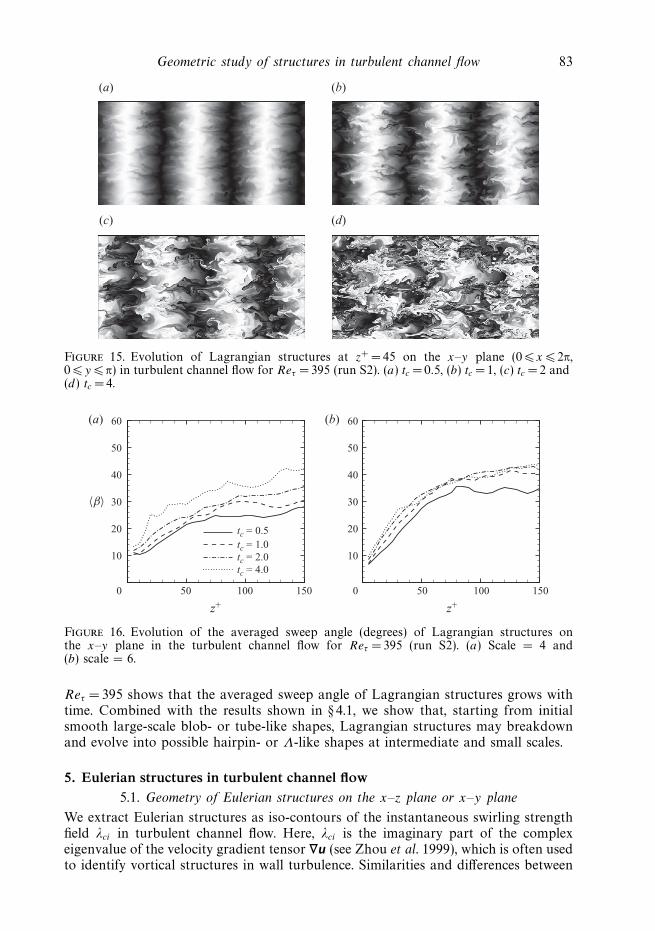
by the near-wall, low-speed streaks at early time followed by intense fluctuations atlater time, which shows active energy production and transfer in the buffer layer.In figure 16, the corresponding temporal evolution of 〈β〉 in the channel flow at


(a) (b)

(c) (d)

Figure 15. Evolution of Lagrangian structures at z+ = 45 on the x–y plane (0 � x � 2π,0 � y � π) in turbulent channel flow for Reτ = 395 (run S2). (a) tc = 0.5, (b) tc =1, (c) tc = 2 and(d) tc = 4.

tc = 0.5tc = 1.0tc = 2.0tc = 4.0

50 100 1500

10

20

30

40

50

60

z+

〈β〉

(a)

50 100 1500

10

20

30

40

50

60

z+

(b)

Figure 16. Evolution of the averaged sweep angle (degrees) of Lagrangian structures onthe x–y plane in the turbulent channel flow for Reτ = 395 (run S2). (a) Scale = 4 and(b) scale = 6.

Reτ = 395 shows that the averaged sweep angle of Lagrangian structures grows withtime. Combined with the results shown in § 4.1, we show that, starting from initialsmooth large-scale blob- or tube-like shapes, Lagrangian structures may breakdownand evolve into possible hairpin- or Λ-like shapes at intermediate and small scales.

5. Eulerian structures in turbulent channel flow5.1. Geometry of Eulerian structures on the x–z plane or x–y plane

We extract Eulerian structures as iso-contours of the instantaneous swirling strengthfield λci in turbulent channel flow. Here, λci is the imaginary part of the complexeigenvalue of the velocity gradient tensor ∇u (see Zhou et al. 1999), which is often usedto identify vortical structures in wall turbulence. Similarities and differences between


0 5

1 23

4 5 6

1015

2025

01z

0

0.5

1.0z

x

2

4y

3

2

1

0

y

6

x

(a)

(b)

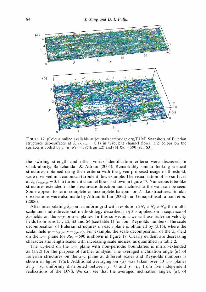
Figure 17. (Colour online available at journals.cambridge.org/FLM) Snapshots of Eulerianstructures (iso-surfaces at λci/λci,max =0.1) in turbulent channel flows. The colour on thesurfaces is coded by z. (a) Reτ = 395 (run L2) and (b) Reτ = 590 (run S3).

the swirling strength and other vortex identification criteria were discussed inChakraborty, Balachandar & Adrian (2005). Remarkably similar looking vorticalstructures, obtained using their criteria with the given proposed usage of threshold,were observed in a canonical turbulent flow example. The visualization of iso-surfacesat λci/λci,max = 0.1 in turbulent channel flows is shown in figure 17. Numerous tube-likestructures extended in the streamwise direction and inclined to the wall can be seen.Some appear to form complete or incomplete hairpin- or Λ-like structures. Similarobservations were also made by Adrian & Liu (2002) and Ganapathisubramani et al.(2006).

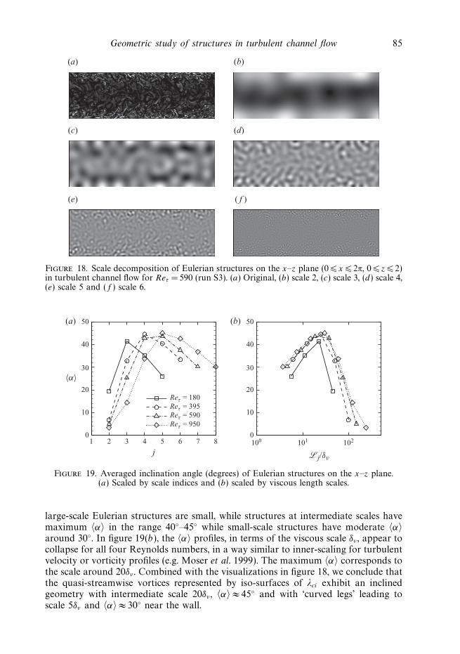
After interpolating λci on a uniform grid with resolution 2Nx ×Ny ×Nz, the multi-scale and multi-directional methodology described in § 3 is applied on a sequence ofλci-fields on the x–y or x–z planes. In this subsection, we will use Eulerian velocityfields from runs L1, L2, S3 and S4 (see table 1) for four Reynolds numbers. The scaledecomposition of Eulerian structures on each plane is obtained by (3.15), where thescalar field ϕ = λci(x, y = yp, z). For example, the scale decomposition of the λci-fieldon the x–z plane for Reτ = 590 is shown in figure 18. Clearly evident are decreasingcharacteristic length scales with increasing scale indices, as quantified in table 2.

The λci-field on the x–z plane with non-periodic boundaries is mirror-extendedas (3.22) for the purpose of further analysis. The averaged inclination angle 〈α〉 ofEulerian structures on the x–z plane at different scales and Reynolds numbers isshown in figure 19(a). Additional averaging on 〈α〉 was taken over 50 x–z planesat y = yp uniformly distributed between y = 0 and y = Ly from five independentrealizations of the DNS. We can see that the averaged inclination angles, 〈α〉, of


(a) (b)

(c) (d)

(e) ( f )

Figure 18. Scale decomposition of Eulerian structures on the x–z plane (0 � x � 2π, 0 � z � 2)in turbulent channel flow for Reτ = 590 (run S3). (a) Original, (b) scale 2, (c) scale 3, (d) scale 4,(e) scale 5 and (f ) scale 6.

1 2 3 4 5 6 7 8

Reτ = 180Reτ = 395Reτ = 590Reτ = 950

j101100 102

0

10

20

30

40

50

〈α〉

(a)

0

10

20

30

40

50(b)

Figure 19. Averaged inclination angle (degrees) of Eulerian structures on the x–z plane.(a) Scaled by scale indices and (b) scaled by viscous length scales.

large-scale Eulerian structures are small, while structures at intermediate scales havemaximum 〈α〉 in the range 40◦–45◦ while small-scale structures have moderate 〈α〉around 30◦. In figure 19(b), the 〈α〉 profiles, in terms of the viscous scale δν , appear tocollapse for all four Reynolds numbers, in a way similar to inner-scaling for turbulentvelocity or vorticity profiles (e.g. Moser et al. 1999). The maximum 〈α〉 corresponds tothe scale around 20δν . Combined with the visualizations in figure 18, we conclude thatthe quasi-streamwise vortices represented by iso-surfaces of λci exhibit an inclinedgeometry with intermediate scale 20δν , 〈α〉≈ 45◦ and with ‘curved legs’ leading toscale 5δν and 〈α〉≈ 30◦ near the wall.


50 100 1500

10

20

30

40

50

60

z+

〈β〉

(a)

50 100 1500

10

20

30

40

50

60

z+

(b)

Reτ = 180Reτ = 395Reτ = 590Reτ = 950

Figure 20. Averaged sweep angle (degrees) of Eulerian structures on the x–y plane atdifferent z+. (a) Scale 3 and (b) scale 5.

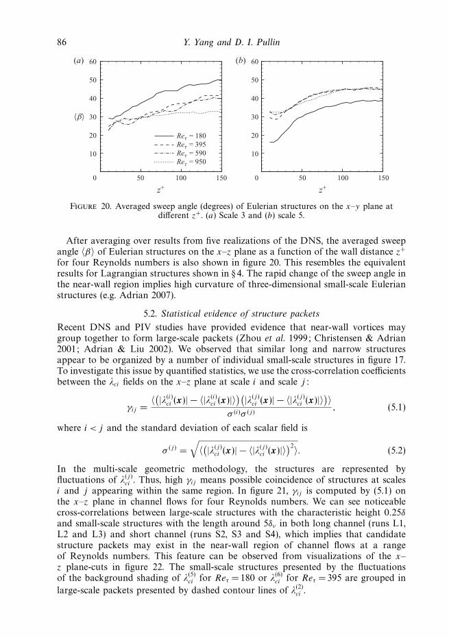
After averaging over results from five realizations of the DNS, the averaged sweepangle 〈β〉 of Eulerian structures on the x–z plane as a function of the wall distance z+

for four Reynolds numbers is also shown in figure 20. This resembles the equivalentresults for Lagrangian structures shown in § 4. The rapid change of the sweep angle inthe near-wall region implies high curvature of three-dimensional small-scale Eulerianstructures (e.g. Adrian 2007).

5.2. Statistical evidence of structure packets

Recent DNS and PIV studies have provided evidence that near-wall vortices maygroup together to form large-scale packets (Zhou et al. 1999; Christensen & Adrian2001; Adrian & Liu 2002). We observed that similar long and narrow structuresappear to be organized by a number of individual small-scale structures in figure 17.To investigate this issue by quantified statistics, we use the cross-correlation coefficientsbetween the λci fields on the x–z plane at scale i and scale j :

γij =〈(|λ(i)

ci (x)| − 〈|λ(i)ci (x)|〉

)(|λ(j )

ci (x)| − 〈|λ(j )ci (x)|〉

)〉

σ (i)σ (j ), (5.1)

where i < j and the standard deviation of each scalar field is

σ (j ) =

√〈(|λ(j )

ci (x)| − 〈|λ(j )ci (x)|〉

)2〉. (5.2)

In the multi-scale geometric methodology, the structures are represented byfluctuations of λ(j )

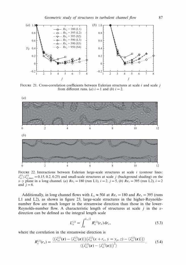
ci . Thus, high γij means possible coincidence of structures at scalesi and j appearing within the same region. In figure 21, γij is computed by (5.1) onthe x–z plane in channel flows for four Reynolds numbers. We can see noticeablecross-correlations between large-scale structures with the characteristic height 0.25δ

and small-scale structures with the length around 5δν in both long channel (runs L1,L2 and L3) and short channel (runs S2, S3 and S4), which implies that candidatestructure packets may exist in the near-wall region of channel flows at a rangeof Reynolds numbers. This feature can be observed from visualizations of the x–z plane-cuts in figure 22. The small-scale structures presented by the fluctuationsof the background shading of λ(5)

ci for Reτ = 180 or λ(6)ci for Reτ = 395 are grouped in

large-scale packets presented by dashed contour lines of λ(2)ci .


1 2 3 4 5 6 7 8–0.2 –0.2

0

0.2

0.4

0.6

0.8

1.0

γij

j

Reτ = 180 (L1)Reτ = 395 (L2)Reτ = 395 (S2)Reτ = 590 (L3)Reτ = 590 (S3)Reτ = 950 (S4)

1 2 3 4 5 6 7 8

0

0.2

0.4

0.6

0.8

1.0

j

(a) (b)

Figure 21. Cross-correlation coefficients between Eulerian structures at scale i and scale jfrom different runs. (a) i = 1 and (b) i =2.

0 2 4 6 8 10 12

0 2 4 6 8 10 12

(a)

(b)

Figure 22. Interactions between Eulerian large-scale structures at scale i (contour lines:

λ(i)ci /λ

(i)ci,max = 0.15, 0.2, 0.25) and small-scale structures at scale j (background shading) on the

x–y plane in a long channel. (a) Reτ =180 (run L1), i = 2, j =5, (b) Reτ = 395 (run L2), i = 2and j = 6.

Additionally, in long channel flows with Lx ≈ 50δ at Reτ = 180 and Reτ = 395 (runsL1 and L2), as shown in figure 23, large-scale structures in the higher-Reynolds-number flow are much longer in the streamwise direction than those in the lower-Reynolds-number flow. A characteristic length of structures at scale j in the x-direction can be defined as the integral length scale

L(j )x =

∫ Lx/2

0

R(j )x (rx) drx, (5.3)

where the correlation in the streamwise direction is

R(j )x (rx) =

〈(λ

(j )ci (x)− 〈λ(j )

ci (x)〉)(λ

(j )ci (x + rx, y = yp, z)− 〈λ(j )

ci (x)〉)〉

〈(λ

(j )ci (x)− 〈λ(j )

ci (x)〉)2〉

. (5.4)


0 10 20 30 40 50

0 10 20 30 40 50

(a)

(b)

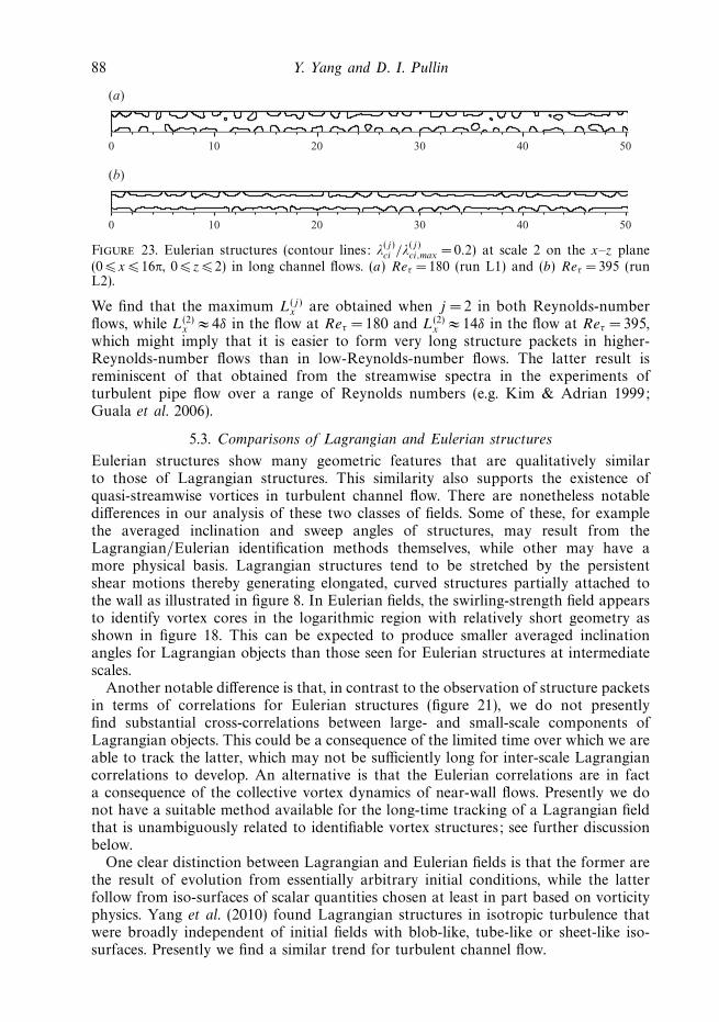
Figure 23. Eulerian structures (contour lines: λ(j )ci /λ

(j )ci,max =0.2) at scale 2 on the x–z plane

(0 � x � 16π, 0 � z � 2) in long channel flows. (a) Reτ = 180 (run L1) and (b) Reτ = 395 (runL2).

We find that the maximum L(j )x are obtained when j =2 in both Reynolds-number

flows, while L(2)x ≈ 4δ in the flow at Reτ = 180 and L(2)

x ≈ 14δ in the flow at Reτ = 395,which might imply that it is easier to form very long structure packets in higher-Reynolds-number flows than in low-Reynolds-number flows. The latter result isreminiscent of that obtained from the streamwise spectra in the experiments ofturbulent pipe flow over a range of Reynolds numbers (e.g. Kim & Adrian 1999;Guala et al. 2006).

5.3. Comparisons of Lagrangian and Eulerian structures

Eulerian structures show many geometric features that are qualitatively similarto those of Lagrangian structures. This similarity also supports the existence ofquasi-streamwise vortices in turbulent channel flow. There are nonetheless notabledifferences in our analysis of these two classes of fields. Some of these, for examplethe averaged inclination and sweep angles of structures, may result from theLagrangian/Eulerian identification methods themselves, while other may have amore physical basis. Lagrangian structures tend to be stretched by the persistentshear motions thereby generating elongated, curved structures partially attached tothe wall as illustrated in figure 8. In Eulerian fields, the swirling-strength field appearsto identify vortex cores in the logarithmic region with relatively short geometry asshown in figure 18. This can be expected to produce smaller averaged inclinationangles for Lagrangian objects than those seen for Eulerian structures at intermediatescales.

Another notable difference is that, in contrast to the observation of structure packetsin terms of correlations for Eulerian structures (figure 21), we do not presentlyfind substantial cross-correlations between large- and small-scale components ofLagrangian objects. This could be a consequence of the limited time over which we areable to track the latter, which may not be sufficiently long for inter-scale Lagrangiancorrelations to develop. An alternative is that the Eulerian correlations are in facta consequence of the collective vortex dynamics of near-wall flows. Presently we donot have a suitable method available for the long-time tracking of a Lagrangian fieldthat is unambiguously related to identifiable vortex structures; see further discussionbelow.

One clear distinction between Lagrangian and Eulerian fields is that the former arethe result of evolution from essentially arbitrary initial conditions, while the latterfollow from iso-surfaces of scalar quantities chosen at least in part based on vorticityphysics. Yang et al. (2010) found Lagrangian structures in isotropic turbulence thatwere broadly independent of initial fields with blob-like, tube-like or sheet-like iso-surfaces. Presently we find a similar trend for turbulent channel flow.


A connection between Lagrangian and Eulerian field geometries could perhaps beeduced by choice of initial conditions for the Lagrangian simulation that correspond toa physically interesting Eulerian field. In order to investigate Lagrangian mechanismsand vortex dynamics in idealized flows with Taylor–Green or Kida–Pelz initialconditions, Yang & Pullin (2010) introduced the vortex-surface field φ = φv satisfyingλω =0, where

λω =ω · ∇φ

|ω||∇φ| . (5.5)

In strictly inviscid flow, the Helmholtz vorticity theorems show that φ(x, t = 0)satisfying λω = 0 at t =0 will do so for t > 0. This fails for viscous flow. Further,for a given ω field, there are open existence and uniqueness questions concerning thedetermination of φ satisfying λω =0. A surrogate field may nevertheless be useful. Forthe present turbulent channel flows, we find that the choice φ = λci or φ = |ω| obtainedfrom the instantaneous Eulerian velocity field gives 〈|λω|〉 ≈ 0.5. While neither of theseis then close to a vortex-surface field, they may nevertheless provide interesting initialLagrangian fields. Hence, in addition to the initial Lagrangian fields described in§§ 4.1 and 4.2, we also performed simulations of Lagrangian structures evolving frominitial conditions defined by the three-dimensional filtered λci-field at scale 2. Thisproduced Lagrangian fields at a later time similar to those presented in §§ 4.1 and 4.2.

6. ConclusionsWe have developed a general multi-scale, multi-directional methodology based on

the mirror-extended curvelet transform to investigate the geometry of Lagrangian andEulerian structures, extracted respectively from a time sequence of the Lagrangianfields and from the instantaneous swirling-strength field in turbulent channel flow, forlow and moderate Reynolds numbers. This is used to quantify the statistical geometry,including the averaged inclination and sweep angles, of both classes of structures overa range of scales varying from the half-height of the channel to several viscous lengthscales. Quasi-streamwise Lagrangian and Eulerian vortical structures were detectedin the near-wall region and their geometries quantified. These comprise inclinedobjects, the averaged inclination angle of which is 35◦–45◦ principally within thelogarithmic region. The averaged sweep angle is 30◦–40◦ and the characteristic scaleis 20δν . ‘Curved legs’ are found in the viscous sublayer and buffer layer, for whichthe averaged inclination angle is 20◦–30◦, the averaged sweep angle is 15◦–30◦ and thescale is 5δν–10δν . The sweep angle of both structures increases rapidly in the bufferand logarithmic regions and grows mildly in the outer layer. The temporal evolutionof Lagrangian structures shows increasing inclination and sweep angles with time.The increasing magnitude in terms of both angles varies from 10◦ to 20◦ within thetypical ‘cyclic’ period from tc = 0.5 to tc = 4. This may quantify the lifting process ofquasi-streamwise vortices and the conceptional ejection-sweep-burst-inrush scenario.Both structures have slightly different geometries in flows for different Reynoldsnumbers. Although the averaged geometrical features of these objects are consistentwith the expected signatures of conceptual structures previously characterized ashairpin or Λ-vortices, we remark that the current methodology cannot distinguishbetween hairpin-like structures composed of two connected tubes and inclined tube-like structures that are not connected to each other via vortex lines.

Evidence for the existence of large-scale, Eulerian structure packets, comprisingcollections of individual small-scale geometrical objects, was obtained by finite


cross-correlations between large- and small-scale Eulerian structures. The large-scalepackets are located within the near-wall region with the typical height 0.25δ andmay extend over 10δ in the streamwise direction in moderate-Reynolds-number, longchannel flows.

The current methodology is based on a sequence of plane-cuts normal or parallel tothe streamwise direction in channel flows and so may also be suitable and convenientfor analysing experimental PIV data. The extension to fully three-dimensional datacould be achieved using the three-dimensional curvelet transform (Ying, Demanet &Candes 2005). The fast discrete curvelet transform algorithm with circular frequencywindow functions may be required for this. In addition, combined with the mirror-extension, the multi-scale geometric analysis (Bermejo-Moreno & Pullin 2008) usingthe fast three-dimensional curvelet transform can in principle be applied to detectcoherent structures in wall turbulence in order to study alternative non-local geometrysignatures based on principal curvatures. This could provide a means of testing anassumed structure in simplified models for wall turbulence (e.g. Perry & Chong 1982;Perry et al. 1986), structure-based subgrid models for the LES of near-wall channel(Chung & Pullin 2009) or boundary layer flows and the possible sparse representationof wall turbulence with the curvelet-based extraction method.

While the data analysed in this study are from low- to moderate-Reynolds-numberchannel flows, the present multi-scale and multi-directional methodology can easily beapplied to high-Reynolds-number data (e.g. Marusic et al. 2010) for turbulent channelor boundary layer flows to explore more geometric features such as the superstructuresin the outer layer (e.g. Hutchins & Marusic 2007) and the structural evolution in theturbulent transition (e.g. Wu & Moin 2009). Moreover, since high-Reynolds-numberwall turbulence exhibits scale separation, it would be interesting to investigate variousinter-scale interactions such as the large-scale modulation of small-scale motions andReynolds stresses using the curvelet multi-scale decomposition with quadrant analysis(e.g. Wallace, Brodkey & Eckelman 1972).

The authors are grateful to P. Koumoutsakos for providing generous access on theBrutus cluster at the ETH Zurich. The authors thank I. Bermejo-Moreno and D.Chung for helpful comments. This work has been supported in part by the NationalScience Foundation under grant DMS-1016111.

REFERENCES

Adrian, R. J. 2007 Hairpin vortex organization in wall turbulence. Phys. Fluids 19, 041301.

Adrian, R. J. & Liu, Z. C. 2002 Observation of vortex packets in direct numerical simulation offully turbulent channel flow. J. Vis. 5, 9–19.

del Alamo, J. C., Jimenez, J., Zandonade, P. & Moser, R. D. 2004 Scaling of the energy spectraof turbulent channels. J. Fluid Mech. 500, 135–144.

Bamberger, R. H. & Smith, M. J. T. 1992 A filter bank for the directional decomposition of images:theory and design. IEEE Trans. Signal Process. 40, 882–893.

Bandyopadhyay, P. 1980 Large structure with a characteristic upstream interface in turbulentboundary-layers. Phys. Fluids 23, 2326–2327.

Bermejo-Moreno, I. & Pullin, D. I. 2008 On the non-local geometry of turbulence. J. Fluid Mech.603, 101–135.

Candes, E., Demanet, L., Donoho, D. & Ying, L. 2006 Fast discrete curvelet transforms. MultiscaleModel. Simul. 5, 861–899.

Chakraborty, P., Balachandar, S. & Adrian, R. J. 2005 On the relationships between local vortexidentification schemes. J. Fluid Mech. 535, 189–214.


Chong, M. S., Perry, A. E. & Cantwell, B. J. 1990 A general classification of three-dimensionalflow fields. Phys. Fluids A 2, 765–777.

Christensen, K. T. & Adrian, R. J. 2001 Statistical evidence of hairpin vortex packets in wallturbulence. J. Fluid Mech. 431, 433–443.

Chung, D. & Pullin, D. I. 2009 Large-eddy simulation and wall modelling of turbulent channelflow. J. Fluid Mech. 631, 281–309.

Demanet, L. & Ying, L. 2007 Curvelets and wave atoms for mirror-extended images. In Proceedingsof the Society of Photo-optical Instrumentation Engineers (SPIE), vol. 6701, p. 67010J. SPIE.

Falco, R. E. 1977 Coherent motions in outer region of turbulent boundary-layers. Phys. Fluids 20,S124–S132.

Ganapathisubramani, B., Longmire, E. K. & Marusic, I. 2006 Experimental investigation ofvortex properties in a turbulent boundary layer. Phys. Fluids 18, 055105.

Green, M. A., Rowley, C. W. & Haller, G. 2007 Detection of Lagrangian coherent structures inthree-dimensional turbulence. J. Fluid Mech. 572, 111–120.

Guala, M., Hommema, S. E. & Adrian, R. J. 2006 Large-scale and very-large-scale motions inturbulent pipe flow. J. Fluid Mech. 554, 521–542.

Haller, G. 2001 Distinguished material surfaces and coherent structures in three-dimensional fluidflows. Physica D 149, 248–277.

Head, M. R. & Bandyopadhyay, P. 1981 New aspects of turbulent boundary-layer structure.J. Fluid Mech. 107, 297–338.

Hinze, J. O. 1975 Turbulence, 2nd edn. McGrow-Hill.

Honkan, A. & Andreopoulos, Y. 1997 Vorticity, strain-rate and dissipation characteristics in thenear-wall region of turbulent boundary layers. J. Fluid Mech. 350, 29–96.

Hunt, J. C. R., Wray, A. A. & Moin, P. 1988 Eddies, stream, and convergence zones in turbulentflows. Center for Turbulence Research Report CTR-S88 , pp. 193–208.

Hutchins, N. & Marusic, I. 2007 Evidence of very long meandering features in the logarithmicregion of turbulent boundary layers. J. Fluid Mech. 579, 1–28.

Jeong, J. & Hussain, F. 1995 On the identification of a vortex. J. Fluid Mech. 285, 69–94.

Jimenez, J., del Alamo, J. C. & Flores, O. 2004 The large-scale dynamics of near-wall turbulence.J. Fluid Mech. 505, 179–199.

Kim, J., Moin, P. & Moser, R. 1987 Turbulence statistics in fully-developed channel flow at lowReynolds-number. J. Fluid Mech. 177, 133–166.

Kim, K. C. & Adrian, R. J. 1999 Very large-scale motion in the outer layer. Phys. Fluids 11,417–422.

Kline, S. J., Reynolds, W. C., Schraub, F. A. & Runstadl, P. W. 1967 Structure of turbulentboundary layers. J. Fluid Mech. 30, 741–773.

Liu, Z. C., Landreth, C. C., Adrian, R. J. & Hanratty, T. J. 1991 High-resolution measurementof turbulent structure in a channel with particle image velocimetry. Exp. Fluids 10, 301–312.

Ma, J., Hussaini, M. Y., Vasilyev, O. V. & Le Dimet, F.-X. 2009 Multiscale geometric analysis ofturbulence by curvelets. Phys. Fluids 21, 075104.

Marusic, I. 2001 On the role of large-scale structures in wall turbulence. Phys. Fluids 13, 735–743.

Marusic, I., McKeon, B. J., Monkewitz, P. A., Nagib, H. M., Smits, A. J. & Sreenivasan, K. R.

2010 Wall-bounded turbulent flows at high Reynolds numbers: recent advances and keyissues. Phys. Fluids 22, 065103.

Moin, P. & Kim, J. 1982 Numerical investigation of turbulent channel flow. J. Fluid Mech. 118,341–377.

Moin, P. & Kim, J. 1985 The structure of the vorticity field in turbulent channel flow. Part 1.Analysis of instantaneous fields and statistical correlations. J. Fluid Mech. 155, 441–464.

Moser, R. D., Kim, J. & Mansour, N. N. 1999 Direct numerical simulation of turbulent channelflow up to Reτ = 590. Phys. Fluids 11, 943–945.

Okamoto, N., Yoshimatsu, K., Schneider, K., Farge, M. & Kaneda, Y. 2007 Coherent vortices inhigh resolution direct numerical simulation of homogeneous isotropic turbulence: a waveletviewpoint. Phys. Fluids 19, 115109.

Ong, L. & Wallace, J. M. 1998 Joint probability density analysis of the structure and dynamics ofthe vorticity field of a turbulent boundary layer. J. Fluid Mech. 367, 291–328.


Panton, R. L. 2001 Overview of the self-sustaining mechanisms of wall turbulence. Prog. Aerosp.Sci. 37, 341–383.

Perry, A. E. & Chong, M. S. 1982 On the mechanism of wall turbulence. J. Fluid Mech. 119,173–217.

Perry, A. E., Henbest, S. & Chong, M. S. 1986 A theoretical and experimental-study of wallturbulence. J. Fluid Mech. 165, 163–199.

Perry, A. E. & Marusic, I. 1995 A wall-wake model for the turbulence structure of boundary-layers.Part 1. Extension of the attached eddy hypothesis. J. Fluid Mech. 298, 361–388.

Pope, S. B. 2000 Turbulent Flows . Cambridge University Press.

Pullin, D. I. 1981 The non-linear behavior of a constant vorticity layer at a wall. J. Fluid Mech.108, 401–421.

Robinson, S. K. 1991 Coherent motions in the turbulent boundary layer. Annu. Rev. Fluid Mech.23, 601–639.

Spalart, R. R., Moser, R. D. & Rogers, M. M. 1991 Spectral methods for the Navier–Stokesequations with one infinite and two periodic directions. J. Comput. Phys. 96, 297–324.

Theodorsen, T. 1952 Mechanism of turbulence. In Proceedings of the Second Midwestern Conferenceon Fluid Mechanics, Ohio State University, Columbus, 17–19 March , pp. 1–18.

Townsend, A. A. 1976 The Structure of Turbulent Shear Flow , 2nd edn. Cambridge UniversityPress.

Wallace, J. M., Brodkey, R. S. & Eckelman, H. 1972 Wall region in turbulent shear flow. J. FluidMech. 54, 39–48.

Wu, X. & Moin, P. 2009 Direct numerical simulation of turbulence in a nominally zero-pressure-gradient flat-plate boundary layer. J. Fluid Mech. 630, 5–41.

Yang, Y. & Pullin, D. I. 2010 On Lagrangian and vortex-surface fields for flows with Taylor–Greenand Kida–Pelz initial conditions. J. Fluid Mech. 661, 446–481.

Yang, Y., Pullin, D. I. & Bermejo-Moreno, I. 2010 Multi-scale geometric analysis of Lagrangianstructures in isotropic turbulence. J. Fluid Mech. 654, 233–270.

Ying, L., Demanet, L. & Candes, E. 2005 3D discrete curvelet transform. In Proceedings of theSociety of Photo-optical Instrumentation Engineers (SPIE), vol. 5914, pp. 351–361. SPIE.

Zhou, J., Adrian, R. J., Balachandar, S. & Kendall, T. M. 1999 Mechanisms for generatingcoherent packets of hairpin vortices in channel flow. J. Fluid Mech. 387, 353–396.

geometric study of lagrangian and eulerian structures in ...geometric study of lagrangian and...

Documents