aerodynamic and structural design and analysis of …
TRANSCRIPT

AERODYNAMIC AND STRUCTURAL DESIGN AND ANALYSIS OF AN ELECTRIC POWERED MINI UAV
A THESIS SUBMITTED TO THE GRADUATE SCHOOL OF NATURAL AND APPLIED SCIENCES
OF MIDDLE EAST TECHNICAL UNIVERSITY
BY
ALPAY DEMİRCAN
IN PARTIAL FULFILLMENT OF THE REQUIREMENTS FOR
THE DEGREE OF MASTER OF SCIENCE IN
AEROSPACE ENGINEERING
MAY 2016


Approval of the thesis:
AERODYNAMIC AND STRUCTURAL DESIGN
AND ANALYSIS OF AN ELECTRIC POWERED MINI UAV
submitted by ALPAY DEMİRCAN in partial fulfillment of the requirements for the degree of Master of Science in Aerospace Engineering Department, Middle East Technical University by,
Prof. Dr. Gülbin Dural Ünver Dean, Graduate School of Natural and Applied Sciences
___________________
Prof. Dr. Ozan Tekinalp Head of Department, Aerospace Engineering
___________________
Prof. Dr. Altan Kayran Supervisor, Aerospace Engineering Dept., METU
___________________
Examining Committee Members:
Prof. Dr. Serkan Özgen Aerospace Engineering Dept., METU
___________________
Prof. Dr. Altan Kayran Aerospace Engineering Dept., METU
___________________
Prof. Dr. Nafiz Alemdaroğlu School of Civil Aviation, Atılım University
___________________
Asst. Prof. Dr. Ercan Gürses Aerospace Engineering Dept., METU
___________________
Asst. Prof. Dr. Harika S. Kahveci Aerospace Engineering Dept., METU
___________________
Date:
___________________

iv
I hereby declare that all information in this document has been obtained and
presented in accordance with academic rules and ethical conduct. I also declare
that, as required by these rules and conduct, I have fully cited and referenced
all material and results that are not original to this work.
Name, Last Name : Alpay DEMİRCAN
Signature :

v
ABSTRACT
AERODYNAMIC AND STRUCTURAL DESIGN
AND ANALYSIS OF AN ELECTRIC POWERED MINI UAV
Demircan, Alpay
M. S., Department of Aerospace Engineering
Supervisor: Prof. Dr. Altan Kayran
May 2016, 173 pages
The aim of this study is to describe the aerodynamic and structural design of an
electric powered portable Mini UAV. Conceptual design, structural design and
analysis of the wing and detail design phases of the UAV are presented in the study.
Fixed wing mini UAV configuration with fixed – pitch propeller has been chosen for
the design. In order to provide multi-mission capability, payload of the UAV is
designed as a replaceable mission compartment. System requirements and mission
profiles of the airplane are adopted from competitor analysis and critical design
parameters are defined to perform flight performance calculations in the conceptual
design phase. A dynamic thrust estimation model is proposed for the electric motor
and fixed – pitch propeller propulsion system. Endurance and range calculations for a
battery powered aircraft are also described in the study.
Components of the aircraft structure are designed using composite materials. In order
to decide structural layout of the wing, CFD analysis of the wing is performed for
limit load condition and aerodynamic loading is determined. Structural analysis of
the wing is performed for two different structural layouts by using the aerodynamic
load determined in CFD analysis. I spar and tubular spar configurations are

vi
considered for the wing structure and comparison of stress loads on the structural
components of the wing for these two different design configurations is presented.
Overall structural layout, portability and ease of transportation requirements are
considered in the detailed structural design phase. Manufacturing and assembly
issues are also taken into account and at the end of this study, ready to manufacture
design is presented.
Keywords: Mini UAV, electric powered UAV, fixed pitch propeller, airplane design,
finite element analysis, composite structure, structural design

vii
ÖZ
ELEKTRİKLİ BİR MİNİ İHA’NIN
AERODİNAMİK VE YAPISAL TASARIMI VE ANALİZİ
Demircan, Alpay
Yüksek Lisans, Havacılık ve Uzay Mühendisliği Bölümü
Tez Yöneticisi: Prof. Dr. Altan Kayran
Mayıs 2016, 173 sayfa
Bu çalışmanın amacı elektrikli bir portatif Mini İHA'nın aerodinamik ve yapısal
tasarımını belirlemektir. Çalışma kapsamında kavramsal tasarım, kanadın yapısal
tasarımı ile analizi ve detay tasarım süreçleri gösterilmiştir.
Tasarımda sabit hatveli pervanenin kullanıldığı sabit kanatlı bir Mini İHA
konfigürasyonu seçilmiştir. Çoklu görevlere uygunluğun sağlanması için faydalı yük
olarak değiştirilebilir bir görev bölmesi seçilmiştir. Sistem gereksinimleri ve görev
profilleri rakip analizleriyle belirlenmiş ve konsept tasarım sürecinde uçuş
performansı hesaplamalarında kullanılmıştır. Çalışmada sabit hatveli pervane
kullanan elektrikli uçaklar için dinamik itki hesaplama modeli sunulmuş, pilli uçaklar
için uçuş süresi ve menzil hesaplamaları gösterilmiştir.
Uçağın yapısal bileşenleri kompozit malzeme kullanarak tasarlanmıştır. Kanadın
yapısal tasarımının belirlenmek için limit yük koşulları altındaki aerodinamik
yükleme HAD analizi yapılarak belirlenmiştir. Kanadın yapısal analizi iki farklı
yapısal tasarım için HAD analiziyle elde edilmiş olan aerodinamik yükler
kullanılarak yapılmıştır. Kanadın yapısal konfigürasyonlarında I tipi kanat kirişi ve

viii
boru kiriş kullanılmış ve bu iki farklı kanat yapısalı konfigürasyonu için gerilme
yüklerinin kıyaslanması gösterilmiştir.
Detay tasarım sürecinde genel yapısal tasarım, portatiflik ve kolay taşınabilirlik
gereksinimleri dikkate alınmıştır. Üretim ve birleştirme hususlarının da dikkate
alındığı bu çalışmanın sonunda üretime hazır bir tasarım gerçekleştirilmiştir.
Anahtar Kelimeler: mini İHA, elektrikli mini İHA, sabit hatveli pervane, uçak
tasarımı, sonlu elemanlar analizi, kompozit yapı, yapısal tasarım

ix
to my grandfather…

x
ACKNOWLEDGEMENTS
I would like to thank my supervisor Prof. Dr. Altan KAYRAN for his guidance,
advices, encouragements and supports throughout this study. Almost all applied
engineering skills I gained are because of his “abundant projects and homeworks”
and I will always proud to say that “I have studied on it when I was taking Prof.
Kayran’s course”.
I would like to express my sincere gratitude to Prof. Dr. Nafiz ALEMDAROĞLU for
his invitation to METU TUAV and Mini UAV projects. His guidance and helps
during this period and encouraging me to design and manufacture my very first UAV
prototype “Saka Mini UAV" is the most important milestone of my engineering life.
Fundamentals of this thesis work are also based on my experiences gained during
this period. I would like to express my further gratitude to my supervisor Prof. Dr.
Altan KAYRAN to share his profound knowledge on composite structures design
and workshop.
I would also like to thank all of Anatolian Craft 2011 team members one by one and
I would like to give my special appreciations to Mehmet Harun ÖZKANAKTI, who
is also my METU Rugby team mate, played shoulder to shoulder with me against
opponents in the rugby field, for his continuous friendship and support throughout
my entire study.
I would like to give my special thanks to research assistants of the METU Aerospace
Engineering Department for their moral support throughout my study and special
appreciations to Derya KAYA for her supports during my experiments.
I would also like to thank Ali İhsan GÖLCÜK for his moral support who is also my
“Kabzadaş” in archery.
Finally, I would like to thank my family, supported me and love at all conditions
throughout my life and thanks for their patience.

xi
TABLE OF CONTENTS
ABSTRACT .............................................................................................................v
ÖZ ......................................................................................................................... vii
ACKNOWLEDGEMENTS ......................................................................................x
TABLE OF CONTENTS ........................................................................................ xi
LIST OF TABLES .................................................................................................xiv
LIST OF FIGURES ............................................................................................. xvii
LIST OF SYMBOLS ........................................................................................... xxii
LIST OF ABBREVIATIONS ............................................................................. xxiii
CHAPTERS............................................................................................................ iv
1. INTRODUCTION..........................................................................................1
1.1. Unmanned Aerial Vehicles..........................................................................1
1.2. History of Unmanned Aerial Vehicles .........................................................2
1.3. Mini UAVs .................................................................................................4
1.4. Demircan Mini UAV...................................................................................6
2. CONCEPTUAL DESIGN ............................................................................11
2.1. Introduction .............................................................................................. 11
2.2. Regulations ............................................................................................... 11
2.3. Design Requirements ................................................................................ 12
2.4. Configuration Layout ................................................................................ 17
2.5. Airfoil Selection and Wing Sizing ............................................................. 19
2.6. Preliminary Wing Analysis ....................................................................... 32
2.7. Sizing ........................................................................................................ 39

xii
2.8. Fundamental Design Parameters ............................................................... 45
2.9. Constraint Analysis (W/S vs. PA/W) ......................................................... 57
2.10. Dynamic Thrust Estimation .................................................................... 61
2.11. Constraint Analysis (W/S vs P/W) .......................................................... 79
2.12. Aircraft Performance Analysis ................................................................ 80
2.13. V-n Diagram ........................................................................................... 95
2.14. Preliminary Performance Analysis ........................................................ 102
2.15. Longitudinal Stability and CG Location ................................................ 108
2.16. System Components and Weight Distribution ....................................... 111
2.17. Final Conceptual Design ....................................................................... 114
3. NUMERICAL ANALYSIS OF THE WING .............................................. 117
3.1. Introduction ............................................................................................ 117
3.2. CFD Analysis of the Wing at Limit Load ................................................ 117
3.3. Wing Structure Design ............................................................................ 126
3.4. Material Definitions ................................................................................ 127
3.5. Structural Analysis of Wing .................................................................... 129
4. DETAIL DESIGN ..................................................................................... 139
4.1. Introduction ............................................................................................ 139
4.2. Composite UAV Manufacturing Study ................................................... 140
4.3. Detail Design .......................................................................................... 142
4.4. System Components ............................................................................... 151
4.5. Weight Check and CG Location ............................................................. 152
4.6. End of the Detail Design ......................................................................... 154
5. CONCLUSION ......................................................................................... 155
5.1. Future Work ........................................................................................... 156

xiii
REFERENCES ..................................................................................................... 157
APPENDICES ...................................................................................................... 160
APPENDIX A: COMPETITOR MINI UAVS ................................................... 161
APPENDIX B: COMPONENT DRAG BUILDUP ............................................ 163
APPENDIX C: AERODYNAMIC RELATIONS ASSOCIATED WITH LIFT
DRAG AND FLIGHT VELOCITY ................................................................... 165
APPENDIX D: CONSTRAINT EQUATIONS .................................................. 169
D.1. Climb Speed Constraint .......................................................................... 169
D.2. Maximum Rate of Climb Constraint ....................................................... 169
D.3. Maximum Speed Constraint ................................................................... 170
D.4. Sustained Level Turn Constraint ............................................................ 171
APPENDIX E: APC – SLOW FLYER – 11X4.7 PROPELLER ........................ 173

xiv
LIST OF TABLES
TABLES
Table 1.1. NATO UAS Classification Guide [3] ....................................................... 2
Table 1.2. Primary Design Requirements of Demircan Mini UAV ............................ 7
Table 2.1. SHT-İHA Constraints............................................................................. 12
Table 2.2. General Design Requirements of Demircan Mini UAV .......................... 13
Table 2.3. Layout Classification for Mini UAVs ..................................................... 15
Table 2.4. Layout Classification of Competitor Mini UAVs.................................... 15
Table 2.5. Average Design Parameters of Competitor Mini UAVs.......................... 15
Table 2.6. UAV Vision CM100 Specifications [14] ................................................ 16
Table 2.7. Initial Design Parameters of Demircan Mini UAV ................................. 17
Table 2.8. Standard Atmosphere Table (AMSL) ..................................................... 20
Table 2.9. Lift Coefficient Requirements at Different Speeds and Altitude ............. 20
Table 2.10. Reynolds Number Range ...................................................................... 21
Table 2.11. Aerodynamic Coefficients of the MH114 Airfoil. ................................ 26
Table 2.12. Wing Parameters .................................................................................. 31
Table 2.13. Aerodynamic Coefficients of the Multi-Tapered Wing ......................... 33
Table 2.14. Lift Coefficient Table ........................................................................... 37
Table 2.15. Initial Sizing Parameters of Demircan Mini UAV ................................ 39
Table 2.16. Horizontal Tail Dimensions.................................................................. 41
Table 2.17. Vertical Tail Dimensions (Double Fin) ................................................ 42
Table 2.18. Fuselage Dimensions ........................................................................... 43
Table 2.19. Boom Dimensions ................................................................................ 44
Table 2.20. Wetted Areas ....................................................................................... 45
Table 2.21. Interference Factors, Q ......................................................................... 46
Table 2.22. Parasite Drag Coefficient Components ................................................. 47
Table 2.23. (L/D)max Velocities with Altitude ....................................................... 53
Table 2.24. (CL3/2/CD)max Velocities at Different Altitudes .................................... 54
Table 2.25. Comparison of (L/D)max and (CL3/2/CD)max Results ................................ 54
Table 2.26. Comp. of (L/D)max and (CL3/2/CD)max Velocities at Different Altitudes . 54

xv
Table 2.27. Summary of Fundamental Design Parameters ....................................... 56
Table 2.28. Constraint Analysis Requirements ........................................................ 57
Table 2.29. EMAX-GT2218/11 Performance with Recommended Propellers [22] .. 63
Table 2.30. Experimental Setup Components .......................................................... 64
Table 2.31. Experimental and Calculated Results .................................................... 66
Table 2.32. APC-SF-11x4.7, Experimental Performance Data [21] ......................... 69
Table 2.33. Corrected Shaft Power Calculations ...................................................... 71
Table 2.34. Theoretical and Actual V(R/C)max Variation with Altitude ....................... 83
Table 2.35. Climb Angles with Altitude .................................................................. 84
Table 2.36. Time to Climb Table............................................................................. 86
Table 2.37. Minimum Glide Angles ........................................................................ 86
Table 2.38. Glide velocities, Minimum Glide Angles and Descent Rates ................. 87
Table 2.39. Takeoff Distances for Various Altitudes ............................................... 88
Table 2.40. Max. Endurance and Corresponding Velocities at Various Altitudes ..... 92
Table 2.41. Max. Ranges and Corresponding Velocities at Different Altitudes ........ 93
Table 2.42. Critical Design Speeds .......................................................................... 93
Table 2.43. Mission Profile and Required Battery Capacity..................................... 94
Table 2.44. Total Battery Capacity Requirement at Design Altitudes ...................... 94
Table 2.45. nmax, Bank Angles, Turn Radii for Various Altitudes ............................ 98
Table 2.46. Load Factor and Corresponding Velocities at Sea Level ..................... 101
Table 2.47. XFLR5 – VLM Analysis Results for Stall and Cruise Conditions ....... 104
Table 2.48. Table of XFLR5 – VLM Analysis Results at 1000 m .......................... 107
Table 2.49. Aircraft Components .......................................................................... 112
Table 2.50. Aircraft System Components and CG Locations ................................. 113
Table 2.51. Summary of General Design Features ................................................. 116
Table 3.1. Limit Load Condition Parameters ......................................................... 117
Table 3.2. Wall Distance Estimation Parameters for Wing Analysis ...................... 120
Table 3.3. Mesh Statistics ..................................................................................... 122
Table 3.4. Mesh Quality wrt. Skewness Value [31] ............................................... 122
Table 3.5. Limit Load Analysis Results for 𝛼 = 3.8° ............................................ 124
Table 3.6. Material Definitions ............................................................................. 128
Table 3.7. Material Properties to be used in Finite Element Analysis [38] ............. 128

xvi
Table 3.8. Element Types and Number of Elements of Structural Models ............. 130
Table 3.9. Global Maximum Stress and Deflections .............................................. 134
Table 4.1. General Sizing of HUAVN [41], [42] ................................................... 140
Table 4.2. E-Glass/Balsa Material Densities ......................................................... 141
Table 4.3. Comparison of Conceptual and Detail Design Weights ........................ 152
Table 4.4. Aircraft System Components and CG Locations of Detail Design ........ 153

xvii
LIST OF FIGURES
FIGURES
Figure 1.1. Sperry “Flying Bomb” [5] .......................................................................2
Figure 1.2. Kettering Bug [6] ....................................................................................3
Figure 1.3. IAI - RQ-2 Pioneer [8] ............................................................................4
Figure 1.4. ISR Mission Performed by a Single Operator [10] ...................................5
Figure 1.5. Civilian Market for UAS in Europe by Category 2008-2017 [11] ............5
Figure 1.6. Design Flowchart .................................................................................. 10
Figure 2.1. Mission Profile ...................................................................................... 13
Figure 2.2. UAV Vision CM100 Gimbal [14] ......................................................... 16
Figure 2.3. Design Configuration of Demircan Mini UAV ...................................... 19
Figure 2.4. Maximum Lift Coefficients for Different Stall Velocities ...................... 21
Figure 2.5. Cl vs. Alpha Curves of Candidate Airfoils at Re=230000 ...................... 22
Figure 2.6. Cl/Cd vs. Alpha Curves of Candidate Airfoils at Re=230000 ................. 23
Figure 2.7. MH114 Airfoil ...................................................................................... 24
Figure 2.8. Cl vs. Alpha Curve of MH114 at Re=230000 ........................................ 24
Figure 2.9. Cl/Cd vs. Alpha Curve of MH114 at Re=230000 ................................... 25
Figure 2.10. Cm,c/4 vs. Alpha Curve of MH114 at Re=230000 ................................. 25
Figure 2.11. Effect of Taper Ratio on Flow Sep. at Near-Stall Conditions [15] ........ 27
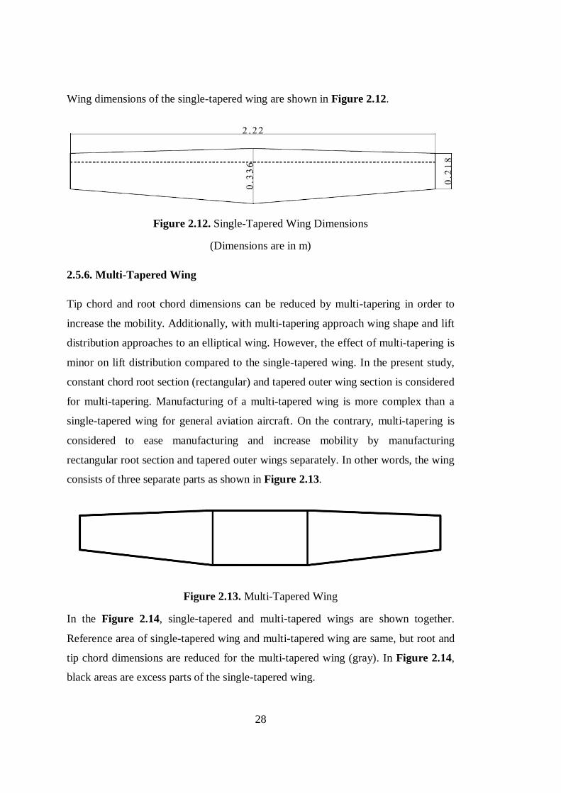
Figure 2.12. Single-Tapered Wing Dimensions ....................................................... 28
Figure 2.13. Multi-Tapered Wing ............................................................................ 28
Figure 2.14. Chord Reduction and Dimensions of the Multi-Tapered Wing ............. 29
Figure 2.15. Multi-Tapered Wing Dimensions ........................................................ 31
Figure 2.16. Wing Elements (3240 Panel Elements – 1600 VLM Elements) ........... 32
Figure 2.17. CL vs Alpha Results for 2D airfoil and 3D Wing Analyses. ................. 33
Figure 2.18. CL/CD Curves of Finite Wing Analysis Results. ................................... 34
Figure 2.19. Cmc/4 vs Alpha Results of Wing Analysis Results ............................... 34
Figure 2.20. Cp Distribution on the Upper and Lower Surfaces at 𝛼 = 0°. .............. 35
Figure 2.21. Cp Distribution on Wing at 𝛼 = 0° (Isometric View) .......................... 35
Figure 2.22. Flapped and Unlapped Wing Conditions ............................................. 36

xviii
Figure 2.23. CL vs. Alpha Results for LLT Analysis ............................................... 37
Figure 2.24. CL/CD vs. Alpha Results for LLT Analysis .......................................... 38
Figure 2.25. Drag Polar of the Wing ....................................................................... 38
Figure 2.26. Horizontal Tail Dimensions (m) .......................................................... 41
Figure 2.27. Vertical Tail Dimensions (m) .............................................................. 42
Figure 2.28. Fuselage Dimensions (m) .................................................................... 43
Figure 2.29. Boom Dimensions (m) ........................................................................ 44
Figure 2.30. Conceptual Configuration Layout ....................................................... 44
Figure 2.31. Parasite Drag Contributions ................................................................ 48
Figure 2.32. Induced Drag Factor, 𝛿 for different AR and 𝜆 [15] ............................. 48
Figure 2.33. Drag Polar .......................................................................................... 51
Figure 2.34. Variation of Cruise and Loitering Velocities with Altitude .................. 55
Figure 2.35. Variations of CL/CD and CL3/2
/CD relations vs. Velocity at 1000 m ...... 56
Figure 2.36. Constraint Diagram for PA/W .............................................................. 60
Figure 2.37. Propeller Efficiency vs. Advance Ratio for Various Pitch Angles [20] 61
Figure 2.38. EMAX – GT2218/11 Brushless Out-Runner Motor ............................ 62
Figure 2.39. APC Slow Flyer 11x4.7 Propeller and 𝜂𝑝𝑟 vs. J plot ........................... 63
Figure 2.40. METU Aerospace Engineering Dept. Low Speed Wind Tunnel .......... 64
Figure 2.41. Experimental Setup ............................................................................. 65
Figure 2.42. Experimental Setup Placed in the Wind Tunnel ................................... 65
Figure 2.43. Dynamic Thrust and Power Available vs. Velocity ............................. 66
Figure 2.44. Propeller Efficiency vs. Velocity......................................................... 67
Figure 2.45. Propeller RPM vs. Velocity ................................................................ 67
Figure 2.46. Shaft Power vs. Velocity ..................................................................... 67
Figure 2.47. Draining Current vs. Velocity ............................................................. 68
Figure 2.48. Constant and Corrected Shaft Power vs. Velocity ............................... 71
Figure 2.49. Effect of Power Correction Factor on Shaft Power .............................. 72
Figure 2.50. Dynamic Thrust Estimation Model ..................................................... 73
Figure 2.51. Effects of AF and PcF parameters on Dynamic Thrust Curve .............. 74
Figure 2.52. Dynamic Thrust Model and Experimental Thrust Results .................... 75
Figure 2.53. Power Available Curves of Experimental and Dynamic Thrust Model 75
Figure 2.54. Dynamic Thrust at Various Altitudes .................................................. 76

xix
Figure 2.55. Rotational Speed of the Propeller vs. Velocity at Various Altitudes ..... 77
Figure 2.56. Power Available vs. Velocity for Various Altitudes ............................. 78
Figure 2.57. Propeller Efficiency vs. Velocity for Various Altitudes ....................... 78
Figure 2.58. Constraint Diagram for P/W ................................................................ 79
Figure 2.59. Drag (TR) and Thrust Available Curves ............................................... 81
Figure 2.60. Power Required and Power Available Curves ...................................... 81
Figure 2.61. (PR)min and (R/C)max Velocities ............................................................ 82
Figure 2.62. Rate of Climb Variation with Altitude ................................................. 83
Figure 2.63. Climb Angle with Altitude at Maximum Rate of Climb ....................... 84
Figure 2.64. Maximum Rate of Climb Trend ........................................................... 85
Figure 2.65. Variation of Glide Velocities and Stall Velocities vs Altitude .............. 87
Figure 2.66. Typical Discharge Curves of Li-Po Batteries ....................................... 89
Figure 2.67. Effect of Battery Capacity on Endurance at 1000 m Altitude ............... 91
Figure 2.68. Endurance vs Flight Velocity at Various Altitudes .............................. 91
Figure 2.69. Range vs Flight Velocity for Various Altitudes ................................... 92
Figure 2.70. Iris+ 5100 mAh 3S1P Li-Po Battery [29] ............................................ 95
Figure 2.71. Thrust Constraint on Load Factor for Various Altitudes ...................... 97
Figure 2.72. Positive Load Factor Constraints at Sustained Level Turn ................... 99
Figure 2.73. Half Span Lift Distribution and Lift Center ....................................... 100
Figure 2.74. V-n Diagram ..................................................................................... 101
Figure 2.75. Positive Low Aoa Condition for Limit Load Analysis ....................... 102
Figure 2.76. XFLR5 Models of Demircan Mini UAV ........................................... 103
Figure 2.77. Cp Distribution and Wing Tip Vortices at the Cruise Condition ........ 103
Figure 2.78. Drag Coefficient Variation of Analytical and XFLR5 Results ........... 105
Figure 2.79.Drag Polars for Analytical Approach and XFLR5 Analysis ................ 105
Figure 2.80. CL vs Angle of Attack ....................................................................... 106
Figure 2.81. Cmc/4 vs Angle of Attack ................................................................... 106
Figure 2.82. Angle of Attack vs Velocity .............................................................. 108
Figure 2.83. Neutral Point and CG Margin on the Root Chord .............................. 110
Figure 2.84. Aircraft Design Interactions .............................................................. 111
Figure 2.85. Aircraft System Components and the CG Location ............................ 112
Figure 2.86. Conceptual Design Dimensions of Demircan Mini UAV ................... 114

xx
Figure 2.87. Final Conceptual Design of Demircan Mini UAV ............................. 115
Figure 2.88. Conceptual Design with Landing Gear .............................................. 115
Figure 2.89. Conceptual Design with Hook Attachment ........................................ 115
Figure 3.1. CAD Model of the Half Wing ............................................................. 118
Figure 3.2. Flow Domain Around the Half Wing .................................................. 119
Figure 3.3. Dimensions of the Fine Mesh Domain ................................................ 119
Figure 3.4. CL Variations According to Flow Domain Adjustment for Different Mesh
Numbers [36] ....................................................................................................... 120
Figure 3.5. Global Mesh and Boundary Layer Mesh ............................................. 122
Figure 3.6. Boundary Conditions for Velocity Vector with Positive aoa ................ 123
Figure 3.7. Boundary Conditions of the Global Mesh ........................................... 123
Figure 3.8. Pressure Distribution on the Wing....................................................... 125
Figure 3.9. Structural Design Models for Different Spar Types ............................. 126
Figure 3.10. Stiffened I Spar Configuration .......................................................... 127
Figure 3.11. Carbon Tube Spar Configuration ...................................................... 127
Figure 3.12. Finite element models of I Spar (a) and Tube Spar (b) Structures ...... 129
Figure 3.13. CBAR Element Sections (Dimensions are in mm) ............................ 130
Figure 3.14. Boundary Conditions of I Spar Structure ........................................... 131
Figure 3.15. Boundary Conditions of Carbon Tube Spar Structure ........................ 132
Figure 3.16. Rib Surfaces and Front Spar (Dot) .................................................... 132
Figure 3.17. Rib Elements (CTRIA3) and MPC (RBE2) Element ......................... 132
Figure 3.18. Pressure Load Interpolation .............................................................. 133
Figure 3.19. Maximum Equivalent Stresses on the Wing Structures ...................... 134
Figure 3.20. Stress Distribution on the Front Spar of I Spar Configuration ............ 135
Figure 3.21. Comparison of Stress Distributions on Rear Spar .............................. 135
Figure 3.22. Stress Distribution on Ribs of I Spar Configuration ........................... 136
Figure 3.23. Stress Distribution on Ribs of Carbon Tube Spar Configuration ........ 136
Figure 3.24. Comparison of Maximum Stress Distribution on Third Ribs ............ 137
Figure 3.25. Positions of the Rib Openings ........................................................... 137
Figure 4.1. HUAVN Composite Mini UAV [41], [42] .......................................... 140
Figure 4.2. Wet Lay-up of the Wing-Tail Skin Materials ...................................... 140
Figure 4.3. Vacuum Bagging Method [43] ............................................................ 141

xxi
Figure 4.4. Vacuum Bagging of the Wing-Tail Surf. (a) and Cured Products (b) ... 141
Figure 4.5. Detail Design of Demircan Mini UAV ................................................ 142
Figure 4.6. Self-Locating Slot Rib Placement ........................................................ 143
Figure 4.7. Rib Placement Application [42] .......................................................... 144
Figure 4.8. Assembly Design of Demircan Mini UAV .......................................... 144
Figure 4.9. Demounted UAV in a Case ................................................................. 145
Figure 4.10. Wing and Body Joints and Assembly ................................................ 146
Figure 4.11. Detail of the Wing Joint on the Fuselage ........................................... 147
Figure 4.12. Wing and Tail Boom Joints and Assembly ........................................ 147
Figure 4.13. Horizontal Tail and Vertical Tail Connection .................................... 148
Figure 4.14. Tail Servo Connection Diagram ........................................................ 148
Figure 4.15. Payload Bay ...................................................................................... 149
Figure 4.16. Payload Bay Configurations .............................................................. 149
Figure 4.17. Detail Design of the Fuselage ............................................................ 150
Figure 4.18. Aircraft System Components Located on the Fuselage ...................... 151
xxii
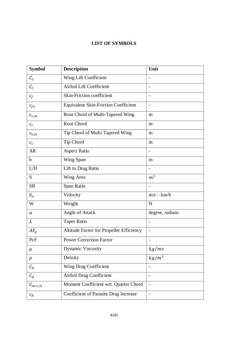
LIST OF SYMBOLS
Symbol Description Unit
𝐶𝐿 Wing Lift Coefficient -
𝐶𝑙 Airfoil Lift Coefficient -
𝑐𝑓 Skin-Friction coefficient -
𝑐𝑓𝑒 Equivalent Skin-Friction Coefficient -
𝑐𝑟,𝑚 Root Chord of Multi-Tapered Wing m
𝑐𝑟 Root Chord m
𝑐𝑡,𝑚 Tip Chord of Multi-Tapered Wing m
𝑐𝑡 Tip Chord m
AR Aspect Ratio -
b Wing Span m
L/D Lift to Drag Ratio -
S Wing Area 𝑚2
SR Span Ratio -
𝑉∞ Velocity m/s – km/h
W Weight N
𝛼 Angle of Attack degree, radians
𝜆 Taper Ratio -
𝐴𝐹𝜂 Altitude Factor for Propeller Efficiency -
PcF Power Correction Factor -
𝜇 Dynamic Viscosity 𝑘𝑔 𝑚𝑠⁄
𝜌 Density 𝑘𝑔/𝑚3
𝐶𝐷 Wing Drag Coefficient -
𝐶𝑑 Airfoil Drag Coefficient -
𝐶𝑚 ,𝑐/4 Moment Coefficient wrt. Quarter Chord -
𝑐𝐾 Coefficient of Parasite Drag Increase -

xxiii
LIST OF ABBREVIATIONS
Abbreviation Description Unit
AGL Above Ground Level m
AMSL Above Mean Sea Level m
BLOS Beyond Line of sight -
DFMA Design for Manufacturing and Assembly -
DGCA Directorate General of Civil Aviation -
EPS Expanded Polystyrene -
ISR Intelligence Surveillance and Reconnaissance -
LOS Line of Sight -
Mini UAV Miniature UAV -
MSL Mean Sea Level m
MTOM Maximum Take-off Mass kg
MTOW Maximum Take-off Weight N
MUAV Mini Unmanned Aerial Vehicle -
RPV Remotely Piloted Vehicle -
SAM Surface to Air Missile -
SHT-İHA İnsansız Hava Aracı Sistemlerinin Ayrılmış Hava
Sahalarındaki Operasyonlarının Usul ve Esaslarına İlişkin
Talimat
-
UAS Unmanned Aerial System -
UAV Unmanned Aerial Vehicle -
XPS Extruded Polystyrene -
wrt. with respect to -
MUAS Mini Unmanned Aerial System -
UAS Unmanned Aerial System -
RTM Resin Transfer Molding -
PHA Positive High Angle of Attack -
PLA Positive Low Angle of Attack -

xxiv
CFD Computational Fluid Dynamics -
HAD Hesaplamalı Akışkanlar Dinamiği -
RPM Revolution per Minute -
rps Revolution per Second -

1
CHAPTER 1
INTRODUCTION
1. INTRODUCTION
1.1. Unmanned Aerial Vehicles
Unmanned aerial vehicles (UAV) are mainly designed and operated to minimize
operational costs and eliminate risks of life losses during aerial missions such as
surveillance, reconnaissance and military operations. Especially for the military
operations called "D-cube" (Dangerous-Dirty-Dull) [1] risks of life loss is the main
problem and UAV's are the most appropriate solution at these situations.
Furthermore, practical mission time or endurance of a UAV may be much higher
than human pilots, which is impossible to sustain mission for a human pilot such a
long time.
Types of the UAV's can be categorized in two different terms, functional usage and
size i.e. range/altitude. Functionally, mission capability is the criteria, which are
target and decoy, reconnaissance-surveillance, combat, logistics, research and
development, civil and commercial UAV's [2]. In terms of size categorization, range
and altitude parameters lead to determine the size of the aircraft. Classification table
in terms of mission radius and altitude is given in Table 1.1 [3].

2
Table 1.1. NATO UAS Classification Guide [3]
Categories Category Operating
Altitude Mission Radius
CLASS 1
(<150kg)
Micro (<2 kg) <200 ft AGL 5 km (LOS)
Mini (2-20 kg) <3000 ft AGL 25 km (LOS)
Small (>20 kg) <5000 ft AGL 50 km (LOS)
CLASS 2
(150 kg-600 kg) Tactical <10000 ft AGL 200 km (LOS)
CLASS 3
(>600 kg)
MALE <45000 ft MSL >200 km (BLOS)
HALE <65000 ft MSL BLOS
Strike/Combat <65000 ft MSL BLOS
1.2. History of Unmanned Aerial Vehicles
Unmanned aerial vehicle (UAV) is basically a flying vehicle without a human pilot
aboard. In order to operate a UAV, autonomous flight system or remote control is
needed to control flight attitude. During the early years, mechanical and gyroscopic
devices are used to control attitude of the flying vehicle. Hewitt-Sperry Automatic
Airplane, shown in Figure 1.1, better known as the Sperry “Flying Bomb” is
regarded as the grandfather of modern UAV’s and cruise missiles. Flight attitude is
controlled by a gyro based mechanical autopilot which has a capability to hit
predefined targets [5].
Figure 1.1. Sperry “Flying Bomb” [5]
3
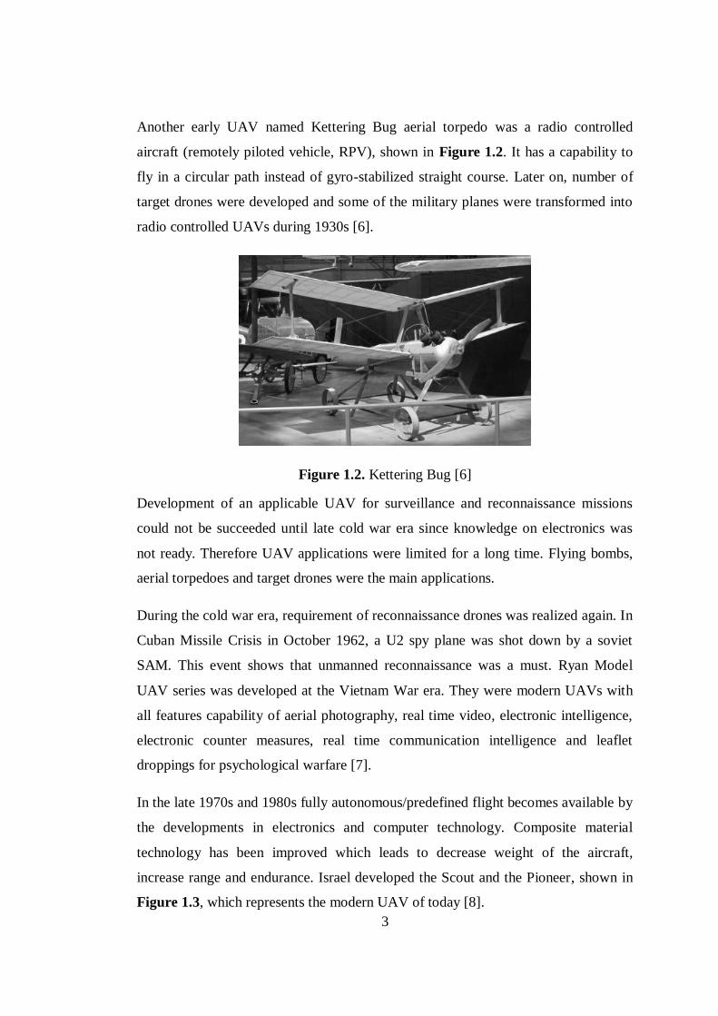
Another early UAV named Kettering Bug aerial torpedo was a radio controlled
aircraft (remotely piloted vehicle, RPV), shown in Figure 1.2. It has a capability to
fly in a circular path instead of gyro-stabilized straight course. Later on, number of
target drones were developed and some of the military planes were transformed into
radio controlled UAVs during 1930s [6].
Figure 1.2. Kettering Bug [6]
Development of an applicable UAV for surveillance and reconnaissance missions
could not be succeeded until late cold war era since knowledge on electronics was
not ready. Therefore UAV applications were limited for a long time. Flying bombs,
aerial torpedoes and target drones were the main applications.
During the cold war era, requirement of reconnaissance drones was realized again. In
Cuban Missile Crisis in October 1962, a U2 spy plane was shot down by a soviet
SAM. This event shows that unmanned reconnaissance was a must. Ryan Model
UAV series was developed at the Vietnam War era. They were modern UAVs with
all features capability of aerial photography, real time video, electronic intelligence,
electronic counter measures, real time communication intelligence and leaflet
droppings for psychological warfare [7].
In the late 1970s and 1980s fully autonomous/predefined flight becomes available by
the developments in electronics and computer technology. Composite material
technology has been improved which leads to decrease weight of the aircraft,
increase range and endurance. Israel developed the Scout and the Pioneer, shown in
Figure 1.3, which represents the modern UAV of today [8].

4
Figure 1.3. IAI - RQ-2 Pioneer [8]
Starting from the Scout and Pioneer, numerous modern unmanned aerial systems has
been developed and categorized in terms of different mission capabilities and sizes
mentioned in previous section. However, reciprocating engines and preliminary
electronics restrained to make smaller UAV. Small/Mini/Micro UAV concept is
improved by the developments in electronics, electric motor, servo and battery
technologies. Although small and some mini UAVs are still powered by a small
reciprocating engine, efficient electric motor-battery power systems allows to make
remarkably smaller aircraft possible. Miniaturization reduces cost and detection
risks, increases survivability.
1.3. Mini UAVs
Mini UAVs are the UAV class with 2-20 kg operational weight, which can be carried
by a personal to the operation field. Mission radius is the line of sight (LOS) which is
about 25 km and 3000 ft operational altitude above the ground (AGL) with 1-2 hour
endurance [3], [9]. The most advantageous feature of the mini UAV is the low cost
and expandability compared to the Class 2 and Class 3 UAVs mentioned in Section
1.1. Mini UAVs are generally used in close range ISR missions, target detection and
identification for the military purposes and less amount of crew and less training are
needed to operate as shown in Figure 1.4.

5
Figure 1.4. ISR Mission Performed by a Single Operator [10]
Besides military missions, mini UAVs are used for civilian purposes like scientific
research, disaster prevention and management, environmental protection, homeland
security, communication missions, protection of critical infrastructure. Current
situation in European UAS market shows that Small and Mini UAVs (S/MUAS)
dominate the civilian market as shown in Figure 1.5 [11].
Figure 1.5. Civilian Market for UAS in Europe by Category 2008-2017 [11]

6
1.4. Demircan Mini UAV
Demircan Mini UAV is a portable mini UAV, designed as a scope of this thesis
work. Aircraft is designed to operate in 10 km mission radius, 3000 m service
ceiling, 1.5 hour of endurance with 1.5 kg payload. Maximum takeoff weight is 4 kg.
As a design requirement, man-portable design and multi-mission capability is also
considered. For that reason, main parts of the aircraft can be easily mounted and
demounted and placed in a case carried by a personal to the operation field. In order
to provide multi-mission capability, two different design features exist.
The first design feature is the body ports under the fuselage which allow mounting
different landing gear configurations to adapt different operational environments. If
there is a smooth runway on the operation field, tricycle type landing gear can be
attached for the conventional takeoff and landing. Hook attachment allows catapult
launch and slide-landing on these hooks in order to achieve safe takeoff under harsh
environmental conditions if desired. Additionally, if the field is not suitable for the
conventional takeoff or catapult launch, hand launch option may be considered since
maximum takeoff weight of the aircraft allows achieving 8 to 9 m/s hand launch
takeoff speed. In order to achieve safe hand launch and prevent operators hand from
injury since the propeller clearance is low, a hand guard may be attached to the aft
body.
The other feature to provide multi-mission capability is the “Mission Compartment"
which is the top front part of the fuselage. This compartment includes the nose part
of the aircraft in order to carry camera gimbal / mechanism or experimental devices
etc. Remaining part of the Mission Compartment may include internal power supply
of the mission kit, video transmitter, antennas, sensors, data acquisition unit etc.
Mission compartment may be designed particularly in line with desired mission
requirements.
Stationary components of the aircraft like batteries, mission computer / autopilot
card, receiver etc. are attached to the bottom and aft part of the fuselage. This section
is structurally strongest part of the aircraft since it includes wing-body joints, mission
compartment joints and landing gear ports.
7
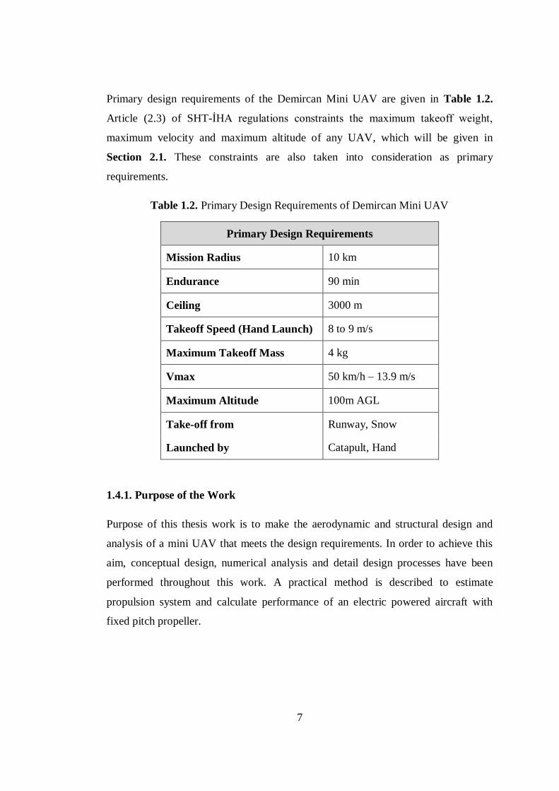
Primary design requirements of the Demircan Mini UAV are given in Table 1.2.
Article (2.3) of SHT-İHA regulations constraints the maximum takeoff weight,
maximum velocity and maximum altitude of any UAV, which will be given in
Section 2.1. These constraints are also taken into consideration as primary
requirements.
Table 1.2. Primary Design Requirements of Demircan Mini UAV
Primary Design Requirements
Mission Radius 10 km
Endurance 90 min
Ceiling 3000 m
Takeoff Speed (Hand Launch) 8 to 9 m/s
Maximum Takeoff Mass 4 kg
Vmax 50 km/h – 13.9 m/s
Maximum Altitude 100m AGL
Take-off from Runway, Snow
Launched by Catapult, Hand
1.4.1. Purpose of the Work
Purpose of this thesis work is to make the aerodynamic and structural design and
analysis of a mini UAV that meets the design requirements. In order to achieve this
aim, conceptual design, numerical analysis and detail design processes have been
performed throughout this work. A practical method is described to estimate
propulsion system and calculate performance of an electric powered aircraft with
fixed pitch propeller.

8
1.4.2. Scope of the Work
Mission profile for an electric powered mini UAV is defined and design phases are
described. One of the most important phases of this thesis work is to come up with
different structural designs for the wing and wing structural analyses in order to
examine structural design - strength - weight relations of typical wing designs for
mini UAVs and model aircraft. In order to perform structural analysis of the wing,
computational fluid dynamics (CFD) analysis of the wing at limit load condition is
considered. Comprehensive CFD analysis of the design is not within the scope of this
thesis. By taking structural behavior into account, one of these candidate
configurations is selected as the final structural configuration. However, structural
analyses of the fuselage and tail are not covered by this study. At the end of this
work, design of the Demircan Mini UAV will be ready to be manufactured from
composite materials.
1.4.3. Contributions
Although the design process of a fuel consuming conventional aircraft is well
established, determination of propulsion system efficiency and fixed-pitch propeller
thrust with respect to flight velocity and altitude is the major challenge for an electric
powered aircraft design since the propulsion system of small UAVs account for as
much as 60% of the overall weight [12]. As a first contribution, practical power
available and dynamic thrust estimation method for a fixed-pitch propeller powered
by an electric motor is presented in the conceptual design chapter of the thesis.
In the numerical analysis chapter, common wing structure configurations with
composite materials are investigated. Wing configurations with I-Beam and carbon
tube spars are structurally analyzed in order to understand structural load distribution
due to aerodynamic loads. By this way, structural advantages or disadvantages of
these designs can be examined which is the other contribution of the thesis.

9
1.4.4. Design Methodology
Design methodology of this work includes three main phases. These are the
conceptual design phase, numerical analysis and structural design of the wing and
detail design of the aircraft. Conceptual design is an iterative phase, where design
requirements are checked by performance and constraint analyses. In the numerical
analysis phase, CFD analysis of the wing is performed for the limit load defined in
the conceptual design phase. Structural configurations for the wings are defined and
structural analyses of the wing structure configurations are performed by using
referenced material definitions [38]. Finally, structural layout of the wing is decided
at the end of the numerical analysis chapter. Overall design and sub-components of
the aircraft are specified in the detail design phase. Overall weight of the design is
checked, since the MTOW of the aircraft is constrained by Article (2.3) of SHT-İHA
regulations [13]. Design for manufacturing and assembly, portability and ease of
manufacturing issues are also explained in the detail design phase. Finally design of
the aircraft is completed at the end of this study and ready to be manufactured design
is presented. Figure 1.6 shows the design flowchart followed in the study.

10
Figure 1.6. Design Flowchart
START
CONCEPTUAL
DESIGN
DETAIL DESIGN
END
NUMERICAL
ANALYSIS
Wing Loading
Material Definitions
Structural Analysis of
Candidate Wing Designs
CFD Analysis
Wing Structure Design
Assembly Design
Detailed Structural Design
Weight Check
Configuration Layout
Airfoil Selection and
Wing Sizing (W/S)
Fundamental Parameters
(CL,max, CD0, K, e)
Constraint Analysis (PA/W)
Performance Analysis
Aircraft Performance Parameters
Climb Performance
Gliding and Handlaunch
Takeoff Distance
Range and Endurance
V-n Diagram
Design Requirements
Dynamic Thrust Estimation
Motor-Propeller Selection
Experiment
Dynamic Thrust wrt. Altitude
Power Available wrt. Altitude
Longitudinal Stability Analysis
Overall Sizing
Constraint Analysis (P/W)
Components and
Weight Distribution

11
CHAPTER 2
CONCEPTUAL DESIGN
2. CONCEPTUAL DESIGN
2.1. Introduction
Conceptual design of Demircan Mini UAV is established in this chapter. Design
requirements are defined, configuration layout is specified, aircraft performance
calculations are accomplished, system components are specified and finally
conceptual design is determined. Improved aerodynamic relations and dynamic
thrust model specified for electric motor with fixed-pitch propeller are presented.
Additionally range and endurance relations for battery powered aircraft are referred
to determine required battery capacity for electric powered aircraft. In order to
achieve much more reliable design these relations are used in aircraft performance
calculations. At the end of this chapter conceptual design is completed.
2.2. Regulations
Regulations of Directorate General of Civil Aviation (DGCA) of Turkey are taken
into consideration before deciding the design requirements of the UAV, which is
named SHT-İHA. According to Article (4.ş) of SHT-İHA, except from model
aircraft used for sport or entertainment, any unmanned flying vehicle capable of
autonomous flight or controlled by a ground operator is defined as a UAV. This
regulation contains important rules like operational permissions, operator
responsibilities, airworthiness requirements, safety rules, air traffic control issues and
pilot licensing and proficiency requirements for UAV operations.
In order to design and operate a UAV beyond the scope of this regulation, maximum
takeoff mass (MTOM), maximum velocity and maximum altitude (AGL) constraints
should be considered as stated in Article (2.3) of SHT-İHA. Table 2.1 gives the

12
SHT-İHA constraints. Any UAV, which does not obey these constraints, are
subjected to the SHT-İHA regulations and operational permissions should be taken
from DGCA of Turkey [13].
Table 2.1. SHT-İHA Constraints
MTOM 4 kg
Vmax 50 km/h – 13.9 m/s
Maximum Altitude 100m AGL
2.3. Design Requirements
Fixed wing Mini UAVs have a wide range of usage and they may be used in almost
all environments including high altitude mountains to sea level operations for civil or
military purposes. For that reason, ceiling and operational environment will be
considered to design the aircraft. Design altitude should be chosen as high as
possible and general design layout will be chosen for the desired operational and
environmental conditions.
In order to design a mini UAV which can operate in different operational
environments, firstly portability issues should be considered for the mobility. In the
second place, takeoff and landing configuration of the aircraft should be appropriate
for different types of operational fields and in the current study replaceable landing
gear configuration is chosen for the design. Conventional landing gear can be
attached for runway takeoff and landing and hook attachment can be used for
catapult launches, in order to achieve required takeoff speed in safe. Design
configuration and MTOW of the aircraft also allows achieving 8-9 m/s hand launch
takeoff speed for an average operator.
Payload of the aircraft is a mission compartment up to 1.5 kg which is chosen for the
multi-mission capability of the design. Mission radius and endurance are 10 km and
90 min of flight time at 3000 m operational altitude. Additionally, SHT-İHA
constraints should be followed.

13
Table 2.2 gives the general design requirements of Demircan Mini UAV where
SHT-İHA constraints are added into the preliminary design requirements given in
Table 1.2.
Table 2.2. General Design Requirements of Demircan Mini UAV
General Designs Requirements
Hand Launch Takeoff Velocity 8-9 m/s
Takeoff Runway, Catapult, Hand
Payload (Mission Compartment) 1.5 kg
Mission Radius 10 km
Endurance 90 min
Ceiling 3000 m
MTOM 4 kg
Vmax 50 km/h
Maximum Flight Altitude 100m AGL – 3000 m AMSL
2.3.1. Mission Profile
Mission profile of the aircraft is performed in 10 km mission radius with 90 minutes
of endurance and 100 m AGL operational altitude up to 3000 m AMSL elevation.
Takeoff - Cruise – Loiter - Return Cruise and Landing phases are the main phases of
the mission profile. Loiter phase is implemented according to the chosen mission kit
such as surveillance and reconnaissance, surface mapping or atmospheric data
collection etc. Sample mission profile is plotted in Figure 2.1.
Figure 2.1. Mission Profile

14
At station 0, pre-flight inspections, such as connections, flight control surfaces,
ground control units etc. are performed. Climb to 100 m AGL altitude is performed
between stations 0-1 at maximum rate of climb condition and cruise is performed
between stations 1-2 and 3-4 (return cruise) at (𝐿/𝐷)𝑚𝑎𝑥 value for propeller driven
airplanes and maximum propeller efficiency condition in order to maximize range.
Since fixed-pitch propeller has the maximum efficiency at a unique advance ratio
value, which is the ratio of the design speed and the RPM value of the propeller,
selecting a proper propeller that fits the design becomes significant for the cruise
flight. Loitering is performed between stations 2-3 at maximum endurance condition
(𝐿3/2/𝐷)𝑚𝑎𝑥
for propeller driven airplane, where flight time is more important than
range in this phase. After the return cruise, descending phase to the landing zone is
performed between stations 4-5. Flying at cruise and loiter conditions are not only
related with proper propeller selection but also related with compatible electric motor
selection where current drain is also be needed to minimized at these flight phases in
order to achieve longer range and endurance values. Therefore actual cruise and
loiter speeds are determined from range and endurance calculations for battery
powered aircraft.
2.3.2. Competitor Study
Competitor study is performed in order to obtain initial sizing and performance
parameters referring to the present designs that match the desired design
requirements. Conventional mini UAV designs are classified according to their
fuselage and propulsion types which are Boom-Tractor, Cargo-Pusher and Cargo-
Tractor types. Boom type fuselage is the simplest design where wing, tail and
payloads are attached to the boom. For the cargo type fuselage, flight system and
equipment are placed in a fuselage and wing and tail are attached on the fuselage.
Second classification name is the propulsion configuration as tractor and pusher.
Layout classifications are shown in Table 2.3 and some of competitor aircraft are
listed with their pictures as examples and all competitors are listed in Table 2.4.

15
Table 2.3. Layout Classification for Mini UAVs
Boom-Tractor Cargo-Pusher Cargo-Tractor
Elbit -Skylark 1 Baykar - Bayraktar METU – Güventürk
(Referenced in Appendix A)
Table 2.4. Layout Classification of Competitor Mini UAVs.
Boom - Tractor Cargo - Pusher Cargo - Tractor
Elbit - Skylark 1 AV- Pointer AV - Puma AE
ST Aero - Skyblade 3 Hydra Tech. - E1 Gavillan METU - Güventürk
Top I Vision - Casper 250 Nostromo - Cabure 2
Tasuma - Hawkeye 2 Baykar - Bayraktar
MKU - Terp2
Tasuma - Hawkeye 3
Average design parameters are given in the Table 2.5. Design specifications and
references of competitors are given in Appendix A.
Table 2.5. Average Design Parameters of Competitor Mini UAVs
Average Design Parameters of
Competitor mini UAVs
MTOW 4.23 kg
Wing Span 2.12 m
Length 1.46 m
Cruise Velocity 16.1 m/s
Ceiling 2790 m
Mission Radius 9.5 km
Endurance 80 min

16
ISR missions are the primary objective of mini UAVs for the military applications.
Thus, gimbal systems for mini UAVs are also researched and one of them is selected
as a candidate for the conceptual design phase. Selected gimbal has object tracking,
high definition streaming, real time video stabilization and geo-lock capabilities [14].
Total payload for a gimbal system with power units, transmitter etc. is assumed as
1.5 kg. Figure 2.2 shows the selected gimbal and specifications of the selected
gimbal are given in Table 2.6.
Figure 2.2. UAV Vision CM100 Gimbal [14]
Table 2.6. UAV Vision CM100 Specifications [14]
Mass - Weight 0.800 kg – 7.85 N
Dimensions Diameter : 100 mm
Length/Height : 129 mm
Power / Voltage 12W / 9-36 V

17
2.3.3. Initial Design Parameters
Initial design parameters of Demircan mini UAV is specified and given in Table 2.7
by using competitor averages given in Table 2.5.
Table 2.7. Initial Design Parameters of Demircan Mini UAV
Competitor Averages
Demircan
Mini UAV
Wing Span :b 2.12 m 2.2 m/s
Wing Area: S* 0.484 m2 0.605 m
2
Mean Chord: c* 0.228 m 0.275 m
Aspect Ratio: AR 9.27 - 8 -
Length 1.46 m 1.5 m
MTOW 4.23 / 41.5 kg / N 4 / 39.24 kg / N
Payload 0.95 - 1.5 kg 1.5 kg
Vmax 26.6 m/s - m/s
Vcruise 16.1 m/s 13.9 m/s
Vstall 11.7 m/s 8 - 9 m/s
Ceiling 2790 m 3000 m
Endurance 80 min 90 min
Mission Radius 9.5 km 10 km
(*Calculated from related parameters)
2.4. Configuration Layout
Layout class of the Demircan mini UAV is Cargo-Pusher as mentioned in Section
2.3.2. While choosing the Fuselage-Propulsion class operational advantages and
disadvantages, manufacturability issues, performance and stability characteristics are
taken into account.
Boom-Tractor type is a simple design but payload/camera pod is generally placed
under the fuselage because of the stability issues and mostly propeller blocks the
frontal view of the camera. Also, during the landing, camera is the first contact point
of the aircraft to the ground. Also there is limited place to locate electronic system in
the pod. This configuration allows hand launch but mounting different landing gears
on the payload pod is not practical.

18
Cargo-Tractor type is a conventional design but the most important problem is the
location of the camera and payload. Camera should be located under the fuselage and
it needs extra precaution mechanisms like retractable camera mechanism or camera
door to protect camera system during belly landings. Locating camera system far
from the motor in order to enhance monitoring quality due to magnetic interference
and vibration of the motor is the other important issue.
Cargo-Pusher type is advantageous for the monitoring since the camera system can
be placed at the front of the fuselage. The greatest advantage is airflow over the wing
is undisturbed and camera has a clear view. Additionally, undisturbed air flow is
preferred for the experimental payload especially for the atmospheric data
measurement missions. Protective cautions like nose shield may still be needed for
belly landings in order to protect nose camera. Twin boom mounted tail to the wing
configuration like in most of the tactical UAVs can be preferred in order to reduce
fuselage height and length. By this way, fuselage drag can be reduced and mobility
can be increased. Moreover, fuselage can be designed separately for each mission
configuration, which allows a flexible design envelope for the fuselage and it is
advantageous for the multi-mission concept. For this thesis work, “mission
compartment” is considered as the replaceable part of the aircraft. As a result, cargo
type fuselage with pusher propeller and twin boom - high tail configuration is chosen
for design.
2.4.1. Design Configuration of the Demircan Mini UAV
Fuselage has a rounded box shape with high conic aft in order to keep pusher
propeller high as possible and improve propeller clearance. High wing configuration
is chosen in order to improve the grip of the body for hand launch and stability of the
aircraft.
Tail booms are mounted on the hard points of the wings at the end of the rectangular
root section for the structural rigidity of tail and boom ports. Twin vertical tails are
placed to the boom end junctions and high tail is placed to the vertical tail tips.

19
Pusher type propeller configuration is chosen in order to place the camera system at
the nose for clear view and undisturbed airflow for the experimental mission
compartment. The most important disadvantage of this propeller configuration is low
propeller clearance during hand launch and landing. Propeller guard placed to the aft
fuselage may be helpful for hand launch and belly landing cases.
Conventional landing gear and hook attachments may be placed to the body ports
under the fuselage for safe takeoff and landing as an option. Figure 2.3 shows the
conceptual design of Demircan Mini UAV.
Figure 2.3. Design Configuration of Demircan Mini UAV
2.5. Airfoil Selection and Wing Sizing
Airfoil of the wing is selected by considering design requirement for the maximum
lift coefficient and Reynolds number of the wing at the design speed and altitude
range. Required maximum lift coefficient of the airfoil is calculated for stall
conditions at different operational altitudes. After selecting the airfoil, maximum lift
coefficient of the finite wing, which is the fundamental design parameter of the
conceptual design phase, is determined. Standard atmosphere parameters, shown in
Table 2.8, are used for the lift coefficient and Reynolds number calculations.

20
Table 2.8. Standard Atmosphere Table (AMSL)
Altitude
m
Density
𝝆∞
𝒌𝒈 𝒎𝟑⁄
Dynamic Viscosity
𝝁∞
𝒌𝒈 (𝒎 ⋅ 𝒔⁄ )
0 1.2250 1.789 x10⁻⁵
500 1.1673 1.774 x10⁻⁵
1000 1.1117 1.758 x10⁻⁵
1500 1.0581 1.742 x10⁻⁵
2000 1.0066 1.726 x10⁻⁵
2500 0.9570 1.710 x10⁻⁵
3000 0.9093 1.694 x10⁻⁵
2.5.1. Lift Coefficients
Selected airfoil should satisfy the lift requirement for stall and cruise conditions,
which is the MTOW of the aircraft. Stall speed is selected as 8 m/s at 1000 m and 9
m/s at 3000 m. 𝑪𝑳,𝒎𝒂𝒙 and 𝑪𝑳,𝒄𝒓𝒖𝒊𝒔𝒆 requirements for the candidate airfoil are
calculated from Eqn. (2.1) and Table 2.9 gives the lift coefficient requirements at
different speeds and altitude.
𝐿 =1
2𝜌∞𝑉∞
2𝑆𝐶𝐿 (2.1)
𝐶𝐿,𝑚𝑎𝑥 =2𝑊
𝜌∞𝑉𝑠𝑡𝑎𝑙𝑙2 𝑆
(2.2)
𝐶𝐿,𝑐𝑟𝑢𝑖𝑠𝑒 =2𝑊
𝜌∞𝑉𝑐𝑟𝑢𝑖𝑠𝑒2 𝑆
(2.3)
Where W=39.24 N and S=0.605 m2.
Table 2.9. Lift Coefficient Requirements at Different Speeds and Altitude
CL
V 0m 1000m 2000m 3000m
8 m/s (Stall) (High Aoa) 1.655 1.823 2.014 2.229
9 m/s (Stall) (High Aoa) 1.307 1.441 1.591 1.761
13.9 m/s (Cruise) (Low Aoa) 0.548 0.604 0.667 0.738

21
Figure 2.4. Maximum Lift Coefficients for Different Stall Velocities
As can be seen from Figure 2.4, although 𝑪𝑳,𝒎𝒂𝒙 of the selected airfoil should be at
least 1.823 for 1000m operational altitude, required lift coefficient at 8-9 m/s stall
speed range for different operational altitudes is selected as 1.8. Similarly, cruise lift
coefficient at low angle of attack should be between 0.55 and 0.74 as given in Table
2.9 in order to minimize drag at cruise condition.
2.5.2. Reynolds Number
Reynolds number range of the wing is calculated considering the 0 m to 3000 m
altitude range, and stall speeds (8-9 m/s) and the design cruise speed. Table 2.10
gives the Reynolds number ranges at different operational altitudes.
𝑅𝑒 =𝜌∞𝑉∞𝑐
𝜇∞ (2.4)
𝑉𝑠𝑡𝑎𝑙𝑙 = 8𝑚 𝑠⁄ , 𝑉𝑐𝑟𝑢𝑖𝑠𝑒 = 13.9 𝑚/𝑠, 𝑐 = 0.275 𝑚
Table 2.10. Reynolds Number Range
Reynolds Number 0m 1000m 2000m 3000m
Vstall = 8 m/s 150642.8 139120.6 - -
Vstall = 9 m/s - - 144341.5 132852.3
Vcruise = 13.9 m/s 261741.9 241722 222927.5 205183

22
Based on the results given in Table 2.10, Reynolds number range of the design is
taken to be 130000 – 260000.Therefore, airfoil search is performed within this range.
Nominal Reynolds number is selected for the operational cruise altitudes between
1000 m-2000 m as 230000.
2.5.3. Airfoil Analyses
MH114 airfoil is selected between vast number of low speed / low Reynolds number
airfoils. Candidate airfoils are analyzed for the nominal Reynolds number
(𝑅𝑒𝑛𝑜𝑚𝑖𝑛𝑎𝑙 ≈ 230000) by using XFLR5 – XFOIL Direct Analysis module [16].
XFOIL is a widely used interactive program/module for the design and analysis of
subsonic isolated airfoils. Viscous or inviscid analysis capabilities of the tool allows
forced or free transition, transitional separation bubbles, trailing edge separation,
compressibility correction and lift-drag predictions [17]. Therefore determination of
airfoil characteristics is relied on XFLR5 – XFOIL analysis results. Lift coefficient
analysis results of four candidate airfoils are shown Figure 2.5.
Figure 2.5. Cl vs. Alpha Curves of Candidate Airfoils at Re=230000

23
From Figure 2.5 (Cl vs. Alpha Curve), MH113 and MH114 airfoils are selected as
the final candidates since lift coefficient at zero angle of attacks are satisfactory and
maximum lift coefficient of these airfoils are close to 𝐶𝐿,𝑚𝑎𝑥 = 1.8. Maximum lift
coefficient of the finite wing is lower than the 2D airfoil due to finite wing-body
losses. It is seemed to be unsatisfactory for the maximum lift coefficient requirement
to satisfy lift requirement at 8-9 m/s stall speeds but flapped wing configuration is
considered for different operational altitudes in order to minimize wing drag at level
flight phases. Lift to drag ratio (Cl/Cd) is the critical parameter on deciding the
airfoil. Selected airfoil should have the highest lift and at the same time it should
have the lowest drag. Therefore, airfoil with the highest Cl/Cd value is the most
appropriate choice for the design. Cl/Cd results are shown in Figure 2.6.
Figure 2.6. Cl/Cd vs. Alpha Curves of Candidate Airfoils at Re=230000

24
From Figure 2.6, Cl/Cd value of MH114 is higher than MH113 since MH114 airfoil
is thinner, which is also better for low Reynolds number flight regime. Hence,
MH114 airfoil is selected for the design and shown in Figure 2.7.
Figure 2.7. MH114 Airfoil
Cl vs. angle of attack curve of the MH114 airfoil at Reynolds number 230000 is
shown in Figure 2.8.
Figure 2.8. Cl vs. Alpha Curve of MH114 at Re=230000
Figure 2.8 shows that maximum lift coefficient 𝑪𝒍,𝒎𝒂𝒙is 1.75 at 13.5 degree angle of
attack. Cl/Cd vs. angle of attack and Cm,c/4 vs. angle of attack curves of MH114 at
Re=230000 are given in Figure 2.9 and Figure 2.10 respectively. Cl/Cd has the
maximum value at 5 degree angle of attack as shown in Figure 2.9 and moment
coefficient at quarter chord is about -0.18 at low angle of attacks as shown in Figure
2.10.

25
Figure 2.9. Cl/Cd vs. Alpha Curve of MH114 at Re=230000
Figure 2.10. Cm,c/4 vs. Alpha Curve of MH114 at Re=230000

26
Table 2.11 summarizes aerodynamic coefficients of the MH114 Airfoil. Lift
coefficient of the finite wing (𝑪𝑳) and maximum lift coefficient of the flapped wing
(𝑪𝑳,𝒎𝒂𝒙) are discussed in the following section.
Table 2.11. Aerodynamic Coefficients of the MH114 Airfoil.
𝑪𝒍,𝒎𝒂𝒙 = 1.75 @ 𝛼 = 13.5°
𝑪𝒍,𝜶=𝟎 = 0.83 @ 𝛼 = 0°
𝑪𝒍,𝑳=𝟎 = 0 @ 𝛼 = −9.5°
(𝑪𝒍 𝑪𝒅⁄ )𝒎𝒂𝒙 = 88 @ 𝛼 = 5°
𝒄𝒎,𝒄 𝟒⁄ = -0.18 At low AOA.
2.5.4. Stall Constraint and Wing Loading
Stall constraint is the most important requirement for hand launch. 𝐶𝐿,𝑚𝑎𝑥 is
specified as 1.8 in the previous section. Initial wing sizing is needed to be updated
and flap size should be determined to achieve the required lift coefficient. It should
be noted that wing loading and wing area are the fundamental constraints for the
wing sizing at this point. Stall constraints are minimum wing area required and
maximum wing loading for 8m/s stall speed at 1000 m altitude.
(𝑊
𝑆)𝑠𝑡𝑎𝑙𝑙
=1
2𝜌∞𝑉𝑠𝑡𝑎𝑙𝑙
2 𝐶𝐿,𝑚𝑎𝑥 (2.5)
(𝑊
𝑆)𝑠𝑡𝑎𝑙𝑙
= 64.034 𝑁/𝑚2
𝑆𝑚𝑖𝑛 =𝑊
(𝑊/𝑆)=39.24
64.034= 0.613 𝑚2
Wing dimensions are re-calculated for the new wing loading parameter, where
AR=8.
𝐴𝑅 = 𝑏2 𝑆⁄ (2.6)
𝑏 = √𝐴𝑅 ⋅ 𝑆 ≈ 2.22 𝑚
𝑆 = 2.222 8⁄ = 0.616 𝑚2
27
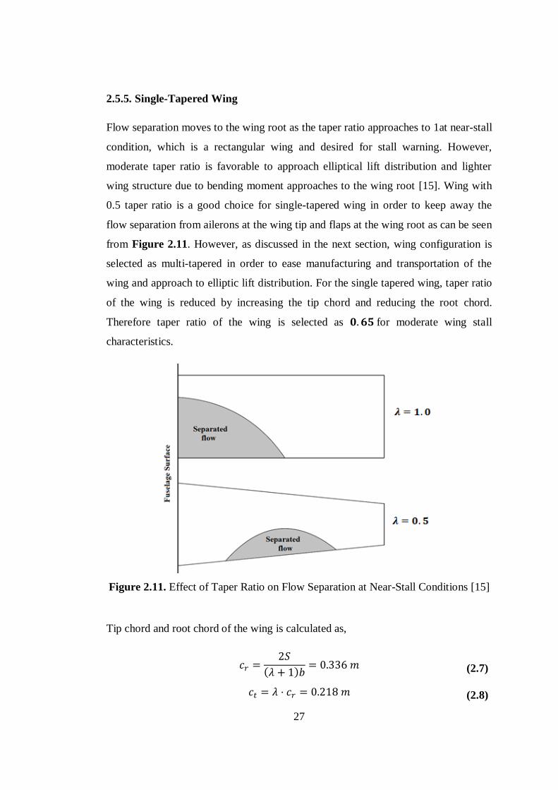
2.5.5. Single-Tapered Wing
Flow separation moves to the wing root as the taper ratio approaches to 1at near-stall
condition, which is a rectangular wing and desired for stall warning. However,
moderate taper ratio is favorable to approach elliptical lift distribution and lighter
wing structure due to bending moment approaches to the wing root [15]. Wing with
0.5 taper ratio is a good choice for single-tapered wing in order to keep away the
flow separation from ailerons at the wing tip and flaps at the wing root as can be seen
from Figure 2.11. However, as discussed in the next section, wing configuration is
selected as multi-tapered in order to ease manufacturing and transportation of the
wing and approach to elliptic lift distribution. For the single tapered wing, taper ratio
of the wing is reduced by increasing the tip chord and reducing the root chord.
Therefore taper ratio of the wing is selected as 𝟎. 𝟔𝟓 for moderate wing stall
characteristics.
Figure 2.11. Effect of Taper Ratio on Flow Separation at Near-Stall Conditions [15]
Tip chord and root chord of the wing is calculated as,
𝑐𝑟 =2𝑆
(𝜆 + 1)𝑏= 0.336 𝑚 (2.7)
𝑐𝑡 = 𝜆 ⋅ 𝑐𝑟 = 0.218 𝑚 (2.8)
28
Wing dimensions of the single-tapered wing are shown in Figure 2.12.
Figure 2.12. Single-Tapered Wing Dimensions
(Dimensions are in m)
2.5.6. Multi-Tapered Wing
Tip chord and root chord dimensions can be reduced by multi-tapering in order to
increase the mobility. Additionally, with multi-tapering approach wing shape and lift
distribution approaches to an elliptical wing. However, the effect of multi-tapering is
minor on lift distribution compared to the single-tapered wing. In the present study,
constant chord root section (rectangular) and tapered outer wing section is considered
for multi-tapering. Manufacturing of a multi-tapered wing is more complex than a
single-tapered wing for general aviation aircraft. On the contrary, multi-tapering is
considered to ease manufacturing and increase mobility by manufacturing
rectangular root section and tapered outer wings separately. In other words, the wing
consists of three separate parts as shown in Figure 2.13.
Figure 2.13. Multi-Tapered Wing
In the Figure 2.14, single-tapered and multi-tapered wings are shown together.
Reference area of single-tapered wing and multi-tapered wing are same, but root and
tip chord dimensions are reduced for the multi-tapered wing (gray). In Figure 2.14,
black areas are excess parts of the single-tapered wing.

29
Figure 2.14. Chord Reduction and Dimensions of the Multi-Tapered Wing
Dimensions of the multi-tapered wing are calculated with respect to the span ratio
(SR) parameter, which is the ratio of the rectangular span to the wing span. Span
ratio is zero for a single-tapered wing and one for a rectangular wing. Chord
distribution along half span of a single-tapered wing is given by
𝑐(𝑦) = 𝑐𝑟 − (𝑐𝑟 − 𝑐𝑡) (𝑦
𝑏/2) (2.9)
Root chord of the multi-tapered wing is the chord length at the wing span at
(SR/2)(b/2) as shown in Figure 2.14 and given by Eqn.(2.10).
𝑐𝑟,𝑚 = 𝑐𝑟 − (𝑐𝑟 − 𝑐𝑡) (𝑆𝑅
2) (2.10)
Total chord difference is same at the root and at the tip.
∆𝑐 = (𝑐𝑟 − 𝑐𝑡) (𝑆𝑅
2) (2.11)
𝑐𝑡,𝑚 = 𝑐𝑡 − Δ𝑐 (2.12)
𝑐𝑡,𝑚 = 𝑐𝑡 − (𝑐𝑟 − 𝑐𝑡) (𝑆𝑅
2) (2.13)
In the present study, span ratio is selected as 0.3.Tip chord, root chord and taper ratio
of the multi-tapered wing are calculated as,
𝑐𝑟,𝑚 = 0.336 − (0.336 − 0.218)(0.3
2) ≈ 0.318 𝑚

30
𝑐𝑡,𝑚 = 0.218 − (0.336 − 0.218) (0.3
2) ≈ 0.200 𝑚
𝜆 =𝑐𝑡,𝑚𝑐𝑟,𝑚
=0.318
0.200= 0.629
Final values of reference wing area and wing loading are determines as:
𝑆 = (𝑐𝑟,𝑚 ⋅ 𝑆𝑅 ⋅ 𝑏) + [(𝑐𝑟,𝑚 + 𝑐𝑡,𝑚) ⋅ (1 − 𝑆𝑅) ⋅ 𝑏 2⁄ ] = 0.614 𝑚2
𝑊
𝑆=39.24
0.614= 63.88 𝑁/𝑚2
Mean aerodynamic chord of a wing with variable chord is calculated as,
𝑐̅ =2
𝑆∫ 𝑐(𝑦)2 ⋅ 𝑑𝑦𝑏/2
0
(2.14)
Chord distributions along half span of a multi-tapered wing is divided into
rectangular and tapered sections, and they are calculated as,
𝑐1(𝑦) = 𝑐𝑟,𝑚 (2.15)
𝑐2(𝑦) = 𝑐𝑟,𝑚 − (𝑐𝑟,𝑚 − 𝑐𝑡,𝑚
(1 − 𝑆𝑅) ⋅ 𝑏/2) 𝑦 (2.16)
Eqn. (2.14) can be solved for rectangular and tapered sections separately yielding the
mean aerodynamic chord for the multi-tapered wing.
𝑐̅ =2
𝑆[∫ 𝑐1(𝑦)
2 ⋅ 𝑑𝑦𝑆𝑅.𝑏/2
0
+∫ 𝑐2(𝑦)2. 𝑑𝑦
(1−𝑆𝑅).𝑏/2
0
] (2.17)
𝑐̅ =b
𝑆[ SR ⋅ 𝑐𝑟,𝑚
2 + (𝑐𝑟,𝑚2 + 𝑐𝑟,𝑚 ⋅ 𝑐𝑡,𝑚 + 𝑐𝑡,𝑚
2)(1 − 𝑆𝑅)
3] (2.18)
𝑐̅ = 0.282 𝑚
Final wing dimensions and parameters are given in Table 2.12 and wing planform is
shown in Figure 2.15.

31
Table 2.12. Wing Parameters
Span: b 2.22 m
Aspect Ratio: AR 8
Span Ratio: SR 0.3
Taper Ratio: λ 0.629
Root chord: cr 0.318 m
Tip chord: ct 0.200 m
M.A.C. 0.282 m
S_wing, Sref 0.614 m2
W/S 63.88 N/m2
Swet_wing* 1.268 m2
(*:Wetted surface of the wing is determined from CAD drawing of the wing)
Figure 2.15. Multi-Tapered Wing Dimensions
(Dimensions are in m)

32
2.6. Preliminary Wing Analysis
In this section, finite wing analysis (FWA) of the multi-tapered wing is performed
with XFLR5 software. XFLR5 is an analysis tool for airfoils, wings and planes
operating at low Reynolds numbers [16]. It includes XFOIL’s [17] direct and inverse
airfoil analysis capabilities. Wing design and analysis capabilities of the tool are
based on Lifting Line Theory (LLT), Vortex Lattice Method with horseshoe vortex
(VLM1) and ring vortex (VLM2) options and 3D Panel Method.
Multi-tapered wing elements generated in XFLR5 are shown in Figure 2.16. 2D
VLM elements, analyzed in LLT and VLM, are automatically generated on the mean
camber line by projecting 3D panel elements generated on wing surfaces.
Figure 2.16. Wing Elements (3240 Panel Elements – 1600 VLM Elements)
Finite wing analyses are performed for LLT, VLM and 3D Panel Methods at 1000 m
and 13.9 m/s cruise condition. As can be seen from Figure 2.17, lift curves at small
angle of attacks are almost same but Panel Method gives higher lift coefficients.

33
VLM and Panel solutions do not converge near stall but stall behavior is detected
with LLT analysis and maximum lift coefficient results are almost same for all
solutions.
Figure 2.17. CL vs Alpha Results for 2D airfoil and 3D Wing Analyses.
Lift to drag ratio (𝐶𝐿 𝐶𝐷⁄ ) and moment coefficient at quarter chord (𝑐𝑚,𝑐/4) results
are also determined and plotted in Figure 2.18 and Figure 2.19, respectively.
Moment coefficient is selected from VLM analysis for which 𝑐𝑚,𝑐/4 is constant and
highest. Aerodynamic parameters selected from the results of wing analysis by
different solvers available in XFLR5 are summarized in Table 2.13.
Table 2.13. Aerodynamic Coefficients of the Multi-Tapered Wing
𝐶𝐿,𝑚𝑎𝑥 = 1.7 @ 𝛼 ≈ 15°
𝐶𝐿,𝛼=0 = 0.66 @ 𝛼 = 0°
𝐶𝐿,𝐿=0 = 0 @ 𝛼 = −8°
(𝐶𝐿 𝐶𝐷⁄ )𝑚𝑎𝑥 = 20.6 @ 𝛼 = 0°
𝑐𝑚,𝑐 4⁄ = -0.21

34
Figure 2.18. CL/CD Curves of Finite Wing Analysis Results.
Figure 2.19. Cmc/4 vs Alpha Results of Wing Analysis Results

35
Pressure coefficient (Cp) distribution on the wing is determined with the Panel
Method solution and results are shown in Figure 2.20 and Figure 2.21.
Aerodynamic load on the wing can be calculated by exporting mesh data and Cp
data. It may be reasonable to interpolate aerodynamic pressure data on the wing
structure in order to perform structural analysis. Reliability of pressure coefficient
results is discussed in Chapter 3, in which CFD analysis of the wing is performed.
Figure 2.20. Cp Distribution on the Upper and Lower Surfaces at 𝛼 = 0°.
Figure 2.21. Cp Distribution on Wing at 𝛼 = 0° (Isometric View)

36
Maximum required lift coefficient of the wing is 1.8 due to stall constraint. However,
maximum lift coefficient of the wing is determined as 𝑪𝑳,𝒎𝒂𝒙 = 𝟏. 𝟕 for the
unflapped condition. Therefore, high-lift device is needed to achieve stall velocity
requirement. Lift coefficient contribution of various high-lift devices are discussed
and tabled in the literature but in the present study, literature assumption is not
preferred since they are based on empirical relations on large aircraft. Therefore,
flapped wing conditions, which are taken as full span flap and 40% span flap
conditions with 30° deflection angle at 𝑉𝑠𝑡𝑎𝑙𝑙 = 8𝑚 𝑠⁄ , are analyzed to determine
more acceptable results. Analysis with higher deflection angles results with
convergence error due to high turbulence level. Therefore, 30° moderate flap
deflection angle is chosen for the takeoff condition. LLT analysis is preferred to
observe the lift decrement near stall condition. Wing models of wing without flap,
wing with full span plain flap and wing with 40% span plain flap conditions shown
in Figure 2.22 are analyzed for the cruise and the stall velocity conditions at 1000 m
altitude.
Figure 2.22. Flapped and Unlapped Wing Conditions
Lift coefficients vs. angle of attack curves of the flapped and unflapped conditions
are presented in Figure 2.23. Lift coefficient of 1.7 is again obtained for the multi-
tapered wing without flap as before and maximum lift coefficient of wing with full
flap is determined as 𝟏. 𝟗𝟓. Maximum lift coefficient is determined as 1.8 for the
multi-tapered wing with 40% spanwise flap as aimed. Analysis result for 𝐶𝐿,𝑚𝑎𝑥 is
also consistent with analytical calculation of 40% spanwise flap condition given by
Eqn. 2.19 [18].
𝐶𝐿,𝑚𝑎𝑥 = 𝐶𝐿 + 0.4 ⋅ Δ𝐶𝐿 = 1.70 + 0.4 ⋅ (1.95 − 1.70) = 1.80 (2.19)

37
Figure 2.23. CL vs. Alpha Results for LLT Analysis
Table 2.14 summarizes the maximum lift coefficient results obtained for flapped and
unflapped conditions.
Table 2.14. Lift Coefficient Table
Unflapped 𝐶𝐿,α=0° = 0.66 𝐶𝐿,𝑚𝑎𝑥 = 1.70
100% span flap, 𝛿 = 30° (𝐶𝐿,α=0°)100% = 1.175 𝐶𝐿,𝑚𝑎𝑥,100% = 1.95
40% span flap, 𝛿 = 30° (𝐶𝐿,α=0°)40% = 0.827 𝐶𝐿,𝑚𝑎𝑥,40% = 1.80
Another important result determined with wing analysis is CL vs CD relation of the
wing which is the drag polar. Aerodynamic coefficients and parameters at minimum
drag are important to determine aircraft performance relations. CL /CD vs angle of
attack results are shown in Figure 2.24 and drag polar result of the XFLR5 analysis
is shown in Figure 2.25.

38
Figure 2.24. CL/CD vs. Alpha Results for LLT Analysis
Figure 2.25. Drag Polar of the Wing

39
The following results are obtained from the drag polar and lift coefficient versus
angle of attack curves. Firstly, minimum drag value and corresponding lift
coefficient value are determined from the drag polar, then corresponding angle of
attack is determined from the lift coefficient curves.
𝑪𝑫,𝒎𝒊𝒏 = 𝟎. 𝟎𝟐𝟔 and (𝑪𝑳)𝒎𝒊𝒏𝒅𝒓𝒂𝒈 = 𝟎.𝟒𝟏 for unflapped wing at 𝛼 = −2.5°
𝑪𝑫,𝒎𝒊𝒏 = 𝟎. 𝟎𝟓𝟖 and (𝑪𝑳)𝒎𝒊𝒏𝒅𝒓𝒂𝒈 = 𝟎.𝟑𝟕 for 40% flapped wing at 𝛼 = −2.5°.
These parameters are important to determine drag polar given in Section 2.8.5 and
aerodynamic relations associated with lift, drag and flight speeds given in Section
2.8.6.
2.7. Sizing
Overall sizing of the aircraft is performed by referencing Aircraft Performance and
Design book of Anderson and Aircraft Design book of Raymer [18]. Wing
dimensions are determined in Section 2.5.6 by taking stall constraint into account.
Anderson stated that one of the most empirical aspects of the airplane design process
is the sizing of the tail [15]. Thus, tail dimensions are determined by using tail
volume ratio values based on historical empirical data and tail moment arm is
selected for keeping the overall aircraft length at 1.5 m as given in Table 2.7 which
is summarized in Table 2.15.
Table 2.15. Initial Sizing Parameters of Demircan Mini UAV
Wing Span :b 2.2 m/s
Wing Area: S 0.605 m2
Mean Chord: c 0.275 m
Aspect Ratio: AR 8 -
Overall Length 1.5 m

40
2.7.1. Multi-tapered Wing
Wing dimensions are determined in Section 2.5.6.
2.7.2. Horizontal Tail
Horizontal tail volume ratio is the horizontal tail sizing parameter which is calculated
by [15],
𝑉𝐻𝑇 =𝑙𝐻𝑇 ⋅ 𝑆𝐻𝑇𝑐̅ ⋅ 𝑆𝑤𝑖𝑛𝑔
(2.20)
where 𝑉𝐻𝑇 is the horizontal tail volume ratio, 𝑙𝐻𝑇 is the horizontal tail moment arm
and 𝑆𝐻𝑇 is the planform area of the horizontal tail. Based on typical horizontal tail
volume ratios of homebuilt aircraft from Raymer [18], volume ratio of the horizontal
tail is chosen as 0.5.
Fuselage length and weight are not affected by the tail arm length, since tail is boom
mounted. Although tail booms are lighter than conventional aft fuselage, aeroelastic
properties are more disadvantageous. Boom deflection due to tail lift is higher for
longer tail arms and it tends to twist wing from wing-tail boom joints. Additionally
reduction in control surface effectiveness of the horizontal tail or control reversal
because of the complete angle of attack change due to boom deflection is a common
aeroelastic problem for twin boom tail designs. Due to the fact that, tail moment arm
should be short as possible but propeller wash should be also taken into account.
Conceptual sizing of the horizontal tail moment arm is selected to keep overall length
at 1.5 m. Therefore, it is selected as 0.84 m than required planform area 𝑆𝐻𝑇 is
calculated. Horizontal tail dimensions are presented in Table 2.16 and horizontal tail
planform is shown in Figure 2.26.

41
Table 2.16. Horizontal Tail Dimensions
HT Volume Ratio : V_HT 0.5
HT Moment Arm :L_HT 0.84 m
HT Area :S_HT 0.103 m2
HT Aspect Ratio : AR_HT 4.3
HT Taper Ratio : λ_HT 1
HT Span : b_HT 0.666 m
HT Root Chord : cr_ht 0.155 m
HT Tip Chord : ct_ht 0.155 m
HT Mean Aero. Chord : c_ht 0.155 m
Wetted Area : Swet_HT 0.206 m2
Figure 2.26. Horizontal Tail Dimensions (m)

42
2.7.3. Vertical Tail
Vertical tail volume ratio is the vertical tail sizing parameter which is calculated by
[15],
𝑉𝑉𝑇 =𝑙𝑉𝑇 ⋅ 𝑆𝑉𝑇𝑏 ⋅ 𝑆𝑤𝑖𝑛𝑔
(2.21)
where 𝑉𝑉𝑇 is vertical tail volume ratio, 𝑙𝑉𝑇 is vertical tail moment arm and 𝑆𝑉𝑇 is
planform area of the vertical tail. Based on typical vertical tail volume ratio value of
homebuilt aircraft from Raymer [18], volume ratio of the vertical tail is chosen as
0.04. Vertical tail arm is iterated by using horizontal tail arm since leading edge of
the vertical tail tip and leading edge of the horizontal tail are at the same point. Once
tail arm is selected as a first guess, required planform area 𝑆𝑉𝑇 is calculated and tail
dimensions are calculated by using predefined design parameters like aspect ratio
and taper ratio. Aerodynamic center of the vertical tail is recalculated and vertical tail
moment arm is checked which is the distance between aerodynamic center of the
wing and aerodynamic center of the vertical tail.
All calculations are repeated starting from the moment arm selection and final
dimensions are determined. Vertical tail dimensions are presented in Table 2.17 and
vertical tail planform is shown in Figure 2.27.
Table 2.17. Vertical Tail Dimensions
(Double Fin)
VT Volume Ratio : V_VT 0.04
VT Moment Arm : L_VT 0.792 m
VT Area : S_VT 0.035 m2
VT Aspect Ratio : AR_VT 1.3
VT Taper Ratio : λ_VT 0.65
VT Height : h_VT 0.212 m
VT Root Chord : cr_vt 0.197 m
VT Tip Chord : ct_vt 0.128 m
VT Mean Aero. Chord : c_vt 0.165 m
Wetted Area : Swet_VT 0.138 m2
Figure 2.27. Vertical Tail
Dimensions (m)

43
2.7.4. Fuselage
Fuselage is sized for drag estimation at this stage. Raw shape of the fuselage is
considered for an ISR mission in order to perform drag calculations. Nose part of the
fuselage is half spherical (gimbal), mid-fuselage is cylindrical and aft body is
conical. Electric motor is placed above the aft body.
Width of the fuselage is selected as 0.12 m in order to ease grip of the body for hand
launch. Height of the body and diameter of the nose are assumed same as the width
of the fuselage. Fuselage length is 0.85 m by taking system component sizes and
placement into account. Simplified fuselage dimensions are presented in Table 2.18
and shown in Figure 2.28.
Table 2.18. Fuselage Dimensions
Sectional Lengths Sectional
Area
Nose (Half Sphere) 0.06 m 0.023 m2
Body(Cylinder) 0.6 m 0.226 m2
Aft Body (Conical) 0.19 m 0.056 m2
Motor Case (Half Cylinder) 0.22 m 0.014 m2
Motor Case Height 0.04 m
Body Height 0.12 m
Total Length 0.85 m
Swet_Fuselage 0.319 m2
Figure 2.28. Fuselage Dimensions (m)

44
2.7.5. Boom
Boom length is equal to the distance between leading edge of the wing and trailing
edge of the vertical tail root. Boom dimensions are presented in Table 2.19 and in
Figure 2.29.
Table 2.19. Boom Dimensions
Length 0.984 m
Radius 0.006 m
Area 0.037 m2
Figure 2.29. Boom Dimensions (m)
2.7.6. Configuration Layout
Conceptual sketch of the configuration layout is shown in Figure 2.30. Since tail
dimensions are specified by using tail volume ratio and predefined parameters, center
of gravity location is adjusted to ensure longitudinal stability by placing system
components. System components and weight distribution of the aircraft are given in
Section 2.16.
Figure 2.30. Conceptual Configuration Layout
(All dimensions are in m)

45
2.7.7. Total Wetted Area (Swet)
Wetted surface areas of the aircraft components are given in Table 2.20.Swet/S ratio
is a fundamental parameter to determine parasite drag coefficient.
Table 2.20. Wetted Areas
Components Swet
Wing 1.268 m2
Horizontal Tail 0.206 m2
Vertical Tail 0.138 m2
Fuselage 0.319 m2
Boom 0.037 m2
TotalSwet 1.968 m2
Swet/S 3.205
2.8. Fundamental Design Parameters
Fundamental design parameters are wing loading (W/S), parasite drag coefficient
(CD,0), Oswald span efficiency factor (e) and induced drag factor (K) used in aircraft
performance relations.
2.8.1. Wing Loading (W/S)
Wing loading has been determined in Section 2.5.6.
𝑊
𝑆= 63.88 𝑁/𝑚2
2.8.2. Parasite Drag Coefficient (CD,0)
Subsonic parasite drag is estimated by using component buildup method which
estimates the drag contribution of each part of the aircraft. Following equations are
referenced from Raymer [18].
(𝐶𝐷0)𝑠𝑢𝑏𝑠𝑜𝑛𝑖𝑐 =∑(𝐶𝑓𝑐𝐹𝐹𝑐𝑄𝑐𝑆𝑤𝑒𝑡,𝑐)
𝑆𝑟𝑒𝑓+ 𝐶𝐷,𝑚𝑖𝑠𝑐 + 𝐶𝐷,𝐿&𝑃 (2.22)

46
Flat-Plate skin friction coefficients:
𝐶𝑓,𝑙𝑎𝑚𝑖𝑛𝑎𝑟 =
1.328
√𝑅𝑒
(2.23)
𝐶𝑓,𝑡𝑢𝑟𝑏𝑢𝑙𝑒𝑛𝑡 =0.455
(log(𝑅𝑒))2.58(1 + 0.144𝑀2)0.65 (2.24)
Form factor for wing, tail, strut and pylon:
𝐹𝐹 = [1 +0.6
(𝑥 𝑐⁄ )𝑚(𝑡
𝑐) + 100(
𝑡
𝑐)4
] [1.34𝑀0.18(cosΛ𝑚)0.28] (2.25)
Hinged surface form factor is 10% higher.
𝐹𝐹𝑤𝑖𝑛𝑔,𝑡𝑎𝑖𝑙 = 1.1𝐹𝐹
Form factor for fuselage:
𝐹𝐹 = (1 +60
𝑓3+𝑓
100) (2.26)
where
𝑓 =
𝑙
𝑑=
𝑙
√(4/𝜋)𝐴𝑚𝑎𝑥
(2.27)
Component interference factors 𝑄 are given in Table 2.21.
Table 2.21. Interference Factors, Q
High Wing 1
Horizontal Tail 1.08
Vertical Tail 1.08
Fuselage 1
Boom 1.1
Flap contribution:
Δ𝐶𝐷0,𝑓𝑙𝑎𝑝 = 0.0023𝑓𝑙𝑎𝑝𝑠𝑝𝑎𝑛
𝑤𝑖𝑛𝑔𝑠𝑝𝑎𝑛𝛿𝑓𝑙𝑎𝑝 (2.28)
Miscellaneous drags due to antenna, landing gear etc. contribution is assumed 10%
of the total basic parasite drag.

47
𝐶𝐷,𝑚𝑖𝑠𝑐 = 0.1 𝐶𝐷0,𝑏𝑎𝑠𝑖𝑐 (2.29)
Leakage and Protuberance Drags (L&P) are 10% of the basic parasite drag for
propeller aircraft.
𝐶𝐷,𝐿&𝑃 = 0.1(𝐶𝐷0)𝐵𝑎𝑠𝑖𝑐 (2.30)
Turbulent flow is assumed behind maximum thickness location (30%) of the wing
and the tail surfaces. Component drag buildup method calculations for 13.9 m/s
design velocity and 1000 m design altitude are given in Appendix B in detail.
Results are summarized in Table 2.22 and parasite drag contribution percentages are
shown in Figure 2.31.
Table 2.22. Parasite Drag Coefficient Components
Components 𝑪𝑫𝟎
Wing 0.009571 30% Laminar, 70% Turbulent
Horizontal Tail 0.002096 30% Laminar, 70% Turbulent
Vertical Tail 0.001378 30% Laminar, 70% Turbulent
Fuselage 0.002852 Turbulent
Boom 0.001001 Turbulent
(𝑪𝑫𝟎)𝒃𝒂𝒔𝒊𝒄 0.016898
Miscellaneous 0.001690
L&P 0.001690 ΔFlap, 30° 0.02760
(𝑪𝑫𝟎)𝒕𝒐𝒕𝒂𝒍 0.02028 (𝑪𝑫𝟎)𝒕𝒐𝒕𝒂𝒍,𝒇𝒍𝒂𝒑𝒑𝒆𝒅 0.04788

48
Figure 2.31. Parasite Drag Contributions
2.8.3. Oswald Span Efficiency Factor (e)
Span efficiency factor (e) for wing is calculated as,
𝑒 =1
1 + 𝛿 (2.31)
where 𝛿 is calculated from lifting line theory and plotted in Figure 2.32.
Figure 2.32. Induced Drag Factor, 𝛿 for different AR and 𝜆 [15]

49
Taper ratio (𝜆) is 0.629 and aspect ratio (AR) is 8 then 𝛿 = 0.03 as can be seen from
Figure 2.32. Oswald Span Efficiency Factor (e) for the wing is then calculated as,
𝑒 =1
1 + 𝛿=
1
1 + 0.03= 0.97
which is reasonable since multi-tapered wing lift distribution approaches to elliptical
lift distribution. However, efficiency factor of an aircraft is much smaller due to wing
separation drag and body interaction. More realistic estimation for a straight wing
aircraft is given as [18],
𝑒 = 1.78(1 − 0.045 ⋅ (𝐴𝑅)0.68) − 0.64 (2.32)
𝑒 = 0.81

50
2.8.4. Induced Drag Factor, K
Induced Drag Factor (K) is calculated as,
𝐾 =1
𝜋𝑒𝐴𝑅=
1
𝜋 ⋅ 0.81 ⋅ 8= 0.04913 (2.33)
Induced drag factor relation is determined from Prandtl Lifting Line Theory and
Eqn. (2.33) is the basic form of induced drag factor relation. It is needed to be
expanded for high lift coefficient airfoils [19]. General form of the adjusted value of
the induced drag factor can be expressed as;
𝐾∗ = K+ 𝑐𝐾 (2.34)
“𝑐𝐾” is the coefficient indicating the parasite drag increase of the airfoil, obtained
from its drag polar. Therefore, it has no specific definition since it may be different
for each airfoil and can be found by experiment or numerical analysis. Difference
between relations given in equations (2.31) and (2.32) can be represented on induced
drag factor result and “𝑐𝐾” value can be found as a constant.
𝑐𝐾 = 𝐾∗ −𝐾 =
1
𝜋 ⋅ 0.81 ⋅ 8−
1
𝜋 ⋅ 0.97 ⋅ 8= 8.1 × 10⁻³
More realistic representation of the “𝑐𝐾” coefficient can be expressed as a function of
lift coefficient. However, experimental validation and comprehensive numerical
analysis of the design are not covered in the thesis work. Therefore, “𝑐𝐾” value is not
investigated and determined in terms of lift coefficient variation. Simple result given
in Eqn. (2.33) is used in further calculations for simplicity in the derivations
performed in Section 2.8.6 where “𝑐𝐾” is taken as constant.

51
2.8.5. Drag Polar
General form of the drag polar for symmetrical airfoil is given by;
𝐶𝐷 = 𝐶𝐷0 +𝐾𝐶𝐿2 (2.35)
Parasite drag coefficient (𝐶𝐷0) is the minimum drag coefficient (𝐶𝐷,𝑚𝑖𝑛) at zero
angle of attack for symmetrical airfoils, where 𝐶𝐿 = 0. However, drag at zero lift
angle of attack (𝛼𝐿=0) does not have minimum value for cambered airfoils and drag
polar is needed to be translated by the minimum drag lift coefficient. 𝐶𝐿,𝐷𝑚𝑖𝑛values
are 0.41 for the unflapped wing and 0.37 for the flapped wing configurations as
determined in Section 2.6.Therefore, one can express drag coefficients for no flap
and flap cases by Eqn. (2.37) and (2.38).
𝐶𝐷 = 𝐶𝐷min + (K + 𝑐𝐾) ⋅ (𝐶𝐿 − 𝐶𝐿,𝐷𝑚𝑖𝑛)2 (2.36)
𝐶𝐷 = 0.02028 + 0.04913(𝐶𝐿 − 0.41)2 (2.37)
𝐶𝐷,𝑓𝑙𝑎𝑝𝑝𝑒𝑑 = 0.04788+ 0.04913(𝐶𝐿 − 0.37)2 (2.38)
Figure 2.33. Drag Polar
As shown in Figure 2.33, tangent lines to the drag polar curve drawn from the origin
indicate (𝐿 𝐷⁄ )𝑚𝑎𝑥locations. Corresponding 𝑪𝑳 values are 0.76 for the unflapped
wing at 𝜶 = 𝟏. 𝟐° and 1.05 for the flapped wing at 𝜶 = 𝟒. 𝟐°.

52
2.8.6. Aerodynamic Relations Associated with Lift, Drag and Flight Speed
Fundamental parameters (K, CD0) defined in previous section are used to determine
aerodynamic relations associated with lift, drag and flight speed.
(𝐿 𝐷⁄ )𝑚𝑎𝑥 condition is the (𝑇𝑅)𝑚𝑖𝑛 condition where drag (thrust required) is
minimized in steady level flight, in other words (𝐿 𝐷⁄ )𝑚𝑎𝑥 condition is the cruise
condition and maximum range is achieved at this speed for propeller driven aircraft.
Relations for (𝐿 𝐷⁄ )𝑚𝑎𝑥 and 𝑉(𝐿/𝐷)𝑚𝑎𝑥 are derived from symmetrical airfoil and they
are expressed as;
(𝐿
𝐷)𝑚𝑎𝑥
= (𝐶𝐿𝐶𝐷)𝑚𝑎𝑥
=1
√4𝐶𝐷,0𝐾
(2.39)
𝑉(𝐿/𝐷)𝑚𝑎𝑥 = (2
𝜌∞√𝐾
𝐶𝐷0
𝑊
𝑆)
1/2
(2.40)
However, (𝐿 𝐷⁄ )𝑚𝑎𝑥 of a cambered wing should be determined again to obtain more
reasonable result due to drag polar offset caused by minimum drag condition.
𝐿
𝐷=𝐶𝐿𝐶𝐷=
𝐶𝐿
𝐶𝐷0 + 𝐾(𝐶𝐿 − 𝐶𝐿,𝐷𝑚𝑖𝑛)2
(2.41)
(𝐿 𝐷⁄ )𝑚𝑎𝑥 can be found from Eqn. (2.41). Details are given in Appendix C.
(𝐿
𝐷)𝑚𝑎𝑥
= (𝐶𝐿𝐶𝐷)𝑚𝑎𝑥
= √1
4𝐾𝐶𝐷0+ (𝐶𝐿,𝐷𝑚𝑖𝑛2𝐶𝐷𝑚𝑖𝑛
)2
+𝐶𝐿,𝐷𝑚𝑖𝑛2𝐶𝐷𝑚𝑖𝑛
(2.42)
(𝐿
𝐷)𝑚𝑎𝑥
= 28.90
Derivation of 𝑉(𝐿/𝐷)𝑚𝑎𝑥is given in Appendix C and Table 2.23 gives (L/D)max
velocities at different altitudes.
𝑉(𝐿/𝐷)𝑚𝑎𝑥 = 𝑉(𝑇𝑅)𝑚𝑖𝑛 = (2
𝜌∞√
𝐾
𝐶𝐷𝑚𝑖𝑛 + 𝐾𝐶𝐿,𝐷𝑚𝑖𝑛2
𝑊
𝑆)
1/2
(2.43)

53
Table 2.23. (L/D)max Velocities with Altitude
Altitude 𝑽(𝑳/𝑫),𝒎𝒂𝒙 = 𝑽(𝑻𝑹),𝒎𝒊𝒏
0 m 11.7 m/s
1000 m 12.3 m/s
2000 m 12.9 m/s
3000 m 13.6 m/s
4000 m 14.3 m/s
Theoretically, maximum endurance is achieved at minimum power required and it is
proportional to (𝐶𝐿3/2
𝐶𝐷⁄ )𝑚𝑎𝑥
for a propeller driven airplane. Standard relation for
(𝐶𝐿3/2
𝐶𝐷⁄ )𝑚𝑎𝑥
is derived from symmetrical airfoil which is expressed as;
(𝐶𝐿3/2
𝐶𝐷)
𝑚𝑎𝑥
=1
4(
3
𝐶𝐷,01/3𝐾)
3/4
(2.44)
𝑉(𝐶𝐿3/2
𝐶𝐷⁄ )𝑚𝑎𝑥
= (2
𝜌∞√𝐾
3𝐶𝐷0
𝑊
𝑆)
1/2
(2.45)
Modified expression for cambered airfoil is determined as,
𝐶𝐿3/2
𝐶𝐷=
𝐶𝐿3/2
𝐶𝐷𝑚𝑖𝑛 +𝐾(𝐶𝐿 − 𝐶𝐿,𝐷𝑚𝑖𝑛)2 (2.46)
Derivation of (𝐶𝐿3/2
𝐶𝐷⁄ )𝑚𝑎𝑥
and 𝑉(𝐶𝐿3/2/𝐶𝐷)
𝑚𝑎𝑥
are given in Appendix C. Lift
coefficient at (𝐶𝐿3/2
𝐶𝐷⁄ )𝑚𝑎𝑥
is determined as,
𝐶𝐿∗ = √
3𝐶𝐷𝑚𝑖𝑛𝐾
+ 4𝐶𝐿,𝐷𝑚𝑖𝑛2 − 𝐶𝐿,𝐷𝑚𝑖𝑛 (2.47)
(𝐶𝐿3/2
𝐶𝐷)
𝑚𝑎𝑥
=1
4
(𝐶𝐿∗ + 3𝐶𝐿,𝐷𝑚𝑖𝑛)(𝐶𝐿
∗)1/2
𝐶𝐷𝑚𝑖𝑛 (2.48)
(𝐶𝐿3/2
𝐶𝐷)
𝑚𝑎𝑥
= 26.77

54
Flight velocity at (𝐶𝐿3/2
𝐶𝐷⁄ )𝑚𝑎𝑥
is determined as.
𝑉(𝐶𝐿3/2/𝐶𝐷)
𝑚𝑎𝑥
= (2
𝜌∞
𝑊
𝑆(√3𝐶𝐷𝑚𝑖𝑛𝐾
+ 4𝐶𝐿,𝐷𝑚𝑖𝑛2 − 𝐶𝐿,𝐷𝑚𝑖𝑛)
−1
)
1/2
(2.49)
Table 2.24. (CL3/2
/CD)max Velocities at Different Altitudes
Altitude 𝑽(𝑪𝑳𝟑/𝟐/𝑪𝑫),𝒎𝒂𝒙
0 m 10.4 m/s
1000 m 10.9 m/s
2000 m 11.4 m/s
3000 m 12.0 m/s
4000 m 12.7 m/s
Modified aerodynamic relations derived in this section are compared with classical
relations for symmetrical airfoils in Appendix C. Relative differences are calculated
with respect to symmetrical airfoil relations, and results are summarized in Table
2.25 and Table 2.26.
𝐷𝑖𝑓𝑓𝑒𝑟𝑒𝑛𝑐𝑒 % =(𝐶𝑎𝑚𝑏𝑒𝑟𝑒𝑑) − (𝑆𝑦𝑚𝑚𝑒𝑡𝑟𝑖𝑐𝑎𝑙)
(𝑆𝑦𝑚𝑚𝑒𝑡𝑟𝑖𝑐𝑎𝑙)× 100 % (2.50)
Table 2.25. Comparison of (L/D)max and (CL3/2
/CD)max Results
(𝑳 𝑫⁄ )𝒎𝒂𝒙 (𝑪𝑳𝟑/𝟐
𝑪𝑫⁄ )𝒎𝒂𝒙
Symmetrical 15.84 14.47
Cambered 28.90 26.77
Difference % 82.4 % 85.0 %
Table 2.26. Comparison of (L/D)max and (CL3/2
/CD)max Velocities at Different
Altitudes
𝑽(𝑳/𝑫),𝒎𝒂𝒙 (𝒎/𝒔) 𝑽(𝑪𝑳𝟑/𝟐/𝑪𝑫),𝒎𝒂𝒙 (𝒎/𝒔)
Altitude (m) Symmetrical Cambered Symmetrical Cambered
0 12.7 11.7 9.7 10.4
1000 13.4 12.3 10.2 10.9
2000 14.1 12.9 10.7 11.4
3000 14.8 13.6 11.2 12.0
4000 15.6 14.3 11.8 12.7
Difference% - - 8.2 % - +7.0 %

55
As can be seen from comparison tables, relative differences are quite high if classical
relations for symmetrical airfoil are used in performance analysis for cambered
airfoils. (𝐿 𝐷⁄ )𝑚𝑎𝑥 and (𝐶𝐿3/2/𝐶𝐷)𝑚𝑎𝑥 results are 82.4% and 85% higher for
cambered airfoils compared to the classical approach. These results show that
classical approach estimates higher drags at cruise and loitering conditions.
Additionally corresponding velocities calculated from modified relations are 8.2%
lower for the cruise condition and 7% higher for the loitering condition. Since design
speed range is too narrow for small scaled aircraft like the design in this thesis work,
modified aerodynamic relations for cambered airfoils derived in this section should
be preferred in order to avoid misleading cruise and loitering velocity results, which
may lead to miscalculated flight time and flight range. It should be noted that
determination of the required battery capacity for maximum range and endurance is
also related with cruise and loitering conditions. Variations of cruise and loitering
velocities with altitude are given in Figure 2.34.
Figure 2.34. Variation of Cruise and Loitering Velocities with Altitude
Variations of 𝐶𝐿/𝐶𝐷 and 𝐶𝐿3 2⁄ 𝐶𝐷⁄ relations vs. velocity are plotted for 1000 m
altitude and plotted in Figure 2.35.
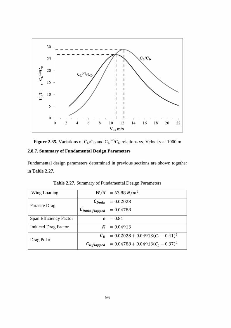
56
Figure 2.35. Variations of CL/CD and CL3/2
/CD relations vs. Velocity at 1000 m
2.8.7. Summary of Fundamental Design Parameters
Fundamental design parameters determined in previous sections are shown together
in Table 2.27.
Table 2.27. Summary of Fundamental Design Parameters
Wing Loading 𝑾 𝑺⁄ = 63.88 𝑁/𝑚2
Parasite Drag 𝑪𝑫𝒎𝒊𝒏
𝑪𝑫𝒎𝒊𝒏,𝒇𝒍𝒂𝒑𝒑𝒆𝒅
= 0.02028
= 0.04788
Span Efficiency Factor 𝒆 = 0.81
Induced Drag Factor 𝑲 = 0.04913
Drag Polar 𝑪𝑫
𝑪𝑫,𝒇𝒍𝒂𝒑𝒑𝒆𝒅
= 0.02028 + 0.04913(𝐶𝐿 − 0.41)2
= 0.04788 + 0.04913(𝐶𝐿 − 0.37)2

57
2.9. Constraint Analysis (W/S vs. PA/W)
Constraint analysis allows identifying solution space for the airplane design. Wing
loading (W/S), Thrust to Weight ratio (T/W) and Power to Weight ratio (P/W) are
important design parameters and most of the aircraft performance equation can be
expressed in terms of these parameters. However, for a propeller driven aircraft, P/W
and T/W parameters are not meaningful without flight velocity and corresponding
propeller efficiency. Equation (2.51) gives the power and power available
expressions.
𝑃 = 𝑇𝑉∞, 𝑃𝐴 = 𝜂𝑝𝑟𝑃 (2.51)
where
𝑃 =𝑃𝐴𝜂𝑝𝑟
=𝑇𝐴𝑉∞𝜂𝑝𝑟
(2.52)
Propeller efficiency 𝜂𝑝𝑟varies with flight velocity and altitude for fixed pitch
propeller, thus PA/W term is more meaningful instead of P/W or T/W parameters
used in constraint analysis of a fixed pitch propeller driven aircraft since propeller
efficiency is already included in power available term as a variable.
Initial design requirements and additional performance requirements are taken into
account and presented in Table 2.28. Stall speed and maximum speed constraints are
general design requirements. 0.5 m/s (or 100 ft/min) is the maximum rate of climb
speed for general aviation aircrafts but it is taken as 0.3 m/s for the study. Maximum
turn load is also calculated for 45° of bank angle, which is also specified for this
study.
Table 2.28. Constraint Analysis Requirements
Constraints
Stall Speed 𝑉𝑠𝑡𝑎𝑙𝑙 = 8 𝑚/𝑠 @1000m
Climb Speed at Maximum Climb Angle 𝑉𝜃,𝑚𝑎𝑥 = 𝑉𝑠𝑡𝑎𝑙𝑙@3000m
Maximum Rate of Climb 0.3 m/s @ 3000m
Maximum Speed 13.9 m/s @ MSL
Sustained Level Turn 𝑛,max 𝑡𝑢𝑟𝑛 = 1.41 @ 45° bank angle

58
Aircraft performance equations are referenced from Anderson [15] and Raymer [18].
Derivations of the constraint equations are given in Appendix D.
2.9.1. Stall Speed Constraint
Stall speed constraint is the hand launch requirement. Aircraft should survive at
minimum 8 m/s throw speed at 1000 m as a design requirement. Stall speed
constraint is given in Section 2.5.4.
(𝑊 𝑆⁄ )𝑠𝑡𝑎𝑙𝑙 = 64.034 𝑁/𝑚2
2.9.2. Climb Speed Constraint
Climb speed is the other hand launch requirement. Aircraft should climb at stall
speed at 3000 m altitude with maximum climb angle which also constraints the throw
velocity and throw angle.
𝑉𝜃𝑚𝑎𝑥 = 𝑉𝑠𝑡𝑎𝑙𝑙
𝑃𝐴𝑊=4𝐾(𝑊/𝑆)
𝜌∞𝑉𝑠𝑡𝑎𝑙𝑙−(𝑉𝑠𝑡𝑎𝑙𝑙)
3𝜌∞𝐶𝐷,0(𝑊/𝑆)
(2.53)
2.9.3. Maximum Rate of Climb Constraint
Maximum rate of climb constraint is the service ceiling requirement which is 0.3 m/s
at 3000 m altitude. For simplicity, maximum rate of climb equation for aircraft with
symmetrical airfoil is preferred for the constraint analysis.
𝑃𝐴𝑊= (
𝑅
𝐶)𝑚𝑎𝑥
+(2
𝜌∞
𝑊
𝑆(√3𝐶𝐷0𝐾
+ 4𝐶𝐿,𝐷𝑚𝑖𝑛2 − 𝐶𝐿,𝐷𝑚𝑖𝑛)
−1
)
1/2
×1.155
√1
4𝐾𝐶𝐷0+ (
𝐶𝐿,𝐷𝑚𝑖𝑛
2𝐶𝐷0)2
+𝐶𝐿,𝐷𝑚𝑖𝑛
2𝐶𝐷0
(2.54)

59
2.9.4. Maximum Speed Constraint
Maximum speed constraint is not a fundamental requirement since the maximum
velocity of the aircraft is limited. Even so, power required to achieve the cruise speed
at sea level should be defined. Sea level is the determinant condition for maximum
speed since air density and drag is higher.
𝑃𝐴𝑊= √
2
𝜌0(𝐶𝐷0 +𝐾(
(𝑊
𝑆)
1
2𝜌0𝑉𝑚𝑎𝑥2
− 𝐶𝐿,𝐷𝑚𝑖𝑛)
2
)((1
2𝜌0𝑉𝑚𝑎𝑥
2 )3/2
(𝑊/𝑆)) (2.55)
2.9.5. Sustained Level Turn Constraint
In the present study, maneuverability of the aircraft is not the preliminary
requirement. Sustained turn is constrained to maximum 45 degree bank angle, which
corresponds to 1.41 g turn. Sustained level turn constraint becomes dominant at
higher bank angles which is not preferred. Sustained level turn is constrained by the
thrust available or power available at a specified flight speed, and given as,
(𝑃𝐴𝑊) =
1
2𝜌∞𝑉∞
3𝐶𝐷0(𝑊 𝑆⁄ )
+𝑛2𝐾(𝑊 𝑆⁄ )1
2𝜌∞𝑉∞
(2.56)
2.9.6. Constraint Diagram and PA/W Requirement
Determined constraint equations are plotted in Figure 2.36. Design points for empty
weight (W0) condition to MTOW are indicated with the red dots. Since portability
requirement is also considered for constant MTOW constraint, which leads to
minimum size design, minimum wing area and highest possible wing loading point is
selected as shown in the Figure 2.36. Unfortunately power available is not constant
due to propeller efficiency variation with speed as mentioned. Therefore, design
points indicated in the constraint diagram are not actual design points but give an
idea about power requirement at a specific condition. Dominant performance
constraint is the maximum rate of climb requirement at 3000 m altitude, where
maximum power available is needed to achieve maximum rate of climb. Therefore
𝑷𝑨 𝑾⁄ = 𝟏.𝟕 is point is selected as an appropriate design value to estimate
propulsion requirements.

60
Figure 2.36. Constraint Diagram for PA/W
2.9.7. Thrust Requirement at the Design Point
Thrust at maximum rate of climb requirement is estimated from power available
requirement at maximum rate of climb velocity at 3000 m.
𝑃𝐴𝑊=𝑇
𝑊⋅ 𝑉(𝑅/𝐶)𝑚𝑎𝑥@3000𝑚
1.7 =𝑇
(39.24 𝑁)(12.0 𝑚/𝑠)
Thrust requirement to sustain maximum rate of climb at 3000 m is determined as.
𝑇 = 5.6 𝑁 = 0.57 𝑘𝑔𝑓 (@ 12𝑚 𝑠⁄ ,@3000𝑚).
Selected propulsion system should provide estimated thrust requirement at the design
point and thrust estimation should be checked after dynamic thrust calculations.

61
2.10. Dynamic Thrust Estimation
Dynamic thrust estimation of a fixed pitch propeller – electric motor system is very
important to determine reliable aircraft performance results. In this section, electric
motor and fixed pitch propeller combination is chosen and dynamic thrust results of
the propulsion system is determined by wind tunnel experiment. Results are used to
determine and validate dynamic thrust estimation model presented in the study in
order to estimate high altitude thrust and power available.
Dynamic thrust of a propeller decreases with increasing velocity since relative angle
of attack decreases due to increasing forward flight velocity component. Therefore,
propeller efficiency 𝜂𝑝𝑟 varies with velocity, which is maximized at the best design
speed - RPM ratio (V/n). In more detail, propeller efficiency 𝜂𝑝𝑟 is expressed as a
function of the advance ratio (J) which includes freestream velocity (𝑉∞), propeller
revolution per second (rps) (N) and propeller diameter (D). Advance ratio is given by
Eqn. (2.57) and Figure 2.37 shows the variation of the propeller efficiency with
respect to the advance ratio for various pitch angles.
𝐽 =𝑉∞𝑁𝐷
(2.57)
Figure 2.37. Propeller Efficiency vs. Advance Ratio for Various Pitch Angles [20]
As can be seen from Figure 2.37, propeller efficiency can be maximized by
changing the blade angle for variable-pitch propellers. However, maximum propeller
efficiency, corresponding advance ratio and consequently flight velocity varies for

62
different fixed-pitch propellers. Therefore, propeller efficiency cannot be assumed as
a constant for fixed-pitch propellers.
It should be noted that, propeller efficiency is also related with aerodynamic
characteristics, i.e. lift and drag coefficients of the airfoil used in the propeller blade
which is related with Reynolds number. Lift and drag coefficients decrease with
decreasing Reynolds number for increasing altitude due to air density and viscosity
change. Therefore, propeller efficiency is also decrease and propeller pitch should be
increased with altitude in order to maintain best efficiency. Thus, propellers with
different pitch should be used for different operation altitudes. However, only
performance variation of the selected propeller is determined for aircraft
performance calculations. Since maximum speed requirement is not the primary
requirement, low-pitch propeller and proper electric motor is chosen for the design.
Propellers with different pitch or diameter are not studied in this work.
2.10.1. Electric Motor and Propeller Selection
Propeller thrust gradually decreases and propeller efficiency changes with forward
flight velocity. Additionally, maximum forward velocity achievable which is called
as pitch speed is different for each propeller having different pitch. Therefore
selecting the propeller-motor combination is performed by trial and error. Selecting
the propulsion system requires some experience on drive systems.
Literature research and numerical experiments on propeller and drive system
calculators is performed and EMAX – GT 2218/11 motor is chosen for the low
energy consumption and sufficient thrust generation with the recommended propeller
[22], [23], [24]. Figure 2.38 shows the selected EMAX – GT2218/11 brushless out-
runner motor.
Figure 2.38. EMAX – GT2218/11 Brushless Out-Runner Motor

63
Performance data of the selected motor with the recommended propellers is given in
Table 2.29 [22].
Table 2.29. EMAX – GT2218/11 Performance with Recommended Propellers [22]
Model Cell
Count RPM/V
Prop
(APC) RPM
Max
Current
(<60S)
Thrust
GT2218/11 3S 930 11x4.7 7000 17A 1120 gr
3S 930 12x6 6700 18A 1150 gr
Based on the data provided in Table 2.29, APC – Slow Flyer – 11x4.7 propeller is
chosen for low maximum current requirement. Experimental propeller performance
data is taken from reference [21] and given in Appendix E. Maximum propeller
efficiency 𝜂𝑝𝑟 , 𝑚𝑎𝑥 is given as 0.648. Selected propeller and propeller efficiency
versus advance ratio plot at different RPMs are shown in Figure 2.39.
Figure 2.39. APC Slow Flyer 11x4.7 Propeller and 𝜂𝑝𝑟 vs. J plot

64
2.10.2. Dynamic Thrust Experiment
In order to determine the performance of the motor-propeller combination and verify
dynamic thrust model explained in following section, dynamic thrust experiment is
conducted in a low speed, continuous flow blower type wind tunnel located in
METU Aerospace Engineering Department Hangar Facilities which is shown in
Figure 2.40.
Figure 2.40. METU Aerospace Engineering Dept. Low Speed Wind Tunnel
Motor is mounted on a 6-axis load cell (ATI F/T Sensor: Gamma [25]) in order to
measure the thrust force and the propeller torque. Load cell power is supplied by DC
– Power supply and data is gathered by the National Instruments, NI-USB-6211 data
acquisition system and LabVIEW Software specialized by ATI Sensors [26]. Setup
components are given and identified by letters in Table 2.30.
Table 2.30. Experimental Setup Components
A APC – Slow Flyer – 11x4.7 Propeller F 40 A - ESC
B EMAX – GT2218/11 Motor G DC – Power Supply (11.1 V)
C ATI F/T Sensor: Gamma Load Cell H Computer
D RPM Sensor I 2.4 GHz Transmitter
E Test Mount J 2.4 GHz Receiver

65
Experimental setup components are shown in Figure 2.41 and Figure 2.42 shows
the experimental setup placed in the wind tunnel.
Figure 2.41. Experimental Setup
Figure 2.42. Experimental Setup Placed in the Wind Tunnel
Dynamic thrust experiment is performed for flow speeds ranging from 2.2 m/s to
17.6 m/s at the maximum throttle condition and at 930m (AMSL) altitude. Static
thrust (V=0) test is performed before the wind tunnel experiment and results are
presented in the dynamic thrust result table given in Table 2.31. Thrust and torque
data are gathered from load cell measurements. Power, power available and propeller
efficiency data are calculated from,
𝑃 = 2𝜋 ⋅ 𝑛 ⋅ 𝑄, 𝑃𝐴 = 𝑇 ⋅ 𝑉, 𝜂𝑝𝑟 = 𝑃𝐴/𝑃 (2.58)

66
Table 2.31. Experimental and Calculated Results
Experimental Results Calculated Results
V
(m/s)
T
(N)
Q
(N.m)
n
(RPM)
I
(Amp)
P
(Watt)
PA
(Watt)
𝜼𝒑𝒓
Static 0 9.891 0.164 6970 15.80
120.00 0 0
Dyn
am
ic T
hru
st
2.22 9.142 0.158 6972 15.13
115.43 20.30 0.176
3.09 8.785 0.156 6977 14.80
113.69 27.14 0.239
5.51 7.729 0.148 7003 14.23
108.75 42.58 0.392
7.75 6.745 0.143 7055 13.80
105.94 52.27 0.493
9.94 5.756 0.138 7152 13.30
103.06 57.21 0.555
11.83 4.798 0.131 7281 12.70
100.11 56.76 0.567
13.60 3.888 0.125 7419 12.14
96.73 52.88 0.547
15.00 3.031 0.119 7553 11.64
93.81 45.46 0.485
16.15 2.288 0.114 7669 11.20
91.63 36.95 0.403
17.07 1.724 0.111 7755 10.88
89.98 29.42 0.327
Measured dynamic thrust and calculated power available data with respect to
velocity are given together in Figure 2.43. As mentioned, power available varies
with velocity. Propeller efficiency is calculated from dynamic thrust and power
available data and shown in Figure 2.44. As expected, maximum propeller
efficiency is smaller than reference data which is obtained at lower altitude [21].
Measured RPM, shaft power and current plots are given in Figure 2.45, Figure 2.46
and Figure 2.47 respectively. According to the experimental results, maximum shaft
power is 120 W, maximum static thrust is 9.89 N and maximum draining current is
15.8 Amp which approximately matches with the manufacturer data given in Table
2.29.
Figure 2.43. Dynamic Thrust and Power Available vs. Velocity
PA
T

67
Figure 2.44. Propeller Efficiency vs. Velocity
Figure 2.45. Propeller RPM vs. Velocity
Figure 2.46. Shaft Power vs. Velocity

68
Figure 2.47. Draining Current vs. Velocity
RPM vs. shaft power and RPM vs. draining current relations can also be determined
from experimental results. However, dynamic thrust estimation model given in the
following section is only focused on the dynamic thrust and power available
variation with respect to flight velocity. Therefore it should be noted that actual RPM
value is not decisive in the model but increment of the RPM is considered in
calculations.
2.10.3. Dynamic Thrust Estimation Model
In this section, dynamic thrust estimation model is presented as a contribution of the
study. As mentioned, presented model is focused on the dynamic thrust and power
available results calculated from propeller performance data which can be
determined from manufacturer or an experimental study. In this study experimental
propeller performance data is used [21] and standard definitions of propeller
aerodynamic coefficients given in Eqn. (2.59) [27] are used to determine dynamic
thrust and power available results.
𝐽 =𝑉
𝑛𝐷, 𝐶𝑇 =
𝑇
𝜌𝑛2𝐷4, 𝐶𝑃 =
𝑃
𝜌𝑛3𝐷5, 𝜂𝑝𝑟 =
𝑇𝑉
𝑃=𝐶𝑇𝐽
𝐶𝑃 (2.59)
Main point of the model is utilizing the propeller performance data in order to
calculate reference altitude (sea level) results and adding power correction factor
(PcF) and altitude correction factors (AF) for high altitude calculations. Since
performance data of the propeller obtained from reference [21] is low altitude

69
experimental data, dynamic thrust calculations performed for higher altitudes are
needed to be corrected by using these correction factors.
Experimental propeller performance data is taken from [21] and first 5 rows of the
data are given in Table 2.32. Complete data table is provided in Appendix E.
Advance ratio vs. propeller efficiency plot of the performance data was given in
Figure 2.39.
Table 2.32. APC-SF-11x4.7, Experimental Performance Data [21]
J CT CP 𝜼𝒑𝒓
0.087 0.1151 0.0482 0.209
0.107 0.112 0.0477 0.250
0.133 0.1071 0.0468 0.305
0.155 0.1033 0.0461 0.346
0.175 0.0996 0.0454 0.385
... ... ... ...
Determination of the dynamic thrust with respect to altitude involves multi-variable
and coupled relations. Propeller efficiency 𝜼𝒑𝒓 is determined from the thrust
generated and power available at any speed. Thrust and aerodynamic power of the
propeller are also related to the propeller revolution and the diameter. Although
propeller diameter is constant, propeller RPM varies with the density and with the
forward flight velocity due to the variation of the aerodynamic torque. Electric motor
efficiency also varies with the number of revolution, draining current, operating
temperature, battery voltage and discharge rate. There are many dependent variables
to obtain a direct analytical relation of dynamic thrust for various altitudes, and this
is not within the scope of the thesis. Detailed experimental studies at various
altitudes are suggested to investigate propulsive efficiency of the motor and the
fixed-pitch propeller combinations for the maximum throttle condition. In the present
study, dynamic thrust calculation for fixed-pitch propeller is performed for the
reference altitude and an approximation method is presented to estimate dynamic
thrust results for higher altitudes.

70
Propeller aerodynamic coefficients given in Eqn. (2.59) are rewritten as follows,
𝑛𝐷 =𝑉
𝐽, 𝐶𝑇 =
𝑇
𝜌(𝑛𝐷)2𝐷2, 𝐶𝑃 =
𝑃
𝜌(𝑛𝐷)3𝐷2 (2.60)
From the power coefficient (𝑪𝑷) expression,
𝑃 = 𝐶𝑃𝜌(𝑛𝐷)3𝐷2
𝑃 = 𝐶𝑃𝜌 (𝑉
𝐽)3
𝐷2 (2.61)
where P is the maximum mechanical power (shaft power) generated by the electric
motor. As can be seen from RPM vs. Velocity plot and Shaft Power vs. Velocity plot
given in Figure 2.45 and Figure 2.46, shaft power decreases with RPM. In order to
represent the shaft power decrease of the electric motor due to RPM increase,
relation between RPM and shaft power is expressed with a power correction factor
(PcF).
As a starting point, maximum power is assumed constant as 120 W. Hence, initial
estimation for forward flight velocities at the reference altitude can be determined for
each 𝐽 − 𝐶𝑃 data given in Table 2.32.Eqn. (2.61) can be solved for velocity as,
𝑉𝑖𝑛𝑖𝑡 = (𝑃0𝐽
3
𝐶𝑃𝜌𝐷2)
1/3
(2.62)
By substituting Eqn. (2.62) into the advance ratio equation, initial estimation of the
propeller rps is calculated for each of the initial flight velocity at the reference
altitude.
𝑛𝑖𝑛𝑖𝑡 =(𝑃0𝐽
3
𝐶𝑃𝜌𝐷2)1/3
𝐽𝐷 (2.63)
Corrected dynamic shaft power can be calculated using the initial number of
revolution ratio and hypothetical Power correction Factor (PcF), which can be taken
as a number around 3, since power is related to the third power of the propeller rps.
In the present study, Eqn. (2.64) is proposed as the corrected dynamic shaft power
relation.

71
Calculation results are given in Table 2.33 and Figure 2.48 for PcF=2.7 value for
the selected motor – propeller combination which is determined by trial and error for
this study.
𝑃𝑐 = 𝑃0 (𝑛0𝑛)𝑷𝒄𝑭
(2.64)
Table 2.33. Corrected Shaft Power Calculations
Po V,init n,init Pc
120 2.58 106.08 (n0) 120.00
120 3.18 106.45 118.88
120 3.98 107.12 116.86
120 4.66 107.66 115.28
120 5.29 108.21 113.71
120 5.98 108.70 112.35
... ... ... ...
Figure 2.48. Constant and Corrected Shaft Power vs. Velocity
PcF adjusts shaft power at higher flight speeds where rotational speed of the
propeller is increased due to propeller torque decrease. By this way, pitch speed of
the propeller is decreased. Graphically, PcF has a rotation effect on the dynamic
thrust curve in clockwise direction as shown in Figure 2.49.

72
Figure 2.49. Effect of Power Correction Factor on Shaft Power
By using the corrected shaft power, forward flight velocity and propeller rps can be
calculated as follows.
𝑉 = (𝑃𝑐𝐽
3
𝐶𝑃𝜌𝐷2)
1/3
(2.65)
𝑛 =(𝑃𝑐𝐽
3
𝐶𝑃𝜌𝐷2)1/3
𝐽𝐷 (2.66)
From the thrust coefficient relation (𝑪𝑻) given by Eqn. (2.59), dynamic thrust can be
calculated for each flight velocity and corresponding rotational speed as,
𝑇 = 𝐶𝑇𝜌𝑛2𝐷4 (2.67)
As given in Eqn.(2.67), thrust is directly proportional to the air density for constant
rotational speed. However, at higher altitudes, rotational speed of the propeller
increases due to the torque decrement of the propeller since Reynolds number and
consequently drag coefficient of the propeller decreases with increasing altitude. As
a result thrust generated is amplified and propulsive efficiency is also affected due to
the change in the rotational speed of the motor, as mentioned before. In order to
estimate the dynamic thrust generated at high altitude, density ratio between the

73
target altitude and the reference altitude should be used by taking the thrust
amplification into account.
In the present study, another hypothetical parameter “Altitude Factor for Propulsive
Efficiency (𝑨𝑭𝜼)” is proposed to estimate the thrust ratio between the target altitude
and the reference altitude. Altitude Factor for Propulsive Efficiency is defined by
Eqns. (2.68) and (2.69) and it is given by the air density ratio raised to power AF
which is less than 1.
𝑇
𝑇0=𝑃𝐴𝑃𝐴,0
= (𝜌
𝜌0)𝑨𝑭
(2.68)
𝐴𝐹𝜂 = (𝜌
𝜌0)𝑨𝑭
(2.69)
As can be seen from Eqn. (2.68), altitude factor 𝐴𝐹𝜂 is analogous with the altitude
variation approximation for turboprop engines for which propulsive power is mainly
generated by the propeller [15]. “AF” factor can be related with diameter, pitch angle
of the propeller and airfoil characteristics of the propeller blade which are directly
related with the propeller performance.
Up to this point, definitions and effects of the correction factors are given. Complete
model of the dynamic thrust estimation model proposed in the study is shown in
Figure 2.50. Firstly corrected dynamic thrust and power available calculations are
performed for the reference altitude and then higher altitude results are determined
by using the Altitude Factor.
Figure 2.50. Dynamic Thrust Estimation Model
𝑃0 𝑉𝑖𝑛𝑖𝑡
𝑛𝑖𝑛𝑖𝑡
𝑃𝐶 𝑇𝐴,0 𝑃𝐴,0 𝑉
𝑛
𝑃𝐶𝑃0= (
𝑛0𝑛)𝑃𝑐𝐹
𝑇𝐴𝑇𝐴,0
=𝑃𝐴𝑃𝐴,0
= (𝜌
𝜌0)𝐴𝐹

74
As mentioned before, Power Correction Factor PcF and Thrust Amplification Factor
(Altitude Factor) AF parameters are hypothetical parameters, which are “Motor
Performance and Design Unknown” and “Propeller Performance and Design
Unknown”. Altitude Factor (AF) corrects maximum thrust value for higher altitudes
with respect to reference altitude and Power Correction Factor (PcF) corrects
maximum pitch speed value by reducing power at higher speeds (Eqn. (2.65)). Effect
of these correction parameters on thrust curve are shown in Figure 2.51.
Figure 2.51. Effects of AF and PcF parameters on Dynamic Thrust Curve
As can be seen from the dynamic thrust curves given in Figure 2.51, firstly AF and
PcF parameters are set to zero as a starting point, then AF parameter is applied for
maximum thrust correction and then PcF parameter is applied for maximum pitch
speed correction. Correction factor values are found by trial and error for the present
design. AF parameter is set to 0.8 and PcF parameter is set to 2.7 in order to meet the
estimated dynamic thrust and power available curves with experimental results
performed at 930 m (AMSL) altitude.

75
Final dynamic thrust and power available versus speed curves are shown in Figure
2.52 and Figure 2.53 respectively. Uncorrected results of thrust and power available
calculations are also shown for comparison. For uncorrected case PcF is set to 0 for
constant maximum power assumption as shown in Figure 2.49 and AF is set to 1 for
direct analytic solution calculated from Eqn.(2.67). As mentioned pitch speed
calculation is quite high and shaft power is not decreased with velocity and RPM
increase for uncorrected case. As a result, thrust available, power available and pitch
speed results are found illusively high for uncorrected calculations. However,
corrected results of the dynamic thrust estimation model fit with experimental results
almost perfectly.
Figure 2.52. Dynamic Thrust Model and Experimental Thrust Results
Figure 2.53. Power Available Curves of Experimental and Dynamic Thrust Model

76
2.10.4. Dynamic Thrust Variation with Altitude
Dynamic thrusts at different altitudes are calculated from Eqn. (2.70) and results are
presented in Figure 2.54.
𝑇𝐴 = 𝑇𝐴,0 ⋅ 𝐴𝐹𝜂 = 𝑇𝐴,0 ⋅ (𝜌
𝜌0)𝟎.𝟖
(2.70)
Figure 2.54. Dynamic Thrust at Various Altitudes
Increase behavior in RPM with velocity and altitude drives the dynamic thrust
estimation model. As mentioned before, actual RPM values are not interested at this
point but the behavior of the increment is. Firstly, RPM of the propeller at the
reference altitude is calculated from Eqn. (2.63) then rotational speeds at high
altitudes are obtained from Eqn. (2.67) by using the approximated dynamic thrust
values. Results are given in Figure 2.55.

77
Figure 2.55. Rotational Speed of the Propeller vs. Velocity at Various Altitudes
Power available and corresponding propeller efficiencies are also calculated using
the dynamic thrust approximations, as given in Eqn. (2.71). Propeller efficiencies,
given by Eqn. (2.72), are then used to determine “P/W” curves in the constraint
diagram at velocities specified in constraint analysis.
𝑃𝐴 = 𝜂𝑝𝑟𝑃 = 𝑇𝐴𝑉 (2.71)
𝜂𝑝𝑟 =𝑃𝐴𝑃
(2.72)
𝑃 =𝑃𝐴𝜂𝑝𝑟
(2.73)
Power available and propeller efficiency vs. velocity plots are given in Figure 2.56
and Figure 2.57 at various altitudes. These plots allow one to use more realistic
available power and propeller efficiency values which in reality change with the
altitude as opposed to using single power available and propeller efficiency curves
which what is commonly practiced.
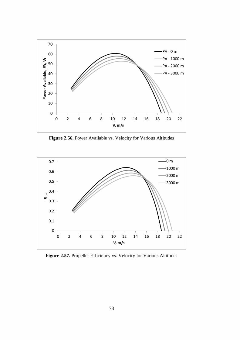
78
Figure 2.56. Power Available vs. Velocity for Various Altitudes
Figure 2.57. Propeller Efficiency vs. Velocity for Various Altitudes
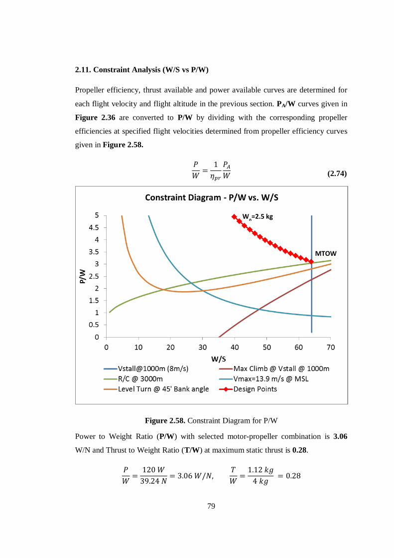
79
2.11. Constraint Analysis (W/S vs P/W)
Propeller efficiency, thrust available and power available curves are determined for
each flight velocity and flight altitude in the previous section. PA/W curves given in
Figure 2.36 are converted to P/W by dividing with the corresponding propeller
efficiencies at specified flight velocities determined from propeller efficiency curves
given in Figure 2.58.
𝑃
𝑊=1
𝜂𝑝𝑟
𝑃𝐴𝑊
(2.74)
Figure 2.58. Constraint Diagram for P/W
Power to Weight Ratio (P/W) with selected motor-propeller combination is 3.06
W/N and Thrust to Weight Ratio (T/W) at maximum static thrust is 0.28.
𝑃
𝑊=120 𝑊
39.24 𝑁= 3.06 𝑊/𝑁,
𝑇
𝑊=1.12 𝑘𝑔
4 𝑘𝑔 = 0.28
W0=2.5 kg
MTOW

80
2.12. Aircraft Performance Analysis
Aircraft performance analysis is performed by using the standard performance
equations referenced from Anderson [15] and Raymer [18].In classical performance
analysis of a propeller-driven aircraft, performance equations are derived for constant
power available assumption, where propeller efficiency is constant due to constant
speed – variable pitch propeller assumptions. However, for a fixed-pitch propeller
driven aircraft, such assumptions are not applicable since propeller efficiency varies
with speed and altitude. Thus, direct analytical approaches leads to incorrect results
and graphical approach is suggested to determine the performance parameters for a
fixed-pitch propeller driven aircraft.
2.12.1. Aircraft Performance Parameters (TR, PR, TA, PA) and Critical Velocities
Thrust required, which is equal to the drag of the aircraft, is calculated by,
𝑇𝑅 = 𝐷 =1
2𝜌∞𝑉∞
2𝑆𝐶𝐷 (2.75)
where drag coefficient which is given in Eqn. (2.37) is recalled.
𝐶𝐷 = 0.01457 + 0.04102(𝐶𝐿 − 0.43)2
Thrust available curves are determined in Section 2.10.3 by using Eqn. (2.70).
𝑇𝐴 = 𝑇𝐴,0 ⋅ 𝐴𝐹𝜂 = 𝑇𝐴,0 ⋅ (𝜌
𝜌0)𝟎.𝟖
Power required and power available are calculated by,
𝑃𝑅 = 𝑇𝑅𝑉∞ = 𝐷𝑉∞ (2.76)
𝑃𝐴 = 𝑇𝐴𝑉∞ (2.71)
Dynamic thrust and power curves for design altitude boundaries are shown in Figure
2.59 and Figure 2.60 with critical design velocities. As calculated before and
summarized in Table 2.26 in Section 2.8.6, cruise velocities are 11.7 m/s at sea level
and 13.6 m/s at 3000 m design altitudes where thrust required values are minimum.
Similarly, loiter speeds are 10.4 m/s at sea level and 12 m/s at 3000 m design
altitudes where power required values are minimum. Attainable maximum velocities
are 16.2 m/s and 17.6 m/s for sea level and 3000 m design altitudes, respectively.

81
Figure 2.59. Drag (TR) and Thrust Available Curves
Figure 2.60. Power Required and Power Available Curves
(
𝑉𝑙𝑜𝑖𝑡𝑒𝑟@ 0𝑚 = 10.4𝑚 𝑠⁄ , 𝑉𝑙𝑜𝑖𝑡𝑒𝑟@ 3000𝑚 = 12.0𝑚 𝑠⁄
𝑉𝑐𝑟𝑢𝑖𝑠𝑒@ 0𝑚 = 11.7𝑚 𝑠⁄ , 𝑉𝑐𝑟𝑢𝑖𝑠𝑒@ 3000𝑚 = 13.6𝑚 𝑠⁄
𝑉𝑚𝑎𝑥@ 0𝑚 = 16.2𝑚 𝑠⁄ , 𝑉𝑚𝑎𝑥@ 3000𝑚 = 17.6𝑚 𝑠⁄)
TR
TA
PA
PR
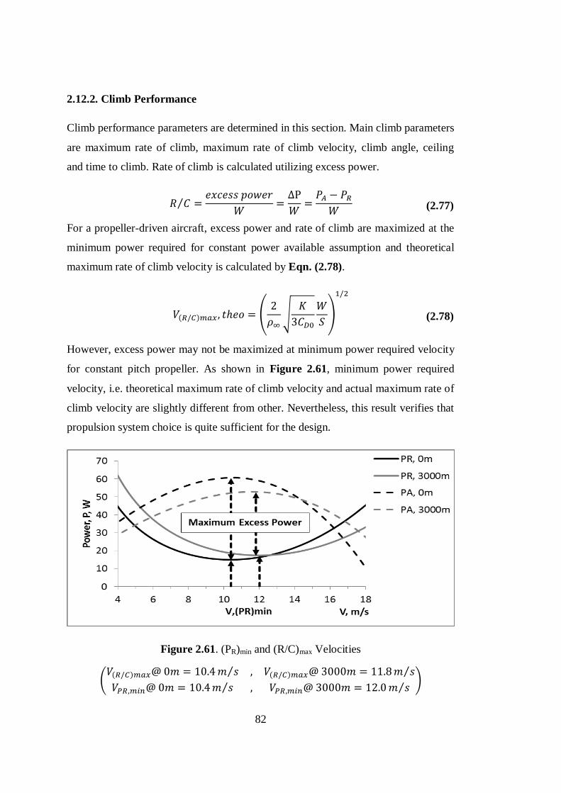
82
2.12.2. Climb Performance
Climb performance parameters are determined in this section. Main climb parameters
are maximum rate of climb, maximum rate of climb velocity, climb angle, ceiling
and time to climb. Rate of climb is calculated utilizing excess power.
𝑅 𝐶⁄ =𝑒𝑥𝑐𝑒𝑠𝑠 𝑝𝑜𝑤𝑒𝑟
𝑊=ΔP
𝑊=𝑃𝐴 − 𝑃𝑅𝑊
(2.77)
For a propeller-driven aircraft, excess power and rate of climb are maximized at the
minimum power required for constant power available assumption and theoretical
maximum rate of climb velocity is calculated by Eqn. (2.78).
𝑉(𝑅/𝐶)𝑚𝑎𝑥 , 𝑡ℎ𝑒𝑜 = (2
𝜌∞√𝐾
3𝐶𝐷0
𝑊
𝑆)
1/2
(2.78)
However, excess power may not be maximized at minimum power required velocity
for constant pitch propeller. As shown in Figure 2.61, minimum power required
velocity, i.e. theoretical maximum rate of climb velocity and actual maximum rate of
climb velocity are slightly different from other. Nevertheless, this result verifies that
propulsion system choice is quite sufficient for the design.
Figure 2.61. (PR)min and (R/C)max Velocities
(𝑉(𝑅/𝐶)𝑚𝑎𝑥@ 0𝑚 = 10.4𝑚 𝑠⁄ , 𝑉(𝑅/𝐶)𝑚𝑎𝑥@ 3000𝑚 = 11.8𝑚 𝑠⁄
𝑉𝑃𝑅,𝑚𝑖𝑛@ 0𝑚 = 10.4𝑚 𝑠⁄ , 𝑉𝑃𝑅,𝑚𝑖𝑛@ 3000𝑚 = 12.0𝑚 𝑠⁄)

83
Difference between theoretical and actual rate of climb velocities might be much
higher if different propeller were chosen. Therefore graphical approach is needed to
determine actual maximum rate of climb velocity for aircraft with constant pitch
propeller. Rate of climb variation with altitude are also calculated from excess power
values shown in Figure 2.61 and Eqn. (2.77).
Figure 2.62. Rate of Climb Variation with Altitude
Theoretical maximum rate of climb velocities and actual maximum rate of climb
velocities shown in Figure 2.62 are summarized in Table 2.34. As it is mentioned
before, closeness between theoretical and actual maximum rate of climb velocities
verifies the suitability of the propulsion system choice.
Table 2.34. Theoretical and Actual V(R/C)max Variation with Altitude
Altitude Theoretical
𝑽(𝑹 𝑪⁄ )𝒎𝒂𝒙 = 𝑽𝑷𝑹,𝒎𝒊𝒏
Actual
𝑽(𝑹/𝑪)𝒎𝒂𝒙
0 10.4 10.4
1000 10.9 10.9
2000 11.4 11.3
3000 12.0 11.8

84
2.12.2.1. Climb Angle
Climb angle for a propeller-driven aircraft can be directly calculated by Eqn. (2.79),
where 𝑉∞ is maximum rate of climb velocity and 𝑃𝐴 is the power available at
maximum rate of climb velocity.
sin 𝜃 =𝑃𝐴𝑉∞𝑊
−1
2𝜌∞𝑉∞
2 (𝑊
𝑆)−1
𝐶𝐷0 −𝑊
𝑆
2𝐾
𝜌∞𝑉∞2 (2.79)
Table 2.35. Climb Angles with Altitude
Altitude, m 0 1000 2000 3000 4000
𝜽, deg 5.1 4.3 3.5 2.8 2.1
Figure 2.63. Climb Angle with Altitude at Maximum Rate of Climb
2.12.2.2. Service and Absolute Ceiling
Service ceiling is the altitude where maximum rate of climb is 0.5 m/s (100 ft/min)
for general aviation aircraft[18], which is quite high for a Mini UAV. 0.3 m/s
maximum rate of climb is assumed for the design. Maximum rate of climb with
altitude has a linear trend which is shown in Figure 2.64.

85
Figure 2.64. Maximum Rate of Climb Trend
It is seen from the trend plot that, service and absolute ceiling values determined as
13000 m and 9750 m are not realistic. Ceiling calculations are performed based on
approximations shown in Section2.10.3 where altitude factor 𝐴𝐹𝜂 assumption is
assumed for limited altitude values and temperature effects on propulsion system are
not included. Nevertheless, rate of climb calculations may be assumed realistic in
design altitudes with a large safety margin. Additionally, mini UAV’s structures and
systems are not designed for very high altitude operations where air temperature and
pressure are extremely low. Therefore, operational ceiling is limited up-to 4000 m.
2.12.2.3. Time to climb
Minimum time to climb is calculated from maximum rate of climb, where (𝑅/𝐶)𝑚𝑎𝑥
equation can be approximated from maximum rate of climb trend shown in Figure
2.64.
(𝑅/𝐶)𝑚𝑎𝑥 = −0.00009ℎ + 1.16602 (2.80)
𝑡𝑚𝑖𝑛 = ∫𝑑ℎ
(𝑅 𝐶⁄ )𝑚𝑎𝑥
ℎ2
ℎ1
(2.81)
𝑡𝑚𝑖𝑛 = (11111.1 ⋅ ln (1.16602 − 0.00009 ⋅ ℎ1))
− (11111.1 ⋅ ln(1.16602− 0.00009 ⋅ ℎ2))
(2.82)
Minimum time to climb results are calculated and presented in Table 2.36.

86
Table 2.36. Time to Climb Table
h1
(Ground Level)
h2
(100 m AGL)
tmin
(min:sec)
0 100 1:26
1000 1100 1:33
2000 2100 1:42
3000 3100 1:52
0 3100 48:47
Average climb time is 1:40 min (100 sec) to climb 100 m AGL operation altitude
and 50 minutes is needed to climb 3000 m from sea level.
2.12.3. Gliding and Unpowered Hand Launch
Determination of gliding parameters of the aircraft is important for unpowered flight
phase due to the fact that hand launch of the mini UAV may be initialized unpowered
for safety considerations. Minimum glide angle is independent from the flight
altitude and determined as,
tan 𝜃𝑚𝑖𝑛 =
1
(𝐿/𝐷)𝑚𝑎𝑥=
1
√ 1
4𝐾𝐶𝐷0+ (
𝐶𝐿,𝐷𝑚𝑖𝑛
2𝐶𝐷0)2
+𝐶𝐿,𝐷𝑚𝑖𝑛
2𝐶𝐷0
(2.83)
Minimum glide angles for flapped and unflapped aircraft are calculated as given in
Table 2.37.
Table 2.37. Minimum Glide Angles
(𝑳 𝑫⁄ )𝒎𝒂𝒙 𝜽𝒎𝒊𝒏
(degrees)
Flapped 28.90 1.98
Unflapped 14.90 3.85

87
Gliding velocity at minimum glide angle is the (𝐿 𝐷⁄ )𝑚𝑎𝑥 velocity at any altitude.
𝑉𝑔𝑙𝑖𝑑𝑒 = 𝑉(𝐿 𝐷⁄ )𝑚𝑎𝑥 (2.84)
Rate of descent of the aircraft at equilibrium glide velocity is given by,
𝑉𝑉 = 𝑉(𝐿 𝐷⁄ )𝑚𝑎𝑥 ⋅ sin(𝜃𝑚𝑖𝑛) (2.85)
Equilibrium glide velocities and rate of descent of the aircraft for various altitudes
are calculated by using (𝐿 𝐷⁄ )𝑚𝑎𝑥 velocities and minimum glide angles given in
Table 2.37. Results are presented in Table 2.38 and Figure 2.65.
Table 2.38. Glide velocities, Minimum Glide Angles and Descent Rates
Flapped Unflapped
𝜽𝒎𝒊𝒏 = 𝟏. 𝟗𝟖° 𝜽𝒎𝒊𝒏 = 𝟑.𝟖𝟓°
Altitude, m 𝑽𝒈𝒍𝒊𝒅𝒆,𝒎/𝒔 𝑽𝑽 ,𝒎/𝒔 𝑽𝒈𝒍𝒊𝒅𝒆,𝒎/𝒔 𝑽𝑽 ,𝒎/𝒔
0 9.9 0.34 11.7 0.78
1000 10.4 0.36 12.3 0.82
2000 11.0 0.38 12.9 0.87
3000 11.5 0.40 13.6 0.91
Figure 2.65. Variation of Glide Velocities and Stall Velocities vs Altitude

88
2.12.4. Takeoff Distance
Takeoff distance is calculated considering simple ground roll approximation since
the primary design requirement is takeoff by hand-launch. Takeoff requirement is
chosen as 35 m as given in the Constraint Analysis section. By assuming that thrust
is much higher than the drag and the rolling friction, ground roll can be approximated
as,
𝑠𝑔 ≈1.21 ⋅ (𝑊/𝑆)
𝑔 ⋅ 𝜌∞ ⋅ (𝐶𝐿)𝑚𝑎𝑥 ⋅ (𝑇/𝑊) (2.86)
Thrust to Weight ratio is not constant for propeller driven aircraft. Thrust at takeoff is
calculated from lift off speed which is given by,
𝑉𝐿𝑂 = 1.1 𝑉𝑠𝑡𝑎𝑙𝑙 (2.87)
Lift off speeds are calculated from stall velocities at design altitudes and
corresponding thrust values are taken from the thrust data found in Section2.10.3. By
using the calculated T/W values, ground roll is calculated and given in Table 2.39.
Table 2.39. Takeoff Distances for Various Altitudes
Altitude (m) 𝑽𝑳𝑶(m/s) 𝑻𝑨 (N) T/W 𝒔𝒈 (m)
0 8.4 8.11 0.207 17.3
1000 8.8 7.49 0.191 20.6
2000 9.2 6.90 0.176 24.7
3000 9.7 6.33 0.161 29.8
2.12.5. Range and Endurance Calculations for Electric-Powered Aircraft
Range and endurance relations are well established for piston propeller and jet
aircraft, which are derived from the specific fuel consumption and the fuel weight
fraction. However, specific fuel consumption and fuel weight fraction are not
available in electric-powered electric aircraft. Instead of these parameters, battery
discharge rate, current draw and battery capacity are used for the range and the
endurance estimations of the electric-powered aircraft. High performance battery
types that are widely used in small aircraft like R/C airplanes and Mini UAV’s are

89
Nickel-Cadmium (Ni-CD), Nickel-Metal Hydride (Ni-MH) and Lithium-Polymer
(Li-Po). Because of high energy rates per battery weight, Li-Po battery type is chosen
for the present design.
Li-Po battery cells are packed in serial and parallel connections in order to increase
the battery voltage and the overall capacity. However it is not possible to use the
100% of the battery capacity due to design feature of the Li-Po batteries since cells
exponentially discharge below critical cell voltages and become unusable. From the
typical discharge curves for low discharge rate and high discharge rate batteries
given in Figure 2.66, it is seen that about 15% of the Li-Po battery capacity should
be remained unused to protect the battery life. In other words, 85% of the battery
capacity should be taken to into account for range and endurance calculations.
Figure 2.66. Typical Discharge Curves of Li-Po Batteries
Range and endurance calculations for electric-powered aircraft are performed by
referencing Traub’s work [28] for typical Li-Po battery parameters. In order to
determine the endurance for electric-powered aircraft, discharge time of the battery is
calculated by using Peukert’s Equation in terms of battery capacity, current draw and
discharge rate.
𝑡 =𝑅𝑡
𝑖𝑛(𝐶
𝑅𝑡)𝑛
(2.88)

90
Power required of the aircraft is provided by the battery pack,
𝑃𝑅 = 𝑃𝐵 = 𝑉𝑖 (2.89)
Substitution of the discharge current “i” in Eqn. (2.88) into Eqn. (2.89) yields,
𝑃𝑅 = 𝑉𝐶
𝑅𝑡(𝑅𝑡
𝑡)1/𝑛
(2.90)
where,
t : Discharge time in hours (h)
i : Discharge current in amperes (A)
V : Battery voltage in volts (V) V=11.1 V (3S Li-Po Battery)
C : Battery capacity in amp. hours (Ah)
Rt : Battery hour rating in hours (h) Rt=1 (Based on 1 hour discharge
for portable batteries )
n : Battery discharge rate n=1.3 for typical Li-Po Battery [28]
Power output of the battery is reduced by the useable capacity factor, thermal losses,
mechanical losses and aerodynamic losses due to propeller efficiency. Total
efficiency can be expressed as,
𝜂𝑡𝑜𝑡 = 𝜂𝑐𝑎𝑝𝑎𝑐𝑖𝑡𝑦 ⋅ 𝜂𝑡ℎ𝑒𝑟𝑚𝑎𝑙 ⋅ 𝜂𝑚𝑒𝑐ℎ𝑎𝑛𝑖𝑐𝑎𝑙 ⋅ 𝜂𝑝𝑟 (2.91)
Where useable capacity factor is 0.85, thermal and mechanical losses are assumed as
0.75 and propeller efficiencies are taken from the corresponding data given in Figure
2.57.
𝜂𝑡𝑜𝑡 = 0.85 ⋅ 0.752 ⋅ 𝜂𝑝𝑟 = 0.478 ⋅ 𝜂𝑝𝑟
Total efficiency is added into Eqn. (2.90)and time results in endurance equation for
electric-powered aircraft are calculated.
𝐸 = 𝑡 = 𝑅𝑡1−𝑛 (𝜂𝑡𝑜𝑡𝑉 ⋅ 𝐶
𝑃𝑅)𝑛
(2.92)
where endurance is in hours for any flight velocity and altitude. Note that power
required is in terms of flight velocity and air density. Endurance plot calculated for

91
various flight speeds and battery capacities is given in Figure 2.67 for 1000 m flight
altitude.
Figure 2.67. Effect of Battery Capacity on Endurance at 1000 m Altitude
6800 mAh battery capacity is sufficient for 90 minutes of endurance requirement
with 11.4 m/s flight velocity at 1000 m flight altitude. However, 8200 mAh battery
capacity is required to achieve endurance requirement at the maximum cruise
velocity and 3000 m flight altitude as shown in Figure 2.68. 8200 mAh battery
provides 129 minutes of maximum endurance at sea level and 90 minutes of
endurance at 3000 m flight altitude for fixed loitering speed.Table 2.40 summarizes
maximum endurances and corresponding velocities at various altitudes.
Figure 2.68. Endurance vs Flight Velocity at Various Altitudes

92
Table 2.40. Maximum Endurance and Corresponding Velocities at Various Altitudes
Altitude
(m)
𝑽𝑳𝒐𝒊𝒕𝒆𝒓 (m/s)
𝑽𝑬,𝒎𝒂𝒙
(m/s)
E,max
(min)
0 10.4 11.3 129.0
1000 10.9 11.5 115.0
2000 11.4 12.7 102.3
3000 12.0 12.9 90.6
From Table 2.40, it is seen that maximum endurance of the aircraft is 129 minutes at
level and 90 minutes at 3000 m with the determined maximum endurance velocities.
Since theoretical loiter velocities and maximum endurance velocities are not
identical because of fixed pitch propeller efficiency change, calculated maximum
endurance velocities are determined as the actual loiter velocities. This results shows
that theoretical loiter speed is not reliable for fixed-pitch propeller aircrafts.
Range of the aircraft is simply calculated by multiplying flight time and flight
velocity shown in Figure 2.68 and Figure 2.69. Table 2.41 summarizes maximum
ranges and corresponding velocities at various design altitudes.
𝑅 = 𝐸 ⋅ 𝑉∞ (2.93)
Figure 2.69. Range vs Flight Velocity for Various Altitudes

93
Table 2.41. Maximum Ranges and Corresponding Velocities at Different Altitudes
Altitude
(m)
𝑽𝑪𝒓𝒖𝒊𝒔𝒆 (m/s)
𝐕𝐑,𝐦𝐚𝐱 (m/s)
R,max
(km)
0 11.7 11.7 87.1
1000 12.3 12.2 81.3
2000 12.9 12.8 75.7
3000 13.6 13.4 70.2
From Table 2.41, it is seen that maximum range of the aircraft is 87 km at sea level
and 70 km at 3000 m with the determined maximum range velocities and cruise
velocities determined by the graphical approach are quite close to calculated
maximum range velocities. Hence, cruise speeds and maximum range speed are
practically identical as expected. Calculated ranges are total distances covered
through mission time for fixed cruise speed at design altitudes. Actual battery
capacity requirement is determined by taking mission profile into account by
utilizing the calculated takeoff speed, climb speed, loitering and cruise speed
determined in the previous sections.
Mission profile of the aircraft was introduced in Section 2.3.1 and simple mission
profile was given in Figure 2.1 is referenced for the calculations. Design velocities at
each mission phase are determined as given in Table 2.42.
Table 2.42. Critical Design Speeds
Phase Phase Velocity 0 m 1000 m 2000 m 3000 m
Takeoff 𝑽𝒕𝒂𝒌𝒆𝒐𝒇𝒇 = 𝟏. 𝟏 ⋅ 𝑽𝒔𝒕𝒂𝒍𝒍 8.4 m/s 8.8 m/s 9.2 m/s 9.7 m/s
Climb 𝑽𝒄𝒍𝒊𝒎𝒃 = 𝑽(𝑹/𝑪)𝒎𝒂𝒙 10.4 m/s 10.9 m/s 11.3 m/s 11.8 m/s
Loiter 𝑽𝒍𝒐𝒊𝒕𝒆𝒓 = 𝑽𝑬,𝒎𝒂𝒙 11.3 m/s 11.5 m/s 12.7 m/s 12.9 m/s
Cruise 𝑽𝒄𝒓𝒖𝒊𝒔𝒆 = 𝑽𝑹,𝒎𝒂𝒙 11.7 m/s 12.2 m/s 12.8 m/s 13.4 m/s
Descend 𝑽𝒅𝒆𝒔𝒄𝒆𝒏𝒅 = 𝑽𝒈𝒍𝒊𝒅𝒆 11.7 m/s 12.3 m/s 12.9 m/s 13.6 m/s
Actual battery capacity requirement is determined by using Eqn. (2.92). Required
battery capacity at each mission phase is calculated as,
𝐶𝑝ℎ𝑎𝑠𝑒 =𝑃𝑅𝜂𝑡𝑜𝑡𝑉
(𝑅𝑡)𝑛−1
𝑛 (𝑡)1/𝑛 (2.94)

94
Power requirement at the take off and climb phases is 𝑃𝐴,𝑚𝑎𝑥 and for the rest of the
mission phases at the corresponding flight velocities and flight altitudes, calculated
power required values are used. Note that, power available varies with velocity and
altitude for fixed pitch propeller as mentioned before. Elapsed time and distances
covered during the mission time are calculated and given in Table 2.43 for 1000 m
operational altitude.
Table 2.43. Mission Profile and Required Battery Capacity
Stations Phase
Flight
Velocity
(m/s)
Elapsed
Time
(min:sec)
Distance
Covered
(km)
Required
Battery
Capacity
(mAh)
0 Take-off 8.8 00:05 0.021 130
0 – 1 Climb 10.9 01:33 1.01 1190
1 – 2 Cruise
(10 km) 12.2 13:40 10.0 1745
2 – 3 Loitering 11.5 59:40 41.2 5290
3 – 4
Return
Cruise
(10 km)
12.2 13:40 10.0 1745
4 – 5 Descend 12.3 01:22 1.01 300
5 Landing 8.8 - - -
Mission
Time
Total
Distance
Total
Capacity
90 min 63.2 km 10400 mAh
Similarly, mission time, total distance covered and total battery capacity requirement
are calculated for each design altitude and given in Table 2.44.
Table 2.44. Total Battery Capacity Requirement at Design Altitudes
Altitude Mission Time Total Distance Total Capacity
0 m 90 min 61.6 km 9600 mAh
1000 m 90 min 63.2 km 10400 mAh
2000 m 90 min 68.4 km 11500 mAh
3000 m 90 min 70.1 km 12400 mAh

95
According to Table 2.44, required battery capacity is 12400 mAh for the main
battery at 3000 m design altitude. Auxiliary battery is also needed to supply the
power requirement of the mission compartment and avionics of the aircraft.
Therefore 3 packs of parallel connected 5100 mAh 3S1P Li-Po battery (3S3P) is
used for the design [29].
Figure 2.70. Iris+ 5100 mAh 3S1P Li-Po Battery [29]
Total battery capacity is 15300 mAh and output voltage is 11.1V for selected 3S3P
battery pack. If needed, main battery capacity, in other words weight of the main
battery, may be decreased to ensure MTOW is not exceeded, which also reduces
mission time.
2.13. V-n Diagram
Structural limitations of the aircraft are defined in this section. Since Demircan Mini
UAV is not an aerobatic aircraft, limit loads are kept as small as possible. In order to
determine limit flight loads, firstly loads at sustained level turn are determined and
bending moment load for wing tip test is determined since wing tip test is necessary
and practical way to ensure the structural reliability of the wing structure. Finally,
limit load is defined considering the higher load factor.

96
2.13.1. Load at Sustained Level Turn
Sustained level turn is constrained by the maximum thrust available at any flight
speed where thrust available varies with the velocity for the propeller driven airplane.
Load factor at sustained level turn is calculated as,
𝑛 = 1 cos𝜙⁄ (2.95)
where maximum load factor “𝒏𝒎𝒂𝒙” was chosen as 1.41 for 𝟒𝟓° bank angle in
constraint analysis as a requirement. In this section, maximum load factor and
sustained level turn performance of the aircraft is calculated for the selected
propulsion system. Load factor in terms of (T/W) and flight performance parameters
is defined as,
𝑛 = {
1
2𝜌∞𝑉∞
2
𝐾(𝑊 𝑆⁄ )[𝑇
𝑊−1
2𝜌∞𝑉∞
2𝐶𝐷0𝑊/𝑆
]}
1/2
(2.96)
where (T/W) varies with the velocity. Maximum thrust available of a propeller is the
static thrust at zero velocity. Therefore, we cannot simply assume that load factor is
maximized at (T/W)max. Graphical solution methodology is needed to determine
maximum load factor at the sustained level turn for a propeller driven airplane.
Load factors are calculated for different altitudes by using the flight velocities and
the corresponding thrust available values determined in Section2.10.3. Load factor
results calculated from Eqn. (2.96) are plotted for design altitudes in Figure 2.71.

97
Figure 2.71. Thrust Constraint on Load Factor for Various Altitudes
Maximum turn load is obtained at sea level, where 𝒏𝒎𝒂𝒙,𝒕𝒖𝒓𝒏 = 𝟏. 𝟔𝟔 at 11.4 m/s.
Maximum achievable level flight (n=1) velocity is 16.2 m/s at 3000 m altitude and
maximum flight velocity is 17.6 m/s at 3000 m altitude with n=0.28 which shows
that aircraft cannot sustain level flight and should dive with 73.4° dive angle. This
dive velocity is also determined from intersection of drag and thrust available curves
and above this dive speed, aircraft drag overcomes the available thrust as shown in
Figure 2.59.
Figure 2.59.Drag (TR) and Thrust Available Curves vs Velocity

98
Turn radius for any flight velocity and load factor is calculated as;
𝑅 =𝑉∞2
𝑔√𝑛2 − 1 (2.97)
Maximum load factors, bank angles and turn radii at corresponding flight velocities
for various altitudes are given in Table 2.45.
Table 2.45. nmax, Bank Angles, Turn Radii for Various Altitudes
Altitude (m) 𝑽∞(m/s) n,max 𝝓 (deg) R (m)
0 11.4 1.66 53.0 10.0
1000 11.7 1.57 50.4 11.6
2000 12.0 1.47 47.2 13.6
3000 12.3 1.38 43.6 16.2
Maximum lift coefficient also constraints maximum load factor which is practically
the stall constraint with the load factor, where 𝐶𝐿,𝑚𝑎𝑥 is 1.8. Lift equation and stall
velocity with the load factor is given in Eqn. (2.98) and Eqn. (2.99).
𝐿 = 𝑛𝑊 =1
2𝜌∞𝑉∞
2𝑆𝐶𝐿 (2.98)
𝑉𝑠𝑡𝑎𝑙𝑙 = √2
𝜌∞
𝑊
𝑆
𝑛
𝐶𝐿,𝑚𝑎𝑥 (2.99)
Hence, load factor for 𝐶𝐿,𝑚𝑎𝑥 constraint can be expressed as,
𝑛𝐶𝐿,𝑚𝑎𝑥 =1
2
𝜌∞𝑉∞2𝐶𝐿,𝑚𝑎𝑥𝑊/𝑆
(2.100)
Note that maximum load factor at instantaneous maneuver is also limited by 𝐶𝐿,𝑚𝑎𝑥
at the design velocity constraint which is 13.9 m/s at the sea level.
𝑛𝑚𝑎𝑥,𝑖𝑛𝑠𝑡. = 1
2
𝜌∞𝑉𝑚𝑎𝑥2 𝐶𝐿,𝑚𝑎𝑥𝑊/𝑆
= 3.33
Instantaneous load factor is defined at sea level and 13.9 m/s as 𝒏𝒎𝒂𝒙,𝒊𝒏𝒔𝒕. = 𝟑.𝟑𝟑.
This load factor is not considered for the limit load due to positive high angle of
attack (PHA)(𝛼 ≈ 8.5°) requirement at maximum velocity. which is not applicable
to determine dive speed of the aircraft.

99
Positive load factors at 𝐶𝐿,𝑚𝑎𝑥 and 𝑇𝐴,𝑚𝑎𝑥 constraints are shown in Figure 2.72.
Figure 2.72. Positive Load Factor Constraints at Sustained Level Turn
2.13.2. Bending Moment Load at the Wing Tip Test
Lift at each half wing generates bending moment with respect to the root of the wing
such that moment arm of the lift is the spanwise lift center for each half span. At
level flight, wing root is exposed to 1g bending moment load. In order to determine
the lift center of the half span, centroid of the lift distribution is needed to be
determined by Eqn. (2.101).
𝐶𝑦 =∫𝑦𝐿′(𝑦)𝑑𝑦
∫ 𝐿′(𝑦) 𝑑𝑦 (2.101)
Lift distribution is obtained from XFLR5 – 3D Panel analysis and lift center of the
half wing is determined at 0.442% of the half span, as shown in Figure 2.73.

100
Figure 2.73. Half Span Lift Distribution and Lift Center
As it is mentioned before, total lift generated by the half wing generates 1g moment
load with respect to 0.442% of the half span. If wing tip test is performed, 100% of
the half span is the moment arm of the balancing force which is equal to the half
weight of the aircraft for the ground test. Bending moments for the level flight case
and the tip test case are determined as,
(𝑀𝑥), 𝐿𝑖𝑓𝑡 = (𝑀𝑥), 1𝑔 = (𝐿 2⁄ ) ⋅ 0.442 ⋅ (𝑏 2⁄ )
(𝑀𝑥), 𝑡𝑖𝑝𝑡𝑒𝑠𝑡 = (𝐿 2⁄ ) ⋅ (𝑏 2⁄ ) (2.102)
Ratio of the bending moment loads gives the equivalent tip test load.
𝑛𝑡𝑖𝑝 𝑡𝑒𝑠𝑡 =(𝑀𝑥), 𝑡𝑖𝑝𝑡𝑒𝑠𝑡
(𝑀𝑥), 1𝑔=
(𝐿/2) ⋅ (𝑏/2)
0.442 ⋅ (𝐿/2) ⋅ (𝑏/2)= 2.26 𝑔
Tip test load factor is selected as 𝒏𝒕𝒊𝒑 𝒕𝒆𝒔𝒕 = 𝟐. 𝟑 with a small safety margin.
2.13.3. V-n Diagram
Positive limit load factor determined from the tip load test is selected as 2.3.
Although, the thrust available constraints maximum load factor at level flight,
aircraft may be exposed to limit loads during pull-up, pull-down or dive maneuvers.
However, stall constraint is still fundamental constraint for the flight envelope. Thus,
stall constraint and determined limit load factor constraints the positive boundaries of
the flight envelope. Maximum load factor for instantaneous maneuver is also taken
into account for the upper boundary which is assumed as the ultimate load factor.

101
Instant maneuvers should be avoided during flight in order to avoid structural failure
risk. Negative load factors are determined for minimum lift coefficient 𝑪𝑳,𝒎𝒊𝒏 =
−𝟎. 𝟐𝟖 at 𝜶 = −𝟏𝟒° angle of attack and n= -1 is the negative limit load factor.
According to determined positive and negative limit load factors, flight envelope,
“V-n Diagram” is defined and given in Figure 2.74.
Figure 2.74. V-n Diagram
Load factor and corresponding velocities are given in Table 2.46.
Table 2.46. Load Factor and Corresponding Velocities at Sea Level
Ultimate Load Factor n=3.33 @ V=13.9 m/s (∗)
Limit Load Factor @ Positive High Aoa (PHA) n=2.3@ V=11.55 m/s
Limit Load Factor @ Positive Low Aoa (PLA) n=2.3@ V=16.2 m/s
Maximum Load Factor at Sustained Level Turn n=1.66 @ V=11.4 m/s
Minimum Limit Load Factor n= -1
(∗) Maximum flight velocity is limited by the design requirement as 13.9 m/s. Thus, ultimate load
factor is assumed for the instantaneous load at the maximum design speed. However, instantaneous
load analysis is not within the scope of this study. Limit load factor 2.3 at the maximum velocity is
constrained by the thrust (V=16.2 m/s), and load factor of 2.3 is considered for the structural analysis
of the wing due to positive low angle of attack (PLA).

102
Required lift coefficient for the limit load factor is calculated as,
𝐿 = 𝑛𝑊 =1
2𝜌𝑉2𝑆𝐶𝐿
𝐶𝐿 =2𝑛𝑊
𝜌𝑉2𝑆=
2 ⋅ (2.3) ⋅ (39.24)
(1.225) ⋅ (16.2)2 ⋅ (0.614)= 0.914
Based on XFLR5 – 3D Panel and LLT analyses, required lift coefficient is expected
to be determined between 3-4 degrees angle of attack, as shown in Figure 2.75. CFD
analysis and determination of the aerodynamic loads at limit load will be given in
Chapter 3.
Figure 2.75. Positive Low Aoa Condition for Limit Load Analysis
2.14. Preliminary Performance Analysis
Airfoil and wing analysis of the design was performed in XFLR5 [16] analysis tool
in Section 2.5.3 and Section 2.6 at the beginning of the conceptual design. Aircraft
performance analysis capability of the XFLR5 is used at this stage.
Low Aoa Condition for
Limit Load Analysis

103
Fixed lift analysis option is chosen for the aircraft performance analysis for fixed
weigh aircraft where flight condition is determined to sustain level flight. Complete
aircraft is modeled and VLM analysis utilizing horseshoe vortex method is
performed at 1000 m altitude. XFLR5 models of flapped and unflapped aircraft are
shown in Figure 2.76 and pressure coefficient distribution over unflapped condition
with wing tip vortices is shown Figure 2.77.
Figure 2.76. XFLR5 Models of Demircan Mini UAV
Figure 2.77. Cp Distribution and Wing Tip Vortices at the Cruise Condition

104
Fixed lift analysis for the flapped condition is performed and stall speed is
determined as 8.03 m/s at 13.5 degrees maximum angle of attack. Note that stall
speed was defined as 8 m/s at 1000 m altitude. Cruise velocity is determined as 13.41
m/sat level flight which is quite close to the design cruise speed. XFLR5-VLM
Analysis results for stall and cruise conditions are given in Table 2.47.
Table 2.47. XFLR5 – VLM Analysis Results for Stall and Cruise Conditions
V,stall 8.03 m/s V,cruise 13.41 m/s
Alpha 13.5 deg Alpha 0.5 deg
CL 1.782 CL 0.640
CD 0.190 CD 0.037
CL/CD 9.401 CL/CD 17.326
Cm -0.322 Cm -0.181
It should be noted that cruise speed was calculated as 12.3 m/s in section 2.8.6 for
the (L/D)max condition, while cruise speed is determined as 13.41 m/swith XFLR5
analysis. This disagreement is considered to be due to the differences in the drag
calculation. It should be noted that XFLR5 analyzes full aircraft geometry for
different angle of attack values and calculates flight velocities in order to sustain the
level flight at the given angle of attack. Drag contributions of the body and the tail is
included in the total drag at higher angle of attacks, i.e. lower velocities, while the
required lift coefficient calculations are exactly the same. Since body and tail
contributions at higher angle of attack values are not included in the analytical
approach, XFLR5 calculates higher drag coefficients at corresponding flight
velocities. In order to reduce the difference between the analytical approach and
XFLR5, parasite drag coefficient should be determined for each angle of attack and
corresponding flight velocities. Fuselage and tail contributions should also be
included for varying angle of attack and flight speeds. Comparison of drag
coefficient and drag polar of analytical approach and XFLR5 analysis are shown in
Figure 2.78 and Figure 2.79.

105
Figure 2.78. Drag Coefficient Variation of Analytical and XFLR5 Results
Figure 2.79.Drag Polars for Analytical Approach and XFLR5 Analysis

106
Lift and moment coefficient curves for the flapped and the unflapped conditions
obtained by XFLR5 are given in Figure 2.80 and Figure 2.81 respectively.
Figure 2.80. CL vs Angle of Attack
Figure 2.81. Cmc/4 vs Angle of Attack

107
Cm,c/4 vs. angle of attack curve gives information about aerodynamic center and
stability characteristics of the aircraft. Since Cm,c/4 is negative at zero angle of
attack, aircraft has a downward pitching moment about quarter chord of the wing and
absolute value of the moment coefficient increases with angle of attack. This
indicates that downward pitching moment increases as angle of attack increases and
longitudinal stability of the aircraft is ensured. The other result determined from the
analysis is that the center of gravity location should be moved backwards with
respect to quarter chord in order to balance the aerodynamic moment with the weight
of the aircraft. In the present study, as a result of XFLR5 analysis, center of pressure
location is determined as 7.309cm and 5.405 cm with respect to the quarter chord for
the flapped and the unflapped conditions. CG location with respect to the quarter
chord should be located in this range. Table 2.48 summarizes the XFLR5 results
obtained at 1000 m.
Table 2.48. Table of XFLR5 – VLM Analysis Results at 1000 m
Flapped
Condition
Unflapped
Condition
CL,max 1.78 CL,max 1.7
Vstall @ 𝜶 =𝟏𝟑. 𝟓°
8.03 m/s Vstall @ 𝜶 =𝟏𝟑. 𝟓°
8.47 m/s
𝑽∞@ 𝜶 = 𝟎° 9.97 m/s 𝑽∞@ 𝜶 = 𝟎° 13.85 m/s
(CL/CD)max 9.401 (CL/CD)max 17.317
CL @ 𝜶 = 𝟎° 1.156 CL @ 𝜶 = 𝟎° 0.599
CD@ 𝜶 = 𝟎° 0.131 CD@ 𝜶 = 𝟎° 0.035
Cm,c/4 @ 𝜶 = 𝟎° -0.24 Cm,c/4 @ 𝜶 = 𝟎° -0.163
X,Cp (wrt. c/4) 7.309 cm X,Cp (wrt. c/4) 5.405 cm
Angle of attack variation with the flight velocity is shown in Figure 2.82. Negative
angle of attacks are needed to fly faster than the cruise speed for the unflapped steady
level flight case. Reverse flap or elevator trim is needed to fly faster at zero angle of
attack flight condition. Therefore, cruise velocity is a natural boundary for steady
level flight with zero degree angle of attack and zero trim conditions. Zero-trim
velocities are 9.97 m/s for the flapped wing and 13.85 m/s for the unflapped
condition.

108
.
Figure 2.82. Angle of Attack vs Velocity
(Red – Flapped, Blue – Unflapped)
2.15. Longitudinal Stability and CG Location
Longitudinal stability of the aircraft is related to the distance between aerodynamic
center of the aircraft, which is the neutral point, and the center of gravity (CG) of the
aircraft. Static margin of the aircraft is defined as,
𝑆𝑡𝑎𝑡𝑖𝑐 𝑀𝑎𝑟𝑔𝑖𝑛 = 𝑆𝑀 =𝑋𝑛 − �̅�
𝑐̅ (2.103)
where 𝑋𝑛 is the neutral point of the aircraft, �̅� is the CG location and 𝑐̅ is the mean
aerodynamic chord of the wing. Neutral point of the aircraft is determined for zero
degree angle of attack flight condition when the horizontal tail angle of attack is zero
and the lift contribution of the horizontal tail is eliminated. At this condition, lift and
weight of the aircraft are at the same location which is the neutral stability.

109
Lift center is defined by the moment coefficient with respect to quarter chord. By
calculating aerodynamic moment, moment arm can be determined for balancing the
weight. Here moment arm is the neutral point distance and balancing weight is the
weight of aircraft. Influence of the propeller thrust, downwash of the propeller hitting
to the horizontal tail is neglected. Moment of the wing and CG location �̅� with
respect to quarter chord are calculated as,
𝑀𝑐/4 = 𝑊 ⋅ 𝑋𝑛 (2.104)
𝑀𝑐/4 =1
2𝜌∞𝑉
2𝑆𝑐̅𝐶𝑚,𝑐/4 (2.105)
where corresponding velocity is,
𝑉 = √2𝑊
𝜌∞𝑆𝐶𝐿
By substituting, moment and corresponding velocity into Eqn. (2.104), neutral point
with respect to quarter chord can be determined as,
𝑋𝑛 =
1
2𝜌∞ (
2𝑊
𝜌∞𝑆𝐶𝐿) 𝑆𝑐̅𝐶𝑚,𝑐/4
𝑊
𝑋𝑛𝑐̅=𝐶𝑚,𝑐/4
𝐶𝐿 (2.106)
Calculated neutral point location with respect to quarter chord is,
𝑋𝑛𝑐̅=0.21
0.6= 0.35 = 35% , 𝑤𝑟𝑡. 0.25𝑐 ̅
𝑋𝑛 = 0.35𝑐̅ = 0.0987𝑚 , 𝑤𝑟𝑡. 0.25𝑐 ̅
Neutral point location with respect to leading edge can be determined as,
(𝑋𝑛𝑐̅)𝐿𝐸= 0.25 +
𝑋𝑛𝑐̅
(2.107)
(𝑋𝑛𝑐̅)𝐿𝐸= 0.25 + 0.35 = 0.6 = 60% ,𝑤𝑟𝑡. 𝐿𝐸 𝑜𝑓 𝑀.𝐴. 𝐶.
𝑋𝑛,𝐿𝐸 = 0.6𝑐̅ = 0.1692𝑚 , 𝑤𝑟𝑡. 𝐿𝐸 𝑜𝑓 𝑀. 𝐴. 𝐶.

110
Determination of the neutral point location with respect to root chord of the wing is
more practical. Neutral point location for unswept wing with respect to leading edge
of the wing root is calculated as,
𝑋𝑛,𝐿𝐸 = 0.25cr + 0.35c̅ = 0.1782 𝑚,𝑤𝑟𝑡. 𝐿𝐸 𝑜𝑓 𝑐𝑟𝑜𝑜𝑡
(𝑋𝑛𝑐𝑟)𝐿𝐸
=0.1782
0.318= 0.5603 = 56.0% ,𝑤𝑟𝑡. 𝐿𝐸 𝑜𝑓 𝑐𝑟𝑜𝑜𝑡
Static margin is selected as 5%-10% of the mean aerodynamic chord of the wing.
CG locations for each static margin values with respect to leading edge of the mean
aerodynamic chord are calculated as,
�̅�
𝑐̅=𝑋𝑛𝑐̅− 𝑆𝑀
�̅�
𝑐̅= 0.35 − {
0.050.10
} = {0.300.25
} = {30%25%
} , 𝑤𝑟𝑡. 0.25𝑐 ̅
(�̅�
𝑐̅)𝐿𝐸= 0.6 − {
0.050.10
} = {0.550.50
} = {55%50%
} , 𝑤𝑟𝑡. 𝐿𝐸 𝑜𝑓 𝑀. 𝐴. 𝐶.
Center of gravity location with respect to the root chord of the wing is calculated as,
�̅�𝐿𝐸 = 0.25𝑐𝑟 + {0.300.25
} 𝑐̅ = {0.16410.1500
}𝑚,𝑤𝑟𝑡. 𝐿𝐸 𝑜𝑓 𝑐𝑟
(�̅�
𝑐𝑟)𝐿𝐸
={0.16410.1500
}
0.318= {0.5610.472
} = {56.1%47.2%
} ,𝑤𝑟𝑡. 𝐿𝐸 𝑜𝑓 𝑐𝑟
Figure 2.83. Neutral Point and CG Margin on the Root Chord

111
2.16. System Components and Weight Distribution
Aircraft component weight build-up and center of gravity estimation is an essential
phase of classical aircraft analysis methodology. Size of the aircraft components
affect component weights, component weights affect the center of gravity location,
center of gravity location affects stability characteristics and stability characteristics
affect aircraft component sizes. This is why aircraft design is an iterative process.
Simple diagram of these interactions are shown in Figure 2.84.
Figure 2.84. Aircraft Design Interactions
However, maximum takeoff weight is constrained by the design requirement and
conceptual design phase is performed for the maximum design weight allowed.
Additionally, aircraft weight does not change during the flight since there is no fuel
consumption. Therefore, component weights and system weights need not to be
specified until now. In this section, system weights are specified, aircraft component
weights are estimated and center of gravity location is determined in order to perform
a detailed stability analysis. Structural weights of wing, tail and fuselage are
estimated by using weight per unit wetted area values determined the in previous
composite mini UAV design and manufacturing study [41], [42]. Aircraft
components are given in Table 2.49.
Component
Weights
Center of Gravity
Stability
Wing/Tail/Fuselage Size

112
Table 2.49. Aircraft Components
Component Mass
Wing 860 gr
Horizontal Tail 170 gr
Vertical Tail 140 gr
Fuselage 396 gr
Prop System 129 gr
Battery 934 gr
Camera System 1140 gr
Avionics 231 gr
Total Mass 4000 gr
Detailed components, corresponding masses and locations relative to the quarter
chord are given in Table 2.50. Mass points given in Table 2.50 are shown in the
Figure 2.85. Center of gravity location is 47.3% with respect to the LE of the root
chord, which satisfies 47.2% to 56.1% CG margin calculated in the previous
section.
Figure 2.85. Aircraft System Components and the CG Location

113
Table 2.50. Aircraft System Components and CG Locations
Component
Mass
(m)
x,arm
(m)
y,arm
(m)
z,arm
(m)
Mx
(gr.m)
My
(gr.m)
Mz
(gr.m)
Left Wing 250 -0.045 -0.6 0 -11.25 -150 0
Center Wing 270 -0.045 0 0 -12.15 0 0
Right Wing 250 -0.045 0.6 0 -11.25 150 0
Servo - LA 15 -0.1 -0.9 0 -1.5 -13.5 0
Servo - LF1 15 -0.15 -0.45 0 -2.25 -6.75 0
Servo - LF2 15 -0.15 -0.2 0 -2.25 -3 0
Servo - RF1 15 -0.15 0.2 0 -2.25 3 0
Servo - RF2 15 -0.15 0.45 0 -2.25 6.75 0
Servo - RA 15 -0.1 0.9 0 -1.5 13.5 0
Horizontal Tail 155 -0.865 0 0.212 -134.075 0 32.86
Servo HT 15 -0.865 0 0.212 -12.975 0 3.18
Vertical Tail 1 55 -0.818 -0.525 0.1 -44.99 -28.875 5.5
Vertical Tail 2 55 -0.818 0.525 0.1 -44.99 28.875 5.5
Servo VT 1 15 -0.85 -0.525 0.1 -12.75 -7.875 1.5
Servo VT 2 15 -0.85 0.525 0.1 -12.75 7.875 1.5
Boom 1 53 -0.4 -0.333 0 -21.2 -17.649 0
Boom 2 53 -0.4 0.333 0 -21.2 17.649 0
Wiring 120 -0.4 0 -0.4 -48 0 -48
Main / Aux. Battery 172 -0.18 0 -0.06 -30.96 0 -10.32
Main Battery 381 -0.18 0.03 -0.06 -68.58 11.43 -22.86
Main Battery 381 -0.18 -0.03 -0.06 -68.58 -11.43 -22.86
Fuselage 290 0.02 0 -0.06 5.8 0 -17.4
Autopilot Module 50 0.22 0 -0.06 11 0 -3
GPS 2 15 0 0 0 0 0 0
Gimbal 800 0.4 0 -0.06 320 0 -48
Telemetry 340 -0.08 0 -0.06 -27.2 0 -20.4
Receiver 11 0.02 0 0 0.22 0 0
Motor 86 -0.28 0 0.02 -24.08 0 1.72
ESC 30 -0.18 0 0 -5.4 0 0
Propeller 13 -0.33 0 0.02 -4.29 0 0.26
𝚺𝒎 (gr) 4000
𝚺𝑴 (gr.m) -284 0 -142.02
XCG (m)
(wrt. c/4) -0.071 0 -0.036
XCG(%croot) 47.33% - -

114
2.17. Final Conceptual Design
Up to the present, airfoil selection, conceptual sizing, propulsion system calculations,
performance analysis, weight distribution and longitudinal stability analysis of the
aircraft has been performed. Thus, conceptual design of Demircan Mini UAV is
completed. Chord distance of %20 of the mean aero chord is selected for typical
control surface size for the conceptual design. Dimensions of the conceptual design
are shown in Figure 2.86.
Figure 2.86. Conceptual Design Dimensions of Demircan Mini UAV
(All dimensions are in millimeters)

115
CAD model of Demircan Mini UAV is drawn as a solid model for CFD analysis.
Hand-Launch configuration (Figure 2.87) and configurations with tricycle landing
gear (Figure 2.88) and hook attachments (Figure 2.89) are given as a conceptual
sketch. It should be noted that internal structures are not included and details are
neglected in conceptual design phase.
Figure 2.87. Final Conceptual Design of Demircan Mini UAV
Figure 2.88. Conceptual Design with Landing Gear
Figure 2.89. Conceptual Design with Hook Attachment

116
Summary of aircraft sizing parameters and general design features are given in Table
2.51.
Table 2.51. Summary of General Design Features
Maximum Takeoff Weight MTOM 4 kg
Wing Span b 2.22 m
Total Length L 1.484 m
Payload ISR
System
Camera
System 1.2 kg (∗)
Propulsion System Motor
Propeller
Battery
EMAX
APC SF
3S Li-Po
GT2218/11
11x4.7
11.1 V - 12400 mAh
934 gr (∗) Design Velocities @ 1000 m V,stall
V,climb
V,loiter
V,cruise
=8 m/s
=10.9 m/s
=11.5 m/s
=12.2 m/s
Endurance E =90 min
Mission Radius R =10 km
Maximum Range @ 1000 m R,max =63.2 km
Flight Altitude AGL =100 m
Operational Ceiling (Limited) AMSL =4000 m
( ∗ : Payload weight may be different based on mission and battery weight may be decreased to
ensure that MTOW is not exceeded )

117
CHAPTER 3
NUMERICAL ANALYSIS OF THE WING
3. NUMERICAL ANALYSIS OF THE WING
3.1. Introduction
In this section, computational fluid dynamics (CFD) analysis of the wing at positive
low angle of attack limit load condition is performed and aerodynamic load acting on
the wing is determined. Structural analysis of the wing is performed by using the
limit load determined from CFD analysis. ANSYS – Fluent CFD software [32] is
used to determine aerodynamic load acting on the wing and finite element model of
the wing structure is analyzed in MSC Nastran/Patran Software [34], [35]. Two
different wing structure concepts, which are structures with I-spar and Tubular Spar,
are considered and structural analyses of these wings are performed by using the
pressure data determined from the CFD result of the wing. At the end of this section,
structural loading differences between wing structures with I-spar configuration and
tubular spar configuration are examined and structural layout of the wing is decided.
3.2. CFD Analysis of the Wing at Limit Load
ANSYS – Fluent CFD software is used to determine aerodynamic wing loading at
positive low angle of attack (PLA) limit load condition defined in the Section 2.13.3.
Limit load condition parameters are given in Table 3.1.
Table 3.1. Limit Load Condition Parameters
Limit load Factor 𝑛 = 2.3
Angle of attack (PLA) 𝛼 = 3 − 4 𝑑𝑒𝑔𝑟𝑒𝑒𝑠
Velocity 𝑉 = 16.2 𝑚/𝑠
Altitude ℎ = 0 𝑚
Required lift coefficient 𝐶𝐿 = 0.914

118
At the end of CFD analyses, pressure load acting on the wing is determined as a
structural load for the wing structure analyses. Limit load at positive low angle of
attack condition is chosen for the analysis case since aim of this phase is to determine
distributed pressure load at limit load condition. Comprehensive CFD study of the
design is not considered for this work.
3.2.1. CFD Model
CAD model of the wing and flow domain are created by using CATIA and shown in
Figure 3.1 and Figure 3.2 respectively.
Figure 3.1. CAD Model of the Half Wing
Based on XFLR5 – 3D Panel and LLT analyses performed in Chapter 2, required
lift coefficient is expected to be determined between 3-4 degrees angle of attack.
Since flow domain is the subtraction of solid wing from the rectangular enclosure
volume, each flow domain with different angle of attack is needed to be re-meshed
and all solver settings are needed to be set from the beginning. Thus, instead of
changing the geometric angle of attack of the half wing with respect to the flow
domain, velocity vector at the inlet boundary is changed.
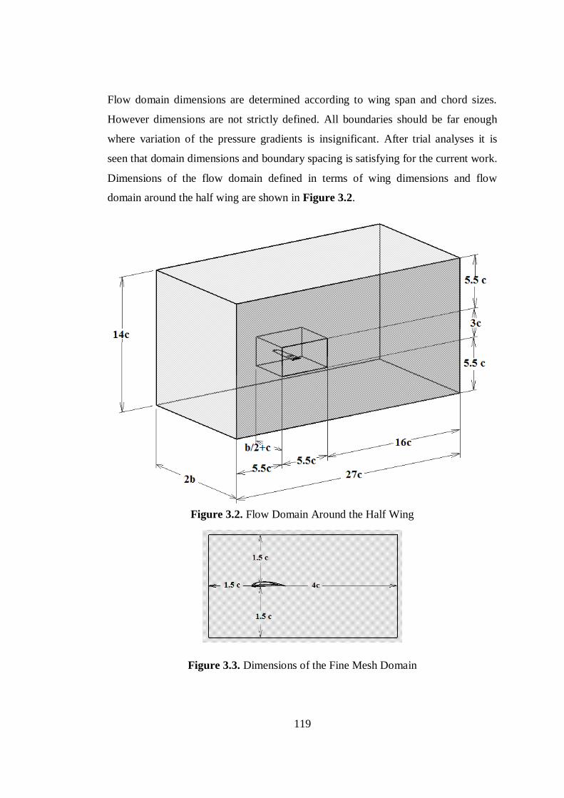
119
Flow domain dimensions are determined according to wing span and chord sizes.
However dimensions are not strictly defined. All boundaries should be far enough
where variation of the pressure gradients is insignificant. After trial analyses it is
seen that domain dimensions and boundary spacing is satisfying for the current work.
Dimensions of the flow domain defined in terms of wing dimensions and flow
domain around the half wing are shown in Figure 3.2.
Figure 3.2. Flow Domain Around the Half Wing
Figure 3.3. Dimensions of the Fine Mesh Domain

120
Investigation of enclosure volume size effects on results are studied by Gölcük [36].
Result of this investigation shows that modification or increasing of enclosure
volume has insignificant effect on CL values. MH114 airfoil is analyzed in the study
and domain size effect results are shown in Figure 3.4. Therefore flow domain is
decided and continued with the current domain sizes.
Figure 3.4. CL Variations According to Flow Domain Adjustment for Different
Mesh Numbers [36]
3.2.1.1. Mesh Generation
Boundary layer mesh (inflation) generation around the wing is one of the most
important steps of the meshing process. Before meshing the enclosure volume, first
layer thickness is needed to be determined. Boundary layer wall distance is
calculated by using relations given in reference [30] for parameters given in Table
3.2.
Table 3.2. Wall Distance Estimation Parameters for Wing Analysis
Dynamic Viscosity 𝜇 1.789 × 10⁻⁵ 𝑘𝑔/𝑚𝑠
Density 𝜌 1.225 𝑘𝑔/𝑚3
Freestream Velocity 𝑈∞ 16.2 𝑚/𝑠
Reference Length 𝑐̅ 0.282 𝑚
Dimensionless Wall Distance 𝑦+ 1

121
Reynolds Number is calculated from,
𝑅𝑒 =𝜌𝑈∞𝑐̅
𝜇 (3.1)
Skin friction coefficient is calculated by using Schlichting correlation,
𝐶𝑓 = [2 log10(𝑅𝑒) − 0.65]−2.3 𝑓𝑜𝑟 𝑅𝑒 < 109 (3.2)
Wall shear stress is calculated as,
𝜏𝑤 = 𝐶𝑓 ⋅1
2𝜌𝑈∞
2 (3.3)
Friction velocity is calculated from,
𝑢∗ = √𝜏𝑤 𝜌⁄ (3.4)
Wall distance is calculated as ,
𝑦 = 𝑦+𝜇 𝜌𝑢∗⁄ (3.5)
And finally, by using equations above, estimated wall distance is calculated as,
𝒚 = 𝟏. 𝟗 × 𝟏𝟎−𝟓 𝒎
By taking calculated first layer thickness into account, inflation and global mesh
sizing settings are set. Mesh around the wing is refined by using the inner enclosure
volume shown as a small rectangular volume in Figure 3.2.Generated mesh domain
and boundary layer mesh around the half wing is shown in Figure 3.5. Mesh
statistics are given in Table 3.3.

122
Figure 3.5. Global Mesh and Boundary Layer Mesh
Table 3.3. Mesh Statistics
Nodes 1225387
Elements 3946868
Minimum Skewness 7.9452e-005
Maximum Skewness 0.96134
Average Skewness 0.22288
Skewness is the measure of mesh quality. Mesh quality with respect to skewness
parameter is given in Table 3.4. According to these parameters, average mesh
quality of the generated mesh is excellent.
Table 3.4. Mesh Quality wrt. Skewness Value [31]

123
Since mesh quality is satisfying, boundary conditions are applied to the domain. As
mentioned before, inlet velocity vector is changed instead of changing the geometric
angle of attack in order to use generated mesh in varying positive angle of attack
analyses. Therefore, “velocity inlet” boundary condition is set to the lower surface of
the enclosure volume and “pressure outlet” boundary condition is set to the upper
surface of the enclosure volume as can be seen in Figure 3.6. Wing surface
boundaries are set to “wall” boundary condition and symmetry plane of the wing and
far side of the enclosure volume are set to “symmetry” boundary conditions which
are shown in Figure 3.7.
Figure 3.6. Boundary Conditions for Velocity Vector with Positive aoa
Figure 3.7. Boundary Conditions of the Global Mesh

124
Mesh convergence study is performed for whether solution converges or not by
decreasing mesh sizes and increasing number of elements. However, determining the
aerodynamic load acting on the wing at limit load is the main objective of CFD
study. Therefore finding a proper pressure data which gives the target loading value
and importing the pressure distribution to the structural mesh is sufficient for the
study. During the structural analysis phase, resultant force calculated from the
imported data is checked and it is seen that target load is achieved. Thus, mesh
convergence study is not covered in the study.
3.2.1.2. Solver and Turbulence Model
Pressure based steady solver is set for solver options and Spalart-Allmaras one-
equation model is chosen as turbulence model. Spalart-Allmaras turbulence model is
developed for aerospace industry and it is low memory and accurate model for low
Reynolds number attached wall-bounded flows [33]. It is reliable for wing analysis
and mesh independency is verified with experimental studies [37].
3.2.1.3. Wing Analysis Results at Limit Load Condition
Wing analysis is performed for various angle of attack values between 3 and 4
degrees. Required loading is determined at 3.8 degree angle of attack. Total lift, drag
and moment values of the half wing, corresponding aerodynamic coefficients and
limit load factor are given in Table 3.5.
Table 3.5. Limit Load Analysis Results for 𝛼 = 3.8°
L 45.2533 N CL 0.917 n 2.31
D 2.69477 N CD 0.05458
M,c/4 -2.39923 N.m Cm,c/4 -0.17232

125
Pressure distribution on the wing is also determined, shown in Figure 3.8. Result is
exported as Nastran input format and applied to the wing structure.
Figure 3.8. Pressure Distribution on the Wing
Upper Surface Lower Surface

126
3.3. Wing Structure Design
Wing structure is designed for two different spar configurations. First configuration
is the classical I Spar configuration, where spar carries shear, axial and bending loads
and distribute and transfer shear loads on the upper and lower surfaces. Closed
section behind the front spar is acting like torque box for this configuration. Second
configuration is the tubular spar configuration which is already a closed section
torque carrying structure. However, in small aircrafts like R/C models, it works as a
bending load carrier due to small cross section. It is preferred to ease manufacturing
which are simply aligned on the tubular spar from rib holes. Aim of choosing to
compare these two spar configuration is to decide which one is safer. Design models
for two different configurations are given in Figure 3.9.
Figure 3.9. Structural Design Models for Different Spar Types
Lightening openings on the ribs shown in Figure 3.9 are not taken into account in
the structural analysis models. By this way stress concentration difference on ribs
due to configuration difference can be examined better since opening sizes are
different. Analysis of the ribs with openings can be studied in a future work.
E-Glass/Balsa composite material is chosen for the thin shell surfaces of the
structures. Stiffeners with rectangular box cross-section and tube spar components
are chosen as extruded carbon/epoxy profiles, which are unidirectional composite
materials with orthotropic material properties. Structural models of the wing
configurations are shown in Figure 3.10 and Figure 3.11. Upper and lower surfaces
are hidden in order to show inner structure.

127
Figure 3.10. Stiffened I Spar Configuration
Figure 3.11. Carbon Tube Spar Configuration
3.4. Material Definitions
Weights of the wings with different spar configurations are kept same by selecting
proper dimensions for carbon structures. E-Glass/Balsa composite component
thicknesses are specified for commercially available 1-2 mm balsa wood. Upper and
lower skin material is 1 mm E-Glass/Balsa and rib-spar materials are 2 mm E-
Glass/Balsa. Material definitions of the wing structure components are given in
Table 3.6.
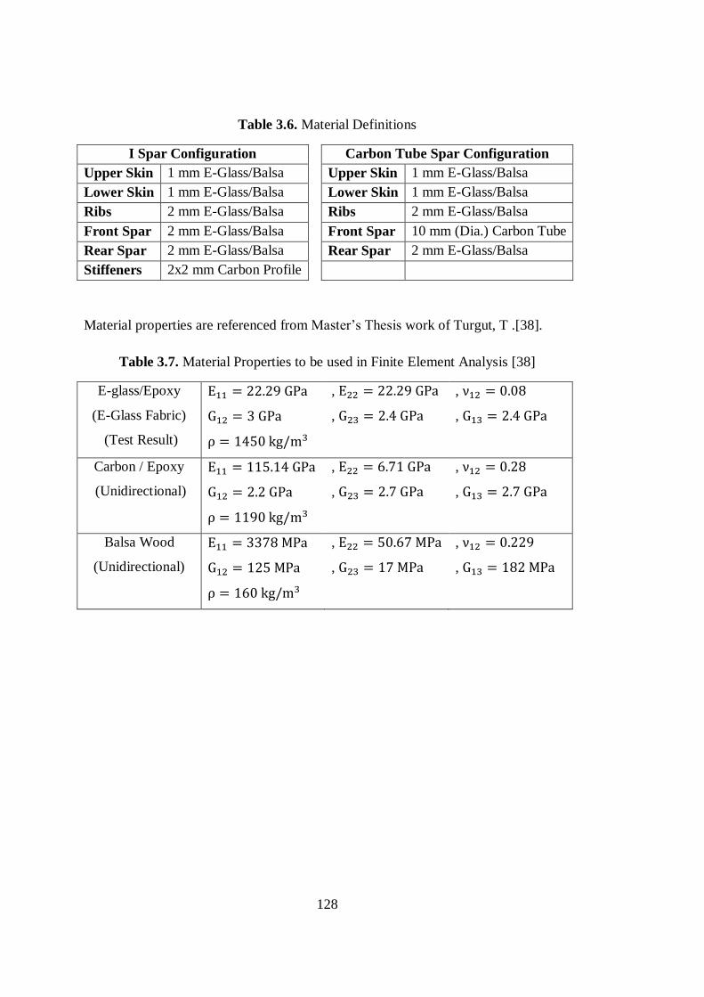
128
Table 3.6. Material Definitions
I Spar Configuration Carbon Tube Spar Configuration
Upper Skin 1 mm E-Glass/Balsa Upper Skin 1 mm E-Glass/Balsa
Lower Skin 1 mm E-Glass/Balsa Lower Skin 1 mm E-Glass/Balsa
Ribs 2 mm E-Glass/Balsa Ribs 2 mm E-Glass/Balsa
Front Spar 2 mm E-Glass/Balsa Front Spar 10 mm (Dia.) Carbon Tube
Rear Spar 2 mm E-Glass/Balsa Rear Spar 2 mm E-Glass/Balsa
Stiffeners 2x2 mm Carbon Profile
Material properties are referenced from Master’s Thesis work of Turgut, T .[38].
Table 3.7. Material Properties to be used in Finite Element Analysis [38]
E-glass/Epoxy
(E-Glass Fabric)
(Test Result)
E11 = 22.29 GPa
G12 = 3 GPa
ρ = 1450 kg/m3
, E22 = 22.29 GPa
, G23 = 2.4 GPa
, ν12 = 0.08
, G13 = 2.4 GPa
Carbon / Epoxy
(Unidirectional)
E11 = 115.14 GPa
G12 = 2.2 GPa
ρ = 1190 kg/m3
, E22 = 6.71 GPa
, G23 = 2.7 GPa
, ν12 = 0.28
, G13 = 2.7 GPa
Balsa Wood
(Unidirectional)
E11 = 3378 MPa
G12 = 125 MPa
ρ = 160 kg/m3
, E22 = 50.67 MPa
, G23 = 17 MPa
, ν12 = 0.229
, G13 = 182 MPa

129
3.5. Structural Analysis of Wing
Structural analyses of the wing configurations are performed to decide which
configuration will be used in the final configuration. Therefore actual stress and
deflection of the wing are not critical for the study and mesh dependency and
convergence of the result studies are skipped. Nevertheless, maximum stress
locations and magnitudes are interested to compare two different configurations.
Finite element models of the wing structures are created on MSC Patran. Structural
components and finite elements representation of the wing configurations are shown
in Figure 3.12.Wing skin, ribs and spar elements are 2D shell elements, stiffener
(Figure 3.13.a) and tubular front spar (Figure 3.13.b) elements are 1D Beam
elements with corresponding cross-sections shown in Figure 3.13.
Figure 3.12. Finite element models of I Spar (a) and Tube Spar (b) Structures
(a)
(b)

130
Elements types and number of elements used in the finite element models are given
in Table 3.8. Note that, two 1D stiffeners are used in the I-spar configuration and
one 1D front spar is used in the tube spar configuration. Additional 2D elements in
CQUAD are come from the front spar elements of I-spar configuration.
Table 3.8. Element Types and Number of Elements of Structural Models
I Spar
Configuration
Tube Spar
Configuration
Structural Element
Element
Type
Number of
Elements
Number of
Elements
Stiffener & Tube Spar (1D) CBAR 220 110
Skin & I-Spar (2D) CQUAD4 7700 7260
Ribs (2D) CTRIA3 2256 2691
Total 10176 10061
The CBAR element is a six degree of freedom general purpose beam that supports
tension and compression, torsion, bending in two perpendicular planes, and shear in
two perpendicular planes. Its formulation is derived from classical beam theory. The
neutral axis may be offset from the grid points which are useful for modeling
stiffened plates [39]. Stiffener element section is shown in Figure 3.13.a and tube
spar section is shown in Figure 3.13.b.
Figure 3.13. CBAR Element Sections (Dimensions are in mm)

131
3.5.1. Boundary Conditions
Defining boundary conditions properly is very important in finite element analysis.
Patran uses to <T1, T2, T3>, <R1, R2, R3> notation to define boundary conditions
and degree of freedoms. Where “T” represents translation, “R” represents rotation
axes in “123” (x, y, z) directions respectively.
Since half wing model is used in the analysis, boundaries of the root rib are
constrained as a symmetry plane (T2=0) As the first boundary condition, root rib is
not allowed to bend in X (chordwise) axis (R1=0) but it is allowed to rotate in Y
(spanwise) axis (R2=1) or move in XZ (symmetry) plane (T1=T3=1) because of the
wing twist. Therefore, first boundary condition is defined as;
BC1: <T1 T2 T3> , <R1 R2 R3> = <101>, <010> = 246
Wing is mounted to the aircraft by clamping the first spar section. Therefore, second
boundary condition is applied to the first spar sections between root rib and second
rib. First sections of the spars are constrained in six degree of freedom which means
they are not allowed to move freely or rotate in any direction.
BC2: <T1 T2 T3> , <R1 R2 R3> = <000> , <000> = 123456
Boundary conditions applied on the root rib and first spar sections are shown in
Figure 3.14 and Figure 3.15.
Figure 3.14. Boundary Conditions of I Spar Structure
BC1: 246
BC2: 123456

132
Figure 3.15. Boundary Conditions of Carbon Tube Spar Structure
Ribs of the structural configuration with carbon tube front spar have circular holes on
the spar locations and tubular spars are modeled with 1D beam elements. Therefore
there is no physical contact between spar holes and 1D spar elements in the finite
element model and nodes on these parts do not coincide with each other. RBE2 type
Multi-Point Constraint (MPC) rigid bar elements (RBE2) are defined in order to
establish rib-spar connection and load transfer. Rib surfaces and 1D spar element is
shown in Figure 3.16 and defined MPC element with connection nodes are shown in
Figure 3.17.
Figure 3.16. Rib Surfaces and Front Spar (Dot)
Figure 3.17. Rib Elements (CTRIA3) and MPC (RBE2) Element
BC1: 246
BC2: 123456

133
3.5.2. Aerodynamic Load Interpolation
Pressure load determined from CFD analysis is applied on the finite element model.
Since CFD mesh has finer mesh with small sized elements and structural elements
have coarser mesh with relatively big elements, mesh and pressure data is needed to
be interpolated on coarser mesh structural model. Original pressure data exported
from CFD and interpolated data contours are shown in Figure 3.18.
Figure 3.18. Pressure Load Interpolation

134
3.5.3. Structural analysis Results
Global stress is concentrated on the upside of the front spar for I spar configuration
and mid panel of the upper surface for carbon tube spar configuration. As can be
seen from Figure 3.19, stress magnitude is higher for carbon tube spar configuration
which means safety factor is smaller.
Figure 3.19. Maximum Equivalent Stresses on the Wing Structures
Maximum stress magnitudes and locations are given in Table 3.9.
Table 3.9. Global Maximum Stress and Deflections
I Spar Location Carbon Tube
Spar
Location
Maximum Stress 10.3 MPa Front Spar 11.9 MPa Skin Panel
Maximum Deflection 5.84 mm Wing Tip
TE
8.62 mm Wing Tip
TE
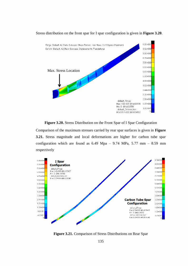
135
Stress distribution on the front spar for I spar configuration is given in Figure 3.20.
Figure 3.20. Stress Distribution on the Front Spar of I Spar Configuration
Comparison of the maximum stresses carried by rear spar surfaces is given in Figure
3.21. Stress magnitude and local deformations are higher for carbon tube spar
configuration which are found as 6.49 Mpa – 9.74 MPa, 5.77 mm – 8.59 mm
respectively
Figure 3.21. Comparison of Stress Distributions on Rear Spar
Max. Stress Location

136
Stress distributions on rib surfaces are shown in Figure 3.22 and Figure 3.23. Again,
local maximum stress magnitude is higher for the carbon tube spar configuration and
stress concentration at the spar hole on the ribs is noticeable while stress is
concentrated at stiffener locations on the front spar for the I spar configuration.
Figure 3.22. Stress Distribution on Ribs of I Spar Configuration
Figure 3.23. Stress Distribution on Ribs of Carbon Tube Spar Configuration

137
In order to compare stress distribution on ribs in detail, third ribs are chosen to
compare which are not constrained by boundary conditions. As can be seen from
Figure 3.24, local stress is concentrated at the stiffener location for I Spar
configuration and stress concentration is maximum at upper mid panel location for
carbon tube spar configuration. Similarly, magnitude of the maximum stress is higher
for the carbon tube spar configuration. Low stress areas on the ribs can also be seen
from stress contours clearly. Blue shaded areas are exposed to smaller stress values
and they can be cut out for lightening. Openings on the rib model shown in Figure
3.9 are perfectly fitted to the low stress locations on ribs. These openings are
considered in the detail design.
Figure 3.24. Comparison of Maximum Stress Distribution on Third Ribs
Figure 3.25. Positions of the Rib Openings

138
3.5.4. Structural Layout of the Wing
Structural layout of the wing is decided after examination of the structural analysis
results. According to these results given in the previous section, I spar configuration
is decided as the final structural layout.
Maximum stresses on the structural components of I spar configuration are lower and
stresses are distributed between rib-spar and wing skin. Furthermore, maximum
bending stress on the structure due to aerodynamic load is concentrated on upper
surface mid panel for the tubular spar configuration while skin stresses are
distributed to the front spar and ribs for I spar configuration.
Concentrated skin stresses of the tubular spar configuration may cause delamination
of the skin material due to buckling problem. If an initial defect of adhesion between
e-glass and balsa layers is assumed, which is highly expected in hand lay-up
manufacturing methods, buckling of the defected area may cause generation and
propagation of the delamination [40].

139
CHAPTER 4
DETAIL DESIGN
4. DETAIL DESIGN
4.1. Introduction
In this chapter, detail design of the aircraft is presented. Overall design and sub-
components of the aircraft are specified and weight of the design is checked to
ensure MTOW of the aircraft constrained by Article (2.3) of SHT-İHA regulations
[13] is not exceeded.
Detail design phase is defined as “nuts and bolts” phase of airplane design.
Designing each individual rib, spar, section and skin takes place of the current design
phase [15] and actual weight of the aircraft is determined by counting weights of
these components. As mentioned, mainly composite materials are used in the current
design, which are manufactured by hand lay-up – vacuum molding methods.
However, uneven material density of balsa core material, possible composite
manufacturing defects due to excess resin usage, over-impregnated or unwetted
zones makes difficult to estimate material weights and reduces precision of the
weight estimation. In order to make more precise weight estimation, composite
material densities are referenced from the previous mini UAV design and
manufacturing project ([41], [42]) studied to experience design and manufacturing
methodology.
Design for manufacturing and assembly (DFMA) and portability issues are also
explained in the detail design phase. Payload bay configurations are presented,
system components are placed and center of gravity location is checked for the detail
design. Finally, design of the aircraft is completed and it is ready to be manufactured
at the end of this study.

140
4.2. Composite UAV Manufacturing Study
In order to experience manufacturing techniques and methodology of a composite
Structure Mini UAV, “HUAVN” hand-launched Mini UAV was designed and
manufactured in a particular study [41], [42]. Composite aircraft components are
manufactured with wet hand lay-up method. General sizing of the HUAVN is given
in Table 4.1 and manufactured UAV is shown in Figure 4.1.
Table 4.1. General Sizing of HUAVN [41], [42]
Empty Weight MTOW Span: b (m) Length: L (m)
2 kg 3 kg 1.8 m 1.15 m
Figure 4.1. HUAVN Composite Mini UAV [41], [42]
Figure 4.2 shows that the manufacturing process of wing and tail skin surfaces while
glass fabric laid on the balsa core material is impregnating with epoxy resin by hand.
Figure 4.2. Wet Lay-up of the Wing-Tail Skin Materials

141
Vacuum bagging is a common application for hand lay-up manufacturing method.
Wetted material laid on the mold is usually consolidated by a vacuum bag and
entrapped air is removed by the vacuum pressure.. Vacuum bagging components are
shown in Figure 4.3.
Figure 4.3. Vacuum Bagging Method [43]
After vacuum bagging and curing processes are ended, final products are ready to be
assembled on the wing and tail structure. Vacuum bagging and final products are
shown in Figure 4.4. After final product weights and dimensions are measured,
average material densities, given in Table 4.2, are determined.
Figure 4.4. Vacuum Bagging of the Wing-Tail Surfaces (a) and Cured Products (b)
Table 4.2. E-Glass/Balsa Material Densities
Skin Material and Thickness Density
E-Glass/Balsa – 1 mm 380 kg/m3
E-Glass/Balsa – 2 mm 280 kg/m3
(a) (b)

142
4.3. Detail Design
Detail design of the aircraft is completed by taking design for manufacturing and
assembly (DFMA) issues and portability into account. Fuselage-wing-tail joints are
also shown in detail in following sections. During the detail design phase, CAD
model of the design is constructed in CATIA. Overall detail design of the aircraft is
shown in Figure 4.5.a. In order to show internal structure of main components
clearly, skin on the aircraft is hidden in Figure 4.5.b.
Figure 4.5. Detail Design of Demircan Mini UAV
( a )
( b )

143
4.3.1. Design for Manufacturing and Assembly
In order to ease manufacturing and decrease product costs, design for manufacturing
and assembly (DFMA) is very important for detail design phase. Design of modular
parts with self-locating and fastening features, design for a base part to locate other
parts [44] features of DFMA is applied on the current design. DFMA also aims to
reduce material, overhead and labor cost. Therefore, internal structures of the
fuselage, wing and tail are all designed with self-locating ribs, spars, bulkheads and
longitudinal frames for the ease of manufacturing. System components of the aircraft
are located on floors which are connected to the respective bulkheads and
longitudinal frames which are the base structures of the fuselage.
Self-locating wing rib placement is shown in Figure 4.6. Firstly ribs are placed from
lower slots on the ribs and fixed with epoxy adhesive to the correspondent slots
located on the spar. Once all ribs are placed and fixed, upper stiffener can be placed
to the upper slots on ribs. Application of the self-locating slot feature is shown in
Figure 4.7.
Figure 4.6. Self-Locating Slot Rib Placement
1. Rib Placement
2. Stiffener Placement
2
2
1
Spar Slots
Rib Slots Upper Stiffener

144
Figure 4.7. Rib Placement Application [42]
4.3.2. Assembly Design
Assembly design is performed to divide aircraft components in portable sizes or
modules in order to satisfy portability requirement. Divided parts of the aircraft can
be re-assembled in the operation field. Motor part is an individual module allows
changing motor, motor mount and motor case together if needed. Components and
assembly design of Demircan Mini UAV is shown in Figure 4.8.
Figure 4.8. Assembly Design of Demircan Mini UAV
Right Wing Section
Left Wing Section
Tail Boom
Motor Module Vert. Tail
Hor. Tail
Fuselage
Payload Bay
Gimbal
Center Wing Section

145
4.3.3. Portability
Portability of the Demircan Mini UAV is the design requirement. Demounted aircraft
should be fitted in a case carried by one personal. Placement of the demounted
aircraft in a case and dimensions of the case is shown in Figure 4.9. Small case
dimensions allow satisfying the portability requirement which are determined
as (1𝑚) × (36 𝑐𝑚) × (40 𝑐𝑚).
Figure 4.9. Demounted UAV in a Case
(Dimensions are in mm)

146
4.3.4. Fuselage – Wing – Tail Joints
Wing – body connection is one of the most problematic issues of DFMA process.
Since bending moment of the wing maximized at the center (symmetry plane) of the
wing, structural failure commonly occurs at the wing center. According to FEM
analysis results, structural stress on the wing root can be distributed by clamping the
spar. Therefore wing center is reinforced with carbon fiber – epoxy layers. In order
to assemble center wing section to the body, carbon tubes are placed to the lower
sides of the front and rear spars as a female joint. Spars and carbon tubes are bonded
together with the carbon fiber – epoxy reinforcement. By this way, clamped like
wing boundary is satisfied as mentioned in the FEM analysis.
Center wing assembly is conducted as follows; firstly wing is aligned to the wing
location then fixed with connector pins from the side holes reinforced by carbon
plate and plywood hard points on the fuselage structure. Finally, connector pins are
secured by fixing the connector caps. Assembly procedure is shown in Figure 4.10.
Detail of the carbon plate and plywood reinforced wing joint on the fuselage is
shown in Figure 4.11.
Figure 4.10. Wing and Body Joints and Assembly
1. Wing Alignment
2. Connector Pin
3. Connector
Cap

147
Figure 4.11. Detail of the Wing Joint on the Fuselage
Joints of the center wing section and outer wing sections are designed as a multi-
joint. Both center wing and outer wing sections and tail boom are assembled at once.
After all components are joined together, wing-boom connector pins are placed to
secure all components at the same time. Meanwhile, flap and aileron servo
connections are also established. Spar extensions on the outer wing enter to the E-
Glass Fiber reinforced plywood guides located on the center wing section. Assembly
procedure of the wing – tail boom is shown in Figure 4.12. Due to limited time,
structural analysis of the wing – tail boom joints are not covered in the current study.
Figure 4.12. Wing and Tail Boom Joints and Assembly

148
Horizontal Tail – Vertical Tail is assembled by fitting screw. Rudder and elevator
servo connections are established at the same time. Tail assembly is shown in Figure
4.13.
Figure 4.13. Horizontal Tail and Vertical Tail Connection
Rudder and servo cables pass through inside of the carbon booms while one boom
carries rudder servo cable; the other boom carries elevator servo cable. Servo
connection diagram is shown in Figure 4.14.
Figure 4.14. Tail Servo Connection Diagram
Horizontal Tail Vertical Tail Vertical Tail
Tail
Boom
Tail
Boom
Rudder - Servo
Connection
Rudder - Servo
Connection

149
4.3.5. Payload Bay
Payload bay is a modular component of the design which may be designed
differently for a particular mission by taking 1.5 kg of maximum payload capacity
into account. For the current design payload bay consists of 3 parts. Main frame and
payload bay hatch are shown in Figure 4.15. ISR Mission payload, the gimbal for
the current design, is located on the front wall of the payload bay which is shown in
Figure 4.16.a.
Figure 4.15. Payload Bay
In order to provide multi-mission capability to the design, different system
components related to the mission can be located to the payload bay. For example, a
gimbal can be attached to the nose for ISR mission (Figure 4.16.a), experimental
data acquisition unit can be placed to the payload bay and a probe can be placed with
a streamlined nose (Figure 4.16.b) and streamlined nose can be attached for different
missions or empty weight flights (Figure 4.16.c).
Figure 4.16. Payload Bay Configurations
(a) (b) (c)

150
4.3.6. Fuselage
Fuselage is mainly constructed from plywood frames. System components are also
mainly attached to the longitudinal frames with individual floor panels. Landing gear
ports are located on the bottom frames and main landing gear port is supported with
two vertical and transverse frames which are directly connected to the carbon plate
reinforcement of wing joints. Hard points of the wing joint are supported by both
fuselage frames and carbon plate reinforcement. Connection point of the motor
module is supported by rear of the longitudinal frames and hard point of the wing
joint. Detail design of the fuselage is shown in Figure 4.17.
Figure 4.17. Detail Design of the Fuselage

151
4.4. System Components
System components of the aircraft are same as given in Section 2.16. During the
conceptual design, system component locations were defined as point masses
roughly. After detail design is completed, all component sizes, locations and weights
are determined more precisely. Aircraft system components located on the fuselage
are shown in Figure 4.18, Component weights and center of gravity locations are
given in the following section.
Figure 4.18. Aircraft System Components Located on the Fuselage
Gimbal
GPS
Camera
Control Unit Telemetry
Battery Pack
Autopilot
Module
Receiver
ESC Motor
Propeller

152
4.5. Weight Check and CG Location
All components of the aircraft are determined and located in the detail design phase.
As mentioned before overall weight and center of gravity location are checked in this
section. Comparison of conceptual design and detail design weight estimations are
given in Table 4.3. Servo weights are included to wing and tail components.
As given in Table 4.3, structural weights used in the conceptual design phase and
detail design results are quite close to each other. Structural weights given in the
conceptual design phase has been estimated by using weight per unit wetted area
values determined from the HUAVN project [41], [42]. Thus, difference between
results is minimized and overall weight estimation of the conceptual design phase is
verified.
Table 4.3. Comparison of Conceptual and Detail Design Weights
Component
Conceptual Design
Weight Estimation
Mass (g)
Detail Design
Weight Estimation
Mass (g)
Wing 860 gr 884.8 gr
Horizontal Tail 170 gr 133.6 gr
Vertical Tail 140 gr 191.2 gr
(Total Tail) ( 310 gr ) ( 324.8 gr)
Fuselage 396 gr 302.7 gr
Prop System 129 gr 122.3 gr
Battery 934 gr 990 gr
Camera System 1140 gr 1130 gr
Avionics 231 gr 257.9 gr
Total Mass 4000 gr 4012.5 gr

153
All components of the detail design and center of gravity locations are given in
Table 4.4. System components are located to ensure center of gravity location is
preserved between 47.2% - 51.6% of the root chord as defined in the conceptual
design chapter. CG location is preserved at 47.95% of the root chord.
Table 4.4. Aircraft System Components and CG Locations of Detail Design
Component Mass (g) CG,x (mm) CG,y (mm) CG,z (mm)
Left Wing 206.6 53.49 658.37 18.217
Center Wing 381.6 66.992 0 9.888
Right Wing 206.6 53.49 -658.37 18.217
Horizontal Tail 118.6 868.013 0 201.456
Vertical Tail 1 80.6 603.138 -333 34.464
Vertical Tail 2 80.6 603.138 333 34.464
Fuselage 302.7 -43.216 0 -53.812
Gimbal 800 -446.546 0 -60
Cam Control Unit 330.0 -179.799 -0.301 -43.002
Motor 109.3 306.175 0 19.868
Propeller 13.0 325 0 19.868
Servo - HT 15.0 870 -15 201.442
Servo - VT 1 15.0 830 -333 82.812
Servo - VT 2 15.0 830 333 82.812
Servo - RF1 15.0 145 440 14.909
Servo - LF1 15.0 145 -440 14.909
Servo - RF2 15.0 155 180 13.14
Servo - LF2 15.0 155 -180 13.14
Servo - RA 15.0 110 860 20.558
Servo - LA 15.0 110 -860 20.558
Main Battery 330.0 105 -34 -88.398
Main / Aux. Battery 330.0 105 0 -88.398
Main Battery 330.0 105 34 -88.398
Receiver 11.0 39.429 0 -30.017
Autopilot Module 40.0 -39.138 0 -30.142
GPS 17.0 -298.803 0 -54.469
Telemetry 50.0 -104.875 13.105 -24.491
ESC 40.0 216.599 0 -12.646
Wiring 100.0 220 0 0
𝚺𝒎 (gr) CG,x (mm) CG,y (mm) CG,z (mm)
4012.5 7.300 0.082 -29.917
XCG (%croot) 47.95%

154
4.6. End of the Detail Design
Detail design phase of the aircraft has been discussed in this chapter. Design for
manufacturing and assembly (DFMA) issues are considered, sub-components of the
aircraft have been specified and weight and center of gravity location of the design
has been checked.
Main purpose of the detail design is to present ready to be manufactured design.
Overall design is constructed in CATIA in detail then weights and center of gravity
location of the design is determined at once. Total weight and center of gravity
location is preserved by making minor design corrections in detail and changing
system component locations slightly. Assembly and portability of the design is also
provided in the detail phase and finally detail design of Demircan Mini UAV is
completed by the end of this phase and it is ready to be manufactured.

155
CHAPTER 5
CONCLUSION
5. CONCLUSION
In this thesis study, aerodynamic and structural design of an electric powered
portable Mini UAV which has variable multi-mission capability is conducted.
Conceptual design, wing analysis and detailed design is the main objective of this
work. Different wing structure configurations are compared by performing finite
element analysis and structural layout for the wing is decided since wing is the main
structural weight contributor. At the end of this study, design is completed and it is
ready for manufacturing.
In the conceptual design phase, detailed performance analysis is completed.
However, drag model of the design is needed to be improved for high camber airfoil
configurations. Therefore it is noticed that CFD analysis for the basic wing and
aircraft configuration should be examined in the early stages of the conceptual design
phase in order to check design parameters.
Dynamic thrust estimation model proposed in the conceptual design chapter is also
needed to be validated experimentally at different altitudes and different motor-
propeller combinations are needed to be studied in terms of propeller pitch, diameter
and electric motor parameters like the KV value of the electric motor in. Detailed
dynamic thrust experiments are suggested to investigate altitude effects (AF) on the
propeller performance and overall propulsive performance for electric powered
aircraft in terms of altitude factor (AF) and power correction factor (PcF).
CFD analysis of the wing is performed for positive low angle of attack (PLA) limit
load condition. However, positive high angle of attack (PHA) limit load condition is
not studied in this work. It is realized that PHA analysis is also important for

156
structural aspects since pressure center shift toward to the trailing edge and it should
have been covered in the study.
Structural analysis of the wing and decision of the structural layout of the wing is
presented but overall analysis of the design is not covered in this study. Especially,
aeroelastic analysis of the twin boom design and impact analyses for landing loads
are suggested for further structural examination.
In conclusion, structure of this thesis is based on design and analysis of an electric
powered portable mini UAV with fixed pitch propeller and design phases are
presented in detail until detailed design. From now on, prototype of the design will
be manufactured and further developments will be completed.
5.1. Future Work
Comprehensive CFD analyses are not covered in this study, only structural load
determination is examined for structural analysis purposes. Therefore, detailed CFD
analysis will be completed for different configuration layouts which are focused on
fundamental parameters of the whole aircraft at different angle of attacks and
altitudes including PHA limit load analysis.
Structural analysis of the joints located on wing and fuselage are not covered in this
study. Structural analysis of the wing is performed only to decide on the structural
configuration of the wing. Including the joints, structural analysis of the aircraft
structure will also be performed as a future work.
Later on, conceptual design process will be optimized by developing a computer
program and aircraft performance calculation results will be validated by detailed
CFD results. Furthermore aircraft performance calculations will be expanded for
fixed pitch propeller propulsion. Detailed propulsion system analysis will be
performed and motor-propeller selection will be optimized for different mission
configurations and altitudes for the design. Finally aircraft will be manufactured
from composite materials as described in the “Detailed Design” chapter and much
more optimized and robust design will be presented.
157
REFERENCES
[1] USICO, European Civil Unmanned Air Vehicle Roadmap: Vol. 1 - Overview,
USICO, 2005.
[2] UAV Types, Retrieved July 2015, from http://www.theuav.com .
[3] NATO, UAS Classification Guide, JCGUAV meeting, September 2009.
[4] Fahlstrom, P. G., Gleason, T. J., Introduction to UAV Systems, 1994
[5] Directory of U.S. Military Rockets and Missiles, Sperry “Flying Bomb”,
Retrieved July 2015, from http://www.designation-systems.net/dusrm/app4/
sperry-fb.html .
[6] Directory of U.S. Military Rockets and Missiles, Kettering Bug, Retrieved July
2015, fromhttp://www.designation-systems.net/dusrm/app4/bug.html .
[7] Directory of U.S. Military Rockets and Missiles, Teledyne Ryan, Reconnaissance
RPV’s,Retrieved July 2015, from http://www.designation-systems.net/ dusrm/m-
34.html.
[8] Directory of U.S. Military Rockets and Missiles, RQ-2 Pioneer, Retrieved July
2015, from http://www.designation-systems.net/dusrm/app2/q-2.html.
[9] JAPCC, Strategic Concept of Employment for UAS in NATO, Jan. 2010
[10] Skylark 1 LE Mini UAV, Retrieved Aug. 2015, from http://dev.defense-
update.com/wp-content/uploads/2011/11/skylark_1-le.jpg
[11] Skrzypietz, T., Unmanned Aircraft Systems for Civilian Missions, BIGS Policy
Paper No. 1, Feb. 2012.
[12] Gur,O. and Rosen,A., Optimizing Electric Propulsion Systems for Unmanned
Aerial Vehicles, Journal of Aircraft, vol. 46, no. 4, pp. 1340 - 1353, July - Aug.
2009.
[13] SHGM (DGCA),SHT-İHA,2015
[14] UAV Vision,CM100,Retrieved July 2015, from http://uavvision.com/wp-
content/uploads/2015/05/UAV_VISION_CM100.pdf.
[15] Anderson, John D., Aircraft Performance and Design, McGraw-Hill, 1999
[16] XFLR5, Retrieved July 2015, from http://www.xflr5.com/xflr5.htm

158
[17] XFOIL, Retrieved July 2015, from http://web.mit.edu/drela/Public/web/xfoil/
[18] Raymer, Daniel P., Aircraft Design: A conceptual Approach, 3rd
Ed., AIAA,
1999.
[19] Gudmundsson, S., General Aviation Aircraft Design, Applied Methods and
Procedures, Butterworth-Heinemann,2014
[20] McCormick, B. W., Aerodynamics, Aeronautics and Flight Mechanics, Wiley,
1979
[21] UIUC Propeller Database – Volume 1, Retrieved July 2015, from http://m-
selig.ae.illinois.edu/props/volume-1/propDB-volume-1.html
[22] Emax, GT2218, Retrieved July 2015, from
http://www.emaxmodel.com/brushless-motor/gt-series-motors/gt2218.html
[23] Ecalc, Retrieved July 2015, from http://www.ecalc.ch/motorcalc.php
[24] PropCalc, Retrieved July 2015, from http://www.drivecalc.de/PropCalc
[25] ATI F/T Sensor: Gamma, Retrieved December 2015, from http://www.ati-
ia.com/products/ft/ft_models.aspx?id=Gamma
[26] National Instruments NI USB – 6211 Device Specifications, Retrieved
December 2015, from http://www.ni.com/pdf/manuals/375195b.pdf
[27] Archer, R. D., Saarlas, M., Introduction to Aerospace Propulsion, Prentice Hall,
1996
[28] Traub, L. W., Range and Endurance Estimates for Battery-Powered Aircraft,
Journal of Aircraft, vol. 48, no. 2, pp. 703-707, March-April 2011
[29] Iris+ Battery, 3dr Store, Retrieved February 2016, from
https://store.3dr.com/products/iris-plus-battery
[30] Y+ Wall Distance Estimation, Retrieved March 2015, from http://www.cfd-
online.com/Wiki/Y_plus_wall_distance_estimation
[31] Bakker. A, Applied Computational Fluid Dynamics: Meshing, Online CFD
Class, Lecture Notes, Retrieved July 2015, from http://www.bakker.org/
dartmouth06/engs150/07-mesh.pdf
[32] ANSYS Fluent, Retrieved February 2016, from http://www.ansys.com/
Products/Fluids/ANSYS-Fluent
[33] ANSYS, Fluent 12.0, User’s Guide, April 2009

159
[34] MSC Nastran, MSC Software, Retrieved February 2016, from
http://www.mscsoftware.com/product/msc-nastran
[35] Patran, MSC software, Retrieved February 2016, from
http://www.mscsoftware.com/product/patran
[36] Gölcük, A. İ., Winglet Design and Analysis for Low Altitude Solar Powered
UAV, MSc Thesis, Middle East Technical University, 2016
[37] Ortiz, A. D., Quiroz, L.E., &Köck, R. A., Aerodynamic Performance Analysis
of a Low-Speed Acrobatic Airplane by Numerical Simulation, Mecánica
Computacional, vol. 21, pp. 378-391, October 2012
[38] Turgut, T. Manufacturing and Structural Analysis of a Lightweight Sandwich
Composite UAV Wing, MSc Thesis, Middle East Technical University, 2007
[39] MSC Software, MSC. Nastran 2001, Getting Started with MSC. Nastran, User’s
Guide, 2004
[40] Bruno, D., Grimaldi, A., Delamination Failure of Layered Composite Plates in
Compression, International Journal of Solids and Structures, vol. 26, issue 3, pp.
313-330, 1990
[41] Demircan, A., Kayran, A, Kurtuluş, D. F., Kompozit Yapılı Mini İHA’lar İçin
Kalıp Üretim Teknikleri ve Aerodinamik Yüzeylerin Üretimi, 4. Ulusal Havacılık
ve Uzay Konferansı, İstanbul, 2012
[42] Demircan, A., Özkanaktı, M. H., Kırdar, V., Sümer, N.N, Portable Mini
UAV: HUAVN, Project Report, Middle East Technical University, 2012
[43] Miravete, A., Processing and Manufacturing, Composite Design Tutorial,
Stanford University, 2009
[44] Boothroyd, G., Dewhurst, P., Knight, W. A., Product Design for Manufacture
and Assembly, CRC Press, 2010

160
APPENDICES

161
APPENDIX A
COMPETITOR MINI UAVS
APPENDIX A: COMPETITOR MINI UAVS
Table A.1. Design Parameters of Competitor UAVs
Competitor 1 2 3 4 5 6 7 8 9 10 11 12 Average
Wing Span 2.74 2.6 2 2.4 2.2 1.5 2.3 1.7 1.83 2.2 1.7 2.5 2.12 m
Length 1.83 1.8 1.2 2.2 1.35
1.32 1.2 1.22 1.2 1.4 1.3 1.46 m
MTOM 4.3 4.5 4.5 5.5 4.5 5 5 3.5
3.8 3.2 2.9 4.23 kg
Vstall
25
32.4
32.4
34
70 11.72 m/s
Vcruise
50 60 65 48.6
50 90
16.14 m/s
Vmax 80 100
111 84.6
90
129 85 80
26.57 m/s
Ceiling 300 3800 4000 5000 3000 2440
2000
3000
2790 m
Range 5 15 15 10 10 10 10 10
5 5 10 9.55 km
Endurance 60 210 80 90 90 90 90 72 60 60 60 60 80 min
Table A.2. References of Competitor UAVs
1 AeroVironment–Pointer http://www.designation-systems.net/dusrm/m-151.html
2 AeroVironmen– Puma AE http://www.designation-systems.net/dusrm/app4/puma.html
3 Baykar –Bayraktar http://baykarmakina.com/sistemler/bayraktar-mini-
iha/?lang=en
4 Elbit –Skylark 1 http://www.israeli-
weapons.com/weapons/aircraft/uav/skylark/Skylark.html
5 Hydra Tech – E1 Gavillan https://www.uvsr.org/docs/Hydra-Technologies_E1.pdf
6 METU – Güventürk
Turgut, T., Manufacturing and Structural Analysis of a
Lightweight Sandwich Composite UAV Wing, MSc.
Thesis, METU, 2007
7 MKU – Terp 2 http://www.airforce-technology.com/contractors/uav/mku-
uav/
8 Nostromo – Cabure 2 http://www.nostromo-defensa.com/eng/cabure.php
9 ST Aero – Skyblade 3 https://www.staero.aero/www/keyoffering.aspx?serkeyid=O
DAwMDAwMTg
10 Tasuma – Hawkeye 2 http://www.tasuma-uk.com/tasuma.php?p=32
11 Tasuma – Hawkeye 3 http://www.tasuma-uk.com/tasuma.php?p=63
12 Top I Vision – Casper 250 http://bernkastelvintners.com/files/Casper250UAV.pdf

162

163
APPENDIX B
COMPONENT DRAG BUILDUP
APPENDIX B: COMPONENT DRAG BUILDUP
V =13.9 m/s 𝜌,1000𝑚 =1.1117 kg/m3
M =0.04 𝜇,1000𝑚 =1.758 × 10⁻⁵ kg/ms
Table B.1. Drag Coefficient Contributions of the Components
Laminar Turbulent 30% - Laminar
70% - Turbulent
Wing
Re 247875
Cf
0.002667 0.005883
FF 0.973500
Q 1
(CD0)Wing 0.005191 0.011448 0.009571
Fuselage
Re 773510
Cf 0.004692
f 7.333333
FF 1.170475
Q 1
(CD0)Fslg - 0.002852 -
Boom
Re 10548
Cf 0.012536
f 82.0
FF 1.205109
Q 1.1
(CD0)Boom - 0.001001 -

164
Table B.2. Drag Coefficient Contributions of Tail Components
Horizontal Tail
Re 136243
Cf 0.003598 0.006682
FF 1.005113
Q 1.08
(CD0)HT 0.001310 0.002432 0.002096
Vertical Tail
Re 145033
Cf 0.003482 0.006592
FF 1.005113
Q 1.08
(CD0)VT 0.000849 0.001605 0.001378

165
APPENDIX C
AERODYNAMIC RELATIONS ASSOCIATED WITH LIFT DRAG AND
FLIGHT VELOCITY
APPENDIX C: AERODYNAMIC RELATIONS ASSOCIATED WITH LIFT
DRAG AND FLIGHT VELOCITY
𝐿
𝐷=𝐶𝐿𝐶𝐷=
𝐶𝐿
𝐶𝐷0 + 𝐾(𝐶𝐿 − 𝐶𝐿,𝐷𝑚𝑖𝑛)2
(C.1)
𝑑(𝐶𝐿/𝐶𝐷)
𝑑𝐶𝐿=𝐶𝐷 − 𝐶𝐿 (2𝐾(𝐶𝐿 − 𝐶𝐿,𝐷𝑚𝑖𝑛))
(𝐶𝐷)2
𝑑(𝐶𝐿/𝐶𝐷)
𝑑𝐶𝐿=
𝐶𝐷0 −𝐾(𝐶𝐿2 − 𝐶𝐿,𝐷𝑚𝑖𝑛
2 )
(𝐶𝐷0 + 𝐾(𝐶𝐿 − 𝐶𝐿,𝐷𝑚𝑖𝑛)2)2 (C.2)
At (𝐶𝐿 𝐶𝐷⁄ )𝑚𝑎𝑥, numerator is zero
𝐶𝐷0 = 𝐾(𝐶𝐿2 − 𝐶𝐿,𝐷𝑚𝑖𝑛
2 ) (C.3)
Lift coefficient at (𝐿 𝐷⁄ )𝑚𝑎𝑥 is determined as,
𝐶𝐿 = √𝐶𝐷0𝐾+ 𝐶𝐿,𝐷𝑚𝑖𝑛
2 (C.4)
By substituting 𝐶𝐿into 𝐿 𝐷⁄ expression, (𝐶𝐿 𝐶𝐷⁄ )𝑚𝑎𝑥 can be determined as,
(𝐿
𝐷)𝑚𝑎𝑥
= (𝐶𝐿𝐶𝐷)𝑚𝑎𝑥
=√𝐶𝐷0
𝐾+ 𝐶𝐿,𝐷𝑚𝑖𝑛
2
𝐶𝐷0 +𝐾 (√𝐶𝐷0
𝐾+ 𝐶𝐿,𝐷𝑚𝑖𝑛
2 − 𝐶𝐿,𝐷𝑚𝑖𝑛)
2
(𝐿
𝐷)𝑚𝑎𝑥
= (𝐶𝐿𝐶𝐷)𝑚𝑎𝑥
= √1
4𝐾𝐶𝐷0+ (𝐶𝐿,𝐷𝑚𝑖𝑛2𝐶𝐷0
)2
+𝐶𝐿,𝐷𝑚𝑖𝑛2𝐶𝐷0
(C.5)

166
𝑉(𝐿/𝐷)𝑚𝑎𝑥is determined bysubstituting 𝐶𝐿 expression into the lift equation.
𝐿 = 𝑊 =1
2𝜌∞𝑉∞
2𝑆𝐶𝐿
𝑉∞ = √2
𝜌∞
1
𝐶𝐿
𝑊
𝑆
𝑉(𝐿/𝐷)𝑚𝑎𝑥 = 𝑉(𝑇𝑅)𝑚𝑖𝑛 = (2
𝜌∞√
𝐾
𝐶𝐷0 +𝐾𝐶𝐿,𝐷𝑚𝑖𝑛2
𝑊
𝑆)
1/2
(C.6)
𝐶𝐿3/2
𝐶𝐷=
𝐶𝐿3/2
𝐶𝐷0 +𝐾(𝐶𝐿 − 𝐶𝐿,𝐷𝑚𝑖𝑛)2 (C.7)
𝑑(𝐶𝐿3/2/𝐶𝐷)
𝑑𝐶𝐿=
3
2𝐶𝐿1/2𝐶𝐷 − 𝐶𝐿
3/2(2𝐾(𝐶𝐿 − 𝐶𝐿,𝐷𝑚𝑖𝑛))
𝐶𝐷2
𝑑(𝐶𝐿3/2/𝐶𝐷)
𝑑𝐶𝐿
=
3
2𝐶𝐿1 2⁄ (𝐶𝐷0 + 𝐾(𝐶𝐿 − 𝐶𝐿,𝐷𝑚𝑖𝑛)
2) − 2𝐾𝐶𝐿
3/2(𝐶𝐿 − 𝐶𝐿,𝐷𝑚𝑖𝑛)
(𝐶𝐷0 +𝐾(𝐶𝐿 − 𝐶𝐿,𝐷𝑚𝑖𝑛)2)2
(C.8)
at(𝐶𝐿3/2
𝐶𝐷⁄ )𝑚𝑎𝑥
numerator of the equation is zero.
3
2𝐶𝐿1 2⁄ (𝐶𝐷0 +𝐾(𝐶𝐿 − 𝐶𝐿,𝐷𝑚𝑖𝑛)
2) − 2𝐾𝐶𝐿
3/2(𝐶𝐿 − 𝐶𝐿,𝐷𝑚𝑖𝑛) = 0
𝐶𝐷0 =1
3𝐾(𝐶𝐿 − 𝐶𝐿,𝐷𝑚𝑖𝑛)(𝐶𝐿 + 3𝐶𝐿,𝐷𝑚𝑖𝑛) (C.9)
and lift coefficient at (𝐶𝐿3/2
𝐶𝐷⁄ )𝑚𝑎𝑥
is determined
𝐶𝐿 = √3𝐶𝐷0𝐾
+ 4𝐶𝐿,𝐷𝑚𝑖𝑛2 − 𝐶𝐿,𝐷𝑚𝑖𝑛 (C.10)

167
By substituting C.10 into C.7,(𝐶𝐿3/2
𝐶𝐷⁄ )𝑚𝑎𝑥
can be determined as,
(𝐶𝐿3/2
𝐶𝐷)
𝑚𝑎𝑥
=
(√3𝐶𝐷0
𝐾+ 4𝐶𝐿,𝐷𝑚𝑖𝑛
2 − 𝐶𝐿,𝐷𝑚𝑖𝑛)
3/2
𝐶𝐷0 +𝐾 (√3𝐶𝐷0
𝐾+ 4𝐶𝐿,𝐷𝑚𝑖𝑛
2 − 2𝐶𝐿,𝐷𝑚𝑖𝑛)
2 (C.11)
C.10is substituted again as 𝑪𝑳∗ in order to simplify further.
(𝐶𝐿3/2
𝐶𝐷)
𝑚𝑎𝑥
=1
4
(𝐶𝐿∗ + 3𝐶𝐿,𝐷𝑚𝑖𝑛)(𝐶𝐿
∗)1/2
𝐶𝐷0 (C.12)
𝑉(𝐶𝐿3/2
𝐶𝐷⁄ )𝑚𝑎𝑥
is determined by substituting 𝑪𝑳∗into the lift equation.
𝑉(𝐶𝐿3/2
𝐶𝐷⁄ )𝑚𝑎𝑥
= √2
𝜌∞
1
𝐶𝐿∗
𝑊
𝑆
𝑉(𝐶𝐿3/2/𝐶𝐷)
𝑚𝑎𝑥
= (2
𝜌∞
𝑊
𝑆(√3𝐶𝐷0𝐾
+ 4𝐶𝐿,𝐷𝑚𝑖𝑛2 − 𝐶𝐿,𝐷𝑚𝑖𝑛)
−1
)
1/2
(C.13)

168
@ (𝐿 𝐷⁄ )𝑚𝑎𝑥
= (𝐶𝐿𝐶𝐷⁄ )
𝑚𝑎𝑥
Table C.1. (CL/CD)max Relations
Symmetrical Cambered
𝐶𝐷0 𝐾𝐶𝐿2 𝐾(𝐶𝐿
2 − 𝐶𝐿,𝐷𝑚𝑖𝑛2 )
𝐶𝐿 √𝐶𝐷0𝐾
√𝐶𝐷0𝐾+ 𝐶𝐿,𝐷𝑚𝑖𝑛
2
(𝐿 𝐷⁄ )𝑚𝑎𝑥
= (𝐶𝐿𝐶𝐷⁄ )
𝑚𝑎𝑥
√
1
4𝐶𝐷0𝐾 √
1
4𝐾𝐶𝐷0+ (𝐶𝐿,𝐷𝑚𝑖𝑛2𝐶𝐷0
)2
+𝐶𝐿,𝐷𝑚𝑖𝑛2𝐶𝐷0
𝑉(𝐿 𝐷⁄ ),𝑚𝑎𝑥
= 𝑉(𝑇𝑅)𝑚𝑖𝑛 (2
𝜌∞√𝐾
𝐶𝐷0
𝑊
𝑆)
1/2
(2
𝜌∞√
𝐾
𝐶𝐷0 +𝐾𝐶𝐿,𝐷𝑚𝑖𝑛2
𝑊
𝑆)
1/2
@ (𝐶𝐿3/2
𝐶𝐷⁄ )
𝑚𝑎𝑥
Table C.2. (CL3/2
/CD)max Relations
Symmetrical Cambered
𝐶𝐷0 1
3𝐾𝐶𝐿
2 1
3𝐾(𝐶𝐿 − 𝐶𝐿,𝐷𝑚𝑖𝑛)(𝐶𝐿 + 3𝐶𝐿,𝐷𝑚𝑖𝑛)
𝐶𝐿 √3𝐶𝐷0𝐾
𝑪𝑳∗ = √
3𝐶𝐷0𝐾
+ 4𝐶𝐿,𝐷𝑚𝑖𝑛2 − 𝐶𝐿,𝐷𝑚𝑖𝑛
(𝐶𝐿3/2
𝐶𝐷⁄ )
𝑚𝑎𝑥
1
4(
3
𝐾𝐶𝐷01 3⁄)
3/4
1
4
(𝑪𝑳∗ + 3𝐶𝐿,𝐷𝑚𝑖𝑛)(𝑪𝑳
∗)1/2
𝐶𝐷0
𝑉(𝐶𝐿3/2
𝐶𝐷⁄ ),𝑚𝑎𝑥 (
2
𝜌∞√𝐾
3𝐶𝐷0
𝑊
𝑆)
1/2
(2
𝜌∞
1
𝑪𝑳∗
𝑊
𝑆)
1/2

169
APPENDIX D
CONSTRAINT EQUATIONS
APPENDIX D: CONSTRAINT EQUATIONS
D.1. Climb Speed Constraint
𝑉𝜃𝑚𝑎𝑥 = 𝑉𝑠𝑡𝑎𝑙𝑙
𝑉𝜃,𝑚𝑎𝑥4 +
𝜂𝑝𝑟(𝑃 𝑊⁄ )(𝑊 𝑆⁄ )
𝜌∞𝐶𝐷0𝑉𝜃,𝑚𝑎𝑥 −
4(𝑊 𝑆⁄ )2𝐾
𝜌∞2 𝐶𝐷0= 0 (D.1)
𝑃𝐴𝑊=4𝐾(𝑊/𝑆)
𝜌∞𝑉𝜃𝑚𝑎𝑥−(𝑉𝜃𝑚𝑎𝑥)
3𝜌∞𝐶𝐷,0
(𝑊/𝑆)
𝑃𝐴𝑊=4𝐾(𝑊/𝑆)
𝜌∞𝑉𝑠𝑡𝑎𝑙𝑙−(𝑉𝑠𝑡𝑎𝑙𝑙)
3𝜌∞𝐶𝐷,0(𝑊/𝑆)
(D.2)
D.2. Maximum Rate of Climb Constraint
(𝑅/𝐶)𝑚𝑎𝑥 =𝜂𝑝𝑟𝑃
𝑊− 𝑉(𝑅/𝐶)𝑚𝑎𝑥
1.155
(𝐿/𝐷)𝑚𝑎𝑥 (D.3)
𝜂𝑝𝑟𝑃
𝑊=𝑃𝐴𝑊
𝑉(𝑅/𝐶)𝑚𝑎𝑥 ≈ 𝑉(𝐶𝐿3/2/𝐶𝐷)
𝑚𝑎𝑥
= (2
𝜌∞
𝑊
𝑆(√3𝐶𝐷0𝐾
+ 4𝐶𝐿,𝐷𝑚𝑖𝑛2 − 𝐶𝐿,𝐷𝑚𝑖𝑛)
−1
)
1/2
(𝐿
𝐷)𝑚𝑎𝑥
= √1
4𝐾𝐶𝐷0+ (𝐶𝐿,𝐷𝑚𝑖𝑛2𝐶𝐷0
)2
+𝐶𝐿,𝐷𝑚𝑖𝑛2𝐶𝐷0

170
𝑃𝐴𝑊= (
𝑅
𝐶)𝑚𝑎𝑥
+(2
𝜌∞
𝑊
𝑆(√3𝐶𝐷0𝐾
+ 4𝐶𝐿,𝐷𝑚𝑖𝑛2 − 𝐶𝐿,𝐷𝑚𝑖𝑛)
−1
)
1/2
×1.155
√ 1
4𝐾𝐶𝐷0+ (
𝐶𝐿,𝐷𝑚𝑖𝑛
2𝐶𝐷0)2
+𝐶𝐿,𝐷𝑚𝑖𝑛
2𝐶𝐷0
(D.4)
D.3. Maximum Speed Constraint
𝐿 = 𝑊 =1
2𝜌∞𝑉𝑚𝑎𝑥
2 𝑆𝐶𝐿 (D.5)
𝑉𝑚𝑎𝑥 = √2(𝑊 𝑆⁄ )
𝜌∞𝐶𝐿, 𝐶𝐿 =
(𝑊/𝑆)1
2𝜌∞𝑉𝑚𝑎𝑥2
(D.6)
(D.7)
𝑃𝐴 = 𝑃𝑅 = 𝑇𝐴𝑉𝑚𝑎𝑥 =𝑊
𝐿/𝐷𝑉𝑚𝑎𝑥 =
𝑊
𝐶𝐿/𝐶𝐷𝑉𝑚𝑎𝑥
𝑃𝐴𝑊=𝑉𝑚𝑎𝑥𝐶𝐿/𝐶𝐷
(D.8)
𝑃𝐴𝑊=
1
𝐶𝐿/𝐶𝐷√2(𝑊 𝑆⁄ )
𝜌∞𝐶𝐿= √
2(𝑊 𝑆⁄ )𝐶𝐷2
𝜌∞𝐶𝐿3 = (
𝐶𝐷
𝐶𝐿3/2)√
2(𝑊 𝑆⁄ )
𝜌∞ (D.9)
𝑃𝐴𝑊=
(
𝐶𝐷0 + 𝐾(
(𝑊/𝑆)1
2𝜌∞𝑉𝑚𝑎𝑥
2− 𝐶𝐿,𝐷𝑚𝑖𝑛)
2
((𝑊/𝑆)
1
2𝜌∞𝑉𝑚𝑎𝑥
2)
3/2
)
√2(𝑊 𝑆⁄ )
𝜌∞
𝑃𝐴𝑊= √
2
𝜌∞(𝐶𝐷0 + 𝐾(
(𝑊
𝑆)
1
2𝜌∞𝑉𝑚𝑎𝑥2
− 𝐶𝐿,𝐷𝑚𝑖𝑛)
2
)((1
2𝜌∞𝑉𝑚𝑎𝑥
2 )3/2
(𝑊/𝑆)) (D.10)

171
D.4. Sustained Level Turn Constraint
𝑛 = {
1
2𝜌∞𝑉∞
2
𝐾(𝑊 𝑆⁄ )[(𝑇𝐴𝑊)−
1
2𝜌∞𝑉∞
2𝐶𝐷0𝑊/𝑆
]}
1/2
(D.11)
𝑛 = {
1
2𝜌∞𝑉∞
2
𝐾(𝑊 𝑆⁄ )[1
𝑉∞(𝑃𝐴𝑊) −
1
2𝜌∞𝑉∞
2𝐶𝐷0𝑊/𝑆
]}
1/2
(𝑃𝐴𝑊) =
1
2𝜌∞𝑉∞
3𝐶𝐷0(𝑊 𝑆⁄ )
+𝑛2𝐾(𝑊 𝑆⁄ )1
2𝜌∞𝑉∞
(D.12)

172

173
APPENDIX E
APC – SLOW FLYER – 11X4.7 PROPELLER DATA
APPENDIX E: APC – SLOW FLYER – 11X4.7 PROPELLER
Table E.1. Propeller Data
J CT CP 𝜼𝒑𝒓
0.087 0.1151 0.0482 0.209
0.107 0.112 0.0477 0.250
0.133 0.1071 0.0468 0.305
0.155 0.1033 0.0461 0.346
0.175 0.0996 0.0454 0.385
0.197 0.096 0.0448 0.422
0.218 0.0921 0.044 0.456
0.241 0.0885 0.0434 0.492
0.264 0.0844 0.0426 0.522
0.287 0.0803 0.0417 0.553
0.31 0.0762 0.0408 0.579
0.33 0.0723 0.0399 0.598
0.347 0.0687 0.039 0.612
0.373 0.0637 0.0376 0.632
0.391 0.0597 0.0364 0.641
0.416 0.0545 0.035 0.647
0.436 0.0494 0.0336 0.644
0.457 0.0442 0.0322 0.628
0.479 0.0386 0.0307 0.603
0.5 0.0333 0.0293 0.568
0.528 0.0254 0.0273 0.491
0.546 0.0203 0.026 0.426
0.571 0.0131 0.0241 0.310
0.59 0.0077 0.0227 0.200
0.615 -0.0001 0.0205 -0.002
0.637 -0.0068 0.0186 -0.234

