aerodynamic analysis of body-strake configurations
TRANSCRIPT

REPORT DOCUMENTATION PAGE Form Approved OMB No. 0704-0188
Public reporting burden for this collection of information is estimated to average 1 hour per response, including the time for reviewing instructions, searching existing data sources, gathering and maintaining the data needed, and completing and reviewing the collection of information. Send comments regarding this burden estimate or any other aspect of this collection of information, including suggestions for reducing the burden, to Department of Defense, Washington Headquarters Services, Directorate for Information Operations and Reports (0704-0188), 1215 Jefferson Davis Highway, Suite 1204, Arlington, VA 22202-4302. Respondents should be aware that notwithstanding any other provision of law, no person shall be subject to any penalty for failing to comply with a collection of information if it does not display a currently valid OMB control number. PLEASE DO NOT RETURN YOUR FORM TO THE ABOVE ADDRESS. 1. REPORT DATE (DD-MM-YYYY)
26-08-2006 2. REPORT TYPE
Final Report 3. DATES COVERED (From – To)
20 February 2005 - 19-Oct-06
5a. CONTRACT NUMBER FA8655-05-1-3005
5b. GRANT NUMBER
4. TITLE AND SUBTITLE
Aerodynamic Analysis of Body-Strake Configurations
5c. PROGRAM ELEMENT NUMBER
5d. PROJECT NUMBER
5d. TASK NUMBER
6. AUTHOR(S)
Dr. Asher Sigal
5e. WORK UNIT NUMBER
7. PERFORMING ORGANIZATION NAME(S) AND ADDRESS(ES) Technion - Israel Institute of Science and Technology Technion City Haifa 32 000 Israel
8. PERFORMING ORGANIZATION REPORT NUMBER
N/A
10. SPONSOR/MONITOR’S ACRONYM(S)
9. SPONSORING/MONITORING AGENCY NAME(S) AND ADDRESS(ES)
EOARD PSC 821 BOX 14 FPO AE 09421-0014
11. SPONSOR/MONITOR’S REPORT NUMBER(S)
Grant 05-3005
12. DISTRIBUTION/AVAILABILITY STATEMENT Approved for public release; distribution is unlimited. 13. SUPPLEMENTARY NOTES
14. ABSTRACT
This report results from a contract tasking Technion - Israel Institute of Science and Technology as follows: The Grantee will investigate methods to improve the rapid aerodynamic prediction of configurations that feature strakes instead of conventional wings. The longitudinal characteristics of body-strake configurations will be estimated using a hybrid approach that will consider two contributions. (1) The linear (potential) contribution will be estimated; (2) The nonlinear contribution of the whole configuration will be estimated based on cross-flow methods. Analytical results will be generated for five baseline configurations and compared with experimental data.
15. SUBJECT TERMS EOARD, Modeling & Simulation, Vortex flows, Aerodynamics
16. SECURITY CLASSIFICATION OF: 19a. NAME OF RESPONSIBLE PERSON SURYA SURAMPUDI a. REPORT
UNCLAS b. ABSTRACT
UNCLAS c. THIS PAGE
UNCLAS
17. LIMITATION OF ABSTRACT
UL
18, NUMBER OF PAGES
52 19b. TELEPHONE NUMBER (Include area code)
+44 (0)20 7514 4299
Standard Form 298 (Rev. 8/98) Prescribed by ANSI Std. Z39-18

Asher Sigal, Ph. D.
15 Zalman Shazar St.
Haifa 34861, Israel
Aerodynamic Analysis of Body-Strake Configurations
Research Report for Grant № FA8655-05-1-3005
Submitted to
US Air Force Research Laboratory
European Office for Aeronautical Research and Development
June 2006

Acknowledgments
This study was partially supported by US Air Force Research Laboratory, European Office for Aeronautical Research and Development, Grant № FA8655-05-1-3005. Project monitors at EOAR&D were Dr. Wayne Donaldson and Dr. Surya Surampudi. I am indebted to my monitors for their interest, for the support and for the trust at times when I could not keep the promised time table. The technical research advisor was Dr. William B. Blake of AFR/VACA, WPAFB. I am appreciative to his long time interest in my technical activity, his advice and support. A. S.
2

Abstract
A cross flow drag coefficient model for finite length body-strake combinations has been developed. The basis for the new model is transonic test results of two-dimensional body-strake combination by Macha. Adjustment for finite body was done based on the empirical correlation for circular bodies by Jorgensen. Additional adjustment considers the relatively large cross flow drag coefficient of strake alone at subsonic Mach numbers. The model was incorporated in component buildup prediction method. The stability derivatives were estimated using the Missile Datcom code. The inviscid contributions to the normal-force and pitching-moment coefficients are based on these stability derivatives. The contribution of the separated cross flow considers body sections with strakes as one unit and uses the new drag coefficient. The method was applied to seven configurations at Mach numbers between 0.9 and 6.8. In most cases good agreements was obtained between predictions by the Missile Datcom code, the new method and test data. The present method gives better results than the Missile Datcom code for two configurations that feature rectangular, or mostly rectangular, strakes. It was observes that when the cross flow Mach number is higher than 1.0, the present method overestimates the normal-force and the stability margin. This implies that the present cross flow drag coefficient model needs further adjustment.
3

Content
Acknowledgments ............................................................................................................. 2
Abstract.............................................................................................................................. 3
Content............................................................................................................................... 4
Nomenclature .................................................................................................................... 5
Introduction....................................................................................................................... 7
Cross-Flow Drag coefficient............................................................................................. 8 Circular Cylinders............................................................................................................ 8
Plain Strakes .................................................................................................................... 8
Circular-Cylinder-Strake combinations........................................................................... 8
Adjustment for Finite Bodies ........................................................................................ 10
Analysis ............................................................................................................................ 15 Contributions Buildup ................................................................................................... 15
Computations................................................................................................................. 15
Validation......................................................................................................................... 16 Benchmark 1.................................................................................................................. 16
Benchmark 2.................................................................................................................. 19
Benchmark 3.................................................................................................................. 21
Benchmark 5.................................................................................................................. 34
Benchmark 6.................................................................................................................. 36
Benchmark 7.................................................................................................................. 38
List of References............................................................................................................ 43
Appendix A...................................................................................................................... 46
Appendix B ...................................................................................................................... 48
Appendix C:..................................................................................................................... 50
4

Nomenclature
a defined by Eqn. (B.6.a)
A defined by Eqn. (B.6.b)
b maximum inclusive span
B width of configuration
c chord of strake
CDc cross-flow drag coefficient of a finite body
Cdo cross-flow drag coefficient of circular cylinder (2-D)
CDo cross-flow drag coefficient of finite circular body
Cd| cross-flow drag coefficient of isolated strake (2-D)
Cd1 cross-flow drag coefficients for s/d→1.0 (2-D)
Cd2 cross-flow drag coefficients for s/d=2.0 (2-D)
Cdφ cross-flow drag coefficient of body-strake cross section (2-D)
CDφ cross-flow drag coefficient of finite length body-strake combination.
CL lift coefficient
Cm pitching-moment coefficient
CN normal-force coefficient
d body diameter
dR reference diameter, maximum body diameter
ℓ length of body
M Mach number
s inclusive span of strake
SP plan-form area
SR reference area, (π/4)dR2
x longitudinal coordinate
xo location of tip of strake
xR reference point for pitching-moment and center of pressure
5

Greek
α angle of attack
Subscripts
1 contribution of inviscid flow
2 contribution of separated cross-flow
New. Newtonian theory
Designation of the components
B body alone
B-S body-strake combination
S strake alone
SU strake unit, strakes with mutual effects with the body
6

Introduction
In recent years there is a growing interest in missile configurations that feature strakes, rather than wings. The advantage of strakes is their small spans, resulting small volume, which is beneficial for internal carriage and launching from canisters. Codes that are based on component buildup methodologies estimate the linear and nonlinear characteristics of the components separately. Thus, the nonlinear contributions of bodies and wings are estimated using different methods or databases. Flow visualization of body-strake combinations, by Verle,1 shows that the leeward vortex wake of body-strake combination is common to the two components, as depicted in Fig. 1. This implies that the contribution of the separated cross flow to the normal-force of the combination may be different than the sum of the contributions of the components. Literature survey yielded only one experimental study of the cross-flow over straked circular cylinders. Macha2, 3 measured the cross-flow drag coefficient of plain cylinders and in combination with strakes at Mach numbers between 0.6 and 1.0 and span to diameter ratios up to 2.0. The objective of the present study is to explore the benefit of using unified body-strake cross-flow drag coefficient in the estimation of the normal-force and center of pressure location of such configurations.
Fig. 1: Flow visualization of the leeward side of a body-strake combination, from Verle.
7

Cross-Flow Drag coefficient
The analysis that follows refers to and depends upon the cross-flow drag coefficient of circular cylinders and two dimensional strips, representing isolated strakes. Thus, these two basic shapes are being reviewed first.
Circular Cylinders Many researchers measured cross flow drag of circular cylinders, Cdo, and several authors, e. g. Hoerner,2 (Chapters XV and XVI) Jorgensen,3 and the British ESDU4 compiled available experimentally obtained drag coefficient data. The latter will be used in the present study because of the extant of data fused into it and the accurate presentation. See Fig 2.
Plain Strakes The main source for cross flow drag coefficient of a strake, CD|, is Lindsey5 who covered Mach numbers up to 0.7. Hoerner2 compiled the available data. (Chapter 15-3) His proposed curve for the subsonic range is presented in Fig. 4 that is discussed in the next section. The value of CD| in the subsonic region is about 2.0.
Circular-Cylinder-Strake combinations As mentioned before, literature survey yielded only one study of the cross-flow drag coefficients of body-strake combinations. Macha6, 7 measured pressure distributions on plain circular cylinders and in combination with strakes. He integrated the pressure distributions to obtain drag coefficients. His tests covered Mach number range of 0.6 to 1.05 and inclusive strake height to diameter (=s/d) ratios of 1.2, 1.55, and 2.0. For Mach numbers 0.6, 0.7, and 0.8 all three stakes were tested. For Mach numbers 0.9 and 1.0, only the narrower two were tested and at Mach number of 1.05, only one. Plain cylinders of various diameters were also tested at Mach numbers between 0.6 and 1.2. The results enabled him to correct for blockage effects. Since only one diameter was tested with strakes, the corrections for these cases were based on the results obtained with plain cylinders.
Schematic from Macha. Fig. 2 also compares Macha’s results for circular cylinders with the correlation of Ref. 4. Good agreement is apparent, except for M=0.9. This finding corroborates the quality of these data. Fig. 3, reproduced from Ref. 6, shows the dependence of cross flow drag coefficients on strake inclusive width-to-diameter ration, for six Mach numbers. It is apparent that Macha included in his charts plain cylinder data at s/r=1.0 and that his curves consider these data. In Section 5.5 of Ref. 6 he refers to the experimentally obtained
8

circumferential pressure distribution and states: “even the smallest strake height-to-diameter ratio, s/d, of 1.2 the strake edge is the dividing point between the positive and suction pressures.” This conclusion is accepted because the edges of the strakes determine the location of the separation points, which cause the pressure jump. It is conjectured that even very narrow strakes will force separation at its edges. Thus, the present curve fitting does not consider no-strake results. Rather, straight lines were fitted to the available data and were extrapolated to s/d=1.0. Since the data are sparse, eye-ball approximation was used. Since there is only one datum for Mach number of 1.05, it was not included. The present fitted straight lines were added to Fig. 3. The available data for Cd| at Mach numbers of 0.6 and 0.7 are also presented for comparison. The values of Cdφ at s/d=1.0 are named Cd1 and those at s/d=2.0, Cd2. The present model for cross flow drag coefficient of body-strake combinations is
Cdφ = Cd1+(Cd2 –Cd1)(s/d-1.0), = (2.0-s/d)Cd1+(s/d-1.0)Cd2 (1)
The line for M=0.9 is anomalous, as is Cdo for that Mach number, and was not taken in further considerations. It is also apparent that Cd2 is close to Cd|. This implies that for s/d≥2.0 the cross flow drag coefficient should be about that of a plain strake. Cd1 and Cd2 are presented in Fig. 4, with Cdo as reference. It is apparent that they follow the trends of Cdo in the transonic region. The ratios K1=Cd1/Cdo and K2=Cd2/Cdo were evaluated for the three subsonic Mach numbers and their averages are K1=1.125 and K2=1.34. The use of these two factors is discussed in the next section. Also shown in Fig. 4 is Cd| from Hoerner2. As indicated before, in the subsonic region, Cd2 ≈Cd|. Jorgensen2, 8 estimates the cross-flow drag coefficient on a winged (or straked) circular body by considering the normal-force acting on the cross sections, as calculated by the Newtonian theory. Cdφ = [CNφ/CNo]New Cdo. (2) With [CNφ/ CNo]Ne = (3/2)(s/d-1/3), based on d, = (3/2)[1.0-(1/3)(d/s)], based on s. (3) This relationship yields Cd1=Cdo and Cd2=1.25Cdo. Recall that the present findings are K1=1.125 and K2=1.34. Namely, the present estimate of Cdφ is larger than Jorgensen’s by a factor of 1.125 to 1.07. Some strakes are actually highly swept, low aspect ratio, Δ wings. Others feature such front ends, followed by rectangular rear parts. In the case of strakes with strong sweep, it is expected that the added normal force, due to separation along the leading and the side edges of the strakes, will be determined by the leading-edge suction analogy devised by
9

Polhamous.9 His prediction, at low speeds, is analogous to CD|=π. Leading-edge suction decreases as Mach number increases and diminishes when the leading-edge becomes sonic. Nevertheless no attempt was done to include this effect in the present analysis. Note: Eqn. (1) is valid for s/d≤2.0. For larger values of s/d, Cdφ=Cd2. However, large values of s/d should be considered wings rather than strakes.
Adjustment for Finite Bodies It is known e. g. Welsh10 and Jorgensen,3 that cross flow drag coefficient of finite bodies is smaller than that of matching two dimensional bodies. Cross flow drag proportionality factor, defined as the ratio between the cross flow drag coefficients of finite to infinite bodies was introduced. Jorgensen3 processed his own experimentally obtained normal-force curves from a previous study (Ref. 11) and obtained an effective finite body cross flow drag coefficient. His results, from Fig. 5 of Ref. 3 are presented in Fig. 5 and compared with Cdo from Ref. 4. It is apparent that in the transonic region there is a noticeable difference between the cross flow drag coefficients of finite and infinite bodies. Based on the available data, an arbitrary model was selected for this work. It consists of “sewing” parts of the available data:
Table 1: Sources of the present cross flow drag coefficient for finite bodies
M range source 0.0 – 0.7 ESDU 0.7 – 0.9 A constant value connecting local
peaks of the two sources 0.9 – 1.2 Jorgensen
1.2 and up ESDU The present model is presented in Fig. 5. It features a dip around M=0.9, and a peak around M=1.1. No smoothing was introduced into the model. Finite body models for CD1 and CD2 were obtained by multiplying finite circular body model by K1 and K2, respectfully. The subsonic branch of the latter was modified to account for the observed proximity of Cd2 to Cd| in that range. The models are depicted in Fig. 6 and a tabular form is shown in Appendix A.
10

Cdo comparison (2-D)
0.0
0.4
0.8
1.2
1.6
2.0
2.4
2.8
3.2
0.0 0.4 0.8 1.2 1.6 2.0
M
Cdo
Cdo, ESDU
Cdo, Macha
Fig. 2: The dependence of Cdo on Mach number, from ESDU and Macha.
11
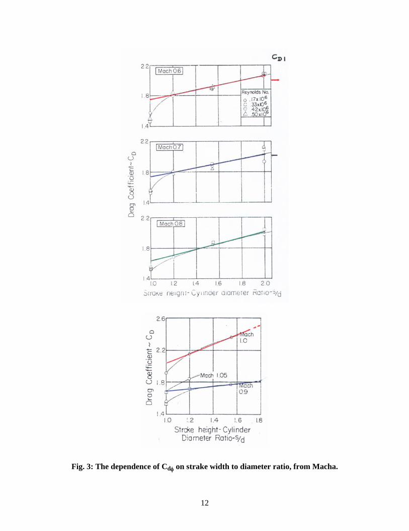
Fig. 3: The dependence of Cdφ on strake width to diameter ratio, from Macha.
12

Cd of straked cylinders (2-D)
0.0
0.4
0.8
1.2
1.6
2.0
2.4
2.8
3.2
0.0 0.4 0.8 1.2 1.6 2.0M
Cd
Cdo, ESDU, Reference.
CD1, Macha, test data
CD2, Macha test data
Plain strake, Hoerner
Fig. 4: Dependence of Cd1 and Cd2 on Mach number.
Cdo / CDo comparison
0.8
1.0
1.2
1.4
1.6
1.8
2.0
2.2
2.4
0.0 0.4 0.8 1.2 1.6 2.0
M
Cdo
, CD
o
Cdo, ESDU
CDo, Jorgensen, finite body
Present CDo
Fig. 5: Comparison between Jorgensen’s CDo and Cdo.
13

CDc (Finite body)
0.8
1.0
1.2
1.4
1.6
1.8
2.0
2.2
2.4
0.0 0.4 0.8 1.2 1.6 2.0M
CD
CDo, ESDU, 2-D
CDo, Finite body
CD1, Finite body
CD2, Finite body
Fig. 6: Present cross flow drag coefficient models.
14

Analysis
Contributions Buildup Following previous researchers, e. g. USAF Datcom12 and Hemsch13, the estimation of the normal-force and pitching-moment coefficients consider two contributions. The first one is that of the inviscid or attached flow, and the second one is due to viscous effects or cross- flow separation.
1. The non viscous contributions are
CN1 = ½ CNα ⋅ sin(2α) (4.a) Cm1 = ½ Cmα ⋅ sin(2α) (4.b)
The two stability derivatives in Eqns. (4) were obtained using the Missile Datcom code (M-Dat, Ref. 14) for zero angle of attack.
2. The present estimation of the contribution of the separated cross flow distinguishes between body sections without and with strakes. For the former, namely for plain circular body, CDo is taken into account, and for the latter, CDφ. These two drag coefficients depend on Mc=M sinα. Thus,
CN2 = ( o
ℓ
∫ CDc B dx)⋅ sin2α /SR (5.a)
Cm2 = ( o
ℓ
∫ CDc B (x-xR) dx)⋅ sin2α /(dRSR) (5.b)
Where ⎧ CDo for plain body sections, CDc = ⎨ (6) ⎩ CDφ for body sections with strakes. ⎧ d for plain body sections, B = ⎨ (7) ⎩ s for body sections with strakes.
Computations Test configurations were divided to longitudinal sections according to their cross sectional shape. For triangular strakes, analytical integration of Eqns. (5.a) and (5.b) were performed to account for the varying span and s/d ratio. For details see appendix B. For rectangular strakes, B=s and Eqn. (1) becomes a constant along the body-strake sections. A service code that calculates Mc for a given Mach number and angles of attach and provides values of the three cross flow drag coefficients was used. The rest of the computations were done on an excel worksheets.
15

Validation
Three types of configurations were selected for the validation of the proposed method:
1. Conical body and Δ wing combinations having common apex. These configurations feature constant s/d, and common center of pressure for both components and both contributions, namely the inviscid and viscous. (Benchmarks 1-2)
2. Bodies and rectangular, or mostly rectangular, strakes. (Benchmarks 3-5) 3. Bodies with Δ strake combinations. (Benchmarks 6-7)
For the first two benchmarks CDφ is constant along the configuration and only depends on Mc. In these cases Eqn. (5.a) reduces to
CN2 = (SP/SR) ⋅ CDc ⋅ sin2α (8)
The center of pressure is at 2/3 the length.
Also, since these configurations are slender, generalized slender body theory, (s-b-t) e. g. Nielsen,14 and Ashley and Landahl,15 was used for a second estimation of the normal-force curve slope.
CNα = 2(s/d)2[1-(d/s)2+(s/d)4] (9)
Benchmark 1 Jorgensen16, in NACA TN 4045, tested a cone-Δ-strake combination at Mach numbers of 1.97 and 2.94. A schematic of his test model is depicted in Fig. 7 and the M-Dat geometrical model is shown in Fig. 8. This model assures the nominal s/d ratio, which is needed for the evaluation of body-strake mutual interference factors. The fineness ratio of the conical body is 3.67, and s/d=1.84. The M-Dat estimates of the normal-force curve slopes are given in Table 1. The estimated center of pressure location is very close to 2/3 body length, as expected.
Table 2 Normal-force curve slope of benchmark 1 configuration
M CNα M-Dat
1.97 4.58 2.94 4.33
16

For s/d=1.84, CDφ = 0.16CD1+0.84CD2. Comparisons between predictions and test data are presented in the two parts of Fig. 9. For M=1.97, the agreements between the two predictions and test data are very good. For M=2.94, the two predictions are very close. However, test data is about linear (CL vs. α) while the predictions show some nonlinearity, causing a slight over-estimate of the lift coefficient.
Fig. 7: Schematic of benchmark configuration 1, from Jorgensen.
Fig. 8: M-Datcom geometrical model of benchmark 1.
17

NACA TN 4045 - B1W1 - M=1.97
0
0.4
0.8
1.2
1.6
2
0 4 8 12 16 20
α
CL
Test data, M=1.97PresentM-Datcom
a)
NACA TN 4045 - B1W1 - M=2.94
0
0.4
0.8
1.2
1.6
2
0 4 8 12 16 20
α
CL
Test data, M=2.94PresentM-Datcom
b)
Fig. 9: Comparison between predictions and test data for benchmark 1, a) M=1.97; and b) M=2.94.
18

Benchmark 2 Foster17, in NASA TM-X-167, tested a cone-Δ-strake combination at Mach numbers of 1.41 and 2.01. A schematic of his test model is depicted in Fig. 10. The conical body has fineness ratio of 4.0, and s/d=2.0, yielding SP/So=10.19. The M-Dat geometrical model is shown in Fig. 11. The estimates of the normal-force curve slopes are given in Table 2.
Table 3 Normal-force curve slope of benchmark 2configuration
M CNα M-dat s-b-t
1.41 6.07 6.5 2.01 5.95 6.5
Since s/d=2.0, CDφ = CD2. Comparisons between analysis and test data are shown in Fig. 12. For M=1.41, M-Dat predicts CN which is up to 10.0% lower than the data. The present estimates are up to 15.0% lower. For M=2.01 the two predictions are in very good agreement with the data.
Fig. 10: Schematic of benchmark 2 configuration, from Foster.
Fig. 11: M-Datcom geometrical model of benchmark 2.
19

NASA TM-X-167 Model 3 M=1.41
-0.5
0
0.5
1
1.5
2
2.5
3
3.5
4
4.5
0 4 8 12 16 20 24 28
α
CN
Test data, M=1.41
M-Datcom
Present
a)
NASA TM-X-167 Model 3 M=2.01
0
1
2
3
4
5
6
7
8
0 4 8 12 16 20 24 28
α
CN
Test data, M=2.01M-DatcomPresent
b)
Fig. 12: Comparison between predictions and test data for benchmark 2, a) M=1.41; and b) M=2.01.
20

Benchmark 3 Reference 11 by Jorgensen contains the database that was used by him to devise the effect of finite body length on the cross flow drag coefficient. In Ref. 19 he tested the same bodies in combination with narrow strakes. Configuration N1-C1-S was selected and is presented in Fig. 13. The geometry of the input model is shown in Fig. 14. The chord of the strake matches the length of the cylindrical afterbody. Span to diameter ratio is 1.2. Reference point for center of pressure location is body base. The stability derivatives of the body alone and of the configuration, as obtained by the M-Dat code are given in table 4.
Table 4 Stability derivatives of benchmark 3 configuration
Body alone Body-strake M CNα Cmα CNα Cmα0.9 2.49 18.07 2.94 20.40 1.2 2.61 19.57 2.97 21.10 1.5 2.48 20.97 6.80 39.22 2.0 2.75 23.27 5.52 24.98
It is apparent that the normal-force curve slope of the configuration is much larger at the two highest Mach numbers than those of the low ones. This is attributed to a jump in the contribution of the fins alone between Mach number 1.2 and 1.5. For the transonic Mach numbers, the normal-force curve slope of the isolated fins is close to those predicted by slender wing theory. In the supersonic range, the values obtained by the code are an order of magnitude larger than those expected by the theory. (The aspect ratio of a pair of strakes is about 0.03.) Comparisons between predictions and test data are presented in the first four parts of Fig. 15, for Mach numbers of 0.9, 1.2, 1.5 and 2.0. At the two low Mach numbers, the present method predicts well the normal-force coefficient, including the local trends, to angles of attack of 50 deg. The estimate of the M-Dat is about 15% lower than the data. At the higher Mach numbers, M-Dat and present predictions of the normal-force coefficient at small and moderate angles of attack are higher than test data. At large angles of attack, the present prediction departs from the test data and remains higher than the data. The departure starts at angles of attack where the cross flow Mach number is about 1.0. At this Mach number the cross flow drag coefficients feature a second hump. Generally, the center of pressure location is well predicted by both methods, except for the dip which is characteristic for the two low Mach numbers. The difference in the initial slopes of the normal-force curves, which was found at M=1.5 and M=2.0, develops noticeable differences at high angles of attack as well. An independent estimate of the slope was sought. Literature search for reliable data for very low aspect ratio rectangular wings did not yield result. Thus, a hybrid estimate was used. The contribution of the body alone was obtained from the M-Dat code. The contribution
21

of the strake unit (strake and mutual interference with the body was estimated using generalized s-b-t. CNα (B-S) = 2⋅(b/d)2⋅[1-(d/b)2+(d/b)4] (10.a) CNα (B) = 2.0 (10.b) CNα (SU) = CNα (B-S) - CNα (B)
CNα (SU) = 2⋅(b/d)2⋅[1-2(d/b)2+(d/b)4] CNα (SU) = 2⋅(b/d)2⋅[1-(d/b)2]2 (11)
For b/d = 1.2, CNα (SU) = 0.269. Thus, for the present case CNα (B-S) = CNα(B) + 0.269. (12) The hybrid estimate of CNα is presented in Table 5. For the lower Mach numbers, the agreement between the two estimates is good. For the higher Mach numbers, the hybrid estimates are smaller than predicted by the M-Dat code. Parts (e) and (f) of Fig. 15 show repeated comparisons between test data and the present method with CNα from both M-Dat, (Present-1) and revised CNα. (Present-2) It is apparent that the estimates that are based on the hybrid approach improves the agreement with test data at small and moderate angles of attack.
Table 5 Comparison of normal-force curve slopes
M B, M-Dat S, M-Dat B-S, M-Dat B-S, Hybr. 0.9 2.49 0.19 2.94 2.76 1.2 2.61 0.09 2.97 2.88 1.5 2.48 1.27 6.80 2.75 2.0 2.75 0.82 5.52 3.02
At larger angles of attack, the revised CN curves still deviate from the test data. As noted before, the deviation occurs around Mc=1.0. This may imply that the cross flow drag coefficient of the present model is a little too high at low supersonic Mach numbers.
22

Fig. 13: Schematic of benchmark 3 configuration, from Jorgensen.
Fig. 14: M-Datcom geometrical model for benchmark 3.
23

NASA TM-X-3130, M=0.9
0
4
8
12
16
20
0 10 20 30 40 50 60
α
CN
Test data, M=0.9M-Datcom, M=0.9Present, M=0.9
NASA TM-X-3130, M=0.9
0
2
4
6
8
10
0 10 20 30 40 50 60
α
X CP/
d
Test data, M=0.9M-Datcom, M=0.9Present, M=0.9
Fig. 15: Comparison between predictions and test data for benchmark 3,
a) M=0.9.
24

NASA TM-X-3130, M=1.2
0
4
8
12
16
20
0 10 20 30 40 50 60
α
CN
Test data, M=1.2M-Datcom, M=1.2Present, M=1.2
NASA TM-X-3130, M=1.2
0
2
4
6
8
10
0 10 20 30 40 50 60
α
X CP/
d
Test data, M=1.2M-Datcom, M=1.2Present, M=1.2
Fig. 15: Comparison between predictions and test data for benchmark 3, b) M=1.2.
25

NASA TM-X-3130, M=1.5
0
4
8
12
16
20
0 10 20 30 40 50 60
α
CN
Test data, M=1.5M-Datcom, M=1.5Present, M=1.5
NASA TM-X-3130, M=1.5
0
2
4
6
8
10
0 10 20 30 40 50 60
α
X CP/
d
Test data, M=1.5M-Datcom, M=1.5Present, M=1.5
Fig. 15: Comparison between predictions and test data for benchmark 3, c) M=1.5.
26

NASA TM-X-3130, M=2.0
0
4
8
12
16
20
0 10 20 30 40 50 60
α
CN
Test data, M=2.0M-Datcom, M=2.0Present, M=2.0
NASA TM-X-3130, M=2.0
0
4
8
12
16
20
0 10 20 30 40 50 60
α
X CP/
d
Test data, M=2.0M-Datcom, M=2.0Present, M=2.0
Fig. 15: Comparison between predictions and test data for benchmark 3, d) M=2.0.
27

NASA TM-X-3130, N1-C1-S, M=1.5
0
4
8
12
16
20
0 10 20 30 40 50 60
α
CN
Test data, M=1.5Present-1, Cn1 from M-DatPresent-2, Cn1 from Hybrid
Fig. 15: Repeated comparison between predictions and test data, benchmark 3,
e) M=1.5.
NASA TM-X-3130, N1-C1-S, M=2.0
0
4
8
12
16
20
0 10 20 30 40 50 60
α
CN
Test data, M=2.0Present-1, Cn1 from M-DatPresent-2, Cn1 from Hybrid
Fig. 15: Repeated comparison between predictions and test data, benchmark 3,
f) M=2.0.
28

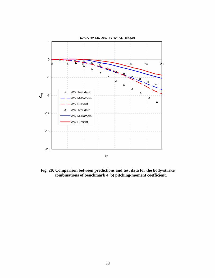
Benchmark 4 From the many configurations that were tested by Robinson,20 in NACA RM L57D19, the three that feature rectangular strakes were selected. Mach number of his tests was 2.01. Schematics of the body and the strakes are depicted in the two parts of Fig. 17. The body consists of a tangent ogive nose with a fineness ratio of 3.5 and a cylindrical afterbody with fineness ratio of 6.5. All strakes have chord to diameter ratio of 4.333. Their span-to-diameter ratios are given in Table 4.
Table 5 Strake span to diameter ratios for benchmark 4 configurations
Configuration b/d F7-W6-A1 4/3=1.333 F7-W5-A1 5/3=1.667 F7-W4-A1 7/3=2.333
A typical M-Dat geometrical model is shown in Fig. 18. Comparison between test data and predictions for the body alone are shown in Fig. 19. At small angles of attack the two methods overestimate the test data. At angles of attack larger than 14.0, the present prediction of the normal-force coefficient is closer to the data than that of the M-Dat. The two estimates of the pitching-moment curve are in very good agreement, however, their nonlinearity are not as pronounced as that of the test data. This accounts for a difference of 0.35 diameters in the center of pressure location. Preliminary comparison between predictions and test data revealed that the predicted normal-force curve slope of configuration F7-W4-A1 is about 28% lower than experimentally observed. As a result, the agreement between prediction and test data is poor at all angles of attack. Thus, this configuration is not included in the discussion that follows. Fig. 20 contains comparisons between estimates and test data for the configurations with the two narrow strakes. The two predictions are very close. The normal-force coefficient for configuration with strakes W5 and W6 are very close to test data. The pitching-moment curves show same trend as body alone, with about the same difference in the center of pressure location.
29

Fig. 16: Schematic of the modular body-strake model, from Robinson.
Fig. 17: M-Datcom input model for configuration F7-W5-A1.
B-S cross flow drag coefficient
0.6
1
1.4
1.8
2.2
2.6
0 0.2 0.4 0.6 0.8 1
Mc
CD
B aloneB-W6, b/d=4/3B-W5, b/d=5/3B-W4, b/d=7/3
Fig. 18: Cross flow drag coefficient for the configurations of benchmark 4.
30

F7-W0-A1 - Body alone
0
1
2
3
4
5
6
0 4 8 12 16 20 24 28
α
CN
Test dataM-DatcomPresent
a)
F7-W0-A1 - Body alone
-4
-3
-2
-1
0
1
2
0 4 8 12 16 20 24 28
α
Cm
Test dataM-DatcomPresent
b)
Fig. 19: Comparison between predictions and test data for the body of benchmark 4, a) normal-force coefficient, and b) pitching-moment coefficient.
31

NACA RM L57D19, F7-W*-A1, M=2.01
0
2
4
6
8
10
12
0 4 8 12 16 20 24 28
α
CN
W5, Test data
W5, M-Datcom
W5, Present
W6, Test data
W6, M-Datcom
W6, Present
Fig. 20: Comparison between predictions and test data for the body-strake combinations of benchmark 4, a) normal-force coefficient.
32
NACA RM L57D19, F7-W*-A1, M=2.01
-20
-16
-12
-8
-4
0
4
0 4 8 12 16 20 24 28
α
Cm
W5, Test data
W5, M-Datcom
W5, Present
W6, Test data
W6, M-Datcom
W6, Present
Fig. 20: Comparison between predictions and test data for the body-strake combinations of benchmark 4, b) pitching-moment coefficient.
33

Benchmark 5 Simpson and Birch21 tested a fineness ratio 19.0 body with three very low aspect ratio wings. Wing 22, which is actually a strake with b/d=1.6 was selected for this work. A schematic of the configuration and the computational model are depicted in Figs. 21 and 22, respectively.
Fig. 21: Schematic of benchmark 5 configuration, from Simpson and Birch.
Fig. 22: Computational model for benchmark 5 configuration.
Comparisons between calculations and test data are presented in Fig. 23. For the body alone, the two predictions are very close and in good agreement with the test data. In the case of the combination, the present estimate of the normal-force coefficient is in very good agreement with the data, while the M-Dat over-predicts it. The predicted center of pressure location is more forward than experimentally observed, with small differences between the two methods. The maximum gap is about 1.5 body diameters at moderate angles of attack and slightly better at higher angles of attack.
34

AIAA-2001-2410
0
2
4
6
8
10
12
0 4 8 12 16 20 24
α
CN
Test data, B-W22M-Datcom, B-W22Present, B-W22Test data, BM-Datcom, BPresent, B
a)
AIAA-2001-2410
-12
-10
-8
-6
-4
-2
00 4 8 12 16 20 24
α
Xcp/
D
Test data, B-W22
M-Datcom, B-W22
Present, B-W22
Test data, B
M-Datcom, B
Present, B
b)
Fig. 23: Comparison between predictions and test data for benchmark 5, a) Normal-force coefficient, and b) center of pressure location.
35

Benchmark 6 Robinson22 investigated at a Mach number of 2.01 a fineness ratio 10.0 body with several wings and controls. Among others, he tested a 5.0 deg delta strake having b/d= 2.07. A schematic of that configuration is shown in Fig. 24. Since b/d>2.0, the strake was divided, lengthwise, into two part. The front one ending at body station where b/d=2.0 was analyzed according to the expression developed in Appendix A. For the rear part CD2 was considered as cross flow drag coefficient. Fig. 26 is a comparison between predictions and test data for this configuration. The two predictions of the normal-force coefficient are close and match the data, except for the present method that slightly overestimates the data past angle of attack of 22.0 deg. There is a slight difference between the two estimates of the pitching-moment curve and the data. The present method predicts stronger nonlinearity in this curve and better predicts the data at high angles of attack.
Fig. 24: Schematic of body with 5o strake, from Robinson.
Fig. 25: M-Datcom geometrical model for Benchmark 6.
36

NACA RM L58A21 5o delta strake
0
1
2
3
4
5
6
7
8
9
10
0 4 8 12 16 20 24 28 32
α
CN
Test dataM-DatcomPresent
a)
NACA RM L58A21 5o delta strake
-14
-12
-10
-8
-6
-4
-2
00 4 8 12 16 20 24 28 32
α
Cm
Test dataM-DatcomPresent
b)
Fig. 26: Comparison between predictions and test data for benchmark 6, a) normal-force coefficient, and b)pitching-moment coefficient.
37

Benchmark 7 Spearman and Robinson23 tested a missile composed of a fineness ratio 10.0 body with low aspect ratio wing and aft control. As can be seen form Fig. 27, the control surfaces are very close to the trailing-edge of the wing, thus were treated as one unit. The geometrical model is depicted in Fig. 28. This benchmark covers Mach numbers of 2.01, 4.65 and 6.8. Comparisons between predictions and test data are presented in the three parts of Fig. 29. For M=2.01, the two predictions are close and in good agreement with test data. The difference in Cm is equivalent to a fraction of body diameter in the center of pressure location. For the two high Mach numbers, the analysis overestimates CN and the absolute value of Cm. In this case too, the present analysis deviates from the trend of the data as Mc=1.0 and higher.
Fig. 27: Schematic of benchmark 7 configuration, from Spearman and Robinson.
Fig. 28: M-Datcom input model for benchmark 7.
38

NASA TM-X-46, M=2.01
0
1
2
3
4
5
6
7
8
9
10
0 4 8 12 16 20 24 28
α
CN
Test dataM-DatcomPresent
NASA TM-X-46, M=2.01
-12
-10
-8
-6
-4
-2
0
2
0 4 8 12 16 20 24 28
α
Cm
Test dataM-DatcomPresent
Fig. 29: Comparison between predictions and test data for benchmark 7,
a) M=2.01.
39

NASA TM-X-46, M=4.65
0
1
2
3
4
5
6
0 4 8 12 16 20 24 28
α
CN
Test dataM-DatcomPresent
-7
-6
-5
-4
-3
-2
-1
00 4 8 12 16 20 24 28
α
Cm
Test dataM-DatcomPresent
Fig. 29: Comparison between predictions and test data for benchmark 7,
b) M=4.65.
40

NASA TM-X-46, M=6.8
0
0.5
1
1.5
2
2.5
3
3.5
4
4.5
5
0 4 8 12 16 20 24 28
α
CN
Test dataM-DatcomPresent
NASA TM-X-46, M=6.8
-6
-5
-4
-3
-2
-1
00 4 8 12 16 20 24 28
α
Cm
Test dataM-DatcomPresent
Fig. 29: Comparison between predictions and test data for benchmark 7, c) M=6.8.
41

Summary and Remarks
1. The longitudinal characteristics of body-strake configurations were evaluated
using component buildup approach that features a unified approach for the estimation of the vortex induced contributions of both components. The new approach uses one cross flow drag coefficient for the part of the body on which the strakes are mounted. The basis for the drag model, are empirical data of Macha who tested straked cylinders in two-dimensional transonic flow. Corrections were made to account for finite body effect and for the cross flow drag coefficient of a plain strake at subsonic Mach numbers.
2. A component buildup method was formulated, that combines non viscous and
viscous contributions to the normal-force and pitching-moment coefficients. For the first contribution, the stability derivatives were obtained using the Missile Datcom code. A unified analysis was used for the other contribution, using the present cross flow drag coefficient model.
3. A pre-processing code was written to obtain the cross flow drag coefficient of
each case as a function of cross flow Mach number and span to diameter ratio. Analytical integration was done for delta strakes where span to diameter ratio varies along the chord.
4. The new method was evaluated by comparing predictions with test data
assembled from the literature. Predictions by the Missile Datcom code were also included for additional comparison. In most cases, the agreements between the Missile Datcom and the present method are good or very good. In the case of two configurations that feature rectangular strakes, the present analysis provides estimates that are much closer to test data than those of the Missile Datcom code.
5. In one case, that features a very low aspect ratio strake, the Missile Datcom code
provided uncertain estimates for the normal-force curve slope of the combination, which is attributed to that of strake alone. A hybrid approach that uses generalized slender body theory and Missile Datcom characteristics for body alone, considerably improved agreement between estimates and test data.
6. The present method gives good estimates as long as the cross flow Mach number
is smaller than 0.95. At higher values, the predictions deviate from the data and the predicted normal-force coefficient is higher than experimentally obtained. This may imply that the present cross flow drag coefficient is a little too high at low supersonic Mach numbers. It is suggested to use additional test data to adjust the present drag model.
7. There is a need for additional test data for body-strake combinations at tri-sonic
Mach numbers.
42

List of References
1. Werle, H., “Tourbillons de Corps Fusseles aux Incidence Eleve,” l’Aeronautique
et l’Astronautique, № 79, June 1979.
2. Hoerner, S. F., “Fluid Dynamics Drag,” Author’s Edition, Midland Park, NJ,
1965.
3. Jorgensen, L. H., “Prediction of Static Aerodynamic Characteristics for Slender
Bodies Alone and With Lifting Surfaces to Very High Angles of Attack,” NASA
TR R-474, Sep. 1977.
4. Anon., “Drag of Circular Cylinders Normal to a Flat Plate With a Turbulent
Boundary Layer for Mach Numbers Up to 3,” ESDU International, Item 83025,
London, UK, 1983.
5. Lindsey, W. F., “Drag of Cylinders of Simple Shapes,” NACA Rep. 619, Oct.
1937.
6. Macha, J. M., “A Wind Tunnel Investigation of Circular and Staked Cylinders in
Transonic Cross Flow,” TAMU Rep. 3318-76-01, Texas A&M Research
Foundation, College Station, TX, Nov. 1976.
7. Macha, J. M., “Drag of Circular Cylinders at Transonic Mach Numbers,” JA, Vol.
14, No. 6, June 1977, pp.605-607.
8. Jorgensen, L. H., “A Method for Estimating Static Aerodynamic Characteristics
for Slender Bodies circular and Noncircular Cross Section Alone and With Lifting
Surfaces at Angles of Attack from 0o to 90o,” NASA TN D-7228, Apr. 1973.
9. Polhamus, E. C., “A Concept of the Vortex Lift of Sharp-Edge Delta Wings
Based on a Leading-Edge-Suction Analogy,” NASA TN D-3767, Dec. 1966.
10. Welsh, C. J., “The Drag of Finite-Length Cylinders Determined from Flight Tests
at High Reynolds Numbers for a Mach Number Range from 0.4 to 1.3,” NACA
TN 2941, 1952.
11. Jorgensen, L. H., and Nelson, E. R., “Experimental Aerodynamic Characteristics
for a Cylindrical Body of Revolution with Various Noses at Angles of Attack
from 0o to 58o and Mach Numbers from 0.6 to 2.0,” NASA TM X-3128, Dec.
1974.
43

12. Hoak, D. E., (Project Engineer) and Ellison, D. E., (Chief Scientist) “USAF
Stability and Control Dactom,” Flight Control Division, AF Flight Dynamics
laboratory, (now AFRL) Wright-Patterson AF Base, OH. 1968.
13. Hemsch, M. J., “Component Build-Up Method for Engineering Analysis of
Missiles at Low-to-High Angles of Attack.” Chapter 4 in “Tactical Missiles
Aerodynamics: Prediction Methods,” Progress in Astronautics and Aeronautics,
Vol. 142, AIAA Publication, 1992.
14. Blake, W. B., “Missile Datcom User’s Manual – 1997 Fortran 90 Version,”
USAF Research Laboratory, Report AFRL-VA-WP-TR-1988-3009, Wright-
Patterson AFB, OH, Feb. 1998.
15. Nielsen, J., “Missile Aerodynamics,” NEAR Inc., Mountain View, CA, 1988.
16. Ashley, H., and Landahl, M., “Aerodynamics of Wings and Bodies,” Addison
Wesley Longman, Reading, MA, 1965.
17. Jorgensen, L. H., “Elliptic Cones Alone and with Wings at Supersonic Speeds,”
NACA TN 4045, 1957.
18. Foster, G. V., “Static Stability Characteristics of a Series of Hypersonic Boost-
Glide Configurations at Mach Numbers 1.41 and 2.01, “NASA TM X-167, Aug.
1957.
19. Jorgensen, L. H., “Experimental Aerodynamic Characteristics for a Cylindrical
Body of Revolution With Side Strakes and Various Noses at Angles of Attack
from 0o to 58o and Mach Numbers from 0.6 to 2.0,” NASA TM X-3130, March
1975.
20. Robinson, R. B., “Aerodynamic Characteristics of Missile Configurations with
Wings of Low Aspect Ratio for various Combinations of Forebodies, Afterbodies,
and Nose Shapes for Combined Angles of Attack and Sideslip at a Mach Number
of 2.01,” NACA RM A57D19, Jun. 1957.
21. Simpson, G. M., “Aerodynamic Characteristics of Missiles having very Low
Aspect Ratio Wings,” AIAA2001-2410, June 2001.
22. Robinson, R. B., “Wind-Tunnel Investigation at a Mach Number of 2.01 of the
Aerodynamic Characteristics in Combined Angle of Attack and Sideslip of
44

Several Hypersonic Missile Configurations With Various Canard Controls,”
NACA RM L58A21, March 1958.
23. Spearman M. L., and Robinson, R. B., “Longitudinal Stability and Control
Characteristics at Mach Numbers of 2.01, 4.65, and 6.8 of Two Hypersonic
Missile Configurations,” NASA TM X-46, Sep. 1959.
45

Appendix A
Tabulated cross flow drag coefficients for finite bodies
Present model for finite length bodies and parameters for the model for body-strake combinations. (See Eqn. 1) CD2 was modified in the subsonic range to account for strake alone cross flow data.
Mc CDo CD1 CD20.00 1.202 1.3523 1.9900 0.04 1.202 1.3523 1.9900 0.08 1.202 1.3523 1.9900 0.12 1.204 1.3545 1.9900 0.16 1.207 1.3579 1.9900 0.20 1.211 1.3624 1.9900 0.24 1.219 1.3714 1.9900 0.28 1.226 1.3793 1.9900 0.32 1.241 1.3961 1.9900 0.36 1.260 1.4175 1.9900 0.40 1.280 1.4400 1.9900 0.44 1.304 1.4670 1.9980 0.48 1.338 1.5053 2.0060 0.52 1.371 1.5424 2.0160 0.56 1.416 1.5930 2.0280 0.60 1.470 1.6538 2.0400 0.64 1.528 1.7190 2.0520 0.68 1.576 1.7730 2.1118 0.70 1.580 1.7775 2.1172 0.72 1.580 1.7775 2.1172 0.74 1.580 1.7775 2.1172 0.76 1.580 1.7775 2.1172 0.78 1.580 1.7775 2.1172 0.80 1.580 1.7775 2.1172 0.82 1.580 1.7775 2.1172 0.84 1.580 1.7775 2.1172 0.86 1.580 1.7775 2.1172 0.88 1.580 1.7775 2.1172 0.90 1.530 1.7213 2.0502 0.92 1.523 1.7134 2.0408 0.93 1.521 1.7111 2.0381 0.94 1.520 1.7100 2.0368 0.95 1.520 1.7100 2.0368 0.96 1.520 1.7100 2.0368 0.98 1.525 1.7156 2.0435
46

Mc CDo CD1 CD21.00 1.530 1.7213 2.0502 1.02 1.545 1.7381 2.0703 1.04 1.565 1.7606 2.0971 1.06 1.590 1.7888 2.1306 1.08 1.635 1.8394 2.1909 1.10 1.645 1.8506 2.2043 1.12 1.650 1.8563 2.2110 1.14 1.650 1.8563 2.2110 1.16 1.640 1.8450 2.1976 1.18 1.630 1.8338 2.1842 1.20 1.610 1.8113 2.1574 1.24 1.576 1.7730 2.1118 1.28 1.542 1.7348 2.0663 1.32 1.516 1.7055 2.0314 1.36 1.492 1.6785 1.9993 1.40 1.470 1.6538 1.9698 1.44 1.450 1.6313 1.9430 1.48 1.436 1.6155 1.9242 1.52 1.419 1.5964 1.9015 1.56 1.408 1.5840 1.8867 1.60 1.400 1.5750 1.8760 1.70 1.376 1.5480 1.8438 1.80 1.359 1.5289 1.8211 1.90 1.343 1.5109 1.7996 2.00 1.327 1.4929 1.7782
47

Appendix B
The Non Linear Normal-Force Coefficient of Body-Δ-Strake Combination
Objective The nonlinear contributions to the normal-force and pitching-moment coefficients as formulated in Chapter Analysis are
CN2 = o
ℓ
∫ CDc B dx · sin2α /SR (B.1.a)
Cm2 = o
ℓ
∫ CDc B (x-xR) dx · sin2α /(dRSR) (B.1.b) Where ⎧ CDo for plain body sections, CDc = ⎨ (B.2) ⎩ CDφ for body sections with strakes. ⎧ d for plain body sections, B = ⎨ (B.3) ⎩ s for body sections with strakes. And
CDφ = (2 – s/d) · CD1 + (s/d – 1) · CD2 (B.3) The integration of Eqns. (B.1.a) and (B.1.b) will be only performed along the chord. For simplicity the range of integration will be from o to c and the reference point will be the apex of the strake. The actual location of the strake will be taken into account during application. Define
IN = o
c
∫ CDc B dx (B.4.a)
Im = o
c
∫ CDc B x dx (B.4.b) The local span is related to the maximum span by s = d + (b-d)⋅x/c (B.5)
48

Define a = (b-d)/c (B.6.a) A = (b-d)/d (B.6.b) Hence s = d + a⋅x (B.7.a) s/d = 1 + a⋅x/d (B.7.b) Introducing Eqn. (B.7.b) into Eqn. (B.3) and CDc B = CDφ s, yields
CDφ = (1- a⋅x/d) ⋅ CD1 + (a · x/d) · CD2 (B.8) Eqns. (B.4) become
IN = o
c
∫ [(1.0-a⋅x/d) · CD1 + (a⋅x/d) · CD2] (d + a⋅x) dx (B.9.a)
Im = o
c
∫ [(1.0-a⋅x/d) · CD1 + (a⋅x/d) · CD2] (d + a⋅x) x dx (B.9.b) Expanding and integrating these expressions and using definition (B.6.b) gives
IN = (c⋅d) ⋅ [(1 - ⅓A2) · CD1 + A · (½ + ½A) · CD2 ] (B.10.a) Im = (c2⋅d) ⋅ [(½ - ¼A2) · CD1 + A · (⅓ + ¼A) · CD2 ] (B.10.b)
Since SR = (π/4) ⋅ d2, this gives CN2 = (4/π) ⋅ (c/d)⋅IN⋅sin2α (B.11.a) Cm2 = (4/π) ⋅ (c/d)2⋅Im⋅sin2α (B.11.b)
49

Appendix C:
Planform Area and Center of Area for Tangent Ogives Geometry: Define:
ℓn
d/2 R
Ð
f = ℓn / d (nose fineness ratio) F1 = f 2 + ¼ F2 = f 2 – ¼
From the schematic, it is apparent that
sin(θo) = ℓn / R cos(θo) = (R–d / 2) / R
using sin2θ + cos2θ = 1, one obtains
R = F1 · d The Ogive Projection Area SS = ½ · θo · R2 (Circular Sector) SΔ = ½ · ℓn · (R–d/2) (Triangle defined by ogive axis and confining radii) Giving Sp = θo · R2 – ℓn · (R–d/2) In the parametric form Sp = d2 · (F1
2 · θo – f · F2) The Ogive Moment of Area relative to the base The aera moment relative to the base of the ogive is
MO = o ℓ ∫ y(x) · x dx
x = R sinθ y = R cosθ – (R–d/2) dx = R cosθ dθ
MO = o θo
∫{R cosθ – (R–d/2)} · R cosθ dθ
50

Integration yields MO = ½ R2 · (R–d/2) · (cos(2θo) – 1) – ⅔ R3 · (cos3θo – 1) Substituting 2cos2 θo-1 for cos2θo, and replacing R with the parametric form,
MO = d3 ·{ F2 · (F22 – F1
2) – ⅔ · (F23 – F1
3)} Normalized form: The projection area is normalized by the circumscribing rectangle. The center of area is normalized by the length of the ogive, and is measured with respect to the base of the ogive. Sp/( ℓn · d) = θo · F1
2 /f – F2 Xc / ℓn = MO/(Sp · ℓn)
= {F2 · (F22 – F1
2) – ⅔ · (F23 – F1
3)} / {f · (F12 · θo – f · F2)}
The normalized forms are presented in Fig. C1.
Tangent Ogive Geometry
0.0
0.1
0.2
0.3
0.4
0.5
0.6
0.7
0.8
0.9
0 1 2 3 4 5f
Sp/(Ln*d)Xc/Ln
Fig. C1: The normalized projection area and center of area of a tangent ogive.
The asymptotic values are 2/3 for the area ratio and 3/8 for the normalized area center.
51