structural and aerodynamic interaction …
TRANSCRIPT

STRUCTURAL AND AERODYNAMIC INTERACTION
COMPUTATIONAL TOOL FOR HIGHLY RECONFIGURABLE WINGS
A Thesis
by
BRIAN JOSEPH EISENBEIS
Submitted to the Office of Graduate Studies ofTexas A&M University
in partial fulfillment of the requirements for the degree of
MASTER OF SCIENCE
August 2010
Major Subject: Aerospace Engineering

STRUCTURAL AND AERODYNAMIC INTERACTION
COMPUTATIONAL TOOL FOR HIGHLY RECONFIGURABLE WINGS
A Thesis
by
BRIAN JOSEPH EISENBEIS
Submitted to the Office of Graduate Studies ofTexas A&M University
in partial fulfillment of the requirements for the degree of
MASTER OF SCIENCE
Approved by:
Chair of Committee, John ValasekCommittee Members, Walter E. Haisler
John E. HurtadoJose RoessetThomas W. Strganac
Head of Department, Dimitris Lagoudas
August 2010
Major Subject: Aerospace Engineering

iii
ABSTRACT
Structural and Aerodynamic Interaction
Computational Tool for Highly Reconfigurable Wings. (August 2010)
Brian Joseph Eisenbeis, B.S., Texas A&M University
Chair of Advisory Committee: Dr. John Valasek
Morphing air vehicles enable more efficient and capable multi-role aircraft by
adapting their shape to reach an ideal configuration in an ever-changing environ-
ment. Morphing capability is envisioned to have a profound impact on the future of
the aerospace industry, and a reconfigurable wing is a significant element of a mor-
phing aircraft. This thesis develops two tools for analyzing wing configurations with
multiple geometric degrees-of-freedom: the structural tool and the aerodynamic and
structural interaction tool. Linear Space Frame Finite Element Analysis with Euler-
Bernoulli beam theory is used to develop the structural analysis morphing tool for
modeling a given wing structure with variable geometric parameters including wing
span, aspect ratio, sweep angle, dihedral angle, chord length, thickness, incidence
angle, and twist angle. The structural tool is validated with linear Euler-Bernoulli
beam models using a commercial finite element software program, and the tool is
shown to match within 1% compared to all test cases. The verification of the struc-
tural tool uses linear and nonlinear Timoshenko beam models, 3D brick element
wing models at various sweep angles, and a complex wing structural model of an
existing aircraft. The beam model verification demonstrated the tool matches the
Timoshenko models within 3%, but the comparisons to complex wing models show
the limitations of modeling a wing structure using beam elements. The aerodynamic
and structural interaction tool is developed to integrate a constant strength source
doublet panel method aerodynamic tool, developed externally to this work, with the

iv
structural tool. The load results provided by the aerodynamic tool are used as inputs
to the structural tool, giving a quasi-static aeroelastically deflected wing shape. An
iterative version of the interaction tool uses the deflected wing shape results from
the structural tool as new inputs for the aerodynamic tool in order to investigate
the geometric convergence of an aeroelastically deflected wing shape. The findings
presented in this thesis show that geometric convergence of the deflected wing shape
is not attained using the chosen iterative method, but other potential methods are
proposed for future work. The tools presented in the thesis are capable of modeling
a wide range of wing configurations, and they may ultimately be utilized by Machine
Learning algorithms to learn the ideal wing configuration for given flight conditions
and develop control laws for a flyable morphing air vehicle.

v
To my parents and sister: Kathy, Kevin, and Laura, for their unwavering support and love

vi
ACKNOWLEDGMENTS
I would like to thank the American Society for Engineering Education for the
National Defense Science and Engineering Graduate Fellowship which provided per-
sonal financial support and enabled me to pursue graduate studies. I would also like
to thank Dr. John Valasek for his mentorship and countless hours of support over the
past few years, as well as Dr. Walter Haisler, Dr. John Hurtado, Dr. Jose Roesset,
Dr. Thomas Strganac, the Vehicle Systems and Control Laboratory at Texas A&M
University, and my family and friends for all of their support throughout my graduate
studies.
This work was sponsored (in part) by the Air Force Office of Scientific Research,
USAF, under grant/contract number FA9550-08-1-0038. The technical monitor was
Dr. William M. McEneaney. The views and conclusions contained herein are those of
the author and should not be interpreted as necessarily representing the official poli-
cies or endorsements, either expressed or implied, of the Air Force Office of Scientific
Research or the U.S. Government.

vii
TABLE OF CONTENTS
CHAPTER Page
I INTRODUCTION . . . . . . . . . . . . . . . . . . . . . . . . . . 1
A. Problem Identification and Significance . . . . . . . . . . . 1
B. Literature Review . . . . . . . . . . . . . . . . . . . . . . . 5
1. Reconfigurable Air Vehicles . . . . . . . . . . . . . . . 5
2. Structure of Reconfigurable Systems . . . . . . . . . . 9
C. Research Issues . . . . . . . . . . . . . . . . . . . . . . . . 11
1. Selection of Structural Analysis Method . . . . . . . . 12
2. Beam Theory Limitations and Accuracy . . . . . . . . 12
3. Modeling of Aeroelastic Effects . . . . . . . . . . . . . 14
D. Research Objectives, Scope, and Methodology . . . . . . . 15
1. Research Objectives and Scope . . . . . . . . . . . . . 15
2. Method . . . . . . . . . . . . . . . . . . . . . . . . . . 17
3. Contributions of This Research . . . . . . . . . . . . . 23
II FINITE ELEMENT ANALYSIS . . . . . . . . . . . . . . . . . . 24
A. Selection of Structural Analysis Method . . . . . . . . . . 24
B. Development of Finite Element Analysis Equations . . . . 25
1. Virtual Work Development of Finite Element Analysis 25
2. Space Frame Stiffness Matrix and Equivalent Nodal
Load Formulation . . . . . . . . . . . . . . . . . . . . 28
3. Space Frame Axis Orientation and Transformation . . 33
4. Assembly of the Global Stiffness Matrix and Solution . 36
5. Post Processing and Axial Stress Analysis . . . . . . . 38
C. Assumptions . . . . . . . . . . . . . . . . . . . . . . . . . . 39
III SPACE FRAME FINITE ELEMENT ANALYSIS
COMPUTATIONAL TOOL DEVELOPMENT . . . . . . . . . . 41
A. Structural Tool Main Program . . . . . . . . . . . . . . . . 41
B. Structural Tool Subroutines . . . . . . . . . . . . . . . . . 43
1. Setup Subroutines . . . . . . . . . . . . . . . . . . . . 43
2. Analysis Subroutines . . . . . . . . . . . . . . . . . . . 44
3. Post Processing Subroutines . . . . . . . . . . . . . . 49

viii
CHAPTER Page
IV SPACE FRAME FINITE ELEMENT ANALYSIS
COMPUTATIONAL TOOL
VALIDATION AND VERIFICATION . . . . . . . . . . . . . . . 54
A. Validation . . . . . . . . . . . . . . . . . . . . . . . . . . . 54
1. Case Description . . . . . . . . . . . . . . . . . . . . . 54
2. Solid Cross Section Case . . . . . . . . . . . . . . . . 56
3. Box Cross Section Case . . . . . . . . . . . . . . . . . 58
B. Verification . . . . . . . . . . . . . . . . . . . . . . . . . . 61
1. Timoshenko Linear Beam Model . . . . . . . . . . . . 61
2. Timoshenko Nonlinear Beam Model . . . . . . . . . . 62
3. 3D Brick Model . . . . . . . . . . . . . . . . . . . . . 65
4. Manureva Wing Model . . . . . . . . . . . . . . . . . 71
V ITERATIVE QUASI-STATIC AEROELASTIC ANALYSIS . . . 79
A. Aerodynamic Tool . . . . . . . . . . . . . . . . . . . . . . 79
B. Integration of Aerodynamic and Structural Tools . . . . . 80
1. Aerodynamic and Structural Interaction Tool . . . . . 80
2. Modification of Aerodynamic Loads . . . . . . . . . . 84
3. Iterative Quasi-Static Aeroelastic Method . . . . . . . 86
C. Analysis of Aeroelastic Results . . . . . . . . . . . . . . . . 89
VI CONCLUSIONS . . . . . . . . . . . . . . . . . . . . . . . . . . . 96
VII RECOMMENDATIONS . . . . . . . . . . . . . . . . . . . . . . 99
REFERENCES . . . . . . . . . . . . . . . . . . . . . . . . . . . . . . . . . . . 101
APPENDIX A . . . . . . . . . . . . . . . . . . . . . . . . . . . . . . . . . . . 106
VITA . . . . . . . . . . . . . . . . . . . . . . . . . . . . . . . . . . . . . . . . 108

ix
LIST OF TABLES
TABLE Page
I Validation Case . . . . . . . . . . . . . . . . . . . . . . . . . . . . . . 55
II Structural Tool Accuracy Compared to Abaqus Results . . . . . . . . 58
III Structural Tool and Abaqus Model Results for Varying Sweep Angles 66
IV Manureva Abaqus Model Structural Components . . . . . . . . . . . 72
V Manureva Wing Structure Geometry Parameters . . . . . . . . . . . 74
VI Structural Tool Manureva Loads . . . . . . . . . . . . . . . . . . . . 75
VII Geometric and Aerodynamic Iteration Results, No Twist Adjustment 90
VIII Geometric and Aerodynamic Iteration Results, Twist Adjustments
Included . . . . . . . . . . . . . . . . . . . . . . . . . . . . . . . . . . 93

x
LIST OF FIGURES
FIGURE Page
1 Wing Geometry and Nomenclature . . . . . . . . . . . . . . . . . . . 3
2 Airfoil Geometry and Nomenclature . . . . . . . . . . . . . . . . . . 4
3 Grumman F-14 (left) and North American Rockwell B-1 (right) . . . 6
4 Wing Morphologies for Hawks (Left) and Pigeons (Right) [8] . . . . . 7
5 Variable Gull-Wing Morphing Aircraft Model [10] . . . . . . . . . . . 7
6 Spider Plot Comparison of Fixed and Morphing Wing Aircraft [15] . 8
7 Batwing Model in the NASA Langley TDT Wind Tunnel [15] . . . . 9
8 Iterative Aerodynamic and Structural Interaction . . . . . . . . . . . 22
9 Rotation of Axes for a Space Frame Member [27] . . . . . . . . . . . 34
10 Structural Tool Main Program . . . . . . . . . . . . . . . . . . . . . 42
11 GEOMETRY Subroutine . . . . . . . . . . . . . . . . . . . . . . . . 44
12 MODIFY INPUTS Subroutine . . . . . . . . . . . . . . . . . . . . . 45
13 ELEMENT VALUES Subroutine . . . . . . . . . . . . . . . . . . . . 46
14 ASSEMBLE K Subroutine . . . . . . . . . . . . . . . . . . . . . . . . 47
15 ASSEMBLE Q Subroutine . . . . . . . . . . . . . . . . . . . . . . . . 48
16 PLOT DEFLECTION Subroutine . . . . . . . . . . . . . . . . . . . 50
17 PLOT DEFLECTION 3D Subroutine . . . . . . . . . . . . . . . . . 51
18 STRESS Subroutine . . . . . . . . . . . . . . . . . . . . . . . . . . . 52
19 PLOT STRESS 3D Subroutine . . . . . . . . . . . . . . . . . . . . . 53

xi
FIGURE Page
20 Linear Euler-Bernoulli Analysis, Deflection due to Lift, Basswood
Solid Cross Section . . . . . . . . . . . . . . . . . . . . . . . . . . . . 56
21 Linear Euler-Bernoulli Analysis, Abaqus Axial Stress due to Lift,
Basswood Solid Cross Section . . . . . . . . . . . . . . . . . . . . . . 57
22 Linear Euler-Bernoulli Analysis, Structural Tool Axial Stress due
to Lift, Basswood Solid Cross Section . . . . . . . . . . . . . . . . . . 57
23 Linear Euler-Bernoulli Analysis, Rotations due to Pitching Mo-
ment, Basswood Solid Cross Section . . . . . . . . . . . . . . . . . . 59
24 Linear Euler-Bernoulli Analysis, Deflections due to Lift, Basswood
Box Cross Section . . . . . . . . . . . . . . . . . . . . . . . . . . . . 60
25 Linear Euler-Bernoulli Analysis, Rotations due to Pitching Mo-
ment, Basswood Box Cross Section . . . . . . . . . . . . . . . . . . . 60
26 Linear Timoshenko Analysis, Deflections due to Lift, Basswood
Solid Cross Section . . . . . . . . . . . . . . . . . . . . . . . . . . . . 62
27 Linear Timoshenko Analysis, Deflections due to Lift, Basswood
Box Cross Section . . . . . . . . . . . . . . . . . . . . . . . . . . . . 63
28 Nonlinear Timoshenko Analysis, Deflections due to Lift, Bass-
wood Solid Cross Section . . . . . . . . . . . . . . . . . . . . . . . . 64
29 Nonlinear Timoshenko Analysis, Rotations due to Pitching Mo-
ment, Basswood Solid Cross Section . . . . . . . . . . . . . . . . . . 64
30 Nonlinear Timoshenko Analysis, Deflections due to Lift, Balsa
Box Cross Section . . . . . . . . . . . . . . . . . . . . . . . . . . . . 65
31 Abaqus 3D Brick Element Model, 30 Degree Sweep Angle, Axial Stress 67
32 3D Brick Element and Structural Tool Comparison for Deflection
with Sweep . . . . . . . . . . . . . . . . . . . . . . . . . . . . . . . . 67
33 3D Brick Element and Structural Tool Comparison for Rotation
with Sweep . . . . . . . . . . . . . . . . . . . . . . . . . . . . . . . . 68

xii
FIGURE Page
34 3D Brick Element and Structural Tool Comparison for Deflection
with Sweep . . . . . . . . . . . . . . . . . . . . . . . . . . . . . . . . 69
35 Structural Tool, 30 Degree Sweep Angle, Axial Stress . . . . . . . . . 70
36 Manureva Aircraft . . . . . . . . . . . . . . . . . . . . . . . . . . . . 71
37 Manureva Wing Abaqus Deflections . . . . . . . . . . . . . . . . . . 73
38 Manureva Wing Deflections, Material Comparison . . . . . . . . . . . 76
39 Manureva Wing Deflections, Boundary Condition Comparison . . . . 77
40 Manureva Wing Abaqus Axial Stress . . . . . . . . . . . . . . . . . . 77
41 Manureva Wing Structural Tool Axial Stress . . . . . . . . . . . . . . 78
42 Non-Iterative Aerodynamic and Structural Interaction Main Program 81
43 Iterative Aerodynamic and Structural Interaction Main Program . . 82
44 Panel Arrangement . . . . . . . . . . . . . . . . . . . . . . . . . . . . 83
45 Panel Lift and Moment Locations . . . . . . . . . . . . . . . . . . . . 85
46 Lift, Drag, and Moment Locations along Principal Axis . . . . . . . . 87
47 Wing Displacements due to Lift . . . . . . . . . . . . . . . . . . . . . 88
48 Deflected and Undeflected Wing Shape . . . . . . . . . . . . . . . . . 89
49 Converged Coefficient of Lift, No Twist Adjustment Case . . . . . . . 91
50 Converged Dihedral Angle, No Twist Adjustment Case . . . . . . . . 91
51 Axial Stress for Converged Manureva Wing . . . . . . . . . . . . . . 92
52 Coefficient of Lift, Twist Adjustment Case . . . . . . . . . . . . . . . 94
53 Twist Angle, Twist Adjustment Case . . . . . . . . . . . . . . . . . . 95
54 Research Schedule Gantt Chart . . . . . . . . . . . . . . . . . . . . . 107

1
CHAPTER I
INTRODUCTION
This chapter states the engineering problem which will be addressed by the research
and identifies the significance and impact that a reconfigurable wing may have on
the aerospace engineering field. This chapter will also discuss some of the history of
the morphing wing problem and will highlight key literature addressing this research
issue. Finally, the chapter will describe the research issues, objectives, scope, and
methods.
A. Problem Identification and Significance
When the Wright Brothers first flew in 1903, their plane had flexible wings which were
warped during flight for better control. As planes began to fly at faster speeds, it
became necessary to use structurally stiff wings to accommodate higher wing loading.
In different flight regimes, there is an optimum wing shape that provides the best
performance for the given flight conditions. Morphing, which is the changing from one
geometrical shape to another, can be used to improve the aerodynamic performance
of an aircraft wing in different flight regimes.
A morphing air vehicle will have an immense impact on the aerospace industry.
In modern society, efficiency is critical and this new technology could allow planes
to be more fuel efficient. Morphing technology will give each plane a wider range of
roles or possible mission objectives and allow the aircraft to be more versatile. The
military currently has certain aircraft that are used for specific tasks such as speed,
range, or maneuverability. One morphing aircraft could possibly fulfill various roles
The journal model is IEEE Transactions on Automatic Control.

2
by changing its geometry. Using only one plane for numerous types of missions would
save money and be more effective.
There are many parameters of a wing that can be effectively morphed to impact
the flight of the aircraft. Parameters defining the cross-sectional airfoil may also be
morphed to improve the wing performance. Parameters defining the wing and airfoil
include the following:
• b Wing span
• S Wing area
• Λ Sweep angle
• Γ Dihedral angle
• αr Root incidence angle
• αt Tip incidence angle
• cr Root chord length
• ct Tip chord length
• tr Root thickness
• tt Tip thickness
Other airfoil properties may also be used for morphing but will not be addressed in
the research. Figure 1 below shows various parameters of a wing. Figure 2 shows
several airfoil parameters which may be effectively morphed.
There are numerous challenges associated with the development of a morphing
air vehicle. The actuation mechanics provide a significant challenge, especially when

3
Fig. 1. Wing Geometry and Nomenclature
multiple degrees of freedom are utilized for morphing. Multiple actuators must be
controlled quickly and simultaneously, and it may be necessary to locate these ac-
tuators throughout the entire wing. Materials also provide a challenge because the
wing must be structurally stiff but capable of changing shape. Many morphing air
vehicles use smart materials to allow for large shape changes. Also, deciding which
morphed geometry is best suited for the current flight condition is another difficulty
of morphing. To make a decision regarding the wing and airfoil parameter values,
a strong understanding of the current aerodynamic and structural implications is
needed. With multiple wing and airfoil morphing parameters, an infinite number of
morphed wing configurations are possible. Because it is necessary to have aerody-

4
Fig. 2. Airfoil Geometry and Nomenclature
namic and structural knowledge for all of these cases, robust and accurate aerody-
namic and structural tools are needed to determine the wing shape which provides
the best aerodynamic and aeroelastic characteristics while maintaining the structural
integrity of the wing. Aeroelasticity is the relationship between the aerodynamic
loads and structural deformations, and the primary parameters of interest include
the lift, aerodynamic pitching moment, displacements, and rotations. All of the pre-
viously mentioned challenges must be addressed in order to effectively fly and control
a morphing air vehicle.
The research will take a general approach and consider a hypothetical morphing
wing which can have large geometric changes in various wing and airfoil parameters.
The goal is to develop the methods needed to analyze the structural and aerodynamic
effects of the general morphing wing and create an analysis and simulation tool. By
developing computational tools for a general morphing wing, the same analysis tools
can be used for multiple aircraft which have different morphing capabilities.
It will be necessary to utilize a structural analysis tool and an aerodynamic
analysis tool. The structural analysis tool will use Finite Element Analysis (FEA)
and work in conjunction with an existing Computation Fluid Dynamics Doublet Panel
Method tool used to model and simulate aerodynamic effects on a morphing wing
[1], [2]. The aerodynamic forces provided by the aerodynamic tool will be used by

5
the structural tool to determine the deflected wing geometry as well as the axial
stresses within the wing. By iterating between the aerodynamic and structural tools,
a converged solution for the deflected wing geometry may be obtained, providing
insight to the quasi-static aeroelastic wing properties.
The ultimate use of the method and tool is to work within a framework which
utilizes various Machine Learning tools that can analyze the aerodynamic and struc-
tural data for a wing at a given flight condition to determine the configuration for
optimal wing geometry [3], [4], [5]. The structural tool will generate the deflections
and stresses based on the input aerodynamic loads and the wing configuration. The
deflection and stress values will be passed to the Machine Learning algorithms for
numerous morphing cases at various flight conditions, so realistic deformations and
stresses are utilized. If stresses exceed the material limitations, the Machine Learning
algorithm will determine a different shape or flight condition in order to maintain the
structural integrity [6], [7].
B. Literature Review
The general focus of the research is on reconfigurable air vehicles, and the specific
area of focus is on the structure of reconfigurable systems.
1. Reconfigurable Air Vehicles
In the past, planes such as the Grumman F-14 and the North American Rockwell B-1
have used mechanical actuation to employ variably swept wings, allowing for better
performance during supersonic flight. These planes are shown in Figure 3.
Since the F-14 and B-1, considerable advancements have been accomplished in
the field of morphing air vehicles. Many of the recent studies of morphing aircraft have

6
Fig. 3. Grumman F-14 (left) and North American Rockwell B-1 (right)
been inspired by nature. A group at Cornell University has analyzed various birds
and their wing shapes at different speeds. Instincts help the birds find the optimal
shape for morphing their wings [8]. Figure 4, taken from Wickensheiser, shows the
various wing shapes for a hawk and a pigeon at different speeds. This reference along
with Reference [9] discuss the aerodynamic performance and dynamic impacts due to
morphing.
Others, such as the University of Florida, have also looked to nature for morph-
ing in flight. Florida University has developed a flapping type model which is shown
in Figure 5 [10]. In Reference [11], Motamed and Yan discuss the use of a flapping
wing for an insect size micro aerial vehicle (MAV). This reference describes the im-
plementation of a reinforcement learning algorithm on a dynamically scaled unsteady
aerodynamic model at low Reynolds numbers. The experimental results show that
the reinforcement learning method is valid for the MAV control problem. Reference
[12] describes the use of an aerodynamic shape optimization program to obtain the
optimal airfoil shape for a given flight condition of a light unmanned air vehicle. The
program is based on a computational fluid dynamics solver with the Spalart-Allmaras

7
Fig. 4. Wing Morphologies for Hawks (Left) and Pigeons (Right) [8]
Fig. 5. Variable Gull-Wing Morphing Aircraft Model [10]
turbulence model and a sequential-quadratic-programming algorithm.
The United States Defense Advanced Research Projects Agency (DARPA) and
Northrop Grumman, completed extensive testing on their morphing program called
Smart Wing. This program developed a hingeless, smart-materials-based, control
surface and wind tunnel tested it in two phases. Phase 1 tested the technology on a
half span F-18 wing and Phase 2 tested it on a full-span unmanned combat air vehicle.
Shape Memory Alloy (SMA) torque tubes and piezoelectric motors were used in dif-

8
ferent tests to actuate the morphing. The wind tunnel studies by Northrop Grumman
have demonstrated improvements in lift, roll moment, and pitching moment making
the aircraft more efficient and more controllable [13]. Testing also showed significant
improvements in the pressure distribution over a smart morphing wing test article by
delaying the flow separation at the trailing edge [14].
Morphing technology will give each plane a wider range of roles or possible mis-
sion objectives as demonstrated by the NextGen Morphing Aircraft Structures (N-
MAS) Program. This study and wind tunnel test completed by DARPA, the Air
Force Research Laboratory (AFRL), and NextGen Aeronautics concluded that mor-
phing aircraft are very beneficial for a mission with hunter-killer parameters. For
this mission type, morphing aircraft could theoretically reduce the sortie rate by 30%
for vehicles less than 20,000 lbs which means fewer aircraft would be needed. This
same study also compared the performance of a morphing vehicle versus a fixed wing
aircraft as shown in Figure 6 below [15]. As shown in Figure 6, the morphing aircraft
Fig. 6. Spider Plot Comparison of Fixed and Morphing Wing Aircraft [15]

9
is far superior to the fixed wing aircraft in every performance category. A picture of
the N-MAS wind tunnel test is shown in Figure 7.
Fig. 7. Batwing Model in the NASA Langley TDT Wind Tunnel [15]
2. Structure of Reconfigurable Systems
Reference [16] discussed the aerodynamic and structural impacts of variable-span
morphing used on a cruise missile. A subsonic doublet-hybrid method panel code
was used to analyze the aerodynamics. It showed that increasing the wingspan im-
proved the aerodynamic properties by increasing the lift while reducing the drag,
leading to an increased range. Anti-symmetric span changes led to improved roll
control. The structural and aeroelastic characteristics of the variable-span wing were
investigated using an MSC/NASTRAN model of the wing-box structure. The model
used two wings sections with the extendable wing section constrained to the main
wing. Analysis showed that when the span increased, the torque at the wing root
decreased considerably and increased at the wing tip slightly, so a variable-span mor-
phing wing does not require a larger wing torsional stiffness. Results also showed
that the bending moment for the extended wing increased dramatically, requiring a

10
need for an increased bending stiffness. Static aeroelastic analysis showed that the
wing tip deformations increased with an increase in span, and the divergence bound-
ary considerably decreased so the extended wing experienced divergence at a lower
dynamic pressure.
Reference [17] describes and validates the structural and aerodynamic tools used
for the static aeroelastic analysis of a morphing wing. Equivalent plate continuum
models for the structure were utilized rather than a discrete finite element approach,
and the aerodynamic loads were provided by an incompressible, quasi-steady vortex
lattice code. Three equivalent plate methods were discussed: Classical Plate The-
ory (CPT), First-order Shear Deformation Theory (FSDT), and Higher-order Shear
Deformation Theory (HSDT). A wing box was modeled using CPT and FSDT, and
the mass and stiffness matrices for the spars, spar caps, ribs, rib caps, and skin were
combined to obtain the wing mass and stiffness matrices. The CPT and FSDT mod-
els were validated using a NASTRAN finite element model, and FSDT proved to
be more accurate. Because the aerodynamic loads depend upon the structural de-
flections, a feedback-loop between the aerodynamics and structure was necessary. A
preliminary case showed aerodynamic coefficient and vertical displacement results at
varying sweep angles.
In Reference [18], Nguyen develops the governing structural dynamic equations
of motion for a flexible wing and accounts for the coupling of the aeroelasticity of
flexible airframe components, the inertial forces due to rigid-body accelerations, and
the propulsive forces. Wing bending and twist degrees of freedom are included in
the structural dynamics equations. A finite-element method was used to solve for
the aeroelastic deflections. The analysis assumes for high aspect ratio wings the
equivalent beam approach with equivalent stiffness properties accurately captures
the elastic behavior and structural deflections of the wing.

11
Many groups have conducted research on the technology needed for the structure
of a morphing vehicle. Reference [19] discusses the use of an actuation system to
accomplish spanwise curvature that allows for near-continuous bending of a wing. The
two actuation systems described and tested were a tendon-based DC motor actuated
system and a SMA-based mechanism. Reference [20] discusses the internal structure
of the same spanwise bending wing. This reference also discusses the need for a
compliant skin which would cover the wing joints and allow for in-plane stretching of
the skin, while maintaining flexural rigidity.
Reference [21] describes various types of smart materials used for morphing ac-
tuation. It specifically describes the adaptive structures used in the Smart Wing
program, and it discusses various adaptive control surfaces and SMA based actua-
tion systems. Reference [22] shows the importance of shape estimation for deforming
structures, and it investigates three types of shape sensing systems. Reference [23]
explored the use of a dynamic shape control system for a morphing airfoil which con-
sisted of two beams pinned at either end. The results showed that the actuation and
control systems successfully and accurately commanded the airfoil shape.
C. Research Issues
This section discusses some of the issues that will be addressed in the research. As
stated in Section I, the primary research objective will be to develop a Finite Element
Analysis tool which can be used for analysis of a morphing wing. To successfully
and accurately achieve the overall research goal, several key research issues must be
addressed.

12
1. Selection of Structural Analysis Method
Various types of elements may be used for Finite Element Analysis including Euler-
Bernoulli beam elements, shell elements, and brick elements. Beam elements are used
to approximate long, slender members; shell elements are used to approximate thin
surfaces; brick elements are used to approximate three dimensional objects. Because
brick and shell elements are more computationally intensive, beam elements are the
most reasonable method provided the wing is relatively long and slender. [24], [25]
Because the thickness of the wing is much smaller than the span, beam elements are
feasible if the chord length is small compared to the span which is the case for a
normal to high aspect ratio wing.
Linear or nonlinear analysis may be used in Finite Element Analysis. The re-
search will pursue a linear method to simplify the computations. Linear analysis is
very accurate when the deformations are relatively small when compared to the size
of the overall structure and when there are not large torsional effects present.
2. Beam Theory Limitations and Accuracy
The linear beam element was selected for its simplicity and computational speed as
opposed to more complex elements such as three dimensional brick elements. By
modeling the aircraft wing as a structural beam so beam theory may be used, several
geometric limitations are placed on the wing. A major research issue will be to
determine the limitations on the wing and to clarify the accuracy of the structural
analysis method. By using beam elements, the cross section will be idealized as having
the area and moments of inertia of a rectangular solid or box and will not be capable
of modeling a curved airfoil shape.
The linear Finite Element Analysis is fairly accurate for a beam which is in

13
bending and has small deflections. If large torsional loads are applied, a highly twisted
wing is used, or the deflections are large, it may be necessary to use nonlinear analysis
to obtain an accurate solution. Linear beam theory also ignores the stiffening effect
produced with large deformations. If the material used for the wing is highly flexible,
a linear analysis will not be sufficient. A flexible material will also exhibit coupling
between the two transverse bending degrees of freedom which must be accounted for
in the off-diagonal terms within the stiffness matrix.
The Finite Element Model will include various wing geometric parameters which
could invalidate the linear beam theory assumption if the parameters become too
large. If the thickness and chord length become very large when compared to the
wingspan or if the twist angle becomes large, linear beam theory will no longer hold.
A highly swept wing under aerodynamic loading will exhibit bending and torsion cou-
pling, but basic beam theory FEA will assume these parameters are uncoupled. The
cantilevered boundary conditions of a highly swept wing may also not be accounted
for using beam theory because there may be significant differences between the stress
concentrations of the forward and aft sections near the root chord of an actual wing.
The bending and torsion coupling and the boundary conditions lead to limitations on
the maximum sweep angle [26]. If morphing is achieved by deforming the structure so
the sweep and dihedral angles undergo large changes compared to their undeformed
angles, linear beam theory will also no longer hold. The research will need to de-
termine the limitations of the aforementioned parameters. The research will need to
quantify the limitations as well as the accuracy associated with changing each pa-
rameter. It will likely be necessary to compare the analysis findings with those of a
commercial FEA program which uses fully three dimensional elements or nonlinear
beam analysis for several different wing configurations. By comparing with a more
accurate FEA program, a numerical quantity can be determined for the accuracy of
14
the finite element code.
3. Modeling of Aeroelastic Effects
1. The research must successfully use the structural analysis in conjunction with
the aerodynamic analysis and determine a deflected wing shape. The loads
which will be input into the FEA code will be generated by a specific doublet
panel aerodynamic code which was developed in MATLAB for the morphing
problem. When the FEA determines a deflected wing shape, the new shape will
have a different set of aerodynamic loads. An iterative method of alternating
between the aerodynamic and structural codes will be necessary to converge on
a final deflected shape for the wing. The process for this iterative approach will
need to be determined and it will be a critical aspect of the research.
2. The aerodynamic code was not developed to accept a curved, deflected wing
shape. The aerodynamic code is set up so that the wing parameters such as
the dihedral and sweep angles are single inputs, and it assumes the wing is
straight. This means that the output shape determined by the FEA code will
not be accurately represented in the aerodynamic code during the iterations. It
will likely be necessary to determine effective changes in the sweep and dihedral
angles which can approximate the deflection. Although the aerodynamic and
aeroelastic properties of a deflected wing are different than those of a straight
wing, the deflections will be small and it may be accurate to represent the
deflected wing with a straight wing. This method will allow for the use of
iterations to converge upon a deflected wing shape.

15
D. Research Objectives, Scope, and Methodology
This section describes the objectives and scope of the research and outlines the plan
and methodology to achieve these goals.
1. Research Objectives and Scope
The objective is to develop a method and computational tool to analyze the structural
and aeroelastic effects exhibited by a wing with geometry changes up to 30%. The
structural tool must determine the deflections and stresses for a given wing configura-
tion and must work with an existing constant strength source doublet panel method
aerodynamic code which provides aerodynamic loads [1], [2]. The aerodynamic and
structural tools must be integrated to converge on a deflected wing shape, providing
insight into the quasi-static aeroelastic properties of the wing. The stresses calculated
by the FEA tool along with the structural limitations for the wing material must ulti-
mately be used by Machine Learning tools [3], [4], [5], [6], [7]. These tools determine
the optimum morphing configurations to give the best aerodynamic characteristics
while also maintaining the structural integrity of the wing.
Although commercial FEA tools exist which are capable of yielding the required
structural analysis results, an in-house FEA code should be developed so it may be
easily integrated with the existing tools and modified to account for future require-
ment changes. Because the existing Machine Learning and aerodynamic tools were
developed using MATLAB, the structural tool should also be developed in MATLAB
so all of the tools are compatible.
An important aspect will be to quantify the accuracy of the structural tool
because it uses various assumptions which are inherent in beam theory, as mentioned
in the Research Issues section. The accuracy must be used to determine the ranges

16
of the morphing parameters where the FEA tool can accurately represent the wing.
The structural tool must provide results accurate within 10% when compared to an
actual aircraft in order for the tool to be reasonably utilized for future morphing wing
modeling purposes.
The scope of the research investigates several significant aspects of the morphing
wing problem. The structural and aerodynamic tools must be capable of analyzing
the following:
1. Variable wing geometry
(a) Sweep angle
(b) Dihedral angle
(c) Incidence angle and twist
(d) Taper ratio
(e) Thickness
(f) Aspect ratio
2. Aerodynamic Tool
(a) Low speed, inviscid, and incompressible flow
(b) NACA 4-Series root and tip airfoils
(c) Output aerodynamic loads
3. Structural Tool
(a) Box or solid wing cross section
(b) Output deflections and rotations
(c) Output axial stress

17
Once the Space Frame Finite Element tool is developed, the questions to be
investigated are:
1. Can the structural and aerodynamic codes be used in conjunction through an
iterative approach to show the quasi-static aeroelastic properties of a deflected
morphing wing? The limitations of the aerodynamic code, as discussed the
Research Issues section, will need to be considered.
2. How can the structural and aerodynamic codes be accurately and efficiently
integrated to produce results which will be of practical use for the Machine
Learning tools?
3. What are the limitations of the FEA code due to the various assumptions from
using linear analysis and beam theory? How can the accuracy with these lim-
itations be quantified? Limitations on the deflections as well as the geometric
morphing parameters must be established.
4. Is the FEA tool correctly yielding the expected linear Euler-Bernoulli beam
theory results?
2. Method
A commercial FEA program, Abaqus, will be used to develop several comparison
cases to validate that the FEA code is generating the correct results. Using linear
Euler-Bernoulli beam analysis in Abaqus, the structural tool, which also uses linear
Euler-Bernoulli beam analysis, will be validated for the following load cases:
1. Pure bending due to lift or drag
2. Pure torsion due to aerodynamic moment

18
There are many limitations associated with a linear FEA code which uses Euler-
Bernoulli beam elements. In order to quantify the accuracy associated with the code,
Abaqus will be used to develop several comparison wing models. Timoshenko beam
theory is capable of accounting for shear deformations and is a more accurate beam
model than Euler-Bernoulli beam theory. The structural tool will be compared to pure
bending and pure torsion cases modeled using Timoshenko beam theory to verify the
accuracy of the structural tool. One of the assumptions inherent in linear analysis is
that the deflections are small when compared to the overall scale of the structure. By
using nonlinear beam analysis in Abaqus, a more accurate representation of the wing
will be observed. The test cases will consist of various flexural stiffnesses to determine
if the given cases are within the linear range. By comparing the results between the
Abaqus model and the Space Frame FEA code, an estimate of the structural tool
accuracy for each case will be determined. As the deflections increase with higher
load magnitudes, the associated accuracy will decrease.
Because a swept wing under aerodynamic loading experiences bending and tor-
sion coupling and the cantilevered boundary conditions become more complex, 3D
brick elements should be used in Abaqus to analyze the accuracy of the structural
tool for a swept wing case. By using various sweep angle cases, the sweep angle lim-
itations for the tool will be determined. Because beam theory is only valid for long,
slender beams, 3D elements may also be used to create various aspect ratio wings
to test the limitations on the aspect ratio. A real world aircraft wing has a more
complex internal structure than a beam. The structure may have various materials
and structural components such as spar caps, spar shear webs, ribs, skin, and a wing
carry-through structure. An Abaqus model of a real wing should be compared to the
structural tool. The verification cases are shown below:

19
1. Timoshenko Beam Model using Abaqus
(a) Pure bending due to lift or drag
(b) Pure torsion due to aerodynamic moment
2. Nonlinear Beam Analysis using Abaqus
(a) Pure bending due to only lift or drag
(b) Pure torsion due to aerodynamic moment
3. 3D Brick Element Analysis with Full Aerodynamic Loading using Abaqus
(a) Various sweep angles
(b) Various aspect ratios
4. Complex Wing Model using Abaqus
(a) Various structural tool stiffnesses
(b) Various structural tool boundary conditions
The code integration issue will be addressed by developing an overarching com-
puter code which will be used to organize the interaction of the aerodynamic and
structural tools. These tools must be setup as function files which may be accessed
by the main program. The main program must first establish the values of the mor-
phing parameters for the current wing configuration as discussed in Section I. The
morphing parameters will then be used as inputs to the aerodynamic and structural
tools.
The aerodynamic tool must be utilized first to output values necessary to calcu-
late the force and moment loads acting on the wing. The doublet panel method uses
a grid which covers the upper and lower surfaces of the wing, and the grid is divided

20
into chordwise and spanwise panels for both the left and right sides of the wing. Be-
cause the aerodynamic tool is setup to calculate the lift and moment coefficients at
each panel and the total drag coefficient, the main program will need to modify the
aerodynamic coefficients to obtain the lift, drag, and pitching moment loads acting
on each element. Beam elements are used in the structural tool, so there is only
one element for each span station. The chordwise lift and moment values must be
combined for each span station, so only one lift force and pitching moment is applied
to each element. The total drag force will be proportionally applied to each element.
The structural tool will use the geometric morphing parameters along with the
lift, drag, pitching moment, and load locations as inputs. The tool will be setup so
the element spacing is tied to the panel spacing of the aerodynamic tool. Because
the structural tool will solve a cantilevered beam problem, it can only handle half of
the wing at a time. The main program must call the structural tool function twice to
obtain the deflection and axial stress values for the entire wing. These values along
with the aerodynamic coefficients may be used by various Machine Learning tools to
determine the next morphed wing shape needed for aerodynamic effectiveness and
wing structural integrity. The aerodynamic and structural tool integration process is
described below:
1. An overarching main program will integrate the aerodynamic and structural
tools
2. Input morphing geometry parameters must be selected
3. The aerodynamic tool function file will be called using the morphing geometry
inputs and it will output aerodynamic coefficients
4. The main program will modify the aerodynamic coefficients to obtain lift, drag,

21
and pitching moment loads at each spanstation
5. The structural tool function file will be called once for each half span of the
wing using the morphing wing geometry, loads, and load locations as inputs
and it will output the wing deflections and axial stresses
6. The aerodynamic coefficients, wing deflections, and stresses may be used by
Machine Learning tools to determine the next morphed wing geometry
An iterative approach which incorporates the structural and aerodynamic tools
may show more realistic quasi-static aeroelastic deflections. Each iteration will cal-
culate the aerodynamic loads and the structural deflections due to those loads. The
iterations will use the new deflected geometry found during the previous iteration to
generate new aerodynamic loads. The rotation deflections cause a change in the twist
angle of the wing, so an updated twist angle will be used as an input to the aero-
dynamic tool. Because the aerodynamic code was not designed to handle a curved,
deflected wing, the bending deflections will need to be converted to an approximate
change in the dihedral and sweep angles. The maximum deflection is located at the
wing tip, so the maximum adjusted dihedral and sweep angles may be determined
using the angle between the wing root and wing tip. These adjusted dihedral and
sweep angles will be used as inputs for the aerodynamic code. Modified wing span
and aspect ratio values should be calculated to account for the new dihedral and
sweep angles, and these values should also be used as inputs for the aerodynamic
tool. This iteration process can be continued until a converged, deflected wing shape
is observed. The steps for the iterative quasi-static linear aeroelastic analysis method
are shown as follows:
22
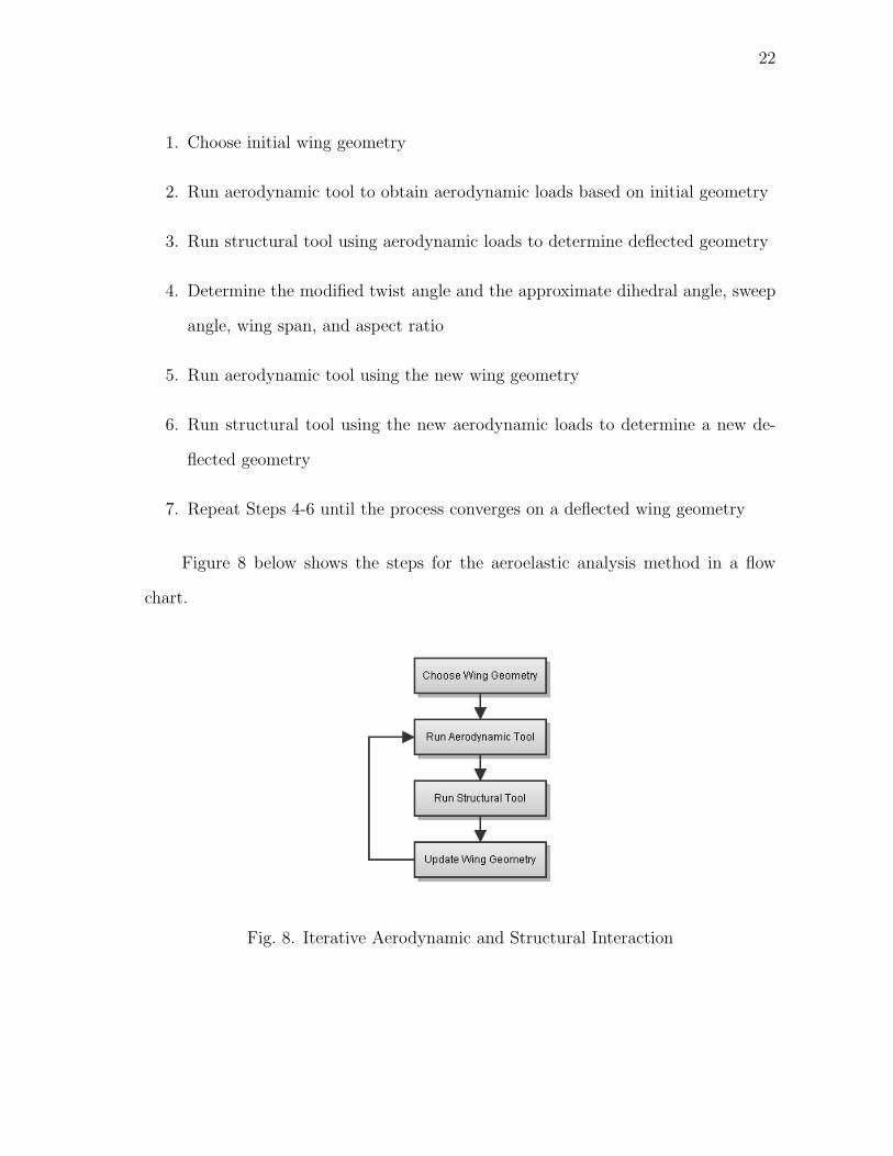
1. Choose initial wing geometry
2. Run aerodynamic tool to obtain aerodynamic loads based on initial geometry
3. Run structural tool using aerodynamic loads to determine deflected geometry
4. Determine the modified twist angle and the approximate dihedral angle, sweep
angle, wing span, and aspect ratio
5. Run aerodynamic tool using the new wing geometry
6. Run structural tool using the new aerodynamic loads to determine a new de-
flected geometry
7. Repeat Steps 4-6 until the process converges on a deflected wing geometry
The Figure 8 below shows the steps for the aeroelastic analysis method in a flow
chart.
Fig. 8. Iterative Aerodynamic and Structural Interaction

23
3. Contributions of This Research
This research is novel and represents a fundamental advance for several reasons. It
applies Finite Element Analysis to the morphing wing problem and uses an iterative
method to incorporate the aerodynamic and structural effects which is a unique ap-
proach for morphing applications. Also, this research develops the strucutral tool in a
way that allows it to easily interface with other existing morphing and Machine Learn-
ing tools. The use of the structural tool in morphing research is a new and unique
approach to learning about the structural impacts and limitations of a reconfigurable
wing.

24
CHAPTER II
FINITE ELEMENT ANALYSIS
This chapter will discuss the selection of the structural analysis method, derive the
necessary equations and theory, and discuss the limitations of the chosen approach.
A. Selection of Structural Analysis Method
Because a fully morphing aircraft can have an infinite number of wing configurations,
it would be too expensive and unrealistic to use the typical commercial finite element
tools which utilize 3-D modeling software. A new model would need to be created for
every different wing configuration. For this reason, a Finite Element Analysis (FEA)
code was selected as the most versatile tool for structural analysis of a morphing air
vehicle.
The major types of elements in FEA include beam, shell, and three-dimensional
brick elements. The beam model is the simplest because it reduces the structural
element to one independent spacial variable [28]. In order to simplify the problem,
a beam model of FEA was selected for the structural analysis method used in this
research. Linear and nonlinear analysis methods can be used for beam FEA. The
former is accurate if the material is in the linear elastic range and the changes in
geometry are small, and it is computationally simpler than nonlinear analysis. For
this reason, a linear analysis approach was selected for the FEA method used in the
research.
This chapter will discuss a specific type of linear beam FEA model known as
Space Frame Finite Element Analysis. A space frame is a structure with members
which may have any orientation in three dimensional space and may have forces
and moments in all directions at each elemental node, so there are six degrees of

25
freedom per node. A two-noded element is the simplest and most common type
of beam element, and with a two-noded element there will be nodal displacements
and rotations in all directions at either end of every element. It is possible to use
linear FEA to approximate the structural effects of a wing by modeling the wing as
a cantilevered beam that has small deflections assuming that the wing is an Euler-
Bernoulli beam, isotropic, and homogeneous. This means the cross-sections remain
planar and normal to the neutral axis, the properties are the same in all directions, and
there is a consistent material throughout. One of the limitations of Euler-Bernoulli
beam theory is that it is only accurate when modeling beams with a length to thickness
ratio of 15 to 1 or greater, where the thickness is in the direction of loading [30].
Unique dimensions, properties, and orientations for every element may be specified
to allow for the geometry of a morphed wing configuration.
B. Development of Finite Element Analysis Equations
This section discusses the theory of general FEA for space frames and shows the
derivation of the necessary equations. The approach follows methods and nomencla-
ture similar to that of Weaver in [25] and [27] as well as Haisler in [24].
1. Virtual Work Development of Finite Element Analysis
This subsection follows the methods shown in [25] . The generic displacements may
be defined within the element as the column vector u
u = {u, v, w, θx, θy, θz} (2.1)
where u, v, and w are the x, y, and z displacements, respectively. θ is the small
rotation about the axis shown in the subscript. θy and θz are the derivatives with

26
respect to x of w and v, respectively. The vector qe gives the displacements and
rotations at each node within the element. For a two-noded element, qe is given by
the following column vector
qe = {u1, v1, w1, θx1, θy1, θz1, u2, v2, w2, θx2, θy2, θz2} (2.2)
where the 1 and 2 subscripts denote the left and right nodes, respectively. The inter-
polation function or shape function, N, relates u and qe by the following equation.
u = Nqe (2.3)
The strain vector, ε, may be related to the displacements using a matrix d which is
a linear differential operator as shown below.
ε = du (2.4)
Substituting Equation 2.3 into 2.4 yields
ε = dNqe = Bqe (2.5)
where B is the matrix that gives the strains at any point in the element due to
the nodal displacements. The stress-strain relationship is defined using the following
equation
σ = Eε (2.6)
where E is the constitutive matrix relating the strains to the stress vector, σ. For
derivation purposes, the properties shown in this subsection, such as ε and E, in-
clude the full characteristics of a general structure and are vectors and matrices,
respectively. In the following subsection, these properties will be simplified using
assumptions which include small strain theory and Euler-Bernoulli beam theory.

27
The principle of virtual work states that the virtual work of external actions is
equal to the virtual strain energy of internal stresses for a structure in equilibrium
which is subjected to small virtual displacements. The following equation shows the
principle of virtual work for a finite element
δUe = δWe (2.7)
where δUe is the virtual strain energy due to internal stresses within an element and
δWe is the virtual work due to external forces on the element. Equation 2.3 may be
written in terms of virtual displacements as
δu = Nδqe (2.8)
Similarly, Equation 2.5 may be written in terms of virtual strains and displacements
as
δε = Bδqe (2.9)
The virtual strain energy may be written in terms of stress and strain as
δUe =∫VδεTσdV (2.10)
and the virtual work may be written in terms of the nodal boundary loads vector Pe
and distributed body loads vector f .
δWe = δqeTPe +
∫VδuT fdV (2.11)
By substituting Equations 2.10 and 2.11 into Equation 2.7, the following equation is
obtained: ∫VδεTσdV = δqe
TPe +∫VδuT fdV (2.12)
By manipulating Equation 2.12 with Equations 2.5, 2.6, 2.8, and 2.9, the following

28
equation is found: (∫V
BTEBdV)
qe = Pe +∫V
NT fdV (2.13)
which may be rewritten as
Keqe = Pe + Qe (2.14)
where Ke is the elemental stiffness matrix as shown below
Ke =∫V
BTEBdV (2.15)
and Qe is the vector of equivalent nodal loads due to the distributed loads vector as
seen below.
Qe =∫V
NT fdV (2.16)
2. Space Frame Stiffness Matrix and Equivalent Nodal Load Formulation
The approach in this section follows methods and nomenclature similar to that of
Weaver in [25]. Space Frame FEA uses beam elements which exhibit displacements
and rotations in any direction. Also, each element may have a unique local axis
orientation when compared to the neighboring elements. The elemental stiffness
matrices are determined by combining the stiffnesses which correspond to the axial,
flexural, and torsional elements.
An axial element is an element which may only experience u displacements due
to loads in the local x direction. The displacements may be assumed to vary linearly
with x within the element, and the following linear equation can be used to ensure
monotonic convergence of the solution:
u = c1 + c2x (2.17)
Using the element boundary conditions u (0) = q1 and u (L) = q7, where L is the

29
element length and the q1 and q7 correspond to indices 1 and 7 within Equation 2.2,
Equation 2.17 may be solved in terms of the interpolation function N as shown in
Equation 2.18
u = q1 +q7 − q1L
x =[1− x
L,x
L
] q1
q7
= Nqe, axial (2.18)
where
N =[1− x
L,x
L
](2.19)
B may be written as the derivative of N with respect to x for the axial element,
and E is the constant E, the elastic modulus which relates the axial stress and axial
strain. Using Equation 2.19 and the mentioned simplifications for B and E, Equation
2.15 may be written as the axial entries of the elemental stiffness matrix and shown
by the following equation
Ke, axial =∫ L
0EAx
dNj
dx
dNi
dxdx for i = 1, 7 and j = 1, 7 (2.20)
where Ax is the cross-sectional area which is perpendicular to the neutral axis of the
beam.
The flexural components of the elemental stiffness matrix may be developed
in a similar manner. A beam in bending experiences transverse displacements and
small rotations at each node. The assumed displacement function must be cubic to
account for the displacement and rotation boundary conditions at both x = 0 and
x = L. Considering bending about the z axis, the beam will have displacements,
v, and rotations, θz, which correspond to the indices 2, 6, 8, and 12 of the nodal
displacements and rotations given in Equation 2.2. The displacement function for
bending about the z axis which ensures monotonic convergence of the solution is

30
shown below.
v = c1 + c2x+ c3x2 + c4x
3 (2.21)
Using the boundary conditions to solve for the constants in Equation 2.21 as done
previously in 2.18, the following interpolation function for bending about the z axis
is found:
N =
[1− 3
x2
L2+ 2
x3
L3, x− 2
x2
L+x3
L2, 3
x2
L2− 2
x3
L3, −x
2
L+x3
L2
](2.22)
Because the flexural strain is a function of the curvature, or second derivative of v
with respect to x, Equation 2.15 may be written for the flexural components of the
stiffness matrix as follows:
Ke, flexural =∫ L
0EIz
d2Nj
dx2
d2Ni
dx2dx for i = 2, 6, 8, 12 and j = 2, 6, 8, 12 (2.23)
where
Iz =∫Ay2dA (2.24)
represents the moment of inertia about the z axis. For the case where the cross section
is a solid rectangle, Iz is defined as
Iz =bh3
12(2.25)
where b is the width along the z direction and h is the height along the y direction.
b is not the same as b which is used elsewhere in the thesis to refer to wing span.
Equation 2.26 gives Iz for a box cross section
Iz ≈bh3
12− (b− 2tw)(h− 2tf )
3
12(2.26)
where tw is the thickness of each of the two box sides which are perpendicular to the
z direction and tf is the thickness of the two sides perpendicular to the y direction.

31
The same method may be used to determine the flexural elemental stiffness
matrix for bending about the y axis, but w, θy, and Iy are used instead of v, θz, and
Iz, respectively. Iy is found for rectangular and box cross sections using Equations
2.27 and 2.28, respectively.
Iy =hb3
12(2.27)
Iy ≈hb3
12− (h− 2tf )(b− 2tw)3
12(2.28)
The indices of the stiffness matrix correspond to i = 3, 5, 9, 11 and j = 3, 5, 9, 11.
For a torsional element, there are only rotations θx about the x axis, so the
linear interpolation function in Equation 2.19 may be used. For pure torsion, E is
the constant G, the shear modulus of the material. For an isotropic material, G is
defined as
G =E
2(1 + ν)(2.29)
where ν is the Poisson’s ratio of the material. Equation 2.15 may be written as
Ke, torsional =∫ L
0GJ
dNj
dx
dNi
dxdx for i = 4, 10 and j = 4, 10 (2.30)
where J is the polar moment of inertia which is approximated as
J ≈ hb3[
1
3− 0.21
b
h
(1− b4
12h4
)](2.31)
for a solid rectangular cross section where h is greater than b. h and b must be
interchanged in Equation 2.31 if h is less than b. For a box cross section, Equation
2.32 is used to calculate J .
J ≈ [(h− tf )(b− tw)]2(tf + tw)
(b− tw) + (h− tf )(2.32)
The elemental stiffness matrix for elements experiencing axial, flexural, and tor-
sional deformations may be formed by combining the three stiffness matrices shown

32
in Equations 2.20, 2.23, and 2.30. The stiffness matrix is a twelve by twelve matrix
because there are six degrees of freedom for each of the two nodes. The matrix, Ke,
as shown by Weaver in [27], is presented in Equation 2.33.
The equivalent nodal loads for beam elements which experience axial, flexural,
and torsional deformations are found using Equation 2.16 with the interpolation func-
tions shown in Equations 2.19 and 2.22. Equation 2.34 gives the twelve by one column
vector for the elemental nodal loads. In Equation 2.34, f is the magnitude of the dis-
tributed force per length in the axis direction notated in the subscript and mx is the
distributed moment per length about the local x axis.
Ke =
EAxL
0 0 0 0 0 −EAxL
0 0 0 0 0
0 12EIzL3 0 0 0 6
EIzL2 0 −12
EIzL3 0 0 0 6
EIzL2
0 0 12EIy
L3 0 −6EIy
L2 0 0 0 −12EIy
L3 0 −6EIy
L2 0
0 0 0 GJL
0 0 0 0 0 −GJL
0 0
0 0 −6EIy
L2 0 4EIy
L0 0 0 6
EIy
L2 0 2EIy
L0
0 6EIzL2 0 0 0 4
EIzL
0 −6EIzL2 0 0 0 2
EIzL
−EAxL
0 0 0 0 0EAx
L0 0 0 0 0
0 −12EIzL3 0 0 0 −6
EIzL2 0 12
EIzL3 0 0 0 −6
EIzL2
0 0 −12EIy
L3 0 6EIy
L2 0 0 0 12EIy
L3 0 6EIy
L2 0
0 0 0 −GJL
0 0 0 0 0 GJL
0 0
0 0 −6EIy
L2 0 2EIy
L0 0 0 6
EIy
L2 0 4EIy
L0
0 6EIzL2 0 0 0 2
EIzL
0 −6EIzL2 0 0 0 4
EIzL
(2.33)

33
Qe =
12fxL
12fyL
12fzL
12mxL
− 112fzL
2
112fyL
2
12fxL
12fyL
12fzL
12mxL
112fzL
2
− 112fyL
2
(2.34)
3. Space Frame Axis Orientation and Transformation
The approach in this section follows methods and nomenclature similar to that of
Weaver in [27]. In the previous section, the equations for the elemental stiffness
matrix, Ke, and equivalent nodal loads, Qe, were developed with respect to the local
coordinate axes. In order to assemble all of the elements and analyze the entire
structure, each element must first be transformed into the global coordinate system.
The figure below, taken from [27], shows the orientation of the element with respect
to the global coordinates xs, ys, and zs. As shown in Figure 9, the local coordinate
axis must be rotated by angles α, β, and γ to transform the element into the global
coordinates. The following direction cosine matrices are utilized to transform the

34
Fig. 9. Rotation of Axes for a Space Frame Member [27]
coordinates about each rotation angle:
Rα =
1 0 0
0 cosα sinα
0 − sinα cosα
(2.35)
Rβ =
cos β 0 sin β
0 1 0
− sin β 0 cos β
(2.36)

35
Rγ =
cos γ sin γ 0
− sin γ cos γ 0
0 0 1
(2.37)
The negative sign occurs in Equation 2.36 in the lower left corner as opposed to the
upper right corner because β is a negative rotation about the yS axis shown in Figure
9. The rotation matrix may be formed by combining the direction cosine matrices
using the equation shown below.
R = RαRβRγ (2.38)
The elemental stiffness matrices and the equivalent nodal load vectors must be trans-
formed into the global coordinates. Ke is a twelve by twelve matrix and Qe is a
twelve by one vector, but Equation 2.38 yields a three by three matrix. The following
equation gives the necessary twelve by twelve rotation matrix:
RT =
R 0 0 0
0 R 0 0
0 0 R 0
0 0 0 R
(2.39)
The elemental stiffness matrix is transformed from the local coordinates to the global
coordinates using the equation
Ke, global = RTTKe, localRT (2.40)
and the elemental equivalent nodal loads vector is transformed using the equation
below.
Qe, global = RTTQe, local (2.41)

36
4. Assembly of the Global Stiffness Matrix and Solution
Once the elemental stiffness matrices and equivalent nodal loads are transformed
into the global coordinate system, the stiffness matrix and equivalent nodal loads for
the structure are assembled, the displacement and rotation boundary conditions are
applied, and the overall structure is analyzed. To develop the necessary equations,
the principle of virtual work for the structure, as described in [25], is shown below
δUs = δWs (2.42)
where the subscript s denotes that the term applies to the entire structure. Follow-
ing a similar approach as Subsection 1, the following equation relating the stiffness,
displacements, and loads for the overall structure is found:
Kq = P + Q (2.43)
where K is the assembled stiffness matrix for the structure, q is the nodal displace-
ment column vector for the structure, P is the column vector of external point loads
applied to nodes of the structure, and Q is the assembled equivalent nodal loads for
the structure.
The notation and methods shown below are similar to those used by Haisler in
[24]. To determine K, the Ke for every element must be combined. Because there are
six degrees of freedom per node and two nodes per element, the elemental stiffness
matrix may be subdivided into four quadrants with each quadrant consisting of a
six by six matrix. An example of the subdivided elemental stiffness matrix is shown
below
Ke1 =
K111 K12
1
K211 K22
1
(2.44)
where the subscripts denote the quadrant location and the superscript denotes the
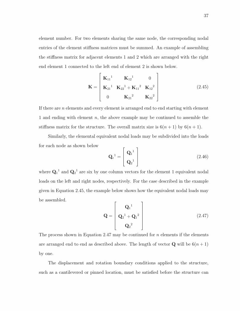
37
element number. For two elements sharing the same node, the corresponding nodal
entries of the element stiffness matrices must be summed. An example of assembling
the stiffness matrix for adjacent elements 1 and 2 which are arranged with the right
end element 1 connected to the left end of element 2 is shown below.
K =
K11
1 K121 0
K211 K22
1 + K112 K12
2
0 K212 K22
2
(2.45)
If there are n elements and every element is arranged end to end starting with element
1 and ending with element n, the above example may be continued to assemble the
stiffness matrix for the structure. The overall matrix size is 6(n+ 1) by 6(n+ 1).
Similarly, the elemental equivalent nodal loads may be subdivided into the loads
for each node as shown below
Qe1 =
Q11
Q21
(2.46)
where Q11 and Q2
1 are six by one column vectors for the element 1 equivalent nodal
loads on the left and right nodes, respectively. For the case described in the example
given in Equation 2.45, the example below shows how the equivalent nodal loads may
be assembled.
Q =
Q1
1
Q21 + Q1
2
Q22
(2.47)
The process shown in Equation 2.47 may be continued for n elements if the elements
are arranged end to end as described above. The length of vector Q will be 6(n+ 1)
by one.
The displacement and rotation boundary conditions applied to the structure,
such as a cantilevered or pinned location, must be satisfied before the structure can

38
be analyzed. One method of accounting for these restrictions is to add an extremely
large number to the assembled stiffness matrix indices which corresponds to the nodal
degree of freedom which is restricted. This method gives a nearly infinite stiffness
in the necessary degrees of freedom at the particular node. After K is modified to
account for the displacement and rotation boundary conditions, Equation 2.43 may
be solved for the vector q. The nodal displacements throughout the structure are
now known.
5. Post Processing and Axial Stress Analysis
Once the nodal displacements, q, are found for the structure, the individual elemental
nodal displacements, qe, are easily located within q in groupings of twelve. By using
the interpolation functions from Equations 2.19 and 2.22 with Equation 2.3, the
displacements and rotations throughout each element are found.
The elemental boundary loads are found by solving Equation 2.14 for Pe using
the newly found qe. In order to analyze the stresses within each element, the elemental
boundary forces must first be converted from the global coordinate system into the
local coordinates. The following equation may be used to transform the loads into
local system:
Pe, local = RTPe, global (2.48)
With the elemental boundary loads in the local coordinates, the following equa-
tion from Haisler in [24] may be used to determine the axial stress, σxx, throughout
the element:
σxx =P
Ax− Mzy
Izz+Myz
Iyy(2.49)
where y and z span across the height and width of the cross section, respectively,
in the local coordinate system with the origin located at the principal axis. P , My,

39
and Mz are terms within the vector Pe. Equations 2.48 and 2.49 may be used for
all elements to determine the internal loads and axial stresses throughout the entire
structure.
C. Assumptions
This chapter describes a linear beam FEA approach which contains many inherent
assumptions regarding the structural element. Because beam analysis is used, the x
dimension of each element must be significantly larger than the other two dimensions.
This means that the element must be long and slender. If the structure is composed
of elements which are arranged end to end as described above, then the elemental
geometric limitations become limitations of the overall structure. Because a linear
analysis method was selected, the displacements and rotations must be small when
compared to the overall size of the structure and the material cannot be highly flexible.
As described by Pai in [28], there are three types of beam theories: the Euler-
Bernoulli beam theory, the shear-deformable beam theories, and the three-dimensional
stress beam theories. The method used in this research is Euler-Bernoulli beam the-
ory, so only the axial stress, σxx, is considered and the cross sections are assumed
to remain plane and perpendicular to the reference axis after deformation. For the
flexural components, the transverse shear stresses and both in-plane and out-of-plane
warpings are neglected. For the torsional components, only the shear stresses are
considered. The Euler-Bernoulli approach accounts for only one of the six stress
states. The chosen method is accurate if the deflections and rotations are small and
the coupling effects between bending and twisting motion are insignificant.
By assuming the structure is composed of a homogeneous and isotropic material,
each element must have a uniform material throughout and the material properties

40
must be the same in all directions. This means that it is not possible to accurately
analyze a composite, anisotropic structure using the methods described in this chap-
ter. It should be noted that a beam model uses the cross-sectional area and moments
of inertia, but it does not model the actual shape of the cross section.
41
CHAPTER III
SPACE FRAME FINITE ELEMENT ANALYSIS
COMPUTATIONAL TOOL DEVELOPMENT
This chapter describes the implementation of the Space Frame Finite Element Anal-
ysis decribed in the previous chapter. The structural analysis computational tool
main program and subroutines are discussed. Flow charts are used throughout this
chapter to show the basic program operations. For a more detailed understanding of
the code operations, the full MATLAB code for the structural tool is included as a
supplemental file attached to this thesis.
A. Structural Tool Main Program
The organization of the structural tool main program, STRUCTURES, is shown in
flow chart form in Figure 10. The first set of inputs specifies the wing geometry and
loads. The geometry includes the wing span, aspect ratio, chord length taper ratio,
thickness taper ratio, root thickness as a percentage of the root chord length, root
incidence angle, tip incidence angle, leading edge sweep angle, and dihedral angle.
The chord taper ratio and thickness taper ratio, as shown by λchord and λthickness, are
the ratios of ct to cr and tt to tr, respectively.
The loads are input as a structure array which includes vectors of the lift, drag,
pitching moment, and load application coordinates. The individual element lengths
and node placement depend upon the load application coordinates. The program is
setup to analyze half of the wing at a time. If the left and right halves of the wing
are different, the program may be run twice, once for each half of the wing. The
coordinate axis was previously shown in Figure 9. Although aerodynamic loads are
distributed across the area of the wing, for this program they must be input as point

42
loads applied to the principal axis of the wing. A subroutine will later convert these
point loads into distributed loads over the length of each element. True point loads
may be included separately in the loads structure array. The weight is not included
as a load input because it will be calculated later using the material density.
Fig. 10. Structural Tool Main Program
The next set of inputs specifies whether the cross section type is a solid rectangle
or a box. If it is a box cross section, the box thicknesses th and tw must be included,

43
where th is the thickness of the top and bottom portions of the box cross section
and tw is the thickness of each side portion of the box cross section. The inputs also
include the material elastic modulus, shear modulus, and density. The units must
be specified as English or metric. Inches and pounds are used if English units are
selected and meters and Newtons are used for metric.
Because the tool is designed specifically for a wing, a cantilever constraint is
specified for the root of the wing. The final section of the main program includes all
of the subroutine calls.
B. Structural Tool Subroutines
This section describes all of the subroutines which are called by the structural tool
main program. The subroutines prepare the inputs for analysis, implement the equa-
tions given in the previous chapter, and display the structural analysis results.
1. Setup Subroutines
The subroutines described in this subsection, manipulate the inputs so that the struc-
ture may be analyzed. The first subroutine is GEOMETRY, and it is shown in Figure
11. GEOMETRY first calculates the number of elements, n. It next determines the
global coordinates and incidence angle at each node and calculates the wing area and
the chord and thickness lengths at the root and tip. Finally, the subroutine creates a
structure array called element for any properties specific to individual elements. The
height, width, and incidence angle are calculated for each element.
The next subroutine is called MODIFY INPUTS. This subroutine assigns the
inputs for E, G, ρ, and the box cross section thicknesses to each element. This
subroutine exists in case the material properties change for different sections of the

44
Fig. 11. GEOMETRY Subroutine
wing. The MODIFY INPUTS subroutine is shown in Figure 12.
The PRINT VALUES subroutine prints each of the inputs to an output file.
Its flow chart has been omitted because it is simple and is not necessary for the
functioning of the overall program.
The next subroutine is ELEMENT VALUES, and it is shown in Figure 13. This
subroutine calculates the Ax, J , Iyy, and Izz for each element for the rectangular solid
or box cross section types. Using the nodal coordinates, the element length, L, and
direction cosines, Cx, Cy, Cz, are calculated. From the direction cosines, the β and γ
rotation angles are found for each element. This process is described in [27].
2. Analysis Subroutines
The next set of subroutines implements many of the equations specified in the previous
chapter. These subroutines assemble the stiffness matrix for the structure, impose

45
Fig. 12. MODIFY INPUTS Subroutine
the constraints, assemble the equivalent nodal loads and point loads, then solve the
system of equations to determine the nodal displacements.
The first subroutine discussed in this subsection is ASSEMBLE K. The flow chart
for ASSEMBLE K is shown in Figure 14. First, Equation 2.33 is used and the local
elemental stiffness matrices are calculated. Next, the elemental rotation matrices are
found using Equations 2.35 - 2.39. Using Equation 2.40, the local elemental stiffness
matrices are converted to the global coordinates. Finally, the stiffness matrix for
the structure is assembled as described in Equation 2.45. For more details on how
this process is implemented, see the subroutine code included in structural tool code
which is attached as a supplemental file to this thesis.

46
Fig. 13. ELEMENT VALUES Subroutine
The IMPOSE CONSTRAINTS subroutine is not shown because it is fairly sim-
ple. It adds a value of 1030 to the indices of the stiffness matrix which correspond
to the degrees of freedom constrained by the displacement and rotation boundary

47
Fig. 14. ASSEMBLE K Subroutine
conditions.
The next subroutine is ASSEMBLE Q, and it is shown in Figure 15. As pre-
viously mentioned, the aerodynamic loads are input as point loads and need to be
converted to loads distributed over the length of each element. First this subroutine
uses the units value to determine the gravitational acceleration constant, g. Using
g, ρ, and the lift force, the distributed load fy is calculated for each element. From
the drag force and pitching moment, fz and mx are calculated for each element. fy,
fz, and mx are then used in Equation 2.34 to determine the equivalent nodal loads

48
for each element. The equivalent nodal loads for the structure are then assembled
following the method described by Equation 2.47.
Fig. 15. ASSEMBLE Q Subroutine

49
The final two subroutines of the Analysis subsection are the ASSEMBLE P and
SOLVER subroutines. The flow charts for these subroutines are omitted because
they are both very simple. ASSEMBLE P takes the point loads specified at specific
nodes in the loads structure array and includes them in the full point load vector
P. The SOLVER subroutine uses K, Q, and P to solve Equation 2.43 for the nodal
displacements q.
3. Post Processing Subroutines
This subsection describes the subroutines related to the generation of figures showing
the displacements, rotations, and axial stress throughout the structure. Most of the
flow charts shown in this subsection are very simplified when compared to the actual
code. See attached structural tool code for the full details.
The first subroutine is PLOT DEFLECTION which is shown in Figure 16. The
subroutine first finds the individual elemental nodal displacement vectors, qe, from
the full vector q. Next, the interpolation functions are found using Equations 2.19
and 2.22. Equation 2.3 uses qe and the interpolation functions to calculate the dis-
placements and rotations throughout each element. The elemental rotation matrix
must be used to determine the torsional rotations in the local coordinates. Adding
the displacements and rotations to the original wing coordinates gives the deflected
wing geometry. Finally, the subroutine generates plots of v, y, w, z, and θx versus x.
The next subroutine is PLOT DEFLECTION 3D, and it is shown in Figure 17.
This subroutine generates a three dimensional wire-frame view of the deflected struc-
ture. Because Space Frame FEA only models the deflections of the principal axis,
the principal axis is also plotted. The deflections and rotations are very small and
will not be observed when the entire structure is shown, so the subroutine uses dis-
placement and rotation scale factors. The displacements and rotations are multiplied

50
by the scale factors and then used with the element lengths, widths, heights, and
axis rotation angles to determine the 3D geometry. The edges of the structure, the
connecting lines at the ends of each element, and the principal axis are plotted.
Fig. 16. PLOT DEFLECTION Subroutine

51
Fig. 17. PLOT DEFLECTION 3D Subroutine
The STRESS subroutine calculates the axial stress along the principal axis at
each node and generates a plot of σxx versus x. The flow chart for the STRESS
subroutine is shown in Figure 18. In order to calculate the axial stress, Pe must first
be determined by solving Equation 2.14. Next, Equation 2.48 is used to convert Pe
from the global to the local coordinates of each element. Then Equation 2.49 is used

52
to calculate σxx at each node along the principal axis. At the principal axis, the local
y and z coordinates are 0, so the second and third terms of Equation 2.49 are both
0. Finally the subroutine plots σxx versus x for the entire structure.
Fig. 18. STRESS Subroutine
The final subroutine, PLOT STRESS 3D, generates a three dimensional surface
plot of the axial stress and is shown in Figure 19. Using Equation 2.49, the axial stress
is found at corners of the cross section at incremental spaces within each element.
Next, matrices of the global x, y, and z coordinates and corresponding σxx are found
for each of the six surfaces of the rectangular solid represented by the analysis. Surface
plots of the axial stress are then made for each of the surfaces.

53
Fig. 19. PLOT STRESS 3D Subroutine

54
CHAPTER IV
SPACE FRAME FINITE ELEMENT ANALYSIS
COMPUTATIONAL TOOL
VALIDATION AND VERIFICATION
The purpose of this chapter is to demonstrate that the structural tool is working
correctly and may be applied to the morphing wing problem. The first section will
validate the tool using the same method of linear beam FEA in Abaqus. The sec-
ond section will use several more complex FEA models in Abaqus to show that the
structural tool is a realistic approach.
A. Validation
The goal of this section is to demonstrate that the Space Frame FEA structural tool
yields physically correct results. The structural analysis program Abaqus is used to
generate comparison cases for the Space Frame FEA using the same type of finite
element model.
1. Case Description
Because the tools developed from this research will primarily be used in development
of Micro Air Vehicles and other small scale RC aircraft, similar scale and material
properties as the Texas A&M University Manureva RC aircraft wing design project
are used for each validation and verification case. More details for the Manureva
aircraft are described in Reference [29] and in a later section. The Table I describes
the properties used for the validation case. The material properties shown are those of
Basswood, which was the material used for the spar caps of the Manureva. Although
wood is an orthotropic material, isotropic properties are assumed. A Poisson’s ratio

55
Table I. Validation Case
Parameter Value
b (in) 80
AR 10
Λ (deg) 0
Γ (deg) 0
cr & ct (in) 8
tr & tt (%c) 0.12
αr & αt (deg) 0
Ebasswood (psi) 1.537E6
of 0.3 is used for all materials in this chapter.
The structural tool and Abaqus models both contain the right half-span of the
wing with a cantilever boundary condition at the wing root. When Abaqus and the
structural tool are compared, both models contain the same cross sectional properties.
The Abaqus analysis uses the same linear FEA method and Euler-Bernoulli beam
model, so the results should match exactly.
Two different cross section cases are evaluated: a solid cross section and a box
cross section with 1/8 inch thick walls. The dimensions of the cross sections corre-
spond to the chord length and wing thickness for a wing with zero sweep and zero
dihedral. The moments of inertia are described for solid and box cross sections in
Equations 2.25, 2.26, 2.27, and 2.28 and the polar moments of inertia are shown in
Equations 2.31 and 2.32. For each cross section case, two different load cases are used
for the validation: pure lift and pure torsion. The Manureva aircraft had a 3g lift
load of 22.5 lbs for the half span, so the same load was distributed equally over the

56
beam model of the wing. The pure torsion case uses a pitching moment of 10 in-lbs
applied to the wing tip.
2. Solid Cross Section Case
The Figure 20 shows the y displacements, v, for the case of pure bending due to lift for
the solid cross section. As shown in Figure 20, the deflections for Abaqus matched
0 5 10 15 20 25 30 35 400
0.02
0.04
0.06
0.08
0.1
0.12
0.14
0.16
0.18
0.2
Span (in)
Y D
efle
ctio
n (in
)
CodeAbaqus Linear Beam Analysis
Fig. 20. Linear Euler-Bernoulli Analysis, Deflection due to Lift, Basswood Solid Cross
Section
with those generated by the structural tool. The difference between the values is
much less than 0.1%, as show in Table II. Figures 21 and 22 show the axial stress for
the pure lift load case as generated by Abaqus and the structural tool, respectively.
A visual comparison of Figures 21 and 22 shows that the values in the two plots
are very close, and an actual numerical comparison of the values at the lower corner
nodes of the wing root demonstrates that Abaqus and the structural tool give results
within 0.0106%. It should be noted that the three dimensionality of Figure 22 is a
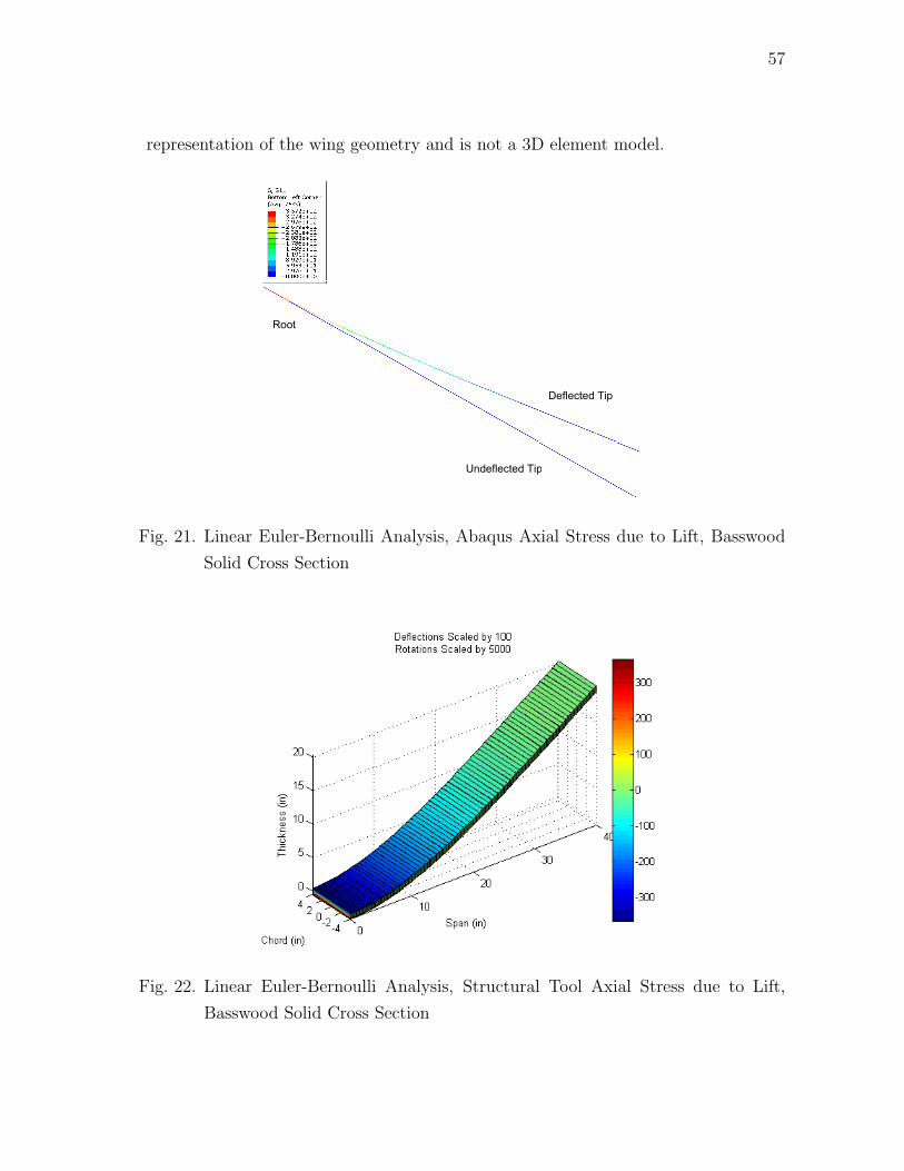
57
representation of the wing geometry and is not a 3D element model.
Deflected Tip
Undeflected Tip
Root
Fig. 21. Linear Euler-Bernoulli Analysis, Abaqus Axial Stress due to Lift, Basswood
Solid Cross Section
Fig. 22. Linear Euler-Bernoulli Analysis, Structural Tool Axial Stress due to Lift,
Basswood Solid Cross Section

58
Table II. Structural Tool Accuracy Compared to Abaqus Results
Analysis Beam Type Material Cross Deflection Rotation
Type Section Accuracy Accuracy
Linear Euler-Bernoulli Basswood Solid 5.89E-5% 0.280%
Linear Euler-Bernoulli Basswood Box 0.942% 1.11E-5%
Linear Timoshenko Basswood Solid 0.571% 0.280%
Linear Timoshenko Basswood Box 2.97% 1.11E-5%
Linear Timoshenko Balsa Box 2.97% 0.0369%
Nonlinear Timoshenko Basswood Solid 0.569% 0.280%
Nonlinear Timoshenko Balsa Box 2.59% 0.0775%
Figure 23 shows the rotations, θx, due to the pitching moment for the pure torsion
load case. The comparison shows that the Abaqus and structural tool give results
within 0.280% as shown in Table II.
3. Box Cross Section Case
This subsection uses the same load cases and wing properties as the analysis described
in the previous section, except the cross section is a box with 1/8 inch thick walls.
Figure 24 shows the displacements for the pure lift case and Figure 25 shows the
rotations for the pure torsion case. Figures 24 and 25 both demonstrate that the
structural tool gives very accurate results when compared to Abaqus for the box
cross section case. The accuracy for these cases is also shown in Table II.
The validation shows that the structural tool and Abaqus give very similar results
for all cross section and load cases. Several other tests were also used to validate the
structural tool. By using a symmetric cross section beam, a pure lift case and pure
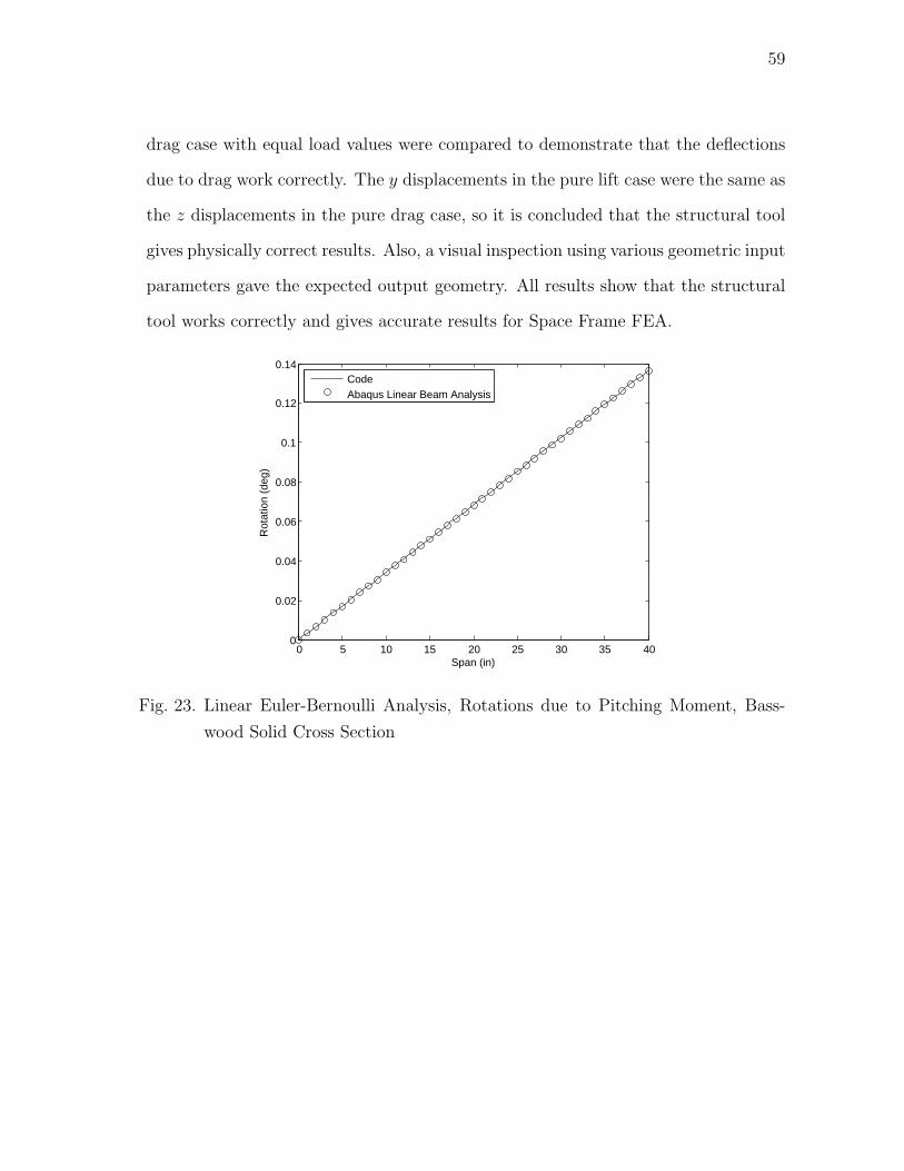
59
drag case with equal load values were compared to demonstrate that the deflections
due to drag work correctly. The y displacements in the pure lift case were the same as
the z displacements in the pure drag case, so it is concluded that the structural tool
gives physically correct results. Also, a visual inspection using various geometric input
parameters gave the expected output geometry. All results show that the structural
tool works correctly and gives accurate results for Space Frame FEA.
0 5 10 15 20 25 30 35 400
0.02
0.04
0.06
0.08
0.1
0.12
0.14
Span (in)
Rot
atio
n (d
eg)
CodeAbaqus Linear Beam Analysis
Fig. 23. Linear Euler-Bernoulli Analysis, Rotations due to Pitching Moment, Bass-
wood Solid Cross Section

60
0 5 10 15 20 25 30 35 400
0.05
0.1
0.15
0.2
0.25
0.3
0.35
Span (in)
Y D
efle
ctio
n (in
)
CodeAbaqus Linear Beam Analysis
Fig. 24. Linear Euler-Bernoulli Analysis, Deflections due to Lift, Basswood Box Cross
Section
0 5 10 15 20 25 30 35 400
0.05
0.1
0.15
0.2
0.25
Span (in)
Rot
atio
n (d
eg)
CodeAbaqus Linear Beam Analysis
Fig. 25. Linear Euler-Bernoulli Analysis, Rotations due to Pitching Moment, Bass-
wood Box Cross Section

61
B. Verification
This section compares the Space Frame FEA structural tool with various types of
FEA models generated by Abaqus. Each Abaqus model is more complex and more
accurate than the structural tool. The following types of Abaqus models are used in
the verification: Timoshenko linear beam model, Timoshenko nonlinear beam model,
3D brick model, and the Manureva wing model. The material and cross sectional
properties are the same for the structural tool and Abaqus models for the Timoshenko
and 3D brick modesls, but are different for the Manureva wing model. The objective
of this section is to demonstrate that the structural tool accurately generates results
to a problem with a known solution.
1. Timoshenko Linear Beam Model
Timoshenko beam theory is more accurate than Euler-Bernoulli beam theory because
it accounts for shear deformations. It is also capable of modeling shorter beams than
Euler-Bernoulli beam theory. The structural tool is compared to the Timoshenko
model for the geometry parameters described in Table I in the Validation section.
Figure 26 shows displacements for the pure lift case with solid cross section as
described in the Validation section. As shown in Figure 26, the structural tool gives
results within 0.571% when compared to the Timoshenko beam model for the solid
cross section. The pure torsion case also gives very accurate results for the solid cross
section as shown in Table II.
The shear deformation effects are slightly more prominent in the box cross section
deflection case. Figure 27 shows the displacements due to the pure lift case for the box
cross section described in the previous section. The differences between Timoshenko
and structural tool deflections are noticeable in Figure 27, but the difference of 0.01

62
0 5 10 15 20 25 30 35 400
0.02
0.04
0.06
0.08
0.1
0.12
0.14
0.16
0.18
0.2
Span (in)
Y D
efle
ctio
n (in
)
CodeAbaqus Linear Beam Analysis
Fig. 26. Linear Timoshenko Analysis, Deflections due to Lift, Basswood Solid Cross
Section
inches in the tip deflection is within 2.97% and is very small when compared to the
wing half-span of 40 inches. The rotations in the pure torsion case for the box cross
section matched closely for the Timoshenko model and the structural tool.
1/8 inch balsa was also used for box cross section with the same load cases.
The material properties selected for balsa are an elastic modulus of 1.853E5 psi and
a Poisson’s ratio of 0.3. The deflection and rotation accuracy for the balsa case is
shown in Table II. The Timoshenko linear beam model shows that the structural tool
is very accurate for the given wing geometry.
2. Timoshenko Nonlinear Beam Model
Nonlinear analysis uses an iterative method to solve for the deflected wing geometry,
and it is more accurate than linear analysis when the deflections become large. For
the case described in Table I, Timoshenko nonlinear beam analysis is compared to

63
0 5 10 15 20 25 30 35 400
0.05
0.1
0.15
0.2
0.25
0.3
0.35
Span (in)
Y D
efle
ctio
n (in
)
CodeAbaqus Linear Beam Analysis
Fig. 27. Linear Timoshenko Analysis, Deflections due to Lift, Basswood Box Cross
Section
the structural tool. Figures 28 and 29 show the deflections for the pure lift case
and the rotations for the pure torsion case for the solid cross section. As shown
in Figures 28 and 29, the structural tool gives results accurate within 0.569% and
0.280%, respectively, when compared to the nonlinear analysis for the basswood solid
cross section.
Next, a more flexible structure was modeled in Abaqus using a box cross section
with balsa as the material. The results are shown in Figure 30. The accuracy of
the structural tool when compared to the nonlinear Timoshenko beam analysis is
very close to the accuracy when compared to the linear Timoshenko beam analysis
as shown in Table II. The results for the nonlinear beam analysis show that the
structural tool is very accurate for the given material properties and loads. If the
deflections become much larger due to either loads higher than the 3g case or the
use of a much more flexible material than basswood or balsa, then nonlinear analysis

64
may be necessary.
0 5 10 15 20 25 30 35 400
0.02
0.04
0.06
0.08
0.1
0.12
0.14
0.16
0.18
0.2
Span (in)
Y D
efle
ctio
n (in
)
CodeAbaqus Nonlinear Beam Analysis
Fig. 28. Nonlinear Timoshenko Analysis, Deflections due to Lift, Basswood Solid Cross
Section
0 5 10 15 20 25 30 35 400
0.02
0.04
0.06
0.08
0.1
0.12
0.14
Span (in)
Rot
atio
n (d
eg)
CodeAbaqus Nonlinear Beam Analysis
Fig. 29. Nonlinear Timoshenko Analysis, Rotations due to Pitching Moment, Bass-
wood Solid Cross Section

65
0 5 10 15 20 25 30 35 400
0.5
1
1.5
2
2.5
3
Span (in)
Y D
efle
ctio
n (in
)
CodeAbaqus Analysis
Fig. 30. Nonlinear Timoshenko Analysis, Deflections due to Lift, Balsa Box Cross
Section
3. 3D Brick Model
The next method of verification uses 3D brick finite elements to model the wing in
Abaqus. The objective is to observe the performance of the structural tool for various
sweep angles when the load case consists of simultaneous lift and pitching moment
loads. An example of the right half-span wing Abaqus model at a 30 degree sweep
angle is shown in Figure 31.
The wing structure uses the solid rectangular cross section with the basswood
material as described in previous sections. In Abaqus, 60% of the 22.5 lb load is
distributed over the area of the forward half of the wing and 40% is distributed
over the area of the aft half. The structural tool uses the equivalent lift force and
pitching moment distributed over the length of the principal axis. The cases used for
comparison consist of sweep angles ranging from 0 degrees to 50 degrees, changing
by 10 degree increments. Table III shows the comparison between to structural tool

66
and Abaqus model wing tip deflections and rotations for each sweep case. It also
compares the maximum axial stress at the wing root.
Table III. Structural Tool and Abaqus Model Results for Varying Sweep Angles
Model Sweep Tip Tip Root Maximum
Angle (deg) Deflection (in) Rotation (deg) Axial Stress (psi)
Abaqus 0 0.262 0.0623 274.4
Structural Tool 0 0.199 0.0615 366.2
Abaqus 10 0.277 −0.00630 283.0
Structural Tool 10 0.213 0.0624 382.1
Abaqus 20 0.329 −0.0959 315.7
Structural Tool 20 0.269 0.0655 438.7
Abaqus 30 0.447 −0.243 380.7
Structural Tool 30 0.404 0.0714 559.6
Abaqus 40 0.711 −0.528 561.7
Structural Tool 40 0.745 0.0812 808.4
Abaqus 50 1.40 −1.18 911.9
Structural Tool 50 1.79 0.0973 1369.9

67
Tip
Root
Fig. 31. Abaqus 3D Brick Element Model, 30 Degree Sweep Angle, Axial Stress
0 5 10 15 20 25 30 35 40 45 500
0.2
0.4
0.6
0.8
1
1.2
1.4
1.6
1.8
Sweep Angle (deg)
Tip
Def
lect
ion
(in)
Structural ToolAbaqus Analysis
Fig. 32. 3D Brick Element and Structural Tool Comparison for Deflection with Sweep
The values in Table III for tip deflection, tip rotation, and maximum root axial
stress are compared to the sweep angle in Figures 32, 33, and 34, respectively. As
shown in Figure 32, the structural tool under predicts the tip deflections at the low

68
0 5 10 15 20 25 30 35 40 45 50−1.2
−1
−0.8
−0.6
−0.4
−0.2
0
0.2
Sweep Angle (deg)
Tip
Rot
atio
n (d
eg)
Structural ToolAbaqus Analysis
Fig. 33. 3D Brick Element and Structural Tool Comparison for Rotation with Sweep
sweep angles, and it over predicts the tip deflection beginning near 40 degrees sweep.
Figure 33 shows the rotations are very accurate when comparing the two models
for the unswept case, but they are very different for the swept cases. The rotation
angle is calculated for the Abaqus model using the displacements at the leading and
trailing edge wing tip corners. The coupled bending and torsional effects due to sweep
and the combined forces and moments create a very complex interaction. A likely
reason the rotations are very different in the two models is the elastic axis location
in the structural tool model is selected to be on the mid-chord line of the wing. In
reality the elastic axis is typically forward of the mid-chord line for a swept wing.
Another possible reason the rotations are different is the wing planform shape at the
wing tip is different for each of the models. Because the wing planform is modeled as
a parallelogram shape in Abaqus, the area near the trailing edge corner of the wing
tip is smaller than the area near the leading edge corner for the swept cases. The

69
0 5 10 15 20 25 30 35 40 45 50200
400
600
800
1000
1200
1400
Sweep Angle (deg)
Max
imum
Roo
t Axi
al S
tres
s (p
si)
Structural ToolAbaqus Analysis
Fig. 34. 3D Brick Element and Structural Tool Comparison for Deflection with Sweep
smaller area near the trailing edge corner may be the reason the trailing edge tip has
higher deflections than the leading edge even though aft section loads are smaller.
The result is a negative rotation angle for the 3D element model, while the structural
tool yields a positive angle for all sweep cases. More investigation of the differences
between the 3D element model and beam model is required in order to understand
the rotation discrepancy.
When comparing the axial stress in Figure 34, the structural tool over predicts
the stress in all sweep angle cases. The major difference between the two models
is the cantilever boundary condition at the wing root. For the Abaqus model, the
boundary condition is the same for all cases because the shape of the wing planform is
a parallelogram. The structural tool models the principal axis for a rectangular wing
planform, and the cantilever boundary condition effectively rotates with the wing as it
is swept. Because the geometry of the structural tool and Abaqus models are slightly

70
different, the structural tool does not fully account for the boundary conditions. As
shown in Figure 31, the Abaqus models shows higher stress concentrations near the
trailing edge root than the leading edge root for the 30 degree sweep case. The
structural tool model, shown in Figure 35, shows fairly uniform stress across the wing
root.
Fig. 35. Structural Tool, 30 Degree Sweep Angle, Axial Stress
Although the structural tool predicts somewhat different results than the Abaqus
3D brick element models, the tool still gives reasonable results in certain cases. In
the case of the deflections, the tool predicts results within 0.1 inches from the Abaqus
values for all sweep angles less than 50 degrees. This difference in deflections is still
extremely small considering the wingspan is 80 inches. The rotation angles were
very different for the swept cases, so more investigation of the complex bending and
torsion interaction is required to determine the validity of the structural tool. When
comparing the axial stresses, the structural tool typically over predicted the stress
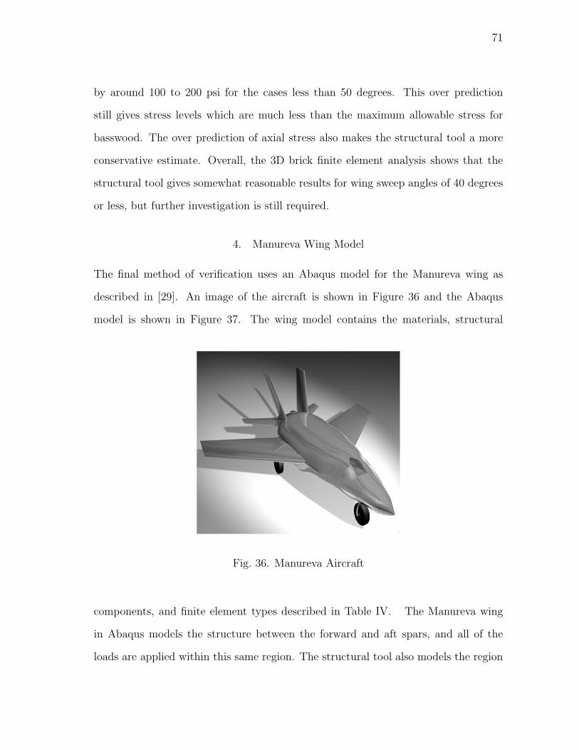
71
by around 100 to 200 psi for the cases less than 50 degrees. This over prediction
still gives stress levels which are much less than the maximum allowable stress for
basswood. The over prediction of axial stress also makes the structural tool a more
conservative estimate. Overall, the 3D brick finite element analysis shows that the
structural tool gives somewhat reasonable results for wing sweep angles of 40 degrees
or less, but further investigation is still required.
4. Manureva Wing Model
The final method of verification uses an Abaqus model for the Manureva wing as
described in [29]. An image of the aircraft is shown in Figure 36 and the Abaqus
model is shown in Figure 37. The wing model contains the materials, structural
Fig. 36. Manureva Aircraft
components, and finite element types described in Table IV. The Manureva wing
in Abaqus models the structure between the forward and aft spars, and all of the
loads are applied within this same region. The structural tool also models the region

72
Table IV. Manureva Abaqus Model Structural Components
Elastic Thickness Structural Element
Material Modulus (psi) (inches) Component Type
Basswood 1.537E6 3/8 Spar Caps 3D Brick
Balsa 1.853E5 1/8 Spar Shear Webs 3D Brick
Plywood 1.8E6 1/8 Ribs, Carry-Through Structure 3D Brick
Monokote 5.0E4 0.01 Skin Shell
between the forward and aft spars, as opposed to the entire wing, in order to accu-
rately approximate the Abaqus model. Table V shows the wing geometric parameters
modeled by the structural tool.
The 3g lift loads for the half-span Manureva wing are applied in Abaqus, and
they are distributed to each of the wing ribs using point loads applied near the forward
and aft spars. 65% of the load is applied to the portion of each rib near the forward
spar, and 35% is applied to the portion of each rib near rear spar. To represent the
equivalent loads in the structural tool, the lift loads are moved to the principal axis
and the corresponding pitching moments are applied. Because the loads which are
applied near the forward spar give positive moments and those near the aft spar give
negative moments, adjacent positive and negative moments are combined. Table VI
shows the loads applied in the structural tool.
The Abaqus wing model is more complex than the structural tool. The structural
tool uses either a solid rectangular cross section or a rectangular box cross section
where as the Abaqus model uses various structural components such as ribs, spar caps,
spar shear webs, skin, and a wing carry-through structure. Also, the structural tool

73
Printed using Abaqus/CAE on: Sat May 29 16:26:02 Central Daylight Time 2010
Fig. 37. Manureva Wing Abaqus Deflections
uses only one material and beam finite elements, and the Abaqus model uses various
materials and 3D brick elements and shell elements. The boundary conditions for the
wing carry-through structure in Abaqus are also more complex than a cantilevered
beam. These differences mean that the structural analysis results will be different.
The y displacements throughout the Manureva Abaqus wing model are shown
in Figure 37. For the first attempt to model the wing using the structural tool,
a box cross section with 1/8 inch basswood was selected. As shown in Figure 38,
the basswood is much too stiff. This is to be expected because the Abaqus wing
model does not contain nearly as much stiff material as a basswood box cross section.
1/8 inch Balsa was used as the next material and is also shown in Figure 38. The
balsa tip deflection is higher than the Abaqus model tip deflection, but the boundary
conditions for the Abaqus and structural tool models are also different.
In Abaqus, displacement constraint boundary conditions are applied to the top
surface of the forward and aft members of the wing carry-through structure. Figure 39
shows the 1/8 inch balsa structural tool plots with various boundary conditions. One

74
Table V. Manureva Wing Structure Geometry Parameters
Parameter Value
b (in) 74.4
AR 10
Λ (deg) 30.8
Γ (deg) 0
cr (in) 9.2
λchord 0.61
tr (%c) 0.27
λthickness 0.44
αr & αt (deg) 0
of the plots has the cantilever constraint at 0 inches, and this is the same plot shown in
Figure 38. Another structural tool plot shown in Figure 39 has a cantilever boundary
condition at the edge of the wing carry-through structure which occurs at 9 inches in
the span direction. The 9 inch cantilever location leads to an under approximation
of the tip displacement shown in the Abaqus model, so the most realistic location for
the cantilever position is somewhere between 0 and 9 inches. Using 3 inches as the
location for the boundary condition gives an accurate approximation within 7.10% of
the deflections found in Abaqus, as shown in Figure 39.
Comparing the wing tip rotations, the Abaqus model gave rotations of 0.48 de-
grees where as the structural tool gave 0.16 degrees. The rotations for structural tool
are smaller because the balsa along the upper and lower surfaces is more restrictive
to the rotations than the monokote skin used in the Abaqus model.
The axial stress within the wing may also be compared between the Abaqus and

75
Table VI. Structural Tool Manureva Loads
Lift (lbs) Span Location (in) Pitching Moment (in-lbs) Span Location (in)
1.46 37.2 3.6 37.2
0.79 34.5 5.0 33.4
2.56 32.2 5.7 28.1
1.38 29.0 3.5 22.8
3.29 27.2 2.7 17.7
1.77 23.7 3.3 12.5
3.29 21.8
1.77 18.4
2.56 17.1
1.38 13.0
2.25 12.0

76
0 5 10 15 20 25 30 35 40−0.1
0
0.1
0.2
0.3
0.4
0.5
0.6
0.7
Span (in)
Y D
efle
ctio
n (in
)
Abaqus AnalysisStructural Tool BasswoodStructural Tool Balsa
Fig. 38. Manureva Wing Deflections, Material Comparison
structural tool models. Figures 40 and 41 show the axial stress for the Abaqus and
structural tool models, respectively. Because the two structures are very different, it
is very difficult to compare the axial stresses. The high stress concentrations in the
Abaqus model occur in places where the area is very small which are not present in
the box structure. In general, the axial stress results found using the structural tool
are on the same scale as the Abaqus results for the majority of the wing and give an
acceptable approximation.
Modeling the Manureva wing structure using the structural tool does not give a
perfect representation of the wing structure, but it gives a reasonable approximation.
Overall, the verification shows that the structural tool provides adequate results and
is a valid tool for use in future morphing research.
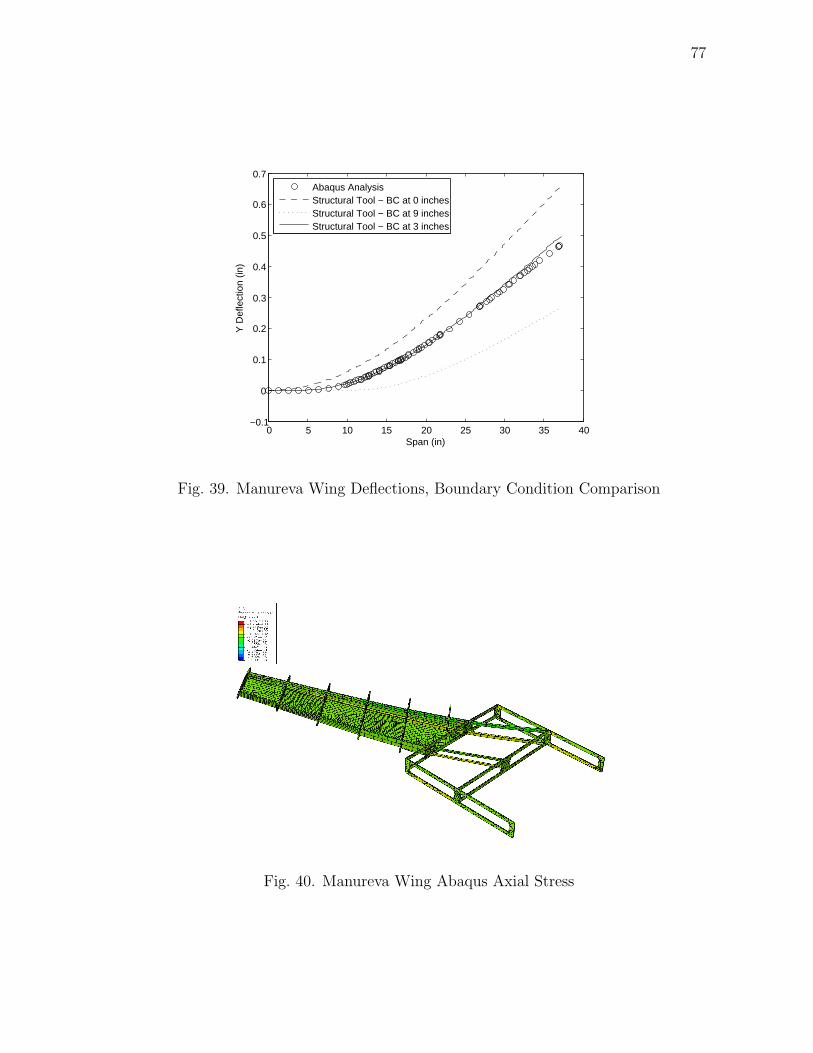
77
0 5 10 15 20 25 30 35 40−0.1
0
0.1
0.2
0.3
0.4
0.5
0.6
0.7
Span (in)
Y D
efle
ctio
n (in
)
Abaqus AnalysisStructural Tool − BC at 0 inchesStructural Tool − BC at 9 inchesStructural Tool − BC at 3 inches
Fig. 39. Manureva Wing Deflections, Boundary Condition Comparison
Printed using Abaqus/CAE on: Sat May 29 16:08:41 Central Daylight Time 2010
Fig. 40. Manureva Wing Abaqus Axial Stress

78
Fig. 41. Manureva Wing Structural Tool Axial Stress

79
CHAPTER V
ITERATIVE QUASI-STATIC AEROELASTIC ANALYSIS
This chapter discusses the interaction between the aerodynamic and structural tools
and presents the quasi-static aeroelastic results.
A. Aerodynamic Tool
This section describes the capabilities and limitations of an aerodynamic tool used
for morphing analysis by the Texas A&M University Vehicle Simulation & Control
Laboratory. This tool was developed externally to this thesis and is described in in
more detail in References [1] and [2]. The aerodynamic tool uses a constant strength
doublet-source panel method. The tool assumes that the air flow is incompressible
and inviscid, so it is valid for speeds less than Mach 0.3 and while in the linear range of
angle-of-attack. It is nominally set to use 130 chordwise panels and 25 spanwise panels
for the half-span and is capable of modeling a wing with the morphing parameters
described in Chapter I. It models NACA 4-Digit Series airfoil cross sections at the
wing root and the left and right wing tips. One limitation of the tool is that it is not
programmed to model deflected wing geometries.
The tool uses wing geometry and flight condition inputs and produces the aero-
dynamic coefficients, CL, CD, and CM , for the wing. CL is calculated by summing
the lift coefficients from every panel. CD is computed using the parabolic drag polar
CD = CD0 +CL
2
πeAR(5.1)
where the parasite drag coefficient, CD0, is found using an approximation based on
the wing area, wetted area, and correlation coefficients related to the equivalent skin
friction. In Equation 5.1, the second term is known as the induced drag and depends

80
on the coefficient of lift, and e is the Oswald efficiency factor. The pitching moment
coefficient, CM , is calculated by summing the moment coefficient due to the lift coeffi-
cient at each panel. The moment arm used to calculate the panel moment coefficients
is the longitudinal distance from the panel to the leading edge root. The moment
coefficient used in the aerodynamic tool is not adequate for use in the structural tool
because the moment is not about the principal axis of the wing.
B. Integration of Aerodynamic and Structural Tools
This section describes the methods and tool which allow the aerodynamic and struc-
tural tools to interact. The MATLAB code used to integrate the tools is called
AERO STRUCTURAL INTERACTION, and the full code is shown in Appendix B.
1. Aerodynamic and Structural Interaction Tool
Two variations of the interaction tool exist. The single pass version calls the aerody-
namic and structural tools once, and the iterative version alternates between calling
the aerodynamic and structural tools. Flow charts for each version are shown in
Figures 42 and 43. The interaction tools each begin with the wing and airfoil ge-
ometry inputs and the flight condition inputs. The primary flight condition input
is the dynamic pressure of the freestream air flow, q̄. Next, the aerodynamic tool
is called by the program. An example view of the panel arrangement generated by
the aerodynamic tool is shown in Figure 44, where the indices i and j are used to
designate the chordwise and spanwise panel locations, respectively.
The interaction tools then modify the outputs of the aerodynamic tool to fit the
requirements for the structural tool. The modification process is described in more
detail in the subsection below. The structural tool is then called by the interaction

81
Fig. 42. Non-Iterative Aerodynamic and Structural Interaction Main Program

82
Fig. 43. Iterative Aerodynamic and Structural Interaction Main Program

83
i
j
Root
V∞
j
Tip
Fig. 44. Panel Arrangement
tool. If the left and right halves of the wing have different geometries, the structural
tool must be called twice. For the iterative approach, several geometric parameters
are modified by the structural deformations and the aerodynamic tool is called again
using the modified geometry. The process repeats until a converged deflected shape
is reached. More information regarding the iterative approach and convergence is
described in the following subsections.

84
2. Modification of Aerodynamic Loads
The outputs from the aerodynamic tool differ from inputs to the structural tool de-
scribed in Chapter III, so the aerodynamic outputs must be modified. The spanwise
lift, drag, and moments along the principal axis of the wing are needed by the struc-
tural tool as opposed to the aerodynamic coefficients. In order to calculate the lift
forces needed by the structural tool, the lift coefficients for each panel is converted
to force values using the equation
L(i, j) = CL(i, j) · q̄ · S (5.2)
where the indices i and j correspond to the panel location described in Figure 44.
Next, the lift forces at each panel are summed along the chordwise direction which
is parallel to the freestream velocity using an equation for the lift force at each span
station.
L(j) =∑i
L(i, j) (5.3)
The torsional moment, MPA, is in the global x direction is about the principal
axis. MPA may be found at each panel using the lift force and the distance between
the collocation point of the panel, dq, and the principal axis, dPA, as shown in the
following equation and in Figure 45:
MPA(i, j) = −L(i, j) · (dq − dPA) (5.4)
The location of the principal axis may be specified by the user in the code as a
percentage of the chord length. The moments are then summed along the chordwise
direction. The equation below demonstrates the method to calculate the moments at

85
each span station.
MPA(j) =∑i
MPA(i, j) (5.5)
Figure 45 shows the lift and moment locations at each panel before the chordwise
panels are summed. The principal axis is shown as a dashed line.
i
j
dPA
dq
Root
V∞
j
Tip
Fig. 45. Panel Lift and Moment Locations
As shown in Equation 5.1, the drag consists of the parasite drag and the induced
drag. The parasite drag is approximated by converting CD0 into a force by multiplying
by the dynamic pressure and wing area. The parasite drag force is then distribed over
each span station. Because CD0 is a function of the area of the wing, it is distributed
over each span station using the ratio of the spanstation area to the total area, as

86
shown in the following equation.
D0(j) = CD0 · q̄ · S ·(S(j)
S
)(5.6)
Because the induced drag is a function of lift, it is approximated by converting CDi
into a force using the dynamic pressure and wing area. It is then distributed to each
span station in accordance to the ratio of the lift at that span station to the total
lift. The following equation demonstrates how the induced drag force at each span
station can be approximated.
Di(j) = CDi · q̄ · S ·(L(j)
L
)(5.7)
The total drag at each span station is then found by summing the D0 and the Di at
that location as shown below.
D(j) = D0(j) +Di(j) (5.8)
The methods of calculating D0(j), Di(j), and D(j) allow for a distribution of the
drag force to each span station which equals the total drag of the wing if every span
station is summed.
Figure 46 shows an example of the the locations of the lift, drag, and moments
calculated at each span station along the principal axis. These spanwise loads are
used as inputs for the structural tool. The methods for calculating the loads at each
span station are shown in the AERO STRUCTURAL INTERACTION flow charts
in Figures 42 and 43.
3. Iterative Quasi-Static Aeroelastic Method
After the structural tool is called by the aerodyanmic and structural interaction tool,
the wing geometry is deformed. The new geometry has different aerodynamic prop-

87
i
j
Root
V∞
j
Tip
Fig. 46. Lift, Drag, and Moment Locations along Principal Axis
erties, so the new wing configuration must be passed back to the aerodynamic tool
as shown in Figure 43.
Various wing parameters must be updated before being passed to the aerody-
namic tool. The twist may be updated by adding the rotational deformations due to
torsion to the twist angle from the previous iteration. The aerodynamic tool cannot
handle a deflected wing shape due to bending, so several other parameters such as
the dihedral angle, sweep angle, wing span, and aspect ration must be modified to
account for this limitation.
Figure 47 shows an example of the bending displacements, v, of a wing due to

88
0 5 10 15 20 25 30 35 400
0.02
0.04
0.06
0.08
0.1
0.12
0.14
Span (in)
Y D
efle
ctio
n (in
)
Fig. 47. Wing Displacements due to Lift
lift as calculated by the structural tool. As seen in Figure 47, the displacements are
close to linear for the majority of the wing except near the root. Figure 48 compares
the deflected wing coordinates with the undeflected shape which has a dihedral angle
of 5 degrees. Although the displacements follow a cubic polynomial, most of the
curvature occurs near the wing root and rigid body rotations are observed for the
majority of the wing span. The result is the deflections follow a straight line for the
majority of the wing. Figure 48 shows that the deflected wing shape is similar to the
undeflected shape but has a dihedral angle of 5.15 degrees as opposed to 5 degrees.
This means that a modified dihedral angle may be passed to the aerodynamic tool to
represent the deflected wing shape. A similar event occurs for a wing in bending due
to drag, and in this case a modified sweep angle may be passed to the aerodynamic
tool. Althought the beam FEA tool does not account for a change in the length of
the wing, in reality the deflections cause the wing span to be slightly smaller. The

89
0 5 10 15 20 25 30 35 400
0.5
1
1.5
2
2.5
3
3.5
4
Span (in)
Y C
oord
inat
es (
in)
DeflectedUndeflected
Fig. 48. Deflected and Undeflected Wing Shape
wing span and aspect ratio may be modified to accout for the deflection and passed
to the aerodynamic tool. By using the approximate changes to the dihedral angle,
sweep angle, wing span, and aspect ratio, the deflected geometry may be passed back
to the aerodynamic tool, along with the twist modifications.
C. Analysis of Aeroelastic Results
The iterative aerodynamic and structural interaction tool calls the aerodynamic tool,
calls the structural tool, updates the wing geometry, and then repeats this process in
order to determine the aeroelastic effects. The cases considered use the wing geometry
and material parameters from the Manureva aircraft detailed in Chapter IV, and a
dynamic pressure, q̄, of 10 psf is used along with an angle of attack of 4 degrees.
The first case iterates using all of the parameters needed to pass back the deflected
geometry which include the dihedral angle, sweep angle, wing span, and aspect ratio,

90
but the twist is not adjusted with each iteration. Table VII shows the wing geometry
and aerodynamic coefficients for each iteration. It should be noted that the number
of decimal places included in the table are used to show the convergence and do
not represent the precision of the aerodynamic and structural tools. As shown, the
aerodynamic and geometric properties converge by the second iteration. Figures 49
and 50 show the convergence of the coefficient of lift and the dihedral angle over ten
iterations. Figure 51 shows the resulting axial stress for the converged case detailed
in Table VII.
Table VII. Geometric and Aerodynamic Iteration Results, No Twist Adjustment
Iteration 1 Iteration 2 Iteration 3 Iteration 4 Iteration 5
Γ (deg) 0.257242 0.257054 0.257054 0.257054 0.257054
Λ (deg) 30.769966 30.769958 30.769958 30.769958 30.769958
b (in) 74.391546 74.391553 74.391553 74.391553 74.391553
AR 9.997727 9.997729 9.997729 9.997729 9.997729
Twist (deg) 0 0 0 0 0
CL 0.353889 0.353769 0.353769 0.353769 0.353769
CD 0.0066400 0.0066386 0.0066386 0.0066386 0.0066386

91
1 2 3 4 5 6 7 8 9 100.3538
0.3538
0.3538
0.3538
0.3538
0.3539
0.3539
0.3539
Iteration
CL
Fig. 49. Converged Coefficient of Lift, No Twist Adjustment Case
1 2 3 4 5 6 7 8 9 10
0.2571
0.2571
0.2571
0.2571
0.2571
0.2572
0.2572
0.2572
0.2572
0.2572
Iteration
Dih
edra
l Ang
le (
deg)
Fig. 50. Converged Dihedral Angle, No Twist Adjustment Case
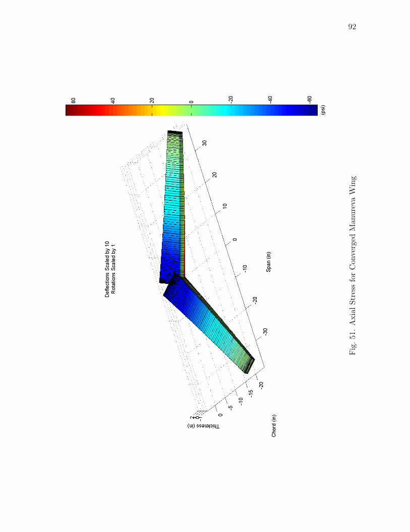
92
Fig
.51
.A
xia
lStr
ess
for
Con
verg
edM
anure
vaW
ing

93
Table VIII. Geometric and Aerodynamic Iteration Results, Twist Adjustments In-
cluded
Iteration 1 Iteration 2 Iteration 3 Iteration 4 Iteration 5
Γ (deg) 0.257242 0.263478 0.270177 0.277146 0.284397
Λ (deg) 30.769966 30.770209 30.770471 30.770743 30.771027
b (in) 74.391546 74.391321 74.391078 74.390824 74.390559
AR 9.997727 9.997667 9.997601 9.997533 9.997462
Twist (deg) 0.248048 0.506790 0.775878 1.055719 1.346732
CL 0.353889 0.360612 0.367754 0.375190 0.382931
CD 0.0066400 0.0067415 0.0068509 0.0069671 0.0070906
The next case includes the adjustments for twist with each iteration, and the
results are shown in Table VIII. As demonstrated by Table VIII, the wing geometric
parameters and aerodynamic coefficients continue to increase with each iteration when
the twist adjustment is included. Only five iterations are shown in Table VIII, but
the trend continues when more iterations are included. Figures 52 and 53 show the
trends of the coefficient of lift and the twist angle for 20 iterations. As the twist
angle increases, the lift also increases which results in an even higher twist angle the
following iteration. The effect is that all of the wing parameters and aerodynamic
coefficients continually increase with each iteration, and no convergence is reached.
The iterative results are different for the two cases evaluated in this research.
For the case where the twist angle is not adjusted with each iteration, the geometric
parameters associated with the wing bending reduced the lift as they increased. The
result was a convergence of the wing parameters and aerodynamic coefficients. The
case where the twist angle is adjusted with each iteration results in a diverging trend

94
0 2 4 6 8 10 12 14 16 18 200.35
0.4
0.45
0.5
0.55
Iteration
CL
Fig. 52. Coefficient of Lift, Twist Adjustment Case
and no convergence occurs. In reality, a wing aeroelastically deflects to a specific twist
angle, as shown in [26]. One potential reason convergence is not reached may be that
the problem is not setup correctly in the interaction tool. An additional stiffness term
due to the aeroelastic effects may need to be included in addition to the strucutal
stiffness matrix which is determined by the structural tool. Because the tool cannot
reach a converged solution for the iterative case which includes the twist adjustment,
the tool will not be practical for detailed aeroelastic analysis. If a torsionally stiff
wing is used for morphing research, the rotational deformations will be small and a
single iteration using the interaction tool may provide more than adequate results.
Overall, the aerodynamic and structural interaction tool works successfully for one
iteration, but future investigation of the convergence case is required in order for the
tool to play a key role in future morphing research.

95
0 2 4 6 8 10 12 14 16 18 200
1
2
3
4
5
6
7
8
Iteration
Tw
ist A
ngle
(de
g)
Fig. 53. Twist Angle, Twist Adjustment Case

96
CHAPTER VI
CONCLUSIONS
This thesis describes the development of a structural analysis tool for a reconfigurable
wing, and it develops an interaction tool which relates the aerodynamic and structural
morphing tools. The structural analysis tool utilizes Space Frame Finite Element
Analysis to model an aircraft wing as an Euler-Bernoulli beam with a solid rectangular
cross section or a box cross section. The structural tool is capable of modeling a wing
with various geometric parameters including wing span, aspect ratio, sweep angle,
dihedral angle, chord length, thickness, and incidence angle. By using variable chord
length, thickness, and incidence along the span, the tool accounts for wing tapering
and twist. Because the tool only models the half-span of the wing, it has the ability
to model asymmetric wing shapes by using the tool once for each half-span.
The aerodynamic and structural interaction tool provides the capability to spec-
ify the morphing wing geometry, run the aerodynamic tool, and run the structural
tool. The loads provided by the aerodynamic tool are used as inputs for the struc-
tural tool to obtain a deflected geometry. The tool makes several valid estimates
regarding the distribution of wing loading, but it does not change the overall nature
of the loads provided by the aerodynamic tool. One version of the interaction tool
includes an iterative method which passes the deflected wing geometry back to the
aerodynamic tool after running the structural tool. It repeats the process of run-
ning the aerodynamic and structural tools for a specified number of iterations. The
tools developed in this research may ultimately be used in conjunction with Machine
Learning tools to learn the structural and aerodynamic impacts of a wide variety of
wing configurations for morphing aircraft.
The following conclusions are made based on the results presented in this thesis:
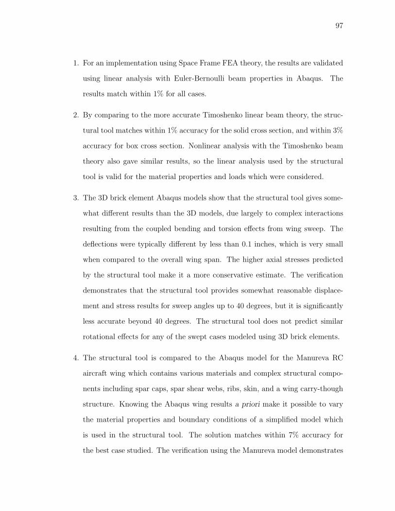
97
1. For an implementation using Space Frame FEA theory, the results are validated
using linear analysis with Euler-Bernoulli beam properties in Abaqus. The
results match within 1% for all cases.
2. By comparing to the more accurate Timoshenko linear beam theory, the struc-
tural tool matches within 1% accuracy for the solid cross section, and within 3%
accuracy for box cross section. Nonlinear analysis with the Timoshenko beam
theory also gave similar results, so the linear analysis used by the structural
tool is valid for the material properties and loads which were considered.
3. The 3D brick element Abaqus models show that the structural tool gives some-
what different results than the 3D models, due largely to complex interactions
resulting from the coupled bending and torsion effects from wing sweep. The
deflections were typically different by less than 0.1 inches, which is very small
when compared to the overall wing span. The higher axial stresses predicted
by the structural tool make it a more conservative estimate. The verification
demonstrates that the structural tool provides somewhat reasonable displace-
ment and stress results for sweep angles up to 40 degrees, but it is significantly
less accurate beyond 40 degrees. The structural tool does not predict similar
rotational effects for any of the swept cases modeled using 3D brick elements.
4. The structural tool is compared to the Abaqus model for the Manureva RC
aircraft wing which contains various materials and complex structural compo-
nents including spar caps, spar shear webs, ribs, skin, and a wing carry-though
structure. Knowing the Abaqus wing results a priori make it possible to vary
the material properties and boundary conditions of a simplified model which
is used in the structural tool. The solution matches within 7% accuracy for
the best case studied. The verification using the Manureva model demonstrates

98
that the structural tool is capable of accurately modeling a complex wing struc-
ture, but requires several good estimates of the structural layout and stiffness
user inputs.
5. The iterative version of the aerodynamic and structural interaction tool showed
that a converged geometry is obtained when the twist angle is not modified dur-
ing each iteration. For the case when twist is modified, the tool showed divergent
behavior in the wing geometric parameters and aerodynamic coefficients. Be-
cause these effects should not occur for the case described, the iterative tool is
not valid when the twist angle is updated each iteration.

99
CHAPTER VII
RECOMMENDATIONS
1. Since twist is a critical aerodynamic parameter, the convergence issue displayed
by the iterative structural interaction tool reduces the utility of the tool for ac-
curate aeroelastic analysis. Further investigation of the aeroelastic convergence
issue must be completed to ensure the tool provides realistic results when the
twist angle is updated with each iteration. One potential solution is to average
each successive rotation angle with the angle calculated by the structural tool
during the first iteration. This method is shown to converge, but the conver-
gence values must be validated using aeroelastic theory or data. An iterative
method is not required to solve the static rotation problem for a cantilevered
swept wing, because an analytical solution to the problem can be obtained.
The ratio between the initial twist angle and the rotation calculated using the
aerodynamic and structural tools during the first iteration may be used with
the analytic solution to determine the final aeroelastically deflected twist angle.
This method is demonstrated for a simplified case in Reference [31].
2. Investigate the aspect ratio limitations inherent in the beam elements used by
the structural tool. 3D brick element wing models with various aspect ratios
ranging from 1 to 9 should be used as comparison cases.
3. Investigate the coupled bending and torsion complex interactions exhibited us-
ing the 3D brick element wing models with sweep. The rotations at the wing
tip determined by the structural tool showed positive angles while the 3D ele-
ment model showed negative angles. A better understanding of the interactions
is required to determine the validity of the structural tool tip rotations when

100
sweep is present.
4. Modify the structural tool to utilize Timoshenko beam theory instead of Euler-
Bernoulli beam theory. As described in [30], Timoshenko beam theory is capable
of modeling beams with a length to thickness ration of 8 to 1, where the thickness
is in the direction of loading, while Euler-Bernoulli beam theory is limited to
a 15 to 1 ratio. A Timoshenko model is fairly similar and would not require
drastic changes to the overall structural tool, but it would allow the ability to
model shorter wings.
5. The structural and aerodynamic interaction tool requires an average CPU time
of 400 seconds for each iteration, and approximately 98% of the computing time
is due to the aerodynamic calculations. An artificial neural network could be
developed to model the aerodynamic tool and provide a more computationally
efficient alternative. Reference [1] demonstrated the ability of a neural net-
work to reduce the computing time of an airfoil panel method by one order of
magnitude.

101
REFERENCES
[1] A. Niksch, “Six Degree of Freedom Morphing Aircraft Dynamical Model with
Aerodynamics,” M.S. Thesis, Texas A&M University, College Station, Texas,
August 2009.
[2] A. Niksch, J. Valasek, T. Strganac, and L. Carlson, “Morphing Aircraft Dynam-
ical Model: Longitudinal Shape Changes,” in Proc. of the AIAA Atmospheric
Flight Mechanics Conference, Honolulu, Hawaii, August 2008, number AIAA-
2008-6567.
[3] A. Lampton, A. Niksch, and J. Valasek, “Reinforcement Learning of Morphing
Airfoils with Aerodynamic and Structural Effects,” Journal of Aerospace Com-
puting, Information, and Communication, Vol. 6, No. 1, January 2009, pp. 30-50.
[4] A. Lampton, A. Niksch, and J. Valasek, “Morphing Airfoil with Reinforcement
Learning of Four Shape Changing Parameters,” in Proc. of the AIAA Guidance,
Navigation, and Control Conference, Honolulu, Hawaii, August 2008, number
AIAA-2008-7282.
[5] A. Lampton, A. Niksch, and J. Valasek, “Reinforcement Learning of a Morphing
Airfoil-Policy and Discrete Learning Analysis,” in Proc. of the AIAA Guidance,
Navigation, and Control Conference, Honolulu, Hawaii, August 2008, number
AIAA-2008-7281.
[6] J. Valasek, M. D. Tandale, and J. Rong, “A Reinforcement Learning - Adaptive
Control Architecture for Morphing,” Journal of Aerospace Computing, Informa-
tion, and Communication, Vol. 2, No. 5, pp. 174-195, April 2005.
102
[7] J. Valasek, J. Doebbler, M. D. Tandale, and A. J. Meade, “Improved Adaptive-
Reinforcement Learning Control for Morphing Unmanned Air Vehicles,” IEEE
Transactions on Systems, Man, and Cybernetics: Part B, Vol. 38, No. 4, August
2008, pp. 1014-1020.
[8] A. Wickenheiser, E. Garcia, and M. Waszak, “Evaluation of Bio-Inspired Mor-
phing Concepts with Regard to Aircraft Dynamics and Performance,” in Proc.
of the SPIE Smart Structures and Materials Conference 2004: Smart Structures
and Integrated Systems, Vol. 5390, 2004, pp. 202-211.
[9] A. Wickenheiser, E. Garcia, and M. Waszak, “Longitudinal Dynamics of a Perch-
ing Aircraft Concept,” in Proc. of the SPIE Smart Structures and Materials
Conference 2005: Smart Structures and Integrated Systems, Vol. 5764, 2005, pp.
192-202.
[10] A. Rodriguez, “Morphing Aircraft Technology Survey,” in Proc. of the 45th
AIAA Aerospace Sciences Meeting and Exhibit, Reno, Nevada, January 2007,
number AIAA-2007-1258.
[11] M. Motamed and J. Yan, “A Reinforcement Learning Approach to Lift Gen-
eration in Flapping MAVs: Simulation Results,” in Proc. of the 2006 IEEE
International Conference on Robotics and Automation, Orlando, Florida, May
2006, pp. 2150-2155.
[12] M. Secanell, A. Suleman, and P. Gamboa, “Design of a Morphing Airfoil Using
Aerodynamic Shape Optimization,” AIAA Journal, Vol. 44, No. 7, pp. 1550-1562,
July 2006.
[13] J. Sater, G. Lesieutre, and C. Martin, “A Smarter Transition for Smart Tech-
nologies,” Aerospace America, June, 2006, pp. 18-21.

103
[14] J. N. Kudva, K. Appa, C. A. Martin, A. P. Jardine, G. Sendeckyj, T. Har-
ris, A. McGowan, and R. Lake, “Design, Fabrication, and Testing of the
DARPA/Wright Lab ‘Smart Wing’ Wind Tunnel Model,” Northrop Grumman,
Wright Laboratory, NASA Langley, 1997.
[15] J. Bowman, B. Sanders, B. Cannon, J. Kudva, S. Joshi, and T. Weisshaar,
“Development of Next Generation Morphing Aircraft Structures,” in Proc. of
the 48th AIAA/ASME/ASCE/AHS/ASC Structures, Structural Dynamics, and
Materials Conference, Honolulu, Hawaii, April 2007, number AIAA-2007-1730.
[16] J. Bae, T. M. Seigler, and D. J. Inman, “Aerodynamic and Static Aeroelastic
Characteristics of a Variable-Span Morphing Wing,” Journal of Aircraft, Vol. 42,
No. 2, pp. 528-534, March-April 2005.
[17] N. A. Ameri, M. H Lowenberg, M. I. Friswell, and E. Livne, “Modelling Contin-
uously Morphing Aircraft for Flight Control,” in Proc. of the AIAA Guidance,
Navigation and Control Conference, Honolulu, Hawaii, August 2008, number
AIAA-2008-6966.
[18] N. Nguyen, “Integrated Flight Dynamic Modeling of Flexible Aircraft with
Inertial Force-Propulsion-Aeroelastic Coupling,” in Proc. of the 46th AIAA
Aerospace Sciences Meeting and Exhibit, Reno, Nevada, January 2008, num-
ber AIAA-2008-194.
[19] J. Manzo, E. Garcia, A. Wickenheiser, and G. C. Horner, “Design of a Shape-
Memory Alloy Actuated Macro-Scale Morphing Aircraft Mechanism,” in Proc.
of the SPIE Smart Structures and Materials Conference 2005: Smart Structures
and Integrated Systems, Vol. 5764, 2005, pp. 232-240.

104
[20] J. Manzo, E. Garcia, A. Wickenheiser, and G. C. Horner, “Adaptive Structural
Systems and Compliant Skin Technology of Morphing Aircraft Structures,” in
Proc. of the SPIE Smart Structures and Materials Conference 2004: Smart Struc-
tures and Integrated Systems, Vol. 5390, 2004, pp. 225-234.
[21] J. N. Kudva and A. Lockyer, “Exploiting Smart Technologies for Military Air-
craft Applications - Perspectives on Development of a Smart Air Vehicle,” in
Proc. of the 40th AIAA/ASCE/AHS/ASC Structures, Structural Dynamics, and
Materials Conference, AIAA/ASME/AHS Adaptive Structures Forum, AIAA
Forum on Non-Deterministic Approaches Conference and Exhibit, St. Louis,
Missouri, April 1999, number AIAA-99-1511.
[22] J. D. Bartley-Cho, D. P. Wang, and J. N. Kudva, “Shape Estimation of Deform-
ing Structures,” in Proc. of the 42nd AIAA/ASME/ASCE/AHS/ASC Struc-
tures, Structural Dynamics, and Materials Conference and Exhibit, Seattle,
Washington, April 2001, number AIAA-2001-1566.
[23] J. E. Hubbard Jr., “Dynamic Shape Control of a Morphing Airfoil Using Spatially
Distributed Transducers,” AIAA Journal of Guidance, Control, and Dynamics,
Vol. 29, No. 3, pp. 612-616, 2006.
[24] D. H. Allen and W. E. Haisler, Introduction to Aerospace Structural Analysis,
New York: John Wiley & Sons, 1985.
[25] W. Weaver Jr. and P. R. Johnston, Finite Elements for Structural Analysis,
Englewood Cliffs, New Jersey: Prentice-Hall, Inc., 1984.
[26] D. H. Hodges and G. A. Pierce, Introduction to Structural Dynamics and Aeroe-
lasticity, New York: Cambridge University Press, 2002.

105
[27] W. Weaver Jr. and J. M. Gere, Matrix Analysis of Framed Structures: 3rd
Edition, New York: Van Nostrand Reinhold, 1990.
[28] P. F. Pai, Highly Flexible Structures: Modeling, Computation, and Experimen-
tation, Reston, Virginia: American Institute for Aeronautics and Astronautics,
Inc., 2007.
[29] A. Campbell, B. Eisenbeis, M. Orr, T. Rudloff, and J. York, Team Manureva:
Structural Wing Design Project Final Report, AERO 405 Course, Professor J.
Whitcomb, College Station, Texas A&M University, 2009.
[30] Abaqus, Inc., Abaqus Analysis User’s Manual, Abaqus Software, Version 6.7,
Providence, Rhode Island: Abaqus, Inc., 2007.
[31] J. Wright and J. Cooper, Introduction to Aircraft Aeroelasticity and Loads,
Chichester, West Sussex, England: John Wiley & Sons Ltd., 2007.

106
APPENDIX A
RESEARCH SCHEDULE

107
23
Fig
8. P
ropose
d R
esea
rch S
ched
ule
Gan
tt C
har
t
Ta
sk N
am
eD
ura
tion
Sta
rtF
inis
h
Lit
era
ture
Se
arc
h7
0 d
ay
sM
on
8/2
5/0
8F
ri 1
1/2
8/0
8
Re
ad
Pa
pe
rs5
0 d
ays
Mo
n 8
/25
/08
Fri 1
0/3
1/0
8
Write
Su
mm
arie
s2
0 d
ays
Mo
n 1
1/3
/08
Fri 1
1/2
8/0
8
2D
FE
A C
od
e1
05
da
ys
Mo
n 9
/8/0
8F
ri 1
/30
/09
FE
A T
he
ory
Re
se
arc
h1
4 d
ays
Mo
n 9
/8/0
8T
hu
9/2
5/0
8
Ma
in P
rog
ram
an
d F
un
ctio
ns S
tiffn
esse
s M
atr
ix, L
oa
ds, S
olv
er,
an
d P
lot D
efle
ctio
n1
4 d
ays
Fri 9
/26
/08
We
d 1
0/1
5/0
8
Fu
nctio
n -
Plo
t D
efle
ctio
n 3
D2
1 d
ays
Th
u 1
0/1
6/0
8T
hu
11
/13
/08
Fu
nctio
n -
Str
ess
14
da
ysF
ri 1
1/1
4/0
8W
ed
12
/3/0
8
Fu
nctio
n -
Plo
t S
tre
ss 3
D4
2 d
ays
Th
u 1
2/4
/08
Fri 1
/30
/09
3D
FE
A C
od
e2
53
da
ys
Mo
n 1
/19
/09
We
d 1
/6/1
0
Sp
ace
Fra
me
Th
eo
ry R
ese
arc
h2
1 d
ays
Mo
n 1
/19
/09
Mo
n 2
/16
/09
Ma
in P
rog
ram
14
da
ysT
ue
2/1
7/0
9F
ri 3
/6/0
9
Fu
nctio
n -
Ge
om
etr
y1
4 d
ays
Mo
n 3
/9/0
9T
hu
3/2
6/0
9
Fu
nctio
n -
Mo
dify
Inp
uts
7 d
ays
Fri 3
/27
/09
Mo
n 4
/6/0
9
Fu
nctio
n -
Ele
me
nt V
alu
es
14
da
ysT
ue
4/7
/09
Fri 4
/24
/09
Fu
nctio
ns -
Stif
fne
ss M
atr
ix a
nd
Co
nstr
ain
ts2
8 d
ays
Mo
n 4
/27
/09
We
d 6
/3/0
9
Fu
nctio
ns -
Dis
trib
ute
d L
oa
ds, P
oin
t L
oa
ds, a
nd
So
lve
r2
1 d
ays
Mo
n 8
/24
/09
Mo
n 9
/21
/09
Fu
nctio
n -
Plo
t D
efle
ctio
n1
4 d
ays
Tu
e 9
/22
/09
Fri 1
0/9
/09
Fu
nctio
n -
P
lot D
efle
ctio
n 3
D2
1 d
ays
Mo
n 1
0/1
2/0
9M
on
11
/9/0
9
Fu
nctio
n -
Str
ess
14
da
ysT
ue
11
/10
/09
Fri 1
1/2
7/0
9
Fu
nctio
n -
Plo
t S
tre
ss 3
D2
8 d
ays
Mo
n 1
1/3
0/0
9W
ed
1/6
/10
Ae
roe
las
tic
ity
10
5 d
ay
sM
on
11
/16
/09
Fri
4/9
/10
Re
se
arc
h A
ero
ela
stic
An
aly
sis
Me
tho
ds
21
da
ysM
on
11
/16
/09
Mo
n 1
2/1
4/0
9
Le
arn
Do
ub
let P
an
el C
od
e1
4 d
ays
Tu
e 1
2/1
5/0
9F
ri 1
/1/1
0
Ma
in P
rog
ram
an
d F
un
ctio
ns C
FD
an
d F
EA
14
da
ysM
on
1/4
/10
Th
u 1
/21
/10
Mo
dify
Ae
rod
yna
mic
Lo
ad
s1
4 d
ays
Fri 1
/22
/10
We
d 2
/10
/10
Ite
rativ
e M
eth
od
14
da
ysT
hu
2/1
1/1
0T
ue
3/2
/10
Re
su
lts
28
da
ysW
ed
3/3
/10
Fri 4
/9/1
0
3D
FE
A C
od
e V
alid
ati
on
an
d L
imit
ati
on
s U
sin
g A
BA
QU
S3
5 d
ay
sM
on
3/8
/10
Fri
4/2
3/1
0
Lin
ea
r B
ea
m T
he
ory
Ca
se
s7
da
ysM
on
3/8
/10
Tu
e 3
/16
/10
No
nlin
ea
r B
ea
m T
he
ory
Ca
se
s1
4 d
ays
We
d 3
/17
/10
Mo
n 4
/5/1
0
3D
Ele
me
nt C
ase
s1
4 d
ays
Tu
e 4
/6/1
0F
ri 4
/23
/10
Th
es
is1
54
da
ys
Mo
n 1
1/1
6/0
9T
hu
6/1
7/1
0
Pro
po
sa
l W
ritin
g2
1 d
ays
Mo
n 1
1/1
6/0
9M
on
12
/14
/09
Pro
po
sa
l E
diti
ng
28
da
ysM
on
1/2
5/1
0W
ed
3/3
/10
Ta
ble
of
Co
nte
nts
an
d S
tru
ctu
re7
da
ysT
hu
3/4
/10
Fri 3
/12
/10
Intr
od
uctio
n7
da
ysM
on
3/1
5/1
0T
ue
3/2
3/1
0
FE
A T
he
ory
7 d
ays
We
d 3
/24
/10
Th
u 4
/1/1
0
FE
A C
od
e7
da
ysF
ri 4
/2/1
0M
on
4/1
2/1
0
FE
A V
alid
atio
n a
nd
Lim
itatio
ns
7 d
ays
Tu
e 4
/13
/10
We
d 4
/21
/10
Ae
roe
lastic
An
aly
sis
7 d
ays
Th
u 4
/22
/10
Fri 4
/30
/10
Ed
itin
g1
4 d
ays
Mo
n 5
/3/1
0T
hu
5/2
0/1
0
De
fen
se
Ch
art
s7
da
ysF
ri 5
/21
/10
Mo
n 5
/31
/10
De
fen
se
Pre
se
nta
tion
1 d
ay
Tu
e 6
/1/1
0T
ue
6/1
/10
Fin
al E
diti
ng
12
da
ysW
ed
6/2
/10
Th
u 6
/17
/10
Au
gS
ep
Oct
No
vD
ec
Ja
nF
eb
Ma
rA
pr
Ma
yJu
nJu
lA
ug
Se
pO
ct
No
vD
ec
Ja
nF
eb
Ma
rA
pr
Ma
yJu
n
Qtr
3, 2
00
8Q
tr 4
, 2
00
8Q
tr 1
, 2
00
9Q
tr 2
, 2
00
9Q
tr 3
, 2
00
9Q
tr 4
, 2
00
9Q
tr 1
, 2
01
0Q
tr 2
, 2
01
0
Fig
.54
.R
esea
rch
Sch
edule
Gan
ttC
har
t

108
VITA
Brian Joseph Eisenbeis was raised in Kansas City, MO. He attended Texas A&M
University, where he received his Bachelor of Science in Aerospace Engineering (2008)
and Master of Science in Aerospace Engineering (2010). He is employed by the Boe-
ing Company in Seattle, WA as part of the Engineering Career Foundation Program.
He may be contacted at the following address:
c/o John Valasek
Texas A&M University
Department of Aerospace Engineering
727D H.R. Bright Building
College Station, TX 77843-3141