U.S. DEPARTMENT OF COMMERCE ENVIRONMENTAL SCIENCE SERVICES ADMINISTRATION

U.S. DEPARTMENT OF THE ARMY CORPS OF ENGINEERS

HYDROMETEOROLOGICAL REPORT NO. 44

Probable Maximum Precipitation Over South Platte River,

Colorado, and Minnesota River, Minnesota

Prepared by

John T. Riedel, Francis K. Schwarz, and Robert L. Weaver

Hydrometeorological Branch, Office of Hydrology, Weather Bureau

Washington, D.C. January 1969

For sale by the Superintendent of Documents, U. S. Government Printing Office Washington, D. C., 20402 Price $1.25.

UDC 551.577.37:551.579.4:551.501.777; 556.121.3 (788) (776) 551.5

-577 ·37

·579

.501

556. .. 121

( 788) (776)

.. 4

.. 777

.. ;

Meteorology Precipitation Excessive falls in short or long periods Hydrometeorology Fluctuations ot: surface water caused by

precipitation Methods of observation and computation Precipitation computation Hydrology Amount and duration of precipitation Maximum amount and duration

Colorado Minnesota

11

Preface

During 1965 there were two outstanding severe floods in the United States that were quite different in the size of area they affected, the character of the rivers in flood, the season of occurrence, the origin of the flood waters, and the remedial measures that might be taken against such floods in the future. But they were similar in that they renewed public interest in the execution of remedial measures against such floods that had been proposed by the Corps of Engineers in previous years. The first of these floods was the great rain and snowmelt floods on the Upper Mississippi and its tributaries in April which was among the most disas­trous ever experienced in these areas.l For example, at Carver on the Minnesota River the previous high stage of 1952 was exceeded by 6 feet. The other flood resulted in great damage along the South Platte River in and near Denver from extremely heavy thunderstorm-type rainfall of about 6 hours duration centered on upstream tributaries to the south of Denver. Both floods were occasioned by intense examples of common meteorological processes in the respective regions and seasons -- snowmelt o~er a broad are~; in spring over the Upper Mississippi and intense short-duration storms to the immediate east of the Rockies during the May - June maximum storm period of that area.

Both of these floods resulted in the Corps of Engineers requesting the Hydrometeorological Branch of the Weather Bureau to prepare probable maxi­mum precipitation estim,ates for basins above prospective dam sites in order to revise and update spillway design floods. In the Upper Mississippi Basin, though the 1965 flood was primarily due to snowmelt, the spillway design flood for any particular dam must of course take into account the possibilities of extreme precipitation localized over the basin immediately above that dam at any time of year, with or without snowmelt depending on the season. The basic method for estimating PMP in the respective regions is the transposition and moisture maximization of storms. Beyond this common base the application and execution of these principles are quite different in the two study areas. The two reports to the Corps of Engineers have been incorporated into this one volume in order to illustrate a vari­ety of methods of estimating probable maximum precipitation.

1 J. L. H. Paulhus, "The March -May 1965 Floods in the Mississippi, Missouri and the Red River of the North Basins," Weather Bureau Technical Report No. 4, August 1967, Washington, D. C.

iii

TABLE OF CONTENTS

PART I

PROBABLE MAXIMUM PRECIPITATION OVER SOUTH PLATTE RIVER BASIN ABOVE CHATFIELD DAM SITE~ COLORADO

CHAPTER I.

CHAPTER II.

CHAPTER III.

CHAPTER IV.

CHAPTER V.

CHAPTER VI.

REFERENCES

INTRODUCTION

METHODS OF ESTIMATING PMP

METEOROLOGY OF MAJOR STORMS

ALL-SEASON PMP

SEASONAL VARIATION

SNOWMELT CRITERIA

PART II

PROBABLE MAXIMUM PRECIPITATION OVER MINNESOTA RIVER~

CHAPTER I.

CHAPTER II.

CHAPTER I II.

INTRODUCTION

PROBABLE MAXIMUM PRECIPITATION ESTIMATES

AND SUMMARY OF REPORT

METEOROLOGY OF MAJOR STORMS IN NO~TH

CENTRAL STATES

CHAPTER IV. ALL-SEASON PROBABLE MAXIMUM PRECIPITATION

CHAPTER V. SEASONAL VARIATION OF PMP

CHAPTER VI. GEOGRAPHIC VARIATION OF PMP IN THE BASIN

CHAPTER VII. TIME AND AREAL DISTRIBUTION

CHAPTER VIII. EXAMPLE OF TIME AND AREAL DISTRIBUTION IN

THE PMP STORM

REFERENCES

ACKNOWLEDGMENTS

v

HINNESOTA

Page

1

3

6

29

49

53

65

67

69

72

75

79

95

99

112

113

114

1-1.

3-1.

3-2. 3-3. 3-4. 3-5. 3-6. 3-7. 3-8.

3-9. 3-10.

3-11. 3-12.

3-13.

3-14. 3-15. 3-16.

3-17a. 3-17b. 3-18. 3-19.

4-1.

4-2.

4-3.

4-4. 4-5. 4-6.

4-7.

FIGURES

Part I

PROBABLE MAXIMUM PRECIPITATION OVER SOUTH PLATTE RIVER BASIN ABOVE CHATFIELD DAM SITE, COLORADO

Areas (sq. mi.) of subbasins of the South Platte drainage above Chatfield Dam site

Monthly mean sea-level pressure (mb.) and 700-mb. heights (10's of feet) and temperatures (°C) - April, May and June Isohyets for four South Platte Basin storms Daily 0500 MST surface maps June 3-4, 1921 Isohyets for indicated 6-hr. periods June 3-4, 1921 Surface maps May 30-31, 1935 Total storm precipitation (in.) June 14-17, 1965 Daily l-in. isohyets to 0700 MST, June 15-18, 1965 Isohyets (in.) for two afternoon storms, one south of Denver June 16, 1965 (upper left) and one east of Colorado Springs June 17, 1965 (lower right) Isohyets (in.) June 15-18, 1965 in southeastern Colorado Average outlines of areas containing thunderstorms on radar during indicated periods June 16-17, 1965 (MST) Average positions of surface front and Low June 14-18, 1965 Daily positions of the sea-level isobar through Denver at 1700 MST June 14-17, 1965 and daily pressure difference between Duluth and E1 Paso Daily positions of the 18,900-ft. 500-mb. height contour at 1700 MST June 14-17, 1965 Composite 850~mb. chart, June 14-18, 1965 Composite 700-mb. chart, June 14-18, 1965 Composite 1000-mb. dew point chart (°F) for 0500 MST June 16 and 17, 1965 "Lifted index" patterns at "Lifted index" patterns at Isohyets (in.) in the June Surface maps for June 6-9,

12-hr. intervals, June 14-16, 12-hr. intervals, June 16-18, 7-8, 1964 Montana storm 1964 (1100 MST)

1965 1965

Generalized all-season enveloping depth-duration curve and supporting data - 439 sq. mi. Generalized all-season enveloping depth-duration curve and supporting data - 1044 sq. mi. Generalized all-season enveloping depth-duration curve and supporting data - 3000 sq. mi. Highest 6-hr. PMP (in.) by subbasin during Pattern-A storm Highest 6-hr. PMP (in.) by subbasin during Pattern-B storm All-season enveloping and sequenced 439-sq. mi. PMP depth-duration relations for Patterns A, B and C All-season enveloping and sequenced 1483-sq. mi. PMP depth-duration relations for Patterns A, B and C

vi

4-8.

4-9a.

4-9b. 4-10.

4-11.

5-1. 5-2.

6-1.

6-2.

6-3.

FIGURES--COntinued

All-season enveloping and sequenced 3018-sq. mi. PMP depth-duration relations for Patterns A, B and C June 16-17, 1965 storm 6-hr. and rearranged cumulative rain block diagrams for 3 storm centers over 439 sq. mi. Accumulated rainfall over 439 sq. mi. Generalized and adjusted 6- and 72-hr. depth-area relations as percent of 1044-sq. mi. depth for,Pattern A Adjusted 6-hr. depth-area relations for Patterns A and B and relations from past storms in percent of 1000-sq. mi. depth

Seasonal variation of maximum 24-hr. precipitation Seasonal variation of physical parameters influencing the adopted seasonal variation of 24-hr. PMP

Adopted maximum free-air wind relations 020° - 180° for South Platte snowmelt computations Adopted relation between free-air and anemometer-level wind with supporting data Adopted 50-ft. anemometer-level winds

Part II

PROBABLE MAXIMUM PRECIPITATION OVER MINNESOTA RIVER, MINNESOTA

1. All-season enveloping PMP for the center of the Minnesota River drainage

2. Minnesota River Basin and storms controlling all-season PMP 3. Seasonal variation for 1-day station maximum precipitation 4a. 1 to 10-day highest precipitation, La Crosse, Wisconsin 4b. 1 to 10-day highest precipitation, Duluth, Minnesota 4c. 1 to 10-day highest precipitation, Huron, South Dakota 4d. 1 to 10-day highest precipitation, Devils Lake, North Dakota 5. Average of 3 highest weekly precipitation values over SW and SE

Minnesota 6. Variation of monthly precipitation over state divisions 7. Seasonal variation from maximized storms 8. Adopted seasonal variation of PMP 9. Variation of precipitation from SE to NW edges of Minnesota

River Basin 10. Geographic variation of PMP in the Minnesota River Basin 11. Isohyets for Minnesota River above Montevideo 12. Isohyets for Minnesota River above Redwood Falls

vii

FIGURES--Continued

13. Isohyets for Minnesota River above New Ulm 14. Isohyets for Minnesota River above Mankato 15. Isohyets for Minnesota River above Carver 16. Isohyets for Chippewa River 17. Isohyets for Cottonwood River 18. Isohyets for Blue Earth River

viii

PART I

PROBABLE MAXIMUM PRECIPITATION OVER SOUTH PLATTE RIVER BASIN ABOVE CHATFIELD DAM SITE, COLORADO

Chapter I

INTRODUCTION

Authorization and assignment

1.01. Authorization for this report is contained in a memorandum from Office of Chief of Engineers, dated December 6, 1965.

1.02. The assignment is to provide 4-day sequenced probable maximum precipitation (PMP) over the South Platte Basin above Chatfield Dam site divided into subbasins 1 through 14 in figure 1-1, with emphasis on the highest 12-hr. period centered over subbasin 9 and an alternate centering over subbasin 6; seasonal variation; and temperature, dew point and wind data for spring snowmelt.

Organization of report

1.03. The report is prefaced by discussion of the problems and methods of estimating PMP in areas like the South Platte (chapter II). Then follows a synopsis of some of the past storms in these areas that influence the estimates (chapter III). Development of the PMP estimates is contained in chapter IV. Seasonal variation is considered in chapter V and snowmelt factors in chapter VI.

39 30

(12)

275

06

.I South Platte below ~ -L Tarryall Mtns.

0 20 MILES

!

jchotfield Dam Site

""' 105

\ Plum Creek

Basin

OCATION MAP DENVER •

Figure 1-1. Areas (sq. mi.) of subbasins of the South Platte drainage above Chatfield Dam site. Numbers in parenthesis designate subbasins.

N

3

Chapter II

METHODS OF ESTIMATING PMP

2-A. Methods in Other Reports

Moisture maximization method

2.01. The method in most general use for estimating the probable max­imum precipitation (PMP) over basins in the United States east of the crest of the Rocky Mountains involves three steps:

a) Maximize observed storms for moisture.

b) Transpose maximized values to the basin. A relocation adjustment is applied, based on moisture, for geographical position and elevation.

c. Envelop transposed maximized values.

These steps are carried out for a range of area sizes and durations that are critical for the basin. Smooth depth-area and depth-duration relations are constructed at the enveloping step. Thus maximized values at one dura­tion and area size have some influence on other durations and area sizes. (This is the method employed in part II.)

2.02. This procedure is based on the following concepts, explained in Hydrometeorological Report Nos. 23 (1) and 33 (2) and other reports. The intensity of precipitation in a storm depends on the available moisture and the mechanisms which produce convergence of the air. All factors favoring precipitation in combination, except moisture, for this purpose are referred to as "storm mechanism.lt If an adequate number of storms can be moisture­maximized and transposed to the basin, it is assumed that one or more of them contains a "storm mechanism" that approaches the probable maximum. The combination with maximum moisture then yields an estimate of the PMP. For this last assumption to be valid the following must prevail:

a) Storms are transposed from a considerable area.

b) Storm records are available for a considerable length of time.

c) A few storms are of outstanding magnitude, as judged by the precipitation in comparison with record values elsewhere and by the resulting floods.

2.03. When these conditions are not fulfilled, other maximization steps that are important for the storm types concerned must be substituted for the moisture maximization or used in combination with it. Thus for

4

basins in the Western United States, where transposition of storms is sharply limited by topography, and where wind is an important factor for orographic precipitation, storms are maximized for both wind and moisture in PMP estimates [Hydromet. Report No. 36 (3)].

Storm combination method

2.04. Another method for basing an estimate of future extreme precip­itation on past rainfall is to combine two or more storms. The storms can be brought together in time closer than actually occurred, or closer to­gether in space, or both. Similarly, bursts in the same storm can be realigned either in space or time. These combinations must of course be meteorologically reasonable and consistent with storm characteristics.

2.05. This combination method was used in forming storm sequences for studies of the flood potential of the Mississippi and Ohio Rivers [Hydromet. Reports Nos. 35 {4) and 38 (5)]. It is commonly used to establish "ante­cedent precipitation" before a 3-day PMP storm derived by the moisture maximization method. It has not been applied generally for 72-hr. PMP estimates in the United States, not because of unsuitability but rather because the moisture maximization or wind maximization methods have gener­ally sufficed.

2-B. Methods in This Report

0 to 12 hours

2.06. The Chatfield PMP to 12 hours is estimated by the moisture maxi­mization and transposition procedure, as the three requirements of paragraph 2.01 are fulfilled:

1. Storms are transposable from a considerable area, consisting of the east slopes of the Rockies and the adjacent plains from the Texas-Oklahoma Panhandle region to Montana.

2. Record is reasonably good for several decades.

3. Some "outstanding" storms have occurred, for example the Cherry Creek storm of May 30-31, 1935 and the June 16-18, 1965 storms. That they occurred near the basin strengthens their value for estimating PMP.

12 to 96 hours

2.07. Moisture-maximization method. For durations beyond 12 hours, the "outstanding storm" criterion does not appear to be fulfilled in the available storms. In the moisture maximization procedure, compensating

5

for this involves considerable reliance on envelopment over duration. Rare occurrences of repeating storms in the Plains States offer some guidance to the amount pf envelopment.

In the moisture maximization method a single isohyetal pattern is used for all durations to distribute the precipitation within the basin for all time increments of the storm. While in a real storm the isohyetal center would not be·expected to remain fixed (unless there are strong orographic controls), assuming that it does yields discharges which approximate those obtained for various critical placements of the rainfall.

2.08. Storm realignment method. A risk not to be neglected for the Chatfield Basin is that the most extreme 6- to 12-hr. precipitation can be preceded or followed by another substantial burst with an intervening brief lapse of precipitation. Once the strong southerly flow and conditions to develop and release instability necessary for the 12-hr. PMP are estab­lished, heavy bursts of rain can be expected within the general region for two or three days. Diurnal heating may combine with stationary terrain effects to encourage repetition at roughly 24-hr. intervals. Therefore the storm realignment method is also used.

Application of methods

2.09. Three patterns of PMP are presented in this report. Patterns A and B are variations of the moisture-maximization method. The Pattern-A rainfall is centered over subbasin 9 (Plum Creek) and that of B over sub­basin 6 of figure 1-1. Pattern C combines moisture maximization and storm realignment. Its rainfall pattern uses a fraction of the highest 6-hr. Pattern-B rainfall, then the highest 6-hr. Pattern-A rainfall, in a manner similar to the rain sequence of the June 16-17, 1965 storm.

6

Chapter III

METEOROLOGY OF MAJOR STORMS

3-A. Climatic Controls on the Extreme Storm

Synoptic pattern

3.01. A necessary condi~ion for extreme rains near PMP caliber in eastern Colorado is the continuing influx ot a rich supply of moisture from the western Gulf of Mexico. Although the normal low-level airflow in April to June is from the Gulf of Mexico {fig. 3-1), it takes a combin­ation of high pressure to northeast and low pressure to southwest to strengthen this flow. If the rain is to be prolonged, a major trough or Low aloft must remain relatively stationary over the Southwestern United States. With this setup, mechanisms for triggering the rain can be effec­tive repeatedly over approximately the same region.

Season of occurrence

3.02. In "Climates of the States" (6) we find the statement "warm moist air from the south moves into Colorado most frequently in the spring. As the air is carried northward and westward to higher elevations, the heaviest and most general rainfalls of the year occur over the eastern portions of the State." Higher average precipitation over eastern Colorado in May and June than in earlier months is apparent by reference to monthly precipita­tion maps in the National Atlas (7). This suggests the possibility of large seasonal differences in extreme storms. But the June flow pattern is nor­mally only a little more favorable for moist inflow than that in earlier months. This is concluded from monthly mean 1000-mb. maps showing flow from the Gulf of Mexico and 700-mb. maps showing a trough to the west of the area {fig. 3-1). Hence the main factor that increases May-June precip­itation potential over earlier months is the increased moisture and instability potential of persistent strong southerly inflow patterns.

3-B. Large Rains Over the Basin

3.03. A twofold purpose is served by study of large rains within the South Platte River drainage above Denver, although the controlling storms are outside the basin. First, they give guidance on distribution of PMP within the basin. Second, they call attention to the important meteoro­logical factors contributing to heavy rain in the basin.

Storm dates

3.04. Table 3-1 contains dates and basin monthly rainfall depths in selected large storms during April, May and June since 1930, obtained from the Decennial Census of United States Climate (8), 1931 to 1960. It was

Sea Level Map 700mb. Map

Figure 3-1. Monthly mean sea-level pressure (mb.) and 700-mb. heights (10 1 s of feet) and temperatures ( 0 ~) - April, May and June.

7

8

surveyed for months having 3 inches or more of precipitation over the Colorado portion of the Platte River drainage. The storms listed, selected from 20 qualifying cases, contain most of the monthly rain in 2 or 3 days. Cases of heavy precipitation over the Platte River drainage in the years 1961 to 1965 are also listed in the table.

Table 3-1

SELECTED HEAVY PRECIPITATION MONTHS OVER THE SOUTH PLATTE BASIN IN COLORADO

Month and Year

April 1933 April 1942 April 1944 June 1949 April 1957 May 1964 June 1965

Precipitation distribution

(1930-1965)

Monthly Basin Precipitation

(in.)

3.40 5.03 3.59 4.71 3.78

Primary Storm Dates

20-22 18-19 9-10 3-4 2-3

29-30 15-17

3.05. Some 2- and 3-day storms that contributed to the high monthly totals shown in table 3-1 were selected to appraise storm precipitation distribution over the South Platte drainage above Denver. Isohyets shown for four of these storms in figure 3-2 demonstrate the large dropoff in precipitation in the more sheltered western portion of the basin. PMP rainfall is judged to drop off in a similar way.

3.06. Similar inferences are drawn from monthly values of maximum 24-hr. rainfall taken from Technical Paper No. 16 (9). Average values for May and June at the longitude of Denver are nearly double those immediately west of the Continental Divide. Less direct support comes from discharge records which do not show any major runoffs from rainfall above Lake George, perhaps largely a result of high infiltration rates.

Typical weather patterns

3.07. Weather maps for large precipitation storms of paragraph 3.05 illustrate that, for extreme rains over the basin, the flow pattern must allow moisture from the Gulf of Mexico to persist over the basin. Common

9

ISOHYETS IN INCHES lSOHYET$ iN lNOit$ AND fENTHS

April 20-22, 1933 April 18-19, 1942 •

l$0HYETS IN INCHES

()

April 9-10, 1944 April 2-3, 195 7

Figure 3-2. Isohyets for four South Platte Basin storms.

10

features of this flow pattern include at lower levels (1) either a counter­clockwise rotation of winds with time as a Low passes eastward to the south of the basin, not unusual, or (2) stagnation of a trough to the west of the basin, a rarer pattern. In either case, there is aloft a Low to the southwest of the basin which reinforces the surface pattern. Stagnation aloft is more common in June, when movements are slowed, than earlier. Its importance is discussed below in connection with the June 1921 and June 1965 storms.

3-C. Extreme Rains Near the Basin

June 3-4, 1921 storm

3.08. The storm of June 3-4, 1921, centered northwest of Pueblo, Colo., was part of a general storm extending from the Texas Panhandle and eastern New Mexico northward through eastern Colorado between the 2d and 6th. Figure 3-3 shows surface charts for the main storm dates. Figure 3-4 shows the isohyets for two successive 6-hr. periods during which the area of intense storm activity shi£ted southeastward from near Penrose to the west of Pueblo. Composite isohyets for these two periods indicate separate bursts overlapping areally.

3.09. The combination of high pressure to the northeast and a weak Low over Arizona caused an influx of moist Gulf of Mexico air into the storm area (above a shallow southward-moving layer of polar air). The importance of a persisting influx of moist air from southeast and its con­trol by broad-scale features can be inferred from daily sea-level pressure differences from the 3d to the 5th between El Paso, Tex. and Duluth, Minn., namely 19, 24 and 20 mbs. There is evidence in recent storms with similar flows that instability can be a concomitant feature.

May 30-31, 1935 Cherry Creek storm

3.10. Several intense rain bursts occurred on May 30-31, 1935 along a line from Cherry Creek, Colo. eastward into northwestern Kansas. This storm is discussed in Hydrometeorological Report No. 13 (10). An intense center occurred over the Cherry Creek Basin, close to the Plum Creek drain­age of the South Platte, on the afternoon of May 30 and another 6 hours later 125 miles to the east-northeast. The brief precipitation was intensified by the approach of a Low moving eastward through Colorado. Figure 3-5 shows this development. For several days prior to the storm there was an influx of moist air from the Gulf of Mexico. The storm motion separated bursts areally far more than in the June 1921 storm (par. 3.08) or the June 1965 storm discussed below.

June 16-17, 1965 storm

3.11. Intense prolonged, widespread thunderstorm activity requires a persistent influx of moisture and extreme instability. The several periods of heavy localized rainfall during June 14-18, 1965 in eastern

Figure 3-3.

Figure 3-4.

JUNE 3 JUNE.

Daily 0500 MST surface maps June 3-4, 1921.

Ca.s.tle Rock~\ \

1500.2100 MST JUNE 3, 1921

c:

Isohyets for indicated 6-hr. periods June 3-4, 1921.

11

-J-<>~/ ·-......, <>p

...-, ·6 I

I f

I

I

/ 1' I 1 , I , I I

-L.J....,._~ _; / \ ,_

\ \

\ I \

\ /-, ~ 298 ............ . \ 1

0600 MST, MAy 30 I

J J

29.9

~

> "-, \. I

~"- I I ','/

I I I

/1 .J __..,..:::..__ 'lqJ

I

I

I ',, t:..:;::...<","

I I

I l;

29.;:.~

" ......,.

I I

\ /-, .... I~ I\

1800 MST, MAY 30 \ 29.s~

'\ \

~"·-"-, I '""'

~ ........ \ I t ') I / --y ._,..

/ ~ ,,, 2pl,, //',

I

ll I

',, 1.[, /'')"-,

\ \

\ I \

\ -, "/ ', .... \

0600 MST, MAY 31 '<9.s I

Figure 3-5. Surface maps May 30-31, 1935. (Sea-level pressure in inches).

•

J

I I I

' ',

~

..... N

Colorado and nearby areas is an outstanding example of pronounced inflow of moist unstable air maintained by a persistent large-scale circulation. Fronts and related synoptic features played a minimal role, as did high­level parameters such as advection of vorticity (11).

3.12. Precipitation maps. Total-storm isohyets (fig. 3-6), taken from the Weekly Weather and Crop Bulletin (12), do not show the large unofficial rainfall amounts. Nor do the outlines of approximate areas of 24-hr. rain to 0700 MST of one inch or more on four successive days

13

of this storm, presented in figure 3-7 as evidence of the persistence of recurring rains in the region. More deta~led maps for specific bursts are shown in figure 3-8. Isohyets for the June 16 Plum Creek storm of approxi­mately 6 hours duration between about 1300 and 1900 MST are shown on the upper left of figure 3-8. The slightly longer period of rain the following afternoon is shown on the right of figure 3-8, centered along an axis to north-northeast from Colorado Springs. A breakdown of this burst into highest 6-hr. rain was made for use in obtaining DDA relations (chap. IV). Figure 3-9 is an isohyetal map for June 15-18 over southeastern Colorado. Most of this rain fell on either the early morning or the evening of the 17th. Because of limited data from bucket surveys and recorders, an approx­imate 6-hr. breakdown of figure 3-9 was based on an estimated percentage of area rainfall.

3.13. Radar rain maps. Three radars (Denver, Colo., Amarillo, Tex. and Goodland, Kans.) provided information on storm progress which is in agreement with the above precipitation maps. Figure 3-10 shows average outlines, during progressive time intervals, of areas within which thun­derstorms or convective showers appeared on one or more of the radars. The average outlines are composites of hourly radar composites (11). Interpo­lated 700-mb. and 500-mb. winds for each time period are aligned approx­imately with the axis of the respective thunderstorm outline.

The outline for the afternoon of the 16th in figure 3-10 encloses the nearly stationary burst over Plum Creek. Cells moved in the same direction as the indicated wind. There followed during the evening a southeastward movement and expansion of the outline (dashed line) within which thunder­storm intensity was fading out. Intensification of thunderstorms took place over the southeastern Colorado portion of the outline during the night. Weakening there during the morning of the 17th was followed by intensification again that evening, and clockwise rotation of the outline, as shown. Meanwhile, a new outline appears to the northwest on the after­noon of the 17th, representing the burst shown on the right of figure 3-8.

3.14. Persisting inflow. During this storm both surface and upper-air flow patterns were remarkably stable. This is evident in the following discussion of these patterns.

14

Figure 3-6. Total storm precipitation (in.), June 14-17, 1965.

I----- I I --

1

JUNE 15 JUNE 16

I

I

I I COL.9!A_££-

JUNE 17 JUNE 18

Figure 3-7. Daily l-in. isohyets to 0700 MST, June 15-18, 1965.

I I I I \

Denver \

1 11 I / I

June 16, 1965 1 ', I

'l I ,.../ I

,1 I . ) //

,..; I , ---1 1 1/ '"1

I I I

I /

(

') I )

( ) \ )

I I

I 1

/'-1 I 1 11

II I / I I I

I I j / I (---

1 I ) 1 I r\ I ~ ( I I .._; \ I _) (\ I I ,/"" \~

-/ / ( I/ ) I I

( I I 'I I 1 1

I I

I \ I \

Colorado ,Springs.,

I I I

I 6 ( \ 1

10

STATUTE MILES

June 17, 1965

20 I

15

Figure 3-8. Isohyets (in.) for two afternoon storms, one south of Denver, June 16, 1965 (upper left) and one east of Colorado Springs, June 17, 1965 (lower right).

---~

I I

--- --r:l--1"' location Map tJ "' SCALE 1:500,000

0! QV.O

~~ o,:z cs;J ul

I 2

I

J I

I 2 I I

Figure 3-9. Isohyets (in.) June 15-18, 1965 in southeastern Colorado. (Most of the rain fell in the early morning or the late evening of the 17th.)

1-' 0"

WIND ---700mb. -----500mb.

I I

AMA~ILLO l_, '

17

Figure 3-10. Ave1age outlines of areas containing thunderstorms on radar during indicated periods June 16-17, 1965 (MST). Winds for each period at 700 mb. and 500 mb. are areally interpolated.

18

1. Surface

3.15. The synoptic sequence is pictured schematically in figure 3-11. With high pressure over the Northern Plains, a weak Low developed in southern Nevada as a wave on a front on the i4th. Both moved across Utah on the 15th and into western Colorado that night. The Low then moved northward and filled in southern Wyoming on the morning of the 16th. During the following important rain periods of the 16th and 17th, the weak north­south front remained stationary near the Continental Divide and west of the rain areas.

A continuous low-level flow from the southeast prevailed to the east of the Continental Divide during the entire period. Its persistence is shown in figure 3-12 by tracing on successive days the 1700 MST sea-level isobar through Denver upstream toward the Gulf. Large daily sea-level pressure differences between Duluth, Minn. and El Paso, Tex. exceeded those in the June 1921 storm (par. 3.09). They were 23, 27, 32 and 24mb. for the 14th through 17th, respectively.

2. Aloft

3.16. Evidence of persistence in the upper-air pattern is shown in figure 3-13 by the nearly stationary positions of the 18,900-ft. contour plotted from daily 1700 MST 500-mb. maps. It is shown also by height contours on June 14-18 composite charts for the 850-mb. level (fig. 3-14) and the 700-mb. level (fig. 3-15), averages of twice-a-day upper-air obser­vations. The line of zero departure from normal 700-mb. heights in figure 3-15 (from the Gulf through eastern Colorado) parallels the tongue of moisture at 850-mb., shown by dew point lines on figure 3-14, a feature which correlates with precipitation.

3.17. Moisture criteria. All extreme rainstorms over sizable areas require a continuing strong influx of moisture. This was realized in the June 1965 storm, as shown by both surface and upper-air analyses of moisture.

Composite 850-mb. and 700-mb. moisture fields for June 14-18, 1965 are shown by dew point lines in figures 3-14 and 3-15, respectively. There is agreement on the two charts in the positions of the moist tongue extending along the high plains from the Gulf of Mexico, although the 700-mb. moist tongue is downwind of the simultaneous 850-mb. moist tongue, as is typical during periods of extreme thunderstorms.

Figure 3-16 shows 0500 MST June 16-17 composite 1000-mb. dew points obtained by adjusting observed dew points moist adiabatically to 1000 mb. In this chart of representative moisture near the surface, the axis of the moist tongue agrees with positions at 850 and 700mb., figures 3-14 and 3-15, respectively.

I I

,__ I I -------.} L tl

I I 1005 lC'

j L __ WYo=--L/

,' 142300-lSJJOOM L / __.)(- - - ----r ,

--, / L 997 ,/

/ L x{ 1902 I 9980xl

I I I / 1 GRA_ND

I 0~ / 1 JUNCTION -- n"!,o,. -- ,., ... ;,..; rl'tYt _ I

,s,.,_29· ..---~f:l_j L - - JlRIZ 1 -~

I · o

I II ff I 0

I I 0

~ r

0 PUEBLO

_£0LO ..

NEWMEX1 I I

I I I

I -- r---r---__

--1

I I

__j

I l I

I I I

_j

Figure 3-11. Average positions of surface front and Low June 14-18, 1965.

19

20

"-- /

I

Figure 3-12. Daily positions of the sea-level isobar through Denver at 1700 MST June 14-17, 1965 and daily pressure difference between Duluth and El Paso.

Figure 3-13. Daily positions of the 18,900-ft. 500-mb. height contour at 1700 MST June 14-17, 1965.

f'"' 4500 I -..,

J I

I I

/ I

"" 4500 I I I

' I I I \

' \.

I I

I

' ' ' \ \ t--_ I /". \ ~,>, \ ~ \ '-- __ ,--,

\ \ I I I I I \ \

'.... \ \ '"'- I )

\ \ ', \ I '\ I I 1 \ l ' \ ' '

' l

4600 4700

---

____- Helght contour {ft.)

4700

I

/ f

I

I I I I \

1 (

I I I

/

Figure 3-14. Composite 850-mb. chart, June 14-18, 1965.

Figure 3-15.

/ I I

I \

I

I I l I

(

/ I

--,,..,......,, "

Composite 700-mb. chart, June 14-18, 1965.

1 \

' ' ' I 'J

21

22

60

I -- -

53 e

52 ·--' 60

' \ 65 \ \ \ \

\

67 41

' - .,/

67 •

72 •

' '7J ' . \ \

I

/68 •

I I I I

I

70 •

\ \

\ \ ~2

70 \

e63

60

63 •

60

67 41 65

......

' - -66 ---•

68 •

67 •

67 •

13 70 • 73

• 73

76 • / • /

....... ,...., 74 / • /

/ I

Figure 3-16. Composite 1000mb. dew point chart (°F) for 0500 MST June 16 and 17, 1965.

23

3.18. Instability. In seeking causes of the heavy rain bursts of June 16 and 17, the role of instability must be considered. Intense thunderstorms re~uire high moisture in the low levels. With minor changes in temperature aloft, the influx of warm moist air at low levels appears to be the important destabilizing influence. The combination becomes appar­ent in negative values of "lifted index" (13). The values are obtained in this report by lifting the lowest 1500-ft. layer to the level of free convection dry adiabatically and then moist adiabatically to the 500-mb. level where the lifted layer temperature is compared to the environmental temperature. This temperature difference is a good indicator of the buoyancy forces that will be available to permit local extreme precipita­tion. The 1500-ft. layer adequately measures moisture influx in this storm. The negative lifted index values are larger in absolute magnitude than values of the Showalter Index (14). Both represent unstable conditions.

Analyses of the lifted index for successive 12-hr. periods June 14-18, 1965 (figs. 3-17a, b) show areas of highly unstable air aligned toward eastern Colorado from the south Texas coast. Their correspondence to the areas of high moisture in figures 3-14 through 3-16 demonstrates in a general way the importance of a combination of high moisture and high in­stability for extreme release of convective rainfall.

3.19. The degree of instability in this storm was increased by inso­lational heating, especially near the mountains. This is evident by the progressive buildups over foothill areas of convective shower intensity during midday to a climax during the afternoon. Both the June 16 Plum Creek area burst and that to the east the following day (fig. 3-8) began shortly after noon, as indicated by both mass curves and hourly radar patterns. Reports of tornadoes, lightning and hail damage from the 14th through the 17th are largely confined to afternoon and evening hours except in areas to the east at lower elevations. An example is the severe thunderstorm that moved down Big Thompson Canyon to the Loveland area at midafternoon of the 14th.

3.20. Conclusions. Causes of the bursts of rainfall in the June 1965 storm are not evident on synoptic charts by fronts, squall lines or moving Lows. Rather, the evidence points to the moisture influx at lower levels (15) and instability enhanced by terrain lifting and daytime heating as important causes. The pronounced persistence of inflow of moist unstable air over a fixed area supports the potential for even a more critical placement and timing of rainfall bursts than occurred in this particular storm.

3-D. More Distant Storms

3.21. An example of heavy orographic rainfall on the eastern slopes of the Continental Divide is the June 7-8, 1964 Montana storm. Its weather patterns provide a clue to rainfall a similar storm might produce in the

24

MST June 14 1700

1700 MST June 15

Figure 3-17a. ~~Lifted index " patterns a

MST June 15 0500

t 12-hr. 14-16, 1965. intervals June

25

Del Rio

1700 MST June 16

Figure 3-17b. "Lifted index11 patterns at 12-hr. interva1s)June 16-18, 1965.

26

South Platte Basin. In chapter IV, rainfall data from this storm are transposed to areas of the basin where such a storm would provide signifi­cant rainfall; most areas in the basin are lee areas to its upslope flow.

Isohyets of storm rainfall (about 30 hours duration) and lines of percent of mean annual precipitation are shown in figure 3-18 for the Montana slopes and lee areas north of 47°N. They emphasize the large addi­tion of rainfall on slopes facing east and northeast as a strong flow of moist air moved northward into Montana from the Gulf of Mexico~ then westward directly up these slopes on the 7th and 8th, as shown on daily surface maps (fig. 3-19}. This upslope flow was prolonged by presence aloft of a persistent Low over the Northwest. The large rainfall amounts on foothills (fig. 3-18) point to release of instability as a factor in the general rainfall over the area. Its combination with lifting on slopes directly exposed to inflow account for the extreme rainfall. Transposition of this storm to a less well-exposed basin involves various adjustments.

Figure 3-18. Isohyets (in.) in the June 7-8, 1964 Montana storm. (Dashed lines are percents of mean annual precipitation.)

27

28

June 6 June 7

June 8 June 9

Figure 3-19. Surface maps for June 6-9, 1964 (1100 MST).

29

Chapter IV

ALL-SEASON PMP

4.01. Development of PMP values is along the following lines: (a) A basic 6-hr. PMP value for 439 square miles (area of the Plum Creek drainage) is derived by maximization and transposition of storm data. (b) DDA rela­tions to extend this value to PMP for longer durations and larger areas are derived from a combination of additional storm data and judgment. (c) PMP magnitudes are developed from these generalized relations, modified to con­form to the South Platte Basin for orographic effects and for differences between storms in the basin and east of the basin. (d) Final PMP values are presented as subbasin averages in a sequence form for the three storm centerings described in paragraphs 4.09 and 4.17. DDA relations therefrom are then compared with the generalized relations and those from storms.

It is convenient to discuss (a) the 6-hr. PMP values, (b) the depth­duration and (c) the depth-area relations separately even though they are intimately related and are not obtained independently.

4-A. 6-Hour 439-Square Mile PMP

4.02. Maximization of pertinent observed storm rainfall by table 4-1~ transposition to the Plum Creek Basin, and envelopment lead to a 6-hr. 439-sq. mi. PMP estimate of 12.0 inches. The adopted value is shown in figure 4-1, along with supporting data. The Cherry Creek storm of May 1935 and the less well-documented southeastern Colorado storm of June 17, 1965 jointly support this level of PMP for 6 hours. The latter is adjusted from 5000 ft. to 7700 ft. elevation. The Cherry Creek value is not reduced for elevation since it was-observed at an elevation only slightly less than that of the Plum Creek drainage.

4.03. In order to insure geographical consistency of the adopted level with values elsewhere, a pattern was drawn of 6-hr. 500-sq. mi. PMP for the region surrounding the basin which took into account the topography in a general manner. This confirmed that the 12 inches in six hours is consistent with a regional pattern of PMP.

4-B. Generalized DDA Relations

4.04. Rainfall DDA relations from Storm Rainfall (16) and other sources were investigated,in record storms near the South Platte drainage and along east slopes of the Rocky Mountains. The more important of these storms are listed in table 4-1.

Date

5/30-31/35 6/16/65 6/17/65 6/17/65 6/2-6/21 5/29-31/94 4/14-16/21 10/19-24/08 4/29/14-5/2/14 6/17-21/21 9/27/23-10/1/23 9/20-23/41 6/23-28/54

Table 4-1

J~OR STORMS PROCESSED IN DEVELOPING PROBABLE MAXIMUM PRECIPITATION VALUES

Place

Cherry Creek, Colo. Plum Creek, Colo. Eastonville, Colo. Holly, Colo. Penrose, Colo. Ward District, Colo. Fry's Ranch, Colo. Meeker, Okla. Nara Visa, New Mex. Springbrook, Mont. Savageton, Wyo. McCo1leum Ranch, New Mex. Pandale, Tex.

Assignment No.* Transposed Moisture Adjustment

(Storm Date)

MR 3-28A 1.28 - 1.34 - 1. - 1.34

sw 1-23 1.48 MR 6-14 1.81 MR 4-19 1.91 sw 1-11 1.71 sw 1-16 1.41 MR 4-21 1.41 MR 4-23 1.28 GM 5-19 1.11 sw 3-22 1.16

Elevation Adjustment to 7700 •

1.00 0.96 0.94 0.78 0.88 0.96 1.02 0.60 0.86 0.70 0.84 o. 0.68

*Ref. 16, Corps of Engineers, U. S. Army, "Storm Rainfall in the United States, 11

Washington, 1945-.

w 0

31

Three sizes of area were selected for analysis of DDA relations, 439, 1044 and 3000 square miles. These areas approximate, respectively, the Plum Creek drainage, the area below the Tarryall Mountain Divide excluding the Plum Creek drainage (1483-439), and the total basin. Storm rainfall values for these areal sizes were moisture-maximized, then transposed to the basin by adjusting for geographical variation of maximum moisture and for barrier elevation, as discussed in paragraph 4.18. The depth-duration and depth-area relations developed from these storm data are referred to as "generalized" relations to distinguish from the basin "adjusted" rela­tions plotted from final PMP values. Differences are explained in paragraph 4.28.

Generalized depth-duration relations

4.05. The depth-duration envelopes for these three ar~a sizes are shown in figures 4-1 through 4-3. That for 439 square miles is drawn to closely envelop the Cherry Creek and June 1965 storms (chapter III) for 6 and 12 hours duration. These storms are most useful in defining the short-duration (6-hr. and 12-hr.) PMP for the 439-sq. mi. Plum Creek Basin and the eastern half of the total basin, of greatest interest for evaluation of runoff.

4.06. The envelope beyond 12 hours is obtained by liberal envelopment of the data, since it is clear that storms in this region have not approach­ed their potential beyond 12 hours as closely as they have for shorter durations, as discussed in paragraph 2.07. Liberal envelopment is supported also by the observed repetition of severe storms within a limited area (e.g., June 14-18, 1965) and the reasoning of paragraph 2.08 which is based on such repetition, The Pandale, Tex. storm (plotted on figs. 4-1 through 4-3), though not of a type transposable to the basin without modification, also illustrates the possibility of large rain amounts beyond one day.

Generalized depth-area relations

4.07. The three depth-duration curves just described (figs. 4-1 through 4-3) provide data from which generalized depth-area curves may be drawn for any duration. For illustration, figure 4-10 shows the Pattern A generalized depth-area curves for 6 and 72 hours (--) based on these depth­duration curves.

4-c. Patterns A and B Subbasin PMP

4.08. The 6-hr. 439-sq. mi. PMP and the generalized DDA relations pro­vide the framework of PMP values which are altered by certain basin effects.

Storm centering

4.09. Two basic storm centerings of PMP isohyetal patterns are em­ployed in this report, in accordance with the letter of assignment.

"

NOTE: Data and curve adjusted to 7700 feet

@

e @

"* ~ 12~ / 0 0 • 0 0 ~ .. * A I 0 ..

-!)-A

* :; CODE DATE @ 6.-¢- A • 5/30-31/35 0 • ; w X 6/16/65 0

0 6/17/65 AX-t -o-E9 • 6/17/65 @ .. A 0 6/2-6/21

@ ~ A 5/29-31/94 .(1- ~ .. 4/14-16/21 e ... 10/19-24/08 ~ t 4/29/14-5/2/14 .. 6/17-21/21 t:. e 9/27/23-10/1/23

~ 9/20-23/41 @ 6/23-28/54

oL I I I I I I 48

DURATION (HRS.)

e

"* A

PLACE Cherry Creek, Colo. Plum Creek, Colo. Eastonville, Colo.

Holly, Colo. Penrose, Colo Word District, Colo. Fry"s Ranch, Colo. Meeker, Okla . Nora Visa, N.M. Springbrook, Mont. Savogeton, Wyo.

Me Colleum Ranch, N.M. Pandale, Tex.

ASSIGN. NO. MR 3-28A

sw 1-23 MR 6-14 MR 4.19 sw 1-11 sw 1.16 MR 4-21 MR 4-23 GM 5-19 sw 3-22

96

Figure 4-1. Generalized all-season enveloping depth-duration curve and supp(>rting data -439 sq. mi. Plotted data have no seasonal adjustment.

w N

CODE DATE PlACE ASSIGN. NO.

• 5/30-31/35 Cherry Creek, Colo. MR 3-28A

X 6/16/65 Plum Creek, Colo.

0 6/17/65 Eostonville, Colo.

• 6/17/65 Holly, Colo.

0 6/2-6/21 Penrose, Colo. sw 1-23

6. 5/29-31/94 Word District, Colo. MR 6-14

A 4/14-16/21 Fry's Ranch, Colo. MR 4-19

... 10/19-24/08 Meeker, Oklo. SW 1.11

t 4/29/14-5/2/14 Nora Visa, N.M. sw 1-16

6/17-21/21 Springbrook, Mont. MR 4-21

e 9/27/23.10/1/23 Savogeton, Wyo. MR 4-23

ll?J 9/20-23/41 Me Colleum Ranch, N.M. GM 5.19

® 6/23-28/54 Pondole, Tex.

~ ®

Figure 4-2. Generalized all-season enveloping depth-duration curve and supporting data -1044 sq. mi. Plotted data have no seasonal adjustment. w

w

CODE DATE PlACE ASSIGN. NO. 0 5/30-31/35 Cherry Creek, Colo. MR 3-28A X 6/16/65 Plum Creek, Colo.

c 6/17/65 Eastonville, Colo.

II 6/17/65 Holly, Colo.

0 6/2-6/21 Penrose, Colo sw 1-23

t::. 5/29-31/94 Word District, Colo. MR 6-14 <1. 4/14-16/21 Fry's Ranch, Colo. MR 4.19

• 10/19-24/08 Meeker, Oklo. sw 1-11

-¢- 4/29/14-5/2/14 Nora Visa, N.M. sw 1-16

* 6/17-21/21 Springbrook, Mont. MR 4-21

e 9/27/23.10/1/23 Savageton, Wyo. MR 4-23

181 9/20-23/41 Me Co Ileum Ranch, N.M. GM 5-19

@ 6/23-28/54 Pandole, Tex. SW 3-22

<.{) w J: v 12 z I _,.,..-

@ @

181 @ • t::. @

~ ¥ i t::.e

* i A 0 @H} e 0 181

• "/). 0 0 181 ~ .0

181

IL~ ~ e ~ ~

NOTE: Doto and curve adjusted to 9800 feet

or I I I I I I I I I I I j 48 60 72 84 96

DURATION (HRS.)

Figure 4-3. Generalized all-season enveloping depth-duration curve and supporting data -3000 sq. mi. Plotted data have no seasonal adjustment.

w

""'

~ Plum Creek

Basin

Figure 4-4. Highest 6-hr. PMP (in.) by subbasin during Pattern~ storm.

Figure 4-5. Highest 6-hr. PMP (in.) by subbasin during Pattern-B storm.

35

IJ) w J: 12 v ~

b.

b.

Adiusted Envelopes

(see par. 4.25)

----~

ok==±:: I I I I I I I I I I I I I I I '" "' "' 48 60 72 84 96

DURATION (HRS.)

Figure 4-6. All-season enveloping and sequenced 439-sq. mi. PMP depth-duration relations for Patterns A, B and C. The generalized envelope is shown for comparis:on.

!,;.) 0\

., ILl

:t: 12 u ~

o•·-

/ .... ..-

........ ....

48 DURATION (HRS.)

96

Figure 4-7. All-season enveloping and sequenced 1483-sq. mi. PMP depth-duration relations for Patterns A, B and c. w .....

V> ..... 512 ~

ol==-t----t- I I I I I I I I I I I I I I ,.,. ..,, ~~- 48 60 72 84 96

DURATION {HRS.)

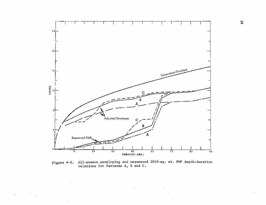
Figure 4-8. All-season enveloping and sequenced 3018-sq. mi. PMP depth-duration relations for Patterns A, B and C.

VJ 00

39

Pattern A is centered over subbasin 9 and places the 439-sq. mi. PMP within the Plum Creek Basin, on the edge of the total basin. Pattern B is con­structed to give the 439-sq. mi. Pattern-A volume reduced for barrier by 10 percent (par. 4.18), with the center over subbasin 6.

PMP subbasin averages

4.10. 6 hours. The 6-hr. 439-sq. mi. value from paragraph 4.02, posi­tioned in paragraph 4.09, was extended to the rest of the basin with barrier reduction (par. 4.18), relying primarily on paragraph 4.07 and the 6-hr. depths in figures 4-1 through 4-3 for depth-area relations. There result maps of subbasin average values shown in figure 4-4 for Pattern A and fig­ure 4-5 for Pattern B.

4.11. 12 to 96 hours. The adopted enveloping values for longer dura­tions are obtained by extending the 6-hr. amounts on a percentage basis with depth-duration curves. A spectrum of depth-duration relations for area sizes up to 3000 square miles could be employed to obtain PMP for any duration and area size from the 6-hr. pattern. It is characteristic of storms that incremental depths drop off less steeply with duration as area (i.e., distance from the storm center) increases. This characteristic is closely approximated in this report by use of the 439-sq. mi. depth-duration relation of figure 4-1 (in percent of highest 6-hr.) over roughly 439 square miles and the 1044-sq. mi. relation of figure 4-2 over the remainder of the basin. The procedure is summarized below.

Pattern

A B

Sequencing PMP

Depth-duration relation

439-sq. mi. (from fig. 4-1) 1044-sq. mi. (from fig. 4-2)

subbasins 8, 9 subbasins 3a, 4, 5, 6

rest of area rest of area

4.12. The rule employed in sequencing PMP for both Patterns A and B was to place the daily values in the following sequence: 3d highest, 2d highest, highest and 4th highest. This is shown in the sequenced PMP of the A and B Patterns in tables 4-2 and 4-3 and in figures 4-6 through 4-8.

4.13. Recognition of the diurnal effect leads to alternating large and small 12-hr. values. Daily amounts other than for highest day are split into 12-hr. amounts of approximately 20 percent and 80 percent of daily amounts. This explains the step appearance of portions of the sequenced mass curves of figures 4-6 through 4-8.

4~D. Pattern C Subbasin PMP

12-hr. PMP

4.14. In Pattern C the highest 12-hr. PMP is identical to that of Pattern A.

40

30-hr. PMP

4.15. The 30-hr. Pattern-C PMP over the eastern half of the basin is increased approximately 2 inches over the Pattern-A 30-hr. PMP and sequenced as two bursts separated both in time and space with a 6-hr. rainless inter­val in between. This 2-in. net increase is after barrier reduction to that portion of the precipitation that is shifted westward.

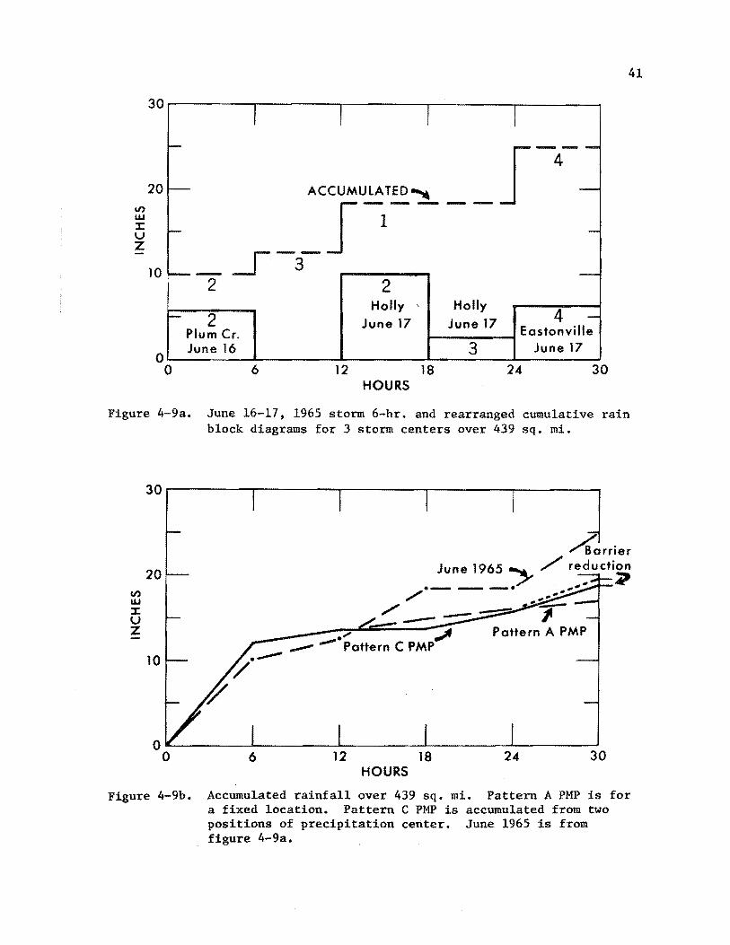
4.16. Basis. The 30-hr. Pattern-C PMP value is based on experience in the June 16-17, 1965 storm. Figure 4-9a shows the succession of bursts over 439 square miles in this storm in the time sequence in which they oc­curred but regardless of their location. The Holly center is in extreme southeastern Colorado (fig. 3-9 inset). Also shown is an accumulation of these observed amounts rearranged, with 25 inches in 30 hours.

This accumulated June 1965 439-sq. mi. rainfall graph of figure 4-9a is drawn as a line in figure 4-9b, along with the Pattern-A adjusted PMP envelope of figure 4~6 for comparison. The adopted Pattern-C 30-hr. enve­lope of two storm centers in figure 4-9b is a compromise between the June 1965 rainfall curve based on three relatively widely separated storm centers and the Pattern-A envelope based on a single center. This Pattern-C envelope, taking into account a 10 percent barrier reduction for the last 12 hours of the curve, is 2 inches higher than the Pattern-A envelope at 30 hours. The 18- to 30-hr. increment is 5.3 inches.

PMP sequencing and centering for 96-hr. storm

4.17. The first part of the sequenced Pattern-C storm, 0- to 42-hr., is approximately that of the sequenced Pattern B for all zones, with the same centering over subbasin 6. Next, the 5.3-in. 18- to 30-hr. increment of 439-sq. mi. Pattern-C PMP (par. 4.16 and fig. 4-9b) is placed in the Pattern-C sequence at 42 to 54 hours and centered as in the Pattern B in subbasin 6 (fig. 4-6); extension to larger areas (figs. 4-7 and 4-8) is as discussed in paragraph 4.11. A 6-hr. period of no rain follows. Then 12-hr. PMP for all zones is placed at 60 to 72 hours as in Pattern A cen­tered over the Plum Creek Basin. It is followed by Pattern A sequenced PMP 72 to 96 hours. The sequenced PMP values are listed in table 4-4 and shown as cumulative values for 3 sizes of area in figures 4-6 through 4-8.

Second highest 6-hr. amount in Pattern C (figs. 4-6 through 4-8) is placed 18 hours in advance of highest 6-hr. amount. This is the shortest possible interval between bursts whose timing is controlled by diurnal effects. A 6-hr. period of no rain is considered typical between such rain bursts on successive days.

en w J: v z

30 r----,-,--.-, -----,-,----,1----,

-

20 f--

10 r------2

ACCUMULATED~ J_3_I_l __ 2

Holly June 17

6 12 18 HOURS

__ I-4-~

Holly June 17

24

-

-

30

41

Figure 4-9a. June 16-17, 1965 storm 6-hr. and rearranged cumulative rain block diagrams for 3 storm centers over 439 sq. mi.

en w J: v z

30r-------~--------~--------.-------~--------~

20

10

OL---------~--------~--------~--------~------~ 0 6 12 18 24 30

HOURS

Figure 4-9b. Accumulated rainfall over 439 sq. mi. Pattern A PMP is for a fixed location. Pattern C PMP is accumulated from two positions of precipitation center. June 1965 is from figure 4-9a.

~ N

Table 4-2

PMP FOR PATTERN A

Area Sq. Mi. Basin 0 12 24 36 48 54 60 66 72 84 96 Hours -324 9 .5 1.9 .1 2.5 1.1 1.3 13.0 1.8 .4 1.6 Inches

115 8 .4 1.4 .5 1.8 .8 .9 9.2 1.3 .3 1.1 Total

439 Ave. .5 1.8 .6 2.3 1.0 1.2 12.0 1.7 .4 1.5 23.0

82 6 .4 1.5 .5 1.9 .8 1.2 8.4 1.5 .3 1.3 222 5 .4 1.3 .5 1.8 .8 1.1 8.0 1.4 .3 1.2 240 7a .3 1.1 .4 1.4 .7 1.0 6.2 1.1 .2 1.0

39 4 .3 1.6 .5 2.0 .9 1.3 6.8 1.2 .3 1.0 101 3a .3 1.6 .5 2.0 .9 1.3 6.8 1.2 .3 1.0

54 3b .2 .8 .3 1.1 .4 .7 4.2 .8 .2 .7 146 2 .2 .9 .3 1.2 .6 .8 4.8 .9 .2 .7 160 1 .3 1.1 .3 1.5 .7 .9 6.0 1.1 .2 .9

1483 Ave. .3 1.4 .5 1.8 .8 1.1 8.1 1.3 .3 1.1 16.7

239 7b .1 .5 .3 .9 .4 .5 3.0 .5 .1 .5

1722 Ave. .3 1.3 .5 1.7 .7 1.0 7.4 1.2 .3 1.0 15.4

333 10 .1 .3 .3 1.0 .5 .7 1.6 .2 .1 .3 290 14 .1 .3 .1 .5 .2 .3 2.0 .3 .1 .3 262 11 0 .1 0 .8 .4 .5 .8 .1 0 .1 136 13 0 .1 0 .2 .1 .1 .8 .1 0 .1 275 12 0 .1 .1 .6 .3 .4 .6 .1 0 .1

3018 Ave. .2 .8 .3 1.3 .6 .8 4.8 .8 .2 .7 10.5

Area Sq. Mi. Basin 0 12 24 36

324 9 .4 1.4 .5 115 8 .4 1.5 .5 82 6 .5 1.9 .6

222 5 .4 1.5 .5 39 4 .4 1.9 .5

101 3a .4 1.8 .5

444 Ave. .4 1.7 • 5~

54 3b .4 1.5 .5 240 7a .5 1.9 .6 146 2 .4 1.5 .5 160 1 .4 1.5 .5

1483 Ave. .3 1.6 .6

239 7b .3 1.4 .4

1722 Ave. .3 1.6 .6

333 10 .2 .7 .3 290 14 .2 .9 .2 262 11 .1 .3 .2 136 13 .1 .3 .1 275 12 0 .2 .2

3018 Ave. .2 1.1 .4

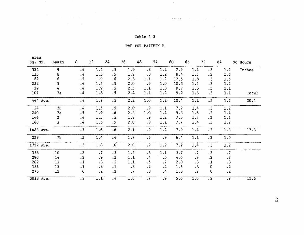
Table 4-3

PMP FOR PATTERN B

48 54 60

1.9 .8 1.2 7.9 1.9 .8 1.2 8.4 2.3 1.1 1.2 12.5 2.0 .9 1.0 10.3 2.5 1.1 1.3 9.7 2.4 1.1 1.2 9.2

2.2 1.0 1.2 10.4

2.0 .9 1.1 7.7 2.3 1.0 1.4 9.3 1.9 .9 1.2 7.5 2.0 .9 1.1 7.7

2.1 .9 1.2 7.9

1.7 .6 .9 6.4

2.0 .9 1.2 7.7

1.5 .6 1.1 3.7 1.1 .4 .5 4.6 1.1 .5 .7 2.0

.3 .2 .2 1.5

.7 .3 .4 1.3

1.6 .7 .9 5.6

66 72 84

1.4 .3 1.5 .3 1.8 .3 1.4 .3 1.3 .3 1.3 .3

1.2 .3

1.4 .3 1.6 .3 1.3 .3 1.4 .3

1.4 :3

1.1 .2

1.4 .3

.7 .2

.8 .2

.3 .1

.3 0

.2 0

1.0 .2

1.2 1.3 1.5 1.2 1.1 1.1

1.2

1.2 1.4 1.1 1.2

1.3

1.0

1.2

.7

.7

.3

.2

.2

.9

96 Hours

Inches

Total

20.1

17.6

12.6

.$::­w

~ ~

Table 4-4

PMP FOR PATTERN C

Area Sq. Mi. Basin 0 12 24 36 42 48 54 60 66 72 84 96 Hours

-324 9 .3 1.4 .5 .8 3.0 1.9 0 13.0 1.8 .4 1.6 Inches 115 8 .3 1.5 .5 .8 3.2 2.0 0 9.2 1.3 • .3 1.1

439 Ave. 12.0 1.7 .4 1.5

82 6 .5 1.9 .6 1.0 4.0 2.5 0 8.4 1.5 • .3 1.3 222 5 .4 1.5 .5 .8 3.3 2.1 0 8.0 1.4 • .3 1.2

39 4 .3 1.4 .5 .8 3.1 1.9 0 6.2 1.2 .2 1.0 101 3a .3 1.4 .5 .7 2.9 1.8 0 6.8 1.2 • .3 1.0

444 Ave. .4 1.5 .5 .8 3.3 2.0 0

54 3b .3 1.4 .5 .8 2.9 1.8 0 6.8 1.2 • .3 1.0 240 7a .4 1.8 .5 .9 3.5 2.2 0 4.2 .8 .2 .6 146 2 .3 1.4 .4 .7 2.9 1.8 0 4.8 .9 .2 .7 160 1 .2 1.4 .5 .8 3.0 1.8 0 6.0 1.1 .2 .9 Total

1483 Ave. .3 1.5 .5 .8 3.2 1.9 0 8.1 1.3 .3 .9 18.8

239 7b .3 1.2 .4 .6 2.4 1.7 0 3.0 .5 .1 .5

1722 Ave. .3 1.5 .5 .8 3.1 1.9 0 7.4 1.2 .3 .9 17.9

333 10 .2 .6 .3 .6 2.2 1.4 0 1.6 .3 .1 .2 290 14 .2 .9 .2 .4 1.8 1.1 0 2.0 .4 .1 .3 262 11 .1 .3 .2 .4 1.5 .9 0 .8 .1 0 .1 136 13 .1 .3 .1 .1 .6 .4 0 .8 .1 0 .1 275 12 0 .2 .2 .2 1.0 .6 0 .6 .1 0 .1

3018 Ave. .2 1.0 .4 .6 2.4 1.5 0 4.8 .8 .2 .6 12.5

45

4-E. Topographic Adjustments

Barrier adjustments

4.18. The topography within the basin necessitates adjustment of maxi­mized storm data and enveloping values. A south to southeast wind direction is assumed during the PMP storm. A 7700-ft. barrier then applies to the 439-sq. mi. Plum Creek drainage. Over the remainder of the basin (average barrier 9800 ft.) an additional 10 percent barrier reduction was applied, representing the loss of moisture in a column between 7700 and 9800 feet.

This 10 percent barrier reduction is incorporated in the 1044-sq. mi. and 3000-sq. mi. depth-duration relations (figs. 4-2 and 4-3) for the areas to which they pertain.

Orographic rain additions

4.19. While the emphasis in this report is on convective rain poten­tial, that for orographic rain over higher slopes is considered for a portion of the 4-day period when convective rain is not large.

4.20. A measure of extreme orographic precipitation over the higher slopes of the basin is obtained by transposing an extreme storm from outside the basin. The selected prototype is the June 1964 30-hr. Montana storm on the east slope of the Rocky Mountains (fig. 3-18). Computations of 30-hr. orographic rain in the storm show an average depth of 6.8 inches.

4.21. This Montana storm computation is transposed to the western slopes of the South Platte Basin where a 130° wind direction is assumed. Adjustments to storm moisture for change in average elevation and in lati­tude from Montana to the South Platte are found to cancel each other. Adjustment is made for difference in the average slope at the two locations. Average slope rain is distributed over slopes in subbasins 7a, 7b, 10, 11, and 12 as a percentage of that on the average slope according to moisture to be lifted and actual lift involved relative to average slope values of moisture and lift. Volumes are totaled by subbasin and divided by area to obtain average subbasin depths. Orographic rain is placed in the sequence during the 30 hours from the 24th to the 54th hour, so as to precede the period when convective centers are most significant. Its variation is based on the sequential variation of 24- to 54-hr. PMP in Patterns A and B.

4.22. Amounts on slopes of the Tarryall Mountains, not as satisfac­torily evaluated because of the various orientations of slopes, are accounted for by increasing 24- to 54-hr. rain amounts of Patterns A and B by 10 per­cent in subbasins 1 and 2 and 30 percent in subbasins 3a and 4. In Pattern C these subbasins have large amounts of convective rain during this 30-hr. interval and no orographic addition is made.

46

Adjusted PMP values

4.23. Values of subbasin and total basin all-season PMP for 6- or 12-hr. sequenced intervals shown in tables 4-2 through 4-4 for Patterns A, B and C, respectively, include topographic adjustments outlined above.

4-F. Adjusted DDA Relations

4.24. The subbasin PMP values of tables 4-2 through 4-4 can be assem­bled into "adjusted11 DDA relations for comparison with the generalized relations.

Adjusted depth-duration relations

4.25. Adjusted depth-duration envelopes for three area sizes (439, 1483 and 3018 sq. mi.), representing the Plum Creek drainage, the area below the Tarryall Mountain Divide and the total basin, are shown in figures 4-6 through 4-8, respectively, for Patterns A, B and C. They are drawn to cumulative PMP values from tables 4-2 through 4-4 (PMP Patterns A, B and C, respectively), after ranking incremental durational amounts in descending order of magnitude. The generalized envelopes from figures 4-1 through 4-3 are replotted on figures 4-6 through 4-8, respectively, for comparison. (The 1482-sq. mi. generalized envelope of fig. 4-7 is summed from the 439-and 1044-sq. mi. curves of figs. 4-1 and 4-2.)

4.26. Comparison with generalized relations. For 439 square miles (fig. 4-6), the adjusted depth-duration envelope for Pattern A agrees with the generalized envelope. The Pattern-B adjusted envelope is roughly 10 percent lower because of barrier reduction. With increase in area size to 1483 square miles (fig. 4-7) and 3018 square miles (fig. 4-8), the ad­justed envelopes drop increasingly below the generalized envelope, especially in Pattern A, for the reasons given in paragraph 4.28.

The exceedance of the adjusted Pattern-C envelope over the adjusted Pattern-A envelope for the 439- and 1483-sq. mi. areas (figs. 4-6 and 4-7) is in line with use of two centerings during the Pattern-C storm (par. 4.16).

Adjusted depth-area relations

4.27. The 6- and 72-hr. adjusted depth-area curves are shown by dashed lines (---) in figure 4-10. They are obtained by plotting vs. area the 6- and 72-hr. subbasin PMP depths, tabulated as in table 4-2. Also shown by solid lines (--) are the corresponding generalized relations.

4.28. Comparison with generalized relations. The generalized and ad­justed relations of figures 4-6 through 4-8 and figure 4-10 differ increas­ingly with area increase for several reasons. The generalized curves

</) w .... w

"' <

3000

2000

::J 800 a </)

500

-- GENERALIZED

==:..:_ADJUSTED

PERCENT

47

Figure 4-10. Generalized and adjusted 6- and 72-hr. depth-area relations as percent of 1044-sq. mi. depth for Pattern A.

4000

3000

</) 2000 w _.

~ w

"' < ::J a </)

800

Figure 4-11. Adjusted 6-hr. depth-area relations for Patterns A and B and relations from past storms in percent of 1000-sq. mi. depth.

48

prescribe PMP volumes centered symmetrically over the eastern portion of the basin in such a way that all the rain fits in the basin. As area in­creases, this assumption becomes more and more unrealistic. Likewise, the inaccessibility of the western portion of the basin to widespread convective storms, compared to areas farther east, requires that the depths in the adjusted depth-area curves of figure 4-10 drop off much more rapidly at larger basin sizes than in the generalized curves. Depths in Pattern B, centered farther west than Pattern A, drop off less rapidly with increasing area. as shown for 6 hours in figure 4-11.

4.29. Comparison with storm relations. Figure 4-11 shows selected storm depth-area curves for 6 hours, plotted as a percent of the 1000-sq. mi. depth. The final Pattern-A curve approximates the curves for the May 1935 Cherry Creek storm and the June 16-17, 1965 storms. The adjusted Pattern-B curve lies close to that of the June 1921 Penrose storm. Both curves drop off more steeply with basin sizes above 2000 sq. mi. than do curves of .ob­served storms (typical of bordering areas east of the South Platte Basin) because of relative inaccessibility of western subbasins to widespread convective storms.

DDA comparisons with Hydrometeorological Report No. 33 values

4.30. PMP values read from HMR 33 (2) for 439 square miles over Plum Creek at June 15 are plotted in figure 4-6 for comparison with the adjusted Pattern-A envelope. That they are higher than the adjusted envelope for short durations is largely because of a different seasonal adjustment of the controlling May 31 Cherry Creek value, in Report No. 33 by seasonal varia­tion of moisture and in the envelope of figure 4-6 by the flatter seasonal curve developed in chapter V.

49

Chapter V

SEASONAL VARIATION

5.01. Seasonal variation of PMP for the South Platte Basin is examined in the light of seasonal variation of storm rainfall, temperature gradients, available moisture, and other data. This leads to adoption of an increase from March through June 15 and no change during the following month.

Rainfall as a clue

5.02. Observed maximum rains of record in the Rocky Mountain foothills and the Plains of eastern Colorado provide the basic data for evaluating seasonal variation. The inclusion of additional stations over a larger area helps to compare seasonal variation in the eastern Colorado area with that in surrounding regions.

5.03. Summaries of maximum monthly rains of record over climatic regions (8) for months March through July, considered jointly, show an in­crease in monthly precipitation magnitude from March to June and little change thereafter.

5.04. A similar relation in monthly maximum 24-hr. precipitation (ex­pressed in percent of mid-June) is found for the average of 12 eastern Colorado Plains stations (curve A of fig. 5-l) and for the average of se­lected stations farther east (curve B). An earlier peak in May noted in curve C, an average for nine Colorado foothill stations, is believed due in part to orographic increase in early spring precipitation at the latter stations. Such an increase is more typical of the general storm discussed in chapter 3-b than of the localized intense precipitation of storms dis­cussed in chapter 3-c, the prototype storm for PMP.

Other clues

5.05. As mentioned in chapter II, both moisture and storm mechanism influence PMP. One measure of storm mechanism is temperature contrast, which represents potential energy subject to transformation into kinetic energy in storms. As a qualitative indicator of temperature contrast, the maximum 1000- to 700-mb. thickness gradient within 300 miles of Denver on monthly normal maps is plotted in percent of mid-June in figure 5-2 (curve A). Curve B is an indicator of seasonal variation of moisture. It shows, in percent of June values, seasonal variation of precipitable water (represented by monthly maximum 1000-mb. dew point averaged for Denver, Pueblo and Amarillo and an assumed moist adiabatic lapse rate). Curve C is the product of these two parameters.

50

Features of seasonal variation

5.06. The adopted seasonal variation of PMP, based on data described in paragraphs 5.04 and 5.05, is shown in figures 5-l and S-2. For the period prior to June 15 the adopted seasonal variation of PMP has the following features:

1. It fairly closely parallels the mean of curves A and B of figure 5-l and allows more springtime rainfall than indicated by Hydrometeorologi­cal Report No. 33.

2. It shows more increase April to June than the product of precipi­table water and thickness gradient (fig. S-2).

5.07. From June 15 through July 15, PMP is assumed constant as a compromise of contrary indications from the seasonal variation of the various parameters shown in figures 5-l and S-2.

5.08. The various tables and figures in this report pertaining to PMP values for earlier dates are linearly interpolated as a percentage of June 15 PMP by use of table 5-l.

Table 5-1

SEASONAL PERCENTS OF JUNE 15 PMP

~ Percent of June 15

April 15 71 May 1 81 May 15 90 June 1 96 ~une 15 100 July 15 100

51

120

100 w z :::::> .... 1.1..

0 80 1-

z w u ~ 1.1.1 a..

60

40~------~------~------~--------L-----~ MAR APRIL MAY JUNE JULY AUG

Figure 5-l. Seasonal variation of maximum 24-hr. precipitation. Observed values are compared with adopted and rlliR #33 relations. Inset map shows data sources.

52

w z :::> ..... 1.1..

0 1-z w v 0.: w 0..

A "MAXIMUM 1000- 700mb THICKNESS GRADIENT WITHIN 300 MilES Of DENVER ON NORMAL MAPS

B:: AVERAGE PRECIPITABLE WATER BASED ON MAXIMUM 1000-mb 180 DEW POINTS AT DENVER, PUEBLOANDAMARILLOAND A MOIST

160

140

120

100

80

60

ADIABATIC lAPSE RATE.

PRODUCT OF A AND B

.......... ····;:;..·~ .·· ,. .· /

c......_ •• •• "" ........ .I' ... · /

ADOPTED~/ /

/

/

...... ------

40~------~------~------~~------~------~ MAR APRIL MAY JUNE JULY AUG

Figure 5-2. Seasonal variation of physical parameters influencing the adopted seasonal variation of 24-hr. PMP.

53

Chapter VI

SNOWMELT CRITERIA

6.01. A rational approach to snowmelt computations requires estimates of snowpack and various basin parameters such as albedo and forest cover. Also required, both during and prior to the PMP precipitation, are reasona­bly extreme sequences of temperatures, dew points and winds compatible with other adopted basin PMP criteria. Snowmelt 'winds, temperatures and dew points are provided in tables 6-2 through 6-4 for three days of PMP and in tables 6-5 through 6-7 for three days prior to the 3-day PMP sequence. Values are presented for April 15, May 15, and June 15 PMP placement. A breakdown by 1000-ft. increments of elevation is provided in the tables. As noted on tables 6-6 and 6-7, a mean daily temperature higher than 62°F. is not to be used over snow cover.

Snowmelt winds

6.02. Seven years of upper wind data restricted in direction from 20° through east to 180° were surveyed for Denver for the months April through July. In addition a survey was made of maximum 24-hr. surface winds at Denver and Pueblo, Colo. These data give information on magnitude of free­air winds.

6.03. Adopted free-air winds. Adopted free-air maximum 1-day winds from these data are shown in figure 6-1, with a single wind envelope for April and May and a lower one for June. This seasonal variation is sug­gested by the data.

6.04. Winds reduced to anemometer level. The winds appropriate for snowmelt computations are the free-air winds reduced to an anemometer level of 50 feet. A comprehensive study (3) of ratios of anemometer wind at Blue Canyon, Calif. (with a 50-ft. well-exposed anemometer) to oakland, Calif. free-air wind at the same elevation suggests a ratio of 0.75. A similar comparison of 850-mb. winds averaged for North Platte, Nebr. and Dodge City, Kans., with Denver's 20-ft. anemometer winds is made in figure 6-2. Also shown is the same curve adjusted to a 50-ft. anemometer level by the 6th power law (17). It supports a ratio less than that indicated by the Blue Canyon study. A recent study based on windflow over an Alaskan glacier gives a ratio of 0.60, considered appropriate to wind over unforested ter­rain of average exposure (18). A 0.65 ratio was adopted for the South Platte drainage. The resulting 50-ft. anemometer-level winds are shown in figure 6-3.

6.05. Durational variation. During three days of PMP, durational variation of wind is derived from a consideration of winds during the June 1965 storm period and during other selected prototype storms with an

54

easterly wind component. No consistent dependance of durational variation on elevation was found; a single variation was therefore adopted. This is shown as percent of maximum day in table 6-1.

1 2 3

Table 6-1

DURATIONAL VARIATION OF WIND

Percent of Highest Day

100 80 67-1/2

For three days prior to PMP, 67-1/2 percent is used. This makes allow­ance for the fact that a directional restriction on wind is not necessary for this antecedent period.

Winds at 50-ft. anemometer level during three days of PMP are shown in tables 6-2 through 6-4 and for three prior days in tables 6-5 through 6-7 at mid-month April through June, respectively. They were obtained by apply­ing the percents of highest day to values in figure 6-3.

Snowmelt temperatures

6.06. During precipitation. Temperatures and dew points during pre­cipitation are defined by the maximum 12-hr. persisting dew point in combi­nation with the durational variation of high dew points at Denver. This variation amounts to a 1.7°F. decrease the first day and an additional 1.3°F. decrease the second day of rain prior to the 24-hr. PMP.

6.07. Antecedent to precipitation. Temperature departures from the normal were determined at Leadville, Colo. and at stations at lower eleva­tions in or near the basin for the first, second and third days prior to the beginning of storm periods between mid-April and mid-June. The plot of these data has no seasonal variation. The adopted excess above normal is 3°, 6°, and 9° on the first, second and third prior days, respectively, any time during the spring snowmelt season. Such departures are considered the extreme prior to the PMP storm.

Snowmelt dew points

6.08. Dew points and temperatures are assumed equivalent during PMP (par. 6.06). For the three days prior to PMP the adopted dew points are equal to temperatures (par. 6.07) minus appropriate temperature-dew point differences based on representative differences prior to storms.

55

6.09. Based on evidence from observed lapse rates, the adopted eleva­tion variation of temperature and dew point during PMP is the moist adia­batic lapse rate (tables 6-2 through 6-4). The variation for the three days prior to the precipitation is 4°F. per 1000 ft. (tables 6-5 through 6-7).

Seasonal variation of adopted criteria

6.10. Seasonal variation of the adopted temperature and dew point during PMP at midmonth, April through June, is tied directly to the seasonal variation of the maximum persisting dew point. This variation is shown in tables 6-2 through 6-4.

6.11. The seasonal variation of temperature prior to PMP is taken from Denver's month-to-month variation of mean temperature. Seasonal Varia­tion of dew point parallels that of temperature since the adopted tempera­ture dew-point differences are the same April through June.

Evaluation of adopted criteria

6.12. Adopted temperatures, including elevation variations, were com­pared with mean and maximum temperatures of record. These comparisons demonstrated the reasonableness of the adopted criteria in the light of the storm prototype.

56

Table 6-2

TEMPERATURE, DEW POINT AND WIND DURING 24-HOUR APRIL PMP AND PRIOR TWO DAYS OF RAIN

Elevation Date Temp. and Dew Point *Wind (ft.) (oF.) (mph)

5000 April 13 45.6 26 April 14 46.9 39 April 15 48.6 31

6000 April 13 42.8 26 April 14 44.1 39 April 15 45.8 31

7000 April 13 40.0 27 April 14 41.3 40 April 15 43.0 32

8000 April 13 37.1 28 April 14 38.4 41 April 15 40.1 32

9000 April 13 34.2 29 April 14 35.5 43 April 15 37.2 34

10,000 April 13 31.2 30 April 14 32.5 43 April 15 34.2 35

11,000 April 13 28.1 30 April 14 29.4 45 April 15 31.1 36

12,000 April 13 24.8 32 April 14 26.1 48 April 15 27.8 38

13,000 April 13 21.5 34 April 14 22.8 49 April 15 24.5 40

14,000 April 13 18.2 35 April 14 19.5 52 April 15 21.2 41

15,000 April 13 14.8 36 April 14 16.1 54 April 15 17.8 43

*Appropriate to 50-ft. well-exposed anemometer.

57

Table 6-3

TEMPERATURE, DEW POINT AND WIND DURING 24-HOUR MAY PMP AND PRIOR TWO DAYS OF RAIN

Elevation Date Temp. and Dew Point *Wind (ft.) (oF.) (mph)

5000 May 13 51.4 26 May 14 52.7 39 May 15 54.4 31

6000 May 13 48.8 26 May 14 50.1 39 May 15 51.8 31

7000 May 13 46.2 27 May 14 47.5 40 May 15 49.2 32

8000 May 13 43.5 28 May 14 44.8 41 May 15 46.5 32

9000 May 13 40.8 29 May 14 42.1 43 May 15 43.8 34

10,000 May 13 38.0 30 May 14 39.3 43 May 15 41.0 35

11,000 May 13 35.2 30 May 14 36.5 45 May 15 38.2 36

12,000 May 13 30.2 32 May 14 33.5 48 May 15 35.2 38

13,000 May 13 29.3 34 MllyJ4 30.6 49 May 15 40

14,000 May 13 26.3 35 May 14 27.6 52 May 15 29.3 41

15,000 May 13 23.2 36 May 14 24.5 54 May 15 26.2 43

*Appropriate to 50-ft. well-exposed anemometer.

58

Table 6-4

TEMPERATURE, DEW POINT ANI> WIND DURING 24·HOUR JUNE PMP AND PRIOR TWO DAYS OF RAIN

Elevation Date Temp. and Dew Point *Wind (ft.) (oF.) (mph)

5000 June 13 57.2 21 June 14 58.2 31 June 15 60.2 24

6000 June 13 54.8 22 June 14 55.8 31 June 15 57.8 25

7000 June 13 52.4 22 June 14 53.4 32 June 15 55.4 26

8000 June 13 50.0 23 June 14 51.0 34 June 15 53.0 27

9000 June 13 47.6 24 June 14 48.6 36 June 15 50.6 28

10,000 June 13 45.0 24 June 14 46.0 36 June 15 48.0 28

11,000 June 13 42.4 25 June 14 43.4 37 June 15 45.4 30

12,000 June 13 39.8 26 June 14 40.8 38 June 15 42.8 31

13,000 June 13 37.2 27 June 14 38.2 40 June 15 40.2 32

14,000 June 13 34.4 28 June 14 35.4 41 June 15 37.4 32

15,000 June 13 31.6 30 June 14 32.6 44 June 15 34.6 35

*Appropriate to 50-ft. well-exposed anemometer.

59

Table 6-5

TEMPERATURE, DEW POINT AND WIND PRIOR TO APRIL 13-15 RAIN

Elevation Date Temp. Dew Point *Wind (ft.) ("'F.) (oF.) (mph)

5000 April 10 58.1 41.6 26 April 11 55.1 42.6 26 April 12 52.1 43.6 26

6000 April 10 54.1 37.6 26 April 11 51.1 38.6 26 April 12 48.1 39.6 26

7000 April 10 50.1 33.6 27 April 11 47.1 34.6 27 April 12 44.1 35.6 27

8000 April 10 46.1 29.6 28 April 11 43.1 30.6 28 April 12 40.1 31.6 28

9000 April 10 42.1 25.6 29 April 11 39.1 26.6 29 April 12 36.1 27.6 29

10,000 April 10 38.1 21.6 30 April 11 35.1 22.6 30 April 12 32.1 23.6 30

11,000 April 10 34.1 17.6 30 April 11 31.1 18.6 30 April 12 28.1 19.6 30

12,000 April 10 30.1 13.6 32 April 11 27.1 14.6 32 April 12 24.1 15.6 32

13,000 April 10 26.1 9.6 34 April 11 23.1 10.6 34 April 12 20.1 11.6 34

14,000 April 10 22.1 5.6 35 April 11 19.1 6.6 35 April 12 16.1 7.6 35

15,000 April 10 18.1 1.6 36 April 11 15.1 2.6 36 April 12 12.1 3.6 36

*Appropriate to 50-ft. well-exposed anemometer.

60

Table 6·6

TEMPERATURE, DEW POINT AND WIND PRIOR TO MAY 13-15 RAIN

Elevation Date Temp. Dew Point *Wind (ft.) (oF.) (oF.) (mph)

Use 62°F. 5000 May 10 66.5 as maximum 47.4 26

May 11 63.5 mean daily 48.4 26 May 12 60.5 temperature 49.4 26

6000 May 10 62.5 over snow 43.4 26 May 11 59.5 44.4 26 May 12 56.5 45.4 26

7000 May 10 58.5 39.4 27 Mayll 55.5 40.4 27 May 12 52.5 41.4 27

8000 May 10 54.5 35.4 28 May 11 51.5 36.4 28 May 12 48.5 37.4 28

9000 May 10 50.5 31.4 29 May 11 47.5 32.4 29 May 12 44.5 33.4 29

10,000 May 10 46.5 27.4 30 May 11 43.5 28.4 30 May 12 40.5 29.4 30

11,000 May 10 42.5 23.4 30 May 11 39.5 24.4 30 May 12 36.5 25.4 30

12,000 May 10 38.5 19.4 32 May 11 35.5 20.4 32 May 12 32.5 21.4 32

13,000 May 10 34.5 15.4 34 May 11 31.5 16.4 34 May 12 28.5 17.4 34

14,000 May 10 30.5 11.4 35 May 11 27.5 12.4 35 May 12 24.5 13.4 35

15,000 May 10 26.5 7.4 36 May 11 23.5 8.4 36 May 12 20.5 9.4 36

*Appropriate to 50-ft. well-exposed anemometer.

61

Table 6-7

TEMPERATURE, DEW POINT AND WIND PRIOR TO JUNE 13-15 RAIN

Elevation Date Temp. Dew Point *Wind (ft.) (oF.) (oF.} (mph)

5000 June 10 77.5 53.2 21 June 11 74.5 54.2 21 June 12 71.5 55.2 21

6000 June 10 73.5 Use 62°F. 49.2 22 June 11 70.5 as maximum 50.2 22 June 12 67.5 mean daily 51.2 22

7000 June 10 69.5 temperature 45 •2 22 June 11 66.5 over snow 46 •2 22 June 12 63.5 47.2 22

8000 June 10 65.5 41.2 23 June 11 62.5 42.2 23 June 12 59.5 43.2 23

9000 June 10 61.5 37.2 24 June 11 58.5 38.2 24 June 12 55.5 39.2 24

10,000 June 10 57.5 33.2 24 June 11 54.5 34.2 24 June 12 51.5 35.2 24

11,000 June 10 53.5 29.2 25 June 11 50.5 30.2 25 June 12 47.5 31.2 25

12,000 June 10 49.5 25.2 26 June 11 46.5 26.2 26 June 12 43.5 27.2 26

13,000 June 10 45.5 21.2 27 June 11 42.5 22.2 27 June 12 39.5 23.2 27

14,000 June 10 41.5 17.2 28 June 11 38.5 18.2 28 June 12 35.5 19.2 28

15,000 June 10 37.5 13.2 30 June 11 34.5 14.2 30 June 12 31.5 15.2 30

*Appropriate to 50-ft. well-exposed anemometer.

62

20 ---- E9- £:..-- 6

I

---------·- L 500 18

£:.. Ap•il Do"'" SO· Y••• wiod \ I 0 Moy Denver 50- Yeor wind Single obs.

I E9 June Denver 50· Year wind (1957- 63)

I • April moximum daily wind I 16 at Denver 11950- 64]

~ Some May 0 0 Some June

A April Pueblo mox doily (1950- 64) I 14

* Moy Pueblo mox doily (1950 64] I • June Pueblo mox doily (1950- 64)

I .... (All odjusted by sixth power

A =ADOPTED APRil, MAY ...... "' I FREE AIR WIND (DAilY) 0 low from 22' to 72') .....

J: 0 ell ~ ~ 0 12 • June 1965 storm mox single obs. I ~ - ~ w ..... wind over Denver B ADOPTED JUNE J: ::c I ~ FREE AIR WIND (DAILY) w I ::c

10 I -·- E9 0 -- 700 3

I I J 8 I

I I

0£:.. - - - - - - - ------, E9- 2

6 I

d::> me:.. -··-* __ _L_ ---------- 850

4 20 40 60 80 100 120

MPH

Figure 6-1. Adopted maximum free-air wind relations 020° - 180° for South Platte snowmelt computations.

60,-------.--------r-------r-------,--------r-------,-------,--------.--,

50

z 40 Q.

.§.. t.f) 0 z j ~ 30 1-IJJ

~ 0 ~ IJJ z < 20

10

/ /

/ Blue Canyon (50') /

\ / y

Adopted Relation

/

/

/~ y

, '\ /.laskan Glacier

/

,./ '/" /~

//~

• •

0~------~------~-------L------~--------L-------~-------L ______ _L __ ~

0 10 20 30 40 50 60 70 ao FREE-AIR WINDS (mph)

Figure 6-2. Adopted relation between free-air and anemometer-level wind with supporting data. 0\ w

60

:X: 0.. 40 ~

20

4 6 B 10 12

HEIGHT !1000's ft.)

Figure 6-3. Adopted 50-ft. anemometer-level winds.

14 16

0"­.p.

REFERENCES

l. U. S. Weather Bureau, "Generalized Estimates of Maximum Possible Precipitation over the United States East of the 105th Meridian for Areas of 10, 200, and 500 Square Miles," Hydrometeorological Report No. 23, Washington, 1947.

65

2. U. S. Weather Bureau, "Seasonal Variation of Probable Maximum Precipitation East of the 105th Meridian for Areas from 10 to 1000 Square Miles and Durations of 6, 12, 24 and 48 Hours," Hydrometeoro­logical Report No. 33, Washington, 1956.

3. U. S. Weather Bureau, "Interim Report - Probable Maximum Precipitation in California," Hydrometeorological Report No. 36, Washington, 1961.

4. U. S. Weather Bureau, '~eteorology of Hypothetical Flood Sequences in the Mississippi River Basin," Hydrometeorological Report No. 35, Washington, 1959.

5. U. S. Weather Bureau, '~eteorology of Flood-Producing Storms in the Ohio River Basin," Hydrometeorological Report No. 38, Washington, 1961.

6. U. S. Weather Bureau, Climatography of the United States No. 60-5, "Climates of the States -Colorado," 1959.

7. Environmental Data Service, "Climatic Maps of the United States­Normal Total Precipitation," ESSA, U. S. Department of C0011nerce, 1965.

8. U. S. Weather Bureau, '~ecennial Census of the United States Climate, Monthly Averages for State Climatic Divisions 1931-1960," Clima­tography of the United States No. 85, 1963.

9. U. S. Weather Bureau, ·~aximum 24-Hour Precipitation in the United States," Technical Paper No. 16, 1952.

10. U. S. Weather Bureau, "A Report on the MaxiDilm Possible Precipitation over Cherry Creek, Colorado," Hydrometeorological Report No. 13, 1940.

11. U. S. Weather Bureau, "Heavy Rains in Colorado June 16 and 17, 1965," Central Region Technical Memo No. 4, 1966.

12. U. S. Weather Bureau, "Weekly Weather and Crop Bulletin," vol. 52, No. 25, June 1965, p. 1.

13. U. s. Weather Bureau, "Forecasting Tornadoes and Severe Thunderstorms," Forecasting Guide No. 1, 1956, p. 15.

66

REFERENCES (Cont'd.)

14. Showalter, A. K., "A Stability Index for Thunderstorm Forecasting," Bulletin of the American Meteorological Society, vol. 34, No. 6, pp. 250-252.

15. Schwarz, F. K., "The Role of Persistence, Instability, and Moisture in the Intense Rainstorms in Eastern Colorado," June 14-17, 1965, WBTM Hydro-3, 1967.

16. Corps of Engineers, U. S. Army, "Storm Rainfall in the United States," Washington, 1945-.

17. Corps of Engineers, U. S. Army, "Runoff From Snowmelt," EM 110-Z-1406,

18. Weather Bureau, '~eteoro1ogical Conditions for the Probable Maximum Flood on the Yukon River above Rampart, Alaska," Hydrometeorological Report No. 42, ESSA, U. S. Department of Commerce, 1966.

PART II

PROBABLE MAXIMUM PRECIPITATION OVER MINNESOTA RIVER, MINNESOTA

Chapter I

INTRODUCTION

Purpose

The purpose of this study is to provide estimates of probable maximum precipitation for selected drainages in the Minnesota River Basin. Such estimates are required in the planning and design of proposed dams, spill­ways and other flood-control structures.

Authorization

Authorization for this study is contained in a memorandum to the Hydrometeorological Branch, Office of Hydrology, u. S. Weather Bureau from the Office of the Chief, U. S. Corps of Engineers, dated October 15, 1965.

Scope

67

Estimates of probable maximum precipitation (PMP) were requested for eight reservoir sites on the Minnesota River and tributaries. Drainage areas range from 1,290 to 16,200 square miles. The request specified that in addition to highest PMP estimates for any time of the year (all-season PMP) estimates were required for the optimum snowmelt season, approximately March 15 to April 15. An isohyetal pattern is given for each drainage area above the proposed dam site. Estimates of PMP are given by 6-hr. incre­ments from 6 to 72 hours. A sequence of 6-hr. rain increments during the PMP storm is suggested for each drainage.

Definition of PMP

PMP for a specified basin is the maximum rainfall that can occur over that basin during specified durations under meteorological conditions com­patible with the known climatic history of the basin and adjacent regions. In consideration of our limited knowledge of the complicated processes and interrelationships in rainstorms, PMP values are always identified as estimates. However, techniques for making estimates of PMP for relatively uncomplicated smooth terrain such as in the Minnesota drainage have become quite standardized over the years, with little change due to additional

68

storm information. Thus, the definition to some extent is "operational" in that it is the level of rainfall or a rainfall standard which, when con­verted to streamflow, is used in design of spillways and other water-control structures where failure would result in heavy loss of life or property.

A summary of the techniques for obtaining PMP estimates of this report is given in chapter IV.

69

Chapter II

PROBABLE MAXIMUM PRECIPITATION ESTIMATES AND SUMMARY OF REPORT

Table 1 presents all-season PMP for durations from 6 to 72 hours by 6-hr. increments for the eight assigned drainage areas. By all-season PMP is meant the highest values for any time of the year. Factors by which to multiply all-season PMP to obtain March 15 and April 15 PMP are in table 2.

Chapter III contains a meteorological discussion of major storms in the North Central States.

Chapter IV explains how the all-season PMP values were obtained.

Chapter V gives seasonal variation of PMP.

Chapter VI describes the geographic variation of PMP within the Minnesota River drainage.

Chapter VII is concerned with time and areal distribution of rain in the PMP storm. Figures 11 to 18 give PMP isohyetal patterns for each area. Values of isohyets are listed in table 10.

Chapter VIII shows an example of time and areal distribution in the PMP storm.

Drainage

Main stem of Minnesota River

Above Montevideo, Minn.

Table 1

ALL-SEASON PROBABLE MAXIMUM PRECIPITATION FOR THE EIGHT ASSIGNED MINNESOTA RIVER DRAINAGES

Area (sq.mi.)

4,050

Duration (hr.)

6 12 18 24 30 36 42 48 54 60 66 72

Depth (in.)

Above Redwood Falls, 8.9 10.7 11.8 12.6 13.2 13.8 14.4 14.9 15.3 15.7 16.1 16.5

6.9 8.7 9.7 10.5 11.2 11.7 12.2 12.7 13.2 13.7 14.1 14.5

6.2 8.0 9.1 9.9 10.5 11.1 11.7 12.2 12.7 13.1 .13.5 13.9

Minn. Above New Ulm, Minn.

Above Mankato, Minn.

Above Carver, Minn.

Tributaries

Chippewa River

Cottonwood River

Blue Earth River

7,800

9,500

11,250

16,200

2,000

1,290

3,550

5.7 7.5 8.5 9.4 10.0 10.6 11.1 11.6 12.1 12.6 13.0 13.4

4.6 6.4 7.4 8.2 8.9 9.6 10.1 10.6 11.1 11.6 12.0 12.4

11.0 12.9 14.0 14.8 15.5 16.1 16.6 17.1 17.6 18.0 18.4 18.8

12.9 14.9 16.1 16;9 17.6 18.2 18.8 19.3 19.8 20.3 20.8 21.2

10.1 12.1 13.2 14.1 14.8 15.4 16.0 16.6 17.1 17.6 18.0 18.4

...., 0

Table 2

MARCH 15 AND APRIL 15 PMP

Multiply all-season PMP by following ratios:

Drainage March 15 PMP April

Above Montevideo .so Above Redwood Falls .52

Above New Ulm .53

Above Mankato .55

Above Carver .57

Chippewa River .47

Cottonwood River .46

Blue Earth River .53

71

15 PMP

.67

.69

.70

.70

.73

.64

.62

• 71

72

Chapter III

METEOROLOGY OF MAJOR STORMS IN NORTH CENTRAL STATES

A feature common to all record major rainstorms over areas of approxi­mately 1000 square miles or larger in the region of the Minnesota Basin, is a pressure distribution which permits transport of moist air to the region. Surface weather maps have these characteristics: 1. High pressure (some­times as an extension of the Bermuda High) centered in the Eastern States, often along the Atlantic Coast. 2. One or more low-pressure centers to the west of the region, commonly in North or South Dakota, prior to or near the beginning of the storm. 3. A frontal zone often oriented approximately east-west near the rain area. 4. Lows in the frontal system moving east­ward on the front. 5. Many of the storms are characterized by thunder­storms with most intense rain bursts during the night.

Major storms

Meteorological descriptions of some of the major storms follow. Those selected for discussion in this section have highest rain amounts in the general region of the Minnesota Basin.

June 9-10 2 1905 centered at Bonaparte, Iowa. This short-duration storm in southeast Iowa was first noted by a surface low pressure in Wyoming on June 8. At that time high pressure was centered over Wisconsin with a cold front along the East Coast changing to a warm front in Texas. On the 9th this warm front joined with the Low in South Dakota forming an open wave, the cold front of which traversed the rain area late on the lOth. Most rain was associated with the surge of cold air from the northwest on the night of the 9th. High pressure was maintained during the storm to the east helping to maintain inflow of Gulf moisture.

July 18-23, 1909 centered at Beaulieu, Minn. The most intense rains occurred during the nights of 19th, 20th, and 21st as a high-pressure center slowly migrated from over Lake Superior on the 18th to West Virginia on the 21st. A Low in South Dakota on the 20th helped in bringing Gulf air into the region. A tropical storm off the Gulf Coast was also influential. Most of the rain occurred to the north of a warm front through Iowa and Minnesota. The front occluded on the 22d and cold air swept southeast to end the rain.

June 3-4, 1940 centered at Grant Township, Nebr. Several features of this storm are similar to the June 9-10, 1905 case. A low-pressure center in Colorado on the 2d with a wave on a cold front extended from Arizona to the Great Lakes. Rain was mainly in Gulf air associated with convergence as the Low moved into northeastern Nebraska. Most intense rain was during the night of the 3d ending early on the 4th as cooler air arrived.

August 12-16, 1946 centered at Collinsville, Ill. Record-breaking rains in southern Illinois were connected with lifted unstable moist Gulf

73

of Mexico air. On the 12th an outbreak of polar air had reached to the Gulf. The polar front extended from the Gulf through eastern Colorado where a Low developed. Subsequent rains were associated with development and eastward movement of this Low. By the 14th, this Low and associated wave were in Missouri. Rains were confined mainly to the area northeast of the wave. High pressure persisted in the Eastern States slowing and keeping the system over the region until the 16th when another cyclone approached from the Northwest. Under the influence of this pressure field, the quasi­stationary front in Missouri and Illinois moved northward, thus placing the area of interest in a non-convergent flow of tropical air and ending the precipitation.

July 9-13, 1951 centered at Council Grove, Kans. This storm causing heaviest flooding of record at many locations in the Missouri River Basin, is described in detail in \-leather Bureau Technical Paper No. 17, 11Kansas­Hissouri Floods of June and July 1951. 11 Some salient meteorological factors important to the rain formation were a strong inflow of moist Gulf of Mexico air, a sharp temperature contrast across a west-east quasi-stationary surface front through Oklahoma, and generally high pressure at the surface over the Eastern States. Included in Technical Paper No. 17 is a discussion of the transposition limits of the storm. Based on the occurrences of storms with similar meteorological characteristics, such as the August 16-21, 1913 storm in central Minnesota, it was concluded that this storm could have oc­curred as far north as southern Minnesota.

Additional early-spring storms selected on the basis of heavy rain in the region of the Minnesota Basin

The available catalogue of analyzed storms (2), contains very few occurrences during spring in the North Central States. Therefore, a special effort was made to find storms that should be considered in establishing the level of PMP during this season. Six quite heavy storms were found by surveying daily precipitation records. Since they are from fairly recent years, upper-air charts are available to help give information on moisture inflow and other factors that are important to heavy rain. The six storms are listed in table 3. A summarization of some pertinent meteorological features follows.

Surface weather charts. Each storm shows a Low in Colorado or Nebraska, prior to the major rain with development and movement to the northeast. The frontal system was most usually oriented approximately east-west, the development ending in a SW-NE orientation. All cases showed high pressure to the east with north-south isobars extending over the Gulf of Hexico prior to or during the early portion of the storm.

74

Table 3

RECENT MAJOR STORMS NEAR MINNESOTA BASIN

Date

April 23-25, 1950

May 31-June 2, 1951

June 7-8, 1953

March 24-25, 1954

April 25-27, 1954

May 19-21, 1960

Approximate Location

Northern Illinois and east-central Iowa

East-central Nebraska

Northwest Iowa, south­central Minnesota

Northern Illinois

Northern Wisconsin, central Michigan

Northwest Iowa, south­central Minnesota

Duration of Significant Rain (hr.)

30

36

15

18

24

36

Estimated 1000-sq. mi. Maximum Depth (in.)

4.4

5.0

5.9

3.7

3.9

5.3

In some cases, like March 1954 intense winter type development of a storm took place. Other situations, as May 1951 are important because of persistent rain-producing mechanisms.

500-mb. charts. Each case involved at least a trough at 500 mb. with a closed Low over eastern Nebraska in the May 19-21, 1960 storm and one over Utah on the 1st in the May 31-June 2, 1951 storm. The trough or closed Low was to the west of the rain area showing that south to southwest winds existed at all levels to 500 mb.

75

Chapter IV

ALL-SEASON PROBABLE MAXIMUM PRECIPITATION

Estimates of the all-season PMP, the highest PMP for any time of year, are derived in this chapter.

The approach. The quite standardized approach to determining PMP in relatively level terrain was used in this study. By this approach highest rains of record for various sizes of areas for durations from 6 to 72 hours that are considered transposable to the Minnesota River Basin are adjusted for maximum atmospheric moisture and then enveloped. These storm values are multiplied by the ratio of maximum moisture at transposed location to maximum moisture at storm location to adjust them geographically (transposi­tion adjustment). Moisture maximization is accomplished by multiplying the rain depths by the ratio of maximum moisture upwind of the study region to storm moisture at the same location. An index to atmospheric moisture is the surface dew point. Explanations of the approach and assumptions in­volved are contained in Hydrometeorological Report No. 33 (1).

A list of major storms from "Storm Rainfall in the United States" (2) that were considered for the Minnesota Basin is given in table 4. The storm assignment number is a way of indexing the storms in reference (2). This is an extract from a longer list after preliminary computations showed that others could not give highest maximized (controlling) values. Storms in Canada (3) were also surveyed for controlling values. Each storm marked with an asterisk gave either highest or next to highest adjusted precipita­tion depth for at least one duration for an area between 1000 and 20,000 square miles. The last column of the table shows the storm rainfall adjust­ment, a combination of that for maximum moisture and for transposition to the Minnesota Basin.

Enveloping DDA values of PMP. Enveloping PMP curves for the center of the Minnesota River drainage covering areas from 10 to 20,000 square miles are shown for 6, 12, 18, 24, 48 and 72 hours in figure 1. The controlling storms for standard sized areas and durations are listed in table 5. Some of the controlling storms are overenveloped due to a prior smoothing of depth against duration for standard area sizes. For 1000 square miles the enveloping values closely approached those from the all-season PMP in HMR #33 (1), allowing a smooth transition to 10-sq. mi. PMP of that report.

Figure 2 shows rain centers and the 2- or 3-in. outer isohyets of the storms that gave controlling values for the basin.

20,000r--;.--,.--.--~--~~0r---r--~--.---q---r---r--;;--,---,--~--~---r---r---r--.---~--r---r---r--;r--,---.--~--~---r---,

6 <I)

<( UJ

"" <(

20

2

\ \

\ \ \ \ \ \ \

DEPTH - INCHES

DURATION -HOURS

Figure 1. All-season enveloping PMP for the center of the Minnesota River drainag1~. (Dashed lines are adopted within basin depth-area relations).

-..)

0\

77

Table 4

MAJOR STORMS CONSIDERED FOR ALL-SEASON PMP

Storm Assignment Storm Adjustment

Date Number Center (percent)

June 14-17, 1900 MR 1-5 Primghar, Iowa 131 *Aug. 24-28, 1903 MR 1-10 Hoodburn, Iowa 116 June 3-8, 1905 GL 2-12 Medford, Hisconsin 128

*June 9-10, 1905 UMV 2-5 Bonaparte, Iowa 131 *Sept. 12-19, 1905 UMV 2-18 Boonville, Missouri 137 *July 18-23, 1909 UMV 1-11 Beaulieu, Minnesota 137 *Sept. 17-19, 1926 MR 4-24 Boyden, Iowa 125 *June 3-4, 1940 MR 4-5 Grant Township, Nebraska 172 *Aug. 28-31, 1941 UMV 1-22 Hayward, Wisconsin 128 June 10-13, 1944 MR 6-15 Stanton, Nebraska 134

*Aug. 12-16, 1946 MR 7-2B Collinsville, Illinois 118 *July 9-13, 1951 MR 10-2 Council Grove, Kansas 125

*Controlling or near-controlling storms.

Table 5

STORMS CONTROLLING ALL-SEASON PMP

Duration (hr.)

Area (sq.mi.) 6 12 18 24 36 48 60 72

1,000 UMV 1-11 MR 4-5 MR 4-5 MR 4-5 MR 7-2B MR 7-2B MR 7-2B MR 10-2 2,000 UMV 1-11 MR 4-5 MR 4-5 MR 4-5 MR 7-2B MR 7-2B MR 7-2B MR 10-2 5,000 UMV 2-5 UMV 2-5 MR 4-5 MR 4-5 MR 7-2B MR 7-2B MR 10-2 MR 10-2

10,000 UMV 2-5 MR 4-5 MR 4-5 MR 4-5 MR 7-2B MR 10-2 MR 10-2 MR 10-2 20,000 UMV 2-5 MR 4-5 MR 4-5 MR 4-5 MR 10-2 MR 10-2 MR 10-2 MR 10-2

78

lEGEND

0 STORM CENTER DATE AND

IDENTIFICATION NUMBER

• DEVILS LAKE

JULY 9-13 0 1951

{MR10-2}

Figure 2. Minnesota River Basin and storms controlling all-season PMP.

Chapter V

SEASONAL VARIATION OF PMP

PMP could be determined for each month, in a manner similar to that for the all-season PMP provided that sufficient storms are available. The approach assumes that among a large number of analyzed storms on or trans­posable to the basin, some will have occurred at near maximum efficiency

79

such that an adjustment for moisture is sufficient maximization for obtain­ing PMP. Storms from "Storm Rainfall in the United States" (2) are not adequate in the North Central States for spring months, especially for large basins. The manner of selection of storms for analysis, based to some extent on specific project requirements, extent of flood damage, among other factors gives an unequal seasonal distribution. Additionally, probably a more im­portant point is that large storms are rare in early spring, thus not fulfilling a requirement in the procedure.

These considerations have led to other rainfall indices as guidance for seasonal variation of PMP. Spring PMP values obtained from maximized storms are minimal, therefore should be enveloped.

Maximum station daily precipitation

A start on defining seasonal variation of PMP in the Minnesota River is to compare maximum station daily rains of record. Such data are avail­able in Weather Bureau Technical Paper #16 (4) for the period of record through 1949 for many stations.

A station may have experienced an unusually severe storm in a month, and failed to have sampled a storm with anywhere near the rain potential for another month. An average seasonal variation of highest observed each month at many stations hopefully smooths such sampling differences. There­fore, for 74 stations in a quadrangle approximately bounded by the borders of Minnesota, an average seasonal variation was computed. The length of record for these 74 stations varied from 10 to 69 years, averaging 40. In addition, the seasonal variation based on the five highest values of the 74 for each month was determined. For the latter the day of the month of occurrence was considered. The average station values are shown in figure 3. Curves drawn to the data introduce slight smoothing from month to month. July gave highest values for each set. Seasonal variations in percent of July are as follows:

8r-~--~~--~----r----.----,----,-----r----r----.----,-----,~

7

6

tl)5 w J: u z -4 I 1-0.. w 03

2

Qill. 74 STATIONS IN OR NEAR THE MINNESOTA RIVER BASIN (AVERAGE lENGTH OF RECORD 40 YEARS!

AVERAGE OF 5 HIGHEST STATION VALUES

0 1 I I I I I I I I I I I I I

J F M A M J J A s 0 N D MID-MONTH

Figure 3. Seasonal variation for 1-day station maximum precipitation.

<» 0

Midmonth

J F M A M J J A s 0 N

Percent of July

Average of 74 stations 31 35 42 55 76 92 100 96 86 68 44

Average based on 5 highest values 29 33 43 56 71 93 100 97 86 66 42

Maximum station precipitation for 1 to 10 days

As another index to seasonal variation of PMP, maximum 1-, 5-, and 10-day precipitation for stations in the region of the Minnesota drainage was determined for each month of record (1912-1961). The stations used,

81

D

29

29

La Crosse, Wis., Duluth, Minn., Huron, s. Dak., and Devils Lake, N. Dak. generally surround the Minnesota River. The locations are given in figure 2. The single highest value for each of the 12 months for each of the three durations was selected as well as the five highest values for each duration. Plots of these data are shown in figures 4a to 4d.

The dependence of the magnitude of the highest values upon the period of record is demonstrated on the figures by the dashed lines which are the highest 1-day rains for each month from a longer period of record through 1949, from Weather Bureau Technical Paper #16 (4). The month of highest 1-day value changes for two of the four stations: for La Crosse from a high in April of 3.8 inches for the short record to 7.2 inches in October, and for Duluth from 3.3 inches in September to 5.4 inches in July. This length of record effect on seasonal variation is also in the average of the five highest, but to a lesser degree.

Month of highest values. Peak rainfalls for 1-, 5-, and 10-days (average of 5 highest) occurred between June and September (table 6). June and August stand out with contributing the most peak values. Where August is highest, June often gave a secondary peak. This is in fair agreement with the seasonal variation for 1-day maximum rains for 74 stations. Of these stations, 20 hao highest values in June, 18 in July, and 19 in August.

:t: t­o..

10~--------------------------------------------------------------------·

~4 AVERAGE OF 5 HIGHEST

SINGLE HIGHEST

--1-DAY (1873-1949)

~ 1-DAY (1912-1961) • 5-DAY (1912-1961)

* 10-DAY (1912-1961)

O JFMAMJJASOND JFMAMJJASOND MONTH MONTH

~ 1-DAY (191:2-1961) • 5-DAY (1912-1961) * 10-DAY [1912-1961)

Figure 4a. 1 to 10-day highest precipitation, La Crosse, Wisconsin.

co N

9~------------------------------------------------------------------------,

i:4 SINGLE HIGHEST AVERAGE OF S HIGHEST ....

w Cl

3

2 --1.DAY [1871-1949]

-¢> I-DAY (1912-1961]

• 5-DAY (1912.1961]

* 10-DAY (1912-1961]

-¢> 1.0AY (1912-1961) o.S.OAY (1912-1961] * 10-DAY (1912.1961)

O FMAMJJASOND JFMAMJJASOND MONTH MONTH

Figure 4b. 1 to 10-day highest precipitation, Duluth, Minnesota.

(X) lA

l2r-------------------------------------------------------------------------------,

SINGLE HIGHEST

--1-DAY (1871-1949)

...;>- l-DAY (1912-1961) e 5-DAY (1912-1961) * 10-DAY (1912-1961)

O JFMAMJJASOND JFMAMJJASOND MONTH MONTH

AVERAGE OF 5 HIGHEST

...;>- 1-DAY (1912-1961)

• 5-DAY (1912-1961)

* 10-DAY

Figure 4c. 1 to 10-day highest precipitation, Huron, South Dakota.

co .j:'-

Br-----------------------------------------------------------------------------------,

7

6

Vl w 5 J: u z --: 4 J: 1-Q,.

~ 3

SINGLE HIGHEST

--1-DAY (1905-1949)

~ 1-DAY (1912-1961)

• 5-DAY (1912-1961)

* 10-DAY (1912-1961)

AVERAGE OF 5 HIGHEST

~ 1-DAY (1912-1961)

• 5-DA Y (1912-1961) * 10-DAY (1912-1961)

O JFMAMJJA--··- .....

MONTH

Figure 4d. 1 to 10-day highest precipitation, Devils Lake, North Dakota.

00 V1

86

Duration

1 day

5 day

10 day

Table 6

PEAK MONTH OF AVERAGE OF 5 HIGHEST RAINS

June

Huron Duluth

Huron

Huron Duluth

Month

July

La Crosse

August

La Crosse

La Crosse Duluth Devils Lake

Devils Lake

September

Devils Lake

Seasonal variations were computed for each duration for the five highest occurrences, with the average depths plotted at the average date of occurrence. Then the four station curves were averaged for each dura­tion. The results are as follows:

Midmonth

F M A M J

Percent of June 1 day 26 40 57 77 100 5 day 29 44 61 80 100

10 day 30 41 57 78 100

This comparison shows that the seasonal variation of highest observed rainfall does not differ significantly for durations from 1 to 10 days.

Highest weekly precipitation over state divisions

Average precipitation for each week, 1906 to 1935, over Climatological Divisions of States is a set of data that give clues to seasonal variation of highest precipitation over large areas for long durations. Each division value is the average of the weekly precipitation at reporting stations in the division. Minnesota is divided into northern, southwest and southeast. It can be expected that some highest weekly values are considerably less than some 7-day totals since storms can be split between adjacent weeks. Similarly major storms could be straddling two divisions.

The Minnesota River Basin lies mostly in southwest and southeast divisions of the state with small areas in northern Minnesota, eastern South Dakota and northern Iowa. Averages of the three highest weekly

depths for southwest and smooth envelopes drawn. distribution appears for June and September.

southeast Minnesota divisions were determined and These are given in figure 5. A bimodal seasonal both divisions, with peaks near the beginning of

87

Schloemer (5) in a study of seasonal variation of intense precipita­tion, using the same weekly data constructed 99 percent envelopes for each division. These have bimodal distributions for many divisions near the basin with the exception that northern Minnesota has a single peak in July. His regionally smoothed seasonal curve for the center of the Minnesota Basin is compared with the average of southeast and southwest Minnesota based on the three highest in each week in table 7.

Table 7

SEASONAL VARIATION OF WEEKLY STATE DIVISION PRECIPITATION

(Percent of June)

Midmonth

F M A M J J A s 0 N

Average of 3 highest weekly values (SW and SE Minnesota)

25 36 50 80 100 95 65 75 92 62 48

(June 10)

Schloemer's regionally smoothed envelopes for the Minnesota Basin 30 40 54 85 100 96 70 74 90 80 51

(June 1)

Results from the two operations on the same data differ for individual months, but each indicates a peak in the first half of June and in September.

Seasonal variation of highest monthly precipitation over state divisions

Another index to seasonal variation for large areas is precipitation averaged over climatological divisions of states for each month 1931-1960. The state divisions of major interest, an outline of the Minnesota Basin, and plots of the average of three highest monthly depths for the period are shown in figure 6. Size of division varies from about 6000 to 9000 square miles.

88

IJ)

w 4r---------------------------------------------------------~ :r: u z -' z 3

0 I­

< 1-

a.. 2 u w ~

SOUTHWEST MINNESOTA

e ••

~- •

5 10 15 20 25 30 WEEK OF YEAR

• • •

35 40 45

~ 4~--------------------~============~----------------­:r:: u z z 3 0 I­

< 1-a.. 2 u w 00: a.. w

" <( ~ w

SOUTHEAST MINNESOTA

~ 0~----~----._ ____ ._ ____ ~----~----~----~-----L----~ 5 10 15 20 25 30 35 40 45 • WEEK OF YEAR ~

JAN. 29-FEB. 4 NOV. 5-11

Figure 5. Average of 3 highest weekly precipitation values over SW and SE Minnesota (1906-1935).

WESTCENTRAL MINNESOTA

8r---------------------~

~ 6 I u z

I I­C...

0 2

0~---------------------J J F M A M J J A S 0 N D MONrn

SOUTH \ SOUTH \ --WEST' CENTRAl)

-

CENTRAL MINNESOTA

OJ F M A M J J A S 0 N D MONTH

SOUTH CENTRAl MINNESOTA

Sr----------------------.

F M A M J J A S 0 N D MONTH

SOUTHWEST MINNESOTA

Sr----------------------,

(/) w I u z -4

OJ F M A M J J A S 0 N D MONTH

Figure 6. Variation of monthly precipitation over state divisions (average of 3 highest, 1931-1960). co \0

90

June stands out as having the greatest depths for each division except over southwest Minnesota where May is slightly higher.

An average seasonal curve for the four divisions gives the following in percent of June.

Midmonth

J F M A M J J A s 0 N D

Percent of June

20 23 41 58 93 100 80 84 72 49 39 22

Seasonal variation of moisture

One important requirement for heavy rain is an abundant supply of moisture. One bit of evidence for this is that weather maps of heavy rain cases in Minnesota consistently show pressure patterns or wind flows which direct moisture from the Gulf of Mexico northward to Minnesota. This re­quirement is not the only one for heavy rains, especially over large areas. Further details on weather situations for major storms are in chapter III.

Seasonal variation of moisture for the Minnesota River can be derived from monthly maps of maximum persisting 12-hr. 1000-mb. dew points (6). These charts can be used for deriving precipitable water in depth through the atmosphere assuming a moist adiabatic lapse rate. The seasonal varia­tion of precipitable water over the basin corresponds quite closely to the seasonal variations of maximum station precipitation in the region. The major difference is that moisture does not reach a peak until July and August, while some of the station rainfall data are highest in June.

Seasonal variation from transposed and moisture maximized storms

Working with the limited number of storms in "Storm Rainfall" (2) for large areas in this region in spring months, a seasonal variation was deter­mined for key areas and durations. The major storms are listed in table 8 along with six additional recent storms found from a survey of precipita­tion records. Preliminary depth-duration-area analyses and moisture adjustments were determined for the additional storms. After plots were made of adjusted storm dep'ths, smooth seasonal envelopes for 1000, 5000, 10,000 and 20,000 square miles for 24 and 72 hours were drawn, tieing into the all-season PMP values. Mid-month values from these curves for February through June were then compared with the all-season PMP. Figure 7 shows these comparisons for both durations for 1000 and 20,000 square miles. For both durations, the percent of June for all months tends to be higher for large areas. The biggest spread is in February where for 24 hours the

91

20,000-sq. mi. depth is 52 percent of June, while the 1000-sq. mi. depth is 33 percent. At 72 hours duration this areal variation with season is not as great.

Table 8

MAJOR STORMS USED FOR SEASONAL VARIATION OF PMP

Storm Assignment Storm Adjustment Number Date Center (percent)

GL 2-8 12/16-21/95 Three Rivers, Mich. 150

GL 3-1 5/19-22/12 Gladwin and East Tawas, Mich.; Oshkosh, Wis. 181

GL 4-14 3/21-27/16 Washington, Iowa, and Beloit, Wis. 135

MR 2-20 5/2-4/19 Conception, Mo. 145

GL 4-17 2/19-23/22 West Branch, Mich. and Pine River, Wis. 125

MR 4-25 5/5-9/27 Belvidere, s. Dak. 116

UMV 4-16 3/9-12/39 Charleston, Ill. 90

4/23-25/50 Northern Illinois and central Iowa 142

5/31-6/2/51 East-central Nebraska 148

3/24-25/54 Northwest Illinois 105

4/25-27/54 Northern Wisconsin; central Michigan 172

6/7-8/53 Northwest Iowa; south-central Minnesota 163

5/19-21/60 Northwest Iowa; south-central Minnesota 134

Adopted seasonal variation of PMP

The various seasonal variations discussed are summarized in figure 8. Adopted 1000- and 20,000-sq. mi. seasonal variations of PMP are shown. Some considerations that entered into the adopted curves are:

92

LEGEND x 20,000 SQ. MI. AREA e 1,000 SQ. MI. AREA

DURATIONS FOR 24 AND 72 HOURS

100

90

•72 !:3 80 ::> x24 ....I <( X72

> 70 ll') e24 w z X 24 ::> 60 -,

1.1.. X72 0 x24 072 1- 50 z X72 e24 w u 072 ~

40 w 0... •24

30

20 F M A M J

MID- MONTH

Figure 7. Seasonal variation from maximized storms.

80

V) w => ....1 <(

> 0.0 60 w z

LL.

0 1- 40 z w u 01:: w Q..

20

x WEEKLY PRECIPITATION FOR STATE DIVISIONS [AVERAGE OF 3 HIGHEST}.

o MONTHLY PRECIPITATION FOR STATE DIVISIONS (AVERAGE OF 3 HIGHEST}.

o SUMMARY OF 1 TO 10 DAY MAXIMUM RAIN AT 4 STATIONS.

e SUMMARY OF STATION MAXIMUM 1-DAY RAINS.

111 MAXIMIZED "STORM RAINFALL" FOR 1000 (1) AND 20,000 {20) SQ.MI.

'\1 SEASONAL VARIATION OFMOISTURE.

X. 0 '\la20

11111

!1

111111

• 0

'fN

O FEB. MAR. APRIL MID- MONTH

MAY JUNE

Figure 8. Adopted seasonal variation of PMP.

93

94

1. The points from maximized "Storm Rainfall" (2) were considered minimum values because of insufficient storms to define PMP.

2. Several of the larger storms used in the all-season envelope oc­curred early in June. This supports relatively little difference between June 1 and June 15.

3. The spread in 20,000- and 1000-sq. mi. values from "Storm Rainfall" (2) was maintained in maximum weekly and monthly state division data. The latter did not reveal a trend toward less seasonal variation for areal values than for maximum station data. However other estimates, such as a tentative seasonal variation of the nstandard Project Storm," and PHP in HMR #33 (1), do.

4. Highest station rains for 1 to 10 days did not support changing the seasonal variation with duration.

95

Chapter VI

GEOGRAPHIC VARIATION OF PMP IN THE BASIN

Precipitation indices used in determining seasonal variation of PMP show a trend from highest values near the southeast edge of the basin to lowest near the northwest edge. Some of these variations, determined month for month, are shown in table 9. The value near the center of the basin was used as 100 percent, the location for which PMP has been determined.

Precip. Index

PMP

Table 9

RATIOS OF PRECIPITATION AT SOUTHEAST EDGE AND NORTHWEST EDGE TO THAT AT BASIN CENTER

Feb. Mar. Month

Apr.

Edge of Basin

May June July

SE NW SE NW SE NW SE NW SE NW SE NW

HMR #33 (1) 1.14 .74 1.15 .81 1.16 .87 1.07 .90 1.05 .94 1.03 .96

Highest wk1y precipitation over state divisions 1.09 .82 1.08 .81 1.05 .95 1.04 .93 1.03 .98 1.09 .91

Mean monthly precipitation over state divisions 1.22 .89 1.18 .71 1.17 .92 1.15 .85 1.09 .91 1.12 .94

Maximum Moisture 1.17 .86 1.09 .85 1.05 .90 1.08 .91 1.02 .95 1.03 .99

These ratios are plotted on figure 9 with the adopted straight line seasonal relations of the ratios. It is assumed that these relations are valid for all basin sizes of this report. Precipitation from a point to that over state divisions is represented in the figure.

The next step was to draw lines of equal percent of PMP. These are shown in figure 10. The orientation of the lines is a compromise between

"" 0"

1.40

a;: w 1-

~ 1.30 u z SE EDGE OF BASIN. ~ 1.20

1111 _J lEGEND al 0 Ill

I 1- - • Ill

~ e PMP IN HMR #33

<( • Ill x HIGHEST WEEKlY PRECIP. 1- 1.10 <( X 9 -o 1111 X OVER STATE DIVISIONS J:

~0 • 1- X • -ll e-o 8 1.00 z

i 9t X i!i Ill

-1 1111 MEAN MONTHLY PRECIP.

1111 X

lliJ 1111 X OVER STATE DIVISIONS 1111

0 - • o MAXIMUM MOISTURE 0 0 1111 -

X t c.. .80

u..

g .70' • NW EDGE OF BASIN

1111

<( a.::

.60 FEB. MAR. APR. MAY JUNE JUlY

MID-MONTH

Figure 9. Variation of precipitation from SE to NW edges of Minnesota River Basin (by months).

97

PERCENT OF PMP A f BASIN CENTER

MONTH

LINE MAR. APR. MAY JUNE

A 110 109 107 105 B 105 104 103 102 c 100 100 100 100 D 96 96 97 98 E 92 93 95 96 F 90 91 93 95

SCAlE- MILES 0 10 20 30 40 50

,.,----_.,;

Figure 10. Geographic variation of PMP in the Minnesota River Basin.

98

those in HMR #33 (1) and maps of highest weekly precipitation over state divisions. Labels for the lines, depending on the month, that were derived from figure 9 are given in figure 10.

For the season of concern geographic variation is least in June, most in March. This is in agreement with the extent to which moist warm air from the Gulf of Mexico can extend towards the north. In midsummer geographic variation would be still less.

99

Chapter VII

TIME AND AREAL DISTRIBUTION

PMP values for each basin of table 1 set the highest rain volumes for given durations. It remains to decide on the time and areal distributions of this rain over a basin. Time distribution requires determining how intense the rain will be for given time increments and the sequence of in­cremental values. Areal distribution is determined by isohyets over the basin.

Time distribution

One aspect of time distribution is to determine what the 6-hr., 12-hr., etc., average basin depths should be in a 72-hr. PMP storm. It is recom­mended that the average depths for 6, 12, 18, etc., hours in the 72-hr. storm be taken from the enveloping PMP curves at the area of each basin. This assumes that in a 72-hr. PMP storm intense short-duration bursts can occur. An example of a storm which approaches this assumption is the July 18-23, 1909 storm (UMV 1-11) in Minnesota where short duration intense bursts were imbedded in a 4-day storm. To obtain 6-hr. increments of basin average PMP, by this method, basin PMP values are subtracted successively from the next highest value.

The order in which these 6-hr. increments (from maximum or 1st to lowest or 12th) should be sequenced in the 72-hr. PMP storm, is another aspect of timing.

One consideration is rain sequences as observed in major storms. These are quite varied, with little consistency from storm to storm with two exceptions. It is more usual to find the highest two or three 6-hr. increments occurring adjacent to each other and, there is a tendency for several bursts in a 3-day period.

The PMP values themselves are another consideration. Should the 6-hr. increments of PMP be randomly scattered there would be little assurance that PMP magnitude would be maintained. That is, to maintain PMP for a 12-hr. duration, the two highest increments must be adjacent, for 18-hr. PMP the three highest must be adjacent, and so forth.

Time sequences which show characteristic storm behavior and which con­form to the sequential requirement described in the preceding paragraphs within practical limits, though not strictly adhering to it 6-hr. period by 6-hr. period, are obtained by applying the following rules:

100

(a) Group the four highest 6-hr. increments of the 72-hr. PMP in a 24-hr. period, the middle four increments in a 24-hr. period, and the lowest four increments in a 24-hr. period.

(b) Within each of these 24-hr. periods arrange the four increments in accordance with the sequential requirement. That is, the second highest next to the highest, the third highest adjacent to these, and the fourth highest at either end.

(c) Arrange the three 24-hr. periods in accordance with the sequential requirement, that is, the second highest 24-hr. period next to the highest with the third at either end. Any possible sequence of three 24-hr. periods is acceptable with the exception of placing the lowest 24-hr. period in the middle.

Areal distribution

The areal distribution within a basin is determined by a. the shape, orientation and placement of isohyets and b. the values of these isohyets.

Record storms in the Minnesota Basin show a great variety of isohyets. In general the more observation points the more complex the pattern. Ideal­ized patterns have been made for each of the basins, shown in figures 11 to 18. Actual patterns were used as prototypes. In the case of the largest drainage (above Carver) a double center is used. Spacing between the two centers is typical of some of the major storms, such as June 9-10, 1905 (UMV 2-5), August 26-28, 1903 (MR 1-10) and July 18-23, 1909 (UMV 1-11). Orientation of patterns to fit the basin orientation causes no serious difficulty. For small areas, up to about 5000 square miles, observed isohyets have almost any orientation. For larger areas the controlling storm isohyets are oriented approximately WNW-ESE. The August 12-16, 1946 (MR 7-2B) isohyets give a good fit with no rotation. The August 24-28, 1903 storm (MR 1-10) isohyets come within 15 degrees of having the same orienta­tion as the Minnesota River above Carver. In selection and placement of patterns, it was assumed that the largest volume of rain over the basin will be more critical.

Values of the pattern storm isohyets determine the peakedness or con­centration of rain. One extreme is to assume the depth-area relations of the enveloping PMP curves (fig. 1). The other is to assume uniform dis­tribution with area, meaning each isohyet is labeled with the basin average. Major storms near the basin were inspected to determine depth-area relations that would be appropriate for the PMP storm. For 6-hr. PMP at 1000 and 20,000 square miles, the distribution of UMV 2-5 has been adopted; for 72 hours that of UMV 1-11. These within basin depth-area relations are shown by dashed lines on figure 1 for 1000 and 20,000 square miles.

101

SCALE

0 5 10 • 20 30 40 -

MILES

Figure 11. Isohyets for Minnesota River above Montevideo.

102

0 5 10

SCALE

20

MILES

30 40

Figure 12. Isohyets for Minnesota River above Redwood Falls.

\ \

\ I I { \ \ \ \ \ \ \ \ I I

0 5 10

F

E

D

SCALE

20

MILES

30 40

Figure 13. Isohyets for Minnesota River above New Ulm.

104

SCALE

0 5 10 20 30 40

MILES

' I /

' I I

I

Figure 14. Isohyets for Minnesota River above Mankato.

--

\ \

' \ \ _)

105

0

"' \ \ 0

) M

/

\ •

w </) k

\ ~ 0 w Q) <( "'

' u ~ t "'

) S' ~ \ ...... _-- Q)

0 f) ~

/ k Q) l> ~

4- 4IS .., 0 Ul

§ ;g ~ 0

'+-1

!1.1 ~

~ /

.g / !1.1

I H

• 1{\ r-1

2! ~ ~

I \..

106

I

SCALE

20 30 40

MILES

Figure 16. Isohyets for Chippewa River.

SCALE

0 5 10 20 30 40 liiiiiiiiiiiiii~--~!!!!!!!!!!!!!!!!!!!!!!!!!liiii--;;;;;;;1

MILES

-Figure 17. Isohyets for Cottonwood River.

107

N

SCALE

0 5 10 20 30 40

MILES

Figure 18. Isohyets for Blue Earth River.

108

Isohyet profiles were constructed for the adopted within basin depth­area relations. Such profiles facilitate transformation to isohyetal values. Details of this procedure and a generalized approach to determining isohyet values are found in Hydrometeorological Report No. 40, "Probable Maximum Precipitation, Susquehanna River Drainage above Harrisburg, Pa." (7). For the present report similar graphical procedures were carried out for the eight assigned drainages for the 1st (maximum) and 2d highest 6-hr. incre­ments. For the remaining 6-hr. increments, there is little areal variation in the PMP of the present study and that is concentrated in the smallest areas. This is consistent with the areal variation in controlling storms, some of which show an increase of rain with increase of area (from the storm total center), and others a decrease for the third day increment. For these reasons we recommend uniform distribution over the basin except for the two highest 6-hr. increments.

Values for the isohyets of figures 11 to 18 are given in table 10. These are for the two highest 6-hr. increments of June 15 PMP adjusted for location in the Minnesota Basin. For March 15 and April 15 PMP, the isohyet values should be multiplied by t.he ratios given in table 2.

109

Table 10

ISOHYET VALUES FOR JUNE 15 PMP STORM

a. Minnesota River above Montevideo (fig. 11)

Isohyet Area within Isohyet Isohyet Value (in.) (sq. mi.) 6-hr. increment

Highest 2d Highest

Center 10 15.1 3.3 A 100 13.6 2.9 B 590 11.1 2.1 c 1,780 8.9 1.7 D 3,450 6.8 1.5 E 5,520 5.1 1.4 F 7,600 3.7 1.3 G 11,140 1.7 1.3

b. Minnesota River above Redwood Falls (fig. 12)

Center 10 14.1 3.3 A 40 13.2 3.1 B 260 11.6 2.7 c 850 10.0 2.1 D 1,770 8.5 1.9 E 3,170 7.0 1.8 F 5,280 5.4 1.7 G 8,450 3.6 1.6 H 11,720 2.3 1.5

c. Minnesota River above New U1m (fig. 13)

Center 10 13.7 2.9 A 170 11.9 2.5 B 680 10.1 2.0 c 1,590 8.5 1.8 D 3,270 7.0 1.8 E 6,170 4.9 1.7 F 9,830 3.2 1.6 G 14,010 1.8 1.6

110

Table 10 (Cont'd.)

ISOHYET VALUES FOR JUNE 15 PMP STORM

d. Minnesota River above Mankato (fig. 14)

Isohyet Area within Isohyet Isohyet Value (in.) (sq. mi.) L ,_ -- increment o-ur.

Highest 2d Highest

Center 10 13.6 2.8 A 160 11.7 2.6 B 950 9.4 2.0 c 2,490 7.3 1.8 D 5,410 5.3 1.7 E 9,430 3.4 1.7 F 14,330 1.9 1.6

e. Minnesota River above Carver (fig. 15)

Center 10 13.3 2.8 A 130 11.5 2.6 B 830 9.3 2.0 c 1,920 7.2 1.9 D 3,620 5.0 1.8 A' 30 11.5 2.6 B' 220 9.3 2.0 C' 850 7.2 1.9 D' 2,330 5.0 1.8 E 10,930 2.9 1.7 F 16,800 1.3 1.6 G 22,970 1.2 1.5

f. Chippewa River (fig. 16)

Center 10 16.4 3.4 A 170 13.5 2.9 B 800 11.2 1.9 c 2,380 8.1 1.2

Table 10 (Cont'd.)

ISOHYET VALUES FOR JUNE 15 PMP STORM

g. Cottonwood River (fig. 17)

h.

Isohyet

Center A B c

Blue Earth River

Center A B c D

Area within Isohyet (sq. mi.)

(fig.

10 130 670

2000

18)

10 160 710

2150 4260

Isohyet Value (in.) 6-hr. increment

Highest 2d Highest

17.9 15.3 12.6 8.0

16.5 13.8 11.9 9.2 6.8

3.4 2.9 1.9 1.0

3.4 3.0 2.2 1.8 1.6

111

112

Chapter VIII

EXAMPLE OF TIME AND AREAL DISTRIBUTION IN THE PMP STORM

,For an example, distribution of April 15 PMP for the Minnesota River drainage above Montevideo (4050 sq. mi.) will be determined.

1) April 15 PMP for 6 to 72 hrs: (Table 1 values X 0.67).

Duration (hr.)

6 12 18 24 30 36 42 48 54 60 66 72

PMP (in.)

6.0 7.2 7.9 8.4 8.8 9.2 9.6 10.0 10.3 10.6 10.8 11.0

PMP by 6-hr. increments (in.)

6.0 1.2 0.7 0.5 0.4 0.4 0.4 0.4 0.3 0.3 0.2 0.2

2) Sequence of 6-hr. increments in PMP storm •

(1 "" highest; 12 ... lowest)

11 9 10 12 4 1 2 3 7 5 6 8

0.2 0.3 0.3 0.2 o.s 6.0 1.2 0.7 0.4 0.4 0.4 0.4

3) Isohyet values for highest and 2d highest PMP increments. (Values of table 10 x 0.67).

Isohyet Value (in.)

Isohyet Highest 6-hr. Increment 2d Highest 6-hr. Increment

Center 10.1 2.2 A 9.1 1.9 B 7.4 1.4 c 6.0 1.1 D 4.6 1.0 E 3.4 0.9 F 2.5 0.9 G 1.1 0.9

4) For remaining 6-hr. increments assume uniform areal distribution.

PART II

REFERENCES

1. U. S. Weather Bureau, "Seasonal Variation of the Probable Maximum Precipitation East of the 105th Meridian for Areas from 10 to 1000 Square Miles and Durations of 6, 12, 24 and 48 Hours," Hydrometeoro­logical Report No. 33, 1956.

113

2. Corps of Engineers, U. S. Army, "Sto~ Rainfall in the United States," 1945-.

3. Meteorological Branch, Department of Transport- Canada, Hydrometeorology Section, Climatology Division, "Storm Rainfall in Canada," Toronto, 1961-.

4. U. S. Weather Bureau, '~ximum 24-Hour Precipitation in the United States," Technical Paper No. 16, 1952.

5. Schloemer, R. W., "An Empirical Index of Seasonal Variation of Intense Precipitation over Large Areas," Monthly Weather Review, December 1955, pp. 302-313.

6. U. S. Weather Bureau, "Maximum Persisting 12-Hour 1000-Mb Dewpoints (°F.), Monthly and of Record," Sheet of the National Atlas of the United States, 1960.

7. U. S. Weather Bureau, "Probable Maximum Precipitation Susquehanna River Drainage above Harrisburg, Pa. ," Hydrometeorological Report No. 40, 1965.

114

ACKNOWLEDGMENTS

The South Platte River study was prepared by Francis K. Schwarz and Robert L. \-Ieaver; the Minnesota River study, by John T. Riedel. The authors are indebted to Vance A. Myers, Chief of the Hydrometeorological Branch of the Office of Hydrology, ESSA, for guidance and consultation during the course of both studies. Assistance from meteorologist William Swayne and meteorological technicians of the Hydrometeorological Branch is gratefully acknowledged.

* U. S. GOVERNMENT PRINTING OFFICE: 1969-341-024/126