Charles University in Prague

Faculty of Mathematics and Physics

DOCTORAL THESIS

Sebastian Muller

On the Power of Weak Extensions of V0

Katedra Algebry

Supervisor of the doctoral thesis: Prof. RNDr. Jan Krajıcek, DrSc.

Study programme: Matematika

Specialization: Matematicka Logika

Prague 2012

I declare that I carried out this doctoral thesis independently, and only with thecited sources, literature and other professional sources.

I understand that my work relates to the rights and obligations under the ActNo. 121/2000 Coll., the Copyright Act, as amended, in particular the fact thatthe Charles University in Prague has the right to conclude a license agreementon the use of this work as a school work pursuant to Section 60 paragraph 1 ofthe Copyright Act.

In ........ date ............ signature of the author

Nazev prace: O sıle slabych rozsırenı teorie V0

Autor: Sebastian Muller

Katedra: Katedra Algebry

Vedoucı disertacnı prace: Prof. RNDr. Jan Krajıcek, DrSc., Katedra Algebry.

Abstrakt: V predlozene disertacnı praci zkoumame sılu slabych fragmentu arit-metiky. Cinıme tak jak z modelove-teoretickeho pohledu, tak z pohledu dukazoveslozitosti. Pohled skrze teorii modelu naznacuje, ze maly inicialnı segment libo-volneho modelu omezene aritmetiky bude modelem silnejsı teorie. Jako prıkladukazeme, ze kazdy polylogaritmicky rez modelu V0 je modelem VNC. Uzitımzname souvislosti mezi fragmenty omezene aritmetiky a dokazatelnostı v ro-zlicnych dukazovych systemech dokazeme separaci mezi rezolucı a TC0-Fregesystemem na nahodnych 3CNF-formulıch s jistym pomerem poctu klauzulı vucipoctu promennych. Zkombinovanım obou vysledku dostaneme slabsı separacnıvysledek pro rezoluci a Fregeho dukazove systemy omezene hloubky.

Klıcova slova: omezena aritmetika, dukazova slozitost, Fregeho dukazovy system,Fregeho dukazovy system omezene hloubky, rezoluce

Title: On the Power of Weak Extensions of V0

Author: Sebastian Muller

Department: Department of Algebra

Supervisor: Prof. RNDr. Jan Krajıcek, DrSc., Department of Algebra.

Abstract: In this thesis we investigate the power of weak fragments of arithmetic.We do this from a model theoretic and also from a proof complexity perspective.From a model theoretic point of view it seems reasonable that a small initialsegment of any model of bounded arithmetic is a model of a stronger theory.We exemplify this by showing that any polylogarithmic cut of a model of V0 isactually a model of VNC. Exploiting a well-known connection between frag-ments of bounded arithmetic and provability in various proof systems, we show aseparation result between Resolution and the TC0-Frege proof system on random3CNF within a certain clause-to-variable ratio. Combining both results we canalso conclude a weaker separation result for Resolution and bounded depth Fregesystems.

Keywords: Bounded Arithmetic, Proof Complexity, Frege proof system, boundeddepth Frege proof system, Resolution.

Acknowledgements

I want to thank my supervisor Jan Krajıcek, who was not only a great sourceof inspiration and support, but also never failed to create a funny and relaxedatmosphere, which made working together a great experience. I also want tothank Pavel Pudlak, Emil Jerabek and Neil Thapen for many helpful discussions,hints and the one or the other enlightening words. I am happy to have metnumerous friends and colleagues in Prague, among which are Iddo Tzameret, JanPich, Michal Garlık and Zi Chao Wang, who sometimes shared a thought andmore often a beer. I also want to thank Olaf Beyersdorff and Johannes Koblerfor introducing me to the field of proof complexity. My research was supportedby the Marie Curie Initial Training Network -MALOA-, PITN-GA-2009-238381.

1

Contents

1 Preliminaries 61.1 Proof Complexity . . . . . . . . . . . . . . . . . . . . . . . . . . . 6

1.1.1 Some Important Proof Systems and Their Interrelation . . 71.2 Bounded Arithmetic . . . . . . . . . . . . . . . . . . . . . . . . . 131.3 The Theory V0 and its Extensions . . . . . . . . . . . . . . . . . 15

1.3.1 The Theory VTC0 . . . . . . . . . . . . . . . . . . . . . . 181.3.2 The Theories VNCk and VNC . . . . . . . . . . . . . . . 201.3.3 Relation between Arithmetic Theories and Proof Systems . 22

2 Refutations of Random 3CNF in TC0-Frege 262.0.4 Step I. . . . . . . . . . . . . . . . . . . . . . . . . . . . . . 282.0.5 Step II. . . . . . . . . . . . . . . . . . . . . . . . . . . . . 30

3 Cuts of Models of V0 323.1 Polylogarithmic Cuts and VNC1 . . . . . . . . . . . . . . . . . . 333.2 Polylogarithmic Cuts and VNC . . . . . . . . . . . . . . . . . . . 34

4 Computations in VTC0 374.1 DH and extensions of VTC0 . . . . . . . . . . . . . . . . . . . . . 38

4.1.1 Proving EXPG,P . . . . . . . . . . . . . . . . . . . . . . . . 41

5 Conclusion 45

A Short Refutations for Random 3CNF 1A.0.2 Background in proof complexity . . . . . . . . . . . . . . . 1A.0.3 Our result . . . . . . . . . . . . . . . . . . . . . . . . . . . 4A.0.4 Relations to previous works . . . . . . . . . . . . . . . . . 5A.0.5 The structure of the argument . . . . . . . . . . . . . . . . 6A.0.6 Overview of the Proof . . . . . . . . . . . . . . . . . . . . 8A.0.7 Organization of the paper . . . . . . . . . . . . . . . . . . 12

A.1 Preliminaries . . . . . . . . . . . . . . . . . . . . . . . . . . . . . 13A.1.1 Miscellaneous linear algebra notations . . . . . . . . . . . 13A.1.2 Propositional proofs and TC0-Frege systems . . . . . . . . 13

A.2 Theories of Bounded Arithmetic . . . . . . . . . . . . . . . . . . . 16A.2.1 The theory V0 . . . . . . . . . . . . . . . . . . . . . . . . 17A.2.2 The theory VTC0 . . . . . . . . . . . . . . . . . . . . . . 24

A.3 Feige-Kim-Ofek Witnesses and the Main Formula . . . . . . . . . 36A.4 Proof of the Main Formula . . . . . . . . . . . . . . . . . . . . . . 39

A.4.1 Formulas satisfied as 3XOR . . . . . . . . . . . . . . . . . 44A.4.2 Bounding the number of NAE satisfying assignments . . . 46

A.5 The Spectral Bound . . . . . . . . . . . . . . . . . . . . . . . . . 48A.5.1 Notations . . . . . . . . . . . . . . . . . . . . . . . . . . . 49A.5.2 Rational approximations of Reals, vectors and matrices . . 49A.5.3 The predicate EigValBound . . . . . . . . . . . . . . . . 50A.5.4 Certifying the spectral inequality . . . . . . . . . . . . . . 53

A.6 Wrapping-up the Proof: TC0-Frege Refutations of Random 3CNF 57

2

A.6.1 Converting the main formula into a ∀ΣB0 formula . . . . . 57

A.6.2 Propositional proofs . . . . . . . . . . . . . . . . . . . . . 58A.7 Acknowledgments . . . . . . . . . . . . . . . . . . . . . . . . . . . 61

B Polylogarithmic Cuts of Models of V0 62B.1 Introduction . . . . . . . . . . . . . . . . . . . . . . . . . . . . . . 62B.2 Preliminaries . . . . . . . . . . . . . . . . . . . . . . . . . . . . . 63

B.2.1 Elements of Proof Complexity . . . . . . . . . . . . . . . . 64B.2.2 The theory V0 . . . . . . . . . . . . . . . . . . . . . . . . 65B.2.3 Extensions of V0 . . . . . . . . . . . . . . . . . . . . . . . 68B.2.4 Relation between Arithmetic Theories and Proof Systems . 68

B.3 Polylogarithmic Cuts of Models of V0 are Models of VNC1. . . . 70B.4 Implications for Proof Complexity . . . . . . . . . . . . . . . . . . 75B.5 Conclusion and Discussion . . . . . . . . . . . . . . . . . . . . . . 75B.6 Acknowledgements . . . . . . . . . . . . . . . . . . . . . . . . . . 76

C Necessary Background 77C.1 Logical Preliminaries . . . . . . . . . . . . . . . . . . . . . . . . . 77

C.1.1 Propositional Logic . . . . . . . . . . . . . . . . . . . . . . 78C.1.2 First-Order Logic . . . . . . . . . . . . . . . . . . . . . . . 82

C.2 Complexity Theory . . . . . . . . . . . . . . . . . . . . . . . . . . 85C.2.1 Circuit Complexity . . . . . . . . . . . . . . . . . . . . . . 89

3

Preface

In this thesis we will investigate very weak fragments of arithmetic and theirconnection to provability in various propositional proof systems. Bounded Arith-metic has been introduced by Parikh in [71] and was widely studied as a feasiblesubtheory of Peano Arithmetic ever since. Parikh introduced the system I∆0,which originally consisted of Robinson’s Arithmetic Q, together with inductionover ∆0 formulas. Subsequently, extensions of I∆0 were considered that pos-tulated the existence of a function needed for the coding of sequences. In [20],Sam Buss developed a hierarchy of theories Si

2 that subdivides that extension ofI∆0 and pinpointed the strength of these theories by proving a strong relationbetween definability with respect to them and computability of the appropriateproperties in levels of the Polynomial Hierarchy. On the other hand provabili-ty of certain properties also corresponds to efficient provability in propositionalproof systems. The latter correspondence is the one we will be most interestedin. The first chapter summarizes known background results and can be skippedby a reader who is familiar with the subject. A broader background is includedfor completeness and for a quick reference as Appendix C. The original researchis presented in Chapter 2 through 5. The thesis can be summarized as follows.

In Chapter 1 we introduce the background necessary for our results. Thatis, we start with a brief overview of Proof Complexity and Bounded Arithmetic,for which the textbooks by Krajıcek [57] and Cook and Nguyen [29] are excellentsources. Then, in Section 1.3 we give an overview of the theory V0 and some ofits extensions, namely VTC0 and VNCk. We will recapture some properties ofVTC0, especially its connections to the propositional proof system TC0-Frege andsome functions available in that theory. We will then continue to introduce VNCk

and show that each such theory extends VTC0, thus making these functions alsoavailable there.

In Chapter 2 we give an overview of the proof of the main result of M. andTzameret [67], which is given in full in Appendix A. That is, we will show that inTC0-Frege we can exploit a result by Feige, Kim and Ofek [37] to efficiently provethe unsatisfiability of certain random 3CNF, which is known to be impossiblein Resolution. We therefore obtain a separation result on randomly generatedformulas, showing a fundamental difference in the strength of these two proofsystems.

In Chapter 3 we return to the theory V0, but this time perceive it from a modeltheoretic perspective. We will define the notion of an initial cut and then restatethe main result of [66] that a certain kind of Turing computability of a propertyleads to its definability in a small initial cut. We will sketch the argument, whichis fully given as Appendix B. This implies that any such an initial cut is a modelof a stronger theory and we will finally strengthen this observation by exploitinga different algorithm than the one that was initially used.

In Chapter 4 we will further explore the computational strength of VTC0.This chapter contains also the original motivation for the results of Chapter 3,which is an idea of how to prove the non-automatizability of Resolution, togetherwith an explanation, why this approach might be bound to fail to obtain thedesired result. The whole chapter is rather a report on work in progress. Yet

4

we have some partial results that may be of some interest, so I opted to presentthem.

In Chapter 5 we will discuss the presented results and state some directionsfor further investigation.

Appendix A contains the article [67] in the form it was accepted at LICS2012. In it, Iddo Tzameret and I show that reasoning in VTC0 allows for theuse of some results from linear algebra by approximating the real numbers byclose enough rationals with standardized denominators. This lets us exploit theresult from [37] to conclude that certain random 3CNF are efficiently refutablein TC0-Frege, while their Resolution refutations are exponentially long.

Appendix B is the submitted article [66], showing that a version of Nepomn-jascij’s Theorem holds in small initial cuts of models of V0. That is, if we can showthat a given property can be computed by a Turing machine in TimeSpace(nc, nǫ)for some c ∈ N and ǫ < 1, we immediately get the ∆B

0 -definability of every setwith that property in the initial cut. This implies a subexponential simulationresult of Frege systems by bounded depth Frege systems, which was first provedby Filmus, Pitassi and Santhanam in [39].

In Appendix C we give a brief overview of propositional and first-order logicand their elementary proof theory, as well as to complexity theory, specifically alsocircuit complexity and bounded arithmetic and proof complexity. The expositionis supposed to be self-contained, but due to its brevity, the topics are moreaccessible from textbooks, such as Barwise [8], Buss [22], Ebbinghaus, Flum andThomas [35], and Pudlak [80] for Sections C.1.1 and C.1.2. For Section C.2we refer the reader to Arora and Barak [5]. That book also contains most ofthe information for Section C.2.1, a more thorough treatment is in Vollmer [90],though.

5

1. Preliminaries

We assume familiarity with the basic notions of logic and complexity theory andwill only recapture a few facts which are of importance to us. A longer, thoughstill brief, survey of logics and complexity theory is available for the convenienceof a reader not familiar with logics as Appendix C.

1.1 Proof Complexity

In their seminal paper ”The Relative Efficiency of Propositional Proof Systems”[30] Cook and Reckhow examined various propositional calculi, such as Resolu-tion, truth table, Frege or Gentzen’s PK, in a general form. They concentratedon the property that there is an efficient way of validating a proof with respectto any such system and embodied this in the following definition.

Definition 1.1. A propositional proof system is any polynomial time computablefunction P that maps strings onto TAUT. For any tautology ϕ a P -proof of ϕ isany string π ∈ Σ∗ that gets mapped via P to ϕ.

As we will see soon the length of proofs in various propositional proof systemsis a very interesting subject of investigation. For brevity we will often write proofsystem instead of propositional proof system if what we are talking about is clearfrom the context. A propositional proof system P is polynomially bounded ifffor every ϕ ∈ TAUT there exists a P -proof π ∈ Σ∗ with |π| ≤ p(|ϕ|) for somefixed polynomial p. A proof system P simulates a proof system Q (in symbolsP ≥ Q) iff there exists a polynomial p such that for every πQ ∈ Σ∗ there exists aπP ∈ Σ∗ with |πP | ≤ p(|πQ|) and P (πP ) = Q(πQ). A proof system is optimal iffit simulates every other proof system. Two proof systems P and Q are equivalent(P ≡ Q) iff they mutually simulate each other.

Propositional proof systems are an interesting concept, also from the perspec-tive of Complexity Theory. This is evident from the following observation from[30].

Theorem 1.2 ([30]). NP = coNP iff there exists a polynomially bounded propo-sitional proof system.

Proof. For the ”if” direction observe that TAUT is coNP-complete. It thereforesuffices to give an NP procedure for TAUT. Let P be a polynomially boundedproof system with bounding polynomial p, then we can construct a nondetermin-istic Turing machine A deciding TAUT as follows. On input ϕ, A nondeterminis-tically guesses a P -proof π of length at most p(|ϕ|) and then simulates the Turingmachine computing P to verify that P (π) = ϕ. This is clearly polynomial in theinput length.

For the ”only if” direction, assume that A is a nondeterministic polynomialtime Turing machine deciding TAUT. For every input ϕ we let wϕ be the nonde-terministic witness that A guesses and then verifies. We can require that wϕ alsocontains ϕ at an explicit position. We define a propositional proof system P bythe following Turing machine M . On input wϕ, M simulates A deterministicallyon input ϕ and outputs ϕ if A would accept. Otherwise it outputs a predefined

6

tautology, such as p ∨ ¬p. The resulting function obviously has TAUT as itsrange and is onto.

Another interesting point of research is the question: ”How hard is it to finda proof in a given proof system P?” We call a proof system automatizable iffthere is an algorithm that, given a tautology ϕ returns a P -proof of ϕ using atmost a polynomially, in the length of the shortest P -proof for ϕ, many steps.The question of the automatizability of proof systems is obviously an interestingsubject, unfortunately it turns out that most stronger ones are not (under mildassumptions). It is still interesting, though, how the picture would look likewhen we weaken the time constraint (e.g. by allowing quasipolynomial timecomputations).

1.1.1 Some Important Proof Systems and Their Interre-lation

We will focus on a few important propositional proof systems. The choice ofthese systems is due to the focus of this thesis and is by no means exhaustive.The systems we will have a closer look at are Resolution, bounded depth Frege,TC0-Frege and Frege. We will elaborate on their computational aspects here,most of the definitions can be found in Appendix C.

Resolution

Resolution (see Section C.1.1 in Appendix C) is a very simple proof system, asit only has one rule to apply. All that remains for choice is to pick the clausesand variables to resolve on. This property makes Resolution very interesting forproof search algorithms, because the number of possibilities seems to be muchmore feasible than in other proof systems. Thus, various algorithms have beendevised. The oldest certainly is DPLL, named after its inventors Davis, Put-nam, Logemann and Loveland (see [31] and [32]), which is an algorithm thatcorresponds to a treelike Resolution refutation and is still a vital part of most oftoday’s satisfiability solvers.

Albeit its striking success in application, Resolution suffers from several seri-ous drawbacks concerning its efficiency, i.e. its proof complexity, which we willexplore in this section. Time will tell, whether these drawbacks are outweighedby its simplicity or not. Up to now, research into proof search algorithms usingstronger proof systems has been limited, though it is becoming stronger and wewill be able to make a clearer justification for or against the use of Resolutionbased proof search algorithms in the future.

What we do know today is that Resolution is not only rather inefficient con-cerning proofs of combinatorial principles, but even concerning random state-ments. An example for a combinatorial principle is the Weak Pigeonhole Prin-ciple, for random statements it suffices to consider random kCNF with a certainclause to variable ratio.

For m > n, the weak Pigeonhole Principle PHPmn is the statement that there

is no injective mapping from a set with m elements (the ”pigeons”) to one with n(the ”holes”). The Pigeonhole Principle is the hardest case of the weak Pigeonhole

7

Principle and is given as PHPn+1n . The negations of these principles are clearly

unsatisfiable and can be given as CNFs in the following way.For the set pij : i ∈ m, j ∈ n we let for all i, i1, i2, j

Qi :=∨

j∈n

pij, and

Qi1,i2,j := (pi1j ∨ pi2j).

The negation ¬PHPmn of the Pigeonhole Principle is

∧

i∈m

Qi ∧∧

i1 6=i2∈m,j∈n

Qi1,i2,j.

The intended meaning is that pij holds iff pigeon i gets mapped to hole j andtherefore Qi states that pigeon i gets a hole, while Qi1,i2,j states that pigeon i1 andpigeon i2 will not both be on hole j. This principle is a standard example showingthe different strengths of various proof systems and we encounter it several timesin this chapter.

Theorem 1.3 ([50, 24, 81, 82]). Resolution does not have subexponential proofsof the Weak Pigeonhole Principle PHPm

n .

The result for the Pigeonhole Principle was established by Haken in [50]. Forthe weak version lower bounds were first proved by Buss and Turan [24], whoseresults were subsequently improved by Raz [81] and by Razborov [82].

On random kCNF, Resolution does not perform much better. We call akCNF ϕ random with m clauses and n variables, iff ϕ is produced by randomly(uniformly distributed) choosing m clauses (with repetitions) from the 2k·

(n

k

)

available ones. Chvatal and Szemeredi [25] showed that such random kCNF aremostly unsatisfiable, when the number of clauses exceeds the number of variablesby some constant factor:

Theorem 1.4 ([25]). Let ϕ be a random kCNF with m clauses and n variables.If m

n> 2k · ln(2), then, with high probability, ϕ is unsatisfiable.

We know, however, that Resolution cannot witness this unsatisfiability effi-ciently unless the clause-to-variable ratio gets much worse. The following is aslight improvement of Ben-Sasson and Wigderson [15] over a result by Chvataland Szemeredi [25]. It is stated for 3CNF here, but can easily be extended tokCNF for arbitrary k > 2.

Theorem 1.5 ([25, 15]). Let ϕ be a random propositional 3CNF with m clausesand n variables. Then, with probability approaching 1, Resolution has no subex-ponential refutation of ϕ if the clause to variable ration m

n< n1,5−ǫ.

The question of the automatizability has been settled negatively for Resolutionby Alekhnovich and Razborov [3] under a complexity theoretic assumption.

Theorem 1.6 ([3]). If W[P] 6⊂ co − FPR, then neither Resolution nor tree-likeResolution is automatizable.

It is still possible, though, that Resolution allows for quasipolynomial autom-atizability.

8

Bounded Depth Frege

Bounded depth Frege or AC0-Frege is a proof system that is defined similar tothe Frege system, with the exception that the cut rule can only be applied toformulas with a constant depth. These systems are still rather weak, but cansimulate Resolution (see [57]).

Theorem 1.7. B.d. Frege simulates Resolution.

On the other hand, there are versions of the weak Pigeonhole Principle thatare efficiently provable in b.d. Frege. The following was proved by Paris, Wilkieand Woods [76].

Theorem 1.8 ([76]). B.d. Frege has subexponential proofs of PHPmn for m = 2n.

As we shall see later in Chapter 3, bounded depth Frege systems also outper-form Resolution on random 3CNF with a certain clause-to-variable ratio. Though,as far as we know, only with subexponential speedup. Unfortunately, these sys-tems are still to weak to prove the full Pigeonhole Principle.

Theorem 1.9 ([1, 62, 78, 9]). B.d. Frege systems do not admit subexponentialproofs of PHPn+1

n .

The first result of this kind was established by Ajtai [1], who used a rela-tion between propositional proof systems and bounded arithmetic in conjunctionwith a model-theoretic analysis of the problem. He was able to show that nopolynomial size proofs can exist. We will explore the relation between bound-ed Arithmetic and proof systems in the Section 1.2. Subsequently, Ajtai’s lowerbound was strengthened to the above theorem in [62, 78, 9].

B.d. Frege systems already outperform Resolution drastically on the weakPigeonhole Principle, since Paris, Wilkie and Woods [76] showed that there arequasipolynomial proofs of PHPm

n if m > n + n(log n)k for some k. In contrast to

this, Buresh-Oppenheim, Beame, Pitassi, Raz and Sabharwal [19] showed thatthis bound cannot be strengthened to polynomial proofs if m is at the lower endof the interval, i.e. if m = n+ n

(log n)k .Bounded depth Frege systems constitute a strict hierarchy, depending on the

depth of formulas they allow the cut-rule for. A system having the cut-rulefor formulas of depth at most d cannot simulate, but is simulated by, a systemallowing the cut-rule for formulas of depth d+ 1. See e.g. [57] for a proof.

Under moderate cryptographic assumptions, there is also no automatizationalgorithm for bounded depth Frege. That result is an adaption of an argumentfrom Krajıcek and Pudlak [61] to an NP pair for the Diffie-Hellman key exchangeprotocol by Bonet, Domingo, Gavalda, Maciel and Pitassi [17].

Theorem 1.10 ([17]). If the Diffie-Hellman key exchange protocol is secure thenbounded depth Frege is not automatizable.

TC0-Frege

We will first define the notion of TC0 formulas, a generalization of formulas bya threshold primitive, and then define the propositional proof system TC0-Frege

9

as a sequent calculus operating on such formulas. We will follow the expositionfrom [29]. The system we give is only one of many possibilities to define suchproof systems (see e.g. [18] for a polynomially-equivalent definition).

The class of TC0 formulas consists basically of unbounded fan-in constantdepth formulas with ∧,∨,¬ and threshold gates. Formally, we define:

Definition 1.11 (TC0 formula). A TC0 formula is built from

(i) propositional constants ⊥ and ⊤,

(ii) propositional variables pi for i ∈ N,

(iii) connectives ¬ and Thi, for i ∈ N.

Items (i) and (ii) constitute the atomic formulas. TC0 formulas are definedinductively from atomic formulas via the connectives:

(a) if A is a formula, then so is ¬A and

(b) for n > 1 and i ∈ N, if A1, . . . , An are formulas, then so is ThiA1 . . . An.

The depth of a formula is the maximal nesting of connectives in it and the sizeof the formula is the total number of connectives in it.

For the sake of readability we will also use parentheses in our formulas, thoughthey are not necessary. The semantics of the Threshold Connectives Thi are asfollows. Thi(A1, . . . , An) is true if and only if at least i of the Ak are true.Therefore we will abbreviate Thi(A1, . . . , Ai) as

∧k≤i

Ak and Th1(A1, . . . , Ai) as∨k≤i

Ak. Moreover we let Th0(A1, . . . , An) = ⊤ and Thi(A1, . . . , An) = ⊥, for

i > n.The following is the sequent calculus TC0-Frege.

Definition 1.12 (TC0-Frege). A TC0-Frege proof system is a sequent calculuswith the axioms

A −→ A, ⊥ −→, −→ ⊤,where A is any TC0 formula, and the following derivation rules:

10

Γ −→ ∆ (Weaken Left)Γ, A −→ ∆

Γ −→ ∆ (Weaken Right)Γ −→ A,∆

Γ1, A1, A2,Γ2 −→ ∆(Exchange Left)

Γ1, A2, A1,Γ2 −→ ∆

Γ −→ ∆1, A1, A2,∆2 (Exchange Right)Γ −→ ∆1, A2, A1,∆2

Γ, A,A −→ ∆(Contract Left)

Γ, A −→ ∆

Γ −→ A,A,∆(Contract Right)

Γ −→ A,∆

Γ −→ A,∆(¬ Left)

Γ,¬A −→ ∆

Γ, A −→ ∆(¬ Right)

Γ −→ ¬A,∆

A1, . . . , An,Γ −→ ∆(All Left)

ThnA1 . . . An,Γ −→ ∆

Γ −→ A1,∆, . . . , Γ −→ An,∆ (All Right)Γ −→ ThnA1 . . . An,∆

A1,Γ −→ ∆, . . . , A1,Γ −→ ∆(One Left)

Th1A1 . . . An,Γ −→ ∆

Γ −→ A1, . . . , An,∆ (One Right)Γ −→ Th1A1 . . . An,∆

ThiA2 . . . An,Γ −→ ∆ Thi−1A2 . . . An, A1,Γ −→ ∆(Thi Left)

ThiA1 . . . An,Γ −→ ∆

Γ −→ ThiA2 . . . An, A1,∆ Γ −→ Thi−1A2 . . . An,∆(Thi Right)

Γ −→ ThiA1 . . . An,∆

Γ −→ A,∆ Γ, A −→ ∆(Cut)

Γ −→ ∆

for arbitrary TC0 formulas Ai and sets Γ,∆ of TC0 formulas. The intendedmeaning of Γ −→ ∆ is that the conjunction of the formulas in Γ implies thedisjunction of the formulas in ∆. A TC0-Frege proof of a formula ϕ is a sequenceof sequents π = (S1, . . . , Sk) such that Sk =−→ ϕ and every sequent in it is eitheran axiom or was derived from previous lines by a derivation rule. The size of theproof π is the total size of all formulas in its sequents. The depth of the proof πis the maximal depth of a formula in its sequents. A TC0-Frege proof of a familyof formulas ϕi : i ∈ N is a family of sequences (Si

1, . . . , Siki) : i ∈ N, where

each Sij is a TC0 formula that can be derived from some Si

k for k < j using theabove rules, such that Si

ki = −→ ϕi, and there is a common constant c boundingthe depth of every formula in all the sequences.

Proposition 1.13. The proof system TC0-Frege is sound and complete for for-mulas of any fixed depth d. That is, every formula A proven in the above way isa tautology and every tautology of depth d can be derived by proofs in the abovesense.

We will now explore the proof theoretic strength of TC0-Frege. As we willsee in Chapter A, it outperforms Resolution drastically on random 3CNF of acertain clause-to-variable ratio. Also, it is the weakest proof system we considerthat proves the Pigeonhole Principle PHPn+1

n . See [29] for a proof that exploitsthe relation between arithmetic and proof systems.

11

Theorem 1.14. TC0-Frege has polynomial size proofs of the Pigeonhole Princi-ple.

Obviously it simulates bounded depth Frege systems.TC0-Frege systems are not automatizable, if factoring for Blum integers is

hard. This result is due to Bonet, Pitassi and Raz [18] and builds on the inter-polation argument first presented by Krajıcek and Pudlak [61].

Theorem 1.15 ([18]). If factoring of Blum integers is hard, then TC0-Frege isnot automatizable.

Frege

We will now elaborate on the proof theoretic strength of Frege systems (if neces-sary, see Section C.1.1 for a defintion). The first thing that is worth mentioningis that, from the perspective of Proof Complexity, there is no need to distinguishbetween various Frege systems because all Frege systems as we have defined them,mutually simulate each other, as was shown by Reckhow [83].

Theorem 1.16 ([83]). Let F1 and F2 be Frege systems, then F1 ≡ F2.

Additonally, as can be seen by observing the provability of the ReflectionPrinciples for TC0-Frege, i.e. the statement that the proofs are correct, in Fregesystems, we obtain that Frege systems simulate TC0-Frege.

Theorem 1.17. Frege simulates TC0-Frege.

As far as we know, Frege systems constitute an extremely strong family ofproof systems. No superpolynomial lower bounds are known to date. The pre-sumed strength of Frege systems is backed by the fact that they efficiently provethe Pigeonhole Principle, as was shown by Buss [22] and also follows from theabove simulation of TC0-Frege.

Theorem 1.18 ([22]). There are polynomial size Frege proofs of the PigeonholePrinciple PHPn+1

n .

Not surprisingly, this strong family of proof systems is not automatizableunder the same mild cryptographic assumptions, as for TC0-Frege. That is, Bonet,Pitassi and Raz [18] showed the following.

Theorem 1.19 ([18]). Unless factoring of Blum integers is feasible, Frege systemsare not automatizable.

Gentzen’s PK

From a proof complexity perspective there is not much sense in considering PKseparately from Frege, as both systems can be shown to be equivalent (see e.g.[57]). We will therefore often use PK for its nice properties when we want toargue about arbitrary Frege systems.

Theorem 1.20. Gentzen’s PK is polynomially equivalent to Frege.

We will conclude this section by recapturing the relations of the proof theoreticstrengths of the proof systems of interest for us:

Res b.d.Frege TC0 − Frege ≤ Frege ≡ PK.

12

1.2 Bounded Arithmetic

In Arithmetic one wants to capture the ”real” world of natural numbers by logicalmeans, given by a calculus, such as LK or FC, and a set of axioms. The first suchcharacterizations are due to Grassmann [48], Frege [40], Dedekind [33] and Peano[77]. Peano’s way of characterizing numbers prevailed until today and we willmake his characterization our starting point. He considered the constant 0 andthe successor function S as logical primitives and first stated the axiom of fullinduction

(FI) For every predicate P : P (0) ∧ ∀x(P (x)→ P (S(x)))→ ∀xP (x).

This axiomatization is strong enough to define the natural numbers up to iso-morphism.

Theorem 1.21. Every model of arithmetic with full induction is isomorphic tothe natural numbers.

Proof. Assume that it would not be the case and let M be a non-isomorphicmodel. Then, since M is a model of induction there must be a subset of Misomorphic to N. Taking this subset as the predicate P in the definition ofinduction leads to a contradiction.

As we have seen, arithmetic with set induction is an adequate way of rep-resenting the natural numbers. However, from a logical perspective it is ratherstrong, as we claim statements about arbitrary subsets. A logically more ac-cessible approach is to limit the induction to definable sets, which leads us tofirst-order induction

(IND) For every formula ϕ : ϕ(0) ∧ ∀x(ϕ(x)→ ϕ(S(x)))→ ∀xϕ(x).

This is a more feasible way of representing the natural numbers, but it comes ata cost.

Theorem 1.22. There are models of arithmetic with first-order induction thatare not isomorphic to the natural numbers.

Proof. We letn = S(. . . S(0) . . . )︸ ︷︷ ︸

n times

be the nth numeral. Let c be any constant symbol. Now, consider arithmetictogether with c > n) : n ∈ N. By the Compactness Theorem there exists amodel M of that theory, but it obviously cannot be N.

First-order Arithmetic is a theory with strong proof theoretic implicationsand thus well deserves to be explored on its own merit. We, however, will con-cern ourselves with weaker versions of arithmetic, since we can relate them tocomputations, as we shall soon see. This leads us to the definition of BoundedArithmetic, where we restrict the induction axiom to bounded formulas. We calla quantifier bounded iff it is of the form ∃x(x < t ∧ ϕ) or ∀x(x < t → ϕ) forsome term t not containing x. We call a formula bounded iff all its quantifiers

13

are and we call a theory bounded, iff all the formulas it contains are. As a lotof elementary things that were definable before, are not definable with respectto bounded induction on the base of Robinson Arithmetic, we will now extendthe language to contain symbols for addition, multiplication, ordering and theconstant 1. The first such theory that springs to mind is presumably I∆0, whichallows full induction for bounded formulas and is axiomatized as follows.

Basic 1. x+ 1 6= 0 Basic 2. x+ 1 = y + 1→ x = y

Basic 3. x+ 0 = x Basic 4. x+ (y + 1) = (x+ y) + 1

Basic 5. x · 0 = 0 Basic 6. x · (y + 1) = (x · y) + x

Basic 7. (x ≤ y ∧ y ≤ x)→ x = y Basic 8. x ≤ x+ y

∆0-Ind. ϕ(0) ∧ ∀x(ϕ(x)→ ϕ(x+ 1))→ ∀xϕ(x)

for any bounded formula ϕ.

The models of I∆0 have various interesting properties (see for example [29]).

Proposition 1.23. Every model of I∆0 is the non-negtive part of a commutative,discretely-ordered semi-ring.

Parikh [71] proved the following interesting result.

Theorem 1.24 (Parikh). Let ϕ be a ∆b0-formula. If

I∆0 ⊢ ∀x∃yϕ(x, y),

then there exists a term t not containing y such that

I∆0 ⊢ ∀x∃y < tϕ(x, y).

On the other hand, in models of I∆0 we are not able to tell the proper sizesof sets, as Ajtai showed in [1]. More precisely, let I∆0(f) denote I∆0 with anadditional function symbol f and induction extended to also allow use of f . ThenI∆0(f) does not disprove that f maps a set with n+ 1 elements injectively intoa set with n elements.

Proposition 1.25. I∆0(f) 6⊢ PHP n+1n .

Another problem with I∆0 is that it does not allow for coding of arbitrarysequences, as for example the code of the sequence of all numbers smaller than xis exponential in x. Another problem arises with substitution in strings. This is aconsequence of Parikh’s Theorem as the bounds given by the terms are polynomialand therefore are too small to allow for the aforementioned encodings. A non-trivial result by Bennett [11] shows that, although exponentiation is not definablein I∆0, its graph is. Moreover, by a result by Paris and Dimitracopoulos [72], I∆0

can prove several of its properties, especially concerning its recursive definition:

x0 = 1 and xy+1 = x · xy.

14

Pudlak [79] gave a new proof of this.This at least ensures that I∆0 can talk about functions like |·| and codes of

finite sequences. To allow for a more natural way of coding sequences we haveto strengthen the theory, though. What is needed are numbers of size 2|x|

k

forarbitrary standard k. To do so, one can add an axiom, ensuring the existenceof such numbers. Let the axiom Ω1 be defined by ∀x∃y. y = x|x| (this has tobe perceived as talking about the graph of exponentiation). Then I∆0 + Ω1 issufficient to speak about sequences and do some standard operations on strings.

A natural subdivision of I∆0 + Ω1 in a richer language are Buss’s theoriesSj

i and T ji , which nicely correspond to computability in certain complexity class-

es. We will, however, not go into detail, as the classes we are interested in arevery weak and in this case, a two-sorted approach is more convenient. We willnote, though, that the two-sorted approach below and the classical by Buss areequivalent as there is a canonical isomorphism between models of one theory andmodels of the other; the so-called RSUV -isomorphism (see [29] Chapter VIII or[57] Chapter 5).

To be able to make up a sensible weaker theory it is necessary to strengthenthe language, as not everything can be proven from properties of 0, 1 and +, ·,≤in the absence of strong induction. The primitives we will enhance our languagewith will be 0, 1,+, ·, |·| ,=1,=2,≤, ǫ and the ”real world” we will interpret theseprimitives in will be N2, the two sorted model consisting of the natural numbers asthe first sort and all finite subsets of natural numbers as its second sort universe.The constants 0, 1 will have the natural interpretations in the first-sort universe,as do the functions + and ·. The function |·| ranges from finite sets to numbersand, given a finite set, returns its largest element plus 1. This roughly representsthe length of a sequence representing the characteristic function of the set. Therelations =1 and =2 represent equality between numbers and sets, respectivelyand the relation ≤ is the usual ordering of the numbers. Finally, the relation ǫ isthe elementhood relation between numbers and finite sets of numbers. We will callthe above language of two-sorted arithmetic L2

A := 0, 1,+, ·, |·| ,=1,=2,≤, ǫ.The weakest axiomatization for two-sorted arithmetic we will consider is V0,

which we will define in the following chapter.

1.3 The Theory V0 and its Extensions

In this Chapter we will define the theory V0 and some of its extensions. Wewill also prove some basic properties and connections to Complexity Theory andProof Complexity. We will follow the outline in [29].

As we have briefly sketched in Section 1.2, we are working in

L2A = 0, 1,+, ·, |·| ,=1,=2,≤, ǫ.

We denote the first-sort (number) variables by lower-case letters x, y, z, ..., andthe second-sort (string) variables by capital letters X,Y, Z, .... We build formulasin the usual way, using two sorts of quantifiers: number quantifiers and stringquantifiers. A number quantifier is said to be bounded if it is of the form ∃x(x ≤t ∧ . . . ) or ∀x(x ≤ t → . . . ), respectively, for some number term t that does notcontain x. We abbreviate ∃x(x ≤ t ∧ . . . ) and ∀x(x ≤ t → . . . ) by ∃x ≤ t and

15

∀x ≤ t, respectively. A string quantifier is said to be bounded if it is of the form∃X(|X| ≤ t ∧ . . . ) or ∀X(|X| ≤ t→ . . . ) for some number term t that does notcontain X. We abbreviate ∃X(|X| ≤ t∧ . . . ) and ∀X(|X| ≤ t→ . . . ) by ∃X ≤ tand ∀X ≤ t, respectively. A formula is in ΣB

0 or ΠB0 if it uses no string quantifiers

and all number quantifiers are bounded. A formula is in ΣBi+1 or ΠB

i+1 if it is ofthe form ∃X1 ≤ t1 . . . ∃Xm ≤ tmψ or ∀X1 ≤ t1 . . . ∀Xm ≤ tmψ, where ψ ∈ ΠB

i

and ψ ∈ ΣBi , respectively, and ti does not contain Xi, for all i = 1, . . . ,m. We

write ∀ΣB0 to denote the universal closure of ΣB

0 . (i.e., the class of ΣB0 -formulas

that possibly have (not necessarily bounded) universal quantifiers in their front).We usually abbreviate t ∈ T , for a number term t and a string term T , as T (t).For a language L ⊇ L2

A we write ΣB0 (L) to denote ΣB

0 formulas in the languageL.

Our axiomatization is intended to mimic the behaviour of these functionsand relations in the two-sorted standard model N2. To this end we will use thefollowing axioms, which define the theory V0.

Basic 1. x+ 1 6= 0 Basic 2. x+ 1 = y + 1→ x = y

Basic 3. x+ 0 = x Basic 4. x+ (y + 1) = (x+ y) + 1

Basic 5. x · 0 = 0 Basic 6. x · (y + 1) = (x · y) + x

Basic 7. (x ≤ y ∧ y ≤ x)→ x = y Basic 8. x ≤ x+ y

Basic 9. 0 ≤ x Basic 10. x ≤ y ∨ y ≤ x

Basic 11. x ≤ y ↔ x < y + 1 Basic 12. x 6= 0→ ∃y ≤ x(y + 1 = x)

L1. X(y)→ y < |X| L2. y + 1 = |X| → X(y)

SE. (|X| = |Y | ∧ ∀i < |X| (X(i)↔ Y (i)))→ X = Y

ΣB0 -COMP. ∃X < y∀z < y(X(z)↔ ϕ(z)) , for all ϕ ∈ ΣB

0

where X does not occur free in ϕ .

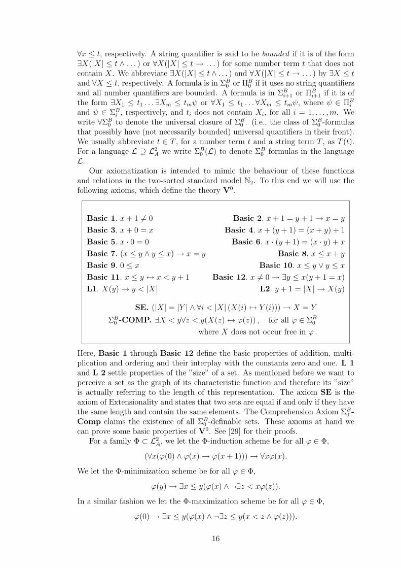
Here, Basic 1 through Basic 12 define the basic properties of addition, multi-plication and ordering and their interplay with the constants zero and one. L 1and L 2 settle properties of the ”size” of a set. As mentioned before we want toperceive a set as the graph of its characteristic function and therefore its ”size”is actually referring to the length of this representation. The axiom SE is theaxiom of Extensionality and states that two sets are equal if and only if they havethe same length and contain the same elements. The Comprehension Axiom ΣB

0 -Comp claims the existence of all ΣB

0 -definable sets. These axioms at hand wecan prove some basic properties of V0. See [29] for their proofs.

For a family Φ ⊂ L2A, we let the Φ-induction scheme be for all ϕ ∈ Φ,

(∀x(ϕ(0) ∧ ϕ(x)→ ϕ(x+ 1)))→ ∀xϕ(x).

We let the Φ-minimization scheme be for all ϕ ∈ Φ,

ϕ(y)→ ∃x ≤ y(ϕ(x) ∧ ¬∃z < xϕ(z)).

In a similar fashion we let the Φ-maximization scheme be for all ϕ ∈ Φ,

ϕ(0)→ ∃x ≤ y(ϕ(x) ∧ ¬∃z ≤ y(x < z ∧ ϕ(z))).

16

Proposition 1.26. V0 proves the ΣB0 -induction scheme, the ΣB

0 -minimizationscheme and the ΣB

0 -maximization scheme.

Also, V0, if restricted to its number part does not prove more than I∆0. Thefollowing theorem holds.

Proposition 1.27. V0 is a conservative extension of I∆0.

We can extend Parikh’s Theorem to the two-sorted case. To this end we first

Theorem 1.28 (Parikh, two-sorted). Let T be a two-sorted, polynomially bound-ed theory extending V0 and ϕ(x, y, X, Y ) be a bounded formula with all variablesshown. Then, if

T ⊢ ∀x∀X∃y∃Y ϕ(x, y, X, Y ),

it also holds thatT ⊢ ∀x∀X∃y ≤ t∃Y ≤ tϕ(x, y, X, Y ),

where t is a bounded term containing only the variables x, X.

Definable Relations and Functions

We will now give some V0-definable functions and relations that we need for ourarguments. For their proper definitions as well as for a thorough treatment of thenotion of definability with respect to V0, we refer the reader to Section A.2.1 inAppendix A.

If a relation R is ΣB0 -definable in V0, then so is its characteristic function χR.

We can define sequences of constant length of numbers by a standard encodingas numbers. We will denote such sequences by 〈x1, . . . , xk〉, where the xi arethe elements and k is a fixed standard number. We can also code sequences ofnumbers, which are not of constant length. Informally, the ΣB

0 -formula seq(i, Z),defined by Formula (A.9) in Appendix A, returns the ith element of the sequencecoded by Z. For brevity we will use Z[i] to refer to the ith element in the sequencecoded by Z. This encoding is not unique, but we can make it unique, by ensuringthat we talk about the lexicographically smallest Z encoding the sequence. Wewill refer to this encoding by Formula (A.10) and call the formula SEQ(i, Z).Thus, we can also refer to the length of a sequence by using a ΣB

0 -formula, whichwe call length(Z). This also allows us to define higher dimensional sequences ofnumbers, i.e. matrices, etc. We will refer to these elements as Z[i1, . . . , ik] and tolower dimensional subsequences in the same way, using · to represent the places,where the variable is still free. For example we refer to the first row in the matrixZ[i, j] by Z[1, ·]. This also gives us a means of encoding a sequence of strings, asit is essentially the same. There is a general way of extending the language L2

A

with new relation and function symbols, such that the theory extending V0 bydefining axioms of the symbols in the extended language, still has comprehensionand induction for the new statements and is conservative over V0. See SectionV.4 in [29] or, for a brief review, Section A.2.1 in Appendix A.

In the following two sections we will briefly review two extensions of V0 thatare subject to the later research. We focus only on the properties that are nec-essary for our results. See Appendix A or [29] for a more thorough treatment ofVTC0 and [29] for one on VNCk.

17

1.3.1 The Theory VTC0

The theory VTC0 is an extension of V0 by an axiom that ensures that we areable to count the size of strings. As we are not able to prove the PigeonholePrinciple in V0, the theory resulting from the addition of the axiom is properlystronger. Formally we let VTC0 consist of the theory V0 together with the axiomNUMONES defined as follows:

Definition 1.29 (NUMONES). Let δNUM(y,X, Z) be the following ΣB0 formula:

δNUM(y,X, Z) := SEQ(y, Z) ∧ Z[0] = 0 ∧ ∀u < y((X(u)→ Z[u+ 1] = Z[u] + 1)

∧ (¬X(u)→ Z[u+ 1] = Z[u])).

(1.1)

Define NUMONES to be the following ΣB1 formula:

NUMONES := ∃Z ≤ 1 + 〈y, y〉.δNUM(y,X, Z). (1.2)

Thus, NUMONES basically guarantees the existence of a sequence whichcounts the number of 1’s in a given string, that is, it measures the size of thebounded set related to that string.

Using NUMONES we can define the function numones(y,X) that, given y andX, returns the yth entry of Z(X) via the following ΣB

1 -defining axiom

numones(y,X) = z ↔ ∃Z ≤ 1+〈|X| , |X|〉 (δNUM(|X| , X, Z) ∧ Z[y] = z) . (1.3)

We shall use the following abbreviation:

numones(X) := numones(|X| − 1, X).

This axiom not only allows to count the number of elements of a set, butalso gives us the means to compute sums with a moderately large number ofsummands, as well as the product of two large numbers. Much like for V0, wecan also extend VTC0 in a conservative way by defining axioms for symbols in anextended language. The function numones can be introduced like this and we willmake use of such introduction several times to obtain a more convenient theoryfor the task at hand. See Section A.2.2 in Appendix A and also Sections I.X.3.2and I.X.3.3 in [29]. We will start out by describing how to do basic Linear Algebrain VTC0.

Some Elementary Linear Algebra in VTC0

Observe that proper Linear Algebra is well beyond the scope of TC0 and thatis even more the case when investigating the related theory VTC0. Therefore,what we will introduce here can only be considered as the very basics of LinearAlgebra. For a more thorough treatment of Linear Algebra, we would need tostrengthen the theory (see [89] for this). Using the pairing function availablein V0, we can code a subset of the rational numbers, more precisely we code anumber x

yas the pair 〈x, y〉. The numbers we will be working with will all have

a common denominator n2c. This limits the number of multiplications we can dofor each number, but this will not pose a problem in our case. We can also define

18

the usual operations on these numbers (see for example [69]). Given a string Zcoding a sequence, we can compute the value of the sum of its elements, thatis, we can ΣB

1 -define a formula sum(y, Z) that represents∑y

i=0 Z[i] and prove itsmain properties as well as its totality in VTC0 (see Proposition 1.30 below orProposition A.39 in Appendix A for the proof). We define rational vectors in anatural way as sequences of rational numbers. Using the sum function we candefine an inner product of vectors of the same length. For vectors ~u,~v ∈ Qk wedenote the inner product by 〈~u,~v〉. For a rational matrix M and a rational vector~v, we can ΣB

1 -define their product M~v.

Proposition 1.30 (Basic properties of sums in VTC0). In what follows weconsider the theory VTC0 over an extended language (including possibly newΣB

1 -definable function symbols in VTC0 and their defining axioms). The functionf(i) is a number function symbol mapping to the rationals or naturals (possiblywith additional undisplayed parameters). The theory VTC0 proves the followingstatements:

Substitution: Assume that u(i), v(i) are two terms (possibly with additionalundisplayed parameters), such that u(i) = v(i) for any i ≤ n, then

n∑

i=0

f(u(i)) =n∑

i=0

f(v(i)).

Distributivity: Assume that u is a term that does not contain the variable i,then

u ·n∑

i=0

f(i) =n∑

i=0

u · f(i).

Rearranging: Assume that I = 0, . . . , n and let I1, . . . , Ik be a definable par-tition of I (specifically, the sets I1, . . . , Ik are all ΣB

0 -definable in VTC0 andVTC0 proves that the Ij’s form a partition of I). Then

n∑

i=0

f(i) =k∑

j=1

∑

i∈Ij

f(i),

where∑

i∈Ijf(i) denotes the term

∑|Ij |−1i=0 f(δ(i)) where δ(i) is the function

that enumerates (in ascending order) the elements in Ij.

Inequalities: Let g(i) be a number function mapping to the rationals or naturals(possibly with additional undisplayed parameters), such that f(i) ≤ g(i) forall 0 ≤ i ≤ n, then

n∑

i=0

f(i) ≤n∑

i=0

g(i).

Additionally to being able to compute the sizes of bounded sets, we can al-so prove some elementary counting properties. We will now give a synopsis ofSection A.2.2 in Appendix A and refer to that section for the proofs.

Notation: When reasoning in the theory VTC0, we will say that a family ofΣB

0 -definable in VTC0 sets B0, . . . , Bℓ forms a partition of a set B whenever

19

VTC0 proves that (i)⋃ℓ

i=0Bi = B, and (ii) Bi ∩ Bj = ∅, for all 0 ≤ i 6= j ≤ ℓ.

Here,⋃ℓ

i=0Bi := r : ∃i ≤ ℓ, Bi(r).

Proposition 1.31 (Some counting in VTC0). Let B1, . . . , Bℓ be family of ΣB0 -

definable sets in VTC0 that partition the set B (ℓ may be a variable). Then,VTC0 proves:

numones(B) =ℓ∑

i=1

numones(Bi) .

Proposition 1.32 (More counting in VTC0). Let ϕ(x) be a ΣB0 formula (pos-

sibly in an extended language of VTC0). The theory VTC0 can prove that ifZ = 0 ≤ i < m : ϕ(i) and for any 0 ≤ i < m,

γi =

a, ϕ(i);b, ¬ϕ(i),

then ∑

i<m

γi = a · numones(Z) + b · (m− numones(Z)).

For a number term t, we write ∀x ∈ [t] Φ to abbreviate ∀x ≤ t(x ≥ 1→ Φ).

Proposition 1.33. The theory VTC0 proves the following statement. Let F (x)be a string function. Let d < t be a natural number and assume that any numberin any set F (1), . . . , F (t) occurs in at most d many sets in F (1), . . . , F (t). Letg(x) be a number function such that g(1), . . . , g(t) are (not necessarily distinct)numbers with g(i) ∈ F (i) for all i ∈ [t]. Then numones(g(i) : i ∈ [t]) ≥ ⌈t/d⌉.

1.3.2 The Theories VNCk and VNC

As before we will axiomatize theories corresponding to the provability strengthof circuit classes by adding to V0 an axiom that postulates the existence of awitness for a complete problem for that circuit class. In this section we will treatNCk circuits and, following [29], we will use the layered monotone circuit valueproblem, which is complete for these classes, to axiomatize the correspondingtheories VNCk. We will be more precise now.

Definition 1.34. The monotone circuit value problem for some circuit class Cis, given a monotone circuit C ∈ C and an input I to C, to decide whetherC(I) = 1 or not. The layered monotone circuit value problem is the same forlayered circuits.

These problems are hard for their respective classes.

Proposition 1.35. Let k ≥ 0. The layered and non-layered monotone circuitvalue problems for ACk and NCk+1 are hard for the classes ACk and NCk+1, re-spectively.

We will now formalize these problems. To do so, we will first consider thecase where k = 1. In this case any NCk-circuit can efficiently be turned into an

20

equivalent formula. The circuit value problem thus reduces to a formula valueproblem, which is the base of the following definition of VNC1.

We perceive a monotone formula ϕ as a encoded by a binary tree G, wherethe leafs are labeled with the variables and each node is labeled by a connective,i.e. by either ∧ or ∨. An assignment is a string I, that assigns to each variable avalue, i.e. 0 or 1. The following formula is a formalization of the statement thatthere exists an evaluation Y for each such encoding of a formula:

MFV ≡ ∃Y ≤ 2a+ 1.δMFV (a,G, I, Y ), where

δMFV (a,G, I, Y ) ≡ ∀x < a((Y (x+ a)↔ I(x)) ∧ Y (0)∧0 < x→ (Y (x)↔ ((G(x) ∧ Y (2x) ∧ Y (2x+ 1))∨

(¬G(x) ∧ (Y (2x) ∨ Y (2x+ 1)))))).

Definition 1.36. We let VNC1 be V0 augmented by MFV .

To further generalize this notion we first need to find a convenient way offormalizing the notion of an ACk and of an NCk circuit. This is done as follows.

We define a circuit in L2A by defining the underlying set of nodes via a predicate

G[〈a, b〉] that is true iff the bth node in layer a is ∧ and false iff it is ∨. The nodesare connected via an edge relation E[〈a, b, c〉] that is true iff node b on layer a isconnected with node c on layer a+ 1.

The algorithm that we want to formalize, starts in the lowest layer and com-putes the values of each node in this layer from the input I it then successivelycomputes the values of all nodes in each layer from the layer below. Therefore itneeds space O(size of the layer) and can be formalized as follows.

δLMCV (n, d, E,G, I, Y ) ≡ ∀x < n∀z < d((Y [〈0, x〉]↔ I[x]))∧(Y [〈z + 1, x〉]↔(G[〈z + 1, x〉] ∧ ∀u < n(E(z, u, x)→ Y (z, u)))∨(¬G[〈z + 1, x〉] ∧ ∃u < n(E(z, u, x)→ Y (z, u)))).

As the circuit we want to compute is an NC circuit we have to assume thatthe fan-in is 2. We formalize that as

Fanin2(n, d, E) ≡ ∀z < d∀x < n∃u1 < n∃u2 < n∀v < n

(E(z, v, x)→ (v = u1 ∨ v = u2)).

We are now in the position to define the theories that correspond to the circuitclasses NCk.

Definition 1.37. Let k > 1. Then VNCk is axiomatized by V0 extended bythe following axiom

Fanin2(n, |n|k , E)→ ∃Y ≤ 〈|n|k , n〉δLMCV (n, |n|k , E,G, I, Y )

The theory VNC is defined by adding the above axiom for all k.

21

Obviously the theories form a hierarchy, though we do not know, whether itis strict.

Observe that none of the VNCk is conservative over V0, as, by the WitnessingTheorem for V0, a ΣB

0 definition of the satisfaction relation would be sufficientto prove that NC1 ⊆ AC0, at least for monotone functions, which is known to befalse.

The theories VNCk are at least as strong as VTC0. See [29] Section IX.5.4.

Theorem 1.38. VNC1 proves NUMONES. Therefore everything provable inVTC0 is also provable in VNCk for any k ≥ 1.

1.3.3 Relation between Arithmetic Theories and ProofSystems

In this section we will remind the reader of a connection between the TheoryV0 and some of its extensions and certain propositional proof systems (see also[29][57]).

Definition 1.39. The following predicates will be subsequently used. They aredefinable with respect to V0 (see [57]).

• Fla(X) is a ΣB0 formula that says that the the string X codes a formula.

• DNF(X) is a ΣB0 formula that says that the the string X codes a formula

in DNF.

• Z |= X is the ∆B1 definable property that the truth assignment Z satisfies

the formula X.

• Taut(X) is the ΠB1 formula Fla(X) ∧ ∀Z ≤ t(|X|)Z |= X, where t is a

number term.

• PrfFd(Π, A) is a ΣB

0 definable predicate meaning Π is a depth d Frege prooffor A.

• PrfTC0−Fd

(Π, A) is a ΣB0 definable predicate meaning Π is a depth d TC0-

Frege proof for A.

• PrfF (Π, A) is a ΣB0 definable predicate meaning Π is a Frege proof for A.

We denote the depth by a formula coded by a string X by dp(X). This isclearly ΣB

0 definable in V0. Observe that in V0 we cannot prove that everyformula has an evaluation.

The following holds

Theorem 1.40 (see [29]). The Theory V0 proves that AC0-Frege is sound, i.e.for every d

∀A∀ΠPrfFd(Π, A) ∧ dp(A) ≤ d→ Taut(A).

Theorem 1.41 (see [29]). The Theory VTC0 proves that TC0-Frege is sound,i.e.

∀A∀ΠPrfTC0−Fd

(Π, A) ∧ dp(A) ≤ d→ Taut(A).

22

Theorem 1.42 (see [29]). The Theory VNC1 proves that Frege is sound, i.e.

∀A∀ΠPrfF (Π, A)→ Taut(A).

On the other hand, provability of the universal closure of ΣB0 formulas in V0

and VNC1 implies the existence of polynomial size proofs of their propositionaltranslations in AC0-Frege, TC0-Frege and Frege, respectively.

The Paris-Wilkie Translation

We will show now, how one can translate a ΣB0 formula ϕ into a family of proposi-

tional formulas JϕK and use this translation to infer a relation between provabilityin V0 and its extensions to efficient provability in bounded depth Frege, TC0-Fregeand Frege. This is the Paris-Wilkie Translation defined in [73].

Definition 1.43 (Propositional translation J·K of ΣB0 formulas). Let ϕ(x, X) be

a ΣB0 formula. The propositional translation of ϕ is a family

JϕK = JϕKm;n | mi, ni ∈ N

of propositional formulas in variables pXi

j for everyXi ∈ X. The intended meaningis that JϕK is a valid family of formulas if and only if the formula

∀x∀X((∧|Xi| = ni)→ ϕ(m, X)

)

is true in the standard model N2 of two sorted arithmetic, where n denotes thenth numeral, for any n ∈ N.

For given m, n ∈ N we define JϕK by induction on the size of the formulaJϕKm;n. We denote the value of a term t by val(t).

Case 1: Let ϕ(x, X) be an atomic formula.

• If ϕ(x, X) is ⊤ (or ⊥), then JϕKm,n := ⊤ (or ⊥).

• If ϕ(x, X) is Xi = Xi, then JϕKm,n := ⊤.

• If ϕ(x, X) is Xi = Xj for i 6= j, then (using the fact that V0contains theextensionality axiom SE) instead of translating ϕ, we translate the V0-equivalent formula

|Xi| = |Xj| ∧ ∀k ≤ |X| (Xi(k)↔ Xj(k))).

• If ϕ(x, X) is t1(y, |Y |) = t2(z, |Z|) for terms t1, t2, number variables y, z andstring variables Y , Z, where y ∪ z = x and Y ∪ Z = X, and my, mz andnY , nZ denote the corresponding assignments of numerals m, n to the y, zand Y , Z variables, respectively. Then

JϕKm,n :=

⊤ if val(t1(m

Y , nY )) = val(t2(mZ , nZ)) and

⊥ otherwise.

23

• If ϕ(x, X) is t1(y, |Y |) ≤ t2(z, |Z|) for terms t1, t2, number variables y, z andstring variables Y , Z, then

JϕKm,n :=

⊤ if val(t1(m

Y , nY )) ≤ val(t2(mZ , nZ)) and

⊥ otherwise.

• If ϕ(x, X) is Xi(t(x, |X|)), then

JϕKm,n := ⊥ if ni = 0

and otherwise

JϕKm,n :=

pXi

val(t(m,n)) if val(t(m, n)) < ni − 1,

⊤ if val(t(m, n)) = ni − 1,

⊥ if val(t(m, n)) > ni − 1.

Case 2: The formula ϕ is not atomic.

• If ϕ ≡ ψ1 ∧ ψ2 we let

JϕKm,n := Jψ1Km,n ∧ Jψ2Km,n.

• If ϕ ≡ ψ1 ∨ ψ2 we let

JϕKm,n := Jψ1Km,n ∨ Jψ2Km,n.

• If ϕ ≡ ¬ψ we letJϕKm,n := ¬JψKm,n.

• If ϕ ≡ ∃y ≤ t(x, |X|)ψ(y, x, X) then

JϕKm,n :=

val(t(m,n))∨

i=0

Jψ(i, x, X)Km,n.

• If ϕ ≡ ∀y ≤ t(x, |X|)ψ(y, x, X) then

JϕKm,n :=

val(t(m,n))∧

i=0

Jψ(i, x, X)Km,n.

This concludes the translation for ΣB0 formulas.

Proposition 1.44. There exists a polynomial p such that for all ΣB0 formulas

ϕ(x, X) the following holds

• If V0 ⊢ ∀X∀xϕ(x, X), then there exist a d such that all JϕKm,n have depthd Frege proofs of length at most p(max(m, n)), for any m, n.

• If VTC0 ⊢ ∀X∀xϕ(x, X), then there exist a d such that all JϕKm,n havedepth d TC0-Frege proofs of length at most p(max(m, n)), for any m, n.

24

• If VNC1 ⊢ ∀X∀xϕ(x, X), then there exist Frege proofs of all JϕKm,n oflength at most p(max(m, n)), for any m, n.

Propositions 1.40, 1.41 and 1.42 are examples of general principles, the socalled Reflection Principles, which we will state now only for formulas in DNF,as V0 is not strong enough to evaluate general formulas.

Definition 1.45 (Reflection Principle). Let P be a pps. Then the ReflectionPrinciple for P , RefP , is the ∀∆B

1 -formula (w.r.t. V0)

∀Π∀X∀Z((DNF(X) ∧ PrfP (Π, X))→ (Z X)),

where PrfP is a ∆B1 -predicate formalizing P -proofs.

Reflection Principles condense the strength of propositional proof systems.The following result exemplifies this. A detailed exposition can be found in [29],chapter X, or in [57], chapter 9.3.

Theorem 1.46. 1. If V0 ⊢ RefF then bounded depth Frege simulates Fregew.r.t. DNF formulas.

2. If V0 ⊢ RefTC0−F then bounded depth Frege simulates TC0-Frege w.r.t. DNF

formulas.

3. If VTC0 ⊢ RefF then TC0-Frege simulates Frege w.r.t. DNF formulas.

We will only give a brief sketch of the proof of item 1. here and leave out thetechnical details.

Sketch. Let ϕ be a formula and πϕ a Frege proof of ϕ. Since V0 proves RefF ,by Propositions 1.40 and 1.44 we have polynomial size proofs of its translationsJRefF K in bounded depth Frege. Bounded depth Frege itself, however, is strongenough to verify that a proper encoding of the computation of the Turing machineverifying the Frege proof πϕ is correct. Thus it can verify that πϕ is a Frege-proofand, using the translation of the Reflection Principle and the Cut rule, concludeJTaut(ϕ)K. From this ϕ follows, cf. [57] Lemma 9.3.7.

As an application of Theorem 1.46 we can state the following observation.

Proposition 1.47. VTC0 is not a conservative extension of V0.

Proof. This statement follows from Theorem 1.9 and Theorem 1.14. If V0 couldprove the same statements as VTC0, then, by Proposition 1.41, it could especial-ly prove the Reflection Principle for TC0-Frege. This, in conjunction with The-orem 1.14 and Proposition 1.44 yields a polynomially bounded, bounded depthFrege proof of the Pigeonhole Principle. That, however, is a contradiction toTheorem 1.9.

25

2. Refutations of Random 3CNFin TC

0-Frege

In this chapter we will give a synopsis of [67], the whole article is given as Ap-pendix A in the end of the thesis.

By Theorem 1.5 we know that Resolution fails to have efficient proofs of theunsatisfiability of random 3CNF, if the clause-to-variable ratio is below n0,5−ǫ,where n is the number of variables. This is contrasted by Theorem 1.4, whichstates that these statements are already well beyond the unsatisfiability thresholdof 8·ln(2) clauses per variable, which suggests that proofs of unsatisfiability shouldbe easier to do. This suggestion is justified. In [37], Feige, Kim and Ofek showedthat there is a polynomially verifiable witness of the unsatisfiability of 3CNF, ifthe clause-to-variable ratio is at least c · n0,4 for some constant c. This is ourstarting point. We will show that this witness can be understood with the meansof TC0-Frege and then conclude that 3CNF with more than c · n0,4 clauses pervariable can be efficiently refuted by TC0-Frege proofs (by which we mean thatTC0-Frege proves their negation efficiently). Our main result is the following:

Theorem 2.1. With probability 1−o(1) a random 3CNF formula with n variablesand cn1.4 clauses (for a sufficiently large constant c) has polynomial-size TC0-Frege refutations.

We will now give an outline of the structure of the proof of Theorem 2.1. In-stead of directly constructing TC0-Frege proofs we will work in VTC0 and use therelation between this theory and the proof system, as mentioned in Section 1.3.3.We have seen there that, when restricted to proving ΣB

0 statements, the theoryVTC0 characterizes uniform polynomial-size TC0-Frege proofs. The constructionof polynomial-size TC0-Frege refutations for random 3CNF formulas, will consistof the following steps:

I. Formalize the following statement as an L2A formula:

∀ assignment A(C is a 3CNF and w is its FKO unsatisfiabiliy witness −→

exists a clause Ci in C such that Ci(A) = 0),

(2.1)

where an FKO witness is a suitable formalization of the unsatisfiabilitywitness defined by Feige, Kim and Ofek [37]. We will call the correspondingpredicate the FKO predicate.

II. Prove formula (2.1) in the theory VTC0.

III. Translate the proof in Step II. into a family of propositional TC0-Frege proofs(of the family of propositional translations of (2.1)). By Proposition 1.44,this will be a polynomial-size propositional proof (in the size of C). Thetranslation of (2.1) will consist of a family of propositional formulas of theform:

JC is a 3CNF and w is its FKO unsatisfiabiliy witnessK −→Jexists a clause Ci in C such that Ci(A) = 0K.

(2.2)

26

By the nature of the propositional translation, (second-sort) variables inthe original first-order formula translate into a collection of propositionalvariables. Thus, (2.2) will consist of propositional variables derived fromthe variables in (2.1).

IV. For the next step we first notice the following two facts:

(i) Assume that C is a random 3CNF with n variables and cn1.4 clauses(for a sufficiently large constant c). By [37], with high probabilitythere exists an FKO unsatisfiability witness w for C. Both w and Ccan be encoded as finite sets of numbers, as required by the predicatefor 3CNF and the FKO predicate in (2.1). Let us identify w and Cwith their encodings. Then, assuming (2.1) was formalized correctly,assigning w and C to (2.1) satisfies the premise of the implication in(2.1).

(ii) Now, by the definition of the translation from first-order formulas topropositional formulas, if an object α satisfies the predicate P (X)(i.e., P (α) is true in the standard model), then there is a propositionalassignment of 0, 1 values that satisfies the propositional translation ofP (X). Thus, by Item (i) above, there exists an 0, 1 assignment ζ thatsatisfies the premise of (2.2) (i.e., the propositional translation of thepremise of the implication in (2.1)).

In the current step we show that after assigning ζ to the conclusion of (2.2)(i.e., to the propositional translation of the conclusion in (2.1)) one obtainsprecisely ¬C (formally, a renaming of ¬C, where ¬C is the 3DNF obtainedby negating C and using the de Morgan laws).

V. Take the propositional proof obtained in III., and apply the assignment ζ toit. The proof then becomes a polynomial-size TC0-Frege proof of a formulaφ → ¬C, where φ is a propositional sentence (without variables) logicallyequivalent to True (because ζ satisfies it, by IV.) From this, one can easilyobtain a polynomial-size TC0-Frege refutation of C (or equivalently, a proofof ¬C).

The bulk of our work lies in I. and especially in II. We need to formalize thenecessary properties used in proving the correctness of the FKO witnesses andshow that the correctness argument can be carried out in the weak theory. Thereare two main obstacles in this process. The first obstacle is that the correctness(soundness) of the witness is originally proved using spectral methods, whichassumes that eigenvalues and eigenvectors are over the reals ; whereas the realsare not defined in our weak theory. The second obstacle is that one needs to provethe correctness of the witness, and in particular the part related to the spectralmethod, constructively (formally in our case, inside VTC0). Specifically, linearalgebra is not known to be (computationally) in TC0, and (proof-complexity-wise)it is conjectured that TC0-Frege do not admit short proofs of the statements oflinear algebra (more specifically still, short proofs relating to inverse matrices andthe determinant properties; see [89] on this).

27

The first obstacle is solved using rational approximations of sufficient accu-racy (polynomially small errors), and showing how to carry out the proof in thetheory with such approximations. The second obstacle is solved basically byconstructing the argument (the main formula above) in a way that exploits non-determinism (i.e., in a way that enables supplying additional witnesses for theproperties needed to prove the correctness of the original witness; e.g, (approxi-mations of) all eigenvectors and all eigenvalues of the appropriate matrices in theoriginal witness). In other words, we do not have to construct certain objects butcan provide them, given the possibility to certify the property we need. Formally,this means that we put additional witnesses in the FKO predicate occurring inthe main formula in I. above. This, of course, leads to TC0-proofs that are nottotally uniform.

We will now elaborate a bit more on Steps I. and II.

2.0.4 Step I.

To understand how to formalize the notion of an FKO witness, we first have todefine what that notion actually is. In [37] the following was observed

1. Any satisfying assignment for a random 3CNF C satisfies many clauses ofC as 3XOR, that is, it either satisfies all or exactly one of the literals inthese clauses.

2. Not too many of the clauses of C can be satisfied as NAE (Not All Equal),that is there are a reasonable amount of clauses, where all 3 literals aresatisfied.

3. For any random 3CNF, there exist many distinct, but not disjoint sets oftheir clauses, such that each of this sets one of its clauses is not satisfied as3XOR.

If there exists too many of the sets guaranteed by item 3, we cannot satisfy item1 anymore, so the 3CNF is not satisfiable. We will make this observation moreprecise now.

We call the collection of clauses in item 3) an even k-tuple and define it asfollows

Definition 2.2 (Even k-tuple). For any given k, a sequence S of k many clausesis an even k-tuple iff every variable appears an even number of times in thesequence. Formally, this predicate is denoted by TPL(S, k).

Observe that if S is an even k-tuple then k is even (since the total number ofvariable occurrences n is even, by assumption that each variable occurs an evennumber of times; and k = n/3, since each clause has three variables). In light ofthe fact that many clauses have to be satisfied as 3XOR (item 1. in the aboveobservation), we define the following:

Definition 2.3 (Inconsistent k-tuple). An even k-tuple is said to be inconsistentif the total number of negations in its clauses is odd. Formally, the predicate isdenoted by ITPL(S, k).

28

Observe that at least one of the clauses in an inconsistent k-tuple cannot besatisfied as 3XOR. Additionally, we need the the largest eigenvalue λ of thefollowing matrix, because it provides an upper bound to the number of clausesthat can be satisfied as NAE (item 2 above).

Definition 2.4 (Mat(M,C)). We define the predicate Mat(M,C) that holdsiff M is an n × n rational matrix such that Mij equals 1

2times the number of

clauses in C where xi and xj appear with different polarity minus 12

times thenumber of clauses where they appear with the same polarity. More formally, wehave

Mij :=m−1∑

k=0

E(k)ij , for any i, j ∈ [n], (2.3)

where E(k)ij corresponds to the kth clause in C as follows:

E(k)ij :=

12, xεi

i , xεj

j ∈ C[k] and εi 6= εj, for some εi, εj ∈ 0, 1 and i 6= j;−1

2, xεi

i , xεj

j ∈ C[k] and εi = εj, for some εi, εj ∈ 0, 1 and i 6= j;0, otherwise.

(2.4)

We refer to Lemma 2.11 for the actual bound of the formulas satisfied asNAE. Also, the eigenvalue λ poses a problem as on the one-hand, the eigenval-ue is a real number and on the other hand, we cannot construct eigenvalues inour theory, even if they are rational. To circumvent this, we define a predicateEigValBound(M, λ, V ) that ensures that λ is a collection of n rational approx-imations of the eigenvalues of the matrix M and that V is the rational matrixwhose rows are the rational approximations of the eigenvectors of M (where theith row in V is the approximation of the approximate eigenvector λi).

The notion of imbalance provides us with a natural upper bound for the totalnumber of satisfied literals.

Definition 2.5 (The imbalance Imb(C, y)). For a 3CNF C we define the functioni-imbalance iImb(C, i) to be the absolute value of the difference of negated occur-rences of xi and non-negated occurrences of xi in the 3CNF C (where x1, . . . , xn

are considered to be all the variables in C). It is denoted by iImb(C, i). For a3CNF C, the predicate imbalance of C, denoted Imb(C, y), is true iff y equalsthe sum over the i-imbalances of all the variables, that is:

Imb(S, y)↔ y =n∑

i=1

iImb(C, i).

We can now formulate the witness and give a sketch of the proof of its correct-ness. But first, we need one more definition, which gives a bound to the numberof inconsistent k-tuples (as for item 3):

Definition 2.6 ((t, k, d)-collection). A (t, k, d)-collection D of a 3CNF C withm clauses is an array of t many inconsistent k-tuples, which contain only clausesfrom C, and each clause appears in at most d many such inconsistent k-tuples.The predicate is denoted Coll(t, k, d,C,D).

The witness for unsatisfiability of C contains

29

• The imbalance I given as Imb(C, y),

• the largest eigenvalue λ from Mat(M,C) and

• a (t, k, d)-collection Coll(t, k, d,C,D).

Before we will state the main formula, we will restate the result from [37] of howthe witness is applied.

Theorem 2.7 ([37]). Let C be a 3CNF with n variables and m clauses and the

FKO witness as above. If t > d·(I+λn)2

, then C is not satisfiable.

We can now present the main formula that we are going to prove in VTC0.It says that if the Feige-Kim-Ofek witness fulfills the inequality t > d·(I+λn)

2+o(1)

(the o(1) stems from the approximations) then there exists a clause in C that isnot satisfied by any assignment A (the predicate NotSAT(C[i], A) is a straight-forward formalization of this property):

Definition 2.8 (The main formula). The main formula is the following formula(λ denotes n distinct number parameters λ1, . . . , λn):

(3CNF(C, n,m) ∧Coll(t, k, d,C,D) ∧ Imb(C, I) ∧Mat(M,C)∧

EigValBound(M, λ, V ) ∧ λ = maxλ1, . . . , λn ∧ t >d · (I + λn)

2+ o(1)

)

−→ ∃i < mNotSAT(C[i], A).

2.0.5 Step II.

The proof of the main formula in VTC0 is rather tedious, so we will only givethe main results needed to follow it and refer to the appendix for the details.

Theorem 2.9 (Main). The theory VTC0 proves the main formula (Definition2.8).

We will give a very brief sketch of the argument. The proof uses the followinglemmas, the proofs of which can be found in Appendix A:

Let satNAE(A,C) be the string function that returns the set of all clauses inC that are satisfied as NAE by A and satLit(A,C) the set of all literals that aresatisfied by A.

Lemma 2.10 (Lemma A.50 in Appendix A). (Assuming the premise of the mainformula) the theory VTC0 proves:

numones(satLit(A,C)) ≤ 3m+ I

2.

30

Lemma 2.11 (Lemma A.55 in Appendix A). (Assuming the premise of the mainformula) the theory VTC0 proves:

numones(satNAE(A,C)) ≤ (nλ+ 3m)/4 + o(1).

Lemma 2.12 (Lemma A.56 in Appendix A). (Assuming the premise of the mainformula) the theory VTC0 proves that the number of clauses in C that are notsatisfied as 3XOR by A is at least ⌈t/d⌉.

Proof of Theorem 2.9. We will argue in VTC0. Assume that the premise of themain formula (see Definition 2.8) holds. By Lemma 2.10 the maximal number ofliterals satisfied by the assignment A is

3m+ I

2.

By Lemma 2.11 at mostnλ+ 3m

4+ o(1)

clauses are satisfied as NAE. The remaining (m− nλ+3m4

+ o(1)) clauses must besatisfied 3 times. Thus the number of clauses satisfied twice is at most

3m+ I

2− 3 · (m− nλ+ 3m

4)

︸ ︷︷ ︸satisfied 3 times

− nλ+ 3m

4︸ ︷︷ ︸satisfied once

+o(1) =−3m+ I

2+nλ+ 3m

2+ o(1)

=nλ+ I

2+ o(1).

On the other hand, by Lemma 2.12, this number is at least ⌈t/d⌉. Thus we get

t ≤ d · ⌈t/d⌉ ≤ d · (nλ+ I)

2+ o(1),

contradicting the premise

t >d · (I + λn)

2+ o(1).

31

3. Cuts of Models of V0

In this chapter we will give a synopsis of [66]. The full version including theproofs is given as Appendix B in the end of this thesis.

In Section 3.1, we will reproduce the main argument of the article and concludea simulation result by exploiting an algorithm for evaluating formulas. We willgive a strengthened simulation result in Section 3.2, which builds on a differentalgorithm that evaluates general monotone circuits. The main result of [66] is theproof of a formalized version of Nepomnjascij’s Theorem [68] in a small cut of amodel of V0. The theorem is as follows:

Theorem 3.1 (Nepomnjascij [68]). Let c ∈ N and 0 < ǫ < 1 be constants.Then if the language L ∈ TimeSpace(nc, nǫ), the relation x ∈ L is definable by aΣB

0 -formula over N.

Using a standard evaluation algorithm the formalized version of this theoremguarantees the ΣB

0 -definability of MFV in the cut. This guarantees the existenceof an evaluation, i.e. it shows that the cut is a model of VNC1. In Section 3.2we will strengthen this latter result in a straightforward way to obtain a model ofVNC. In both cases that implies a subexponential simulation result with respectto the proof systems related to the theories. We will now introduce the notion ofa cut I of a given two-sorted arithmetic modelM.

Definition 3.2 (Cut). Let T be a two-sorted arithmetic theory and

N = N1, N2,+N , ·N ,≤N , 0N , 1N , |·|N ,=N

1 ,=N2 ,∈N

a model of T . A cut

M = M1,M2,+M , ·M ,≤M , 0M , 1M , |·|M ,=M

1 ,=M2 ,∈M

in N is any substructure such that

• M1 ⊆ N1, M2 ⊆ N2,

• 0M = 0N , 1M = 1N ,

• M1 is closed under +N , ·N and downwards with respect to ≤N ,

• M2 = X ∈ N2 | X ⊆M1, and

• M is the restriction of N to M1 and M2 for all relation and functionsymbols ∈ L2

A.

We call this cut the Polylogarithmic Cut iff

x ∈M1 ⇔ ∃a ∈ N1, k ∈ N x ≤ |a|k .

32

3.1 Polylogarithmic Cuts and VNC1

To infer the simulation result, we need a bounded version of the Reflection Prin-ciples we have defined in Section 1.3.3.

Given a term t and a variable x, we can also introduce the t-bounded versionof the Reflection Principle for some given pps P , RefP (t(x)) that claims soundnessonly for t-bounded proofs.

Definition 3.3 (Bounded Reflection). Let t be a L2Ar-term, x a first-sort variable

and P a pps. Then the Bounded Reflection Principle RefP (t(x)) is the formula

∀Π ≤ t(x)∀X ≤ t(x)∀Z ≤ t(x)((Fla(X) ∧ PrfP (Π, X))→ (Z X)).

We can now generalize Theorem 1.46 in the following way.

Theorem 3.4. Let t be a L2A-term and m a number variable. If t(m) < m for

m large enough and if V0 ⊢ ∀xRefF (t(x)) then for every propositional formulaϕ with a Frege proof of length t(m) there is a bounded depth Frege proof of ϕ oflength mO(1).

The following corollary will be of interest to us.

Corollary 3.5. If V0 ⊢ RefF (|x|k) for all k ∈ N, then bounded depth Frege subexponentially simulates Frege: For all D > 1, δ > 0 exists d ≥ D, such that theexistence of a Frege proof of length n of a depth D formula implies the existenceof a depth d Frege proof of length at most 2nδ

.

Given a polynomially bounded Turing machine A in a binary encoding, wecan ΣB

1 define a predicate ACCA(X), that states that X is accepted by A. Thiscan readily be observed, since, provided some machine A, there is a constantnumber of states σ1, . . . , σk and the whole computation can be written into amatrix W of polynomial size. We can also define a ΣB

1 -predicate REACHA(X,Y )that says that A reaches configuration Y from configuration X in at most p(|X|)steps. The definition is essentially the same as for ACC. The formalized versionof Nepomnjascij’s Theorem now says that ACCA(X) can be ΣB

0 -defined, if themachine A computes a language L ∈ TimeSpace(nc, nǫ) and the objects aresmall (i.e. lie in the polylogarithmic cut).

Theorem 3.6. Let N V0. Let m = |a| for some a ∈ N1 and let c, k ∈ N andǫ < 1. If L ∈ TimeSpace(mc,mǫ) is computed by Turing machine A, then thereexists a ΣB

0 definition in N of the ΣB1 -predicate ACCA on the interval [0,mk].

I.e. any Y ∈ L, bounded by mk is ΣB0 -definable in N and therefore exists in the

polylogarithmic cut of N .

Proof Sketch. We inductively on d define a ΣB0 relation reachd

A(I, p1, p2, cell, comp)that states that the p2th cell of the work tape of A, starting on configuration Iand computing for p1 ·md 1−ǫ

k steps via the computation comp is cell. As d dependsonly on A and k we will be doing this induction outside of the theory to constructd many formulas. We will then prove the above mentioned properties of reachA

by ΣB0 induction on p1.

33

It is then straightforward to prove by induction on the number of lines incomp that comp is uniquely defined by reach0

A. We let

Reach0A(I, p1, p2, cell) =def ∃comp < q(|I|) reach0

A(I, p1, p2, cell, comp),

where q is some polynomial depending on the encoding.Now proceed by inductively defining reachd

A and ReachdA. Again, we can prove

uniqueness of the computation by induction on the number of its lines and let

ReachdA(i, p1, p2, cell) =def ∃comp < q(|I|) reachd

A(i, p1, p2, cell, comp).

We now can give a ΣB0 definition of the predicate W [〈i, j, ·〉] coding the compu-

tation as in ACCA on input X of length mk. Informally the predicate W [〈i, j, ·〉]says that we compute the configurations of A by iteratively using the predicatesReachd

A through Reach0A. That is, we first exhaust applications of Reachd

A (i.e.we first make the biggest steps) until another application would lead us beyondthe configuration con we want to check. We can then use the configuration cond,that we obtained from the applications of Reachd

A, in Reachd−1A to get configura-

tion cond−1 and so on until we reach configuration con. It remains to check thatW [〈i, j, ·〉] coincides with the predicate ACCA. This follows by induction on thelength of the computation.

We can now conclude that such a cut is a model of VNC1 by providing analgorithm for formula evaluation. The algorithm can be found in the proof ofTheorem B.14 in Appendix B.

Theorem 3.7. Let N V0 and M ⊆ N be the polylogarithmic cut. ThenM VNC1.

Using the corollary to Theorem 3.4, this yields the following simulation resultfirst proved by Filmus, Pitassi and Santhanam [39].

Theorem 3.8 ([39]). Every Frege system is sub exponentially simulated by AC0-Frege systems.

As VNC1 extends VTC0, we can also infer the following result about boundeddepth Frege proofs of random 3CNF using Theorem 2.1 in Chapter 2.

Theorem 3.9. For almost every random 3CNF A with n variables and m = c·n1,4

clauses, where c is a large constant, ¬A has subexponentially bounded AC0-Fregeproofs.

This yields a weak separation result on random instances between Resolutionand bounded depth Frege.

3.2 Polylogarithmic Cuts and VNC

In this section we will generalize Theorem 3.7 in the sense that we show that thepolylogarithmic cut of any V0 model is actually a model of VNC instead of onlyVNC1. This result stems from discussions with Antonina Kolokolova in the SASprogramme in Cambridge and subsequently in Prague.

34

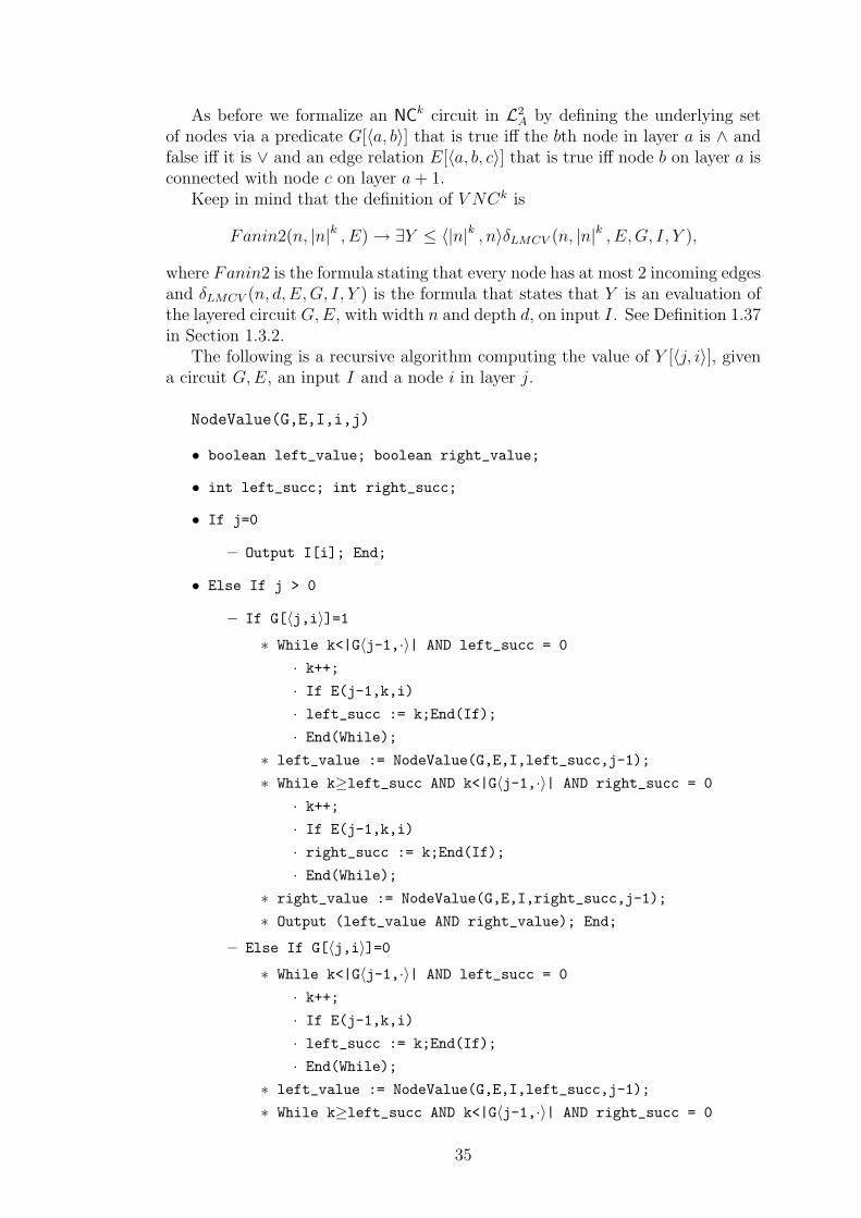
As before we formalize an NCk circuit in L2A by defining the underlying set

of nodes via a predicate G[〈a, b〉] that is true iff the bth node in layer a is ∧ andfalse iff it is ∨ and an edge relation E[〈a, b, c〉] that is true iff node b on layer a isconnected with node c on layer a+ 1.

Keep in mind that the definition of V NCk is

Fanin2(n, |n|k , E)→ ∃Y ≤ 〈|n|k , n〉δLMCV (n, |n|k , E,G, I, Y ),

where Fanin2 is the formula stating that every node has at most 2 incoming edgesand δLMCV (n, d, E,G, I, Y ) is the formula that states that Y is an evaluation ofthe layered circuit G,E, with width n and depth d, on input I. See Definition 1.37in Section 1.3.2.

The following is a recursive algorithm computing the value of Y [〈j, i〉], givena circuit G,E, an input I and a node i in layer j.

NodeValue(G,E,I,i,j)

• boolean left_value; boolean right_value;

• int left_succ; int right_succ;

• If j=0

– Output I[i]; End;

• Else If j > 0

– If G[〈j,i〉]=1∗ While k<|G〈j-1,·〉| AND left_succ = 0

· k++;· If E(j-1,k,i)

· left_succ := k;End(If);

· End(While);∗ left_value := NodeValue(G,E,I,left_succ,j-1);

∗ While k≥left_succ AND k<|G〈j-1,·〉| AND right_succ = 0

· k++;· If E(j-1,k,i)

· right_succ := k;End(If);

· End(While);∗ right_value := NodeValue(G,E,I,right_succ,j-1);

∗ Output (left_value AND right_value); End;

– Else If G[〈j,i〉]=0∗ While k<|G〈j-1,·〉| AND left_succ = 0

· k++;· If E(j-1,k,i)

· left_succ := k;End(If);

· End(While);∗ left_value := NodeValue(G,E,I,left_succ,j-1);

∗ While k≥left_succ AND k<|G〈j-1,·〉| AND right_succ = 0

35

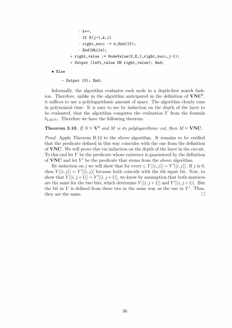
· k++;· If E(j-1,k,i)

· right_succ := k;End(If);

· End(While);∗ right_value := NodeValue(G,E,I,right_succ,j-1);

∗ Output (left_value OR right_value); End;

• Else

– Output (0); End;

Informally, the algorithm evaluates each node in a depth-first search fash-ion. Therefore, unlike in the algorithm anticipated in the definition of VNCk,it suffices to use a polylogarithmic amount of space. The algorithm clearly runsin polynomial time. It is easy to see by induction on the depth of the layer tobe evaluated, that the algorithm computes the evaluation Y from the formulaδLMCV . Therefore we have the following theorem.

Theorem 3.10. If N V0 and M is its polylogarithmic cut, then M VNC.

Proof. Apply Theorem B.13 to the above algorithm. It remains to be verifiedthat the predicate defined in this way coincides with the one from the definitionof VNC. We will prove this via induction on the depth of the layer in the circuit.To this end let Y be the predicate whose existence is guaranteed by the definitionof VNC and let Y ′ be the predicate that stems from the above algorithm.

By induction on j we will show that for every i, Y [〈i, j〉] = Y ′[〈i, j〉]. If j is 0,then Y [〈i, j〉] = Y ′[〈i, j〉] because both coincide with the ith input bit. Now, toshow that Y [〈i, j+1〉] = Y ′[〈i, j+1〉], we know by assumption that both matricesare the same for the two bits, which determine Y [〈i, j+1〉] and Y ′[〈i, j+1〉]. Butthe bit in Y is defined from these two in the same way as the one in Y ′. Thus,they are the same.

36

4. Computations in VTC0

In this chapter we want to shed light on the motivation that lead to [66] and thereasons why these ideas do not seem to work, if they are approached as we did.The main result we were interested in, was the alleged non-automatizability ofResolution, more precisely, we wanted to give a proof of its non-automatizabilitywith respect to cryptographic assumptions, as was first done in [61] for EF andsubsequently in [18] and [17] for F and TC0-Frege. To use this approach in astraightforward way we would have had to prove that Resolution does not havefeasible interpolation, which is not true (see [58]). However, in [6] it was shownthat it is sufficient to prove that Res(log), an extension of Resolution, does nothave feasible interpolation in quasipolynomial time. A question that is still open.So the main idea was to start with a theory which correspond to Res(log), whichshould be T 2

1 , and hope to prove the correctness of RSA or the Diffie-Hellman keyexchange protocol (DH) in a small cut of models of that theory. It became obviousthat RSA could not play the part, as we would be needed to do exponentiationwith respect to different bases. DH, on the other hand, only needed computationswith respect to a fixed generator, something that could, in principle, be doneusing repeated squaring and a big table to look up the values. So the thingsthat we would have to do is to assess the strength of the theory of small cuts ofmodels of T 2

1 and then prove that this theory is strong enough to prove iteratedmultiplication (which we need for the repeated squaring). To start out, we firstwanted to formalize in VTC0 iterated multiplication, as was done for TC0 in[51]. The next step would have been to show that the cut is a model of VTC0

(or its one sorted equivalent). Unfortunately, it seems that VTC0 might be farstronger a theory than we are able to show in such cuts. The proof we had inmind was something in the lines of that of [66], that is, proving Nepomnjascij’sTheorem or using a similar argument as in its proof. However, if one examinesthe proof of the formalized Nepomnjascij Theorem it becomes evident that thequantifier complexity is not only related to the time the algorithm needs, butalso to the size of the set we wish to compute. As the sets in question have sizeat most log(a)k for arbitrary k, we cannot produce a fixed quantifier-depth weneed induction for. Therefore a theory such as T 2

1 is far to weak to support thatargument. Another problem is, that it is seemingly very hard to carry over theresults from [51] to VTC0. That is, even if the idea is correct, our approach toproving it does not work.

Nonetheless, understanding the computational strength of VTC0 is of greatinterest. Not in the least because a question we have to deal with eventuallyis, whether the approach taken in [29], to produce theories representing certaincomplexity classes leads to the right results. The general approach in [29] is totake a complete problem for some complexity class and add an axiom formalizingthis to a theory, say V0. The class we get is a sort of minimal class for thatcomplexity class. But can we really capture the computational strength in thisway? It seems that the notion of completeness is too strong, as the reductionoften cannot be done within the theory. So what remains is a theory represent-ing some aspects of a complexity class and there is little reason to believe thatadding a finite number of additional axioms can settle this question. But in any

37

case theories like VTC0 give us an excellent insight into the differences betweentheories and the real world.

To this end, here we present some partial results. We will construct an ex-tension of VTC0 that proves the correctness of DH. The obvious continuationwould be to get rid of the additional axioms. So far, we have not been able to doso.

4.1 DH and extensions of VTC0

A first observation we already mentioned before, is that the extensions of V0 wework with are not perfect representatives of the computational strength of thecomplexity class they are related to. This becomes apparent when e.g. trying todeduce some version of iterated multiplication including some of its properties.This all is contrasted by a result by Hesse, Allender and Barrington [51], thatputs iterated multiplication into very uniform TC0. Another observation is thatiterated multiplication is possible in polylogarithmic cuts of models of V0, as onecan easily produce a space efficient algorithm for it and then apply the formalizedNepomnjascij’s Theorem 3.6. Nevertheless, we will try to formalize it properly insome theory that is given syntactically. To this end we will start with VTC0 andadd what seems to be necessary. We will stay the whole time within the limitsof TC0-computable concepts.

For a possible application towards non-automatizability, we wish to verify inVTC0 the security of the Diffie-Hellman Key Exchange Protocol (DH) [34]. Wewill first sketch a proof of its correctness (with respect to the least significant bit)outside any theory to pinpoint the properties needed to be proven in VTC0 andthen continue to work out these properties within the theory.

Definition 4.1 (Diffie-Hellman [34]). The Diffie-Hellman Key Exchange Protocol(DH), maybe better Diffie-Hellman-Merkle Key Exchange Protocol, is working asfollows. Assume we have two parties, Alice and Bob, who want to generate acommon secret key to start a symmetrically encoded conversation. They usea cyclic group, say Z∗

P , and a generator g ∈ Z∗P , which is supposedly public

information. They then proceed as follows:

1. Alice generates randomly a number a < P and sends ga to Bob.

2. Bob generates randomly a number b < P and sends gb to Alice.

3. Alice computes (gb)a and Bob computes (ga)b.

It is well known that DH is secure iff every bit is secure. We will now provethe correctness of the protocol for the least significant bit, that is, we will showthat a code will never code an even bit and at the same time an odd bit.

Proof. Let X,Y, P, g, a, b, c, d be strings of length n. Interpret g as if it is anelement of Z∗

P and especially let all computations be with respect to Z∗P .

Then let A0 be the statement:

ga = X ∧ gb = Y ∧ ga·b is even

38

and A1 be the statement:

gc = X ∧ gd = Y ∧ gc·d is odd.

Then a proof of correctness with respect to the least significant bit is a proof of¬(A0 ∧ A1).

We can prove the unsatisfiability of A0 and A1 as follows.

gab mod (P )

= (ga mod (P ))b mod (P )

= Xb mod (P )

= (gc mod (P ))b mod (P )

= gcb mod (P )

= gbc mod (P )

= (gb mod (P ))c mod (P )

= Y c mod (P )

= (gd mod (P ))c mod (P )

= gdc mod (P )

= gcd mod (P ).

(4.1)

As A0 claims that ga·b is even, while A1 claims that gc·d is odd, A0 ∧ A1 is notsatisfiable.

To do this proof in VTC0 we have to show that for a fixed generator g wecan verify the following rules of exponentiation:

• gab mod (P ) = (ga mod (P ))b mod (P ).

• gab mod (P ) = gba mod (P ).

• We have to be able to tell whether gx = X for some fixed X and arbitraryx.

• We have to be able to tell the parity of gx mod (P ) for arbitrary x.

We will start by formalizing a version of exponentiation of strings modulo astring and work in VTC0 with this exponentiation added axiomatically. Moreprecisely we want to formalize the relation Y = (GX)Z mod P by a formulaexpG,P (Y,X,Z). To this end let expG,P (Y,X,Z) be the universal closure of theconjunction of the following formulas:

1. expG,P (1, 0, Z)

2. expG,P (1, X, 0)

3. expG,P (Y,X + 1, 1) ∧ expG,P (Y ′, X, 1)→ Y = Y ′ ·G mod P

4. expG,P (Y,X,Z + 1) ∧ expG,P (Y ′, X, Z) ∧ expG,P (Y ′′, X, 1) → Y = Y ′ · Y ′′

mod P

39

5. expG,P (Y,X,Z)↔ expG,P (Y,X · Z, 1)

6. expG,P (Y,X,Z)↔ expG,P (Y, 1, X · Z)

7. expG,P (Y,X +X ′, Z)∧ expG,P (Y ′, X, Z)∧ expG,P (Y ′′, X ′, Z)→ Y = Y ′ · Y ′′

mod P

8. expG,P (Y,X,Z + Z ′) ∧ expG,P (Y ′, X, Z) ∧ expG,P (Y ′′, X, Z ′)→ Y = Y ′ · Y ′′

mod P

9. expG,P (Y,X ·X ′, Z)↔ expG,P (Y,X,Z ·X ′)

10. expG,P (Y,X, 1)∧ expG,P (Y,X ′, 1)→ (expG,P (Y ′, X, Z)↔ expG,P (Y ′, X ′, Z))

11. A 6= B → ¬(expG,P (A,X,Z) ∧ expG,P (B,X,Z)).

We let

EXPG,P ≡def ∀X ≤ t1(n)∀Z ≤ t3(n)∃Y ≤ t3(n)expG,P (Y,X,Z).

Multiplication and modulo can be ΣB1 -defined in VTC0. We let

MOD(Y,X, P ) ≡ ∃Z.X = Z · P + Y.

See [29] IX.3.6.3 for a formalization of multiplication and proofs of its main prop-erties.

Proposition 4.2 ([29] Lemma IX.3.28). VTC0 proves that multiplication ofstrings is commutative.

To work in VTC0 we will need an additional symbol for the multiplicationfunction or define a predicate witnessing it. We choose to work in VTC0(·),which is VTC0 with an additional function symbol and additional axioms as in[29] IX.3.6.3, defining · to be the multiplication function.

Proposition 4.3. With multiplication MOD(Y,X, P ) can be ΣB0 -defined.

Proof. The following definition is ΣB0 :

(Y = X − (|X| − |P |) · P ∧X − (|X| − |P |) · P < P ) ∨(Y = X − (|X| − |P |+ 1) · P ∧X − (|X| − |P |) · P ≥ P ).

Proposition 4.4. VTC0(·) + EXPG,P ⊢ ¬(A0 ∧ A1).

Proof. We will argue in VTC0(·) + EXPG,P. By A0 we have

expG,P (K,A ·B, 1), for some even K.

Now, by Rule 9 of expG,P we get that the above is equivalent to

expG,P (K,A,B).

40

Now, from A0 and A1 we have

expG,P (X,A, 1) and expG,P (X,C, 1).

Therefore, an application of Rule 10 yields

expG,P (K,C,B).

An applications of Rule 5, followed by by commutativity of multiplication andanother application of Rule 5 yields

expG,P (K,B,C).

From A0 and A1 we get

expG,P (Y,B, 1) and expG,P (Y,D, 1)

and, using Rule 10 another time,

expG,P (K,D,C).

Rule 5 together with commutativity of multiplication now yields

expG,P (K,C ·D, 1).

From A1 we can deduce

expG,P (K ′, C ·D, 1) for some odd K ′.

This, however, contradicts Rule 11.

4.1.1 Proving EXPG,P

The proof of Proposition 4.4 can only be turned into a TC0 -Frege proof if oneadds a witness for exponentiation, for example a look-up table. The drawback isthat this is an exponential sized object and the proof size will therefore explode.To circumvent this problem we will try to formalize the exponentiation of a givengenerator G of Z∗

P in VTC0(·) using iterated multiplication and a table only foriterated squaring of G and then use this to carry out the above argument.

To this end we let

sqG,P (S) ≡ ∀i ≤ n(S[0] = 1∧S[1] = G∧ (i > 1→ S[i+ 1] = S[i] ·S[i] mod P ))

andSQG,P ≡ ∃S ≤ t(n)sqG,P (S),

where the bound t(n) stems from the sequence encoding. Also

dsqG,P (S) ≡ ∀i, j ≤ n(S[0, 0] = G∧(j > 0→ S[0, j + 1] = S[j] · S[j] mod P )∧(i > 0 ∧ j > 0→ S[i+ 1, j] = S[i, j] · S[i, j] mod P ))

andDSQG,P ≡ ∃S ≤ t(n)dsqG,P (S).

41

Thus, SQG,P says that the sequence 〈1, G1, G2 mod P, . . . , G2n

mod P 〉 exists

and DSQG,P says that the matrix 〈(G2i

)2j

mod P 〉 exists. Moreover, dsqG,P and

sqG,P are ΣB0 -definable in VTC0 from one another. Therefore, if SQG,P holds, so

does DSQG,P and vice versa.Additionally, we want to postulate for any prime P and any sequence (Si)i<n

of strings of length at most n the existence of a string PROD, such that

PROD =n∏

i

(Si mod P ) mod P.

Thus, we let

prod(S, P ) = T ≡∀i ≤ n(T [0] = S[0]∧T [i+ 1] = T [i] · S[i+ 1] mod P

andProdS,P ≡ ∃T ≤ t(n)prod(S, P ) = T.

Additionally we want ProdS,P to obey certain rules of the product, such as

1. Uniqueness

∀S, P, T, T ′(prod(S, P ) = T ∧ prod(S, P ) = T ′ → T = T ′)

2. Commutativity

∀P, S, S ′, T, T ′((∀i∃jS[i] = S ′[j]) ∧ (∀i∃jS ′[i] = S[j])

∧ prod(S, P ) = T ∧ prod(S ′, P ) = T ′ → T = T ′)

3. Compatibility with Multiplication If S = S ′S ′′, where denotes concate-nation, then

prod(S, P ) = prod(S ′, P ) · prod(S ′′, P ).

PRODS,P will be the conjunction of ProdS,P and the above rules, PRODP theuniversal closure with respect to S.

We can show in V0 with a the product axioms added, that a product can beevaluated step by step, that is, the following proposition holds.

Proposition 4.5. VTC0(·) + PRODP ⊢ ∀i ≤ |S| (length(S)− 1 = length(S ′) ∧S ′[0] = S[0] · S[1] ∧ i > 1→ S[i] = S ′[i− 1]))→ prod(S ′, P ) = prod(S, P ).

Proof. By induction on length(S) and the definition of prod.

For a string S and a string T coding a sequence of length |S| we let therestriction of T to S, T S, be the string T ′ with

∀i < |S| (Si → T ′[i] = T [i] ∧ ¬Si → T ′[i] = 1).

For a string T coding a matrix of size |S · S ′| we let the restriction of T to S, S ′,T (S, S ′), be the string T ′ with

∀i, j < |S| (Si · S ′j → T ′[i, j] = T [i, j] ∧ ¬Si · S ′

j → T ′[i, j] = 1).

42

We can now define what it means for a string G to be a generator of Z∗P . Let

GEN(G,G′, P ) ≡ sqG,P (G′) ∧ ∀S, S ′ < P¬prod(G′ S, P ) = prod(G′ S ′, P ).

That is, GI mod P is different for all I < P .A string P represents a prime iff

PRIME(P ) ≡ ∀S, S ′ < P (S · S ′ 6= P )

holds. We now claim the following.

Proposition 4.6. VTC0(·)+PRODP +SQG,P ⊢ (PRIME(P )∧GEN(G,G′, P )→EXPG,P ).

Proof. We have to give a definition of EXPG,P within our setting and prove itsproperties. To this end we let

exp∗G,P (X,Y, Z) ≡ dsqG,P (G′) ∧X = prod(G′ (Y, Z), P ).

We can justify this definition as in N2 the following holds. For any string X letbin(X) :=

∑i 2

iXi the number X represents in binary. Then

(GX)Y = (bin(G)bin(X))bin(Y )

= (bin(G)∑

i 2iXi)∑

j 2jYj

= bin(G)(∑

i 2iXi)·(∑

j 2jYj)

= bin(G)∑

i

∑j(2

i·2jXi·Yj)

= bin(G)∑

i

∑j(2

i+jXi·Yj)

=∏

i,j

bin(G)2i+jXiYj .

We will show now that exp∗G,P fulfills all items of the definition of expG,P

(4.1):Let G′ be such that dsqG,P (G′) holds.

1. prod(G′ (0, Z), P ) = prod(1, P ) = 1.

2. prod(G′ (Y, 0), P ) = prod(1, P ) = 1.

3. follows from Compatibility with Multiplication.

4. We have to show that

prod(G′ (Y, Z + 1), P ) = prod(G′ (Y, Z), P ) · prod(G′ (Y, 1), P ).

We will prove this by induction on Z. If Z = 0 the statement follows fromitem 2 above. Now, for Z > 0 we take a look at the columns ci of the matrixG′ (Y, Z) where Yi = 1. Inductively on the index of the first 0 in Z, wecan use Proposition 4.5.

5. follows straightforward from the definition.

6. follows straightforward from the definition.

43

7. We have to show that

prod(G′ (Y, Z), P ) · prod(G′ (Y ′, Z), P ) = prod(G′ (Y + Y ′, Z), P ).

We proceed by induction of Y ′. If Y ′ = 0 the statement follows from item1. For the induction step we can apply item 3. It remains to show that

prod(G′ (Y + (Y ′ + 1), Z), P ) = prod(G′ (Y + Y ′, Z), P ) ·G mod P.

The statement now follows from Commutativity and Compatibility withMultiplication.

8. analogously as in the previous item using items 2 and 4 instead of 1 and 3.

9. analogously to 5.

10. by induction on Z and 4.

11. by uniqueness of the product.

The overall goal is now to further reduce the axioms to eventually reach aminimal theory for a) modulo exponentiation or b) for a correctness proof of DH.The former statement is interesting for finding a proper theory for TC0, as weare well within this complexity class, yet it seems hard to formalize what we didabove purely in VTC0. The latter is interesting from a more applied view, aswas explained in the beginning of this chapter. Also, if we could devise a weaktheory that proves the correctness of DH, we might be able to develop a uniformproof of the main result of [18]. Unfortunately I was so far unable to produceanything noteworthy to further any of these approaches.

44

5. Conclusion

We will recapture the major results of this thesis now and later give an outlooktowards ways to improve them. Basically, the results can be perceived in twodifferent ways. On the one hand they comprise results about bounded arithmetictheories and their strength. On the other hand, they consist of results aboutefficient provability in propositional proof systems and therefore also about sep-arations of such systems. We will treat them separately.

Concerning bounded arithmetic, the main result is Theorem 3.6 (Theorem B.13in Appendix B), which states that a formalized version of Nepomnjascij’s The-orem holds for polylogarithmic cuts of models of V0. That result is interesting,mainly because it allows for plentiful applications concerning the definability ofsmall sets in models in V0. In some sense the algorithmic view might be perceivedto be more natural, as it seems to be better adaptable to our way of thinking.For example, it is straightforward to give an algorithm that computes the size ofa given set, yet the definition of this is quite tedious in weak bounded arithmetic.So, by our result, straightforwardly V0 can tell the size of polylogarithmic sizedsets (and thus its polylogarithmic cut is a model of VTC0), while it is non-trivialto derive that result directly (see Paris and Wilkie [74, 75]).

Concerning proof complexity our results are more manifold. Theorem 2.1(Theorem 1 in Appendix A) gives a separation result between Resolution andTC0-Frege, that does not depend on any semantical properties of the tautologies,i.e. it is not important what they say, only that they have some simple structuralproperty. In a weaker sense this is also true for Theorem 3.9 (Theorem B.17 inAppendix B) and separation between Resolution and bounded depth Frege. Theproof of Theorem 2.1 also shows that sometimes it is possible to apply methodsin proof systems that exceed their associated computational strength (proper rea-soning about eigenvalues is presumably only possible from NC2 onwards). Thisis mainly due to the non determinism of proofs. It suffices to know that there isan object that satisfies a needed condition, e.g. being an eigenvalue and there-fore having certain properties, to be able to use it in a proof. This certainlydoes not yield uniform proofs, but the non-uniformity only stems from certainsubstitutions.

Apart from the aforementioned separation results we also obtain a new proof ofthe sub exponential simulation result due to Filmus, Pitassi and Santhanam [39]between Frege and bounded depth Frege. Moreover, analyzing the theory VNCshould yield a strengthening of Frege that is still sub exponentially simulated bybounded depth Frege systems. This is in the light of Section 3.2 in Chapter 3 ofthis thesis.

Outlook

There are a few natural ideas of how to extend the results from this thesis.Concerning the results about polylogarithmic cuts, it would be interesting to de-termine what theory is necessary as a base theory, to conclude that the cut is amodel of VP. The latter theory is rather strong and corresponds to extendedFrege systems. That is, to Frege systems that make use of extension axioms.

45

Supposedly, VNC is still weaker, so it might be a good starting point as a basetheory. Unfortunately I do not see yet, how or if the additional strength gives riseto a stronger version of Nepomnjascij’s Theorem, i.e. one, where stronger meansof computation already yield definability, or whether they grant any additionalstrength to algorithms that can be defined using the proved formalization. An-other interesting direction would be the opposite: What happens if we weaken thebase theory? Can we still get some sensible results? I do not have much intuitionabout this, but this could prove to be very interesting in the question about thenon-automatizability of Resolution, as was already discussed in Chapter 4.

A straightforward way of strengthening Theorem 2.1 would be to try to arguein a weaker theory than VTC0. As we already use approximations for the rationalnumbers and thus do all our counting arguments with approximated values, itis rather natural to assume that we do not need a proper version of counting,but could do with some sort of approximated counting, as was introduced byJerabek [55]. Unfortunately computing with approximations of rational numbersis only part of the story. We need to explicitly be able to add modulo 2, whichcannot be done using approximations. Thus we probably can weaken the theoryto a theory of approximated counting, but we would have to explicitly add anaxiom for counting modulo 2. This should still be interesting, though. Anotherway, proposed by Iddo Tzameret, would be to formalize a weaker result than[37], namely [38]. This should be doable using only approximated counting (andthus would correspond to bounded depth Frege), but the clause-to-variable ratiowe could prove the result for would not suffice to conclude the separation fromResolution.

Concerning the computability of certain functions, especially modulo expo-nentiation and modulo iterated multiplication, it would be very interesting todevise a weak natural theory in which that is possible and which also provescertain properties of that function. Such a theory might be a good candidatefor a natural formalization of the strength of the circuit class TC0. I would alsofind a result which only considers calculations with respect to a fixed generatormost interesting, as this might allow for the use of cryptographic assumptions toobtain other results. It would certainly be interesting to produce a proof thatshows that VTC0 is not strong enough to do so.

46

Bibliography

[1] M. Ajtai. The Complexity of the Pigeonhole Principle. Proceedings of FOCS,1988, pp.346–355.

[2] M. Alekhnovich. Lower Bounds for k-DNF Resolution on Random 3-CNFs.Proceedings of STOC, 2005, pp.251—256.

[3] M. Alekhnovich and A. A. Razborov. Lower Bounds for Polynomial Calculus:Non-Binomial Case. Proceedings of FOCS, 2001, pp.190—199.

[4] M. Alekhnovich and A. A. Razborov. Resolution is not Automatizable UnlessW[P] is Tractable. SIAM Journal of Computing, Vol. 38(4), 2008, pp.1347—1363.

[5] S. Arora and B. Barak. Computational Complexity. Cambridge UniversityPress, 2009.

[6] A. Atserias and M. L. Bonet. On the Automatizability of Resolution andRelated Propositional Proof Systems. Information and Computation, Vol.189(2), 2004, pp. 182–201.

[7] A. Atserias, M. L. Bonet and J. Esteban. Lower Bounds for the WeakPigeonhole Principle and Random Formulas Beyond Resolution. Informationand Computation, Vol. 176, 2002.

[8] J. Barwise. Handbook of Mathematical Logic. Studies in Logic and theFoundations of Mathematics, Vol. 90, Elsevier, 1977.

[9] P. Beame, R. Impagliazzo, J. Krajıcek, T. Pitassi, P. Pudlak, and A. Woods.Exponential lower bounds for the pigeonhole principle. Proceedings of the24th STOC, 1992, pp.200–220.

[10] P. Beame, R. Karp, T. Pitassi and M. Saks. The efficiency of resolution andDavis-Putnam procedures. SIAM Journal on Computing, Vol. 31(4), 2002,pp.1048–1075.

[11] J. H. Bennett. On Spectra. PhD thesis, Princeton University, 1962.

[12] E. Ben-Sasson. Expansion in Proof Complexity. PhD Thesis, Hebrew Uni-versity, Jerusalem, 2001.

[13] E. Ben-Sasson and Y. Bilu. A Gap in Average Proof Complexity. ECCC,2002.

[14] E. Ben-Sasson and R. Impagliazzo. Random CNF’s are hard for the Poly-nomial Calculus. Proceedings of FOCS, 1999.

[15] E. Ben-Sasson and A. Wigderson. Short proofs are narrow—resolution madesimple. Proceedings of STOC, 1999, pp.517–526.

[16] A. Blake. Canonical Expressions in Boolean Algebra. PhD Thesis, Universityof Chicago, 1937.

47

[17] M.L. Bonet, C. Domingo, R. Gavalda, A. Maciel, and T. Pitassi. Non-Automatizability of Bounded-Depth Frege Proofs. Computational Complex-ity, Vol. 13, 2004, pp.47–68.

[18] M.L. Bonet, T. Pitassi, and R. Raz. On interpolation and automatizationfor Frege systems. SIAM Journal of Computing, Vol. 29 (6), 2000, pp.1939–1967.

[19] J. Buresh-Oppenheim, P. Beame, T. Pitassi, R. Raz and A. Sabharwal.Bounded-depth Frege Lower Bounds for Weaker Pigeonhole Principles. Pro-ceedings 43rd Annual Symposium on Foundations of Computer Science, 2002.

[20] S. R. Buss. Bounded Arithmetic. Studies in Proof Theory, Vol. 3, Bibliopolis,1986.

[21] S. R. Buss. Polynomial Size Proofs of the Propositional Pigeonhole Principle.Journal of Symbolic Logic, Vol. 52, 1987, pp. 916–927.

[22] S. R. Buss (ed.) Handbook of Proof Theory Studies in Logic and the Foun-dations of Mathematics, Vol. 137, Elsevier, Amsterdam, 1998.

[23] S. R. Buss and P. Clote. Cutting Planes, Connectivity, and Threshold Logic.Archives of Mathematical Logic, Vol. 35(1), 1996, pp.33-–62.

[24] S. R. Buss and G. Turan. Resolution proofs of generalized pigeonhole prin-ciples. Theoretical Computer Science, Vol. 62, 1988, pp.311–317.

[25] V. Chvatal and E. Szemeredi. Many Hard Examples for Resolution. Journalof the Association for Computing Machinery, Vol. 35(4), 1988, pp. 759–768.

[26] S. Cook. The complexity of theorem proving procedures. In Proceedings of3rd ACM SToC, 1971, pp.151-–158.

[27] S. Cook. Theories for Complexity Classes and Their Propositional Trans-lations. Complexity of Computations and Proofs, Quaderni di Matematica,2005, 175–227.

[28] S. Cook, K. Ghasemloo and P. Nguyen. Subexponential Size Bounded DepthFrege Proofs and Subsystems of TV0. Manuscript, 2012.

[29] S. Cook and P. Nguyen. Logical Foundations of Proof Complexity. CambridgeUniversity Press, 2010.

[30] S. Cook and R. Reckhow. The Relative Efficiency of Propositional ProofSystems. Journal of Symbolic Logic, Vol. 44(1), 1979, pp.36–50.

[31] M. Davis, G. Logemann, and D. Loveland. A Machine Program for TheoremProving. Communications of the ACM, Vol. 5(7), 1962.

[32] M. Davis and H. Putnam. A computing Procedure for Quantification Theory.Journal of the ACM, Vol. 7(3), 1960, pp.201—215.

[33] R. Dedekind. Was sind und was sollen die Zahlen? Vieweg, Braunschweig,1888.

48

[34] W. Diffie and M. Hellman. New Directions in Cryptography. IEEE Trans-actions on Information Theory, Vol. IT-22, 1976, pp.644–654.

[35] H.-D. Ebbinghaus, J. Flum and W. Thomas. Mathematical Logic. Under-graduate Texts in Mathematics, Springer, 1984.

[36] U. Feige. Refuting Smoothed 3CNF Formulas. Proceedings of FOCS, 2007,pp.407—417.

[37] U. Feige, J. H. Kim and E. Ofek. Witnesses for non-satisfiability of denserandom 3CNF formulas. Proceedings of FOCS, 2006.

[38] U. Feige and E. Ofek. Easily Refutable Subformulas of Large Random 3CNFFormulas. Theory of Computing, Vol. 3(1), 2007, pp.25—43.

[39] Y. Filmus, T. Pitassi, and R. Santhanam. Exponential Lower Bounds for AC-Frege Imply Superpolynomial Frege Lower Bounds. Proceedings of ICALP,Vol. 1, 2011, pp.618–629.

[40] G. Frege. Die Grundlagen der Arithmetik. Kobner, Breslau, 1884.

[41] J. Friedman, A. Goerdt, and M. Krivelevich. Recognizing More UnsatisfiableRandom k-SAT Instances Efficiently. SIAM Journal for Computing, Vol.35(2), 2005, pp.408—430.

[42] N. Galesi and M. Lauria. Optimality of size-degree trade-offs for polynomialcalculus. ACM Transactions of Computational Logic, Vol. 12(1), 2011.

[43] G. Gentzen. Untersuchungen uber das logische Schließen. I. MathematischeZeitschrift, Vol. 39(2), 1934, pp.176-–210.

[44] G. Gentzen. Untersuchungen uber das logische Schließen. II. MathematischeZeitschrift, Vol. 39(3), 1935, pp.405-–431.

[45] K. Godel. Uber formal unentscheidbare Satze der Principia Mathematicaund verwandter Systeme. Monatshefte fur Mathematik und Physik, Vol. 38,1931, pp.173-–198.

[46] A. Goerdt and M. Krivelevich. Efficient Recognition of Random Unsatisfiablek-SAT Instances by Spectral Methods. Proceedings STACS, 2001, pp.294–304.

[47] A. Goerdt and A. Lanka. Recognizing More Random Unsatisfiable 3-SATInstances Efficiently. Electronic Notes in Discrete Mathematics, Vol. 16,2003, pp.21—46.

[48] H. Grassmann. Lehrbuch der Arithmetik. Enslin, Berlin, 1861.

[49] P. Hajek and P. Pudlak. Metamathematics of First-order Arithmetic. Per-spectives in Mathematical Logic, Springer-Verlag, Berlin, 1993.

[50] A. Haken. The Intractability of Resolution. Theoretical Computer Science,Vol. 39, 1985, pp.297–308.

49

[51] W. Hesse, E. Allender and D. Barrington. Uniform Constant-Depth Thresh-old Circuits for Division and Iterated Multiplication. Journal of Computerand System Sciences, Vol. 65, 2002, pp.695–716.

[52] D. Hilbert. Die Grundlegung der elementaren Zahlenlehre. MathematischeAnnalen, Vol. 104, 1931, pp.485–94.

[53] R. A. Horn and C. R. Johnson. Matrix Analysis. Cambridge UniversityPress, 1985.

[54] E. Jerabek. Dual Weak Pigeonhole Principle, Boolean Complexity, and De-randomization. Annals of Pure and Applied Logic, Vol. 129, 2004, pp.1–37.

[55] E. Jerabek. Approximate counting by hashing in bounded arithmetic. Jour-nal of Symbolic Logic, Vol. 74(3), 2009, pp. 829-–860.

[56] J. Krajıcek. Lower Bounds to the Size of Constant-Depth PropositionalProofs. The Journal of Symbolic Logic, Vol. 59(1), 1994, pp.73–86.

[57] J. Krajıcek. Bounded Arithmetic, Propositional Logic, and Complexity The-ory. Cambridge University Press, 1995.

[58] J. Krajıcek. Interpolation theorems, lower bounds for proof systems, andindepen- dence results for bounded arithmetic. Journal of Symbolic Logic,Vol. 62(2), 1997, pp.457–486.

[59] J. Krajıcek. On the Weak Pigeonhole Principle. Fundamenta Mathematicae,Vol. 170, 2001, pp.123–140.

[60] J. Krajıcek. Forcing with Random Variables in Bounded Arithmetic andProof Complexity. London Mathematical Society Lecture Note Series,Vol.382, Cambridge University Press, 2011.

[61] J. Krajıcek and P. Pudlak. Some Consequences of Cryptographical Conjec-tures for S1

2 and EF . Information and Computation, Vol. 140 (1), 1998,pp.82–94.

[62] J. Krajıcek, P. Pudlak and A. Woods. Exponential lower bound to the size ofbounded depth Frege proofs of the Pigeon Hole Principle. Random Structuresand Algorithms, Vol. 7(1), 1995, pp.15–39.

[63] L. Levin. Universal sequential search problems. PINFTRANS: Problems ofInformation Transmission (translated from Problemy Peredachi Informatsii(Russian)), Vol. 9, 1973.

[64] P. Lindstrom. On Existensions of Elementary Logic. Theoria, Vol. 35, 1969,pp.1–11.

[65] A. Maciel and T. Pitassi. On ACC0[pk] Frege Proofs. Proceedings of STOC,1997, pp.720—729.

[66] S. Muller. Polylogarithmic Cuts in Models of V0. submitted, 2012.

50

[67] S. Muller and I. Tzameret. Short Propositional Refutations for Dense Ran-dom 3CNF Formulas. Proceedings of LICS, 2012.

[68] V.A. Nepomnjascij. Rudimentary Predicates and Turing Calculations. Dok-lady AN SSSR, Vol. 195, 1970.

[69] P. Nguyen. Proving Infinitude of Prime Numbers Using Binomial Coeffi-cients. Proceedings of CSL, 2008.

[70] P. Nguyen and S. Cook. Theories for TC0and other Small Complexity Class-es. Logical Methods in Computer Science, Vol. 2(1), 2006.

[71] R. Parikh. Existence and Feasibility in Arithmetic. Journal of SymbolicLogic, Vol. 36, 1971, pp.494–508.

[72] J. Paris and C. Dimitracopoulos. A Note on the Undefinability of Cuts.Journal of Symbolic Logic, Vol. 48(3), 1983, pp.564–569.

[73] J. Paris and A. Wilkie. ∆0 Sets and Induction. Open Days in Model Theoryand Set Theory, 1981, pp.237—248.

[74] J. Paris and A. Wilkie. Counting Problems in Bounded Arithmetic. Methodsin Mathematical Logic, LNM 1130, 1985, pp.317–340.

[75] J. Paris and A. Wilkie. Counting ∆0 Sets. Fundamenta Mathematica, Vol.127, 1987, pp.67–76.

[76] J. Paris, A. Wilkie, and A. Woods. Provability of the pigeonhole principle andthe existence of infinitely many primes. Journal of Symbolic Logic, Vol.53,1988, pp.1235-–1244.

[77] G. Peano. Arithmetices principia, nova methodo exposita. Bocca, Torino,1889.

[78] T. Pitassi, P. Beame, R. Impagliazzo. Exponential Lower Bounds for thePigeonhole Principle. Computational Complexity, Vol. 3, 1993, pp.97–140.

[79] P. Pudlak. A Definition of Exponentiation by a Bounded Arithmeic Formu-la. Commentationes Mathematicae Universitas Carolinae, Vol. 24(4), 1983,667–671.

[80] P. Pudlak. Logical Foundations of Mathematics and Computational Com-plexity – A Gentle Introduction. to appear.

[81] R. Raz. Resolution Lower Bounds for the Weak Pigeonhole Principle. Journalof the ACM, Vol. 51(2), 2004, pp.115–138.

[82] A. Razborov. Improved Lower Bounds for the Weak Pigeonhole Principle.ECCC, 2001.

[83] R. Reckhow. On the Lengths of Proofs in the Propositional Calculus. PhDThesis, University of Toronto, Toronto, 1976.

51

[84] J. Robinson. A machine-oriented logic based on the resolution principle.Journal of the ACM, Vol. 12(1), 1965, pp.23–41.

[85] J. Rosser. Extensions of some Theorems of Godel and Church. Journal ofSymbolic Logic, Vol. 1, 1936, pp.87–91.

[86] W. Savitch. Relationships between nondeterministic and deterministic tapecomplexities. J. Comput. Syst. Sci., Vol. 4, 1970, pp.177—192.

[87] N. Segerlind, S. Buss and R. Impagliazzo. A Switching Lemma for SmallRestrictions and Lower Bounds for k-DNF Resolution. SIAM Journal ofComputing, Vol. 33(5), 2004, pp.1171-–1200.

[88] R. Smolensky. Algebraic Methods in the Theory of Lower Bounds for BooleanCircuit Complexity. Proceedings of STOC, 1987, pp.77–82.

[89] M. Soltys and S. Cook. The Proof Complexity of Linear Algebra. Annals ofPure and Applied Logic, Vol. 130, 2004, pp.277–323.

[90] H. Vollmer. Introduction to Circuit Complexity. Texts in Theoretical Com-puter Science, Springer, 1999.

[91] R. Zach. Hilbert’s Program. The Stanford En-cyclopedia of Philosophy (Spring 2009 Edition),URL=¡http://plato.stanford.edu/archives/spr2009/entries/hilbert-program/¿, 2009.

[92] D. Zambella. Notes on Polynomially Bounded Arithmetic. Journal of Sym-bolic Logic, Vol. 61(3), 1996, pp.942–966.

52

A. Short Refutations for Random3CNF

This paper deals with the average complexity of propositional proofs. Our aim isto show that standard propositional proof systems, within the hierarchy of Fregeproofs, admit short random 3CNF refutations and can outperform resolution foralmost all unsatisfiable 3CNF formulas, for a sufficiently large clause-to-variableratio. Specifically, we show that most 3CNF formulas with n variables and atleast cn1.4 clauses, for a sufficiently large constant c, have polynomial-size inn propositional refutations whose proof-lines are constant depth circuits withthreshold gates (namely, TC0-Frege proofs). This is in contrast to resolution(that can be viewed as depth-1 Frege) for which it is known that most 3CNFformulas with at most n1.5−ǫ clauses (for 0 < ǫ < 1

2) do not admit sub-exponential

refutations [25, 15].The main technical contribution of this paper is a propositional characteri-

zation of the random 3CNF unsatisfiability witnesses given by Feige at al. [37].In particular we show how to carry out certain spectral arguments inside weakpropositional proof systems at least as strong as TC0-Frege. The latter shouldhopefully be useful in further propositional formalizations of spectral arguments.This also places a stream of recent works on efficient refutation algorithms usingspectral arguments—beginning in the work of Goerdt and Krivelevich [46] andculminating in Feige et al. [37]—within the framework of propositional proofcomplexity. Loosely speaking, we show that all these refutation algorithms andwitnesses, considered from the perspective of propositional proof complexity, arenot stronger than TC0-Frege.

A.0.2 Background in proof complexity

Propositional proof complexity is the systematic study of the efficiency of proofsystems establishing propositional tautologies (or dually, refuting unsatisfiableformulas). Abstractly one can view a propositional proof system as a determin-istic polynomial-time algorithm A that receives a string π (“the proof”) and apropositional formula Φ such that there exists a π with A(π,Φ) = 1 iff Φ is atautology. Such an A is called an abstract proof system or a Cook-Reckhow proofsystem due to [30]. Nevertheless, most research in proof complexity is dedicatedto more concrete or structured models, in which proofs are sequences of lines,and each line is derived from previous lines by “local” and sound rules.

Perhaps the most studied family of propositional proof systems are those com-ing from propositional logic, under the name Frege systems, and their fragments(and extensions). In this setting, proofs are written as sequences of Booleanformulas (proof-lines) where each line is either an axiom or was derived fromprevious lines by means of simple sound derivation rules. The complexity of aproof is just the number of symbols it contains, that is, the total size of formulasin it. And different proof systems are compared via the concept of polynomialsimulation: a proof system P polynomially-simulates another proof system Q ifthere is a polynomial-time computable function f that maps Q-proofs to P -proofs

1

of the same tautologies. The definition of Frege systems is sufficiently robust, inthe sense that different formalizations can polynomially-simulate each other [83].

It is common to consider fragments (or extensions) of Frege proof systemsinduced by restricting the proof-lines to contain presumably weaker (or stronger)circuit classes than Boolean formulas. The stratification of Frege proof systems isthus analogous to that of Boolean circuit classes: Frege proofs consist of Booleanformulas (i.e., NC1) as proof-lines, TC0-Frege (also known as Threshold Logic)consists of TC0 proof-lines, Bounded Depth Frege has AC0 proof-lines, depth-dFrege has circuits of depth-d proof-lines, etc. In this framework, the resolutionsystem can be viewed as depth-1 Frege. Similarly, one usually considers extensionsof Frege system such as NCi-Frege, for i > 1, and P/poly-Frege (which is in factthe Extended Frege system as shown in [54]). Restrictions (and extensions) ofFrege proof systems form a hierarchy with respect to polynomial-simulations,though it is open whether the hierarchy is proper.

It thus constitutes one of the main goals of proof complexity to understand theabove hierarchy of Frege systems, and to separate different propositional proofsystems, that is, to show that one proof system does not polynomially simulateanother proof system. These questions also relate in certain sense to the hierarchyof Boolean circuits (from AC0, through, AC0[p], TC0, NC1, and so forth; see[27]). Many separations between propositional proof systems (not just in theFrege hierarchy) are known. For this kind of results it is enough to demonstrate asingle family of tautologies requiring super-polynomial proof-size in one system,while having polynomial-size proofs in the other system. In the case of Fregeproofs there are already known separations between certain fragments of it (e.g.,separation of depth-d Frege from depth d+ 1 Frege was shown by Krajıcek [56]).It is also known that TC0-Frege is strictly stronger than resolution and thanbounded depth Frege proof system, since, e.g., TC0-Frege admits polynomial-sizeproofs of the propositional pigeonhole principle, while resolution and boundeddepth Frege do not (see [50] for the resolution lower bound, [1] for the boundeddepth Frege lower bound and [29] for the corresponding TC0-Frege upper bound).

Average-case proof complexity—the random 3CNF model. Much likein algorithmic research, it is important to know the average-case complexity ofpropositional proof systems, and not just their worst-case behavior. To this endone usually considers the model of random 3CNF formulas, where m clauses withthree literals each, out of all possible 23 ·

(n

3

)clauses with n variables, are chosen

independently, with repetitions. When m is greater than cn for some sufficientlylarge c (say, c = 5), it is known that with high probability a random 3CNF is un-satisfiable. (As m gets larger the task of refuting the 3CNF becomes easier sincewe have more constraints to use.) In average-case analysis of proofs we investi-gate whether such unsatisfiable random 3CNFs also have short (polynomial-size)refutations in a given proof system. The importance of average-case analysis ofproof systems is that it gives us a better understanding of the complexity of asystem than merely the worst-case analysis. For example, if we separate twoproof systems in the average case—i.e., show that for almost all 3CNF one proofsystem admits polynomial-size refutations, while the other system does not—weestablish a stronger separation.

Until now only weak proof systems like resolution and Res(k)

2

(for k ≤√

log n/ log log n; the latter system introduced in [59] is an extensionof resolution that operates with kDNF formulas) and polynomial calculus (andan extension of it) were analyzed in the random 3CNF model; for these systemsexponential lower bounds are known for random 3CNFs (with varying numberof clauses) [25, 10, 15, 7, 87, 2, 14, 3, 42]. For random 3CNFs with n variablesand n1.5−ǫ (0 < ǫ < 1

2) clauses it is known that there are no sub-exponential

size resolution refutations [15]. For many proof systems, like cutting planes (CP)and bounded depth Frege (AC0-Frege), it is a major open problem to proverandom 3CNF lower bounds (even for number of clauses near the threshold ofunsatisfiability, e.g., random 3CNFs with n variables and 5n clauses). The resultsmentioned above only concerned lower bounds. On the other hand, to the bestof our knowledge, the only known non-trivial polynomial-size upper bound onrandom kCNFs refutations in any non-abstract propositional proof system is forresolution. This is a result of Beame et al. [10], and it applies for fairly largenumber of clauses (specifically, Ω(nk−1/ log n)).

Efficient refutation algorithms. A different kind of results on refuting ran-dom kCNFs were investigated in Goerdt and Krivelevich [46] and subsequentworks by Goerdt and Lanka [47], Friedman, Goerdt and Krivelevich [41], Feigeand Ofek [38] and Feige [36]. Here, one studies efficient refutation algorithms forkCNFs. Specifically, an efficient refutation algorithm receives a kCNF (above theunsatisfiability threshold) and outputs either “unsatisfiable” or “don’t know”; ifthe algorithm answers “unsatisfiable” then the kCNF is required to be indeedunsatisfiable; also, the algorithm should output “unsatisfiable” with high proba-bility (which by definition, is also the correct answer). Such refutation algorithmscan be viewed as abstract proof systems (according to the definition in SubsectionA.0.2) having short proofs on the average-case: A(Φ) is a deterministic polytimemachine whose input is only kCNFs (we can think of the proposed proof π inputas being always the empty string). On input Φ the machine A runs the refuta-tion algorithm and answers 1 iff the refutation algorithm answers “unsatisfiable”;otherwise, A can decide, e.g. by brute-force search, whether Φ is unsatisfiableor not. (In a similar manner, if the original efficient refutation algorithm is non-deterministic then we also get an abstract proof system for kCNFs; now theproof π that A receives is the description of an accepting run of the refutationalgorithm.)

Goerdt and Krivelevich [46] initiated the use of spectral methods to deviseefficient algorithms for refuting kCNFs. The idea is that a kCNF with n variablescan be associated with a graph on n vertices (or directly with a certain matrix).It is possible to show that certain properties of the associated graph witness theunsatisfiability of the original kCNF. One then uses a spectral method to giveevidence for the desired graph property, and hence to witness the unsatisfiabilityof the original kCNF. Now, if we consider a random kCNF then the associatedgraph essentially becomes random too, and so one may show that the appropriateproperty witnessing the unsatisfiability of the kCNF occurs with high probabilityin the graph. The best (with respect to number of clauses) refutation algorithmsdevised in this way work for 3CNFs with at least Ω(n1.5) clauses [38].

Continuing this line of research, Feige, Kim and Ofek [37] considered efficientnon-deterministic refutation algorithms (in other words, efficient witnesses for

3

unsatisfiability of 3CNFs). They established the currently best (with respectto the number of clauses) efficient, alas non-deterministic, refutation procedure:they showed that with probability converging to 1 a random 3CNF with n vari-ables and at least cn1.4 clauses has a polynomial-size witness, for sufficiently bigconstant c.

The result in the current paper shows that all the above refutation algorithms,viewed as abstract proof systems, are not stronger (on average) than TC0-Frege.The short TC0-Frege refutations will be based on the witnesses from [37], and sothe refutations hold for the same clause-to-variable ratio as in that paper.

A.0.3 Our result

The main result of this paper is a polynomial-size upper bound on random 3CNFformulas refutations in a proof system operating with constant-depth thresholdcircuits (known as Threshold Logic or TC0-Frege; see Definition A.14). SinceFrege and Extended Frege proof systems polynomially simulate TC0-Frege proofs,the upper bound holds for these proof systems as well. (The actual formulationof TC0-Frege is not important since different formulations, given in [23, 65, 18,70, 29], polynomially simulate each other.)

Theorem 1. With probability 1−o(1) a random 3CNF formula with n variablesand cn1.4 clauses (for a sufficiently large constant c) has polynomial-size TC0-Fregerefutations.

Beame, Karp, Pitassi, and Saks [10] and Ben-Sasson and Wigderson [15]showed that with probability 1− o(1) resolution does not admit sub-exponentialrefutations for random 3CNF formulas when the number of clauses is at mostn1.5−ǫ, for any constant 0 < ǫ < 1/2.1 Therefore, Theorem 1 shows that TC0-Frege has an exponential speed-up over resolution for random 3CNFs with at leastcn1.4 clauses (when the number of clauses does not exceed n1.5−ǫ, for 0 < ǫ < 1/2).

We now explain the potential significance of our work and its motivations. Itis well known that most contemporary SAT-solvers are based on the resolutionproof system. Formally, this means that these SAT-solvers use a backtrackingalgorithm that branch on a single variable and construct in effect a resolutionrefutation (in case the CNF instance considered is unsatisfiable). (The originalbacktracking algorithm DPLL constructs a tree-like resolution refutation [32, 31].)It was known since [25] that resolution is weak in the average case. Our workgives further impetus to the quest to build SAT-solvers based on stronger proofsystems than resolution. Although there is little hope to devise polynomial-time algorithms for constructing minimal TC0-Frege proofs or even resolutionrefutations (this stems from the conditional non-automatizability results for TC0-Frege and resolution, proved in [18] and [4], respectively), practical experienceshows that current resolution based SAT-solvers are quite powerful. Therefore,

1Beame et al. [10] showed such a lower bound for n5/4−ǫ number of clauses (for any constant0 < ǫ < 1/4). Ben-Sasson and Wigderson [15] introduced the size-width tradeoff that enabledthem to prove an exponential lower bound for random 3CNF formulas with n1.5−ǫ number ofclauses (for any constant 0 < ǫ < 1/2), but the actual proof for this specific clause-numberappears in [12].

4

our random 3CNF upper bound theoretically justifies an attempt to extend SAT-solvers beyond resolution.

Our result also advances the understanding of the relative strength of propo-sitional proof systems: proving non-trivial upper bounds clearly rules out cor-responding lower bounds attempts. We conjecture that random 3CNF upperbounds similar to Theorem 1 could be achieved even for systems weaker thanTC0-Frege on the expense of at most a quasipolynomial increase in the size ofproofs. This might help in understanding the limits of known techniques used toprove random 3CNFs lower bounds on resolution and Res(k) refutations.

The main result also contributes to our understanding of probabilistic refuta-tion algorithms: we give an explicit logical characterization of the Feige et al. [37]witnesses. This places a stream of results on probabilistic refutation algorithmsusing spectral methods, starting from Goerdt and Krivelevich [46], in the propo-sitional proof complexity setting. This is a non-trivial job, especially because ofthe need to propositionally simulate spectral arguments. Moreover, our formal-ization of the spectral argument and its short propositional proofs might helpin formalizing different arguments based on spectral techniques (e.g., reasoningabout expander graphs).

A.0.4 Relations to previous works

The proof complexity of random 3CNF formulas have already been discussedabove: for weak proof systems like resolution and Res(k) there are known expo-nential lower bounds with varying number of clauses [15]; with regards to upperbounds, there are known polynomial size resolution refutations on random 3CNFformulas with Ω(n2/ log n) number of clauses [10]. Here we discuss several knownupper and lower bounds on refutations of different distributions than the random3CNF model. (This is not an exhaustive list of all distributions studied.)

Ben-Sasson and Bilu [13] have studied the complexity of refuting random 4-Exactly-Half SAT formulas. This distribution is defined by choosing at random mclauses out of all possible clauses with 4 literals over n variables. A set of clausesis 4-exactly-half satisfiable iff there is an assignment that satisfies exactly twoliterals in each clause. It is possible to show that when m = cn, for sufficientlylarge constant c, a random 4-Exactly-Half SAT formulas with m clauses and nvariables is unsatisfiable with high probability. Ben-Sasson and Bilu [13] showedthat almost all 4-Exactly-Half SAT formulas with m = n · log n clauses andn variables do not have sub-exponential resolution refutations. On the otherhand, [13] provided a polynomial-time refutation algorithm for 4-Exactly-HalfSAT formulas.

Other possible distribution on unsatisfiable formulas for which one can ob-tain a separation in the average case between two (non-abstract) proof systemsis 3-LIN formulas over the two element field F2, or equivalently 3XOR formulas.A 3-LIN formula is a collection of linear equations over F2, where each equationhas precisely three variables. When the number of randomly chosen linear equa-tions with 3 variables is large enough, one obtains that with high probability thecollection is unsatisfiable (over F2). It is possible to show that the polynomialcalculus proof system, as well as TC0-Frege, can efficiently refute such randominstances with high probability, by simulating Gaussian elimination.

5

A Different type of distribution over unsatisfiable CNF formulas can possi-bly be constructed from the formulas (termed proof complexity generators) inKrajıcek [60]. We refer the reader to [60] for more details on this.

A.0.5 The structure of the argument

Here we outline informally (and in some places in a simplified manner) the struc-ture of the proof of the main theorem. We need to construct certain TC0-Fregeproofs. Constructing such propositional proofs directly is technically cumber-some, and so we opt to construct it indirectly by using a first-order (two-sorted)characterization of (short proofs in) TC0-Frege: we use the theory VTC0 intro-duced in [70] (we follow tightly [29]). When restricted to proving only statementsof a certain form (formally, ΣB

0 formulas), the theory VTC0 characterizes (uni-form) polynomial-size TC0-Frege proofs.

The construction of polynomial-size TC0-Frege refutations for random 3CNFformulas, will consist of the following steps:

I. Formalize the following statement as a first-order formula:

∀ assignment A(C is a 3CNF and w is its FKO unsatisfiabiliy witness −→

exists a clause Ci in C such that Ci(A) = 0),

(A.1)

where an FKO witness is a suitable formalization of the unsatisfiabilitywitness defined by Feige, Kim and Ofek [37]. The corresponding predicateis called the FKO predicate.

II. Prove formula (A.1) in the theory VTC0.

III. Translate the proof in Step II into a family of propositional TC0-Frege proofs(of the family of propositional translations of (A.1)). By Theorem A.42(proved in [29]), this will be a polynomial-size propositional proof (in thesize of C). The translation of (A.1) will consist of a family of propositionalformulas of the form:

JC is a 3CNF and w is its FKO unsatisfiabiliy witnessK −→Jexists a clause Ci in C such that Ci(A) = 0K,

(A.2)

where J·K denotes the mapping from first-order formulas to families of propo-sitional formulas. By the nature of the propositional translation (second-sort) variables in the original first-order formula translate into a collectionof propositional variables. Thus, (A.2) will consist of propositional variablesderived from the variables in (A.1).

IV. For the next step we first notice the following two facts:

(i) Assume that C is a random 3CNF with n variables and cn1.4 clauses(for a sufficiently large constant c). By [37], with high probabilitythere exists an FKO unsatisfiability witness w for C. Both w and Ccan be encoded as finite sets of numbers, as required by the predicate

6

for 3CNF and the FKO predicate in (A.1). Let us identify w and Cwith their encodings. Then, assuming (A.1) was formalized correctly,assigning w and C to (A.1) satisfies the premise of the implication in(A.1).

(ii) Now, by the definition of the translation from first-order formulas topropositional formulas, if an object α satisfies the predicate P (X)(i.e., P (α) is true in the standard model), then there is a propositionalassignment of 0, 1 values that satisfies the propositional translation ofP (X). Thus, by Item (i) above, there exists an 0, 1 assignment ζ thatsatisfies the premise of (A.2) (i.e., the propositional translation of thepremise of the implication in (A.1)).

In the current step we show that after assigning ζ to the conclusion of (A.2)(i.e., to the propositional translation of the conclusion in (A.1)) one obtainsprecisely ¬C (formally, a renaming of ¬C, where ¬C is the 3DNF obtainedby negating C and using the de Morgan laws).

V. Take the propositional proof obtained in (III), and apply the assignment ζ toit. The proof then becomes a polynomial-size TC0-Frege proof of a formulaφ → ¬C, where φ is a propositional sentence (without variables) logicallyequivalent to True (because ζ satisfies it, by (IV)). From this, one caneasily obtain a polynomial-size TC0-Frege refutation of C (or equivalently,a proof of ¬C).

The bulk of our work lies in (I) and especially in (II). We need to formalizethe necessary properties used in proving the correctness of the FKO witnesses andshow that the correctness argument can be carried out in the weak theory. Thereare two main obstacles in this process. The first obstacle is that the correctness(soundness) of the witness is originally proved using spectral methods, whichassumes that eigenvalues and eigenvectors are over the reals ; whereas the realsare not defined in our weak theory. The second obstacle is that one needs to provethe correctness of the witness, and in particular the part related to the spectralmethod, constructively (formally in our case, inside VTC0). Specifically, linearalgebra is not known to be (computationally) in TC0, and (proof-complexity-wise)it is conjectured that TC0-Frege do not admit short proofs of the statements oflinear algebra (more specifically still, short proofs relating to inverse matrices andthe determinant properties; see [89] on this).

The first obstacle is solved using rational approximations of sufficient accu-racy (polynomially small errors), and showing how to carry out the proof in thetheory with such approximations. The second obstacle is solved basically byconstructing the argument (the main formula above) in a way that exploits non-determinism (i.e., in a way that enables supplying additional witnesses for theproperties needed to prove the correctness of the original witness; e.g, all eigen-vectors and all eigenvalues of the appropriate matrices in the original witness). Inother words, we do not have to construct certain objects but can provide them,given the possibility to certify the property we need. Formally, this means thatwe put additional witnesses in the FKO predicate occurring in the main formulain (I) above.

7

A.0.6 Overview of the Proof

Preliminary notations. A random 3CNF is generated by choosing indepen-dently, with repetitions, m clauses with three literals each, out of all possible23 ·

(n

3

)clauses with n variables x1, . . . , xn. We say that a property holds with

high probability when the probability is 1 − o(1). We now define the notion ofTC0 formulas and TC0-Frege proofs. The system we give is only one of many pos-sibilities to define such proof systems (see e.g. [18]). The class of TC0 formulasare built up using unbounded fan-in connectives ∧,∨,¬ and threshold gates Thi,for i ∈ N, where Thi(A1, . . . , An) is true if and only if at least i of the Ak’s aretrue. The depth of a formula is the maximal nesting of connectives in it and thesize of a formula is the total number of connectives in it.

Definition A.1 (TC0-Frege (informal)). A TC0-Frege proof system is a sequentcalculus with a set of standard sound derivation rules and axioms. We give onlythe following rule as an example:(Thi-left): From the sequents Thi(A2 . . . An),Γ −→ ∆ andThi−1(A2 . . . An), A1,Γ −→ ∆ we may infer the sequent Thi(A1 . . . An),Γ −→ ∆,for arbitrary TC0 formulas Ai and sets Γ,∆ of TC0 formulas. (The intendedmeaning of Γ −→ ∆ is that the conjunction of the formulas in Γ implies thedisjunction of the formulas in ∆.)

A TC0-frege proof of a formula ϕ is a sequence of sequents π = (S1, . . . , Sk)such that Sk = ϕ and every sequent in it is either an axiom or was derived fromprevious lines by a derivation rule. The size of the proof π is the total size ofall formulas in its sequents. The depth of the proof π is the maximal depth of aformula in its sequents. A TC0-Frege proof of a family of formulas ϕi : i ∈ Nis a family of sequences (Si

1, . . . , Siki) : i ∈ N, where each Si

j is a TC0 formulathat can be derived from some Si

k for k < j using the above rules, such thatSi

ki = −→ ϕi, and there is a common constant c bounding the depth of everyformula in all the sequences.

Overview of theories of bounded arithmetic. Here, we highlight the theo-ries VTC0, as defined by Cook and Nguyen [29]. This is a (first-order) two-sortedtheory, having a first sort for natural number variables and a second sort for bitstrings (formally, they are finite sets of natural numbers whose characteristicvectors are bit strings). The theory VTC0 is not a propositional proof systembut it corresponds to TC0-Frege (Theorem A.42). We choose to work with thetheory because it is easier to carry out proofs in a first-order theory than withpropositional proofs.

The language of two-sorted arithmetic, denoted L2A, consists of the following

relation, function and constant symbols: +, ·,≤, 0, 1, | |,=1,=2,∈. The intend-ed semantic of this language is the standard model N2 of two-sorted arithmeticconsisting of a first-sort universe U1 = N and a second-sort universe U2 of allfinite subsets of N. 0 and 1 are interpreted in N2 as zero and one. The functions+ and · are addition and multiplication of numbers, ≤ is the less-than relationon numbers. The function | | maps a finite set of numbers to its largest ele-ment plus one. The relation =1 is interpreted as equality between numbers, =2

is interpreted as equality between finite sets of numbers. The relation ∈ holdsfor a number n and a finite set of numbers N if and only if n is an element of

8

N . We denote the first-sort (number) variables by lower-case letters x, y, z, ...,and the second-sort (string) variables by capital letters X,Y, Z, .... We can buildformulas in the usual way, using two sorts of quantifiers, number quantifiers andstring quantifiers. A number quantifier ∃x (∀x) is polynomially bounded if it isof the form ∃x(x ≤ f(n) ∧ . . . ) (∀x(x ≤ f(n) → . . . )) for some number termf . Given some function symbol f , a formula ϕ is in ΣB

0 (f) if it uses no stringquantifiers and all number quantifiers are polynomially bounded and it possiblyuses the function symbol f . We represent a finite set of natural numbers N by afinite string SN = S0

N . . . S|N |−1N such that Si

N = 1 if and only if i ∈ N . We willabuse notation and identify N and SN .

We now state informally the formalizations of the proofs in the theory, rather.For this overview it is sufficient to know only two things about VTC0. First,the kind of reasoning (formally, proofs) the theory allows: the theory VTC0 ismeant to allow reasoning that involves counting. Specifically, it enables one touse the function numones(X) whose value is the number of ones in the stringX (or equivalently, the number of elements in the set X). Second, the relationbetween VTC0 and TC0-Frege, described below.

Definition A.2 (Propositional translation (informal)). Let ϕ(~x, ~X) be a ΣB0

formula. The propositional translation of ϕ is a family JϕK = JϕK~m;~n | mi, ni ∈ Nof propositional formulas in variables pXi

j for everyXi ∈ ~X. The intended meaningis that JϕK is a valid family of formulas if and only if the formula

∀~x∀ ~X(∧|Xi| = ni)→ ϕ(~m, ~X)

is true in the standard model N2 of two sorted arithmetic. For given ~m,~n ∈ N

we will define JϕK by induction on the complexity of the formula JϕK~m;~n.

We can now state the relation between provability of an arithmetical statementϕ in VTC0 to the provability of the family JϕK in TC0-Frege as follows.

Theorem A.3 (Section X.4.3. [29]). Let ϕ(~x, ~X) be a ΣB0 formula. Then, if

VTC0 proves ϕ(~x, ~X) then there is a polynomial size family of TC0-Frege proofsof JϕK.

Feige-Kim-Ofek witnesses and the main formula. We now sketch themain two-sorted first-order formula we are going to prove in the theory VTC0.Basically, it will formalize the correctness of the Feige et al. witnesses. Theformula we construct will itself speak about 3CNFs C =

∧mα=1Cα, where n is the

number of variables and m is the number of clauses. Each clause Cα is of the formxℓ1

i ∨ xℓ2j ∨ xℓ3

k , for ℓ1, ℓ2, ℓ3 ∈ 0, 1, where x1i abbreviates xi and x0

i abbreviates¬xi. A clause Cα is coded by the sequence 〈i, j, k, 〈ℓ1, ℓ2, ℓ3〉, α〉, where 〈·, . . . , ·〉is the tupling function and 〈·, . . . , ·〉kj is the jth element in a k-tuple. The definingΣB

0 -formula of the relation is:

Clause(x, n,m)↔∃i, j, k ≤ n∃α ≤ m∃ℓ ≤ 8.

〈x〉51 = i ∧ 〈x〉52 = j ∧ 〈x〉53 = k ∧ 〈x〉54 = ℓ ∧ 〈x〉55 = α.

For some clause C and a string variable A (interpreted as a Boolean assign-ment), we define by a ΣB

0 (numones) formula the following predicate, stating that

9

C is not satisfied under the assignment A:

NotSAT(C,A) ≡ ∃i, j, k ≤n(〈C〉51 = i ∧ (A(i)↔ 〈〈C〉54〉31 = 0)

)

∧(〈C〉52 = j ∧ (A(j)↔ 〈〈C〉54〉32 = 0)

)

∧(〈C〉53 = k ∧ (A(k)↔ 〈〈C〉54〉33 = 0)

).

The imbalance of a variable xi is the absolute value of its positive occurrencesand negative occurrences in C. The imbalance of C is the sum over the imbalancesof all variables (whose predicate is denoted Imb(C, I)).

We now state the main formula that we are going to prove in VTC0. Itsays that if there exists a certain witness with certain properties then there ex-ists a clause in C that is not satisfied by any assignment A (one can think ofall the free variables in the formula as universally quantified). To actually con-struct the main formula, we need to define several predicates that we do nothave the space to cover in this extended abstract. One important predicate isEigValBound(M,~λ, V ) that ensures that given the matrix M , which will corre-spond to the 3CNF C in a manner made precise (via the Mat(M,C) predicate),~λ is a collection of n rational approximations of the normalized eigenvalues of Mand that V is the rational matrix whose rows are the rational approximationsof the eigenvectors of M . Another predicate is the Coll(t, k, d, n,m,C,D) thatstates that D is a (t, k, d)-collection of t inconsistent k-tuples of C (with up to dintersections)—which is a concept introduced in [37].

Definition A.4 (Main Formula). The Main Formula is the following

ΣB0 (numones) formula (~λ denotes n distinct number parameters λ1, . . . , λn):(

3CNF(C, n,m) ∧Coll(t, k, d, n,m,C,D) ∧ Imb(C, I) ∧Mat(M,C)∧

EigValBound(M,~λ, V ) ∧ λ = max~λ ∧ t >d · (I + λn)

2+ o(1)

)

−→ ∃i ≤ mNotSAT(C[i], A).

Proof of the main formula. The following is our key theorem:

Theorem A.5 (Key). The theory VTC0 proves the Main Formula (DefinitionA.48).

The proof in the theory follows the proof of correctness of the unsatisfiabilitywitnesses introduced in Feige et al. [37]. Showing how to carry out this proofin VTC0 constitutes our main body of work. We shall only state some of thelemmas we prove, and discuss the spectral bound. The proofs can be found inthe attached full version.

Proof. (Overview) We reason inside VTC0. Assume by a way of contradictionthat the premise of the implication in the Main Formula holds and that there is anassignment A ∈ 0, 1n (construed as a string variable of length n) that satisfiesevery clause in C. We define the following sets and functions in the theory. Let

10

satLit(A,C) be the string function that outputs the set of all positions of literalsin C that are satisfied by A. If the literals of a clause are not all true or not allfalse under A, then we say that the clause is satisfied as NAE (standing for “notall equal”) by A. Let satNAE(A,C) be the string function that returns the set ofall clauses in C that are satisfied as NAE by A.

Lemma A.6. VTC0 proves: numones(satLit(A,C)) ≤ 3m+I2.

We now bound the number of clauses in C that contain exactly two literalssatisfied by A.

Lemma A.7. VTC0 proves: Assume the premise of the Main Formula and leth be the number of clauses in C that contain exactly two literals satisfied by A.Then

h ≤ 3m+ I

2− 3m+ 2 · numones(satNAE(A,C)) .

The following lemma provides an upper bound on the number of clauses in Cthat can be satisfied as NAE by the assignment A.

Lemma A.8. (Assuming the premise of the Main Formula) VTC0 proves that:

numones(satNAE(A,C)) ≤ (nλ+ 3m)/4 + o(1).

The proof of this lemma involves a spectral argument. Carrying out thisargument in the theory is fairly difficult because one has to cope with rationalapproximations (as the eigenvalues and eigenvectors might be irrationals, and soundefined in the theory) and further the proof must be sufficiently constructive, inthe sense that it would fit in the theory VTC0. Specifically, we need the followinglemma (for an assignment A we define its associated vector a ∈ −1, 1n suchthat a(i) = 1 if A(i) = 1 and a(i) = −1 if A(i) = 0):

Lemma A.9 (Main spectral bound). The theory VTC0 proves: assuming

EigValBound(M,~λ, V ) holds, then for any assignment A to n variables:

atMa ≤ λn+ o(1) . (A.3)

The idea of proving the spectral bound in VTC0 (Lemma A.9). Weexplain here informally how we proceed to prove the bound atMa ≤ λn + o(1),for any a ∈ −1, 1n, in the theory VTC0, assuming that Mat(M,C) and

EigValBound(M,~λ, V ) hold (Lemma A.68). The idea of the proof of this in-

equality is as follows: in the predicate EigValBound(M,~λ, V ) we certify thatthe rows of a given matrix V are rational approximations of the normalized eigen-vector basis of M . Since M is symmetric and real, V will approximate an or-thonormal matrix, and V t will approximate V −1 (this is where we circumventthe need to prove the correctness of inverting a matrix in the theory VTC0).Thus, V −1 approximates the matrix of the basis transformation from the stan-dard basis to the eigenvector basis. Note that a (as a −1, 1 vector) is alreadyalmost described in the standard basis. Hence, it will be possible to prove in thetheory that V ta is the representation of a in the (approximate) eigenvector basis,i.e., we shall have an equality a =

∑ni=1 γivi + o(1), for vi’s the approximate

eigenvectors of M and rationals γi’s. After plugging-in this equality in atMa,to prove atMa ≤ λn we only need to validate computations—using also the fact

11

that we know the inequalities Mvi ≤ λvi + o(1), for any i ∈ [n] (since this will

be witnessed in the predicate EigValBound(M,~λ, V ) as well).

We can now finish the proof of the key theorem. In VTC0 (and assuming thepremise of the Main Formula), let h be the number of clauses in C that containexactly two literals satisfied by A. We have:

h ≤ 3m+ I

2− 3m+ 2 · numones(satNAE(A,C)) (by Lemma A.52)

≤ 3m+ I

2− 3m+

3m+ λn

2+ o(1) =

I + λn

2+ o(1) . (by Lemma A.55)

(A.4)

Since we assumed that A satisfies C, then every clause in C has at least oneliteral satisfied by A. Thus, the clauses in C that are not satisfied as 3XORby A are precisely the clauses that have exactly two literals satisfied by A. By(A.36), the number of clauses that have exactly two literals satisfied by A is atmost I+λn

2+ o(1). We now use our witness, assumed to exist in the premise of

the Main Formula, to show that:

Lemma A.10 (In VTC0). (Assuming the premise of the Main Formula) thenumber of clauses in C that are not satisfied as 3XOR by A is at least ⌈t/d⌉.

Thus, by Lemma A.10 and the fact that the number of clauses in C notsatisfied as 3XOR by A is at most I+λn

2+ o(1), we get t = d · t

d≤ d ·

⌈td

⌉≤

d · I+λn2

+ o(1), which contradicts our assumption (in the Main Formula) that

t > d(I+λn)2

+ o(1).

A.0.7 Organization of the paper

The remainder of the paper is organized as follows. Section A.1 contains generalpreliminary definitions and notations, including propositional proof systems andthe TC0-Frege proof system. Section A.2 contains a long exposition of the basiclogical setting we use, that is, the relevant theories of (two-sorted) bounded arith-metic (V0 and VTC0, from [29]), and a detailed explanation of how to formalizecertain proofs in these theories. This includes defining certain syntactic objectsin the theories as well as counting and doing computations in the theory. Readerswho already know the basics of bounded arithmetic can skip Section A.2, andlook only at specific parts or definitions, when needed. Section A.3 provides theformalization of the main formula we prove in the theory. This formula expressesthe correctness of the Feige at al. witnesses for unsatisfiability [37]. Section A.4contains the proof of the main formula, excluding the lemma establishing thespectral inequality which is deferred to a section of its own. Section A.5 providesthe full proof in the theory of the spectral inequality. Section A.6 finally puts ev-erything together, and shows how to obtain short propositional refutations fromthe proof in the theory of the main formula.

12

A.1 Preliminaries

We write [n] for 1, . . . , n. We denote by ⊤,⊥ the truth values true and false,respectively.

Definition A.11 (3CNF). A literal is a propositional variable xi or its negation¬xi. A 3-clause is a disjunction of three literals. A 3CNF is a conjunction of3-clauses.

Definition A.12 (Random 3CNF). A random 3CNF is generated by choosingindependently, with repetitions, m clauses with three literals each, out of allpossible 23 ·

(n

3

)clauses with n variables x1, . . . , xn.

We say that a property holds with high probability when it holds with proba-bility 1− o(1).

A.1.1 Miscellaneous linear algebra notations

We denote by Rk and Qk the k-dimensional real and rational vector spaces inthe canonical basis e1, . . . , ek. The vectors in these spaces are given as sequencesa = (a1 . . . ak). In this context for some k-dimensional vector space V and twovectors a, b ∈ V by 〈a, b〉 we denote the inner product of a and b which is definedby 〈a, b〉 :=

∑ki=1 ai · bi. Two vectors a, b are orthogonal if 〈a, b〉 = 0. The

(Euclidean) norm of a vector a is denoted by ||a|| and is defined as√∑k

i=1 a2i .

A vector a is called normal if ||a|| = 1. A set of vectors is called orthonormal ifthey are pairwise orthogonal and normal. A function f : V −→ W is linear if forall v, w ∈ V , f(c1v + c2w) = c1f(v) + c2f(w). Every linear function f : V −→ Wcan be represented by a matrix Af = (ai,j)i≤dim(W ),j≤dim(V ). Observe that therepresentation depends not only on f but also on the bases of V and W . Amatrix A = (ai,j) is symmetric if ai,j = aj,i for all i, j. If for some matrix A andvector v it holds that Av = λv we call v an eigenvector and λ an eigenvalue of A.

Fact 1 (cf. [53]). The eigenvectors of any real symmetric matrix A : V −→ Vare an orthogonal basis of V , and the eigenvalues of A are all real numbers.

A.1.2 Propositional proofs and TC0-Frege systems

In this section we define the notion of TC0 formulas. Then we define the proposi-tional proof system TC0-Frege as a sequent calculus operating with TC0 formulasand prove basic properties of it. We will follow the exposition from [29]. Thesystem we give is only one of many possibilities to define such proof systems (seee.g. [18] for a polynomially-equivalent definition).

The class of TC0 formulas consists basically of unbounded fan-in constantdepth formulas with ∧,∨,¬ and threshold gates. Formally, we define:

Definition A.13 (TC0 formula). A TC0 formula is built from

(i) propositional constants ⊥ and ⊤,

(ii) propositional variables pi for i ∈ N,

13

(iii) connectives ¬ and Thi, for i ∈ N.

Items (i) and (ii) constitute the atomic formulas. TC0 formulas are definedinductively from atomic formulas via the connectives:

(a) if A is a formula, then so is ¬A and

(b) for n > 1 and i ∈ N, if A1, . . . , An are formulas, then so is ThiA1 . . . An.

The depth of a formula is the maximal nesting of connectives in it and the sizeof the formula is the total number of connectives in it.

For the sake of readability we will also use parentheses in our formulas, thoughthey are not necessary. The semantics of the Threshold Connectives Thi are asfollows. Thi(A1, . . . , An) is true if and only if at least i of the Ak are true.Therefore we will abbreviate Thi(A1, . . . , Ai) as

∧k≤i

Ak and Th1(A1, . . . , Ai) as∨k≤i

Ak. Moreover we let Th0(A1, . . . , An) = ⊤ and Thi(A1, . . . , An) = ⊥, for

i > n.The following is the sequent calculus TC0-Frege.

Definition A.14 (TC0-Frege). A TC0-Frege proof system is a sequent calculuswith the axioms

A −→ A, ⊥ −→, −→ ⊤,where A is any TC0 formula, and the following derivation rules:

Weaken-left: From the sequent Γ −→ ∆ we may infer the sequent Γ, A −→ ∆.

Weaken-right: From the sequent Γ −→ ∆ we may infer the sequent Γ −→ A,∆.

Exchange-left: From the sequent Γ1, A1, A2,Γ2 −→ ∆ we may infer the sequentΓ1, A2, A1,Γ2 −→ ∆.

Exchange-right: From the sequent Γ −→ ∆1, A1, A2,∆2 we may infer the se-quent Γ −→ ∆1, A2, A1,∆2.

Contract-left: From the sequent Γ, A,A −→ ∆ we may infer the sequent Γ, A −→∆.

Contract-right: From the sequent Γ −→ A,A,∆ we may infer the sequentΓ −→ A,∆.

¬-left: From the sequent Γ −→ A,∆ we may infer the sequent Γ,¬A −→ ∆.

¬-right: From the sequent Γ, A −→ ∆ we may infer the sequent Γ −→ ¬A,∆.

All-left: From the sequent A1, . . . , An,Γ −→ ∆ we may infer the sequentThnA1 . . . An,Γ −→ ∆.

All-right: From the sequents Γ −→ A1,∆, . . . , Γ −→ An,∆ we may infer thesequent Γ −→ ThnA1 . . . An,∆.

One-left: From the sequents A1,Γ −→ ∆, . . . , A1,Γ −→ ∆ we may infer thesequent Th1A1 . . . An,Γ −→ ∆.

14

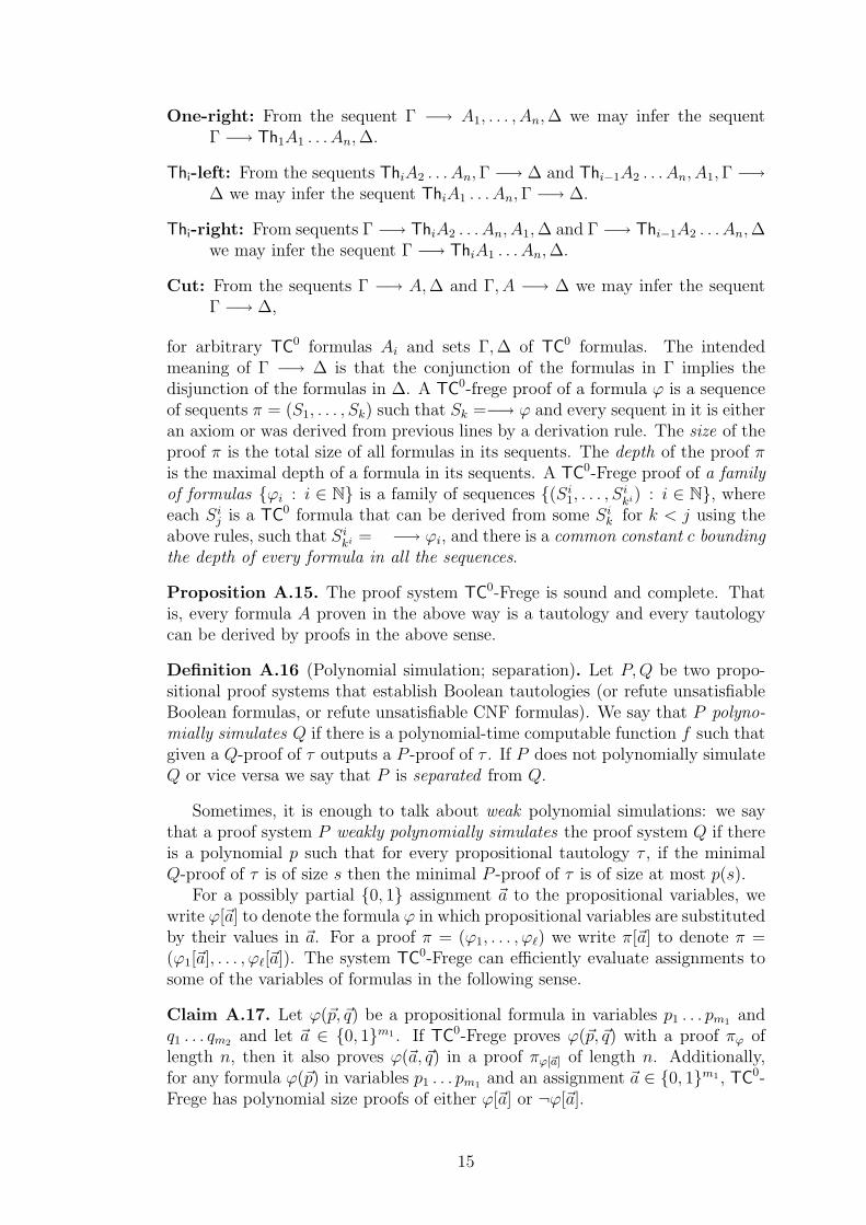
One-right: From the sequent Γ −→ A1, . . . , An,∆ we may infer the sequentΓ −→ Th1A1 . . . An,∆.

Thi-left: From the sequents ThiA2 . . . An,Γ −→ ∆ and Thi−1A2 . . . An, A1,Γ −→∆ we may infer the sequent ThiA1 . . . An,Γ −→ ∆.

Thi-right: From sequents Γ −→ ThiA2 . . . An, A1,∆ and Γ −→ Thi−1A2 . . . An,∆we may infer the sequent Γ −→ ThiA1 . . . An,∆.

Cut: From the sequents Γ −→ A,∆ and Γ, A −→ ∆ we may infer the sequentΓ −→ ∆,

for arbitrary TC0 formulas Ai and sets Γ,∆ of TC0 formulas. The intendedmeaning of Γ −→ ∆ is that the conjunction of the formulas in Γ implies thedisjunction of the formulas in ∆. A TC0-frege proof of a formula ϕ is a sequenceof sequents π = (S1, . . . , Sk) such that Sk =−→ ϕ and every sequent in it is eitheran axiom or was derived from previous lines by a derivation rule. The size of theproof π is the total size of all formulas in its sequents. The depth of the proof πis the maximal depth of a formula in its sequents. A TC0-Frege proof of a familyof formulas ϕi : i ∈ N is a family of sequences (Si

1, . . . , Siki) : i ∈ N, where

each Sij is a TC0 formula that can be derived from some Si

k for k < j using theabove rules, such that Si

ki = −→ ϕi, and there is a common constant c boundingthe depth of every formula in all the sequences.

Proposition A.15. The proof system TC0-Frege is sound and complete. Thatis, every formula A proven in the above way is a tautology and every tautologycan be derived by proofs in the above sense.

Definition A.16 (Polynomial simulation; separation). Let P,Q be two propo-sitional proof systems that establish Boolean tautologies (or refute unsatisfiableBoolean formulas, or refute unsatisfiable CNF formulas). We say that P polyno-mially simulates Q if there is a polynomial-time computable function f such thatgiven a Q-proof of τ outputs a P -proof of τ . If P does not polynomially simulateQ or vice versa we say that P is separated from Q.

Sometimes, it is enough to talk about weak polynomial simulations: we saythat a proof system P weakly polynomially simulates the proof system Q if thereis a polynomial p such that for every propositional tautology τ , if the minimalQ-proof of τ is of size s then the minimal P -proof of τ is of size at most p(s).

For a possibly partial 0, 1 assignment ~a to the propositional variables, wewrite ϕ[~a] to denote the formula ϕ in which propositional variables are substitutedby their values in ~a. For a proof π = (ϕ1, . . . , ϕℓ) we write π[~a] to denote π =(ϕ1[~a], . . . , ϕℓ[~a]). The system TC0-Frege can efficiently evaluate assignments tosome of the variables of formulas in the following sense.

Claim A.17. Let ϕ(~p, ~q) be a propositional formula in variables p1 . . . pm1 andq1 . . . qm2 and let ~a ∈ 0, 1m1 . If TC0-Frege proves ϕ(~p, ~q) with a proof πϕ oflength n, then it also proves ϕ(~a, ~q) in a proof πϕ[~a] of length n. Additionally,for any formula ϕ(~p) in variables p1 . . . pm1 and an assignment ~a ∈ 0, 1m1 , TC0-Frege has polynomial size proofs of either ϕ[~a] or ¬ϕ[~a].

15

Proof sketch: Consider with πϕ and substitute each occurrence of pi by ai. Theresulting proof remains correct and proves ϕ(~a, ~q), because every TC0-Frege ruleapplication is still correct after the assignment.

The second claim is proved by induction over the complexity of ϕ. If ϕ[~a]is true we can construct a proof by proving the (substitution instances of the)atomic formulas and then proceeding using the appropriate rules of the calculusby the way the formula is built up.

If ϕ[~a] is false, then we proceed in the same way as above with ¬ϕ[~a] insteadof ϕ[~a]. Claim

A.2 Theories of Bounded Arithmetic

In this section we give some of the necessary background from logic. Specifically,we present the theory V0 and its extension VTC0, as developed by Cook andNguyen [29] (see also [92]). These are weak systems of arithmetic, namely, frag-ments of Peano Arithmetic, usually referred to as theories of Bounded Arithmetic(for other treatments of theories of bounded arithmetic see also [20, 49, 57]). Thetheories are (first-order) two-sorted theories, having a first sort for natural num-bers and a second sort for finite sets of numbers (representing bit-strings via theircharacteristic functions). The theory V0 corresponds (in a manner made precise)to bounded depth Frege, and VTC0 corresponds to TC0-Frege (see Section A.2.2).The complexity classes AC0, TC0, and their corresponding function classes FAC0

and FTC0 are also defined using the two-sorted universe (specifically, the first-ordered sort [numbers] are given to the machines in unary representation and thesecond-sort as binary strings).

Definition A.18 (Language of two-sorted arithmetic L2A). The language of two-

sorted arithmetic, denoted L2A, consists of the following relation, function and

constant symbols:+, ·,≤, 0, 1, | |,=1,=2,∈ .

We describe the intended meaning of the symbols by considering the standardmodel N2 of two-sorted Peano Arithmetic. It consists of a first-sort universeU1 = N and a second-sort universe U2 of all finite subsets of N. The constants0 and 1 are interpreted in N2 as the appropriate natural numbers zero and one,respectively. The functions + and · are the usual addition and multiplication onthe universe of natural numbers, respectively. The relation ≤ is the appropriate“less or equal than” relation on the first-sort universe. The function |·| maps afinite set of numbers to its largest element plus one. The relation =1 is interpretedas equality between numbers, =2 is interpreted as equality between finite sets ofnumbers. The relation n ∈ N holds for a number n and a finite set of numbersN if and only if n is an element of N .

We denote the first-sort (number) variables by lower-case letters x, y, z, ...,and the second-sort (string) variables by capital letters X,Y, Z, .... We buildformulas in the usual way, using two sorts of quantifiers: number quantifiers andstring quantifiers. A number quantifier is said to be bounded if it is of the form∃x(x ≤ t ∧ . . . ) or ∀x(x ≤ t → . . . ), respectively, for some number term t thatdoes not contain x. We abbreviate ∃x(x ≤ t ∧ . . . ) and ∀x(x ≤ t → . . . ) by

16

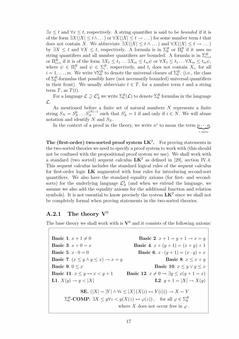
∃x ≤ t and ∀x ≤ t, respectively. A string quantifier is said to be bounded if it isof the form ∃X(|X| ≤ t∧ . . . ) or ∀X(|X| ≤ t→ . . . ) for some number term t thatdoes not contain X. We abbreviate ∃X(|X| ≤ t ∧ . . . ) and ∀X(|X| ≤ t → . . . )by ∃X ≤ t and ∀X ≤ t, respectively. A formula is in ΣB

0 or ΠB0 if it uses no

string quantifiers and all number quantifiers are bounded. A formula is in ΣBi+1

or ΠBi+1 if it is of the form ∃X1 ≤ t1 . . . ∃Xm ≤ tmψ or ∀X1 ≤ t1 . . . ∀Xm ≤ tmψ,

where ψ ∈ ΠBi and ψ ∈ ΣB

i , respectively, and ti does not contain Xi, for alli = 1, . . . ,m. We write ∀ΣB

0 to denote the universal closure of ΣB0 . (i.e., the class

of ΣB0 -formulas that possibly have (not necessarily bounded) universal quantifiers

in their front). We usually abbreviate t ∈ T , for a number term t and a stringterm T , as T (t).

For a language L ⊇ L2A we write ΣB

0 (L) to denote ΣB0 formulas in the language

L.As mentioned before a finite set of natural numbers N represents a finite

string SN = S0N . . . S

|N |−1N such that Si

N = 1 if and only if i ∈ N . We will abusenotation and identify N and SN .

In the context of a proof in the theory, we write nc to mean the term n · · ·n︸ ︷︷ ︸c times

.

The (first-order) two-sorted proof system LK2. For proving statements inthe two-sorted theories we need to specify a proof system to work with (this shouldnot be confused with the propositional proof system we use). We shall work witha standard (two sorted) sequent calculus LK2 as defined in [29], section IV.4.This sequent calculus includes the standard logical rules of the sequent calculusfor first-order logic LK augmented with four rules for introducing second-sortquantifiers. We also have the standard equality axioms (for first- and second-sorts) for the underlying language L2

A (and when we extend the language, weassume we also add the equality axioms for the additional function and relationsymbols). It is not essential to know precisely the system LK2 since we shall notbe completely formal when proving statements in the two-sorted theories.

A.2.1 The theory V0

The base theory we shall work with is V0 and it consists of the following axioms:

Basic 1. x+ 1 6= 0 Basic 2. x+ 1 = y + 1→ x = y

Basic 3. x+ 0 = x Basic 4. x+ (y + 1) = (x+ y) + 1

Basic 5. x · 0 = 0 Basic 6. x · (y + 1) = (x · y) + x

Basic 7. (x ≤ y ∧ y ≤ x)→ x = y Basic 8. x ≤ x+ y

Basic 9. 0 ≤ x Basic 10. x ≤ y ∨ y ≤ x

Basic 11. x ≤ y ↔ x < y + 1 Basic 12. x 6= 0→ ∃y ≤ x(y + 1 = x)

L1. X(y)→ y < |X| L2. y + 1 = |X| → X(y)

SE. (|X| = |Y | ∧ ∀i ≤ |X| (X(i)↔ Y (i)))→ X = Y

ΣB0 -COMP. ∃X ≤ y∀z < y(X(z)↔ ϕ(z)) , for all ϕ ∈ ΣB

0

where X does not occur free in ϕ .

17

Here, the Axioms Basic 1 through Basic 12 are the usual axioms used to definePeano Arithmetic without induction (PA−), which settle the basic properties ofaddition, multiplication, ordering, and of the constants 0 and 1. The Axiom L1says that the length of a string coding a finite set is an upper bound to the sizeof its elements. L2 says that |X| gives the largest element of X plus 1. SE is theextensionality axiom for strings which states that two strings are equal if theycode the same sets. Finally, ΣB

0 -COMP is the comprehension axiom scheme forΣB

0 formulas (it is an axiom for each such formula) and implies the existence ofall sets which contain exactly the elements that fulfill any given ΣB

0 property.When speaking about theories we will always assume that the theories are

two-sorted theories.

Proposition A.19 (Corollary V.1.8. [29]). The theory V0 proves the (number)induction axiom scheme for ΣB

0 formulas Φ:

(Φ(0) ∧ ∀x (Φ(x)→ Φ(x+ 1)))→ ∀zΦ(z).

In the above induction axiom, x is a number variable and Φ can have addi-tional free variables of both sorts.

The following is a basic notion needed to extend our language with new func-tion symbols (we write ∃!yΦ to denote ∃x(Φ(x)∧ ∀y(Φ(y/x)→ x = y)), where yis a new variable not appearing in Φ):

Definition A.20 (Two-sorted definability). Let T be a theory over the languageL ⊇ L2

A and let Φ be a set of formulas in the language L. A number function

f is Φ-definable in a theory T iff there is a formula ϕ(~x, y, ~X) in Φ such that Tproves

∀~x∀ ~X∃!yϕ(~x, y, ~X)

and it holds that2

y = f(~x, ~X)↔ ϕ(~x, y, ~X). (A.5)

A string function F is Φ-definable in a theory T iff there is a formula ϕ(~x, ~X, Y )in Φ such that T proves

∀~x∀ ~X∃!Y ϕ(~x, ~X, Y )

and it holds thatY = F (~x, ~X)↔ ϕ(~x, ~X, Y ). (A.6)

Finally, a relation R(~x, ~X) is Φ-definable in a theory T iff there is a formula

ϕ(~x, ~X, Y ) in Φ such that it holds that

R(~x, ~X)↔ ϕ(~x, ~X). (A.7)

The formulas (A.5), (A.6), and (A.7) are the defining axioms for f , F , and R,respectively.

Definition A.21 (Conservative extension of a theory). Let T be a theory in thelanguage L. We say that a theory T ′ ⊇ T in the language L′ ⊇ L is conservativeover T if every L formula provable in T ′ is also provable in T .

2Meaning it holds in the standard two-sorted model N2.

18

We can expand the language L and a theory T over the language L by addingsymbols for arbitrary functions f (or relations R) to L and their defining axiomsAf (or AR) to the theory T . If the appropriate functions are definable in T (ac-cording to Definition A.20) then the theory T +Af (+AR) is conservative over T .This enables one to add new function and relation symbols to the language whileproving statement inside a theory; as long as these function and relation symbolsare definable in the theory, every statement in the original language proved inthe extended theory (with the additional defining-axioms for the functions andrelations) is provable in the original theory over the original language. However,extending the language and the theory in such a way does not guarantee that onecan use the new function symbols in the comprehension (and induction) axiomschemes. In other words, using the comprehension (and induction) axioms overthe expanded language might not result in a conservative extension. Therefore,definability will not be enough for our purposes. We will show precisely in thesequel (Sections A.2.1 and A.2.2) how to make sure that a function is both de-finable in the theories we work with and also can be used in the correspondingcomprehension and induction axiom schemes (while preserving conservativity).

When expanding the language with new function symbols we can assume thatin bounded formulas the bounding terms possibly use function symbols from thethe expanded language.3

Extending V0 with new function and relation symbols

Here we describe a process (presented in Section V.4. in [29]) by which we canextend the language L2

A of V0 by new function symbols, obtaining a conservativeextension of V0 that can also prove the comprehension and induction axiomschemes in the extended language.

First note that every relation or function symbol has an intended or standardinterpretation over the standard model N2 (for instance, the standard interpreta-tion of the binary function “+” is that of the addition of two natural numbers).If not explicitly defined otherwise, we will always assume that a defining axiomof a symbol in the language defines a symbol in a way that its interpretation inN2 is the standard one. Note also that we shall use the same symbol F (~x, ~X)to denote a function and the function symbol in the (extended) language in thetheory.

Definition A.22 (Relation representable in a language). Let Φ be a set of formu-

las in a language L extending L2A. We say a relation R(~x, ~X) is representable by

a formula from Φ iff there is a formula ϕ(~x, ~X, Y ) in Φ such that in the standardtwo-sorted model N2 (and when all relation and function symbols in L get theirintended interpretation), it holds that:

R(~x, ~X)↔ ϕ(~x, ~X). (A.8)

We say that a number function f(~x, ~X) is polynomially-bounded if f(~x, ~X) ≤poly(~x, ~|X|). We say that a string function F (~x, ~X) is polynomially-bounded if

|F (~x, ~X)| ≤ poly(~x, ~|X|).3Because any definable function in a bounded theory can be bounded by a term in the

original language L2

A (cf. [29]).

19

Definition A.23 (Bit-definition). Let F (~x, ~X) be a polynomially-bounded string

function. We define the bit-graph of F to be the relation R(i, ~x, ~X), where i is anumber variable, such that

F (~x, ~X)(i)↔ i < t(~x, ~X) ∧R(i, ~x, ~X),

for some number term t(~x, ~X).

Definition A.24 (ΣB0 -definability from a language; Definition V.4.1.2. in [29]).

We say that a number function f is ΣB0 -definable from a language L ⊇ L2

A, iff is polynomially-bounded and its graph is represented by a ΣB

0 (L) formula ϕ.We call the formula ϕ the defining axiom of f . We say that a string functionF is ΣB

0 -definable from a language L ⊇ L2A, if F is polynomially-bounded and

its bit-graph is representable by a ΣB0 (L) formula ϕ. We call the formula ϕ the

defining axiom of F or the bit-defining axiom of F .

Note: We used the term defining axiom of a function f in both the case wheref is defined from a language (Definition A.24) and in case f is definable in thetheory (Definition A.20). We will show in the sequel that for our purposes thesetwo notions coincide: when we define a function from a language the functionwill be definable also in the relevant theory, and so the defining axiom of f fromthe language will be the defining axiom of f in the theory (when the theory ispossibly extended conservatively to include new function symbols).

Also, note that if the graph of a function F is representable by a ΣB0 (L)

formula then clearly also the bit-graph of F is representable by a ΣB0 (L) formula.

Therefore, it suffices to show a ΣB0 (L) formula representing the graph of a function

F to establish that F is ΣB0 -definable from L.

Definition A.25 (AC0-reduction). A number function f is AC0-reducible toL ⊇ L2

A iff there is a possibly empty sequence of functions F1, . . . , Fk such thatFi is ΣB

0 -definable from L ∪ F1, . . . , Fi−1, for any i = 1, . . . , k, and f is ΣB0 -

definable from L ∪ F1, . . . , Fk.We now describe the standard process enabling one to extend a theory T ⊇ V0

over the language L2A with new function symbols obtaining a conservative exten-

sion of T such that the new function symbols can also be used in comprehensionand induction axiom schemes in the theory (see Section V.4. in [29] for theproofs):

(i) If the number function f is ΣB0 -definable from L2

A, then T over the languageL2

A ∪f, augmented with the defining axiom of f , is a conservative exten-sion of T and we can also prove the comprehension and induction axiomsfor ΣB

0 (f) formulas.

(ii) If the string function F is ΣB0 -definable from L2

A, then T over the languageL2

A ∪ F, augmented with the bit-defining axiom of F , is a conservativeextension of T and we can also prove the comprehension and inductionaxioms for ΣB

0 (F ) formulas.

(iii) We can now iterate the above process of extending the language L2A(f) (or

equivalently, L2A(F )) to conservatively add more functions f2, f3, . . . to the

language, which can also be used in comprehension and induction axioms.

20

By the aforementioned and by Definition A.25, we can extend the language ofa theory with a new function symbol f , whenever f is AC0-reducible to L2

A. Thisresults in an extended theory (in an extended language) which is conservative, andcan prove the comprehension and induction axioms for formulas in the extendedlanguage. In the sequel, when defining a new function in V0 we may simplysay that it is ΣB

0 -definable (or bit-definable) in V0 and give its ΣB0 -defining (bit-

defining, respectively) axiom (that can possibly use also previously ΣB0 -defined

(or bit defined) function symbols).Extending the language of V0 with new relation symbols is simple: every

relation R(~x, ~X) which is representable by a ΣB0 (L) formula, where L is an ex-

tension of the language with new function symbols obtained as shown above, canbe added itself to the language. This results in a conservative extension of V0

that also proves the ΣB0 induction and comprehension axioms in the extended

language.

Definition A.26 (FAC0). A string (number) function is in FAC0 if it is poly-nomially bounded and its bit-graph (graph, respectively) is definable by a ΣB

0

formula in the language L2A.

Basic formalizations in V0

In this section we show how to formalize basic notions in the theory V0.

Characteristic function of a relation. For a given predicate R we denoteby χR the characteristic function of R. If R is ΣB

0 -definable in V0 then χR isΣB

0 -definable in V0, using the following defining axiom:

y = χR(~x, ~X)↔(R(~x, ~X)→ y = 1 ∧ ¬R(~x, ~X)→ y = 0

).

Natural number sequences of constant length. For two numbers x, y let〈x, y〉 := (x + y)(x + y + 1) + 2y be the pairing function, and let left(z), right(z)be the (easily ΣB

0 -definable in V0) projection functions of the first and secondelement in the pair z, respectively. It should be clear from the context when wemean 〈a, b〉 as an inner product of two vectors and when we mean it as the pairingfunction. We also ΣB

0 -define inductively 〈v1, . . . , vk〉 := 〈〈v1, . . . , vk−1〉, vk〉, forany constant k. Then V0 proves the injectivity of the pairing function and letsus handle such pairs in a standard way.

Notation: Given a number x, coding a sequence of natural numbers of lengthk, we write 〈x〉ki , for i = 1, . . . , k, to denote the number in the ith position in x.This is a ΣB

0 -definable function in V0 (defined via left(x), right(x) functions).

Rational numbers. Given the natural numbers, we can define the integers inV0 by identifying an integer number with a pair 〈a, b〉, such that a is its “positive”part and b is its “negative” part. We can define addition, product and subtractionof integers. All with ΣB

0 definitions.Having the integer numbers, we define the rational numbers as follows: for two

integer numbers a, b, the rational number a/b, is defined by the pair 〈a, b〉. Wecan define addition, subtraction and multiplication of rational numbers in V0 by

21

ΣB0 definitions. (See for example in [69]). However, we shall take a simpler path in

this paper: throughout this paper, all rational numbers used inside the

theories have the same denominator n2c, for some fixed constant c.This enables us to represent every rational number with a pair of integer numbers,such that each has a value polynomial in n. Addition and multiplication of tworational numbers is also ΣB

0 -definable in V0. This also makes it more convenientto sum a non-constant number of rational numbers in VTC0 (see PropositionA.33). To keep the invariant that all denominators are n2c, we then make surethat all the rational numbers resulting from computation in the proof in thetheory are indeed integer products of 1/n2c. This will hold since by inspection ofthe computations made in the theory it will be clear that:

1. all initial rational numbers will be integer products of 1/nc;

2. all arithmetic operations done on rational numbers are one of the following:

(a) addition of two rational numbers (this preserves the denominator);

(b) if we multiply two rational numbers x, y then x = nc·an2c and y = nc·b

n2c forsome two integers a, b, and so x·y = ab

n2c will have n2c as a denominator.

Convention: For the sake of readability we sometimes treat an integer numberm in the theory as its corresponding rational number m/1, thus enabling one tocompute with both types. (This is easy to achieve formally. E.g., one can definea function numones ′(X) that outputs the corresponding rational number of theinteger numones(X).)

Absolute numbers. We can ΣB0 -define in V0 the absolute value function for

integer numbers absZ(·) from the language L2A as follows (the function max is

easily ΣB0 -definable):

y = absZ(x) ↔ y = 〈max(left(x)− right(x), right(x)− left(x)), 0〉.

We ΣB0 -define the absolute value function for rational numbers absQ(·) in V0 as

follows:y = absQ(x) ↔ y = 〈absZ(left(x)), 〈n2c, 0〉〉.

For simplicity, we shall suppress the subscript Z,Q in absZ, absQ; the choiceof function can be determined from the context.

Number (natural, integers and rational) sequences of polynomial length.If we wish to talk about sequences of numbers (whether natural, integers or ratio-nals) where the lengths of the sequences are non-constant, we have to use stringvariables. Using the number tupling function we can encode sequences as sets ofnumbers (recall that a string is identified with the finite set of numbers encodingit). Essentially, a sequence is encoded as a string Z such that the xth numberin the sequence is y if the number 〈x, y〉 is in Z. Formally we have the followingΣB

0 -defining formula for the function seq(x, Z):

y = seq(x, Z)↔ (y < |Z| ∧ Z(〈x, y〉) ∧ ∀z < y¬Z(〈x, z〉))∨ (∀z < |Z|¬Z(〈x, z〉) ∧ y = |Z|). (A.9)

22

Formula (A.9) states that the xth element in the sequence coded by Z is y iff〈x, y〉 is in Z and no other number smaller than y also “occupies the xth positionin the sequence”, and that if no number occupies position x then the functionreturns the length of the string variable Z. We write Z[x] to abbreviate seq(x, Z).

According to the definition of the function seq(x, Z) above, there might bemore than one string Z that encodes the same sequence of numbers. However,we sometimes need to determine a unique string encoding a sequence. To thisend we use a ΣB

0 formula, denoted SEQ(y, Z), which asserts that Z is the lexi-cographically smallest string that encodes a sequence of y + 1 numbers (i.e., nostring with smaller binary code encodes the same sequence). Specifically, theformula states that if w = 〈i, j〉 is in Z then j is indeed the ith element in thesequence coded by Z, and for all y ≥ j the pair 〈i, y〉 is not contained in Z:

SEQ(y, Z) ≡∀w < |Z| (Z(w)↔ ∃i ≤ y∃j < |Z| (w = 〈i, j〉 ∧ j = Z[i])) .(A.10)

Note that elements of sequences Z coded by strings are referred to as Z[i], whileelements of sequences x coded by a number are referred to as 〈x〉ki (for k thelength of the sequence x). We define the number function length(Z) to be thelength of the sequence Z, as follows:

ℓ = length(Z)↔ SEQ(ℓ, Z) ∧ ∃w < |Z|∃j < |Z|(Z(w) ∧ w = 〈ℓ− 1, j〉) .

The defining axiom of length(Z) states that Z encodes a sequence and is thelexicographically smallest string that encodes this sequence and that the largestposition in the sequence which is occupied is ℓ− 1 (by definition there will be nopair 〈a, b〉 ∈ Z with a > ℓ− 1).

Array of strings. We want to encode a sequence of strings as an array. Weuse the relation RowArray(x, Z) to denote the xth string in Z as follows (wefollow the treatment in [29], Definition V.4.26, page 114).

Definition A.27 (Array of strings). The functionRowArray(x, Z), denoted Z [x],is ΣB

0 -definable in V0 using the following bit-definition:4

RowArray(x, Z)(i) ↔ (i < |Z| ∧ Z(〈x, i〉)).

We will abuse notation and write length(Z) for the length of the array Z(i.e., numbers of strings in Z) even when Z is a RowArray (and not a sequenceaccording to the predicate SEQ).

Functions for constructing sequences.

Definition A.28 (Sequencef (y, ~x, ~X)). Let f(z, ~x, ~X) be a ΣB0 -definable number

function in V0 (or a ΣB1 -definable number function in VTC0[see section A.2.2

below]), then Sequencef (y, ~x, ~X) is the string function ΣB0 -definable in V0(or ΣB

1 -

definable in VTC0, respectively) that returns the number sequence whose jth

position is f(j, ~x, ~X), for j = 0, . . . , y.

4We use the name “RowArray” (instead of the name “Row” used in [29]).

23

In other words, Sequencef (y, ~x, ~X) returns the graph of the function f(z, ~x, ~X)

up to y (that is, the sequence 〈f(0, ~x, ~X), . . . , f(y, ~x, ~X)〉). The following is the

ΣB0 -definition of the Sequencef (y, ~x, ~X):

Y = Sequencef (y, ~x, ~X) ↔ SEQ(y, Y ) ∧ ∀z ≤ y (Y [i] = f(z, ~x, ~X)).

Sequences of numbers with higher-dimensions. For a constant k, let S bea k-dimensional sequence of rational numbers. We encode a sequence S as a stringvariable Z such that the 〈i1, . . . , ik〉th element in S is extracted by the function seq(defined above). Specifically, we have S[〈i1, . . . , ik〉] = y iff 〈〈i1, . . . , ik〉, y〉 ∈ Zand there is no z < y for which 〈〈i1, . . . , ik〉, z〉 ∈ Z. Accordingly, we writeZ[i1, . . . , ik] to abbreviate seq(〈i1, . . . , ik〉, Z).

Matrices. Given a rational n× n matrix M , we define it as a two-dimensionalsequence in the manner defined above; and refer to the number at row 1 ≤ i ≤ nand column 1 ≤ j ≤ n of M as M [i, j]. We can define the string function thatextracts the xth row of M , and the xth column of M , respectively, with ΣB

0

formulas as follows. First define f(M, i, x) := M [i, x], g(M, i, x) := M [x, i], forany i = 0, 1, . . . , n (for i = 0, the value of M [i, x] and M [x, i] does not matter; butthis value is still defined by definition of the function seq). Then use DefinitionA.28 to define:

Row(i,M) := Sequencef (i, n)

Column(i,M) := Sequenceg(i, n) .

A.2.2 The theory VTC0

It is known that V0 is incapable of proving basic counting statements. Specifically,it is known that the function that sums a sequence of numbers (of non-constantlength) is not provably total, namely, is not ΣB

1 -definable in V0. Therefore, ifa proof involves such computations we might not be able to perform it in V0.The theory VTC0 extends V0, and is meant to allow reasoning that involvescounting, and specifically to sum a non-constant sequence of numbers. The theoryVTC0 was introduced in [70]; we refer the reader to Section IX.3.2 [29] for a fulltreatment of this theory. The ΣB

0 theorems of VTC0 correspond to polynomial-size TC0-Frege propositional proofs, which will enable us to prove the main resultof this paper.

Definition A.29 (NUMONES). Let δNUM(y,X, Z) be the following ΣB0 formula:

δNUM(y,X, Z) := SEQ(y, Z) ∧ Z[0] = 0 ∧ ∀u < y((X(u)→ Z[u+ 1] = Z[u] + 1)

∧ (¬X(u)→ Z[u+ 1] = Z[u])).

(A.11)

Define NUMONES to be the following ΣB1 formula:

NUMONES := ∃Z ≤ 1 + 〈y, y〉δNUM(y,X, Z). (A.12)

24

Informally one can think of the sequence Z(X), which existence is guaranteedby NUMONES, as a sequence counting the number of ones in a string X, that is,the uth entry in Z(X) is the number of ones appearing in the string X up to theuth position.

Definition A.30 (VTC0). The theory VTC0 is the theory containing all axiomsof V0 and the axiom NUMONES.

Using NUMONES we can define the function numones(y,X) that, given y andX, returns the yth entry of Z(X) via the following ΣB

1 -defining axiom

numones(y,X) = z ↔ ∃Z ≤ 1 + 〈|X| , |X|〉 (δNUM(|X| , X, Z) ∧ Z[y] = z) .(A.13)

We shall use the following abbreviation:

numones(X) := numones(|X| − 1, X).

Next we show how to obtain the functions we will use in the theory VTC0 (thesewill include the function numones).

Extending VTC0 with new function and relation symbols

Similar to the case of V0, we would like to extend the language L2A of VTC0 with

new function and relation symbols, to obtain a conservative extension. Moreover,we require that the new function and relation symbols could be used in inductionand comprehension axioms (while preserving conservativity). We can do this,using results from Sections I.X.3.2 and I.X.3.3 in [29], as follows.

Definition A.31 (Number summation). For any number function f(z, ~x, ~X) de-

fine the number function sumf (y, ~x, ~X) by5

sumf (y, ~x, ~X) =

y∑

i=0

f(i, ~x, ~X) .

Recall that by Definition A.24, a string (number) function F is ΣB0 -definable

from L ⊇ L2A iff there is a ΣB

0 formula over the language L that bit-defines(defines, respectively) the function F (when all the functions and relation symbolsin L get their intended interpretation).

We can use the following facts to extend the language of VTC0 with newfunction symbols (proved in Section IX.3.2 in [29]): if f is a (number or string)function in FTC0 (see below), then there is a ΣB

1 formula ϕ that represents itsgraph, and the theory VTC0 extended with the defining axiom for f (using ϕ,as in Definition A.24) over the language L = L2

A∪f is a conservative extensionof VTC0. And by Theorem IX.3.7 in Section IX.3.2 [29], VTC0 can prove theinduction and comprehension axioms for any ΣB

0 (L) formula.Thus, to extend VTC0 with new function symbols, by the above it suffices

to show how to obtain FTC0 functions. For this we use the following equivalentcharacterizations of FTC0 (see Sections IX.3.2 and IX.3.3 in [29]):

5Note that this is a definition in the metatheory (or in other words the standard two-sortedmodel).

25

Proposition A.32 (Theorem IX.3.12, Proposition IX.3.1 in [29]). The followingstatements are equivalent:

1. The function f is ΣB1 -definable in VTC0, and is applicable inside compre-

hension and induction axiom schemes.

2. The function f is in FTC0.

3. The function f is obtained from FAC0 by number summation and AC0-reductions.

4. There exist a natural k and functions f1, . . . , fk = f such that for everyi = 1, . . . , k, the function fi is either definbale by a ΣB

0 formula in thelanguage L2

A ∪ f1, . . . , fi−1 or there exists h ∈ L2A ∪ f1, . . . , fi−1 such

that fi = sumh.

5. The function f is AC0-reducible to L2A ∪ numones.

Therefore, to obtain new FTC0 functions, and hence to extend conservativelythe language of VTC0 with function symbols that can also be used in compre-hension and induction axioms, we can define a function with a ΣB

0 formula ina language that contains sumf , for f in FAC0, and possibly contains also othersymbols already definable in V0. Then, we can iterate this process a finite num-ber of times, where now sumf is defined also for f being a function defined in aprevious iteration. Since a function is in FTC0 iff it is ΣB

1 -definable in VTC0,new functions obtained in this way, are said to be ΣB

1 -definable in VTC0.To extend the language of VTC0 with new relation symbols, we can simply

add new ΣB0 -definable relations, using possibly relation and function symbols

that where already added before to the language, and specifically the numonesfunction. Such relations can then be used in induction and comprehension axioms,and we shall say that they are ΣB

0 -definable relations in VTC0.

Summation in VTC0

Here we show how to express and prove basic equalities and inequalities in thetheory VTC0.

Summation over natural and rational number sequences. Given a se-quence X of natural numbers, we define the function that sums the numbers inX until the yth position by sumseq(y,X) which is equal to

∑yi=0 seq(i,X).

To sum sequences of rational numbers, on the other hand, we do the following.For our purposes it is sufficient to sum many small (that is, polynomially bound-ed) numbers (this is in contrast to additions of numbers encoded as strings).Recall that we assume that all rational numbers in the theory have the samedenominator n2c, for some global constant c, independent of n.

Proposition A.33. Let X be a sequence of rational numbers with denominatorn2c and let sumQ(z,X) be the number function that outputs

∑zi=0X[i]. Then,

the number function sumQ(z,X) is ΣB1 -definable in VTC0.

26

Proof. It suffices to show that there is a ΣB0 formula that defines the number func-

tion sumQ(z,X) using only number summation functions and FAC0 functions.The AC0 function seq(i,X) extracts the ith element (that is, rational num-

ber) from the sequence X (see Formula (A.9)). A rational number is a pair ofintegers, and hence is a pair of pairs. Thus, gp(i,X) := left(left(seq(i,X))) ex-tracts the positive part of the integer numerator of the ith rational number inX, and gn(i,X) := right(left(seq(i,X))) extracts the negative part of the integernumerator of the ith rational number in X. Note that both gp(i,X) and gn(i,X)are FAC0 functions. Therefore, sumgp(z,X) equals the sum of all the positiveparts in X, and sumgn(z,X) equals the function that sums of all the negativeparts of the numerators in X. We can now define sumQ(z,X) as follows:

w = sumQ(z,X)↔ w =⟨〈sumgp(z,X), sumgn(z,X)〉 ,

⟨n2c, 0

⟩⟩(A.14)

Note indeed that 〈〈sumgp(z,X), sumgn(z,X)〉 , 〈n2c, 0〉〉 is a pair of integers thatencodes the desired rational number (with denominator n2c).

Notation: As a corollary from Proposition A.33, we can abuse notation asfollows: for f(y, ~x, ~X) a number function mapping to the rationals we write

sumf (n, ~x, ~X) to denote the sum of rationals∑n

i=0 f(i, ~x, ~X), for some fixed ~x, ~Xand n. Abusing notation further, we can write in a formula in the theory simply∑n

i=0 f(i, ~x, ~X).

Expressing vectors and operations on vectors. Vectors over Q are definedas sequences of rational numbers (for simplicity we shall assume that the numberat the 0 position of a vector is 0). Given two rational vectors v,u of size n, theirinner prduct, denoted 〈v,u〉, is defined as follows (we identify here v,u withthe string variables encoding v,u): let f(y,v,u) be the FAC0 number functiondefined by f(y) := v[y] · u[y]. Then the inner product of v and u is defined by

innerprod(v,u) := sumQ

(length(v) + 1, Sequencef (length(v) + 1)

).

The function that adds two rational vectors is easily seen to be in FAC0 (useDefinition A.28 to construct a sequence, where each entry in the sequence is theaddition of the corresponding entries of the two vectors).

Expressing product of matrices and vectors. Let v be an n-dimensionalrational vector and let M be an n×n rational matrix. Assume that f(z,M,v) :=innerprod(Row(z,M),v). We ΣB

1 -define in VTC0 the product Mv as follows:

Matvecprod(M,v) := Sequencef (length(v) + 1,M,v) .

Notation: When reasoning in the theory VTC0 we sometimes abuse nota-tion and write v · u or 〈v,u〉 instead of innerprod(u,v), and Mv instead ofMatvecprod(M,v), and utMv instead of 〈u,Mv〉.

27

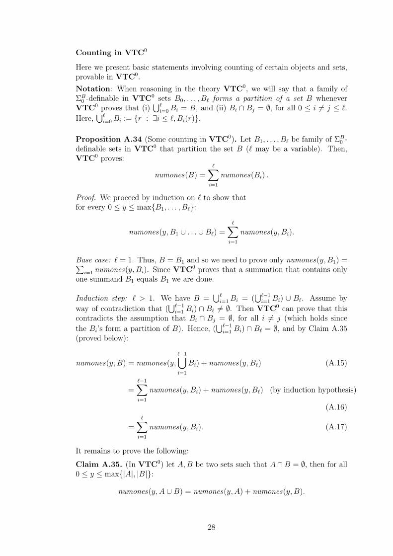
Counting in VTC0

Here we present basic statements involving counting of certain objects and sets,provable in VTC0.

Notation: When reasoning in the theory VTC0, we will say that a family ofΣB

0 -definable in VTC0 sets B0, . . . , Bℓ forms a partition of a set B wheneverVTC0 proves that (i)

⋃ℓi=0Bi = B, and (ii) Bi ∩ Bj = ∅, for all 0 ≤ i 6= j ≤ ℓ.

Here,⋃ℓ

i=0Bi := r : ∃i ≤ ℓ, Bi(r).

Proposition A.34 (Some counting in VTC0). Let B1, . . . , Bℓ be family of ΣB0 -

definable sets in VTC0 that partition the set B (ℓ may be a variable). Then,VTC0 proves:

numones(B) =ℓ∑

i=1

numones(Bi) .

Proof. We proceed by induction on ℓ to show thatfor every 0 ≤ y ≤ maxB1, . . . , Bℓ:

numones(y,B1 ∪ . . . ∪Bℓ) =ℓ∑

i=1

numones(y,Bi).

Base case: ℓ = 1. Thus, B = B1 and so we need to prove only numones(y,B1) =∑i=1 numones(y,Bi). Since VTC0 proves that a summation that contains only

one summand B1 equals B1 we are done.

Induction step: ℓ > 1. We have B =⋃ℓ

i=1Bi = (⋃ℓ−1

i=1 Bi) ∪ Bℓ. Assume by

way of contradiction that (⋃ℓ−1

i=1 Bi) ∩ Bℓ 6= ∅. Then VTC0 can prove that thiscontradicts the assumption that Bi ∩ Bj = ∅, for all i 6= j (which holds since

the Bi’s form a partition of B). Hence, (⋃ℓ−1

i=1 Bi) ∩ Bℓ = ∅, and by Claim A.35(proved below):

numones(y,B) = numones(y,ℓ−1⋃

i=1

Bi) + numones(y,Bℓ) (A.15)

=ℓ−1∑

i=1

numones(y,Bi) + numones(y,Bℓ) (by induction hypothesis)

(A.16)

=ℓ∑

i=1

numones(y,Bi). (A.17)

It remains to prove the following:

Claim A.35. (In VTC0) let A,B be two sets such that A ∩B = ∅, then for all0 ≤ y ≤ max|A|, |B|:

numones(y,A ∪B) = numones(y,A) + numones(y,B).

28

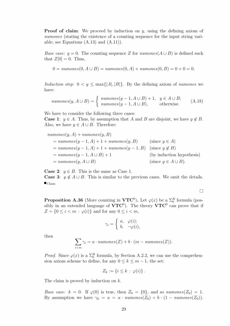
Proof of claim: We proceed by induction on y, using the defining axiom ofnumones (stating the existence of a counting sequence for the input string vari-able; see Equations (A.13) and (A.11)).

Base case: y = 0. The counting sequence Z for numones(A ∪B) is defined suchthat Z[0] = 0. Thus,

0 = numones(0, A ∪B) = numones(0, A) + numones(0, B) = 0 + 0 = 0.

Induction step: 0 < y ≤ max|A|, |B|. By the defining axiom of numones wehave:

numones(y,A ∪B) =

numones(y − 1, A ∪B) + 1, y ∈ A ∪B;numones(y − 1, A ∪B), otherwise.

(A.18)

We have to consider the following three cases:Case 1: y ∈ A. Thus, by assumption that A and B are disjoint, we have y 6∈ B.Also, we have y ∈ A ∪B. Therefore:

numones(y,A) + numones(y,B)

= numones(y − 1, A) + 1 + numones(y,B) (since y ∈ A)

= numones(y − 1, A) + 1 + numones(y − 1, B) (since y 6∈ B)

= numones(y − 1, A ∪B) + 1 (by induction hypothesis)

= numones(y,A ∪B) (since y ∈ A ∪B).

Case 2: y ∈ B. This is the same as Case 1.Case 3: y 6∈ A ∪ B. This is similar to the previous cases. We omit the details.

Claim

Proposition A.36 (More counting in VTC0). Let ϕ(x) be a ΣB0 formula (pos-

sibly in an extended language of VTC0). The theory VTC0 can prove that ifZ = 0 ≤ i < m : ϕ(i) and for any 0 ≤ i < m,

γi =

a, ϕ(i);b, ¬ϕ(i),

then ∑

i<m

γi = a · numones(Z) + b · (m− numones(Z)).

Proof. Since ϕ(x) is a ΣB0 formula, by Section A.2.2, we can use the comprehen-

sion axiom scheme to define, for any 0 ≤ k ≤ m− 1, the set:

Zk := i ≤ k : ϕ(i) .

The claim is proved by induction on k.

Base case: k = 0. If ϕ(0) is true, then Z0 = 0, and so numones(Z0) = 1.By assumption we have γ0 = a = a · numones(Z0) + b · (1 − numones(Z0)).

29

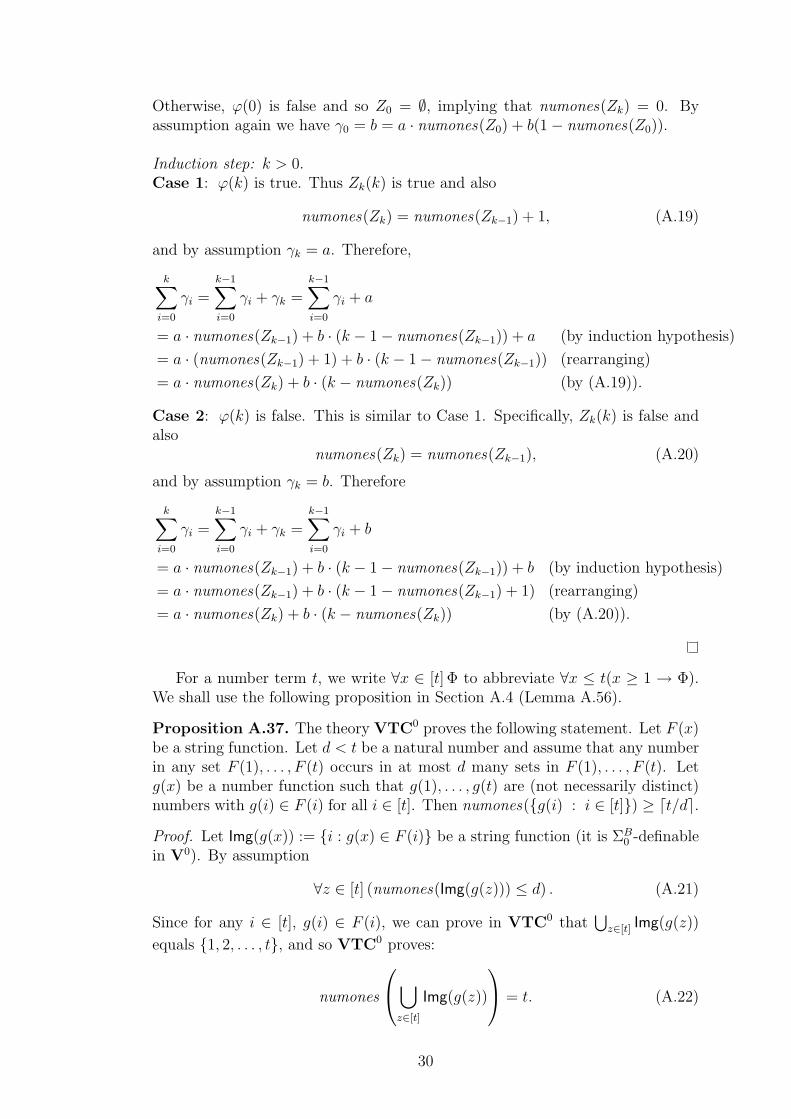
Otherwise, ϕ(0) is false and so Z0 = ∅, implying that numones(Zk) = 0. Byassumption again we have γ0 = b = a · numones(Z0) + b(1− numones(Z0)).

Induction step: k > 0.Case 1: ϕ(k) is true. Thus Zk(k) is true and also

numones(Zk) = numones(Zk−1) + 1, (A.19)

and by assumption γk = a. Therefore,

k∑

i=0

γi =k−1∑

i=0

γi + γk =k−1∑

i=0

γi + a

= a · numones(Zk−1) + b · (k − 1− numones(Zk−1)) + a (by induction hypothesis)

= a · (numones(Zk−1) + 1) + b · (k − 1− numones(Zk−1)) (rearranging)

= a · numones(Zk) + b · (k − numones(Zk)) (by (A.19)).

Case 2: ϕ(k) is false. This is similar to Case 1. Specifically, Zk(k) is false andalso

numones(Zk) = numones(Zk−1), (A.20)

and by assumption γk = b. Therefore

k∑

i=0

γi =k−1∑

i=0

γi + γk =k−1∑

i=0

γi + b

= a · numones(Zk−1) + b · (k − 1− numones(Zk−1)) + b (by induction hypothesis)

= a · numones(Zk−1) + b · (k − 1− numones(Zk−1) + 1) (rearranging)

= a · numones(Zk) + b · (k − numones(Zk)) (by (A.20)).

For a number term t, we write ∀x ∈ [t] Φ to abbreviate ∀x ≤ t(x ≥ 1 → Φ).We shall use the following proposition in Section A.4 (Lemma A.56).

Proposition A.37. The theory VTC0 proves the following statement. Let F (x)be a string function. Let d < t be a natural number and assume that any numberin any set F (1), . . . , F (t) occurs in at most d many sets in F (1), . . . , F (t). Letg(x) be a number function such that g(1), . . . , g(t) are (not necessarily distinct)numbers with g(i) ∈ F (i) for all i ∈ [t]. Then numones(g(i) : i ∈ [t]) ≥ ⌈t/d⌉.

Proof. Let Img(g(x)) := i : g(x) ∈ F (i) be a string function (it is ΣB0 -definable

in V0). By assumption

∀z ∈ [t] (numones(Img(g(z))) ≤ d) . (A.21)

Since for any i ∈ [t], g(i) ∈ F (i), we can prove in VTC0 that⋃

z∈[t] Img(g(z))

equals 1, 2, . . . , t, and so VTC0 proves:

numones

⋃

z∈[t]

Img(g(z))

= t. (A.22)

30

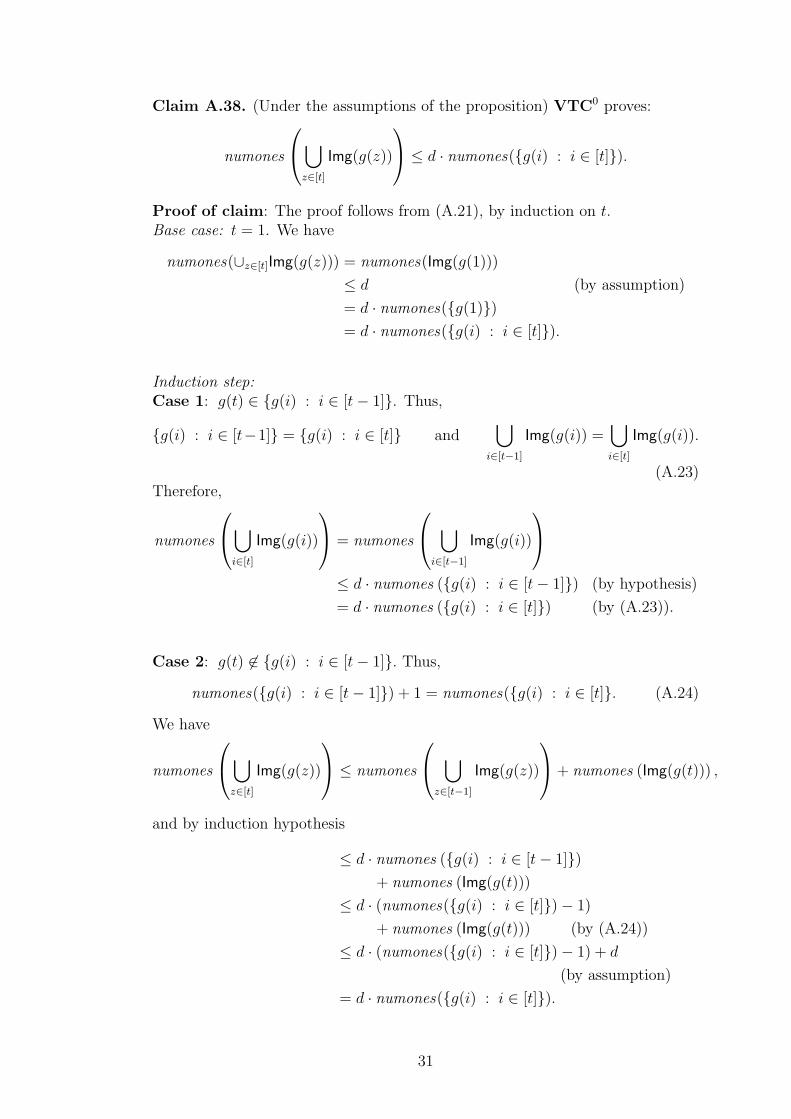
Claim A.38. (Under the assumptions of the proposition) VTC0 proves:

numones

⋃

z∈[t]

Img(g(z))

≤ d · numones(g(i) : i ∈ [t]).

Proof of claim: The proof follows from (A.21), by induction on t.Base case: t = 1. We have

numones(∪z∈[t]Img(g(z))) = numones(Img(g(1)))

≤ d (by assumption)

= d · numones(g(1))= d · numones(g(i) : i ∈ [t]).

Induction step:Case 1: g(t) ∈ g(i) : i ∈ [t− 1]. Thus,

g(i) : i ∈ [t−1] = g(i) : i ∈ [t] and⋃

i∈[t−1]

Img(g(i)) =⋃

i∈[t]

Img(g(i)).

(A.23)Therefore,

numones

⋃

i∈[t]

Img(g(i))

= numones

⋃

i∈[t−1]

Img(g(i))

≤ d · numones (g(i) : i ∈ [t− 1]) (by hypothesis)

= d · numones (g(i) : i ∈ [t]) (by (A.23)).

Case 2: g(t) 6∈ g(i) : i ∈ [t− 1]. Thus,

numones(g(i) : i ∈ [t− 1]) + 1 = numones(g(i) : i ∈ [t]. (A.24)

We have

numones

⋃

z∈[t]

Img(g(z))

≤ numones

⋃

z∈[t−1]

Img(g(z))

+ numones (Img(g(t))) ,

and by induction hypothesis

≤ d · numones (g(i) : i ∈ [t− 1])+ numones (Img(g(t)))

≤ d · (numones(g(i) : i ∈ [t])− 1)

+ numones (Img(g(t))) (by (A.24))

≤ d · (numones(g(i) : i ∈ [t])− 1) + d

(by assumption)

= d · numones(g(i) : i ∈ [t]).

31

Claim

Thus, by Claim A.38 and by (A.22), we get:

t ≤ d · numones(g(i) : i ∈ [t]),

which leads to t/d ≤ numones(g(i) : i ∈ [t]), and since numones(g(i) : i ∈[t]) is an integer number we get:

⌈t/d⌉ ≤ ⌈numones(g(i) : i ∈ [t])⌉ = numones(g(i) : i ∈ [t]).

Manipulating big sums in VTC0

We need to prove basic properties of summation (having a non-constant numberof summands) like commutativity, associativity, distributivity, substitution in bigsums, rearranging etc., in VTC0, to be able to carry out basic calculations in thetheory. As a consequence of this section we will be able to freely derive inequal-ities and equalities between big summations (using rearranging, substitutions ofequals, etc.) in VTC0.

Proposition A.39 (Basic properties of sums in VTC0). In what follows weconsider the theory VTC0 over an extended language (including possibly newΣB

1 -definable function symbols in VTC0 and their defining axioms). The functionf(i) is a number function symbol mapping to the rationals or naturals (possiblywith additional undisplayed parameters). The theory VTC0 proves the followingstatements:

Substitution: Assume that u(i), v(i) are two terms (possibly with additionalundisplayed parameters), such that u(i) = v(i) for any i ≤ n, then

n∑

i=0

f(u(i)) =n∑

i=0

f(v(i)).

Distributivity: Assume that u is a term that does not contain the variable i,then

u ·n∑

i=0

f(i) =n∑

i=0

u · f(i).

Rearranging: Assume that I = 0, . . . , n and let I1, . . . , Ik be a definable par-tition of I (specifically, the sets I1, . . . , Ik are all ΣB

0 -definable in VTC0 andVTC0 proves that the Ij’s form a partition of I). Then

n∑

i=0

f(i) =k∑

j=1

∑

i∈Ij

f(i),

where∑

i∈Ijf(i) denotes the term

∑|Ij |−1i=0 f(δ(i)) where δ(i) is the function

that enumerates (in ascending order) the elements in Ij.

32

Inequalities: Let g(i) be a number function mapping to the rationals or naturals(possibly with additional undisplayed parameters), such that f(i) ≤ g(i) forall 0 ≤ i ≤ n, then

n∑

i=0

f(i) ≤n∑

i=0

g(i).

Proof.Substitution: When we work in the theory VTC0 we implicitly assume thatwe have equality axioms stating that if t = t′, for any two terms t, t′, then F (t) =F (t′), for any function F (including functions F that are from the extendedlanguage of VTC0). Since we assume that f(i) is a ΣB

1 -definable number functionin VTC0, the function g(n) :=

∑ni=0 f(i) is also ΣB

1 -definable in VTC0, and sowe also have the equality axiom for g(n). Thus, if u(i) = v(i), for any i ≤ n, thenwe can prove also g(u(n)) = g(v(n)).

Distributivity: This is proved simply by induction on n. We omit the details.

Rearranging: Because I1, . . . , Ik are ΣB0 -definable sets in VTC0 we can define

the family of sequences S1, . . . , Sk, each of length n+ 1, such that

Sj[i] :=

f(i), i ∈ Ij ;0, otherwise.

The theory VTC0 proves, by induction on n, that

k∑

j=1

n∑

i=0

Sj[i] =n∑

i=0

f(i).

For any j = 1, . . . , k, we can ΣB1 -define in VTC0 the function δj : 0, . . . , |Ij| −

1 → 0, . . . , n such that δj(ℓ) = i iff i is the (ℓ+ 1)th element in Ij (when theelements in Ij are ordered in ascending order). In other words, the δj’s functionsenumerate the elements in Ij.

We can now prove in VTC0 that

n∑

i=0

Sj[i] =

|Ij |−1∑

i=0

f(δj(i)),

from which, by Substitution (proved above), we can prove:

k∑

i=1

n∑

i=0

Sj[i] =k∑

i=1

|Ij |−1∑

i=0

f(δj(i)).

Inequalities: This can be proved in VTC0 simply by induction on n. We omitthe details.

All the equalities and inequalities which contain big summations that we willderive in the theory, can be proved using Proposition A.39. We shall not statethis explicitly in the text, but continue to derive such equalities and inequalitiesfreely.

33

The relation between VTC0 and TC0-Frege

In this section we show how one can translate a ΣB0 formula ϕ into a family

of propositional formulas JϕK. We then state the theorem showing that if theuniversal closure of a ΣB

0 formula ϕ is provable in VTC0 then the propositionaltranslation JϕK has a polynomial-size proof in TC0-Frege.

Definition A.40 (Propositional translation J·K of ΣB0 formulas). Let ϕ(~x, ~X) be

a ΣB0 formula. The propositional translation of ϕ is a family

JϕK = JϕK~m;~n | mi, ni ∈ N

of propositional formulas in variables pXi

j for everyXi ∈ ~X. The intended meaningis that JϕK is a valid family of formulas if and only if the formula

∀~x∀ ~X((∧|Xi| = ni)→ ϕ(~m, ~X)

)

is true in the standard model N2 of two sorted arithmetic, where n denotes thenth numeral, for any n ∈ N.

For given ~m,~n ∈ N we define JϕK by induction on the size of the formulaJϕK~m;~n. We denote the value of a term t by val(t).

Case 1: Let ϕ(~x, ~X) be an atomic formula.

• If ϕ(~x, ~X) is ⊤ (or ⊥), then JϕK~m,~n := ⊤ (or ⊥).

• If ϕ(~x, ~X) is Xi = Xi, then JϕK~m,~n := ⊤.

• If ϕ(~x, ~X) is Xi = Xj for i 6= j, then (using the fact that V0contains theextensionality axiom SE) instead of translating ϕ, we translate the V0-equivalent formula

|Xi| = |Xj| ∧ ∀k ≤ |X| (Xi(k)↔ Xj(k))).

• If ϕ(~x, ~X) is t1(~y, |~Y |) = t2(~z, |~Z|) for terms t1, t2, number variables ~y, ~z and

string variables ~Y , ~Z, where ~y ∪ ~z = ~x and ~Y ∪ ~Z = ~X, and ~my, ~mz and~nY , ~nZ denote the corresponding assignments of numerals ~m,~n to the ~y, ~zand ~Y , ~Z variables, respectively. Then

JϕK~m,~n :=

⊤ if val(t1(~m

Y , ~nY )) = val(t2(~mZ , ~nZ)) and

⊥ otherwise.

• If ϕ(~x, ~X) is t1(~y, |~Y |) ≤ t2(~z, |~Z|) for terms t1, t2, number variables ~y, ~z and

string variables ~Y , ~Z, then

JϕK~m,~n :=

⊤ if val(t1(~m

Y , ~nY )) ≤ val(t2(~mZ , ~nZ)) and

⊥ otherwise.

34

• If ϕ(~x, ~X) is Xi(t(~x, | ~X|)), then

JϕK~m,~n := ⊥ if ni = 0

and otherwise

JϕK~m,~n :=

pXi

val(t(~m,~n)) if val(t(~m,~n)) < ni − 1,

⊤ if val(t(~m,~n)) = ni − 1,

⊥ if val(t(~m,~n)) > ni − 1.

Case 2: The formula ϕ is not atomic.

• If ϕ ≡ ψ1 ∧ ψ2 we let

JϕK~m,~n := Jψ1K~m,~n ∧ Jψ2K~m,~n.

• If ϕ ≡ ψ1 ∨ ψ2 we let

JϕK~m,~n := Jψ1K~m,~n ∨ Jψ2K~m,~n.

• If ϕ ≡ ¬ψ we letJϕK~m,~n := ¬JψK~m,~n.

• If ϕ ≡ ∃y ≤ t(~x, | ~X|)ψ(y, ~x, ~X) then

JϕK~m,~n :=

val(t(~m,~n))∨

i=0

Jψ(i, ~x, ~X)K~m,~n.

• If ϕ ≡ ∀y ≤ t(~x, | ~X|)ψ(y, ~x, ~X) then

JϕK~m,~n :=

val(t(~m,~n))∧

i=0

Jψ(i, ~x, ~X)K~m,~n.

This concludes the translation for ΣB0 formulas.

Proposition A.41 (Lemma VII.2.2 [29]). For every ΣB0 formula ϕ(~x, ~X) there

exists a constant d ∈ N and a polynomial p(~m,~n) such that for all ~m,~n ∈ N,

the propositional translation Jϕ(~x, ~X)K~m,~n has depth at most d and size at mostp(~m,~n).

We can now state the relation between provability of an arithmetical statementϕ in VTC0 to the provability of the family JϕK in TC0-Frege as follows.

Theorem A.42 (Section X.4.3. [29]). Let ϕ(~x, ~X) be a ΣB0 formula. Then, if

VTC0 proves ϕ(~x, ~X) then there is a polynomial size family of TC0-Frege proofsof JϕK.

35

A.3 Feige-Kim-Ofek Witnesses and the Main For-

mula

In this section we define the main formula we are going to prove in the theory. Weare concerned with proofs of 3CNF formulas. Let us fix the following notation.With n we will denote the number of propositional variables x1, . . . , xn and withm we will denote the number of clauses appearing in the 3CNF denoted C =∧m−1

α=0 Cα. Each clause Cα is of the form xℓ1i ∨ xℓ2

j ∨ xℓ3k , for ℓ1, ℓ2, ℓ3 ∈ 0, 1,

where x1i abbreviates xi and x0

i abbreviates ¬xi. A clause Cα is represented bythe sequence 〈i, j, k, 〈ℓ1, ℓ2, ℓ3〉, α〉. The defining ΣB

0 formula of the relation is:

Clause(x, n,m)↔ ∃i, j, k ≤ n∃α < m∃ℓ ≤ 8

(i > 0 ∧ j > 0 ∧ k > 0 ∧ 〈x〉51 = i ∧ 〈x〉52 = j ∧ 〈x〉53 = k ∧ 〈x〉54 = ℓ ∧ 〈x〉55 = α).

A 3CNF C ≡ ∧m−1α=0 Cα is represented by the sequence (C0, . . . , Cm−1). Since m

is non-constant, we use a string variable to code C. The defining ΣB0 formula of

this relation is

3CNF(C, n,m)↔ ∀i < m(Clause(C[i], n,m) ∧ 〈C[i]〉55 = i

).

For a number variable x, we ΣB0 -define Even(x) by the formula ∃y ≤ x(2 ·y =

x) (meaning that x is an even number). Accordingly, we define Odd(x) by¬even(x).

For some clause C and a string variable A (interpreted as a Boolean assign-ment), we ΣB

0 -define the following predicate, stating that C is not satisfied underthe assignment A:

NotSAT(C,A) ≡∃i, j, k ≤ n(〈C〉51 = i ∧ (A(i)↔ 〈〈C〉54〉31 = 0)

)

∧(〈C〉52 = j ∧ (A(j)↔ 〈〈C〉54〉32 = 0)

)

∧(〈C〉53 = k ∧ (A(k)↔ 〈〈C〉54〉33 = 0)

).

We need the following notations and definitions to facilitate the formalizationof certain sets and objects:

Notation:

1. When considering a set of clauses, then a clause in C will be referred toonly by its index 0 ≤ i < m. Thus, a set of clauses from C is a set ofnatural numbers less than m.

2. A set of literal positions from C will be coded as a set of numbers 〈a, b〉,where 0 ≤ a < m is the index of a clause in C and b = 1, 2, 3 is the indexof a literal in the clause.

3. For 0 ≤ i < m and ε = 0, 1 and a sequence S of 3-clauses we defineLitPos(S, i, ε) to be the string function that outputs the set of (positions of)literals xε

i in S. In other words, we have:

LitPos(S, i, ε) :=〈j, ℓ〉 : j < length(S) ∧ ℓ ≤ 3 ∧ 〈S[j]〉5ℓ = i ∧ 〈〈S[j]〉54〉3ℓ = ε

.

36

4. Let satLit(A,C) be the string function that outputs the set of all literalpositions in C that are satisfied by A.

5. The function Lit(C, i) returns the ith literal xεj of the clause C, for i = 1, 2, 3,

in the form of a pair 〈j, ε〉.

6. If the literals of a clause are not all true or not all false under A, then wesay that the clause is satisfied as NAE (standing for “not all equal”) by A.We can easily ΣB

0 -define the predicate SatL(z, A), stating that the literalz is satisfied by the assignment A in VTC0. Let:

NAE(C,A) ↔Clause(C) ∧∨

i=1,2,3

SatL (Lit(C, i), A)∧∨

i=1,2,3

¬SatL (Lit(C, i), A)

be the ΣB0 relation that states that the assignment A satisfies the 3-clause

C as NAE. Let satNAE(A,C) be the string function that outputs the set ofclauses in C that are satisfied as NAE by A.

The functions LitPos(S, i, ε), satLit(A,C) and satNAE(A,C) above are all AC0-reducible to the language L2

A and so we can assume that we have these functions(along with their defining axioms) in VTC0 (see Section A.2.1). All the functionsin this section will be AC0-reducible to L2

A ∪numones, and all the relations inthis section will have ΣB

0 definitions in the language L2A extended to include both

our new function symbols and numones .

Definition A.43 (Even k-tuple). For any given k, a sequence S of k clauses is aneven k-tuple iff every variable appears an even number of times in the sequence.Formally, the predicate is denoted TPL(S, k):

TPL(S, k) ↔ length(S) = k ∧∀i ≤ n, Even (numones(LitPos(S, i, 0)) + numones(LitPos(S, i, 1))) .

(A.25)

Observe that if S is an even k-tuple then k is even (since the total number ofvariable occurrences N is even, by assumption that each variable occurs an evennumber of times; and k = N/3, since each clause has three variables).

Definition A.44 (Inconsistent k-tuple). An even k-tuple is said to be inconsis-tent if the total number of negations in its clauses is odd. Formally, the predicateis denoted by ITPL(S, k):

ITPL(S, k)↔ TPL(S, k) ∧Odd

(n∑

i=1

numones(LitPos(S, i, 1))

).

Definition A.45 (The imbalance Imb(S, y)). For a 3CNF S we define the func-tion i-imbalance iImb(S, i) to be the absolute value of the difference of negat-ed occurrences of xi and non-negated occurrences of xi in the 3CNF S (where

37

x1, . . . , xn are considered to be all the variables in S). It is defined simply by theterm:

iImb(S, i) := abs(numones(LitPos(i, 0, S))− numones(LitPos(i, 1, S))).

For a 3CNF S, the predicate imbalance of S, denoted Imb(S, y), is true iff yequals the sum over the i-imbalances of all the variables, that is:

Imb(S, y)↔ y =n∑

i=1

iImb(S, i).

Definition A.46 ((t, k, d)-collection). A (t, k, d)-collection D of a 3CNF C withm clauses is an array (coded as in Definition A.27) of t many inconsistent k-tuples, which contain only clauses from C, and each clause appears in at mostd many such inconsistent k-tuples. The predicate is denoted Coll(t, k, d,C,D)and is defined by the following formula:

length(D) = t∧∀i < t ITPL(D [i], k)∧∀i < t∀ℓ < k∃j < |C| (D [i][ℓ] = C[j])∧

∀j < |C|t−1∑

i=0

k−1∑

ℓ=0

χ=(〈D [i][ℓ]〉55, j) ≤ d.

Definition A.47 (Mat(M,C)). We define the predicate Mat(M,C) that holdsiff M is an n × n rational matrix such that Mij equals 1

2times the number of

clauses in C where xi and xj appear with different polarity minus 12

times thenumber of clauses where they appear with the same polarity. More formally, wehave

Mij :=m−1∑

k=0

E(k)ij , for any i, j ∈ [n], (A.26)

where E(k)ij corresponds to the kth clause in C as follows:

E(k)ij :=

12, xεi

i , xεj

j ∈ C[k] and εi 6= εj, for some εi, εj ∈ 0, 1 and i 6= j;−1

2, xεi

i , xεj

j ∈ C[k] and εi = εj, for some εi, εj ∈ 0, 1 and i 6= j;0, otherwise.

(A.27)

Note that E(k)ij is definable by a ΣB

0 formula (in L2A), and so Mat(M,C) is a

ΣB0 -definable relation in VTC0.

Finally, we need a predicate EigValBound(M,~λ, V ) that ensures that ~λ isa collection of n rational approximations of the eigenvalues of the matrix M andthat V is the rational matrix whose rows are the rational approximations of theeigenvectors of M (where the ith row in V is the approximation of the approx-imate eigenvector λi). For the sake of readability we defer the formal definition

of the predicate EigValBound(M,~λ, V ) and all the lemmas that relate to it,including the proofs in the theory making use of this predicate, to Section A.5.

Notation: 1. The notation o(1) appearing inside a formula in the proof withinthe theory, and specifically in Definition A.48 below, stands for a term of the

38

form b/nc, for b a number symbol greater than 0, and c some positive constant(and where a rational number is encoded in the way described in Section A.2.1).

2. Given two terms t and f(n) in the language L2A, where n is a number

variable, we say that VTC0 proves t = O(f(n)), to mean that there exists someconstant c (independent of n) such that VTC0 proves t ≤ c · f(n), where c is aterm without variables in the language L2

A.

We can now state the main formula that we are going to prove in VTC0. Itsays that if the Feige-Kim-Ofek witness fulfills the inequality t > d·(I+λn)

2+ o(1)

then there exists a clause in C that is not satisfied by any assignment A (one canthink of all the free variables in the formula as universally quantified):

Definition A.48 (The main formula). The main formula is the following formula

(~λ denotes n distinct number parameters λ1, . . . , λn):

(3CNF(C, n,m) ∧Coll(t, k, d,C,D) ∧ Imb(C, I) ∧Mat(M,C)∧

EigValBound(M,~λ, V ) ∧ λ = maxλ1, . . . , λn ∧ t >d · (I + λn)

2+ o(1)

)

−→ ∃i < mNotSAT(C[i], A).

A.4 Proof of the Main Formula

In this section we prove our key theorem:

Theorem A.49 (Key). The theory VTC0 proves the main formula (DefinitionA.48).

Proof. We reason inside VTC0. Assume by way of contradiction that the premiseof the implication in the main formula holds and that there is an assignmentA ∈ 0, 1n (construed as a string variable of length n) that satisfies every clausein C. Recall that satLit(A,C) is the set of all literal positions that are satisfiedby A.

Lemma A.50. (Assuming the premise of the main formula) the theory VTC0

proves:

numones(satLit(A,C)) ≤ 3m+ I

2.

Proof. First observe that for any assignment A and any 1 ≤ i ≤ n the setof satisfied literals of xi is defined by LitPos(C, i, A(i)). Therefore, the setsLitPos(C, 1, A(1)), . . . , LitPos(C, n, A(n)) form a partition of satLit(A,C) (prov-ably in VTC0), and thus by Proposition A.34, VTC0 proves that

numones(satLit(A,C)) =n∑

i=1

numones(LitPos(C, i, A(i))). (A.28)

39

By (A.28) we get

numones(satLit(A,C)) ≤n∑

i=1

maxnumones(LitPos(C, i, 0)), numones(LitPos(C, i, 1)).

(A.29)For any 1 ≤ i ≤ n, define the term

LitPos(C, i) := LitPos(C, i, 0) ∪ LitPos(C, i, 1).

Then by

iImb(C, i) + numones(LitPos(C, i))

2=

iImb(C, i) + numones(LitPos(C, i, 0)) + numones(LitPos(C, i, 1))

2,

and since, by Definition A.45,iImb(C, i) = abs (numones(LitPos(C, i, 0))− numones(LitPos(C, i, 1))), the theo-ry VTC0 proves that for any 1 ≤ i ≤ n:

maxnumones(LitPos(C, i, 0)), numones(LitPos)(C, i, 1) =

iImb(C, i) + numones(LitPos(C, i))

2.

(A.30)

Claim A.51. (Assuming the premise of the main formula) the theory VTC0

proves:n∑

i=1

iImb(C, i) + numones(LitPos(C, i))

2=I + 3m

2.

Proof of claim: First recall the definition of imbalance (Definition A.45) I =∑ni=1 iImb(C, i). Thus it remains to prove that

∑ni=1 numones(LitPos(C, i)) =

3m. For this, note that LitPos(C, i), for i = 1, . . . , n, partition the set of allliteral positions in C. In other words, we can prove that: (i) if H is the set ofall literal positions in C (this set is clearly ΣB

0 -definable in VTC0) then H =∪n

i=1LitPos(C, i); and (ii) LitPos(C, i) ∩ LitPos(C, j) = ∅, for all 1 ≤ i 6= j ≤ n.Therefore, by Proposition A.34 we can prove that:

numones(H) =n∑

i=1

numones(LitPos(C, i)). (A.31)

Now, the set H of all literal position in C can be partitioned (provably in VTC0)by the sets T1, . . . , Tm, where each Tj, for 0 ≤ j < m, is the set of the threeliterals in the jth clause in C. Thus, again by Proposition A.34, we can provethat numones(H) = 3m. By (A.31) we therefore have

n∑

i=1

numones(LitPos(C, i)) = 3m.

Claim

40

We conclude that:

numones(satLit(A,C))

≤n∑

i=1

maxnumones(LitPos(C, i, 0)), numones(LitPos(C, i, 1)) (by (A.29))

=n∑

i=1

iImb(C, i) + LitPos(C, i)

2(by (A.30))

=I + 3m

2. (by Claim A.51).

We now bound the number of clauses in C that contain exactly two literalssatisfied by A. We say that a 3-clause is satisfied by a given assignment as NAE(which stands for not all equal) if the literals in the clause do not all have thesame truth values. That is, if either exactly one or exactly two literals in theclause are satisfied by the assignment.

Recall that satNAE(A,C) is the function that returns the set of all clauses(formally, indices < m) that are satisfied as NAE by A.

Lemma A.52. (Assuming the premise of the main formula) the theory VTC0

proves: let h be the number of clauses in C that contain exactly two literalssatisfied by A. Then

h ≤ 3m+ I

2− 3m+ 2 · numones(satNAE(A,C)) .

Proof. For i = 0, 1, 2, 3, let Bi be the set of clauses in C that contain exactly iliterals satisfied by A. For i = 0, 1, 2, 3, let Fi be the string function that mapsa clause (index) C to the set of literal positions that are satisfied by A in casethere are exactly i such literals and to the empty set otherwise:

Fi(j) =

l1, . . . , li, if j ∈ Bi ;∅, otherwise

(where a literals lk is coded, as before, by the pair 〈a, b〉 for a an index of a clausein C and b the position of the literal in the clause). Every such function Fi isΣB

0 -defined in VTC0. We also ΣB0 -define the image of Fi as follows:

Img(Fi) := x : ∃y < m (Fi(y))(x).

Claim A.53. (Assuming the premise of the main formula) the theory VTC0

proves:

numones(satLit(A,C)) =3∑

i=1

numones(Img(Fi)).

Proof of claim: In light of Proposition A.34, it suffices to prove that satLit(A,C)is partitioned by Img(F1), Img(F2), Img(F3) (note that Img(F0) = ∅ by defini-tion), in the sense that:

(i) satLit(A,C) = Img(F1) ∪ Img(F2) ∪ Img(F3), and

41

(ii) Img(Fi) ∩ Img(Fj) = ∅, for all 1 ≤ i 6= j ≤ 3.

We prove (i): consider a literal x ∈ satLit(A,C), and let x = 〈a, b〉. We knowthat the clause Ca contains the literal x. Now, either zero, or one, or two of theremaining literals in Ca are satisfied by A. So x must be in either F1(a) or inF2(a) or in F3(a), respectively. Item (ii) is easy to prove by the definition of theFi’s. We omit the details. Claim

Claim A.54. For any i = 1, 2, 3, numones(Img(Fi)) = i · numones(Bi).

Proof of claim: Fix some i = 1, 2, 3. We prove the claim by induction onthe number of clauses j < m (we can consider the sets Bi and the functionsFi having an additional parameter that determines until which clause to buildthe sets. That is, Bi(z) is the set of clauses from 0 to z that have i literalssatisfied by A; and similarly we add a parameter for the Fi’s). In the base casej = 0 there is only one clause C0. Depending on A we know how many literalsin C0 are satisfied by A. And so 0 ∈ Bi iff i literals are satisfied by A in C0 iffnumones(Fi(0)) = i = i · 1 = i · numones(Bi). The induction step is similar andwe omit the details. Claim

By Claim A.53 and Claim A.54 we get:

numones(satLit(A,C)) =∑

i=1,2,3

numones(Img(Fi))

=∑

i=1,2,3

i · numones(Bi) . (A.32)

It is easy to show (in a similar manner to Claim A.53) that B1 ∪ B2 ∪ B3 =0, . . . ,m − 1 and Bi ∩ Bj = ∅, for any 1 ≤ i 6= j ≤ 3. From this, usingProposition A.34, we get that m = numones(B1)+numones(B2)+numones(B3),and so:

numones(B1) = m− numones(B2)− numones(B3) . (A.33)

Thus, by (A.32):

numones(satLit(A,C)) = m− numones(B2)− numones(B3) (A.34)

+ 2 · numones(B2) + 3 · numones(B3)

= m+ 2 · numones(B3) + numones(B2) ,

and so

numones(B2) =numones(satLit(A,C))−m− 2 · numones(B3) . (A.35)

The set of clauses in C that are NAE satisfied by A (i.e., satNAE(A,C)) is equalto the set of clauses having either one or two literals satisfied by A; the lattertwo sets are just B1 and B2, and since they are (provably in VTC0) disjoint wehave (using also (A.33)):

numones(B3) = m−(numones(B1)+numones(B2)) = m−numones(satNAE(A,C)) .

42

Plugging this into (A.35), and using Lemma A.50, we get:

numones(B2) = numones(satLit(A,C))− 3m+ 2 · numones(satNAE(A,C))

≤ 3m+ I

2− 3m+ 2 · numones(satNAE(A,C)).

This concludes the proof of Lemma A.52

The following lemma provides an upper bound on the number of clauses in Cthat can be satisfied as NAE by the assignment A.

Lemma A.55. (Assuming the premise of the main formula) the theory VTC0

proves:numones(satNAE(A,C)) ≤ (nλ+ 3m)/4 + o(1).

The proof of this lemma involves a spectral argument. Carrying out thisargument in the theory is fairly difficult because one has to work with rationalapproximations (as the eigenvalues and eigenvectors might be irrationals, and soundefined in the theory) and further the proof must be sufficiently constructive,in the sense that it would fit in the theory VTC0. We thus defer to a separatesection (Section A.5) all treatment of the spectral argument. Given the desiredspectral inequality, we can prove Lemma A.55—this is done in Section A.4.2.

We can now finish the proof of the key theorem:

Concluding the proof of the theorem (Theorem A.49). In VTC0 (andassuming the premise of the main formula), let h be the number of clauses in Cthat contain exactly two literals satisfied by A. We have:

h ≤ 3m+ I

2− 3m+ 2 · numones(satNAE(A,C)) (by Lemma A.52)

≤ 3m+ I

2− 3m+

3m+ λn

2+ o(1) (by Lemma A.55)

=I + λn

2+ o(1) . (A.36)

Since we assumed that A satisfies C, then every clause in C has at least oneliteral satisfied by A. Thus, the clauses in C that are not satisfied as 3XOR by Aare precisely the clauses that have exactly two literals satisfied by A. By (A.36),the number of clauses that have exactly two literals satisfied by A is at mostI+λn

2+ o(1). We now use Lemma A.57 (proved in the next subsection) to prove

the following lemma:

Lemma A.56. (Assuming the premise of the main formula) the theory VTC0

proves that the number of clauses in C that are not satisfied as 3XOR by A is atleast ⌈t/d⌉.

Proof. Consider the collection Coll(t, k, d,C,D) in the premise of the mainformula. Then, D is a sequence of t inconsistent k-tuples from C, and every pairof k-tuples in D intersect6 on at most d clauses from C. By Lemma A.57, eachof the t inconsistent k-tuples contains a clause which is unsatisfied as 3XOR by

6Where a clause is identified with its index 0, . . . ,m− 1 in C, so that two identical clauseswith a different index are considered as two different clauses.

43

A. Since each such clause may appear in at most d other inconsistent k tuples,using Proposition A.37 the theory VTC0 proves that the total number of distinctclauses not satisfied as 3XOR by A is at least ⌈t/d⌉.

Using this Lemma, we can finish the proof of the key Theorem A.49, as follows:by Lemma A.56 and the fact that the number of clauses in C that are not satisfiedas 3XOR by A is at most I+λn

2+ o(1), we get

t = d · td≤ d ·

⌈t

d

⌉≤ d · I + λn

2+ o(1) , (A.37)

which contradicts our assumption (in the main formula) that t > d(I+λn)2

+ o(1).Formally, we need to take care here for the “o(1)” notation. Recall that o(1)stands for a term b/nc for some constants number term b and a constant c.Therefore, it is enough to require that if our assumption (in the premise of the

main formula) is t > d(I+λn)2

+ b/nc, then in (A.37) above we have t ≤ d ·⌈

td

⌉≤

d · I+λn2

+ b′/nc′ , so that b/nc ≤ b′/nc′ . (This requirement will be easily satisfiedwhen applying our theorem (see Corollary A.76).)

A.4.1 Formulas satisfied as 3XOR

Here we prove the missing lemma that was used in the proof of Lemma A.56.

Notation: For a sequence S of k many 3-clauses, and for 0 ≤ α < k, we denotethe three variables in the clause S[α] by xiα , xjα

, xhα, and abbreviate 〈〈S[α]〉54〉3t ,

which is the polarity of the tth variable in S[α], by ℓαt , for t = 1, 2, 3. Thus,

xℓα1

i , xℓα2

j , xℓα3

h , are the three literals in S[α] and the values of ¬A(i) ⊕ ℓα1 ,¬A(j) ⊕ℓα2 ,¬A(h) ⊕ ℓα3 are the values that A assigns to x

ℓα1

i , xℓα2

j , xℓα3

h , respectively, where⊕ is the XOR operator. We also abuse notation and write ¬A(i) inside a termto mean the characteristic function of the predicate ¬A(i), that is, the functionthat returns 1 if ¬A(i) is true, and 0 otherwise.

For a clause C and an assignment A the predicate 3XOR(C,A) says that Asatisfies exactly one or three of the literals in C. If we denote by xi, xj, xh thethree variables in C and by ℓ1, ℓ2, ℓ3 their respective polarities, we have:

3XOR(C,A) iff ¬A(i)⊕ ℓ1 + ¬A(j)⊕ ℓ2 + ¬A(h)⊕ ℓ3 = 1 mod 2 ,

and formally the predicate 3XOR is ΣB0 -definable by the following formula:

3XOR(C,A) := Odd(¬A(i) + ℓ1 + ¬A(j) + ℓ2 + ¬A(h) + ℓ3) .

Lemma A.57. The theory VTC0 proves that if S is an inconsistent (even) k-tuple, then for every assignment A to its variables there exists α < k such thatA satisfies exactly zero or exactly two literals in the clause S[α]. More formally,VTC0 proves:

∀A ≤ n∀k ≤ n∀S ≤ p(n)∃α < k (|A| = n ∧ ITPL(S, k)→ ¬3XOR (S[α], A)) ,

for some (polynomial) term p(·).

Proof. We need the following claim:

44

Claim A.58. Let f(y) be a number function definable in VTC0. Then VTC0

proves the following statements:

1. (∀α < k,Odd(f(α))) ∧ Even(k) → Even

(∑k−1α=0 f(α)

);

2. (∀α < k,Even(f(α))) → Even

(∑k−1α=0 f(α)

);

3. (∀α < k,Odd(f(α))) ∧ Odd(k) → Odd

(∑k−1α=0 f(α)

).

Proof of claim: Consider Item 1 (the other items are similar). The proof is byinduction on k, showing that

((∀α < k∃y(2y + 1 = f(α))) ∧ ∃y(2y = k))→ ∃yk−1∑

α=0

f(α) = 2y ,

and using the fact that V0 proves that Odd(x)↔ ∃y ≤ x(2y + 1 = x) (e.g., byinduction on x). We omit the details. Claim

Now, assume by way of contradiction that A satisfies all the clauses in S as3XORs. Thus, for any α < k, if we define f(α) := ¬A(iα) + ℓα1 + ¬A(jα) + ℓα2 +¬A(hα) + ℓα3 , then Odd(f(α)). Hence, because Even(k), by Claim A.58 we canprove that:

k−1∑

α=0

(¬A(iα)⊕ ℓα1 + ¬A(jα)⊕ ℓα2 + ¬A(hα)⊕ ℓα3 ) = 0 mod 2. (A.38)

Recall that every variable appears an even number of times in S. Thus, if avariable has an odd number of negative appearances then it also has an oddnumber of positive appearances. Similarly, if a variable has an even number ofnegative appearances then it also has an even number of positive appearances.Let I0 ∈ 0, . . . , n − 1 be the indices of variables having an even number ofpositive (and thus negative) appearances in S and let I1 = 0, . . . , n − 1 \ I0be the indices of variables having an odd number of positive (and thus negative)appearances in S. Thus, the left hand side of (A.38), can be written as follows(for ε = 0, 1, we denote by xε

i (A) the truth value of the literal xεi under A):

∑

i∈I0

x1

i (A) + . . .+ x1i (A)︸ ︷︷ ︸

even times

+x0i (A) + . . .+ x0

i (A)︸ ︷︷ ︸even times

+

∑

i∈I1

x1

i (A) + . . .+ x1i (A)︸ ︷︷ ︸

odd times

+x0i (A) + . . .+ x0

i (A)︸ ︷︷ ︸odd times

.

(A.39)

Claim A.59. For any i ∈ I0 (and any string variable A of size n) the theoryVTC0 proves that

x1i (A) + . . .+ x1

i (A)︸ ︷︷ ︸even times

+x0i (A) + . . .+ x0

i (A)︸ ︷︷ ︸even times

is an even number.

45

Proof of claim: Reason in VTC0 as follows: assume that A(i) = 0. Thenx1

i (A) = 0 and x0i (A) = 1 and so by Claim A.58 the sum of evenly many x1

i (A)’sis even and the sum of evenly many x0

i (A)’s is also even. The sum of two evennumbers is even, and so we are done. (The case where A(i) = 1 is similar.) Claim

By Claims A.58 and A.59, the theory VTC0 proves

Even

∑

i∈I0

x1

i (A) + . . .+ x1i (A)︸ ︷︷ ︸

even times

+x0i (A) + . . .+ x0

i (A)︸ ︷︷ ︸even times

. (A.40)

Similarly to the above claims we have:

Claim A.60. For any i ∈ I1 (and any string variable A of size n) the theoryVTC0 proves that

x1i (A) + . . .+ x1

i (A)︸ ︷︷ ︸odd times

+x0i (A) + . . .+ x0

i (A)︸ ︷︷ ︸odd times

is an odd number.

Since by assumption S is an inconsistent k-tuple, the number of negative liter-als is odd (Definition A.44), and so (provably in VTC0) the number of variablesthat has an odd number of negative appearances must be odd, in other words,|I1| is odd. Therefore, by Claims A.60 and A.58, VTC0 proves:

Odd

∑

i∈I1

x1

i (A) + . . .+ x1i (A)︸ ︷︷ ︸

odd times

+x0i (A) + . . .+ x0

i (A)︸ ︷︷ ︸odd times

. (A.41)

Since VTC0 proves both (A.40) and (A.41), VTC0 proves that (A.39) is odd,which contradicts (A.38). This implies that not all the clauses in S are satisfiedas 3XOR by the assignment A.

A.4.2 Bounding the number of NAE satisfying assign-ments

Here we prove Lemma A.55 used to prove the key theorem (Theorem A.49).Recall that satNAE(A,C) is the string function that outputs the set of clauses inC that are satisfied as NAE by A (see Section A.3). The proof of the followinglemma is based on the spectral inequality proved in Section A.5.

Lemma A.55 (Assuming the premise of the main formula) VTC0 proves

numones(satNAE(A,C)) ≤ (nλ+ 3m)/4 + o(1).

Proof. Let a be a vector from −1, 1n such that a(i) = 2A(i)−1. Thus, a(i) = 1if A(i) = 1 and a(i) = −1 if A(i) = 0. We can prove in VTC0 (by definition of

46

inner products and a product of a matrix and a vector—innerprod and Matvecprodfunction symbols, respectively, as defined in Section A.2.2) the following:

atMa =n∑

i=1

n∑

j=1

Mija(i)a(j). (A.42)

By assumption Mat(M,C) holds (see Definition A.47) and so by definition A.47and by (A.42) we can prove in VTC0 that:

atMa =n∑

i=1

n∑

j=1

m−1∑

k=0

E(k)ij a(i)a(j), (A.43)

where E(k)ij , for any i, j ∈ [n], is:

E(k)ij :=

+12, xεi

i , xεj

j ∈ C[k] and εi 6= εj, for some εi, εj ∈ 0, 1 and i 6= j;−1

2, xεi

i , xεj

j ∈ C[k] and εi = εj, for some εi, εj ∈ 0, 1 and i 6= j;0, otherwise.

(A.44)By rearranging (A.43) we get

atMa =m−1∑

k=0

n∑

i=1

n∑

j=1

E(k)ij a(i)a(j),

and since E(k)ij = 0 whenever either xi 6∈ C[k] or xj 6∈ C[k], we get

=m−1∑

k=1

∑

i,j∈r : xr∈C[k]

E(k)ij a(i)a(j),

and further, since E(k)ij = 0 if i = j, and E

(k)ij = E

(k)ji , for any i, j, we have

=m−1∑

k=0

∑

i<j∈r : xr∈C[k]

2E(k)ij a(i)a(j). (A.45)

Claim A.61. The theory VTC0 (in fact already V0) proves that for any k =0, . . . ,m− 1:

∑

i<j∈r : xr∈C[k]

2E(k)ij a(i)a(j) =

+1, NAE(C[k], A);−3, ¬NAE(C[k], A).

Proof of claim: For any i < j ∈ r : xr ∈ C[k], if A(i) 6= A(j) (which meansthat a(i) 6= a(j)) then a(i)a(j) = −1, and if A(i) = A(j) (which means thata(i) = a(j)) then a(i)a(j) = 1. Thus, by (A.44), For any i < j ∈ r : xr ∈ C[k]:

E(k)ij =

+1

2, if xεi

i 6= xεj

j under a;−1

2, if xεi

i = xεj

j under a.(A.46)

47

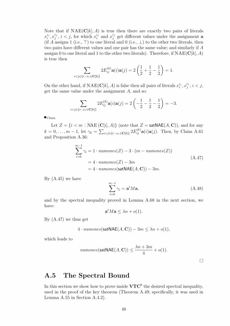
Note that if NAE(C[k], A) is true then there are exactly two pairs of literalsxεi

i , xεj

j , i < j, for which xεi

i and xεj

j get different values under the assignment a(if A assigns 1 (i.e., ⊤) to one literal and 0 (i.e., ⊥) to the other two literals, thentwo pairs have different values and one pair has the same value; and similarly if Aassigns 0 to one literal and 1 to the other two literals). Therefore, if NAE(C[k], A)is true then

∑

i<j∈r : xr∈C[k]

2E(k)ij a(i)a(j) = 2

(1

2+

1

2− 1

2

)= 1.

On the other hand, if NAE(C[k], A) is false then all pairs of literals xεi

i , xεj

j , i < j,get the same value under the assignment A, and so:

∑

i<j∈r : xr∈C[k]

2E(k)ij a(i)a(j) = 2

(−1

2− 1

2− 1

2

)= −3.

Claim

Let Z = i < m : NAE (C[i], A) (note that Z = satNAE(A,C)), and for any

k = 0, . . . ,m − 1, let γk =∑

i<j∈r : xr∈C[k] 2E(k)ij a(i)a(j). Then, by Claim A.61

and Proposition A.36:

m−1∑

i=0

γi = 1 · numones(Z)− 3 · (m− numones(Z))

= 4 · numones(Z)− 3m

= 4 · numones(satNAE(A,C))− 3m.

(A.47)

By (A.45) we havem−1∑

i=0

γi = atMa, (A.48)

and by the spectral inequality proved in Lemma A.68 in the next section, wehave:

atMa ≤ λn+ o(1).

By (A.47) we thus get

4 · numones(satNAE(A,C))− 3m ≤ λn+ o(1),

which leads to

numones(satNAE(A,C)) ≤ λn+ 3m

4+ o(1).

A.5 The Spectral Bound

In this section we show how to prove inside VTC0 the desired spectral inequality,used in the proof of the key theorem (Theorem A.49; specifically, it was used inLemma A.55 in Section A.4.2).

48

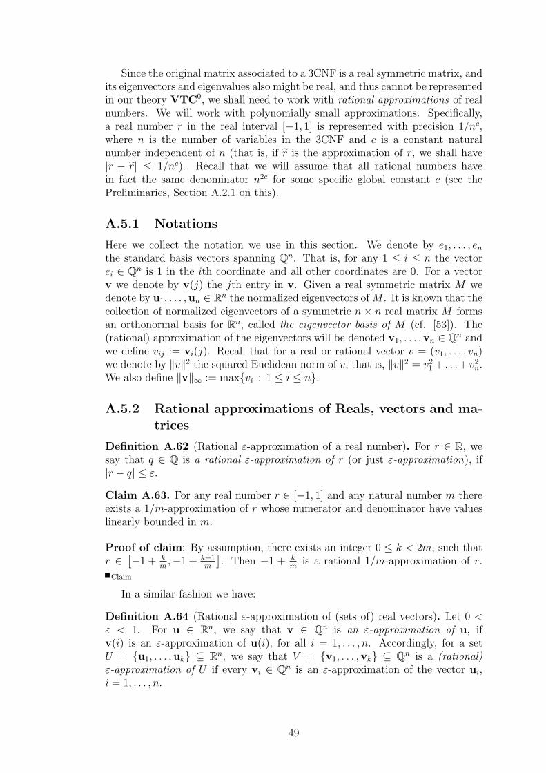
Since the original matrix associated to a 3CNF is a real symmetric matrix, andits eigenvectors and eigenvalues also might be real, and thus cannot be representedin our theory VTC0, we shall need to work with rational approximations of realnumbers. We will work with polynomially small approximations. Specifically,a real number r in the real interval [−1, 1] is represented with precision 1/nc,where n is the number of variables in the 3CNF and c is a constant naturalnumber independent of n (that is, if r is the approximation of r, we shall have|r − r| ≤ 1/nc). Recall that we will assume that all rational numbers havein fact the same denominator n2c for some specific global constant c (see thePreliminaries, Section A.2.1 on this).

A.5.1 Notations

Here we collect the notation we use in this section. We denote by e1, . . . , en

the standard basis vectors spanning Qn. That is, for any 1 ≤ i ≤ n the vectorei ∈ Qn is 1 in the ith coordinate and all other coordinates are 0. For a vectorv we denote by v(j) the jth entry in v. Given a real symmetric matrix M wedenote by u1, . . . ,un ∈ Rn the normalized eigenvectors of M . It is known that thecollection of normalized eigenvectors of a symmetric n× n real matrix M formsan orthonormal basis for Rn, called the eigenvector basis of M (cf. [53]). The(rational) approximation of the eigenvectors will be denoted v1, . . . ,vn ∈ Qn andwe define vij := vi(j). Recall that for a real or rational vector v = (v1, . . . , vn)we denote by ‖v‖2 the squared Euclidean norm of v, that is, ‖v‖2 = v2

1 + . . .+ v2n.

We also define ‖v‖∞ := maxvi : 1 ≤ i ≤ n.

A.5.2 Rational approximations of Reals, vectors and ma-trices

Definition A.62 (Rational ε-approximation of a real number). For r ∈ R, wesay that q ∈ Q is a rational ε-approximation of r (or just ε-approximation), if|r − q| ≤ ε.

Claim A.63. For any real number r ∈ [−1, 1] and any natural number m thereexists a 1/m-approximation of r whose numerator and denominator have valueslinearly bounded in m.

Proof of claim: By assumption, there exists an integer 0 ≤ k < 2m, such thatr ∈

[−1 + k

m,−1 + k+1

m

]. Then −1 + k

mis a rational 1/m-approximation of r.

Claim

In a similar fashion we have:

Definition A.64 (Rational ε-approximation of (sets of) real vectors). Let 0 <ε < 1. For u ∈ Rn, we say that v ∈ Qn is an ε-approximation of u, ifv(i) is an ε-approximation of u(i), for all i = 1, . . . , n. Accordingly, for a setU = u1, . . . ,uk ⊆ Rn, we say that V = v1, . . . ,vk ⊆ Qn is a (rational)ε-approximation of U if every vi ∈ Qn is an ε-approximation of the vector ui,i = 1, . . . , n.

49

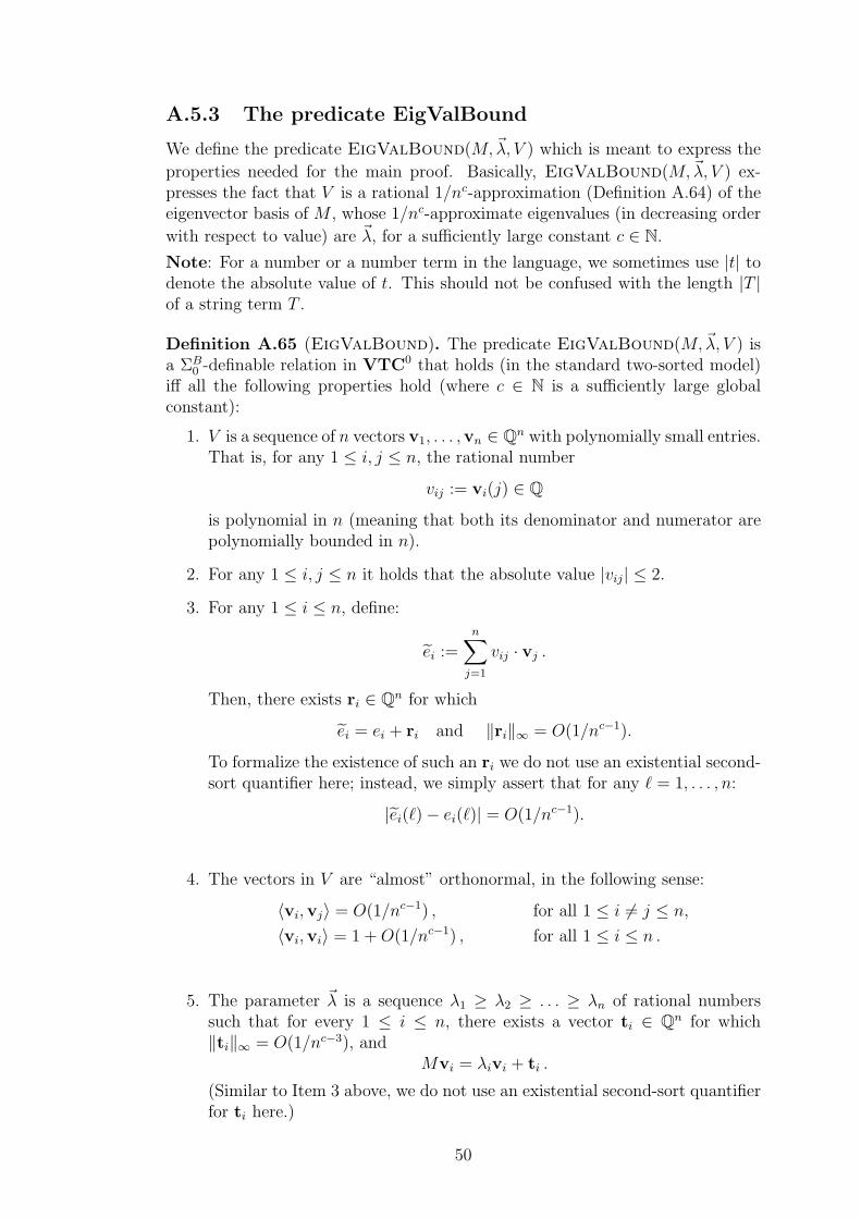
A.5.3 The predicate EigValBound

We define the predicate EigValBound(M,~λ, V ) which is meant to express the

properties needed for the main proof. Basically, EigValBound(M,~λ, V ) ex-presses the fact that V is a rational 1/nc-approximation (Definition A.64) of theeigenvector basis of M , whose 1/nc-approximate eigenvalues (in decreasing order

with respect to value) are ~λ, for a sufficiently large constant c ∈ N.

Note: For a number or a number term in the language, we sometimes use |t| todenote the absolute value of t. This should not be confused with the length |T |of a string term T .

Definition A.65 (EigValBound). The predicate EigValBound(M,~λ, V ) isa ΣB

0 -definable relation in VTC0 that holds (in the standard two-sorted model)iff all the following properties hold (where c ∈ N is a sufficiently large globalconstant):

1. V is a sequence of n vectors v1, . . . ,vn ∈ Qn with polynomially small entries.That is, for any 1 ≤ i, j ≤ n, the rational number

vij := vi(j) ∈ Q

is polynomial in n (meaning that both its denominator and numerator arepolynomially bounded in n).

2. For any 1 ≤ i, j ≤ n it holds that the absolute value |vij| ≤ 2.

3. For any 1 ≤ i ≤ n, define:

ei :=n∑

j=1

vij · vj .

Then, there exists ri ∈ Qn for which

ei = ei + ri and ‖ri‖∞ = O(1/nc−1).

To formalize the existence of such an ri we do not use an existential second-sort quantifier here; instead, we simply assert that for any ℓ = 1, . . . , n:

|ei(ℓ)− ei(ℓ)| = O(1/nc−1).

4. The vectors in V are “almost” orthonormal, in the following sense:

〈vi,vj〉 = O(1/nc−1) , for all 1 ≤ i 6= j ≤ n,

〈vi,vi〉 = 1 +O(1/nc−1) , for all 1 ≤ i ≤ n .

5. The parameter ~λ is a sequence λ1 ≥ λ2 ≥ . . . ≥ λn of rational numberssuch that for every 1 ≤ i ≤ n, there exists a vector ti ∈ Qn for which‖ti‖∞ = O(1/nc−3), and

Mvi = λivi + ti .

(Similar to Item 3 above, we do not use an existential second-sort quantifierfor ti here.)

50

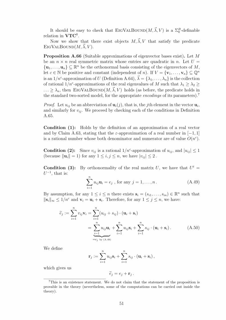
It should be easy to check that EigValBound(M,~λ, V ) is a ΣB0 -definable

relation in VTC0.Now we show that there exist objects M,~λ, V that satisfy the predicate

EigValBound(M,~λ, V ).

Proposition A.66 (Suitable approximations of eigenvector bases exist). Let Mbe an n × n real symmetric matrix whose entries are quadratic in n. Let U =u1, . . . ,un ⊆ Rn be the orthonormal basis consisting of the eigenvectors of M ,let c ∈ N be positive and constant (independent of n). If V = v1, . . . ,vn ⊆ Qn

is an 1/nc-approximation of U (Definition A.64), ~λ = λ1, . . . , λn is the collectionof rational 1/nc-approximations of the real eigenvalues of M such that λ1 ≥ λ2 ≥. . . ≥ λn, then EigValBound(M,~λ, V ) holds (as before, the predicate holds inthe standard two-sorted model, for the appropriate encodings of its parameters).7

Proof. Let uij be an abbreviation of ui(j), that is, the jth element in the vector ui,and similarly for vij. We proceed by checking each of the conditions in DefinitionA.65.

Condition (1): Holds by the definition of an approximation of a real vectorand by Claim A.63, stating that the ε-approximation of a real number in [−1, 1]is a rational number whose both denominator and numerator are of value O(nc).

Condition (2): Since vij is a rational 1/nc-approximation of uij, and |uij| ≤ 1(because ‖ui‖ = 1) for any 1 ≤ i, j ≤ n, we have |vij| ≤ 2 .

Condition (3): By orthonormality of the real matrix U , we have that U t =U−1, that is:

n∑

i=1

uijui = ej , for any j = 1, . . . , n . (A.49)

By assumption, for any 1 ≤ i ≤ n there exists si = (si1, . . . , sin) ∈ Rn such that‖si‖∞ ≤ 1/nc and vi = ui + si. Therefore, for any 1 ≤ j ≤ n, we have:

ej :=n∑

i=1

vijvi =n∑

i=1

(uij + sij) · (ui + si)

=n∑

i=1

uijui

︸ ︷︷ ︸=ej by (A.49)

+n∑

i=1

uijsi +n∑

i=1

sij · (ui + si) . (A.50)

We define

rj :=n∑

i=1

uijsi +n∑

i=1

sij · (ui + si) ,

which gives usej = ej + rj .

7This is an existence statement. We do not claim that the statement of the proposition isprovable in the theory (nevertheless, some of the computations can be carried out inside thetheory).

51

Note that since∑n

i=1 vijvi = ej is a rational vector then rj is also a rationalvector.

It remains to show that ‖rj‖∞ = O(1/nc−1). Since 1 = ‖ui‖2 =∑n

j=1 u2ij, we

have |uij| ≤ 1. By this, and by the fact that ‖si‖∞ ≤ 1/nc, we get ‖∑ni=1uijsi‖∞ =

O(1/nc−1) , and ‖∑ni=1 sij · (ui + si)‖∞ = O(1/nc−1). This means that ‖rj‖∞ =

O(1/nc−1).

Condition (4): This is similar to the proof of Condition (3). By assumption,for any 1 ≤ i ≤ n there exists si = (si1, . . . , sin) ∈ Rn such that ‖si‖∞ ≤ 1/nc,and vi = ui + si. Thus, we have

〈vi,vj〉 = 〈ui + si,uj + sj〉= 〈ui,uj〉+ 〈si,uj + sj〉+ 〈ui, sj〉 . (A.51)

The first term in (A.51) is 0 since U is an orthonormal basis, and the second andthird terms in (A.51) are both O(1/nc−1) (by calculations similar to that in theproof of Condition (3)).

The proof of 〈vi,vi〉 = 1 +O(1/nc−1) , for all 1 ≤ i ≤ n , is similar.

Condition (5): Similar to the proof of previous conditions, we define si =(si1, . . . , sin) ∈ Rn such that ‖si‖∞ ≤ 1/nc, and vi = ui + si, for any 1 ≤ i ≤ n.We have

Mvi = M(ui + si)

= Mui +Msi. (A.52)

Since ui ∈ Rn is the eigenvector of M and λi is a 1/nc-approximation of theeigenvalue of ui, we have that (A.52) equals

(λi + ǫ)ui +Msi (A.53)

for some |ǫ| ≤ 1/nc,

= λiui + ǫui +Msi

= λi(vi − si) + ǫui +Msi

= λivi − λisi + ǫui +Msi .

We putti := −λisi + ǫui +Msi.

It remains to show that ‖ti‖∞ = O(1/nc−3).

Claim A.67. For every 1 ≤ i ≤ n, λi = O(n3).

Proof of claim: Since ‖ui‖∞ = 1 and, by assumption, every entry in M isO(n2), we have:

‖Mui‖∞ = O(n3). (A.54)

Observe thatMui = (λi + ǫ)ui = λiui + ǫui. (A.55)

52

Because |ǫ| ≤ 1/nc and ‖ui‖∞ = 1, we have ‖ǫui‖∞ = O(1/nc). Therefore, by(A.54) and (A.55) we have λi = O(n3). Claim

We have ‖si‖∞ ≤ 1/nc, and so by Claim A.67 we get that ‖ − λisi‖∞ =O(1/nc−3). Now, ‖ǫui‖∞ = O(1/nc) and since M has entries which are O(n2) wehave ‖Msi‖∞ = O(1/nc−3). We conclude that

‖ti‖∞ = ‖ − λisi + ǫui +Msi‖∞≤ ‖−λisi‖∞ + ‖ǫui‖∞ + ‖Msi‖∞= O(1/nc−3).

A.5.4 Certifying the spectral inequality

In this section we show that the theory VTC0 can prove that,if EigValBound(M,~λ, V ) holds, then the desired spectral inequality also holds.

Note on coding and formalizing the proof in VTC0: In what follows wewill write freely terms such as matrices, vectors, inner products, products of amatrix by a vector (of the appropriate dimensions), addition of vectors, and bigsums. We also use freely basic properties of these objects; like transitivity ofinequalities, distributivity of a product over big sums, associativity of additionand product, etc. We showed how to formalize these objects, and how to provetheir basic properties within VTC0 in Sections A.2.2 and A.2.2 (see PropositionA.39).

For an assignment A ∈ 0, 1n we define its associated vector a ∈ −1, 1nsuch that a(i) = 1 if A(i) = 1 and a(i) = −1 if A(i) = 0. In other words wedefine a(i) = 2A(i)− 1. Note that

a =n∑

i=1

a(i) · ei .

We define

a :=n∑

i=1

a(i) · ei , (A.56)

and recall that ei :=∑n

j=1 vij · vj is a rational approximation of ei (Definition

A.65). We let atMa abbreviate 〈a,Ma〉 (which is ΣB1 -definable in VTC0, by

Section A.2.2).

Lemma A.68 (Main spectral bound). The theory VTC0 proves that if A is anassignment to n variables (that is, A is a string variable of length n + 1) and

EigValBound(M,~λ, V ) holds, then

atMa ≤ λn+ o(1) . (A.57)

This is a corollary of Lemma A.69 and Lemma A.72 that follow.

53

Lemma A.69. The theory VTC0 proves that for any assignment A to n vari-ables, EigValBound(M,~λ, V ) implies:

atMa ≤ atM a +O(1/nc−5),

where c is the constant from the EigValBound(MK , ~λ, V ) predicate.

Proof. First note that A is a string variable of length n. By Definition A.65 forany 1 ≤ j ≤ n there exists a vector rj ∈ Qn such that ej = ej + rj, and where‖rj‖∞ = O(1/nc−1). Therefore, by (A.56):

a =n∑

i=1

a(i)ei =n∑

i=1

a(i)(ei + ri) =n∑

i=1

a(i)ei +n∑

i=1

a(i)ri .

Note that∑n

i=1 a(i)ei = a, and let

r :=n∑

i=1

a(i)ri .

Then,a = a + r ,

and since a(i) ∈ −1, 1, we have ‖r‖∞ = O(1/nc−2). Now, proceed as follows:

atMa = (a− r)tM(a− r)

= atM a− atMr− rtM a + rtMr . (A.58)

We now claim that (provably in VTC0) the three right terms in (A.58) are o(1):

Claim A.70. The theory VTC0 proves that for any assignment A to n variables,EigValBound(M,~λ, V ) implies:

−atMr− rtM a + rtMr = O(1/nc−5

).

Proof of claim: Consider −atMr. Since ‖a‖∞ ≤ 2 and since (by construc-tion) each entry in M is at most O(n2), we have ‖atM‖∞ = O(n3) . There-fore, since ‖r‖∞ ≤ 1/nc−2, we get −atMr = O

(1

nc−5

). Similarly, we have

−rtM a = O(

1nc−5

).

Considering rtMr, we have ‖rtM‖∞ = O(1/nc−4) and so rtMr = O(1/nc−5 ·1/nc−2 · n) = O(1/n2c−8) = O(1/nc−5). Claim

Claim A.70 concludes the proof of Lemma A.69.

Claim A.71. There is a constant c′ such that the theory VTC0 proves thatEigValBound(M,~λ, V ) implies that:

〈ei, ei〉 = 1 +O(1/nc′), for any 1 ≤ i ≤ n, and

〈ei, ej〉 = O(1/nc′), for any 1 ≤ i 6= j ≤ n.

54

Proof of claim: By assumption for any 1 ≤ i ≤ n, ei = ei + ri for some‖ri‖∞ = O(1/nc−1). Thus

〈ei, ei〉 = 〈ei + ri, ei + ri〉= ‖ei‖2 + 2〈ei, ri〉+ ‖ri‖2 (A.59)

= 1 + o(1), (A.60)

where the last equation holds since 2〈ei, ri〉 and ‖ri‖2 can be easily proved to beo(1) in VTC0.

Proving 〈ei, ej〉 = O(1/c′) for any 1 ≤ i 6= j ≤ n, is similar. Claim

Lemma A.72. The theory VTC0 proves that for any assignment A to n vari-ables, EigValBound(M,~λ, V ) implies:

atM a ≤ λn+ o(1) . (A.61)

Proof. We have:

atM a = atM

(n∑

i=1

a(i)ei

)(by definition of a)

= atM

(n∑

i=1

(a(i) ·

n∑

j=1

vjivj

))(by definition of ei)

= at

n∑

i=1

(a(i) ·

n∑

j=1

vjiMvj

)(rearranging)

= at

n∑

i=1

(a(i) ·

n∑

j=1

vji(λjvj + rj)

)(by Definition A.65)

= at

n∑

i=1

(a(i) ·

n∑

j=1

λjvjivj

)+ at

n∑

i=1

(a(i) ·

n∑

j=1

vjirj

)

︸ ︷︷ ︸Term 1

(rearranging)

(A.62)

We claim (inside VTC0) that the Term 1 above is of size o(1):

Claim A.73. The theory VTC0 proves that for any assignment A to n variables,EigValBound(M,~λ, V ) implies

at

n∑

i=1

(a(i) ·

n∑

j=1

vjirj

)= O(1/nc−6) .

Proof of claim: The proof is similar to the proof of Claim A.70. Specifically,by Definition A.65, for any 1 ≤ j ≤ n, we have ‖rj‖∞ ≤ 1/nc−1, and for any1 ≤ i, j ≤ n, we have |vji| ≤ 2. Thus, VTC0 proves that ‖∑n

j=1 vjirj‖∞ =

O(1/nc−2) , for any 1 ≤ i ≤ n. Since a(i) ∈ −1, 1, for any 1 ≤ i ≤ n, the

55

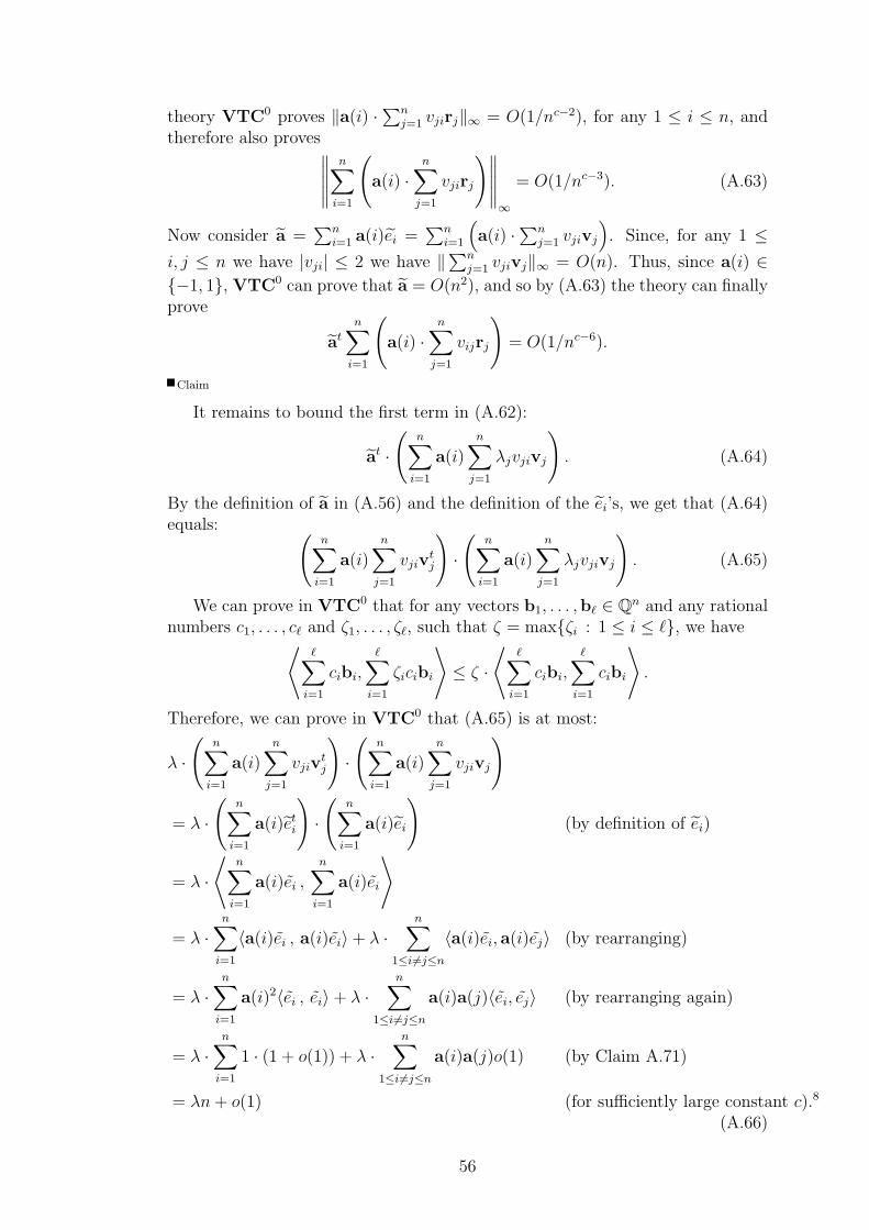
theory VTC0 proves ‖a(i) ·∑nj=1 vjirj‖∞ = O(1/nc−2), for any 1 ≤ i ≤ n, and

therefore also proves∥∥∥∥∥

n∑

i=1

(a(i) ·

n∑

j=1

vjirj

)∥∥∥∥∥∞

= O(1/nc−3). (A.63)

Now consider a =∑n

i=1 a(i)ei =∑n

i=1

(a(i) ·∑n

j=1 vjivj

). Since, for any 1 ≤

i, j ≤ n we have |vji| ≤ 2 we have ‖∑nj=1 vjivj‖∞ = O(n). Thus, since a(i) ∈

−1, 1, VTC0 can prove that a = O(n2), and so by (A.63) the theory can finallyprove

at

n∑

i=1

(a(i) ·

n∑

j=1

vijrj

)= O(1/nc−6).

Claim

It remains to bound the first term in (A.62):

at ·(

n∑

i=1

a(i)n∑

j=1

λjvjivj

). (A.64)

By the definition of a in (A.56) and the definition of the ei’s, we get that (A.64)equals: (

n∑

i=1

a(i)n∑

j=1

vjivtj

)·(

n∑

i=1

a(i)n∑

j=1

λjvjivj

). (A.65)

We can prove in VTC0 that for any vectors b1, . . . ,bℓ ∈ Qn and any rationalnumbers c1, . . . , cℓ and ζ1, . . . , ζℓ, such that ζ = maxζi : 1 ≤ i ≤ ℓ, we have

⟨ℓ∑

i=1

cibi,

ℓ∑

i=1

ζicibi

⟩≤ ζ ·

⟨ℓ∑

i=1

cibi,

ℓ∑

i=1

cibi

⟩.

Therefore, we can prove in VTC0 that (A.65) is at most:

λ ·(

n∑

i=1

a(i)n∑

j=1

vjivtj

)·(

n∑

i=1

a(i)n∑

j=1

vjivj

)

= λ ·(

n∑

i=1

a(i)eti

)·(

n∑

i=1

a(i)ei

)(by definition of ei)

= λ ·⟨

n∑

i=1

a(i)ei ,

n∑

i=1

a(i)ei

⟩

= λ ·n∑

i=1

〈a(i)ei , a(i)ei〉+ λ ·n∑

1≤i6=j≤n

〈a(i)ei, a(i)ej〉 (by rearranging)

= λ ·n∑

i=1

a(i)2〈ei , ei〉+ λ ·n∑

1≤i6=j≤n

a(i)a(j)〈ei, ej〉 (by rearranging again)

= λ ·n∑

i=1

1 · (1 + o(1)) + λ ·n∑

1≤i6=j≤n

a(i)a(j)o(1) (by Claim A.71)

= λn+ o(1) (for sufficiently large constant c).8

(A.66)

56

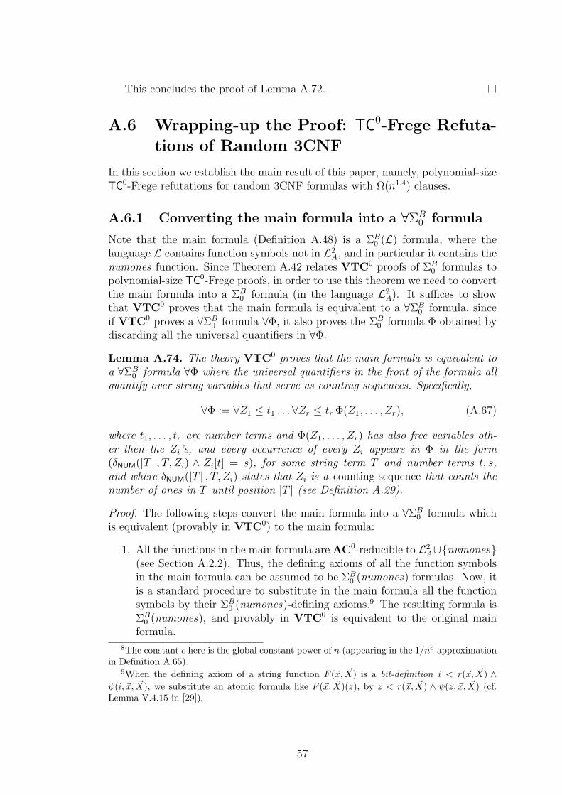
This concludes the proof of Lemma A.72.

A.6 Wrapping-up the Proof: TC0-Frege Refuta-

tions of Random 3CNF

In this section we establish the main result of this paper, namely, polynomial-sizeTC0-Frege refutations for random 3CNF formulas with Ω(n1.4) clauses.

A.6.1 Converting the main formula into a ∀ΣB0 formula

Note that the main formula (Definition A.48) is a ΣB0 (L) formula, where the

language L contains function symbols not in L2A, and in particular it contains the

numones function. Since Theorem A.42 relates VTC0 proofs of ΣB0 formulas to

polynomial-size TC0-Frege proofs, in order to use this theorem we need to convertthe main formula into a ΣB

0 formula (in the language L2A). It suffices to show

that VTC0 proves that the main formula is equivalent to a ∀ΣB0 formula, since

if VTC0 proves a ∀ΣB0 formula ∀Φ, it also proves the ΣB

0 formula Φ obtained bydiscarding all the universal quantifiers in ∀Φ.

Lemma A.74. The theory VTC0 proves that the main formula is equivalent toa ∀ΣB

0 formula ∀Φ where the universal quantifiers in the front of the formula allquantify over string variables that serve as counting sequences. Specifically,

∀Φ := ∀Z1 ≤ t1 . . . ∀Zr ≤ tr Φ(Z1, . . . , Zr), (A.67)

where t1, . . . , tr are number terms and Φ(Z1, . . . , Zr) has also free variables oth-er then the Zi’s, and every occurrence of every Zi appears in Φ in the form(δNUM(|T | , T, Zi) ∧ Zi[t] = s), for some string term T and number terms t, s,and where δNUM(|T | , T, Zi) states that Zi is a counting sequence that counts thenumber of ones in T until position |T | (see Definition A.29).

Proof. The following steps convert the main formula into a ∀ΣB0 formula which

is equivalent (provably in VTC0) to the main formula:

1. All the functions in the main formula are AC0-reducible to L2A∪numones

(see Section A.2.2). Thus, the defining axioms of all the function symbolsin the main formula can be assumed to be ΣB

0 (numones) formulas. Now, itis a standard procedure to substitute in the main formula all the functionsymbols by their ΣB

0 (numones)-defining axioms.9 The resulting formula isΣB

0 (numones), and provably in VTC0 is equivalent to the original mainformula.

8The constant c here is the global constant power of n (appearing in the 1/nc-approximationin Definition A.65).

9When the defining axiom of a string function F (~x, ~X) is a bit-definition i < r(~x, ~X) ∧ψ(i, ~x, ~X), we substitute an atomic formula like F (~x, ~X)(z), by z < r(~x, ~X) ∧ ψ(z, ~x, ~X) (cf.Lemma V.4.15 in [29]).

57

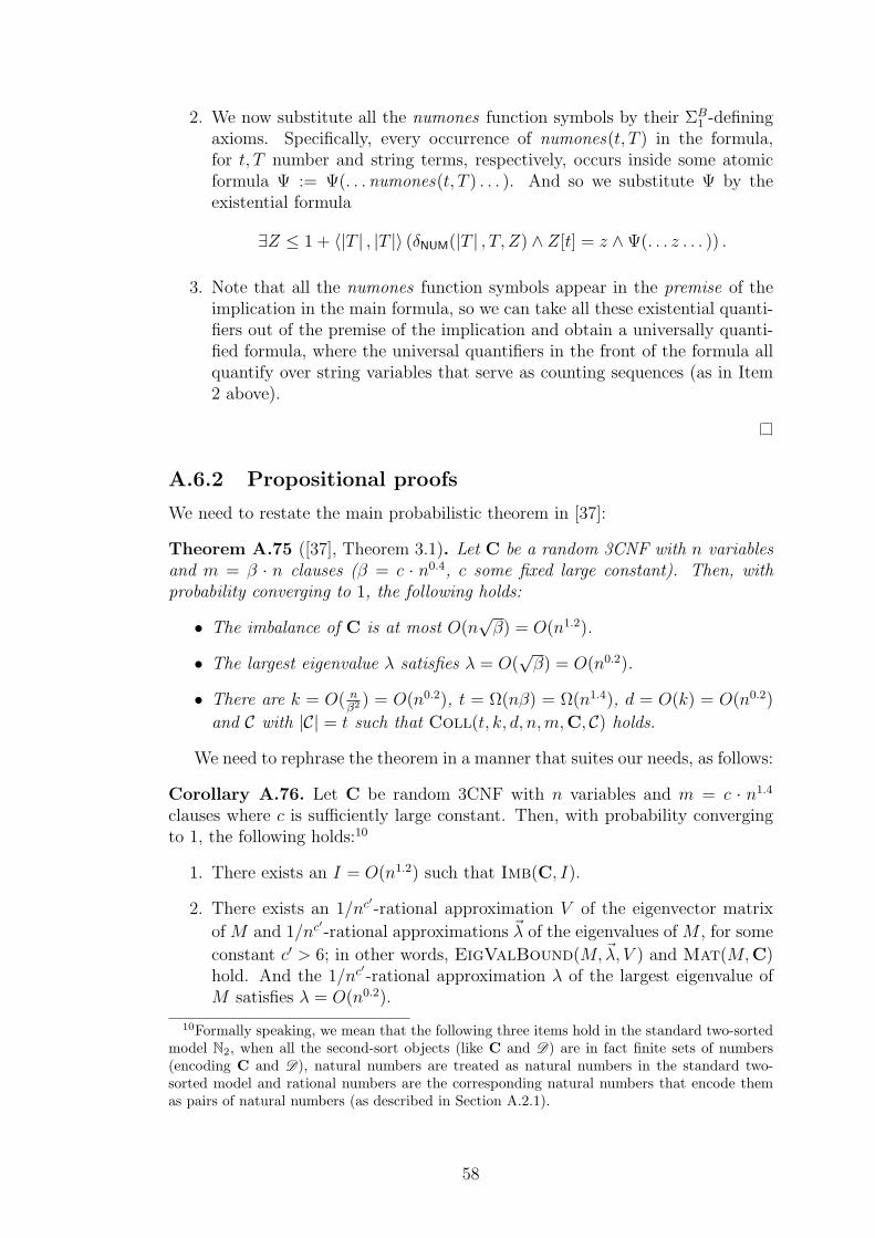
2. We now substitute all the numones function symbols by their ΣB1 -defining

axioms. Specifically, every occurrence of numones(t, T ) in the formula,for t, T number and string terms, respectively, occurs inside some atomicformula Ψ := Ψ(. . . numones(t, T ) . . . ). And so we substitute Ψ by theexistential formula

∃Z ≤ 1 + 〈|T | , |T |〉 (δNUM(|T | , T, Z) ∧ Z[t] = z ∧Ψ(. . . z . . . )) .

3. Note that all the numones function symbols appear in the premise of theimplication in the main formula, so we can take all these existential quanti-fiers out of the premise of the implication and obtain a universally quanti-fied formula, where the universal quantifiers in the front of the formula allquantify over string variables that serve as counting sequences (as in Item2 above).

A.6.2 Propositional proofs

We need to restate the main probabilistic theorem in [37]:

Theorem A.75 ([37], Theorem 3.1). Let C be a random 3CNF with n variablesand m = β · n clauses (β = c · n0.4, c some fixed large constant). Then, withprobability converging to 1, the following holds:

• The imbalance of C is at most O(n√β) = O(n1.2).

• The largest eigenvalue λ satisfies λ = O(√β) = O(n0.2).

• There are k = O( nβ2 ) = O(n0.2), t = Ω(nβ) = Ω(n1.4), d = O(k) = O(n0.2)

and C with |C| = t such that Coll(t, k, d, n,m,C, C) holds.

We need to rephrase the theorem in a manner that suites our needs, as follows:

Corollary A.76. Let C be random 3CNF with n variables and m = c · n1.4

clauses where c is sufficiently large constant. Then, with probability convergingto 1, the following holds:10

1. There exists an I = O(n1.2) such that Imb(C, I).

2. There exists an 1/nc′-rational approximation V of the eigenvector matrix

of M and 1/nc′-rational approximations ~λ of the eigenvalues of M , for some

constant c′ > 6; in other words, EigValBound(M,~λ, V ) and Mat(M,C)hold. And the 1/nc′-rational approximation λ of the largest eigenvalue ofM satisfies λ = O(n0.2).

10Formally speaking, we mean that the following three items hold in the standard two-sortedmodel N2, when all the second-sort objects (like C and D) are in fact finite sets of numbers(encoding C and D), natural numbers are treated as natural numbers in the standard two-sorted model and rational numbers are the corresponding natural numbers that encode themas pairs of natural numbers (as described in Section A.2.1).

58

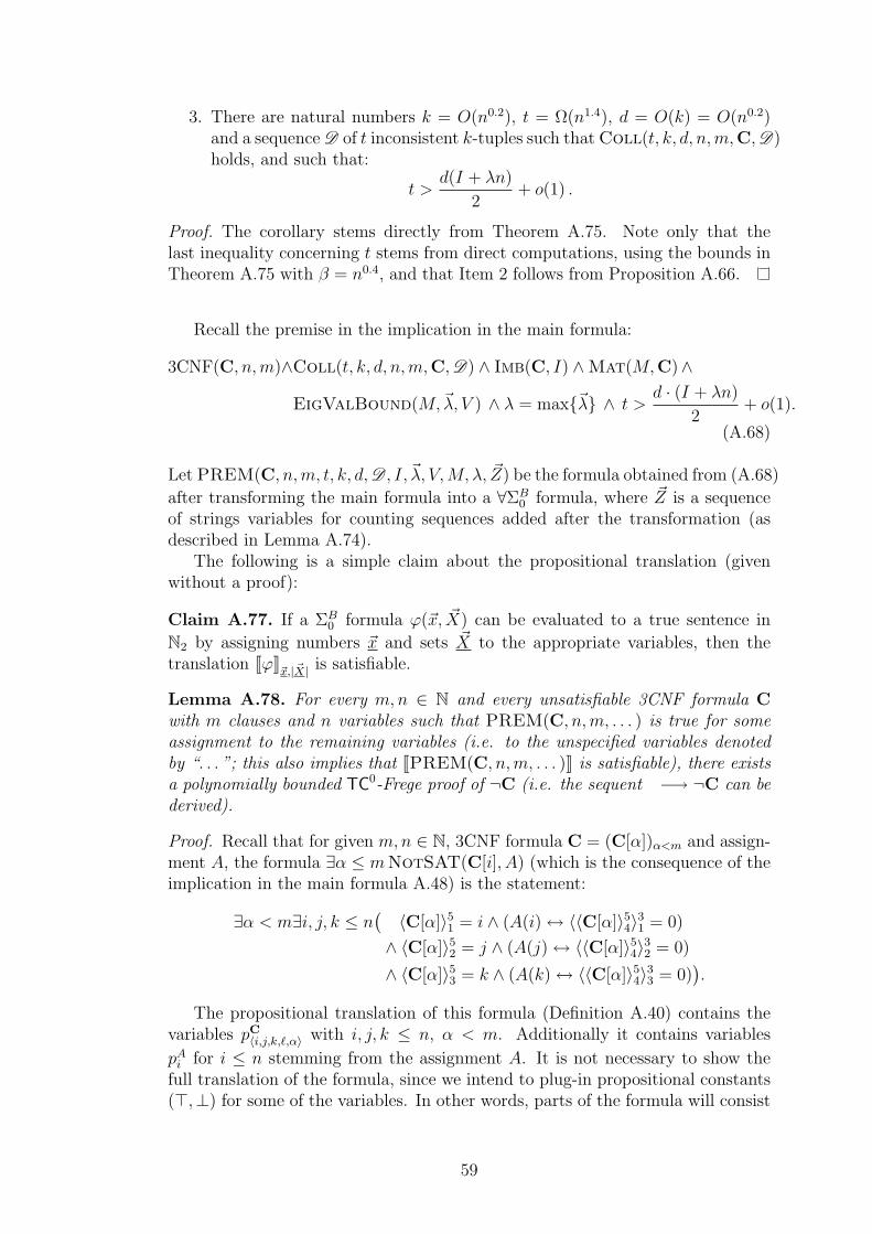
3. There are natural numbers k = O(n0.2), t = Ω(n1.4), d = O(k) = O(n0.2)and a sequence D of t inconsistent k-tuples such that Coll(t, k, d, n,m,C,D)holds, and such that:

t >d(I + λn)

2+ o(1) .

Proof. The corollary stems directly from Theorem A.75. Note only that thelast inequality concerning t stems from direct computations, using the bounds inTheorem A.75 with β = n0.4, and that Item 2 follows from Proposition A.66.

Recall the premise in the implication in the main formula:

3CNF(C, n,m)∧Coll(t, k, d, n,m,C,D) ∧ Imb(C, I) ∧Mat(M,C)∧

EigValBound(M,~λ, V ) ∧ λ = max~λ ∧ t >d · (I + λn)

2+ o(1).

(A.68)

Let PREM(C, n,m, t, k, d,D , I, ~λ, V,M, λ, ~Z) be the formula obtained from (A.68)

after transforming the main formula into a ∀ΣB0 formula, where ~Z is a sequence

of strings variables for counting sequences added after the transformation (asdescribed in Lemma A.74).

The following is a simple claim about the propositional translation (givenwithout a proof):

Claim A.77. If a ΣB0 formula ϕ(~x, ~X) can be evaluated to a true sentence in

N2 by assigning numbers ~x and sets ~X to the appropriate variables, then thetranslation JϕK

~x, ~|X|is satisfiable.

Lemma A.78. For every m,n ∈ N and every unsatisfiable 3CNF formula Cwith m clauses and n variables such that PREM(C, n,m, . . . ) is true for someassignment to the remaining variables (i.e. to the unspecified variables denotedby “. . . ”; this also implies that JPREM(C, n,m, . . . )K is satisfiable), there existsa polynomially bounded TC0-Frege proof of ¬C (i.e. the sequent −→ ¬C can bederived).

Proof. Recall that for given m,n ∈ N, 3CNF formula C = (C[α])α<m and assign-ment A, the formula ∃α ≤ mNotSAT(C[i], A) (which is the consequence of theimplication in the main formula A.48) is the statement:

∃α < m∃i, j, k ≤ n(〈C[α]〉51 = i ∧ (A(i)↔ 〈〈C[α]〉54〉31 = 0)

∧ 〈C[α]〉52 = j ∧ (A(j)↔ 〈〈C[α]〉54〉32 = 0)

∧ 〈C[α]〉53 = k ∧ (A(k)↔ 〈〈C[α]〉54〉33 = 0)).

The propositional translation of this formula (Definition A.40) contains thevariables pC〈i,j,k,ℓ,α〉 with i, j, k ≤ n, α < m. Additionally it contains variables

pAi for i ≤ n stemming from the assignment A. It is not necessary to show the

full translation of the formula, since we intend to plug-in propositional constants(⊤,⊥) for some of the variables. In other words, parts of the formula will consist

59

of only constants and so it is unnecessary to give these parts in full detail. Havingthis in mind, the translation J∃α < mNotSAT(C[α], A)Km,n is

m−1∨

α=0

n∨

i,j,k=1

( (J〈C[α]〉51 = iKm,n ∧ (pAi ↔ J〈〈C[α]〉54〉31 = 0Km,n))

∧ (〈J〈C[α]〉52 = jKm,n ∧ (pAj ↔ J〈〈C[α]〉54〉32 = 0Km,n))

∧ (〈J〈C[α]〉53 = kKm,n ∧ (pAk ↔ J〈〈C[α]〉54〉33 = 0Km,n))).

(A.69)

Here, the variables pC〈i,j,k,ℓ,α〉 all implicitly appear in the parts inside J·K.Now assume we have a fixed 3CNF C with n variables andm clauses. Then for

every α < m there exists 1 ≤ i, j, k ≤ n such that the formulas J〈C[α]〉51 = iKm,n

and J〈C[α]〉52 = jKm,n and J〈C[α]〉53 = kKm,n are all satisfied (in fact they arepolynomial-size in n propositional tautologies consisting of only constants ⊤,⊥).From now on we will only concentrate on the disjuncts where this is the case(as the other disjuncts are falsified, or in other words they are propositionalcontradictions consisting of only constants).

By plugging C into J〈〈C[α]〉54〉31 = 0Km,n and J〈〈C[α]〉54〉32 = 0Km,n and J〈〈C[α]〉54〉33 =0Km,n we get that J∃α < mNotSAT(C[α], A)Km,n is evaluated to

∨

α<m

((pA

i )ℓα1 ∧ (pA

j )ℓα2 ∧ (pA

k )ℓα3), (A.70)

where ℓαr is an abbreviation of J〈〈C[α]〉54〉3r = 0Km,n, and thus we can observe that

(A.70) gets evaluated to ¬C(pA1 /x1, . . . , p

An/xn), where pA

i /xi means substitutionof xi by pA

i .

By Theorem A.49 the theory VTC0 proves the main formula and so by Lem-ma A.74 there is a VTC0 proof of

PREM(C, n,m, t, k, d,D , I, ~λ, V,M, λ, ~Z)→ ∃i < mNotSAT(C[i], A).

Thus, by Theorem A.42 we can derive a polynomially bounded TC0-proof of theformula

JPREM(C, . . . )Km,n → J∃α < mNotSAT(C[α], A)Km,n

and thus also of the sequent

JPREM(C, . . . )Km,n −→ J∃α < mNotSAT(C[α], A)Km,n.

By Claim A.77 and the assumption that PREM(C, n,m, . . . ) is true in N2 foran assignment to the remaining variables we know that JPREM(C, . . . )Km,n issatisfiable. Plugging-in such a satisfying assignment ~a into JPREM(C, . . . )Km,n,Lemma A.17 yields a polynomially bounded TC0-Frege proof of

JPREM(C,~a)Km,n

and of the sequent

JPREM(C,~a)Km,n −→ J∃α < mNotSAT(C[α], A)Km,n.

60

Using the Cut rule (Definition A.14) we get a polynomially bounded TC0-Fregeproof of the formula

J∃α < mNotSAT(C[α], A)Km,n.

As we showed before, this gets evaluated to

¬C(pA1 /x1, . . . , p

An/xn)

as desired. Because of Claim A.17, this proof is only polynomially longer thanthe one of the translation of the main formula. Since that proof was polynomiallybounded, the above proof of ¬C(pA

i /xi) also is.

We can now conclude:

Corollary A.79. With probability converging to 1, a random 3CNF C withn variables and m ≥ c · n1.4 clauses, c a sufficiently large constant, ¬C haspolynomially bounded TC0-Frege proofs, while C has no sub-exponential sizeresolution refutations (as long as m = O(n1.5−ǫ), for 0 < ǫ < 1/2).

Proof. By Corollary A.76, with probability converging to 1 there exists an as-signment of numbers and strings ~α (including also the appropriate counting se-quences assigned to the Zi string variables introduced in Lemma A.74) such thatPREM(C, ~α) holds (in the standard two-sorted model). Therefore, with prob-ability converging to 1 we can apply Lemma A.78 to establish that ¬C has ashort TC0-Frege proof. That with probability converging to 1 there are no sub-exponential size resolution refutations of C follows from [25, 10, 15].

A.7 Acknowledgments

We wish to thank Jan Krajıcek for very helpful discussions concerning the topicof this paper and for commenting on an earlier manuscript and Emil Jerabekand Neil Thapen for answering many of our questions about theories of weakarithmetic and for many other insightful comments.

61

B. Polylogarithmic Cuts ofModels of V0

B.1 Introduction

This article is on the one hand on models of weak arithmetics and on the otheron proof complexity, i.e. the question of how long formal proofs of tautologieshave to be in given proof systems. Therefore the introduction will consist of twoparts, one for each subject.

Models of weak arithmetics, like I∆0, have been extensively studied for severalreasons, possibly being the simplest objects whose theories bear enough strengthto do a good part of mathematics in and still are weak enough to allow for a certainkind of constructiveness. The latter has been demonstrated over and over againby various results connecting weak arithmetic theories with complexity classesand computability. We are interested in the strength of the theory obtained byrestricting our objects of reasoning to a small initial part of a given model. Sincea two-sorted theory, such as V0, is much stronger on its number part than onits set part, it is likely that such a cut is a model of a supposedly much strongertheory. Indeed we will see in Section B.3 that certain cuts of models of V0 aremodels of the provably stronger theory VNC1. This strengthens a result by Parisand Wilkie [75][74], who show that such cuts are models of VTC0. In fact theywork in a more general setting and, following our argumentation, their resultreadily implies the sub exponential simulation of TC0-Frege by AC0-Frege fromBonet, Domingo, Gavalda, Maciel, and Pitassi [17].

Proof Complexity, on the other hand, more or less began when Cook andReckhow [30] discovered the close connection between the lengths of formal proofsin propositional proof systems and standard complexity classes. This connectionyields a possibility of dealing with the coNP/NP question by asking, whetherthere exists a propositional proof system that is polynomially bounded. We willnot directly address this question here, but rather explore the relative strengths oftwo major proof systems, Frege and bounded depth Frege. These proof systemshave been extensively studied, due to their natural appearance as classical calculi,such as Gentzen’s PK, and it is well known that Frege systems are stronger thanbounded depth Frege systems, as the former system has polynomial size proofsfor the Pigeonhole Principle (see [21]), while the latter does not (see [62] and[78]). Lately, Filmus, Pitassi and Santhanam [39] have proved a sub exponentialsimulation of Frege by bounded depth Frege using a combinatoric argument. InSection B.4 we will obtain the same result by an application of our result aboutcuts to the provability of the Reflection Principle for Frege in bounded depthFrege. Currently Cook, Ghasemloo and Nguyen [28] are working on a purelysyntactical proof that gives a slightly better result with respect to the strengthof the simulated proof system.

The paper is built-up as follows. In section B.2 we briefly recapture somebasics about Complexity Theory, Bounded Arithmetic, Proof Complexity and thevarious connections between them. As this is only expository it might be helpfulto consult some of the references for a more detailed introduction (see [5], [29]

62

and [57]). After that, in Section B.3 we prove a formalization of Nepomnjascij’sTheorem in the polylogarithmic cut of a model of V0. Using a standard algorithmfor evaluating circuits and then applying the formalized version of Nepomnjascij’sTheorem we can conclude that this cut is indeed a model of VNC1. Finally, inSection B.4, we apply this result to prove that a version of the Bounded ReflectionPrinciple of Frege is provable in V0. This, together with a standard argumentlinking the provability of Reflection Principles with simulation results, yields thesub exponential simulation of Frege by bounded depth Frege.

B.2 Preliminaries

We assume familiarity with Turing machines, circuits and standard complexityclasses such as P, NP, TimeSpace(f, g), NCi, ACi and so on. See for example [5]for an introduction. We will not work a lot within these classes, but rather applyknown relations between such classes and weak arithmetic theories.

We will work in a two-sorted arithmetic setting, having one sort of variablesrepresenting numbers and the second sort representing bounded sets of numbers.We identify such bounded subsets with strings. See [29] for a thorough introduc-tion. The underlying language, denoted L2

A, consists of the following relation,function and constant symbols:

+, ·,≤, 0, 1, |·| ,=1,=2,∈ .

An L2A-structure M consists of a first-sort universe UM

1 of numbers and asecond-sort universe UM

2 of bounded subsets of numbers. If M is a model of thetwo-sorted theory V0 (see B.2.2), then the functions + and · are the additionand multiplication on the universe of numbers. 0 and 1 are interpreted as theappropriate elements zero and one with respect to addition and multiplication.The relation ≤ is an ordering relation on the first-sort universe. The function |·|maps an element of the set sort to its largest element plus one (i.e. to an elementof the number sort). The relation =1 is interpreted as equality between numbers,=2 is interpreted as equality between bounded sets of numbers. The relation ∈holds for a number n and a set of numbers N if and only if n is an element of N .The standard model of two-sorted Peano Arithmetic will be denoted as N2. Itconsists of a first-sort universe U1 = N and a second-sort universe U2 of all finitesubsets of N. The symbols are interpreted in the usual way.

We denote the first-sort (number) variables by lower-case letters x, y, z, ...,and the second-sort (set) variables by capital letters X,Y, Z, .... We can buildformulas in the usual way, using two sorts of quantifiers, number quantifiers andstring quantifiers. A number quantifier ∃x (∀x) is bounded if it is of the form∃x(x ≤ f ∧ . . . ) (∀x(x ≤ f → . . . )) for some number term f . A string quantifier∃X (∀X) is bounded if it is of the form ∃X(|X| ≤ f ∧ . . . ) (∀X(|X| ≤ f → . . . ))for some number term f . A formula is bounded iff all its quantifiers are. Allformulas in this paper will be bounded. A formula ϕ is in ΣB

0 (or ΠB0 ) if it uses

no string quantifiers and all number quantifiers are bounded. A formula ϕ isa ΣB

i+1 (or ΠBi+1) if it is of the form ∃X1 ≤ p(n) . . . ∃Xm ≤ p(n)ψ (or ∀X1 ≤

p(n) . . . ∀Xm ≤ p(n)ψ), where ψ ∈ ΠBi (or ψ ∈ ΣB

i , respectively). If a relationor predicate can be defined by both a ΣB

i and a ΠBi formula, then we call it ∆B

i

63

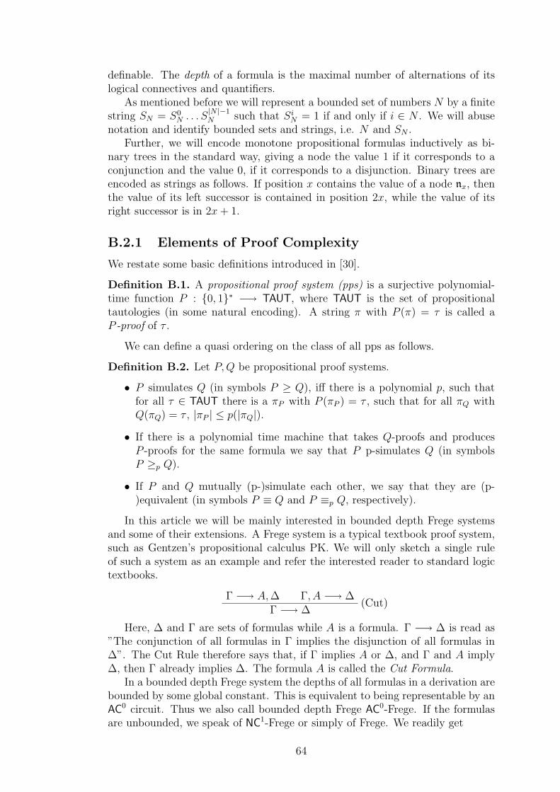
definable. The depth of a formula is the maximal number of alternations of itslogical connectives and quantifiers.

As mentioned before we will represent a bounded set of numbers N by a finitestring SN = S0

N . . . S|N |−1N such that Si

N = 1 if and only if i ∈ N . We will abusenotation and identify bounded sets and strings, i.e. N and SN .

Further, we will encode monotone propositional formulas inductively as bi-nary trees in the standard way, giving a node the value 1 if it corresponds to aconjunction and the value 0, if it corresponds to a disjunction. Binary trees areencoded as strings as follows. If position x contains the value of a node nx, thenthe value of its left successor is contained in position 2x, while the value of itsright successor is in 2x+ 1.

B.2.1 Elements of Proof Complexity

We restate some basic definitions introduced in [30].

Definition B.1. A propositional proof system (pps) is a surjective polynomial-time function P : 0, 1∗ −→ TAUT, where TAUT is the set of propositionaltautologies (in some natural encoding). A string π with P (π) = τ is called aP -proof of τ .

We can define a quasi ordering on the class of all pps as follows.

Definition B.2. Let P,Q be propositional proof systems.

• P simulates Q (in symbols P ≥ Q), iff there is a polynomial p, such thatfor all τ ∈ TAUT there is a πP with P (πP ) = τ , such that for all πQ withQ(πQ) = τ , |πP | ≤ p(|πQ|).

• If there is a polynomial time machine that takes Q-proofs and producesP -proofs for the same formula we say that P p-simulates Q (in symbolsP ≥p Q).

• If P and Q mutually (p-)simulate each other, we say that they are (p-)equivalent (in symbols P ≡ Q and P ≡p Q, respectively).

In this article we will be mainly interested in bounded depth Frege systemsand some of their extensions. A Frege system is a typical textbook proof system,such as Gentzen’s propositional calculus PK. We will only sketch a single ruleof such a system as an example and refer the interested reader to standard logictextbooks.

Γ −→ A,∆ Γ, A −→ ∆(Cut)

Γ −→ ∆

Here, ∆ and Γ are sets of formulas while A is a formula. Γ −→ ∆ is read as”The conjunction of all formulas in Γ implies the disjunction of all formulas in∆”. The Cut Rule therefore says that, if Γ implies A or ∆, and Γ and A imply∆, then Γ already implies ∆. The formula A is called the Cut Formula.

In a bounded depth Frege system the depths of all formulas in a derivation arebounded by some global constant. This is equivalent to being representable by anAC0 circuit. Thus we also call bounded depth Frege AC0-Frege. If the formulasare unbounded, we speak of NC1-Frege or simply of Frege. We readily get

64

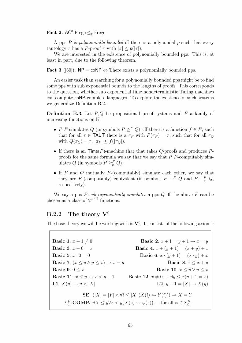
Fact 2. AC0-Frege ≤p Frege.

A pps P is polynomially bounded iff there is a polynomial p such that everytautology τ has a P -proof π with |π| ≤ p(|τ |).

We are interested in the existence of polynomially bounded pps. This is, atleast in part, due to the following theorem.

Fact 3 ([30]). NP = coNP⇔ There exists a polynomially bounded pps.

An easier task than searching for a polynomially bounded pps might be to findsome pps with sub exponential bounds to the lengths of proofs. This correspondsto the question, whether sub exponential time nondeterministic Turing machinescan compute coNP-complete languages. To explore the existence of such systemswe generalize Definition B.2.

Definition B.3. Let P,Q be propositional proof systems and F a family ofincreasing functions on N.

• P F -simulates Q (in symbols P ≥F Q), iff there is a function f ∈ F , suchthat for all τ ∈ TAUT there is a πP with P (πP ) = τ , such that for all πQ

with Q(πQ) = τ , |πP | ≤ f(|πQ|).

• If there is an Time(F )-machine that that takes Q-proofs and produces P -proofs for the same formula we say that we say that P F -computably sim-ulates Q (in symbols P ≥F

p Q).

• If P and Q mutually F -(computably) simulate each other, we say thatthey are F -(computably) equivalent (in symbols P ≡F Q and P ≡F

p Q,respectively).

We say a pps P sub exponentially simulates a pps Q iff the above F can bechosen as a class of 2no(1)

functions.

B.2.2 The theory V0

The base theory we will be working with is V0. It consists of the following axioms:

Basic 1. x+ 1 6= 0 Basic 2. x+ 1 = y + 1→ x = y

Basic 3. x+ 0 = x Basic 4. x+ (y + 1) = (x+ y) + 1

Basic 5. x · 0 = 0 Basic 6. x · (y + 1) = (x · y) + x

Basic 7. (x ≤ y ∧ y ≤ x)→ x = y Basic 8. x ≤ x+ y

Basic 9. 0 ≤ x Basic 10. x ≤ y ∨ y ≤ x

Basic 11. x ≤ y ↔ x < y + 1 Basic 12. x 6= 0→ ∃y ≤ x(y + 1 = x)

L1. X(y)→ y < |X| L2. y + 1 = |X| → X(y)

SE. (|X| = |Y | ∧ ∀i ≤ |X| (X(i)↔ Y (i)))→ X = Y

ΣB0 -COMP. ∃X ≤ y∀z < y(X(z)↔ ϕ(z)) , for all ϕ ∈ ΣB

0 .

65

Here, the Axioms Basic 1 through Basic 12 are the usual axioms used to definePeano Arithmetic without induction (PA−), which settle the basic properties ofAddition, Multiplication, Ordering, and of the constants 0 and 1. The Axiom L1says that the length of a string coding a finite set is an upper bound to the sizeof its elements. L2 says that |X| gives the largest element of X plus 1. SE is theextensionality axiom for strings which states that two strings are equal if theycode the same sets. Finally, ΣB

0 -COMP is the comprehension axiom schema forΣB

0 -formulas (it is an axiom for each such formula) and implies the existence ofall sets, which contain exactly the elements that fulfill any given ΣB

0 property.

Fact 4. The theory V0 proves the Induction Axiom schema for ΣB0 formulas Φ:

(Φ(0) ∧ ∀x(Φ(x)→ Φ(x+ 1)))→ ∀zΦ(z).

When speaking about theories we will always assume that the theories aretwo-sorted theories as in [29]).

The following is a basic notion:

Definition B.4 (Two-sorted definability). Let T be a theory over the languageL ⊇ L2

A and let Φ be a set of formulas in the language L. A number function

f is Φ-definable in a theory T iff there is a formula ϕ(~x, y, ~X) in Φ such that Tproves

∀~x∀ ~X∃!yϕ(~x, y, ~X)

and it holds thaty = f(~x, ~X)↔ ϕ(~x, y, ~X). (B.1)

A string function F is Φ-definable in a theory T iff there is a formula ϕ(~x, ~X, Y )in Φ such that T proves

∀~x∀ ~X∃!Y ϕ(~x, ~X, Y )

and it holds thatY = F (~x, ~X)↔ ϕ(~x, ~X, Y ). (B.2)

Finally, a relation R(~x, ~X) is Φ-definable iff there is a formula ϕ(~x, ~X) in Φ suchthat it holds that

R(~x, ~X)↔ ϕ(~x, ~X). (B.3)

Moreover we wish to talk about sequences coded by strings or numbers. For astring X we let X[i] be the ith bit of X. Assuming a tupling function 〈·, . . . , ·〉 wecan also talk of k-ary relations in the obvious way by referring to X[〈i0, . . . , ik〉].For the sake of simplicity we also refer to X[〈i0, . . . , ik〉] by X[i0, . . . , ik].

Using k-ary relations we can also encode sequences of bounded numbersx0, . . . , xm by xi = X[〈i, 0〉]X[〈i, 1〉] . . . X[〈i, k〉] in binary. Matrices and so oncan obviously be formalized in the same way.

Given a string X[〈x1, . . . , xk〉] representing a k-ary relation, we denote the k−ℓ-ary substring with parameters ai1 , . . . , aiℓ by X[〈·, . . . , ·, ai1 , ·, . . . , aiℓ , ·, . . . , ·〉].For example we refer to the element aij of a given matrix A[〈x1, x2, x3〉] asA[〈i, j, ·〉], a string representing aij in binary. Observe that this substring canbe ΣB

0 defined in V0.Given a number x we denote by 〈x〉j the jth number in the sequence encoded

by x. To do this we assume a fixed ΣB0 definable encoding of numbers that is 1-1.

66

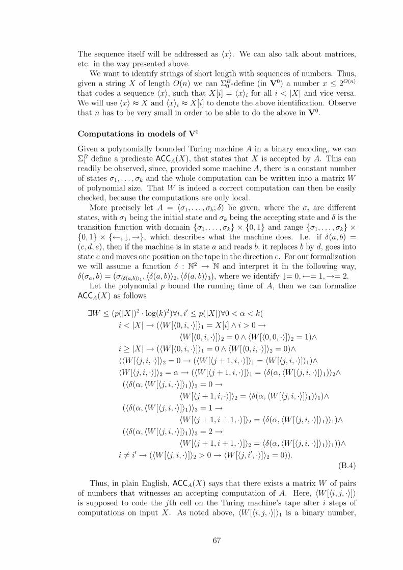
The sequence itself will be addressed as 〈x〉. We can also talk about matrices,etc. in the way presented above.

We want to identify strings of short length with sequences of numbers. Thus,given a string X of length O(n) we can ΣB

0 -define (in V0) a number x ≤ 2O(n)

that codes a sequence 〈x〉, such that X[i] = 〈x〉i for all i < |X| and vice versa.We will use 〈x〉 ≈ X and 〈x〉i ≈ X[i] to denote the above identification. Observethat n has to be very small in order to be able to do the above in V0.

Computations in models of V0

Given a polynomially bounded Turing machine A in a binary encoding, we canΣB

1 define a predicate ACCA(X), that states that X is accepted by A. This canreadily be observed, since, provided some machine A, there is a constant numberof states σ1, . . . , σk and the whole computation can be written into a matrix Wof polynomial size. That W is indeed a correct computation can then be easilychecked, because the computations are only local.

More precisely let A = 〈σ1, . . . , σk; δ〉 be given, where the σi are differentstates, with σ1 being the initial state and σk being the accepting state and δ is thetransition function with domain σ1, . . . , σk × 0, 1 and range σ1, . . . , σk ×0, 1 × ←, ↓,→, which describes what the machine does. I.e. if δ(a, b) =(c, d, e), then if the machine is in state a and reads b, it replaces b by d, goes intostate c and moves one position on the tape in the direction e. For our formalizationwe will assume a function δ : N2 → N and interpret it in the following way,δ(σa, b) = (σ〈δ(a,b)〉1 , 〈δ(a, b)〉2, 〈δ(a, b)〉3), where we identify ↓= 0,←= 1,→= 2.

Let the polynomial p bound the running time of A, then we can formalizeACCA(X) as follows

∃W ≤ (p(|X|)2 · log(k)2)∀i, i′ ≤ p(|X|)∀0 < α < k(

i < |X| → (〈W [〈0, i, ·〉]〉1 = X[i] ∧ i > 0→〈W [〈0, i, ·〉]〉2 = 0 ∧ 〈W [〈0, 0, ·〉]〉2 = 1)∧

i ≥ |X| → (〈W [〈0, i, ·〉]〉1 = 0 ∧ 〈W [〈0, i, ·〉]〉2 = 0)∧〈〈W [〈j, i, ·〉]〉2 = 0→ (〈W [〈j + 1, i, ·〉]〉1 = 〈W [〈j, i, ·〉]〉1)∧〈W [〈j, i, ·〉]〉2 = α→ (〈W [〈j + 1, i, ·〉]〉1 = 〈δ(α, 〈W [〈j, i, ·〉]〉1)〉2∧(〈δ(α, 〈W [〈j, i, ·〉]〉1)〉3 = 0→

〈W [〈j + 1, i, ·〉]〉2 = 〈δ(α, 〈W [〈j, i, ·〉]〉1)〉1)∧(〈δ(α, 〈W [〈j, i, ·〉]〉1)〉3 = 1→

〈W [〈j + 1, i ·− 1, ·〉]〉2 = 〈δ(α, 〈W [〈j, i, ·〉]〉1)〉1)∧(〈δ(α, 〈W [〈j, i, ·〉]〉1)〉3 = 2→

〈W [〈j + 1, i+ 1, ·〉]〉2 = 〈δ(α, 〈W [〈j, i, ·〉]〉1)〉1))∧i 6= i′ → (〈W [〈j, i, ·〉]〉2 > 0→ 〈W [〈j, i′, ·〉]〉2 = 0)).

(B.4)

Thus, in plain English, ACCA(X) says that there exists a matrix W of pairsof numbers that witnesses an accepting computation of A. Here, 〈W [〈i, j, ·〉]〉is supposed to code the jth cell on the Turing machine’s tape after i steps ofcomputations on input X. As noted above, 〈W [〈i, j, ·〉]〉1 is a binary number,

67

which is the value of the cell, 〈W [〈i, j, ·〉]〉2 is a number coding the state, themachine is in iff the pointer is on that cell.

The second and third line of the definition say that the tape in the initial stepcontains X padded with zeroes in the end to get the proper length (p(|X|)). Thefourth line says that if the read/write head is not on cell i, then nothing happensto the content of cell i. The fourth line says that the content of the cell, wherethe read/write head is in step j, is changed according to δ. The next three linestell us where the read/write head moves and the last line says that there is atmost one position on the tape where the read/write head may be at any step.

We also define a ΣB1 -predicate REACHA(X,Y ) that says that A reaches con-

figuration Y from configuration X in at most p(|X|) steps. This is essentially thesame predicate as ACC, with the constraints on the initial and accepting statelifted and instead a constraint added that the first line of computation is X andthe last is Y . We omit the details as it does not severely differ from the abovedefinition of ACC.

B.2.3 Extensions of V0

The Theory V0 serves as our base theory to describe complexity classes by arith-metical means.

The problem, whether a given monotone formula ϕ of size ℓ and depth ⌈log(ℓ)⌉is satisfiable under a given assignment I is AC0-complete for NC1. ThereforeCook and Nguyen ([29]) define the class VNC1 as V0 augmented by the axiomMFV ≡ ∃Y ≤ 2a+ 1.δMFV (a,G, I, Y ), where

δMFV (a,G, I, Y ) ≡ ∀x < a((Y (x+ a)↔ I(x)) ∧ Y (0)∧0 < x→ (Y (x)↔ ((G(x) ∧ Y (2x) ∧ Y (2x+ 1))∨

(¬G(x) ∧ (Y (2x) ∨ Y (2x+ 1)))))).

So, MFV states that there is an evaluation Y of the monotone formula rep-resented by G under the assignment given by I of length at most 2a + 1. Morespecifically, G is a tree-encoding of the formula, where G(x) is true, if node x is∧ and false, if x is ∨. The evaluation Y takes the value of the variables given byI and then evaluates the formula in a bottom-up fashion using a standard treeencoding. Thus, the value of the formula can be read at Y (1).

It is interesting to observe that MFV does not hold in V0, as, by the Wit-nessing Theorem for V0, a ΣB

0 definition of the satisfaction relation would besufficient to prove that NC1 ⊆ AC0, at least for monotone functions, which isknown to be false.

B.2.4 Relation between Arithmetic Theories and ProofSystems

In this section we will remind the reader of a connection between the TheoryV0 and some of its extensions and certain propositional proof systems (see also[29][57]).

Definition B.5. The following predicates will be subsequently used. They aredefinable with respect to V0 (see [57]).

68

• Fla(X) is a ΣB0 formula that says that the the string X codes a formula.

• Z |= X is the ∆B1 definable property that the truth assignment Z satisfies

the formula X.

• Taut(X) is the ΠB1 formula Fla(X) ∧ ∀Z ≤ t(|X|)Z |= X, where t is a

number term.

• PrfFd(Π, A) is a ΣB

0 definable predicate meaning Π is a depth d Frege prooffor A.

• PrfF (Π, A) is a ΣB0 definable predicate meaning Π is a Frege proof for A.

Observe that in V0 we cannot prove that every formula has an evaluation.The following holds

Fact 5 (see [29]). The Theory V0 proves that AC0-Frege is sound, i.e. for everyd

∀A∀ΠPrfFd(Π, A)→ Taut(A).

Fact 6 (see [29]). The Theory VNC1 proves that Frege is sound, i.e.

∀A∀ΠPrfF (Π, A)→ Taut(A).

On the other hand, provability of the universal closure of ΣB0 formulas in V0

and VNC1 implies the existence of polynomial size proofs of their propositionaltranslations in AC0-Frege and Frege, respectively.

The propositional translation Jϕ(x, X)Km,n of a ΣB0 formula ϕ(x, X) is a family

of propositional formulas built up inductively (on the logical depth) as follows. Ifϕ is atomic, then we evaluate ϕ in N2, if it contains second sort variables, we haveto introduce propositional variables. If ϕ is a boolean combination of formulasψi of lower depth, the translation is simply the same boolean combination of thetranslations of the ψi. If ϕ is ∃ψ or ∀ψ we translate it to the disjunction orconjunction of the translations, respectively. For a proper definition see [29].

Fact 7. There exists a polynomial p such that for all ΣB0 formulas ϕ(x, X) the

following holds

• If V0 ⊢ ∀X∀xϕ(x, X), then there exist bounded depth Frege proofs of allJϕKm,n of length at most p(max(m, n)), for any m, n.

• If VNC1 ⊢ ∀X∀xϕ(x, X), then there exist Frege proofs of all JϕKm,n oflength at most p(max(m, n)), for any m, n.

Facts 5 and 6 are examples of general principles, the so called ReflectionPrinciples, which are defined as follows.

Definition B.6 (Reflection Principle). Let P be a pps. Then the ReflectionPrinciple for P , RefP , is the ∀∆B

1 -formula (w.r.t. V0)

∀Π∀X∀Z((Fla(X) ∧ PrfP (Π, X))→ (Z X)),

where PrfP is a ∆B1 -predicate formalizing P -proofs.

69

Reflection Principles condense the strength of propositional proof systems.In what follows we will summarize some such results for the proof systems andtheories used here. A detailed exposition can be found in [29], chapter X, or in[57], chapter 9.3.

Theorem B.7. If V0 ⊢ RefF then bounded depth Frege p-simulates Frege.

We will only give a brief sketch of the proof here and leave out the technicaldetails.

Sketch. Let ϕ be a formula and πϕ a Frege proof of ϕ. Since V0 proves RefF ,by Facts 5 and 7 we have polynomial size proofs of its translations JRefF K inbounded depth Frege. Bounded depth Frege itself, however, is strong enough toverify that a proper encoding of the computation of the Turing machine verifyingthe Frege proof πϕ is correct. Thus it can verify that πϕ is a Frege-proof and, usingthe translation of the Reflection Principle and the Cut rule, conclude JTaut(ϕ)K.From this ϕ follows, cf. [57] Lemma 9.3.7.

Given a term t and a variable x, we can also introduce the t-bounded versionof the Reflection Principle for some given pps P , RefP (t(x)) that claims soundnessonly for t-bounded proofs.

Definition B.8 (Bounded Reflection). Let t be a L2Ar-term, x a first-sort variable

and P a pps. Then the Bounded Reflection Principle RefP (t(x)) is the formula

∀Π ≤ t(x)∀X ≤ t(x)∀Z ≤ t(x)((Fla(X) ∧ PrfP (Π, X))→ (Z X)).

We can now generalize Theorem B.7 in the following way.

Theorem B.9. Let t be a L2A-term and x a number variable. If t(x) < x for

x large enough and if V0 ⊢ ∀xRefF (t(x)) then for every propositional formulaϕ with a Frege proof of length t(x) there is a bounded depth Frege proof of ϕ oflength xO(1).

Proof. The proof is the same as that of Theorem B.7. Using the Bounded Reflec-tion Principle we can encode Frege proofs of length t(x) as bounded depth Fregeproofs of length xO(1).

As a corollary we get

Corollary B.10. If V0 ⊢ RefF (|x|k) for all k ∈ N, then bounded depth Frege subexponentially simulates Frege: For all D > 1, δ > 0 exists d ≥ D, such that theexistence of a Frege proof of length m of a depth D formula implies the existenceof a depth d Frege proof of length at most 2mδ

.

B.3 Polylogarithmic Cuts of Models of V0 are

Models of VNC1.

We will first introduce the notion of a cut I of a given two-sorted arithmeticmodel M. This model theoretic approach provides a very good insight on whatactually happens semantically with the small elements of arithmetical models.

70

Definition B.11 (Cut). Let T be a two-sorted arithmetic theory and

N = N1, N2,+N , ·N ,≤N , 0N , 1N , |·|N ,=N

1 ,=N2 ,∈N

a model of T . A cut

M = M1,M2,+M , ·M ,≤M , 0M , 1M , |·|M ,=M

1 ,=M2 ,∈M

of N is any substructure such that

• M1 ⊆ N1, M2 ⊆ N2,

• 0M = 0N , 1M = 1N ,

• M1 is closed under +N , ·N and downwards with respect to ≤N ,

• M2 = X ∈ N2 | X ⊆M1, and

• M is the restriction of N to M1 and M2 for all relation and functionsymbols ∈ L2

A.

We call this cut the Polylogarithmic Cut iff

x ∈M1 ⇔ ∃a ∈ N1, k ∈ N x ≤ |a|k .

To examine the strength of the theory of such cuts of models of V0, we willshow that a formal connection between efficient computability and ΣB

0 -definabilityholds. This stands in contrast to general bounded subsets, where the connection ispresumably only with respect to ΣB

1 -definability via the predicate ACC (see (B.4)on page 67). The intended theorem is a formalization of Nepomnjascij’s Theorem[68] (see also [57] pg.20). We will sketch the original proof before starting theformalization.

Theorem B.12 (Nepomnjascij [68]). Let c ∈ N and 0 < ǫ < 1 be constants.Then if the language L ∈ TimeSpace(nc, nǫ), the relation x ∈ L is definable bya ΣB

0 -formula over N.

Proof. We will prove the theorem by induction on k for L ∈ TimeSpace(nk·(1−ǫ), nǫ).Let k = 1 and L ∈ TimeSpace(nk·(1−ǫ), nǫ). For any x ≤ 2n the whole

computation can be coded by a number y of size 2O(n).For k > 1 we write a sequence y0, y1, . . . , yn1−ǫ of intermediate results cod-

ing the computation, where y0 codes the starting configuration on input x, suchthat we can verify that yi+1 is computable from yi in TimeSpace(n(k−1)·(1−ǫ), nǫ).Therefore by assumption there exists a ΣB

0 -formula reachk−1 such that reachk−1(yi, yi+1)holds iff yi+1 is computed from yi. Additionally, the whole sequence has lengthO(n) and so we can write the sequence of intermediate results yi as a number yof length O(n). Now, the ΣB

0 -definition of x ∈ L is simply

∃y ≤ 2O(n)∀i ≤ n1−ǫreachk−1(〈y〉i, 〈y〉i+1)

∧ 〈y〉0 encodes the starting configuration of A on input x

∧ 〈y〉n1−ǫ is in an accepting state.

71

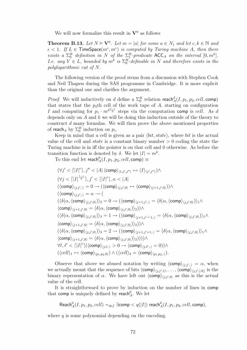
We will now formalize this result in V0 as follows

Theorem B.13. Let N V0. Let m = |a| for some a ∈ N1 and let c, k ∈ N andǫ < 1. If L ∈ TimeSpace(mc,mǫ) is computed by Turing machine A, then thereexists a ΣB

0 definition in N of the ΣB1 -predicate ACCA on the interval [0,mk].

I.e. any Y ∈ L, bounded by mk is ΣB0 -definable in N and therefore exists in the

polylogarithmic cut of N .

The following version of the proof stems from a discussion with Stephen Cookand Neil Thapen during the SAS programme in Cambridge. It is more explicitthan the original one and clarifies the argument.

Proof. We will inductively on d define a ΣB0 relation reachd

A(I, p1, p2, cell, comp)that states that the p2th cell of the work tape of A, starting on configurationI and computing for p1 · md 1−ǫ

k steps via the computation comp is cell. As ddepends only on A and k we will be doing this induction outside of the theory toconstruct d many formulas. We will then prove the above mentioned propertiesof reachA by ΣB

0 induction on p1.Keep in mind that a cell is given as a pair 〈bit, state〉, where bit is the actual

value of the cell and state is a constant binary number > 0 coding the state theTuring machine is in iff the pointer is on that cell and 0 otherwise. As before thetransition function is denoted by δ. We let |I| = mk.

To this end let reach0A(I, p1, p2, cell, comp) ≡

(∀j′ < ⌈|I|ǫ⌉, j′′ < |A| 〈comp〉〈1,j′,j′′〉 ↔ 〈I〉〈j′,j′′〉)∧(∀j < ⌈|I| 1−ǫ

k ⌉, j′ < ⌈|I|ǫ⌉, α < |A|(〈comp〉〈j,j′,·〉 = 0→ (〈comp〉〈j,j′,0〉 ↔ 〈comp〉〈j+1,j′,0〉))∧(〈comp〉〈j,j′,·〉 = α→ (

(〈δ(α, 〈comp〉〈j,j′,0〉)〉3 = 0→ (〈comp〉〈j+1,j′,·〉 = 〈δ(α, 〈comp〉〈j,j′,0〉)〉1∧〈comp〉〈j+1,j′,0〉 = 〈δ(α, 〈comp〉〈j,j′,0〉)〉2))∧(〈δ(α, 〈comp〉〈j,j′,0〉)〉3 = 1→ (〈comp〉〈j+1,j′

·−1,·〉 = 〈δ(α, 〈comp〉〈j,j′,0〉)〉1∧〈comp〉〈j+1,j′,0〉 = 〈δ(α, 〈comp〉〈j,j′,0〉)〉2))∧(〈δ(α, 〈comp〉〈j,j′,0〉)〉3 = 2→ (〈comp〉〈j+1,j′+1,·〉 = 〈δ(α, 〈comp〉〈j,j′,0〉)〉1∧〈comp〉〈j+1,j′,0〉 = 〈δ(α, 〈comp〉〈j,j′,0〉)〉2))))∧∀ℓ, ℓ′ < ⌈|I|ǫ⌉(〈comp〉〈j,ℓ,·〉 > 0→ 〈comp〉〈j,ℓ′,·〉 = 0))∧(〈cell〉1 ↔ 〈comp〉〈p1,p2,0〉) ∧ (〈cell〉2 = 〈comp〉〈p1,p2,·〉).

Observe that above we abused notation by writing 〈comp〉〈j,j′,·〉 = α, whenwe actually meant that the sequence of bits 〈comp〉〈j,j′,1〉, . . . , 〈comp〉〈j,j′,|A|〉 is thebinary representation of α. We have left out 〈comp〉〈j,j′,0〉 as this is the actualvalue of the cell.

It is straightforward to prove by induction on the number of lines in comp

that comp is uniquely defined by reach0A. We let

Reach0A(I, p1, p2, cell) =def ∃comp < q(|I|) reach0

A(I, p1, p2, cell, comp),

where q is some polynomial depending on the encoding.

72

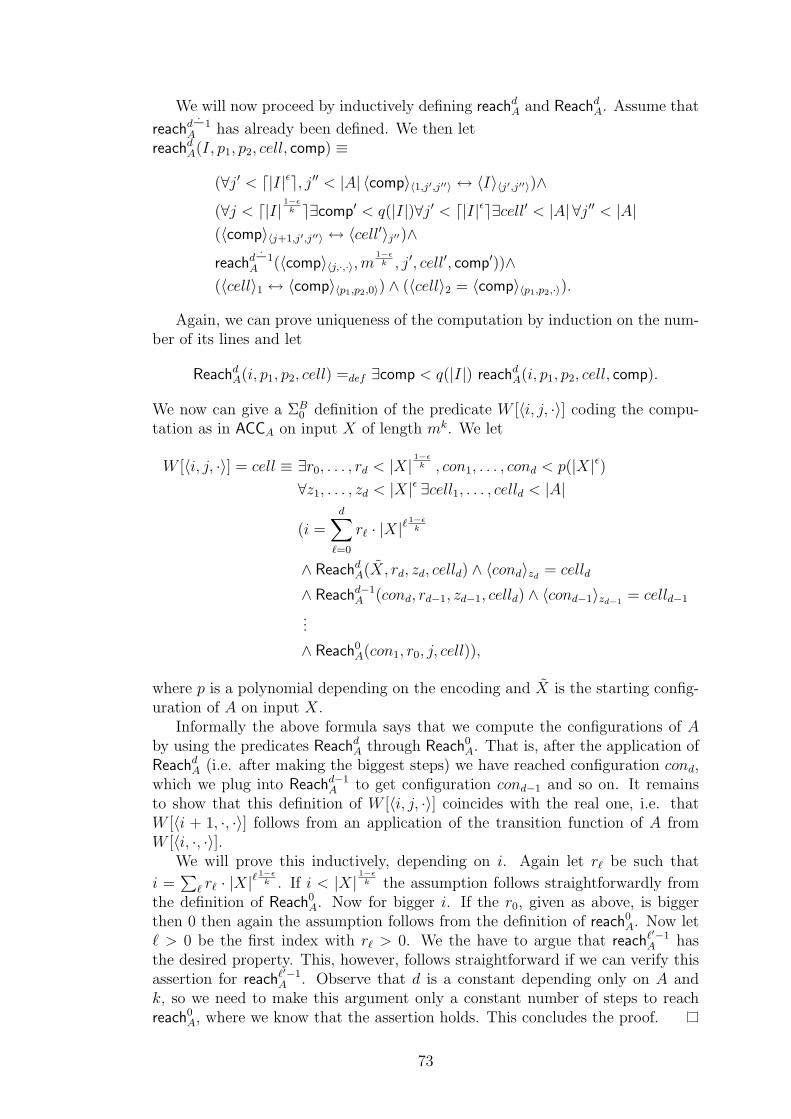
We will now proceed by inductively defining reachdA and Reachd

A. Assume that

reachd·−1

A has already been defined. We then letreachd

A(I, p1, p2, cell, comp) ≡

(∀j′ < ⌈|I|ǫ⌉, j′′ < |A| 〈comp〉〈1,j′,j′′〉 ↔ 〈I〉〈j′,j′′〉)∧(∀j < ⌈|I| 1−ǫ

k ⌉∃comp′ < q(|I|)∀j′ < ⌈|I|ǫ⌉∃cell′ < |A| ∀j′′ < |A|(〈comp〉〈j+1,j′,j′′〉 ↔ 〈cell′〉j′′)∧reachd

·−1A (〈comp〉〈j,·,·〉,m

1−ǫk , j′, cell′, comp′))∧

(〈cell〉1 ↔ 〈comp〉〈p1,p2,0〉) ∧ (〈cell〉2 = 〈comp〉〈p1,p2,·〉).

Again, we can prove uniqueness of the computation by induction on the num-ber of its lines and let

ReachdA(i, p1, p2, cell) =def ∃comp < q(|I|) reachd

A(i, p1, p2, cell, comp).

We now can give a ΣB0 definition of the predicate W [〈i, j, ·〉] coding the compu-

tation as in ACCA on input X of length mk. We let

W [〈i, j, ·〉] = cell ≡ ∃r0, . . . , rd < |X|1−ǫ

k , con1, . . . , cond < p(|X|ǫ)∀z1, . . . , zd < |X|ǫ ∃cell1, . . . , celld < |A|

(i =d∑

ℓ=0

rℓ · |X|ℓ1−ǫ

k

∧ ReachdA(X, rd, zd, celld) ∧ 〈cond〉zd

= celld

∧ Reachd−1A (cond, rd−1, zd−1, celld) ∧ 〈cond−1〉zd−1

= celld−1

...

∧ Reach0A(con1, r0, j, cell)),

where p is a polynomial depending on the encoding and X is the starting config-uration of A on input X.

Informally the above formula says that we compute the configurations of Aby using the predicates Reachd

A through Reach0A. That is, after the application of

ReachdA (i.e. after making the biggest steps) we have reached configuration cond,

which we plug into Reachd−1A to get configuration cond−1 and so on. It remains

to show that this definition of W [〈i, j, ·〉] coincides with the real one, i.e. thatW [〈i + 1, ·, ·〉] follows from an application of the transition function of A fromW [〈i, ·, ·〉].

We will prove this inductively, depending on i. Again let rℓ be such that

i =∑

ℓ rℓ · |X|ℓ1−ǫ

k . If i < |X| 1−ǫk the assumption follows straightforwardly from

the definition of Reach0A. Now for bigger i. If the r0, given as above, is bigger

then 0 then again the assumption follows from the definition of reach0A. Now let

ℓ > 0 be the first index with rℓ > 0. We the have to argue that reachℓ′−1A has

the desired property. This, however, follows straightforward if we can verify thisassertion for reachℓ′−1

A . Observe that d is a constant depending only on A andk, so we need to make this argument only a constant number of steps to reachreach0

A, where we know that the assertion holds. This concludes the proof.

73

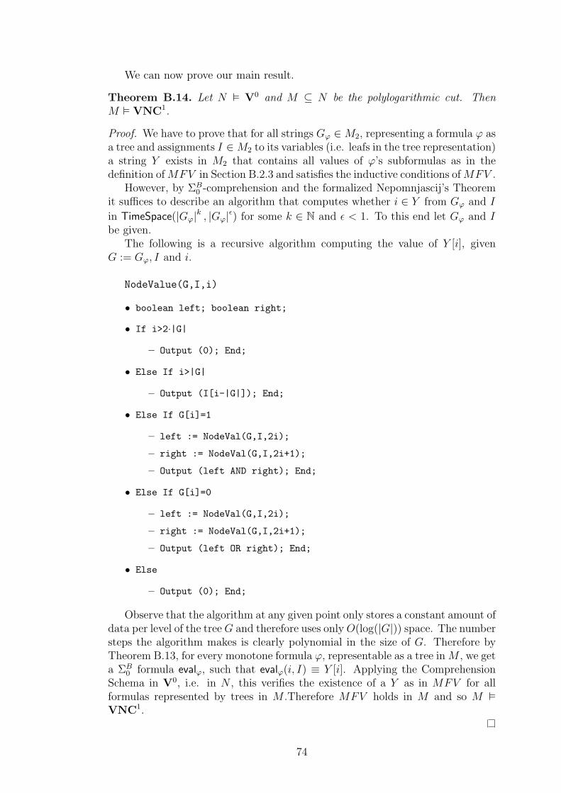
We can now prove our main result.

Theorem B.14. Let N V0 and M ⊆ N be the polylogarithmic cut. ThenM VNC1.

Proof. We have to prove that for all strings Gϕ ∈M2, representing a formula ϕ asa tree and assignments I ∈M2 to its variables (i.e. leafs in the tree representation)a string Y exists in M2 that contains all values of ϕ’s subformulas as in thedefinition ofMFV in Section B.2.3 and satisfies the inductive conditions ofMFV .

However, by ΣB0 -comprehension and the formalized Nepomnjascij’s Theorem

it suffices to describe an algorithm that computes whether i ∈ Y from Gϕ and I

in TimeSpace(|Gϕ|k , |Gϕ|ǫ) for some k ∈ N and ǫ < 1. To this end let Gϕ and Ibe given.

The following is a recursive algorithm computing the value of Y [i], givenG := Gϕ, I and i.

NodeValue(G,I,i)

• boolean left; boolean right;

• If i>2·|G|

– Output (0); End;

• Else If i>|G|

– Output (I[i-|G|]); End;

• Else If G[i]=1

– left := NodeVal(G,I,2i);

– right := NodeVal(G,I,2i+1);

– Output (left AND right); End;

• Else If G[i]=0

– left := NodeVal(G,I,2i);

– right := NodeVal(G,I,2i+1);

– Output (left OR right); End;

• Else

– Output (0); End;

Observe that the algorithm at any given point only stores a constant amount ofdata per level of the treeG and therefore uses onlyO(log(|G|)) space. The numbersteps the algorithm makes is clearly polynomial in the size of G. Therefore byTheorem B.13, for every monotone formula ϕ, representable as a tree inM , we geta ΣB

0 formula evalϕ, such that evalϕ(i, I) ≡ Y [i]. Applying the ComprehensionSchema in V0, i.e. in N , this verifies the existence of a Y as in MFV for allformulas represented by trees in M .Therefore MFV holds in M and so M

VNC1.

74

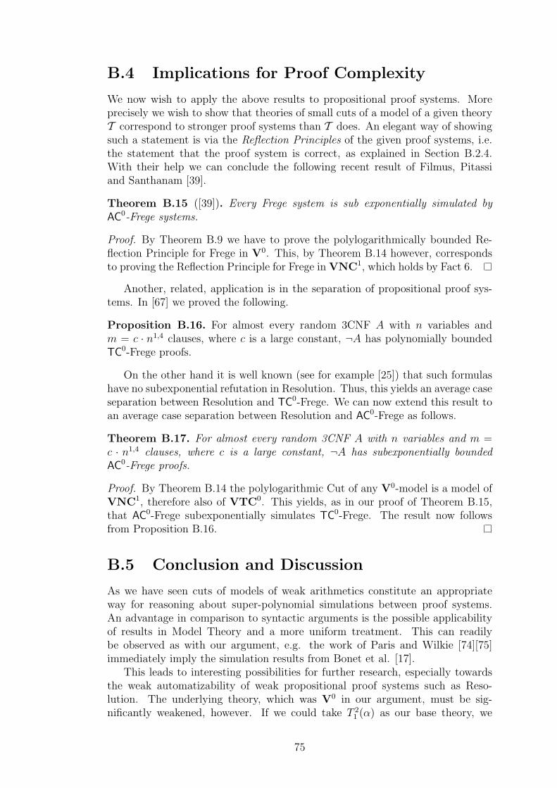
B.4 Implications for Proof Complexity

We now wish to apply the above results to propositional proof systems. Moreprecisely we wish to show that theories of small cuts of a model of a given theoryT correspond to stronger proof systems than T does. An elegant way of showingsuch a statement is via the Reflection Principles of the given proof systems, i.e.the statement that the proof system is correct, as explained in Section B.2.4.With their help we can conclude the following recent result of Filmus, Pitassiand Santhanam [39].

Theorem B.15 ([39]). Every Frege system is sub exponentially simulated byAC0-Frege systems.

Proof. By Theorem B.9 we have to prove the polylogarithmically bounded Re-flection Principle for Frege in V0. This, by Theorem B.14 however, correspondsto proving the Reflection Principle for Frege in VNC1, which holds by Fact 6.

Another, related, application is in the separation of propositional proof sys-tems. In [67] we proved the following.

Proposition B.16. For almost every random 3CNF A with n variables andm = c · n1,4 clauses, where c is a large constant, ¬A has polynomially boundedTC0-Frege proofs.

On the other hand it is well known (see for example [25]) that such formulashave no subexponential refutation in Resolution. Thus, this yields an average caseseparation between Resolution and TC0-Frege. We can now extend this result toan average case separation between Resolution and AC0-Frege as follows.

Theorem B.17. For almost every random 3CNF A with n variables and m =c · n1,4 clauses, where c is a large constant, ¬A has subexponentially boundedAC0-Frege proofs.

Proof. By Theorem B.14 the polylogarithmic Cut of any V0-model is a model ofVNC1, therefore also of VTC0. This yields, as in our proof of Theorem B.15,that AC0-Frege subexponentially simulates TC0-Frege. The result now followsfrom Proposition B.16.

B.5 Conclusion and Discussion

As we have seen cuts of models of weak arithmetics constitute an appropriateway for reasoning about super-polynomial simulations between proof systems.An advantage in comparison to syntactic arguments is the possible applicabilityof results in Model Theory and a more uniform treatment. This can readilybe observed as with our argument, e.g. the work of Paris and Wilkie [74][75]immediately imply the simulation results from Bonet et al. [17].

This leads to interesting possibilities for further research, especially towardsthe weak automatizability of weak propositional proof systems such as Reso-lution. The underlying theory, which was V0 in our argument, must be sig-nificantly weakened, however. If we could take T 2

1 (α) as our base theory, we

75

could reason about whether Res(log) has the feasible interpolation property inthe same way as Krajıcek and Pudlak [61], Bonet, Pitassi and Raz [18] or Bonet,Domingo, Gavalda, Maciel, and Pitassi [17]. Now, if Res(log) does not have quasi-polynomial feasible interpolation we know by a result from Atserias and Bonet [6]that Resolution is not weakly automatizable, so we would be finished. Whetherwe can actually do it depends on the strength of the theory the polylogarithmiccut of T 2

1 (α) models and if we can formalize some sort of iterated multiplication(such as in [51]) in that theory. Also, the security of Diffie-Hellman seems to bea more appropriate assumption than that of RSA, as the computational powerneeded to verify the correctness of Diffie-Hellman seems to be lower.

B.6 Acknowledgements

I want to thank Steve Cook, Jan Krajıcek and Neil Thapen for helpful suggestionsand discussion, Emil Jerabek for his comments and for answering my questionsand the participants of the MALOA Special Semester in Proof Complexity inPrague 2011 for enduring a sloppy and sometimes faulty exposition of this proofand still coming up with helpful comments. I also want to thank the anonymousreferees for pointing out various mistakes and for giving interesting suggestions.

76

C. Necessary Background

Here we will summarize and briefly explain the logical and complexity theoreticconcepts we need.

C.1 Logical Preliminaries

Historically, logic started to become more influential in mathematics with theadvent of methods which are not ”obviously true”. At latest from the 19thcentury on mathematical arguments became more abstract and in many casesused objects which were not rigorously constructed. A famous early example isDirichlet’s definition of a function that is 1 on the rational and 0 on the irrationalnumbers. This was revolutionary at its time as its definition did not provide aclear means of computing the image. Aside from leading to various new results,use of such methods also bore a great risk of inconsistency. This let to variouscriticisms of such arguments as to whether these results should be acceptable atall. David Hilbert, one of the strongest proponents of the use of such non-finitarytechniques, tried to counter such criticism in his famous Conservation Program:To eliminate the above problem, can we give an explicit collection of feasible truestatements and a system of rules, which allows us to manipulate sentences in away that does not alter the truth value of true sentences, such that all statementsabout finitary objects proved in an abstract way can be reproved using thatsystem? Hilbert himself believed that a fragment of elementary number theoryexists that would be appropriate as a base for an axiomatization. This fragmentshould be consisting of ”gewisse außerlogische diskrete Objekte, die anschaulichals unmittelbares Erlebnis vor allem Denken da sind. Soll das logische Schließensicher sein, so mussen sich diese Objekte vollkommen in allen Teilen uberblickenlassen und ihre Aufweisung, ihre Unterscheidung, ihr Aufeinanderfolgen ist mitden Objekten zugleich unmittelbar anschaulich fur uns da als etwas, das sichnicht noch auf etwas anderes reduzieren laßt.”1 [52]. That this view is not correctwas shown shortly after by Kurt Godel as we will see in a moment.

Hilbert’s program became the driving force of introducing a rigorous logicalframework into mathematics. Although its original goal proved to be impossibleto achieve, it became extremely successful in analyzing and structuring mathe-matics.

For now, we will call such a system of deduction a calculus and such an explicitcollection of statements a theory. To treat the above question we need to talkabout objects that live in a mathematical world, e.g. the elements of the set ofnatural numbers. We will, however, start with easier objects to cope with. Thatis, we will start with statements as primitives and ways to reason about them.An excellent and more extensive survey can be found in [22] or with a differentfocus in [35].

1”extra-logical discrete objects, which exist intuitively as immediate experience before allthought. If logical inference is to be certain, then these objects must be capable of beingcompletely surveyed in all their parts, and their presentation, their difference, their succession(like the objects themselves) must exist for us immediately, intuitively, as something whichcannot be reduced to something else.”

77

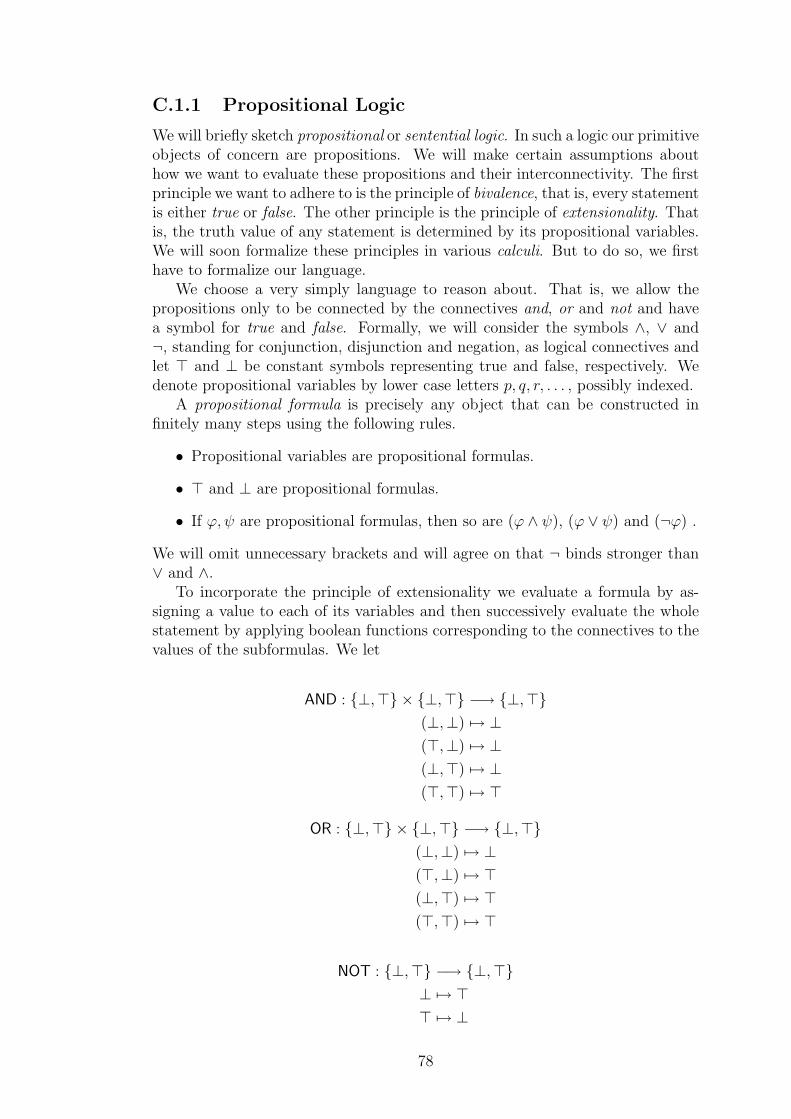
C.1.1 Propositional Logic

We will briefly sketch propositional or sentential logic. In such a logic our primitiveobjects of concern are propositions. We will make certain assumptions abouthow we want to evaluate these propositions and their interconnectivity. The firstprinciple we want to adhere to is the principle of bivalence, that is, every statementis either true or false. The other principle is the principle of extensionality. Thatis, the truth value of any statement is determined by its propositional variables.We will soon formalize these principles in various calculi. But to do so, we firsthave to formalize our language.

We choose a very simply language to reason about. That is, we allow thepropositions only to be connected by the connectives and, or and not and havea symbol for true and false. Formally, we will consider the symbols ∧, ∨ and¬, standing for conjunction, disjunction and negation, as logical connectives andlet ⊤ and ⊥ be constant symbols representing true and false, respectively. Wedenote propositional variables by lower case letters p, q, r, . . . , possibly indexed.

A propositional formula is precisely any object that can be constructed infinitely many steps using the following rules.

• Propositional variables are propositional formulas.

• ⊤ and ⊥ are propositional formulas.

• If ϕ, ψ are propositional formulas, then so are (ϕ ∧ ψ), (ϕ ∨ ψ) and (¬ϕ) .

We will omit unnecessary brackets and will agree on that ¬ binds stronger than∨ and ∧.

To incorporate the principle of extensionality we evaluate a formula by as-signing a value to each of its variables and then successively evaluate the wholestatement by applying boolean functions corresponding to the connectives to thevalues of the subformulas. We let

AND : ⊥,⊤ × ⊥,⊤ −→ ⊥,⊤(⊥,⊥) 7→ ⊥(⊤,⊥) 7→ ⊥(⊥,⊤) 7→ ⊥(⊤,⊤) 7→ ⊤

OR : ⊥,⊤ × ⊥,⊤ −→ ⊥,⊤(⊥,⊥) 7→ ⊥(⊤,⊥) 7→ ⊤(⊥,⊤) 7→ ⊤(⊤,⊤) 7→ ⊤

NOT : ⊥,⊤ −→ ⊥,⊤⊥ 7→ ⊤⊤ 7→ ⊥

78

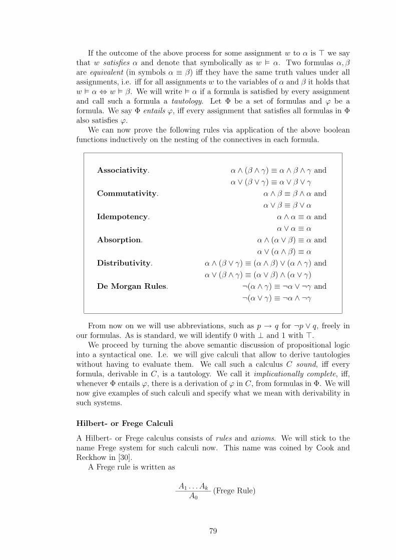
If the outcome of the above process for some assignment w to α is ⊤ we saythat w satisfies α and denote that symbolically as w α. Two formulas α, βare equivalent (in symbols α ≡ β) iff they have the same truth values under allassignments, i.e. iff for all assignments w to the variables of α and β it holds thatw α ⇔ w β. We will write α if a formula is satisfied by every assignmentand call such a formula a tautology. Let Φ be a set of formulas and ϕ be aformula. We say Φ entails ϕ, iff every assignment that satisfies all formulas in Φalso satisfies ϕ.

We can now prove the following rules via application of the above booleanfunctions inductively on the nesting of the connectives in each formula.

Associativity. α ∧ (β ∧ γ) ≡ α ∧ β ∧ γ and

α ∨ (β ∨ γ) ≡ α ∨ β ∨ γCommutativity. α ∧ β ≡ β ∧ α and

α ∨ β ≡ β ∨ αIdempotency. α ∧ α ≡ α and

α ∨ α ≡ α

Absorption. α ∧ (α ∨ β) ≡ α and

α ∨ (α ∧ β) ≡ α

Distributivity. α ∧ (β ∨ γ) ≡ (α ∧ β) ∨ (α ∧ γ) and

α ∨ (β ∧ γ) ≡ (α ∨ β) ∧ (α ∨ γ)De Morgan Rules. ¬(α ∧ γ) ≡ ¬α ∨ ¬γ and

¬(α ∨ γ) ≡ ¬α ∧ ¬γ

From now on we will use abbreviations, such as p → q for ¬p ∨ q, freely inour formulas. As is standard, we will identify 0 with ⊥ and 1 with ⊤.

We proceed by turning the above semantic discussion of propositional logicinto a syntactical one. I.e. we will give calculi that allow to derive tautologieswithout having to evaluate them. We call such a calculus C sound, iff everyformula, derivable in C, is a tautology. We call it implicationally complete, iff,whenever Φ entails ϕ, there is a derivation of ϕ in C, from formulas in Φ. We willnow give examples of such calculi and specify what we mean with derivability insuch systems.

Hilbert- or Frege Calculi

A Hilbert- or Frege calculus consists of rules and axioms. We will stick to thename Frege system for such calculi now. This name was coined by Cook andReckhow in [30].

A Frege rule is written as

A1 . . . Ak (Frege Rule)A0

79

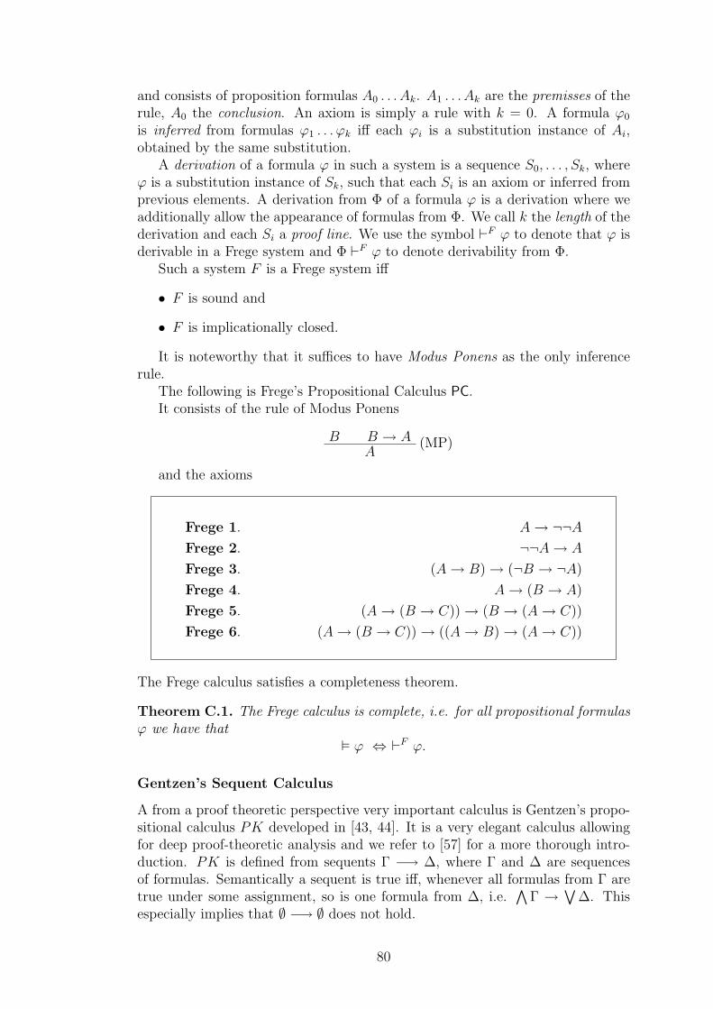
and consists of proposition formulas A0 . . . Ak. A1 . . . Ak are the premisses of therule, A0 the conclusion. An axiom is simply a rule with k = 0. A formula ϕ0

is inferred from formulas ϕ1 . . . ϕk iff each ϕi is a substitution instance of Ai,obtained by the same substitution.

A derivation of a formula ϕ in such a system is a sequence S0, . . . , Sk, whereϕ is a substitution instance of Sk, such that each Si is an axiom or inferred fromprevious elements. A derivation from Φ of a formula ϕ is a derivation where weadditionally allow the appearance of formulas from Φ. We call k the length of thederivation and each Si a proof line. We use the symbol ⊢F ϕ to denote that ϕ isderivable in a Frege system and Φ ⊢F ϕ to denote derivability from Φ.

Such a system F is a Frege system iff

• F is sound and

• F is implicationally closed.

It is noteworthy that it suffices to have Modus Ponens as the only inferencerule.

The following is Frege’s Propositional Calculus PC.It consists of the rule of Modus Ponens

B B → A (MP)A

and the axioms

Frege 1. A→ ¬¬AFrege 2. ¬¬A→ A

Frege 3. (A→ B)→ (¬B → ¬A)

Frege 4. A→ (B → A)

Frege 5. (A→ (B → C))→ (B → (A→ C))

Frege 6. (A→ (B → C))→ ((A→ B)→ (A→ C))

The Frege calculus satisfies a completeness theorem.

Theorem C.1. The Frege calculus is complete, i.e. for all propositional formulasϕ we have that

ϕ ⇔ ⊢F ϕ.

Gentzen’s Sequent Calculus

A from a proof theoretic perspective very important calculus is Gentzen’s propo-sitional calculus PK developed in [43, 44]. It is a very elegant calculus allowingfor deep proof-theoretic analysis and we refer to [57] for a more thorough intro-duction. PK is defined from sequents Γ −→ ∆, where Γ and ∆ are sequencesof formulas. Semantically a sequent is true iff, whenever all formulas from Γ aretrue under some assignment, so is one formula from ∆, i.e.

∧Γ → ∨

∆. Thisespecially implies that ∅ −→ ∅ does not hold.

80

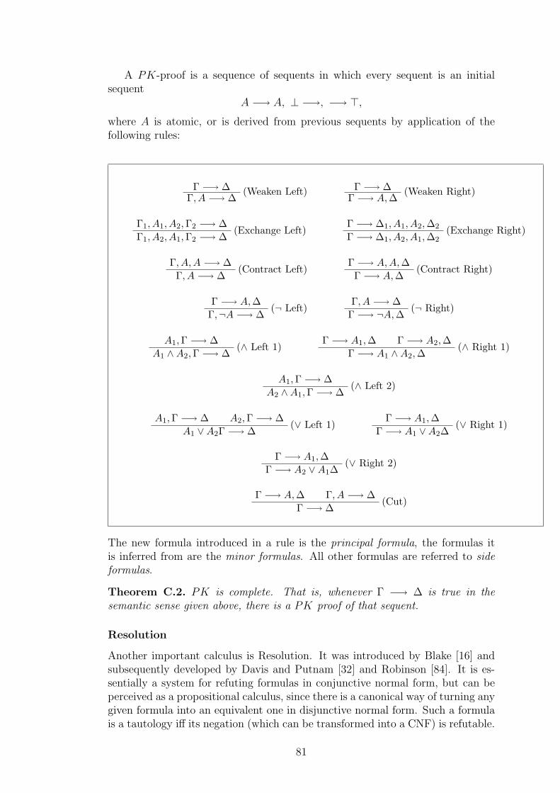
A PK-proof is a sequence of sequents in which every sequent is an initialsequent

A −→ A, ⊥ −→, −→ ⊤,where A is atomic, or is derived from previous sequents by application of thefollowing rules:

Γ −→ ∆ (Weaken Left)Γ, A −→ ∆

Γ −→ ∆ (Weaken Right)Γ −→ A,∆

Γ1, A1, A2,Γ2 −→ ∆(Exchange Left)

Γ1, A2, A1,Γ2 −→ ∆

Γ −→ ∆1, A1, A2,∆2 (Exchange Right)Γ −→ ∆1, A2, A1,∆2

Γ, A,A −→ ∆(Contract Left)

Γ, A −→ ∆

Γ −→ A,A,∆(Contract Right)

Γ −→ A,∆

Γ −→ A,∆(¬ Left)

Γ,¬A −→ ∆

Γ, A −→ ∆(¬ Right)

Γ −→ ¬A,∆

A1,Γ −→ ∆(∧ Left 1)

A1 ∧A2,Γ −→ ∆

Γ −→ A1,∆ Γ −→ A2,∆ (∧ Right 1)Γ −→ A1 ∧A2,∆

A1,Γ −→ ∆(∧ Left 2)

A2 ∧A1,Γ −→ ∆

A1,Γ −→ ∆ A2,Γ −→ ∆(∨ Left 1)

A1 ∨A2Γ −→ ∆

Γ −→ A1,∆ (∨ Right 1)Γ −→ A1 ∨A2∆

Γ −→ A1,∆ (∨ Right 2)Γ −→ A2 ∨A1∆

Γ −→ A,∆ Γ, A −→ ∆(Cut)

Γ −→ ∆

The new formula introduced in a rule is the principal formula, the formulas itis inferred from are the minor formulas. All other formulas are referred to sideformulas.

Theorem C.2. PK is complete. That is, whenever Γ −→ ∆ is true in thesemantic sense given above, there is a PK proof of that sequent.

Resolution

Another important calculus is Resolution. It was introduced by Blake [16] andsubsequently developed by Davis and Putnam [32] and Robinson [84]. It is es-sentially a system for refuting formulas in conjunctive normal form, but can beperceived as a propositional calculus, since there is a canonical way of turning anygiven formula into an equivalent one in disjunctive normal form. Such a formulais a tautology iff its negation (which can be transformed into a CNF) is refutable.

81

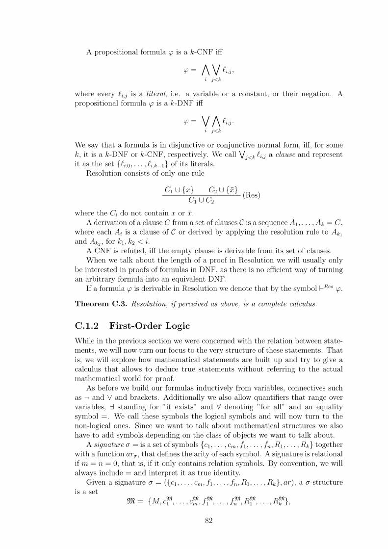
A propositional formula ϕ is a k-CNF iff

ϕ =∧

i

∨

j<k

ℓi,j,

where every ℓi,j is a literal, i.e. a variable or a constant, or their negation. Apropositional formula ϕ is a k-DNF iff

ϕ =∨

i

∧

j<k

ℓi,j.

We say that a formula is in disjunctive or conjunctive normal form, iff, for somek, it is a k-DNF or k-CNF, respectively. We call

∨j<k ℓi,j a clause and represent

it as the set ℓi,0, . . . , ℓi,k−1 of its literals.Resolution consists of only one rule

C1 ∪ x C2 ∪ x(Res)

C1 ∪ C2

where the Ci do not contain x or x.A derivation of a clause C from a set of clauses C is a sequence A1, . . . , Ak = C,

where each Ai is a clause of C or derived by applying the resolution rule to Ak1

and Ak2 , for k1, k2 < i.A CNF is refuted, iff the empty clause is derivable from its set of clauses.When we talk about the length of a proof in Resolution we will usually only

be interested in proofs of formulas in DNF, as there is no efficient way of turningan arbitrary formula into an equivalent DNF.

If a formula ϕ is derivable in Resolution we denote that by the symbol ⊢Res ϕ.

Theorem C.3. Resolution, if perceived as above, is a complete calculus.

C.1.2 First-Order Logic

While in the previous section we were concerned with the relation between state-ments, we will now turn our focus to the very structure of these statements. Thatis, we will explore how mathematical statements are built up and try to give acalculus that allows to deduce true statements without referring to the actualmathematical world for proof.

As before we build our formulas inductively from variables, connectives suchas ¬ and ∨ and brackets. Additionally we also allow quantifiers that range overvariables, ∃ standing for ”it exists” and ∀ denoting ”for all” and an equalitysymbol =. We call these symbols the logical symbols and will now turn to thenon-logical ones. Since we want to talk about mathematical structures we alsohave to add symbols depending on the class of objects we want to talk about.

A signature σ = is a set of symbols c1, . . . , cm, f1, . . . , fn, R1, . . . , Rk togetherwith a function arσ, that defines the arity of each symbol. A signature is relationalif m = n = 0, that is, if it only contains relation symbols. By convention, we willalways include = and interpret it as true identity.

Given a signature σ = (c1, . . . , cm, f1, . . . , fn, R1, . . . , Rk, ar), a σ-structureis a set

M = M, cM1 , . . . , cM

m , fM

1 , . . . , fM

n , RM

1 , . . . , RM

k ,

82

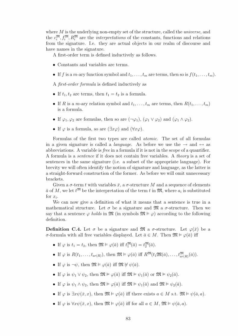
whereM is the underlying non-empty set of the structure, called the universe, andthe cMi , f

M

i , RM

i are the interpretations of the constants, functions and relationsfrom the signature. I.e. they are actual objects in our realm of discourse andhave names in the signature.

A first-order term is defined inductively as follows.

• Constants and variables are terms.

• If f is am-ary function symbol and t1, . . . , tm are terms, then so is f(t1, . . . , tm).

A first-order formula is defined inductively as

• If t1, t2 are terms, then t1 = t2 is a formula.

• If R is a m-ary relation symbol and t1, . . . , tm are terms, then R(t1, . . . , tm)is a formula.

• If ϕ1, ϕ2 are formulas, then so are (¬ϕ1), (ϕ1 ∨ ϕ2) and (ϕ1 ∧ ϕ2).

• If ϕ is a formula, so are (∃xϕ) and (∀xϕ).

Formulas of the first two types are called atomic. The set of all formulasin a given signature is called a language. As before we use the → and ↔ asabbreviations. A variable is free in a formula if it is not in the scope of a quantifier.A formula is a sentence if it does not contain free variables. A theory is a set ofsentences in the same signature (i.e. a subset of the appropriate language). Forbrevity we will often identify the notion of signature and language, as the latter isa straight-forward construction of the former. As before we will omit unnecessarybrackets.

Given a σ-term t with variables x, a σ-structure M and a sequence of elementsa of M , we let tM be the interpretation of the term t in M, where ai is substitutedfor xi.

We can now give a definition of what it means that a sentence is true in amathematical structure. Let σ be a signature and M a σ-structure. Then wesay that a sentence ϕ holds in M (in symbols M ϕ) according to the followingdefinition.

Definition C.4. Let σ be a signature and M a σ-structure. Let ϕ(x) be aσ-formula with all free variables displayed. Let a ∈M . Then M ϕ(a) iff

• If ϕ is t1 = t2, then M ϕ(a) iff tM1 (a) = tM2 (a).

• If ϕ is R(t1, . . . , tar(R)), then M ϕ(a) iff RM(t1M(a), . . . , tMar(R)(a)).

• If ϕ is ¬ψ, then M ϕ(a) iff M 6 ψ(a).

• If ϕ is ψ1 ∨ ψ2, then M ϕ(a) iff M ψ1(a) or M ψ2(a).

• If ϕ is ψ1 ∧ ψ2, then M ϕ(a) iff M ψ1(a) and M ψ2(a).

• If ϕ is ∃xψ(x, x), then M ϕ(a) iff there exists a ∈M s.t. M ψ(a, a).

• If ϕ is ∀xψ(x, x), then M ϕ(a) iff for all a ∈M , M ψ(a, a).

83

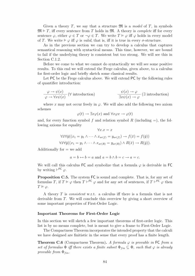
Given a theory T , we say that a structure M is a model of T , in symbolsM T , iff every sentence from T holds in M. A theory is complete iff for everysentence ϕ, either ϕ ∈ T or ¬ϕ ∈ T . We write T ϕ iff ϕ holds in every modelof T . We write ϕ iff ϕ is valid, that is, iff it is true in every σ-structure.

As in the previous section we can try to develop a calculus that capturessemantical reasoning with syntactical means. This time, however, we are boundto fail if the underlying theory is consistent but too strong. We will see this inSection C.1.2.

Before we come to what we cannot do syntactically we will see some positiveresults. To this end we will extend the Frege calculus, given above, to a calculusfor first-order logic and briefly sketch some classical results.

Let PC be the Frege calculus above. We will extend PC by the following rulesof quantifier introduction:

ϕ→ ψ(x)(∀ introduction)

ϕ→ ∀xψ(x)

ψ(x)→ ϕ(∃ introduction)∃xψ(x)→ ϕ

where x may not occur freely in ϕ. We will also add the following two axiomschemes

ϕ(t)→ ∃xϕ(x) and ∀xϕx→ ϕ(t)

and, for every function symbol f and relation symbol R (including =), the fol-lowing axioms for equality

∀x.x = x

∀x∀y((x1 = y1 ∧ · · · ∧ xar(f) = yar(f))→ f(x) = f(y))

∀x∀y((x1 = y1 ∧ · · · ∧ xar(R) = yar(R)) ∧R(x)→ R(y)).

Additionally for = we add

a = b↔ b = a and a = b ∧ b = c→ a = c.

We will call this calculus FC and symbolize that a formula ϕ is derivable in FC

by writing ⊢FC ϕ.

Proposition C.5. The system FC is sound and complete. That is, for any set offormulas T , if T ϕ then T ⊢FC ϕ and for any set of sentences, if T ⊢FC ϕ thenT ϕ.

A theory T is consistent w.r.t. a calculus iff there is a formula that is notderivable from T . We will conclude this overview by giving a short overview ofsome important properties of First-Order Logic.

Important Theorems for First-Order Logic

In this section we will sketch a few important theorems of first-order logic. Thislist is by no means complete, but is meant to give a frame to First-Order Logic.

The Compactness Theorem incorporates the intended property that the calculiwe have designed are finitistic in the sense that every proof has a finite length.

Theorem C.6 (Compactness Theorem). A formula ϕ is provable in FC from aset of formulas Φ iff there exists a finite subset Φfin ⊆ Φ, such that ϕ is alreadyprovable from Φfin.

84

From a (first-order) logical perspective, the notion of size of an arbitrarymodel is not well definable, when we take a look at infinite structures. This isexemplified in the Lowenheim-Skolem Theorem.

Theorem C.7 (Lowenheim-Skolem). Let L be some first-order language and letΦ be a set of L-formulas that is satisfiable over an infinite universe, with κ = |L|.Then there is an L-structure M of cardinality max(κ,ℵ0) that satisfies Φ.

We now turn to the theorems that obliterated Hilbert’s vision of being ableto turn every ideal proof into a finitistic one. Godel’s Incompleteness Theorems[45] show that there is no formal system that admits on the one hand a decidablenotion of provability and on the other hand is complete in the sense that it canprove every Π1 statement that holds in the natural numbers.

Numerous books have been written about the Incompleteness Theorems, so wewill only state the theorems. We refer a more interested reader to the literature,for example [8], [22] or [80].

We will first give Godel’s original version of his first theorem and then Rosser’sversion, which does not need the additional assumption of ω-consistency. A theoryT is called ω-consistent iff it is consistent in a way with the natural numbers.That is, if an existential statement ∃ϕ(x) is provable from T , then there must bea numeral n such that T does not prove ¬ϕ(n).

Theorem C.8 (Godel’s First Incompleteness Theorem). Let T be a consistent,recursive theory extending Robinson Arithmetic. Then there is a true sentence ϕ,such that ϕ is not provable from T . Moreover, if T is ω consistent, then ¬ϕ isalso not provable from T .

Here, the formula ϕ is explicitly constructed from T and basically asserts itsown unprovability from T , i.e. it is an encoding of the statement ”I am notprovable in T”. Rosser [85] subsequently weakened the assumptions of Godel’sTheorem.

Theorem C.9 (Rosser’s Theorem). There is no consistent, recursive and com-plete theory extending Robinson Arithmetic.

Soon after publishing his First Incompleteness Theorem, Godel became awareof the existence of another example example of a statement that is not provablein T .

Theorem C.10 (Godel’s Second Incompleteness Theorem). There is no con-sistent, recursive theory extending Robinson Arithmetic that can prove its ownconsistency.

The proof of Theorem C.10 actually shows that the consistency statement isequivalent to the sentence from Theorem C.8 asserting its own unprovability.

C.2 Complexity Theory

Godel’s Incompleteness Theorems imply that there are problems that cannotbe solved algorithmically. In Complexity Theory we are concerned with thoseproblems that can be. Even if problems are solvable they differ in various aspects,

85

such as time and space needed for the computation. To make these notions precisewe first need to define what our model of computation should be. We will use aTuring machine as our principal model of computation.

Definition C.11. A deterministic Turing machine is defined by a tuple (K,Σ, δ, s),where K is a set of states containing the initial state s, Σ a set of symbols, con-taining (the ”first” symbol) and ⊔ (the ”blank” symbol), and δ : K × Σ −→K ∪ ”halt”, ”yes”, ”no” × Σ × ←,→, ↓ the transition function. The state”halt” is called the halting state, the state ”yes” the accepting state and the state”no” the rejecting state.

We view a Turing machine as a means of computation in the following sense.The machine works on a to the right infinite work tape consisting of cells, each ofwhich can be filled with symbols from Σ. It has one read/write head which pointsto a cell. Initially the tape contains only the input x ∈ Σ∗ on its leftmost cells and⊔ on the others. The read/write head points to the leftmost cell and the machineis in its initial state s. A Turing machine computation is a sequence of applicationsof the transition function until the machine is in one of the states ”halt”, ”yes”or ”no”. The transition function is applied as follows. If the read/write headpoints to cell i, the machine is in state t and the cell contains symbol y ∈ Σ, thenthe machine looks at δ(t, y) = (t′, y′, dir) and replaces y on cell i by y′, movesin direction dir, that is if dir =← it points to cell i ·− 1, if dir =→ it points tocell i + 1 and if dir =↓ it points to cell i, and then the machine goes into statet′. If the state is not one of ”halt”, ”yes”, ”no” it continues to do so. We call thenumber of applications of ∆ the number of steps. A configuration of a Turingmachine is a snapshot of its whole tape, state and position of the read/write headduring its computation. We can picture the computation of a Turing machine asa sequence of its configurations.

A Turing machine M accepts an input x ∈ Σ∗, in symbols M(x) = ”yes”,iff the last state of the computation on input x is ”yes”, it rejects x, in symbolsM(x) = ”no”, if the outcome is ”no”.

A Turing machine M decides or computes a language L ⊂ Σ∗, iff for allx ∈ Σ∗, x ∈ L⇔ M(x) = ”yes” and x 6∈ L⇔ M(x) = ”no”. We call a functioncomputable if its bit graph is decidable.

Turing machines can be defined to effectively simulate other Turing machines.

Theorem C.12. There exists a universal Turing machine U . That is, on input〈x, M〉, where M is an encoding of the description of Turing machine M , Usimulates the computation of M in the sense that M(x) = ”yes”⇔ U(〈x, M〉) =”yes”, M(x) = ”no” ⇔ U(〈x, M〉) = ”no” and M(x) = ”halt” ⇔ U(〈x, M〉) =”halt”. Moreover there exists a polynomial p, such that the number of steps Uneeds for these computations is bounded by p of the number of steps M needs.

A Turing machineM halts on input x, iff it reaches one of the states ”halt”, ”yes”or ”no” in its computation. The famous halting problem asks, whether there is aTuring machine that computes the language

HALT := x ∈ 0, 1∗ : x encodes a Turing machine that halts on every input.

The following can be shown via a simple diagonal argument.

86

Theorem C.13. There is no Turing machine computing HALT.

As we have observed so far, Turing machine constitute a robust means ofcomputation. That goes as far as the famous Church-Turing Thesis, which statesthat every language that can be computed by any means can also be computedby a Turing machine.

We will turn now to a more contemporary perception of computations. Thatis, we will be interested in the number of steps a machine takes in a computationand devise classes which take such things into account. We call the number ofsteps a Turing machine needs to compute an input of length n its time, mea-sured as a function f(n). The space needed is the maximal number of a cell theread/write head points to during a computation. We say that a TM M has timecomplexity f , if it uses at most f(n) many steps on inputs of length n. The samegoes for space complexity with respect to the number of cells needed.

When interested in size or time, suddenly new computing paradigms appearwhich did not make a difference when one only focusses on computability. Theone we will be interested in the most is nondeterminism. To define this wehave to revisit the definition of a (deterministic) Turing machine given above.Observe that the transition function above is what it is: a function. If we relaxthe definition, we could also allow for the transition being given by a relation,i.e. allowing more than one possible value. To still make sense of the notion ofcomputation, we have to give a way of deciding whether a Turing machine acceptsor rejects. To this end we take a look at the tree of all possible computationson input x. We say that a nondeterministic Turing machine accepts an input xif one branch of computations leads to ”yes” and it rejects if all leafs are ”no”.The time needed for the computation is the smallest length of a branch leadingto ”yes”.

This definition is equivalent to the following heuristic. A decision problem isdecidable in nondeterministic time f , iff a witness exists that can be checked intime f by a deterministic Turing machine. We let Time(f) be the class of alllanguages that are decided by a deterministic Turing machine in f many steps.Accordingly we call NTime(f) the class of all languages that are accepted by anondeterministic Turing machine in f many steps. We define the space classesSpace(f) and NSpace(f) and the classes with space and time bound TimeSpace(f)and NTimeSpace(f, g) respectively. Obviously, for all f, g, Time(f) ⊆ NTime(f),Space(f) ⊆ NSpace(f) and TimeSpace(f, g) ⊆ NTimeSpace(f, g). We generalizethese notions to families of functions in the obvious way. We call any class oflanguages a complexity class. Arguably the most famous complexity classes areP := Time(poly) and NP := NTime(poly), where poly is the set of all polynomials.Another interesting class is FP, the class of all functions whose bit graph is in P.The famous question, whether P = NP asks, whether there is an efficient way toconduct nondeterministic computations on deterministic machines. Interestingly,the question has been settled affirmatively with respect to space complexity bySavitch in [86].

Theorem C.14 (Savitch). Let f be any eventually increasing function that growsat least as strong as the logarithm, then NSpace(f(n)) ⊆ Space((f(n))2).

Another important family of complexity classes are those, whose complementis one of the aforementioned classes. We denote these classes by a co written

87

in front of them. For example the class of problems, whose complements havepolynomial size witnesses that can be verified in deterministic polynomial time isthe class coNP. This class is of high importance to us, as it contains an abundanceof interesting problems. Namely those, which have a feasible refutation.

A many-one reduction from a language L ⊂ 0, 1∗ to a language L′ ⊂ 0, 1∗is a polynomial time computable function f : 0, 1∗ −→ 0, 1∗ such that x ∈L ⇔ f(x) ∈ L′. Iff there is such a reduction from L to L′ we denote this byL ≤m L′. If C is any complexity class and L ∈ C is a language computablein this class, then L is complete for C iff for all L′ ∈ C, L′ ≤m L. Completeproblems form a very important subclass of a complexity class as we can relatecomplexity classes to one another simply by relating complete problems. Thenotions of reduction and completeness can straightforwardly be generalized tofunctions from other classes than FP.

As a first example of a complete language we take 3SAT the set of all satisfi-able 3CNF (in some fixed encoding). It is in NP, because a satisfying assignmentis a polynomial size witness that can be efficiently verified. On the other hand, bycarefully observing how computations on Turing machines are carried out, we canalso see that any such computation can be given as a 3CNF. This was famouslyfirst proved by Cook in [26] and independently by Levin in [63].

Theorem C.15. [Cook-Levin] 3SAT is NP-complete.

As a straightforward application this implies that, to answer the P = NP ques-tion, it is sufficient to decide, whether there is a polynomial-time algorithm fordeciding whether a 3CNF is satisfiable or not. Unfortunately, it turned out thatthis question is not easy to answer at all.

Another example for a complete language is TAUT, the class of all propo-sitional tautologies (in some arbitrary, but sensible, fixed encoding), which iscoNP-complete. This is an easy corollary from Theorem C.15, as a formula ϕ isa propositional tautology if and only if its negation ¬ϕ is not satisfiable.

An oracle Turing machine is a Turing machine M that has an additional tapeassigned to some fixed oracle O (i.e. predicate), the query tape, and an additionalstate, the query state. At any point when the machine is in the query state itreads what is written on its query tape and, in one step, infers the solution ofthat query from the oracle assigned to that tape. That is, if the query satisfiesthe predicate, it will write 1 on the tape, otherwise 0. We denote this machineby MO.

This notion gives rise to another version of reducibility. We say that a languageL Turing reducible to a language L′ (in symbols L ≤T L′) iff the there exists anoracle Turing machine M with an oracle for L′ that decides L. We say that thisreduction is an f -time reduction, if M uses at most f(n) many steps for inputsof size n (in symbols L ≤f

T L′). This notion of reducibility is weaker than thenotion of many-one reducibility introduced earlier as the following holds.

Proposition C.16. Let L,L′ ⊂ Σ∗ be two languages and let f be an eventuallynot too slowly increasing function. Then L ≤f

m L′ ⇒ L ≤fT L

′.

We say that a language L is in the class PNP iff there is a deterministicpolynomial-time Turing machine M and a many-one NP-complete oracle O, suchthat MO decides L. Accordingly for NPNP and coNPNP. We also call these classes

88

∆p1, Σp

1 and Πp1, respectively. We let ∆p

0 := P, Σp0 := NP, Πp

0 := coNP and thendefine

• ∆pi+1 := PΣp

i ,

• Σpi+1 := NPΣp

i and

• Πpi+1 := coNPΣp

i .

The following relation holds.

Proposition C.17. For all i, ∆pi ⊆ Σp

i , ∆pi ⊆ Πp

i , Πpi ⊆ ∆p

i+1 and Σpi ⊆ ∆p

i+1.

We let the polynomial hierarchy PH :=⋃

i Σpi . Thus, the P = NP question

asks, whether the polynomial hierarchy collapses to its first level. There is anice correspondence between computability in various levels of the polynomialhierarchy and provability in weak arithmetic, this is well explained in [20] and[57].

C.2.1 Circuit Complexity

We will give an exposition of the circuit classes which are of relevance to us. Fora thorough introduction see [90]. Informally speaking a circuit is a very simplemeans of computation defined by an underlying labeled graph. It is defined asfollows.

Definition C.18. A Boolean Circuit C is a labeled directed acyclic graph con-taining sources (nodes with in-degree 0, the input nodes) and sinks (nodes without-degree 0, the output nodes). Each node that is not an input node is labeledwith either ∧, ∨ or ¬, where nodes which are labeled as ¬ have in-degree at most1, while the others may have any in-degree. The input nodes and output nodesare ordered, such that we can refer to the ith bit of the input or output. The size|C| of a circuit C is the number of its nodes, the depth of a circuit is the lengthof a longest path in C. A circuit is layered if, starting from every input node,any node with the same distance to that node is of the same type (i.e. ∧, ∨ or¬). A circuit is monotone iff it does not contain any negation. A formula can beperceived as a circuit whose underlying structure is a tree.

When talking about circuits we usually refer to the nodes as gates and to thein-degree as fan-in.

We can compute the value of a circuit as follows.

Definition C.19. Let C be a circuit and I an input of length n given in binary.Then the value of its nodes is defined recursively as follows.

• The value of an input node is the value of the appropriate bit of I.

• If the node is labeled ¬, then its value is 1 minus the value of its predecessor.

• If the node is labeled ∨, then its value is the maximum of the values of thepredecessors.

89

• If the node is labeled ∧, then its value is the minimum of the values of thepredecessors.

We denote the value of the output node(s) of C on input I as C(I).

We can now formally state what we understand as languages computed bycircuits.

Definition C.20. Let (Ci)i∈N be a family of circuits where Ci has exactly i inputbits. Then (Ci)i∈N computes L ⊆ 0, 1∗ if and only if

X ∈ L⇔ C|X|(X) = 1.

(Ci)i∈N computes a function f : 0, 1∗ −→ 0, 1∗ if and only if

f(X) = Y ⇔ C|X|(X) = Y.

This quite simple model of computation is still very powerful. As we need adifferent circuit for each input length, we can ”compute” non-recursive problemsusing circuits.

Proposition C.21. Let L be a non-recursive language and let Ltall be a non-recursive language defined by x ∈ Ltall iff |x| in binary is in L. Then there is acircuit family Cn that computes Ltall.

Proof. For all i ∈ N let Ci be such that

Ci(X) =

1 if 1i ∈ L0 else.

Obviously this circuit computes Ltall.

Thus, to make circuits a sensible model for computation we have to be ableto construct each circuit in a family from some finite description. This idea isfacilitated as follows.

Definition C.22. Let K be any complexity class. A family Ci of circuits is K-uniform iff there exists a K-Turing machine M such that for all i, M computesCi on input 1i.

In the case of monotone circuits we can usually assume that they are layered.

Proposition C.23. If C is a monotone circuit, then there exists a layered mono-tone circuit C ′ that computes the same and whose size and depth differ from C’sby only a constant factor.

We will now define some important circuit classes.

Definition C.24. Let n denote the length of the input.

• AC0 is the class of all languages that can be computed by L-uniform circuitswith polynomial size and constant depth.

• ACk is the class of all languages that can be computed by L-uniform circuitswith polynomial size and depth O(log(n)k).

90

• NC0 is the class of all languages that can be computed by L-uniform circuitswith polynomial size and constant depth, where the fan-in of any gate is atmost 2.

• NCk is the class of all languages that can be computed by L-uniform circuitswith polynomial size and depth O(log(n)k), where the fan-in of any gate isat most 2.

We define AC =⋃

k ACk and NC =⋃

k NCk.

These classes relate to each other as follows.

Proposition C.25. For any k

NCk ⊆ ACk ⊆ NCk+1.

Therefore NC = AC.

One can, in principle, define the gates in a circuit by any boolean function.This leads to various stronger circuit classes, the most important of which isprobably TC, which is defined using threshold gates.

Definition C.26. For any i the threshold function Thi : 0, 1∗ −→ 0, 1 isdefined as

x 7→

1 if the number of 1 bits in x is at least i

0 else.

Using this function we can define the circuit class TC.

Definition C.27. For any k let TCk be the class of all languages that can be com-puted by L-uniform circuits using ∧,∨,¬ and Thi gates and having polynomialsize and depth O(log(n)k). We let TC :=

⋃k TCk.

As we will prove now, threshold functions can be computed in AC1. Thereforethe class TC equals AC.

Proposition C.28. TCk ⊆ ACk+1.

Proof. The threshold function Thi(x1 . . . xm) can be computed inductively by

Thi(x1 . . . xm) =i∨

k=0

(Thk(x1 . . . x⌊m2⌋) ∧ Thi−k(x1 . . . x⌊m

2⌋)).

However, the classes differ provably on their lower levels. To see this we willfirst introduce a boolean function and a corresponding circuit class.

Definition C.29. Let MODi(x1 . . . xm) ≡ ∑m

k=1 xk mod i = 0. For any k letACk[i] be the class of all languages that can be computed by L-uniform circuitsusing ∧,∨,¬ and MODi gates and having polynomial size and depth O(log(n)k).

A famous result of Smolensky is the following theorem [88].

91

Theorem C.30 ([88]). Let gcd(p, r) = 1. Then MODr 6∈ AC0[p].

But for any i, MODi can be computed using O(i) many threshold gates by

MODi(x1 . . . xm) ≡∨

k|i

(Thk(x1 . . . xm) ∧ ¬Thk+1(x1 . . . xm)).

Therefore we haveAC0 ( AC0[p] ( TC0 ⊆ NC1.

92