Undirected Graphical Models

Eran Segal Weizmann Institute

Course Outline

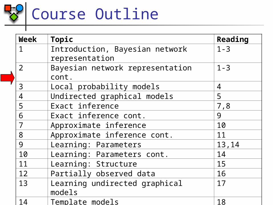
Week Topic Reading1 Introduction, Bayesian network

representation1-3

2 Bayesian network representation cont. 1-33 Local probability models 44 Undirected graphical models 55 Exact inference 7,86 Exact inference cont. 97 Approximate inference 108 Approximate inference cont. 119 Learning: Parameters 13,1410 Learning: Parameters cont. 1411 Learning: Structure 1512 Partially observed data 1613 Learning undirected graphical models 1714 Template models 1815 Dynamic Bayesian networks 18

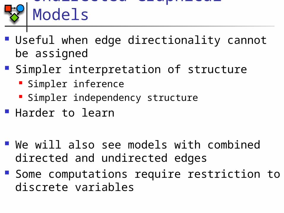
Undirected Graphical Models Useful when edge directionality cannot be

assigned Simpler interpretation of structure

Simpler inference Simpler independency structure

Harder to learn

We will also see models with combined directed and undirected edges

Some computations require restriction to discrete variables

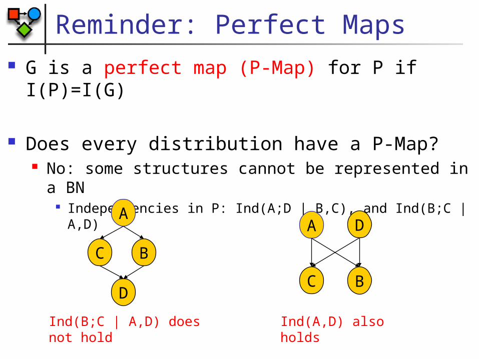
Reminder: Perfect Maps G is a perfect map (P-Map) for P if I(P)=I(G)

Does every distribution have a P-Map? No: some structures cannot be represented in a BN

Independencies in P: Ind(A;D | B,C), and Ind(B;C | A,D)

D

A

BC

Ind(B;C | A,D) does not hold

DA

BC

Ind(A,D) also holds

Representing Dependencies Ind(A;D | B,C), and Ind(B;C | A,D)

Cannot be modeled with a Bayesian network without extraneous edges

Can be modeled with an undirected (Markov) network

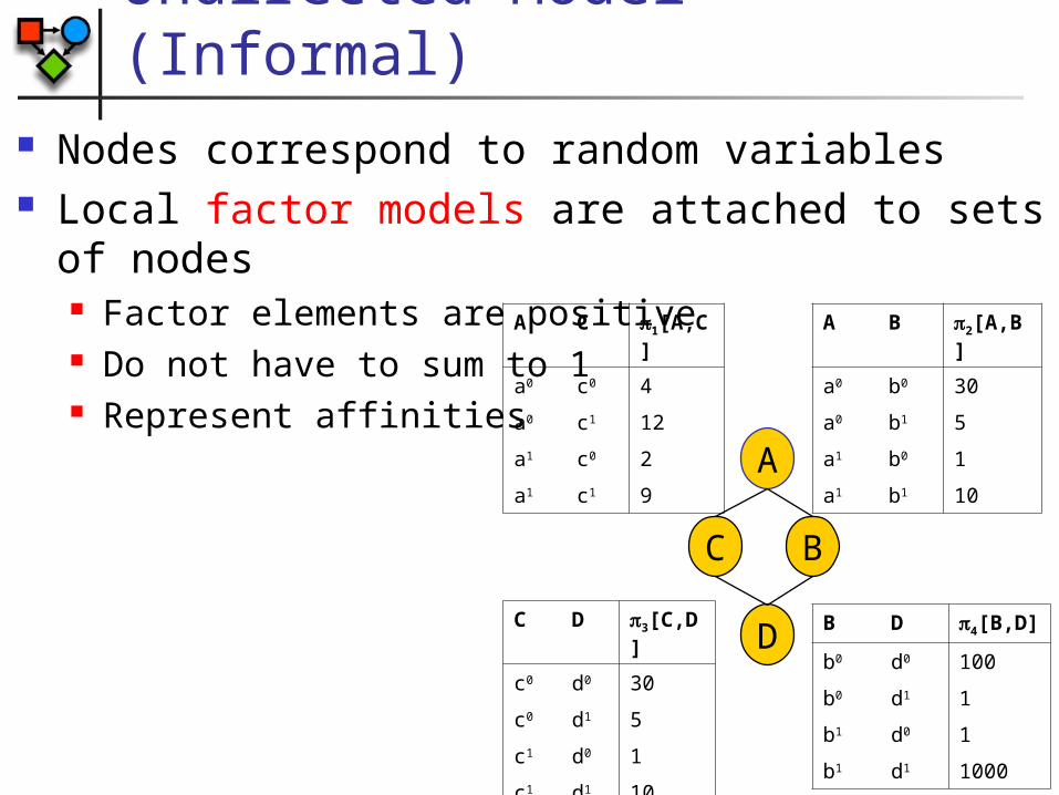
Undirected Model (Informal) Nodes correspond to random variables Local factor models are attached to sets of

nodes Factor elements are positive Do not have to sum to 1 Represent affinities

D

A

BC

A C 1[A,C]

a0 c0 4

a0 c1 12

a1 c0 2

a1 c1 9

A B 2[A,B]

a0 b0 30

a0 b1 5

a1 b0 1

a1 b1 10

C D 3[C,D]

c0 d0 30

c0 d1 5

c1 d0 1

c1 d1 10

B D 4[B,D]

b0 d0 100

b0 d1 1

b1 d0 1

b1 d1 1000

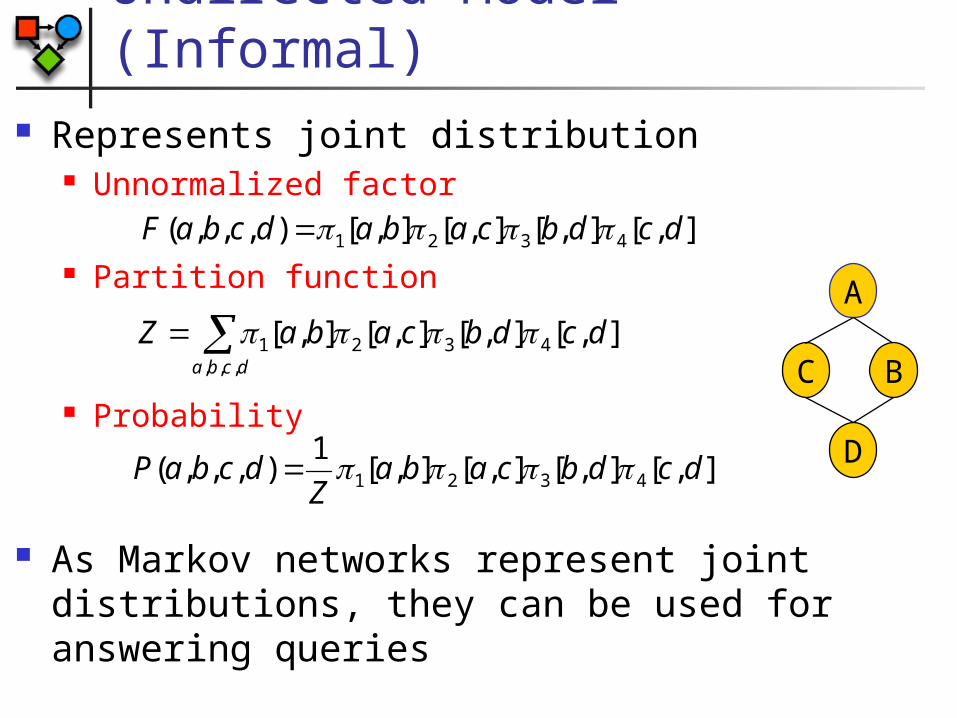
Undirected Model (Informal) Represents joint distribution

Unnormalized factor

Partition function

Probability

As Markov networks represent joint distributions, they can be used for answering queries

D

A

BC

],[],[],[],[),,,( 4321 dcdbcabadcbaF

dcba

dcdbcabaZ,,,

4321 ],[],[],[],[

],[],[],[],[1

),,,( 4321 dcdbcabaZ

dcbaP

Markov Network Structure Undirected graph H

Nodes X1,…,Xn represent random variables

H encodes independence assumptions A path X1,…,Xk is active if none of the Xi variables

along the path are observed X and Y are separated in H given Z if there is no

active path between any node xX and any node yY given Z

Denoted sepH(X;Y|Z)B

C

A DD {A,C} | B

Global Markov assumptions: I(H) = {(XY|Z) : sepH(X;Y|Z)}

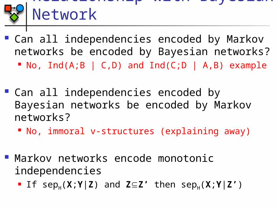
Relationship with Bayesian Network

Can all independencies encoded by Markov networks be encoded by Bayesian networks? No, Ind(A;B | C,D) and Ind(C;D | A,B) example

Can all independencies encoded by Bayesian networks be encoded by Markov networks? No, immoral v-structures (explaining away)

Markov networks encode monotonic independencies If sepH(X;Y|Z) and ZZ’ then sepH(X;Y|Z’)

Markov Network Factors A factor is a function from value assignments of

a set of random variables D to real positive numbers +

The set of variables D is the scope of the factor

Factors generalize the notion of CPDs Every CPD is a factor (with additional constraints)

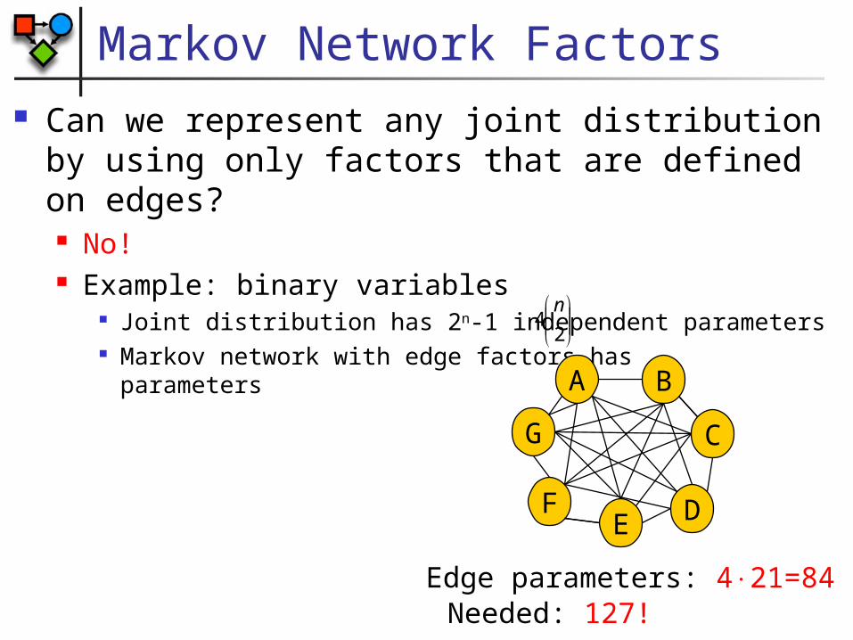
Markov Network Factors Can we represent any joint distribution by

using only factors that are defined on edges? No! Example: binary variables

Joint distribution has 2n-1 independent parameters Markov network with edge factors has parameters

2

4n

B

D

A

C

EF

G

Edge parameters: 421=84 Needed: 127!

Markov Network Factors Are there constraints imposed on the network

structure H by a factor whose scope is D? Hint 1: think of the independencies that must be

satisfied Hint 2: generalize from the basic case of |D|=2

The induced subgraph over D must be a clique (fully connected)(otherwise two unconnected variables may be independent byblocking the active path between them, contradicting the direct

dependency between them in the factor over D)

Markov Network Factors

C

A

DB

C

A

DB

Maximal cliques {A,B} {B,C} {C,D} {A,D}

Maximal cliques {A,B,C} {A,C,D}

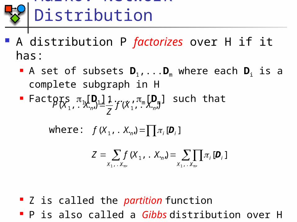
Markov Network Distribution A distribution P factorizes over H if it has:

A set of subsets D1,...Dm where each Di is a complete subgraph in H

Factors 1[D1],...,m[Dm] such that

Z is called the partition function P is also called a Gibbs distribution over H

),...,(1

),...,( 11 nn XXfZ

XXP

][),...,( 1 iinXXf D

nn XX

iiXX

nXXfZ,...,,...,

1

11

][),...,( D

where:

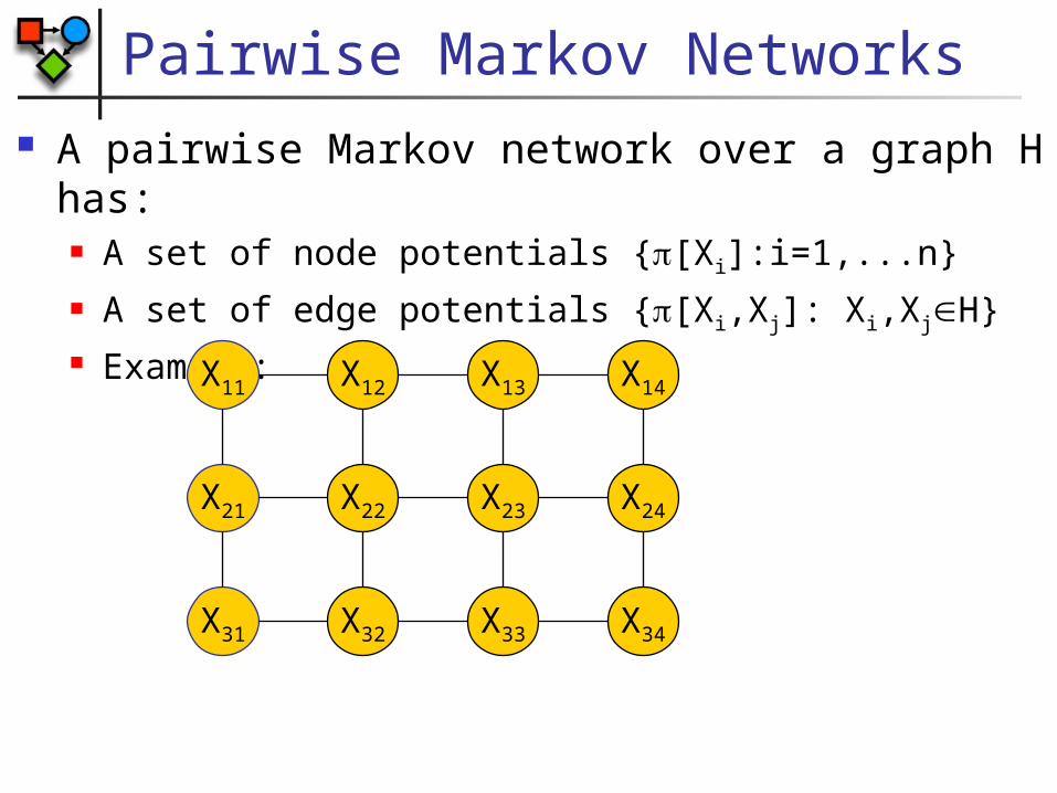
Pairwise Markov Networks A pairwise Markov network over a graph H has:

A set of node potentials {[Xi]:i=1,...n} A set of edge potentials {[Xi,Xj]: Xi,XjH} Example:

X11 X12 X13 X14

X21 X22 X23 X24

X31 X32 X33 X34

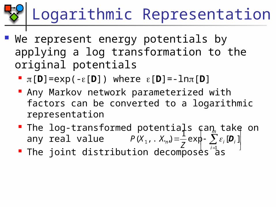
Logarithmic Representation We represent energy potentials by applying a

log transformation to the original potentials [D]=exp(-[D]) where [D]=-ln[D] Any Markov network parameterized with factors can

be converted to a logarithmic representation The log-transformed potentials can take on any real

value The joint distribution decomposes as

m

iiin Z

XXP1

1 ][exp1

),...,( D

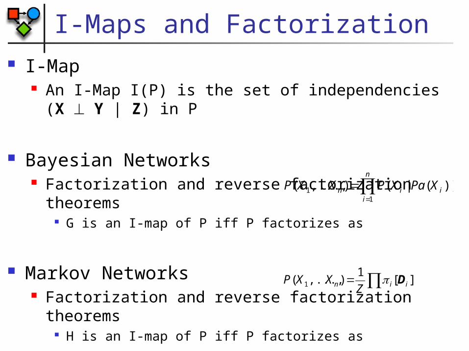
I-Maps and Factorization I-Map

An I-Map I(P) is the set of independencies (X Y | Z) in P

Bayesian Networks Factorization and reverse factorization theorems

G is an I-map of P iff P factorizes as

Markov Networks Factorization and reverse factorization theorems

H is an I-map of P iff P factorizes as

n

iiin XPaXPXXP

11 ))(|(),...,(

][1

),...,( 1 iin ZXXP D

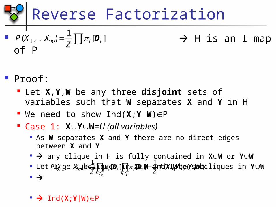
Reverse Factorization H is an I-map of P

Proof: Let X,Y,W be any three disjoint sets of variables

such that W separates X and Y in H We need to show Ind(X;Y|W)P Case 1: XYW=U (all variables)

As W separates X and Y there are no direct edges between X and Y

any clique in H is fully contained in XW or YW Let IX be subcliques in XW and IY be subcliques in YW

Ind(X;Y|W)P

][1

),...,( 1 iin ZXXP D

),(),(1

][][1

),...,( 1 WYWXDDYX

gfZZ

XXPIi

iiIi

iin

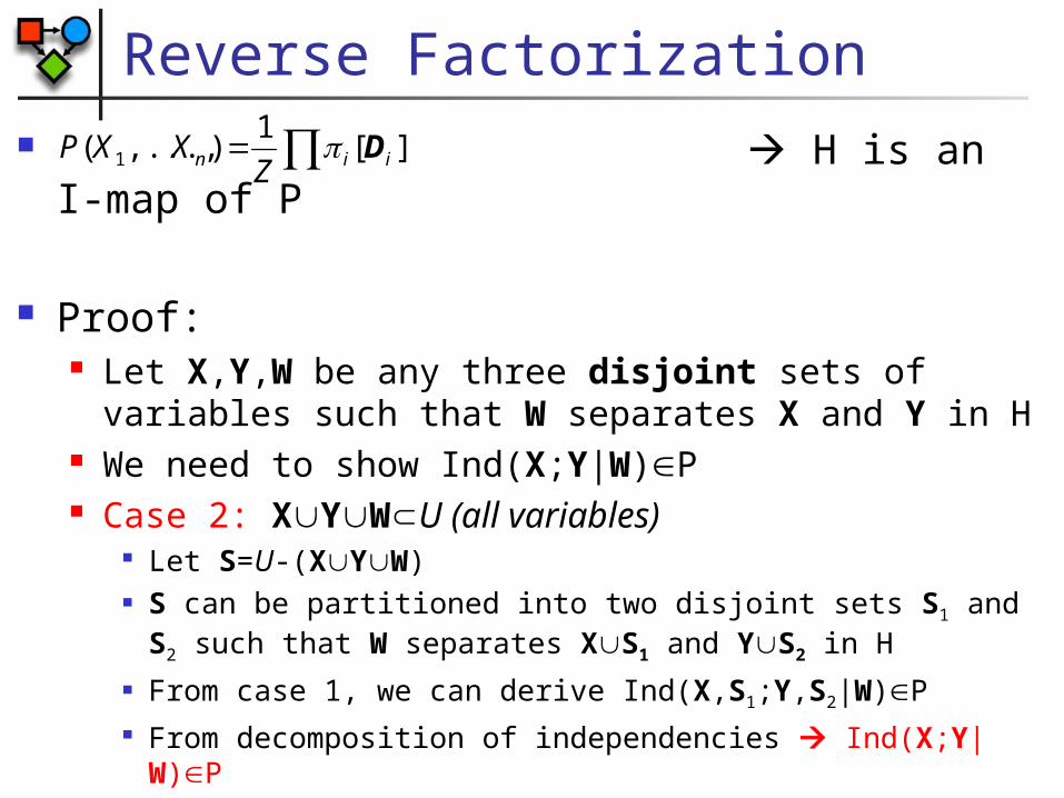
Reverse Factorization H is an I-map of P

Proof: Let X,Y,W be any three disjoint sets of variables

such that W separates X and Y in H We need to show Ind(X;Y|W)P Case 2: XYWU (all variables)

Let S=U-(XYW) S can be partitioned into two disjoint sets S1 and S2 such

that W separates XS1 and YS2 in H From case 1, we can derive Ind(X,S1;Y,S2|W)P From decomposition of independencies Ind(X;Y|W)P

][1

),...,( 1 iin ZXXP D

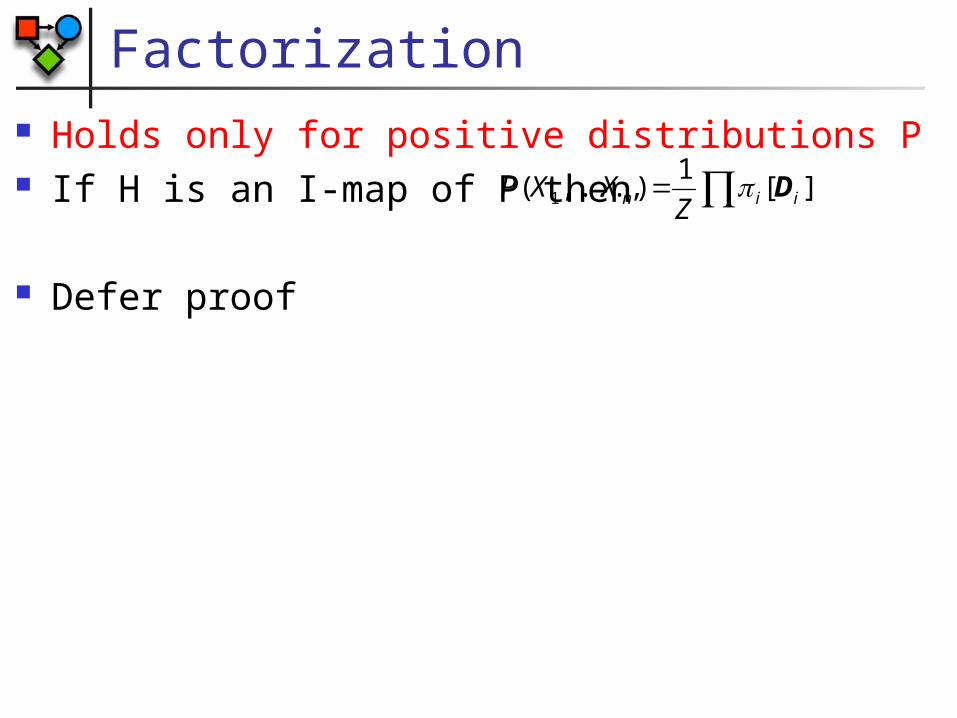
Factorization Holds only for positive distributions P If H is an I-map of P then

Defer proof

][1

),...,( 1 iin ZXXP D

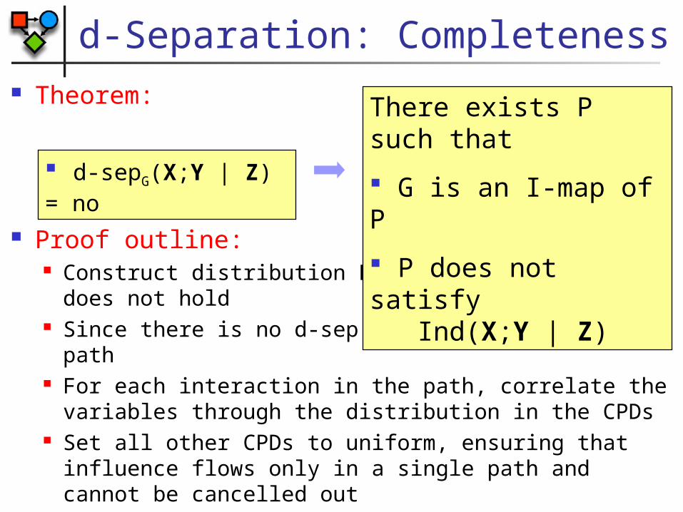
d-Separation: Completeness Theorem:

Proof outline: Construct distribution P where independence does

not hold Since there is no d-sep, there is an active path For each interaction in the path, correlate the

variables through the distribution in the CPDs Set all other CPDs to uniform, ensuring that

influence flows only in a single path and cannot be cancelled out

d-sepG(X;Y | Z) = no

There exists P such that

G is an I-map of P

P does not satisfy Ind(X;Y | Z)

Separation: Completeness Theorem:

Proof outline: Construct distribution P where independence does

not hold Since there is no sep, there is an active path For each interaction in the path, correlate the

variables through the potentials Set all other potentials to uniform, ensuring that

influence flows only in a single path and cannot be cancelled out

sepH(X;Y | Z) = no

There exists P such that

H is an I-map of P

P does not satisfy Ind(X;Y | Z)

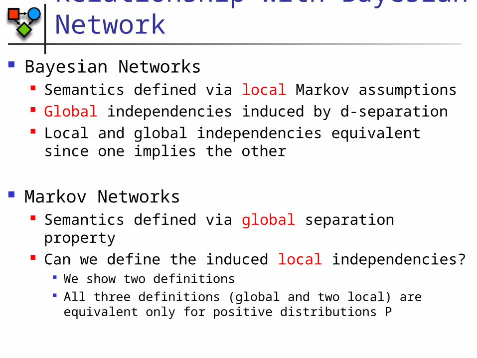
Relationship with Bayesian Network

Bayesian Networks Semantics defined via local Markov assumptions Global independencies induced by d-separation Local and global independencies equivalent since

one implies the other

Markov Networks Semantics defined via global separation property Can we define the induced local independencies?

We show two definitions All three definitions (global and two local) are equivalent

only for positive distributions P

Pairwise Markov Independencies

Every pair of disconnected nodes are separated given all other nodes in the network

Formally: IP(H) = {(XY|U-{X,Y}) : X—YH}

D

A

BC

Example:

Ind(A;D | B,C,E)

Ind(B;C | A,D,E)

Ind(D;E | A,B,C)

E

Markov Blanket Independencies

Every node is independent of all other nodes given its immediate neighboring nodes in the network

Formally: IL(H) = {(XU-{X}-NH(X)|NH(X)) : XH}

D

A

BC

Example:

Ind(A;D | B,C,E)

Ind(B;C | A,D,E)

Ind(C;B | A,D,E)

Ind(D;E,A | B,C)

Ind(E;D | A,B,C)

E

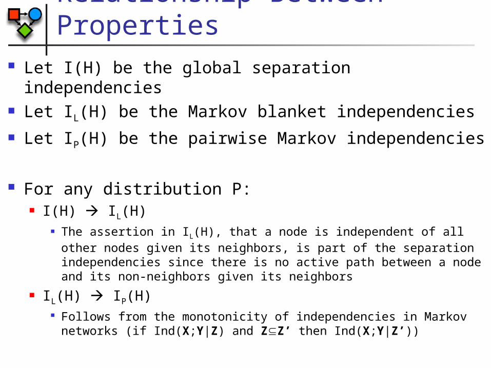
Relationship Between Properties

Let I(H) be the global separation independencies

Let IL(H) be the Markov blanket independencies Let IP(H) be the pairwise Markov independencies

For any distribution P: I(H) IL(H)

The assertion in IL(H), that a node is independent of all other nodes given its neighbors, is part of the separation independencies since there is no active path between a node and its non-neighbors given its neighbors

IL(H) IP(H) Follows from the monotonicity of independencies in Markov

networks (if Ind(X;Y|Z) and ZZ’ then Ind(X;Y|Z’))

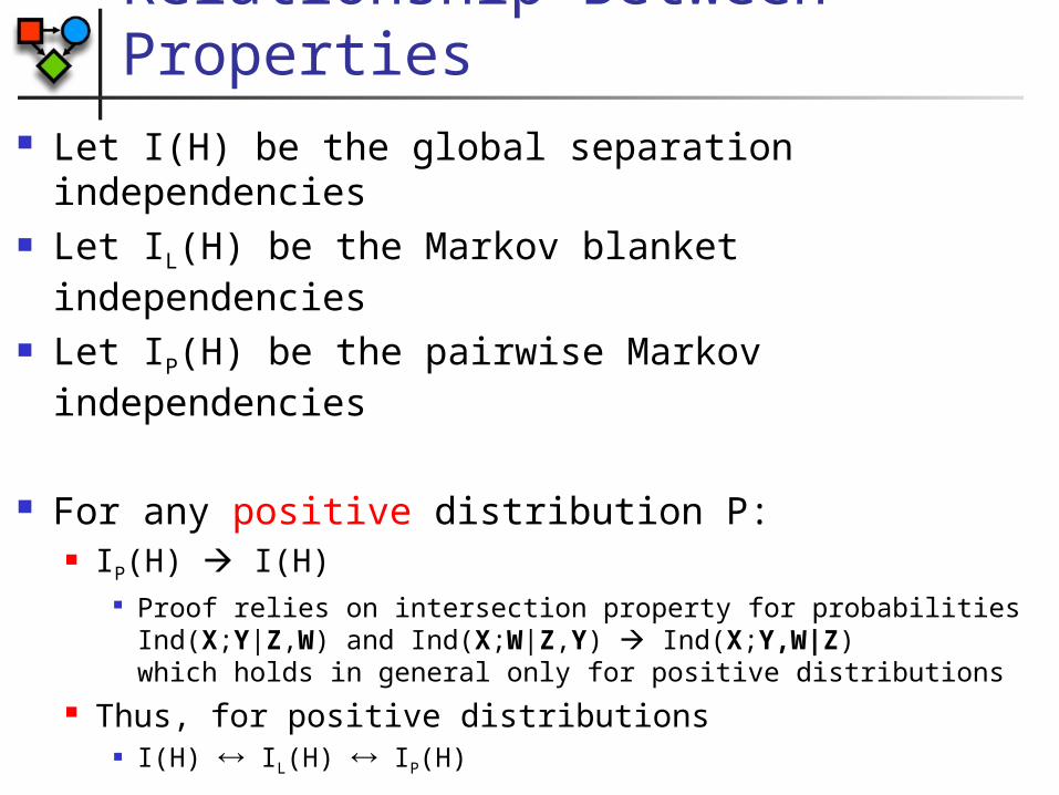
Relationship Between Properties

Let I(H) be the global separation independencies

Let IL(H) be the Markov blanket independencies Let IP(H) be the pairwise Markov

independencies

For any positive distribution P: IP(H) I(H)

Proof relies on intersection property for probabilitiesInd(X;Y|Z,W) and Ind(X;W|Z,Y) Ind(X;Y,W|Z)which holds in general only for positive distributions

Thus, for positive distributions I(H) IL(H) IP(H)

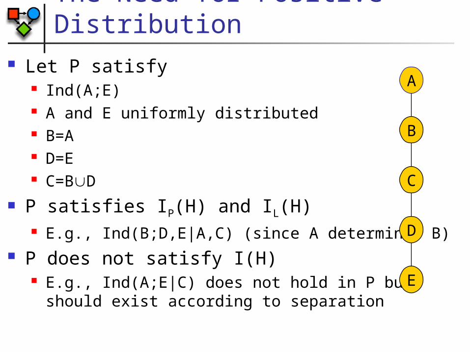
The Need for Positive Distribution

Let P satisfy Ind(A;E) A and E uniformly distributed B=A D=E C=BD

P satisfies IP(H) and IL(H) E.g., Ind(B;D,E|A,C) (since A determines B)

P does not satisfy I(H) E.g., Ind(A;E|C) does not hold in P but

should exist according to separation

D

A

B

C

E

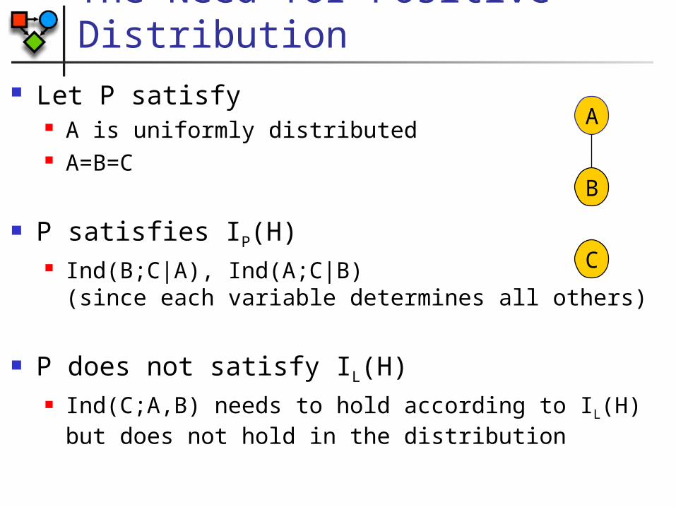
The Need for Positive Distribution

Let P satisfy A is uniformly distributed A=B=C

P satisfies IP(H) Ind(B;C|A), Ind(A;C|B)

(since each variable determines all others)

P does not satisfy IL(H) Ind(C;A,B) needs to hold according to IL(H) but does

not hold in the distribution

A

B

C

Constructing Markov Network for P

Goal: Given a distribution, we want to construct a Markov network which is an I-map of P

Complete graphs will satisfy but are not interesting

Minimal I-maps: A graph G is a minimal I-Map for P if: G is an I-map for P Removing any edge from G renders it not an I-map

Goal: construct a graph which is a minimal I-map of P

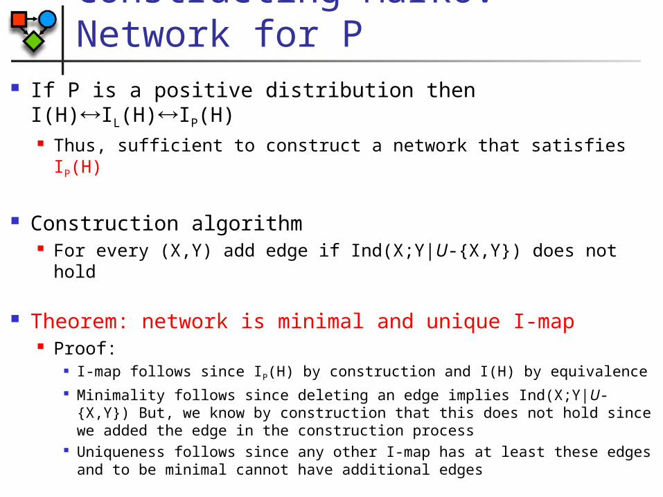
Constructing Markov Network for P

If P is a positive distribution then I(H)IL(H)IP(H) Thus, sufficient to construct a network that satisfies IP(H)

Construction algorithm For every (X,Y) add edge if Ind(X;Y|U-{X,Y}) does not hold

Theorem: network is minimal and unique I-map Proof:

I-map follows since IP(H) by construction and I(H) by equivalence Minimality follows since deleting an edge implies Ind(X;Y|U-{X,Y})

But, we know by construction that this does not hold since we added the edge in the construction process

Uniqueness follows since any other I-map has at least these edges and to be minimal cannot have additional edges

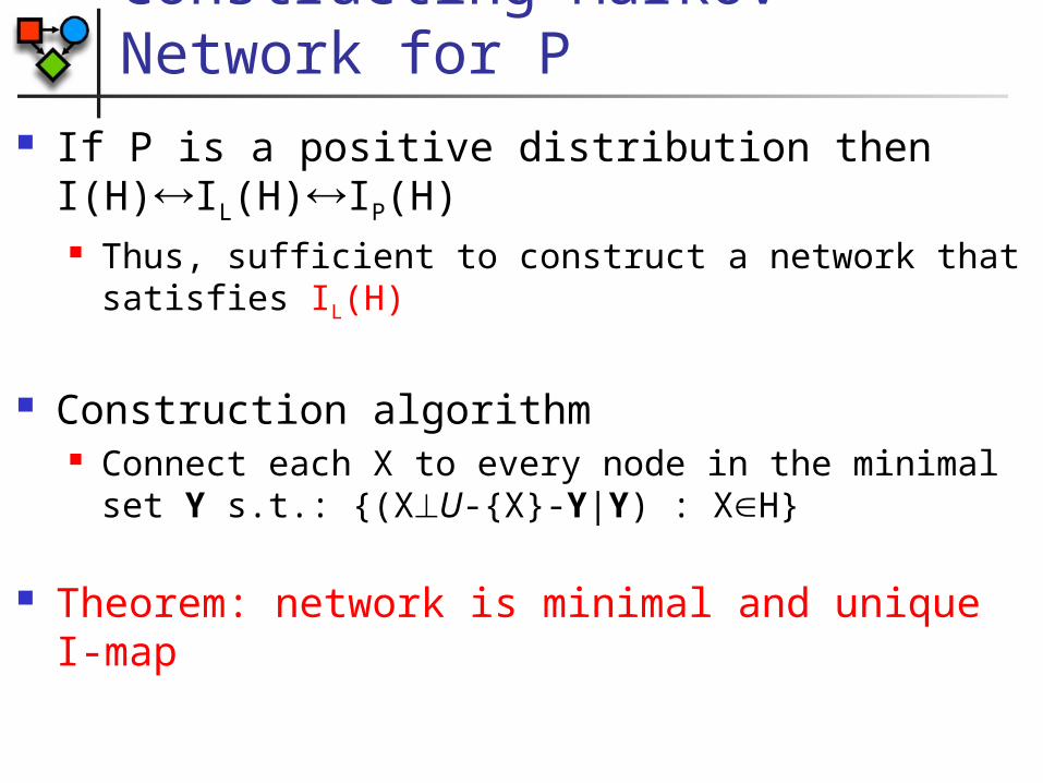
Constructing Markov Network for P

If P is a positive distribution then I(H)IL(H)IP(H) Thus, sufficient to construct a network that satisfies

IL(H)

Construction algorithm Connect each X to every node in the minimal set Y

s.t.: {(XU-{X}-Y|Y) : XH}

Theorem: network is minimal and unique I-map

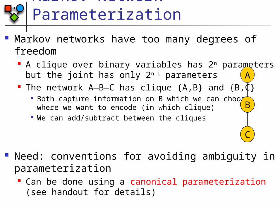
Markov Network Parameterization

Markov networks have too many degrees of freedom A clique over binary variables has 2n parameters but

the joint has only 2n-1 parameters The network A—B—C has clique {A,B} and {B,C}

Both capture information on B which we can choosewhere we want to encode (in which clique)

We can add/subtract between the cliques

Need: conventions for avoiding ambiguity in parameterization Can be done using a canonical parameterization

(see handout for details)

A

B

C

Factor Graphs From the Markov network structure we do not

know whether parameterization involves maximal cliques Example: fully connected graph may be pairwise

potentials or one large (exponential) potential over all nodes

Solution: Factor Graphs Undirected graph Two types of nodes

Variable nodes Factor nodes

Parameterization Each factor node is associated with exactly one factor Scope of factor are all neighbor variables of the factor node

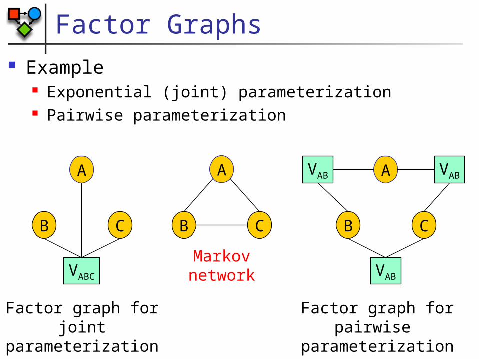
Factor Graphs Example

Exponential (joint) parameterization Pairwise parameterization

A

B C

A

B C

VABC

Factor graph forjoint parameterization

A

B C

VAB VAB

VAB

Factor graph forpairwise parameterization

Markov network

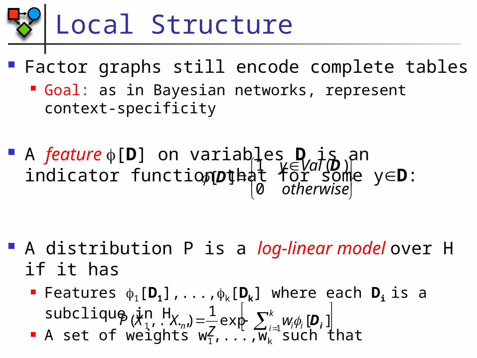
Local Structure Factor graphs still encode complete tables

Goal: as in Bayesian networks, represent context-specificity

A feature [D] on variables D is an indicator function that for some yD:

A distribution P is a log-linear model over H if it has Features 1[D1],...,k[Dk] where each Di is a subclique

in H A set of weights w1,...,wk such that

otherwise

Valy

0

)(1][

DD

k

i iin wZ

XXP11 ][exp

1),...,( iD

Feature Representation Several features can be defined on one

subclique any factor can be represented by features, where

in the most general case we define a feature and weight for each entry in the factor

Log-linear model is more compact for many distributions especially with large domain variables

Representation is intuitive and modular Features can be modularly added between any

interacting sets of variables

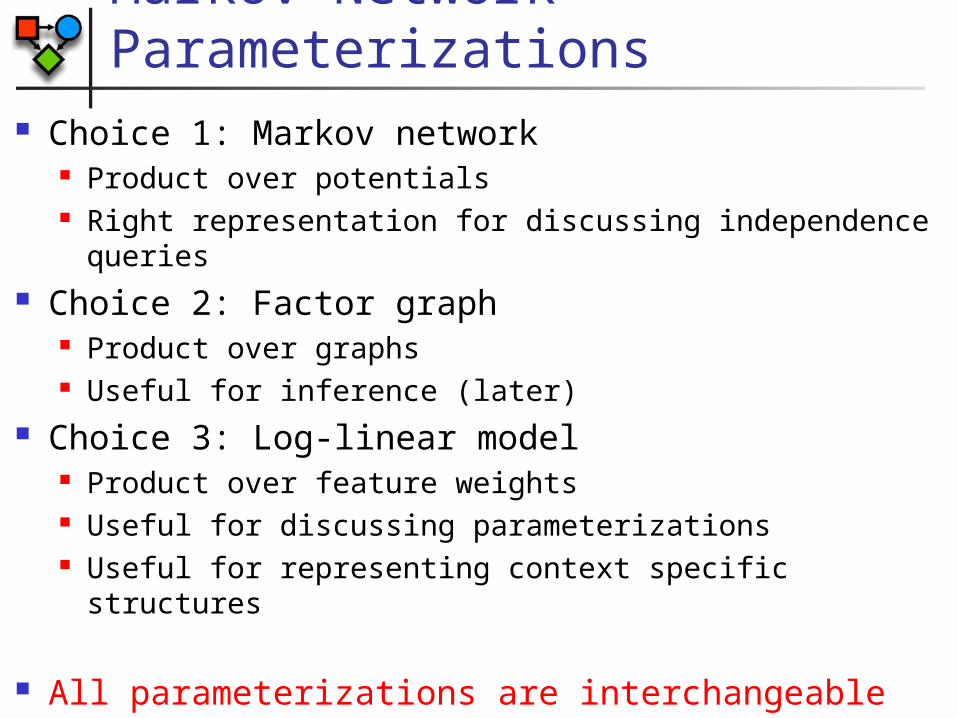
Markov Network Parameterizations

Choice 1: Markov network Product over potentials Right representation for discussing independence

queries Choice 2: Factor graph

Product over graphs Useful for inference (later)

Choice 3: Log-linear model Product over feature weights Useful for discussing parameterizations Useful for representing context specific structures

All parameterizations are interchangeable

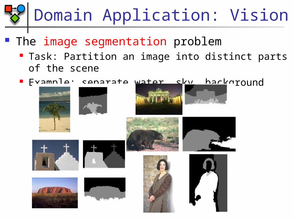
Domain Application: Vision The image segmentation problem

Task: Partition an image into distinct parts of the scene

Example: separate water, sky, background

Markov Network for Segmentation

Grid structured Markov network Random variable Xi corresponds to pixel i

Domain is {1,...K} Value represents region assignment to pixel i

Neighboring pixels are connected in the network Appearance distribution

wik – extent to which pixel i “fits” region k (e.g.,

difference from typical pixel for region k) Introduce node potential exp(-wi

k1{Xi=k})

Edge potentials Encodes contiguity preference by edge potential

exp(1{Xi=Xj}) for >0

Markov Network for Segmentation

Solution: inference Find most likely assignment to Xi variables

X11 X12 X13 X14

X21 X22 X23 X24

X31 X32 X33 X34

Appearance distribution

Contiguity preference

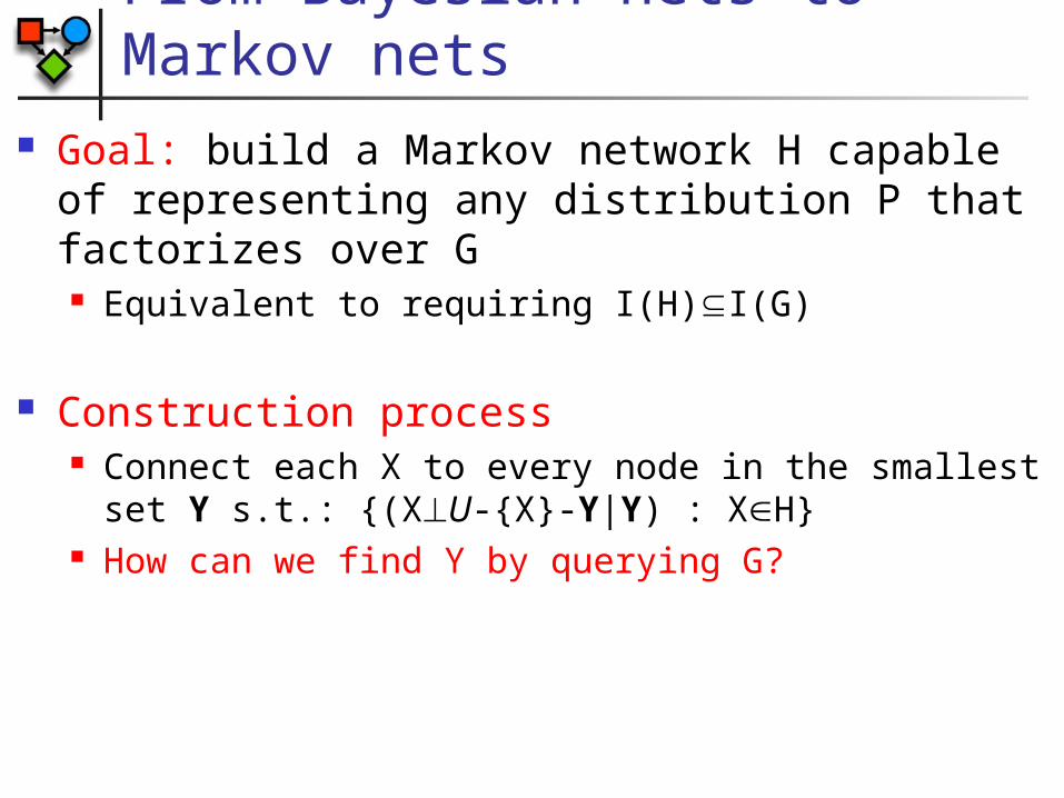
From Bayesian nets to Markov nets

Goal: build a Markov network H capable of representing any distribution P that factorizes over G Equivalent to requiring I(H)I(G)

Construction process Connect each X to every node in the smallest set Y

s.t.: {(XU-{X}-Y|Y) : XH} How can we find Y by querying G?

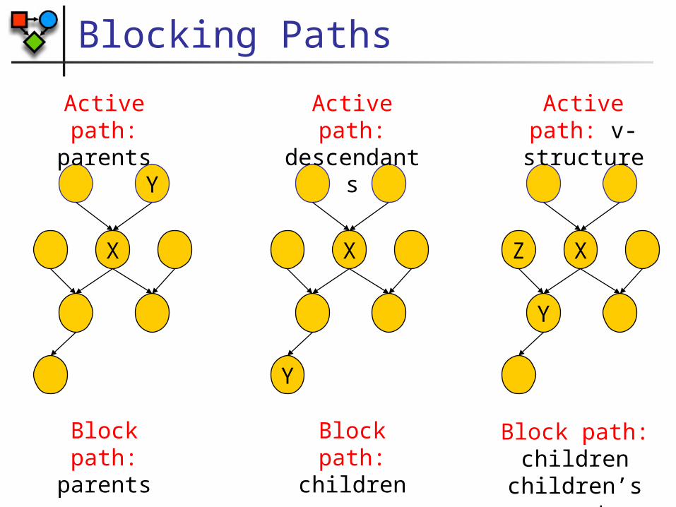
Blocking Paths

X

Y

X

Y

Y

XZ

Active path: parents

Active path: descendants

Active path: v-structure

Block path: parents

Block path: children

Block path:children

children’s parents

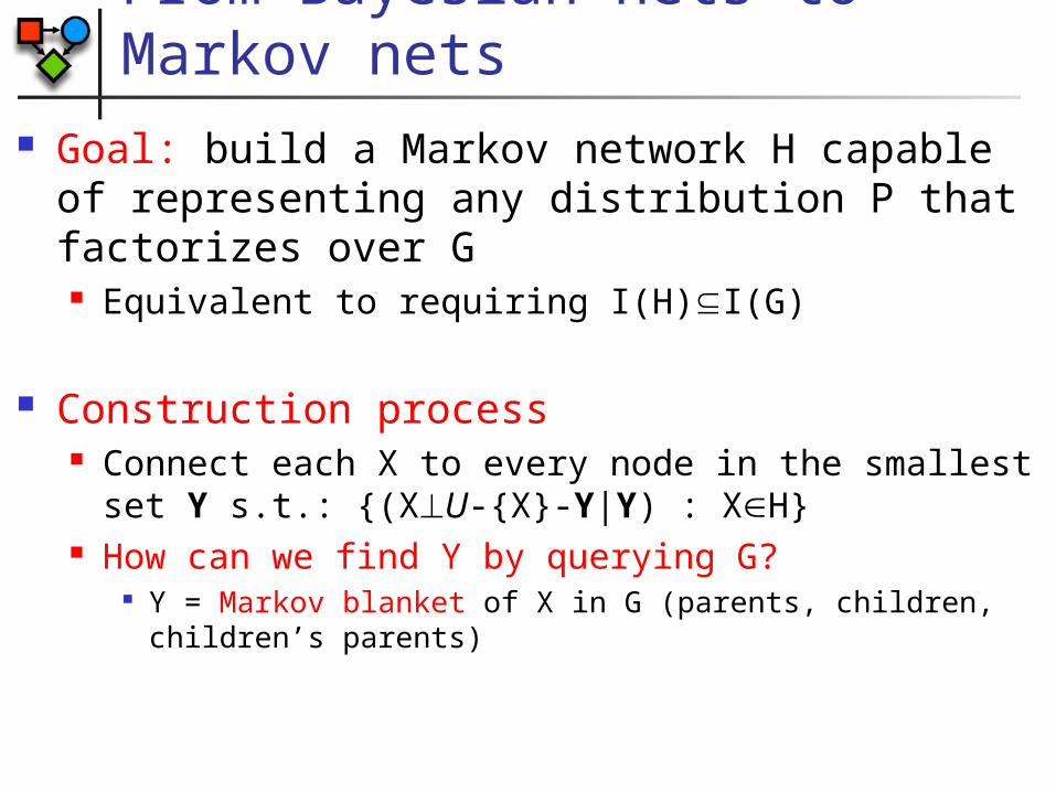
From Bayesian nets to Markov nets

Goal: build a Markov network H capable of representing any distribution P that factorizes over G Equivalent to requiring I(H)I(G)

Construction process Connect each X to every node in the smallest set Y

s.t.: {(XU-{X}-Y|Y) : XH} How can we find Y by querying G?

Y = Markov blanket of X in G (parents, children, children’s parents)

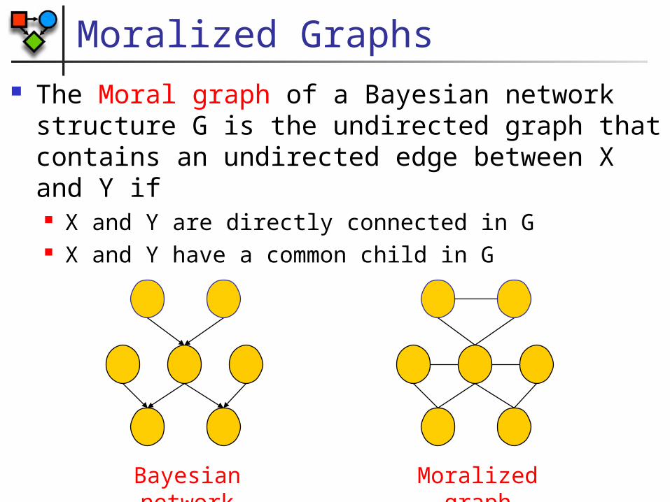
Moralized Graphs The Moral graph of a Bayesian network

structure G is the undirected graph that contains an undirected edge between X and Y if X and Y are directly connected in G X and Y have a common child in G

Bayesian network

Moralized graph

Parameterizing Moralized Graphs

Moralized graph contains a full clique for every Xi and its parents Pa(Xi) We can associate CPDs with a clique

Do we lose independence assumptions implied by the graph structure? Yes, immoral v-structures

A

C

B A

C

B

Ind(A;B)

From Markov nets to Bayesian nets

Transformation is more difficult and the resulting network can be much larger than the Markov network

Construction algorithm Use Markov network as template for independencies Fix ordering of nodes Add each node along with its minimal parent set

according to the independencies defined in the distribution

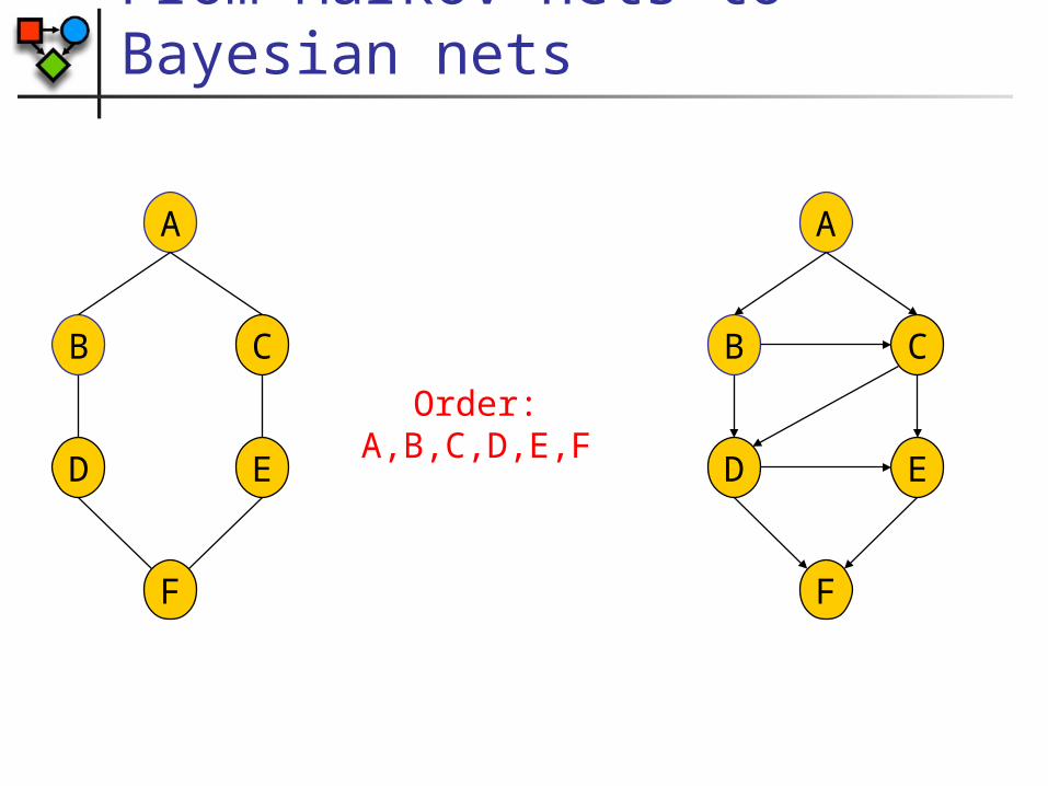
From Markov nets to Bayesian nets

A

CB

Order: A,B,C,D,E,F

ED

F

A

CB

ED

F

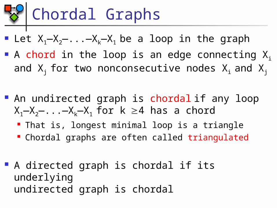
Chordal Graphs Let X1—X2—...—Xk—X1 be a loop in the graph A chord in the loop is an edge connecting Xi

and Xj for two nonconsecutive nodes Xi and Xj

An undirected graph is chordal if any loopX1—X2—...—Xk—X1 for k4 has a chord That is, longest minimal loop is a triangle Chordal graphs are often called triangulated

A directed graph is chordal if its underlyingundirected graph is chordal

From Markov Nets to Bayesian Nets

Theorem: Let H be a Markov network structure and G be any minimal I-map for H. Then G is chordal

The process of turning a Markov network into a Bayesian network is called triangulation The process loses independencies

A

CB

ED

F

A

CB

ED

FInd(B;C|A,F)

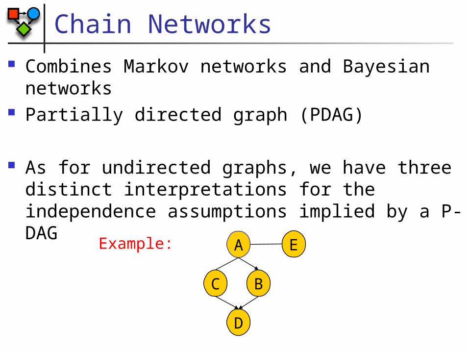
Chain Networks Combines Markov networks and Bayesian

networks Partially directed graph (PDAG)

As for undirected graphs, we have three distinct interpretations for the independence assumptions implied by a P-DAG

D

A

BC

EExample:

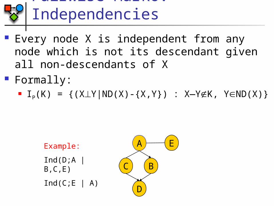
Pairwise Markov Independencies

Every node X is independent from any node which is not its descendant given all non-descendants of X

Formally: IP(K) = {(XY|ND(X)-{X,Y}) : X—YK, YND(X)}

Example:

Ind(D;A | B,C,E)

Ind(C;E | A)

D

A

BC

E

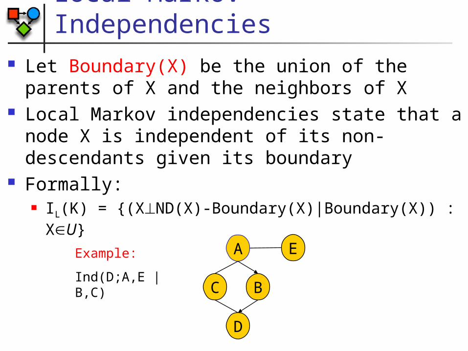
Local Markov Independencies Let Boundary(X) be the union of the parents of

X and the neighbors of X Local Markov independencies state that a node

X is independent of its non-descendants given its boundary

Formally: IL(K) = {(XND(X)-Boundary(X)|Boundary(X)) : XU}

Example:

Ind(D;A,E | B,C)

D

A

BC

E

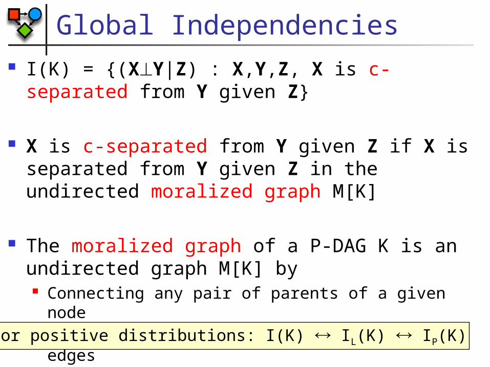
Global Independencies I(K) = {(XY|Z) : X,Y,Z, X is c-separated from

Y given Z}

X is c-separated from Y given Z if X is separated from Y given Z in the undirected moralized graph M[K]

The moralized graph of a P-DAG K is an undirected graph M[K] by Connecting any pair of parents of a given node Converting all directed edges to undirected edges

For positive distributions: I(K) IL(K) IP(K)

Application: Molecular Pathways

Pathway genes are regulated together Pathway genes physically interact

Goal Automatic discovery of molecular

pathways: sets of genes that Are regulated together Physically interact

Pathway IIPathway III

Pathway I

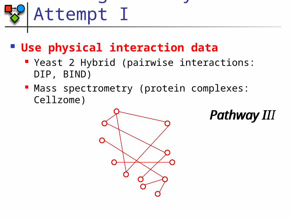
Finding Pathways: Attempt I

Use physical interaction data Yeast 2 Hybrid (pairwise interactions: DIP, BIND) Mass spectrometry (protein complexes: Cellzome)

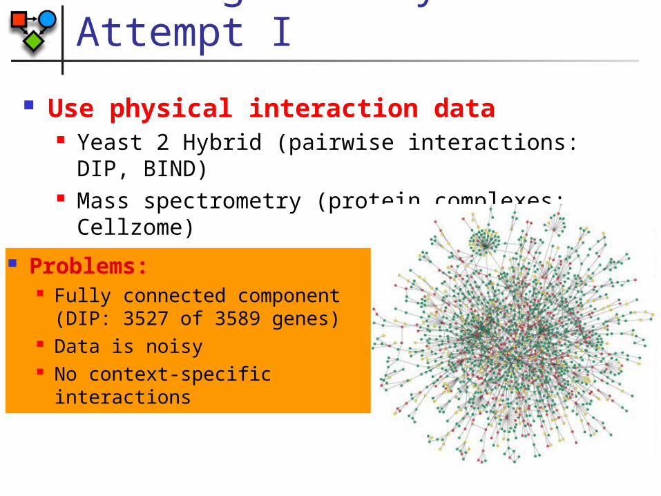
Finding Pathways: Attempt I

Use physical interaction data Yeast 2 Hybrid (pairwise interactions: DIP, BIND) Mass spectrometry (protein complexes: Cellzome)

Problems: Fully connected component

(DIP: 3527 of 3589 genes) Data is noisy No context-specific

interactions

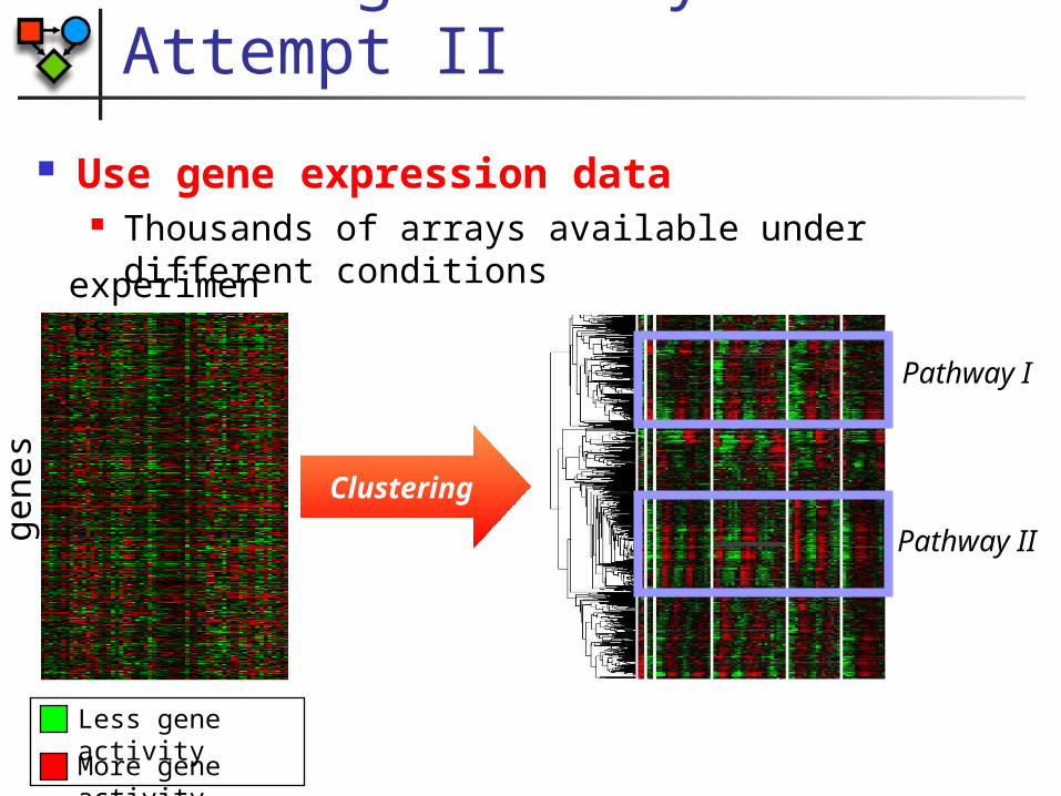
Finding Pathways: Attempt II

Use gene expression data Thousands of arrays available under different

conditions

Clustering

Pathway I

Pathway II

experiments

gene

s

Less gene activity

More gene activity

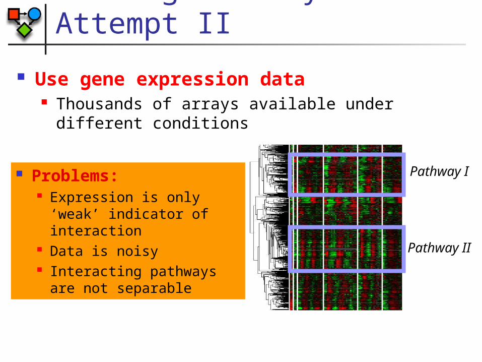
Finding Pathways: Attempt II

Use gene expression data Thousands of arrays available under different

conditions

Pathway I

Pathway II

Problems: Expression is only ‘weak’

indicator of interaction Data is noisy Interacting pathways are

not separable

Use both types of data to find pathways Find “active” interactions using gene expression Find pathway-related co-expression using

interactions

Pathway I

Pathway II

Pathway III

Pathway IV

Finding Pathways: Our Approach

Probabilistic Model

Genes are partitioned into “pathways”: Every gene is assigned to one of ‘k’ pathways Random variable for each gene with domain {1,

…,k} Expression component:

Model likelihood is higher when genes in the same pathway have similar expression profiles

Interaction component: Model likelihood is higher when genes in the same

pathway interact

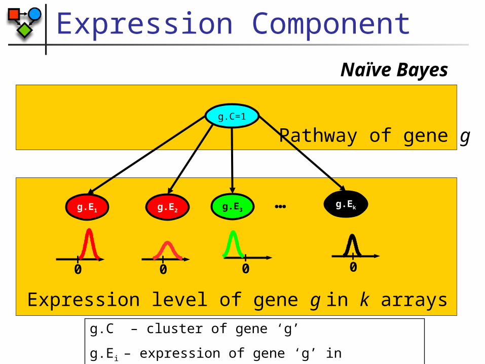
Expression Component

g.C=1

Naïve Bayes

Pathway of gene g

0 0

g.E1 g.E2 g.Ekg.E3 …

Expression level of gene g in k arrays

0 0

g.C – cluster of gene ‘g’

g.Ei – expression of gene ‘g’ in experiment i

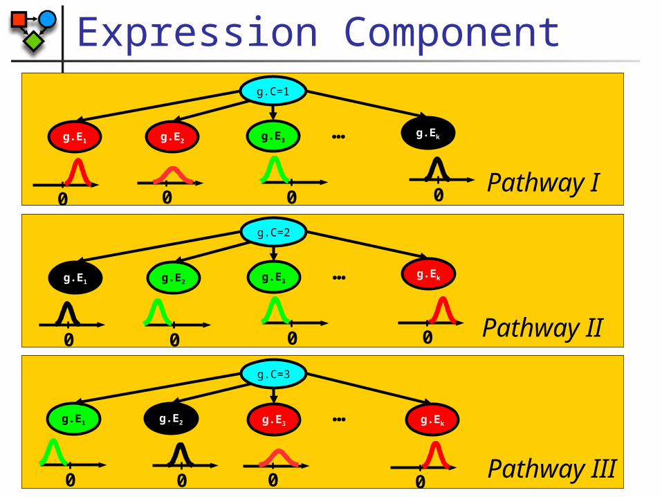
Expression Component

0 0

g.C=1

g.E1 g.E2g.Ekg.E3 …

0 0

0

g.C=2

g.E1 g.E2g.Ekg.E3 …

0

0 0

g.C=3

g.Ekg.E3g.E2g.E1 …

00

00

Pathway I

Pathway II

Pathway III

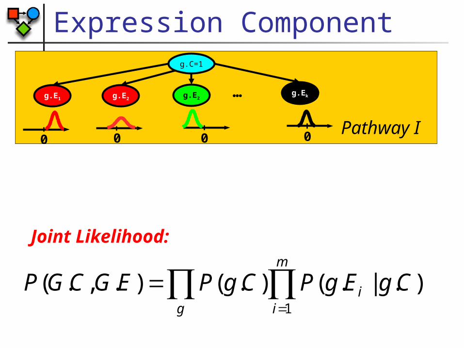
Expression Component

0 0

g.C=1

g.E1 g.E2g.Ekg.E2 …

0 0Pathway I

).|.().().,.(1

CgEgPCgPEGCGPg

m

ii

Joint Likelihood:

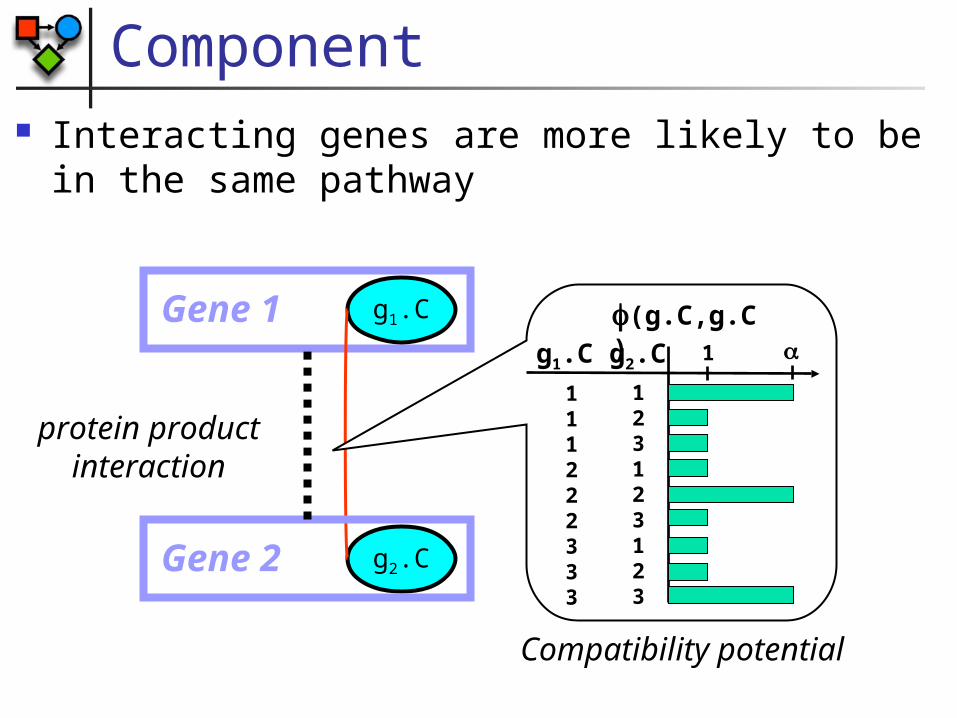
Protein Interaction Component

Gene 1

g1.C

g2.CGene 2

protein productinteraction

Interacting genes are more likely to be in the same pathway

Compatibility potential

(g.C,g.C)g1.C g2.C

123123123

111222333

1

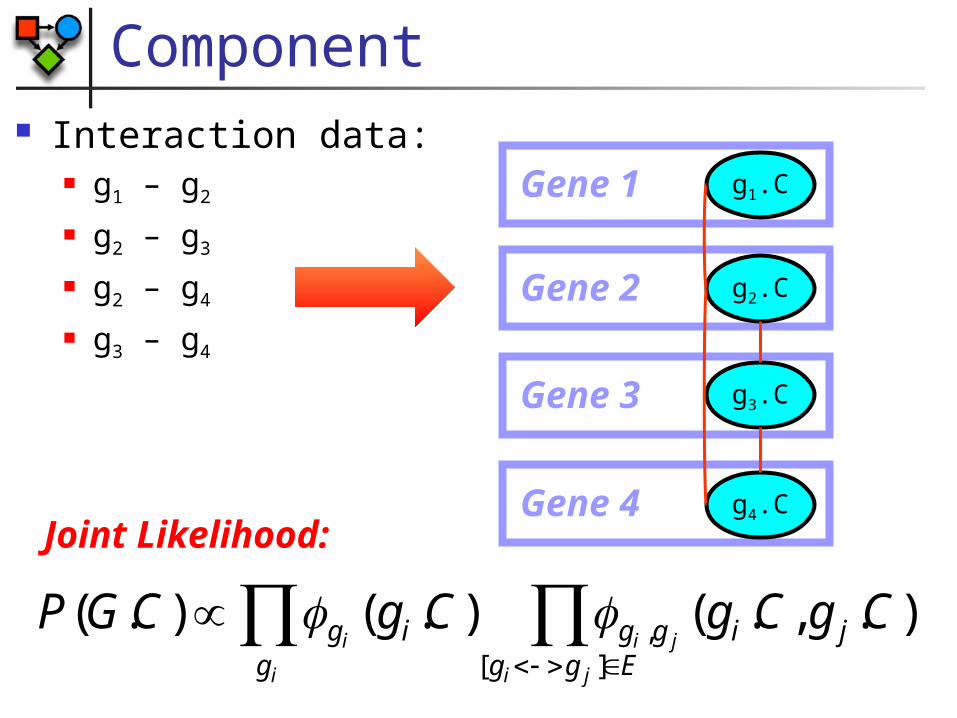
Protein Interaction Component

Interaction data: g1 – g2

g2 – g3

g2 – g4

g3 – g4

i ji

jiig Egg

jiggig CgCgCgCGP][

, ).,.().().(

Joint Likelihood:

Gene 1

g1.C

g2.C

g3.C

g4.C

Gene 2

Gene 3

Gene 4

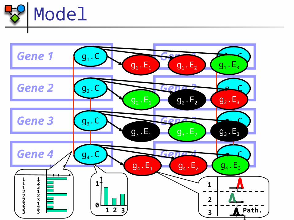
Joint Probabilistic Model

Gene 1

g1.C

g2.C

g3.C

g4.C

Gene 2

Gene 3

Gene 4

Gene 1

g1.C

g2.C

g3.C

g4.C

Gene 2

Gene 3

Gene 4

g1.E1 g1.E2 g1.E3

g2.E1 g2.E2 g2.E3

g3.E1 g3.E2 g3.E3

g4.E1 g4.E2 g4.E31

123123123

111222333 1 2 3

0

1 1

2

3

0

0

Path. I

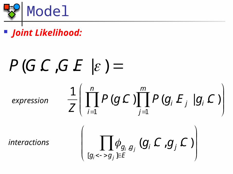
Joint Probabilistic Model Joint Likelihood:

)|.,.( EGCGP

n

i

m

jiji CgEgPCgP

Z 1 1

).|.().(1

Eggjigg

ji

jiCgCg

][, ).,.(

expression

interactions

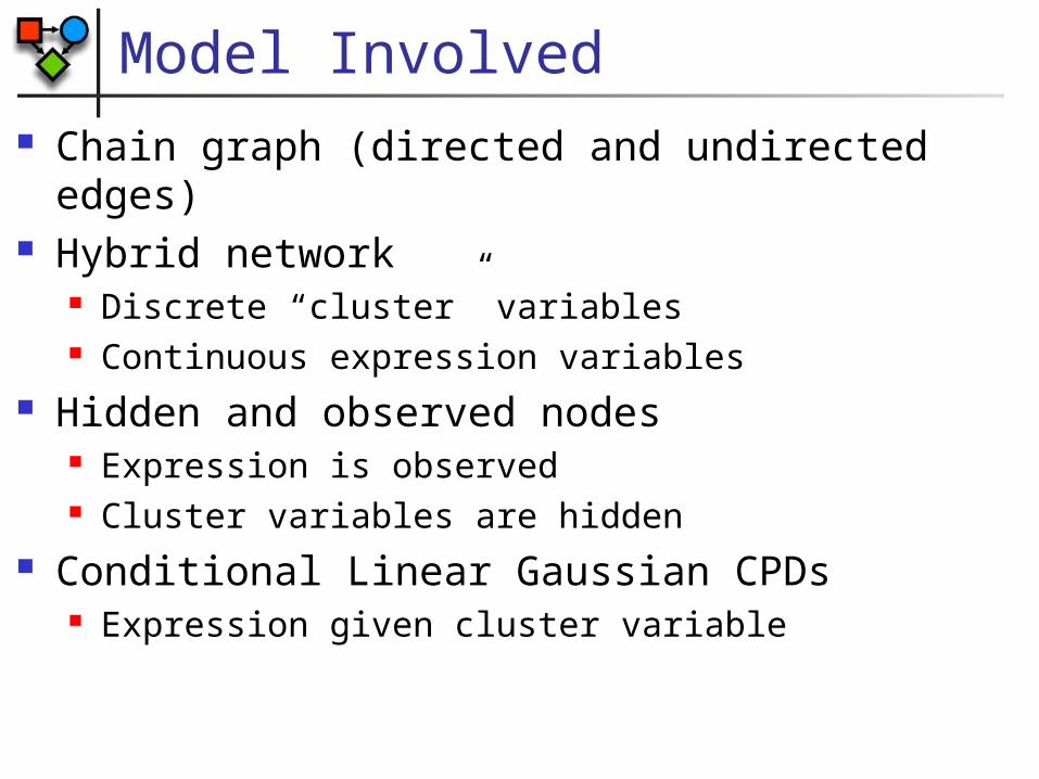
Model Involved Chain graph (directed and undirected edges) Hybrid network

Discrete “cluster” variables Continuous expression variables

Hidden and observed nodes Expression is observed Cluster variables are hidden

Conditional Linear Gaussian CPDs Expression given cluster variable

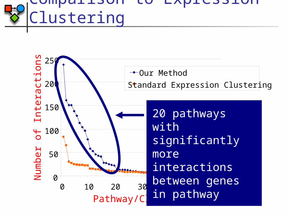
Comparison to Expression Clustering

0

50

100

150

200

250

0 10 20 30 40 50 60

Pathway/Cluster

Num

ber

of I

nter

actio

ns Our Method

Standard Expression Clustering

20 pathways with significantly more interactions between genes in pathway

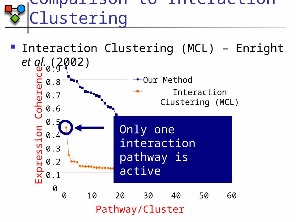
Comparison to Interaction Clustering

Pathway/Cluster

Exp

ress

ion

Coh

eren

ce

0

0.1

0.2

0.3

0.4

0.5

0.6

0.7

0.8

0.9

0 10 20 30 40 50 60

Our Method

Interaction Clustering (MCL)

Only one interaction pathway is active

Interaction Clustering (MCL) – Enright et al. (2002)

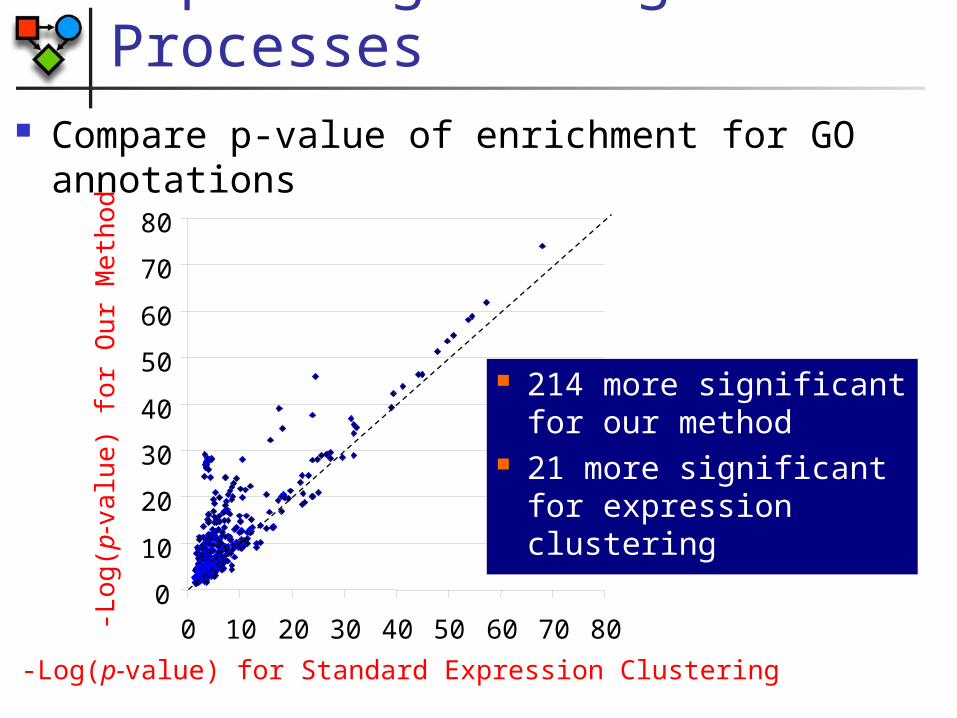
Capturing Biological Processes

Compare p-value of enrichment for GO annotations

0

10

20

30

40

50

60

70

80

0 10 20 30 40 50 60 70 80

-Log(p-value) for Standard Expression Clustering

-Log

(p-v

alu

e) fo

r O

ur M

eth

od

214 more significant for our method

21 more significant for expression clustering

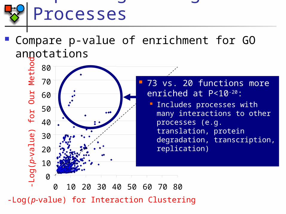
Capturing Biological Processes

Compare p-value of enrichment for GO annotations

0

10

20

30

40

50

60

70

80

0 10 20 30 40 50 60 70 80

-Log(p-value) for Interaction Clustering

-Log

(p-v

alu

e) fo

r O

ur M

eth

od

73 vs. 20 functions more enriched at P<10-20: Includes processes with

many interactions to other processes (e.g. translation, protein degradation, transcription, replication)

Summary Markov Networks – undirected graphical models

Like Bayesian networks, define independence assumptions

Three definitions exist, all equivalent in positive distributions

Factorization is defined as product of factors over complete subsets of the graph

Relationship to Bayesian networks Represent different families of independencies Independencies that can be represented in both – chordal

graphs Moralized graphs

Minimal network that represents Bayesnets dependencies d-separation in Bayesnets is equivalent to separation in

moral graphs