the open-source air pollution project - openairairtrack.lancs.ac.uk/carslaw.pdf · the open-source...

Introduction Examples of openair functions Developments and concluding remarks

The open-source air pollution projectopenair

David Carslaw and Karl Ropkins

Towards Smarter Air Quality Analysis1 October 2009

David Carslaw and Karl Ropkins — The open-source air pollution project 1/25


Outline

1 Introduction

2 Examples of openair functions

3 Developments and concluding remarks



Outline

1 Introduction





Opportunities and barriersAnalysis of measurement and model output data

Opportunities

The analysis of air quality data can provide importantinsights into air pollution

Huge amount of data available — but under used

Insightful analysis provides evidence and can revealunexpected behaviours

Barriers

No consistent set of tools available to carry out analysis

Tools can be spread across many different softwareapplications

Many useful approaches are simply unavailable

Lack of time, money or ideas about what can be done



The challenge. . .

date

NO

X (

ppb)

0

200

400

600

Jan−02 Feb−02 Mar−02 Apr−02 May−02 Jun−02 Jul−02 Aug−02 Sep−02 Oct−02 Nov−02 Dec−02

NOX

How to extract meaning and useful information from this?



The openair projectSummary of project

Key points

3-year NERC project to October 2011

With additional funding from Defra, AEA and severallocal authorities

Develop and make available open-source data analysistools to air quality community

Backed up with case studies to show usage and helpwith appropriate interpretation

Use R statistical software as the platform

Highly capable software for “programming with data”Develop a “package” of tools and progressively includeadvanced methods not widely availableOpen-source, free and very well supported



Why open-source?The benefits of an open-source approach

Availability of the source code, the rightto modify it and use it for any purpose

Allow scrutiny of methods used

Maximise user input through the abilityto contribute and improve the code

Builds trust — no ‘black boxes’ andanalysis can easily be made reproducible

Ideal for fully-engaged knowledgeexchange (key to NERC funding)

Through R there are excellentopportunities for internationalcollaboration and dissemination

OPEN sourc

e



openair websiteCentral resource for the project

Available atwww.openair-project.org

openair package –development version

All documentation, data setsetc.

News group and newslettersto keep up to date


http://www.openair-project.org


Data analysisHow best to analyse data?

John Tukey sums it up:

“The combination of some data and an achingdesire for an answer does not ensure that areasonable answer can be extracted from a givenbody of data.”

Data analysis is most useful when built around specificquestions (need an aching desire), however. . .

Exploratory data analysis can be very insightful and isunder-used — but time consuming

Case studies can provide fresh thinking and new ideasabout what can be done and how to draw inferencesfrom data



Outline

1 Introduction





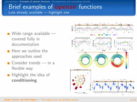
Brief examples of openair functionsLots already available — highlight one

Wide range available —covered fully indocumentation

Here we outline theapproaches used

Consider trends — in aflexible way

Highlight the idea ofconditioning



Mann-Kendall analysis of trendsConsider trends in NOX concentrations at London Bloomsbury

Mann-Kendall analysis often usedfor environmental time series

Consider monthly trends withoption to de-seasonalise the data

Use bootstrap simulationtechniques to estimate uncertaintiesand block bootstrap to deal withautocorrelation

year

NO

X

20

40

60

80

1998 2000 2002 2004 2006 2008

−1.43 [−2.03, −0.85] units/year ***

Example

Read some data in and plot the trendmydata = import(“d:/data/bloomsbury.csv”)

MannKendall(mydata, pollutant = “nox”, deseason = TRUE)



Mann-Kendall analysis of trendsTrends by wind sector

year

NO

X50

100

150

200

2501.08 [0.21, 1.8] units/year **

NW

1998 2000 2002 2004 2006 2008

−1.52 [−2.48, −0.67] units/year ***

N−1.26 [−2.04, −0.4] units/year **

NE

−0.31 [−0.87, 0.27] units/year

W

50

100

150

200

250−2.41 [−3.44, −1.33] units/year ***

E

50

100

150

200

250

1998 2000 2002 2004 2006 2008

−2.45 [−2.86, −1.9] units/year ***

SW−3.31 [−3.9, −2.7] units/year ***

S

1998 2000 2002 2004 2006 2008

−4.57 [−5.49, −3.6] units/year ***

SE

ExampleMannKendall(mydata, pollutant = “nox”, deseason = TRUE, type = “wd”)



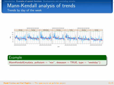
Mann-Kendall analysis of trendsTrends by day of the week

year

NO

X

20

40

60

80

100

120

1998 2000 2002 2004 2006 2008

−1.38 [−2.09, −0.64] units/year ***

Monday

1998 2000 2002 2004 2006 2008

−1.48 [−2.21, −0.66] units/year ***

Tuesday

1998 2000 2002 2004 2006 2008

−1.06 [−2.01, −0.11] units/year **

Wednesday

1998 2000 2002 2004 2006 2008

−1.78 [−2.51, −1.14] units/year ***

Thursday

1998 2000 2002 2004 2006 2008

−2 [−2.88, −1.26] units/year ***

Friday

1998 2000 2002 2004 2006 2008

−1.32 [−1.98, −0.62] units/year ***

Saturday

1998 2000 2002 2004 2006 2008

−1 [−1.57, −0.43] units/year ***

Sunday

ExampleMannKendall(mydata, pollutant = “nox”, deseason = TRUE, type = “weekday”)



Mann-Kendall analysis of trendsTrends by hour of the day

year

NO

X

20

40

60

80

100

120 −1.06 [−1.53, −0.58] units/year ***

00

199820002002200420062008

−0.88 [−1.41, −0.3] units/year ***

01−0.85 [−1.39, −0.36] units/year ***

02

199820002002200420062008

−0.7 [−1.22, −0.21] units/year ***

03−0.95 [−1.43, −0.39] units/year ***

04

199820002002200420062008

−0.95 [−1.52, −0.32] units/year **

05−1.44 [−2.16, −0.75] units/year ***

06

199820002002200420062008

−2 [−2.86, −1.21] units/year ***

07

−2.13 [−3.02, −1.35] units/year ***

08−1.79 [−2.6, −0.96] units/year ***

09−1.51 [−2.45, −0.67] units/year ***

10−1.34 [−2.14, −0.53] units/year ***

11−1.26 [−1.83, −0.68] units/year ***

12−1.13 [−1.7, −0.51] units/year ***

13−1.24 [−1.79, −0.65] units/year ***

14

20

40

60

80

100

120−1.28 [−1.89, −0.67] units/year ***

15

20

40

60

80

100

120

199820002002200420062008

−1.68 [−2.31, −1.06] units/year ***

16−2.05 [−2.77, −1.32] units/year ***

17

199820002002200420062008

−2.01 [−2.75, −1.29] units/year ***

18−1.96 [−2.72, −1.27] units/year ***

19

199820002002200420062008

−1.81 [−2.48, −1.14] units/year ***

20−1.96 [−2.63, −1.3] units/year ***

21

199820002002200420062008

−1.87 [−2.49, −1.16] units/year ***

22−1.35 [−1.9, −0.75] units/year ***

23

ExampleMannKendall(mydata, pollutant = “nox”, deseason = TRUE, type = “hour”)



Mann-Kendall analysis of trendsTrends by season

year

NO

X

40

50

60

70

80

1998 2000 2002 2004 2006 2008

−1.5 [−3.34, −0.27] units/year *

autumn

1998 2000 2002 2004 2006 2008

−1.82 [−4.95, 0.97] units/year

spring

1998 2000 2002 2004 2006 2008

−1.12 [−3.04, 0.95] units/year

summer

1998 2000 2002 2004 2006 2008

−0.35 [−1.28, 0.5] units/year

winter

ExampleMannKendall(mydata, pollutant = “nox”, deseason = TRUE, type = “season”)



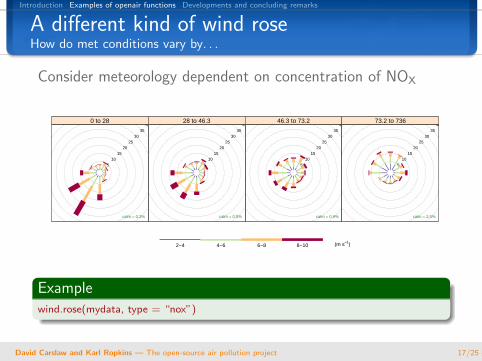
A different kind of wind roseHow do met conditions vary by. . .

Consider meteorology dependent on concentration of NOX

510

1520

2530

3540

4550

5560

calm = 0.2%

0 to 28

510

1520

2530

3540

4550

5560

calm = 0.5%

28 to 46.3

510

1520

2530

3540

4550

5560

calm = 0.9%

46.3 to 73.2

510

1520

2530

3540

45

calm = 2.0%

73.2 to 736

2−4 4−6 6−8 8−10 (m s−−1)

Examplewind.rose(mydata, type = “nox”)



How do concentrations vary by time?Looking at interventions

hour

NO

2 (p

pb)

20

25

30

35

40

0 6 12 18 23

Monday

0 6 12 18 23

Tuesday

0 6 12 18 23

Wednesday

0 6 12 18 23

Thursday

0 6 12 18 23

Friday

0 6 12 18 23

Saturday

0 6 12 18 23

Sunday

before 1 Jan. 2003 after 1 Jan. 2003

hour

NO

2 (p

pb)

25

30

35

0 6 12 18 23

month

NO

2 (p

pb)

24

26

28

30

32

34

J F M A M J J A S O N D

●

●

●

● ●

●

●● ●

●

●

●

●

● ●

●

●

●

●

●

●

●

● ●

weekday

NO

2 (p

pb)

26

28

30

32

34

Mon Tue Wed Thu Fri Sat Sun

●

●

●

●●

●

●

●

●

●

● ●

●

●

Examplemydata = split.by.date(mydata, date = “1/1/2003”, labels = c(“before 1 Jan. 2003”,

“after 1 Jan. 2003”))

time.variation(mydata, pollutant = “no2”, type = “site”, ylab = “no2 (ppb)”)



Tools for model evaluationCMAQ model output

Evaluating models isimportant

Emphasis is on quantitative‘metrics’ e.g. fractional bias

Scope for betterunderstanding of modelperformance

hour

O3

(ppb

)

20

25

30

35

0 6 12 18 23

Monday

0 6 12 18 23

Tuesday

0 6 12 18 23

Wednesday

0 6 12 18 23

Thursday

0 6 12 18 23

Friday

0 6 12 18 23

Saturday

0 6 12 18 23

Sunday

O3observed O3modelled

hour

O3

(ppb

)

20

25

30

0 6 12 18 23

month

O3

(ppb

)

20

25

30

35

J F M A M J J A S O N D

●

●●

●

●

●

●

●

●

● ●

●

●

●

●

●

●

●

●●

●

●

● ●

weekday

O3

(ppb

)

24

26

28

30

32

Mon Tue Wed Thu Fri Sat Sun

●●

●

●

●●

●

●

●

●●

●

●

●

Example

time.variation(cmaq, pollutant = “o3”, type = “site”)a

aThanks to Sean Beevers, King’s College London for CMAQ output.



Outline

1 Introduction





Higher time resolution measurementsWhat are the benefits?

Loss of useful informationwith hourly mean data

Measurements of NOX closeto Heathrow Airport

Hourly means show broadvariation in sourceemissions10-second measurementsreveal individual aircraftplumesMany new insightsa

aCarslaw et al. (2008). Near-field commercial aircraftcontribution to nitrogen oxides by engine, aircraft type andairline by individual plume sampling. ES&T. 42(6): 1871-1876.

hourly mean NOX concentrations

date

NOX

(ppb

)

0

50

100

150

19−Oct 20−Oct 21−Oct 22−Oct

10−second spot NOX concentrations

timeN

OX

(ppb

)

0

100

200

300

400

500

23:20:00 23:30:00 23:40:00 23:50:00



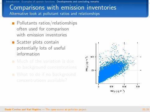
Comparisons with emission inventoriesAlternative look at pollutant ratios and relationships

Pollutants ratios/relationshipsoften used for comparisonwith emission inventories

Scatter plots containpotentially lots of usefulinformation

Much of the variation is dueto background concentrations

What to do if no backgroundconcentrations available?



Comparisons with emission inventoriesAlternative look at pollutant ratios and relationships

Pollutants ratios/relationshipsoften used for comparisonwith emission inventories

Scatter plots containpotentially lots of usefulinformation

Much of the variation is dueto background concentrations

What to do if no backgroundconcentrations available?

0 200 400 600 800 1000 1200 1400

0

50

100

150

NOX (µµg m−−3)

PM10(µµgm−−3)

12358111621283748617694114139166

background PMconcentration

10



Search for linear patterns in the dataEstimation of pollutant ratios in the absence of background data

Split data into 3-hournon-overlapping blocksa

Fit regression line to each3-hour block and calculateslopeFilter for slopes with highR2

⇒ Linear patterns in data

Mode of slope is a goodestimate of mean PM10/NOX

ratio

aBentley, S.T. (2003). Graphical techniques for constrainingestimates of aerosol emissions from motor vehicles using airmonitoring network data. Atmos. Env., 1491–1500.

NOX (µµg m−−3)

PM

10 (

µµg m

−−3)

20

40

60

200 400 600 800



Search for linear patterns in the dataEstimation of pollutant ratios in the absence of background data

Split data into 3-hournon-overlapping blocksa

Fit regression line to each3-hour block and calculateslopeFilter for slopes with highR2

⇒ Linear patterns in data

Mode of slope is a goodestimate of mean PM10/NOX

ratio

aBentley, S.T. (2003). Graphical techniques for constrainingestimates of aerosol emissions from motor vehicles using airmonitoring network data. Atmos. Env., 1491–1500.

PM10

NOX

(mass basis)

Per

cent

of T

otal

0

1

2

3

4

5

0.05 0.10 0.15

mode = 0.07 (kg/kg)



Developments

1 Reviewing scientific literature and will adopt promisingapproaches e.g.

Source identification and characterisationBetter quantitative analysisFurther development of tools for model evaluation

2 The openair package

Graphical-user interface (GUI)?1

Remote repository with full version control and easierinstallationWork towards access via AURN archive and LAQNReproducible analyses using Sweave, R and LATEX

1A researcher from another university has started this. . .



Thank you for you attention. . .

Questions?

David [email protected]


the open-source air pollution project - openairairtrack.lancs.ac.uk/carslaw.pdf · the open-source...

Documents